2012, Lund

Lund University

Lund Institute of Technology Division of Production Management

Department of Industrial Management and Logistics

Benefits of Multi-Echelon Inventory Control

A case study at Tetra Pak

Author: Oskar Räntfors

Supervisors: Johan Marklund, LTH

Jonas Schmidt

I

ABSTRACT

This thesis studies a two-echelon distribution inventory system with a central depot which

supplies N non-identical retailers with a single product. Stochastic customer demand

occurs solely at the retailers. The purpose of the master thesis project is to evaluate the

potential benefit of two methods in which the control of the inventory points in the

inventory system is coordinated. The two models of coordinated control are benchmarked

against a widely used single stage (uncoordinated) method.

Comparisons of the solutions produced by the methods are done using a discrete event

simulation model based on real inventory data. The effectiveness of the models are

evaluated in terms of the resulting total system cost, the average inventory levels, and

different types of service levels.

The simulation results clearly indicate that the evaluated methods for coordinated control

of inventories can offer considerable savings in reduced inventory levels and even, in many

cases, at the same time increasing the fill rate. The reductions in total cost range 11-37%

and an increase in fill rate accompanied by a reduction of the holding costs is observed in

most cases. Especially the holding costs at the Central Warehouse can be reduced; when

using a method for coordinated control the fill rate for orders from the retailers is 16-71%

which corresponds to a reduction of the CW holding costs of 50-94%.

II

FOREWORD

This master thesis is the concluding chapter of my journey to become a Master of Science

in Industrial Engineering. The project has been done in collaboration with an ERP systems

supplier who wishes to remain anonymous and Tetra Pak Technical Services who wanted

to know more about coordinated control in multi-echelon inventory systems. For me, this

has been a very rewarding journey, the analytical skills I have absorbed during my four

years at Lund Institute of Technology has been tested to the maximum.

A would like to take this opportunity to thank my supervisor Johan Marklund at LTH, his

help and support has been essential for this master thesis. I would also like to thank all of

you that was always helpful and provided important input at the anonymous ERP systems

supplier, you know who you are. A special thank goes to Jörgen Siversson at Tetra Pak for

supplying the crucial inventory data. I am also grateful to Christian Howard for supplying

me with his Extend model.

III

CONTENTS

1. INTRODUCTION ..................................................................................................................... 1

1.1. Background to inventory control in a multi-echelon system ........................................ 1

1.2. The studied inventory system and methods for coordinated control .......................... 3

1.3. Problem definition ......................................................................................................... 5

1.4. Method .......................................................................................................................... 6

1.5. Outline of the report ..................................................................................................... 7

2. THEORETICAL FRAMEWORK .................................................................................................. 8

2.1. Inventory control theory ............................................................................................... 8

2.1.1. Concepts ................................................................................................................ 8

2.1.2. Normally distributed demand ............................................................................. 10

2.1.3. Poisson process ................................................................................................... 10

2.1.4. Compound poisson demand ............................................................................... 11

2.1.5. Gamma distribution............................................................................................. 12

2.1.6. Optimal reorder points for an continuous review (R, Q) policy .......................... 14

2.2. Multi-echelon inventory systems ................................................................................ 17

2.2.1. Uncoordinated control of multi-stage inventory systems .................................. 18

2.3. Coordinated multi-echelon inventory optimization methods .................................... 19

2.3.1. The considered multi-echelon models - preliminaries ........................................ 19

2.3.2. Model 1: Heuristic coordination of a decentralized inventory systems using

induced backorder costs ..................................................................................................... 21

2.3.3. Model 2: Approximate optimization of a two-echelon distribution inventory

system 26

3. METHOD OF EVALUATION ................................................................................................... 30

3.1. Simulation model ........................................................................................................ 30

3.2. Selecting test cases ...................................................................................................... 31

3.3. Supply in-data for the simulation ................................................................................ 32

3.3.1. Virtual retailer ..................................................................................................... 34

3.3.2. Calculate reorder levels ....................................................................................... 34

3.4. Output data analysis .................................................................................................... 35

4. RESULTS AND DISCUSSION .................................................................................................. 36

4.1. Base cases .................................................................................................................... 37

IV

4.2. Sensitivity analysis ....................................................................................................... 40

4.2.1. Eliminate direct upstream demand ..................................................................... 40

4.2.2. Demand mean, transporting times and batch quantities ................................... 42

4.2.3. Target service levels ............................................................................................ 47

4.2.4. Homogenous / Heterogenic demand structure .................................................. 48

5. CONCLUSIONS AND FUTURE RESEARCH ............................................................................. 51

6. Appendix .............................................................................................................................. 53

6.1. Appendix A .................................................................................................................. 53

6.2. Appendix B................................................................................................................... 54

6.3. Appendix C ................................................................................................................... 56

6.4. Appendix E ................................................................................................................... 57

References ................................................................................................................................... 61

1

1. INTRODUCTION

Supply Chain Management, the control of the material flow from suppliers of raw material

to final customers, is today widely recognized as a crucial activity in most enterprises. The

interest in coordinated control of multi-stage inventory systems in most supply chains is

growing rapidly. A reason for this is that during the last two decades the research in this

area has progressed substantially; many early models, which were rather restrictive in their

assumptions, have been replaced by quite general ones. The new information technology

has also greatly increased the possibilities for effective use of these models. Still, in practice

today, there are very few examples of applications of the new research even though multi-

echelon systems are common. This can be explained by the fact that the methods are quite

difficult to understand and there are few illustrations of the benefits that coordinated

control may bring in real cases. This master thesis aims to provide such an illustration by

evaluating newly researched methods for coordinated inventory control using a simulation

model based on real inventory data.

This study was initiated by an ERP system supplier who wishes to remain anonymous, and

the inventory data required for the simulation models was acquired from Tetra Pak

Technical Services. Tetra Pak Technical Services provide technical expertise, services and

support in the areas of food processing and food packaging. They offer installation and

start-up services at a new plant; customized solutions within maintenance, verification, and

parts together with improvement services to enhance the performance; they also offer

training services for operators, maintenance personnel and managers. The inventory

system in question has its central warehouse in Lund and is handling spare parts for food

processing and packaging machinery.

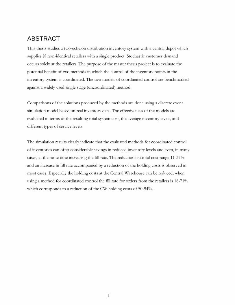
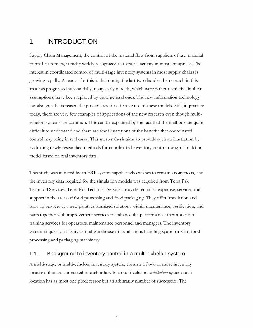
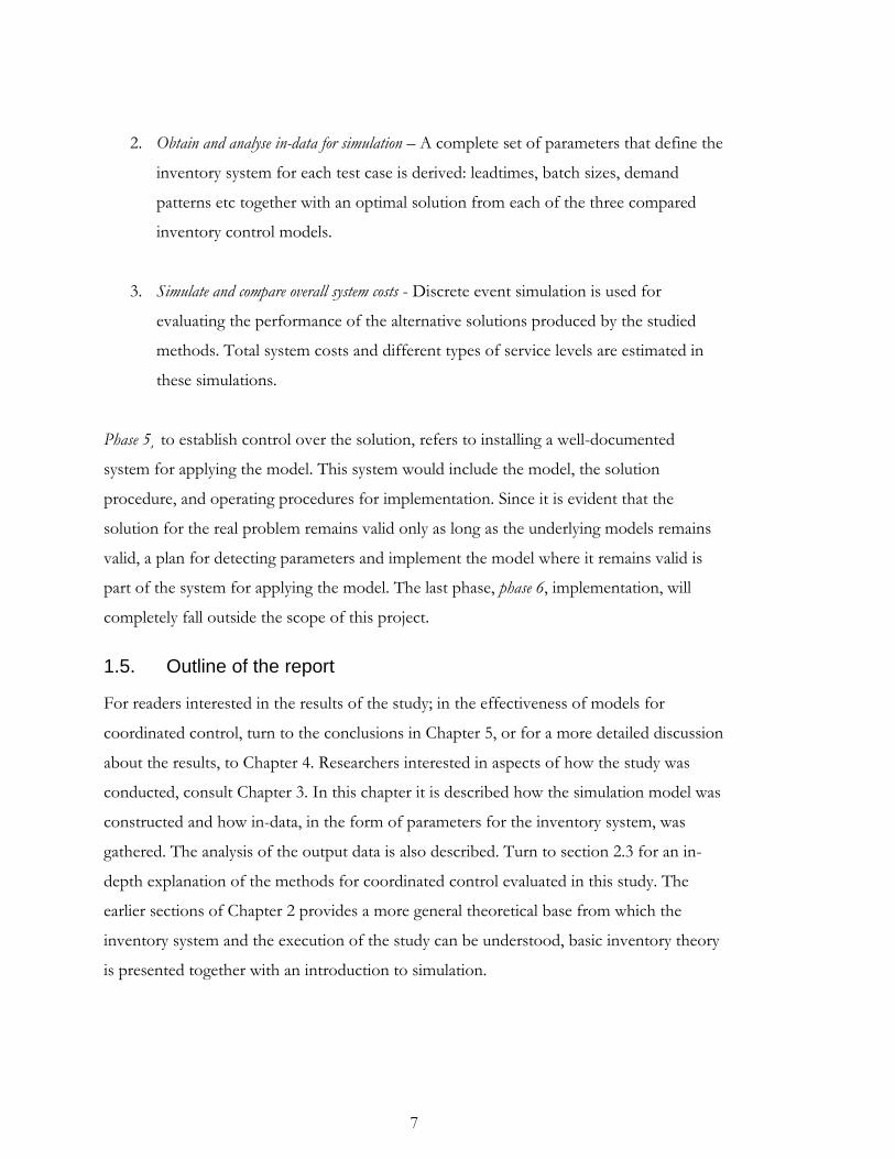
1.1. Background to inventory control in a multi-echelon system

A multi-stage, or multi-echelon, inventory system, consists of two or more inventory

locations that are connected to each other. In a multi-echelon distribution system each

location has as most one predecessor but an arbitrarily number of successors. The

2

complexities of managing inventory for such system increases significantly compared to

the single-echelon case.

Figure 1.1 A single-echelon inventory system and a two-echelon distribution system.

Before indulging in the challenges of multi-echelon systems let us review the single-echelon

problem, as seen in Figure 1.1. To control this inventory system one must make decisions

about which items to stock; how much stock to keep on hand; how often to inspect the

inventory; when to buy; how much to buy; controlling pilferage and damage; and managing

shortages and back orders. This is what inventory control is about and the ultimate

objective is to reduce the cost of the distribution, taking into account both costs associated

with keeping products in stock, holding costs, and costs associated with not being able to

satisfy customer demand directly, shortage costs. To narrow the scope of this master thesis

the focus lies on one of these questions: When to buy? A common way to answer this

question is to use the (R, Q) policy. This policy implies that a batch of Q units is ordered

when the inventory position (stock on hand + outstanding orders – backorders) drops to, or

below, the reorder point of R units. Therefore, to set a value for R is to answer the

question of when to replenish. By assuming continually inspected inventories (the time

between inspections is zero) the question on when to order is answered. The approaches

for finding an optimum ordering policy is well known for the single echelon case (Axsäter,

2006), they depend on a series of factors:

- Demand forecast.

- Leadtime to the external supplier

- Service level goal

3

But how should you set the control variables in the multi-echelon case? Today, enterprises

typically apply the single-echelon approach to each stock point in the system without

explicitly considering how decisions at one stock point affects the others; we refer to this

as an uncoordinated control of a multi-echelon system. Two questions arise:

- How much stock should be kept at the warehouse and at the different retailers?

- How do shortages at the warehouse affect the retailer leadtime?

The two questions are related, they have to do with the dynamics of the system; if you

reduce the service level of the warehouse, the risk of shortages will increase and therefore

the risk that an order from a retailer is delayed. As a result, the average retailer leadtime will

increase. Since those dynamics are impossible to take into account when the coupled

inventories are treated as independent there is no scientific way to determine the

warehouse service level. The uncoordinated approach will thus result in suboptimal

solutions often with excess inventory.

We now turn to the more advanced methods for control of multi-echelon inventory

systems, which we refer to as methods for coordinated control. There exists no completely

general method that works in all types of systems. The method depends on the

characteristics of the inventory system in question, such as: The physical properties of the

system, i.e., how the installations are coupled to each other, the size of the system, for

example, larger systems with high demand generally require approximate methods, as exact

methods tend to be computationally very demanding. Another aspect that governs the

choice of model is whether the system is controlled centralized or decentralized. For an

introduction on multi-echelon theories see Axsäter’s Inventory Control (2006).

1.2. The studied inventory system and methods for coordinated control

The considered inventory system is a two-level distribution system, which consists of one

central warehouse to which an arbitrarily number of retailers, N, are connected, see Figure

1.1. Customer demand takes place at the retailers, which replenish their stock from the

warehouse. The warehouse in turn places its orders with an outside supplier. The

replenishment leadtime from the outside supplier is fixed. Stockouts at both echelons are

4

fully backordered. This means that in case of a stock-out the customer waits until the

demand is fulfilled. Deliveries are made on a first-come first-serve basis – i.e. demand is

satisfied in the order it arrives. Transportation times are constant but retailer leadtimes are

stochastic due to possible shortages at the warehouse. All facilities use continuous review

(R,Q)-policies. This means that when the local inventory position (stock on hand +

outstanding orders – backorders) at the facility i decline to or below Ri, a replenishment

order of Qi units is placed. The objective is to optimize the reorder points Ri, i=0, 1, 2 …

N (0 corresponds to the central warehouse), the batch quantity and other inventory

parameters are given and fixed. Also, indications are that to assume predetermined and

fixed order quantities will only have a marginal effect on the expected cost, provided that

the reorder cost is adjusted accordingly and that the given order quantities are not too far

off, see for example Zheng (1992) and Axsäter (1996).

The two multi-echelon methods chosen to be evaluated in this study are both developed at

the division of production management at Lund Institute of Technology. The first method,

which will be denoted as Method 1 in the report, is the result from a series of three

publications. The first article (Andersson et al. 1998) introduces an induced backorder cost

at the warehouse, which will reflect the impact of the warehouse reorder level on the

retailer leadtime, and ultimately the end-customer service level. A somewhat

computationally demanding iterative procedure is used to find an optimal value for the

induced backorder cost. The introduction of the induced backorder cost enables a

decomposition of the multi-echelon system into a number of single echelon problems. The

model is based on a simple approximation, in which the stochastic leadtimes perceived by

the retailers are replaced by their correct averages. The method also assumes identical order

quantities at the retailers and normally distributed end customer demand. The second

article (Andersson & Marklund 2000) lifts the restriction of identical retailers. The third

(Berling & Marklund 2006) uses the iterative procedure developed in the first article to

build an intuitive understanding as to how the optimal induced backorder cost depends on

the system parameters, and uses this knowledge to create simple closed-form estimates of

the induced backorder, thus eliminating the computationally demanding iterative process in

the earlier publications.

5

The second method is based on Axsäter (2003), it is denoted as Method 2 in the report. It

uses normal approximations both for the retailer demand and the demand at the

warehouse, i.e., orders from the retailers. The normal approximations make it possible to

optimize even quite large systems effectively. The method also assumes that the mean and

variance for the delay at the warehouse, due to shortages, is the same for all retailers. The

general idea of the method is to (1) fit a normal distribution to the warehouse demand

mean and variation. (2) Determine mean and variance for the retailer leadtime for each

considered reorder level at the warehouse. (3) Determine each retailers optimum reorder

point for each of the considered warehouse reorder points. This is done through a simple

search procedure. (4) The optimum warehouse reorder level is determined by minimizing

the total system cost, which is now only dependent on the warehouse reorder point

(through step 3).

The uncoordinated approach that is evaluated in this project is an optimization method

found in a widely used commercial application developed by the ERP company that

initiated this study. This method is based on the standard techniques to optimize reorder

points in single-echelon system for example described in Axsäter (2006).

1.3. Problem definition

The purpose of this master thesis project is to investigate the performance of two models

for coordinated control in a multi-echelon inventory system, and thereby illustrate the

potential value of coordinated inventory control over the currently used uncoordinated

method.

Comparisons of the solutions produced by the methods are done using a discrete event

simulation model based on real inventory data. The effectiveness of the models are

evaluated in terms of the resulting total system cost, the average inventory levels, and

different types of service levels, in comparison with an uncoordinated approach.

6

1.4. Method

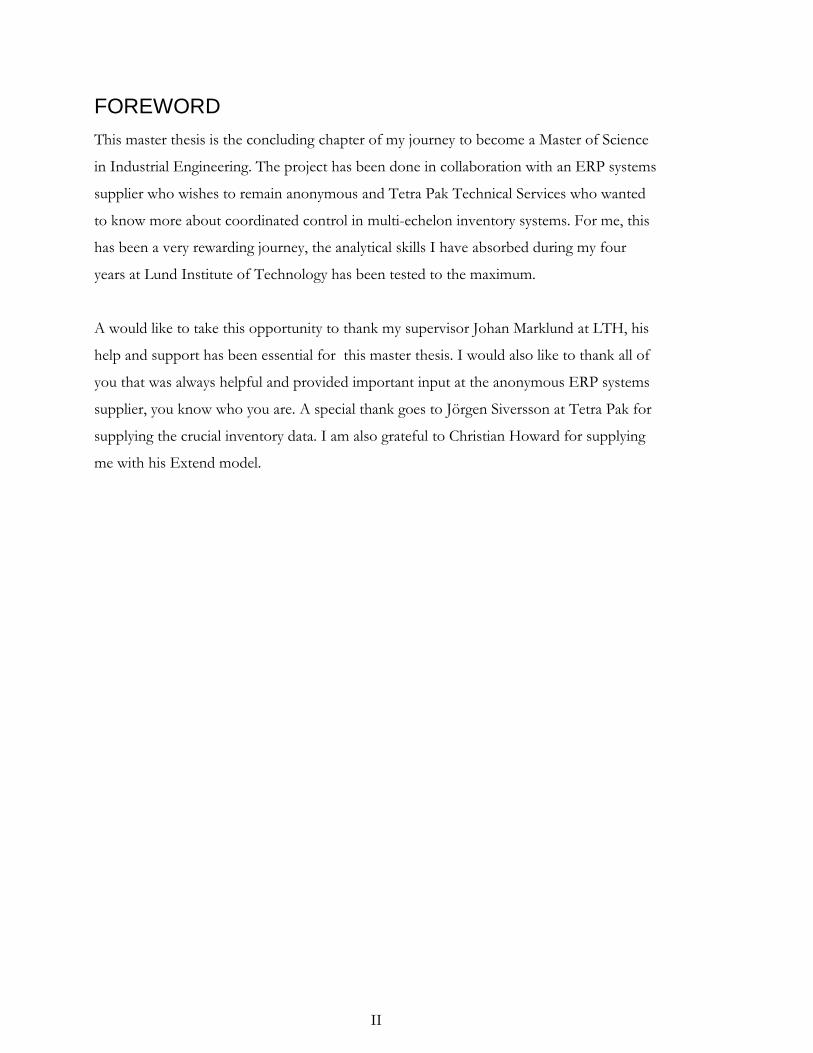
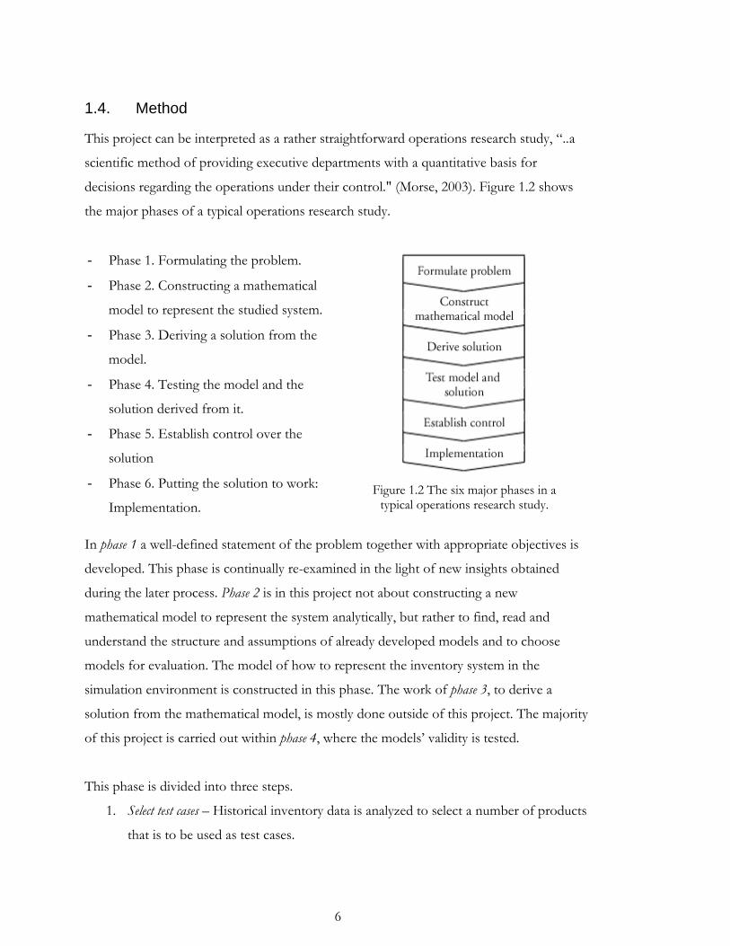
This project can be interpreted as a rather straightforward operations research study, “..a

scientific method of providing executive departments with a quantitative basis for

decisions regarding the operations under their control." (Morse, 2003). Figure 1.2 shows

the major phases of a typical operations research study.

- Phase 1. Formulating the problem.

- Phase 2. Constructing a mathematical

model to represent the studied system.

- Phase 3. Deriving a solution from the

model.

- Phase 4. Testing the model and the

solution derived from it.

- Phase 5. Establish control over the

solution

- Phase 6. Putting the solution to work:

Implementation.

Figure 1.2 The six major phases in a typical operations research study.

In phase 1 a well-defined statement of the problem together with appropriate objectives is

developed. This phase is continually re-examined in the light of new insights obtained

during the later process. Phase 2 is in this project not about constructing a new

mathematical model to represent the system analytically, but rather to find, read and

understand the structure and assumptions of already developed models and to choose

models for evaluation. The model of how to represent the inventory system in the

simulation environment is constructed in this phase. The work of phase 3, to derive a

solution from the mathematical model, is mostly done outside of this project. The majority

of this project is carried out within phase 4, where the models’ validity is tested.

This phase is divided into three steps.

1. Select test cases – Historical inventory data is analyzed to select a number of products

that is to be used as test cases.

7

2. Obtain and analyse in-data for simulation – A complete set of parameters that define the

inventory system for each test case is derived: leadtimes, batch sizes, demand

patterns etc together with an optimal solution from each of the three compared

inventory control models.

3. Simulate and compare overall system costs - Discrete event simulation is used for

evaluating the performance of the alternative solutions produced by the studied

methods. Total system costs and different types of service levels are estimated in

these simulations.

Phase 5¸ to establish control over the solution, refers to installing a well-documented

system for applying the model. This system would include the model, the solution

procedure, and operating procedures for implementation. Since it is evident that the

solution for the real problem remains valid only as long as the underlying models remains

valid, a plan for detecting parameters and implement the model where it remains valid is

part of the system for applying the model. The last phase, phase 6, implementation, will

completely fall outside the scope of this project.

1.5. Outline of the report

For readers interested in the results of the study; in the effectiveness of models for

coordinated control, turn to the conclusions in Chapter 5, or for a more detailed discussion

about the results, to Chapter 4. Researchers interested in aspects of how the study was

conducted, consult Chapter 3. In this chapter it is described how the simulation model was

constructed and how in-data, in the form of parameters for the inventory system, was

gathered. The analysis of the output data is also described. Turn to section 2.3 for an in-

depth explanation of the methods for coordinated control evaluated in this study. The

earlier sections of Chapter 2 provides a more general theoretical base from which the

inventory system and the execution of the study can be understood, basic inventory theory

is presented together with an introduction to simulation.

8

2. THEORETICAL FRAMEWORK

This chapter presents the theoretical base from which the inventory system and the

evaluation of the multi-echelon optimization models can be understood. Section 2.1 starts

with a number of definitions of concepts in inventory theory, then the theory used later in

the report is provided in section 2.1.2-2.1.4; the Poisson process, the compound Poisson

process and the gamma distribution. Expressions for optimizing reorder levels in a single-

echelon inventory system are given in section 2.1.5. Section 2.2 and onwards focuses on

inventory theory for the multi-echelon case. It begins with an overview of multi-echelon

inventory systems, and then discusses traditional methods for control of this system and

their strengths and weaknesses. Section 2.3 presents the theory for the two multi-echelon

models we consider.

2.1. Inventory control theory

This section focuses on the theoretical framework for controlling single-echelon inventory

systems.

2.1.1. Concepts

This is a short introduction to the basic concepts used in inventory control theory, for a

more in-depth treatment see for example the book Inventory Control (Axsäter 2006). To

begin with, a few central concepts in inventory control are defined.

Stock on hand – The number of physical items found in the defined inventory facility.

Backorder – A record of a customer order that could not be fulfilled immediately and is

waiting to be delivered.

Outstanding orders – Items ordered from the supplier that has not yet been delivered to the

inventory location in question.

Leadtime – The time from the ordering decision until the ordered amount is available for

demand on the shelves.

9

Holding cost – The cost for holding stock. The opportunity cost for capital tied up in

inventory usually makes the dominant part of this cost. Other parts can be material

handling, storage, damage and obsolescence, insurance and taxes. The holding cost per unit

and time unit is often determined as a percentage of the unit value.

Shortage costs – Costs occur when demanded items cannot be delivered due to shortages. In

some situations the customer agrees to wait, in other situations the customer chooses some

other supplier.

Service level goal – In most cases the costs associated with shortages are difficult to estimate;

therefore it is very common to replace them by a suitable service level constraint or target

service level. In practice there are many ways to define a service level and measure service,

the three most common are: (1) Probability of no stockout in an order cycle. (2) “fill rate”

– fraction of demand that can be satisfied immediately from stock on hand. (3) “ready rate”

– fraction of time with positive stock on hand.

Inventory position – Ordering decisions are based on the inventory position,

inventory position = stock on hand + outstanding orders – backorders.

Inventory level – Holding and shortage costs is based on the inventory level,

inventory level = stock on hand – backorders.

Continuous review / Periodic review – An inventory control system can be designed so that the

inventory position is monitored continuously and decisions made as changes occur, this is

called continuous review. An alternative, which is often motivated by the cost of

continuous supervision, is to monitor the inventory position only at certain given points in

time. In general, the intervals between these points are constant, this is called periodic

review. Continuous review will reduce the needed safety stock since this stock only have to

guard against demand variations during the leadtime. With periodic review the uncertainty

10

time is extended by the review period. Consider a review when no order is triggered. The

next possible delivery is the leadtime plus one review period ahead.

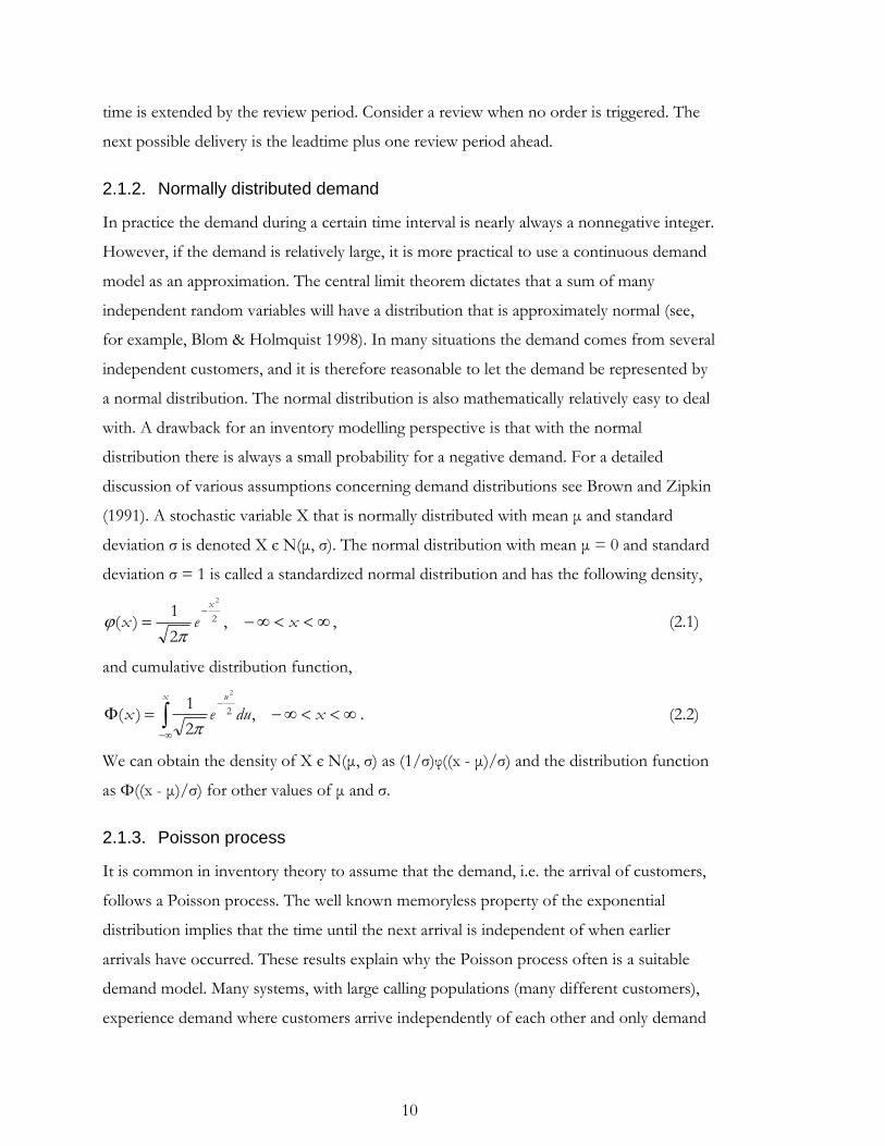
2.1.2. Normally distributed demand

In practice the demand during a certain time interval is nearly always a nonnegative integer.

However, if the demand is relatively large, it is more practical to use a continuous demand

model as an approximation. The central limit theorem dictates that a sum of many

independent random variables will have a distribution that is approximately normal (see,

for example, Blom & Holmquist 1998). In many situations the demand comes from several

independent customers, and it is therefore reasonable to let the demand be represented by

a normal distribution. The normal distribution is also mathematically relatively easy to deal

with. A drawback for an inventory modelling perspective is that with the normal

distribution there is always a small probability for a negative demand. For a detailed

discussion of various assumptions concerning demand distributions see Brown and Zipkin

(1991). A stochastic variable X that is normally distributed with mean μ and standard

deviation σ is denoted X є N(μ, σ). The normal distribution with mean μ = 0 and standard

deviation σ = 1 is called a standardized normal distribution and has the following density,

xexx

,2

1)( 2

2

, (2.1)

and cumulative distribution function,

xduex

x u

,2

1)( 2

2

. (2.2)

We can obtain the density of X є N(μ, σ) as (1/σ)φ((x - μ)/σ) and the distribution function

as Φ((x - μ)/σ) for other values of μ and σ.

2.1.3. Poisson process

It is common in inventory theory to assume that the demand, i.e. the arrival of customers,

follows a Poisson process. The well known memoryless property of the exponential

distribution implies that the time until the next arrival is independent of when earlier

arrivals have occurred. These results explain why the Poisson process often is a suitable

demand model. Many systems, with large calling populations (many different customers),

experience demand where customers arrive independently of each other and only demand

11

one unit at a time. The popularity of the process can also be explained by the fact that the

memoryless property simplifies analytical calculations.

Definition

Let k be the number of arrivals in the time interval (0, t). A stochastic process X(t), t ≥ 0, is

a Poisson process if the following three conditions are met:

1. The process has independent increments, i.e. the number of arrivals in disjoint

time intervals are independent.

2. P(there are exactly one arrival in the interval (t, t+h)) = λh + o(h).

3. P(there are more than one arrivals in the interval (t, t+h)) = o(h)

The Poisson process is said to have the intensity λ, which is also known as the arrival rate.

Two interesting results can be derived from these conditions. First, for a given t, the

number of arrivals in the time interval (0, t) is Poisson distributed with mean and variance

λt, i.e. the probability distribution of X(t) is given by

...).2,1,0(!

)()( xe

x

txP t

x

X

(2.3)

Second, the time between two arrivals is exponentially distributed with mean 1/λ, i.e. the

density function for the time between consecutive arrivals is given by

).0()( tetP t (2.4)

Proofs of these results can be found in e.g. Blom (1998).

2.1.4. Compound poisson demand

To make the simulations realistic a generalization of the poisson demand process is used

when describing the demand in the simulation environment. The customers arrive

according to a poisson process but the size of the customers’ orders is stochastic. The

quantity is assumed independent of other customer demands and of the distribution of the

customer arrivals. The discrete distribution of the demand size is denoted the

compounding distribution. Let

fj probability of demand size j (j=1, 2, …)

12

fjk probability that k customers give the total demand j

D(t) stochastic demand in the time interval t

We assume that there are no demands of size zero. This is no lack of generality, in both

cases such demand processes can be replaced by an equivalent process without those

characteristics. To determine D(t) we first note that f00 = 1, and fj

1 = fj. Given fj1 we can

obtain the j-fold convolution of fj, fjk, recursively as

...,4,3,2k,fff1j

1ki

ij

1k

i

k

j

(2.5)

Using (2.3) we then have

.fe!k

)t()j)t(D(P k

j

t

0k

k

(2.6)

If K is the stochastic number of customers during a time unit, J the stochastic demand size

of a single customer, and Z the stochastic demand during the time unit considered. Since K

is generated through a poisson process E(K) = Var(K) = λ, and K and J are independent

the mean and variance for the demand per time unit, μ, is given through

1

)()()(j

jjfJEKEZE . (2.7)

1

222 .)(j

jfjJE (2.8)

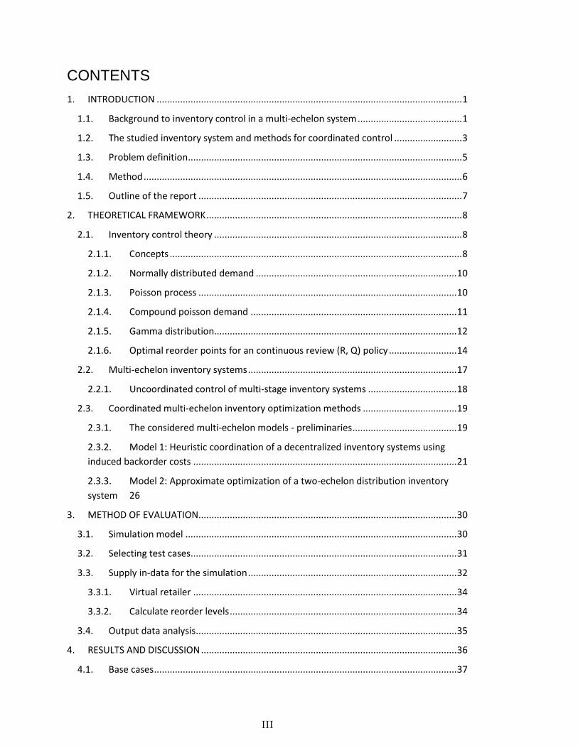
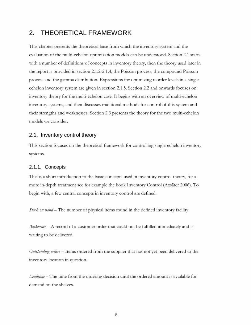
2.1.5. Gamma distribution

In the simulation environment a discrete distribution that is based on the gamma

distribution is used as the compounding distribution in the compound poisson demand

process. The gamma distribution, that is continuous, is converted to a discrete distribution

by rounding the stochastic variable up to nearest integer (see section 3.2).

The gamma distribution is defined by the probability density function (pdf) fX(x) and the

cumulative distribution function (cdf) FX(x)

13

00

0)(

1

)(

/1

xif

xifexpa

xf

axp

p

X (2.9)

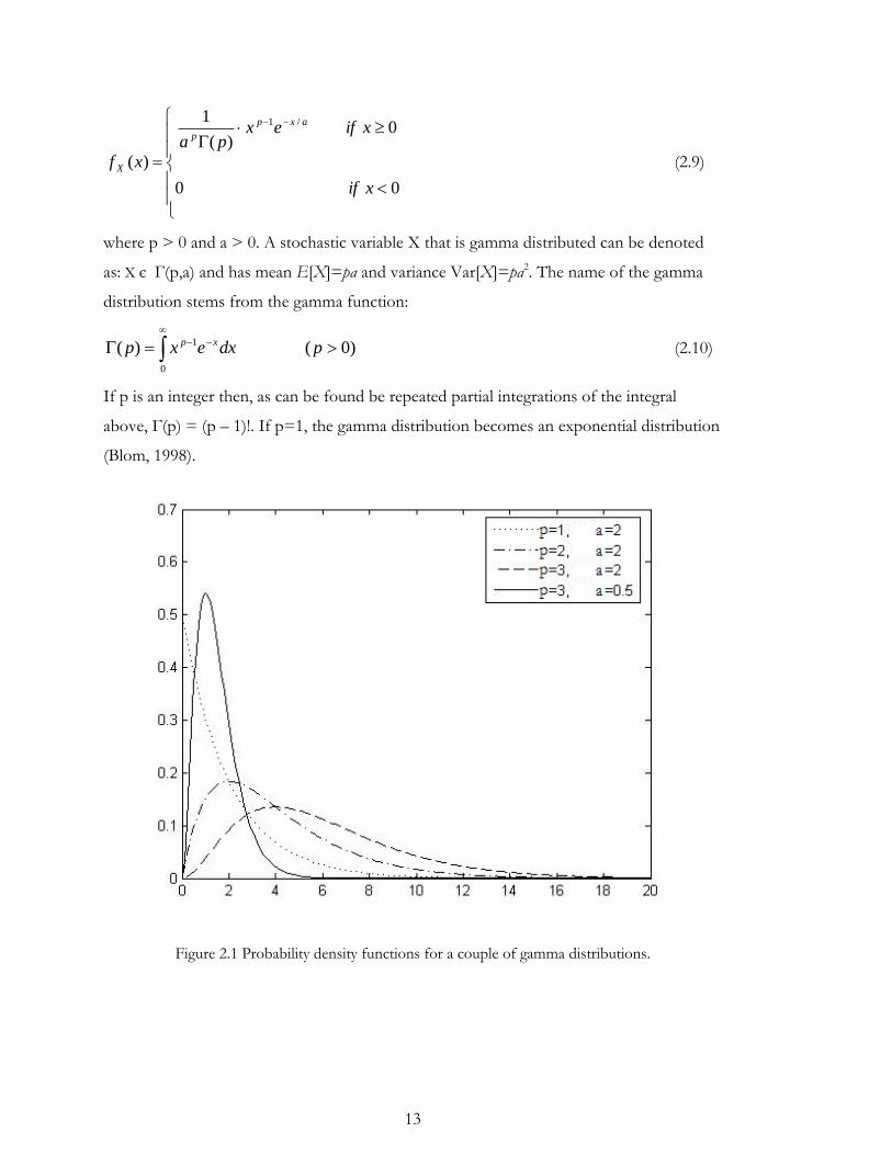
where p > 0 and a > 0. A stochastic variable X that is gamma distributed can be denoted

as: X є Γ(p,a) and has mean E[X]=pa and variance Var[X]=pa2. The name of the gamma

distribution stems from the gamma function:

)0()(0

1

pdxexp xp (2.10)

If p is an integer then, as can be found be repeated partial integrations of the integral

above, Γ(p) = (p – 1)!. If p=1, the gamma distribution becomes an exponential distribution

(Blom, 1998).

Figure 2.1 Probability density functions for a couple of gamma distributions.

14

2.1.6. Optimal reorder points for an continuous review (R, Q) policy

An ordering policy is the set of rules that control when and how much to order at an

inventory location. The continuous review (R, Q) policy implies that the inventory position

is inspected continually and that a batch of Q units is ordered at the instant that the

inventory position reaches R units. The parameter R is referred to as the reorder point and

Q as the ordering quantity or the batch quantity.

When implementing the (R, Q) policy, the objective is to determine the two parameters; the

reorder point and the ordering quantity. How to determine ordering quantity lies outside

the scope for this master thesis, this parameter will be treated as given. To determine an

optimal reorder point we need to balance the need to minimize holding costs with the need

to provide adequate service. This is either done through a prescribed service level goal, or

by defining holding costs and shortage costs. We will assume that the demand is normally

distributed. The process of finding an optimal reorder point is only discussed briefly here,

for more details see Axsäter (2006) chapter 5, which this section follows quite closely.

Used notation:

IL inventory level

f(x) density function for the inventory level

F(x) distribution function for he inventory level

φ(x) The normal density function

Φ(x) The normal distribution function

S2 Service level goal, fill rate

S3 Service level goal, ready rate

μ Mean for the leadtime demand

σ Standard deviation for the leadtime demand

h Holding cost

b Backorder cost

Using a service level constraint

In section 2.1.1, three different service level definitions are given. Here we will only

consider the last two, fill rate (S2) and ready rate (S3). These are the constraints that is used

15

by Tetra Pak. Under the assumption of normally distributed demand S2 = S3, and the

service level is the probability of positive stock. Using the so called loss function,

x

xxxdvvxvxG ))(1()()()( , (2.11)

the distribution function for the inventory level can be given by

QR

R

xu

QxF

1

1)( du

uxuG

Q

QR

R

1

xQRG

xRG

Q. (2.12)

The service level can now be obtained from

QRG

RG

QFSS 10132 . (2.13)

For a given service level we can search for the smallest R rendering the required service

level.

Using holding costs and shortage costs

We optimize the reorder point by minimizing the sum of expected holding and backorder

costs. It is convenient to use the notation

(x)+ = max(x, 0) and (x)−= max(-x, 0). (2.14)

Note that x+ - x- = x. The expected cost per unit of time is given by

)()( ILbEILhEC )()()( ILEbhILhE

0

)()()2/( dxxFbhQRh

dudxxu

GQ

bhQRh

QR

R

01

)()2/(

QR

R

duu

GQ

bhQRh

)()2/( . (2.15)

16

In the first line of (2.15) we use that the average inventory position is R + Q/2 in the

continuous case. Furthermore,

0 000 0

)()()()()( dxxFdxduufdxdxufduuufILE

x

u

(2.16)

We now need to define the function H(x),

)()(112

1)( 2 xxxxdvvGxH

x

.

Note that H´(x) = - G(x). We can now express the cost in (2.15) as

QRH

RH

QbhQRhC

2

)()2/( . (2.17)

To find the optimal reorder point we now need to minimize (2.17) with respect to R. From

(2.17) and (2.13) and the definition of H(x) we have

)1)(()( 2

Sbhh

QRG

QRG

Qbhh

dR

dC

32 )()( SbhbSbhb . (2.18)

Since C is a convex function of R, the optimal R is obtained for dC/dR = 0.

Relationship between cost parameters and service level

In the optimal solution for (2.18) we have

bh

bSS

32 . (2.19)

Since it is often the relation between holding costs and backorder cost that is of interest,

the holding cost can be set to one. Then, if a service level, S2, is given, (2.19) can be used to

find a backorder cost. The backorder cost can in turn be used to find an optimal reorder

level which will render the desired service level. In the case of compound Poisson demand

this relation is only valid for the ready rate and it becomes

1** 33

RSbh

bRS . (2.20)

(2.20) is also valid for the fill rate in case of pure Poisson demand, when each customer

only orders one item.

17

2.2. Multi-echelon inventory systems

A multi-echelon inventory system consists of several inventory locations that are connected

to each other. They appear in practice both when distributing products over large

geographical areas and in production, where stocks of raw material, components, and

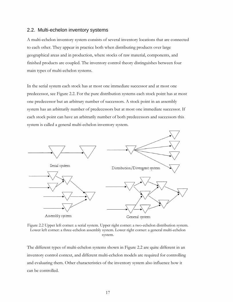
finished products are coupled. The inventory control theory distinguishes between four

main types of multi-echelon systems.

In the serial system each stock has at most one immediate successor and at most one

predecessor, see Figure 2.2. For the pure distribution systems each stock point has at most

one predecessor but an arbitrary number of successors. A stock point in an assembly

system has an arbitrarily number of predecessors but at most one immediate successor. If

each stock point can have an arbitrarily number of both predecessors and successors this

system is called a general multi-echelon inventory system.

Figure 2.2 Upper left corner: a serial system. Upper right corner: a two-echelon distribution system. Lower left corner: a three-echelon assembly system. Lower right corner: a general multi-echelon

system.

The different types of multi-echelon systems shown in Figure 2.2 are quite different in an

inventory control context, and different multi-echelon models are required for controlling

and evaluating them. Other characteristics of the inventory system also influence how it

can be controlled.

18

- High / Low demand. Systems with high demand generally require approximate

methods, as exact methods tend to be computationally very demanding.

- Repairable / Consumable items. Repairable items needs to be transported upstream

in the system.

- Centralized / Decentralized organization. Is each stock point included in single

organization so that they can be regulated centrally or are the administrated by a

multiple number of independent organizations.

- Lateral transshipments. Items can be transported between parallel stock points in

order to avoid shortages.

I will now focus on the two-echelon distribution system, for consumable items. For

simplicity, no lateral transhipments will be regarded. For a more detailed introduction of

different types of multi-echelon systems and models see, for example, van Houtum et al

(1996).

2.2.1. Uncoordinated control of multi-stage inventory systems

As previously mentioned we refer to an uncoordinated approach to control multi-stage

inventory systems when single-echelon models are used to control stocks that are in fact

connected and interdependent. Each stock point in the system is treated as independent

with a set leadtime and service level, optimal reorder points is then determined using a

forecast for the demand at this site.

The obvious strength of this method is its simplicity, multi-echelon method are in general

much more complex. The weakness is that it does not describe the real system in an

adequate way and obvious interdependencies in the system are not taken into account, and

as a result suboptimal solutions are produced.

In an uncoordinated approach two problems arise: (1) How we should determine the

warehouse demand, this demand is in fact fully determined by the retailer demand and to

do an extra forecast introduces an extra layer of error and a risk for bullwhip effect. (2)

Since we assume that the purpose of the system is to serve the end-customer, the question

is to deploy the safety stock in the system in the most efficient way to achieve this objective

19

in time. How should then the service level for the warehouse be set? The choice of service

level goal at the warehouse will affect the leadtime to the retailer. With a low central

inventory, orders from the retailers will often be delayed and, as a result, it may be

necessary to increase the retailers reorder points. In an uncoordinated approach the last

remark is not taken into account and the resulting solution will thus be suboptimal.

2.3. Coordinated multi-echelon inventory optimization methods

2.3.1. The considered multi-echelon models - preliminaries

The two considered methods deal with approximate optimization of the reorder points for

continuous review (R, Q) policies in a two-echelon distribution inventory system. The

batch quantities are assumed to be given. The stochastic customer demand occurs at the

retailers. It is stationary with known mean and standard deviation, and is independent

across retailers and over time. The retailers replenish their stock from the warehouse, and

the warehouse in turn places its order with an outside supplier with supposedly infinite

stock. Stockouts at both echelons are backordered and delivered on a first-come first-serve

basis. All transportation times are constant but the retailer leadtimes are stochastic because

of delays due to shortages at the warehouse. Also, to minimize the long run average system

costs with respect to reorder points, the investigated methods use a cost structure with

linear holding cost and shortage costs.

The following notation will be used for both methods.

N number of retailers

li constant transportation time for an order to arrive at retailer i from the warehouse

L0 constant leadtime for an order to arrive at the warehouse from the outside supplier

q largest common factor of Q0, Q1, Q2, …,QN, i.e., q is the largest positive

integer such that all batch quantities are integer multiples of q (q may correspond to a

package size or could be 1), this factor is referred to as a subbatch.

Qi batch size at retailer i, expressed in units

Q0 batch size at the warehouse, expressed in units

hi holding cost per unit and time unit at retailer i

h0 holding cost per unit and time unit at the warehouse

20

pi shortage cost per unit and time unit at retailer i;

Ri reorder point for retailer i

R0 warehouse reorder point expressed in units of q

Ci expected cost per time unit at retailer i

C0 expected warehouse cost per time unit

C expected total system cost per unit of time

μi(t) mean of the demand at retailer i during time period t

Vari(t) variance of the demand at retailer i during during time period t

μi expected demand per time unit at retailer i

μ0 expected demand per time unit at the warehouse Σi μ i

Vari variance of the demand per time unit at retailer i

Var0 variance of the demand per time unit at the warehouse

pi,k(L0) probability for k orders at retailer i during the warehouse leadtime

μiw(L0) average demand from retailer i at the warehouse during the warehouse

leadtime

Variw(L0) variance of the demand from retailer i at the warehouse during the

warehouse leadtime

μw(L0) average demand from the retailers at the warehouse during

the warehouse leadtime = Σi μw

i(L0)

Varw(L0) variance of the demand from the retailers at the warehouse during the

warehouse leadtime = Σi Varwi(L0)

D0(L0) stochastic demand at warehouse during leadtime, expressed in units

Also, standard notations for the standard deviation is used, σi = (Vari)1/2.

21

2.3.2. Model 1: Heuristic coordination of a decentralized inventory systems

using induced backorder costs

Introduction

The choice of a reorder level at the warehouse affects the retailers’ leadtimes, which in turn

influences the reorder level decisions at the retailers. To coordinate the control of the

inventories in the distribution system this method introduces an induced backorder cost, β,

which captures the impact that a reorder level decision at the warehouse has on the

retailers. When an appropriate induced backorder cost is determined it is possible to

optimize the reorder level at the warehouse. A relationship between the warehouse reorder

level and the retailers’ leadtimes can then be used to provide the lead-time estimate

necessary for optimizing the reorder points at the retailers.

The method builds on the results from three research papers: The first (Andersson et al.

1998) presents an iterative procedure to find an induced backorder that minimizes the

expected total system costs, β*. In this paper the stochastic retailer leadtimes are replaced

by their averages and all retailers are assumed to use a common batch quantity, Q0. For

general settings the iterative procedure is too computationally demanding in order to be

used commercially. The second paper (Andersson et al. 2000) develops the model to allow

for retailers to use individual ordering quantities. In the third paper (Berling & Marklund

2006) the iterative procedure in the first paper is used to build an understanding on how

the optimal induced backorder cost depends on the parameters of the inventory system.

This knowledge is then used to create closed form estimates which produce near-optimal

induced backorder costs that will be denoted as β*. An emphasis is placed on large systems

with high demand and/or many retailers for which existing methods are not

computationally feasible. The model assumes normally distributed demand and that, in

case of shortages, orders are shipped when they can be delivered in full.

The optimization of the reorder level is performed in 6 steps: (1) The warehouse demand

is determined (note that this is independent of the retailers’ reorder points). (2) The system

parameters are normalized. (3) The near-optimal induced backorder cost, β*, is determined

using the normalized system parameters. (4) A single-echelon method is used to determine

22

the optimal warehouse reorder point. (5) Given the optimized warehouse reorder level the

stochastic retailer leadtime is determined and then replaced with its average. (6) Finally, the

retailer reorder points can also be determined using ordinary single-echelon methods.

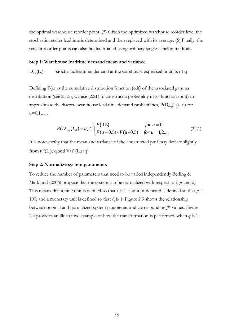
Step 1: Warehouse leadtime demand mean and variance

D0,q(L0) stochastic leadtime demand at the warehouse expressed in units of q

Defining F(x) as the cumulative distribution function (cdf) of the associated gamma

distribution (see 2.1.5), we use (2.21) to construct a probability mass function (pmf) to

approximate the discrete warehouse lead time demand probabilities, P(D0,q(L0)=u) for

u=0,1,….

,...2,1)5.0-(-)5.0(

0)5.0())(( 0,0

uforuFuF

uforFuLDP q

(2.21)

It is noteworthy that the mean and variance of the constructed pmf may deviate slightly

from w(L0)/q and Varw(L0)/q2.

Step 2: Normalize system parameters

To reduce the number of parameters that need to be varied independently Berling &

Marklund (2006) propose that the system can be normalized with respect to li, μi and hi.

This means that a time unit is defined so that li is 1, a unit of demand is defined so that μi is

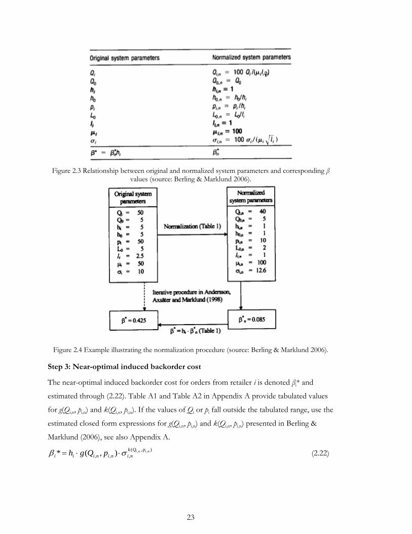
100, and a monetary unit is defined so that hi is 1. Figure 2.3 shows the relationship

between original and normalized system parameters and corresponding β* values. Figure

2.4 provides an illustrative example of how the transformation is performed, when q is 1.

23

Figure 2.3 Relationship between original and normalized system parameters and corresponding β values (source: Berling & Marklund 2006).

Figure 2.4 Example illustrating the normalization procedure (source: Berling & Marklund 2006).

Step 3: Near-optimal induced backorder cost

The near-optimal induced backorder cost for orders from retailer i is denoted βi* and

estimated through (2.22). Table A1 and Table A2 in Appendix A provide tabulated values

for g(Qi,n, pi,n) and k(Qi,n, pi,n). If the values of Qi or pi fall outside the tabulated range, use the

estimated closed form expressions for g(Qi,n, pi,n) and k(Qi,n, pi,n) presented in Berling &

Marklund (2006), see also Appendix A.

),(

,,,,,),(* nini pQk

nininiii pQgh (2.22)

24

A single induced warehouse backorder cost is estimated as a weighted average with respect

to the average demand rates.

**1 0

i

N

i

i

. (2.23)

Step 4: Optimal warehouse reorder point

The objective is to find a near optimal reorder point to the original system by minimizing

the expected holding and induced backorder costs at the central warehouse, C0(R0).

)R(C 00

y

u

q

QR

Ry

uLDPuyQ

qh

0

0,0

10

0 ))(()(*)( 00

0

q

LQRq

w )(

2

1* 00

0

(2.24)

It is easy to show that, as >0, )R(C 00 - )1-R(C 00 is increasing in R0, which implies that

)R(C 00 is convex. Thus an optimal R0

can therefore be found through a simple search

0≤)1-R(C-)R(C:RmaxR 00000*0 (2.25)

Step 5: Retailer leadtimes

Eq (2.26)-(2.28) provide an approach to approximate the average retailer leadtime

proposed in Andersson & Marklund (2000). Numerical observations have shown that a

large retailer in terms of μi and Qi tends to have longer mean leadtime, iL . In other words,

a retailer which orders often and in large quantities have, relatively speaking, more units

backordered and reserved at the warehouse than a retailer with low ordering frequency and

small order quantities. This step is more thoroughly described in Andersson and Marklund

(2000) section 5.2.

Define

iL expected lead-time for an order to arrive at retailer i

)( 0BE expected number of backorders at the warehouse in units of q

25

)( 0

rBE expected number of reserved subbatches at the warehouse

(ordered by a retailer at the central warehouse but not yet

shipped)

001 /)( qBE

mean delivery delay due to stockouts at the warehouse

002 /)( qBE r mean delivery delay due to reserved units waiting to be shipped

N

i

iii qQ1

)(

yu

0q,0

QR

1Ry00q,0)L(D

QR

1Ry00 )u)L(D(P)yu(

Q

1)y)L(D(E

Q

1BE

00

0

0q,0

00

0

(2.26)

i

iiii

i lqQNqQ

L

1

2

1

1

11

)()/()(

(2.27)

Where (x)+ = max(x, 0). The first two terms in (2.27) represent an estimate of the mean

delivery delay to retailer i due to stockouts at the warehouse and reserved units waiting to

be shipped respectively. The estimate is found by differentiating the average delivery delay

due to stockouts over all retailers based on the relative size of the retailer’s relative

deviation from the average retailer size, measured in terms of the product μi(Qi – Q), as a

basis for estimating the stockout delivery delay to that same retailer. The third term in

(2.27) represents an estimate of the mean delivery delay to retailer i due to the existence of

reserved units at the warehouse. The last term is the constant transportation time.

To get an explicit expression for )( 0

rBE Andersson & Marklund suggests another

approximation, inspired by an idea in Lee and Moinzadeh (1987). This approximation is

based on the observation that reserved units only occur when a fraction of a retailer’s order

quantity is backordered. In (2.28) Q can be interpreted as an average batch size. If we

divide the number of backordered units B0 by Q and the result is fractional, say 2.45, this

indicates, due to the complete delivery policy at the warehouse, that the total number of

delayed units is 3Q and subsequently that 0.55Q units are reserved at the warehouse.

26

Define

x the smallest integer >= x

N

i i

i

Q1

0

= Demand intensity at the warehouse in number of retailer orders

N

i

N

i

i

i

i

i QQ

Q1 1 00

)()( 0

0 o

r BEQQ

BEBE

(2.28)

Step 6: Optimal retailer reorder points

With an estimate in place the retailer reorder points can now be determined in analogy with

step 4 by minimizing (2.29) with respect to Ri.

i

iii

i

iii

iiiiii

QRH

RH

QbhQRhC

0

2

0 )()2/( (2.29)

2.3.3. Model 2: Approximate optimization of a two-echelon distribution

inventory system

Introduction

The method originates with Axsäter (2003) and is based on normal approximations for

both the retailer demand and the demand at the warehouse due to orders from the

retailers. The approximations make it computationally feasible to optimize by successively

searching for the set of reorder points that generates the least costs.

In short, the method can be described in six steps: (1) The warehouse demand mean and

variance is determined. (2) For each feasible warehouse reorder point, the mean and

variance for the retailer leadtime is determined. (3) Optimal retailer reorder levels for each

feasible warehouse reorder level are determined and total costs for each solution is

calculated. (4) The optimum warehouse reorder level is found by minimizing the total

27

costs. Both warehouse and retailer demand is assumed to follow normal distributions. An

excel macro that executes this inventory optimization algorithm can be found at:

http://www.iml.lth.se/Sven/Approximate%20Optimization.xls.

We define

μiLT mean of the stochastic leadtime faced by retailer i

VariLT variance of the stochastic leadtime faced by retailer i

Step 1: Warehouse leadtime demand mean and variance

First, the warehouse leadtime demand mean and variance, μw(L0) and Varw(L0) is

determined. To do this the probability for k orders at retailer i during the warehouse

leadtime, pi,k(L0), is approximated by

dxL

LQkx

L

LkQx

QLp

iQ

i

ii

i

ii

i

ki

00

0

0

0

0,)(

)()1(

)(

)(1)(

)(

)(2

)(

)()1(

)(

)()1()(

0

0

0

0

0

00

L

LkQG

L

LQkG

L

LQkG

Q

L

i

ii

i

ii

i

ii

i

i

, (2.30)

where G(x) is defined by (2.11) in section 2.1.6. Refer to Axsäter (2003) or Andersson et al

(1998) for details on how pi,k(L0) is derived. pi,k(L0) is determined for all k for which the

probability is not too low, k is under normal conditions a small number. It follows that

)()( 00 LL i

w

i and (2.31)

k

ki

w

ii

w

i LpLkQLVar 0,

2

00 )( , (2.32)

We now fit a normal distribution to the warehouse leadtime demand and determine its

mean and variance, μw(L0) and Varw(L0), by summing μiw(L0) and Vari

w(L0) over i.

Step 2: Mean and variance for retailer leadtimes

The mean and variance of the leadtime faced by the retailers are modelled as a function of

the warehouse reorder point R0, the delay is assumed to be equal for all retailers. Using

28

Little’s formula the mean leadtime for the retailers are obtained from the expected number

of backorders and the total demand,

N

i i

i

LT

i

IEl

1

0 )(

. (2.33)

The variance of the retailer leadtime can be expressed as

22 )()( EVar LT

i , (2.34)

where δ is the stochastic delay at the warehouse for retailer orders and μδ is its mean. The

mean and variance of the retailer leadtime are calculated for each feasible warehouse

reorder point R0. For a complete derivation of these equations, see Axsäter (2003).

Step 3: Optimize retailer reorder levels

A normal distribution is fitted to the retailer leadtime demand and μi(LT) and Vari(LT)

determined through,

i

LT

ii LT )( and (2.35)

LT

ii

LT

iii VarVarLTVar 2)()( . (2.36)

Optimal retailer reorder points are calculated for each feasible warehouse reorder point by

minimizing the retailer cost function,

)()(),( 0 iiiiii IEpIEhRRC . (2.37)

The formulas for the expected number of backorders and the expected stock level, E(Ii)-

and E(Ii)+ are omitted here (again, see Axsäter 2003). We denote the optimal reorder point

for a given R0 by Ri*(R0). Since Ci(R0, Ri) is a convex function in Ri given R0 (see Axsäter

2000) the minimum is found using a computationally fast search procedure over Ri.

Step 4: Optimal warehouse reorder level

In the last step the warehouse costs are calculated for each feasible warehouse reorder

point using

)()( 000 IEhRC o , (2.38)

where E(I0) is the expected inventory level. Now the optimal warehouse reorder point, R0,

and the corresponding optimal retailer points, Ri*(R0), are found by minimizing the total

cost function

29

))(,()()( 0

1

*

0000 RRRCRCRCN

i

ii

. (2.39)

Too make optimization fast we disregard that C(R0) is not necessarily convex and just look

for a local minimum.

30

3. METHOD OF EVALUATION

This chapter explains how the performances of the optimization methods were

investigated and compared. First a simulation model was constructed to represent the

inventory system in the testing phase, see Section 3.1. The inventory data was analysed and

three base cases selected, see Section 3.2. In-data to the simulation environment was

supplied using the inventory data and output (reorder points) from the three optimization

models, see Section 3.3. Lastly, the output data from the simulation was analysed to

compare the optimization methods, Section 3.4.

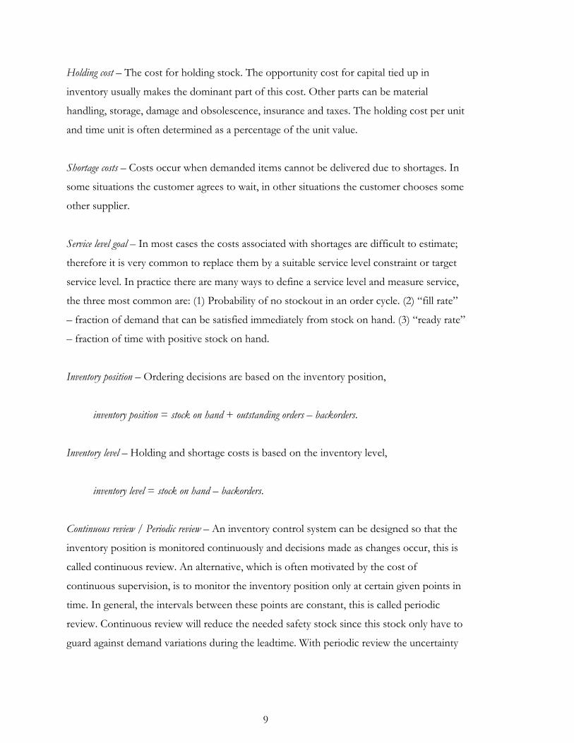
3.1. Simulation model

The simulation of the inventory system is performed using a discrete event simulation

model in the simulation software Extend. A reason for using a high-level programming

software like Extend is that considerable time can be saved in constructing the model.

Also, the foundation for the simulation model was already available through another

research project (Howard, C. 2007). The logic of a two-echelon inventory system, as

described in Section 1.2, was implemented in the simulation model. See Appendix D for

more information on the simulation environment.

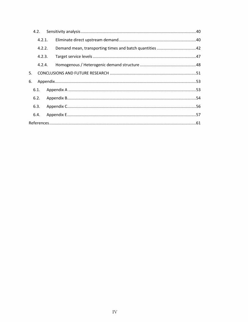
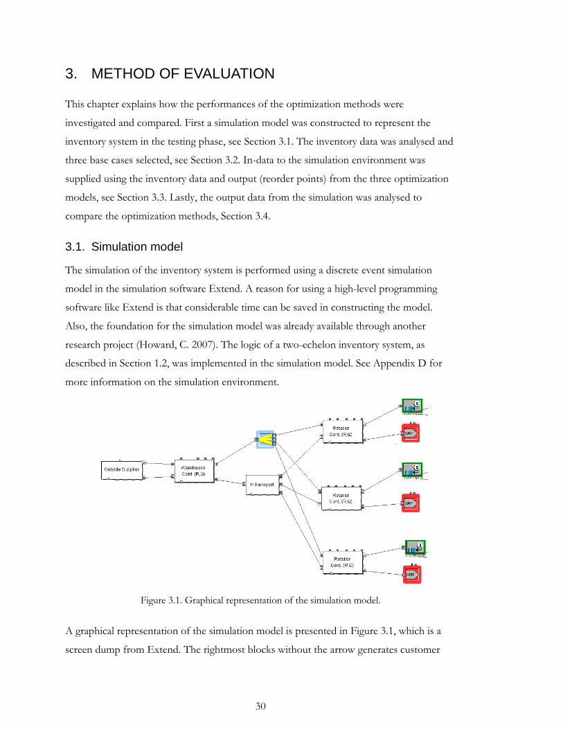
Figure 3.1. Graphical representation of the simulation model.

A graphical representation of the simulation model is presented in Figure 3.1, which is a

screen dump from Extend. The rightmost blocks without the arrow generates customer

31

events with an intensity and order sizes according to a compound Poisson process. As

described in Section 2.1.6 this process is often used to model demand data accurately, see

this section for a more thorough discussion. The customer event is sent to the connected

block labelled “Retailer Cont (R, Q)” which simulates a stock point governed by a

continuous review (R, Q) policy. The ordered items, represented by the customer events,

which can be delivered immediately exits to the right entering to the block marked with an

arrow, the ordered items that cannot be delivered are backordered. When the inventory

position of the stock point reaches its reorder point an order of size Q is generated and

sent to the block labelled “Warehouse Cont (R, Q)” which simulates a stock point in the

same way as the retailer block. The warehouse block treats incoming orders the same way

as the retailer block treats customer events. When an order (or part of an order) from a

retailer is fulfilled, a replenishment event is triggered and sent to the “In transport” block,

which delays the event for a set amount of time. After the event is delayed it is relayed to

the retailer block, where the stock is replenished by the amount of units set by the ordering

level of the retailer block. Order events triggered at the warehouse block is sent to the

block labelled “Outside supplier”, where the event is delayed for a set amount of time and

then sent back to the warehouse where the stock is replenished.

3.2. Selecting test cases

The inventory data supplied by Tetra Pak Technical Service AB in Lund was analysed to

find adequate test cases. The data contained information on 80 products, characterized as

spare parts, stocked in an inventory system that consisted of one central warehouse and 19

retailers. Few products were stocked at all 19 retailers. For each article and stock point the

data included the following information:

- Order quantity

- Transportation time (time to transport unit from supplier to stock point)

- Target service level (fill rate)

- Achieved service level (fill rate)

- Date, time and size for orders during a period of three years

Tetra Pak views the distribution system as a part of the value chain and therefore increases

the value of an item by 20% when it arrives at a retailer. The inventory data was analysed

32

statistically to provide an overview, tables and plots from this analysis is provided in

Appendix B. An interesting observation is that for most products a large portion of the

demand took place directly at the warehouse, a direct upstream demand. Three products

were selected to provide in-data for the simulation environment, for a specification see

Table 4.1 in Section 4.1, these items will be referred to as the base cases. The rationale

behind this selection was primarily the fact that it’s only relevant to evaluate the multi-

echelon models in conditions they are designed for. We know that, in their current form,

the methods are not designed for situations where the direct upstream demand is large or

the total system demand low; in those cases other methods should be used. Therefore, only

products where the total demand was more than five units/day and where the direct

upstream demand comprised less than 60% of the total demand was considered. Within

these limits the three products was selected to cover as much of the diversity in total

inventory system demand, number of retailers, total system demand and mean size of the

customer orders. All 80 products are plotted with respect to total demand and percentage

of direct upstream demand in Appendix B.

3.3. Supply in-data for the simulation

The following parameters are needed to provide in-data to the simulation model:

- Transportation times from the outside supplier to the warehouse and from the

warehouse to each retailer.

- Holding costs at all locations and shortage costs at all retailers.

- Ordering quantities for the warehouse and the retailers.

- Parameters for the compound Poisson process that generates the retailer demand.

- Reorder levels at the warehouse and each retailer.

The transportation times are readily available in the supplied inventory data and can be

used directly. The need for holding costs and shortage costs arise since Method 1 and 2 are

both, in their current form, so called backorder cost models. Since we are only interested in

the relative performance of the optimization models, the retailer holding cost is normalized

to 1 and, to accommodate for the fact that the value of the an item increases 20% when it

reach the retailer, the warehouse holding cost is set to 0.84.

33

The shortage cost was derived from the target service level, that is available in the supplied

inventory data, according to the process discussed in Section 2.1.6, Eq. (2.18) and (2.19).

As noted in this section this method only produces accurate results for the fill rate when

the demand is continuous or generated by a pure Poisson process. As the demand is

generated by a compound Poisson process in the simulation model, the translation process

will only be accurate when the service level is measured as a ready rate. This means that

Method 1 and Method 2 is in fact optimizing the reorder level with regard to the ready rate

(in the inventory data both the target and the achieved service level is measured with the

fill rate in mind). Since the same is true for the uncoordinated method, as it assumes

continuous demand, this does not constitute a problem when comparing the coordinated

optimization models of the backorder type with the uncoordinated method which uses a

service level constraint. However, there is an underlying problem of misalignment between

the target service level and the service level used in the optimization of the reorder points

for both the conventional single-echelon method and the investigated multi-echelon

models.

Even though a parameter for the order quantity was explicitly available in the inventory

data this value was not used when defining the test cases. The analysis of the inventory

data showed that the actual size of the replenishment orders from the retailers did not

follow the set order sizes. As the model assumes fixed order quantities the average of all

replenishment orders from a retailer was used when defining the order quantities actually

used in the test cases. The alternative, to fit the order quantities from the inventory data to

a distribution and then treat them stochastically in the simulation model was disregarded

for sake of simplicity. For the warehouse, the order quantity parameter available in the

inventory data is used without modification since there is no data for the order placed with

the outside supplier.

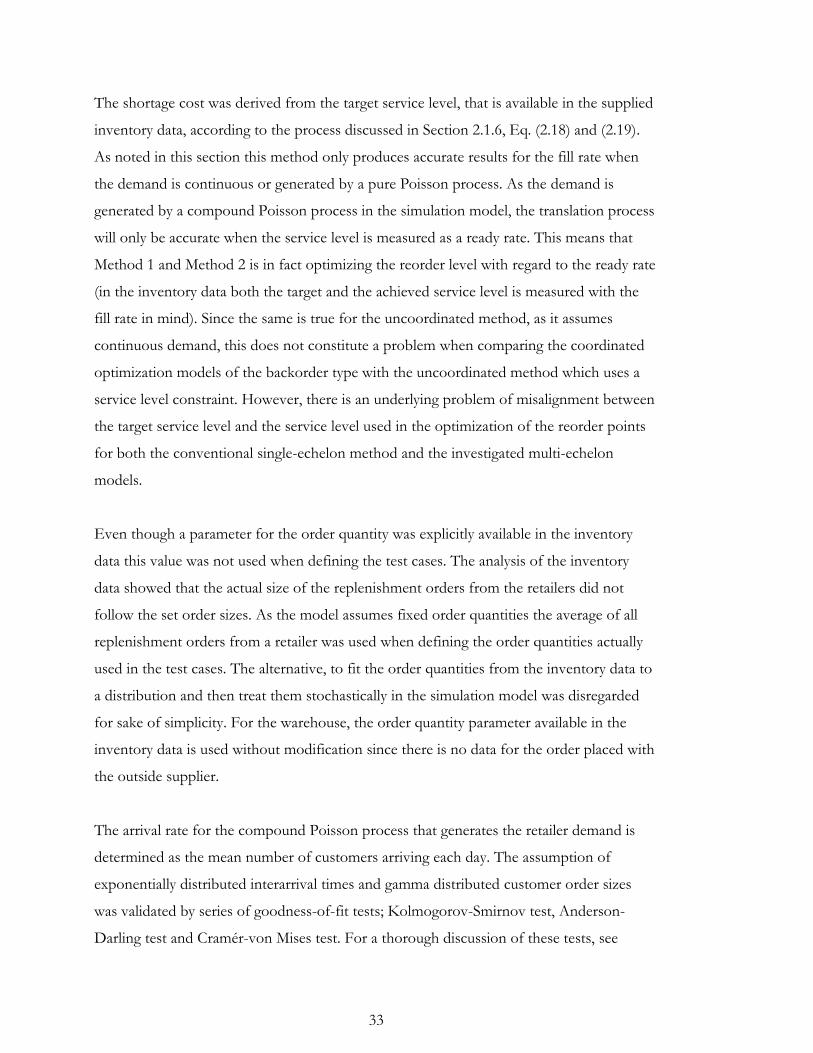
The arrival rate for the compound Poisson process that generates the retailer demand is

determined as the mean number of customers arriving each day. The assumption of

exponentially distributed interarrival times and gamma distributed customer order sizes

was validated by series of goodness-of-fit tests; Kolmogorov-Smirnov test, Anderson-

Darling test and Cramér-von Mises test. For a thorough discussion of these tests, see

34

D'Agostino and Stephens (1986). A discrete gamma distribution is fitted to the mean and

variation of the customer order sizes and used as the compounding distribution. The

gamma distribution was chosen because both its mean and variance can be varied through

its parameters, it is non-negative, and it proved a good fit with the data. Arrival intensity,

customer order sizes and demand data for the three test cases together with the resulting

demand parameters is presented in Appendix C.

3.3.1. Virtual retailer

As mention in section 3.2, a common feature in the analysed test data was that a large

portion of the customer demand takes place directly at the warehouse. This is sometimes

called direct upstream demand in the literature. The evaluated models for coordinated

control are not specifically constructed to handle this. The way around this dilemma is to

model the direct upstream demand as a separate retailer, a virtual retailer that is a separate

stock reserved for direct customer demand at the warehouse (see Axsäter 2007). The order

quantity for the virtual retailer is always 1 and the leadtime is set to 0. For the

uncoordinated approach the reorder level is always set to -1. This means that each

customer demand at the virtual retailer triggers a corresponding warehouse order of the

same size. There will never be any stock on hand at the virtual retailer in the uncoordinated

case. This is generally not true for a coordinated approach; in this case a reorder level is

determined in the same way as for the other retailers.

3.3.2. Calculate reorder levels

The last step when defining the test cases is to determine a set of reorder levels for each of

the evaluated optimization methods. Reorder levels are calculated for Method 1 and

Method 2 using software provided by Johan Marklund and Sven Axsäter respectively. For

the uncoordinated method, the SCP method, the order levels were calculated using

documentation received from the ERP company that initiated this project.

The simulated warehouse mean and variance is used as input when determining reorder

levels for the SCP Method. In real conditions, an extra forecast with accompanied forecast

error would have to be made at the warehouse. As this extra layer of error is eliminated by

providing the method with an exact value for the warehouse demand this provides a slight

35

advantage for the SCP method. It should be noted that for the virtual retailer, the

transportation time is naturally zero, but as the current form of method 1 cannot handle

such transporting times a number close to zero is used instead, unfortunately the resulting

reorder levels vary quite a bit depending on how close to zero this value is. The model was

reported to have been adjusted and allow for transporting times of zero in the end of this

project.

3.4. Output data analysis

Each test case was run for 400 000 time units (days) (200 000 time units for the sensitivity

tests), excluding a warm-up period of 5000 time units. Observations of output variables

were made every 40 000th time unit and then reset (every 20 000th time unit for the

sensitivity tests). The number of observations in a simulation run was determined by

minimizing the variance of the mean for the output variables; i e different time intervals

was tested and the obtained variance was compared. The length of the complete simulation

run was then set so that the variance of the mean was sufficiently low.

A set of output variables from the simulation was used to make comparisons between the

evaluated models:

- Mean holding cost for the system per time unit.

- Mean total system cost (holding cost and shortage cost) for the system per time unit.

- Ready rate, defined as the fraction of time with a positive stock on hand.

- Fill rate, defined as the fraction of demand that can be satisfied immediately from

stock on hand.

It could be argued that mean total system cost is the only output needed to make a

satisfactory comparison of the models, however most corporations use different kinds of

service levels, and not shortage costs, to measure inventory performance. The student’s t-

distribution was used to create confidence intervals for the output data and the t-test to

make significance tests.

36

4. RESULTS AND DISCUSSION

In this chapter the results from the simulations are presented and discussed. First, results

from the three base cases are presented and discussed in section 4.1. Direct upstream

demand is excluded in section 4.2.1. The results from a number of sensitivity tests is

presented and discussed in section 4.2.2 to 4.2.4. All discussed differences are significant at

a level of 95%.

Four performance measurements are used in the analysis: Ready rate (S3), fill rate (S2),

expected holding costs (HC) and total costs (TC). TC gives a balanced measurement of the

performance and is easily comparable, it is the preferred choice of measurement. In

practise S2 and HC are the most commonly used measurements. The ready rate is only

included in the sensitivity tests, it is included because, as discussed in Section 3.3, the

evaluated methods are in fact optimizing the reorder points with regard to meet the set

ready rate. S3 > S2 when the mean customer order is greater than one. The difference

between S2 and S3 grows larger as the mean customer order size increases. When referring

to averages for the retailer fill rate and ready rate in this section, it is the weighted average,

with respect to the retailed demand. The relationship between S2 and TC is complicated by

the fact that the shortage costs vary among the retailers; if S2 is increased at a retailer with a

high shortage cost the TC will decrease more than if the retailer had a low shortage cost.

HC and S3 have rather low variance in the simulations while the variances for TC and S2

are higher.

The following notations/abbreviations are used in this chapter.

CW central warehouse.

VR virtual retailer, a retailer that is created to model direct upstream

demand at the central warehouse (see section 3.3.1).

S2 average for the retailer fill rate, weighted with respect to demand.

S3 average for the retailer ready rate, weighted with respect to

demand.

HC average holding costs for the system

37

TC average total cost for the system (the sum of the expected holding

costs and the expected shortage costs)

M1 Method 1: Heuristic coordination (see section 2.3.2)

M2 Method 2: Approximate optimization (see section 2.3.3)

SCP A method for uncoordinated control used in a commercial system

for inventory control.

N Number of retailers.

L Transportation time

Q Ordering quantity or batch size

4.1. Base cases

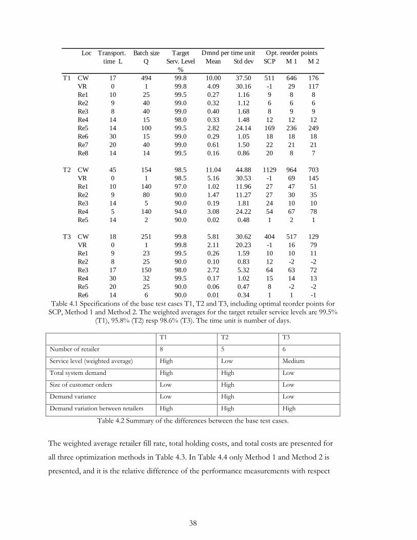
A detailed specification of the three base cases, T1-T3, is available in Table 4.1. There are a

few things worth noticing: For all three test cases the majority of the total customer

demand takes place in two of the retailers, of which the VR (see section 3.3.1) is one. The

portion of demand at the VR is between 40 and 60%. The transportation times (L) vary

considerably within each of the three test cases.

Test Case T1: Consists of eight retailers and, relative to the other test cases, a high

total mean demand. The customer order size is fairly low for all retailers, or,

equivalently, the variance for the retailer demand is relatively low. This test case has

a homogenous structure for the service level targets.

Test Case T2: Consists of five retailers and a relatively high total mean demand.

Since customer order sizes are generally very large, the variance for the retailer

demand is high. This test case also has a mix of high and low service level targets.

Test Case T3: Consists of six retailers and a relatively low total mean demand.

Customer order sizes and retailer demand variance are generally low. This test case

has a homogenous structure for the service level targets.

The service level targets for the retailers are generally high, for T1-T3 the weighted

averages are 99.5%, 95.8% resp 98.5%. These distinctions are summarized in Table 4.2.

More detailed specifications of the test cases are available in Appendix E.

38

Loc Transport. Batch size Target

time L Q Serv. Level Mean Std dev SCP M 1 M 2

%

T1 CW 17 494 99.8 10.00 37.50 511 646 176

VR 0 1 99.8 4.09 30.16 -1 29 117

Re1 10 25 99.5 0.27 1.16 9 8 8

Re2 9 40 99.0 0.32 1.12 6 6 6

Re3 8 40 99.0 0.40 1.68 8 9 9

Re4 14 15 98.0 0.33 1.48 12 12 12

Re5 14 100 99.5 2.82 24.14 169 236 249

Re6 30 15 99.0 0.29 1.05 18 18 18

Re7 20 40 99.0 0.61 1.50 22 21 21

Re8 14 14 99.5 0.16 0.86 20 8 7

T2 CW 45 154 98.5 11.04 44.88 1129 964 703

VR 0 1 98.5 5.16 30.53 -1 69 145

Re1 10 140 97.0 1.02 11.96 27 47 51

Re2 9 80 90.0 1.47 11.27 27 30 35

Re3 14 5 90.0 0.19 1.81 24 10 10

Re4 5 140 94.0 3.08 24.22 54 67 78

Re5 14 2 90.0 0.02 0.48 1 2 1

T3 CW 18 251 99.8 5.81 30.62 404 517 129

VR 0 1 99.8 2.11 20.23 -1 16 79

Re1 9 23 99.5 0.26 1.59 10 10 11

Re2 8 25 90.0 0.10 0.83 12 -2 -2

Re3 17 150 98.0 2.72 5.32 64 63 72

Re4 30 32 99.5 0.17 1.02 15 14 13

Re5 20 25 90.0 0.06 0.47 8 -2 -2

Re6 14 6 90.0 0.01 0.34 1 1 -1

Dmnd per time unit Opt. reorder points

Table 4.1 Specifications of the base test cases T1, T2 and T3, including optimal reorder points for

SCP, Method 1 and Method 2. The weighted averages for the target retailer service levels are 99.5% (T1), 95.8% (T2) resp 98.6% (T3). The time unit is number of days.

T1 T2 T3

Number of retailer 8 5 6

Service level (weighted average) High Low Medium

Total system demand High High Low

Size of customer orders Low High Low

Demand variance Low High Low

Demand variation between retailers High High High

Table 4.2 Summary of the differences between the base test cases.

The weighted average retailer fill rate, total holding costs, and total costs are presented for

all three optimization methods in Table 4.3. In Table 4.4 only Method 1 and Method 2 is

presented, and it is the relative difference of the performance measurements with respect

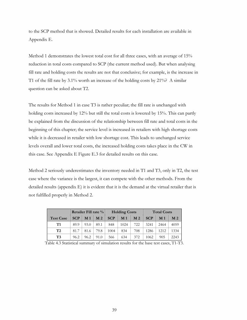
39

to the SCP method that is showed. Detailed results for each installation are available in

Appendix E.

Method 1 demonstrates the lowest total cost for all three cases, with an average of 15%

reduction in total costs compared to SCP (the current method used). But when analysing

fill rate and holding costs the results are not that conclusive; for example, is the increase in

T1 of the fill rate by 3.1% worth an increase of the holding costs by 21%? A similar

question can be asked about T2.

The results for Method 1 in case T3 is rather peculiar; the fill rate is unchanged with

holding costs increased by 12% but still the total costs is lowered by 15%. This can partly

be explained from the discussion of the relationship between fill rate and total costs in the

beginning of this chapter; the service level is increased in retailers with high shortage costs

while it is decreased in retailer with low shortage cost. This leads to unchanged service

levels overall and lower total costs, the increased holding costs takes place in the CW in

this case. See Appendix E Figure E.3 for detailed results on this case.

Method 2 seriously underestimates the inventory needed in T1 and T3, only in T2, the test

case where the variance is the largest, it can compete with the other methods. From the

detailed results (appendix E) it is evident that it is the demand at the virtual retailer that is

not fulfilled properly in Method 2.

Retailer Fill rate % Holding Costs Total Costs

Test Case SCP M 1 M 2 SCP M 1 M 2 SCP M 1 M 2

T1 89.9 93.0 89.1 848 1024 722 3241 2464 4059

T2 81.7 81.6 79.8 1004 834 708 1286 1212 1334

T3 96.2 96.2 91.0 566 634 372 1062 905 2243

Table 4.3 Statistical summary of simulation results for the base test cases, T1-T3.

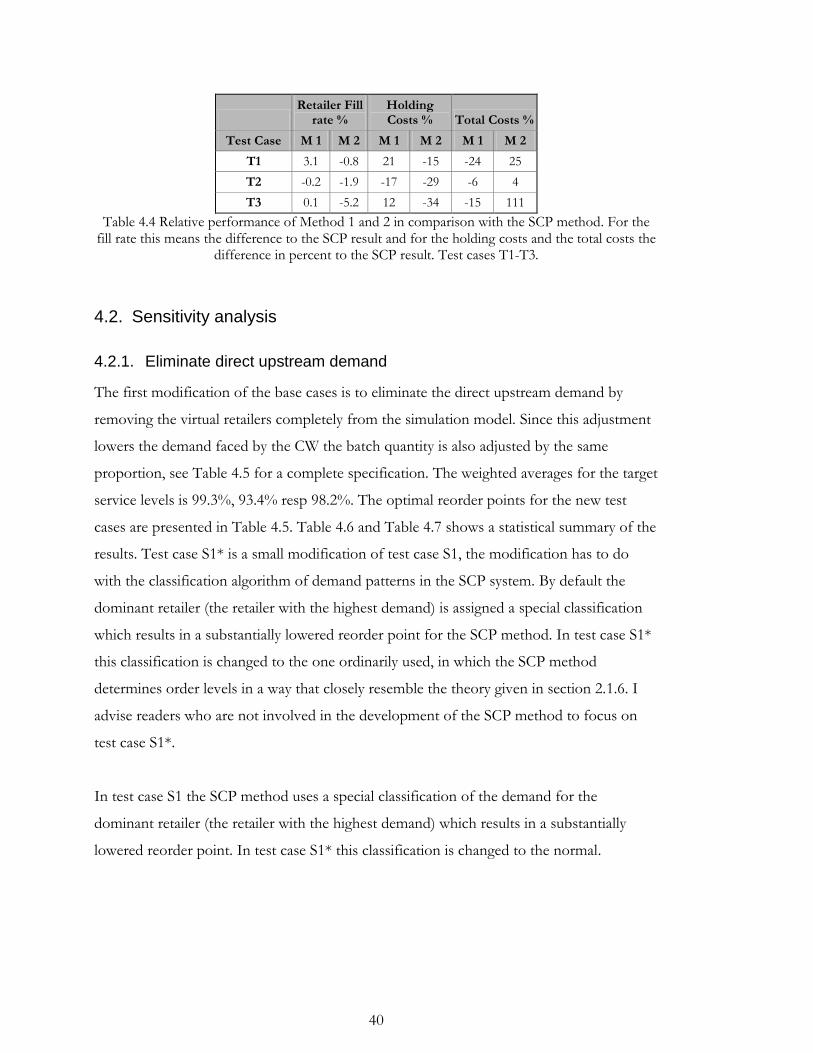
40

Retailer Fill

rate % Holding Costs % Total Costs %

Test Case M 1 M 2 M 1 M 2 M 1 M 2

T1 3.1 -0.8 21 -15 -24 25

T2 -0.2 -1.9 -17 -29 -6 4

T3 0.1 -5.2 12 -34 -15 111

Table 4.4 Relative performance of Method 1 and 2 in comparison with the SCP method. For the fill rate this means the difference to the SCP result and for the holding costs and the total costs the

difference in percent to the SCP result. Test cases T1-T3.

4.2. Sensitivity analysis

4.2.1. Eliminate direct upstream demand

The first modification of the base cases is to eliminate the direct upstream demand by

removing the virtual retailers completely from the simulation model. Since this adjustment

lowers the demand faced by the CW the batch quantity is also adjusted by the same

proportion, see Table 4.5 for a complete specification. The weighted averages for the target

service levels is 99.3%, 93.4% resp 98.2%. The optimal reorder points for the new test

cases are presented in Table 4.5. Table 4.6 and Table 4.7 shows a statistical summary of the

results. Test case S1* is a small modification of test case S1, the modification has to do

with the classification algorithm of demand patterns in the SCP system. By default the

dominant retailer (the retailer with the highest demand) is assigned a special classification

which results in a substantially lowered reorder point for the SCP method. In test case S1*

this classification is changed to the one ordinarily used, in which the SCP method

determines order levels in a way that closely resemble the theory given in section 2.1.6. I

advise readers who are not involved in the development of the SCP method to focus on

test case S1*.

In test case S1 the SCP method uses a special classification of the demand for the

dominant retailer (the retailer with the highest demand) which results in a substantially

lowered reorder point. In test case S1* this classification is changed to the normal.

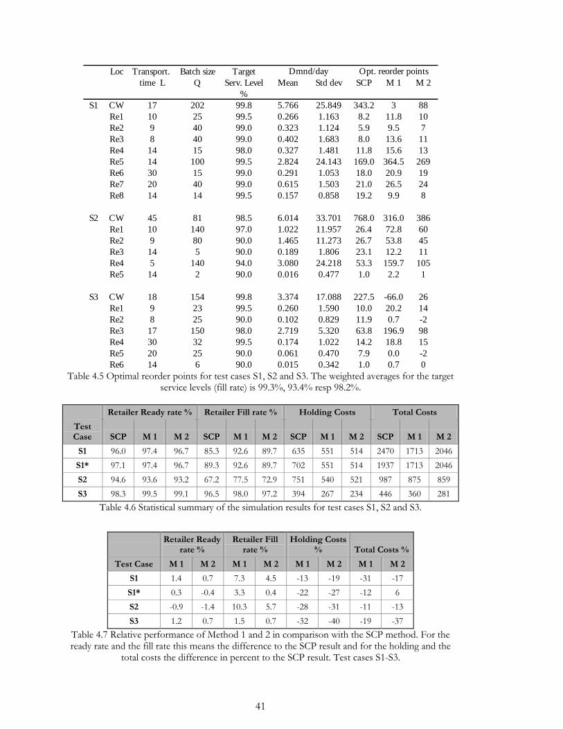
41

Loc Transport. Batch size Target

time L Q Serv. Level Mean Std dev SCP M 1 M 2

%

S1 CW 17 202 99.8 5.766 25.849 343.2 3 88

Re1 10 25 99.5 0.266 1.163 8.2 11.8 10

Re2 9 40 99.0 0.323 1.124 5.9 9.5 7

Re3 8 40 99.0 0.402 1.683 8.0 13.6 11

Re4 14 15 98.0 0.327 1.481 11.8 15.6 13

Re5 14 100 99.5 2.824 24.143 169.0 364.5 269

Re6 30 15 99.0 0.291 1.053 18.0 20.9 19

Re7 20 40 99.0 0.615 1.503 21.0 26.5 24

Re8 14 14 99.5 0.157 0.858 19.2 9.9 8

S2 CW 45 81 98.5 6.014 33.701 768.0 316.0 386

Re1 10 140 97.0 1.022 11.957 26.4 72.8 60

Re2 9 80 90.0 1.465 11.273 26.7 53.8 45

Re3 14 5 90.0 0.189 1.806 23.1 12.2 11

Re4 5 140 94.0 3.080 24.218 53.3 159.7 105

Re5 14 2 90.0 0.016 0.477 1.0 2.2 1

S3 CW 18 154 99.8 3.374 17.088 227.5 -66.0 26

Re1 9 23 99.5 0.260 1.590 10.0 20.2 14

Re2 8 25 90.0 0.102 0.829 11.9 0.7 -2

Re3 17 150 98.0 2.719 5.320 63.8 196.9 98

Re4 30 32 99.5 0.174 1.022 14.2 18.8 15

Re5 20 25 90.0 0.061 0.470 7.9 0.0 -2

Re6 14 6 90.0 0.015 0.342 1.0 0.7 0

Dmnd/day Opt. reorder points

Table 4.5 Optimal reorder points for test cases S1, S2 and S3. The weighted averages for the target

service levels (fill rate) is 99.3%, 93.4% resp 98.2%.

Retailer Ready rate % Retailer Fill rate % Holding Costs Total Costs

Test Case SCP M 1 M 2 SCP M 1 M 2 SCP M 1 M 2 SCP M 1 M 2

S1 96.0 97.4 96.7 85.3 92.6 89.7 635 551 514 2470 1713 2046

S1* 97.1 97.4 96.7 89.3 92.6 89.7 702 551 514 1937 1713 2046

S2 94.6 93.6 93.2 67.2 77.5 72.9 751 540 521 987 875 859

S3 98.3 99.5 99.1 96.5 98.0 97.2 394 267 234 446 360 281

Table 4.6 Statistical summary of the simulation results for test cases S1, S2 and S3.

Retailer Ready

rate % Retailer Fill

rate % Holding Costs

% Total Costs %

Test Case M 1 M 2 M 1 M 2 M 1 M 2 M 1 M 2

S1 1.4 0.7 7.3 4.5 -13 -19 -31 -17

S1* 0.3 -0.4 3.3 0.4 -22 -27 -12 6

S2 -0.9 -1.4 10.3 5.7 -28 -31 -11 -13

S3 1.2 0.7 1.5 0.7 -32 -40 -19 -37

Table 4.7 Relative performance of Method 1 and 2 in comparison with the SCP method. For the ready rate and the fill rate this means the difference to the SCP result and for the holding and the

total costs the difference in percent to the SCP result. Test cases S1-S3.

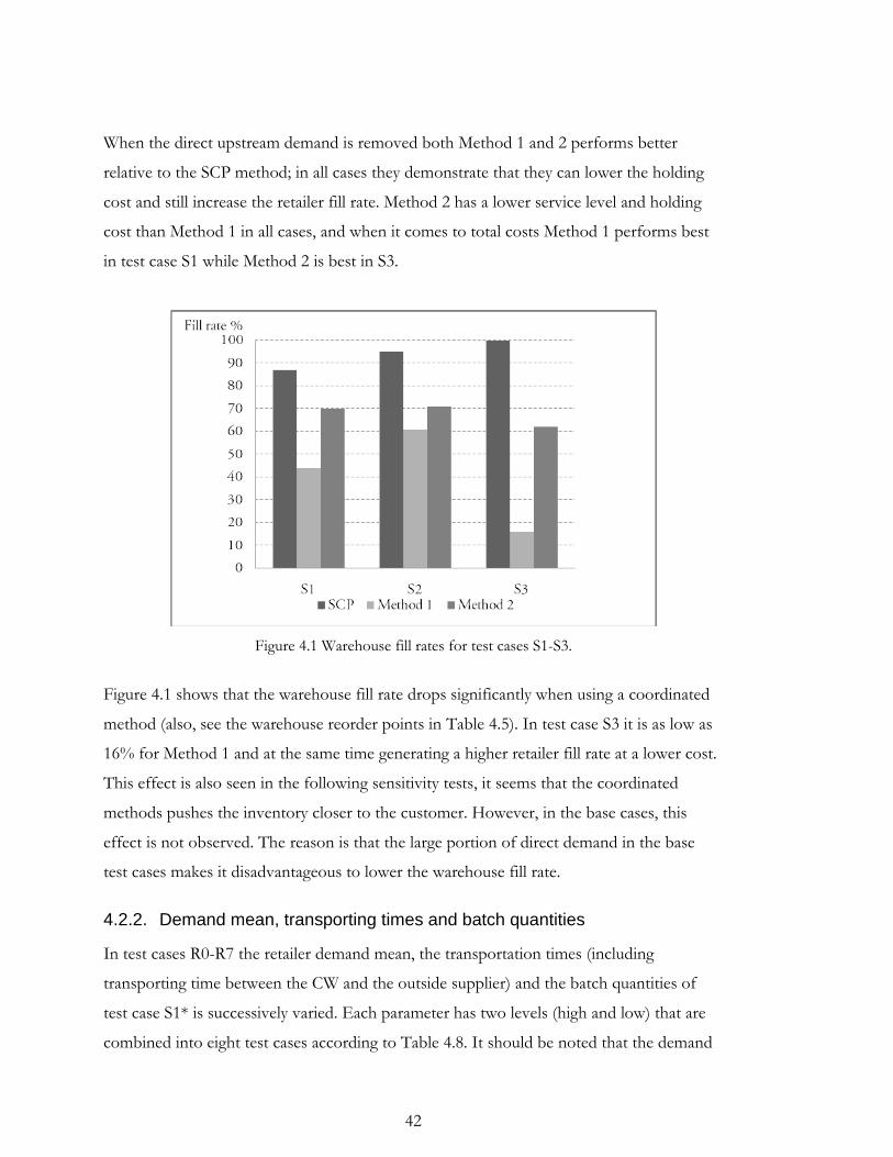
42

When the direct upstream demand is removed both Method 1 and 2 performs better

relative to the SCP method; in all cases they demonstrate that they can lower the holding

cost and still increase the retailer fill rate. Method 2 has a lower service level and holding

cost than Method 1 in all cases, and when it comes to total costs Method 1 performs best

in test case S1 while Method 2 is best in S3.

Figure 4.1 Warehouse fill rates for test cases S1-S3.

Figure 4.1 shows that the warehouse fill rate drops significantly when using a coordinated

method (also, see the warehouse reorder points in Table 4.5). In test case S3 it is as low as

16% for Method 1 and at the same time generating a higher retailer fill rate at a lower cost.

This effect is also seen in the following sensitivity tests, it seems that the coordinated

methods pushes the inventory closer to the customer. However, in the base cases, this

effect is not observed. The reason is that the large portion of direct demand in the base

test cases makes it disadvantageous to lower the warehouse fill rate.

4.2.2. Demand mean, transporting times and batch quantities

In test cases R0-R7 the retailer demand mean, the transportation times (including

transporting time between the CW and the outside supplier) and the batch quantities of

test case S1* is successively varied. Each parameter has two levels (high and low) that are

combined into eight test cases according to Table 4.8. It should be noted that the demand

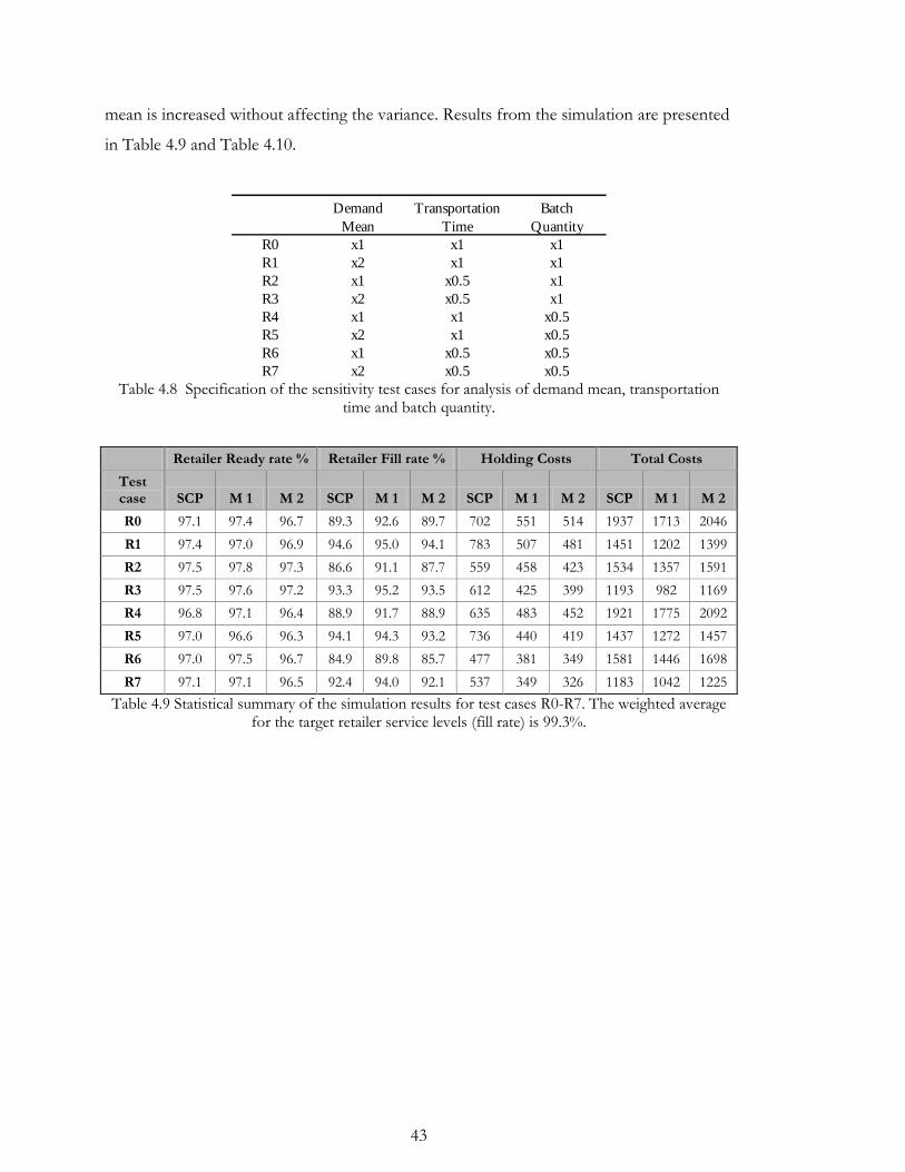
43

mean is increased without affecting the variance. Results from the simulation are presented

in Table 4.9 and Table 4.10.

Demand Transportation Batch

Mean Time Quantity

R0 x1 x1 x1

R1 x2 x1 x1

R2 x1 x0.5 x1

R3 x2 x0.5 x1

R4 x1 x1 x0.5

R5 x2 x1 x0.5

R6 x1 x0.5 x0.5

R7 x2 x0.5 x0.5 Table 4.8 Specification of the sensitivity test cases for analysis of demand mean, transportation

time and batch quantity.

Retailer Ready rate % Retailer Fill rate % Holding Costs Total Costs

Test case SCP M 1 M 2 SCP M 1 M 2 SCP M 1 M 2 SCP M 1 M 2

R0 97.1 97.4 96.7 89.3 92.6 89.7 702 551 514 1937 1713 2046

R1 97.4 97.0 96.9 94.6 95.0 94.1 783 507 481 1451 1202 1399

R2 97.5 97.8 97.3 86.6 91.1 87.7 559 458 423 1534 1357 1591

R3 97.5 97.6 97.2 93.3 95.2 93.5 612 425 399 1193 982 1169

R4 96.8 97.1 96.4 88.9 91.7 88.9 635 483 452 1921 1775 2092

R5 97.0 96.6 96.3 94.1 94.3 93.2 736 440 419 1437 1272 1457

R6 97.0 97.5 96.7 84.9 89.8 85.7 477 381 349 1581 1446 1698

R7 97.1 97.1 96.5 92.4 94.0 92.1 537 349 326 1183 1042 1225

Table 4.9 Statistical summary of the simulation results for test cases R0-R7. The weighted average for the target retailer service levels (fill rate) is 99.3%.

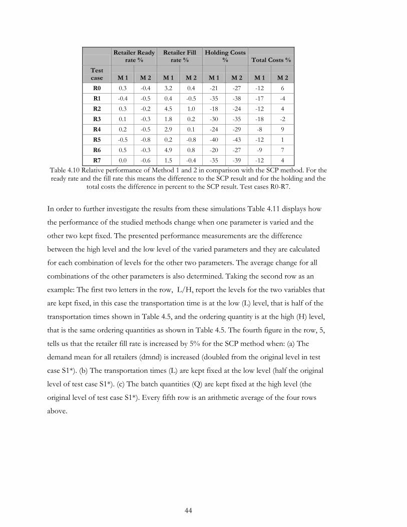
44

Retailer Ready

rate % Retailer Fill

rate % Holding Costs

% Total Costs %

Test case M 1 M 2 M 1 M 2 M 1 M 2 M 1 M 2

R0 0.3 -0.4 3.2 0.4 -21 -27 -12 6

R1 -0.4 -0.5 0.4 -0.5 -35 -38 -17 -4

R2 0.3 -0.2 4.5 1.0 -18 -24 -12 4

R3 0.1 -0.3 1.8 0.2 -30 -35 -18 -2

R4 0.2 -0.5 2.9 0.1 -24 -29 -8 9

R5 -0.5 -0.8 0.2 -0.8 -40 -43 -12 1

R6 0.5 -0.3 4.9 0.8 -20 -27 -9 7

R7 0.0 -0.6 1.5 -0.4 -35 -39 -12 4

Table 4.10 Relative performance of Method 1 and 2 in comparison with the SCP method. For the ready rate and the fill rate this means the difference to the SCP result and for the holding and the

total costs the difference in percent to the SCP result. Test cases R0-R7.

In order to further investigate the results from these simulations Table 4.11 displays how

the performance of the studied methods change when one parameter is varied and the

other two kept fixed. The presented performance measurements are the difference

between the high level and the low level of the varied parameters and they are calculated

for each combination of levels for the other two parameters. The average change for all

combinations of the other parameters is also determined. Taking the second row as an

example: The first two letters in the row, L/H, report the levels for the two variables that

are kept fixed, in this case the transportation time is at the low (L) level, that is half of the

transportation times shown in Table 4.5, and the ordering quantity is at the high (H) level,

that is the same ordering quantities as shown in Table 4.5. The fourth figure in the row, 5,

tells us that the retailer fill rate is increased by 5% for the SCP method when: (a) The

demand mean for all retailers (dmnd) is increased (doubled from the original level in test

case S1*). (b) The transportation times (L) are kept fixed at the low level (half the original

level of test case S1*). (c) The batch quantities (Q) are kept fixed at the high level (the

original level of test case S1*). Every fifth row is an arithmetic average of the four rows

above.

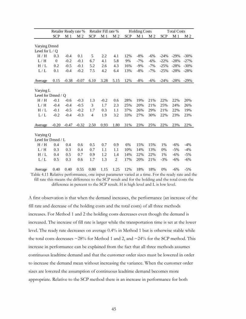
45

Retailer Ready rate % Retailer Fill rate % Holding Costs Total Costs

SCP M 1 M 2 SCP M 1 M 2 SCP M 1 M 2 SCP M 1 M 2

Varying Dmnd

Level for L / Q

H / H 0.3 -0.4 0.1 5 2.2 4.1 12% -8% -6% -24% -29% -30%

L / H 0 -0.2 -0.1 6.7 4.1 5.8 9% -7% -6% -22% -28% -27%

H / L 0.2 -0.5 -0.1 5.2 2.6 4.3 16% -9% -7% -25% -28% -30%

L / L 0.1 -0.4 -0.2 7.5 4.2 6.4 13% -8% -7% -25% -28% -28%

Average 0.15 -0.38 -0.07 6.10 3.28 5.15 12% -8% -6% -24% -28% -29%

Varying L

Level for Dmnd / Q

H / H -0.1 -0.6 -0.3 1.3 -0.2 0.6 28% 19% 21% 22% 22% 20%

L / H -0.4 -0.4 -0.5 3 1.7 2.3 25% 20% 21% 25% 24% 26%

H / L -0.1 -0.5 -0.2 1.7 0.3 1.1 37% 26% 29% 21% 22% 19%

L / L -0.2 -0.4 -0.3 4 1.9 3.2 33% 27% 30% 22% 23% 23%

Average -0.20 -0.47 -0.32 2.50 0.93 1.80 31% 23% 25% 22% 23% 22%

Varying Q

Level for Dmnd / L

H / H 0.4 0.4 0.6 0.5 0.7 0.9 6% 15% 15% 1% -6% -4%

L / H 0.3 0.3 0.4 0.7 1.1 1.1 10% 14% 13% 0% -5% -4%

H / L 0.4 0.5 0.7 0.9 1.2 1.4 14% 22% 22% 1% -6% -5%

L / L 0.5 0.3 0.6 1.7 1.3 2 17% 20% 21% -3% -6% -6%

Average 0.40 0.40 0.55 0.80 1.15 1.25 12% 18% 18% 0% -6% -5% Table 4.11 Relative performance, one input parameter varied at a time. For the ready rate and the

fill rate this means the difference to the SCP result and for the holding and the total costs the difference in percent to the SCP result. H is high level and L is low level.

A first observation is that when the demand increases, the performance (an increase of the

fill rate and decrease of the holding costs and the total costs) of all three methods

increases. For Method 1 and 2 the holding costs decreases even though the demand is

increased. The increase of fill rate is larger while the transportation time is set at the lower

level. The ready rate decreases on average 0.4% in Method 1 but is otherwise stable while

the total costs decreases ~28% for Method 1 and 2, and ~24% for the SCP method. This

increase in performance can be explained from the fact that all three methods assumes

continuous leadtime demand and that the customer order sizes must be lowered in order

to increase the demand mean without increasing the variance. When the customer order

sizes are lowered the assumption of continuous leadtime demand becomes more

appropriate. Relative to the SCP method there is an increase in performance for both

46

Method 1 and 2 when the demand increases for the fill rate, the holding costs and the total

costs.

An increase in the transportation times, L, yields a reduction in the ready rate for all

methods, with the largest reduction in Method 1. The fill rate increases for all methods and

the holding cost increases substantially, with a larger increase when the batch size is low.

The fill rate increase is largest for the SCP method and so is the increase in holding costs.

Total costs increases around 22% for all methods. Relative to the SCP method there is an

increase in performance for both Method 1 and 2 when the leadtime increases for the fill

rate and the holding costs.

When increasing the batch size, Q, an increase of the ready rate is observed for all

methods. The fill rate is also increased (~1%) for all methods with no significant

correlations with the other parameters. An increase is observed in the holding cost for all

methods (18% for Method 1 and 2, and 12% for the SCP method), this increase is

negatively correlated with both transportation time and demand mean. Despite this

increase in holding cost the total cost still decreases for Method 1 and 2 (~5%), no change

is observed for the SCP method. Relative to the SCP method there is an increase in

performance for both Method 1 and 2 when the batch size increases for the fill rate, the

holding costs and the total costs.

Turning to the performance of Method 1 and Method 2 when compared to the

performance of the SCP method (Table 4.10). The parameter with the most influence on

the fill rate and the holding costs is the demand mean. When the demand mean is

increased the relative fill rate is decreased somewhat and the holding costs are decreased

substantially. The same effect, but smaller, is indicated when the leadtime is increased. This

is not surprising since both these changes affects the leadtime demand. When increasing

the batch quantity, the fill rate is stable but the relative holding costs is increased to some

extent.

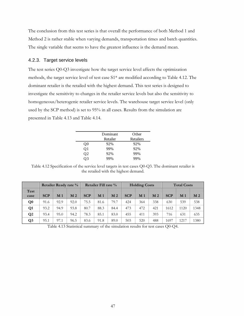
47

The conclusion from this test series is that overall the performance of both Method 1 and

Method 2 is rather stable when varying demands, transportation times and batch quantities.

The single variable that seems to have the greatest influence is the demand mean.

4.2.3. Target service levels

The test series Q0-Q3 investigate how the target service level affects the optimization

methods, the target service level of test case S1* are modified according to Table 4.12. The

dominant retailer is the retailed with the highest demand. This test series is designed to

investigate the sensitivity to changes in the retailer service levels but also the sensitivity to

homogeneous/heterogenic retailer service levels. The warehouse target service level (only

used by the SCP method) is set to 95% in all cases. Results from the simulation are

presented in Table 4.13 and Table 4.14.

Dominant Other

Retailer Retailers

Q0 92% 92%

Q1 99% 92%

Q2 92% 99%

Q3 99% 99%

Table 4.12 Specification of the service level targets in test cases Q0-Q3. The dominant retailer is the retailed with the highest demand.

Retailer Ready rate % Retailer Fill rate % Holding Costs Total Costs

Test case SCP M 1 M 2 SCP M 1 M 2 SCP M 1 M 2 SCP M 1 M 2

Q0 91.6 92.9 92.0 75.5 81.6 79.7 424 364 338 630 539 538

Q1 93.2 94.9 93.8 80.7 88.3 84.4 473 472 421 1612 1120 1348

Q2 93.4 95.0 94.2 78.3 85.1 83.0 455 411 393 716 631 635

Q3 95.1 97.1 96.5 83.6 91.8 89.0 503 520 488 1697 1217 1380

Table 4.13 Statistical summary of the simulation results for test cases Q0-Q4.

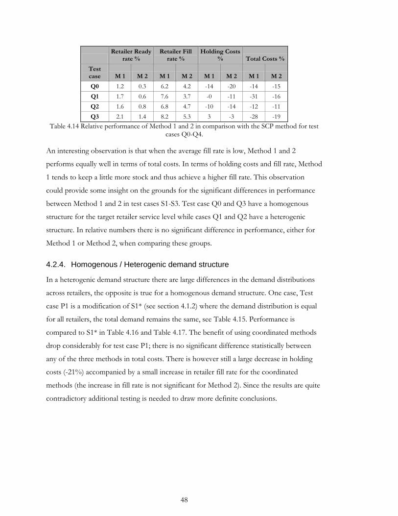
48

Retailer Ready

rate % Retailer Fill

rate % Holding Costs

% Total Costs %

Test case M 1 M 2 M 1 M 2 M 1 M 2 M 1 M 2

Q0 1.2 0.3 6.2 4.2 -14 -20 -14 -15

Q1 1.7 0.6 7.6 3.7 -0 -11 -31 -16

Q2 1.6 0.8 6.8 4.7 -10 -14 -12 -11

Q3 2.1 1.4 8.2 5.3 3 -3 -28 -19

Table 4.14 Relative performance of Method 1 and 2 in comparison with the SCP method for test cases Q0-Q4.

An interesting observation is that when the average fill rate is low, Method 1 and 2

performs equally well in terms of total costs. In terms of holding costs and fill rate, Method

1 tends to keep a little more stock and thus achieve a higher fill rate. This observation

could provide some insight on the grounds for the significant differences in performance

between Method 1 and 2 in test cases S1-S3. Test case Q0 and Q3 have a homogenous

structure for the target retailer service level while cases Q1 and Q2 have a heterogenic

structure. In relative numbers there is no significant difference in performance, either for

Method 1 or Method 2, when comparing these groups.

4.2.4. Homogenous / Heterogenic demand structure

In a heterogenic demand structure there are large differences in the demand distributions

across retailers, the opposite is true for a homogenous demand structure. One case, Test

case P1 is a modification of S1* (see section 4.1.2) where the demand distribution is equal

for all retailers, the total demand remains the same, see Table 4.15. Performance is

compared to S1* in Table 4.16 and Table 4.17. The benefit of using coordinated methods

drop considerably for test case P1; there is no significant difference statistically between

any of the three methods in total costs. There is however still a large decrease in holding

costs (-21%) accompanied by a small increase in retailer fill rate for the coordinated

methods (the increase in fill rate is not significant for Method 2). Since the results are quite

contradictory additional testing is needed to draw more definite conclusions.

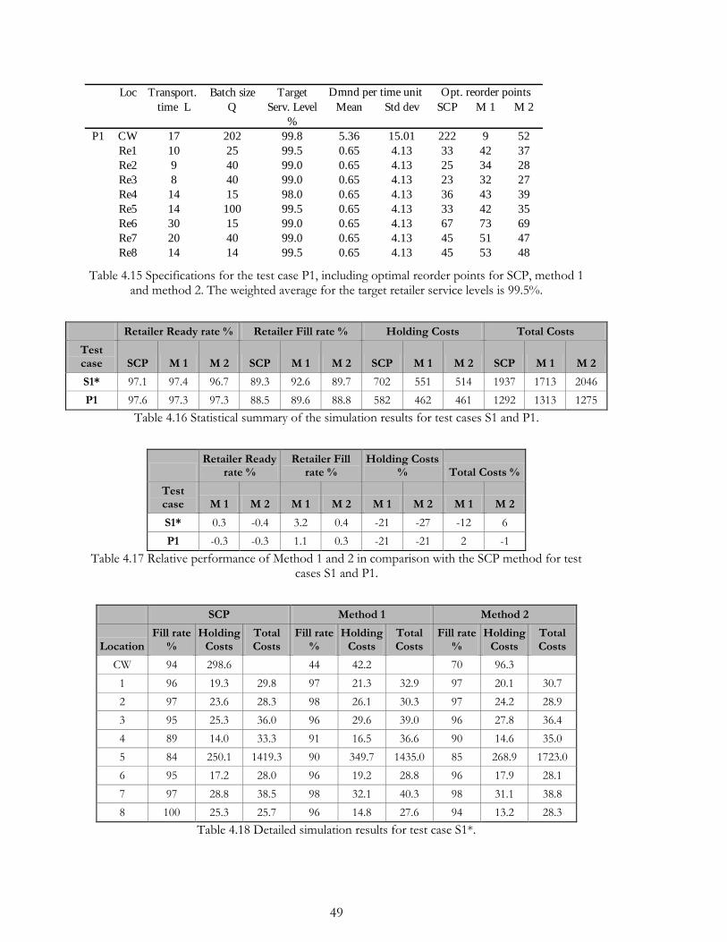
49

Loc Transport. Batch size Target

time L Q Serv. Level Mean Std dev SCP M 1 M 2

%

P1 CW 17 202 99.8 5.36 15.01 222 9 52

Re1 10 25 99.5 0.65 4.13 33 42 37

Re2 9 40 99.0 0.65 4.13 25 34 28

Re3 8 40 99.0 0.65 4.13 23 32 27

Re4 14 15 98.0 0.65 4.13 36 43 39

Re5 14 100 99.5 0.65 4.13 33 42 35

Re6 30 15 99.0 0.65 4.13 67 73 69

Re7 20 40 99.0 0.65 4.13 45 51 47

Re8 14 14 99.5 0.65 4.13 45 53 48

Dmnd per time unit Opt. reorder points

Table 4.15 Specifications for the test case P1, including optimal reorder points for SCP, method 1 and method 2. The weighted average for the target retailer service levels is 99.5%.

Retailer Ready rate % Retailer Fill rate % Holding Costs Total Costs

Test case SCP M 1 M 2 SCP M 1 M 2 SCP M 1 M 2 SCP M 1 M 2

S1* 97.1 97.4 96.7 89.3 92.6 89.7 702 551 514 1937 1713 2046

P1 97.6 97.3 97.3 88.5 89.6 88.8 582 462 461 1292 1313 1275

Table 4.16 Statistical summary of the simulation results for test cases S1 and P1.

Retailer Ready

rate % Retailer Fill

rate % Holding Costs

% Total Costs %

Test case M 1 M 2 M 1 M 2 M 1 M 2 M 1 M 2

S1* 0.3 -0.4 3.2 0.4 -21 -27 -12 6

P1 -0.3 -0.3 1.1 0.3 -21 -21 2 -1

Table 4.17 Relative performance of Method 1 and 2 in comparison with the SCP method for test cases S1 and P1.

SCP Method 1 Method 2

Location Fill rate

% Holding

Costs Total Costs

Fill rate %

Holding Costs

Total Costs

Fill rate %

Holding Costs

Total Costs

CW 94 298.6 44 42.2 70 96.3

1 96 19.3 29.8 97 21.3 32.9 97 20.1 30.7

2 97 23.6 28.3 98 26.1 30.3 97 24.2 28.9

3 95 25.3 36.0 96 29.6 39.0 96 27.8 36.4

4 89 14.0 33.3 91 16.5 36.6 90 14.6 35.0

5 84 250.1 1419.3 90 349.7 1435.0 85 268.9 1723.0

6 95 17.2 28.0 96 19.2 28.8 96 17.9 28.1

7 97 28.8 38.5 98 32.1 40.3 98 31.1 38.8

8 100 25.3 25.7 96 14.8 27.6 94 13.2 28.3

Table 4.18 Detailed simulation results for test case S1*.

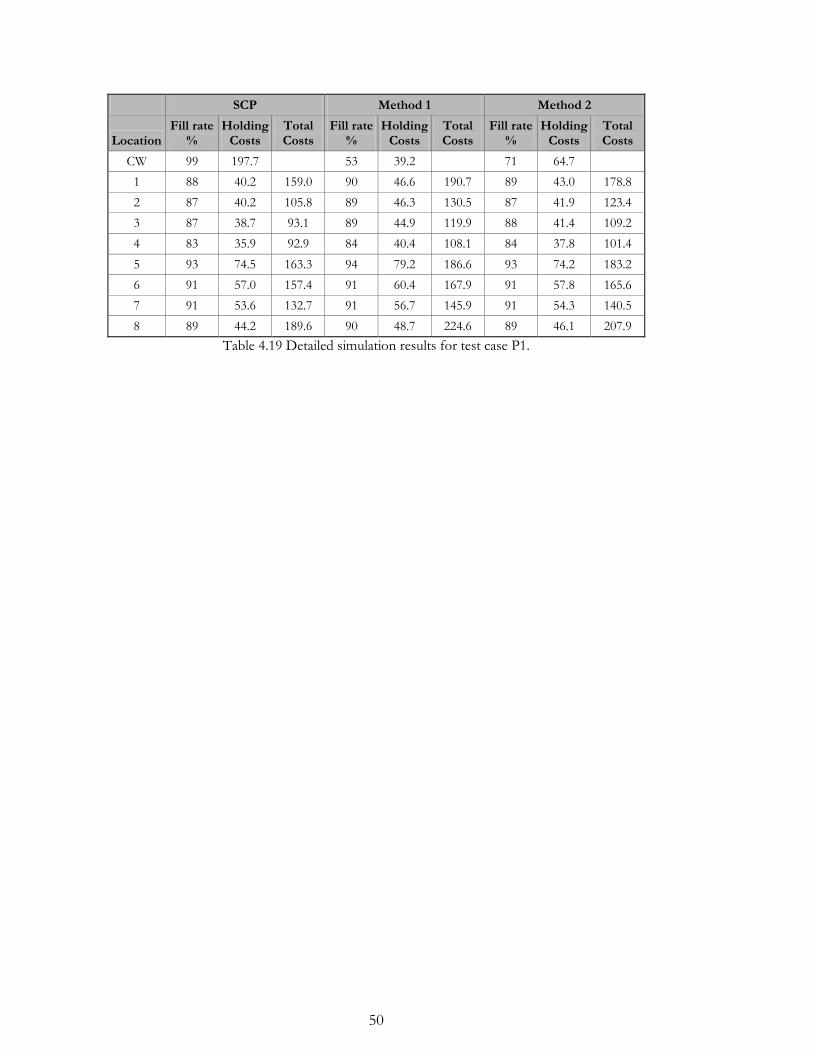
50

SCP Method 1 Method 2

Location Fill rate

% Holding

Costs Total Costs

Fill rate %

Holding Costs

Total Costs

Fill rate %

Holding Costs

Total Costs

CW 99 197.7 53 39.2 71 64.7

1 88 40.2 159.0 90 46.6 190.7 89 43.0 178.8

2 87 40.2 105.8 89 46.3 130.5 87 41.9 123.4

3 87 38.7 93.1 89 44.9 119.9 88 41.4 109.2

4 83 35.9 92.9 84 40.4 108.1 84 37.8 101.4

5 93 74.5 163.3 94 79.2 186.6 93 74.2 183.2

6 91 57.0 157.4 91 60.4 167.9 91 57.8 165.6

7 91 53.6 132.7 91 56.7 145.9 91 54.3 140.5

8 89 44.2 189.6 90 48.7 224.6 89 46.1 207.9

Table 4.19 Detailed simulation results for test case P1.

51

5. CONCLUSIONS AND FUTURE RESEARCH

The objective of this thesis is to expose newly developed methods for coordinated multi-

echelon control of inventory levels to real conditions and investigate the value of using

those in comparison with a widely used single stage (uncoordinated) method.

The simulation results clearly indicate that the evaluated methods for coordinated control

of inventories can offer considerable savings in reduced inventory levels and even, in many

cases, at the same time increasing the fill rate. When the direct upstream demand is

excluded the reductions in total cost range 11-37% and an increase in fill rate accompanied

by a reduction of the holding costs is observed in most cases. Especially the holding costs

at the Central Warehouse can be reduced, when using a method for coordinated control

the fill rate for orders from the retailers is 16-71% which corresponds to a reduction of the

CW holding costs of 50-94%. As expected, the benefits decrease when allowing for direct

upstream demand. Particularly Method 2 has difficulties in this case with increases of total

costs in all three cases, in one case as large as 111%. These results advise against using

Method 2 in cases of direct upstream demand. Method 1, which still achieves reductions in

total costs, seems to be more robust to large portions of direct upstream demand. A reason

for the poorer performance could be that the direct upstream demand makes it

disadvantageous to lower the CW fill rate.

Both Method 1 and Method 2 are quite robust to the changes in demand mean, leadtime

and batch size. Method 1 performs better when the target service levels are low (in relative

terms). Method 2 is more stable when target service levels are varied. The results are quite

contradictory when it comes to the effect of a homogenous or heterogenic demand

structure and additional testing is needed to draw general conclusions.

Apparent disadvantages of using coordinated control in a multi-echelon inventory system

is that it requires more data in one location to make the calculations, and that the

calculations is much more computationally demanding than for an uncoordinated method.

Depending on the size and level of demand in the system the computation time range 4 - 9

52

seconds for Method 1and 0.5 - 3 seconds for Method 2, on a computer equipped with an

Intel Pentium M 1.8 GHz processor.

Regarding future research it would be valuable to map out the limitations of the methods

more closely, to facilitate the process of applying the methods in situations they are verified

to produce satisfactory results in. It would also be interesting to investigate if and how the

methods can be adapted to handle direct upstream demand more effectively. If the

methods for coordinated control would be implemented in a commercial system it would

also be valuable to benchmark the computational requirements for the methods.

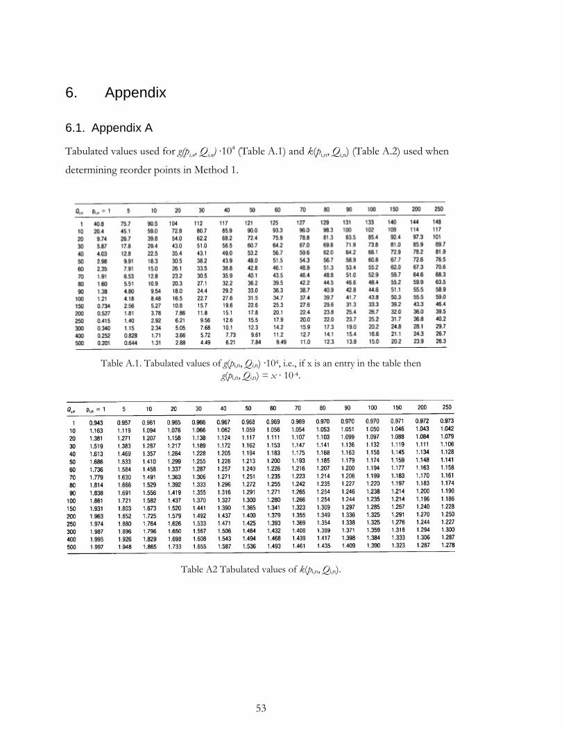
53

6. Appendix

6.1. Appendix A

Tabulated values used for g(pi,n, Qi,n) ∙104 (Table A.1) and k(pi,n, Qi,n) (Table A.2) used when

determining reorder points in Method 1.

Table A.1. Tabulated values of g(pi,n, Qi,n) ∙104, i.e., if x is an entry in the table then

g(pi,n, Qi,n) = x ∙ 10-4.

Table A2 Tabulated values of k(pi,n, Qi,n).

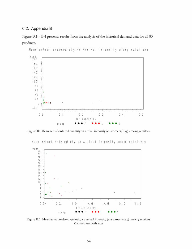
54

6.2. Appendix B

Figure B.1 – B.4 presents results from the analysis of the historical demand data for all 80

products.

Figure B1 Mean actual ordered quantity vs arrival intensity (customers/day) among retailers.

Figure B.2. Mean actual ordered quantity vs arrival intensity (customers/day) among retailers. Zoomed on both axes.

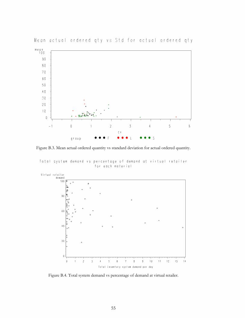
55

Figure B.3. Mean actual ordered quantity vs standard deviation for actual ordered quantity.

Figure B.4. Total system demand vs percentage of demand at virtual retailer.

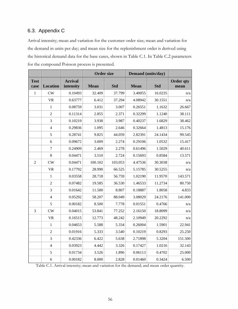
56

6.3. Appendix C

Arrival intensity; mean and variation for the customer order size; mean and variation for

the demand in units per day; and mean size for the replenishment order is derived using

the historical demand data for the base cases, shown in Table C.1. In Table C.2 parameters

for the compound Poisson process is presented.

Order size Demand (units/day)

Test

case Location

Arrival

intensity Mean Std Mean Std

Order qty

mean

1 CW 0.10493 32.409 37.799 3.40055 16.0235 n/a

VR 0.63777 6.412 37.294 4.08942 30.1551 n/a

1 0.08759 3.031 3.007 0.26551 1.1632 26.667

2 0.11314 2.855 2.371 0.32299 1.1240 38.111

3 0.10219 3.938 3.987 0.40237 1.6829 38.462

4 0.29836 1.095 2.646 0.32664 1.4813 15.176

5 0.28741 9.825 44.059 2.82391 24.1434 99.545

6 0.09672 3.009 2.274 0.29106 1.0532 15.417

7 0.24909 2.469 2.278 0.61496 1.5029 40.611

8 0.04471 3.510 2.724 0.15693 0.8584 13.571

2 CW 0.04471 100.102 103.053 4.47536 30.3038 n/a

VR 0.17792 28.990 66.525 5.15785 30.5255 n/a

1 0.03558 28.718 56.759 1.02190 11.9570 143.571

2 0.07482 19.585 36.530 1.46533 11.2734 80.750

3 0.01642 11.500 8.807 0.18887 1.8058 4.833

4 0.05292 58.207 88.049 3.08029 24.2176 141.000

5 0.00182 8.500 7.778 0.01551 0.4766 n/a

3 CW 0.04015 53.841 77.252 2.16150 18.8099 n/a

VR 0.16515 12.773 48.242 2.10949 20.2292 n/a

1 0.04653 5.588 5.334 0.26004 1.5901 22.941

2 0.01916 5.333 3.540 0.10219 0.8293 25.250

3 0.42336 6.422 5.638 2.71898 5.3204 151.500

4 0.03923 4.442 3.326 0.17427 1.0216 32.143

5 0.01734 3.526 1.896 0.06113 0.4702 25.000

6 0.00182 8.000 2.828 0.01460 0.3424 6.500

Table C.1. Arrival intensity; mean and variation for the demand; and mean order quantity.

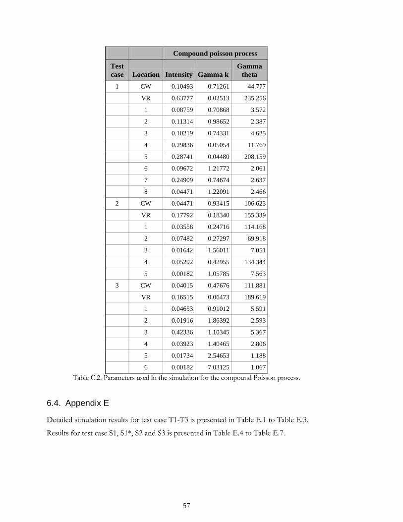
57

Compound poisson process

Test

case Location Intensity Gamma k

Gamma

theta

1 CW 0.10493 0.71261 44.777

VR 0.63777 0.02513 235.256

1 0.08759 0.70868 3.572

2 0.11314 0.98652 2.387

3 0.10219 0.74331 4.625

4 0.29836 0.05054 11.769

5 0.28741 0.04480 208.159

6 0.09672 1.21772 2.061

7 0.24909 0.74674 2.637

8 0.04471 1.22091 2.466

2 CW 0.04471 0.93415 106.623

VR 0.17792 0.18340 155.339

1 0.03558 0.24716 114.168

2 0.07482 0.27297 69.918

3 0.01642 1.56011 7.051

4 0.05292 0.42955 134.344

5 0.00182 1.05785 7.563

3 CW 0.04015 0.47676 111.881

VR 0.16515 0.06473 189.619

1 0.04653 0.91012 5.591

2 0.01916 1.86392 2.593

3 0.42336 1.10345 5.367

4 0.03923 1.40465 2.806

5 0.01734 2.54653 1.188

6 0.00182 7.03125 1.067

Table C.2. Parameters used in the simulation for the compound Poisson process.

6.4. Appendix E

Detailed simulation results for test case T1-T3 is presented in Table E.1 to Table E.3.

Results for test case S1, S1*, S2 and S3 is presented in Table E.4 to Table E.7.

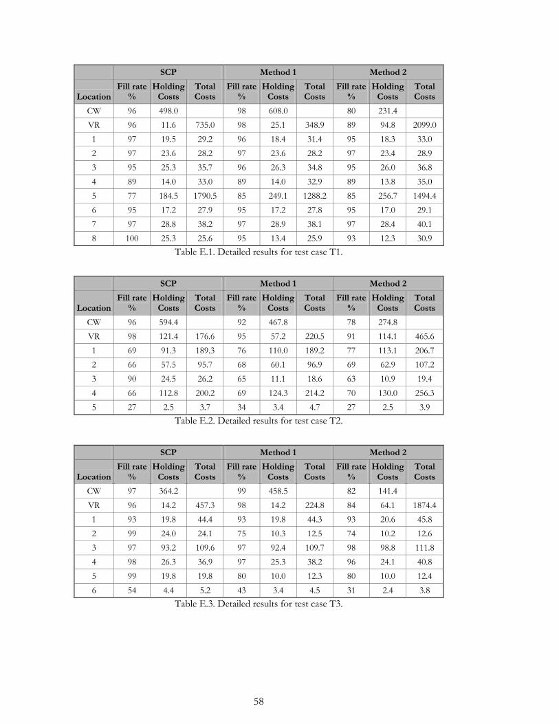
58

SCP Method 1 Method 2

Location Fill rate

% Holding

Costs Total Costs

Fill rate %

Holding Costs

Total Costs

Fill rate %

Holding Costs

Total Costs

CW 96 498.0 98 608.0 80 231.4

VR 96 11.6 735.0 98 25.1 348.9 89 94.8 2099.0

1 97 19.5 29.2 96 18.4 31.4 95 18.3 33.0

2 97 23.6 28.2 97 23.6 28.2 97 23.4 28.9

3 95 25.3 35.7 96 26.3 34.8 95 26.0 36.8

4 89 14.0 33.0 89 14.0 32.9 89 13.8 35.0

5 77 184.5 1790.5 85 249.1 1288.2 85 256.7 1494.4

6 95 17.2 27.9 95 17.2 27.8 95 17.0 29.1

7 97 28.8 38.2 97 28.9 38.1 97 28.4 40.1

8 100 25.3 25.6 95 13.4 25.9 93 12.3 30.9

Table E.1. Detailed results for test case T1.

SCP Method 1 Method 2

Location Fill rate

% Holding

Costs Total Costs

Fill rate %

Holding Costs

Total Costs

Fill rate %

Holding Costs

Total Costs

CW 96 594.4 92 467.8 78 274.8

VR 98 121.4 176.6 95 57.2 220.5 91 114.1 465.6

1 69 91.3 189.3 76 110.0 189.2 77 113.1 206.7

2 66 57.5 95.7 68 60.1 96.9 69 62.9 107.2

3 90 24.5 26.2 65 11.1 18.6 63 10.9 19.4

4 66 112.8 200.2 69 124.3 214.2 70 130.0 256.3

5 27 2.5 3.7 34 3.4 4.7 27 2.5 3.9

Table E.2. Detailed results for test case T2.

SCP Method 1 Method 2

Location Fill rate

% Holding

Costs Total Costs

Fill rate %

Holding Costs

Total Costs

Fill rate %

Holding Costs

Total Costs

CW 97 364.2 99 458.5 82 141.4

VR 96 14.2 457.3 98 14.2 224.8 84 64.1 1874.4

1 93 19.8 44.4 93 19.8 44.3 93 20.6 45.8

2 99 24.0 24.1 75 10.3 12.5 74 10.2 12.6

3 97 93.2 109.6 97 92.4 109.7 98 98.8 111.8

4 98 26.3 36.9 97 25.3 38.2 96 24.1 40.8

5 99 19.8 19.8 80 10.0 12.3 80 10.0 12.4

6 54 4.4 5.2 43 3.4 4.5 31 2.4 3.8

Table E.3. Detailed results for test case T3.

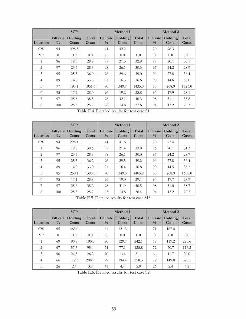
59

SCP Method 1 Method 2

Location Fill rate

% Holding

Costs Total Costs

Fill rate %

Holding Costs

Total Costs

Fill rate %

Holding Costs

Total Costs

CW 94 298.5 44 42.2 70 96.3

VR 0 0.0 0.0 0 0.0 0.0 0 0.0 0.0

1 96 19.3 29.8 97 21.3 32.9 97 20.1 30.7

2 97 23.6 28.3 98 26.1 30.3 97 24.2 28.9

3 95 25.3 36.0 96 29.6 39.0 96 27.8 36.4

4 89 14.0 33.3 91 16.5 36.6 90 14.6 35.0

5 77 183.1 1951.6 90 349.7 1435.0 85 268.9 1723.0

6 95 17.2 28.0 96 19.2 28.8 96 17.9 28.1

7 97 28.8 38.5 98 32.1 40.3 98 31.1 38.8

8 100 25.3 25.7 96 14.8 27.6 94 13.2 28.3

Table E.4. Detailed results for test case S1.

SCP Method 1 Method 2

Location Fill rate

% Holding

Costs Total Costs

Fill rate %

Holding Costs

Total Costs

Fill rate %

Holding Costs

Total Costs

CW 94 298.1 44 41.6 70 95.4

1 96 19.3 30.6 97 21.4 33.8 96 20.1 31.3

2 97 23.5 28.3 98 26.1 30.0 97 24.2 28.7

3 95 25.3 36.2 96 29.5 39.2 96 27.8 36.4

4 89 14.0 33.0 91 16.4 36.8 90 14.5 35.3

5 85 250.1 1395.3 90 349.5 1405.9 85 268.9 1688.0

6 95 17.1 28.8 96 19.0 29.1 95 17.7 28.9

7 97 28.6 38.2 98 31.9 40.5 98 31.0 38.7

8 100 25.3 25.7 95 14.8 28.4 94 13.2 29.2

Table E.5. Detailed results for test case S1*.

SCP Method 1 Method 2

Location Fill rate

% Holding

Costs Total Costs

Fill rate %

Holding Costs

Total Costs

Fill rate %

Holding Costs

Total Costs

CW 95 463.0 61 121.3 71 167.0

VR 0 0.0 0.0 0 0.0 0.0 0 0.0 0.0

1 69 90.8 190.0 80 129.7 242.1 78 119.2 225.6

2 67 57.5 95.4 74 77.1 125.8 72 70.7 116.3

3 90 24.5 26.2 70 13.4 21.1 66 11.7 20.0

4 66 112.3 208.9 79 194.4 358.3 72 149.8 325.5

5 26 2.4 3.8 41 4.4 5.9 26 2.4 4.2

Table E.6. Detailed results for test case S2.

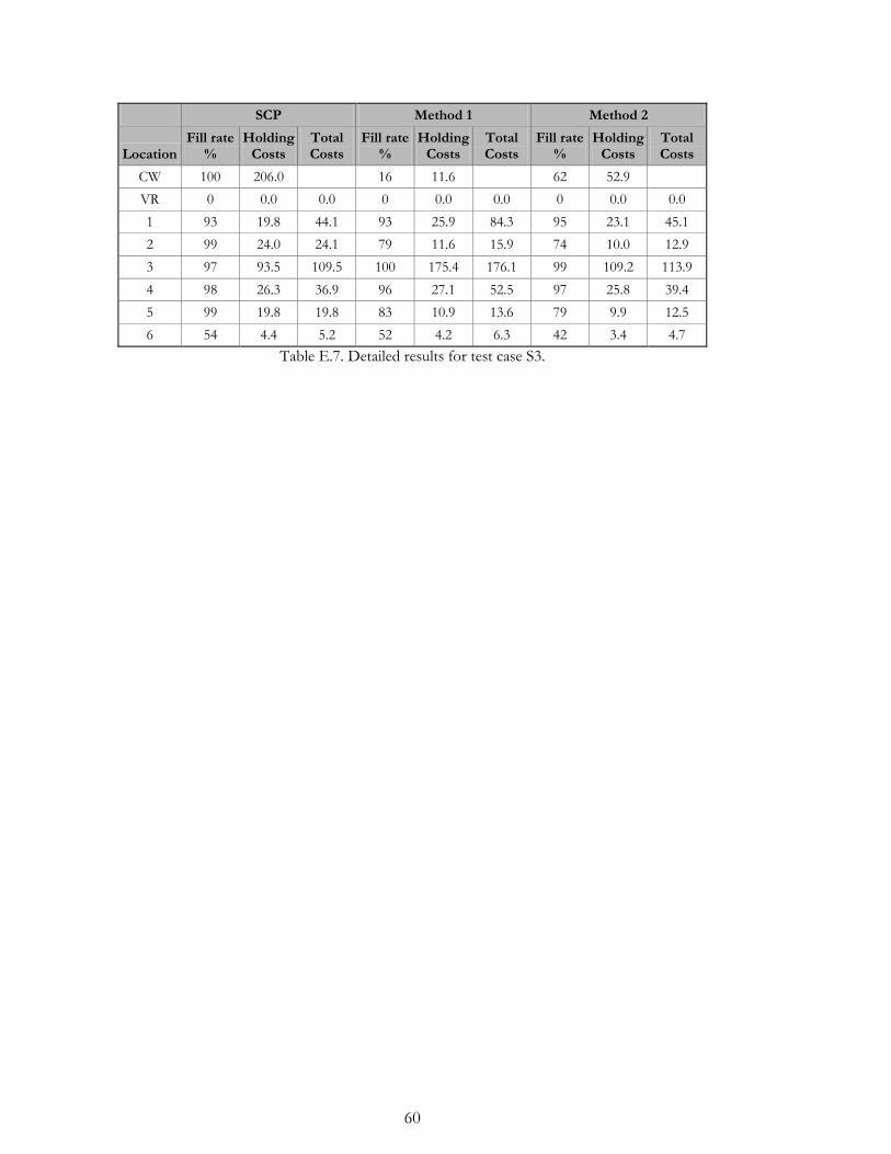
60

SCP Method 1 Method 2

Location Fill rate

% Holding

Costs Total Costs

Fill rate %

Holding Costs

Total Costs

Fill rate %

Holding Costs

Total Costs

CW 100 206.0 16 11.6 62 52.9

VR 0 0.0 0.0 0 0.0 0.0 0 0.0 0.0

1 93 19.8 44.1 93 25.9 84.3 95 23.1 45.1

2 99 24.0 24.1 79 11.6 15.9 74 10.0 12.9

3 97 93.5 109.5 100 175.4 176.1 99 109.2 113.9

4 98 26.3 36.9 96 27.1 52.5 97 25.8 39.4

5 99 19.8 19.8 83 10.9 13.6 79 9.9 12.5

6 54 4.4 5.2 52 4.2 6.3 42 3.4 4.7

Table E.7. Detailed results for test case S3.

61

References

Andersson, J., Axsäter, S., Marklund, J., 1998. Decentralized multiechelon

inventory control. Production and Operations Management 7(4) 370-386.

Andersson, J., Marklund, J., 2000. Decentralised inventory control in a two-level

distribution system. European Journal of Operations Research 127, 483-506.

Axsäter, S., 1991. Lagerstyrning, Studentlitteratur AB.

Axsäter, S., 1996. Using the deterministic EOQ formula in stochastic inventory

control. Management Science 42, 830-834.

Axsäter, S., 2000. Inventory Control. Kluwer Academic Publishers, Boston.

Axsäter, S., 2003. Approximate optimization of a two-level distribution inventory system.

International Journal of Production Economics 81-82, 545-553.

Axsäter, S., 2006. Inventory Control, Springer-Verlag New York Inc.

Axsäter, S., Olsson, F., Tydesjö, P., 2007. Heuristics for handling direct

upstream demand in two-echelon distribution systems. International Journal of

Production Economics 108 (2007) 266-270.

Berling, B., Marklund, J., 2006. Heuristic coordination of decentralized inventory

system using induced backorder costs. Production and Operations Management 15(2)

294-310.

Blom, G., Holmquist, B., 1998. Statistikteori med tillämpningar. Studentlitteratur.

D'Agostino, R.B., Stephens, M.A, 1986. Goodness-of-fit techniques. CRC Press.

62

Morse, P.M., Kimball, G.E., Gass, S.I., 2003. Methods of Operational research. Courier Dover

Publications.

Howard, C., 2007. Myopic Allocation in Two-level Distribution Systems with Continuous

Review and Time Based Dispatching. Department of Mathematics, Linköping University.

Van Houtum, G.J, Inderfurth, K., Zijm W.H.M., 1996. Materials coordination in stochastic

multi-echelon systems. European Journal of Operational Research 95, 1-23

Zheng, Y.S., 1992. On properties of stochastic inventory systems. Management Science 38, 87-

103.