Three Generic Methods for Evaluating Stochastic Multi-Echelon

Inventory Systems ∗

David Simchi-Levi† and Yao Zhao‡

First draft March 2006, revised August 2006, May 2007

Abstract

Globalization, product proliferation and fast product innovation have significantly increased

the complexities of supply chains in many industries. One of the most important advancements

of supply chain management in recent years is the development of models and methodologies

for controlling inventory in general supply networks under uncertainty, and their wide-spread

applications to industry. These developments are based on three generic methods: the queueing-

inventory method, the lead-time demand method and the flow-unit method. In this paper, we

compare and contrast these methods by discussing their differences and connections, and showing

how to apply them systematically to characterize and evaluate various network topologies with

different supply processes, inventory policies and demand processes. Our objective is to forge

links among research strands on various network topologies and to develop unified methodologies.

Key words: Inventory control, multi-echelon, stochastic, policy evaluation, supply chain.

1 Introduction

Many real-world supply chains, such as those found in automotive, electronics, and consumer

packaged goods industries, consist of large-scale assembly and distribution operations with geo-

graphically dispersed facilities. Clearly, many of these supply chains support the production and

∗Due to the space limit, we have to make painful decisions on material selection while strive to maintain theintegrity of the paper. Any comments and suggestions are welcome.

†The Engineering Systems Division and the Department of Civil and Environmental Engineering, MassachusettsInstitute of Technology, Cambridge, MA

‡Department of Management Science and Information Systems, Rutgers University, Newark, NJ

1

2

distribution of multiple end-products which are assembled from hundreds or thousands of sub-

systems and components with widely varying lead times and costs.

One challenge in all these supply chains is the efficient management of inventory in a complex

network of facilities and products with stochastic demand, random supply and high inventory and

transportation costs. This requires one to specify the inventory policy for each product at each

facility so as to minimize the system-wide inventory cost subject to customer service requirements.

For many years both practitioners and academicians have recognized the potential benefit of effec-

tive inventory control in such networks. In fact, the literature on multi-echelon inventory control

can be dated back to the 1950s. However, it is only in the last few years that some of these benefits

have been realized, see, e.g., Lee and Billington (1993), Graves and Willems (2000) and Lin, et al.

(2000). Three reasons have contributed to this trend:

1. The availability of data, not only on network structure and bill of materials (BOM), but also

on demand processes, transportation lead times and manufacturing cycle times, etc.;

2. Industry is searching for scientific methods for inventory management that help to cope with

long lead times and the increase in customer service expectations.

3. Recent developments in modeling and algorithms for the control of general structure multi-

echelon inventory systems;

These developments are built on three generic methods: the queueing-inventory method, the

lead-time demand method and the flow-unit method. While the first two methods take a snapshot

of the system and focus on quantities (e.g., backorders and on-hand inventory), the third method

follows the movement of each flow unit and focuses on times (e.g., stockout delays and inventory

holding times). This paper discusses the differences and connections among these methods, and

demonstrates their abilities in handling various network topologies, inventory policies and demand

processes.

1.1 Classification of Literature

To position our survey in perspective, we classify the related literature by several dimensions.

Models with zero lead times vs. Models with positive lead times. Models with zero lead

times can be used to analyze strategic issues as well as tactical or operational issues when the

3

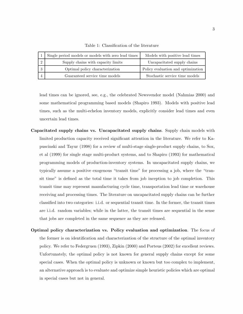
Table 1: Classification of the literature

1 Single period models or models with zero lead times Models with positive lead times

2 Supply chains with capacity limits Uncapacitated supply chains

3 Optimal policy characterization Policy evaluation and optimization

4 Guaranteed service time models Stochastic service time models

lead times can be ignored, see, e.g., the celebrated Newsvendor model (Nahmias 2000) and

some mathematical programming based models (Shapiro 1993). Models with positive lead

times, such as the multi-echelon inventory models, explicitly consider lead times and even

uncertain lead times.

Capacitated supply chains vs. Uncapacitated supply chains. Supply chain models with

limited production capacity received significant attention in the literature. We refer to Ka-

puscinski and Tayur (1998) for a review of multi-stage single-product supply chains, to Sox,

et al (1999) for single stage multi-product systems, and to Shapiro (1993) for mathematical

programming models of production-inventory systems. In uncapacitated supply chains, we

typically assume a positive exogenous “transit time” for processing a job, where the “tran-

sit time” is defined as the total time it takes from job inception to job completion. This

transit time may represent manufacturing cycle time, transportation lead time or warehouse

receiving and processing times. The literature on uncapacitated supply chains can be further

classified into two categories: i.i.d. or sequential transit time. In the former, the transit times

are i.i.d. random variables; while in the latter, the transit times are sequential in the sense

that jobs are completed in the same sequence as they are released.

Optimal policy characterization vs. Policy evaluation and optimization. The focus of

the former is on identification and characterization of the structure of the optimal inventory

policy. We refer to Federgruen (1993), Zipkin (2000) and Porteus (2002) for excellent reviews.

Unfortunately, the optimal policy is not known for general supply chains except for some

special cases. When the optimal policy is unknown or known but too complex to implement,

an alternative approach is to evaluate and optimize simple heuristic policies which are optimal

in special cases but not in general.

4

Guaranteed service time model vs. Stochastic service time model. In the former, it is

assumed that in case of stockout, each stage has resources other than the on-hand inventory

(such as slack capacity, expediting, etc.) to satisfy demand so that the committed service

times can always be guaranteed. In the latter, it is assumed that in case of stockout, each

stage fully backorders the unsatisfied demand and fills the demand until on-hand inventory

becomes available. Thus, the delay due to stockout (i.e., the stockout delay) is random and

the committed service times cannot be 100% guaranteed. A recent comparison between the

two models is provided by Graves and Willems (2003).

1.2 The Scope and Objective of the Survey

This survey focuses on the stochastic service time model for uncapacitated supply chains. Because

we are interested in general supply networks, we focus on policy evaluation and optimization. Given

a certain class of simple but effective inventory policies, the specific problem that we address in this

survey is how to characterize and evaluate system performance in general structure supply chains.

The challenge arises from the fact that the inventory policy controlling one product at one facility

may have an impact on all other products/facilities in the network either directly or indirectly.

For guaranteed service time models, Graves and Willems (2003) summarizes recent development

and demonstrates its potential applications in industry-size problems. These developments are

based on the lead-time demand method. For the stochastic service time model, Hadley and Whitin

(1963) provides the first comprehensive review for single-stage systems. Chen (1998b) reviews the

lead-time demand method in serial supply chains, and de Kok and Fransoo (2003) discusses some

of its applications in more general supply chains. Song and Zipkin (2003) provides an indepth

review of the literature on assembly systems, while Axsater (2003) presents an excellent survey

for serial and distribution systems. Zipkin (2000) presents an excellent and comprehensive review

for the queueing-inventory method in single-stage systems, and the lead-time demand method in

single-stage, serial, pure distribution and pure assembly systems.

The objective of this paper is to compare and contrast the queueing-inventory method, the

lead-time demand method and the flow-unit method along the following dimensions: network

topology, inventory policy and demand process. Specifically, we discuss how to apply each method

systematically to evaluate various network topologies with either i.i.d. or sequential transit times,

either base stock or batch ordering inventory policy and either unit or batch demand process. The

5

network topology considered includes single-stage (see Section §2), serial (§3.1), pure distribution

(§3.2), pure assembly and 2-level general networks (§3.3), tree and more general networks (§3.4).

For each network topology, we discuss the three methods side-by-side and address questions such

as, how are different stages connected and dependent? What are the key observations underlying

each method? How are the results/methods connected to those of single-stage systems and systems

of other topologies? And what are the differences and connections among the methods? Some open

questions are summarized in §4.

While some of the materials covered here appeared in previous reviews, we present these ma-

terials (together with recent results) in a coherent way by building connections among different

methods and establishing uniform treatment of each method across different network topologies.

We also shed some lights on the strengths and limitations of each method.

2 Single-Stage Systems

In this section, we consider single-stage systems and review the key assumptions and results of the

three generic methods. We show how each method can handle different inventory policies, transit

times and demand processes. Following convention, we define a stage (a node, equivalently) to be

a unique combination of a facility and a product, where the facility refers to a processor plus a

storage where the latter carries inventory processed by the former.

Inventory Policies. In this paper, we focus on either continuous-review or periodic-review base-

stock and batch ordering policies. For any stage in a supply chain, define inventory position to be

the sum of its on-hand inventory and outstanding orders subtracting backorders. Under continuous

review, a base-stock policy with base-stock level s works as follows: whenever inventory position

drops below s, order up to s. A batch ordering policy with reorder point r and batch size Q works

as follows: whenever the inventory position drops to or below the reorder point r, an order of size

nQ is placed to raise the inventory position up to the smallest integer above r. Clearly, a base-stock

policy is a special case of the batch-ordering policy with a batch size Q = 1. Continuous-review

base-stock policies are often used for expensive products facing low volume but highly uncertain

demand (e.g., service parts). Batch ordering policies are often used where economies of scale in

production and transportation cannot be ignored (commodities).

Under periodic review, the base-stock and batch ordering policies work in similar ways as their

6

continuous-review counterparts except that inventory is reviewed only once in one period. The

sequence of events is as follows (Hadley and Whitin 1963): At the beginning of a review period, the

replenishment is received, the inventory is reviewed and then an order decision is made. Demand

arrives during the period. At the end of the period, costs are calculated. Some work in the literature

assumes that all demand arrive at the end of the period; see, e.g., Zipkin (2000) Chapter 9. Under

this assumption, a single-stage periodic-review inventory system can be viewed as a special case

of its continuous-review counterpart with constant demand interarrival times and batch demand

sizes. In this survey, we assume demand arrives during the period unless otherwise mentioned.

Transit Times. If the transit times (§1.1) are sequential and stochastic, namely, “stochastic

sequential transit times”, then they must be dependent over consecutive orders. Kaplan (1970)

presents a discrete-time model for the stochastic sequential transit time in a periodic-review single-

stage system, where the evolution of the outstanding order vector is modeled by a Markov Chain.

See Song and Zipkin (1996) for a generalization of the model. For continuous-review single-stage

systems, Zipkin (1986) presents a continuous-time model for stochastic and sequential transit times.

Definition 2.1 The exogenous, stochastic and sequential transit times are defined as follows: thereexits an exogenous continuous-time stochastic process {U(t)} that is stationary and ergodic withfinite limiting moments, such that the sample path of {U(t)} is left-continuous, the transit time att, L(t) = U(t), and t+ L(t) is non-decreasing.

Svoronos and Zipkin (1991) applies this model to multi-stage supply chain with two additional

assumptions: (1) the transit times are independent of the system state, e.g., demand and order

placement, (2) the transit times are independent across stages.

In practice, the transit times can be either parallel or sequential or somewhere in between.

Many production and transportation processes in the real world are subject to random exogenous

events. Indeed, the orders placed by the systems under consideration may be a negligible portion

of their total workload. Thus, the transit times are exogenous and should be estimated from data.

While in some practical cases, the sequential transit time model may be more realistic than the

i.i.d. transit time model (Svoronos and Zipkin 1991), in cases such as repairing and maintenance,

the i.i.d. transit time model may be a better approximation (Sherbrooke 1968).

Demand Processes. Both unit demand and batch demand processes are studied in the literature.

On arrival of a batch demand, one shall address questions such as: should all units of the demand

7

be satisfied together (unsplit demand)? Or should each demand unit be satisfied separately (split

demand)? For a supply system (either production or transportation) processing a job of multiple

units, one needs to address questions like: is the job processed and replenished as an individable

entity (unsplit supply)? Or is each unit processed and replenished separately (split supply)? If the

former is true, does the transit time depend on job size? See Zipkin (2000) for more discussions on

these questions. While the case of split demand is easier to handle and thus widely studied in the

literature, the case of unsplit demand is much more difficult; see §2.1 for more details.

The Basic Assumption. For the ease of exposition, we make the following assumption throughout

the survey unless otherwise mentioned.

Assumption 2.2 The system is under continuous review; unsatisfied demand are fully backordered;outside suppliers have ample stock; the transit times are exogenous either i.i.d. or sequential;demand is satisfied on a first-come first-serve (FCFS) basis; demand can be split; supply cannot besplit and transit times do not depend on job sizes.

Throughout the survey, we use the following notations: a+ = max{a, 0}, a− = max{−a, 0}.E(·), V (·) are the mean and variance of a random variable, respectively. If random variables X

and Y are independent, we denote X ⊥ Y . We consider base-stock policies with s ≥ 0 and batch

ordering policies with r ≥ 0 unless otherwise mentioned.

We define the basic model for single-stage systems as follows: inventory is controlled by a base-

stock policy, demand follows Poisson process with rate λ, and the transit time (i.e., lead time) L is

constant. In the following subsections, we first discuss the methods in the basic model, and then

extend the results to more general demand process, inventory policies and supply process.

2.1 The Queueing-Inventory Method

Let {IO(t), t ≥ 0} be the outstanding order process, {IP (t), t ≥ 0} be the inventory position

process, and {IL(t), t ≥ 0} be the process of net inventory (on-hand minus backorder). Define

{I(t), t ≥ 0} ({B(t), t ≥ 0}) to be the process of on-hand inventory (backorder, respectively). For

appropriate initial conditions, the following conservation equation holds under Assumption 2.2,

IO(t) + IL(t) = IP (t), t ≥ 0, (1)

I(t) = IL(t)+, (2)

B(t) = IL(t)−. (3)

8

For unsplit demand, Eqs. (2)-(3) do not hold since I(t) > 0 and B(t) > 0 can hold simultaneously.

Note that IO(t) is the number of jobs in the supply process. The queueing-inventory method

characterizes the probability distribution of IO(t) by identifying the appropriate queueing analogue.

One can follow a 3-step procedure to characterize the system performance: (1) the distribution of

IP (t), (2) the distribution of IO(t), and (3) the dependence of IO(t) and IP (t). We focus on

steady-state analysis, and define IO = limt→∞ IO(t). The same notational rule applies to IL, IP

and I and B.

Clearly, IP = s for base-stock policies. For batch ordering policies, the distribution of IP only

depends on the demand process. IP is uniformly distributed in {r+1, r+2, . . . , r+Q} for renewal

batch demand under mild regularity assumptions (Sahin 1979). See Zipkin (1986) for a discussion

of more general demand processes. The distribution of IO depends on the demand process, the

inventory policy and the supply system (see discussions below). For batch ordering policies, IP

depends on IO. Intuitively, the lower the IP , the longer the time since the last order, and therefore

the lower the IO.

i.i.d. Transit Time. Consider first the basic model with constant L, the queueing analogue

is a M/D/∞ queue. By Palm theorem (Palm 1938), IO follows Poisson(λL) distribution. If

L is stochastic, then the queueing analogue is a M/G/∞ queue and IO follows Poisson(λE(L))

distribution. Because demand is satisfied on a FCFS basis, the stockout delay differs from L even at

s = 0; see Muckstadt (2004, page 96) for an exact analysis. For renewal unit demand, the queueing

analogue is a G/G/∞ queue. For compound Poisson demand, then the queueing analogue is a

MY /G/∞ queue where {Yn} is the demand size process. The distribution of IO is compound

Poisson under Assumption 2.2.

Consider the basic model but with a batch ordering policy, the queueing analogue is aErQ/D/∞queue where Er stands for Erlang interarrival times. See Galliher, Morse and Simond (1959) for

an exact analysis. For batch demand processes, tractable approximations become appealing. One

can first assume IP ⊥ IO, and then approximate the distribution of IO by results from systems

with base-stock policy and batch demand processes (Zipkin 2000, §7.2.4).

Sequential Transit Time. Consider the basic model with sequential transit times (Definition

2.1). Let D(t1, t2] be the demand during time interval (t1, t2] where t1 ≤ t2, and let D(∞|L] =

limt→∞D(t− L, t]. By Svoronos and Zipkin (1991),

9

Proposition 2.3 IO has the same distribution as D(∞|L].

Proof. See Appendix for a proof.

D(t − L, t] (D(∞|L]) is called the lead-time demand. If demand follows compound Poisson

process, Proposition 2.3 also holds under Assumption 2.2.

For the basic model with constant transit time, one can obtain Proposition 2.3 by an alternative

approach (Zipkin 2000). At time t, because all orders placed on or before t−L is replenished while

all orders placed after t−L are still in transit, IO(t) equals to the number of orders placed during

(t−L, t]. Due to the Poisson demand and the continuous-review base-stock policy, one must have,

IO(t) = D(t− L, t]. (4)

Consider the batch ordering policy in the basic model with sequential transit times (Definition

2.1). Eq. (4) does not hold because IO(t) is clearly not the demand during (t− L, t]. In addition,

IO(t) depends on IP (t). Exact analysis of these systems using the queueing-inventory method is

rare. Fortunately, such systems can be easily handled by the lead-time demand method and the

flow-unit method.

2.2 The Lead-Time Demand Method

Consider the basic model. Observe that at time t, the system receives all orders placed on or before

t− L but none of the orders placed after t− L, then,

IL(t) = IP (t− L) −D(t− L, t]. (5)

Eqs. (2)-(3) remain true here. Although Eq. (5) looks quite similar to Eqs. (1) and (4), they

follow completely different logic. Indeed, IL and IP are measured at different times (t or t−L) in

the lead-time demand method rather than the same time (t) in the queueing-inventory method.

Let {IP (tn)} be the embedded discrete time Markov chain (DTMC) formed by observing IP (t)

right after each ordering decision (at tn). By Zipkin (1986),

Proposition 2.4 Consider a single-stage system. If (i) the inventory policy depends only on in-ventory position, (ii) the demand sizes are i.i.d. random variables independent of the arrival epochs,(iii) {IP (tn), n ≥ 0} is irreducible, aperiodic and positive recurrent, (iv) the arrival epochs form acounting process which is either stationary or converges to a stationary process in distribution ast→ ∞, and (v) the transit times are sequential and exogenous (Definition 2.1), then,

10

1. IP has the same distribution as {IP (tn)} as n→ ∞.

2. IL = IP −D(∞|L].

3. IP ⊥D(∞|L).

The inventory policy includes the batch ordering policy and the (s, S) policy, and the demand

process includes renewal batch process and the superposition of independent renewal batch pro-

cesses (Zipkin 1986). We point out that for Eq. (5) and Proposition 2.4 to hold, the assumptions

of sequential transit time, FCFS rule and split demand are necessary.

In the basic model, the stockout delay, X , for a demand at t, satisfies (Kruse 1981),

Pr{X ≤ x} = Pr{D(t− L+ x, t) < s}, for 0 ≤ x ≤ L. (6)

To see this, note that at t+x, all orders triggered by demand on or prior to t+x−L are replenished.

Because the demand at t has priority over demand after t, the demand at t is satisfied on or before

t + x if and only if the orders triggered by demand during (t + x − L, t) are less than s. By the

same logic, for compound Poisson demand, the stockout delay for the kth unit of a demand, X(k),

is given by

Pr{X(k) ≤ x} = Pr{D(t− L+ x, t) ≤ s − k}, for 0 ≤ x ≤ L. (7)

Consider now the basic model under periodic-review. Let IP (n) be the inventory position at

the beginning of period n after order decision is made, and IL(n) (I(n) and B(n)) be the net

inventory (inventory on-hand and backorder) at the end of period n after demand is realized. Let

L here be an integer multiple of a review period, and D[n,m] be the demand from period n to m

inclusive. According to the sequence of events (see beginning of §2), Eqs. (5) and (2)-(3) becomes

IL(n) = IP (n−L)−D[n−L, n], I(n) = IL(n)+ and B(n) = IL(n)− respectively. By Hausman,

et al. (1998), for x ≤ L,

Pr{All demand in period n is satisfied within x periods} = Pr{D[n− L+ x, n] ≤ s}. (8)

2.3 The Flow-Unit Method

For the basic model, suppose a demand arrives at time t, then the order triggered by this demand

will satisfy the sth demand after t (Axsater 1990 and Zipkin 1991). Alternatively, the corresponding

order that satisfies the demand at time t is placed at t−T (s), where T (s) is determined by starting

11

at time t, counting backwards until the number of demand arrivals reaches s (Zhao and Simchi-Levi

2006). We call the former the “forward method” because for each order, it looks forward to identify

the corresponding demand. We call the latter the “backward method” because for each demand,

it looks backward to identify the corresponding order.

Both methods yield the same result for single-stage systems. For general networks, the two

methods may take different angles and thus one can be more convenient than the other (§3). We

focus on the backward method unless otherwise mentioned. The stockout delay, X , for the demand

at time t and the holding time, W , for the product that satisfies this demand, are given by,

X = (L− T (s))+, (9)

W = (T (s) − L)+. (10)

Unlike the queueing-inventory method and the lead-time demand method, the flow-unit method

focuses on the stockout delay (the inventory holding time) associated with each demand (product)

rather than the on-hand inventory and backorders at a certain time. Eqs. (9)-(10) hold also for

stochastic sequential lead times (Definition 2.1), and for any point unit-demand process (Simchi-

Levi and Zhao 2005). We should point out that the assumptions of sequential lead time and FCFS

rule are necessary for Eqs. (9)-(10). By Eq. (9), the distribution of the stockout delay, X , is given

by,

Pr{X ≤ x} = Pr{L− T (s) ≤ x}, for 0 ≤ x ≤ L. (11)

For compound Poisson demand, different units in one demand face statistically different stockout

delays (Zipkin 1991). Consider the kth unit of a demand at t, the backorder delay, X(k), and the

inventory holding time, W (k), for the corresponding item that satisfies this unit are,

X(k) = [L− T (J(k))]+, (12)

W (k) = [T (J(k))− L]+, (13)

where J(k) is obtained by starting at time t, counting backwards demand arrivals until the cumu-

lative demand becomes greater than s − k in the first time. See Forsberg (1995) and Zhao (2007)

for extended discussions.

A comparison between Eqs. (6)-(7) and Eqs. (11)-(12) demonstrates the connections between

12

the lead-time demand method and the flow-unit method. Because D(t − L, t) is the cumulative

demand and T (s) is the sum of interarrival times, the event {T (s) ≥ L − x} is equivalent to

the event {D(t − L + x, t) < s} for unit demand (Kulkarni (1995), pg 406). Similarly, the event

{T (J(k)) ≥ L− x} is equivalent to the event {D(t− L+ x, t) ≤ s− k} for batch demand.

For the basic model under periodic-review, if demand arrive at the end of each period, then the

system is a special case of its continuous-review counterpart (Zhao 2005). If demand arrive during

a period, the flow-unit method also applies, see, e.g., Axsater (1993b). For the basic model with

batch ordering policy, by Axsater (1993a),

X = (L− T (S))+, (14)

W = (T (S)− L)+, (15)

where S is a random integer uniformly distributed in {r + 1, r+ 2, . . . , r +Q}. See also Zhao and

Simchi-Levi (2006). For the basic model with both batch ordering policy and compound Poisson

demand, the analysis is more involved but still tractable, see Axsater (2000).

3 Multi-Stage Supply Chains

Multi-stage supply chains differ from single-stage systems because the lead time at one stage de-

pends on other stages’ stock levels. For a stage, the lead time is the total time needed from order

placement to order delivery. Clearly, lead times include but are not limited to the “transit times”.

Notation. Consider a supply chain under Assumption 2.2 with node set N and arc set A. An arc

refers to a pair of nodes with immediate supply-demand relationship. We define,

• {IOj(t), t ≥ 0}: the outstanding order process at node j ∈ N .

• {IPj(t), t ≥ 0}: the inventory position process at node j.

• {ILj(t), t ≥ 0}: the net inventory (on-hand minus backorder) process at node j.

• {Ij(t), t ≥ 0} ({Bj(t), t ≥ 0}): the process of on-hand inventory (backorder) at node j.

• Lj (Li,j): the processing cycle time at node j (transportation lead time over arc (i, j) ∈ A).

• ITj (ITi,j): the inventory in-transit during Lj (during Li,j).

13

• Lj: the total replenishment lead time at node j.

• Xj (Wj): the stockout delay (inventory holding time) at node j.

• τj (αj, βj): the committed service time (target type 1, 2 service) at node j.

• ai,j: the BOM structure, i.e., one unit at node j requires ai,j unit(s) from node i.

• hj (πj): the inventory holding cost (penalty cost) per unit item per unit time at node j.

• sj (rj, Qj): base-stock level (reorder point, batch size) at node j.

3.1 Serial Systems

In this section, we extend the methodologies and results of the single-stage systems to a serial

supply chain where nodes j ∈ J are numbered by 1, 2, . . . , |J |. Node |J | receives external supply,

node j + 1 supplies node j, and node 1 supplies external demand. The transit time of node |J | is

L|J |, and the transit time between stage j + 1 and j is Lj . This system can be controlled either

by an installation policy or an echelon policy. For an installation policy, the notation is defined as

above. For an echelon policy, we need the following notation:

• IP ej : the echelon inventory position at stage j, which is the sum of inventory on-hand and

on-order at stage j plus inventory on-hand and in-transit at all downstream stages of j

subtracting B1.

• ILej = IP e

j − IOj: the echelon net inventory at stage j.

• Iej = ILe

j + B1: the echelon on-hand inventory.

• IT ej = ITj + ILe

j: the echelon inventory in-transit.

• sej (rej): the echelon base-stock level (reorder point).

An echelon batch ordering policy works as follows: whenever IP ej drops to or below re

j , an order

of size nQj is placed to raise the echelon inventory position up to the smallest integer above rej .

According to convention, we assume that Qj+1 and rj+1 are integer multiples of Qj for all j.

We define the basic model for serial systems as follows: each stage controls its inventory by

an installation base-stock policy; external demand follows Poisson process; the transit times are

14

constant, and aj+1,j = 1, ∀j. We focus on the penalty cost model and refer to Boyaci and Gallego

(1999) and Shang and Song (2006) for discussions on the service constraint model.

Echelon Policies vs. Installation Policies. The echelon policies (base-stock or batch ordering)

are equivalent to their installation counterparts under certain conditions. According to Axsater

and Rosling (1993), two policies are equivalent if given identical initial conditions, the two policies

share the same sample path for their inventory positions at all stages of the supply chain for any

external demand sequence.

For serial systems under either continuous-review or periodic-review with identical periods,

one can construct an equivalent echelon batch ordering policy for each installation batch ordering

policy by setting re1 = r1; re

j+1 = rej +Qj + rj+1, j = 1, 2, . . . , |J | − 1. The initial conditions are:

rj < Ij(0) ≤ rj +Qj and Ij(0)− rj is an integer multiple of Qj−1.

For an echelon policy, one may not always find an equivalent installation policy unless the

echelon policy is nested: stage j+1 orders only when stage j orders for each j. The initial condition

is rej < Ie

j (0) ≤ rej + Qj. The result on batch ordering policies remain valid in pure assembly

systems but not in distribution systems. Indeed, Axsater and Juntti (1996) compares numerically

the performance of echelon and installation batch ordering policies in a pure distribution system

with Poisson demand, and shows that either policy can outperform the other and the difference is

up to 5%.

Joint Distribution of Inventory Positions. Consider a continuous-review serial system with

installation batch ordering policies and compound Poisson demand, the inventory position vector

IP (t) = (IPj(t), j ∈ J ) forms a continuous-time Markov chain (CTMC) with state space S =⊗

j∈J {rj +Qj−1, rj + 2Qj−1, . . . , rj +Qj} where Q0 = 1. We focus on 3 questions: (1) what is the

marginal distribution of IP at each stage? (2) When are the IP s independent across stages? (3)

What is the distribution of IP seen by an order placed by a downstream stage?

Proposition 3.1 If the CTMC of IP (t) is irreducible and aperiodic, then as t→ ∞,

1. IP (t) is uniformly distributed in S.

2. The inventory positions are independent across different stages.

3. Each order of stage j sees IPj+1 in its time averages.

15

Proof. See Appendix for a proof.

A sufficient condition for IP to be irreducible and aperiodic is that the external demand can

equal 1. For a serial supply chain with echelon batch ordering policies, the inventory position vector

has a state space Se =⊗

j∈J {rej + 1, re

j + 2, . . . , rej +Qj}. Because inventory positions at different

stages are driven by a common demand process, they may not be independent. Proposition 3.1 does

not hold here because the CTMC of IP e(t) may be reducible and depends on initial conditions, see

Axsater (1997). Fortunately, if one assumes randomized initial conditions, then IP e is uniformly

distributed in Se (Chen and Zheng 1997). So far, the only result on non-Markovian demand process

is that Proposition 3.1 holds for renewal unit external demand. See §3.2 for more discussions.

3.1.1 The Queueing-Inventory Method

Consider the basic model. Applying Eq. (1) to each stage, IPj(t) = IOj(t)+ILj(t), j ∈ J . Define

B|J |+1(t) ≡ 0. Because IOj(t) = Bj+1(t) + ITj(t), ∀j, we must have

IPj(t) = Bj+1(t) + ITj(t) + ILj(t), j ∈ J . (16)

That is, the inventory position at stage j consists of three elements: backorders at stage j + 1,

inventory in-transit from stage j + 1 to j, and net inventory at stage j. By Eqs. (16) and (3),

Bj(t) = (Bj+1(t) + ITj(t) − IPj(t))+, j ∈ J . (17)

Note that IPj(t) is not independent of Bj+1(t) in general. Eqs. (16)-(17) hold for any serial

system under Assumption 2.2, and extend to periodic-review systems (Chen and Zheng 1994b).

The queueing-inventory method focuses on characterizing IOj and ITj for each stage.

i.i.d. Transit Time. Consider the basic model with i.i.d. transit times. Other than the special

case of sj = 0, ∀j �= 1 where the system forms a Jackson network with mutually independent ITj(t),

the serial system poses a substantial challenge for exact analysis under the queueing-inventory

method because ITj depends on Bj+1. An exact analysis is unknown (Zipkin 2000). Various

approximations are proposed, see discussions of the distribution systems (§3.2.1).

Sequential Transit Time. For the basic model with stochastic sequential transit times (Definition

2.1), the analysis here is a special case of those of pure distribution systems. We postpone the

16

discussion to §3.2.1. For batch ordering systems, the exact analysis by the queueing-inventory

method is difficult because Bj+1 (and thus IOj) is not independent of IPj. Fortunately, such

systems can be easily handled by the lead-time demand method and the flow-unit method.

3.1.2 The Lead-Time Demand Method

Consider the basic model with sequential transit times (Definition 2.1). We discuss both installation

and echelon policies. Extensions to compound Poisson demand is straightforward.

Installation Policies. By Eq. (16), IPj(t− Lj) = Bj+1(t− Lj) + ITj(t− Lj) + ILj(t− Lj), ∀j.By the lead-time demand method, at time t all outstanding orders except Bj+1(t − Lj) will be

available at stage j. Therefore,

ILj(t) = IPj(t− Lj) − Bj+1(t− Lj) −D(t− Lj, t], j ∈ J . (18)

Eq. (18) is similar to Eq. (5) in single-stage systems. The difference is that here only part of

IOj(t−Lj), i.e., ITj(t−Lj), is available at t. For base-stock policies, IPj(t) ≡ sj . Eq. (18) implies

the following recursive equations for Bj in steady-state.

Bj = (Bj+1 +D(∞|Lj]− sj)+, j ∈ J , (19)

where D(∞|Lj]s are mutually independent. We refer the reader to Van Houtum and Zijm (1991,

1997), Chen and Zheng (1994a) and Gallego and Zipkin (1999) for extended discussions. By

Eq. (19), a serial supply chain can be decomposed into |J | single-stage systems where one can

characterize Bj from j = |J | to j = 1 consecutively.

Extension to batch ordering policy is not straightforward because IPj depends on Bj+1. See

Badinelli (1992) for an exact analysis of systems with Poisson demand and constant lead times.

Indeed, echelon policies are easier to handle using the lead-time demand method.

Echelon Policies. First consider echelon base-stock policies. By Eq. (5),

ILe|J |(t) = se|J | −D(t− L|J |, t], (20)

ILej(t) = IT e

j (t− Lj) −D(t− Lj, t] (21)

= min{ILej+1(t− Lj), sej} −D(t− Lj, t], j = 1, 2, . . . , |J | − 1. (22)

17

In steady-state, ILe|J | = se|J |−D(∞|L|J |], ILe

j = min{ILej+1, s

ej}−D(∞|Lj], j = 1, 2, . . . , |J |−1,

where the D(∞|Lj]s are mutually independent. Eqs. (20)-(22) can be extended to periodic-review

systems (Chen and Zheng 1994a, b).

Next, we consider batch ordering policies. For the most upstream stage, ILe|J |(t) = IP e

|J |(t−L|J |) −D(t− L|J |, t]. Given ILe

j+1(t), ITej (t) is uniquely determined as follows (Chen and Zheng

1994b): if ILej+1(t) ≤ re

j , then IT ej (t) = ILe

j+1(t); otherwise, IT ej (t) > re

j . Because IT ej (t) ≤ re

j +Qj

and ILej+1(t) − IT e

j (t) must be a integer multiple of Qj , IT ej (t) = ILe

j+1(t) −mQj where m is the

largest integer so that ILej+1(t) −mQj > re

j . Define IT ej (t) = �(ILe

j+1(t), Qj). In steady-state,

ILe|J | = IP e

|J | −D(∞|L|J |], (23)

ILej = �(ILe

j+1, Qj) −D(∞|Lj], j = 1, 2, . . . , |J | − 1. (24)

Here IP e|J | is uniformly distributed in {re

|J |+1, . . . , re|J |+Q|J |}, D(∞|Lj]s are mutually independent

and independent of IT ej s. See Chen and Zheng (1994b) and Chen (1998a) for more discussions.

Approximations and Bounds. Policy evaluation based on the exact analysis can be time con-

suming. One can compute the system performance approximately but fast using two-moment

approximations. For instance, one can compute Eq. (19) by fitting a negative binomial or Gamma

distribution to the lead-time demand utilizing the first two moments (Graves 1985, Svoronos and

Zipkin 1991). Eq. (19) can also be regarded as incomplete convolutions of the form (X1−a)+ +X2.

Van Houtum and Zijm (1991, 1997) fit the incomplete convolutions by mixed Erlang or hyperex-

ponential distributions.

An alternative approach is to develop bounds. The “Restriction-Decomposition” heuristic (Gal-

lego and Zipkin 1999) is based on the observation that by Eqs. (18)-(19), Ij ≤ (sj −D(∞|Lj))+

and B1 ≤ B2 + (D(∞|L1 − s1)+ ≤ . . . ≤ ∑j∈J (D(∞|Lj) − sj)+. Thus, the system total cost

TC =∑

j∈J hjIj +π1B1 ≤ ∑j∈J [hj(sj −D(∞|Lj))+ +π1(D(∞|Lj)− sj)+]. The latter is the sum

of single-stage cost functions. One can then choose the base-stock levels that optimize the bound.

Shang and Song (2003) develops Newsvendor types of close-form bounds and approximations

for the optimal base-stock levels. The key idea is to construct a subsystem for each stage that

includes itself and its downstream stages, then replace the installation holding costs at all stages

of the subsystem by either a upper or a lower bound. Such a subsystem effectively collapsed into a

single stage system, for which one can use the newsboy model. For batch ordering policies, Chen

18

and Zheng (1998) develops lower and upper bounds for the total cost by either under- or over-

charging a penalty cost for each stage. The resulting bounds are sums of |J | many single-stage

cost functions.

Finally, we mention that the performance gap between echelon and installation policies may

be minor. Chen (1998a) compares the best echelon policy with the best installation policy in

serial systems. For different number of stages, lead times, batch sizes, demand variabilities and

holding/penalty costs, it is shown, in a numerical study, that the % difference of their performance

(based on the optimal cost of echelon policies) range from 0% to 9% with an average 1.75%.

3.1.3 The Flow-Unit Method

The flow-unit method provides an exact analysis for the basic model with either Poisson or com-

pound Poisson demand. Because the analysis here is a special case of that of pure distribution

systems, we postpone the discussion to §3.2.3. In the basic model with installation batch or-

dering policy, applying Eqs. (14)-(15) to each j ∈ J yields, Xj = (Xj+1 + Lj − Tj(Sj))+ and

Wj = (Tj(Sj)−Xj+1−Lj)+, where Sj is uniformly distributed in {rj+Qj−1, rj+2Qj−1, . . . , rj+Qj},and Sj, j ∈ J are independent (Proposition 3.1). Furthermore, Tj(·)s are not overlapping, and

therefore Tj(Sj), j ∈ J are mutually independent. Consequently, a serial system can be decom-

posed into multiple single-stage systems as in §3.1.2.

The flow-unit method can also be applied to serial systems with echelon batch ordering policy

(Axsater 1997) or base-stock policy under periodic-review (Forsberg 1995, Axsater 1996 and Zhao

2005). We postpone the discussion to distribution systems (§3.2.3).

3.2 Pure Distribution

In this section, we focus on 2-level pure distribution systems (distribution systems, for brevity),

where node 0, the distribution center (DC), is the unique supplier for nodes j ∈ J (the retailers)

that face external demand. The transit time of node 0 is L0, and the transit time between stage

0 and j is Lj. Distribution systems are more complex than serial systems because (i) the demand

process face by the DC is a superposition of the order processes of all retailers, (ii) DC needs to

allocate inventory among retailers in case of shortages. In this section, we focus on installation

policies and FCFS rule unless otherwise mentioned.

Redefine S =⊗

j∈{0}⋃

J {rj + δj , rj + 2δj, . . . , rj + Qj} where δj = 1, ∀j ∈ J and δ0 is the

19

maximum common factor of Qj, j ∈ J , by the proof of Proposition 3.1 (see also Axsater 1998),

Corollary 3.2 Proposition 3.1 holds for the inventory position vector of the DC and all retailers.

For demand under non-Markovian assumptions, Cheung and Hausman (2000) shows that if

external demand follow independent renewal unit processes, then the first two statements of Propo-

sition 3.1 hold for the inventory position vector of the DC and all retailers.

We define the basic model for distribution systems as follows: each stage utilizes an installation

base-stock policy, external demand follow independent Poisson processes with rates λj, j ∈ J ,

Lj, j ∈ {0}⋃J are constant and a0,j = 1, ∀j. No lateral transshipment is allowed.

3.2.1 The Queueing-Inventory Method

By Eq. (1), IOj(t) + ILj(t) = IPj(t) holds for j ∈ {0}⋃J under Assumption 2.2. Because

IOj(t) = B0,j(t) + ITj(t), ∀j ∈ J and B0,j(t) is the orders placed by stage j backlogged at stage 0,

B0 =∑

j∈JB0,j(t), (25)

IPj(t) = B0,j(t) + ITj(t) + ILj(t). (26)

For the basic model, conditioning on B0 = b, B0,j follows a binomial distribution with b number

of trials and a successful rate of λj/∑

l∈J λl per trial (the “binomial decomposition”, Simon 1971

and Graves 1985). This is true because the probability that an order received by the DC is placed

by retailer j is λj/∑

l∈J λl, and each order is independent of the others. This result holds as

long as external demand follows independent Poisson processes, retailers utilize continuous-review

base-stock policy and DC serves retailers’ orders on a FCFS basis. For compound Poisson demand

or batch ordering policy, it is much more involved to decompose B0 into B0,j, see Shanker (1981)

and Chen and Zheng (1997).

i.i.d. Transit Time. Consider the basic model. Similar to serial systems (§3.1.1), such a system is

difficult for exact analysis unless s0 = 0. Various approximations are proposed where the basic idea

is to decompose the system into multiple single-stage systems with the input parameters depending

on other stages.

A simple approximation (METRIC, Sherbrooke 1968) works as follows: first apply the single-

stage results (§2.1) to the DC by noting that IO0 is a Poisson random variable with parameter

20

∑j∈J λj ·E(L0). By Eqs. (1)-(3), one can characterize IL0, I0 and B0. By Little’s law, the expected

stockout delay at DC is E(X0) = E(B0)/∑

j∈J λj. Second, for each retailer j, regarding its supply

system as an infinite server queue with a mean service time E(X0) + E(Lj), one can again apply

the single-stage results to obtain the distribution of IOj, Ij and Bj . Clearly, the second step is an

approximation because the orders placed by the retailers are satisfied by the DC on a FCFS basis.

Muckstadt (1973) generalizes METRIC to include a hierarchical or indentured product structure

(“MOD-METRIC”): when an assembly needs repair, then exactly one of its subassemblies (mod-

ules) needs repair. To illustrate the idea, let’s consider a single-stage system with a single assembly

and its modules k ∈ K. Let s0 (sk) be the stock-level of the assembly (module k) and R0 (Rk)

be its repair time. Assume the assembly failure rate is λ with probability pk that module k needs

repair, then the expected total repair time for an assembly is E(R0) = E(R0) +∑

k∈K pkE(Xk),

where E(Xk) = E(Bk)/(pkλ) is the expected delay due to stockout of module k. E(Bk) is the

expected backorders of module k which can be computed by Eqs. (1) and (3) and the fact that

IOk follows Poisson(E(Rk)pkλ) (§2.1). Once E(R0) is known, one can use METRIC to compute

the performance measure at the assembly.

Sherbrooke (1986) considers a similar model as Muckstadt (1973) but utilizes a different approx-

imation (“VARI-METRIC”). The key difference is to compute the first 2 moments (rather than

the first moment) of the backorders at the depot and the outstanding orders at each base, then fit

their distributions by negative binomial distributions. Numerical study shows that VARI-METRIC

improves the accuracy of METRIC. For a thorough literature review on inventory control in supply

chains with repairable items, see Muckstadt (2004).

Sequential Transit Time. Consider again the basic model. Note that each order placed by the

retailers faces statistically the same stockout delay at the DC (by the independent Poisson demand

and the FCFS rule), the exact analysis works as follows: first compute the distribution of IO0 by

L0 and the demand process at DC by Proposition 2.3. Then determine the distribution of B0 (by

Eq. 3). The distribution of X0 can be determined by the fact that demand during X0 (from all

retailers) has the same probability distribution as B0 (by the proof of Proposition 2.3). For any

retailer j, the total replenishment lead time Lj = X0 + Lj. Given the demand process at retailer

j, one can compute the distribution of IOj, and then Bj and Xj in a similar way. Svoronos and

Zipkin (1991) develops exact expressions of system performance for phrase-type transit times, and

21

presents a two-moment approximation based on negative binomial distributions.

For compound Poisson demand, although the probability distribution of backorders may differ

from that of the demand during stockout delay (Zipkin 1991), the latter serves as a good approx-

imation to the former. Zipkin (1991) generalizes the 2-moment approximation of Svoronos and

Zipkin (1991) to distribution systems, and present an exact analysis based on the flow-unit method

for phrase-type transit times and demand sizes (see also §3.2.3).

3.2.2 The Lead-Time Demand Method

Consider the basic model with sequential lead times (Definition 2.1). Applying Eq. (5) to DC

yields, IL0(t) = IP0(t) − D0(t − L0, t], where D0(t − L0, t] is the lead time demand for DC. By

Proposition 2.4 and Corollary 3.2, we can determine the distribution of D0(∞|L0], IL0, B0 and I0.

For the retailers, we consider two cases.

Base-Stock Policy. By Eq. (26), B0,j(t−Lj)+ITj(t−Lj)+ILj(t−Lj) = IPj(t−Lj) ≡ sj, j ∈ J .

By the lead-time demand method, at time t all outstanding orders except B0,j(t − Lj) will be

delivered to stage j, yielding,

ILj(t) = sj − B0,j(t− Lj) −Dj(t− Lj, t], (27)

where Dj(t− Lj, t] is the lead-time demand for retailer j. Since the distribution of B0,j is known

(“binomial decomposition”, §3.2.1), one can exactly characterize the distribution of Ij and Bj for

all j (Simon 1971, Graves 1985). For fast computation, a two-moment approximation is proposed

that fits B0,j +D(∞|Lj] by a negative binomial distribution. In a numerical study, Graves (1985)

shows that the 2-moment approximation is more accurate than “METRIC” which only utilizes the

first moment.

Exact analysis is feasible for distribution systems where each retailer has multiple supply modes,

e.g., upon arrival of a demand, a retailer can order a unit either from the DC (mode 1) or from

mode 2 with constant lead time L′′

(Simon 1971). The decision for each order is independent of

others, so the total demand at stage j can be split into two independent Poisson processes each is

served by a supply mode. Let D′j(t−Lj , t] (D

′′j (t−L′′

j , t]) be the lead-time demand served by mode

1 (2), then ILj(t) = sj −B0,j(t−Lj)−D′j(t−Lj, t]−D

′′j (t−L

′′j , t] where all random variables on

the right-hand-side are independent.

22

Consider the basic model but assume that each stage utilizes a periodic-review base-stock policy.

An important issue here is how to allocate DC’s on-hand inventory to the retailers when the total

demand exceeds the supply. The optimal allocation rule does not have a simple form, see, e.g.,

Clark and Scarf (1960) and Federgruen and Zipkin (1984). Therefore, most work so far focuses

on heuristic rules, such as the “myopic” allocation rule (Federgruen and Zipkin 1984), the random

allocation rule (Cachon 2001, §3.2.3) and the “virtual allocation” rule (Graves 1996). The “virtual

allocation” rule works as follows: the DC observes external demand at all retailers and commits

its stock in the sequence of external demand arrivals rather than the sequence of retailers’ orders.

An exact procedure is developed to characterize the inventory levels at all stages. Numerical study

shows that virtual allocation has good performance although it is not optimal.

Batch Ordering Policy. As we mentioned at the beginning of §3.2, one of the challenges in

distribution system is that the DC’s demand process is a superposition of the retailers’ order

processes. This demand process becomes difficult to characterize when the retailers’ use batch

ordering policies. Even for a simple system with identical retailers, the DC’s demand process

is a superposition of |J | many independent Erlang processes (by Corollary 3.2), thus it is non-

renewal (Deuermeyer and Schwarz 1981). Inspired by the “METRIC” approach, Deuermeyer and

Schwarz (1981), Lee and Moinzadeh (1987a, b) and Svoronos and Zipkin (1988) decompose the

distribution system into single-stage systems and propose various approximations for the retailers’

lead-time demand. The key idea here is to characterize the moments of the DC backorders, and

then approximately determine either the delay due to stock at DC or the retailer j’s share of the

DC backorder. Finally, utilize either Eq. (5) or Eq. (27) to determine the moments of the lead-time

demand at each retailer. See Axsater (2003) for an extended discussion.

Chen and Zheng (1997) considers the basic model with echelon batch ordering policies where

the retailers may not be identical. The paper presents an exact analysis for Poisson demand and

approximations for compound Poisson demand. To illustrate the idea, let IP ej (or ILe

j) be the

echelon inventory position (echelon inventory level) at stage j ∈ {0}⋃J where IP e0 = IO0 + I0 +

∑j∈J [ITj + ILj] and ILe

0 = IP e0 − IO0. First, one has ILe

0(t) = IP e0 (t − L0) − D0(t − L0, t]

and B0(t) = [∑

j∈J IP ej (t) − ILe

0(t)]+. The distribution of B0 can be determined by the fact that

IP ej , j ∈ {0}⋃J are independent (due to randomized initial conditions). Then decompose the

DC’s backorders to each retailer to obtain B0,j, j ∈ J . Finally, IT ej = IP e

j − B0,j and ILej =

23

IT ej −Dj(∞|Lj] (see Eq. 21).

3.2.3 The Flow-Unit Method

The flow-unit method enables exact analysis for a wide-range of distribution systems. Consider first

the basic model with the sequential lead time (Definition 2.1). Suppose a demand arrives at retailer

j ∈ J at time t, the stockout delay for this demand and the inventory holding time for the product

that satisfies this demand are given by Eqs. (9)-(10),Xj = (Lj−Tj(sj))+ and Wj = (Tj(sj)−Lj)+,

where Lj is the total replenishment lead time for the order placed by stage j at time t − Tj(sj).

For this order, the stockout delay and the inventory holding time for the corresponding item at the

DC are X0 = (L0 − T0(s0))+ and W0 = (T0(s0) − L0)+. Therefore, Lj = X0 + Lj. Note that

Tj(sj) is based on the demand of retailer j while T0(s0) is based on the demand at DC. Because

of Poisson demand, T0(s0) (and thus X0) is statistically the same for all retailer orders. Because

Tj(sj), j ∈ J are not overlapping with T0(s0), Tj(sj) ⊥ T0(s0). This implies that the distribution

system can be decomposed into single-stage systems where one can first evaluate the performance

of the DC and then the performance of each retailer, see, e.g., Axsater (1990), Zipkin (1991) and

Simchi-Levi and Zhao (2005).

For compound Poisson demand, let’s consider the kth unit of a demand at node j. One needs to

identify not only the corresponding order placed by stage j but also the corresponding unit in that

order that satisfies this demand unit. By Zhao (2007), Xj(k) = (X0(Mj(k)) + Lj − Tj(Jj(k)))+

and Wj(k) = (Tj(Jj(k)) − Lj − X0(Mj(k)))+, where X0(m) = (L0 − T0(J0(m)))+. Here Jj(k)

is the index of the corresponding order defined in §2.3, and Mj(k) is the index of the unit in

the corresponding order that satisfies the kth demand unit at node j. The analysis extends to a

periodic-review systems with base-stock policy and virtual allocation rule (see Axsater (1993b) for

Poisson demand and Forsberg (1995) for compound Poisson demand).

We point out that for the special case of serial systems, the lead-time demand method handles

Poisson demand and compound Poisson demand in the same way (Eq. 19) but the flow-unit method

becomes considerably more complex. On the otherhand, for compound Poisson demand, the flow-

unit method handles the serial and distribution systems in the same way but the lead-time demand

method becomes much involved (the “Binomial decomposition” fails) as one moves from serial to

distribution systems (Shanker 1981).

Batch ordering policy complicates the analysis considerably due to the complex demand process

24

faced by the DC. To see this, let’s consider the basic model with identical retailers and installation

batch ordering policy. The number of system demand (i.e., the demand of all retailers) between

two consecutive retailers’ orders is now random (vs. a constant in the case of a single retailer).

Forsberg (1997) provides an exact analysis for distribution systems with batch ordering policy and

Poisson demand. Axsater (1993a, 1998) provide various approximations.

For distribution systems with both batch ordering policy and compound Poisson demand,

Axsater (2000) presents an exact analysis for installation policies, and Axsater (1997) considers

echelon policies. The exact evaluation is, however, time consuming. Let m be a multiplier of the

batch sizes. The computational effort is O(|J |5) and O(m2) (Forsberg 1997), O(|J |2) and O(m4)

(Axsater 2000), and O(|J |5/2) and O(m2) (Axsater 1997). Cachon (2001) provides an exact analy-

sis for a periodic-review system with installation batch ordering policy, identical retailers and i.i.d.

demand, where the DC randomly allocates stock to orders received in the same period but follows

the FCFS rule to serve orders in consecutive periods.

Because the flow-unit method requires the FCFS rule and the assumption that orders are

replenished in the sequence as they are placed, it is not clear how to apply this method to problems

where these assumptions fail, e.g., systems with multiple supply modes (§3.2.2), systems with

reverse material flows (Fleischmann, et al. 2002), and systems with rationing rules (Deshpande, et

al. 2003). For these systems, the lead-time demand method still applies.

3.3 Assembly Systems

In this section, we consider both pure assembly systems where each stage has at most one customer,

and two-level general networks where each stage can have multiple customers or suppliers.

In a two-level general network, stages in I are suppliers and stages in J are customers. Supply-

demand relationship exists only between sets I and J . It is convenient to call the set I components

and the set J products. Let Ij = {i ∈ I|ai,j > 0} be the component set for product j, and

Ji = {j ∈ J |ai,j > 0} be the product set served by component i. Let Li (Lj) be the transit time

at stage i ∈ I (j ∈ J ), and Li,j be the transit time (e.g., transportation lead time) from stage

i ∈ I to stage j ∈ J . Note that each stage i ∈ I is performing a distribution operation and each

stage j ∈ J is performing an assembly operation. We assume that a product can be assembled

only when all necessary components are available.

The two-level general network includes the following important special cases: (i) pure assembly

25

systems where |J | = 1. Here, we index the unique stage in J by 0. (ii) Assemble-to-order (ATO)

systems where Li,j = 0 for all i and j, Lj = 0 for all j and all stages in J carry zero inventory. This

model can be applied to CTO (configure-to-order) systems, repairable items with multiple failure

(Cheung and Hausman 1995), and the “pick and ship” systems in B2C e-commerce.

The optimal policies on ordering or allocation in such a network are either not known or state-

dependent and thus too complex to implement (Akcay and Xu 2004). In practice, only suboptimal

but simple ordering policies (e.g., installation policies) and simple allocation rules (e.g., FCFS) are

implemented. Here, we focus on installation policies and FCFS rule unless otherwise mentioned.

Assembly systems pose a significant challenge for policy evaluation because of the common

demand processes shared by different components. One has to address the question of how to

characterize the dependence among components? And what is the impact of the dependence on

system performance?

We define the basic model for assembly systems as follows: each stage utilizes an installation

base-stock policy, external demand follow independent Poisson processes with rates λj, j ∈ J , all

transit times are constant. Let ai,j be either zero or one unless otherwise mentioned. When a

stage j ∈ J places an order and some of its suppliers have on-hand inventory but others do not,

we assume that the available stock are shipped to stage j immediately. Clearly, each stage j ∈ Jmay hold inventory for components i ∈ Ij which is not yet processed due to shortages of other

components. We call this inventory the “committed stock” (see also Song and Zipkin 2003).

3.3.1 The Queueing-Inventory Method

Consider the two-level general network under Assumption 2.2, by Eqs. (1) and (3), IOl(t)+ILl(t) =

IPl(t) and Bl(t) = ILl(t)−, l ∈ I ⋃J . Let Bi,j be the orders placed by stage j backlogged at stage

i. Similar to Eq. (25),

Bi(t) =∑

j∈Ji

Bi,j(t). (28)

For each product j ∈ J , let ITi,j be the inventory in-transit from stage i to j during time Li,j, ITj

be the inventory in-transit during Lj , and Ii,j be the committed stock of component i at stage j.

Then,

IOj(t) = maxi∈Ij

{Bi,j(t) + ITi,j(t)} + ITj(t), i ∈ I. (29)

26

Ii,j(t) = maxl∈Ij

{Bl,j(t) + ITl,j(t)} − Bi,j(t) − ITi,j(t). (30)

In the special case of ATO systems, the backorders at stage j, Bj(t), and the on-hand plus com-

mitted inventory of component i, Ii(t), are given by,

Bj(t) = maxi∈Ij

{Bi,j(t)}. (31)

Ii(t) = ILi(t) +∑

j∈Ji

[Bj(t)− Bi,j(t)] = IPi(t) − IOi(t) +∑

j∈Ji

Bj(t). (32)

If |J | = 1 in the ATO systems, then Eqs. (31)-(32) reduce to

B0(t) = maxi∈I

{Bi(t)}, (33)

Ii(t) = IPi(t) − IOi(t) +B0(t). (34)

Because the ATO systems capture the dependence among the components in the two-level

general networks, we focus on ATO systems for the rest of §3.3.

Consider first the basic model for ATO systems with i.i.d. transit times and |J | = 1. The

stages i ∈ I form |I| parallel M/G/∞ queues with common demand arrivals. The objective of the

queue-inventory method is to characterize the joint distribution of the outstanding orders (i.e., job

in queues): IO = (IOi, i ∈ I). Once IO is known, B0 is given by Eq. (33), Ii is given by Eq. (34),

and the order-based fill rate f0 = Pr{si − IOi > 0, ∀i ∈ I}.The analysis of IO is based on the following observation (see, e.g., Song and Yao 2002). For

simplicity, let I = 2. Define ψi(·) (or Ψi(·)) to be the pdf (cdf) function of Li, ∀i. Let Ψci (u) =

1−Ψi(u). Consider an arbitrary demand arrival in [0, t]. Due to Poisson demand, the arrival time

of this demand is uniformly distributed in [0, t]. Conditioning on the arrival time 0 ≤ u ≤ t, the

probability that both queues (i = 1, 2) are still processing the job triggered by this demand at t

is p1,2(u) = Pr{L1 > t − u}Pr{L2 > t − u} which equals to Ψc1(t − u)Ψc

2(t − u). Similarly, the

probability that only queue 1 (or 2) is still processing the job at t is p1(u) = Ψc1(t − u)Ψ2(t − u)

(p2(u) = Ψ1(t− u)Ψc2(t− u), respectively). Finally, the probability that both queues finish the job

at t is p0(u) = Ψ1(t− u)Ψ2(t− u). Unconditioning on u, p1,2 = 1t

∫ t0 Ψc

1(t− u)Ψc2(t− u)du, same

logic applies to p1, p2 and p0.

Let N (t) be the total jobs up to time t. Among these jobs, let N1,2(t) be those in process in

both queues j = 1 and 2, N1(t) (or N2(t)) be those in process only in queue 1 (or 2, respectively),

27

and N0(t) be those left both queues. Because all arrivals are independent, conditioning on N(t) =

n, (N1,2(t), N1(t), N2(t), N0(t)) follows multinomial distribution with parameters n, p1,2, p1, p2, p0.

Clearly, IOi(t) = N1,2(t) + Ni(t), i = 1, 2 and IOis are dependent due to the common element,

N1,2. Applying the logic to ATO systems with any |I| and let t→ ∞,

IOi =∑

∀Ω⊆I|i∈Ω

N (λ0θΩ). (35)

Here N (·)s are independent Poisson random variables and θΩ =∫ ∞0 [

∏i∈Ω Ψc

i(u)][∏

i∈I\Ω Ψi(u)]du.

Note that there are 2|I| − 1 Poisson random variables.

Lu, et al. (2003) generalizes the result to ATO systems with multiple products, and provides

the generating function for IO and bounds for the order-based fill rates. Lu, et al. (2005) presents

bounds for the order-based backorders. Interestingly, the lower bound on E(Bj) is related to the

“binomial decomposition” in distribution systems (§3.2.1). Due to independent Poisson demand

and FCFS rule, Bi,j in Eq. (28) follows a binomial distribution for any given Bi. By Eq. (31),

E(Bj) ≥ maxi∈Ij{E(Bi,j)} = maxi∈Ij{E(Bi)λj/∑

l∈Jiλl}.

Lu and Song (2005) formulates a non-constrained cost minimization problem for the model,

where the total cost includes backorder cost and holding cost for both on-hand and committed

stock. It is shown that the total cost is submodular in si, i ∈ I. For other types of ATO systems,

Gallien and Wein (2001), Cheung and Hausman (1995) and Dayanik, et al. (2003) characterize the

distribution of IO which leads to either exact analysis or bounds on the key performance measure.

See Song and Zipkin (2003) for an extended discussion.

To date, it is not clear how to use the queueing-inventory method to characterize ATO systems

with either stochastic sequential lead times or batch ordering policies because the joint distribution

of the outstanding orders is difficult to characterize and (IOi, i ∈ I) depends on (IPi, i ∈ I).

Fortunately, some of these systems can be handled by the lead-time demand method and the

flow-unit method.

3.3.2 The Lead-Time Demand Method

We first consider the basic model for the ATO systems with |J | = 1. Let’s index the components

i ∈ I in a non-decreasing order of their lead times, i.e., L1 ≤ L2 ≤ . . . ≤ L|I|. By Eq. (5),

ILi(t) = si −D(t− Li, t], i ∈ I. Since all components face identical demand process, by Zipkin

28

(2000) §8.4.5,

D(t− Li, t] = D(t− Li, t− Li−1] +D(t− Li−1, t], i = 2, 3, . . . , |I|. (36)

By Eqs. (33) and (36) and , B0(t) = maxi∈I{[D(t − L1, t] +∑i

l=2D(t − Ll, t − Ll−1] − si]+}.For component i, the on-hand inventory is IL+

i , and the committed inventory is B0 − Bi where

Bi = IL−i . Analogous to Eq. (34), the total on-hand plus committed inventory of component i is

Ii(t) = si−D(t−L1, t]−∑il=2 D(t−Ll, t−Ll−1]+B0(t). Because D(t−L1, t] and D(t−Li, t−Li−1]

are independent, exact analysis is feasible. The key idea here is to identify the common lead-time

demand shared by different components.

This approach can be generalized to multi-product ATO systems with constant lead times.

Consider the basic model with J | > 1. Because the demand processes for different components

may not be completely identical, Eq. (36) no longer holds. Consider two components, i and ı.

There are 4 cases.

1. Ji⋂Jı = ∅. Then D(t− Li, t] ⊥D(t− Lı, t].

2. Ji = Jı. This case can be handled by Eq. (36).

3. Ji ⊂ Jı. Consider two subcases:

• If Li < Lı, Dı(t− Lı, t] = Dı(t− Lı, t− Li] + Di(t− Li, t] + DJı\Ji(t− Li, t] where

DJı\Ji(t− Li, t] is total demand of products in set Jı \ Ji during (t− Li, t].

• If Li ≥ Lı, Dı(t− Lı, t] = Di(t− Lı, t] + DJı\Ji(t− Lı, t] and Di(t− Li, t] = Di(t−

Li, t− Lı] + Di(t− Lı, t].

All lead-time demand on the right-hand side of the equations are independent.

4. Ji⋂Jı �= ∅ but Ji �⊂ Jı and Jı �⊂ Ji. This case is more complex but still tractable (see, e.g.,

Song 1998). The key idea is to identify the common lead-time demand for both components.

Using convolution, Song (1998) presents exact expressions for the order-based fill rates fj = Pr{si−Di(t−Li, t] > 0, i ∈ Ij}. It is also shown that fj ≥ ∏

i∈IjPr{si−Di(t−Li, t] > 0}. This inequality

implies that ignoring the correlation among components results in under-estimating the fill rates.

To determine the expected order-based backorders, Song (2002) utilizes the relation between

the fill rate and the stockout delay. Let Xj be the stockout delay for product j. Clearly, 0 ≤ Xj ≤

29

max{Li, i ∈ Ij}, and by Eq. (6), Pr{Xj ≤ x} = Pr{Di(t − Li + x, t) < si, i ∈ Ij and x < Li}.By Little’s law, one can translate the problem of the expected backorders to the problem of the

expected stockout delays. See Song (2002) for a detailed discussion.

Consider the basic model for the ATO systems except that stage i ∈ I utilizes a batch ordering

policy (ri, Qi). If external demand follow a compound multivariate Poisson process, Song (2000)

shows that the inventory position vector of all components, (IPi, i ∈ I), is uniformly distributed

in⊗

i∈I{ri + 1, ri + 2, . . . , ri + Qi} if the CTMC of (IPi, i ∈ I) is irreducible and aperiodic.

Therefore, the expected order-based backorders and fill-rates, of a batch-ordering ATO system, can

be expressed as the average of the counter-parts of multiple base-stock systems.

For ATO systems under periodic-review, the idea is similar: identify common lead-time demand

shared by components. However, the allocation rule for common components becomes an important

issue. Hausman, et al. (1998) considers a multi-item system where Di(n), the demand in nth

period, follow multivariate normal random distribution. Assuming constant lead times, FCFS rule

and independent demand across periods, the probability of satisfying all demand in period n within

τ periods of time is Pr{Di[n−Li + τ, n] ≤ si, i ∈ I} (by Eq. 8). Zhang (1997) considers a different

allocation rule, the “fixed-priority” rule: while demands in consecutive periods are served on a

FCFS basis, demands in the same period are served based on their priority. Let j � j denote

that demand j has higher priority over demand j. The fill rate for customer type j is given by

Pr{Di[n− Li, n− 1] +∑

l∈J ,l�j ai,lDl(n) ≤ si, i ∈ Ij}, where Dl(n) is the demand of product l at

period n. Since high dimensional multivariate normal distributions are computationally intensive,

bounds on the fill rates are developed. Agrawal and Cohen (2001) studies the “fair-share” rule

for demand in the same period: if component i has a shortage in period n, then the fraction of

component i’s available stock allocated to product j equals to Dj(n)/Di(n). The resulting order-

based fill rate is identical to that of Hausman, et al. (1998).

de Kok (2003) imposes an “ideal” product structure on the model of Hausman, et al. (1998):

if Lı ≤ Li, then either Jı⋂Ji = ∅ or Jı ⊆ Ji. An ATO system is “strongly ideal” if it has an idea

product structure and satisfies the condition that for any product j ∈ Jı⋂Ji, ai,j = aı,j. Further

assume a linear allocation rule and demand occuring at the end of each period, it is shown that

the order-based fill rates satisfy Pr{∑Li−1l=0

∑k∈J ai,kDk(n− l) ≤ si, i ∈ Ij}, ∀j. If the ATO system

is strongly ideal, then fill rates have the form of Pr{∑ml=1 Zl ≤ cm, m = 1, 2, . . . ,M} which is a

generalized finite horizon non-ruin probability studied extensively in the actuarial literature.

30

Unlike serial and distribution systems (§3.1-3.2), extensions from constant lead times to stochas-

tic sequential lead times (by the lead-time demand method) is not straightforward because it is

difficult to determine the common lead time demand. The flow-unit method, which separates

demand from the lead time, provides a simpler and cleaner analysis.

3.3.3 The Flow-Unit Method

Consider the basic model for ATO systems with stochastic sequential lead times where the compo-

nent inventory are managed by either continuous-time base-stock policies or batch-ordering policies.

We refer to the latter as a batch ordering system and the former as a base-stock system. The fol-

lowing discussion is based on Zhao and Simchi-Levi (2006).

Single-Product Base-Stock Systems. Let |J | = 1. Consider components i and ı. Without loss

of generality, let si ≤ sı. Suppose a demand arrives at time t, then the corresponding orders of the

components i and ı that satisfy this demand are placed at time t−T (si) and t−T (sı), respectively

(the “backward method”, see §2.3). It is easily seen that T (si) overlaps with T (sı) over the time

period [t− T (si), t], and therefore T (sı) = T (si) + T (sı − si). The dependence among the arrival

times t− T (si) +Li, i ∈ I is quite intuitive: if the inter-arrival times are short for recent demands,

and as a result T (si) is small for all i ∈ I, then all components are likely to be out of stock.

Indexing the components in the non-decreasing order of their base-stock levels, the for any

sequence of t1 ≤ t2 ≤ · · · ≤ t|I|, the joint probability density function of T (si), i ∈ I is given by

Pr{T (s1) = t1, T (s2) = t2, · · · , T (s|I|) = t|I|}

= Pr{T (s1) = t1}Pr{T (s2 − s1) = t2 − t1} · · ·Pr{T (s|I| − s|I|−1) = t|I| − t|I|−1}.(37)

For other sequences of t1, t2, · · · , t|I|, Pr{T (s1) = t1, T (s2) = t2, · · · , T (s|I|) = t|I|} = 0.

By Eq. (37), we can derive the probability distribution for the product stockout delay, X0 =

[maxi∈I{Li−T (si)}]+. For any service time τ (≥ 0), conditioning on L = l = (l1, l2, · · · , l|I|) yields,

Pr{X0 ≤ τ} = Pr{T (s1) ≥ (l1 − τ)+, T (s1) + T (s2 − s1) ≥ (l2 − τ)+, · · · ,

T (s1) + T (s2 − s1) + · · ·+ T (s|I| − s|I|−1) ≥ (l|I| − τ)+}.(38)

The waiting time of component i, i ∈ I is determined by Wi = X − Li + T (si).

31

The backward method may work better for assembly systems than the forward method because

in the latter, the orders (of components) triggered by a demand will satisfy different demand in the

future; while in the former, we focus on a demand and identify all the orders placed beforehand that

satisfy this demand. The flow-unit method separates the demand process from the lead times rather

than puts them together as lead time demand. Thus, the demand process determines T (si), i ∈ Iwhose joint distribution can be easily characterized, and the supply system determines Li, i ∈ Iwhich need not be independent.

Multi-Product Base-Stock Systems. Let |I| > 1. Assuming that a demand of product type

j ∈ J arrives at time t, then the corresponding order of component i ∈ Ij that satisfies this demand,

is placed at time t− Ti,j(si), where Ti,j(si) is determined by starting at time t, counting backward

demand arrivals of all products that require component i until the total number of arrivals reaches

si. Because of the lead time, an order placed at time t−Ti,j(si) will arrive at time t−Ti,j(si)+Li.

For each product j ∈ J , the stockout delay is Xj = [maxi∈Ij{Li − Ti,j(si)}]+, and component

i’s waiting time, when it is committed to product j, is Wi,j = Xj − Li + Ti,j(si). Thus, the multi-

product ATO system can be decomposed into |J | single-product subsystems with each subsystem

corresponding to a product j ∈ J and its component set Ij. It is important to note that these

single-product subsystems are not identical to the single-product assembly systems because Ti,j(si)

is associated with the superposition of the demand processes of all products that require component

i. Close-form expressions are derived for the covariance matrix of Ti,j(si), i ∈ Ij. Zhao (2007)

characterizes their joint probability distribution.

Zhao and Simchi-Levi (2006) proposes two numerical methods to evaluate system performance.

The first method is based-on Monte Carlo simulation while the second method is based on a two-

moment approximation. A numerical study of an example inspired by a real world problem, the

Dimension 2400 Pentium of Dell, shows that the simulation-based method is scalable and can eval-

uate large size, real world ATO systems; while the method based on the 2-moment approximation

can handle up-to medium size ATO systems with multiple products.

Multi-Product Batch-Ordering Systems. Now assume that inventory of each component is

controlled by a continuous-time batch ordering policy. Let Sj =⊗

i∈Ij{ri + 1, ri + 2, . . . , ri +Qi}.

Based on Song (2000), Zhao and Simchi-Levi (2006) proves the following proposition.

32

Proposition 3.3 Assume that the Markov chain of the inventory position vector of the componentsis irreducible and aperiodic. Suppose that a demand for product j ∈ J arrives at time t, then thecorresponding order of component i, i ∈ Ij, that satisfies this demand is placed at time t−Ti,j(Si),where the random vector (Si, i ∈ Ij) is uniformly distributed in Sj.

Based on Proposition 3.3, the order-based fill-rates and the expected stockout delays can be

expressed as the averages of their counterparts in the base-stock systems. However, the number of

the corresponding base-stock systems is exponential in the number of components. By exploring

the problem structure, Zhao and Simchi-Levi (2006) develops efficient numerical methods based on

Monte Carlo simulation. Given the sample size, the number of products and the reorder points,

the computational complexity of the methods is no more than that of sorting a set of real numbers,

where the set size equals to the sum of the batch sizes of all components.

3.4 General Supply Networks

In this section, we discuss extensions of the three generic methods to general supply chains.

Supply Chain Characteristics. A supply chain consists of facilities and products. To specify

a network, we need to know the processing cycle time for each product at each facility, and the

transportation lead time between every two facilities. We also need to know the BOM structure,

external demand processes, target service levels (e.g., the committed service times and the target

fill rates) and the value added at each facility for each product.

Network Classification. A node (or a stage) refers to a unique combination of facility and

product, and an arc refers to a pair of nodes with direct supply-demand relationship. A tree

network is the one where breaking any arc results in two separate subnetworks. A tree network

includes serial, distribution and pure assembly as special cases. Networks with at most one directed

path between every two nodes include tree as a special case but are not limited to tree, e.g., the

two-level general networks (§3.3). An acyclic network is more general which allows multiple directed

paths between two nodes. Finally, supply chains may have feedback loops or reverse flows which

form into close loop networks.

Unless otherwise mentioned, we assume that Assumption 2.2 holds. In addition, each node

utilizes an installation base-stock policy, ai,j equals either zero or one, and external demand follows

33

independent Poisson processes in case of continuous-review or are i.i.d. random variables in case

of periodic-review.

3.4.1 The Lead-Time Demand Method

We follow the development of the literature by first considering the lead-time demand method. The

idea here is the same as “METRIC”: breaking a network into multiple single-stage systems with

the input parameters depending on each other.

Lee and Billington (1993) analyzes the Hewlett-Packard DeskJet printer supply chain with the

objective of providing tools for managers to evaluate various stock positioning strategies. Each stage

in the supply chain utilizes a periodic-review base-stock policy, the transit times in manufacturing

and transportation processes are stochastic and sequential. Demand process at each stage can be

obtained by aggregation of the BOM. For each node j, the total replenishment lead time Lj consists

of three parts: the processing time at node j, transportation lead times and stockout delays from

immediate suppliers. For assembly systems, it is assumed that at most one supplier can be out of

stock in each period. Let fi be the fill rate at stage i. Hence,

E(Lj) ≈∑

(i,j)∈Aai,jE(Li,j)/

∑

(i,j)∈Aai,j +

∑

(i,j)∈A(1 − fi)E(Xi) +E(Lj). (39)

Similarly, V (Lj) can be determined by the first two moments of Xi, Lj and Li,j.

Let RP be the length of one review period. One can compute the first 2 moments of the lead-

time demand at node j by [E(Lj) +RPj ]μj and [E(Lj) +RPj ]σ2j + μ2

jV (Lj) respectively. Here μj

(or σj) is the mean (standard deviation) of demand in one period. Approximating the lead time

demand by a normal random variable, then the on-hand inventory is determined by Proposition

2.4; E(Xj) and V (Xj) are computed based on Eq. (8) where L is replaced by E(Lj).

3.4.2 The Queueing-Inventory Method

Ettl, et al. (2000) applies the queueing-inventory method to supply chains where each stage utilizes

a continuous-time base-stock policy, all transit times are i.i.d. random variables, and the external

demand follows compound Poisson process. For each node j, Lj is given by,

Lj = max(i,j)∈A

{Xi} + Lj. (40)

34

To compute the moments of Lj, it is assumed that at most one supplier can be out of stock at

any time (as in Lee and Billington 1993). Then, the supply process at node j is approximated by

a MY /G/∞ queue with Lj being the service time. By queueing theory, one can derive expressions

for the moments of IOj, which in turn yields the statistics of Ij, Bj (see Eqs. (1)-(3)) and customer

service levels. Since it is a challenge to determine E(Xj), a upper bound based on M/M/∞ queue

is utilized.

In addition to performance evaluation, Ettl, et al. (2000) optimizes the total inventory invest-

ment, i.e., the sum of expected work-in-process and finished goods inventory, in the supply chain

subject to meeting certain service requirements of the external customers. Using the safety factors

(service levels) as decision variables, the authors developed analytic expressions for the gradients,

and therefore the constrained nonlinear optimization problem can be solved by the conjugate gra-

dient method. Numerical studies show that this problem has many local optimal solutions, and the

strategy of setting high fill rates at all stages can perform poorly relative to the optimal solution

(an average of roughly 20% gap is recorded).

3.4.3 The Flow-Unit Method

Applying the flow-unit (backward) method, one can provide exact analysis of supply chains with

exogenous, stochastic and sequential transit times (Definition 2.1).

Simchi-Levi and Zhao (2005) considers tree networks with independent Poisson demand and

continuous-review base-stock policies, and develops exact recursive equations for the stockout delays

at all stages of the supply chain. At node j, we must have (see Eq. 9),

Xj = (Lj − Tj(sj))+ (41)

Lj = max(i,j)∈A

{Xi + Li,j} + Lj. (42)

Clearly, Xi = (Li − Ti(si))+ where Ti(si) may be dependent (see, e.g., Eq. 37). The key idea

here is that for each external demand, we look backward in time to identify the corresponding order

placed by each stage in the supply chain that eventually satisfies the demand. Thus, the recursive

equations hold not only for systems in steady state, but also for systems in transient states with

time varying and/or temporally correlated demand.

If supplier i is in turn supplied by other node(s) in the system, then Li may be correlated across

35

nodes i where (i, j) ∈ A, and Li may also be correlated with Tı(sı) for i �= ı. Indeed, the stockout

delays of parallel branches in a multi-stage assembly system can be correlated. See Simchi-Levi and

Zhao (2005) for an indepth analysis of the correlations. The following proposition characterizes the

impact of the correlations on system performance.

Proposition 3.4 Consider a tree-structure supply chain. If external demand follows independentPoisson processes, then any assembly node in the system has stochastically shorter backorder delayand longer inventory holding time than their counterparts in an analogous system with independentlead times.

Based on the recursive equations, Simchi-Levi and Zhao (2005) proves the following properties.

Theorem 3.5 Given two serially linked nodes, node 2 (supplier) and node 1 (customer), in a treesupply network. Let s2 > 0. Then, moving one unit of inventory from node 2 downstream to node1 yields (i) stochastically shorter backorder delay (equivalently, stockout delay) at node 1, and (ii)stochastically shorter inventory holding time for any item traveling through both nodes.

This theorem holds for any tree-structure supply chain facing point demand processes under the

assumption that demand and supply can be split. One application of this theorem is that moving

inventory from all upstream stages to the most downstream stage reduces (stochastically) the total

inventory holding time for any item in the system as well as the backorder delays to the external

customers.

Proposition 3.6 Under Definition 2.1 and the assumption of independent Poisson demand pro-cesses, Lj is independent of Tj(sj) at every node j ∈ N .

Guided by the exact analysis, Simchi-Levi and Zhao (2005) presents two-moment approxima-

tions and tractable decompositions that lead to an efficient evaluation and optimization algorithm

for general tree-structure supply chains. The algorithm computes the first two moments of the

stockout delay at each stage of the network according to Proposition 3.6 and Eqs. (41)-(42). To

identify the optimal or near optimal stock levels in the supply chain that minimize system-wide

inventory cost subject to service level constraints, the algorithm employs a dynamic programming

routine to evaluate all stages sequentially.

The algorithm is tested in various supply chains including a 22 stages and 21 arcs assembly

network inspired by a real world problem, the Bulldozer supply chain, see Graves and Willems

(2003). Comparing to simulation results, the approximations are sufficiently accurate for a wide

36

range of system parameters, and the algorithm computes the optimal or near optimal stock levels

efficiently. It is shown that the lead time uncertainties have significant impact on the stock levels

and stock positions, and ignoring lead time uncertainties can lead to substantial errors.

Zhao (2007) extends the analysis and approximation to compound Poisson demand and networks

with at most one directed path between every two nodes.

4 Conclusion

We conclude the paper by pointing out some extensions of the models and methodologies and some

of the remaining challenges.

General Supply Network with Batch Ordering Policy. In practice, economies of scale

in production or transportation costs may drive batch ordering policies across the supply chain.

General supply networks, e.g., tree, with batch ordering policies and lead times have not been

studied in the literature. Indeed, Ettl, et al (2000) and Muckstadt (2004) call for models and

algorithms to handle these systems.

Supply Chains with Multiple Products; Design of Network and BOM. For exact analysis

of general structure supply chains with multiple products, two challenges remain: (1) the mapped

network may be acyclic, (2) ai,j may be any non-negative integer. Resolving these challenges

requires an extension of the stochastic, sequential lead time model (Definition 2.1) to include joint

probability distributions for the transit times (Zhao 2007).

Despite these challenges, inventory positioning in multi-product supply chains with common

components deserves attentions as it holds the promises of jointly optimizing BOM, network and

inventory. Without doubt, the design of network such as selection of suppliers, transportation

modes, manufacturing capabilities and locations of facilities greatly affect the inventory costs and

service levels. Moreover, the implementation of strategies such as component commonality, modular

design and postponement, have made significant impact on real-world supply chains, see, e.g.,

Feitzinger and Lee (1997). Given recent developments in the inventory positioning literature (in

particular, in assembly systems and general networks), we see huge opportunities in this direction.

Supply Chains with Reverse Material Flows. The reverse material flows can be caused

by returns, recycling or feedbacks. Supply chains with returns are different from those handling

37

repairable items because in the latter, a returned defected item is always accompanied by a demand

for a workable item, and the defected item cannot be reused immediately. So far, researchers have

applied the lead-time demand method to supply chains with returns, see, e.g., Fleischmann, et al

(2002) for single-stage systems, DeCroix, et al. (2005) for serial systems and DeCroix and Zipkin

(2006) for assembly systems. It is not clear, though, how the other two methods can be applied

here.

Supply Chains with Processing Capacity Constraints. Positioning inventory in supply

chains with processing (e.g., production) capacity constraints poses a substantial challenge. To

see this, let’s consider the basic model for serial systems with an exponential server at each stage.

The transit time at stage j depends on the departure process at stage j + 1 which is not even

renewal (Buzacott, et al 1991). For ATO system, introducing capacitated suppliers significantly

complicates the way components interact, see, e.g., Song, et al. (1999) and Zhao and Simchi-Levi

(2006). Exact evaluation and optimization of capacitated supply chains are difficult, we refer to

Buzacott, et al. (1991), Lee and Zipkin (1992), Glasserman and Tayur (1996) and Liu, et al.

(2004) for various approximations, and to Glasserman and Tayur (1995) for a simulation-based

optimization algorithm.

Supply Chains with Non-Stationary and/or Correlated Demand. So far, we assume that

demand processes are stationary and uncorrelated. In practice, demand can be non-stationary (due

to seasonality or short product life-cycle) and correlated, and demand forecast can be updated.

Supply networks with non-stationary and/or correlated demand pose significant analytical and

numerical challenges. For instance, in a periodic-review system with non-stationary demand, one

has to determine stock levels not only across facilities but also across time. See Ettl, et al. (2000)

for a rolling horizon approach, and Graves and Willems (2005) for an extension of the guaranteed

service model.

Supply chains with correlated demand is difficult because they generally cannot be decomposed

into single-stage systems. See Erkip, et al. (1990) provides a decomposition result under the

“balanced assumption” (Eppen and Schrage 1981). Dong and Lee (2003) considers a serial system

and provides a low bound for the optimal base-stock levels. Truong, et al. (2006) provides a simple

heuristic policy (by tracing flow-units) with a constant worst performance guarantee.

38

Other Inventory Control Policies. Clearly, the base-stock and batch ordering policies are not

the only ones studied in literature and used in practice. For instance, the periodic-review (s, S)

policy, known as the min-max policy in practice, has received lots of attention in the literature

(see, e.g., Zipkin 2000). In practice, the inventory control policies can be far more complex than

these simple policies because one has to take the batch sizes, the minimum and maximum order

quantities into account. In addition, many allocation rules other than FCFS are used in practice

and studied in the literature, such as priority rules, fair-share rules and the FCFS rule without the

“committed stock” (§3.3). It would be interesting to apply the existing methods or develop new

method to characterize and evaluate supply chains with these policies and allocation rules.

5 Appendix

Proof of Proposition 2.3. We can regard the supply system as a queue with IO(t) being the

number of jobs in system at time t. Due to the Poisson demand, IO has the same distribution

as the number of jobs in the queue seen by a departing job in steady state because all departures

see the system in its time averages (Kulkarni 1995, Theorems 7.1-7.2). Indeed, the latter is the

demand during the transit time of the departing job which has a distribution identical to D(∞|L]

(again due to Poisson demand).

Proof of Proposition 3.1. To prove the first statement, note that the CTMC of IP is ergodic

(due to finite state space) and it has a unique steady-state distribution. Because the uniform

distribution is stationary for the inventory position vector (Feller 1971, pg 64), IP is uniformly

distributed in S. The uniform distribution of IP immediately implies the independence of the

inventory positions.

Clearly, the interarrival times between two orders placed by stage j may not follow exponential

distribution. Thus to prove the third statement, we utilize “ASTA” by Melamed and Whitt (1990).

By the second statement, IPj+1 is independent of the order placement at stage j. Therefore, the

Weak Lack of Anticipation Assumption (see Melamed and Whitt 1990, Definition 1) holds for IPj+1

and the order process by stage j. Because E(IPj+1) does not depend on t, it follows from Theorem

2 of Melamed and Whitt (1990) that in steady state, each order placed by stage j sees IPj+1 in its

time averages.

39

References

Agrawal, N. & M. A. Cohen (2001). Optimal material control in an assembly system with compo-

nent commonality. Naval Research Logistics, 48, 409-429.

Akcay, Y. & S. H. Xu (2004). Joint inventory replenishment and component allocation optimization

in an assemble-to-order system. Management Science, 50, 99-116.

Axsater, S. (1990). Simple solution procedures for a class of two-echelon inventory problems.

Operations Research, 38, 64-69.

Axsater, S. (1993a). Continuous review policies for multi-level inventory systems with stochas-

tic demand. In S. Graves, A. Rinnooy Kan, P. Zipkin, (eds.). Logistics of Production and

Inventory. Elsevier (North-Holland), Amsterdam. The Netherlands.

Axsater, S. (1993b). Optimization of order-up-to-S policies in two-echelon inventory systems with

periodic review. Naval Research Logistics, 40, 245-253.

Axsater, S. (1997). Simple evaluation of echelon stock (R,Q)-policies for two-level inventory sys-

tems. IIE Transactions, 29, 661-669.

Axsater, S. (1998). Evaluation of installation stock based (R,Q)-policies for two-level inventory

systems with Poisson demand. Operations Research, 46, S135-S145.

Axsater, S. (2000). Exact analysis of continuous review (R,Q) policies in two-echelon inventory

systems with compound Poisson demand. Operations Research, 48, 686-696.

Axsater, S. (2003). Supply chain operations: serial and distribution inventory systems. In Hand-

books in Operations Research and Management Science, Vol. 11: Supply Chain Management:

Design, Coordination and Operation. A. G. de Kok and S. C. Graves, eds. North-Holland

Publishing Company, Amsterdam, The Netherlands.

Axsater, S. & L. Juntti (1996). Comparison of echelon and installation inventory policies for two-

level inventory systems. International Journal of Production Economics, 45, 303-310.

Axsater, S. & K. Rosling (1993). Notes: Installation vs. Echelon stock policies for multilevel

inventory control. Management Science, 39, 1274-1280.

Badinelli, R. (1992). A model for continuous-review pull policies in serial inventory systems. Op-

erations Research, 40, 142-156.

Boyaci, T. & G. Gallego (2001). Serial production/distribution systems under service constraints.

Manufacturing & Service Operations Management, 3, 43-50.

40

Buzacott, J., S. Price & J. Shanthikumar (1991). Service level in multi-stage MRP and base-stock

controlled production systems. In G. Fandel, T. Gulledge, A. Hones, (eds.). New Directions

for Operations Research in Manufacturing. Springer, Berlin, Germany.

Cachon, G. P. (2001). Exact evaluation of batch-ordering inventory policies in two-echelon supply

chains with periodic review. Operations Research, 49, 79-98.

Chen, F. (1998a). Echelon reorder points, installation reorder points, and the value of centralized

demand information. Management Science, 44, 0221-0234.

Chen, F. (1998b). On (R,NQ) policies in serial inventory systems. In Tayur, S., R. Ganeshan and

M. J. Magazine (eds.). Quantitative Model for Supply Chain Management. Kluwer Academic

Publishers. Boston.

Chen, F. & Y. S. Zheng (1994a). Lower bounds for multi-echelon stochastic inventory systems.

Management Science, 40, 1426-1443.

Chen, F. & Y. S. Zheng (1994b). Evaluating Echelon Stock (R, nQ) policies in production/inventory

systems with stochastic demand. Management Science, 40, 1262-1275.

Chen, F. & Y. S. Zheng (1997). One warehouse multi-retailer systems with centralized stock

information. Operations Research, 45, 275-287.

Chen, F. & Y. S. Zheng (1998). Near-optimal echelon-stock (R, nQ) policies in multistage serial

systems. Operations Research, 46, 592-602.

Cheung, K. L. & W. Hausman (1995). Multiple failures in a multi-item spare inventory model. IIE

Transactions, 27, 171-180.

Cheung, K. L. & W. Hausman (2000). An exact performance evaluation for the supplier in a

two-echelon inventory system. Operations Research, 48, 646-653.

Clark, A. J. & H. E. Scarf (1960). Optimal policies for a multi-echelon inventory problem. Man-

agement Science, 6, 475-490.

Dayanik, S., J. S. Song & S. H. Xu (2003). The effectiveness of several performance bounds for

capacitated assemble-to-order systems. Manufacturing and Service Operations Management,

5, 203-251.

DeCroix, G., J. S. Song & P. Zipkin (2005). A series system with returns: stationary analysis.

Operations Research, 53, 350-362.

DeCroix, G. & P. Zipkin (2006). Inventory management for an assembly system with product or

component returns. To appear in Management Science.

41

de Kok, T. G. (2003). Evaluation and optimization of strongly ideal Assemble-To-Order systems.

Working Paper, Technische Universiteit Eindhoven. The Netherlands.

de Kok, T. G. & J. C. Fransoo (2003). Planning supply chain operations: definition and comparison

of planning concepts. In A.G. de Kok, S.C. Graves (eds.). Handbooks in Operations Research

and Management Science, Vol. 11: Supply Chain Management. Elsevier, Amsterdam, The

Netherlands.

Deshpande, V., M. A. Cohen & K. Donohue (2003). A threshold inventory rationing policy for

service-differentiated demand classes. Management Science, 49, 683-703.

Deuermeyer, B. & L. B. Schwarz (1981). A model for the analysis of system service level in ware-

house/retailer distribution systems: the identical retailer case. In L. Schwarz (eds.). Multilevel

production/inventory control systems: Theory and Practice. Elsevier, North-Holland.

Dong, L. & H. L. Lee (2003). Optimal policies and approximations for a serial multiechelon

inventory system with time-correlated demand. Operations Research, 51, 969-980.

Erkip, N., W. H. Hausman & S. Nahmias (1990). Optimal centralized ordering policies in multi-

echelon inventory systems with correlated demands. Management Science, 36, 381-392.

Ettl, M., G. E. Feigin, G. Y. Lin & D. D. Yao (2000). A supply network model with base-stock

control and service requirements. Operations Research, 48, 216-232.

Federgruen, A. (1993). Centralized planning models for multi-echelon inventory systems under

uncertainty, in S. .C. Graves et al. (eds.). Handbooks in OR & MS Vol. 4, North Holland

Amsterdam.

Federgruen, A. & P. Zipkin (1984). Approximation of dynamic, multi-location production and

inventory problems. Management Science, 30, 69-84.

Feitzinger, E. & H. L. Lee (1997). Mass Customization Through Postponement. Harvard Business

Review, 75, 116-121.

Feller, W. (1971). An introduction to probability theory and its applications. Vol. 2, 2nd edition.

Wiley, New York.

Fleischmann, M., R. Kuik & R. Dekker (2002). Controlling inventories with stochastic item returns:

a basic model. European Journal of Operational Research, 138, 63-75.

Forsberg, R. (1995). Optimization of order-up-to-S policies for two-level inventory systems with

compound Poisson demand. European Journal of Operational Research, 81, 143-153.

Forsberg, R. (1997). Exact evaluation of (R,Q)-policies for two-level inventory systems with Poisson

42

demand. European Journal of Operational Research, 96, 130-138.

Gallego, G. & P. Zipkin (1999). Stock positioning and performance estimation in serial production-

transportation systems. Manufacturing and Service Operations Management, 1, 77-88.

Gallien, J. & L. Wein (2001). A simple and effective component procurement policy for stochastic

assembly systems. Queueing Systems, 38, 221-248.

Galliher, H. P., P. M. Morse & M. Simond (1959). Dynamics of two classes of continuous review

inventory systems. Operations Research, 7, 362-384.

Glasserman P., S. Tayur (1995). Sensitivity analysis for base-stock levels in multiechelon production-

inventory systems. Management Science, 41, 263-281.

Glasserman P., S. Tayur (1996). A simple approximation for a multistage capacitated production-

inventory system. Naval Research Logistics, 43, 41-58.

Graves, S. (1985). Multi-echelon inventory model for a repairable item with one-for-one replenish-

ment. Management Science, 31, 1247-1256.

Graves, S. (1996). A Multi-echelon inventory model with fixed replenishment intervals. Manage-

ment Science, 42, 1-18.

Graves, S. C. & S. P. Willems (2000). Optimizing strategic safety stock placement in supply chains.

Manufacturing and Service Operations Management. 2, 68-83.

Graves, S. C. & S. P. Willems (2003). Supply chain design: safety stock placement and supply

chain configuration. A. G. de Kok and S. C. Graves, eds, Handbooks in Operations Research

and Management Science Vol. 11, Supply Chain Management: Design, Coordination and

Operation. North-Holland Publishing Company, Amsterdam, The Netherlands.

Graves, S. C. & S. P. Willems (2005). Strategic inventory placement in supply chains: non-

stationary demand. Working Paper. Sloan School of Management. MIT. Cambridge, MA.

Hadley, G. & T. M. Whitin (1963). Analysis of Inventory Systems. Prentice-Hall, Englewood Cliffs,

NJ.

Hausman, W. H., H. L. Lee, & A. X. Zhang (1998). Joint demand fulfillment probability in a multi-

item inventory system with independent order-up-to policies. European Journal of Operational

Research, 109, 646-659.

Kaplan, R. (1970). A dynamic inventory model with stochastic lead times. Management Science,

16, 491-507.

Kapuscinski, R. & S. Tayur (1998). Optimal policies and simulation-based optimization for ca-

43

pacitated production inventory systems. In S. Tayur, R. Ganeshan, M. J. Magazine (eds.).

Quantitative Models for Supply Chain Management. Kluwer Academic Publishers, Boston.

Kruse, W. K. (1981). Waiting time in a continuous review (s, S) inventory system with constant

lead times. Operations Research, 29, 202-207.

Kulkarni, V. G. (1995). Modeling and analysis of stochastic systems. Chapman & Hall, New York.

Langenhoff, L. J. G. & W. H. M. Zijm (1990). An analytical theory of multi-echelon produc-

tion/distribution systems. Statistica Neerlandica, 44, 149-174.

Lee, H. L. & C. Billington (1993). Material management in decentralized supply chains. Operations

Research, 41, 835-847.

Lee, H. L. & K. Moinzadeh (1987a). Two-parameter approximations for multi-echelon repairable

inventory models with batch ordering policy. IIE Transaction, 19, 140-149.

Lee, H. L. & K. Moinzadeh (1987b). Operating characteristics of a two-echelon inventory system

for repairable and consumable items under batch ordering and shipment policy. Naval Research

Logistics Quarterly, 34, 365-380.

Lee, Y. & P. Zipkin (1992). Tandem queues with planned inventories. Operations Research, 40,

936-947.

Lin, G., M. Ettl, S. Buckley, S. Bagchi, D. D. Yao, B. L. Naccarato, R. Allan, K. Kim & L. Koenig

(2000). Extended-Enterprise Supply-Chain Management at IBM Personal Systems Group and

Other Divisions. Interfaces, 30, 7-25.

Liu, L., X. Liu, D. D. Yao (2004) Analysis and optimization of a multistage inventory-queue system.

Management Science, 50, 365-380.

Lu, Y. & J. S. Song (2005). Order-based cost optimization in Assemble-to-order systems. Opera-

tions Research, 53, 151-169.

Lu, Y., J. S. Song & D. D. Yao (2003). Order fill rate, lead-time variability and advance demand

information in an Assemble-to-order system. Operations Research, 51, 292-308.

Lu, Y., J. S. Song & D. D. Yao (2005). Backorder minimization in multiproduct assemble-to-order

systems. IIE Transactions, 37, 763-774.

Melamed, B. & W. Whitt (1990). On arrivals that see time averages. Operations Research, 38,

156-172.

Muckstadt, J. A. (1973). A model for a multi-item, multi-echelon, multi-indenture inventory sys-

tem. Management Science, 20, 472-481.

44

Muckstadt, J. A. (2004). Analysis and algorithms for service parts supply chains. Springer, New

York.

Nahmias, S. (2000). Production and Operations Analysis, 4th edition. McGraw-Hill/Irwin, Boston.

Palm, C. (1938). Analysis of the Erlang traffic formula for busy signal arrangements. Ericsson

Technics, 5, 39-58.

Porteus, E. L. (2002). Foundations of Stochastic Inventory Theory. Stanford University Press.

Stanford, CA.

Sahin, I. (1979). On the stationary analysis of continuous review (s, S) inventory systems with

constant lead times. Operations Research, 27, 717-729.

Shang, K. H. & J. S. Song (2003). Newsvendor bounds and heuristic for optimal policies in serial

supply chains. Management Science, 49, 618-638.

Shang, K. H. & J. S. Song (2006). A closed-form approximation for serial inventory systems and its

application to system design. To appear in Manufacturing and Service Operations Management.

Shanker, K. (1981). Exact analysis of a two-echelon inventory system for recoverable items under

batch inspection policy. Nvaal Research Logistics Quarterly. 28, 579-601.

Shapiro, J. F. (1993). Mathematical Programming Models and Methods for Production Planning

and Scheduling. Handbooks in Operations Research and Management Science. Vol. 4, North-

Holland, Amsterdam.

Sherbrooke, C. (1968). METRIC: A multi-echelon technique for recoverable item control. Opera-

tions Research, 16, 122-141.

Sherbrooke, C. (1986). VARI-METRIC: Improved approximations for multi-indenture, multi-

echelon availability models. Operations Research, 34, 311-319.

Simchi-Levi, D., P. Kaminsky & E. Simchi-Levi (2002). Designing and Managing the Supply Chain:

Concepts, Strategies and Case Studies, 2nd edition. Irwin/McGraw-Hill, IL.

Simchi-Levi, D. & Y. Zhao (2005). Safety stock positioning in supply chains with stochastic lead-

times. Manufacturing and Service Operations Management, 7, 295-318.

Simon, R. M. (1971). Stationary properties of a two-echelon inventory model for low demand items.

Operations Research, 19, 761-773.

Song, J. S. (1998). On the order fill rate in a multi-item, base-stock inventory system. Operations

Research, 46, 831-845.

Song, J. S. (2000). A note on Assemble-to-Order systems with batch ordering. Management

45

Sciences, 46, 739-743.

Song, J. S. (2002). Order-Based backorders and their implications in multi-item inventory systems.

Management Science, 48, 499-516.

Song, J. S., S. H. Xu & B. Liu (1999). Order-fulfillment performance measures in an assemble-to-

order system with stochastic leadtimes. Operations Research, 47, 131-149.

Song, J. S. & D. D. Yao (2002). Performance analysis and optimization in Assemble-to-order

systems with random lead-times. Operations Research, 50, 889-903.

Song, J. S. & P. Zipkin (1996). Inventory control with information about supply conditions. Man-

agement Science, 42, 1409-1419.

Song, J. S. & P. Zipkin (2003). Supply chain operations: Assemble-to-order systems. In A.G. de

Kok, S.C. Graves (eds.). Handbooks in Operations Research and Management Science, Vol. 11:

Supply Chain Management. Elsevier, Amsterdam, The Netherlands.

Sox, C. R., P. L. Jackson, A. Bowman & J. A. Muckstadt (1999). A review of the stochastic lot

scheduling problem. International Journal of Production Economics, 62, 181-200.

Svoronos, A. & P. Zipkin (1988). Estimating the performance of multi-level inventory systems.

Operations Research, 36, 57-72.

Svoronos, A. & P. Zipkin (1991). Evaluation of one-for-one replenishment policies for multiechelon

inventory systems. Management Science, 37, 68-83.

Truong, V. A., R. Levi & R. O. Roundy (2006). Provably nearly optimal balancing policies for

multi-echelon stochastic inventory control models. Working Paper. Cornell, NY.

van Houtum, G. J. & W. H. M. Zijm (1991). Computational procedures for stochastic multi-echelon

production systems. International Journal of production Economics, 23, 223-237.

van Houtum, G. J. & W. H. M. Zijm (1997). Incomplete convolutions in production and inventory

models. OR Spektrum, 19, 97-107.

Zhang, A. X. (1997). Demand fulfillment rates in an assemble-to-order system with multiple prod-

ucts and dependent demands. Production and Operations Management, 6, 309-323.

Zhao, Y. (2005). Evaluation and optimization of installation base-stock policies in supply chains

with compound Poisson processes. Working Paper, Rutgers University, Newark, NJ.

Zhao, Y. (2007). Evaluation and optimization of installation base-stock policies in supply chains

with compound Poisson processes. To appear in Operations Research

Zhao, Y. & D. Simchi-Levi (2006). Performance analysis and evaluation of assemble-to-order

46

systems with stochastic sequential lead-times. Operations Research, 54, 706-724.

Zipkin, P. (1986). Stochastic lead-times in continuous-time inventory models. Naval Research

Logistics Quarterly, 33, 763-774.

Zipkin, P. (1991). Evaluation of base-stock policies in multiechelon inventory systems with compound-

Poisson demands. Naval Research Logistics, 38, 397-412.

Zipkin, P (2000). Foundations of Inventory Management. McGraw Hill, Boston.