Big Banks and Macroeconomic Outcomes:

Theory and Cross-Country Evidence of Granularity

Franziska Bremus (Research Associate, DIW Berlin)

Claudia M. Buch (Deputy President, Deutsche Bundesbank)

Katheryn N. Russ (Associate Professor of Economics, University of California, Davis, and NBER)

Monika Schnitzer (Professor of Economics, University of Munich, and CEPR)

This draft: September 2017

Abstract

Does the mere presence of big banks affect macroeconomic outcomes? We develop a

theory of granularity for the banking sector by modeling heterogeneous banks charging

variable markups. Using data for a large set of countries, we show that the banking

sector is indeed “granular,” as the right tail of the bank size distribution follows a power

law. We demonstrate empirically that the presence of big banks, measured by a high

degree of market concentration, is associated with a positive and significant relationship

between bank-level credit growth and aggregate growth of credit or GDP.

Keywords: Granularity, concentration, bank competition, macroeconomic outcomes, markups

JEL Codes: E32, G21

Corresponding author: Katheryn Russ, University of California, Davis, One Shields Avenue, Davis, CaliforniaU.S.A. Email: knruss@ucdavis.edu

This paper was written in the context of the Priority Programme SPP1578 “Financial Market Imperfections andMacroeconomic Performance” of the German National Science Foundation (DFG) and the Economics Program ofthe U.S. National Science Foundation (Project No. 201222555), from whom funding is gratefully acknowledged. Theauthors also thank two anonymous referees, seminar participants at the London School of Economics, the Universityof Mannheim, the Federal Reserve Board of Governors Office of Financial Stability, the 2011 WEAI Summer Meetings,and the Fall 2012 Midwest Macro Meetings, as well as Mary Amiti, Silvio Contessi, Fabio Ghironi, Julian di Giovanni,and Andrei Levchenko for helpful comments. Lu Liu provided very valuable research assistance. Views expressedhere do not represent those of the Deutsche Bundesbank. All errors are our own.

1 Introduction

The purpose of this paper is to determine whether and under what conditions the presence of big

banks, in itself, can affect macroeconomic outcomes such as aggregate credit and output. Given the

recent interest in regulatory reform, this question has become a focal point both in political debates

and in the broader public discourse. Regulatory proposals that aim at mitigating the negative

externalities imposed by large banks range from outright restrictions of bank size to higher capital

charges for large banks or progressive taxation schemes. Yet, the academic literature investigating

this potential link is small, so our understanding of the implications of bank size for macroeconomic

outcomes remains limited.

In this paper, we provide a theoretical framework to study this issue in the data. Empirical

evidence from more than 80 countries suggests that indeed idiosyncratic shocks to large banks can

cause macroeconomic fluctuations, even without the amplifying effects of linkages or leverage.

The idea that shocks affecting large banks can destabilize aggregate credit is not new. Bail out

expectations may invite imprudent risk-taking of large banks (“too big to fail”), and close linkages

between large banks and highly leveraged shadow financial institutions (“too connected to fail”)

may destabilize the entire financial system. The focus on size in policy debates and the media is

inspired by some sensational bank failures, but also by the general observation that the banking

sector in many countries is indeed very concentrated. What is more, the largest 15 banks hold

about one quarter of commercial bank assets worldwide, so the biggest banks are quite large not

only in the relative sense, but also in the absolute.

So far, the literature measuring the influence of bank-specific shocks on aggregate credit and

systemic risk has focused principally on issues of connectedness and spillovers. Tarashev et al.

(2009, 2010) use a Shapley value to map risk associated with individual banks into aggregate risk,

while Adrian and Brunnermeier (2009) pioneer the use of a CoVaR model to measure systemic risk

in banking. Both papers show that large banks are systemically important. Work by Hale (2012)

identifies connectedness, through interbank lending, as a channel spreading shocks in the lending

behavior of large banks from one bank to another with implications for the business cycle.

Our approach differs from this research because we study the effects of bank size on macroeco-

nomic outcomes even in the absence of contagion, spillover effects, or shared responses to macroe-

1

conomic shocks. Instead, we focus on idiosyncratic shocks to bank lending. In a similar vein, Amiti

and Weinstein (2013) precisely identify bank-specific shocks using detailed matched transaction-

level data and show empirically that bank-specific shocks have real implications for firm investment

and output in Japan.1 We measure granular effects for a panel of countries and provide a theo-

retical framework to assess their macroeconomic significance even when matched bank-firm-level

data is not available. We show, both theoretically and empirically, that granularity is an impor-

tant channel through which individual shocks to large banks can affect their lending behavior and

generate macroeconomic effects across a large panel of countries. Our results generalize the Amiti

and Weinstein (2013) result in the sense that we use data for a larger set of countries but with less

precise information on real-financial linkages.

Generally, the theory of granularity predicts that idiosyncratic shocks to very large (manufactu-

ring) firms do not average out across the population of firms, but rather affect aggregate fluctuations

(Gabaix 2011, Di Giovanni et al. 2011). We apply this concept to the banking sector by asking two

questions. First, can the banking sector in theory produce the necessary conditions for granular

effects to arise? To answer this question, we go beyond previous models of two or three large banks,

as well as those with constant markups or with all banks charging the same interest rate. This

allows us to examine the concentration measures that emerge when many banks with extreme vari-

ance in size compete for customers in a Bertrand fashion. Second, is there a statistically significant

relationship between the presence of big banks as measured by a high level of market concentration,

and macroeconomic outcomes? Our answer to both questions is “Yes.”

Our research builds on Gabaix (2011) who pioneers the concept of granularity in economics,

showing that idiosyncratic shocks (the “granular residual”) hitting the largest 100 US firms can

explain a significant portion of growth in per capita GDP. The mechanism driving granular effects

lies in the unequal distribution of firm sizes. Firm size distributions are usually fat-tailed - there

are many small firms but also a few extremely large ones. The fat tail implies that the distribution

of firm size resembles a power law. In this case, idiosyncratic shocks to large firms do not cancel

out in the aggregate.2 Gabaix provides a theoretical underpinning to calculate macroeconomic

1Lustig and Gandhi (2015) further demonstrate that banks – and thus their investors and borrowers – are exposedto substantial idiosyncratic risk that is correlated with bank distress and failure.

2According to a simple diversification argument, independent idiosyncratic shocks to firms should have an impactof 1/

√N on aggregate fluctuations (Gabaix 2011, p.735). In an economy with a small number of firms (small N),

idiosyncratic shocks would thus be felt in the aggregate. However, if the number of firms is large, the effect of

2

outcomes based on a Herfindahl index computed across heterogeneous firms, neatly summarizing

the distribution of firm size within an index of market concentration. In his model, markups are

constant, so that shocks are passed on fully into prices and thus the equilibrium quantity of output.

Di Giovanni and Levchenko (2009), Di Giovanni et al. (2011), and Di Giovanni and Levchenko

(2012) further develop this concept to analyze the link between country size, trade liberalization

and macroeconomic fluctuations, with extensions to consider endogenous markups. In Gabaix

(2011), the distribution of firm sizes is given exogenously, while, in our model, bank size is not

given exogenously; instead, it arises endogenously from a distribution of how easily or widely banks

can intermediate loans. We are able to integrate competition among banks without losing the

granularity result; if instead banks competed and charged the same rates as one another as in some

models of bank competition, there would be no efficiency pass-through, and bank size would be

irrelevant for firm investment decisions and thus for aggregate outcomes.

We tackle several technical challenges to tailor the theory of granularity to the banking sector.

We introduce a search mechanism to link banks and borrowers, and we show that endogenous

markups still are not enough to drown out the effects of the granular residual in the banking

sector on GDP. In short, we are able to demonstrate that aggregate outcomes can be driven by

firm-specific shocks if the distribution of bank size is sufficiently skewed. We do this by expanding

previous theory of granularity to encompass financial intermediaries of heterogeneous size who

charge variable markups. For this purpose, we develop a discrete choice model with a large number

of rival banks competing in a Bertrand-like fashion to provide homogeneous loans. We draw on

the framework developed in De Blas and Russ (2013) and De Blas and Russ (2015), but advance

beyond both works with a study of bank-level shocks and derivation of measures of concentration

and granularity, analytically demonstrating implications for macroeconomic fluctuations. In our

setting, borrowers do not know exactly what interest rate a bank will charge until they apply. In

the spirit of Anderson et al. (1987), ex ante borrower uncertainty about loan pricing generates

market power for banks. In this sense, it is similar to that of the English auction in Allen et al.

(2014) and Allen et al. (2015), who document empirically and model theoretically the incidence of

search among Canadian mortgage holders. Banks in our model also differ organically in their costs,

idiosyncratic firm-level shocks on the aggregate should tend towards zero. Gabaix shows that, under a fat-tailedpower law distribution of firm size, macroeconomic volatility arising solely due to firm-level shocks decays much moreslowly with 1/ln(N).

3

hence markups may vary across banks depending on the magnitude of the search friction.

Into this framework, we incorporate a power law distribution of bank size. The model predicts

that macroeconomic outcomes are driven in part by a“banking granular residual”— which is defined

as the product of a measure of idiosyncratic fluctuations and the banking system’s Herfindahl

index as a measure of concentration. We characterize the necessary conditions in terms of market

concentration for granular effects to emerge: On the one hand, idiosyncratic shocks have to be

passed from banks through to firms via changes in lending rates. On the other hand, the distribution

of bank size has to follow a fat-tailed power law to be sufficiently dispersed. We show that, under

these conditions, the higher concentration in the banking sector or idiosyncratic fluctuations of

credit, the larger are fluctuations in the aggregate supply of credit and output. Hence, the presence

of big banks magnifies the effects of bank-level shocks on aggregate credit and output compared to

an economy where the banking sector is less concentrated.

The presence of granular effects in banking hinges crucially upon the size distribution of banks.

Thus, we use Bankscope data to explore whether the distribution of bank sizes exhibits a fat right

tail. Our maximum likelihood estimates reveal that the distribution of bank size in many countries

has a degree of tail fatness exceeding that found in previous studies of manufacturing firms– what

Di Giovanni and Levchenko (2012) refer to as “hyper-granularity”.3 These patterns in the data

suggest that shocks hitting large banks may indeed have aggregate effects. In our panel regressions,

granular effects ultimately account for approximately 10% of observed variation in aggregate credit

and GDP growth.

Our work is linked to two strands of literature that study the effects of heterogeneous banks

for macroeconomic outcomes. First, among a small number of recent empirical studies, Buch and

Neugebauer (2011) study European banks and show that granularity in banking matters for short-

run output fluctuations in a subsample of Eastern European banks. Blank et al. (2009) use data

for German banks and find that shocks to large banks affect the probability of distress among

small banks. Using industry-level data, Carvalho and Gabaix (2013) show that the exposure of

the macroeconomy to tail risks in what is called the “shadow banking system” has been fairly high

since the late 1990s. Here, we instead use a large panel of countries, explicitly test for dispersion

3The tails are truncated in our case because the cost of financing is neither infinitely low nor infinitely high forbanks. We demonstrate numerically that this truncation need not prevent granular effects from occurring. Empirically,truncation indeed does not prevent granular effect from occurring.

4

in bank size to document tail fatness in the bank size distribution, and establish a link between

concentration and fluctuations in aggregate credit. We also investigate the implications of bank-

specific shocks within the framework of a structural model which allows us to quantify aggregate

effects.

A second strand of literature incorporates banks into dynamic stochastic general equilibrium

models. Several of these models assume the presence of a representative bank in modeling links

between banks and the macroeconomy in the presence of financial frictions (see, e.g., Angeloni

and Faia 2009, Ashcraft et al. 2011), Ghironi and Stebunovs (2010), Kalemli-Ozcan et al. (2012),

Mandelman (2010), Meh and Moran 2010, van Wincoop (2013), Zhang 2009 show the implications

of foreign participation or domestic bank branching for the transmission of shocks overseas in

structural models. Several studies introduce heterogeneity in bank size by assuming that deposits

and loans are CES baskets of differentiated products (Andres and Arce 2012, Gerali et al. 2010),

yielding constant markups when banks set interest rates on loans that do not vary by bank size. Two

important exceptions are Mandelman (2010), who incorporates heterogeneous bank lending costs

into a limit price framework, and Corbae and D’Erasmo (2013), who combine heterogeneous lending

costs with Cournot competition. Markups in these two cases are endogenous and, in particular,

sensitive to market structure. The focus of these papers is on the impact of bank market structure

on the propagation of macroeconomic shocks rather than the feedback between bank-level shocks

and macroeconomic outcomes. In contrast, we study how unexpected, idiosyncratic changes in

bank lending behavior can add up to fluctuations in macroeconomic aggregates simply because

some banks are very large relative to their competitors.

In the following section, we present a theoretical framework which shows how concentration

in banking markets affects the link between idiosyncratic shocks and macroeconomic outcomes.

In Section 3, we describe the data that we use to test the predictions of this model, and we

provide descriptive statistics on the key features of the model. We demonstrate the link between

concentration in the banking sector, idiosyncratic bank-level shocks, and macroeconomic outcomes.

Section 4 concludes.

5

2 Theoretical framework

In this section, we develop a model of an economy with a banking sector funded by customer deposits

and equity and providing working capital loans to firms. We choose firms as borrowers to provide

the simplest link between the credit market and aggregate output.4 Our focus is on competition

between heterogeneous banks on the loan market. We use this framework to explore the link

between bank-specific shocks and macroeconomic outcomes. We abstract from the complexities

of the labor market embodied in the DSGE models discussed above in order to keep the intuition

behind our depiction of granularity as clear as possible, noting that the interaction between granular

effects and labor market outcomes is important ground for further research.

2.1 Firms

A sector with identical, perfectly competitive firms assembles a homogeneous final good Y . The

assembly process for this final good requires a continuum of intermediate goods, Y (i), produced

by a continuum of identical manufacturing firms along the [0,1] interval, each of which produces a

unique intermediate good i under monopolistic competition. These intermediate goods are bundled

as in Dixit and Stiglitz (1977), Y =

(1∫0

Y (i)µ−1µ di

) µµ−1

, where µ > 1 is the elasticity of substitu-

tion between the intermediate goods. Producer i sells its good at a price P (i) per unit, with P

representing the aggregate price index for intermediate goods, given by P =

(1∫0

P (i)1−µdi

) 11−µ

.

Note that the price index P is the cost of all inputs required to produce one unit of the final good,

and it is thus the price of the final good as well.

The demand for any particular good is downward sloping in its price:

Y (i) =

(P (i)

P

)−µY, (1)

Firms produce each good Y (i) with working capital K(i) using the technology

Y (i) = αK(i). (2)

4We can derive the qualitative results even if loans are made only to consumers for housing or durable goods, aslong as there is a constant (price) elasticity of substitution between the good purchased on credit and other goods.

6

where α is a productivity parameter. Firms face a cash-in-advance constraint. To produce, firms

must borrow the working capital from financial intermediaries. The need for loans arises because,

in the steady state, firms cannot accumulate retained earnings but must pay out all profits to

consumers in the form of a dividend ΠF (i), with ΠF representing total profit from the manufac-

turing of intermediate goods, summed over all firms i. While, in a dynamic setting, firms can

amass retained earnings to provide self-financing, we focus only on the steady-state equilibrium in

which positive amounts of cash on hand cannot be optimal. A firm’s fiduciary responsibility to

its household-shareholder implies a transversality condition in which, ultimately, it must remit any

positive amounts of cash holdings to the shareholders.5

Therefore, we consider the firm’s problem in terms of working capital, K(i), rather than labor

to focus on the role of financial intermediation. Let R(i) denote the unit cost of borrowed working

capital paid by firm i. Then variable profits for a producer of intermediate goods borrowing at this

interest rate is given by

ΠF (i) = P (i)Y (i)−R(i)K(i). (3)

The first-order condition for profit maximization with respect to price yields the usual pricing rule

as a markup over marginal cost:

P (i) =µ

µ− 1

R(i)

α. (4)

Note that the interest rate R(i) that a particular firm faces affects the price it charges. Setting

output equal to demand for good i and substituting in the pricing rule, Eq.(4), yields the firm’s

demand for capital and thus for loans:

L(i) = K(i) =1

α

µR(i)(µ−1)α

P

−µ Y. (5)

All else equal, the demand for loans is decreasing in the interest rate. Firms receiving the lowest

interest rates will charge lower prices and borrow more funds to finance working capital. Thus,

one endogenous outcome of the model is that firms borrowing from the biggest banks will be larger

than average. Note also that an increase in lending to any firm means an increase in production.

5In addition, there is strong empirical evidence that agency problems compel stockholders to collect dividendsand push the firm to seek external finance to benefit from the monitoring capabilities of outside lenders (DeAngeloet al. (2006), Denis and Osobov (2008)).

7

Thus, all else equal, aggregate lending also is monotonically related to aggregate output.

2.2 Market concentration and bank heterogeneity

While we assume that firms are ex ante identical, we allow for heterogeneity of banks. The key

feature distinguishing banks in our model is the cost involved in reaching and screening customers

and making loans. We refer to this as the bank’s index of intermediation. We model this index

simply as a parameter influencing the variable cost of lending in the spirit of the Monti-Klein model

(Freixas and Rochet 2008), and the more recent work by Corbae and D’Erasmo (2013).

We assume for modeling purposes that the index is Pareto distributed, as described below.

Pinning down the origins of this distribution could beget another series of papers, but there are

two ways we might understand this.

First, the concentration of bank activity can be understood as a network activity, given the

importance of information and relationships in bank behavior (see Hale 2012 and Hale et al. 2016

for recent examples and a review of the rich literature modeling banking networks). We do not

model banks’ networks explicitly, but the index of intermediation can be thought of as capturing

the degree of connectedness of a particular bank. As an example, Carlson and Mitchener (2009)

and James and James (1954) describe the origins of Bank of America’s size today arising from

an innovation in using information and relationship networks within the immigrant and Italian-

American community in the early 20th century. Using these information networks allowed the

bank (then called the Bank of Italy and later the Bank of Giannini) to reach borrowers across a

much larger portion of the country and thus grow much faster than many U.S. banks of its time.

Yet, it did not wipe out all unit banks or other competitors, who maintained their own networks

of information and relationships.

One strand of literature on network formation (Barbarasi and Albert 1999 and Barbarasi et al.

1999) discusses the emergence of stable networks where the number of connections to any particular

agent is power-law distributed. The power-law distribution emerges endogenously when the number

of agents can expand over time and when the probability of a new connection is higher for agents who

already are well connected. In the case of banks, the fraction of the market (savers or borrowers)

with whom a bank can connect or believes it can screen may be power-law distributed. The

distribution can arise through innovation or geographical and other information frictions, similar

8

to the distribution of city size.

The literatures on applied mechanics and operations research have, separately, recognized this.

One paper in the literature on applied mechanics demonstrates that bank merger activity in the

United States is consistent with the “scale-free coagulation” that could generate a fat-tailed dis-

tribution of bank asset size (Pushkin and Aref 2004). Another has discussed how networks of

information with power-law distributed connections within a bank affect operational risk (Hao and

Han 2014).

Thus, one extremely literal interpretation of our intermediation index is how hard a bank has

to work to be known to or to screen potential borrowers, which we call “reach.” Abstracting from

restrictions on the banks’ asset side such as reserve or liquidity requirements, in principle a bank

could lend every dollar of deposits to a borrower, but in practice it is limited by the number of

borrowers it can reach either physically or online to entice to apply for a loan through advertising

and screen. Alternatively, and more realistically, one can think of it as a reduced-form representation

of the distribution of banks’ reach that results from historical expansion of and mergers within each

country’s banking sector. While the overall distribution of banks’ reach may be stable or evolve

gradually over time, the actual amount of intermediation a bank conducts may not grow at a

constant rate from year to year. It is subject to idiosyncratic information, regulatory, management,

or funding shocks (Hao and Han 2014).

The second way to interpret the intermediation index is in the more straightforward vein of

heterogeneous productivity or efficiency, similar to the literature on heterogeneous firms. This is

also consistent with our model and results, but we do not simply call the intermediation index an

“efficiency parameter” like that literature does, as the definition and measurement of bank efficiency

is still a matter of considerable study and debate and is difficult to distinguish from “reach.” Taking

a position on the measurement of bank efficiency is outside the scope of this paper. Instead, our goal

is to analyze only whether bank-specific credit supply shocks affect the macroeconomy in highly

concentrated credit markets. Following the trade literature (Di Giovanni and Levchenko 2009),

we use a Pareto distribution of banks’ intermediation indexes in order to create a skewed bank

size distribution — as we also directly observe and document here in the bank data — and hence

the observed elevated concentration in the credit market. Thus, we pursue the link between the

empirically observed bank size distribution, bank-specific credit growth shocks, and macroeconomic

9

outcomes.

2.2.1 Deposits

By assumption, the market for deposits is perfectly competitive, i.e. funds can be deposited in any

bank without cost or other rigidities. Thus, all banks pay the same deposit rate rd. We abstract

from (imperfect) competition on the deposit side of the market because deposits are typically

guaranteed by the government (implicitly or explicitly), so depositors are indifferent as to where

they hold their deposits. Kashyap et al. (2002) have also argued that banks’ deposit and lending

business are de facto two sides of the same coin. Our objective is to emphasize the effects of loan

market competition by banks with different efficiency or reach that may result in varying costs of

lending. For this purpose, it suffices to focus on imperfect competition on the lending side.

2.2.2 Bank heterogeneity and loan pricing

In order to examine the effects of market concentration, a model must have banks that differ in

size. To keep the focus of our analysis on bank size in a straightforward manner, we model banks’

index of intermediation - and thus banks’ variable cost of lending - as a random variable. We index

banks by the letter j, calling the unspecified outcome for the index of any particular bank A(j)

and a particular outcome a. More specifically, if a denotes the overall reach or efficiency of a bank,

then an increase in a is associated with a decline in variable lending costs.

Suppose that there is a large number of banks J , each of which draws its intermediation index

a, which lies in some positive range a0 < a ≤ 1, from a doubly truncated Pareto distribution,

F (a) =a−θ0 −a−θ

a−θ0 −1with θ > 0. We truncate the distribution from above using a0 ≤ 1 such that the

funding costs for the bank can never be less than the return required by depositors and equity

holders. We truncate the distribution from below at a0 > 0 to prevent the cumulative distribution

from being degenerate. In economic terms, this rules out the possibility that banks will have

infinitely high funding costs or zero reach, but the zero profit condition discussed later means this

truncation will be non-binding

The profit function for any bank j when making a loan to any firm i is thus given by

maxR(i,j)

ΠB(i, j) = (1− δ)R(i, j)L(i, j)− 1

A(j)

[rdD(i, j) + reE(i, j)

], (6)

10

where δ represents the probability with which the bank anticipates default on its loans, re is the

return that banks must pay to equity shareholders. Deposits D(i, j) and equity E(i, j) are used to

finance a loan of the amount L(i, j). We assume that the return on equity is equal to the deposit

rate, augmented by a tax applied to banks’ profits, re = rd(1 + τ), with τ > 0. The bank is also

required to meet a regulatory leverage ratio by keeping equity in the amount of a fraction κ of its

loans: E(i, j) = κ L(i, j).6 Given the truncation of the distribution of the intermediation index a,

we have 1A(j) ≥ 1, such that the unit cost of lending— i.e. the bank’s funding cost multiplied by its

non-interest cost 1A(j)— cannot be less than the bank’s funding cost.

Maximizing profit with respect to the interest rate R(i, j) yields the unconstrained optimal

interest rate (see Appendix A). This rate would apply if there were no competition from other

banks, where marginal cost equals marginal revenue:

R(i, j) =

(µ

µ− 1

)rd(1 + κτ)

(1− δ)A(j). (7)

The unconstrained interest rate varies only with respect to the bank’s own intermediation index:

banks with lower variable costs of lending can charge lower interest rates. Note that the cost of

funds, or the marginal cost of lending for a bank with intermediation index a, is C(a) = rd(1+κτ)(1−δ)a .

Thus, Eq.(7) states that in the absence of head-to-head competition with other banks, the bank sets

an interest rate with a constant markup, µµ−1 , over marginal cost. However, we show in the next

section that when borrowers can search for a lower-cost lender, banks compete in a Bertrand-like

fashion, and this unrestricted constant markup will be an upper bound for loan pricing.

2.2.3 How the threat of search constrains loan pricing

Due to perfect substitutability of loans from different banks in the eyes of the borrower, the bank’s

markup may be constrained because firms search for the best loan offer across different banks. Banks

operate under Bertrand-style competition which is modeled in the following way: The market for

loans is not completely transparent, such that firms must apply for a loan from a specific bank to

get an interest rate quote, incurring a fixed application cost of v > 0. This cost can be thought

6Perfect competition in deposit markets (where banks take the deposit rate as given) combined with the tax impliesthat banks will hold the minimum capital necessary to satisfy regulatory requirements, precluding the endogenousdeposit rates and possible accumulation of excess capital as in Gerali et al. (2010).

11

of as a search friction: Firms can apply only to one bank at a time and decide after each offer

whether to apply to another bank. In other words, applications for loans take place sequentially.7

If a second bank offered a better interest rate, the firm would take out its loan from this bank,

otherwise it would stick to the first bank. Let C(a) denote the marginal cost of lending for a bank

with an intermediation index a. If a firm sends out a second application and finds a better bank,

with a′ > a, this second bank can charge an interest rate equal to C(a) (or trivially below C(a))

to undersell the first bank and to win the customer.

Anticipating the firm’s potential search for a better interest rate, the first bank to which a firm

applies will attempt to set its interest rate on loans low enough to make the firm’s expected gain

from applying to another bank no higher than the application fee. This ends the firm’s search

process after just one application. It is the threat of search which constrains the markup for many

banks to be less than the level µµ−1 seen in Eq.(7).

Therefore, the condition determining the pricing behavior of the first bank with intermediation

index a is governed by the probability that a firm’s next draw will be some level a′ greater than its

own level a. We know already that the interest rate a bank sets will depend on its own marginal

cost of lending even in the unconstrained case. Let R(a) thus denote the interest rate charged on

loans by the bank with intermediation index a and R(a′) denote the interest rate charged by a bank

with index a′ > a that a firm may find if it sends out a second application. We assume that firms

are naive with respect to bank costs of lending and randomly choose the banks to which they send

applications.8 The probability that a firm finds a superior bank if it sends out another application

is 1−F (a). Let M(a) be the markup a bank with intermediation index a charges over its marginal

cost of lending, C(a). Then, a borrower will stop its search for a lender after one application if the

7De Blas and Russ (2013) and Allen et al. (2015) consider an order-statistic framework where firms apply tomultiple banks at once, and they characterize the constrained markup in this scenario. However, we show belowthat in our simple credit market, the distribution of bank size is consistent with a power law in the cumulativedistribution. Mathematically, the power law distribution cannot be the result of choosing the best bank from morethan one application at a time. This is because there is no distribution with a corresponding distribution of first orderstatistics from samples of n > 1 that is power-law in the cumulative distribution (only in the probability density,which is not sufficient for granularity to emerge). Thus, we assume that firms deal with only one bank at a time,which can be construed as a type of relationship lending.

8This assumption is not necessary: we need only assume some noisiness in firms’ perceptions of bank lendingcosts that is dispelled only by applying and getting a rate quote. Assuming some noise would simply augment banks’market power by a constant term. The assumption merely helps us keep our analysis more transparent and a sharperfocus on the role that dispersion in bank costs may play in bank competition.

12

additional profit it expects to gain from a lower interest rate is no greater than the application fee:

[1− F (a)]{

ΠF[R(a′)|R(a′) = C(a)

]−ΠF [M(a)C(a)]

}= v. (8)

If the first bank to which a borrower applies charges an interest rate so high that the borrower

could expect to increase its profits (net of the application fee) by searching for another bank, then

the borrower will send out another application and the bank risks losing its customer. The bank

sets its interest rate R(a) just low enough to avoid this possibility. It wants to make sure that the

borrower is just indifferent to taking the loan and submitting an application to another bank. For

this to be the case, the application fee must be at least as great as the extra profit a firm expects

from submitting one more application, weighted by the probability that it finds a better bank.

Thus, we call Eq.(8) the “search closure condition”.

Note that banks could conceivably compete in the way that they set the application fee v.

However, there are logistical considerations involved in assembling paperwork and negotiating with

the bank, such that we take v as an exogenous parameter to enable a sharper focus on competition

in interest rate setting. Similarly, we abstract from competition in the quality and range of services,

which is more difficult to quantify than net interest margins.

2.2.4 Deriving the constrained markup and interest rate

The interest rate depends on the intermediation index of the lender, while all borrowers are ex ante

identical. To simplify notation from this point, we index all firm and bank activity by the bank’s

intermediation index a. To find the relationship between the search friction and the restricted

markup arising due to head-to-head competition, we substitute Eqs.(1), (3), (4), and (5) into the

search closure condition in Eq.(8). Let M(a) denote the markup associated with the interest rate

that would just satisfy Eq.(8) for a bank with intermediation index a. Then, the search closure

condition becomes

M(a) =

(1− v

[1− F (a)] Γaµ−1

)− 1µ−1

, (9)

13

where Γ = 1(µ−1)α

(µ

(µ−1)α

)−µPµY

(rd(1+κτ)

(1−δ)

)1−µis a constant reflecting residual demand and the

firm’s production technology.9 Because µ is greater than one by assumption, the restricted markup

is increasing in the application cost v. It is also increasing in banks’ intermediation index a, and all

banks with high enough efficiency or reach that M(a) ≥ µµ−1 can charge the unrestricted markup.

Thus, the markup is given by

M(a) = min

{M(a),

µ

µ− 1

}.

The lending rate is then determined by the product of the endogenous markup and the bank’s

marginal cost, with the interest rate given by R(a) = M(a)C(a). A summary of the equations

linking loans and output can be found in Appendix C.

2.2.5 Zero profit

A bank cannot stay in business unless it earns a positive profit sufficient to cover a fixed overhead

cost, implying a minimum markup m > 1. The constrained markup over the cost of funds in Eq.(9)

is increasing in the bank’s intermediation index a.10 This is because banks with the lowest costs of

lending gain market power from the fact that additional search is less likely to yield a more efficient

new bank for a firm. Thus, there is some minimum level of the intermediation index a for which

this minimum markup will bind.

Using Eq.(9), this minimum profit condition is given by

M(a) = m,

which reduces tov(a−θ0 − 1

)Γ(1− m−(µ−1))

= aµ−1(a−θ − 1

). (10)

If we assume that θ is no smaller than µ − 1, then the right-hand side of this condition is strictly

9Given that µ > 1, the expression 1 − v[1−F (a)]Γaµ−1 has to be positive in order for the restricted markup to be

a real number. Thus, the application fee has to satisfy v < [1− F (a)] Γaµ−1 and F (a) must be strictly smaller than1 in our simulations below. We assume that firms take the aggregate variables P and Y as given as in Di Giovanniand Levchenko (2012).

10We do not specify the relationship between m and a fixed cost here because the problem quickly becomesintractable. Instead, we note that because both the markup and the market share are monotonically increasing inprobability in a, there must exist some minimum markup below which a bank will be too small given its lower profitmargin to cover the fixed overhead cost and that this will correspond with the lowest index of intermediation. Wecall this lower bound m.

14

decreasing in a. This assumption implies that consumers value variety sufficiently to tolerate enough

dispersion in prices to allow for the presence of some banks with poor reach or low efficiency, where

borrowing firms pay higher interest rates on average and thus charge higher prices. Note that this

threshold index a is decreasing in the difficulty of search v – greater search costs allow banks with

higher lending costs to stay in business – and in the size of the market. It is also increasing in the

minimum profit margin, m: banks with a very low intermediation index (a high cost of lending due

to low efficiency or reach) must charge interest rates low enough to keep customers from searching

for a new bank, but their high lending costs produce net interest margins that are just too low to

stay in business.

2.2.6 Free entry

How many banks enter in equilibrium depends on the free entry condition which stipulates that

the expected value of entry equals the fixed cost of entry. Banks must pay a fixed cost f to

enter the market, which pins down the total number of banks J . These fixed costs are identical

across banks. We think of them as being determined by the documentation that is required to

comply with regulatory standards before the issuance of a banking license. For instance, banks

have to submit the intended organization chart, financial projections, financial information on

main potential shareholders, or information about the sources of capital funds (Barth et al. 2001).

An entrepreneur considering entering the banking sector draws a value of the intermediation index

at the beginning of some period t, without knowing what it will be before paying the entry cost.

We take the steady state value of bank profits, given in Eq.(6), averaged over all possible re-

sulting levels of variable lending costs, as the entrepreneur’s expected per-period profit. Discounting

this by the probability that an adverse shock generates losses that exceed equity yields the free entry

condition:∞∑t=0

(1− Pr {E[Π(a)] < −κE[L(a)]})E[Π(a)] = f, (11)

where E[∗] represents the expectation operator taken over the distribution of a, F (a), while f is the

fixed cost of entry and κE[L(a)] is the level of equity held by the bank. More intuitively, a potential

lender decides whether to form a bank by calculating the expected stream of profit, discounted

by the probability that it might become insolvent. This determines whether profit is sufficiently

15

large to justify the fixed cost of entry. Insolvency in this context occurs when an adverse shock

generates losses that exceed equity holdings so that a bank would not be able to satisfy its deposit

liabilities. An increase in the capital requirement, κ, lowers the expected stream of profit for the

bank, reducing the level of entry, J . Entrants become active only if they have a sufficiently high

index a (sufficiently low lending costs) to satisfy the zero profit condition (Eq.(10)) in steady state.

2.3 Macroeconomic outcomes

We now turn to an analysis of the link between idiosyncratic shocks to macroeconomic outcomes in

terms of credit and output growth. Idiosyncratic credit shocks at the bank-level are modeled as a

multiplicative, independently, identically, and lognormally distributed shock u to the bank-specific

intermediation index a. These idiosyncratic shocks affect macroeconomic outcomes through the

loan market: Eq.(5) gives the size of the loan to any firm i as a function of the interest rate it

receives. Loan demand by any firm fluctuates with the interest rate it pays, and this interest rate

varies with a bank’s idiosyncratic shock. Thus, bank-specific shocks translate into fluctuations in

the interest rates that banks charge and into the loans supplied to (and demanded by) individual

firms. When summing over these individual loans, idiosyncratic shocks affect also the total supply

of loans in the economy as a whole. The impact of a multiplicative shock to any bank’s cost of

lending on the aggregate supply of credit depends on the size distribution of banks – and thus on

granular effects.

To model these links between the micro- and the macro-level, we will, in the following, use the

steady-state aggregate price level as a numeraire, setting P ≡ 1. The size of the loan that a bank

makes to any firm depends on its interest rate. This rate, taking into account the shock to bank

costs of lending, can be expressed as the product between the bank’s markup and costs

R(au) = M(au)C(au),

where the effective intermediation index a of a bank is simply au when augmented by the shock,

with u = 1 in the steady state. A shock u > 1 means the bank realizes lower lending costs or

becomes more able or willing to lend, while u < 1 means the opposite. Combining the interest

rate rule with loan demand in Eq.(5), multiplied by the probability that any firm i applies to a

16

particular bank, 1J , we have an expression for bank size,

L(au) = [M(au)]−µ (ua)µΦ, (12)

where Φ = YαJ

(µrd(1+κτ)α(µ−1)(1−δ)

)−µis a constant reflecting the marginal cost and the effect of search on

loan demand common to all banks.

In Appendix B.1, we show that the restricted markup is a slowly varying function.11 In Appendix

B.2, we can thus show that Eq.(12) is a sufficient condition for bank size in terms of loan volume to be

power-law distributed with a fat right tail if the dispersion parameter of the bank size distribution,

ζ = θµ , fulfills the condition ζ < 2. Banks absorb part of any shock to the intermediation index by

charging a higher or lower markup. However, the entire shock is not absorbed in the markup so

that the shocks to the largest banks still affect their interest rates and will have measurable impacts

on macroeconomic outcomes. In the next section, we explain why in more detail.

Note that the amount of lending a bank does is equal to the amount of working capital that

its client firms are borrowing and output is proportional to working capital. So Eq.(12), combined

with Eq.(2) and Eq.(5), allows us to aggregate not just lending but also output.

2.3.1 Does granularity hold?

Granularity implies that shocks to the largest banks end up generating changes in the aggregate

supply of credit. For granularity to emerge, two key conditions are necessary.

First, banks must pass on some portion of cost shocks in the interest rates that they charge

borrowers. This would not be the case with a strict limit-pricing framework, where banks always

set exactly the same interest rate as their competitors (Mandelman 2010), but it is the case in

our model where the interest rate varies with bank efficiency or reach. Interest rates are never

strictly bound by those of a known rival, as in a more traditional Bertrand setting with perfect

substitutability among loans (De Blas and Russ 2013).

Second, bank size must be sufficiently disperse. For this, bank size must be power law distribu-

ted, exhibiting a fat right tail. In our framework, two potential issues arise, because – as opposed to

11As laid out by Gabaix (2011), a function P (X > x) = x−ζf(x) with ζ ∈ [0; 2] and f(x) slowly varying convergesin distribution to a Levy law with exponent ζ. A function is slowly varying if limx→∞ f(tx)/f(x) = 1 for all t > 0(Gabaix 2011, p.766). The applicability of the Levy Theorem is needed for granular effects to emerge.

17

other studies – (a) markups are endogenous and (b) the Pareto distribution of efficiency is assumed

to be doubly truncated to prevent the lending rate from being smaller than the deposit rate.

Endogenous markups arise in our framework, and these markups vary with the intermediation

index a. Under constant markups, the Pareto distribution of efficiency cleanly generates the neces-

sary power law distribution for size. This is because markups are a slowly varying function. We

have shown that the markup M(a) in our framework is a slowly varying function as well (Appendix

B.1). So the endogenous markups need not override the effect of the power law on bank size.

Double truncation of the intermediation index prevents the interest rates charged on loans from

being smaller than banks’ funding cost. No bank has infinitely high lending costs or zero reach and

no bank has lending costs less than the market return on deposits and equity. Even though bank

sizes can follow a power law in a model with endogenous markups, the size distribution might not

be sufficiently disperse. This is because our truncated distribution of banks’ intermediation index

necessarily has a finite variance, unlike the standard singly truncated Pareto distribution used in

Gabaix (2011) and Di Giovanni et al. (2011). In those studies, which do not use search, the singly

truncated Pareto distribution of efficiency yields a power law distribution of firm size with infinite

variance, such that the Central Limit Theorem gives way to the Levy theorem. As a consequence,

idiosyncratic shocks do not cancel out in the aggregate, and granularity holds in these models.

However, in our framework with a doubly truncated Pareto distribution of the bank interme-

diation index and hence finite variance, the distribution of first order statistics from a large pool

of quotes, i.e. the distribution of the best banks in firms’ pool of loan applications, would quickly

converge to a non-power-law extreme value distribution. Sornette (2006, p. 103) suggests that, in

this setup with the upper-truncated distribution, granular effects can still emerge as long as the

number of applications that a firm sends out is not too large – less than a−θ0 . We demonstrate

using simulations that limiting search to one quote at a time (satisfying Sornette’s (2006) sampling

condition) preserves the possibility of granular effects. Because we allow firms to apply sequentially,

firms always stop after one application.12

To illustrate the point, in Appendix B.2, we show numerically that granular effects still emerge

in our framework with doubly-truncated Pareto index of intermediation and endogenous markups.

12Not also that if firms applied to more than one bank at a time, due to the properties of order statistics, we couldnot achieve a power-law distribution in bank size, rather than an extreme value distribution.

18

Recall that granular effects arise when idiosyncratic shocks to bank lending do not average out

quickly as the number of banks increases as would be the case when the Central Limit Theorem

holds. To this end, we set the number of banks, J , to 500 and take one draw for each of these

banks from the Pareto distribution. We then calculate the markup and corresponding loan demand

for each bank given our calibration described in Appendix B.2. We apply idiosyncratic, identically

and lognormally distributed shocks (u) to the intermediation index a of each bank and repeat

the process 1000 times. Figure 1 shows the average results across these 1000 simulations: the

standard deviation of the aggregate level of bank loans is not zero in response to the idiosyncratic

shock. Hence, limiting search in this way allows for enough dispersion in bank size such that

idiosyncratic, multiplicative shocks to bank efficiency do not average out too quickly to generate

aggregate fluctuations as the number of banks J increases.13

Figure 2 further shows that fluctuations in aggregate credit supply are positively correlated

with the level of concentration in the banking industry. The Herfindahl index measures bank

concentration – an increasing Herfindahl indicates an increasing market share for the largest banks

(the big are getting bigger). The positive relationship between the Herfindahl and macroeconomic

outcomes coincides with Gabaix’s theory of granularity, where shocks to the largest firms drive

macroeconomic outcomes. Note that the truncation of our distribution from above dampens the

relationship between idiosyncratic shocks and macroeconomic outcomes somewhat. Remarkably,

however, it can still result in granular effects.

In an economy where the lower bound of the intermediation index, a0, is close to one, so that all

banks have a similar reach or efficiency, granular effects would never occur. We consider this to be

a more likely situation in the most developed banking sectors, where banks have access to similar

technologies. This reduces dispersion from the bottom end of the reach or efficiency spectrum.

Similarly, granular effects are less likely to occur in an economy with no search costs or where the

number of loan applications n is always large enough (greater than a−θ ) that the Central Limit

Theorem would hold and Levy’s Theorem would not apply. Yet, given the evidence of granular

effects below even in the case of the U.S. and fat-tailed distributions across a number of advanced

countries, in addition to evidence in the literature that firms face incentives to stick with their

13As suggested by the theory of granularity, the shocks do average out (produce zero volatility in aggregate credit)if we allow multiple loan applications or use a heavy-tailed distribution other than the power law, like the Weibullwith a dispersion parameter less than one. The fat tail of the power law is essential.

19

current bank (see Bharath et al. 2011, for example), we believe our assumptions of restricted search

and a power-law distribution governing bank lending costs are plausible.

2.3.2 Linking idiosyncratic shocks with macroeconomic outcomes

We can calculate the change in the loans extended by a bank in response to the shock u by taking

the total derivative of bank size given in Eq.(12) with respect to u:

dL(a) =dL(au)

dudu+

∂L(au)

∂M(a)

dM(au)

dudu (13)

= µ

[1− 1

M(au)

dM(au)

du

]L(au)du. (14)

The term in brackets is the effect of the idiosyncratic shock on the bank’s markup due to the first-

order effect on the bank’s marginal cost and a second-order effect on the aggregate variable, residual

demand (Γ). If we define the steady state as the state where u = 1 for all banks and suppose for

a moment that markups are constant, there would be full pass-through of a shock relative to the

steady state. Eq.(14) also shows that, net of pass-through effects through the endogenous markup,

the change in loans supplied by a particular bank relative to the steady state is increasing in the

size of both the bank and the shock (dL(a) = L(a)du). The growth rate in an individual bank’s

loan relative to the steady state net of pass-through effects is given by

dL(a)

L(a)=L(a)du

L(a)= du, (15)

with the variance of loans growth given by var(dL(a)L(a)

)= σ2

u. Because the amount of working

capital that any firm uses is equal to the size of the loan it takes out from a bank, Eq.(2) implies a

variance in the growth rate of output relative to the steady state for an individual firm borrowing

from a bank with efficiency level a equal to var(dL(a)L(a)

)= σ2

u.

The relationship between the change in lending and in lending costs implies that the variance

of the aggregate credit supply is a function of the Herfindahl index. To see this, we assume for

simplicity that the shocks u are uncorrelated across banks. We also want to be as conservative as

possible in assessing the role of bank size. Then, again using E[∗] to represent the expectations

operator, the change in the aggregate credit supply L with respect to the steady state, where u = 1

20

for all banks, is given by

∆L

JE[L(a)]=

J∑j=1

dL(a)

JE[L(a)].

The variance of the aggregate credit supply that is due to the first-order effects of idiosyncratic

shocks to bank efficiency is then given by the squared terms:

var

(∆L

JE[L(a)]

)= var

J∑j=1

(dL(a)

JE[L(a)]

) = σ2u

J∑j=1

(L(a)

JE[L(a)]

)2

= hσ2u, (16)

where h represents the Herfindahl index of market concentration. By“first-order”we mean exclusive

of any effects on the markup. Thus, consistent with the discussion above regarding search and the

behavior of the markup, this expression is an upper bound for the variance of aggregate output

arising due to idiosyncratic shocks to bank lending. Fluctuations in loans affect working capital,

such that aggregate output fluctuates monotonically with aggregate credit supply. Due to constant

returns to scale in working capital, the variance in firm output relative to the steady state is given

by the same expression, hσ2u, which again we view as an upper bound.

The following Proposition summarizes the determinants of aggregate fluctuations of credit and

aggregate output.

Proposition 1 Fluctuations in the aggregate supply of credit and aggregate output are positively

related to both the variance of bank-specific shocks and the Herfindahl concentration index in the

banking sector.

Proof. Equation (16) above shows that the aggregate supply of credit is proportional to both

the variance of bank-specific shocks and the Herfindahl concentration index in the banking sector.

Recall that (1) loan market clearing implies the amount of capital that firms use in production

equals the size of their loan, and (2) firm size depends only on the interest rate, which is the same

for all firms borrowing from a particular bank. Therefore, the variance of production for a firm

equals the variance in the amount of the loan it procures and the variance of aggregate output must

equal the variance of the aggregate supply of credit.

We summarize the following empirical prediction from our theoretical framework: The higher

the level of concentration in the banking sector, the larger are fluctuations in the aggregate supply

21

of credit. This prediction follows from Proposition 1 and Eq.(16) and is confirmed numerically by

the simulation results linking concentration with macroeconomic outcomes (Appendix B.2).

3 Empirical Evidence

The key hypothesis of our theoretical model is that fluctuations in macroeconomic outcomes increase

in the variance of bank-specific shocks and the degree of concentration in the banking sector. We

bring the implications of our theoretical model to the data by providing evidence on the validity of

our assumptions and by testing the empirical predictions of the model. We next describe our data

sources, present evidence on the power law decay in bank sizes for different countries, and introduce

the measurement of granularity in the banking sector. Finally, we present empirical evidence of

the link between idiosyncratic shocks to banks and macroeconomic outcomes in terms of credit and

output.

3.1 Data sources

In order to calculate idiosyncratic shocks to the growth of assets or loans of banks as well as the

market shares of these banks, we need bank-level data. We take these data from Bureau van Dijck’s

proprietary Bankscope database, which provides income statements and balance sheets for banks

worldwide. This is the same database used to compute the 3-bank concentration ratio in the World

Bank’s Financial Structure Database. It is not a census of all banks in every country, but covers

the majority of loan volume in reporting countries.14

A number of standard screens are imposed on the banking data: We keep banks with at least

five consecutive observations to make sure that they are included at least for one business cycle, and

we drop implausible observations where the loans-to-assets or the equity-to-assets ratio is larger

than 1, as well as banks with negative values recorded for equity, total assets, or total net loans.

To compute country-level variables from the Bankscope data, we keep bank observations with

consolidation codes C1, C2, U1 and A1.15

14Even for an emerging market like India, for example, Battacharya (2003) finds that it covers 90% of lending.They find that this is sufficient to use for measures of concentration. Their HHI computed with Bankscope differsfrom the HHI computed using regulatory census data“only in the fourth decimal place. That is likely to be sufficientlyclose to the population values, at least to the extent desired by policymakers (p.10).”

15For a detailed description of the Bankscope data and its handling, see Duprey and Le (2015).

22

We do not have information on bank mergers. In order to eliminate large (absolute) growth

rates that might be due to bank mergers, we winsorize asset growth rates at the top and bottom

percentile. We use banks classified as holding companies, commercial banks, cooperative banks,

and savings banks, i.e. we exclude a number of specialized banks which are not representative of

the banking industry as a whole.

To compute aggregate real growth, we use data on real GDP per capita from the World Bank’s

World Development Indicators (WDI ). These data are available on an annual basis. Due to missing

data for bank-level variables and because we calculate growth rates, our regression sample includes

annual data for the years 1997-2009 (T = 13) and 83 countries (N = 83).16 Table 1 presents

summary statistics.

We focus on two main macroeconomic outcome variables. Growth in real domestic credit is

defined as the growth rate of log real domestic credit in US dollars taken from the International

Monetary Fund’s International Financial Statistics (IFS ), with real values obtained by deflating

nominal values with the US consumer price index. The growth rate of log real GDP per capita is

taken from the WDI. All growth rates are winsorized at the top and bottom percentile in order to

eliminate the effect of outliers.

3.2 Power law decay in the distribution of bank sizes

To test whether the size distribution within the banking sectors considered here resembles the power

law patterns required for granular effects, we use several methods to measure the tail thickness of

bank size. Recall that granularity occurs only when the tail exhibits power law properties, implying

a Pareto distribution of bank size with a dispersion or shape parameter less than 2. To check whether

this is the case, we estimate the parameter for different countries using different methods from the

literature.

Table 2 presents estimates of power law coefficients for banks’ total assets, distinguishing a

16The countries included are Algeria, Argentina, Australia, Austria, Bangladesh, Belgium, Benin, Bolivia, Brazil,Bulgaria, Cameroon, Canada, Chile, China, Colombia, Costa Rica, Croatia, Czech Republic, Denmark, DominicanRepublic, Egypt, El Salvador, Estonia, Finland, France, Georgia, Germany, Ghana, Greece, Guatemala, Honduras,Hungary, India, Indonesia, Ireland, Israel, Italy, Japan ,Jordan, Kenya, Korea, Kuwait, Latvia, Lithuania, Malawi,Malaysia, Mali, Mauritius, Mexico, Mozambique, Nepal, Netherlands, Nicaragua, Norway, Pakistan, Panama, Pa-raguay, Peru, Philippines, Poland, Portugal, Romania, Russia, Rwanda, Senegal, Slovak Republic, Slovenia, SouthAfrica, Spain, Sri Lanka, Sudan,Sweden, Switzerland, Thailand, Tunisia, Turkey, Uganda, United Kingdom, UnitedStates, Uruguay, Venezuela, Zambia, Zimbabwe.

23

panel of all banks appearing between 1997 and 2009 (Table 2a), and a cross section for the year

2009 (Table 2b) in each of the countries. For each specification and country, we show five different

estimates of the power law coefficient.

First, we use a maximum likelihood estimator for the shape parameter, ζ, in a truncated Pareto

distribution

Pr(L(a) > l) =Lζmin

(L(a)−ζ − L−ζmax

)1− (Lmin/Lmax)ζ

,

where 0 < Lmin ≤ L(a) ≤ Lmax < ∞, such that Lmin and Lmax denote the lower and upper

truncation of the distribution of bank size, respecively. The results are given in Columns (1)-(4)

of Table 2. We use the methodology proposed by Aban et al. (2006) to estimate the dispersion

parameter ζ for a doubly truncated Pareto function of banks’ total assets. Column 2 gives the

estimation results for the upper tail of the distribution, while Column 3 displays the r largest

order statistics on which this estimator is based. We test the fit of the doubly truncated against

the standard Pareto distribution. The null hypothesis of “no upper truncation” is rejected for all

countries in the full sample (Column 4) meaning that the doubly truncated Pareto function is the

better fit for the tail of the bank size distributions.17

Figure 3 provides graphical evidence on truncation in the data. It shows plots of log bank size,

measured by banks’ total assets, on the log rank of bank size. Bank size observations are ranked

in a decreasing order such that L(1) > L(2) > ... > L(J) determine bank size rank 1 to J . The

graphs in log-log-scale illustrate the upper truncation: as is characteristic of a truncated power law,

the graphs curve downwards for the largest banks. In case of a standard (singly truncated) Pareto

function, the plot of bank size on bank size rank in logarithmic scale would show a straight line.18

For our purposes, the presence of the truncation is less important than the dispersion preceding

it. Estimating ζ = θµ < 2 demonstrates a distribution of bank size that is sufficiently disperse for

granular effects to emerge in our framework (Column 2).

Second, we estimate the power law coefficient without assuming a truncation, such that

Pr(L(a) > l) = LζminL(a)−ζ . (17)

17In the 2009 cross section, where there are fewer observations, it is rejected in the majority of cases, but not all,at the 5 percent level.

18Due to the logarithmic scaling of both axes, a function of the form F (x) = Cx−ζ would give a straight line on alog-log scale with −ζ being the slope of that line.

24

Column 5 in Table 2 shows estimation results using the Hill (1975) estimator. This is a maximum

likelihood approach based on the average computed distance between the largest r order statistics,

with r determined as the sample where the estimates of ζ become stable.

Third, we employ the Stata code PARETOFIT developed by Jenkins and Kerm (2007) which

uses a maximum likelihood approach to estimate ζ over the whole sample of bank sizes (Column

6).

Fourth, we estimate the dispersion parameter using the log-rank method proposed by Gabaix

and Ibragimov (2011) where the logarithm of (Rankj − 0.5) of each bank j is regressed on the

logarithm of its total assets (Column 7):

ln (Rankj − 0.5) = α+ ζlnL(a) + εj .

Fifth, we estimate the power law coefficient using the cumulative distribution function (CDF)

method used by Di Giovanni et al. (2011) (Column 8). This method directly uses the logarithm of

Eq.(17) to obtain estimates of the dispersion parameter ζ.19

All estimates are of the same order of magnitude and all are less than 1, with standard errors

implying 95 percent confidence intervals below 1, implying power law properties. In our context,

granularity requires ζ = θµ < 2. In other words, demand for firms’ output must be sufficiently

elastic. Then, the borrowing firms adjust the amount they borrow in response to differences in

the interest rates charged by banks with different efficiency levels. If bank sizes are less disperse

(high θ), this requires that firms must be more sensitive to variation in financing costs due to more

price-elastic demand for their goods (high µ) in order to generate granular effects.

In Figure 4, we graph the fitted estimates without the truncation against the density from the

data for the same countries as in Figure 3, with the top 10% of observations omitted to enhance

the visibility of the results. The densities coincide quite closely. The estimated parameter is of the

same order of magnitude regardless of the method of estimation. Failing to allow for the truncation

increases the size of the estimates for ζ, but not enough to compromise the necessary condition for

granular effects to emerge.

19We are extremely grateful to Andrei A. Levchenko and Julian Di Giovanni for kindly sharing their code to ensureexact replication of their methodology. Estimates of the parameter ζ using their p.d.f. method are very similar tothe estimates in Columns (5)-(8) and thus are unreported due to space constraints.

25

Note that previous studies for non-financial firms (Gabaix 2011, Di Giovanni et al. 2011) focus

on power law properties in sales revenues rather than sales quantities. We focus on loan quantities

here because fluctuations in the aggregate credit supply, rather than bank revenues, are our variable

of interest. Our estimates also imply granular properties for bank revenues, since they would in

our model be characterized by the dispersion parameter ζ + 1, which is less than two in all cases

according to our regressions, since all estimates of ζ are less than one.

3.3 Computing the banking granular residual (BGR)

According to our theoretical model, the transmission from bank-specific shocks to the real economy

runs through banks’ provision of loans. For an empirical application, we thus need an estimate of

bank-specific, idiosyncratic changes in loan growth that are unrelated to macroeconomic conditions.

For this purpose, we compute a measure of idiosyncratic loan growth which is conditional upon

aggregate developments. The main difference between our data and data used in previous papers

calculating idiosyncratic growth across firms is that we have a relatively short time series for each

bank included in our data set. At a minimum, banks are in the sample for 5 years, with a maximum

of 12 years. This a priori limits the use of regression-based empirical models because (bank) fixed

effects would be estimated based on very short time series. We also must account for the fact that

the banks reside in different countries and thus face different macroeconomic environments. We

thus employ and adapt Gabaix’s method to calculate idiosyncratic bank-level growth rates and also

draw from Di Giovanni and Levchenko (2012)’s methodology by including bank size in the following

regression as a robustness check.

Using longer time series for US manufacturing firms, Gabaix (2011) obtains proxies for the

idiosyncratic growth rates of firms by subtracting the mean growth rate across all firms from each

individual firm’s growth rates. In a similar vein, we calculate bank-specific credit growth by taking

the difference between bank-level loan growth and the mean growth rate of loans for each country

and year. We calculate mean growth rates for each country separately in order to take into account

differences in the macroeconomic environments facing the banks. We exclude each particular bank

itself from this average because, in some countries, the number of banks is rather small. Thus, we

take the difference between each bank j’s loan growth and the country-mean of loan growth across

all other banks in country i, i.e. except bank j. Results are robust to a version of the BGR including

26

each individual bank in the country mean. The differences between bank-specific and average loan

growth per country and year then serve as a simple measure of idiosyncratic, bank-specific credit

growth: dL(au)L(au) = L(au)du

L(au) = du, with var(dL(au)L(au)

)= σ2

u.20

Because we want to avoid a somewhat arbitrary choice when classifying large and small banks,

we compute the product of idiosyncratic growth and the market share of each bank and then

compute the Banking Granular Residual (BGR) for each country i at time t as the sum of these

products across all J banks:

BGRit =

J∑j=1

dujitcreditijtcreditit

where dujit = gjit − git

with gjit = ln(creditijt)−ln(creditijt−1) and git = (1/J)∑J−j

j=1 gijt, where git excludes credit growth

of bank j itself. The BGR thus represents the weighted sum over all banks’ idiosyncratic credit

growth rates, the weights being each bank j’s market share in country i. Note that we do not take

any stance about whether the size of shocks is linked to the size of banks: large banks may have

more or less volatile loan supply than smaller banks. To prevent any heterogeneous responses of

banks to aggregate shocks from showing up as idiosyncratic variation, we also compute the BGR

based on idiosyncratic credit growth shocks controlling for individual bank size in the spirit of

Di Giovanni and Levchenko (2012), as a robustness check, which we will show below strengthens

our results.

3.4 Determinants of macroeconomic growth

Our theoretical prediction states that aggregate growth fluctuations are a function of market con-

centration in banking and fluctuations in loan growth by individual banks. Our main interest in

this paper is how, empirically, idiosyncratic shocks affect macroeconomic outcomes. Thus, we re-

gress aggregate growth on our measure for granular loan growth shocks of banks (the BGR), on

time fixed effects, and on log GDP per capita and inflation as additional controls. The model is

20Idiosyncratic firm-level growth could alternatively be measured using a regression-based approach as in Bloomet al. (2012). Like Gabaix (2011), they also use data for a large sample of US firms with relatively long time series.Using their approach, one would regress log loan growth of an individual bank on its first lag and on bank- andcountry-year fixed effects. Due to our short panel, the use of bank-specific fixed effects and lagged bank-level loangrowth rates presents a nontrivial issue with Nickell (1981) bias that cannot be corrected without a longer panel.Nickell bias directly impacts the residuals from the regression, which would be the measure of the idiosyncratic shockcritical to our analysis.

27

estimated using a panel regression with country fixed effects and robust standard errors. We use

the log growth rate of domestic credit (Table 3a) and log GDP per capita growth (Table 3b) as

alternative dependent variables.

In each Table, we show results using the Banking Granular Residual (BGR) calculated for

banks’ loans. Columns 1-4 show the results for the BGR based on the difference between banks’

loan growth and the country-mean of loan growth (excluding the respective bank’s loan growth).

We then proceed in the following steps. We first estimate the baseline model for the full sample

(1997-2009). Second, we estimate the model separately for the periods 1997-2006 and 2007-2009 in

order to test whether the global financial crisis affects our results. Finally, we add a set of additional

regressors that might affect growth in order to filter out macroeconomic effects embodied in the term

Γ, which reflects residual demand and firms’ technology (see Eq. (9)). These additional regressors

include money and quasi money, domestic credit, stock market capitalization as a percentage of

GDP, and trade openness from the WDI database. Total foreign assets plus liabilities are taken

from the International Financial Statistics (IFS), while the banking system’s z-score as a measure of

the insolvency risk of the entire banking system is computed from our Bankscope sample. We follow

the definition and country-level aggregation of the z-score by the World Bank Financial Structure

Database by Beck et al. (2000): A bank’s z-score is determined by the sum of the return on assets

and the ratio of equity to assets relative to the standard deviation of the return on assets. The

country-level z-score is then given by the asset-weighted individual bank z-scores.

Table 3a shows results using growth in log domestic credit as the dependent variable. We find a

positive and strongly statistically significant impact of idiosyncratic loan growth in the full sample

for the BGR (Column 1). If we exclude the period 2007-2009 from the regression (Column 2), the

effect of the BGR on aggregate credit growth becomes smaller. It remains statistically significant

at the 5%-level. Moreover, including additional control variables (Column 4) does not alter the

positive impact of the BGR. Estimating the model for only the crisis years (2007-2009) renders the

BGR insignificant. Hence, identification of granular effects seems to be driven by estimating the

model for both, crisis and non-crisis periods. Log GDP per capita has a positive effect on aggregate

credit growth, whereas higher inflation leads to less credit growth (unless during the crisis years).

The beta coefficient for the BGR is 0.11, meaning the BGR accounts for about 11% of the

28

variation in aggregate credit growth in our panel.21 The BGR plus time fixed effects and the

control variables that are included in all models accounts for about 30% of the variation in credit

growth across countries and across time, depending on the model specification.

Table 3b shows similar results using growth in GDP per capita as the dependent variable. The

economic significance of the BGR is similar to the corresponding model for aggregate credit growth:

the beta coefficient reveals that the variation in the BGR contributes about 10% to the variation in

GDP growth. Interestingly, our beta coefficient based on cross-country data matches the magnitude

of real effects from bank-specific shocks measured at the firm level in the case of Japan by Amiti

and Weinstein (2013).

The control variables that we include tend to have the expected signs. A higher rate of inflation

harms GDP growth. Log GDP per capita has a positive and significant effect on growth which

might seem counter intuitive at a first glance. In unreported regressions where we include initial log

GDP per capita instead of country fixed effects, the coefficient on GDP per capita has the expected

negative sign. Thus, the negative effect of a high level of GDP per capita on growth is absorbed by

the country fixed effects. The positive effect in our regressions with country fixed effects could be

interpreted as the growth-enhancing effect of higher institutional quality in countries with a higher

level of GDP per capita. Column (2) confirms that the correlation between aggregate variability

and the BGR retains the same sign, statistical significance, and order of magnitude if the crisis is

excluded. Yet, when considering only the years 2007 - 2009, the effect of the BGR turns statistically

insignificant.

As a further robustness check, we run the regressions with a version of the BGR that includes

bank size as a control variable, similar to Di Giovanni and Levchenko (2012). This is meant to

prevent heterogeneous responses to aggregate shocks from entering the BGR as though they were

idiosyncratic shocks to lending behavior. To the degree that banks of different size serve different

customers, this also may account for some differences in lending driven by loan demand that are

not embodied in the country-level mean. Table 4 shows that this strengthens our results: The

coefficients on the modified BGR retain significance, most point estimates increase in size, and R2

increases somewhat.

21The beta coefficient is calculated as the coefficient estimate, multiplied with the standard deviation of theexplanatory variable, divided by the standard deviation of the dependent variable.

29

In unreported regressions, we check whether the positive effect of the BGR is robust to changes

in the sample composition. We find that dropping countries or years from the regressions, one at

a time, does not affect the results. Moreover, if the BGR is computed based on banks’ total assets

instead of loans, we find a positive and significant impact on GDP growth. However, idiosyncratic

asset growth is not significantly related to changes in aggregate domestic credit.

So far, we have not taken into consideration that the effects of the Banking Granular Residual

(BGR) that we find might, in fact, be merely manifesting granular effects arising from the manu-

facturing sector. If large banks and large firms are linked financially, then our results might pick up

large firm effects in general. To test whether this is the case, we re-run the empirical model testing

for the granular residual for U.S. manufacturing firms as presented by Gabaix (2011), and then add

different measures of a U.S. BGR.22 For this purpose, we compute the granular residual (GR) from

U.S. Compustat data and reproduced the regression tables from Gabaix for GDP growth with the

GR and its lags as the only explanatory variable (Tables I and II, Gabaix 2011). We then add

different measures of the BGR for the U.S. economy. Data on bank balance sheets are taken from

the U.S. Call Reports in order to get the longest possible sample.

Results using the BGR based on loan growth shocks for the period 1977-2009 are given in

Table 5. We let the sample end in 2009 to make results comparable to those presented so far;

lengthening the sample to the year 2015 has no material effect. Compared to the original results by

Gabaix, including the BGR increases the R2. In fact, both the GR and the BGR have a statistically

significant impact on GDP growth. The combined effects of the BGR and its lags show positive

and statistically significant coefficients.

Comparing the effects of the GR and the BGR on aggregate output, we find that the BGR

and GR have normalized beta-coefficients of similar size. These results suggest that granularity

matters not only because of the uneven distribution of firm size in the manufacturing sector but also

because of the uneven distribution of size within the banking sector. Lacking detailed information

on bank-borrower linkages, our empirical model cannot isolate these two effects. But they stress

the relevance of the banking sector for aggregate fluctuations.

22We owe this point to an anonymous referee.

30

4 Conclusions

This paper is a step towards exploring the link between concentration in banking, idiosyncratic

shocks in the banking sector, and macroeconomic outcomes. We present a baseline framework that

abstracts from channels of propagation through asset price effects or through the interbank market

or covariance arising from exposure to a common macro shock that can lead to systemic risk.

We show that, even without these channels of propagation, the presence of large banks by itself

can drive fluctuations in the aggregate supply of credit and output. If bank sizes are sufficiently

dispersed, idiosyncratic shocks to bank loan growth do not cancel out in the aggregate.

Our contribution to the literature is two-fold. First, we advance the theory of granularity

used in studies of manufacturing firms by Gabaix (2011), Di Giovanni et al. (2011), Di Giovanni

and Levchenko (2012), and Di Giovanni et al. (2014). These studies model granularity in the

manufacturing sector and focus on firms charging a constant markup with inputs supplied from a

fixed or unspecified quantity of endowed inputs. We build in firms that require borrowed capital

to produce, a banking sector drawing from household savings to supply loans, and a loan market

governed by a simple search process, all of which could be expected to drown out granular effects. In

this model, a large number of rival banks compete in a Bertrand-like fashion to provide homogenous

loans. Banks are heterogeneous with regard to their cost of intermediation. They can charge

markups over their cost of funds, subject to an endogenous upper bound on the markup and on

market share. The model predicts that macroeconomic outcomes are driven in part by the “banking

granular residual” – the product of a measure of idiosyncratic fluctuations and the banking system’s

Herfindahl index. Granular effects arise if bank sizes are sufficiently dispersed.

Second, in an empirical application using bank-level data, we find support for our assumption

that bank size follows a power law distribution. Our results show that a doubly truncated dis-

tribution fits the bank size distribution better than the standard singly truncated one, but also

that the truncation need not preclude granular effects. Finally, we demonstrate that the banking

granular residual is associated with aggregate growth in domestic credit and GDP. Hence, idiosyn-

cratic shocks to large banks may affect macroeconomic outcomes via the concentration of banking

markets.

Our findings have implications for the regulation of banks. The current regulatory framework

31

lays a strong emphasis on the stability of individual banks by requiring, most importantly, that

banks hold a certain minimum level of capital. Because of the concern that dealing with the distress

and insolvency of large banks through market exit can destabilize credit markets, supervisors have

often relied on consolidation through mergers. Because fostering mergers between large banks has

been a common policy response to distress in the banking sector, our results contribute to the

debate on link between market structures in banking and aggregate outcomes. Policies that may

ultimately increase concentration in the banking sector may increase fluctuations of macroeconomic

outcomes.

One issue that our paper has largely ignored, but which may be a relevant driver of bank size,

are implicit subsidies and incentives to become too-big-to-fail (TBTF). Global financial market

reforms post crisis have aimed at reducing these incentives, and it is an empirical question to what

extent they have succeeded in doing so. Davies and Tracey (2014) find evidence in favor of TBTF

factors as being drivers of scale economies in banking. Linking our work, which focuses on size

differences of banks in terms of lending, to the literature on implicit subsidies, which focuses on

differences in funding costs, is a fruitful avenue for future research.

At the same time, we have ignored many other relevant aspects of financial fragility and sys-

temic risk, which have been comprehensively reviewed in Vives (2016). Extending our analytical

framework to account for the effects of changes in capital requirements on concentration and sta-

bility, the effects of bank mergers on idiosyncratic risk, or the links between size effects and other

channels of systemic risk can be fertile topics for future research.

32

Tab

le1:

Des

crip

tive

Sta

tist

ics

for

the

Reg

ress

ion

Sam

ple

(199

7-20

09)

Var

iab

leS

ourc

eO

bs

Mea

nStd

.D

ev.

Min

Max

Gro

wth

oflo

gre

ald

omes

tic

cred

itIn

tern

ati

onal

Monet

ary

Fu

nd,

IFS

756

0.0

91

0.1

86

-0.6

60

0.6

28

Gro

wth

oflo

gre

alG

DP

per

cap

ita

Worl

dB

an

k,

Worl

dD

evel

opm

ent

Ind

icato

rs1073

0.0

24

0.0

36

-0.1

49

0.1

24

BG

R(l

oan

s,d

iffer

ence

s)B

anksc

op

e,ow

nca

lcu

lati

on

s1073

0.0

08

0.1

01

-0.4

83

0.8

10

Her

fin

dah

lin

dex

(loa

ns)

Ban

ksc

op

e,ow

nca

lcula

tions

1073

24.9

45

19.3

71

1.1

24

100.0

0L

ogre

alG

DP

per

capit

aW

orl

dB

ank,

Worl

dD

evel

opm

ent

Indic

ato

rs1073

8.1

07

1.5

50

4.9

59

10.6

43

Infl

atio

n(G

DP

defl

ator

,an

nual

%)

Worl

dB

ank,

Worl

dD

evel

opm

ent

Indic

ato

rs1073

0.0

79

0.3

18

-0.2

70

9.8

71

Mon

eyan

dqu

asi

mon

ey(M

2)as

%of

GD

PW

orl

dB

ank,

Worl

dD

evel

opm

ent

Indic

ato

rs1010

61.3

21

43.7

48

7.3

97

242.2

4(E

xp

orts

+im

por

ts)

/G

DP

Worl

dB

ank,

Worl

dD

evel

opm

ent

Indic

ato

rs1004

0.8

06

0.4

18

0.1

70

2.5

26

(Tot

alfo

reig

nas

sets

+liab

ilit

ies)

/G

DP

Inte

rnati

on

al

Mon

etary

Fun

d,

IFS

1050

2.1

27

2.5

88

0.3

90

30.9

34

Mar

ket

capit

aliz

atio

nof

list

edco

mpan

ies

(%of

GD

P)

Worl

dB

ank,

Worl

dD

evel

opm

ent

Indic

ato

rs892

53.1

86

55.1

96

0.0

20

510.3

8B

ank

risk

(Z-S

core

)B

anksc

op

e,ow

nca

lcu

lati

ons

1073

17.3

21

9.8

04

0.0

00

75.3

36

33

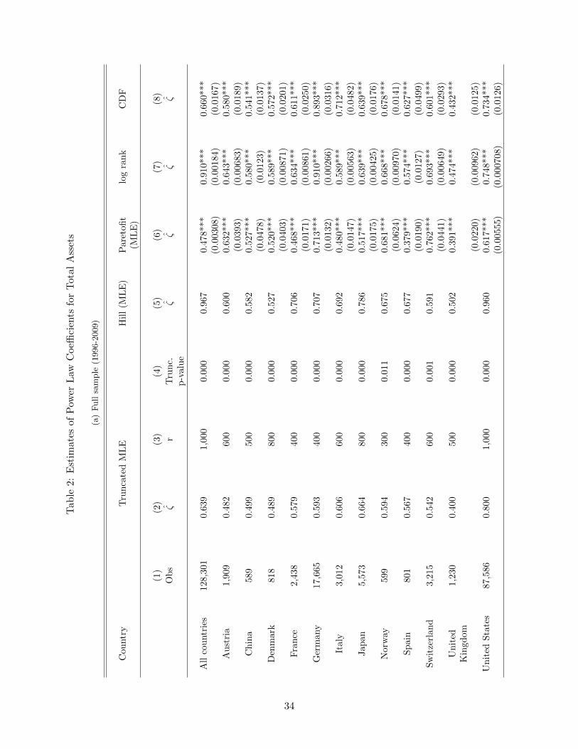
Tab

le2:

Est

imat

esof

Pow

erL

awC

oeffi

cien

tsfo

rT

otal

Ass

ets

(a)

Full

sam

ple

(1996-2

009)

Cou

ntr

yT

run

cate

dM

LE

Hill

(ML

E)

Pare

tofit

(ML

E)

log

ran

kC

DF

(1)

(2)

(3)

(4)

(5)

(6)

(7)

(8)

Ob

sζ

rT

runc.

p-v

alu

eζ

ζζ

ζ

All

countr

ies

128,

301

0.63

91,0

00

0.0

00

0.9

67

0.4

78***

0.9

10***

0.6

60***

(0.0

0308)

(0.0

0184)

(0.0

167)

Aust

ria

1,90

90.

482

600

0.0

00

0.6

00

0.6

32***

0.6

43***

0.5

80***

(0.0

393)

(0.0

0683)

(0.0

189)

Chin

a58

90.

499

500

0.0

00

0.5

82

0.5

27***

0.5

80***

0.5

41***

(0.0

478)

(0.0

123)

(0.0

137)

Den

mar

k81

80.

489

800

0.0

00

0.5

27

0.5

20***

0.5

89***

0.5

72***

(0.0

403)

(0.0

0871)

(0.0

201)

Fra

nce

2,43

80.

579

400

0.0

00

0.7

06

0.4

68***

0.6

34***

0.6

11***

(0.0

171)

(0.0

0861)

(0.0

250)

Ger

man

y17

,665

0.59

3400

0.0

00

0.7

07

0.7

13***

0.9

10***

0.8

93***

(0.0

132)

(0.0

0266)

(0.0

316)

Ital

y3,

012

0.60

6600

0.0

00

0.6

92

0.4

80***

0.5

89***

0.7

12***

(0.0

147)

(0.0

0563)

(0.0

482)

Jap

an5,

573

0.66

4800

0.0

00

0.7

86

0.5

17***

0.6

39***

0.6

39***

(0.0

175)

(0.0

0425)

(0.0

176)

Nor

way

599

0.59

4300

0.0

11

0.6

75

0.6

81***

0.6

68***

0.6

78***

(0.0

624)

(0.0

0970)

(0.0

141)

Sp

ain

801

0.56

7400

0.0

00

0.6

77

0.3

79***

0.5

74***

0.6

27***

(0.0

190)

(0.0

127)

(0.0

499)

Sw

itze

rlan

d3,

215

0.54

2600

0.0

01

0.5

91

0.7

62***

0.6

93***

0.6

01***

(0.0

441)

(0.0

0649)

(0.0

293)

Unit

edK

ingd

om1,

230

0.40

0500

0.0

00

0.5

02

0.3

91***

0.4

74***

0.4

32***

(0.0

220)

(0.0

0962)

(0.0

125)

Unit

edSta

tes

87,5

860.

800

1,0

00

0.0

00

0.9

60

0.6

17***

0.7

48***

0.7

34***

(0.0

0555)

(0.0

00708)

(0.0

126)

34

(b)

Cro

ssse

ctio

n(2

009)

Cou

ntr

yT

run

cate

dM

LE

Hill

(ML

E)

Pare

tofit

(ML

E)

log

ran

kC

DF

(1)

(2)

(3)

(4)

(5)

(6)

(7)

(8)

Ob

sζ

rT

runc.

p-v

alu

eζ

ζζ

ζ

All

countr

ies

10,5

410.

582

1,0

00

0.0

00

0.6

58

0.4

53***

0.9

00***

0.6

01***

(0.0

0308)

(0.0

0184)

(0.0

129)

Aust

ria

174

0.36

190

0.0

30.5

46

0.4

96***

0.5

62***

0.5

17***

(0.0

393)

(0.0

0683)

(0.0

172)

Chin

a86

0.32

180

0.0

40.4

93

0.4

29***

0.5

45***

0.4

81***

(0.0

478)

(0.0

123)

(0.0

142)

Den

mar

k80

0.38

065

0.2

40.5

02

0.4

08***

0.5

48***

0.5

15***

(0.0

403)

(0.0

0871)

(0.0

193)

Fra

nce

196

0.44

1126

0.0

50.5

77

0.3

58***

0.5

24***

0.4

84***

(0.0

171)

(0.0

0861)

(0.0

270)

Ger

man

y1,

204

0.74

6900

0.0

80.7

69

0.6

13***

0.8

24***

0.8

15***

(0.0

132)

(0.0

0266)

(0.0

260)

Ital

y44

70.

544

300

0.0

50.5

97

0.4

51***

0.5

98***

0.6

81***

(0.0

147)

(0.0

0563)

(0.0

418)

Jap

an47

60.

542

300

0.0

09

0.6

19

0.5

03***

0.6

31***

0.6

59***

(0.0

175)

(0.0

0425)

(0.0

281)

Nor

way

102

0.50

660

0.4

30.6

69

0.6

39***

0.6

70***

0.6

71***

(0.0

624)

(0.0

0970)

(0.0

226)

Sp

ain

114

0.37

950

0.1

80.7

96

0.3

52***

0.5

25***

0.5

80***

(0.0

190)

(0.0

127)

(0.0

515)

Sw

itze

rlan

d29

40.

373

50

0.3

30.5

35

0.7

18***

0.6

94***

0.5

99***

(0.0

441)

(0.0

0649)

(0.0

334)

Unit

edK

ingd

om10

50.

138

60

0.0

10.3

76

0.3

28***

0.3

82***

0.3

08***

(0.0

220)

(0.0

0962)

(0.0

0966)

Unit

edSta

tes

7,06

40.

624

400

0.0

09

691

0.6

17***

0.7

48***

0.7

38***

(0.0

0555)

(0.0

00708)

(0.0

128)

Note

s:T

his

table

pro

vid

eses

tim

ate

sfo

rth

ep

ower

law

shap

epara

met

erζ>

0of

the

cum

ula

tive

dis

trib

uti

on

funct

ion

of

banks’

tota

lass

ets

(in

1.0

00

USD

).r

isth

enum

ber

of

ord

erst

ati

stic

suse

dto

esti

mate

the

shap

epara

met

erof

the

trunca

ted

Pare

todis

trib

uti

on.

p-v

alu

eis

the

p-v

alu

eof

the

Pare

tote

st(H

0:

no

trunca

tion).

CD

Fes

tim

ate

sare

from

the

log

of

the

cum

ula

tive

dis

trib

uti

on

funct

ion,

as

des

crib

edin

Di

Gio

vanni

etal.

(2011).

Est

imate

sare

per

form

edex

cludin

gth

eb

ott

om

quart

ile

of

obse

rvati

ons,

usi

ng

robust

standard

erro

rsw

her

eapplica

ble

,and

clust

erin

gobse

rvati

ons

at

the

bank-l

evel

.In

the

log-r

ank

esti

mati

ons

over

the

full

sam

ple

(colu

mn

(7),

Table

2a),

tim

efixed

-eff

ects

are

incl

uded

.R

obust

standard

erro

rsare

giv

enin

bra

cket

s,and

*,

**,

***

indic

ate

ssi

gnifi

cance

at

the

10%

,5%

,and

1%

level

.

35

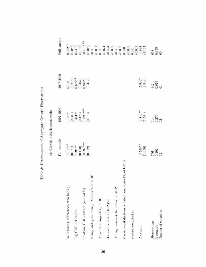
Table

3:D

eter

min

ants

ofA

ggre

gate

Gro

wth

Flu

ctu

atio

ns

(a)

Gro

wth

inlo

gdom

esti

ccr

edit

Fu

llsa

mp

le1997-2

006

2007-2

009

Fu

llsa

mple

BG

R(l

oan

s,d

iffer

ence

s,w

/ob

ank

j)0.2

15***

0.1

99**

0.1

26

0.2

02**

(0.0

77)

(0.0

81)

(0.2

15)

(0.0

87)

Log

GD

Pp

erca

pit

a0.2

98**

0.4

61**

0.6

69**

0.2

41*

(0.1

20)

(0.1

76)

(0.3

32)

(0.1

36)

Infl

atio

n,

GD

Pd

eflat

or(a

nnual

%)

-0.0

97***

-0.0

95***

0.8

40*

-0.1

01***

(0.0

12)

(0.0

13)

(0.4

72)

(0.0

12)

Mon

eyan

dqu

asi

mon

ey(M

2)as

%of

GD

P-0

.001

(0.0

01)

(Exp

orts

+im

por

ts)

/G

DP

0.0

31

(0.0

74)

Dom

esti

ccr

edit

/G

DP

(%)

-0.0

84

(0.0

89)

(For

eign

asse

ts+

liab

ilit

ies)

/G

DP

-0.0

01

(0.0

07)

Mar

ket

capit

aliz

atio

nof

list

edco

mp

anie

s(%

of

GD

P)

0.0

00

(0.0

00)

Z-s

core

,w

eigh

ted

av0.0

01

(0.0

01)

Con

stan

t-2

.540**

-3.8

43**

-5.8

86*

-1.9

34

(1.0

56)

(1.5

44)

(2.9

43)

(1.1

64)

Ob

serv

atio

ns

756

614

142

638

R-s

qu

ared

0.3

02

0.2

70

0.6

79

0.3

55

Num

ber

ofco

untr

ies

62

62

61

60

36

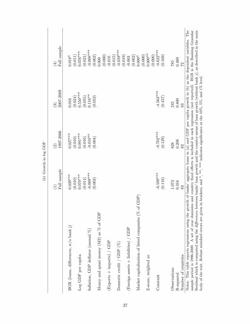
(b)

Gro

wth

inlo

gG

DP

(1)

(2)

(3)

(4)

Fu

llsa

mp

le1997-2

006

2007-2

009

Fu

llsa

mple

BG

R(l

oan

s,d

iffer

ence

s,w

/ob

ank

j)0.0

39***

0.0

27***

0.0

16

0.0

18*

(0.0

10)

(0.0

10)

(0.0

24)

(0.0

11)

Log

GD

Pp

erca

pit

a0.0

70***

0.0

91***

0.5

50***

0.0

76***

(0.0

14)

(0.0

16)

(0.0

55)

(0.0

21)

Infl

atio

n,

GD

Pd

eflat

or(a

nnual

%)

-0.0

09***

-0.0

10**

0.1

16**

-0.0

08***

(0.0

03)

(0.0

04)

(0.0

53)

(0.0

02)

Mon

eyan

dqu

asi

mon

ey(M

2)as

%of

GD

P0.0

00

(0.0

00)

(Exp

orts

+im

por

ts)

/G

DP

-0.0

10

(0.0

15)

Dom

esti

ccr

edit

/G

DP

(%)

-0.0

59***

(0.0

19)

(For

eign

asse

ts+

liab

ilit

ies)

/G

DP

-0.0

03

(0.0

02)

Mar

ket

capit

aliz

atio

nof

list

edco

mp

anie

s(%

of

GD

P)

0.0

00*

(0.0

00)

Z-s

core

,w

eigh

ted

av0.0

00**

(0.0

00)

Con

stan

t-0

.599***

-0.7

02***

-4.5

63***

-0.6

22***

(0.1

16)

(0.1

29)

(0.4

57)

(0.1

69)

Ob

serv

atio

ns

1,0

73

828

245

785

R-s

qu

ared

0.3

16

0.2

08

0.8

00

0.4

69

Num

ber

ofco

untr

ies

83

83

83

72

Note

s:T

his

table

rep

ort

sre

gre

ssio

ns

usi

ng

the

gro

wth

of

banks’

aggre

gate

loans

in(a

)and

GD

Pp

erca

pit

agro

wth

in(b

)as

the

dep

enden

tva

riable

s.T

he

sam

ple

per

iod

is1996-2

009.

Ase

tof

yea

rdum

mie

sand

countr

yfixed

effec

tsis

incl

uded

inea

chre

gre

ssio

n(n

ot

rep

ort

ed).

BG

Ris

the

Bankin

gG

ranula

rR

esid

ual

whic

his

com

pute

dusi

ng

the

diff

eren

ces

bet

wee

nbanks’

loan

gro

wth

and

the

countr

y-m

ean

of

loan

gro

wth

(wit

hout

bankj)

,as

des

crib

edin

the

main

body

of

the

text.

Robust

standard

erro

rsare

giv

enin

bra

cket

s,and

*,

**,

***

indic

ate

ssi

gnifi

cance

at

the

10%

,5%

,and

1%

level

.

37

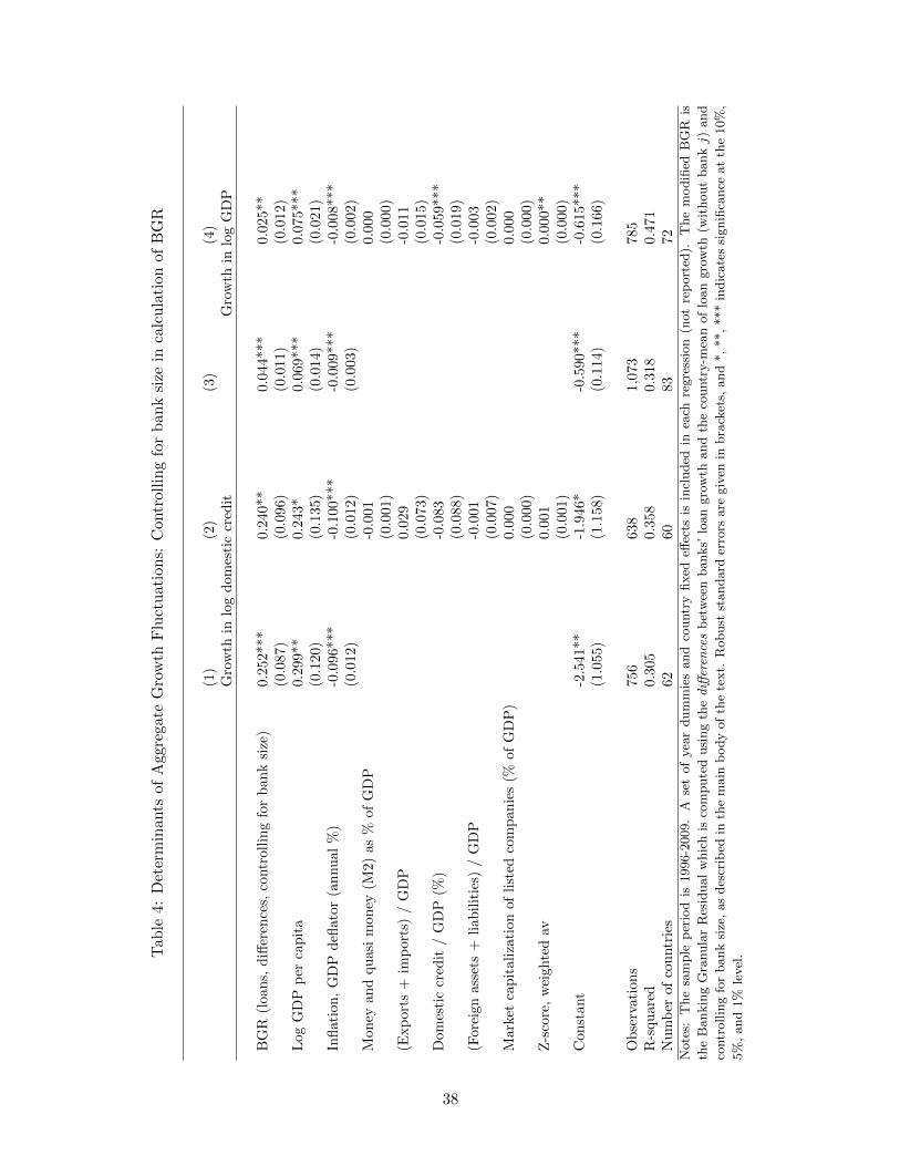
Table

4:

Det

erm

inan

tsof

Aggr

egat

eG

row

thF

luct

uat

ions:

Con

trol

lin

gfo

rb

ank

size

inca

lcu

lati

onof

BG

R

(1)

(2)

(3)

(4)

Gro

wth

inlo

gdom

esti

ccr

edit

Gro

wth

inlo

gG

DP

BG

R(l

oan

s,d

iffer

ence

s,co

ntr

ollin

gfo

rb

ank

size

)0.2

52***

0.2

40**

0.0

44***

0.0

25**

(0.0

87)

(0.0

96)

(0.0

11)

(0.0

12)

Log

GD

Pp

erca

pit

a0.2

99**

0.2

43*

0.0

69***

0.0

75***

(0.1

20)

(0.1

35)

(0.0

14)

(0.0

21)

Infl

atio

n,

GD

Pd

eflat

or(a

nnual

%)

-0.0

96***

-0.1

00***

-0.0

09***

-0.0

08***

(0.0

12)

(0.0

12)

(0.0

03)

(0.0

02)

Mon

eyan

dqu

asi

mon

ey(M

2)as

%of

GD

P-0

.001

0.0

00

(0.0

01)

(0.0

00)

(Exp

orts

+im

por

ts)

/G

DP

0.0

29

-0.0

11

(0.0

73)

(0.0

15)

Dom

esti

ccr

edit

/G

DP

(%)

-0.0

83

-0.0

59***

(0.0

88)

(0.0

19)

(For

eign

asse

ts+

liab

ilit

ies)

/G

DP

-0.0

01

-0.0

03

(0.0

07)

(0.0

02)

Mar

ket

capit

aliz

atio

nof

list

edco

mpanie

s(%

ofG

DP

)0.0

00

0.0

00

(0.0

00)

(0.0

00)

Z-s

core

,w

eigh

ted

av0.0

01

0.0

00**

(0.0

01)

(0.0

00)

Con

stan

t-2

.541**

-1.9

46*

-0.5

90***

-0.6

15***

(1.0

55)

(1.1

58)

(0.1

14)

(0.1

66)

Ob

serv

atio

ns

756

638

1,0

73

785

R-s

qu

ared

0.3

05

0.3

58

0.3

18

0.4

71

Num

ber

ofco

untr

ies

62

60

83

72

Note

s:T

he

sam

ple

per

iod

is1996-2

009.

Ase

tof

yea

rdum

mie

sand

countr

yfixed

effec

tsis

incl

uded

inea

chre

gre

ssio

n(n

ot

rep

ort

ed).

The

modifi

edB

GR

is

the

Bankin

gG

ranula

rR

esid

ual

whic

his

com

pute

dusi

ng

the

diff

eren

ces

bet

wee

nbanks’

loan

gro

wth

and

the

countr

y-m

ean

of

loan

gro

wth

(wit

hout

bankj)

and

contr

ollin

gfo

rbank

size

,as

des

crib

edin

the

main

body

of

the

text.

Robust

standard

erro

rsare

giv

enin

bra

cket

s,and

*,

**,

***

indic

ate

ssi

gnifi

cance

at

the

10%

,

5%

,and

1%

level

.

38

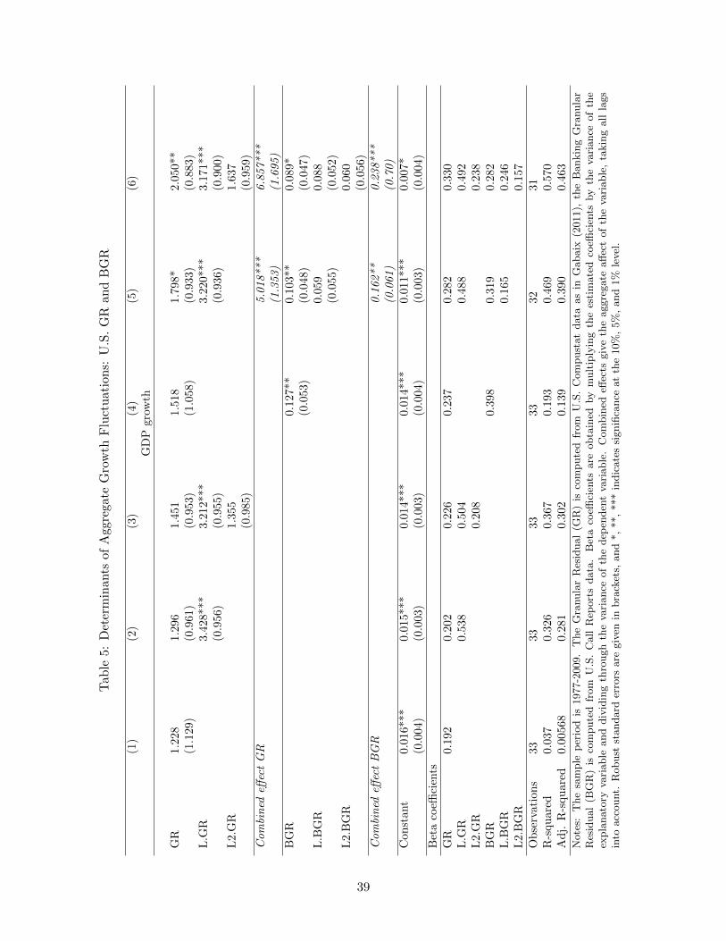
Table

5:

Det

erm

inan

tsof

Agg

rega

teG

row

thF

luct

uat

ions:

U.S

.G

Ran

dB

GR

(1)

(2)

(3)

(4)

(5)

(6)

GD

Pgro

wth

GR

1.22

81.

296

1.4

51

1.5

18

1.7

98*

2.0

50**

(1.1

29)

(0.9

61)

(0.9

53)

(1.0

58)

(0.9

33)

(0.8

83)

L.G

R3.

428*

**

3.2

12***

3.2

20***

3.1

71***

(0.9

56)

(0.9

55)

(0.9

36)

(0.9

00)

L2.

GR

1.3

55

1.6

37

(0.9

85)

(0.9

59)

Com

bin

edeff

ect

GR

5.0

18***

6.8

57***

(1.3

53)

(1.6

95)

BG

R0.1

27**

0.1

03**

0.0

89*

(0.0

53)

(0.0

48)

(0.0

47)

L.B

GR

0.0

59

0.0

88

(0.0

55)

(0.0

52)

L2.

BG

R0.0

60

(0.0

56)

Com

bin

edeff

ect

BG

R0.1

62**

0.2

38***

(0.0

61)

(0.7

0)

Con

stan

t0.

016*

**0.

015*

**

0.0

14***

0.0

14***

0.0

11***

0.0

07*

(0.0

04)

(0.0

03)

(0.0

03)

(0.0

04)

(0.0

03)

(0.0

04)

Bet

aco

effici

ents

GR

0.19

20.

202

0.2

26

0.2

37

0.2

82

0.3

30

L.G

R0.

538

0.5

04

0.4

88

0.4

92

L2.

GR

0.2

08

0.2

38

BG

R0.3

98

0.3

19

0.2

82

L.B

GR

0.1

65

0.2

46

L2.

BG

R0.1

57

Ob

serv

atio

ns

3333

33

33

32

31

R-s

qu

ared

0.03

70.

326

0.3

67

0.1

93

0.4

69

0.5

70

Adj.

R-s

qu

ared

0.00

568

0.28

10.3

02

0.1

39

0.3

90

0.4

63

Note

s:T

he

sam

ple

per

iod

is1977-2

009.

The

Gra

nula

rR

esid

ual

(GR

)is

com

pute

dfr

om

U.S

.C

om

pust

at

data

as

inG

abaix

(2011),

the

Bankin

gG

ranula

rR

esid

ual

(BG

R)

isco

mpute

dfr

om

U.S

.C

all

Rep

ort

sdata

.B

eta

coeffi

cien

tsare

obta

ined

by

mult

iply

ing

the

esti

mate

dco

effici

ents

by

the

vari

ance

of

the

expla

nato

ryva

riable

and

div

idin

gth

rough

the

vari

ance

of

the

dep

enden

tva

riable

.C

om

bin

edeff

ects

giv

eth

eaggre

gate

aff

ect

of

the

vari

able

,ta

kin

gall

lags

into

acc

ount.

Robust

standard

erro

rsare

giv

enin

bra

cket

s,and

*,

**,

***

indic

ate

ssi

gnifi

cance

at

the

10%

,5%

,and

1%

level

.

39

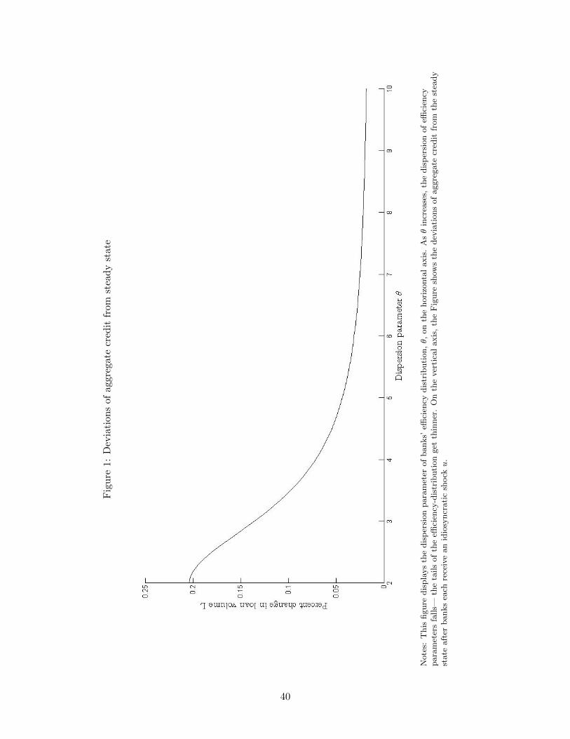
Fig

ure

1:D

evia

tion

sof

aggr

egat

ecr

edit

from

stea

dy

stat

e

Note

s:T

his

figure

dis

pla

ys

the

dis

per

sion

para

met

erof

banks’

effici

ency

dis

trib

uti

on,θ,

on

the

hori

zonta

laxis

.A

sθ

incr

ease

s,th

edis

per

sion

of

effici

ency

para

met

ers

falls—

the

tails

of

the

effici

ency

-dis

trib

uti

on

get

thin

ner

.O

nth

ever

tica

laxis

,th

eF

igure

show

sth

edev

iati

ons

of

aggre

gate

cred

itfr

om

the

stea

dy

state

aft

erbanks

each

rece

ive

an

idio

syncr

ati

csh

ocku

.

40

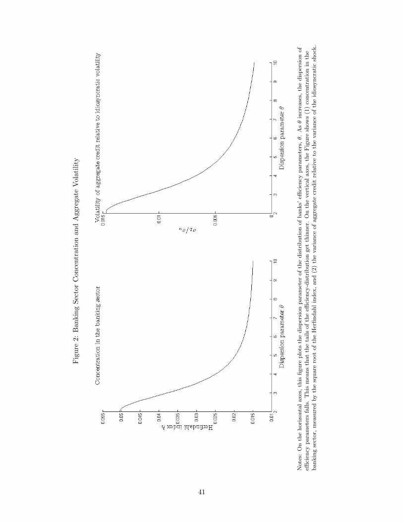
Fig

ure

2:B

ankin

gSec

tor

Con

centr

atio

nan

dA

ggre

gate

Vol

atilit

y

Note

s:O

nth

ehori

zonta

laxes

,th

isfigure

plo

tsth

edis

per

sion

para

met

erof

the

dis

trib

uti

on

of

banks’

effici

ency

para

met

ers,θ.

Asθ

incr

ease

s,th

edis

per

sion

of

effici

ency

para

met

ers

falls.

This

mea

ns

that

the

tails

of

the

effici

ency

-dis

trib

uti

on

get

thin

ner

.O

nth

ever

tica

laxes

,th

eF

igure

show

s(1

)co

nce

ntr

ati

on

inth

ebankin

gse

ctor,

mea

sure

dby

the

square

root

of

the

Her

findahl

index

,and

(2)

the

vari

ance

of

aggre

gate

cred

itre

lati

ve

toth

eva

riance

of

the

idio

syncr

ati

csh

ock

.

41

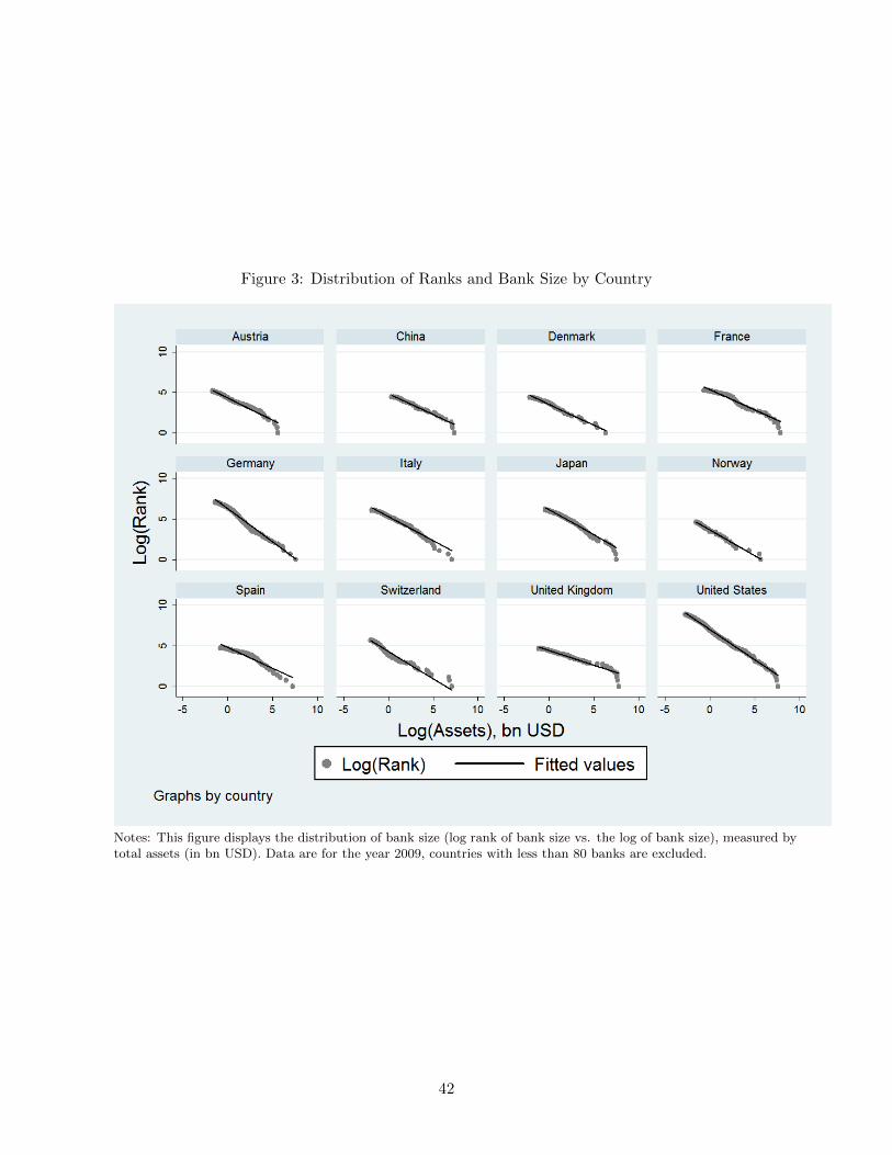
Figure 3: Distribution of Ranks and Bank Size by Country

Notes: This figure displays the distribution of bank size (log rank of bank size vs. the log of bank size), measured bytotal assets (in bn USD). Data are for the year 2009, countries with less than 80 banks are excluded.

42

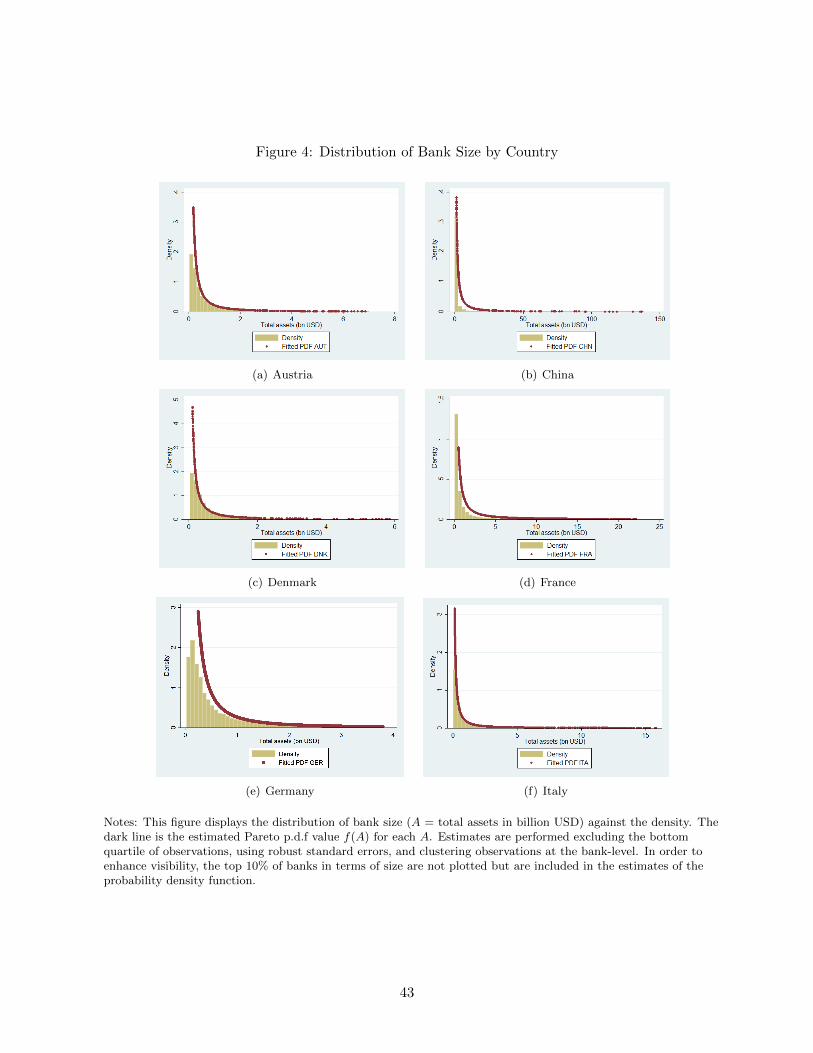
Figure 4: Distribution of Bank Size by Country

(a) Austria (b) China

(c) Denmark (d) France

(e) Germany (f) Italy

Notes: This figure displays the distribution of bank size (A = total assets in billion USD) against the density. Thedark line is the estimated Pareto p.d.f value f(A) for each A. Estimates are performed excluding the bottomquartile of observations, using robust standard errors, and clustering observations at the bank-level. In order toenhance visibility, the top 10% of banks in terms of size are not plotted but are included in the estimates of theprobability density function.

43

Figure 4 (continued)

(g) Japan (h) Norway

(i) Spain (j) Switzerland

(k) United Kingdom (l) United States

Notes: This figure displays the distribution of bank size (A = total assets in billion USD) against the density. Thedark line is the estimated Pareto p.d.f value f(A) for each A. Estimates are performed excluding the bottomquartile of observations, using robust standard errors, and clustering observations at the bank-level. In order toenhance visibility, the top 10% of banks in terms of size are not plotted but are included in the estimates of theprobability density function.

44

References

Aban, I., Meerschaert, M., and Panorska, A. (2006). Parameter estimation for the truncated pareto

distribution. Journal of the American Statistical Association, 101(473):270–277.

Adrian, T. and Brunnermeier, M. (2009). Covar. Federal Reserve Bank of New York Staff Report,

348(348).

Allen, J., Clark, R., and Houde, J. F. (2014). Search frictions and market power in negotiated price

markets. NBER Working Paper Series, (19883).

Allen, J., Clark, R., and Houde, J. F. (2015). Intermediaries and competition in markets with

search frictions. Manuscript, Bank of Canada.

Amiti, M. and Weinstein, D. (2013). How much do bank shocks affect investment? Federal Reserve

Bank of New York Staff Report, 604(604).

Anderson, S., De Palma, A., and Thisse, J. (1987). The CES is a discrete choice model? Economics

Letters, 24(2):139–140.

Andres, J. and Arce, O. (2012). Banking competition, housing prices and macroeconomic stability.

The Economic Journal, 122(565):1346–72.

Angeloni, I. and Faia, E. (2009). A tale of two policies: Prudential regulation and monetary policy

with fragile banks. Kiel Working Papers, 1569.

Ashcraft, A., McAndrews, J., and Skeie, D. (2011). Precautionary reserves and the interbank

market. Journal of Money, Credit, and Banking, 43:311–348.

Barbarasi, A.-L. and Albert, R. (1999). Emergence of scaling in random networks. Physica A:

Statistical Mechanics and its Applications, (3):509 – 512.

Barbarasi, A.-L., Albert, R., and Jeong, H. (1999). Mean-field theory for scale-free random net-

works. Physica A, 272:173 – 187.

Barth, J., Caprio, G., and Levine, R. (2001). The regulation and supervision of banks around the

world: A new database. World Bank Policy Research Working Paper, 2588.

45

Battacharya, K. (2003). How good is the bankscope database? BIS Working Papers.

Beck, T., Demirguc-Kunt, A., and Levine, R. (2000). A new database on financial development

and structure. World Bank Economic Review, 14:597–605.

Bharath, S., Dahiya, S., Saunders, A., and Srinivasan, A. (2011). Lending relationships and loan

contract terms. Review of Financial Studies, 24(4):1141–1203.

Blank, S., Buch, C., and Neugebauer, K. (2009). Shocks at large banks and banking sector distress:

The banking granular residual. Journal of Financial Stability, 5(4):353–373.

Bloom, N., Floetotto, M., Jaimovich, N., Saporta-Eksten, I., and Terry, S. (2012). Really uncertain

business cycles. NBER Working Paper No. 18245.

Broda, C. and Weinstein, D. E. (2006). Globalization and the gains from variety. The Quarterly

Journal of Economics, 121(2):541–585.

Buch, C. and Neugebauer, K. (2011). Bank-specific shocks and the real economy. Journal of

Banking & Finance, 35(8):2179–2187.

Carlson, M. and Mitchener, K. (2009). Branch banking as a device for discipline: Competition and

bank survivorship during the great depression. Journal of Political Economy, 117(2):165–210.

Carvalho, V. and Gabaix, X. (2013). The great diversification and its undoing. American Economic

Review, 103(5):1697–1727.

Corbae, D. and D’Erasmo, P. (2013). A quantitative model of banking industry dynamics. Working

Paper, University of Wisconsin.

Davies, R. and Tracey, B. (2014). Too big to be efficient? the impact of implicit subsidies on

estimates of scale economies for banks. Journal of Money, Credit and Banking, 46(s1):219–253.

De Blas, B. and Russ, K. (2013). All banks, great, small, and global. International Revew of

Economics and Finance, 26.

De Blas, B. and Russ, K. (2015). Understanding markups in the open economy. Americal Economic

Journal: Macroeconomics, 7(2).

46

DeAngelo, H., DeAngelo, L., and Stulz, R. (2006). Dividend policy and the earned/contributed

capital mix: a test of the life-cycle theory. Journal of Financial Economics, 81(2):227–254.

Denis, D. and Osobov, I. (2008). Why do firms pay dividends? international evidence on the

determinants of dividend policy. Journal of Financial Economics, 89(1):62–82.

Di Giovanni, J. and Levchenko, A. (2009). Trade openness and volatility. The Review of Economics

and Statistics, 91(3):558–585.

Di Giovanni, J. and Levchenko, A. (2012). Country size, international trade, and aggregate fluctu-

ations in granular economies. The Journal of Political Economy, 120(6):1083–1132.

Di Giovanni, J., Levchenko, A., and Mejean, I. (2014). Firms, destinations, and aggregate fluctua-

tions. Econometrica, 82(4):1303–40.

Di Giovanni, J., Levchenko, A., and Ranciere, R. (2011). Power laws in firm size and openness to

trade: Measurement and implications. Journal of International Economics, 85(1):42–52.

Dixit, A. and Stiglitz, J. (1977). Monopolistic competition and optimum product diversity. The

American Economic Review, pages 297–308.

Duprey, T. and Le, M. (2015). Bankscope dataset: getting started. Available at SSRN:

http://ssrn.com/abstract=2191449.

Freixas, X. and Rochet, J. (2008). Microeconomics of Banking. MIT Press Cambridge, MA and

London, 2 edition.

Gabaix, X. (2011). The granular origins of aggregate fluctuations. Econometrica, 79:733–772.

Gabaix, X. and Ibragimov, R. (2011). Rank-1/2: a simple way to improve the ols estimation of tail

exponents. Journal of Business & Economic Statistics, 29(1):24–39.

Gerali, A., Neri, S., Sessa, L., and Signoretti, F. (2010). Credit and Banking in a DSGE Model of

the Euro Area. Journal of Money, Credit and Banking, 42:107–141.

Ghironi, F. and Stebunovs, V. (2010). The domestic and international effects of interstate u.s.

banking. NBER Working Paper No. 16613.

47

Hale, G. (2012). Bank relationships, business cycles, and financial crises. Journal of International

Economics, 88(2):312 – 325.

Hale, G., Candelaria, C., Caballero, J., and Borisov, S. (2016). Bank linkages and international

trade. Federal Reserve Bank of San Francisco.

Hao, X. and Han, S. (2014). Operational risk transmission model of banks based on a scale-free

network. Hong Kong Institution of Engineers HKIE Transactions, 21(3):170–177.

Hill, B. (1975). A simple general approach to inference about the tail of a distribution. The Annals

of Statistics, 3(5):1163–1174.

James, M. and James, B. R. (1954). Biography of a bank: the story of Bank of America. Harper.

Jenkins, S. P. and Kerm, P. V. (2007). Paretofit: Stata module to fit a type 1 pareto distribution.

Available online at http://ideas.repec.org/c/boc/bocode/s456832.html.

Kalemli-Ozcan, S., Papaioannou, E., and Perri, F. (2012). Global banks and crisis transmission.

NBER Working Paper No. 18209.

Kashyap, A., Rajan, R., and Stein, J. (2002). Banks as liquidity providers: An explanation for the

coexistence of lending and deposit-taking. The Journal of Finance, 57(1):33–73.

Lustig, H. and Gandhi, P. (2015). Size Anomalies in U.S. Bank Returns. The Journal of Finance,

70(2):733–68.

Mandelman, F. (2010). Business cycles and monetary regimes in emerging economies: A role for a

monopolistic banking sector. Journal of International Economics, 81(1):122–138.

Meh, C. and Moran, K. (2010). The role of bank capital in the propagation of shocks. Journal of

Economic Dynamics and Control, 34(3):555–576.

Nickell, S. (1981). Biases in dynamic models with fixed effects. Econometrica, 49(6):1417 – 1426.

Pushkin, D. O. and Aref, H. (2004). Bank mergers as scale-free coagulation. Physica A: Statistical

Mechanics and its Applications, 336(3):571 – 584.

48

Sornette, D. (2006). Critical Phenomena in Natural Sciences: Chaos, Fractals, Selforganization

and Disorder: Concepts and Tools (Springer Series in Synergetics). Springer.

Tarashev, N., Borio, C., and Tsatsaronis, K. (2009). The systemic importance of financial institu-

tions. BIS Quarterly Review, 75:1–87.

Tarashev, N., Borio, C., and Tsatsaronis, K. (2010). Attributing systemic risk to individual insti-

tutions. BIS Working Paper, 308(308).

van Wincoop, E. (2013). International Contagion Through Leveraged Financial Institutions. Ame-

rican Economic Journal: Macroeconomics, 5(3):152–89.

Vives, X. (2016). Competition and Stability in Banking: The Role of Regulation and Competition

Policy. Princeton University Press.

Zhang, L. (2009). Bank capital regulation, the lending channel and business cycles. Deutsche

Bundesbank Discussion Paper Series 1: Economic Studies, 33(2009, 33).

49

A Maximization Problems

A.1 Firms

Firms maximize profits given by ΠF (i) = P (i)Y (i) − R(i)K(i) Demand for the firm’s good is

downward sloping in its price. Taking the derivative of the demand for any intermediate good with

respect to its price yields

∂Y (i)

∂P (i)= −µP (i)−µ−1PµY =

Y (i)

P (i).

Noting from the firm’s technology that K(i) = (1/α)Y (i), the first derivative of the firm profit

function with respect to price is given by

∂ΠF (i)

∂P (i)= Y (i) + P (i)

∂Y (i)

∂P (i)− R(i)

α

∂Y (i)

∂P (i)≡ 0 .

Then, substituting ∂Y (i)/∂P (i) into the derivative of the profit function yields the pricing equation

given in Eq.(7) of the main text.

A.2 Banks

The profit earned by bank j when serving firm i as given in the main text is

ΠB(i, j) = (1− δ)R(i, j)L(i, j)− 1

A(j)

[rdD(i, j) + reE(i, j)

].

We note that a fraction κ of the loan must be financed through equity, allowing the remainder to

be financed through deposits. Thus, the profit function can be rewritten as

ΠB(i, j) = (1− δ)R(i, j)L(i, j)− rd

A(j)[(1− κ) + (1 + τ)κ]L(i, j)

= (1− δ)R(i, j)L(i, j)− rd(1 + κτ)

A(j)L(i, j) .

We note that the external financing assumption and loan market clearing implies L(i, j) = K(i, j),

so that ∂L(i, j)/∂R(i, j) = −µL(i, j)/R(i, j). The first-order condition with respect to R(i, j) is

50

then

∂ΠB(i, j)

∂R(i, j)= (1− δ)

(L(i, j) +R(i, j)

∂L(i, j)

∂R(i, j)

)− rd(1 + κτ)

A(j)

∂L(i, j)

∂R(i, j)

= [(1− δ)− µ(1− δ)]L(i, j) +µrd(1 + κτ)

A(j)

L(i, j)

R(i, j)≡ 0 .

Cancelling L(i, j) in both terms and rearranging yields the unconstrained interest rate rule in the

main text.

B Applicability of the Levy Theorem

B.1 The restricted markup function is slowly varying

M(a) is slowly varying as long as, for any constant t greater than zero,

lima→∞

M(at)

M(a)= lim

a→∞

(1− v

[1−F (at)](at)µ−1Γ

) −1µ−1

(1− v

[1−F (a)](a)µ−1Γ

) −1µ−1

≡ 1 ,

which is true.

B.2 Bank size is power law distributed

Using Eq.(12) in the main text, the probability that an individual bank’s supply of credit is greater

than some positive constant l in steady state is given by

Pr(M(a)−µaµΦ > l

)= Pr

(M(a)−µaµ >

l

Φ

)= Pr

(M(a)−1a >

[l

Φ

] 1µ

)= l

θµΦ− θµψ(l) .

If the bank has a large enough efficiency parameter a such that it can charge the unrestricted

markup µµ−1 , then ψ(l) = M(a) = µ

µ−1 , a constant which is clearly a slowly varying function and

thus bank size follows a power law. Because lima→1

M(a) = ∞, then there must be some a < 1

above which all banks charge the (constant) unrestricted markup and the far-right tail is power-

law distributed up to the right truncation at a = 1. The dispersion parameter of the bank size

51

distribution, i.e. the exponent of loan volume l, is thus given by ζ = θµ . If ζ < 2, the bank size

distribution follows a fat-tailed power law.

We simulate the model to demonstrate that granular effects emerge in spite of the right trunca-

tion. In a first step, we compute the steady state values of our variables of interest (individual and

aggregate loans, Herfindahl index, volatility of loans), where u = 1. To that goal, we randomly draw

the intermediation indexes a for each of the J banks from a doubly truncated Pareto distribution.

Using these parameter draws, we can compute the aggregate price level P based on the unrestricted

loan rate. Using P , restricted loan rates and markups (restricted and unrestricted) are computed.

Based on these variables, we determine loan volumes for each firm, and we aggregate loans to total

credit for each repetition.

Second, a log-normally distributed shock u with mean one and a standard deviation of 0.01 is

assigned to each bank j, so that we can multiply the bank’s intermediation index, a · u. We then

compute the variables of interest for each bank including the shock to its intermediation index,

and then take the difference between aggregate loans and the Herfindahl index after and before the

shock. We repeat this procedure 1.000 times and average across repetitions.

We redo this exercise for the different values of the dispersion parameter θ of the intermediation

index a, such that µ− 1 < θ < 2µ.23

Regarding volatility, we compute the variance of aggregate loans across repetitions for each

value of theta.

We set the elasticity of substitution between goods, µ, equal to 3, close to the median estimate

in Broda and Weinstein (2006). We must discretize the number of banks and choose the number

J = 500, with 5.000 firms sending applications to a randomly chosen bank. In addition, we set

rd = 0.04 and a0 = 0.1, and, as scaling factors,α = 0.36, and Y = 10. The results of the simulation

are in Figures 1 and 2.

23This ensures that θµ< 2, the condition identified by Gabaix (2011) for granular effects to arise.

52

C Steady State

Firms:

Loan demand L(i, j) =1

α

µR(i,j)α(µ−1)

P

−µ YTechnology Y (i) = αL(i)

Optimal price P (i) =µ

α(µ− 1)R(i)

Banks:

Unrestricted loan rate R(i) =µ

µ− 1C(a)

Restricted loan rate R(i) =

[1− v

(1− F (a))Γaµ−1

] −1µ−1

C(a)

Aggregation and market clearing:

Aggregate loans L =

∫ J

0L(i, j)di

Aggregate price P =

(∫ 1

0P (i)1−µdi

) 11−µ

Aggregate production Y =

(∫ 1

0Y (i)

µ−1µ di

) µµ−1

53

D Bank concentration and aggregate credit volatility

This appendix illustrates that concentration in the banking sector is positively correlated with

aggregate credit volatility. In Table 6, we show that credit market concentration is positively cor-

related with the standard deviation of the aggregate credit supply once one controls for the average

risk of bank insolvency in each country, embodied in the average Z-score across the country’s banks.

Adding per capita GDP does not diminish the positive relationship between bank concentration and

variability in aggregate credit growth. Note that in this first glance at concentration and aggregate

credit variability, we have not yet accounted for differences in the lending growth of large versus

small banks. The relationship between banking sector concentration and aggregate volatility could

be driven by systemic factors and mitigated by monetary and regulatory policy differences across

countries. Thus, the question we ask now is whether concentration is correlated with aggregate

credit variability when we sum idiosyncratic changes in bank lending weighted by bank size (simi-

lar to our Herfindahl index but augmented by bank-level changes in credit growth). We then test

whether the second-order effect in our structural model – variability in aggregate credit and GDP

growth – also is associated with this size-weighted index of idiosyncratic lending shocks to link the

financial side of the economy with real outcomes.

54

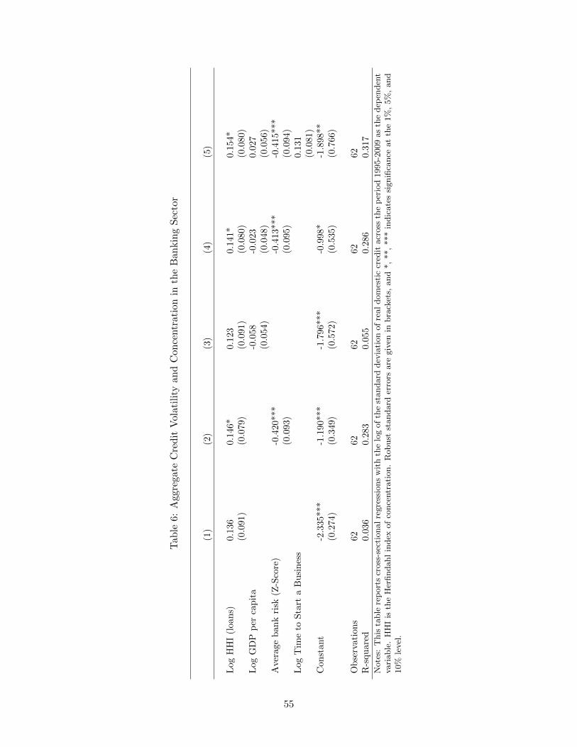
Table

6:

Agg

rega

teC

red

itV

olat

ilit

yan

dC

once

ntr

atio

nin

the

Ban

kin

gS

ecto

r

(1)

(2)

(3)

(4)

(5)

Log

HH

I(l

oan

s)0.

136

0.1

46*

0.1

23

0.1

41*

0.1

54*

(0.0

91)

(0.0

79)

(0.0

91)

(0.0

80)

(0.0

80)

Log

GD

Pp

erca

pit

a-0

.058

-0.0

23

0.0

27

(0.0

54)

(0.0

48)

(0.0

56)

Ave

rage

ban

kri

sk(Z

-Sco

re)

-0.4

20***

-0.4

13***

-0.4

15***

(0.0

93)

(0.0

95)

(0.0

94)

Log

Tim

eto

Sta

rta

Busi

nes

s0.1

31

(0.0

81)

Con

stan

t-2

.335

***

-1.1

90***

-1.7

96***

-0.9

98*

-1.8

98**

(0.2

74)

(0.3

49)

(0.5

72)

(0.5

35)

(0.7

66)

Ob

serv

atio

ns

6262

62

62

62

R-s

qu

ared

0.03

60.2

83

0.0

55

0.2

86

0.3

17

Note

s:T

his

table

rep

ort

scr

oss

-sec

tional

regre

ssio

ns

wit

hth

elo

gof

the

standard

dev

iati

on

of

real

dom

esti

ccr

edit

acr

oss

the

per

iod

1995-2

009

as

the

dep

enden

tva

riable

.H

HI

isth

eH

erfindahl

index

of

conce

ntr

ati

on.

Robust

standard

erro

rsare

giv

enin

bra

cket

s,and

*,

**,

***

indic

ate

ssi

gnifi

cance

at

the

1%

,5%

,and

10%

level

.

55