bode plots-lecture 1

8/8/2019 Bode Plots-Lecture 1

http://slidepdf.com/reader/full/bode-plots-lecture-1 1/30

Bode Plots

1Control lectures by Lubn Moin



From last class

Sketching the Root Locus for a given system

Determine the stability of the system basedon the R-L sketch




Today’s class

Sketching a bode diagram for a given system




Learning Outcomes

At the end of this lecture, students should be

able to: Sketch the bode diagram for a given system

Identify the system’s stability based on the

determined Gain Margin & Phase Margin




Frequency Response MethodFrequency Response Method

Frequency response analysis and design methodsFrequency response analysis and design methodsconsider response to sinusoids methods rather than stepsconsider response to sinusoids methods rather than steps

and ramps.and ramps.

Frequency response is readily determined experimentallyFrequency response is readily determined experimentally

in sinusoidal testingin sinusoidal testing..

Frequency response is readily obtained from the systemFrequency response is readily obtained from the system

transfer function (s =transfer function (s = j jωω) , where) , where ωω is the input frequency).is the input frequency).

Link between frequency and time domains is indirect.Link between frequency and time domains is indirect.

Design criteria help obtain good transient time response.Design criteria help obtain good transient time response.




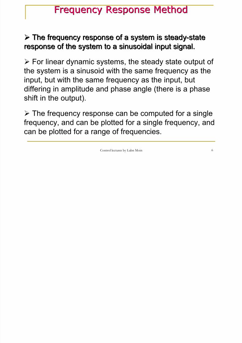
The frequency response of a system is steadyThe frequency response of a system is steady--statestate

response of the system to a sinusoidal input signal.response of the system to a sinusoidal input signal.

For linear dynamic systems, the steady state output of

the system is a sinusoid with the same frequency as the

input, but with the same frequency as the input, butdiffering in amplitude and phase angle (there is a phase

shift in the output).

The frequency response can be computed for a single

frequency, and can be plotted for a single frequency, and

can be plotted for a range of frequencies.

Frequency Response MethodFrequency Response Method




DecibelsDecibels

2 2 2

1 1 1

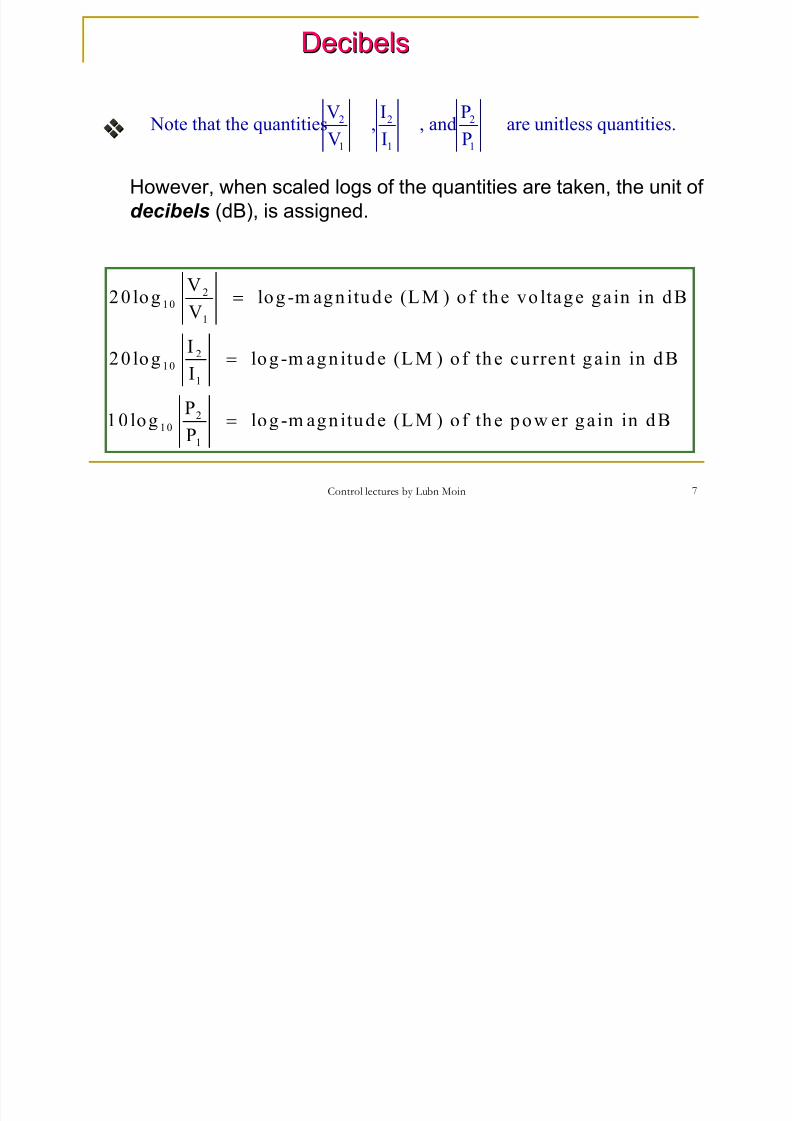
V I P Note that the quantities , , and are unitless quantities.

V I P

However, when scaled logs of the quantities are taken, the unit of decibels (dB), is assigned.

210

1

210

1

210

1

V20 log log -m agn itud e (LM ) o f the vo ltage gain in dB

V

I20 log log -m ag n itude (L M ) o f th e curren t gain in d BI

P10 log log -m agn itude (LM ) o f the p ow er gain in dB

P

=

=

=




There are two types of Bode plots:

The Bode straight-line approximation to the log-

magnitude (LM) plot, LM versus w (with w ona log scale)

The Bode straight-line approximation to the

phase plot, φ(w) versus w (with w on a logscale)




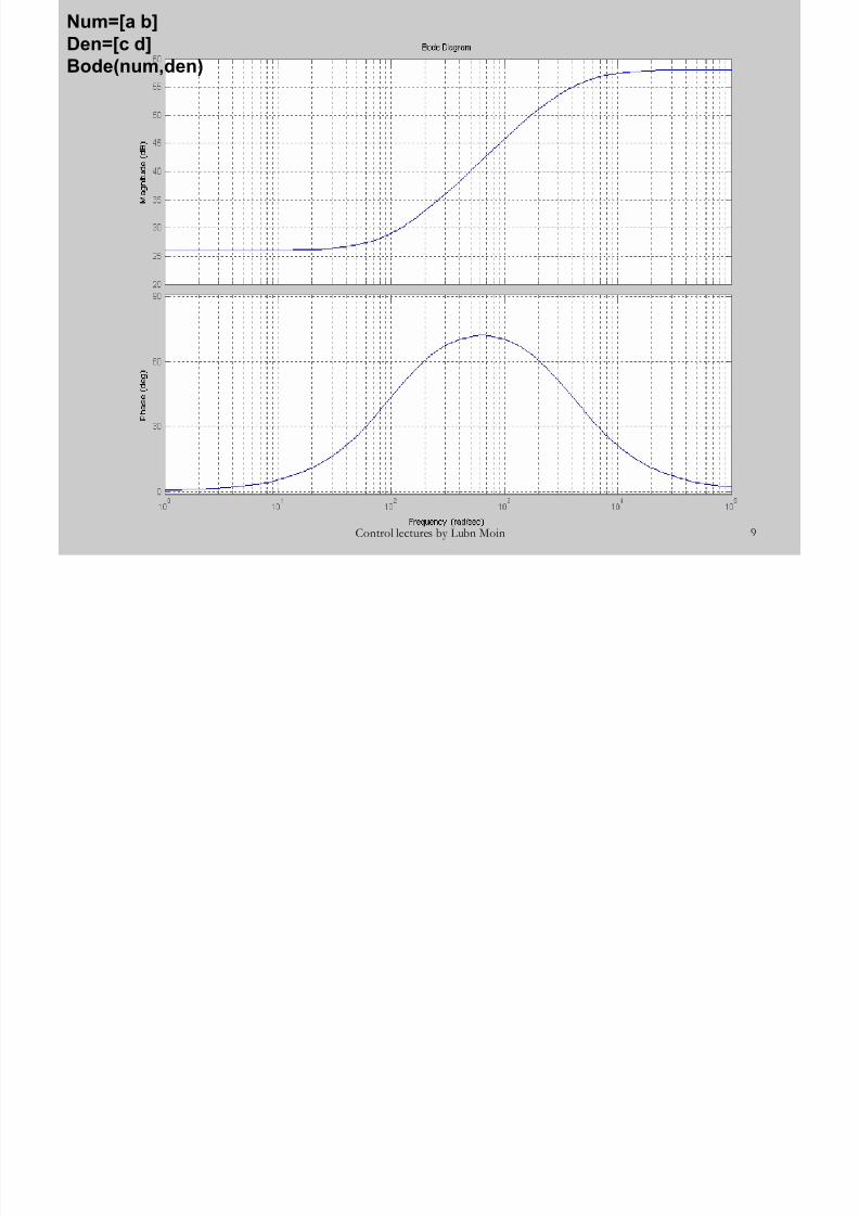
Num=[a b]

Den=[c d]

Bode(num,den)




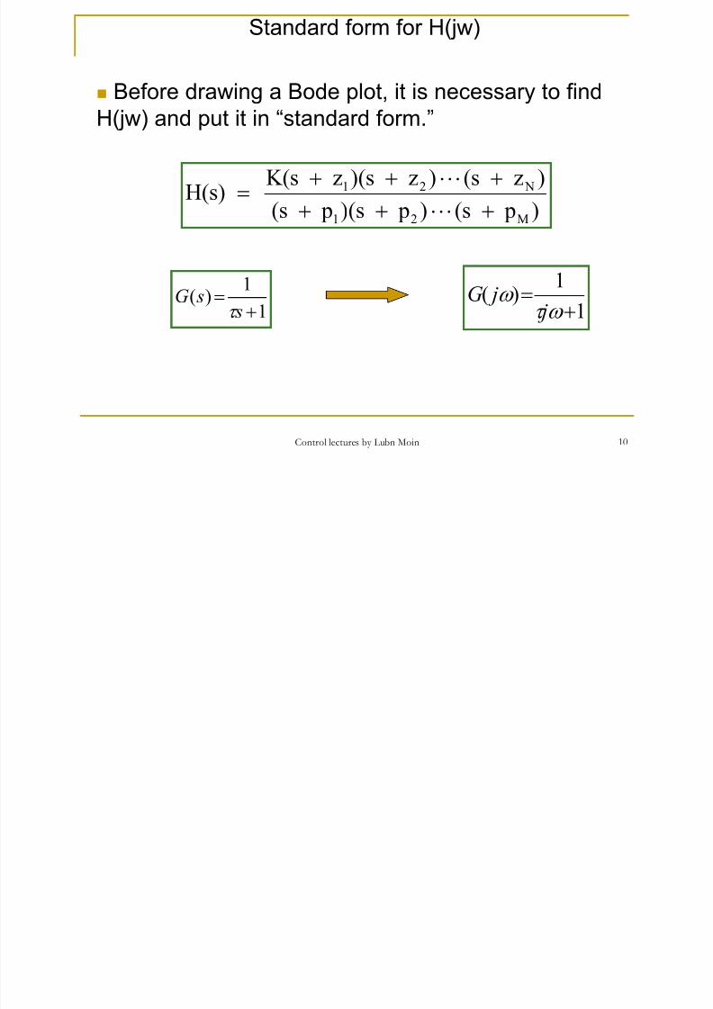
Standard form for H(jw)

Before drawing a Bode plot, it is necessary to find

H(jw) and put it in “standard form.”

1 2 N

1 2 M

K(s z )(s z ) (s z )H(s)

(s p )(s p ) (s p )

+ + ⋅ ⋅ ⋅ +=

+ + ⋅ ⋅ ⋅ +

1

1)(

+= s

sGτ 1

1)(

+=

ω τ ω

j jG




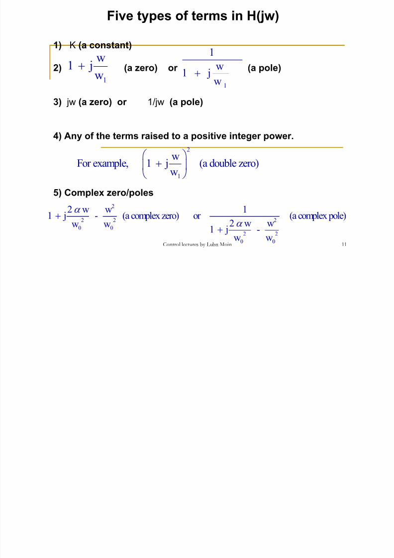
Five types of terms in H(jw)

1) K (a constant)

2) (a zero) or (a pole)

3) jw (a zero) or 1/jw (a pole)

4) Any of the terms raised to a positive integer power.

5) Complex zero/poles

1

w1 j

w+

2

2 2 2

0 02 2

0 0

2 w w 11 j - (a complex zero) or (a complex pole)

2 w ww w 1 j -w w

α

α

+

+

1

1

w1 j

w+

2

1

wFor example, 1 j (a double zero)

w

+




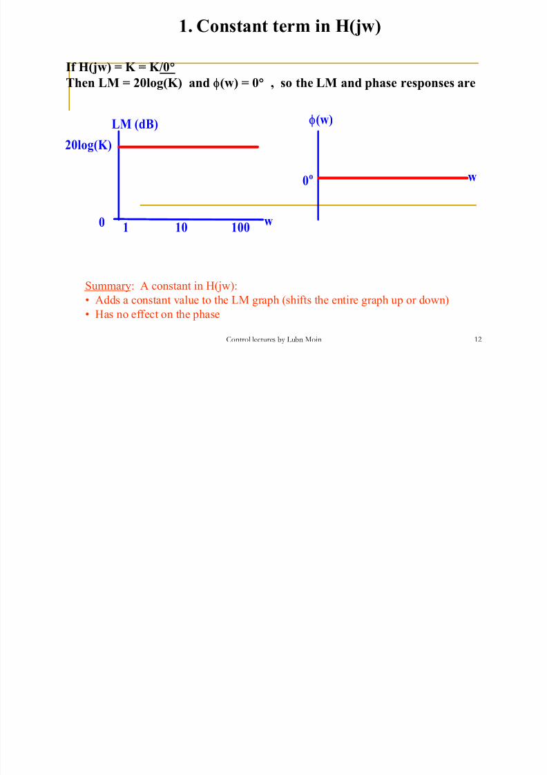
1. Constant term in H(jw)

If H(jw) = K = K/0°

Then LM = 20log(K) and φ(w) = 0° , so the LM and phase responses are

LM (dB)

w0

w

0

o

φ(w)

1

20log(K)

10 100

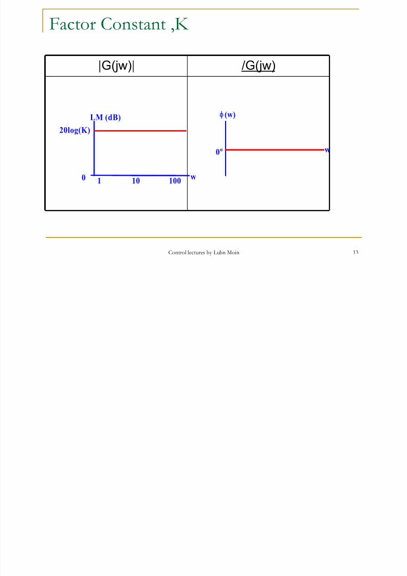
Summary: A constant in H(jw):

• Adds a constant value to the LM graph (shifts the entire graph up or down)

• Has no effect on the phase




Factor Constant ,K

|G(jw)| /G(jw)

LM (dB)

w0

w0o

φ (w)

1

20log(K)

10 100




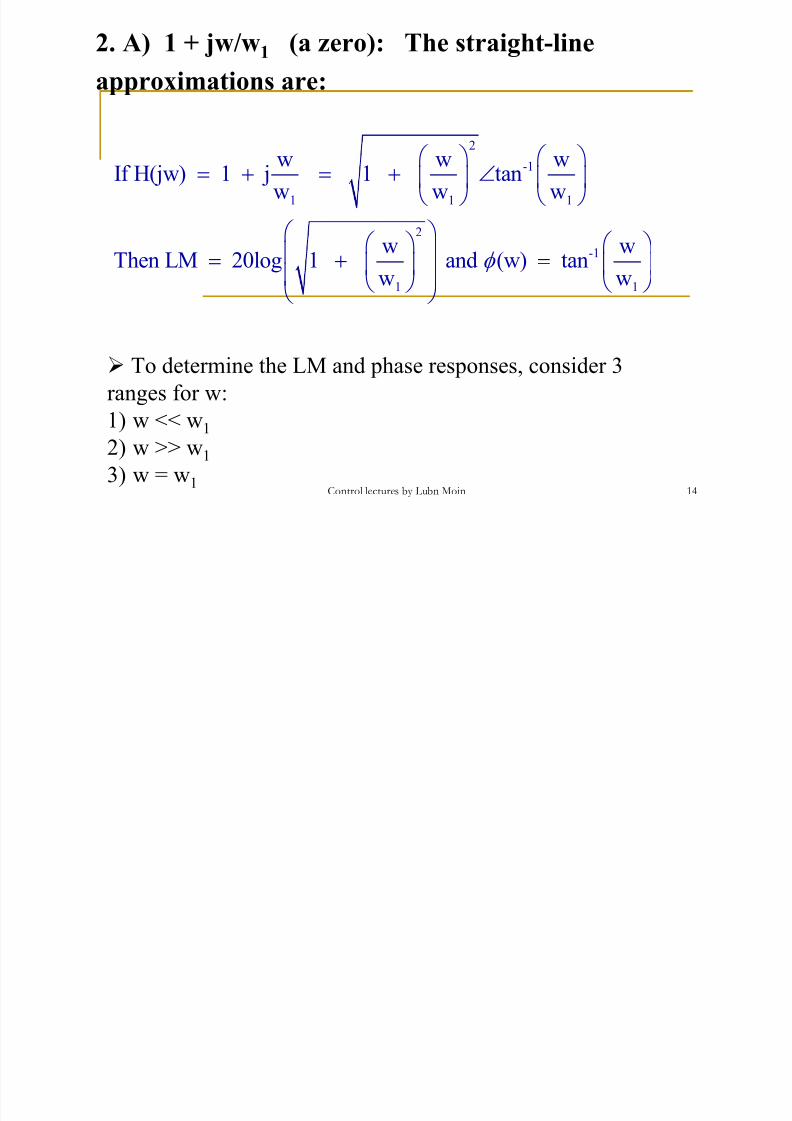
2. A) 1 + jw/w1 (a zero): The straight-line

approximations are:

2

-1

1 1 1

2

-1

1 1

w w w

If H(jw) 1 j 1 tanw w w

w w

Then LM 20log 1 and (w) tanw wφ

= + = + ∠

= + =

To determine the LM and phase responses, consider 3ranges for w:

1) w << w1

2) w >> w1

3) w = w114Control lectures by Lubn Moin



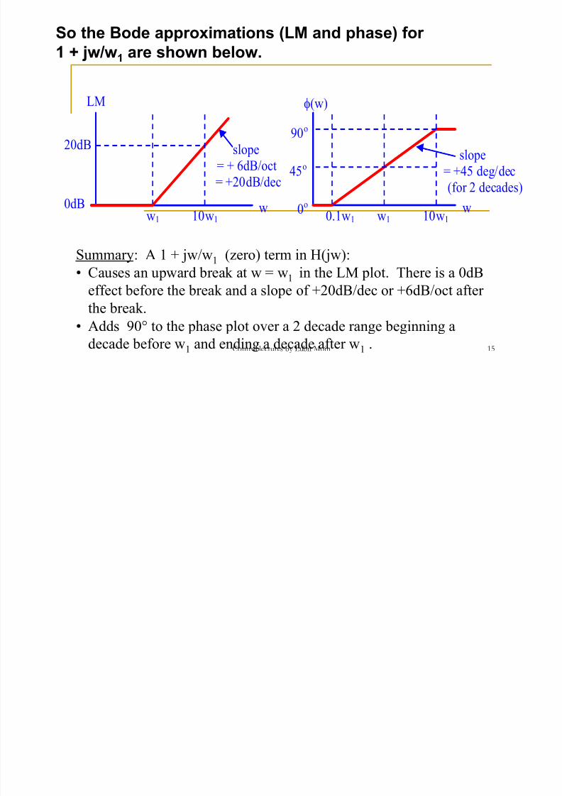
So the Bode approximations (LM and phase) for

1 + jw/w1 are shown below.

Summary: A 1 + jw/w1 (zero) term in H(jw):• Causes an upward break at w = w1 in the LM plot. There is a 0dB

effect before the break and a slope of +20dB/dec or +6dB/oct after

the break.

• Adds 90° to the phase plot over a 2 decade range beginning a

decade before w1 and ending a decade after w1 .

LM

w0dB

= +20dB/dec

w

90o

φ(w)

= + 6dB/oct

20dB

w1

slope

0o 10w1

45o

w1 10w1 0.1w1

= +45 deg/decslope

(for 2 decades)




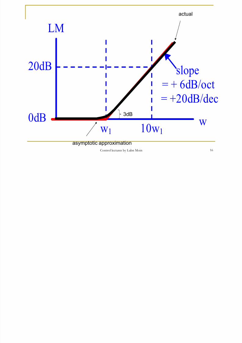
LM

w0dB

= +20dB/dec= + 6dB/oct

20dB

w1

slope

10w1

3dB

asymptotic approximation

actual


j



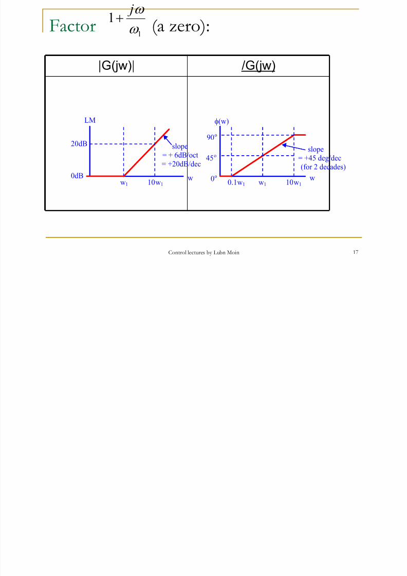
Factor (a zero):1

1ω

ω j+

|G(jw)| /G(jw)

LM

w0dB

= +20dB/dec

w

90o

φ(w)

= + 6dB/oct

20dB

w1

slope

0o

10w1

45o

w1 10w1 0.1w1

= +45 deg/decslope

(for 2 decades)




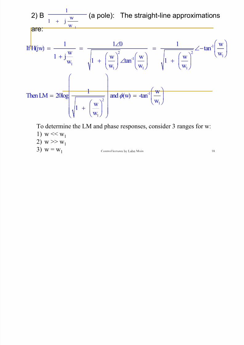
2) B (a pole): The straight-line approximations

are:

To determine the LM and phase responses, consider 3 ranges for w:

1) w << w1

2) w >> w1

3) w = w1

-1

2 2

1-1

11 1 1

-1

21

1

1 1 0 1 wIf H(jw) tan

ww1 j w w w1 tan 1w

w w w

1 wThen LM 20log and (w) -tan

ww

1 w

φ

∠= = = ∠−

+ + ∠ +

= =

+

1

1

w1 j

w

+




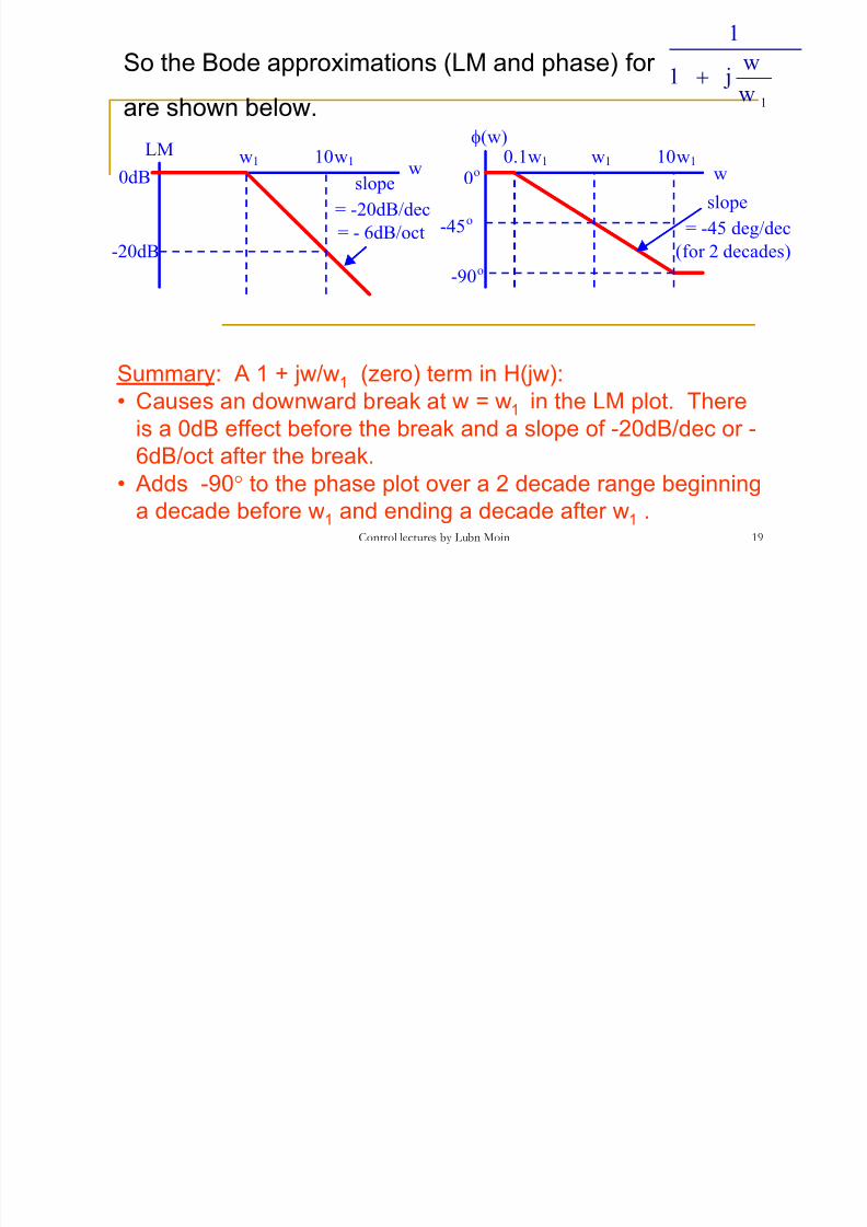
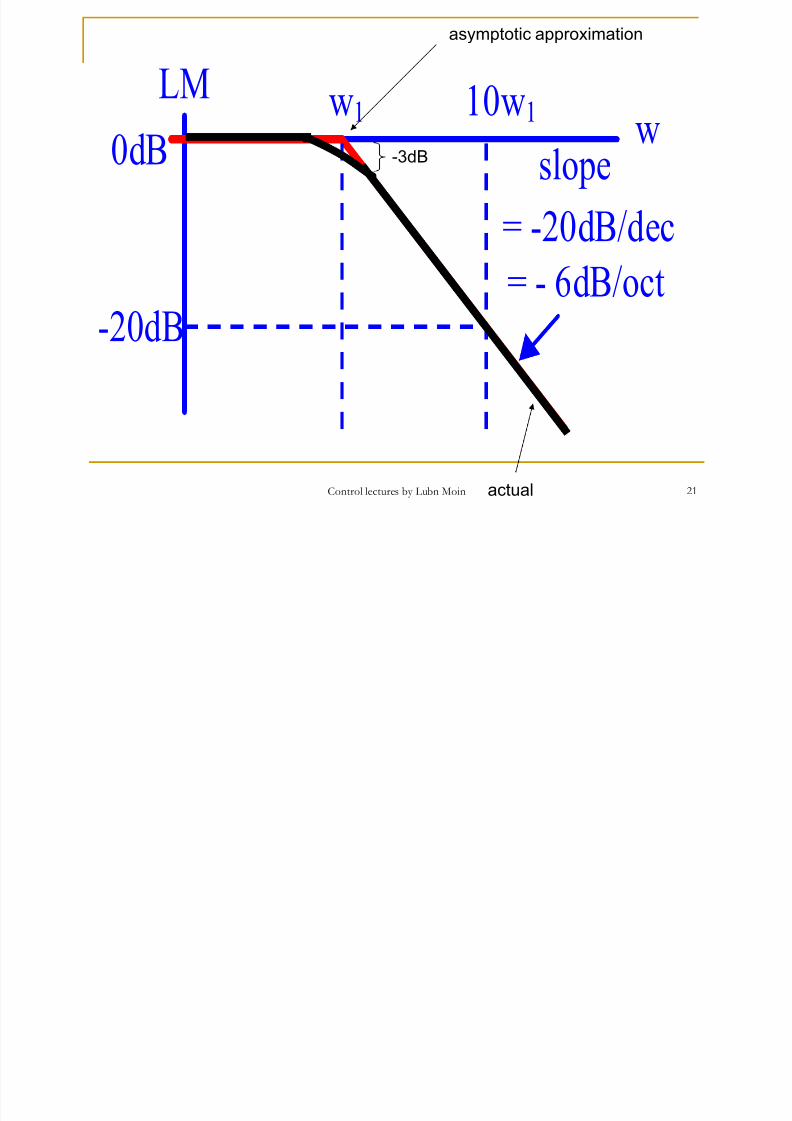
So the Bode approximations (LM and phase) for

are shown below. 1

1

w1 j

w

+

LMw

0dB

= -20dB/dec

w

-90o

φ(w)

= - 6dB/oct-20dB

w1

slope 0o 10w1

-45o

w1 10w1 0.1w1

= -45 deg/dec

slope

(for 2 decades)

Summary: A 1 + jw/w1 (zero) term in H(jw):

• Causes an downward break at w = w1 in the LM plot. Thereis a 0dB effect before the break and a slope of -20dB/dec or -

6dB/oct after the break.

• Adds -90°

to the phase plot over a 2 decade range beginninga decade before w1 and ending a decade after w1 .19Control lectures by Lubn Moin

1



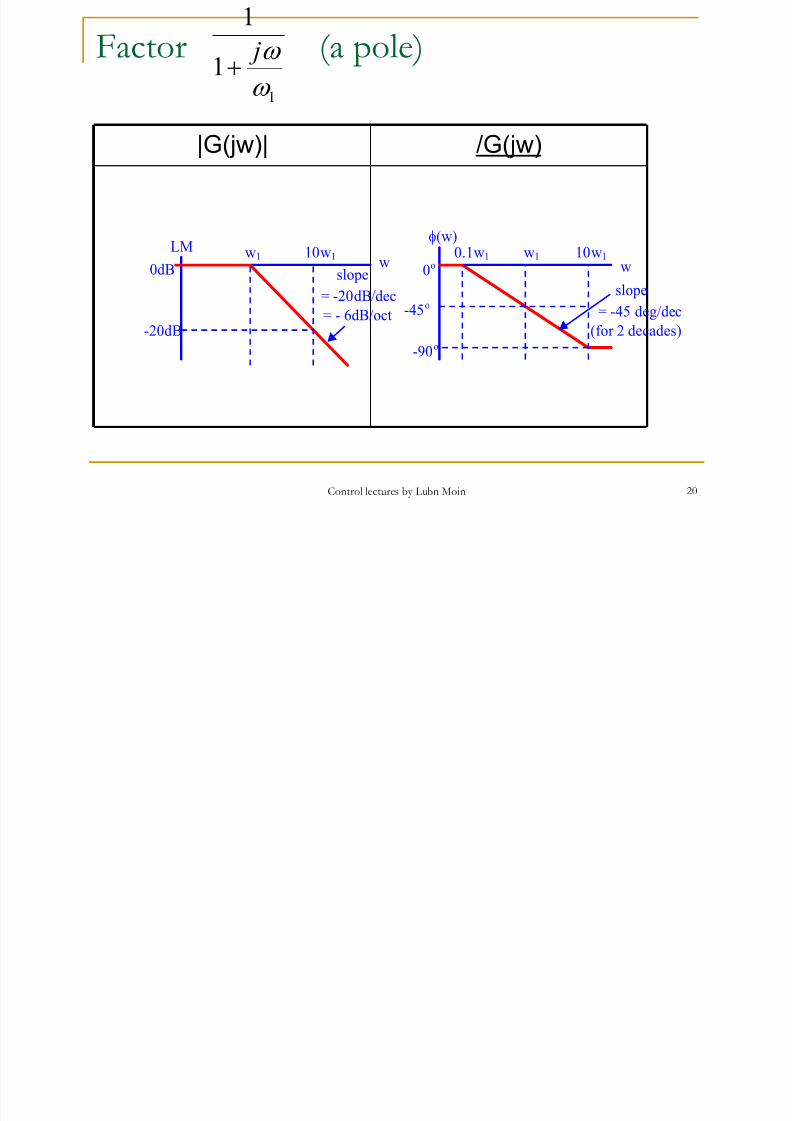
Factor (a pole)

1

1

1

ω

ω j+

|G(jw)| /G(jw)

LMw

0dB

= -20dB/dec

w

-90o

φ(w)

= - 6dB/oct-20dB

w1

slope 0o

10w1

-45o

w1 10w1 0.1w1

= -45 deg/dec

slope

(for 2 decades)




LM w0dB

= -20dB/dec

= - 6dB/oct-20dB

w1

slope

10w1 -3dB

asymptotic approximation

actual 21Control lectures by Lubn Moin



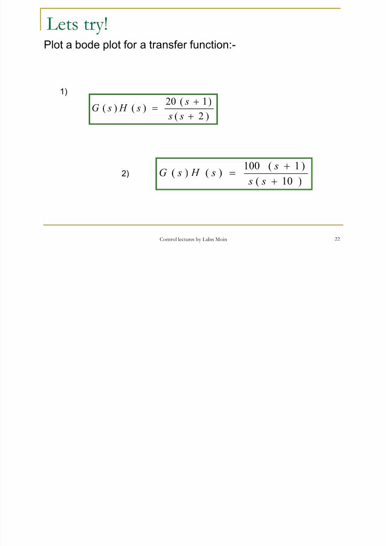
Lets try!

)2(

)1(20)()(

+

+=

s s

s s H sG

Plot a bode plot for a transfer function:-

)10(

)1(100

)()( +

+

= s s

s

s H sG

1)

2)




Reminder!!!

Don’t forget to bring:-

Ruler Pencil

Eraser

For Bode Plot Sketching…




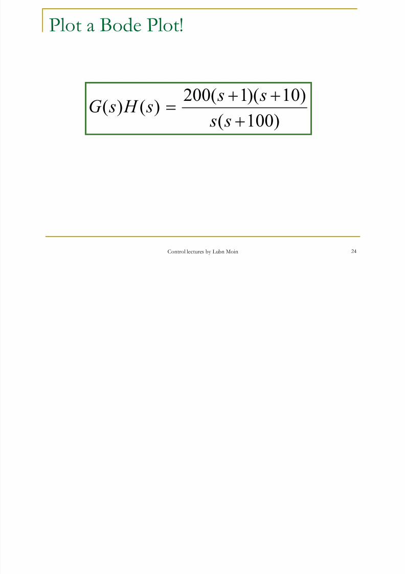
Plot a Bode Plot!

)100()10)(1(200)()(

+++=

s s s s s H sG




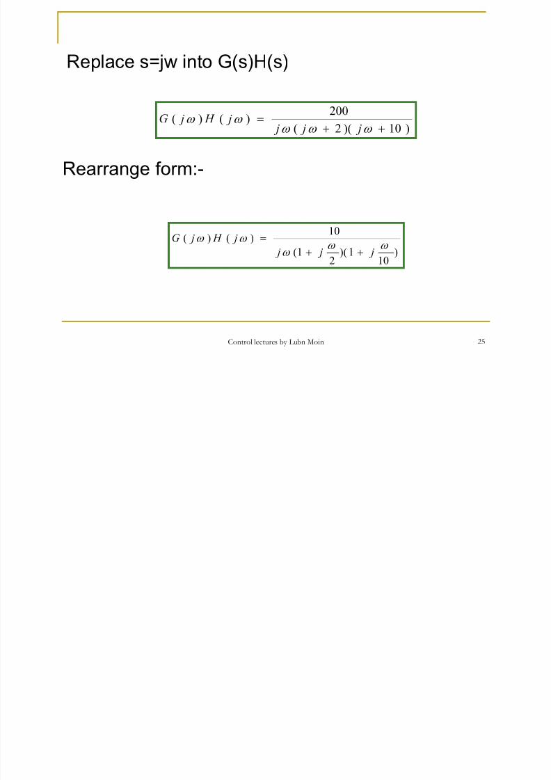
)10)(2(

200)()(

++

=ω ω ω

ω ω j j j

j H jG

Replace s=jw into G(s)H(s)

Rearrange form:-

)101)(21(

10)()(

ω ω ω

ω ω

j j j

j H jG

++

=




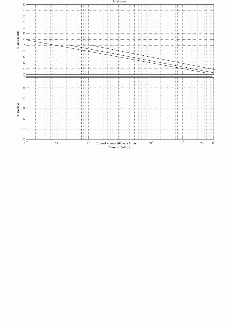
This transfer function has 4 forms:-

i. Factor Constant, K=10

ii. Factor

iii. Factor

iv. Factor

ω j

1

21

1

ω j+

101

1

ω

j+

Sketch for magnitude and phase!




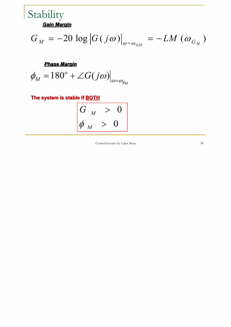
Stability

)()(log20M GM

GM LM jGG ω ω ω ω

−=−==

M jG

o

M φ ω ω ω φ =∠+=

)(180

Gain MarginGain Margin

Phase MarginPhase Margin

The system is stable if The system is stable if BOTHBOTH

0

0

>

>

M

M G

φ




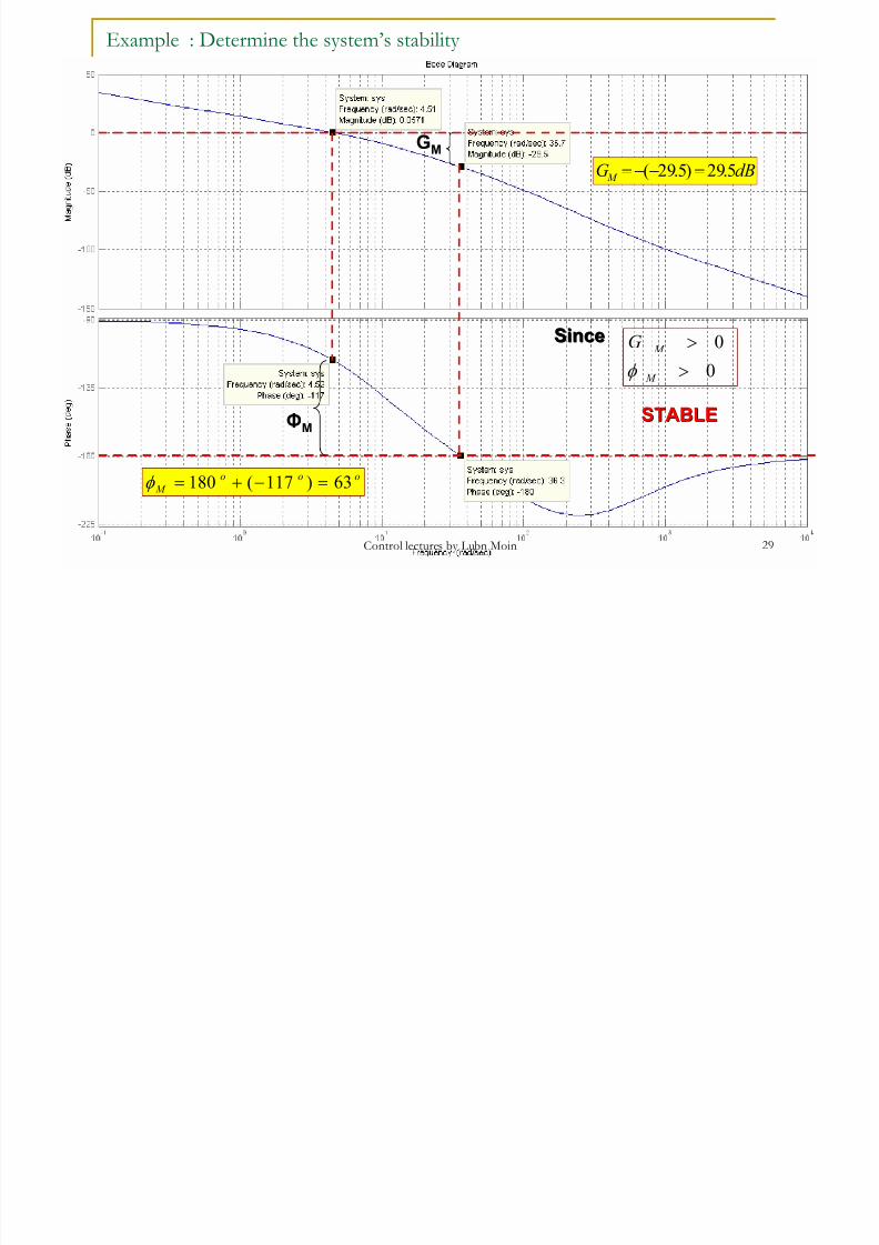
Example : Determine the system’s stability

GM

ΦM

dBGM 5.29)5.29( =−−=

ooo

M 63)117(180 =−+=φ

SinceSince

0

0

>

>

M

M G

φ

STABLESTABLE




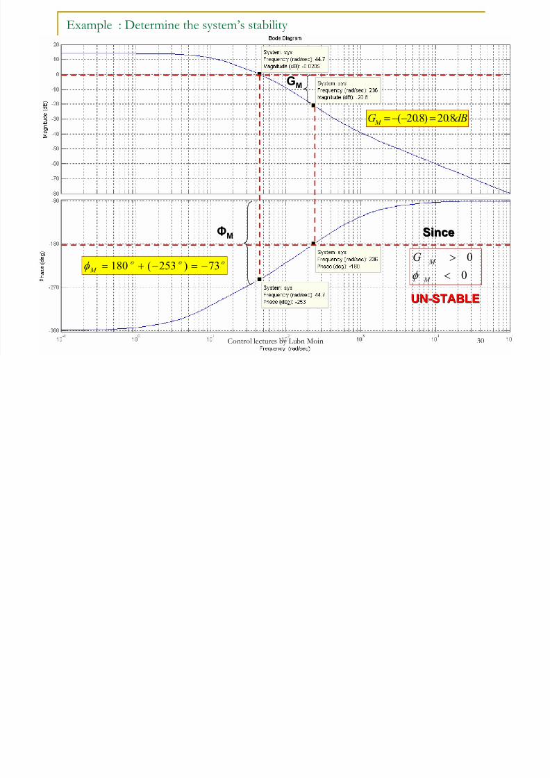
Example : Determine the system’s stability

GM

ΦM

dBGM 8.20)8.20( =−−=

ooo

M 73)253(180 −=−+=φ

SinceSince

0

0

<

>

M

M G

φ

UNUN--STABLESTABLE


bode plots-lecture 1

Documents