bucket-soil interaction for wheel...
TRANSCRIPT
Master's Thesis in Mechanical Engineering
Bucket-soil interaction for
wheel loaders - An application of the Discrete Element Method
Authors: Felix Henriksson, Joanna Minta
Supervisor LNU: Torbjörn Ekevid
Examiner LNU: Andreas Linderholt
Course code: 4MT31E
Semester: Spring 2016, 15 credits
Linnaeus University, Faculty of Technology


III
Abstract
Wheel loaders are fundamental construction equipment to assist handling of bulk
material e.g. gravel and stones. During digging operations, it withstands forces that
are both large and very complicated to predict. Moreover, it is very expensive to
develop prototypes of wheel loader for verification. Consequently, the Discrete
Element Method (DEM) was introduced for gravel modeling a couple of years ago to
enable prediction of these forces. The gravel model is connected with a Multibody
System (MBS) model of the wheel loader, in this thesis a Volvo L180G.
The co-simulation of these two systems is a very computer intensive operation and
hence, it is important to investigate which parameters that have the largest influence
on the simulation results. The aim of this thesis is to investigate the simulation
sensitivity with respect to co-simulation communication interval, collision detection
interval and gravel normal stiffness.
The simulation results are verified by comparison with measurement data from
previous tests performed by Volvo CE. The simulations are compared to investigate
the relevant parameters. The conclusion of this thesis is that DEM is a method that in
a very good way can predict the draft forces during digging operations.
Key words: Discrete element method, multibody system, wheel loader, soil-tool
interaction, co-simulation interval, gravel pile, collision detection interval, normal
stiffness.

IV
Acknowledgement
Foremost we would like to offer our sincerest gratitude to our supervisor Professor
Torbjörn Ekevid, Simulation Specialist at Volvo Construction Equipment. His help and
knowledge was invaluable. Thanks for patience, advices, necessary support and all
constructive comments.
Furthermore, we would like to thank Volvo Construction Equipment in Braås for
giving us the opportunity to perform our thesis in cooperation with them. We are
really grateful to Lennarth Zander, Manager Analysis, for providing us workspace and
equipment.
We would also like to thank Andreas Linderholt, Head of Mechanical Engineering
Department at Linnaeus University and Åsa Bolmsvik, Senior Lecturer at Linnaeus
University.
For unconditional support during this time we offer our heartfelt thanks to our family and
friends.
____________________ ____________________
Felix Henriksson Joanna Minta
Växjö 25th of May 2016
V
Table of contents
1. INTRODUCTION ......................................................................................................... 1
1.1 BACKGROUND ................................................................................................................................... 1 1.2 AIM AND PURPOSE ............................................................................................................................. 3 1.3 LIMITATIONS ..................................................................................................................................... 3 1.4 RELIABILITY, VALIDITY AND OBJECTIVITY ........................................................................................ 3
2. THEORY AND LITERATURE REVIEW ................................................................. 5
2.1 GEOLOGICAL MATERIALS.................................................................................................................. 5 Soil Mechanics .......................................................................................................................... 5
2.2 DISCRETE ELEMENT METHOD ........................................................................................................... 8 Law of Motion ........................................................................................................................... 9 The Force-Displacement Law ................................................................................................. 10 Determination of Forces Acting on the Bucket ....................................................................... 14 DEM Implementation .............................................................................................................. 16 DEM Software ........................................................................................................................ 18
2.3 MULTIBODY SYSTEMS ..................................................................................................................... 18 Simulation of Multibody Systems ............................................................................................ 18
2.4 SIMULATION OF DYNAMIC SYSTEMS ............................................................................................... 19
3. METHOD ..................................................................................................................... 20
3.1 TOTAL SIMULATION MODEL ............................................................................................................ 20 Discrete Element Method ....................................................................................................... 20 Multibody System Simulation.................................................................................................. 21 Simulink .................................................................................................................................. 22
3.2 THE ASSEMBLED MODEL ................................................................................................................. 22 3.3 COLLECTION OF DATA ..................................................................................................................... 24
Simulated Data ....................................................................................................................... 24 Measured Data ....................................................................................................................... 26
4. RESULTS AND ANALYSIS ...................................................................................... 28
4.1 SIMULATION SETUPS ....................................................................................................................... 28 4.2 BASELINE SIMULATION COMPARED TO MEASUREMENT .................................................................. 28 4.3 SIMULATIONS COMPARED TO SIMULATIONS.................................................................................... 30
Co-Simulation Interval ........................................................................................................... 31 Collision Detection Interval.................................................................................................... 37 Normal Stiffness ...................................................................................................................... 41
5. DISCUSSION .............................................................................................................. 47
6. CONCLUSIONS ......................................................................................................... 48
REFERENCES ................................................................................................................. 49
APPENDIXES .................................................................................................................. 51

1
Felix Henriksson, Joanna Minta
1. Introduction
Wheel loaders and excavators are machines that are used to perform digging
operations to assist movement of materials like gravel, sand and stone in all
types of suitable applications [1]. Consequently, since a lot of different
materials can be handled under different circumstances, the loads acting on
the bucket are difficult to predict. Due to these uncertainties the design of a
wheel loader or excavator bucket is very complicated [2]. In addition, the
customers of this equipment expect a product with high reliability [3].
These influences could lead to a bucket with excessive dimensions, which of
course provides a reliable product but with one major drawback i.e. increase
of weight [2]. The increased weight will cause higher energy consumption
and less productivity, and as in any other technology area the aim is to
minimize the fuel consumption and simultaneously increase the performance
[3]. To reach these contradictory objectives, the development has to be done
in a correct way. Since prototype development of machines like wheel
loaders and excavators are very expensive, simulations are used at an early
design stage for validation.
The wheel loaders and excavators can be simulated using Multibody
Simulation (MBS), which is a conventional method in vehicle development.
However, it is not feasible to simulate the interaction between gravel and
bucket with this method because MBS is not suitable for applications
including collision between a large number (~100000) of particles.
Accordingly, another solution is applied for this application, the Discrete
Element Method (DEM). The research in this field is ongoing and it is
applied in small scale for modeling and simulation of soil combined with
MBS models. The advantage with DEM is that the soil can be modeled as
single elements where it is possible to set properties depending on the soil
type and its behavior.
1.1 Background
Volvo Construction Equipment (Volvo CE) is one of the world’s leading
manufacturers of construction equipment vehicles. They are supplying the
construction industry with a wide range of vehicles, for instance wheel
loaders, excavators and articulated haulers. For the last two decades Volvo
CE has applied Multibody simulations (MBS) to model vehicles and its
subsystems. This method is well implemented using the software Adams [4]
where virtual tests of a complete vehicle can be performed. MBS was first
used to virtually analyze the driving characteristics of a vehicle. However,
during the last five years the use of MBS has been expanded to also include
load acquisition i.e. generating design loads. This allows validation of the
design at an early stage. Since the virtual tests have proven very resourceful,

2
Felix Henriksson, Joanna Minta
the target is to increase the range of vehicles, components and driving cases
that can be modeled and analyzed with simulation.
As a result of this intention, to expand the usage of simulations, Volvo CE
acknowledged a new potential area to apply simulations i.e. the digging
operations performed by wheel loaders and excavators. Since it is difficult to
predict the loads during these operations, the design gets complicated.
Subsequently Volvo CE initiated research of this topic approximately five
years ago. It turned out that the most convenient way to model the gravel is
by use of the Discrete Element Method (DEM) [5], a method that other
companies studied as well [6]. DEM is a numerical method that is used to
model, simulate and predict the behavior of, for instance, granular materials
[7]. Except for this topic, DEM is also applicable in other fields such as food
industry and chemical science for pharmaceutical development [8].
However, this thesis will treat the prediction of the dynamic behavior of
gravel material and its interaction with the bucket.
Volvo CE first applied DEM to simulate the filling process of an excavator
bucket with the software Pasimodo [9]. Since the first application was
successful, Volvo CE expanded their research and application of DEM to
also cover the impact load from gravel on the bucket, and the present
software used by Volvo CE is GRAPE from Fraunhofer ITWM [10].
Although DEM has many advantages it also has drawbacks, and one of the
most challenging tasks is to capture the real behavior of the gravel with
retained result accuracy without demanding unlimited computational
resources. For instance, to simplify the computations, single grains will be
modeled as spherical elements, which is not the case in reality.
Consequently, the impact from the irregular particle shape has to be
compensated in the model. This could be done by adjustment of gravel
parameters such as rolling resistance, normal stiffness and friction
coefficient [3]. The influence of normal stiffness will be investigated in this
thesis.
A further challenge for Volvo CE, since the wheel loaders and excavators
are modeled in Adams, is to maintain the connection between the DEM
software with Adams in an effective way. Since other systems i.e. the
powertrain and hydraulics are modeled in Simulink [11] this software will
serve as bridge. The whole setup is very computationally intensive and thus
the computation needs to be optimized to achieve the most convenient
tradeoff between computational time and result accuracy. The essential
parameter for controlling this tradeoff is the co-simulation communication
interval between the software, i.e. how frequent the different software
updates against each other. This aspect will among other things be
investigated in this thesis.
Thus, the intended outcome of this thesis is to improve the simulation
procedure of the gravel-bucket interaction. This will allow verified
3
Felix Henriksson, Joanna Minta
calculations at an early design stage and more accurate optimization of the
bucket. If it is possible to reduce the sheet metal thickness and other design
parameters of the bucket, the bucket weight will consequently decrease.
Subsequently this will lead to reduced energy consumption and improved
performance.
1.2 Aim and Purpose
The aim of this thesis is to investigate the sensitivity to the co-simulation
communication interval between Adams, Simulink and GRAPE regarding
performance and stability. Furthermore, the aim is to investigate the impact
of the gravel material property, normal stiffness.
The purpose of this thesis is to contribute to at an early design stage allow
verified designs for wheel loader and excavator buckets. Additionally, the
purpose is to determine the loads acting on the bucket when performing
digging operations. This enables the opportunities to optimize the bucket
regarding parameters as dimensions and weight.
1.3 Limitations
This thesis is limited to simulations of existing models in Adams of the
wheel loader and the DEM software GRAPE of the gravel that are connected
with Simulink. Hence, the results of this thesis will be extracted from
simulations of the existing models. Thus, no modeling will be done from
scratch, only slight modifications on the existing models if needed will be
carried out.
The wheel loader bucket is limited to one type, a re-handling bucket. That is
a bucket intended for gravel handling without teeth.
The investigated aspects are limited to the sensitivity of the co-simulation
communication interval and the gravel grain normal stiffness. Another
limitation regarding the DEM model is that the single grains will be
modeled as spherical particles with three degrees of freedom. This limitation
is done to use the computational resource in the most effective way.
1.4 Reliability, validity and objectivity
To achieve a reliable and valid study, it is required that the correct and
relevant measuring equipment are used properly. The main measuring
equipment in this study is computer software i.e. GRAPE, Adams and
Simulink. All of these are required to fulfill the aim and purpose of the
thesis.

4
Felix Henriksson, Joanna Minta
The reliability and validity in this thesis will be upheld through comparison
with available tests data. The simulations will also be done of more than one
person under supervision of experienced personnel and at Volvo CE.
Even though this thesis is focused on a bucket from a Volvo CE wheel
loader the objectivity is withheld since all methods are generally described
and subsequently applicable for any soil-tool interaction.

5
Felix Henriksson, Joanna Minta
2. Theory and Literature Review
In the following chapter, theories and literature that are relevant to the thesis
are described.
2.1 Geological Materials
Geological materials are natural resources that could be found in the crust of
the earth i.e. rocks, minerals, water and soil [12]. These are fundamental for
some parts of the modern society i.e. agriculture, industry and construction
[13]. They are a part of the field Engineering Geology and some of the
specific subjects in this field are geotechnical processes, foundation
engineering and soil mechanics. Soil mechanics is an important aspect in
this thesis and will be presented in more detail.
Soil Mechanics
Soils are one of the most important natural resources on earth and play an
important role in building construction as foundation and support [3, 13].
Furthermore, the properties of the soil influence the design of equipment
used for soil-tool interaction. Soil can roughly be categorized into three
different classifications i.e. cohesionless, cohesive and cemented soil [14].
The difference between them is the bond between single particles. Of these
three categories, cemented soil has the strongest bonds and cohesionless the
weakest. Cemented soils are compound with a bonding agent which
provides the strong connection. The strength of the bond can be considered
as the shear strength of the material. In this thesis the investigated material is
considered to have no or low cohesion.
2.1.1.1 Soil Properties
Some of the soil properties relevant for the soil characterization in this thesis
are shear strength, porosity and density [3]. Another property that could be
considered is dilation. Nevertheless, this is not treated since the effects of
dilation regarding forces acting on a digging tool are considered as small.
Shear strength is one of the most influential factors regarding strength of soil
[3]. The tensile strength of soil is for the most cases considered as zero or
close to zero whereas the ability to withstand compression is substantial.
Furthermore, the soil shear stress resistance of the soil is increased
concurrent with increased pressure in the soil. Since soil material possesses
very high static strength under compression they can resist shear stress for
infinite time.
The shear strength of soil-material, is often described by the Mohr-Coulomb
failure criterion [15]
6
Felix Henriksson, Joanna Minta
|𝜏| = 𝑆0 + 𝜎 𝑡𝑎𝑛 𝜙 (1)
where 𝜏 is the failure shear stress, 𝑆0 is the constant initiate shear strength, 𝜎
is the normal stress and 𝜙 is the internal friction angle that is material
constant [3, 15]. However, since the gravel is considered as cohesionless,
𝑆0 = 0 (2)
and can consequently be neglected. The internal friction angle can be
calculated as
𝜙 = 𝑠𝑖𝑛−1 (𝜎1 − 𝜎3
𝜎1 + 𝜎3) (3)
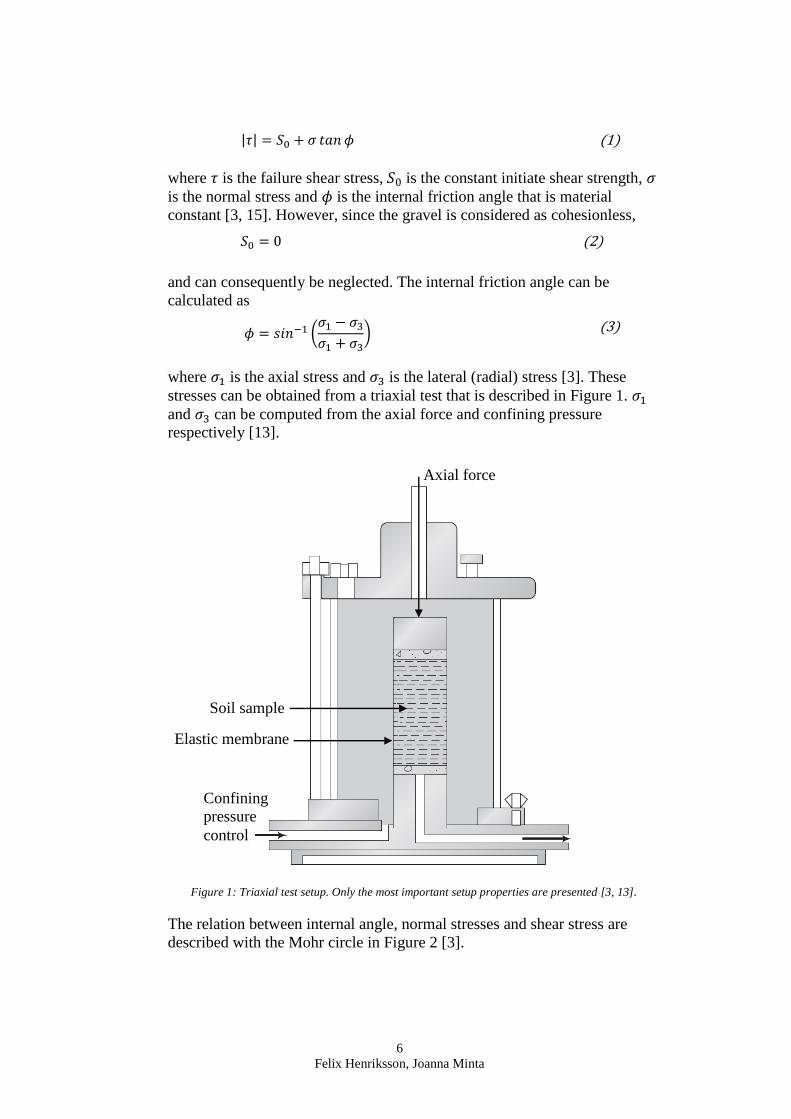
where 𝜎1 is the axial stress and 𝜎3 is the lateral (radial) stress [3]. These
stresses can be obtained from a triaxial test that is described in Figure 1. 𝜎1
and 𝜎3 can be computed from the axial force and confining pressure
respectively [13].
Figure 1: Triaxial test setup. Only the most important setup properties are presented [3, 13].
The relation between internal angle, normal stresses and shear stress are
described with the Mohr circle in Figure 2 [3].
Elastic membrane
Soil sample
Axial force
Confining
pressure
control

7
Felix Henriksson, Joanna Minta
Figure 2: Mohr circle that illustrates the relation between internal friction angle, shear stress and
normal stress [3].
The normal stress, 𝜎, acts perpendicularly to a shear plane, and the shear
stress, 𝜏, is acting parallel with this shear plane. The last parameter, internal
friction angel 𝜙, is dependent on material characteristics such as shape,
packing density and friction of the soil particles [3].
Another important property is the porosity
𝑛 =
𝑉𝑉
𝑉𝑇= 1 −
𝜌𝑏
𝜌𝑔 (4)
where 𝑉𝑉 is the volume of void and the volume of material is 𝑉𝑇 . In the
second expression it is stated by the bulk density, 𝜌𝑔, and grain density, 𝜌𝑏
[3].
The degree of packing between the loosest and densest state of course-
grained soils can be described with the porosities, maximum, 𝑛𝑚𝑎𝑥,
minimum, 𝑛𝑚in, and actual, 𝑛, as the relative density 𝐷𝑟 [3]
𝐷𝑟 =
(𝑛𝑚𝑎𝑥 − 𝑛)(1 − 𝑛𝑚𝑖𝑛)
(𝑛𝑚𝑎𝑥 − 𝑛𝑚𝑖𝑛)(1 − 𝑛) (5)
This aspect is strongly correlated with the strength of the soil [3]. A looser
soil is weaker than a denser soil. Two different possible density states with
the same soil are presented in Figure 3.
𝜎1 𝜎3
𝜏
𝜙
𝜎𝑚
normal stress, 𝜎
shea
r st
ress
, 𝜏

8
Felix Henriksson, Joanna Minta
Figure 3: Different density states for the same soil. The left state is loose state and the right state is
dense. (a) represents a plane between the particle rows [13].
2.1.1.2 Gravel
Gravel is a granular material that consists of a large amount of single grains
in contact with each other [3]. Displacements of the grains are performed by
contact forces from other grains or external elements. Moreover, the contact
forces depend on the bulk properties that in turn depend on the particle
properties of the gravel such as normal stiffness, shape, friction and density.
The order of the grains is also important and this is affected by the porosity,
interlocking between grains and distribution of grain size [3]. The gravel can
be considered both as a fluid or a solid dependent on its state determined by,
for instance packing density and flow velocity. However, the dilation
behavior of gravel, during certain conditions, in contrast to solids and fluids
are different. For instance, formations of heaps are only present in situations
including gravel or other granular material.
Examples of cohesionless gravel properties without rotational degrees of
freedom are presented in Table 1, some of the properties will be explained in
section 2.2.
Table 1: Properties of cohesionless gravel without rotational degrees of freedom [3].
Property Value Unit
normal stiffness, �̂� 100 MPa
tangential stiffness, 𝑘𝑇 107 N/m
porosity 0.41 -
confining pressure, 𝜎3 20 kPa
local friction coeffictient, 𝜇 0.3 -
2.2 Discrete Element Method
The Discrete Element Method (DEM) is a numerical method that is used to
analyze the behavior of, for instance, particulate material. It was first
presented for this type of application in 1979 of Cundall and Strack [7].
Although it was developed in the 1970s, applications similar to the one
studied in this thesis have been infeasible until the last couple of years. The
increased use is a result of the availability of cluster computers and better
algorithms distributing the computations.
This development has enabled modeling of granular material with DEM
where Newton’s second law can directly be applied [16]. Additionally, it is

9
Felix Henriksson, Joanna Minta
worth pointing out that by using a set of discrete particles instead of grids it
is possible to avoid the numerical problems with mesh distortion. In DEM
each particle is treated individually. The frequency of collision and duration
of contact with neighbor particles can be computed if path and velocity of
each particle has is known [7, 17].
The term discrete element method refers to any computational models that
allow finite displacements and rotations of discrete bodies and recognizes
new contacts automatically as the calculation progress [8]. The Discrete
Element Method is a numerical method and algorithm allowing calculation
of the physical properties of a large amount of objects in motion [16]. The
calculation algorithm consists of two independent steps that are solving two
kinds of equations. In the first time step the law of motion is applied to each
particle to calculate displacements of elements which are a result of the
external forces acting on it. The second step applies the force-displacement
law which calculates the forces acting on the interacting elements. A
schematic view of the algorithm is shown in Figure 4.
Figure 4: Calculation cycle for DEM [16].
Law of Motion
By taking dilation of elements into account it can be shown that each
discrete element can undergo both translational and rotational motion. The
translational motion of the center of the mass is described with respect to its
position, 𝑥𝑖 , velocity, �̇�𝑖 and acceleration, �̈�𝑖. The rotational motion of the
particle is described with respect to its angular velocity, �̇�𝑖 and angular
acceleration,ω̈𝑖 [7, 16]. Hence, the equation of motion can be expressed as
the two vector equations
Law of Motion
(applied to each particle)
resultant force +moment
Force-Displacement Law
(applied to each contact)
relative motion
constitutive law
update particle + wall positions and set of contacts
contact forces

10
Felix Henriksson, Joanna Minta
𝐹𝑖 = 𝑚𝑖�̈�𝑖 (6)
𝑀𝑖 = 𝐼𝑖𝜔𝑖 × 𝜔𝑖 + 𝐼𝑖�̇�𝑖 (7)
where 𝐹𝑖 is the resultant force on particle 𝑖, 𝑀𝑖 is the rotational moment on
particle 𝑖, 𝑚𝑖 is the mass and 𝐼𝑖 is the inertia tensor.
The Force-Displacement Law
The force-displacement law updates the contact forces arising from the
relative motion between the particles. The contact condition between two
particles is shown in Figure 5. The contact point, 𝑥𝑖, located on a contact
plane is defined by a unit normal vector, 𝑛𝑖. The force-displacement law
relates via the normal and shear stiffness at the contact, normal component
acting in the direction of the normal vector and a shear component acting in
the plane to the corresponding components of the relative motion [16].
Besides the forces at the contact point, the contribution to moment from a
contact point can be calculated by
𝑀𝑖 = 𝐹𝑖 × 𝑅𝑖 (8)
where 𝐹 is the force vector, 𝑅 is the contact position vector and 𝑖 indicates
the index of the contact points.

11
Felix Henriksson, Joanna Minta
Figure 5: Contact law between two particles.
2.2.2.1 Normal Forces
From basic assumptions, the elements are treated as rigid bodies and are
allowed to overlap each other. The normal forces follow the assumption of
Hertzian contact. Figure 6 shows the overlap, 𝛿, at the contact point of two
spheres and the radius of the contact area, 𝑎 [3].

12
Felix Henriksson, Joanna Minta
Figure 6: The penetration 𝛿 at the contact of two spheres with radii 𝑟1 and 𝑟2 [3].
To calculate the overlap, 𝛿𝑖𝑗, between two spherical particles, i and j, it is
necessary to know their respective positions 𝑥𝑖 and 𝑥𝑗 and radiuses 𝑟𝑖 and 𝑟𝑗
𝛿𝑖𝑗 = 𝑟𝑖 + 𝑟𝑗 − ‖𝑥𝑖 − 𝑥𝑗‖ (9)
The repulsive contact force is calculated when 𝛿𝑖𝑗 > 0 [3, 14].
For linear cases, a simple linear spring and dashpot models are applied
𝐹𝑁,𝑖𝑗 = 𝑘𝑁𝛿𝑖𝑗 + 𝑑𝑁�̇�𝑖𝑗 (10)
where 𝐹𝑁 is normal force, 𝑘𝑁 is normal stiffness and 𝑑𝑁 is normal damping
coefficient. The normal forces could then be described as the vector
𝑓𝑁,𝑖𝑗 = 𝐹𝑁,𝑖𝑗𝑛 (11)
where
𝑛 =𝑥𝑗 − 𝑥𝑖
‖𝑥𝑗 − 𝑥𝑖‖ (12)
is a normal to the contact point. For most cases, a fixed 𝑘𝑁 is assumed for all
contacts. However, in this case the applied stiffness is calculated due to the
deformation of an elastic rod with cross-section 𝐴, Young’s modulus �̂�, and
length 𝑙 that is connecting the particles at the center points [3]
𝑘𝑁,𝑖𝑗 =
�̂�𝐴𝑖𝑗
𝑙𝑖𝑗=
�̂��̅�2𝜋
2𝑟𝑖𝑗=
𝜋
2�̂��̅� (13)
where the average radius is
�̅� =
(𝑟𝑖 + 𝑟𝑗)
2 (14)
The damping coefficient is not important in this thesis. Nevertheless, with a
given coefficient of restitution it is possible to derive them [3, 14]. In this
thesis the normal damping is set to 0.3 between the particles.

13
Felix Henriksson, Joanna Minta
2.2.2.2 Tangential Forces
When two particles initially get in contact, the contact points 𝑋𝐶,1 and 𝑋𝐶,2
are positioned in their particle coordinate systems, these positions are stored.
A later position is showed in Figure 7. The denotation of the particles as 1
and 2 is arbitrary, but must be the same while the particles remain in contact
[3].
Figure 7: The tangential spring vector 𝜉𝑇 caused by rotation of two particles [3].
The contact points do not coincide in the successive simulation steps as long
as the contact points strictly undergo a relative displacement. This is shown
in Figure 7 where the contact points are on the way away from each other
[3].
In order to determine the tangential friction deformation, every simulation
step consists of transformation of the contacts points to the global coordinate
system where 𝑥𝑖 the center of the particles and 𝑅𝑖 the rotational matrix that
describes the orientations of the particles [14]
𝑥𝐶,1 = 𝑥1 + 𝑅1𝑋𝐶,1 (15)
𝑥𝐶,2 = 𝑥2 + 𝑅2𝑋𝐶,2 (16)
The relative deformation between these two points, is computed from
𝜉𝑇 = 𝑥𝐶,2 − 𝑥𝐶,1 (17)
and to get the tangential deformation, this vector is projected onto the
tangential plane
𝜉𝑇 = 𝜉𝑇 − (𝜉𝑇 ∙ 𝑛)𝑛 (18)
Afterwards the tangential force is computed from
𝑓𝑇 = −𝑘𝑇𝜉𝑇 − 𝑑𝑇�̇�𝑇 (19)
where 𝑘𝑇 is the tangential stiffness, 𝑑𝑇 is the tangential damping coefficient
and �̇�𝑇 is the relative tangential velocity of the particles.

14
Felix Henriksson, Joanna Minta
Slipping will be present if the tangential force exceeds the limit
𝐹𝑇 = 𝜇𝐹𝑁 (20)
where 𝜇 is the local friction coefficient.
To account for the state of slipping, the tangential spring is reset to
𝜉′𝑇 =
𝜇𝐹𝑁
𝑘𝑇∙
𝜉𝑇
‖𝜉𝑇‖ (21)
and the new tangential spring length is used to update the contact points
𝑥′𝐶,1 = 𝑥𝑎 +
𝜉′𝑇
2 (22)
𝑥′𝐶,2 = 𝑥𝑎 −
𝜉′𝑇
2 (23)
where the current contact point is computed from
𝑥𝑎 = 𝑥1 +𝑟1
𝑟1 + 𝑟2
(𝑥2 − 𝑥1). (24)
The actuation point does not have to be located on the surface of the spheres
due to a possible overlap 𝛿. For the next simulation step the new contact
points are stored in the local coordinate system
𝑋′𝐶,1 = 𝑅𝑇(𝑥𝐶,1′ − 𝑥1) (25)
𝑋′𝐶,2 = 𝑅𝑇(𝑥𝐶,2′ − 𝑥2) (26)
Application of the tangential contact forces onto the mass center of the
particle is done according to
𝑓1 = 𝑓𝑇 (27)
𝑓2 = −𝑓𝑇 (28)
Also the torques
𝑡1 = (𝑥𝑎 − 𝑥1) × 𝑓𝑇 (29)
𝑡2 = −(𝑥𝑎 − 𝑥2) × 𝑓𝑇 (30)
From the contact forces are applied to the mass center. The simulation
influence of different friction coefficients for static and kinetic friction is
negligible, while it is strictly necessary for the results if a slow or quasi-
static granular material should account for sticking friction [3, 14].
Determination of Forces Acting on the Bucket
During the last few years the forces exerted between soil and tool have been
studied in different fields of engineering. At present time, two methods exist
15
Felix Henriksson, Joanna Minta
to calculate these forces, analytical and numerical. However, analytical
methods are limited to simple tool geometries and trajectories.
Numerical methods are classified into continuum or discrete methods where
discrete methods are more common due to their higher numerical efficiency
and simpler applicability. To be able to simulate material flow with a
numerical method, the method has to allow low dense, fast particle flow and
large displacements [3].
Bucket-filling is one application where numerical methods are used for
granular flow [19, 20]. Due to this, most of the investigating of draft forces
is based on the DEM, since the method is feasible for these applications the
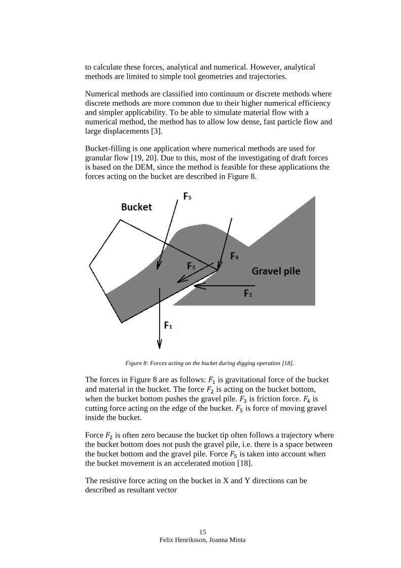
forces acting on the bucket are described in Figure 8.
Figure 8: Forces acting on the bucket during digging operation [18].
The forces in Figure 8 are as follows: 𝐹1 is gravitational force of the bucket
and material in the bucket. The force 𝐹2 is acting on the bucket bottom,
when the bucket bottom pushes the gravel pile. 𝐹3 is friction force. 𝐹4 is
cutting force acting on the edge of the bucket. 𝐹5 is force of moving gravel
inside the bucket.
Force 𝐹2 is often zero because the bucket tip often follows a trajectory where
the bucket bottom does not push the gravel pile, i.e. there is a space between
the bucket bottom and the gravel pile. Force 𝐹5 is taken into account when
the bucket movement is an accelerated motion [18].
The resistive force acting on the bucket in X and Y directions can be
described as resultant vector

16
Felix Henriksson, Joanna Minta
𝐹𝑋 = 𝐹3𝑋 + 𝐹4𝑋 + 𝐹5𝑋 (31)
𝐹𝑌 = 𝐹1𝑌 + 𝐹3𝑌 + 𝐹4𝑌 + 𝐹5𝑌 (32)
DEM Implementation
The general numerical algorithm of DEM is shown in Figure 9.
Figure 9: DEM numerical algorithm [21].

17
Felix Henriksson, Joanna Minta
To start a DEM simulation, particles are placed into a container and contact
detection search is performed to achieve the contact between all single
particles. From this, contact forces and particle motion can be calculated
according to section 2.1.1 and 2.2.2 [7].
2.2.4.1 Time Step Size
DEM uses an explicit time integration scheme and the stability of the
solutions with explicit time integration is strongly influenced by the time
step size [22]. The time step should be smaller than its critical value which is
generally defined as
∆𝑡𝑐𝑟𝑖𝑡 =
2
𝜔𝑛 (33)
where 𝜔𝑛 is the maximum eigenfrequency of the system. For DEM setup the
largest eigenfrequency could be estimated from
𝜔𝑛 = 𝑐1√𝑘
𝑚 (34)
where 𝑐1 is a constant that treats the impact of contacts, 𝑘 is the normal
stiffness and 𝑚 is the smallest mass of a particle. This implies that a stiffer
system decreases the critical time step and increases the total execution time.
2.2.4.2 DEM modeling of Granular Material
In geotechnical applications the size of particles ranges over numerous
order, for example, gravel has 10−2 m particle size. Although, it is not
possible at present time to model the micro properties of real soil in DEM
simulation, heterogeneous soil can still be modeled by adjusting the
parameters accordingly [3]. The real particle shape is not feasible to model
at current state and DEM simulations only consider a relative small number
(~100000) of particles to achieve a practical simulation [7].
Since only a single value, the radius, is required to define the geometry of a
spherical or circular particle, most of the DEMs implement disks or
spherical elements for 2D- and 3D-models respectively. It should be
mentioned that disks and spheres can easily rotate or roll, that is likely to
occur in granular material during shear deformation. However, it is possible
to model shapes that are more complicated as well but this will increase the
intensity of the computations since it will be much more problematic to
detect contacts and calculate the forces and torques in the contact points.
The contacts of real particles may appear in many different ways in contrast
to a spherical particle that only has one uniform surface. An irregularly
shaped particle consists of corners, edges and surfaces which will cause
different types of contacts [23].
18
Felix Henriksson, Joanna Minta
In a DEM simulation, it is required to simplify the model of the granular
material, because it is not possible to transfer properties like shape, size
distribution, consolidation state, and friction between grains exactly to the
DEM model [3]. To exemplify, the simulation of one million non-spherical
particles is not reasonable to be performed by a single processor; this
operation requires a lot of hours [7]. Hence, the gravel is modeled as rigid
spherical particles with three degrees of freedom i.e. x, y z, without rotation.
This will change the behavior of the model, but the forces will still be
realistic and similar to results of simulations with rotational particles [3].
DEM Software
At present time, a couple of software for DEM simulation exists. STAR-
CCM+ is based on the Lagrangian Multiphase model. Other examples are
EDEM and Newton. All software are very similar, they are quick and
accurately simulates three-dimensional granular flow behavior of different
shaped and sized spherical particles. The exception is Rocky that possesses
the ability to simulate true non-spherical particles.
GRAPE, developed by Fraunhofer ITWM, can perform simulations of
granular material including characterization of the granular material. It treats
macroscopic properties of granular material, measured in laboratory
experiments e.g. triaxial tests. The software allows prediction of the
behavior of granular material.
2.3 Multibody Systems
Multibody systems (MBS) consist of interconnected subsystems [24]. These
subsystems are defined as components, rigid bodies or substructures. Single
parts in these subsystems can be treated both as rigid or flexible bodies. To
create a system, these bodies are jointed to constrain the motion. Dependent
on the linking at the actual object, a suitable joint is selected. This will allow
the jointed parts to move with respect to each other. The motion allowed by
the joint could be rotational, translation or a combination.
Typical applications of MBS are for instance aircrafts, vehicles and various
mechanical systems [24]. To achieve a system that corresponds to reality,
knowledge about the behavior of different subsystems is required.
Simulation of Multibody Systems
Simulation of MBS is performed by software where a model is built.
Nowadays, a couple of MBS software are available on the market, for
example Adams, LMS Motion, Pro/MECHANICA or Working Model.
19
Felix Henriksson, Joanna Minta
Analysis of motion is fundamental during product design since it is
important to understand the interaction of elements, both with each other and
the surrounding environment [25].
In this thesis simulation of Multibody System is performed with Adams. To
create accurate models in Adams, it is necessary to integrate components
such as hydraulics, pneumatics, electronic, control system technologies and
mechanical components [4]. Thus, the model can be simulated with high
precision which allows valid designs at an early stage.
2.4 Simulation of Dynamic Systems
Modeling and simulation of dynamics can be performed by Simulink, which
is an integrated tool in Matlab, developed by MathWorks [11]. A Simulink
model can be created from the built-in block library that contains different
blocks, which assembled together, can represent engineering systems. For
instance, the blocks can perform derivatives or integrations, both continuous
and discrete states, to describe a system. It is also possible to modify these
blocks or to add hand-written ones from Matlab. These blocks are eventually
linked with mathematical relations to create a dynamic system with different
subsystems.
Simulink also contains a graphical interface where schematic views can be
obtained of the investigated dynamic model [11]. It is also a very efficient
tool to use when different software are used to perform co-operating
simulations.

20
Felix Henriksson, Joanna Minta
3. Method
The study in this thesis will be performed using a quantitative method. The
method is considered quantitative since the results will be achieved using
simulations and analysis of the results. The results are numerical and
consequently quantitative. The results from the simulations will be analyzed
to establish the most feasible trade-off between computational time and
accuracy of the results.
To perform the simulations in this thesis, an existing computational model
from Volvo CE will be used. The model consists of three parts, 1) a Discrete
Element Method (DEM) to model the gravel with the software GRAPE, 2)
the wheel loader built in Adams as a Multibody system model and 3) the
Simulink model that provides the connection between Adams and GRAPE.
3.1 Total Simulation Model
The major properties that are relevant to study in this thesis are specified in
Table 2, where the values listed are for a model setup considered as baseline.
These properties will be explained more detailed in the following sections.
Table 2: Total model properties and their baseline values.
Property Value Unit
Collision detection interval 5 ∙ 10−4 [s] Co-simulation interval 2 ∙ 10−3 [s]
Friction coefficient 0.25 -
Normal stiffness 4 ∙ 107 [N/m]
Discrete Element Method
The gravel pile in this study is modeled with DEM using the software
GRAPE from Fraunhofer ITWM. Simplifications are applied to allow
reasonable solution time i.e. only spherical elements with three translational
degrees of freedom, x, y and z, are used.
The collision detection interval is the time that proceeds between successive
searches of potential candidates for contacts between particles during
simulations. Consequently, smaller collision detection interval will lead to
an increased number of global searches and thus, longer simulation time.
Hence, as large interval as possible with retained result accuracy is desired
to be used. The initial value in the model is 0.0005 s.
The influence of the friction coefficient and normal stiffness are the gravel
particle parameters that are believed to have greatest influence on output
results. These parameters are important to consider since they might change
21
Felix Henriksson, Joanna Minta
if another material is handled. However, only the normal stiffness will be
investigated due to the limitation of the thesis.
The material that the DEM model is supposed to represent is crushed stones
and such material is intended to be handled with a re-handling bucket, as
applied in this thesis.
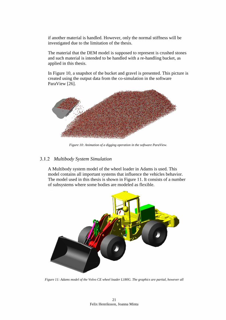
In Figure 10, a snapshot of the bucket and gravel is presented. This picture is
created using the output data from the co-simulation in the software
ParaView [26].
Figure 10: Animation of a digging operation in the software ParaView.
Multibody System Simulation
A Multibody system model of the wheel loader in Adams is used. This
model contains all important systems that influence the vehicles behavior.
The model used in this thesis is shown in Figure 11. It consists of a number
of subsystems where some bodies are modeled as flexible.
Figure 11: Adams model of the Volvo CE wheel loader L180G. The graphics are partial, however all

22
Felix Henriksson, Joanna Minta
relevant mechanical systems are implemented.
The bucket, shown in Figure 11, is a re-handling bucket and has a smooth
shape without teeth. The selection of bucket-type in a real application is very
much dependent on what material should be handled. A wrong selection will
increase the fuel consumption and wear of the bucket significantly. If
another type of bucket would have been used in the simulations the result
would have been different.
Simulink
The Simulink model provides the connection between the different software.
It also contains the powertrain and hydraulics of the wheel loader. However,
these are not considered in this thesis. An overview of the Simulink model at
global level is showed in Figure 12.
Figure 12: Simulink model.
When performing the co-simulations, the Adams model is exported and
loaded into the Simulink model. After Simulink has finished the simulation,
the results will be read into to Adams where the result can be animated and
analyzed.
3.2 The Assembled Model
During the co-simulations the wheel loader is actuated with a prescribed
motion that performs a digging operation. When running the simulation,
Adams sends displacements, angles, velocities and angular velocities of the
wheel loader bucket to Simulink which processes these states and forwards
them to a DEM-solver. The DEM-solver is executed on a Linux-cluster and

23
Felix Henriksson, Joanna Minta
without access to such computational power, these computations would be
practically unsolvable.
The outputs of the DEM-solver are three forces and three torques in the
global x, y and z direction. These forces and torques are accordingly sent
back to Adams where they are applied at a reference point of the wheel
loader bucket. Adams then computes new states of motion of the bucket due
to the new acting forces. These are then sent to the DEM-solver through
Simulink and this process is repeated until the simulation end time is
reached. An overview of how the models are assembled is showed in Figure
13.
Figure 13: Overview of the assembled model [27].
The time that passes between two successive communications from the
Adams model and DEM-solver and vice-versa is termed co-simulation
communication interval. This is a highly relevant property and is controlled
by a parameter in the Simulink model that is possible to modify. Its initial
value is 0.002 s. In Figure 14, the co-simulation interval is described where
the top axis represents the time of the DEM-solver and each mark on it
represents a time step that is constant trough the complete simulation. The
lower axis represents the Adams model, where the time step size is not
constant. The solver decreases the time step when the computation reaches a
critical state and increases the time step when that is suitable, i.e. an adaptive
time stepping algorithm [28].

24
Felix Henriksson, Joanna Minta
Figure 14: Explanation of the co-simulation interval.
The vertical arrows represent time instances when Simulink reaches a
communication time step and consequently where the DEM-solver and
Adams exchange data. The diagonal arrows represent the step until the next
communication event. In this case, the communication interval is four times
the DEM-solver time step. This communication interval has to be a multiple
of the DEM-solver step size since a fixed time stepping scheme is used.
The influence of step size is investigated by simulations with different
values. Since a smaller time step will increase the amount of steps to reach
the end time, it has a strong impact on the simulation time.
3.3 Collection of Data
This section describes how the data collection of this thesis is performed.
The data received from co-simulation are compared with experimental data
measured at Volvo CE a few years ago.
Simulated Data
The data is extracted from the co-simulations between GRAPE, Adams and
Simulink. To obtain a proper data set, various simulations are performed
with different setups.
Since the simulations produce a huge amount of output data, an Adams
command assists extraction of relevant results for this thesis i.e. the resulting
pin forces defined in Figure 15. These results are eventually processed with
a Matlab script that plots the requested results.
simulation time
DEM-solver
Adams model

25
Felix Henriksson, Joanna Minta
Figure 15: Bucket modeled in Adams. The resulting forces in the pins attached in the specified
pinholes during digging operation are investigated in this thesis.
The direction of the pin forces are measured in the bucket co-rotational
coordinate system explained in Figure 16. In Figure 17, the resultant forces
in the bucket reference point, A-pin and J-pin are visualized.
Figure 16: Illustration of how the coordinate system for the bucket is operating, i.e. it is following an
eventual angular displacement of the bucket.
AL
AR J
x
z

26
Felix Henriksson, Joanna Minta
Figure 17: Visualization of resultant forces during digging operation.
Measured Data
The measured data utilized in this thesis are from previous experiments
performed by Volvo CE. For instance the lift and tilt cylinder motions are
measured and these are plotted in Figure 18 for one cycle.
a) b)
Figure 18: Plots of the measured lift cylinder motions, a), and tilt cylinder motions, b).
Forces in the tilt and lift cylinders, specified in Figure 19, are measured
during experiments. Besides these forces, pin forces and angles between
certain parts in the structure in Figure 19 are measured. To show all
measured entities in a figure is complicated and this is why they are not
specified.
27
Felix Henriksson, Joanna Minta
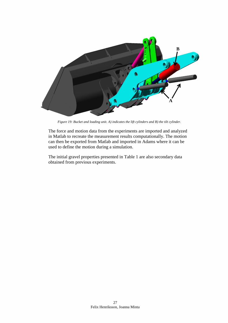
Figure 19: Bucket and loading unit. A) indicates the lift cylinders and B) the tilt cylinder.
The force and motion data from the experiments are imported and analyzed
in Matlab to recreate the measurement results computationally. The motion
can then be exported from Matlab and imported in Adams where it can be
used to define the motion during a simulation.
The initial gravel properties presented in Table 1 are also secondary data
obtained from previous experiments.
A
B

28
Felix Henriksson, Joanna Minta
4. Results and Analysis
In this section the results will be presented and analyzed. In section 4.1, the
different simulation setups are defined and in the coming sections the
measurement and simulation results are presented.
4.1 Simulation Setups
Table 3 presents the simulation-setups with altering values for collision
detection interval and co-simulation interval. These will be analyzed in
feasible sets in the following sections. During the analyses, the first 15 s of a
short cycle loading is simulated. This time covers the bucket-filling phase.
The simulation time presented in Table 3 corresponds to the time it takes
execute the simulation. A complete list of simulation setups is available in
Appendix 1.
Table 3: Investigated test setups.
Sim ID Collision Detection
Interval [s]
Co-Sim
Interval [s]
Normal
Stiffness [Pa]
Simulation
Time [s]
Sim_0_Initial 0.0005 0.002 4.0E+07 4800
Sim_001_01 0.0001 0.0005 4.0E+07 16500
Sim_002 0.0005 0.001 4.0E+07 6700
Sim_003 0.0004 0.0008 4.0E+07 6900
Sim_004 0.0004 0.002 4.0E+07 5100
Sim_005_01 0.0002 0.0008 4.0E+07 9500
Sim_006 0.0002 0.002 4.0E+07 6900
Sim_007 0.0001 0.0006 4.0E+07 15500
Sim_008 0.0002 0.001 4.0E+07 8600
Sim_009 0.0001 0.001 4.0E+07 12600
Sim_010 0.0001 0.002 4.0E+07 10700
Sim_011 0.0002 0.0006 4.0E+07 11400
Sim_012 0.0003 0.0006 4.0E+07 10100
Sim_013 0.0001 0.0004 4.0E+07 19000
Sim_014_01 0.0002 0.0004 4.0E+07 14600
Sim_015 0.0001 0.0002 4.0E+07 30100
4.2 Baseline Simulation Compared to Measurement
In this section measurement data is compared to simulation results from
Sim_0_Initial. Figure 20-22 show the pin forces acting on the bucket in x
and z directions during the bucket filling phase. For clarification of force
location and definition of the coordinate system, see Figure 15 and 16.

29
Felix Henriksson, Joanna Minta
Figure 20: Compared plots from measurement data and simulation of the right A-pin force.
Figure 21: Compared plots from measurement data and simulation of the left A-pin force.
30
Felix Henriksson, Joanna Minta
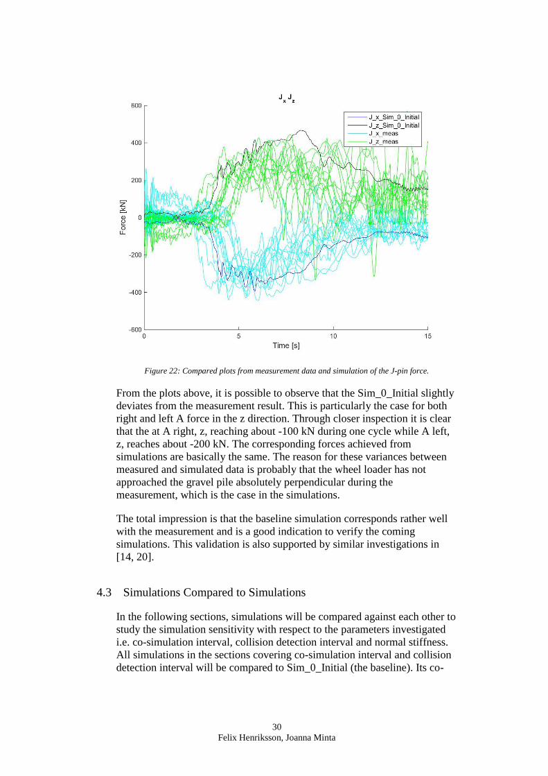
Figure 22: Compared plots from measurement data and simulation of the J-pin force.
From the plots above, it is possible to observe that the Sim_0_Initial slightly
deviates from the measurement result. This is particularly the case for both
right and left A force in the z direction. Through closer inspection it is clear
that the at A right, z, reaching about -100 kN during one cycle while A left,
z, reaches about -200 kN. The corresponding forces achieved from
simulations are basically the same. The reason for these variances between
measured and simulated data is probably that the wheel loader has not
approached the gravel pile absolutely perpendicular during the
measurement, which is the case in the simulations.
The total impression is that the baseline simulation corresponds rather well
with the measurement and is a good indication to verify the coming
simulations. This validation is also supported by similar investigations in
[14, 20].
4.3 Simulations Compared to Simulations
In the following sections, simulations will be compared against each other to
study the simulation sensitivity with respect to the parameters investigated
i.e. co-simulation interval, collision detection interval and normal stiffness.
All simulations in the sections covering co-simulation interval and collision
detection interval will be compared to Sim_0_Initial (the baseline). Its co-

31
Felix Henriksson, Joanna Minta
simulation interval is 0.002 s, collision detection interval 0.0005 s and the
simulation time is 4800 s to simulate the initial 15 s.
In this section only the forces in the left A pinhole will be presented. The
right A pin forces are practically identical to left A pin forces. The J forces
are also considered but do not add anything particular. The J force plots are
available in Appendix 2.
Co-Simulation Interval
In Figure 23-27, plots with different co-simulation intervals are presented.
Sim_0_Initial (the baseline), has the largest co-simulation interval.
The presented results have constant normal stiffness and collision detection
interval. Since the selection of collision detection interval depends on the co-
simulation interval as explained in Figure 14, the co-simulation interval
results will be presented in different sets. In each set, the collision detection
interval is the same.
4.3.1.1 Collision Detection Interval constant to 0.0005 s
In Figure 23, Sim_002 is compared to Sim_016 and their co-simulation
intervals are 0.001 s and 0.0005 s, respectively. This decreased co-
simulation interval causes an increased simulation time from 6700 s to
10200 s.

32
Felix Henriksson, Joanna Minta
Figure 23: Comparison of Sim_002 and Sim_016.
It is clear that the simulations match each other rather good. All simulations
have distinct force amplitudes in the x direction, which is the upper part of
the plot. Some oscillation appears during the final three seconds, which is
difficult to explain since the bucket is not in contact with the gravel pile at
that time. These are plotted in detail in Figure 24.

33
Felix Henriksson, Joanna Minta
Figure 24: Comparison of Sim_002 and Sim_016, enlarged to clarify force oscillations.
In Figure 24 it is observed that some oscillations appear during the last few
second. Since all plots so far have indicated large force amplitudes and some
oscillations, the coming simulations will be run with lower collision
detection interval to be able to reduce the co-simulation interval and thus,
the oscillation and force peaks.
4.3.1.2 Collision Detection Interval constant to 0.0002 s
In Figure 25 Sim_005_01 (0.0008 s), Sim_006 (0.002 s), Sim_008 (0.001 s)
and Sim_014_01 (0.0004 s) are compared.

34
Felix Henriksson, Joanna Minta
Figure 25: Comparison of Sim_005_01, Sim_006, Sim_008 and Sim_014_01.
All simulations show good agreement with the baseline, although some large
force amplitudes are present during 4-7 s. On the other hand, the previously
presented oscillations in the final seconds have disappeared.
The force amplitudes for Sim_005_01 are a bit lower than in Sim_006 and
the baseline and is a results of the reduced co-simulation interval. The
smoothest force plot is Sim_014_01, i.e. the simulation with smallest co-
simulation interval which also led to a longer simulation time, 14600 s.
4.3.1.3 Collision Detection Interval constant to 0.0001 s
The co-simulation detection interval is constant to 0.0001 s in the following
comparisons. In Figure 26 Sim_007 (0.0006 s), Sim_009 (0.001 s) and
Sim_010 (0.002 s) are compared.

35
Felix Henriksson, Joanna Minta
Figure 26: Comparison of Sim_007, Sim_009 and Sim_010.
The plots are quite similar to each other and the baseline. Some oscillating
force ranges are present during 4-7 s.
In Figure 27, Sim_001_01 (0.0005 s), Sim_013 (0.0004 s) and Sim_015
(0.0002 s) are compared.

36
Felix Henriksson, Joanna Minta
Figure 27: Comparison of Sim_001_01, Sim_013 and Sim_015.
The oscillating forces has somewhat smaller in ranges Sim_001_01 and
Sim_015 than in Sim_013. It is considerably unexpected that Sim_013 has
higher amplitudes than Sim_001_01 since its co-simulation interval is
smaller. This implies that it is more complex to predict the behavior since it
is not certain that a shorter co-simulation interval would give a smoother
solution.
4.3.1.4 Summary
To summarize the results of the simulations with constant collision detection
interval and alternating co-simulation interval it is concluded that a shorter
co-simulation interval results in smoother forces generally, although there
are exceptions, for instance Sim_013. It is also clear that a decreased co-
simulation interval increases the simulation time. All simulations are
corresponding well to baseline. In Table 4, the different setups in this
section are summarized.

37
Felix Henriksson, Joanna Minta
Table 4: Simulation setups investigated in section 0.
Sim ID Collision Detection
Interval [s]
Co-simulation
Interval [s]
Simulation
time [s] Comment
Sim_0_Initial 0.0005 0.002 4824 Large force peaks
Sim_002 0.0005 0.001 6706.5 Large force peaks
Sim_016 0.0005 0.0005 10211 Large force peaks
Sim_006 0.0002 0.002 6921.6 Large force peaks
Sim_008 0.0002 0.001 8581 Medium force peaks
Sim_005_01 0.0002 0.0008 9532.6 Medium force peaks
Sim_014_01 0.0002 0.0004 14641 Low force peaks
Sim_010 0.0001 0.002 10731 Medium force peaks
Sim_009 0.0001 0.001 12572 Large force peaks
Sim_007 0.0001 0.0006 15501 Large force peaks
Sim_001_01 0.0001 0.0005 16544 Low force peaks
Sim_013 0.0001 0.0004 19015 Large force peaks
Sim_015 0.0001 0.0002 30129 Low force peaks
Considering the simulation times and the computed forces, Sim_005_01 and
Sim_014_01 are considered to be the most suitable for investigation
regarding normal stiffness.
Collision Detection Interval
The collision detection interval has been investigated with the same method
as used for the communication simulation interval in the previous section.
4.3.2.1 Co-Simulation Interval constant to 0.002 s
In Figure 28 Sim_004 (0.0004 s), Sim_006 (0.0002 s) and Sim_010 (0.0001
s) are compared where their collision detection intervals are specified in the
parentheses.

38
Felix Henriksson, Joanna Minta
Figure 28: Comparison of Sim_004, Sim_006 and Sim_010.
All simulations indicate some force oscillations. In Sim_004, oscillations
appear from 7 s to 10 s. In Sim_004, Sim_006 and Sim_010 oscillations
appears in the end of the simulation, although small compared to
Sim_0_Initial. Sim_004 and Sim_006 have the largest span in collision
detection interval compared to the other simulations showed in Figure 28.
Hence, these plots are deviating more from each other. It is possible to
observe that Sim_006 has larger force ranges in x and z direction than
Sim_010 during 4-8 s.
4.3.2.2 Co-Simulation Interval constant to 0.0006 s
In Figure 29, Sim_007 (0.0001 s), Sim_011 (0.0002 s) and Sim_012 (0.0003
s) are compared.

39
Felix Henriksson, Joanna Minta
Figure 29: Comparison of Sim_007, Sim_011 and Sim_012.
In Sim_011 and Sim_012 the results deviate slightly in x direction, which is
the upper part, but in z direction they are quite similar. Towards the end of
the simulation time, some small oscillations appear in both x and z direction.
In Sim_011 it is easy to observe some oscillations close to the end
simulation time. If Sim_007 is compared to Sim_011 and Sim_012, there is
an offset in time, otherwise they are matching each other rather good. The
simulation time increases as the collision detection interval decreases.
4.3.2.3 Co-Simulation Interval constant to 0.0004 s
In Figure 30, Sim_013 is compared with Sim_014_01. The collision
detection interval for Sim_013 is 0.0001 s and for Sim_014 is 0.0002 s.

40
Felix Henriksson, Joanna Minta
Figure 30: Comparison of Sim_013 and Sim_014_01.
Compared to Sim_014_01, Sim_013 has larger force ranges in 4-8 s,
otherwise they are quite similar. We also observe that only very low
amplitude oscillations appear in the last three seconds. Sim_014 has smaller
force amplitudes during 3-7 s, than Sim_0_Initial and Sim_013. The
simulation time increase from 14641 s in Sim_014 to 19015 s in Sim_013.
4.3.2.4 Summary
The results of the simulation with constant co-simulation interval and
alternating collision detection interval demonstrate that a decreased collision
detection interval increases the simulation time. All simulations match each
other and the baseline rather good. The different setups and some short
comments are presented in Table 5.

41
Felix Henriksson, Joanna Minta
Table 5: Simulation setups investigated in section 4.3.2.
Sim ID
Collision
Detection
Interval [s]
Co-
simulation
Interval [s]
Simulation
time [s] Comment
Sim_0_Initial 0.0005 0.002 4824 Large force peaks
Sim_004 0.0004 0.002 5127.6 Large force peaks
Sim_006 0.0002 0.002 6921.6 Large force peaks
Sim_010 0.0001 0.002 10731 Medium force peaks
Sim_011 0.0002 0.0006 11412 Large force peaks
Sim_012 0.0003 0.0006 10133 Large force peaks
Sim_007 0.0001 0.0006 15501 Large force peaks
Sim_013 0.0001 0.0004 19015 Large force peaks
Sim_014_01 0.0002 0.0004 14641 Low force peaks
Normal Stiffness
The influence of the normal stiffness onto the results has been obtained from
simulations with altering normal stiffness value and constant co-simulation
interval and collision detection interval. Two setups with accurate results
from the previous investigations have been selected for this purpose i.e.
Sim_005_01 and Sim_014_01.
4.3.3.1 Sim_005_01
In Figure 31, simulations with changed normal stiffness and constant co-
simulation, 0.0008 s, and collision detection interval, 0.0002 s, are
presented. Sim_005_01 have the initial stiffness, 40 MPa while in
Sim_005_03 the normal stiffness is decreased to 10 MPa and increased in
Sim_005_08 to 100 MPa.

42
Felix Henriksson, Joanna Minta
Figure 31: Comparison if Sim_005_01, Sim_005_03 and Sim_005_08.
The plot shows that the simulations are very similar and consequently
changes to normal stiffness in this range does not influence the results in a
significant way. Between 2-9 s some difference in force ranges appears. In
Sim_005_3, with low normal stiffness, the force ranges are slightly smaller
than in Sim_005_01. For Sim_005_08, with large normal stiffness the force
ranges are marginally higher. The simulation time increased slightly in both
cases, thus, no practical pattern can be established due to that.
In Figure 32, Sim_005_01 is compared with two other simulations,
Sim_005_06 with 0.4 MPa and Sim_005_09 with 400 MPa normal stiffness
i.e. a larger change than in the previous comparison.

43
Felix Henriksson, Joanna Minta
Figure 32: Comparison of Sim_005_01, Sim_005_06 and Sim_005_09.
In this plot it is clear that the decreased normal stiffness in Sim_005_06
gives a decreased x-force during 4-8 s which is the time for the bucket-
gravel pile interaction. Thus, a normal stiffness change as this, 100 times
smaller, influences the forces rather significant and a smooth but unphysical
result is obtained. Sim_005_09 are similar to Sim_005_01 expect some
larger force ranges.
4.3.3.2 Sim_014_01
A comparison between Sim_014_01, Sim_014_04 and Sim_014_08 where
normal stiffness is 40 MPa, 10 MPa and 100 MPa respectively is presented
in Figure 33. The co-simulation, 0.0002 s, and collision detection interval,
0.0004 s, are constant.

44
Felix Henriksson, Joanna Minta
Figure 33: Simulation Sim_014_01 compared with Sim_014_04 and Sim_014_08.
Sim_014_04 and Sim_014_08 are very similar to Sim_014_01. Overall, the
simulations achieved the same general pattern as observed in Figure 31
where the same stiffness changes were applied.
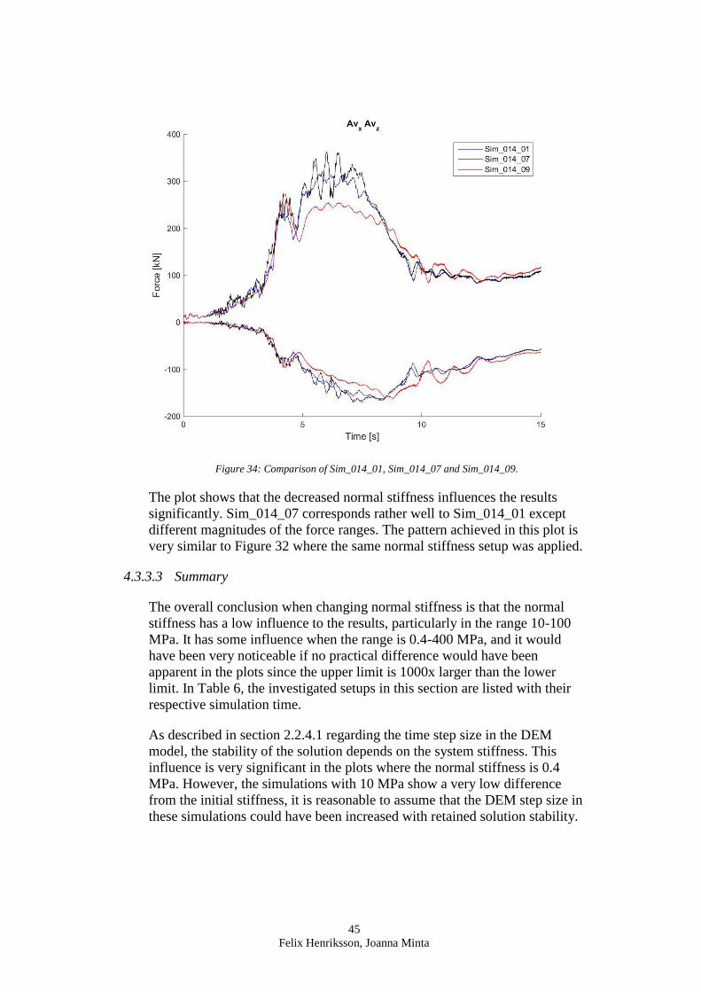
In Figure 34 Sim_014_01 (40 MPa), Sim_014_07 (400 MPa) and
Sim_014_09 (0.4 MPa) are compared. This is the same normal stiffness
setup as applied previously in Figure 32.
45
Felix Henriksson, Joanna Minta
Figure 34: Comparison of Sim_014_01, Sim_014_07 and Sim_014_09.
The plot shows that the decreased normal stiffness influences the results
significantly. Sim_014_07 corresponds rather well to Sim_014_01 except
different magnitudes of the force ranges. The pattern achieved in this plot is
very similar to Figure 32 where the same normal stiffness setup was applied.
4.3.3.3 Summary
The overall conclusion when changing normal stiffness is that the normal
stiffness has a low influence to the results, particularly in the range 10-100
MPa. It has some influence when the range is 0.4-400 MPa, and it would
have been very noticeable if no practical difference would have been
apparent in the plots since the upper limit is 1000x larger than the lower
limit. In Table 6, the investigated setups in this section are listed with their
respective simulation time.
As described in section 2.2.4.1 regarding the time step size in the DEM
model, the stability of the solution depends on the system stiffness. This
influence is very significant in the plots where the normal stiffness is 0.4
MPa. However, the simulations with 10 MPa show a very low difference
from the initial stiffness, it is reasonable to assume that the DEM step size in
these simulations could have been increased with retained solution stability.
46
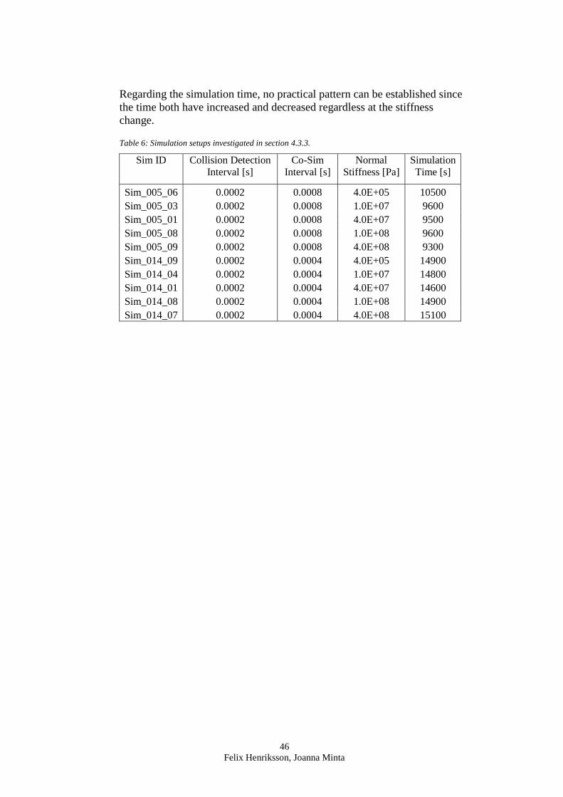
Felix Henriksson, Joanna Minta
Regarding the simulation time, no practical pattern can be established since
the time both have increased and decreased regardless at the stiffness
change.
Table 6: Simulation setups investigated in section 4.3.3.
Sim ID Collision Detection
Interval [s]
Co-Sim
Interval [s]
Normal
Stiffness [Pa]
Simulation
Time [s]
Sim_005_06 0.0002 0.0008 4.0E+05 10500
Sim_005_03 0.0002 0.0008 1.0E+07 9600
Sim_005_01 0.0002 0.0008 4.0E+07 9500
Sim_005_08 0.0002 0.0008 1.0E+08 9600
Sim_005_09 0.0002 0.0008 4.0E+08 9300
Sim_014_09 0.0002 0.0004 4.0E+05 14900
Sim_014_04 0.0002 0.0004 1.0E+07 14800
Sim_014_01 0.0002 0.0004 4.0E+07 14600
Sim_014_08 0.0002 0.0004 1.0E+08 14900
Sim_014_07 0.0002 0.0004 4.0E+08 15100

47
Felix Henriksson, Joanna Minta
5. Discussion
The authors consider the aim of this thesis, with respect to the limitations,
fulfilled. Nevertheless, it is always possible to identify things that could
have been investigated differently and some thoughts have arisen during the
work.
Something that could have been investigated more thoroughly is the
prescribed wheel loader motion. The propulsion shaft motion, that controls
rotation of the wheels, is manually created and is not stemming from
experimental measurements. If such measurement data would have been
available, a more realistic simulation could have been performed. However,
since a prescribed motion allows unlimited energy, which is unrealistic, a
force driven model would be necessary to bring the model closer to the
reality. This could be improved by inclusion of the powertrain and the
hydraulics in the Simulink model. As mentioned in the thesis these systems
exist, but to operate them require a driver model. If this could be
implemented, the assembled model could output information regarding fuel
consumption and performance, beside forces for design purposes.
Another aspect that could have been investigated is the material type that is
characterized in the DEM model. A change of material would also require
another type of bucket to match the material, since different buckets are used
for different applications. This could also lead to an investigation with a
completely different wheel loader model instead of the one used in this
thesis, L180G. This would of course require a lot of work, but the methods
are general and accordingly it would be possible to implement it for other
intended applications as well.
The selection of simulation setups is also a matter that could be discussed
since it is possible to set these parameters in practically any way. They were
set in accordance to the aim and are considered to have fulfilled the
requirements. Although, the setups could have been different e.g. the most
time consuming simulation was elapsing for about nine hours and it cannot
be assumed that an even longer simulation not would have led to more
accurate results. Such simulations were not performed due to a very low
difference between the nine-hour simulation and simulations with around
four-hour simulation time.

48
Felix Henriksson, Joanna Minta
6. Conclusions
From the results of this thesis it can be concluded, first of all, that the type of
simulation performed in this work could be a very useful tool to predict soil-
tool interaction forces, in this case a wheel loader bucket. This is supported
by comparison between measurements and simulation where it is clear that
the baseline, Sim_0_Initial, has a high correspondence with the
measurements. It can also be concluded that measurements are done with a
complex setup and the test data should be carefully studied before use. For
instance, there is a difference between the forces in the right and left A-pin
forces which probably stem from that the bucket did not enter the gravel pile
perpendicular during the test.
Generally, the results when comparing simulation to simulation show that a
decreased time interval for co-simulation and collision detection allows a
smoother and more stable solution. On the other hand, the decreased time
steps, increases the simulation time. The results with respect to normal
stiffness show that no significant and clear pattern can be extracted from the
results when the normal stiffness is kept between 10-100 MPa. When the
range is 0.4-400 MPa a more significant difference appears. As described in
section 4.3.3.3 a decreased normal stiffness means that a larger time step
size could be used without losing stability of the simulation. Since the
simulations with 10 MPa and 100 MPa shows very similar appearance, it
can be concluded that larger time step could be applied in the simulation
with retained stability.

49
Felix Henriksson, Joanna Minta
References
[1] "Nationalencyklopedin," [Online]. Available:
http://www.ne.se/uppslagsverk/encyklopedi/l%C3%A5ng/hjullastare.
[Accessed 11 02 2016].
[2] O. Kwangseok, K. Hakgu, K. Kyungeun, K. Panyoung and Y. Kyongsu,
"Integrated wheel loader simulation model for improving performance and
energy flow," Automation in Construction, vol. 58, pp. 129-143, 2015.
[3] M. Obermayr, Prediction of Load Data for Construction Equipment Using
the Discrete Element Method, Stuttgart: Shaker Verlag GmbH, Germany,
2013.
[4] "Adams - The Multibody Dynamics Simulation Solution," MSC Software
Corporation, [Online]. Available:
http://www.mscsoftware.com/product/adams. [Accessed 22 02 2016].
[5] S. Luding, "Introduction to Discrete Element Methods," European Journal
of Environmental and Civil Engineering, vol. 12, no. 7-8, pp. 785-826,
2008.
[6] E. Nezami, Y. Hashash, D. Zhao and J. Ghaboussi, "Simulation of front end
loader bucket-soil interaction using discrete element method," International
Journal for Numerical and Analytical Methods in Geomechanics, vol. 31,
pp. 1147-62, 2007.
[7] M. Marigo, "Discrete Element Method Modelling of Complex Granular
Motion in Mixing Vessels: Evaluation and Validation," University of
Birmingham, Birmingham, 2012.
[8] N. Bićanić, "Discrete Element Methods," in Encyclopedia of Computational
Mechanics, E. Stein, R. d. Borst and T. J. Hughes, Eds., Glasgow, John
Wiley & Sons, 2007.
[9] "Inpartik Simulation Software & Engineering," [Online]. Available:
http://www.inpartik.de/en/produkte.html. [Accessed 29 02 2016].
[10] "Simulation of soil-tool interaction," Fraunhofer ITWM, [Online].
Available: http://www.itwm.fraunhofer.de/en/departments/mdf/simulation-
of-soil-tool-interaction.html. [Accessed 23 02 2016].
[11] "Simulink," MathWorks, [Online]. Available:
http://www.mathworks.com/products/simulink/. [Accessed 22 02 2016].
[12] D. G. Price, Engineering Geology - Principles and Practice, Berlin:
Springer-Verlag Berlin Heidelberg, 2009.
[13] M. Budhu, Soil Mechanics and Foundations, 3 ed., John Wiley & Sons,
2011.
[14] M. Obermayr, C. Vrettos, P. Eberhard and T. Däuwel, "A discrete element
model and its experimental validation for the prediction of draft forces in
cohesive soil," Journal of Terramechanics, vol. 53, pp. 93-104, 2014.
[15] J. F. Labuz and A. Zang, "Mohr–Coulomb Failure Criterion," Rock
Mechanics and Rock Engineering, vol. 45, no. 6, pp. 975-979, 2012.

50
Felix Henriksson, Joanna Minta
[16] X. W. Guangcheng Yang, "Discrete Element Modeling for Granular
Materials," Electronic Journal of Geotechnical Engineering, vol. 17, 2012.
[17] "An Introduction to Discrete Element Method: A Meso-scale Mechanism
Analysis of Granular Flow," Journal of Dispersion Science and Technology,
vol. 36, no. 10, pp. 1370-1377, 2015.
[18] H. Takahashi, M. Hasegawa and E. Nakano, "Analysis on the resistive
forces acting on the bucket of a Load-Haul-Dump machine and a wheel
loader in the scooping task," Advanced Robotics, vol. 13, no. 2, pp. 97-114,
1999.
[19] C. Coetzee and D. Els, "The numerical modelling of excavator bucket filling
using DEM," Journal of Terramechanics, vol. 46, no. 5, pp. 217-227, 2009.
[20] C. Coetzee and D. Els, "Calibration of granular material parameters for
DEM modelling and numerical verification by blade–granular material
interaction," Journal of Terramechanics, vol. 46, pp. 15-26, 2009.
[21] H. Kuo, "Numerical and experimental studies in the mixing of particulate
material," The University of Birmingham, UK, 2001.
[22] C. Ergenzinger, R. Seifried and P. Eberhard, "A discrete element model to
describe failure of strong rock in uniaxial compression," Granular Matter,
vol. 13, pp. 341-364, 2011.
[23] F. V. Donzé, V. Richefeu and S. Magnier, "Advances in Discrete Element
Method Applied to Soil, Rock and Concrete Mechanics," Electronic Journal
of Geotechnical Engineering, vol. 44, p. 31, 2009.
[24] A. A. Shabana, Dynamics of multibody systems, 3 ed., New York:
Cambridge University Press, 2005.
[25] "Multibody Dynamics," MSC Software, [Online]. Available:
http://www.mscsoftware.com/application/multibody-dynamics. [Accessed
03 03 2016].
[26] "ParaView," Kitware Inc., [Online]. Available: http://www.paraview.org/.
[Accessed 11 04 2016].
[27] T. Ekevid, Coupling DEM Particles to MBS Wheel loader via Co-
simulation, Virtual Product Development, Volvo Construction Equipment,
2016.
[28] G. Söderlind and L. Wang, "Adaptive Time-Stepping and Computational
Stability," Journal of Computational Methods in Sciences and Engineering,
vol. 2, no. 3, pp. 1472-7978, 2003.

51
Felix Henriksson, Joanna Minta
Appendixes
Appendix 1: Complete list of simulation setups
Appendix 2: Plots of J pinhole forces

Appendix 1: Page 1
Felix Henriksson, Joanna Minta
APPENDIX 1: Complete list of simulation setups
Table 7: Complete list of test setups.
Sim ID Collision Detection
Interval [s]
Co-Sim
Interval [s]
Normal
Stiffness [MPa]
Simulation
Time [s]
Sim_0_Initial 0.0005 0.002 4.0E+07 4800
Sim_001_01 0.0001 0.0005 4.0E+07 16500
Sim_001_02 0.0001 0.0005 5.0E+07 17000
Sim_001_03 0.0001 0.0005 3.0E+07 17000
Sim_001_04 0.0001 0.0005 7.0E+07 16900
Sim_001_05 0.0001 0.0005 4.0E+05 17300
Sim_001_06 0.0001 0.0005 4.0E+08 16800
Sim_001_07 0.0001 0.0005 4.0E+06 17000
Sim_002 0.0005 0.001 4.0E+07 6700
Sim_003 0.0004 0.0008 4.0E+07 6900
Sim_004 0.0004 0.002 4.0E+07 5100
Sim_005_01 0.0002 0.0008 4.0E+07 9500
Sim_005_02 0.0002 0.0008 3.0E+07 9500
Sim_005_03 0.0002 0.0008 1.0E+07 9600
Sim_005_04 0.0002 0.0008 2.0E+07 9400
Sim_005_05 0.0002 0.0008 5.0E+07 9700
Sim_005_06 0.0002 0.0008 4.0E+05 10500
Sim_005_07 0.0002 0.0008 1.0E+09 10500
Sim_005_08 0.0002 0.0008 1.0E+08 9600
Sim_005_09 0.0002 0.0008 4.0E+08 9300
Sim_006 0.0002 0.002 4.0E+07 6900
Sim_007 0.0001 0.0006 4.0E+07 15500
Sim_008 0.0002 0.001 4.0E+07 8600
Sim_009 0.0001 0.001 4.0E+07 12600
Sim_010 0.0001 0.002 4.0E+07 10700
Sim_011 0.0002 0.0006 4.0E+07 11400
Sim_012 0.0003 0.0006 4.0E+07 10100
Sim_013 0.0001 0.0004 4.0E+07 19000
Sim_014_01 0.0002 0.0004 4.0E+07 14600
Sim_014_02 0.0002 0.0004 2.0E+07 15000
Sim_014_03 0.0002 0.0004 6.0E+07 14600
Sim_014_04 0.0002 0.0004 1.0E+07 14800
Sim_014_05 0.0002 0.0004 3.0E+07 14500
Sim_014_06 0.0002 0.0004 4.0E+06 15100
Sim_014_07 0.0002 0.0004 4.0E+08 15100
Sim_014_08 0.0002 0.0004 1.0E+08 14900
Sim_014_09 0.0002 0.0004 4.0E+05 14900

Appendix 1: Page 2
Felix Henriksson, Joanna Minta
Sim_015 0.0001 0.0002 4.0E+07 30100
Sim_016 0.0005 0.0005 4.0E+07 10200

Appendix 2: Page 1
Felix Henriksson, Joanna Minta
APPENDIX 2: Plots of J pinhole forces
Figure 35: Comparison of Sim_002 and Sim_016.

Appendix 2: Page 2
Felix Henriksson, Joanna Minta
Figure 36: Comparison of Sim_005_01, Sim_006, Sim_008 and Sim_014_01.
Figure 37: Comparison of Sim_007, Sim_009 and Sim_010.

Appendix 2: Page 3
Felix Henriksson, Joanna Minta
Figure 38: Comparison of Sim_001_01, Sim_013 and Sim_015.
Figure 39: Comparison of Sim_004, Sim_006 and Sim_010.

Appendix 2: Page 4
Felix Henriksson, Joanna Minta
Figure 40: Comparison of Sim_007, Sim_011 and Sim_012.
Figure 41: Comparison of Sim_013 and Sim_014_01.

Appendix 2: Page 5
Felix Henriksson, Joanna Minta
Figure 42: Comparison if Sim_005_01, Sim_005_03 and Sim_005_08.
Figure 43: Comparison of Sim_005_01, Sim_005_06 and Sim_005_09.

Appendix 2: Page 6
Felix Henriksson, Joanna Minta
Figure 44: Simulation Sim_014_01 compared with Sim_014_04 and Sim_014_08.
Figure 45: Comparison of Sim_014_01, Sim_014_07 and Sim_014_09.


Faculty of Technology 351 95 Växjö, Sweden Telephone: +46 772-28 80 00, fax +46 470-832 17