1

BUILDING CONNECTIONS: POLITICAL CORRUPTION AND ROAD

CONSTRUCTION IN INDIA

Jonathan Lehne† Jacob N. Shapiro‡ Oliver Vanden Eynde§

14 July 2017

Abstract

Politically-driven corruption is a pervasive challenge for development, but evidence of its

welfare effects are scarce. Using data from a major rural road construction programme in

India we document political influence in a setting where politicians have no official role in

contracting decisions. Exploiting close elections to identify the causal effect of coming to

power, we show that the share of contractors whose name matches that of the winning

politician increases by 83% (from 4% to 7%) in the term after a close election compared to

the term before. Regression discontinuity estimates at the road level show that political

interference raises the cost of road construction and increases the likelihood that roads go

missing.

Keywords: corruption; political connections; public procurement; kinship networks

JEL Codes: D72, D73, L14, O18

† Corresponding author; Paris School of Economics; Boulevard Jourdan 48, 75014 Paris, France; jonathan.lehne@gmail.com. ‡Princeton University, Woodrow Wilson School of Public and International Affairs; Robertson Hall, 20 Prospect Ave, Princeton, NJ 08540, USA; jns@princeton.edu. §Paris School of Economics; Boulevard Jourdan 48, 75014 Paris, France; olivervandeneynde@gmail.com.

2

1. INTRODUCTION

A growing literature documents the private returns to holding public office and the benefits from

political connections in both the developed and developing world (e.g. Fisman et al. 2014;

Cingano and Pinotti, 2013).1 It is often not clear from existing work to what extent the observed

gains by public officials or connected firms represent a welfare loss. We document political

influence over the allocation of individual road contracts in India’s major rural road development

scheme, providing econometric evidence that politicians intervene in the allocation of contracts

on behalf of members of their own network. By studying the performance of firms on contracts

that are likely to have been allocated preferentially, our paper provides direct evidence on the

welfare costs of political corruption. A distinguishing feature of our findings is that we study a

programme in which politicians have no formal role.

Specifically, we use data on more than 88,000 rural roads built under the Pradhan Mantri

Gram Sadak Yojana (PMGSY) programme to study how close-election victories shift spending.

Using regression discontinuity (RD) estimates to identify the causal effect of coming to power

we show in our preferred specification that the share of contractors whose name matches that of

the winning politician increases from 4% to 7% (an 83% increase). The magnitude of these

distortions are large relative to programme size. Applying our RD estimate to the full sample (i.e.

extrapolating from a LATE) would imply that state-level parliamentarians (MLAs) intervened in

the allocation of roughly 1,900 of the 4,127 road contracts let to connected contractors,

approximately $540M of the $1.2B spent on such roads and approximately 4% of the total spent

on the programme. These results are broadly representative of Indian polities. Our sample

consists of 4,058 electoral terms from 2001 to 2013, covering 2,632 constituencies in 24 of the

28 states which existed in our sample period.

The allocation of contracts to those with political connections does not conclusively prove

that politicians’ motives are corrupt. In an environment of imperfect information, MLAs could,

in theory, be better informed about, and better able to monitor, contractors in their own network,

and might therefore improve programme performance through benevolent interference. RD

estimation at the road level provides no evidence that is the case for PMGSY road construction.

1See Eggers and Hainmueller (2009) for members of the UK House of Commons and Truex (2014) for Chinese deputies.

3

Instead, we document direct negative welfare consequences for the people the programme is

supposed to serve.

We find that roads allocated to politically connected contractors are significantly more likely

never to be constructed. Census data at the village-level, collected after road construction was

officially completed, reveal that a number of roads listed as having been completed in the

PMGSY monitoring data, and for which payments were made, do not appear to exist. We define

a road as “missing” if a village it was meant to reach subsequently lacked “all-weather road

access” (PMGSY’s stated objective). The preferential allocation of roads is estimated to increase

the likelihood of a missing all-weather road by 86%. Assuming an extrapolation from a LATE

were valid, this would imply that an additional 497 all-weather roads are missing as a result of

corrupt political intervention and, that the 857,000 people these roads would have served, remain

at least partially cut-off from the wider Indian economy. Political interference in PMGSY is also

detrimental when road construction actually takes place. Further road-level RD estimations show

that roads allocated to connected contractors are more expensive to construct. These results

indicate that corruption in PMGSY imposes social costs while providing no offsetting benefits in

terms of efficiency or quality. Importantly, because road locations were largely determined

before the elections we study, the impact of the corruption examined here arises primarily

from who is allocated a contract rather than where a road is built.

Our paper’s first contribution is to provide micro-evidence on informal channels of political

influence. A growing number of papers document how firms benefits from political connections,

(Amore and Bennedsen, 2013; Do et al., 2015). Khwaja and Mian (2005) show that banks in

Pakistan lend more to politically connected firms - in spite of higher default rates. Cingano and

Pinotti (2013) show that connected firms in Italy benefit from a misallocation of public

expenditures, which helps them to increase profits. Mironov and Zhuravskaya (2016) show that

Russian firms who funnel money in the run-up to elections are significantly more likely to

receive procurement contracts after the election. We add to these recent contributions, by

showing a link between the election of Indian legislators and the allocation of PMGSY road

contracts to connected contractors. Preferential allocation in the context of PMGSY is

particularly striking, because state-level legislators do not have any formal role in the allocation

of contracts. In fact, this programme’s bidding rules were designed in ways that should have

forestalled political influence at the bidding stage (NRRDA 2015). Our evidence on preferential

4

allocation in such a programme helps us to understand the economic role of local politicians, in

particular in India. Recent work shows how Indian state legislators have a sizable impact on local

economic outcomes. Asher and Novosad (2017) show that employment is higher in

constituencies whose MLAs are aligned with the state-level government. Prakash et al. (2015)

find that the election of criminal MLAs leads to lower economic growth in their constituencies.

Fisman et al. (2014) show that the assets of marginally elected MLAs grow more than those of

runners-up, which confirms the idea that there are substantial private returns to holding office.2

Existing work has shown that MLAs have influence over the assignment of bureaucrats (Iyer and

Mani, 2012). In further analysis, our paper documents that the misallocation of roads is stronger

when MLAs and local bureaucrats (District Collectors) share the same name, and weaker when

local bureaucrats are up for promotion and subject to greater scrutiny. These results suggest that

bureaucrats play an important role in facilitating political corruption, and they help to explain

how politicians can exert influence even when they do not have any formal role. Hence, our

paper provides micro-evidence that accounts for MLAs’ disproportionate impact on the

economies of their constituencies, and for the private benefits they derive from holding office.

Our second contribution is to demonstrate a new approach to quantifying politicians’

influence over public procurement contracting. The core challenges we confront in doing so are

that: (i) there is no information on actual connections between politicians and the contractors

active in their constituency; and (ii), to the extent that politicians intervene in the allocation of

roads on contractors’ behalf, such improper interference would not be documented. We address

the first problem by constructing a surname-based measure of proximity between candidates for

state-level legislatures and contractors. This approach follows a number of papers that use Indian

surnames as identifiers of caste or religion (e.g. Hoff and Pandey 2004, Field et al. 2008,

Banerjee et al. 2014). Dealing with the second issue – identifying improper intervention –

requires isolating the variation in proximity to contractors that results from the MLA coming to

power. We do so with a regression discontinuity approach that exploits the fact that in close

elections, candidates who barely lost are likely to have similar characteristics to those who were

barely elected. If MLAs are intervening in the assignment of contracts, one would expect a shift

in the allocation towards contractors who share their name, and no equivalent shift for their 2 Gulzar and Pasquale (2016) also confirm the importance of MLAs for local development outcomes. In blocks that are split between different MLAs, the implementation of India’s rural employment guarantee is worse than in blocks that are entirely part of one MLAs constituency.

5

unsuccessful opponents. This approach to detect undue influence is what Banerjee et al. (2013)

refer to as a “cross-checking” method for identifying corruption: the comparison between (i) an

actually observed outcome, and (ii) a counterfactual measure which should be equivalent to the

former in the absence of corruption.3 In our setting, if politicians are not intervening in the

allocation of road projects, they should be no ‘closer’ to contractors than their unsuccessful

opponents.

Our third contribution is to shed light on the social costs of political connections. In principle,

allocating contracts to connected firms could be beneficial – politicians could use private

information to select higher quality firms, or they could use their social networks to discipline

contractors. And while the common intuition is that political influence has deleterious effects,

few papers document the social costs of political connections. For example, Mironov and

Zhuravskaya (2016) show that politically connected firms have lower average productivity.4 Our

unusually rich data allows us to examine the performance of contractors in the exact contracts

that are likely to be preferentially allocated. We introduce a particularly powerful measure of

contractor underperformance: “missing roads”. These are roads that are complete in the PMGSY

records and for which payments have been made, but that do not appear in the (independently

conducted) Population Census. This approach allows us to provide very clear evidence of the

welfare costs of undue political influence: the roads that are built by connected contractors are

more likely to go missing.

This finding speaks to an old debate in the corruption literature: the contrast between costly

rent-seeking or “greasing the wheels”. Theoretically, corruption is typically thought of as rent-

seeking. Public officials use their control over the allocation of contracts or the provision of

services to ask for bribes (e.g. Becker and Stigler, 1974; Krueger, 1974; Rose-Ackerman, 1975;

Shleifer and Vishny, 1993). This behaviour is most likely to arise in contexts where enforcement

3Other exponents of the “cross-checking” approach include Acemoglu et al. (2014), Golden and Picci (2005), Reinnika and Svensson (2004), Olken (2007), Fisman (2001), and Banerjee et al. (2014a). Several countries conduct regular audits of local government expenditure and make the results publicly available. Examples of research based on these data include: Ferraz and Finnan (2008 and 2011) and Melo et al. (2009) for Brazil; or Larreguy, Marshall and Snyder Jr (2014) for Mexico; and Bobonis et al. (2016) for Puerto Rico. In some settings, corruption can be observed directly, as in the driving license experiment conducted by Bertrand et al. (2007) or in the trucking survey of Olken and Barron (2009). 4Cingano and Pinotti (2013) measure the welfare costs of preferential contract allocation through simulation techniques. Fisman and Wang (2015) show that politically connected firms in China have higher worker death rates.

6

is weak and officials are poorly remunerated.5 The so-called “greasing the wheels” hypothesis

argues that such corruption can be optimal in a second-best world, by allowing agents to

circumvent inefficient institutions and regulation (Huntington 1968, Lui 1985). In principle, both

arguments could apply to the preferential assignment of PMGSY roads by Indian MLAs.6

However, the evidence we present on missing roads clearly supports the rent-seeking hypothesis,

which is consistent with most of the recent work that relies on the direct observation of

corruption (e.g. Bertrand et al., 2007) or cross-checking approaches (Banerjee et al., 2013). The

simple “missing infrastructure” measure we propose, can be used in a wide variety of contexts. It

is a particularly cost-effective alternative to physical road audits as conducted by Olken (2007).

Improvements in remote sensing techniques mean that confirming the existence of

administratively completed projects will become a very economical way to detect and measure

the diversion of public funds, even when census data is not available.

Our fourth contribution is to shed new light on the electoral motives for corruption. A

standard explanation for why politicians target patronage along in-group lines, which in India

often means caste, is that it acts as a form of vote-buying (Banerjee et al., 2014). Targeting

patronage could be easier within ethnic or caste groups (Chandra 2004, Horowitz 1985). In the

context of large-scale contracts like the ones we study, patronage could also be used to reward

firms who help fund political campaigns. Mironov and Zhuravskaya (2016) document how

Russian politicians allocate contracts to firms who funded their election. Sukhtankar (2012)

shows that political candidates in India siphon funds from sugar mills in election years.

However, in our analysis, we find no evidence that the preferential allocation of roads or cost

inflation increase immediately before or after election dates. If vote-buying is going on for this

programme it must be a long-run transaction. If anything, we observe that roads built by

connected contractors are less expensive around election periods – which could be consistent

with higher scrutiny in election times. In the context of Puerto Rican municipalities, Bobonis et

al. (2016) show that financial audits are most effective in reducing corruption when they are

conducted shortly before elections. A recent paper by Bohlken (2016) argues that road

5 In the case of Indian MLAs, calculating efficiency wages (as suggested by Becker and Stigler, 1974) may be complicated by the fact that candidates frequently need to pay their parties significant sums for their place on the ticket. This could prompt them to engage in corrupt behaviour once elected (Jensenius, 2013). 6 An intermediate argument is that initial corrupt allocations may not matter if there is scope for Coasian bargaining. Sukhtankar (2015) finds evidence in this direction for the allocation of the wireless spectrum in India.

7

completion in PMGSY is higher when the ruling party in the state is aligned with local MLAs in

marginal constituencies, which suggests that voters hold the state government accountable for

PMGSY performance. As a second test of electoral motives for corruption, we exploit India’s

2008 re-drawing of electoral constituency boundaries to study the behaviour of MLAs in regions

that have become “politically irrelevant” after the redistricting. We find no evidence of different

behaviour in these regions. Thus, while our paper documents the preferential allocation of road

contracts, we find no evidence linking corrupt behaviour to electoral incentives.

Our results are more consistent with either standard in-group favouritism, or a subtler

mechanism by which caste or kinship networks facilitate corrupt exchange under the threat of

punishment. Corruption is illegal and therefore requires either trust among collaborators, or a

predictable ability to sanction defections, both of which are more likely to exist between

members of the same family, ethnic group, or network (Lambsdorff 2002; Tonoyan 2003). While

we are unable to test it explicitly, this interpretation fits our findings and the context of PMGSY.

The involvement of the central government in the programme guarantees a minimum level of

monitoring. In line with the idea that contractors trade off rent-seeking and the cost of detection,

we find no evidence that preferential allocation affects the performance markers that are most

easily observed in the administrative data collected at the central level: over-runs and delays. We

also find that preferentially allocated contracts are less expensive in the run-up to elections, a

time when monitoring may be greater.

The remainder of the paper proceeds as follows. Section 2 provides context on PMGSY, the

role of MLAs, and Indian surnames as identifiers of caste or religion. Section 3 describes the

dataset used in the analysis. Section 4 outlines the empirical strategy. Section 5 presents the main

results on re-allocation and robustness. Section 6 analyses the social costs of re-allocation.

Section 7 provides evidence for the intermediary role of bureaucrats. Section 8 evaluates

electoral motives for corruption. Section 9 concludes.

2. BACKGROUND

2.1 PMGSY

8

In the year 2000, an estimated 330,000 Indian villages or habitations – out of a total of 825,000 –

were not connected to a road that provided all-weather access (NRRDA 2005). Their inhabitants

were at least partially cut-off from economic opportunities and public services (such as health

care and education). To address this lack of connectivity, the Indian government launched the

Pradhan Mantri Gram Sadak Yojana (PMGSY) in December 2000. Its goal was to ensure all-

weather access to all habitations with populations over 1,000 by the year 2003, and to those with

more than 500 inhabitants by 2007. In hill states, desert and tribal areas, as well as districts with

Naxalite insurgent activity, habitations with a population over 250 were targeted (NRRDA 2005).

The proposed network of roads was determined ex-ante in 2001, and the implementation of

PMGSY in subsequent decades has consisted of the gradual realisation of this “Core Network”.

The programme has been described as “unprecedented in its scale and scope” (Aggarwal

2017), with roadwork for over 125,000 habitations completed and another 22,000 under

construction as of November 2016.7 A second phase of the scheme (PMGSY II), launched in

2013, targets all habitations with populations over 100. According to World Bank estimates,

expenditures under PMGSY had reached 14.6 billion USD by the end of 2010, with a further 40

billion USD required for its completion by 2020 (World Bank, 2014).

Several studies have focused on the first-order research question that arises in relation to

PMGSY: its impact on habitations and the lives of their inhabitants. Asher and Novosad (2016)

analyse the employment effects of the programme in previously unconnected villages. They find

that a new paved road raises participation in the wage labour market with a commensurate

decrease in the share of workers employed in agriculture. This translates into higher household

earnings and a rise in the share of households who live in houses with solid roof and walls.

Aggarwal (2017) also finds a positive effect on employment and reduced price dispersion among

villages. While these studies analyse what PMGSY has achieved, this paper looks at how it has

been implemented.

Compared to other public works programmes, the implementation of PMGSY stands out

because of its reliance on private contractors combined with relatively strong monitoring and

quality assurance provisions, designed to limit the scope for undue corruption. All tenders have

to follow a competitive bidding procedure, for which the rules were prescribed by the National 7 OMMAS (Online Management, Monitoring and Accounting System), http://omms.nic.in/, accessed in November 2016.

9

Rural Roads Development Agency (NRRDA) and set out in the so-called Standard Bidding

Document (SBD). The SBD consists of a two envelope tendering process administered at the

circle level. Each bid consists of both technical and financial volumes. The technical bids are

opened first. Contractors have to fulfil eligibility criteria, taking into account factors such as their

current workload and experience. Only the financial bids of contractors whose technical bids are

found to meet the requirements are evaluated, and subject to meeting the technical standards, the

lowest bidder has to be selected. After the contract has been assigned, administrative data on the

programme is gathered, while central and state-level inspectors can carry out quality inspections.

In spite of these provisions, there remains clear scope for corruption, and the financial incentives

are sizeable given the scale of the project.8 A large number of newspaper reports document

alleged corruption in PMGSY.9 Corruption in PMGSY could take several forms, and the possible

manipulation of road allocations is one of the challenges for impact evaluations of the

programme (Asher and Novosad, 2016).10 Our paper tests for a specific form of corruption:

interventions by state-level parliamentarians (MLAs) in the allocation of road contracts (but not

of the location of roads) within their constituencies.

An advantage of focussing on MLAs in this context is that under the programme guidelines,

they should be in no way involved in the tendering process or the selection of contractors. In fact,

they are granted practically no official role in the implementation of PMGSY whatsoever.11

Funding for PMGSY comes primarily from the central government. The scheme is managed by

local Programme Implementation Units (PIUs), which are under the control of State Rural Roads 8Existing work reports that the price bid of only one firm was evaluated in 95% of a random sample of 190 road contracts issued between 2001 and 2006 in Uttar Pradesh; i.e. only one bid submitted or all other bids were disqualified based on technical requirements (Lewis-Faupel et al., 2016). 9 Examples include articles in “The Hindu” on April 11 2012, “The Economic Times” on March 8 2013, “The Arunachal Times” on March 6 2013, the online news-platform “oneindia” on July 31 2006, and “Zee News” on 30 August 2014. For example, the “oneindia” article reports that the former Chief Minister of Sikkim accused the current administration of “widescale corruption” in the implementation of PMGSY and “alleged that the works were awarded to relatives of Chief Minister, Ministers and MLAs of the state”. 10 These authors find that the habitation population figures reported to PMGSY had been manipulated, particularly around the 1,000 and 500 population cut-offs used to target the programme. 11 MLAs are mentioned in the PMGSY guidelines, but only in reference to the initial planning stage. Intermediate panchayats and District panchayats were responsible for drawing up a planned “Core Network” which encompasses all future roadwork to be carried out under PMGSY. These plans were to be circulated to MPs and MLAs, whose suggestions were to be incorporated. MLAs could therefore have influenced which habitations were targeted ex-ante through official channels. However, this role is irrelevant for the timing of the construction work and assignment of road contracts, on which MLAs have no formal influence. Moreover, these consultations took place prior to our sample period. The majority of MLAs in our sample were not in office at the time and therefore had no opportunity to review the planned network. Our results are unchanged when we drop MLAs who were in office prior to 2001 from the sample (see Appendix Table A10).

10

Development Agencies (SRRDA). These agencies are responsible for inviting tenders and

awarding contracts. Given their lack of formal involvement, any systematic relationship between

MLAs and the contractors working in their constituencies can therefore, in itself, be construed as

evidence for an irregularity in the allocation of contracts.

2.2 The role of MLAs

MLAs, or Members of Legislative Assembly, are India’s state-level parliamentarians. They are

elected for 5-year terms in a first-past-the-post voting system in state-wide elections. In general,

the state assembly elections in India’s different states do not coincide. MLAs are typically

nominated by the party, and each MLA represents a single constituency.

Is it plausible that these MLAs would seek to intervene on behalf of specific contractors? While

their official function is to represent their constituents in state legislative assemblies, surveyed

MLAs overwhelmingly report this to be a minor part of their work (Chopra 1996). State

assemblies meet rarely and according to Jensenius (2013), individual legislators have little

impact on political decisions: “much more important to the MLAs are all their unofficial tasks of

delivering pork, blessing occasions, and helping people out with their individual problems”.

Qualitative accounts suggest that MLAs spend much of their time receiving requests from their

constituents. Describing such meetings Chopra (1996) writes “constituents came to ask for

favours that clearly contravened rules and laws”. MLAs often respond to requests by passing

them on to ministers or high-ranking officials, and they are also known to put pressure on

bureaucrats by threatening them with reassignment (Iyer and Mani 2012, Bussell 2015).

2.3 Surnames as a measure of interpersonal proximity in India

To measure proximity between MLAs and contractors we construct a proxy based on politicians’

and contractors’ surnames.12 Indian surnames can be an indicator of caste affiliation, religion, or

geographic provenance. Naming conventions differ across India; it is common for Indians to

have multiple surnames and the same name can appear in different positions within the list of

names. This is also true of caste identifiers. Still, as a general rule, the last name will be caste or

religion specific and follow the paternal line. This pattern is sufficiently strong for Indian

12 Angelucci et al. (2010), and Mastrobuoni and Patacchini (2012) also use name-based matching to study social networks.

11

surnames to have been used as identifiers of caste or religion in many empirical studies

(Banerjee et al. 2014, Hoff and Pandey 2004, Vissa 2011, Fisman et al. 2017, Field et al. 2008).

One clear exception to this rule is Tamil Nadu, where surnames do not exist, and we will

document that our method does not work for Tamil Nadu. Surnames are a significantly more

accurate predictor of connections when comparing individuals from the same area or linguistic

region. The contractors and politicians in our setting are highly likely to be from the same state

and will in many cases be from the same district or constituency.

Our paper treats a match between the names of a politician and a contractor as a rough

overall measure of proximity, without seeking to establish whether the individuals are of the

same religion, caste, or (potentially) family. All of these types of connections are likely to

increase the probability that a contractor would approach an MLA when bidding for a contract,

and that the MLA would be receptive.

Name-based matching is an imperfect measure of proximity. Contractors may have

connections to politicians without sharing a name, or equally, share a name but have no

connection. Surnames that are not caste-identifiers, former honorific titles for example, are likely

to dilute the accuracy of the measure. Hence, the estimates in this paper can be viewed as a lower

bound for MLAs’ true effect on contract allocation.

3. DATA

The empirical strategy requires three kinds of data. Information on contractors and agreements is

available in the administrative records of the PMGSY project, at the road level. Data on political

candidates and elections are at the level of the assembly constituency. These two are linked using

the population census, which allows for habitations to be matched to constituencies, as well as

providing additional covariates used in the analysis.

3.1 PMGSY data

The administrative records of projects sanctioned under PMGSY are publicly available in the

Online Management, Monitoring, and Accounting System (OMMAS). The dataset used for this

paper contains the agreement details of 110,185 roads serving 188,394 habitations. This

12

information includes: the date of contract signing, sanctioned cost, proposed length, proposed

date of completion, name of the contracting company, and – crucially for this analysis – the

name of the winning contractor. In addition to the agreement details, which precede road

construction, the OMMAS also contains later data on the physical progress of work, data on

completed roads, and reports from subsequent quality inspections. These are used in section 6 to

evaluate the effect of political interference on the efficiency and quality of road construction.

3.2. Assembly election data

The Election Commission of India (ECI) publishes statistical reports on assembly elections that

record each candidate’s name, party, gender and vote share. Since 2003, candidates have

moreover been required to submit sworn affidavits to the ECI with information on their assets,

liabilities, educational attainment, and any pending criminal cases. Both the election reports and

affidavits are publicly available from the ECI in pdf format. This paper draws on digitised

versions of this information from four separate sources. Table A1 of the online appendix lists

these sources – which cover different time periods and variables – and describes which variables

from each source are used in the analysis (all these secondary sources are based on the ECI).13

Assembly elections operate on a plurality rule. While the median number of candidates per

election is eight, typically only the top-2 candidates are competitive: the third placed candidates

average 7% of the vote, the fourth placed candidates average 3%, the fifth 1.6% and the rest less

than 1%. To estimate the RD we restrict attention to elections in which there are PMGSY

contracts issued in the term before and after the election and focus on the winner and runner-up.

This gives us a sample of 8,116 candidates in 4,058 elections from 2001 to 2013, covering 2,632

constituencies. In our preferred specification we estimate on the resulting sample of 8,116

candidate-terms. In a placebo test we show that the effects are not present for the contrast

between the runner-up and third-placed candidate. Map 1 (of the online appendix) shows the

constituencies included in the sample which cover 24 of the 28 states that existed during the

13 The matching process is complicated by discrepancies in the spelling of constituency and candidate names. These occur not only across datasets but also across time within datasets. Using different secondary sources helps us to construct a consistent data set. In a small number of cases, multiple constituencies within the same state have the same name. We drop all of these constituencies from our sample, to prevent false matches between election datasets and to avoid the risk of assigning roads to the wrong constituency.

13

timeframe under analysis.14 Map 2 shows the constituencies which had at least one close election,

the sub-sample for our local linear RD estimation.

3.3. Matching roads and electoral terms using census data

The Population Census of India 2001 contains village-level data on demographic and socio-

economic variables used as controls in the analysis. We use the Village Amenities part of the

2011 census, to identify the ‘missing roads’ evaluated in section 6.

The 2001 census is also the source for habitation-level data, which was collected by the

PMGSY in order to determine the prioritisation of roads. This includes information on the size of

the population (the project guidelines stipulate that habitations above certain population

thresholds are to be prioritised), whether or not it was connected to a road in 2001, and if so,

whether this road provided all-weather access. Moreover, it reports the MLA constituency in

which it each habitation was situated in 2001.

Using this information, it is possible to match PMGSY roads (at the habitation-level) to the

assembly election data described in the previous sub-section. However, changes in the

delimitation of MLA constituencies – which took effect in mid-2008 – led to changes in

boundaries, the abolition of some constituencies, and the creation of new ones. For roads built in

electoral terms after the new delimitation we use the coordinates of habitations and match these

to GIS data on constituency boundaries.

While the census data allows for spatial matching of roads and constituencies, it is also

necessary to match them in time. Road contracts are allocated to electoral terms based on the

date of the agreement, as recorded in the PMGSY data. In order to precisely assign road

contracts, it is necessary to set an exact date that marks the end of one term and the beginning of

the next. We define this as the date on which the results of an election are announced.15

3.4 Matching politicians and contractors using surnames

In the electoral terms that preceded and followed the elections in the sample, 88,020 road

agreements were signed. For each political candidate, we assess whether they share a surname

with the contractors who received projects in their constituency in the term after the election. For 14 Goa, Meghalaya, Nagaland and Sikkim are not part of our sample. 15 These dates were collected from the website www.electionsinindia.com (accessed in 2015).

14

every politician-contractor pair, we exclude all names except for each individual’s final name

and then look for matches among these surnames. The results are, however, robust to broader

definitions of matches.16 To account for different spellings of the same name, we implement a

fuzzy matching algorithm optimised for Hindi names.

Matches are aggregated at the electoral term level as follows. The variable 𝑚𝑎𝑡𝑐ℎ!"#$ takes

the value of 1 if the contractor for a road agreement n, signed in constituency j in term t, shares a

name with candidate i, and 0 otherwise. This variable is determined for the N road agreements

signed in the constituency during an electoral term. 𝑠ℎ𝑎𝑟𝑒!"# is defined as the share of contracts

in term t allocated to contractors who share a candidate’s name. 𝑠ℎ𝑎𝑟𝑒!"#!! provides the

equivalent share for contracts in the term prior to the election in which a candidate took part.

𝑠ℎ𝑎𝑟𝑒!"# =𝑚𝑎𝑡𝑐ℎ!"#$!

!!!

𝑁!" 𝑠ℎ𝑎𝑟𝑒!"#!! =

𝑚𝑎𝑡𝑐ℎ!"#$!!!!!!

𝑁!"!!

The dependent variable in the main regressions is the difference between these two:

∆𝑠ℎ𝑎𝑟𝑒!"# = 𝑠ℎ𝑎𝑟𝑒!"# − 𝑠ℎ𝑎𝑟𝑒!"#!!,

which we calculate for all candidates 𝑖 ∈ {𝑤𝑖𝑛𝑛𝑒𝑟, 𝑟𝑢𝑛𝑛𝑒𝑟-𝑢𝑝}.

A complication arises in elections where winning and losing candidates have the same

surname. It is not possible to estimate the effect of winning an election in this situation, as

candidates who lost will see their proximity to contractors evolve in parallel to that of the elected

politicians. In the main regressions, we therefore exclude candidates from elections where this

issue arises.

3.5 Descriptive statistics

Table 1 reports descriptive statistics for the sample of candidates used in the main regressions.

For the average term in the sample, the number of road contracts signed is 28. The average value

of 𝑠ℎ𝑎𝑟𝑒!"#!! – which can be construed as a baseline measure of the frequency of surname-

matches – is 4%. There is however, significant geographic variation in the frequency of matches,

ranging from a mean of 0% in Mizoram to a mean of 13% in Andhra Pradesh (Map 3 of the

16 The results are robust to considering all matches among individuals’ names (excluding their first name) or only matches based only on the last two names.

15

online appendix shows this variation at the constituency-level).17 However, these means do not

distinguish between winning and losing candidates – the variation exploited in the empirical

strategy below.

17 It is likely that these baseline frequencies lead to heterogeneous treatment effects. In states or constituencies, where the distribution of names is such that matches are relatively rare, a politician who is elected may not have many potential contractors of the same name to allocate roads to.

16

Table 1A: Descriptive Statistics (Candidate/Constituency)

Variable Observations Mean Std. Dev. Min Max Panel A: Roads allocated to contractors of the same name Sharet-1 8116 0.037 0.141 0.000 1.000 Sharet 8116 0.035 0.134 0.000 1.000 ΔShare 8116 -0.002 0.151 -1.000 1.000 Panel B: Candidate characteristics Vote share 8036 0.279 0.103 0.020 0.837 Margin 8116 0.000 0.102 -0.695 0.695 Incumbent 8116 0.282 0.450 0.000 1.000 Runner-up previous election 8116 0.147 0.354 0.000 1.000 Age 7357 49.164 10.207 23 87 Female candidate 8116 0.062 0.242 0.000 1.000 Candidate with criminal charges 5990 0.196 0.397 0.000 1.000 Total assets (1000000s of INR) 5009 106 4740 0.000 300000 Liabilities (1000000s of INR) 5286 1.841 17.800 0.000 644 University graduate 5286 0.596 0.491 0.000 1.000 Postgraduate degree 5286 0.192 0.394 0.000 1.000 Congress candidate 8098 0.290 0.454 0.000 1.000 BJP candidate 8098 0.192 0.394 0.000 1.000 Named Kumar 8116 0.058 0.234 0.000 1.000 Named Lal 8116 0.022 0.145 0.000 1.000 Named Patel 8116 0.009 0.094 0.000 1.000 Named Ram 8116 0.018 0.133 0.000 1.000 Named Reddy 8116 0.016 0.124 0.000 1.000 Named Singh 8116 0.112 0.316 0.000 1.000 Named Yadav 8116 0.014 0.117 0.000 1.000 Panel C: Constituency characteristics Reserved seat 8116 0.275 0.446 0.000 1.000 Road countt 8116 27.691 30.822 1.000 479 Road countt-1 8116 22.086 25.744 1.000 388 Mean road lengtht 8116 5.833 3.999 0.350 42.654 Mean road lengtht-1 8116 4.963 3.838 0.410 53.985 Mean population 7822 961.697 633.986 30.000 7230 Mean SC/ST population 7822 244.078 193.401 0.000 2283 Mean connectivity 7822 0.561 0.308 0.000 1.000 Note: The number of observations varies due to missing values. Reserved seat refers to constituency reserved for MLAs from scheduled castes or tribes. Road countt is computed at the term-level by counting the number of road contracts signed in a constituency within a term. Mean road length is the average length of roads (in km) built in a constituency and term. Mean population and mean SC/ST population are averages of 2001 census data for all of a constituency’s villages. Mean connectivity is the share of a constituency’s villages that had all-weather road access at the time of the 2001 census.

17

Table 1B: Descriptive Statistics (Roads built by same name contractors)

Variable Observations Mean Std. Dev. Min Max Panel A: Road construction Length of road 4921 3.997 3.654 0.01 41 Bridge 4921 0.008 0.091 0 1

Cost (1000000s of INR) 4921 133.7 149.625 3 2730.56

Log of (sanctioned cost/km) 4921 3.347 0.651 0.0312 11.24

Days overrun 3202 588.0 543.8 -1750 3932

Actual cost/sanctioned cost 3867 0.954 0.257 0 9.35

Failed Inspection 1513 0.365 0.482 0 1

Missing all-weather road 1815 0.260 0.438 0 1

Missing any road 1815 0.025 0.156 0 1

Panel B: Local Geography Altitude 4921 588.707 805.450 0 4864.6 Ruggedness 4921 0.243 0.657 0 8.506

Forest Cover 4494 0.398 0.110 0 0.861

Distance to nearest town 4482 22.622 20.994 0 244

Panel C: Village Demographics Total population 4,464 2416.8 3425.2 1 49192 Number of households 4,464 449.2 707.8 1 9851 Village area 4,482 722.7 1772.0 0 67737 Sex ratio 4,462 1.062 0.101 0.583 2.1 Population under 6 4,464 0.179 0.042 0 0.335 SC share 4,464 0.173 0.154 0 1 ST share 4,464 0.106 0.238 0 1 Panel D: Village Socioeconomic Characteristics Literacy 2,952 54.019 16.546 0 100 Employment 2,952 39.166 12.141 12.938 100 Male employment 2952 0.499 0.075 0.227 1

Female employment 2,952 27.431 19.772 0 82.304 Drinking water 4,464 0.998 0.047 0 1 Power supply 4,461 0.767 0.423 0 1 Phone connections 4,482 10.576 79.597 0 1713 Road connectivity in 2001 4921 0.311 0.463 0 1 Note: Table 1b provides descriptive statistics for the sample used in Tables 4, 5 and columns 4-6 of Table 6. Cost, delays, cost overruns, and quality inspections are based on the PMGSY data. Quality is a dummy variable equal to one if the road is “unsatisfactory” or “in need of improvement” in latest inspection. “Missing roads” are defined on the basis of the 2011 census and the PMGSY data. The dummy for the all-weather road missing variable takes the value of one if any village on the route of an officially completed road lacks all-weather road access according to the 2011 census. For the missing-any-road definition, we set the missing dummy equal to one if all villages on the completed PMGSY road had no road of any type (tarmac, gravel, or water bound macadam) according to the 2011 census.

18

4. EMPIRICAL STRATEGY

A natural control group for elected politicians are those who aspire to the same office. If being an

MLA is associated with the power to intervene in the allocation of roads in one’s constituency,

one would expect the share of contractors with the same name as a winning candidate to be

higher than the corresponding share for losing candidates.

As our main outcome of interest, we use the first difference of 𝑠ℎ𝑎𝑟𝑒!"# . Taking the

difference should remove unobservable, time-invariant characteristics of an individual candidate

that may be correlated with the number of matches with contractors. In our context, this is

primarily a way of controlling for specificities that individual names may have within certain

constituencies. Some candidates’ names will be more common than others. Some may be more

prevalent among certain professions (e.g. contractors) for historical reasons. Under the

assumption that winning and losing candidates had a common trend in their share of matches

with contractors, a simple difference-in-differences (DiD) approach would be sufficient for

identification. However, given that winners are likely to be systematically different from losing

candidates in many respects, it is possible that they may face divergent trends in 𝑠ℎ𝑎𝑟𝑒!"# that are

not determined by election outcomes. This suggests the use of a regression discontinuity (RD)

design.18

In order to identify whether there is a causal relationship between the election of politicians

and the allocation of road contracts in their constituencies, we exploit the fact that in close

elections, the assignment of victory can be considered conditionally independent of subsequent

contracting patterns. The underlying assumption is that candidates who won an election by a

very small margin are comparable to those who narrowly lost (Lee, 2008). We evaluate whether

this assumption holds in our sample by running balance checks on observable characteristics (see

below). In order to determine how close elections were, we define the variable 𝑚𝑎𝑟𝑔𝑖𝑛!"# for

candidate i in constituency j and term t:

𝑚𝑎𝑟𝑔𝑖𝑛!"# =𝑣𝑜𝑡𝑒 𝑠ℎ𝑎𝑟𝑒(𝑤𝑖𝑛𝑛𝑒𝑟)!" − 𝑣𝑜𝑡𝑒 𝑠ℎ𝑎𝑟𝑒(𝑟𝑢𝑛𝑛𝑒𝑟𝑢𝑝)!" 𝑖𝑓 𝑤𝑖𝑛𝑛𝑒𝑟!"# = 1 𝑣𝑜𝑡𝑒 𝑠ℎ𝑎𝑟𝑒(𝑟𝑢𝑛𝑛𝑒𝑟𝑢𝑝)!" − 𝑣𝑜𝑡𝑒 𝑠ℎ𝑎𝑟𝑒(𝑤𝑖𝑛𝑛𝑒𝑟)!" 𝑖𝑓 𝑤𝑖𝑛𝑛𝑒𝑟!"# = 0

18We obtain similar results when estimating the RD using levels with 𝑠ℎ𝑎𝑟𝑒!"# as the dependent variable (Table A2). Taking the first difference of𝑠ℎ𝑎𝑟𝑒!"# in our RD estimation contributes to precision and allows for a direct comparison of our RD results with the DiD results for the full sample (see discussion of LATE in section 5).

19

We estimate equation (1) in a non-parametric RD for a range of bandwidths 𝜇, controlling for

the assignment variable 𝑚𝑎𝑟𝑔𝑖𝑛!"# and its interaction with 𝑤𝑖𝑛𝑛𝑒𝑟!"# to allow for a different

relationship between ∆𝑠ℎ𝑎𝑟𝑒!"# and 𝑚𝑎𝑟𝑔𝑖𝑛!"# among winning and losing candidates:

∆𝑠ℎ𝑎𝑟𝑒!"# = 𝛼 + 𝛽𝑤𝑖𝑛𝑛𝑒𝑟!"# + 𝛿𝑚𝑎𝑟𝑔𝑖𝑛!"# + 𝜌𝑤𝑖𝑛𝑛𝑒𝑟 ∗𝑚𝑎𝑟𝑔𝑖𝑛!"# + 𝜀!"#

∀ 𝑖 where 𝑚𝑎𝑟𝑔𝑖𝑛!"# ∈ −𝜇, 𝜇 and 𝑖 ∈ {𝑤𝑖𝑛𝑛𝑒𝑟, 𝑟𝑢𝑛𝑛𝑒𝑟-𝑢𝑝} (1)

In order to improve the efficiency of the estimates, we introduce constituency-level controls,

individual-level controls, state fixed-effects, and year fixed-effects in most specifications

although these are not required for identification.19 Because we have the top-two candidates in

each election we cluster standard errors at the election level.20 The results of non-parametric RD

estimations can be sensitive to the choice of bandwidth, and there is trade-off between bias and

efficiency inherent in this choice (Lee and Lemieux 2010). For our main results we apply two

bandwidths: 6.2% (derived from the optimal bandwidth choice rule of Imbens and Kalyanaraman

2011) and a more conservative bandwidth of 3%. In later sections, when we show results for

other dependent variables with different optimal bandwidths, we continue to report the 3%

bandwidth for consistency.21

While using an RD to identify the effects of electoral outcomes is standard, our setting is

different from many applications in that we exploit within-constituency variation. We compare

winning and losing candidates (and the contractors sharing their surnames), rather than the

electoral constituencies which were narrowly won or lost by a particular type of candidate.

Recent work using similar candidate-level RDs includes Do et al. (2015) and Fisman et al.

(2014).

5. REALLOCATION RESULT

5.1 Continuity test

19 Legislative assembly terms are not synchronised across Indian states. In each year in our sample window, there were elections in multiple states. 20The main results are robust to clustering standard errors at the state-year level to account for within-state-political-season correlations in the errors. 21Applying the optimal bandwidth choice rule of Imbens and Kalyanaraman (2011) for each RD estimation in our paper, the mean optimal bandwidth is 3.8% and the median is 3.5%.

20

Our identification strategy is based on the premise that all confounding factors are smooth at the

treatment threshold, so that any discontinuities capture the causal effect of a politician winning

his/her MLA election. Table 2 presents the results of a continuity test for the optimal bandwidth

of 6.2% and the 3% bandwidth. At the optimal bandwidth none of the MLA characteristics

display a discontinuity when the vote margin exceeds zero. At 3%, only two variables are

discontinuous at the 10% significance level.22

Table 2: Randomization test for MLA level local linear regression

Margin of victory: 6.2% 3% Obs. Winner St. Error Obs. Winner St. Error

Panel A: Candidate characteristics Sharet-1 4,396 -0.0072 (0.0084) 2,472 -0.0114 (0.0118) Incumbent 4,396 -0.0366 (0.0296) 2,472 -0.0644 (0.0410) Runner-up in prev. election 4,396 -0.0119 (0.0214) 2,472 0.0212 (0.0295) Age 4,036 0.2874 (0.6014) 2,314 0.3868 (0.8370) Female candidate 4,396 -0.0004 (0.0129) 2,472 -0.0086 (0.0170) Cand. faces criminal charge 3,352 0.0075 (0.0264) 1,889 0.0562 (0.0370) Assets (INR millions) 2,770 261.119 (718.93) 1,554 365.99 (1.1685) Liabilities (INR millions) 3,049 0.1260 (0.5146) 1,747 -0.0494 (0.473) University degree 3,049 -0.0139 (0.0328) 1,747 -0.0262 (0.0447) Post-grad. degree 3,049 -0.0047 (0.0271) 1,747 -0.0150 (0.0373) BJP candidate 4,387 0.0147 (0.0256) 2,465 0.0271 (0.0361) Congress candidate 4,387 -0.0257 (0.0297) 2,465 -0.0468 (0.0412) Panel B: Share of roads built by contractors of same name in term prior to election Share 5 yrs before election 2,502 0.0078 (0.0111) 1,416 0.0138 (0.0155) Share 4 yrs before election 2,898 -0.0151 (0.0124) 1,624 -0.0060 (0.0175) Share 3 yrs before election 2,634 -0.0096 (0.0116) 1,490 -0.0119 (0.0154) Share 2 yrs before election 1,688 0.0037 (0.0133) 942 0.0319* (0.0189) Share 1 year before election 1,866 -0.0131 (0.0152) 1,070 -0.0203 (0.0207) Panel C: Prevalence of most common names Named Kumar 4,396 0.0119 (0.0136) 2,472 0.0461** (0.0188) Named Lal 4,396 -0.0019 (0.0084) 2,472 -0.0114 (0.0118) Named Patel 4,396 0.0026 (0.0061) 2,472 0.0053 (0.0079) Named Ram 4,396 -0.0021 (0.0076) 2,472 -0.0017 (0.0102) Named Reddy 4,396 0.0074 (0.0054) 2,472 -0.0036 (0.0076) Named Singh 4,396 0.0195 (0.0171) 2,472 0.0203 (0.0244) Named Yadav 4,396 0.0052 (0.0076) 2,472 0.0067 (0.0104) Note: Coefficients are estimated by regressing the row variables on winner, the vote margin, and the vote margin interacted with winner in OLS regressions Standard errors are clustered at the election level. The bandwidth of 6.2% is derived from the optimal bandwidth choice rule of Imbens and Kalyanaraman (2011). *** p<0.01, ** p<0.05, * p<0.1

22 Our results are robust to controlling for the name Kumar, and the overall pattern of results in Panel B does not suggest differential pre-trends. A simple comparison of means for winners and losers within the 3% bandwidth shows that the two samples are balanced on all variables, including the name Kumar and the share two years before the election (Appendix Table A3).

21

5.2 Main results

The results of local linear regression RD estimation are presented in Table 3 and Figure 1. For

each bandwidth there are two columns in the table. The first corresponds to the basic RD in

equation (1). The second adds state fixed effects, year fixed effects and additional controls.

These include whether or not a constituency is reserved for candidates from scheduled castes (SC)

or scheduled tribes (ST), characteristics of the PMGSY roads built in the constituency prior to

the election, and candidate-level controls. The latter set of variables includes a candidate’s vote

share, their age, gender, and whether they were an incumbent or a former runner-up.

For both bandwidths, the effect of winning an election on the change in 𝑠ℎ𝑎𝑟𝑒!"# is

consistently positive and significant.23 In our preferred specification including fixed effects and

the full set of controls the coefficient is around 0.024 at the 6.2% bandwidth and 0.032 at the 3%

bandwidth. Relative to the baseline, pre-election level of matches, the latter estimate implies that

the effect of a candidate coming to power is an 83% increase in the share of roads allocated to

contractors who share their surname. 24

Reassuringly, the results are consistent across a wide range of bandwidths. Figure 2 plots the

coefficient on 𝑤𝑖𝑛𝑛𝑒𝑟!"# for the main specification for different bandwidths. As the samples get

smaller the estimates are less precise but the coefficient is relatively stable for all but very small

bandwidths (less than 1%).

Relative to the total number of roads – most of which are allocated to contractors whose name

does not match the MLA’s – the absolute value of the coefficient implies a small effect. Yet as

explained in section 3.3, these estimates can be considered a lower bound on MLAs’ true

intervention in PMGSY contract allocation.25

23 In Appendix Table A4 we report results for a fully non-parametric RD, excluding the controls for the running variable and its interaction with the treatment. The results are similar in magnitude and significant for all bandwidths. 24Fafchamps and Labonne (2017) provide evidence from the Philippines that politicians punish family members of losing candidates. In theory, our results could be partly driven by reductions for contractors connected to losing candidates. Our identification strategy does not allow us to test this directly. However, we analyze the simple change in 𝑠ℎ𝑎𝑟𝑒!"# for losing candidates comparing the terms before and after the election. Excluding losing incumbents (for whom there is a significant reduction after they leave office), we find no significant decline in 𝑠ℎ𝑎𝑟𝑒!"# for losing candidates (see Table A5).25Spurious matches in names will bias the coefficient towards zero. In Appendix Table A6 we drop all elections where either candidate has a name that occurs with a frequency of more than 10% in their state. This reduces the mean within-state name frequency by around 50%, significantly reducing the likelihood of spurious matches. Compared to our main results the implied proportional increase in the share of matches rises from 83% to 108%.

22

Table 3: Local linear regression RD Dependent Variable: ΔShare of same name

contractorst

Whole Sample Margin of Victory <6.2% Margin of Victory <3%

(1) (2) (3) (4) (5) (6) Winner 0.0094* 0.0099* 0.0252*** 0.0242** 0.0319** 0.0323**

(0.0052) (0.0054) (0.0092) (0.0097) (0.0128) (0.0138) Margin -0.0001 0.0114 -0.3153* -0.2697 -1.0165** -1.0816**

(0.0299) (0.0337) (0.1856) (0.1839) (0.5049) (0.5481) Margin*winner -0.0059 -0.0353 0.0835 0.0577 0.8541 0.9464 (0.0414) (0.0445) (0.2724) (0.2671) (0.6269) (0.6683) Incumbent -0.0014 0.0034 -0.0053 (0.0045) (0.0065) (0.0086) Runner-up in previous election 0.0068 0.0074 0.0069 (0.0055) (0.0079) (0.0110) Female candidate -0.0012 -0.0130 -0.0014 (0.0066) (0.0107) (0.0117) Age 0.0002 -0.0000 0.0004

(0.0002) (0.0003) (0.0003) AC controls

X

X

X

State fixed effects X X X Election year fixed effects X X X N 8,116 7,290 4,396 4,012 2,472 2,248 Control group mean sharet-1 0.0342 0.0344 0.0355 0.0362 0.0383 0.0390 Note: Local linear regression estimates. Standard errors are clustered at the election-level. Variables are defined either in the text or in the note for table 1. AC controls include: Reserved seat, Road countt-1, Mean population, Mean SC/ST population, Mean connectivity, Mean road lengtht-1. The bandwidth of 6.2% is derived from the optimal bandwidth choice rule of Imbens and Kalyanaraman (2011). *** p<0.01, ** p<0.05, * p<0.1

23

Figure 1: Graphical depiction of RD

Change in share of same name contractors – linear fit

Change in share of same name contractors – quadratic fit

Note: Lines fitted separately on the samples left and right of the cut-off. Each dot represents the mean for a bin. The number of observations in a bin varies, based on the density of candidates at a given margin. 90% confidence intervals plotted in grey. The first panel shows a linear fit within the 3% bandwidth used in the RD estimation. The second shows a quadratic fit for a wider margin of 20%.

-0.0

5-0

.03

0.00

0.03

0.05

Cha

nge

in th

e sh

are

of s

ame

nam

e co

ntra

ctor

s

-.03 -.02 -.01 0 .01 .02 .03

Win margin

-0.0

4-0

.03

-0.0

2-0

.01

0.00

0.01

0.02

Cha

nge

in th

e sh

are

of s

ame

nam

e co

ntra

ctor

s

-.2 -.15 -.1 -.05 0 .05 .1 .15 .2

Win margin

24

Figure 2: Main effect by bandwidth

Note: The chart plots the coefficient for winner in our main specification (equivalent to Table 3, columns 2, 4, 6, and 8) with the full set of candidate and constituency controls as well as state and year fixed effects.

If the results are interpreted as evidence of improper political involvement in the assignment

of roads, it raises the question whether this improper involvement only occurs on behalf of

individuals with the same surname.26 In this sense the sign and significance of the coefficient

might be seen as more important than the magnitude. Secondly, given the scale of PMGSY, even

a relatively small fraction can translate into what can be considered a sizeable number of affected

roads and substantial financial expenditure. This is illustrated by the following, back-of-the-

envelope calculation. In our dataset (including the first electoral term), 4,127 road projects were

allocated to contractors sharing a name with the MLA. The total sanctioned cost of these projects

was 56 billion INR, or around 1.2 billion USD.27 Applying our preferred RD estimate (3%

26Our name based approach will provide a more accurate measure of connections in areas where there is a strong association between surnames and caste. This is more likely to be the case in Northern states, where we find a somewhat stronger effect. When we focus on Tamil Nadu, where naming conventions imply that surnames do not provide a measure of connections, the coefficient is statistically insignificant and very close to zero.27 Applying the average exchange rate over the period (December 2000 to December 2013): 1 INR=0.021 USD.

25

bandwidth) to the full sample, would imply that MLAs had intervened in the allocation of

roughly 1,900 road contracts worth around 540 million USD.28

These estimates serve to illustrate the economic significance of even proportionately small

misallocations in PMGSY contracts but they rely on an extrapolation from a LATE. To what

extent can the results of our RD estimation be considered informative for the programme as a

whole? The constituencies with close elections in our sample are characterised by a different

political equilibrium. They are typically contested by more candidates and parties, with each

earning a lower vote share.29 Ex-post, the winner of a close election may be more concerned

about re-election, may need to raise greater resources for the next campaign and may choose

different strategies with regard to patronage and political corruption. One way to evaluate this

concern is to compare our RD estimate to the equivalent DiD estimate for the full sample

(column 2 of Table 3). The coefficient is lower, and the implied post-election increase in

contractors of the same name falls to 28%. This estimate would indicate that ‘only’ around 910

road contracts were diverted to contractors who shared the MLAs surname. While we are less

inclined to accept the DiD results as causal, one possible interpretation of this discrepancy is that

electoral competition intensifies political corruption in this setting.The results of this section lend

support to qualitative accounts on favouritism in the allocation of PMGSY contracts. Only

recently, BJP leader Munna Singh Chauhan accused the Uttarkhand State Government of such

misallocations:

“There is a huge scam in tender allotment in Pradhan Mantri Gram Sadak Yojana

(PMGSY) in Bahuguna government. Of a total of 113 mega road construction projects,

75 contracts were awarded to chosen ones close to the echelons of power on a single bid

basis. […] Coincidentally, one of the contractors awarded the project is also the brother-

in-law of state rural development minister Pritam Singh,” (Quoted in Zee News, 30

August 2013).

28 The estimated impact in the RD with a full set of controls on a 3% bandwidth is an 83% increase. This implies that 45.3% of roads allocated to contractors with the same name as the politicians would otherwise have gone to another contractor.29The correlation between the number of candidates and the margin of victory is -0.22. The correlation between the winner’s vote share and the margin of victory is 0.59. We find no heterogeneity in our main result based on these observable measures of competition (see Table A7).

26

Our analysis suggests that episodes of suspected favouritism in particular states match a wider

pattern of corruption that shows up in our sample covering the whole of India.

5.2 Validity of the RD approach

The RD design requires that no variables other than the dependent variable exhibit

discontinuities at the cut-off. The test in Table 2 constitutes the first assessment of the continuity

of observable characteristics across the win threshold. Figures A2 of the appendix provide

graphical evidence for a number of candidate characteristics that there are no discontinuities

across the cut-off.

Close elections can only be considered to provide quasi-random treatment assignment when

the probability density function of candidates’ vote shares is continuous (Lee 2008). This will

not be the case if candidates are able to strategically manipulate their vote share.30 The standard

test for strategic manipulation of the running variable in a RD design was formulated by

McCrary (2008). Applying the McCrary test to the assignment variable in this analysis

(𝑚𝑎𝑟𝑔𝑖𝑛!"#), would not make sense because the density is continuous by construction. For every

winner with a positive 𝑚𝑎𝑟𝑔𝑖𝑛!"#, there is a runner-up with the equivalent negative value of

𝑚𝑎𝑟𝑔𝑖𝑛!"#. We therefore test for manipulation in the vote share based on an alternative variable:

the margin of victory/defeat for the candidate in the constituency with the higher value of

𝑠ℎ𝑎𝑟𝑒!"#!!. The McCrary test does not reject the continuity of this variable at the threshold.

Figure A1 in the online appendix presents a graphical depiction of the test.

The online appendix provides further robustness checks, including results of a parametric RD

regression estimated on the full sample (in Table A8), as well as the main results in levels instead

of first differences (Table A2). The main result is robust to these alternative specifications. To

evaluate whether our results can be interpreted as the causal impact of gaining public office, as

opposed to the information revealed by performing well in an election, we conduct a placebo test

comparing runners-up to third-placed candidates (Table A9). If shifts in allocation somehow

reflect individuals’ increased status following a strong electoral performance, rather than their

official position, second-placed candidates might experience gains relative to third-placed

30 Using data on close US house races, Caughey and Sekhon (2011) provide evidence of such strategic sorting. Eggers et al. (2015) examine over 40,000 close elections from a range of countries (including India) and find no other country that exhibits sorting.

27

candidates. We find no such effect; the coefficient on coming second is close to zero across all

specifications.

6. SOCIAL COSTS OF MISALLOCATION

PMGSY roads have been shown to deliver significant benefits in targeted villages: improved

labour market access, higher incomes, and better living conditions (Asher and Novosad 2016). In

this section we evaluate whether political interference in the allocation of PMGSY contracts

undermines these benefits, or whether it is in fact welfare-enhancing. Theoretical work has

contended that corruption could be beneficial by 'greasing the wheels' and allowing agents to

circumvent inefficient bureaucracy (Leff 1964). In a low information environment with a

potential for adverse selection and moral hazard, political connections may be associated with

better information ex-ante or greater sanctioning power ex-post. Improved outcomes under

preferential allocation would constitute evidence in support of these theories. Given that the

location of PMGSY roads is officially predetermined, politicians are unlikely to influence where

a road is built, but their informal control over who is awarded a contract may alter the welfare

impacts. To estimate the social costs (or benefits) of corruption we analyse projects at the road

level, distinguishing between those allocated to connected and unconnected contractors. Our

principal outcome of interest is whether roads listed as completed – and for which funds were

disbursed – exist in practice. Clearly, the employment opportunities and resultant welfare gains

associated with PMGSY are contingent on construction actually taking place. We also consider

the impact of MLA’s interventions on the cost, timeliness, and quality of road construction.

Identifying the causal impact of corruption on road-level outcomes poses several selection

problems. 31 As before, we adopt an RD-approach that exploits close elections. We drop all roads

from the sample that were not built either by a contractor who shares a name with the current

MLA, or by a contractor who shares a name with the runner-up in the most recent election. Once

31 One way to approach this question empirically would be to run regressions of road characteristics on a dummy variable that takes the value of one if the MLA and the contractor for road have the same name. However, this approach would fail to control for two important sources of unobserved variation. Firstly, contractors who have the same name as politicians may have systematically different characteristics from other contractors. Secondly, the locations where contractors of the same name as the MLA operate could be systematically different from other areas targeted by PMGSY.

28

this sample is restricted to close elections, the latter set of roads can be considered a more

appropriate control group, since they were assigned to contractors who are connected to a

politician who could have won. Once again we control for the margin of victory (the assignment

variable) and its interaction with whether the candidate of the same name won. The equation for

this non-parametric RD is given by:

𝑅𝑜𝑎𝑑 𝐶ℎ𝑎𝑟𝑎𝑐𝑡𝑒𝑟𝑖𝑠𝑡𝑖𝑐!"# = 𝛼 + 𝛽 ∗ 𝑆𝑎𝑚𝑒 𝑛𝑎𝑚𝑒 𝑎𝑠 𝑀𝐿𝐴!"# + 𝛿𝑚𝑎𝑟𝑔𝑖𝑛𝑖𝑗𝑡 + 𝜌𝑆𝑎𝑚𝑒 𝑛𝑎𝑚𝑒 𝑎𝑠 𝑀𝐿𝐴 ∗

𝑚𝑎𝑟𝑔𝑖𝑛𝑖𝑗𝑡 + 𝛾𝑋!"# + 𝜃! + 𝜗! + 𝜀!"# , 𝑚𝑎𝑟𝑔𝑖𝑛!"# ∈ [−𝜇, 𝜇] (3)

While this RD-design is likely to be an improvement on a naïve OLS approach, it does not

address one potential source of selection bias. To the extent that politicians only intervene on

behalf of their network for a subset of roads, and this selective intervention is not random, the

ex-ante characteristics of the roads in the treatment group may differ from those in the control

group. For example, politicians might try to ensure that more difficult projects are allocated to

contractors from their network whom they trust. Given that the available PMGSY data are

predominantly determined ex-post – at the time of the contract or during construction – this

possibility cannot be ruled out. We address this concern in two ways. Firstly, we check whether

pre-determined characteristics of the roads (and the villages they serve) exhibit discontinuities at

the cut-off in our running variable. The variables we consider are the length of the road, whether

the project involved the construction of a bridge, 32 demographic, socioeconomic, and

infrastructure indicators from the 2001 Demographic Census as well as a set of geographic

variables likely to affect the difficulty of road construction: altitude, ruggedness, forest cover and

distance from the nearest town. Appendix Table A11 does not indicate systematic differences

between the locations of roads built by connected and unconnected contractors, based on their

observable characteristics. Two of 30 variables exhibit a statistically significant discontinuity:

forest cover and bridge construction. 33 We control for these variables in subsequent road level

regressions. Secondly, we show that all road level results are robust to the inclusion of local

geographic controls, and that our coefficient of interest remains stable.

32The length of the road and the requirement for a bridge should have been established in the planning stage as part of the ‘Core Network’. As such they can be seen as a pre-determined characteristics rather than an outcome of the contracting process.33The coefficient on bridge construction is negative, which is contrary to what one would expect if MLAs were allocating harder projects to members of their network.

29

Does political corruption result in more roads ‘going missing’? This can be evaluated by

comparing PMGSY’s administrative records to data from the 2011 Demographic Census. When

PMGSY lists a road as having been completed prior to the census, one would expect the villages

on that road to have all-weather road access according to the census. We define roads that do not

meet this criteria as ‘missing all-weather roads’. By this measure, around 26% of roads listed as

completed prior to the census are missing.34 Estimating equation (3), we find that preferential

allocation has a large, statistically significant impact on the likelihood of a road going missing

(see Table 4 and Figure 3). This result is robust to the inclusion of additional observable

characteristics of the location. 35 The coefficient for the 3% bandwidth implies that this

probability increases by 86% when the contractor shares a name with the constituency’s MLA.

Applying this estimate to our whole sample in a back-of-the-envelope calculation, suggests that

preferential allocation accounts for 497 additional missing all-weather roads that would have

served around 860,000 people.36

As a robustness check, the third and fourth columns of Table 4 provide the equivalent results

for an alternative, more conservative, definition of missing roads. Instead of applying PMGSY’s

stated objective (all-weather road access), we define roads as missing if none of the villages

located on the planned road had either a black-topped road, a water bound macadam road, or a

gravel road, according to 2011 census data. This definition yields a much smaller number of

missing roads (2.6%) which is likely to be an underestimate.37 While the coefficient in Table 4 is

correspondingly smaller, the implied effect on the probability of a road not being constructed is

significantly higher: 519%. Performing the same back-of-the-envelope calculation for this more

conservative measure implies that preferential allocation accounted for 87 additional missing

34There are two reasons why a road could appear as missing, both of which are indicative of corruption. Firstly, roads may be listed as completed without ever being built. Secondly, roads could be built with sub-standard materials leading to complete or partial deterioration by the time of the 2011 census.35Performing the test proposed by Oster (2017) yields a value of δ – the proportionality of selection – of 3.612 when the maximum R2 is set following Oster’s proposed criterion ( 𝑅𝑚𝑎𝑥 = 𝑚𝑖𝑛 1.3𝑅∗ , 1 ). Oster suggests that values above 1 can be typically be considered indicative of robust treatment effects. 364,127 roads in our sample were built by connected contractors. Of these 26% are missing all-weather road access. Our estimates imply that the share of these missing roads due to preferential allocation is 46% (1-1/(1+0.86), or 497 roads. Multiplying this by the average number of inhabitants on a road, gives an estimate of 857,018 people affected.37Given that some existing roads (gravel roads in particular) would not have met PMGSY’s objective of all-weather access, villages that have such roads in the census may still never have received the PMGSY road they were supposed to. Moreover, it is possible for villages to be on more than one planned PMGSY road (if they are on through roads), so the presence of a road in that village need not indicate that all scheduled PMGSY roads were built.

30

roads with around 150,000 people affected. 38 In short, the finding that political intervention

reduces the number of roads actually constructed is robust to widely different definitions of what

constitutes a missing road.

Table 4: Road-level regression discontinuity – Missing Roads Dependent Variable: Missing all-weather road Missing road

Margin of victory: <3% Margin of victory: <3%

(1) (2) (3) (4) Same name as MLA 0.2664*** 0.2273*** 0.1359** 0.1349**

(0.0951) (0.0862) (0.0645) (0.0594)

Margin -2.9287 -1.0865 -2.1717 -2.1586

(4.2918) (4.0746) (2.0146) (1.7037)

Margin*same name as MLA -5.6897 -7.9904 -1.8635 -1.9458 (5.4173) (5.1932) (2.8181) (2.6496)

Bridge

-0.1255

-0.0027

(0.0984)

(0.0363)

Altitude

-0.0001

0.0000

(0.0000)

(0.0000)

Ruggedness

-0.0041

-0.0534***

(0.0280)

(0.0176)

Forest cover

0.6860**

0.0858

(0.2962)

(0.1157)

Power supply in 2001

-0.1938***

-0.0631*

(0.0664)

(0.0336)

Road-level controls X X X X State fixed effects X X X X Agreement year fixed effects X X X X N 581 581 581 581 Control group mean dep, var 0.2639 0.2639 0.0260 0.0260 Note: Standard errors clustered at the contractor level to account for intra-contractor correlation of the error term at the road level. All regressions include the following set of road-level controls: ln(length) (to account for non-linear relationship between cost and distance), whether the constituency is a reserved seat, the mean population of habitations on the road, the mean population share of Scheduled Castes and Scheduled Tribes of habitations on the road, and the mean connectivity of those habitations in 2001. To ensure comparability of coefficients, the sample for columns (1) and (3) is restricted to observations for which all additional controls are available. Appendix Table A12 presents results for the respective optimal bandwidths of 2.5% and 4.4% derived from the optimal bandwidth choice rule of Imbens and Kalyanaraman (2011). *** p<0.01, ** p<0.05, * p<0.1

384,127 roads in our sample were built by connected contractors. Of these 2.6% are deemed to be missing. Our estimates imply that the share of these missing roads due to preferential allocation is 81%. This yields an estimate of 87 roads. The average road in our sample serves villages with a total of 1,726 inhabitants, giving an estimate of 149,508 people left unconnected.

31

Figure 3: Graphical depiction of RD

Share of missing all-weather roads – linear fit

Share of missing all-weather roads – quadratic fit

Note: Lines fitted separately on the samples left and right of the cut-off. Each dot represents the mean for a bin. The number of observations in a bin varies, based on the density of candidates at a given margin. 90% confidence intervals plotted in grey. The first panel shows a linear fit within the 3% bandwidth used in the RD estimation. The second shows a quadratic fit for a wider margin of 20%.

0.0

0.2

0.5

0.7

0.9

Shar

e of

mis

sing

all-

wea

ther

road

s

-.03 -.02 -.01 0 .01 .02 .03Win margin

0.0

0.1

0.3

0.5

0.6

Shar

e of

mis

sing

all-

wea

ther

road

s

-.2 -.15 -.1 -.05 0 .05 .1 .15 .2

Win margin

32

Assuming that construction does take place, its efficiency and quality may depend on whether

contractors were selected for political reasons. Using PMGSY’s administrative data, we

therefore analyse four additional measures of quality using the same RD approach: (i) the initial

cost of the project (per kilometre), (ii) the number of days between the completion date specified

in the contract and the actual date of completion; (iii) the ratio between the actual cost of the

project and the cost sanctioned in the agreement; and (iv) a dummy variable for whether a road

was deemed “unsatisfactory” or “in need of improvement” in either the latest state quality

inspection or the latest national quality inspection.39

If rent-seeking politicians are putting pressure on bureaucrats to reject the lowest bidder (or

the most qualified bidder) in favour of their preferred contractor, we would expect to see a rise in

costs (or a deterioration in quality). Table 5 40 shows that roads built by contractors who share a

name with an elected official are more expensive (per kilometre). The inclusion of additional

geographic controls (column 2) does not significantly alter the coefficient.41 For delays and cost

discrepancies we find no significant difference between roads constructed by contractors whose

name matches the MLA’s and those whose name matches the runner-up. Our results on quality

inspections are less conclusive. At the 3% bandwidth the coefficient is positive but not

statistically significant. However, at the optimal bandwidth the effect is significant (see

Appendix Table A12), which would imply that preferentially allocated contracts are more likely

to result in sub-standard construction.

Even though the set of indicators on which we have data is necessarily limited, preferential

allocation appears to reflect costly corruption with no mitigating improvements in the efficiency

of road construction. Indeed, we find suggestive evidence that political intervention leads to

39The quality data available on the OMMAS has some shortcomings for the purpose of this analysis. Data is available on national and state quality inspections, and a single road may have multiple inspections in each category. However, only the grade assigned in the latest inspection is provided (for each category). The data therefore do not allow us to distinguish between roads that were satisfactory at the outset, and roads that initially did not pass inspection but were improved prior to subsequent inspections. Moreover, only a fraction of the roads in our sample appear in the quality data, and many of these only had one of the two inspection types (national or state). Pooling the two inspections is not ideal, but it provides the best available measure of initial road quality. 40The results in Table 5 are reported for the common bandwidth of 3%. Equivalent results for the 5% and 2.5% bandwidths and the optimal bandwidth derived from the optimal bandwidth choice rule of Imbens and Kalyanaraman (2011) are reported in Table A12. There are some outliers in the road level data for cost, delays and cost overruns (see Table 1B). All results are robust to dropping the top 1% and bottom 1%, or the top 5% and bottom 5% (see Table A13).41In this case the δ resulting from Oster’s (2017) test is 1.38, i.e. above the value of 1 indicative of robust treatment effects.

33

roads that are not only more expensive, but also more likely to be either of poor quality or never

to have been built at all. In principle, these costs could be offset if political intervention allowed

new firms to enter the market, leading to greater competition and better performance over time.

There is no evidence in the data that preferential allocation disproportionately targets small firms

or facilitates entry.42 As such, one interpretation consistent with our results is that the benefits of

corruption are confined to the private rents for politicians (see Fisman et al. 2014), contractors

and potentially, intermediary bureaucrats.

42 For contractors with no prior PMGSY experience, the share of contracts where the MLA shared the contractors name is 4.53%. The equivalent share for experienced contractors (with between 10 and 40 prior road contracts) is 4.52%. There is thus no obvious evidence that preferential allocation favours small firms or promotes entry.

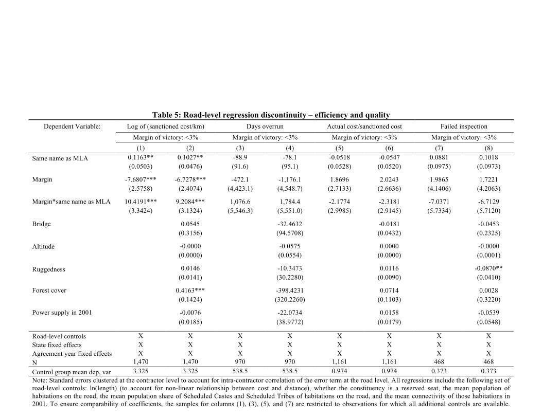
34

Table 5: Road-level regression discontinuity – efficiency and quality Dependent Variable: Log of (sanctioned cost/km) Days overrun Actual cost/sanctioned cost Failed inspection

Margin of victory: <3% Margin of victory: <3% Margin of victory: <3% Margin of victory: <3%

(1) (2) (3) (4) (5) (6) (7) (8) Same name as MLA 0.1163** 0.1027** -88.9 -78.1 -0.0518 -0.0547 0.0881 0.1018

(0.0503) (0.0476) (91.6) (95.1) (0.0528) (0.0520) (0.0975) (0.0973)

Margin -7.6807*** -6.7278*** -472.1 -1,176.1 1.8696 2.0243 1.9865 1.7221

(2.5758) (2.4074) (4,423.1) (4,548.7) (2.7133) (2.6636) (4.1406) (4.2063)

Margin*same name as MLA 10.4191*** 9.2084*** 1,076.6 1,784.4 -2.1774 -2.3181 -7.0371 -6.7129 (3.3424) (3.1324) (5,546.3) (5,551.0) (2.9985) (2.9145) (5.7334) (5.7120)

Bridge

0.0545

-32.4632 -0.0181 -0.0453

(0.3156)

(94.5708) (0.0432) (0.2325)

Altitude

-0.0000

-0.0575 0.0000 -0.0000

(0.0000)

(0.0554) (0.0000) (0.0001)

Ruggedness

0.0146

-10.3473 0.0116 -0.0870**

(0.0141)

(30.2280) (0.0090) (0.0410)

Forest cover

0.4163***

-398.4231 0.0714 0.0028

(0.1424)

(320.2260) (0.1103) (0.3220)

Power supply in 2001

-0.0076

-22.0734 0.0158 -0.0539

(0.0185)

(38.9772) (0.0179) (0.0548)

Road-level controls X X X X X X X X State fixed effects X X X X X X X X Agreement year fixed effects X X X X X X X X N 1,470 1,470 970 970 1,161 1,161 468 468 Control group mean dep, var 3.325 3.325 538.5 538.5 0.974 0.974 0.373 0.373 Note: Standard errors clustered at the contractor level to account for intra-contractor correlation of the error term at the road level. All regressions include the following set of road-level controls: ln(length) (to account for non-linear relationship between cost and distance), whether the constituency is a reserved seat, the mean population of habitations on the road, the mean population share of Scheduled Castes and Scheduled Tribes of habitations on the road, and the mean connectivity of those habitations in 2001. To ensure comparability of coefficients, the samples for columns (1), (3), (5), and (7) are restricted to observations for which all additional controls are available. Appendix Table A12 reports results for the respective optimal bandwidths derived from the optimal bandwidth choice rule of Imbens and Kalyanaraman (2011). *** p<0.01, ** p<0.05, * p<0.1

35

7. MECHANISMS

Our findings are consistent with recent work showing that MLAs have a significant impact on

economic outcomes in their constituency (Asher and Novosad 2017; Prakash et al. 2015), even

though the parliamentarians in question have limited official power. In the literature this

discrepancy between de jure responsibilities and de facto influence is often explained by

politicians’ informal control over the assignment of bureaucrats (Iyer and Mani, 2012).43

Bureaucrats have many ways to sway the allocation of contracts. The technical evaluation of bids

allows for discretion. In conversations with bureaucrats involved managing PMGSY tenders, we

were told that MLAs will often get technical requirements from bureaucrats and then share that

information with favoured contractors who then have a better chance of winning the tender

(Author interviews, April 12, 2016). In this section, we provide evidence for role of bureaucrats

as intermediaries. In particular, if bureaucrats are part of the corruption chain, we expect that (i)

“connected” bureaucrats facilitate corruption; and that (ii) bureaucrats who are under more

scrutiny are less inclined to facilitate corruption.

PMGSY tendering is generally administered at the district level. The highest ranking official

in a district is the District Collector (DC) – a member of the Indian Administrative Service

(IAS).44 It is likely that MLAs who have a connection to their district’s collector would find it

easier to influence the allocation of contracts. Applying our surname-matching approach we

therefore test for heterogeneity in our main result based on whether or not the DC and politician

have the same surname. We see such an alignment in 1.4% of the bureaucrat-election

observations. As bureaucrats are reassigned frequently, we split each constituency-term into

separate observations for each DC. Columns (1) to (4) of Table 6 show that the interaction

between winning an election and sharing the DC’s name is positive and significant at the optimal

bandwidth. The RD estimates lose precision in the smaller sample for the 3% bandwidth, but the 43The state’s chief minister (generally the head of the ruling party) is responsible for assigning top-level bureaucrats to districts and therefore has the most direct control over the bureaucracy. Asher and Novosad (2017) find that MLAs aligned with the party in power are able to influence the implementation of regulation in favour of local firms. In Appendix Table A14 we evaluate whether such MLAs have a greater influence over PMGSY contract allocation, with inconclusive results. The differential effect for aligned MLAs is consistently positive, but not statistically significant.44IAS officers’ executive record sheets provide data on the location and duration of their postings, allowing us to match DCs to districts, and by extension, to the constituencies in our sample. This data is available on the website of the Department of Personnel and Training: dopt.gov.in (accessed in December 2016).

36

magnitude of the coefficients is comparable. These results suggest that MLAs may engage in

more preferential allocation when the highest ranking bureaucrat is also a member of their

network. However, as the assignment of DCs may not be exogenous we cannot prove that this

result is causal.

Our second test exploits variation in the incentives which bureaucrats face over their career.

IAS officers are screened for promotion in their 13th and 16th years of service. The prospect of

higher positions and increased pay may cause them to improve their performance during these

periods. For example, Nath (2016) finds that DCs close to these promotion dates are faster at

approving local public good projects. To assess whether this dynamic applies here, we split each

constituency-term into separate observations for each DC who held office during the term. DC's

are reassigned frequently with a median tenure of 17 months. We define a DC as being subject to

promotion screening if their 13th or 16th year of service overlap with their tenure in a district.

The increase in connected contracts is, attenuated during such periods, as one would expect.

Columns (5) to (8) of Table 6 show that under a DC in their 13th or 16th year of service,

preferential allocation towards contractors who share the MLA’s name is much lower than when

the DC is not in those years and the point estimate is indistinguishable from zero.45 This could

reflect bureaucrats’ reluctance to participate in risky corruption, or greater monitoring of

improprieties on the part of their subordinates. Both channels suggest that political interference

involves the cooperation of bureaucrats.

In Table 7 we apply the same sources of variation to test for heterogeneity in our road-level

results. There is no evidence of a differential effect on the likelihood of a missing road or the

cost of the road for contracts allocated to contractors who share a surname with both the MLA

and the DC. However, when the DC is close to their promotion screening date, our results for

missing roads and for cost inflation are weaker. This is consistent with the idea that bureaucrats

up for promotion are less amenable to corrupt activities within their district.

45Appendix Table A15 shows that this result is robust to controlling for officers’ years of service and the interaction of years of service with winning the election. Columns (5) to (8) compare the effects in the promotion screening year to effects in prior and subsequent years. There is a weak negative effect in the year before promotion screening which may reflect anticipation of the screening process. The result is thus not due to some linear trend in DC behaviour; the attenuation in the effect of winning on the share of connected contractors appears to be specific to having a DC under the scrutiny that comes with evaluation for promotion.

37

The results of this section provide support for the hypothesis that local bureaucrats are a

crucial part of the chain that links politicians to the preferential allocation of contracts.

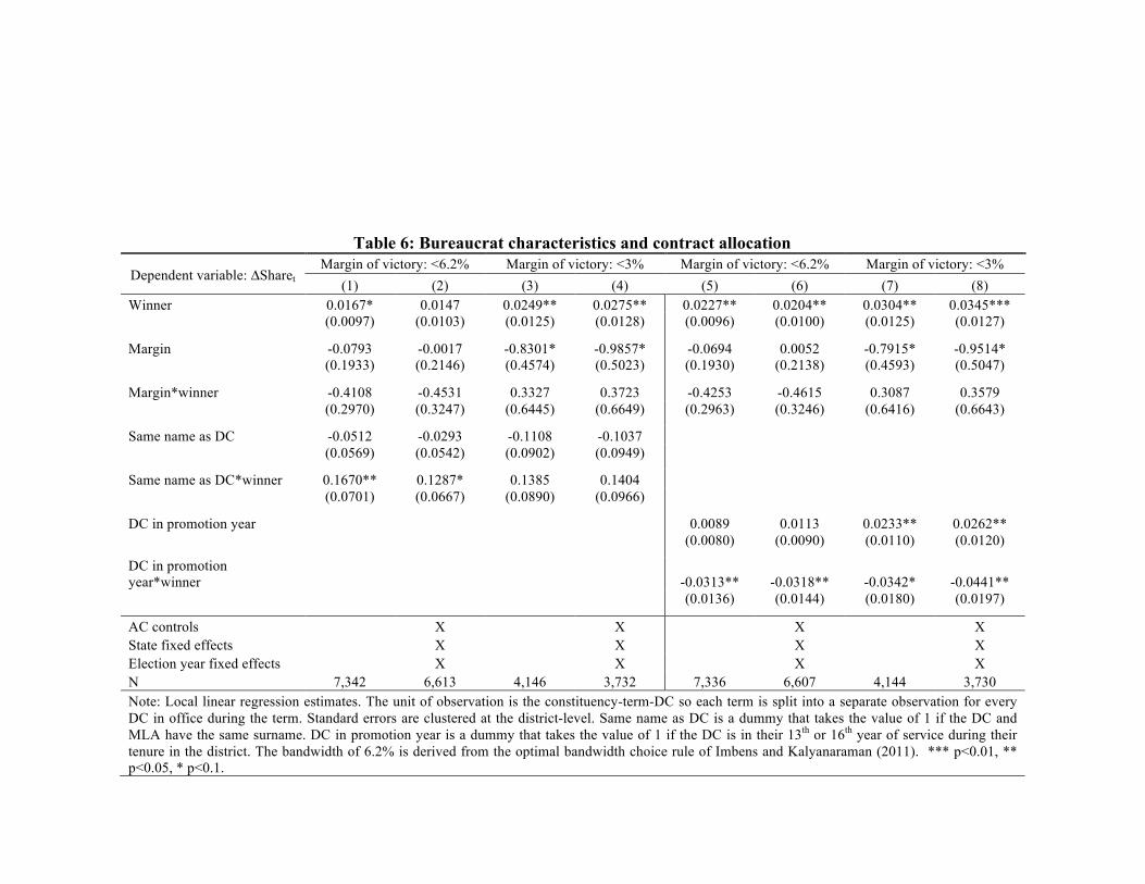
38

Table 6: Bureaucrat characteristics and contract allocation

Dependent variable: ΔSharet Margin of victory: <6.2% Margin of victory: <3% Margin of victory: <6.2% Margin of victory: <3%

(1) (2) (3) (4) (5) (6) (7) (8) Winner 0.0167* 0.0147 0.0249** 0.0275** 0.0227** 0.0204** 0.0304** 0.0345***

(0.0097) (0.0103) (0.0125) (0.0128) (0.0096) (0.0100) (0.0125) (0.0127)

Margin -0.0793 -0.0017 -0.8301* -0.9857* -0.0694 0.0052 -0.7915* -0.9514*

(0.1933) (0.2146) (0.4574) (0.5023) (0.1930) (0.2138) (0.4593) (0.5047)

Margin*winner -0.4108 -0.4531 0.3327 0.3723 -0.4253 -0.4615 0.3087 0.3579 (0.2970) (0.3247) (0.6445) (0.6649) (0.2963) (0.3246) (0.6416) (0.6643)

Same name as DC -0.0512 -0.0293 -0.1108 -0.1037

(0.0569) (0.0542) (0.0902) (0.0949)

Same name as DC*winner 0.1670** 0.1287* 0.1385 0.1404

(0.0701) (0.0667) (0.0890) (0.0966)

DC in promotion year

0.0089 0.0113 0.0233** 0.0262** (0.0080) (0.0090) (0.0110) (0.0120)

DC in promotion year*winner

-0.0313** -0.0318** -0.0342* -0.0441**

(0.0136) (0.0144) (0.0180) (0.0197)

AC controls

X

X

X X State fixed effects X X X X Election year fixed effects X X X X N 7,342 6,613 4,146 3,732 7,336 6,607 4,144 3,730 Note: Local linear regression estimates. The unit of observation is the constituency-term-DC so each term is split into a separate observation for every DC in office during the term. Standard errors are clustered at the district-level. Same name as DC is a dummy that takes the value of 1 if the DC and MLA have the same surname. DC in promotion year is a dummy that takes the value of 1 if the DC is in their 13th or 16th year of service during their tenure in the district. The bandwidth of 6.2% is derived from the optimal bandwidth choice rule of Imbens and Kalyanaraman (2011). *** p<0.01, ** p<0.05, * p<0.1.

39

Table 7: Bureaucrat characteristics and road outcomes Dependent Variable: Missing all-

weather road Missing road Log of

(sanctioned cost/km)

Missing all-weather road Missing road

Log of (sanctioned

cost/km)

(1) (2) (3) (4) (5) (6) Same name as MLA 0.2895*** 0.1504** 0.1126** 0.3885*** 0.1676** 0.1479***

(0.0978) (0.0649) (0.0467) (0.1068) (0.0779) (0.0569)

Margin -3.8176 -2.5438 -7.3982*** -7.4694 -1.8026 -7.8830***

(4.1530) (1.8993) (2.4709) (5.4338) (2.6045) (2.8675)

Margin*same name as MLA -4.2841 -1.3217 10.0164*** -1.9472 -2.7491 10.9856*** (5.2783) (2.7645) (3.2321) (6.5345) (3.3937) (3.6501)

Same name as DC 0.1144 0.0480 -0.0692

(0.0805) (0.0371) (0.0463)

Same name as DC*winner -0.0794 -0.0506 0.0148

(0.0961) (0.0457) (0.0587)

DC in promotion year

0.0262 0.0181 0.0261 (0.0862) (0.0253) (0.0393)

DC in promotion year*winner

-0.0911 -0.0990** -0.1303** (0.1160) (0.0472) (0.0603)

Road-level controls X X X X X X State fixed effects X X X X X X Agreement year fixed effects X X X X X X N 581 581 1,471 459 459 1,057 Note: Local linear regression estimates. Standard errors clustered at the contractor level to account for intra-contractor correlation of the error term at the road level. All regressions include the following set of road-level controls: ln(length), whether the constituency is a reserved seat, the mean population of habitations on the road, the mean population share of Scheduled Castes and Scheduled Tribes of habitations on the road, and the mean connectivity of those habitations in 2001. Same name as DC is a dummy that takes the value of 1 if the DC and MLA have the same surname. DC in promotion year is a dummy that takes the value of 1 if the DC is in their 13th or 16th year of service during their tenure in the district. The bandwidth of 6.2% is derived from the optimal bandwidth choice rule of Imbens and Kalyanaraman (2011). *** p<0.01, ** p<0.05, * p<0.1

40

8. ELECTORAL INCENTIVES FOR CORRUPTION

We implicitly assume that kinship ties to politicians are relevant connections in the structure of

local political corruption in India, and our results appear to validate this assumption. But why

should patronage be targeted along caste or familial lines? The literature offers two main

explanations: vote-buying and particularised trust. In this section we attempt to shed light on

which is more applicable to corruption in PMGSY

If road contracts are awarded in exchange for political contributions or political support, one

could expect the bias towards connected contractors to increase in election periods. To test for

this we construct more disaggregated measures of proximity: the share of contractors with a

candidate’s name in the first 12 months after an election (𝑠𝑡𝑎𝑟𝑡 𝑜𝑓 𝑡𝑒𝑟𝑚!"# .), the equivalent

share for the last 12 months before the subsequent election (𝑒𝑛𝑑 𝑜𝑓 𝑡𝑒𝑟𝑚!"#), and finally the

share for the intermediate, mid-term, period. The first three columns of Table 8 shows the results

of applying our main estimation approach to this disaggregated sample and interacting dummies

for 𝑠𝑡𝑎𝑟𝑡 𝑜𝑓 𝑡𝑒𝑟𝑚!"# and 𝑒𝑛𝑑 𝑜𝑓 𝑡𝑒𝑟𝑚!"# with 𝑤𝑖𝑛𝑛𝑒𝑟!"# . The overall effect of winning the

election is comparable to the term-level results, and we find no differential effects in election

years.

Although the bias towards connected contractors does not increase in election periods, there

could be different patterns for the within-term variation on the cost margin. Politicians might

need to extract rents, buy support, or reward supporters more before or after elections. Including

the interactions between 𝑠𝑎𝑚𝑒 𝑛𝑎𝑚𝑒 𝑎𝑠 𝑀𝐿𝐴!"# and 𝑠𝑡𝑎𝑟𝑡 𝑜𝑓 𝑡𝑒𝑟𝑚!"# and 𝑒𝑛𝑑 𝑜𝑓 𝑡𝑒𝑟𝑚!"# in

the road-level regressions, we again find no evidence of a political cycle in which election

periods see increased corruption (columns 4-6 of Table 8). The observed negative effect for both

the start and end of term is more consistent with increased scrutiny in the run-up to elections

acting as a deterrent to corruption.

41

Table 8: Three tests for electioneering

Dependent variable: ΔSharet in cols 1-3 and 7 Log of (sanctioned cost/km) in cols 4-6

Electoral cycles: allocation Electoral cycles: cost Effect in “politically irrelevant”

areas Start of term heterogeneity

End of term heterogeneity

Start and end of term

heterogeneity

Start of term heterogeneity

End of term heterogeneity

Start and end of term

heterogeneity (1) (2) (3) (4) (5) (6) (7)

Winner (Same name as MLA in cols 4-6)

0.0328** 0.0350** 0.0344** 0.1166** 0.1359*** 0.1433*** 0.0250* (0.0155) (0.0152) (0.0160) (0.0518) (0.0525) (0.0540) (0.0146)

Margin -1.1660* -1.1466 -1.1591* -7.0964*** -7.6324*** -7.0332*** -0.2272 (0.6971) (0.6969) (0.6971) (2.5415) (2.6163) (2.5659) (0.5518) Margin*winner (Margin*same name as MLA in cols 4-6)

0.8036 0.7620 0.7868 9.8967*** 10.3096*** 9.7854*** -0.0918 (0.7374) (0.7388) (0.7390) (3.2878) (3.3607) (3.2915) (0.7128)

Start of term -0.0091

-0.0119 0.1270*** 0.1420***

(0.0083)

(0.0086) (0.0422) (0.0444)

Start of term*winner (Start of term*same name as MLA in cols 4-6)

0.0029

0.0013 -0.0746 -0.0973*

(0.0111)

(0.0112) (0.0546) (0.0552)

End of term

-0.0040 -0.0089 0.0521 0.0796

(0.0074) (0.0075) (0.0568) (0.0581)

End of term*winner (End of term*same name as MLA in cols 4-6)

-0.0050 -0.0044 -0.1303** -0.1480*** (0.0114) (0.0114) (0.0551) (0.0553)

Politically irrelevant*post announcement*winner -0.0273 (0.0218) Constituency controls X X X X X X X Candidate controls X X X X Road-level controls X X X State and agreement year fixed effects X X X X X X X N 3,201 3,201 3,201 1,470 1,470 1,470 2,707Note: Terms in the sample for columns 1-3 are disaggregated by time: first year, last year, and remaining period. Terms in the sample for column 7 are disaggregated by time (pre- and post- the announcement of delimitation) and spatially (based on intra-constituency boundaries introduced by delimitation). The RD bandwidth for all columns is 3%. Appendix Tables A16-18 reports the equivalent results for the respective optimal bandwidths derives from the optimal bandwidth rule of Imbens and Kalyanaraman (2011). Standard errors are clustered at the election level in columns 1-3 and 7 and at the contractor level in columns 4-6. Controls for columns 1-3 and 7 are the same as in Table 3. Controls for columns 4-6 are the same as in Tables 4 and 5. Regression in column 7 includes all lower-order interactions (not reported). All regressions include a constant. *** p<0.01, ** p<0.05, * p<0.1

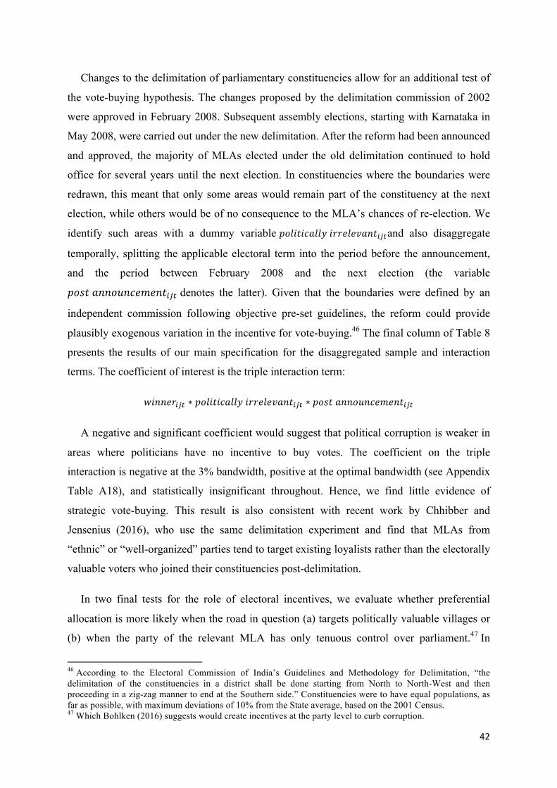
42

Changes to the delimitation of parliamentary constituencies allow for an additional test of

the vote-buying hypothesis. The changes proposed by the delimitation commission of 2002

were approved in February 2008. Subsequent assembly elections, starting with Karnataka in

May 2008, were carried out under the new delimitation. After the reform had been announced

and approved, the majority of MLAs elected under the old delimitation continued to hold

office for several years until the next election. In constituencies where the boundaries were

redrawn, this meant that only some areas would remain part of the constituency at the next

election, while others would be of no consequence to the MLA’s chances of re-election. We

identify such areas with a dummy variable 𝑝𝑜𝑙𝑖𝑡𝑖𝑐𝑎𝑙𝑙𝑦 𝑖𝑟𝑟𝑒𝑙𝑒𝑣𝑎𝑛𝑡!"#and also disaggregate

temporally, splitting the applicable electoral term into the period before the announcement,

and the period between February 2008 and the next election (the variable

𝑝𝑜𝑠𝑡 𝑎𝑛𝑛𝑜𝑢𝑛𝑐𝑒𝑚𝑒𝑛𝑡!"# denotes the latter). Given that the boundaries were defined by an

independent commission following objective pre-set guidelines, the reform could provide

plausibly exogenous variation in the incentive for vote-buying.46 The final column of Table 8

presents the results of our main specification for the disaggregated sample and interaction

terms. The coefficient of interest is the triple interaction term:

𝑤𝑖𝑛𝑛𝑒𝑟!"# ∗ 𝑝𝑜𝑙𝑖𝑡𝑖𝑐𝑎𝑙𝑙𝑦 𝑖𝑟𝑟𝑒𝑙𝑒𝑣𝑎𝑛𝑡!"# ∗ 𝑝𝑜𝑠𝑡 𝑎𝑛𝑛𝑜𝑢𝑛𝑐𝑒𝑚𝑒𝑛𝑡!"#

A negative and significant coefficient would suggest that political corruption is weaker in

areas where politicians have no incentive to buy votes. The coefficient on the triple

interaction is negative at the 3% bandwidth, positive at the optimal bandwidth (see Appendix

Table A18), and statistically insignificant throughout. Hence, we find little evidence of

strategic vote-buying. This result is also consistent with recent work by Chhibber and

Jensenius (2016), who use the same delimitation experiment and find that MLAs from

“ethnic” or “well-organized” parties tend to target existing loyalists rather than the electorally

valuable voters who joined their constituencies post-delimitation.

In two final tests for the role of electoral incentives, we evaluate whether preferential

allocation is more likely when the road in question (a) targets politically valuable villages or

(b) when the party of the relevant MLA has only tenuous control over parliament.47 In

46 According to the Electoral Commission of India’s Guidelines and Methodology for Delimitation, “the delimitation of the constituencies in a district shall be done starting from North to North-West and then proceeding in a zig-zag manner to end at the Southern side.” Constituencies were to have equal populations, as far as possible, with maximum deviations of 10% from the State average, based on the 2001 Census. 47 Which Bohlken (2016) suggests would create incentives at the party level to curb corruption.

43

Appendix Tables A19 and A20 we find no evidence that the likelihood of MLA interference

depends on the political significance of destination villages (as proxied by having the

Panchayat headquarters, which may make them more valuable, or majority SC/ST population,

which can make them less so, particularly in unreserved constituencies) or that aligned MLAs

engage in less corruption when their party’s control of parliament is more precarious (as

measured by its seat share). The fact that we find no variation based on political incentives is

further evidence to suggest that corrupt contract allocations are not motivated by vote-buying.

In the absence of clear evidence for vote buying, it is possible that corruption arises within

kinship networks because these provide the “particularised trust” needed to engage in risky

collusive behaviour (Tonoyan, 2003). While we are unable to test this explanation explicitly,

it fits the context of PMGSY in that the involvement of the central government provides a

minimum level of monitoring. Given this supervision, it is notable that we only find evidence

of corruption in certain aspects of the programme. Our results suggest that preferential

allocation adversely affects every performance marker except the two that are most easily

observed in the central administrative data: over-runs and delays. This is in line with the idea

that contractors face a trade-off between potential rents and the cost of detection. Similarly,

we find that preferentially allocated contracts are less expensive in the period before elections,

when scrutiny may be higher and detection is more damaging to politicians. The overall

pattern of our results is therefore consistent with a setting in which politicians, bureaucrats,

and contractors are constrained by monitoring and operate on the least risky margins and with

the least risky collaborators – the members of their family or caste network.

The introduction of e-procurement for PMGSY also allows us to evaluate the effect of an

intervention that increased the monitoring capacity of higher level officials. Lewis-Faupel et

al. (2016) find that e-procurement improved the quality of PMGSY road construction. They

identify the entry of higher quality contractors from outside regions as a key mechanism

behind the quality improvement. However, we find no evidence that e-procurement has

helped to prevent the specific form of corruption we document in this paper.48 This null result

is consistent with corrupt practices being relatively sophisticated in the context of PMGSY,

even before e-tendering.

A distinguishing feature of PMGSY is that the programme has been subject to a central

monitoring system from its inception. However, by explicitly prohibiting political 48 These results are reported in the Appendix (Table A21).

44

involvement, it foregoes a mechanism that could provide local accountability. If voters held

their MLAs responsible for the services delivered under PMGSY, the latter would have an

incentive to limit corruption. By contrast, a scheme in which local politicians have no formal

role but over which they still retain influence through informal channels, can be seen as an

ideal vehicle for rent-seeking. Our results provide mixed evidence on electoral accountability.

While cost overruns are weaker around elections, the preferential allocation does not show

any electoral cycle. One interpretation of these findings is that PMGSY limited political

control in the allocation of contracts, but that this came at the expense of reduced political

accountability. While we cannot test this trade-off directly in our context, we believe it is an

interesting avenue for future research.

9. CONCLUSION

This paper provides direct empirical evidence that local politicians in India abuse their power

to benefit members of their own network. We exploit the variation in political leadership due

to the electoral cycle, to identify systematic distortions in the allocation of contracts for a

major rural road construction programme (PMGSY). By matching contractors’ and political

candidates’ surnames, we generate a measure of proximity which evolves as the pool of

contractors changes. A regression discontinuity design based on close elections, suggests that

the causal impact of a politician coming to power is an 83% increase in the share of roads

allocated to contractors who share their surname.

This result withstands a series of alternative specifications and robustness checks. Further

regression discontinuity estimates at the road level, indicate that corruption is welfare-

reducing in this context. Political interference is associated with higher costs and a greater

likelihood that roads go missing. While constituencies with close elections are clearly in a

different political equilibrium (close elections are contested by more candidates, for example),

a difference-in-differences estimate for the whole sample also shows a positive and

statistically significant increase in the share of connected contacts, albeit a smaller one than

in the RD specification. This finding suggests that the LATE we estimate in the RD has

external validity.

A distinguishing feature of our analysis, is that we identify the effect of political

connections to state-level legislators who have no official involvement in the road

45

construction programme. Our results therefore not only indicate preferential treatment of the

politically connected, they also provide indirect evidence that local politicians’ power over

purportedly neutral bureaucrats is sufficient to coerce them into corruption. From a policy

perspective, these findings indicate that more could be done to insulate the officials

implementing government programmes at the local level, including those involved in

PMGSY. The result that misallocation is lower and contract performance is better for

bureaucrats who face promotion incentives, points in this direction.

A striking feature of PMGSY is that the bidding rules were designed explicitly to limit

political influence. However, such anti-corruption measures could face a trade-off between

political accountability and political control. If voters believe the limitations work, then a

logical conclusion would be that their MLAs are not responsible for poor programme

performance. While we find some evidence that cost inflation is weaker around election times,

our preferential allocation results remain very stable throughout the electoral cycle. These

findings are consistent with the idea that the limited control of politicians over PMGSY could

have come at the expense of reduced accountability to voters.

While this paper is primarily about the measurement and mechanisms of corruption, its

findings have significance beyond the potential number of misallocated roads or the amount

of misdirected funds. If corrupt arrangements were made based on random matching between

individuals, the empirical strategy would have revealed nothing. Our results provide further

evidence for the role of networks in enabling corruption and point towards theories in which

kinship networks facilitate corruption through trust or the ability to impose social sanctions.

The irony is, that the setting for the analysis – PMGSY – is conceptually a profoundly

inclusive programme, facilitating the integration of over 100 million people into the Indian

economy (Aggarwal 2017). This paper suggests that allowing them to compete equally for

jobs, permits, licenses, or government procurement contracts, may require building more than

roads.

46

ACKNOWLEDGEMENTS

We would like to thank the International Growth Centre (IGC) and CEPREMAP for

supporting the data collection of this project. We are also grateful to Nawal Agrarwal, Ashish

Modi, Anukriti Ranjan, Shrenik Sanghvi, Radha Sarkar, and Paolo Santini for excellent

research assistance. This paper has benefited from discussions with Sam Asher, Anjali

Bohlken, Tarek Ghani, Guy Grossman, Dan Keniston, Ariane Lambert-Mogilianski, Karen

Macours, Alexander Plekhanov, Akiko Suwa-Eisenmann, Liam Wren-Lewis, and Maiting

Zhuang, as well as excellent feedback from our anonymous referees and the editor. We also

thank seminar participants in PSE’s IRG and India-China Workshops, the Namur Indian

Political Economy Workshop, the Graduate Institute (Geneva), and the Sussex Development

Workshop. All remaining errors are our own.

REFERENCES Acemoglu, Daron, Tarek Hassan, and Ahmed Tahoun. “The Power of the Streets: Evidence

from Egypt’s Arab Spring.” Mimeo MIT (2014).

Aggarwal, Shilpa. "Do rural roads create pathways out of poverty? Evidence from India." Mimeo (2017).

Amore, Mario Daniele, and Morten Bennedsen. "The value of local political connections in a low-corruption environment." Journal of Financial Economics110, no. 2 (2013): 387-402.

Angelucci, Manuela, Giacomo De Giorgi, Marcos A. Rangel, and Imran Rasul. "Family networks and school enrolment: Evidence from a randomized social experiment." Journal of Public Economics 94, no. 3 (2010): 197-221.

Asher, Sam, and Paul Novosad. "Politics and Local Economic Growth: Evidence from India." American Economic Journal: Applied Economics 9, no. 1(2017): 229-273.

Asher, Sam, and Paul Novosad. "Market Access and Structural Transformation: Evidence from Rural Roads in India." Manuscript: Department of Economics, University of Oxford (2016).

Banerjee, Abhijit, Sendhil Mullainathan, and Rema Hanna. "Corruption" Handbook of Organizational Economics, Princeton University Press, (2013).

Banerjee, Abhijit, Donald P. Green, Jeffery McManus, and Rohini Pande. "Are poor voters indifferent to whether elected leaders are criminal or corrupt? A vignette experiment in rural India." Political Communication 31, no. 3 (2014): 391-407.

Becker, Gary S., and George J. Stigler. "Law enforcement, malfeasance, and compensation of enforcers." The Journal of Legal Studies (1974): 1-18.

47

Bertrand, Marianne, Simeon Djankov, Rema Hanna, and Sendhil Mullainathan. "Obtaining a driver's licesnse in India: an experimental approach to studying corruption." The Quarterly Journal of Economics (2007): 1639-1676.

Bobonis, Gustavo J., Luis Camara Fuertes, Raier Schwabe, "Monitoring Corruptible Politicians.", American Economic Review 106, no. 8 (2016): 2317-2405.

Bohlken, Anjali Thomas. "Development or Rent-seeking: How Political Influence Shapes Infrastructure Provision in India", Mimeo (2016).

Bussell, Jennifer. "Clients or Constituents? Distribution Between the Votes in India." mimeo, University of California Berkeley (2015)

Caughey, Devin, and Jasjeet S. Sekhon. "Elections and the regression discontinuity design: Lessons from close us house races, 1942–2008." Political Analysis 19, no. 4 (2011): 385-408.

Chandra, Kanchan. "Why Ethnic Parties Suceed." Patronage and ethnic head counts in India (2004).

Chhibber, Pradeep, and Francesca R. Jensenius. 2016. “Privileging one’s own? Voting patterns and politicized spending in India.” Mimeo.

Chopra, Vir K. Marginal players in marginal assemblies: The Indian MLA. Orient Longman, 1996.

Cingano, Federico, and Paolo Pinotti. “Politicians at Work: The private Returns and Social Costs of Policial Connections.” Journal of the European Economic Association, Vol. 11, No.2 (2013), p.433-465.

Do, Quoc-Anh, Yen Teik Lee, and Bang Dang Nguyen. "Political connections and firm value: evidence from the regression discontinuity design of close gubernatorial elections." CEPR Discussion Paper No. 10526 (2015).

Eggers, Andrew C. and Jens Hainmueller, “MPs For Sale: Returns to Office in Post-War British Politics”, American Political Science Review, Vol. 103, No. 4, (2009): pp. 1-21.

Eggers, Andrew C., Anthony Fowler, Jens Hainmueller, Andrew B. Hall, and James M. Snyder. "On the validity of the regression discontinuity design for estimating electoral effects: New evidence from over 40,000 close races." American Journal of Political Science 59, no. 1 (2015): 259-274.

Fafchamps, Marcel, and Julien Labonne. "Do politicians’ relatives get better jobs? Evidence from Municipal Elections." The Journal of Law, Economics, and Organization 33, no. 2 (2017): 268-300.

Ferraz, Claudio, and Federico Finan. "Exposing corrupt politicians: the effects of Brazilians publicly released audits on electoral outcomes." Quarterly Journal of Economics 123, no. 3 (2008): 703.

Ferraz, Claudio, and Frederico Finan. "Electoral Accountability and Corruption: Evidence from the Audits of Local Government." American Economic Review 101 (2011): 1274.

Field, Erica, Matthew Levinson, Rohini Pande, and Sujata Visaria. "Segregation, Rent Control, and Riots: The Economics of Religious Conflict in an Indian City." The American Economic Review (2008): 505-510.

Fisman, Raymond. "Estimating the value of political connections." American Economic Review (2001): 1095-1102.

48

Fisman, Raymond, Florian Schulz, and Vikrant Vig. “Private Returns to Public Office”. Journal of Political Economy (2014).

Fisman, Raymond, and, Yongxiang Wang. “The Mortality Cost of Political Connections.” Review of Economic Studies. Vol. 83, No. 4 (2015).

Fisman, Raymond, Daniel Paravisini, and Vikrant Vig. "Cultural proximity and loan outcomes." The American Economic Review 107, no. 2 (2017): 457-492.

Golden, Miriam A., and Lucio Picci. "Proposal for a new measure of corruption, illustrated with Italian data." Economics & Politics 17, no. 1 (2005): 37-75.

Gulzar, Saad, and Ben Pasquale. “Politicians, Bureaucrats, and Development: Evidence from India.” American Political Science Review (2016).

Hoff, Karla, and Priyanka Pandey. “Belief System and Durable Inequalities: An Experimental Investigation of Indian Caste.” World Bank, Policy Research Paper: No. 3351, 2004.

Horowitz, Donald L. Ethnic groups in conflict. Univ of California Press, 1985. Huntington, S. "Modernisation and Corruption ‘in Political Order in Changing Societies,

Yale University Press, New Havern." (1968). Imbens, Guido, and Karthik Kalyanaraman. "Optimal bandwidth choice for the regression

discontinuity estimator." The Review of Economic Studies (2011). Iyer, Lakshmi, and Anandi Mani. "Traveling agents: political change and bureaucratic

turnover in India." Review of Economics and Statistics 94, no. 3 (2012): 723-739. Jensenius, Francesca Refsum. "Power, performance and bias: Evaluating the electoral quotas

for scheduled castes in India." (2013). PhD Thesis, University of California Berkeley Krueger, Anne O. "The political economy of the rent-seeking society." The American

economic review (1974): 291-303. Khwaja, Asim Ijaz, and Atif Mian. “Do Lenders Favor Politically Connected Firms? Rent

Provision in and Emerging Financial Market.” Quarterly Journal of Economics. Vol. 120, No. 4 (2005). 1371-1411.

Lambsdorff, Johann Graf. "Corruption and rent-seeking." Public choice 113, no. 1-2 (2002): 97-125.

Larreguy, Horacio A., John Marshall, and James M. Snyder Jr. Revealing Malfeasance: How Local Media Facilitates Electoral Sanctioning of Mayors in Mexico. No. w20697. National Bureau of Economic Research, 2014.

Lee, David S. "Randomized experiments from non-random selection in US House elections." Journal of Econometrics 142, no. 2 (2008): 675-697.

Lee, David S., and Thomas Lemieux. "Regression Discontinuity Designs in Economics." Journal of Economic Literature 48 (2010): 281-355.

Leff, Nathaniel H. "Economic development through bureaucratic corruption."American behavioral scientist, 8, no. 3 (1964): 8-14.

Lewis-Faupel, Sean, Yusuf Neggers, Benjamin A. Olken, and Rohini Pande. "Can Electronic Procurement Improve Infrastructure Provision? Evidence from Public Works in India and Indonesia," American Economic Journal: Economic Policy, (2016).

Lui, Francis T. "An equilibrium queuing model of bribery." The journal of political economy (1985): 760-781.

49

Mastrobuoni, Giovanni, and Eleonora Patacchini. "Organized crime networks: An application of network analysis techniques to the American mafia." Review of Network Economics 11, no. 3 (2012).

McCrary, Justin. "Manipulation of the running variable in the regression discontinuity design: A density test." Journal of Econometrics 142, no. 2 (2008): 698-714.

Melo, Marcus André, Carlos Pereira, and Carlos Mauricio Figueiredo. "Political and institutional checks on corruption: Explaining the performance of Brazilian audit institutions." Comparative Political Studies (2009).

Mironov, Maxim and Ekaterina Zhuravskaya. 2016. "Corruption in Procurement and the Political Cycle in Tunneling: Evidence from Financial Transactions Data." American Economic Journal: Economic Policy, 8(2): 287-321.

Nath, Anusha. "Bureaucrats and Politicians: How Does Electoral Competition Affect Bureaucratic Performance?" Institute for Economic Development (IED) Working Paper 269 (2016).

NRRDA, “Pradhan Mantri Gram Sadak Yojana Operations Manual.” (2005). NRRDA, “Standard Bidding Document for PMGSY.” (2015).

Olken, Benjamin A., and Patrick Barron. "The Simple Economics of Extortion: Evidence from Trucking in Aceh." Journal of Political Economy 117 (3) (2009).

Olken, Benjamin A. “Monitoring Corruption: Evidence from a Field Experiment in Indonesia” Journal of Political Economy 115 (2) (2007): 200-249

Oster, Emily. "Unobservable selection and coefficient stability: Theory and evidence." Journal of Business and Economic Statistics, forthcoming (2017).

Prakash, Nishith, Marc Rockmore, and Yogesh Uppal. 2015. “Do criminally accused politicians affect economic outcomes? Evidence from India”, Mimeo.

Reinikka, Ritva, and Jakob Svensson. "Local capture: evidence from a central government transfer program in Uganda." The Quarterly Journal of Economics (2004): 679-705.

Rose-Ackerman, Susan. "The economics of corruption." Journal of public economics 4, no. 2 (1975): 187-203.

Shleifer, Andrei, and Robert W. Vishny. "Corruption.” The Quarterly Journal of Economics 108, no. 3 (1993): 599-617

Sukhtankar, Sandip. "Sweetening the deal? Political connections and sugar mills in India." American Economic Journal: Applied Economics 4, no. 3 (2012): 43-63.

Sukhtankar, Sandeep. “The Impact of Corruption on Consumer Markets: Evidence from the Allocation of Second-Generation Wireless Spectrum in India.” The Journal of Law and Economics, Vol. 58, No. 1. (2015).

Tonoyan, Vartuhí. "Corruption and Entrepreneurship: Impact of Trust and Civic Society; a Cross Cultural Comparison of 21 Countries; Paper Presented at the International Conference on" Trust and Entrepreneurial Behavior in East and West European Economies: Concepts, Developments and Comparative Aspects", University of Bremen 2003." ifm, 2003.

50

World Bank, “PMGSY Rural Roads Project : P124639 - Implementation Status Results Report” (2014).

Truex, R. “The returns to office in a ‘rubber stamp’ parliament”, American Political Science Review, 108, no.2 (2014): 235-251.

Vissa, Balagopal. "A matching theory of entrepreneurs' tie formation intentions and initiation of economic exchange." Academy of Management Journal 54, no. 1 (2011): 137-158.

i

FOR ONLINE PUBLICATION:

FIGURES

Figure A1: graphical depiction of the McCrary test

Note: This figure plots the McCrary test. The running variable in this analysis is continuously distributed by construction. The test is performed on an alternative version of the margin variable: the margin of victory for the candidate with the higher level of 𝑠ℎ𝑎𝑟𝑒!"#!!.

02

46

8

-1 -.5 0 .5

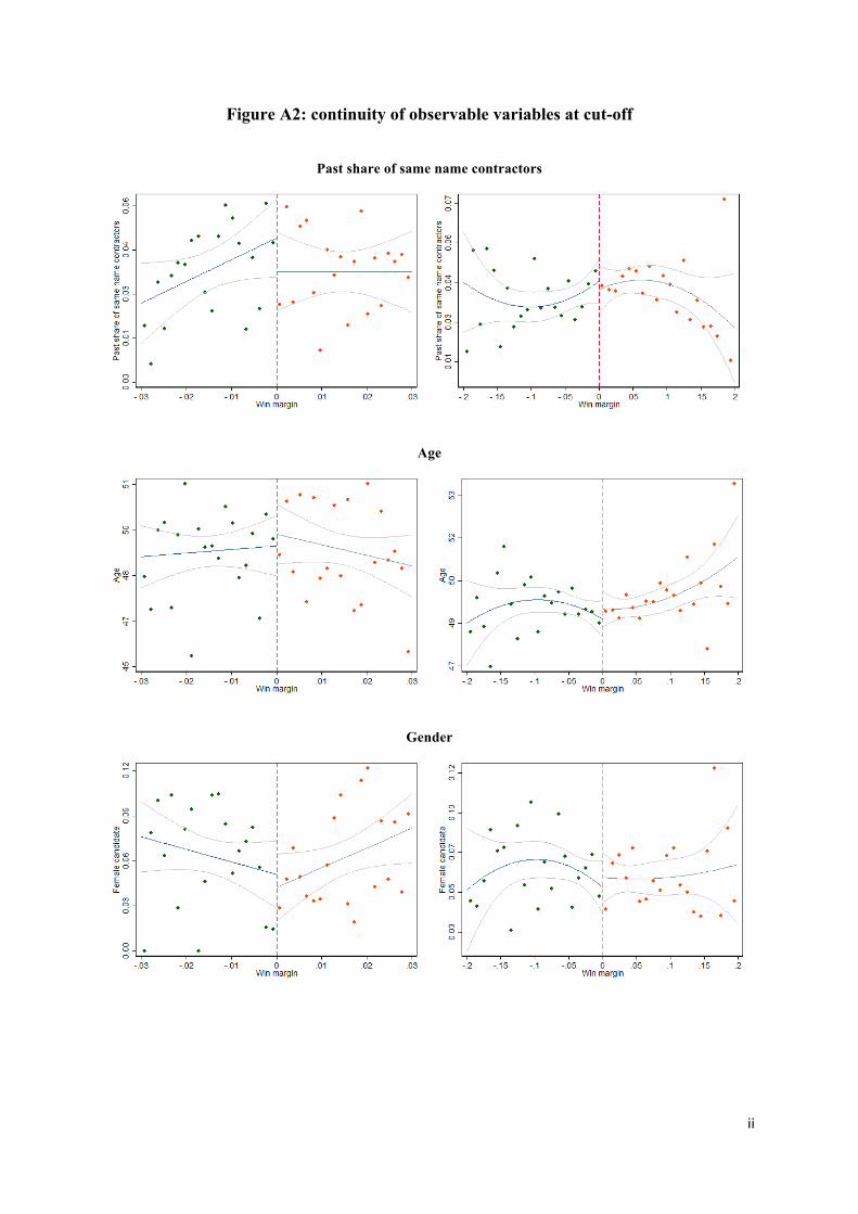
ii

Figure A2: continuity of observable variables at cut-off

Past share of same name contractors

Age

Gender

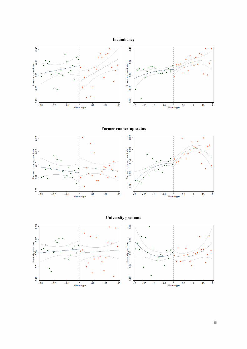
iii

Incumbency

Former runner-up status

University graduate

iv

INC candidate

BJP candidate

Note: Lines fitted separately on the samples left and right of the cut-off. Each dot represents the mean for a bin. The number of observations in a bin varies, based on the density of candidates at a given margin. 90% confidence intervals plotted in grey. The first panel shows a linear fit within the 3% bandwidth used in the RD estimation. The second shows a quadratic fit for a wider margin of 20%.

v

MAPS

Map 1: Constituencies in Sample Map 2: Constituencies with close elections

Note: The constituencies shown on maps are based on the pre-2008 delimitation. Post delimitation data is assigned to pre-delimitation boundaries. In Map 1 all constituencies with consecutive electoral terms with PMGSY road construction are shaded blue. In Map 2 constituencies with at least one election with a margin of victory lower than 6.2% (derived from the optimal bandwidth choice rule of Imbens and Kalyanaraman (2011)) are shaded red.

Map 3: Variation in the baseline share of same name contractors

Note: The constituencies shown on maps are based on the pre-2008 delimitation. Post delimitation data is assigned to pre-delimitation boundaries. Map 3 plots 𝑠ℎ𝑎𝑟𝑒!"# for all constituencies in the sample. Darker shades indicate a higher value of 𝑠ℎ𝑎𝑟𝑒!"#.

vi

TABLES

Table A1: Sources of election data

Source Years covered No. of elections No. of candidates Candidate-level variables

used in the sample

ECI digitised data 2005-2014 7,328 80,323 name, vote share, gender,

party

Bhavani (2012) 1977-2012 31,422 300,087 name, vote share, gender,

party

Empowering India 1951-2015 19,715 196,935 assets, education, age

National Election Watch

2004-2015 8,944 73,200 assets, liabilities, education,

criminal charges

Note: ECI digitised data refers to a subset of the ECI data that are available online at eci.nic.in. Bhavani (2012) is a dataset kindly made public by Rikhil R. Bhavnani. Empowering India and National Election Watch are NGOs. Their data is accessible at www.empoweringindia.com and myneta.info respectively. Where a variable is listed twice in the fifth column, this is due to incomplete time series or missing values that are filled in by drawing on multiple datasets.

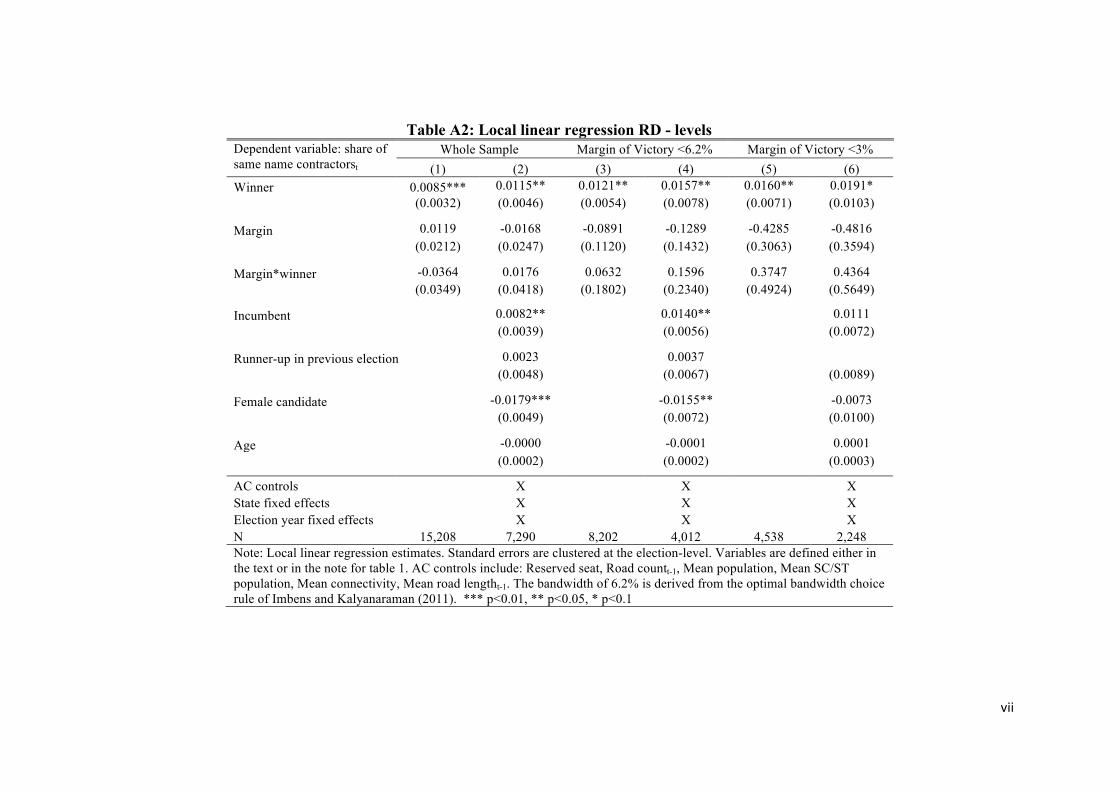
vii

Table A2: Local linear regression RD - levels Dependent variable: share of same name contractorst

Whole Sample Margin of Victory <6.2% Margin of Victory <3% (1) (2) (3) (4) (5) (6)

Winner 0.0085*** 0.0115** 0.0121** 0.0157** 0.0160** 0.0191* (0.0032) (0.0046) (0.0054) (0.0078) (0.0071) (0.0103)

Margin 0.0119 -0.0168 -0.0891 -0.1289 -0.4285 -0.4816

(0.0212) (0.0247) (0.1120) (0.1432) (0.3063) (0.3594)

Margin*winner -0.0364 0.0176 0.0632 0.1596 0.3747 0.4364 (0.0349) (0.0418) (0.1802) (0.2340) (0.4924) (0.5649)

Incumbent 0.0082** 0.0140** 0.0111 (0.0039) (0.0056) (0.0072)

Runner-up in previous election 0.0023 0.0037 (0.0048) (0.0067) (0.0089)

Female candidate -0.0179*** -0.0155** -0.0073 (0.0049) (0.0072) (0.0100)

Age -0.0000 -0.0001 0.0001 (0.0002) (0.0002) (0.0003)

AC controls

X

X

X State fixed effects X X X Election year fixed effects X X X N 15,208 7,290 8,202 4,012 4,538 2,248 Note: Local linear regression estimates. Standard errors are clustered at the election-level. Variables are defined either in the text or in the note for table 1. AC controls include: Reserved seat, Road countt-1, Mean population, Mean SC/ST population, Mean connectivity, Mean road lengtht-1. The bandwidth of 6.2% is derived from the optimal bandwidth choice rule of Imbens and Kalyanaraman (2011). *** p<0.01, ** p<0.05, * p<0.1

viii

Table A3: Balance test at 3% bandwidth Obs Mean winner Mean runner-up P value (1) (2) (3) (4) Panel A: Candidate characteristicsSharet-1 2472 0.038 0.038 0.913 Incumbent 2472 0.274 0.278 0.8221 Runner-up in prev. election 2472 0.144 0.140 0.7734 Age 2314 48.853 48.806 0.9114 Female candidate 2472 0.061 0.063 0.8679 Cand. faces criminal charge 1889 0.220 0.220 0.990 Assets (INR millions) 1554 386.0 220.0 0.7005 Liabilities (INR millions) 1747 1.218 1.415 0.54 University degree 1747 0.598 0.602 0.8377 Post-grad. degree 1747 0.207 0.196 0.5706 BJP candidate 2465 0.257 0.281 0.192 Congress candidate 2461 0.208 0.185 0.1587 Panel B: Share of roads built by contractors of same name in term prior to election Share 5 yrs before election 1416 0.033 0.027 0.4586 Share 4 yrs before election 1624 0.033 0.041 0.3478 Share 3 yrs before election 1490 0.032 0.037 0.5861 Share 2 yrs before election 942 0.031 0.035 0.709 Share 1 year before election 1070 0.036 0.049 0.2334 Panel C: Prevalence of most common names Named Kumar 2472 0.070 0.061 0.3701 Named Lal 2472 0.028 0.027 0.9015 Named Patel 2472 0.011 0.011 0.8466 Named Ram 2472 0.018 0.020 0.6588 Named Reddy 2472 0.013 0.008 0.237 Named Singh 2472 0.134 0.120 0.2771 Named Yadav 2472 0.019 0.019 0.883 Note: Variables are defined as in Table 1. Columns 2 and 3 show the respective means for winners and runners-up at the 3% bandwidth. *** p<0.01, ** p<0.05, * p<0.1

ix

Table A4: Fully non-parametric RD

Dep. Variable: ΔShare of same name contractorst

Whole Sample Margin of Victory <6.2% Margin of Victory <3%

(1) (2) (3) (4) (5) (6) Winner 0.0090** 0.0090** 0.0100** 0.0108** 0.0146** 0.0145**

(0.0035) (0.0037) (0.0049) (0.0051) (0.0065) (0.0069)

Incumbent -0.0015 0.0028 -0.0056 (0.0045) (0.0065) (0.0085)

Runner-up in previous election 0.0068 0.0067 0.0027 (0.0055) (0.0078) (0.0110)

Female candidate -0.0011 -0.0131 -0.0012 (0.0065) (0.0107) (0.0117)

Age 0.0002 -0.0000 0.0004 (0.0002) (0.0003) (0.0003)

AC controls

X

X

X State fixed effects X X X Election year fixed effects X X X N 8,116 7,290 4,396 4,012 2,472 2,248 Note: Local linear regression estimates. Standard errors are clustered at the election-level. Variables are defined either in the text or in the note for table 1. AC controls include: Reserved seat, Road countt-1, Mean population, Mean SC/ST population, Mean connectivity, Mean road lengtht-1. The bandwidth of 6.2% is derived from the optimal bandwidth choice rule of Imbens and Kalyanaraman (2011). *** p<0.01, ** p<0.05, * p<0.1

x

Table A5: Change in Sharet for losing candidates

Dependent variable: share of same name contractorst

Whole Sample Margin of Victory <6.2%

Margin of Victory <3%

(1) (2) (3) Post election -0.0035 -0.0060 -0.0073 (0.0027) (0.0037) (0.0053)

Margin -0.0211 0.0620 0.2091 (0.0240) (0.1363) (0.3318)

Candidate controls X X X AC controls X X X State fixed effects X X X Election year fixed effects X X X N 6,291 3,446 1,918 Note: OLS estimates. This sample is restricted to candidates who finished second in their elections. Post election is a dummy that takes the value of 0 for the term prior to the election and the value of 1 for the term after the election. The list of candidate and constituency controls is the same as in Table 3. The bandwidth of 6.2% is derived from the optimal bandwidth choice rule of Imbens and Kalyanaraman (2011). *** p<0.01, ** p<0.05, * p<0.1

Table A6: Allocation results dropping candidates with common names Dependent variable: ΔShare of same name contractorst

Margin of victory <6.2% Margin of victory <3% (1) (2) (3) (4)

Winner 0.0150** 0.0149* 0.0248** 0.0256**

(0.0076) (0.0082) (0.0104) (0.0112)

Margin -0.1510 -0.1105 -0.4478 -0.5700

(0.1588) (0.1587) (0.4312) (0.4599)

Margin*winner -0.0116 -0.0889 -0.2812 -0.1567

(0.2293) (0.2324) (0.5492) (0.5864) Candidate controls

X

X

AC controls

X

X State fixed effects

X

X

Election year fixed effects

X

X N 3,874 3,545 2,172 1,977 Mean sharet-1 0.0227 0.0229 0.0239 0.0237 Note: Local linear regression estimates. Standard errors are clustered at the election-level. The sample for these regressions includes only elections where both candidates’ names occurs with a frequency of less than 10% within their state. Candidate and AC controls are the same as in Table 3. *** p<0.01, ** p<0.05, * p<0.1

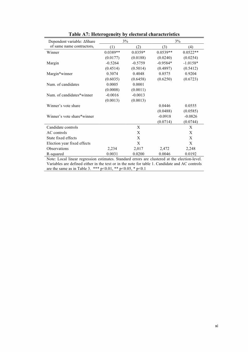
xi

Table A7: Heterogeneity by electoral characteristics Dependent variable: ΔShare of same name contractorst

3% 3% (1) (2) (3) (4)

Winner 0.0389** 0.0359* 0.0539** 0.0522**

(0.0177) (0.0188) (0.0240) (0.0254)

Margin -0.5264 -0.5759 -0.9584* -1.0158*

(0.4514) (0.5014) (0.4897) (0.5412)

Margin*winner 0.3074 0.4048 0.8575 0.9204

(0.6035) (0.6458) (0.6250) (0.6723) Num. of candidates 0.0005 0.0001

(0.0008) (0.0011) Num. of candidates*winner -0.0016 -0.0013

(0.0013) (0.0013)

Winner’s vote share

0.0446 0.0555

(0.0488) (0.0585)

Winner’s vote share*winner

-0.0918 -0.0826 (0.0714) (0.0744) Candidate controls

X

X

AC controls

X

X State fixed effects

X

X

Election year fixed effects

X

X Observations 2,234 2,017 2,472 2,248 R-squared 0.0031 0.0200 0.0046 0.0192 Note: Local linear regression estimates. Standard errors are clustered at the election-level. Variables are defined either in the text or in the note for table 1. Candidate and AC controls are the same as in Table 3. *** p<0.01, ** p<0.05, * p<0.1

xii

Table A8: Parametric regression discontinuity estimated on full sample Dependent variable:

ΔSharet Linear Quadratic Polynomials Cubic Polynomials

(1) (2) (3) (4) (5) (6) Winner 0.0094* 0.0099* 0.0138** 0.0137** 0.0190** 0.0184**

(0.0052) (0.0054) (0.0062) (0.0065) (0.0075) (0.0079)

Margin -0.0001 0.0114 -0.0226 -0.0028 -0.1004 -0.1102

(0.0299) (0.0337) (0.0609) (0.0664) (0.1209) (0.1295)

Margin*Winner -0.0059 -0.0353 -0.0740 -0.1037 -0.1247 -0.0749

(0.0414) (0.0445) (0.0870) (0.0945) (0.1604) (0.1722)

Margin^2

-0.0764 -0.0473 -0.6165 -0.7856

(0.1540) (0.1635) (0.6727) (0.7226)

Margin*Winner ^2

0.3834 0.3219 1.8161* 1.6014

(0.2689) (0.2634) (1.0541) (1.0722)

Margin ^3

-0.8224 -1.1115

(0.8418) (0.9053)

Margin*Winner ^3

-0.5365 0.2950

(1.0901) (1.1569)

Constituency-level controls X X X Candidate-level controls X X X State fixed effects X X X Election year fixed effects X X X N 8,116 7,290 8,116 7,290 8,116 7,290 Note: Estimated by OLS. Standard errors are clustered at the election-level. Variables are defined either in the text or in the note for table 1. The candidate and constituency level controls in columns 2, 4, 6 and 8 are the same as in column (2) of Table 3. These controls and state and election year fixed effects are not reported. All regressions include a constant. *** p<0.01, ** p<0.05, * p<0.1

xiii

Table A9: 2nd vs 3rd Placebo Tests Dependent variable: ΔShare of same name contractorst

All 2nd vs 3rd with margin < 3%

2nd vs 3rd where margin between 1st and 2nd <3%

2nd vs 3rd where both margins <3%

(1) (2) (3) (4) (5) (6) 2nd place -0.0282 -0.0132 0.0046 0.0038 0.0094 0.0463

(0.0176) (0.0190) (0.0122) (0.0138) (0.0318) (0.0368)

Margin (2nd vs 3rd) 1.0832 0.1563 -0.0257 0.0625 0.5122 -1.4668

(0.8269) (0.8767) (0.0394) (0.0573) (1.6560) (2.0495)

Margin*2nd place -1.2061 -0.2548 0.0023 -0.1978** -1.4159 0.3412 (1.0470) (1.1582) (0.0505) (0.0839) (1.9071) (2.3849)

Candidate controls X X X AC controls X X X State fixed effects X X X Election year fixed effects X X X N 1,216 1,002 2,368 1,911 456 371 Note: the regressions in this table are equivalent to those in Table 3, except that these compare 2nd placed candidates to 3rd placed candidates. In columns (1) and (2) the sample is restricted to candidates whose difference in vote shares was smaller than 3% (as in the main specification). Columns (3) and (4) compare 2nd and 3rd placed candidates in the elections that make up the sample for the main specification. The sample for columns (5) and (6) is the intersection of the previous two, including candidates from elections where both the gap between 1st and 2nd and between 2nd and 3rd was smaller than 3%. Standard errors are clustered at the election level. All regressions include a constant. *** p<0.01, ** p<0.05, * p<0.1

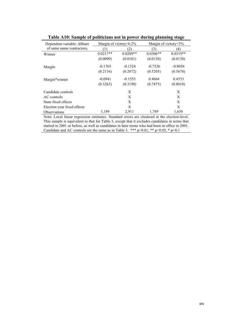
xiv

Table A10: Sample of politicians not in power during planning stage

Dependent variable: ΔShare of same name contractorst

Margin of victory<6.2% Margin of victory<3% (1) (2) (3) (4)

Winner 0.0217** 0.0209** 0.0306** 0.0319**

(0.0099) (0.0101) (0.0130) (0.0138)

Margin -0.1765 -0.1324 -0.7526 -0.8056

(0.2116) (0.2072) (0.5205) (0.5678)

Margin*winner -0.0941 -0.1553 0.4664 0.4533

(0.3263) (0.3198) (0.7475) (0.8018)

Candidate controls

X

X AC controls

X

X

State fixed effects

X

X Election year fixed effects

X

X

Observations 3,189 2,911 1,789 1,630 Note: Local linear regression estimates. Standard errors are clustered at the election-level. This sample is equivalent to that for Table 3, except that it excludes candidates in terms that started in 2001 or before, as well as candidates in later terms who had been in office in 2001. Candidate and AC controls are the same as in Table 3. *** p<0.01, ** p<0.05, * p<0.1

xv

Table A11: Continuity test for road level local linear regression at 3% bandwidth

Observations Winner P value

Panel A: Local Geography Altitude 1,470 10.3736 (0.8787) Ruggedness 1,470 0.1615 (0.1995) Forest cover 1,470 0.0280** (0.0125) Distance to nearest town 1,470 -1.9768 (0.2988) Panel B: Village Demographics Total population 1,470 303.22 (0.3392) Number of households 1,470 49.9927 (0.3728) Village area 1,470 188.54 (0.4854) Sex ratio 1,468 -0.0000 (0.9992) Population under 6 1,470 -0.0016 (0.7036) SC share 1,470 0.0223 (0.1999) ST share 1,470 0.0268 (0.2403) Panel C: Village Socioeconomic Characteristics Literacy 1,071 -0.0168 (0.5513) Employment 1,071 0.0084 (0.5837) Male employment 1,071 0.0154 (0.1211) Female employment 1,071 0.0105 (0.6901) Irrigated area under cultivation 1,387 -0.0260 (0.5689) Unirrigated area under cultivation 1,404 0.0495 (0.2063) Drinking water 1,470 0.0015 (0.5637) Power supply 1,470 -0.0368 (0.4735) Phone connections 1,470 -7.5092 (0.2526) Primary school 1,470 0.1500 (0.4988) Medical facility 1,470 0.0702 (0.2655) Health centre 1,470 0.0236 (0.1879) Post office 1,470 0.0419 (0.4602) Bank 1,470 0.0064 (0.8450) Road connectivity in 2001 1,470 0.0005 (0.9933) Mud road 1,375 0.0774 (0.1425) Foot path 1,281 -0.0700 (0.1848) Panel D: Pre-determined Road Characteristics Length of road 1,470 0.1346 (0.2357) Bridge 1,470 -0.0219* (0.0654) Note: Coefficients are estimated by regressing the row variables on winner, the vote margin, and the vote margin interacted with winner in OLS regressions, including state and year fixed effects. Standard errors are clustered at the contractor level. Where a road passes through multiple villages, the road level variable is an average of all villages on that road. *** p<0.01, ** p<0.05, * p<0.1

xvi

Table A12a: Road-level RD sample at multiple bandwidths – missing roads Panel A

Dependent variable: Missing all-weather road Missing any road

Margin of victory: <5% Opt. BW <2.48% <2.5% <5% Opt. BW

<4.4% <2.5%

(1) (2) (3) (4) (5) (6) Same name as MLA 0.0849 0.300*** 0.26*** 0.0822* 0.0913* 0.1580**

(0.0748) (0.0991) (0.0960) (0.0418) (0.0471) (0.0721)

Margin 3.2279 -7.1166 -5.4180 0.1886 -1.0443 -3.7428* (1.9719) (4.7207) (4.7713) (0.9401) (1.0967) (2.2274)

Margin*same name as MLA -5.5556* -4.0300 -5.6604 -2.6142* -1.0541 -0.6751 (3.1955) (7.3736) (7.3804) (1.5557) (1.7138) (4.2556)

Road-level controls X X X X X X State fixed effects X X X X X X Agreement year FE X X X X X X N 829 456 464 829 757 464 Note: Standard errors clustered at the contractor level to account for intra-contractor correlation of the error term at the road level. Road-level controls are equivalent to the full set of controls used in columns 2 and 4 of Table 4. The optimal bandwidths of 2.5% (for missing all-weather roads), and 4.4% (for missing any roads), are derived from the optimal bandwidth choice rule of Imbens and Kalyanaraman (2011). All regressions include a constant. *** p<0.01, ** p<0.05, * p<0.1

xvii

Table A12b: Road-level regression discontinuity - estimates for quality Panel B

Dependent variable: Log of (sanctioned cost/km) Days overrun Ratio: actual cost to sanctioned cost Failed inspection

Margin of victory: <5% <2.7% <2.5% <5% <3% <2.5% <5% <3.5% <2.5% <5% <4.3% <2.5% (1) (2) (3) (4) (5) (6) (7) (8) (9) (10) (11) (12) Same name as MLA 0.069* 0.117** 0.116** -108.7 -78.1 -134.1 -0.055 -0.057 -0.040 0.150* 0.162* 0.137

(0.037) (0.048) (0.050) (70.6) (95.1) (110.6) (0.035) (0.044) (0.055) (0.078) (0.083) (0.109)

Margin -1.578 -7.331*** -7.641*** 127.2 -1,176.1 883.3 1.180 2.733 2.216 -1.995 -1.894 -1.522 (1.029) (2.532) (2.772) (1,913.5) (4,548.6) (4,693.4) (1.226) (2.043) (3.204) (2.285) (3.018) (5.645)

Margin*same name as MLA 1.930 8.533** 8.972** 1,663.0 1,784.4 3,458.7 -0.591 -3.488 -3.577 -3.663 -4.272 -4.204 (1.456) (3.479) (3.713) (2,759.9) (5,551.0) (6,163.0) (1.539) (2.433) (4.063) (3.109) (3.985) (7.081)

Road level controls X X X X X X X X X X X X State fixed effects X X X X X X X X X X X X Agreement year FE X X X X X X X X X X X X N 2,124 1,340 1,234 1,386 970 794 1,671 1,334 960 719 660 407 Note: Standard errors clustered at the contractor level to account for intra-contractor correlation of the error term at the road level. All regressions include the full set of road level controls from cols 2, 4, 6, and 8 in Table 5. The optimal bandwidths of 2.7% (for cost/km), 3% (for days overrun), 3.5% (for cost overruns), and 4.3% (for failed inspections) are derived from the optimal bandwidth choice rule of Imbens and Kalyanaraman (2011). All regressions include a constant. *** p<0.01, ** p<0.05, * p<0.1

xviii

Table A13: Robustness to outliers in road level data Dependent Variable: Log of (sanctioned cost/km) Days Overrun Actual cost/sanctioned cost

Margin of Victory <3% Margin of Victory <3% Margin of Victory <3%

Full sample Dropping

bottom 1% and top 1%

Dropping bottom 5% and top 5%

Full sample Dropping

bottom 1% and top 1%

Dropping bottom 5% and top 5%

Full sample Dropping

bottom 1% and top 1%

Dropping bottom 5% and top 5%

(1) (2) (3) (4) (5) (6) (7) (8) (9)

Same name as MLA 0.116** 0.113** 0.089* -88.9 -44.3 -26.2 -0.052 -0.002 0.008

(0.050) (0.050) (0.050) (91.6) (73.0) (67.2) (0.053) (0.025) (0.017)

Margin -7.681*** -7.582*** -5.278** -472.1 377.6 -300.0 1.870 -1.025 -2.133**

(2.576) (2.574) (2.464) (4,423.1) (3,696.2) (3,337.5) (2.713) (1.184) (0.858)

Margin*same name as MLA

10.419*** 10.590*** 7.819** 1,076.6 -2,359.6 -320.3 -2.177 0.992 3.104***

(3.342) (3.354) (3.236) (5,546.3) (4,799.7) (4,164.2) (2.998) (1.433) (1.045)

Road-level controls X X X X X X X X XState fixed effects X X X X X X X X XYear fixed effects X X X X X X X X X N 1,470 1,449 1,327 970 956 908 1,161 1,143 1,056 Note: Standard errors clustered at the contractor level to account for intra-contractor correlation of the error term at the road level. All regressions include the following set of road-level controls: ln(length) (to account for non-linear relationship between cost and distance), whether the constituency is a reserved seat, the mean population of habitations on the road, the mean population share of Scheduled Castes and Scheduled Tribes of habitations on the road, and the mean connectivity of those habitations in 2001. *** p<0.01, ** p<0.05, * p<0.1

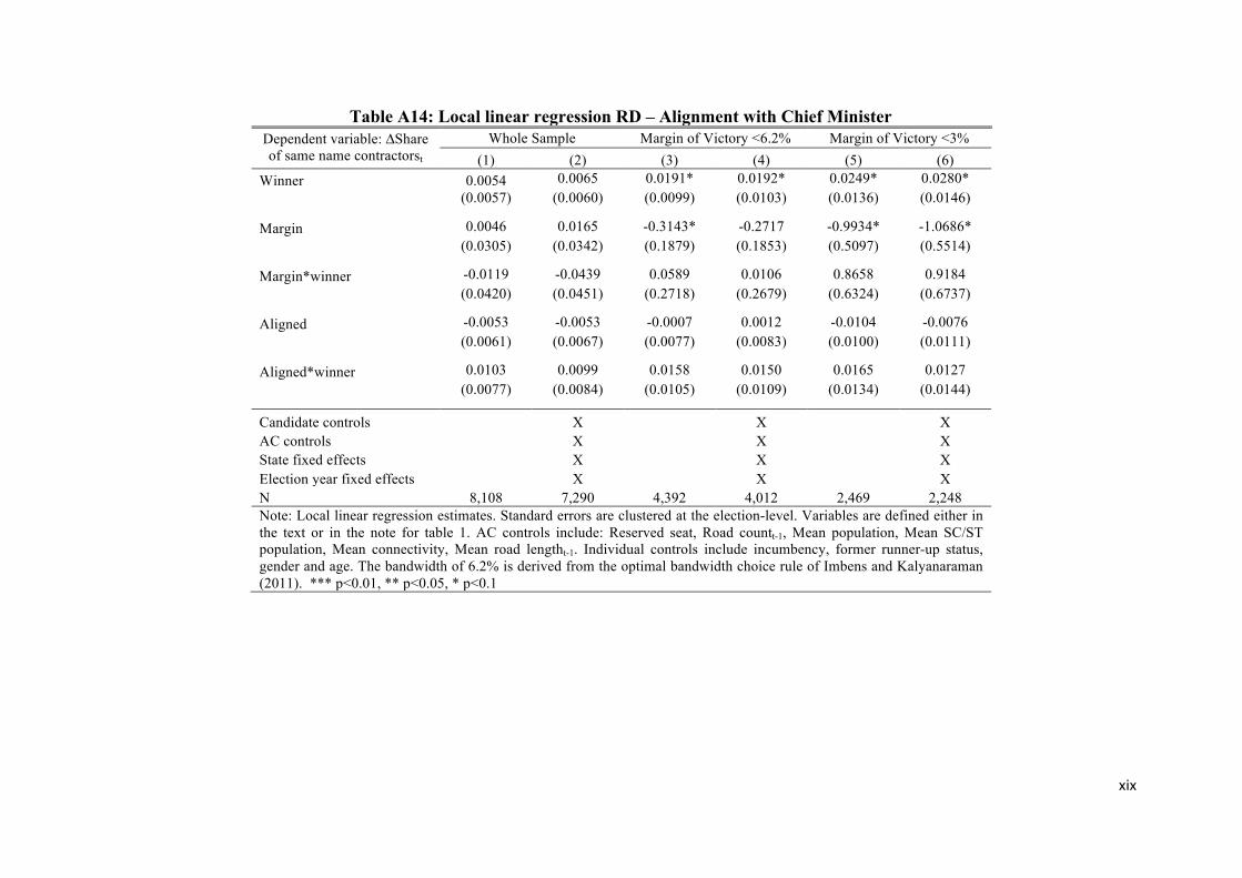
xix

Table A14: Local linear regression RD – Alignment with Chief Minister Dependent variable: ΔShare of same name contractorst

Whole Sample Margin of Victory <6.2% Margin of Victory <3% (1) (2) (3) (4) (5) (6)

Winner 0.0054 0.0065 0.0191* 0.0192* 0.0249* 0.0280*

(0.0057) (0.0060) (0.0099) (0.0103) (0.0136) (0.0146)

Margin 0.0046 0.0165 -0.3143* -0.2717 -0.9934* -1.0686*

(0.0305) (0.0342) (0.1879) (0.1853) (0.5097) (0.5514)

Margin*winner -0.0119 -0.0439 0.0589 0.0106 0.8658 0.9184 (0.0420) (0.0451) (0.2718) (0.2679) (0.6324) (0.6737)

Aligned -0.0053 -0.0053 -0.0007 0.0012 -0.0104 -0.0076 (0.0061) (0.0067) (0.0077) (0.0083) (0.0100) (0.0111)

Aligned*winner 0.0103 0.0099 0.0158 0.0150 0.0165 0.0127 (0.0077) (0.0084) (0.0105) (0.0109) (0.0134) (0.0144)

Candidate controls X X X AC controls

X

X

X

State fixed effects X X X Election year fixed effects X X X N 8,108 7,290 4,392 4,012 2,469 2,248 Note: Local linear regression estimates. Standard errors are clustered at the election-level. Variables are defined either in the text or in the note for table 1. AC controls include: Reserved seat, Road countt-1, Mean population, Mean SC/ST population, Mean connectivity, Mean road lengtht-1. Individual controls include incumbency, former runner-up status, gender and age. The bandwidth of 6.2% is derived from the optimal bandwidth choice rule of Imbens and Kalyanaraman (2011). *** p<0.01, ** p<0.05, * p<0.1

xx

Table A15: Robustness checks for promotion screening results

Dependent variable: ΔShare of same name contractorst

Margin of victory <6.2% Margin of victory <3% Margin of victory <6.2% Margin of victory <3% (1) (2) (3) (4) (5) (6) (7) (8)

Winner 0.0342** 0.0332* 0.0404** 0.0403** 0.0254*** 0.0225** 0.0254*** 0.0225**

(0.0165) (0.0182) (0.0177) (0.0192) (0.0096) (0.0101) (0.0096) (0.0101)

DC in promotion year 0.0053 0.0066 0.0207* 0.0258** 0.0125 0.0161* 0.0125 0.0161* (0.0080) (0.0091) (0.0114) (0.0126) (0.0088) (0.0097) (0.0088) (0.0097) DC in promotion year*winner -0.0274* -0.0273* -0.0308 -0.0420** -0.0342** -0.0342** -0.0342** -0.0342** (0.0140) (0.0148) (0.0187) (0.0205) (0.0144) (0.0153) (0.0144) (0.0153) Years of service 0.0011 0.0014 0.0008 0.0001 (0.0009) (0.0011) (0.0012) (0.0014) Years of service *winner -0.0012 -0.0013 -0.0010 -0.0006 (0.0015) (0.0017) (0.0018) (0.0020) Promotion year – 2 0.0031 0.0013 0.0031 0.0013 (0.0076) (0.0084) (0.0076) (0.0084) Promotion year – 2*winner 0.0011 0.0029 0.0011 0.0029

(0.0129) (0.0140) (0.0129) (0.0140) Promotion year – 1 0.0153 0.0207* 0.0153 0.0207* (0.0097) (0.0110) (0.0097) (0.0110) Promotion year – 1*winner -0.0277* -0.0252 -0.0277* -0.0252

(0.0146) (0.0159) (0.0146) (0.0159) Promotion year + 1 0.0023 0.0059 0.0023 0.0059 (0.0103) (0.0118) (0.0103) (0.0118) Promotion year + 1*winner -0.0021 -0.0018 -0.0021 -0.0018

(0.0143) (0.0159) (0.0143) (0.0159) Promotion year + 2

-0.0056 -0.0105 -0.0056 -0.0105

(0.0145) (0.0169) (0.0145) (0.0169) Promotion year + 2*winner

0.0327 0.0264 0.0327 0.0264

(0.0247) (0.0266) (0.0247) (0.0266) Candidate and AC Controls X X X X State and election year FE N 7,336 6,607 4,144 3,730 7,358 6,629 7,358 6,629 Note: Local linear regression estimates. Standard errors are clustered at the district-level. All regressions control for margin and its interaction with winner. Candidate and AC controls and fixed effects as in Table 6. *** p<0.01, ** p<0.05, * p<0.1

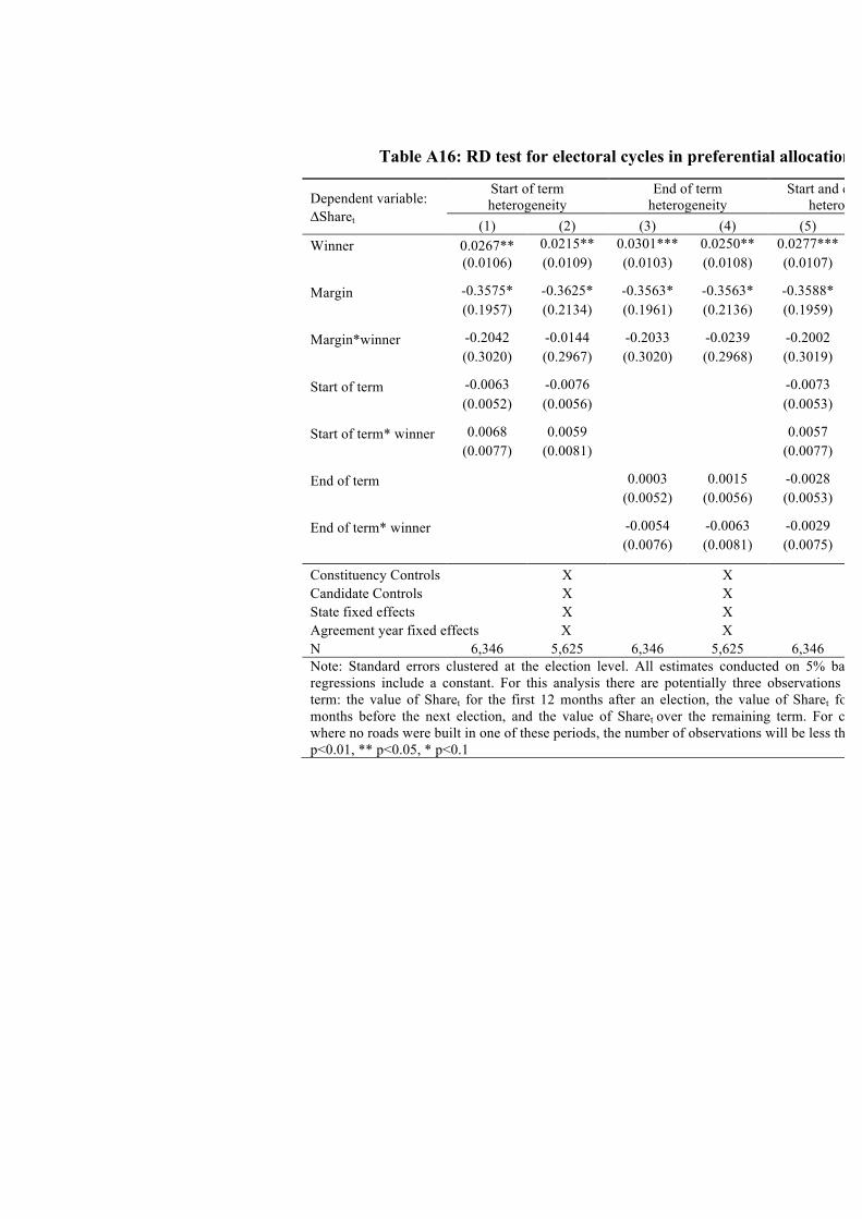
xxi

Table A16: RD test for electoral cycles in preferential allocation

Dependent variable: ΔSharet

Start of term heterogeneity

End of term heterogeneity

Start and end of term heterogeneity

(1) (2) (3) (4) (5) (6) Winner 0.0267** 0.0215** 0.0301*** 0.0250** 0.0277*** 0.0232**

(0.0106) (0.0109) (0.0103) (0.0108) (0.0107) (0.0112)

Margin -0.3575* -0.3625* -0.3563* -0.3563* -0.3588* -0.3608* (0.1957) (0.2134) (0.1961) (0.2136) (0.1959) (0.2135)

Margin*winner -0.2042 -0.0144 -0.2033 -0.0239 -0.2002 -0.0160 (0.3020) (0.2967) (0.3020) (0.2968) (0.3019) (0.2969)

Start of term -0.0063 -0.0076

-0.0073 -0.0082

(0.0052) (0.0056)

(0.0053) (0.0058)

Start of term* winner 0.0068 0.0059

0.0057 0.0043

(0.0077) (0.0081)

(0.0077) (0.0081)

End of term

0.0003 0.0015 -0.0028 -0.0020

(0.0052) (0.0056) (0.0053) (0.0057)

End of term* winner

-0.0054 -0.0063 -0.0029 -0.0045

(0.0076) (0.0081) (0.0075) (0.0081)

Constituency Controls X X X Candidate Controls X X X State fixed effects X X X Agreement year fixed effects X X X N 6,346 5,625 6,346 5,625 6,346 5,625 Note: Standard errors clustered at the election level. All estimates conducted on 5% bandwidth. All regressions include a constant. For this analysis there are potentially three observations per electoral term: the value of Sharet for the first 12 months after an election, the value of Sharet for the last 12 months before the next election, and the value of Sharet over the remaining term. For constituencies where no roads were built in one of these periods, the number of observations will be less than three. *** p<0.01, ** p<0.05, * p<0.1

xxii

Table A17: RD test for electoral cycles in cost

Dependent variable: Log of (sanctioned cost/km)

Start of term heterogeneity

End of term heterogeneity

Start and end of term heterogeneity

(1) (2) (3) Same name as MLA 0.1414*** 0.1522*** 0.1652***

(0.0530) (0.0535) (0.0553)

Margin -7.9813*** -8.1813*** -7.7047*** (2.6897) (2.7732) (2.7220)

Margin*same name as MLA 9.1694** 9.1362** 8.7095** (3.6056) (3.6984) (3.6404)

Start of term 0.1365***

0.1475*** (0.0418)

(0.0445)

Start of term* same name as MLA

-0.0993*

-0.1193** (0.0556)

(0.0562)

End of term

0.0300 0.0572

(0.0597) (0.0611)

End of term* same name as MLA

-0.1249** -0.1455**

(0.0592) (0.0595)

Road level controls X X X State fixed effects X Agreement year FE X N 1,340 1,340 1,340 Note: Standard errors clustered at the contractor level. All estimates conducted on optimal bandwidth of 2.7% derived from the optimal bandwidth choice rule of Imbens and Kalyanaraman (2011) . The set of road-level controls is the same as in Table 4 and Table 5. All regressions include a constant. *** p<0.01, ** p<0.05, * p<0.1

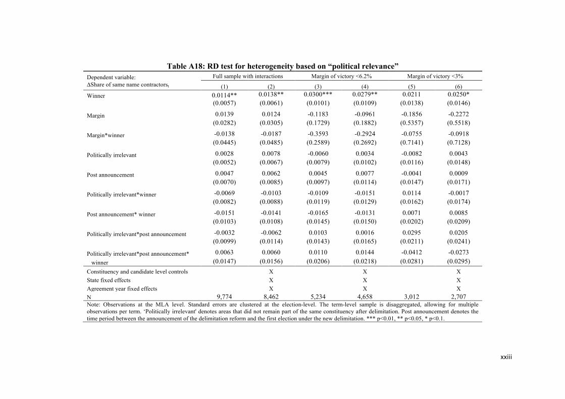
xxiii

Table A18: RD test for heterogeneity based on “political relevance”

Dependent variable: ΔShare of same name contractorst

Full sample with interactions Margin of victory <6.2% Margin of victory <3%

(1) (2) (3) (4) (5) (6) Winner 0.0114** 0.0138** 0.0300*** 0.0279** 0.0211 0.0250*

(0.0057) (0.0061) (0.0101) (0.0109) (0.0138) (0.0146)

Margin 0.0139 0.0124 -0.1183 -0.0961 -0.1856 -0.2272 (0.0282) (0.0305) (0.1729) (0.1882) (0.5357) (0.5518)

Margin*winner -0.0138 -0.0187 -0.3593 -0.2924 -0.0755 -0.0918 (0.0445) (0.0485) (0.2589) (0.2692) (0.7141) (0.7128)

Politically irrelevant 0.0028 0.0078 -0.0060 0.0034 -0.0082 0.0043

(0.0052) (0.0067) (0.0079) (0.0102) (0.0116) (0.0148)

Post announcement 0.0047 0.0062 0.0045 0.0077 -0.0041 0.0009

(0.0070) (0.0085) (0.0097) (0.0114) (0.0147) (0.0171)

Politically irrelevant*winner -0.0069 -0.0103 -0.0109 -0.0151 0.0114 -0.0017

(0.0082) (0.0088) (0.0119) (0.0129) (0.0162) (0.0174)

Post announcement* winner -0.0151 -0.0141 -0.0165 -0.0131 0.0071 0.0085

(0.0103) (0.0108) (0.0145) (0.0150) (0.0202) (0.0209)

Politically irrelevant*post announcement -0.0032 -0.0062 0.0103 0.0016 0.0295 0.0205

(0.0099) (0.0114) (0.0143) (0.0165) (0.0211) (0.0241)

Politically irrelevant*post announcement* 0.0063 0.0060 0.0110 0.0144 -0.0412 -0.0273 winner (0.0147) (0.0156) (0.0206) (0.0218) (0.0281) (0.0295) Constituency and candidate level controls X X X State fixed effects

X X X

Agreement year fixed effects X X X N 9,774 8,462 5,234 4,658 3,012 2,707 Note: Observations at the MLA level. Standard errors are clustered at the election-level. The term-level sample is disaggregated, allowing for multiple observations per term. ‘Politically irrelevant' denotes areas that did not remain part of the same constituency after delimitation. Post announcement denotes the time period between the announcement of the delimitation reform and the first election under the new delimitation. *** p<0.01, ** p<0.05, * p<0.1.

xxiv

Table A19: Within-constituency heterogeneity All constituencies All constituencies Unreserved constituencies

Dependent variable: ΔShare of same name contractorst

Margin of Victory <3% Margin of Victory <3% Margin of Victory <3% (1) (2) (3) (4) (5) (6)

Winner 0.0336** 0.0327** 0.0330*** 0.0344*** 0.0451*** 0.0465***

(0.0133) (0.0143) (0.0124) (0.0130) (0.0165) (0.0173)

Margin -0.587 -0.659 -0.969* -1.063** -1.678** -1.826**

(0.491) (0.536) (0.495) (0.530) (0.661) (0.714)

Margin*winner -0.116 0.0177 0.576 0.679 1.035 1.190 (0.625) (0.666) (0.632) (0.660) (0.842) (0.890)

Panchayat HQ villages 0.00380 0.00503 (0.00780) (0.00888)

Panchayat HQ villages*winner -0.00648 -0.00626 (0.0120) (0.0129)

SC/ST majority villages 0.000904 0.00232 -0.00183 -0.00256 (0.00894) (0.0104) (0.0134) (0.0152)

SC/ST maj. villages*winner -0.00004 0.00346 0.0170 0.0214 (0.0126) (0.0134) (0.0186) (0.0197)

Candidate controls

X

X

X AC controls State fixed effects X X X Election year fixed effects X X X N 3,252 3,001 3,304 3,006 2,350 2,143 Note: Local linear regression estimates. Standard errors are clustered at the election-level. Constituencies are split: villages with panchayat HQs vs all other villages in columns (1) and (2); villages that are majority SC and ST vs all other villages in columns (3) to (6). Columns (5) and (6) restrict the sample to constituencies not reserved for SC or ST politicians. *** p<0.01, ** p<0.05, * p<0.1

xxv

Table A20: Alignment and party seat share

Dependent variable: ΔShare of same name contractorst

3% 3% (1) (2) (3) (4)

Winner 0.0306** 0.0306* 0.0269* 0.0296*

(0.0153) (0.0164) (0.0158) (0.0171)

Margin -1.0131** -1.0758* -0.9752* -1.0554*

(0.5058) (0.5497) (0.5151) (0.5565)

Margin*winner 0.8613 0.9424 0.8702 0.9165

(0.6342) (0.6733) (0.6388) (0.6786) Party seat share -0.0101 -0.0071 -0.0038 0.0029

(0.0173) (0.0203) (0.0256) (0.0332)

Party seat share*winner 0.0043 0.0056 -0.0119 -0.0091

(0.0264) (0.0273) (0.0356) (0.0381)

Aligned -0.0387 -0.0196 (0.0379) (0.0439)

Aligned*winner 0.0686 0.0547 (0.0523) (0.0557)

Party seat share*aligned

0.0571 0.0214

(0.0680) (0.0840)

Party seat share*aligned*winner

-0.0924 -0.0748

(0.0961) (0.1002)

Candidate controls

X

X AC controls

X

X

State fixed effects

X

X Election year fixed effects

X

X

Observations 2,472 2,248 2,469 2,248 Note: Local linear regression estimates. Standard errors are clustered at the election-level. Party seat share is the number of seats the candidate’s party won in the election divided by the number of seats in the state. Variables are defined either in the text or in the note for table 1. Candidate and AC controls are the same as in Table 3. *** p<0.01, ** p<0.05, * p<0.1

xxvi

Table A21: E-Procurement Dependent variable: ΔShare of same name contractorst

Whole Sample Margin of Victory <6.2% Margin of Victory <3% (1) (2) (3) (4) (5) (6)

Winner 0.0092 0.0113* 0.0278*** 0.0273** 0.0407*** 0.0428**

(0.0060) (0.0067) (0.0107) (0.0117) (0.0153) (0.0173)

Margin -0.0274 -0.0073 -0.4330** -0.5064** -1.1253* -1.4149**

(0.0266) (0.0318) (0.2043) (0.2121) (0.5810) (0.6507)

Margin*winner 0.0420 -0.0235 0.1885 0.3052 0.8833 1.2506 (0.0407) (0.0461) (0.2684) (0.2833) (0.7418) (0.8296)

E-procurement -0.0052 -0.0073 -0.0015 -0.0114 -0.0033 -0.0049 (0.0039) (0.0059) (0.0056) (0.0090) (0.0078) (0.0121)

E-procurement*winner 0.0033 0.0038 0.0032 0.0070 -0.0053 -0.0030 (0.0058) (0.0064) (0.0086) (0.0093) (0.0114) (0.0127)

AC controls

X

X

X Candidate controls X X X State fixed effects X X X Election year fixed effects X X X N 9,990 8,612 5,324 4,665 3,012 2,625 Note: Local linear regression estimates. Standard errors are clustered at the election-level. Variables are defined either in the text or in the note for table 1. AC controls include: Reserved seat, Road countt-1, Mean population, Mean SC/ST population, Mean connectivity, Mean road lengtht-1. Candidate controls: age, gender, incumbency, former-runner-up status*** p<0.01, ** p<0.05, * p<0.1