LOW SALINITY WATER FLOODING SIMULATION STUDY

by

LOW JUN LEON, 12638

SUPERVISOR: ISKANDAR B DZULKARNAIN

DISSERTATION

Submitted to the Petroleum Engineering Programme

Universiti Teknologi PETRONAS

in partial fulfilment of the requirements

for the Bachelor of Engineering (Hons) Degree in Petroleum Engineering

Universiti Teknologi Petronas

Bandar Seri Iskandar

31750 Tronoh

Perak Darul Ridzuan

May 2013

i

CERTIFICATION OF APPROVAL

LOW SALINITY WATER FLOODING SIMULATION STUDY

by

LOW JUN LEON, 12638

A project dissertation submitted to the Petroleum Engineering Programme

Universiti Teknologi PETRONAS

in partial fulfilment of the requirements

for the Bachelor of Engineering (Hons) Degree in Petroleum Engineering

Aprroved by,

______________________________

(ISKANDAR B DZULKARNAIN)

Universiti Teknologi Petronas

Bandar Seri Iskandar

31750 Tronoh

Perak Darul Ridzuan

August 2013

ii

CERTIFICATION OF ORIGINALITY

This is to certify that I am responsible for the work submitted in this project, that the

original work is my own except as specified in the references and acknowledgements,

and that the original work contained herein have not been undertaken or done by

unspecified sources or persons.

________________

LOW JUN LEON

iii

ACKNOWLEDGMENTS

First of all, I would like to express my greatest gratitude to my campus,

Universiti Teknologi PETRONAS (UTP) for providing a conducive learning

environment in completing my Final Year Project. This project has allowed me to

have a great exposure on the right methodology to carry out a research. Moreover, I

have gained better understanding about prospect of Enhanced Oil Recovery(EOR)

mechanism, especially on low salinity water flooding.

Many thanks go to my supervisor, Mr.Iskandar B Dzulkarnain. Without his

guidance and supervision throughout these two semesters, this project will not be

succeeded. His crucial contribution has kept my research work on the right track.

Lastly, I would like to say thank you to my parents and friends who morally

supported and encouraged me during conducting this study.

iv

ABSTRACT

Low salinity water flooding(LSWF) is a recent enhanced oil recovery (EOR)

method which is applied by injecting water with a lower salinity than initial connate

water. Although a lot of laboratory experiments and tests have shown LSWF’s

potential in EOR, There have not been done many modelling studies on this field.

Moreover, there is lack of economic analysis to justify the application of LSWF for

most of the simulation studies. Several hypotheses have proposed as LSWF

mechanisms, namely electrical double layer effect, pH effect, fines migration and

multicomponent ion exchange (MIE). However, there is still no definite theory that

supports LSWF effects. Thus, the main objective of this research is to evaluate the

effects of salinity in LSWF on oil recovery.

In this study, effects of salinity in LSWF are investigated through simulations

of a 3 dimensional synthetic reservoir model by ECLIPSE 100 software. The model

is lateral heterogeneous with only oil and water phase. Moreover, only one type of

salt is assumed to be present in the water. There are 2 base cases in the first phase of

study. The first base case uses high salinity(HS) water flooding technique by

injecting 35000ppm of brine from the starting to the end of production, totally 10

years or 3650 days. The other case uses low salinity water flooding technique by

injecting 1000ppm of brine continuously for the same production life, in order to

compare the effect of salinity with the HS base case. Large wettability sensitivity

was observed, showing that oil/water relative permeability and saturation are the

main variables during simulations when BRINE option is activated. Findings

obtained after injection of brines with different salinities indicated oil recovery

improves with a decrease in salinity of the injected brines. Then, the second phase of

the study will be comparing the oil recovery by alternating the LS and HS injection

days. HS will be the first phase of injection followed by LS. Different cases will be

simulated in this phase and evaluated through economic analysis. The best LSWF

case will be selected after considering its economic feasibility.

v

TABLE OF CONTENTS

CERTIFICATION OF APPROVAL ............................................................................ i

CERTIFICATION OF ORIGINALITY ...................................................................... ii

ACKNOWLEDGMENTS ......................................................................................... iii

ABSTRACT ................................................................................................................ iv

LIST OF FIGURES ................................................................................................... vii

LIST OF TABLES ................................................................................................... viii

CHAPTER 1 ................................................................................................................ 1

INTRODUCTION ....................................................................................................... 1

1.1 Background of Study .......................................................................................... 1

1.2 Problem Statement ............................................................................................. 2

1.2.1 Problem Identification ................................................................................. 2

1.2.2 Significance of Project ................................................................................. 2

1.3 Objectives ........................................................................................................... 2

1.4 Scope of Study .................................................................................................... 3

1.5 Relevancy of Project .......................................................................................... 3

1.6 Feasibility of the Project within the Scope and Time Frame ............................. 3

CHAPTER 2 ................................................................................................................ 4

LITERATURE REVIEW............................................................................................. 4

2.1 Enhanced Oil Recovery (EOR) .......................................................................... 4

2.2 Low Salinity Water Flooding ............................................................................. 5

2.3 Conditions for Low Salinity Effects ................................................................... 6

2.4 Proposed Mechanisms for LSWF ....................................................................... 7

2.4.1 Electrical Double Layer Effects ................................................................... 7

2.4.2 pH Effect ...................................................................................................... 9

2.4.3 Fines Migration .......................................................................................... 10

2.4.4 Multicomponent Ion Exchange (MIE) ....................................................... 12

2.5 Low Salinity Water Flooding Model ................................................................ 14

2.6 Summary .......................................................................................................... 15

CHAPTER 3 .............................................................................................................. 16

METHODOLOGY ..................................................................................................... 16

3.1 Research Methodology ..................................................................................... 16

vi

3.2 Project Activities .............................................................................................. 17

3.3 Gantt Chart and Key Milestones ...................................................................... 18

3.4 Low Salinity Water Flooding (LSWF): Options in ECLIPSE 100 .................. 20

3.5 Synthetic Model and Properties ....................................................................... 22

3.6 Simulation Study Work Flow ........................................................................... 26

3.7 Tools Required ................................................................................................. 27

CHAPTER 4 .............................................................................................................. 28

RESULTS AND DISCUSSIONS .............................................................................. 28

4.1 Effect of LSWF in Secondary Recovery Phase ................................................ 28

4.1.1 Effect of the Salinity on Recovery Factor ................................................. 28

4.1.2 Effect of salinity on Oil Production Rate and Cumulative Oil Production 28

4.1.3 Comparison of Salt Production Rate and Salt Production Concentration . 30

4.1.4 Summary of LSWF Simulation Results in Secondary Recovery Phase .... 30

4.2 Effect of LSWF in Tertiary Recovery Phase .................................................... 32

4.2.2 Effect of Salinity Concentration in Tertiary Recovery Phase.................... 34

4.2.3 Summary of LSWF Simulation Results in Tertiary Recovery Phase ........ 42

4.3 Sensitivity Study of LSWF Economics ............................................................ 43

4.3.1 Economic Evaluation ................................................................................. 43

4.3.2 Economic Simulation Results and Analysis .............................................. 46

4.3.3 Summary of Economic Simulation Results and Analysis ......................... 48

CHAPTER 5 .............................................................................................................. 50

CONCLUSIONS AND RECOMMENDATIONS .................................................... 50

5.1 Conclusions ...................................................................................................... 50

5.2 Recommendations for Future Work ................................................................. 51

REFERENCES ........................................................................................................... 52

APPENDICES ........................................................................................................... 55

APPENDIX A ........................................................................................................ 55

APPENDIX B ......................................................................................................... 56

APPENDIX C ......................................................................................................... 60

APPENDIX D ........................................................................................................ 64

vii

LIST OF FIGURES

Figure No. Descriptions

1 How double layer worked

2 Detachment of clay particles and mobilization of oil

3 Attraction between clay surface and crude oil by divalent cations

4 Synthetic model with well placements and initial salt concentration

5 Synthetic model showing permeability in Z direction

6 Synthetic model showing permeability in X direction

7 ECLIPSE simulation software launcher 2009.1

8 Comparison of oil recovery factor

9 Comparison of oil cumulative production (FOPT) and oil production

rate (FOPR)

10 Comparison of salt production concentration

11 Comparison of salt production rate

12 Effect of Timing of LS injection in Secondary Recovery Phase

13 Effect of Timing of LS injection on Field Oil Production Rate

(FOPR)

14 Effect of salinity on recovery factor in tertiary recovery phase

15 Effect of salinity on oil production rate in tertiary recovery phase

16 First year oil saturation distribution

17 Second year oil saturation distribution

18 Third year oil saturation distribution

19 Fourth year oil saturation distribution

20 Fifth year oil saturation distribution

21 Sixth year oil saturation distribution

22 Seventh year oil saturation distribution

23 Eighth year oil saturation distribution

24 Ninth year oil saturation distribution

26 Tenth year oil saturation distribution

26 Injection of brine with salinity of 1000ppm

27 Injection of brine with salinity of 2000ppm

28 Injection of brine with salinity of 3000ppm

29 Injection of brine with salinity of 4000ppm

30 Injection of brine with salinity of 5000ppm

31 Injection of brine with salinity of 35000ppm

32 ECLIPSE functions for sensitivity study of LSWF economic

simulations

33 Total amount of NPV and fresh water injection for scenario 1and 2

34 Total amount of NPV and fresh water injection for scenario 1,2 and 3

35 Cumulative oil production for 3 scenarios

viii

LIST OF TABLES

Figure No.

Descriptions

1 Gantt Chart for First Semester Project Implementation

2 Gantt Chart for Second Semester Project Implementation

3 Essential keywords and functions in ECLIPSE 100 for LSWF

simulation

4 North E-Segment Rock and Fluid Properties used for simulation

5 LSALTFNC for the synthetic model

6 Key milestones for simulation study workflow

7 ECLIPSE simulation software launcher 2009.1

8 Result of recovery factor from different injected brine salinities

1

CHAPTER 1

INTRODUCTION

1.1 Background of Study

Maintenance of reservoir pressure is crucial in prolonging production

timeline of a reservoir. In primary recovery stage, natural energy such as gas cap

drive and water drive mechanisms are sufficient to sustain reservoir pressure. When

reservoir pressure can no longer sustained by natural mechanism, an external

compatible fluid is injected into the reservoir to provide extra support and assist

displacement of oil from subsurface to surface. Normally recovery factor for primary

recovery stage is about 10%. While with secondary recovery, it increases by 15% to

40%.

Conventional water flooding technique has been applied widely during

secondary recovery stage to maintain reservoir pressure. Recently, a new water

flooding method that is low salinity water flooding (LSWF) is extensively studied

for the purpose of improving oil recovery (IOR) as well as enhanced oil recovery

(EOR), the tertiary recovery stage. Although EOR is able to increase higher recovery

factor than secondary recovery stage, application of EOR still remains in conceptual

stage in many major oil-producing countries. Research on LSWF will be significant

in promoting EOR as it is regarded as one of the most inexpensive methods of EOR.

However, LSWF technology is facing a lot of difficulties as there is lack of

consensus concerning its recovery mechanisms. Recovery mechanisms are varied in

different environment for LSWF. Thus, it will be challenging to determine the exact

recovery mechanisms for LSWF. Nevertheless, alteration of wettability towards

more water-wet conditions is generally accepted for LWSF effect (Austad, 2010a).

2

1.2 Problem Statement

1.2.1 Problem Identification

LSWF is still considered as a new oil recovery approach and it requires more

research to conclude a definite theory for it. Though there are lots of coreflooding

tests to study the mechanisms and effects of LSWF, there have not been done many

simulation studies on this field. Besides that, there is no economic analysis to justify

the selection of the best case for most of the available simulation studies. Without

economic analysis, it will be difficult to evaluate LSWF case in terms of its

economic feasibility.

1.2.2 Significance of Project

This simulation will provide a clear view on what is happening in the

reservoir by varying salinity in LSWF. ECLIPSE 100 software which is one of

commercial reservoir simulators, will be used to conduct studies on LSWF.

Moreover, economic analysis will be carried out to show the best salinity in LWSF

case in order to optimise LWSF recovery factor.

1.3 Objectives

The objectives of this research are:

a) To investigate the effects of salinity in LSWF on oil recovery and sweep

efficiency of the simulated reservoirs.

b) To observe the mechanisms that affect LSWF based on literature review.

c) To learn the ways to simulate reservoir with ECLIPSE 100 for LSWF cases.

d) To justify the application of LSWF by economic analysis.

3

1.4 Scope of Study

This project begun by researching information about LSWF, such as its

mechanisms and its effects on recovery factor. These studies will be useful in results

and discussion session. Models of LSWF research will be simulated using ECLIPSE

100 (2009.1). Due to time constraint, this simulation study will assume only one salt

in the brine. A base case data file is created to compare the difference before and

after LSWF. Furthermore, different cases will also be simulated to investigate low

salinity effect and to carry out economic analysis. Oil and water relative permeability,

salt concentration and other properties are included in the synthetic model (Jerauld et.

al., 2008). Oil recovery factor is the main observed factor from simulation results.

1.5 Relevancy of Project

Formation damage and plugging of pores may occur if too little amount of

salinity water is injected into the reservoir. Thus, sensitivity study on LSWF is

carried out through simulation to understand the application of LSWF in terms of its

efficiency and effectiveness. This project will assist the utilization of LSWF in oil

and gas industry.

1.6 Feasibility of the Project within the Scope and Time Frame

This project will be divided into 2 parts which are FYP I and FYP II. Most of

the time spent in FYP I will be reading research papers and journals. The author will

then learn ways to simulate reservoirs using ECLIPSE 100 based on LSWF

functions. The author will familiarize with Eclipse 100 in order to simulate

reservoirs with LSWF functions from end phase of FYP I to FYP II phase. Different

cases will be simulated and economic analysis will be done to select the best LSWF

case.

4

CHAPTER 2

LITERATURE REVIEW

2.1 Enhanced Oil Recovery (EOR)

Oil recoveries can be classified into three types which are primary, secondary

and tertiary oil recovery which is also known as enhanced oil recovery (EOR).

Primary oil recovery uses natural drive mechanism to enable oil flows from

subsurface to surface. Examples of natural drive mechanisms are gas cap drive,

water drive, solution gas drive, etc. Generally, recovery factor for this stage is very

low. Therefore, secondary recovery is applied to increase the oil recovery when

primary recovery has reached its limit of production. External sources such as water

injection or gas injection are used to maintain the pressure or to improve sweep

efficiency so that residual oil is displaced toward producing wells (Green and

Willhite, 1998). When primary and secondary oil recovery becomes uneconomical,

residual oil can be displaced by applying tertiary recovery. Green and Willhite (1998)

consider EOR as a process involving the injection of a fluid or fluids of some type

into a reservoir. It supplies the additional energy (artificial energy) needed to

displace oil to a producing well and interact with the reservoir oil/rock system to

create conditions favorable for oil recovery. The targets of EOR are oil remaining in

place after primary/secondary oil recovery and oil which is hard to produce

(Zolotuchin and Ursin 2000). Based on the definitions, low salinity water flooding

(LSWF) should be classified as an EOR process. This is because lots of LSWF

experiments and studies have highlighted the increase in oil recovery and

displacement of residual oil. Moreover, the chemical composition of the injected

water is different from the initial formation brine.

5

2.2 Low Salinity Water Flooding

Conventional waterflooding is used to improve oil recovery from oil

reservoirs. Historically composition of brine injected is ignored to prevent formation

damage. Furthermore, laboratory relative permeability tests and displacement tests

are done using synthetic formation water as both the connate and injected brine

rather than using formation connate brine and the actual field injection water.

Importance of injection-brine injection composition started to gain public attention

when Yildiz and Morrow (1996) showed that changes in injection-brine composition

can improve recovery. This showed that composition of brine could be used to

optimise water flood recovery. Subsequently, improve recovery of crude oil by low-

salinity water flooding (LSWF), with only modest increase in resistance to flow, was

reported by Tang and Morrow (1997).

In addition, laboratory coreflood studies and field tests have also showed that

LWSF could increase oil recovery by 2-40% over conventional water flooding,

depending on the formation minerals of reservoir as well as brine composition

(Mc,Guire, et al., 2005, Lager, et al. 2008). Jerauld et al. (2006) modeled LWSF as

secondary and tertiary recovery stages in one dimensional model using salinity

dependent oil/water relative permeability functions, resulting from wettability. In Al-

Furat Petroleum Company (AFPC), imbibitions experiments, special core analysis

(SCAL) experiments and single well field Log-Inject-Log(LIL) experiments have

proven that low salinity water alter wettability of clastic oil reservoir. It was a

prominent proof of alteration in wettability. However, there is still no exact

mechanism that can explain the phenomenon of LSWF. It has been shown that the

presence of kaolinite in the reservoir, the presence of divalent cations in the

formation brine, and the presence of polar groups in the crude oil lead to improved

recovery by low salinity flooding (Austad 2010).

6

2.3 Conditions for Low Salinity Effects

Most of the following conditions for low salinity effects were referred to

Tang and Morrow (1999a). Besides, some explanations were extracted from work by

researchers at BP (Lager et al.,2007; Lager et al., 2008a). One of the conditions for

low salinity effects is related to the oil property. Low salinity effects will only occur

on oil that has polar components that are acids or bases. Low salinity effects do not

present in refined oil. Secondly, low salinity effects require a porous medium, such

as sandstone and presence of clay. There was no documentation of low salinity

effects in pure carbonates but the effects were observed in sandstone containing

dolomite crystals (Pu et al.,2008). Furthermore, concentration low salinity injection

fluid is also responsible for low salinity effects. The fluid should be around 1000-

2000ppm and it seems to be sensitive to ionic composition (Na2+

vs Ca2+

). However,

effects can be observed up to 5000ppm. For low salinity effects to take place, there

must have initial formation brine. Moreover, formation brine must contain divalent

cations such Mg2+

. Nevertheless, not all LSWF tests showed positive results of

increasing oil recovery when all the conditions for low salinity effects were fulfilled.

7

2.4 Proposed Mechanisms for LSWF

As mentioned in previous section, there are still no definite assumptions for

LSWF effects. Several mechanisms have been proposed as mechanisms of LSWF

over the last decade. This section will discuss some possible mechanisms for LSWF

to improve oil recovery.

2.4.1 Electrical Double Layer Effects

Ligthelm et al (2009) reported that certain cations in low salinity brine could

help to screen off negative charges of oil and clay. As screening potential of cations

is reduced, there will be expansion of electrical double layers that surround

negatively charged clay minerals. As salinity decreases, thickness of double layer

increases. Therefore, medium is slowly becoming water wet and directly increases

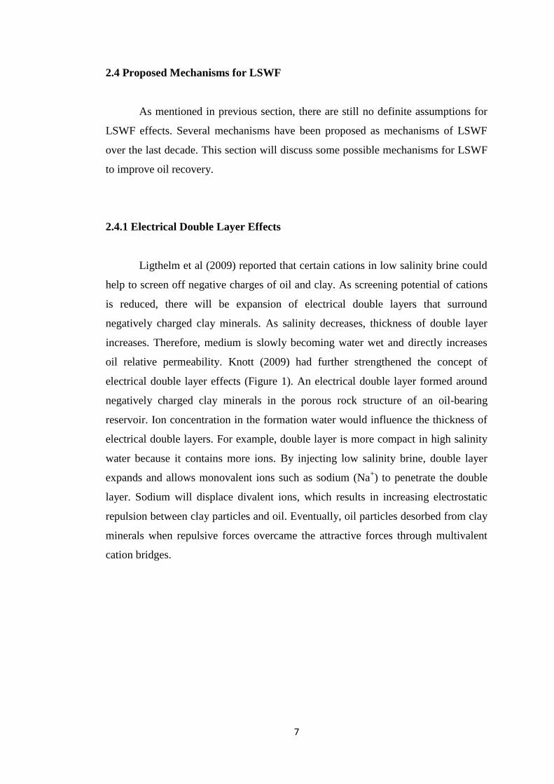
oil relative permeability. Knott (2009) had further strengthened the concept of

electrical double layer effects (Figure 1). An electrical double layer formed around

negatively charged clay minerals in the porous rock structure of an oil-bearing

reservoir. Ion concentration in the formation water would influence the thickness of

electrical double layers. For example, double layer is more compact in high salinity

water because it contains more ions. By injecting low salinity brine, double layer

expands and allows monovalent ions such as sodium (Na+) to penetrate the double

layer. Sodium will displace divalent ions, which results in increasing electrostatic

repulsion between clay particles and oil. Eventually, oil particles desorbed from clay

minerals when repulsive forces overcame the attractive forces through multivalent

cation bridges.

8

In the case of high salinity water containing more ions, the double layer is

more compact but when the low salinity water is introduced, the double layer tend to

expands as seen in Figure 1(1&2)., respectively. The adsorbed layer of positive ions

contains divalent calcium (Ca2+) or magnesium (Mg2+) ions, which acts as tethers

between the clay and oil droplets. Injecting reduced salinity water opens up the

diffuse layer, enabling monovalent ions such as sodium (Na+), carried in the

injection water, to penetrate into the double layer, Figure 1(3). At the same time,

monovalent ions displace the divalent ions as results to increase electrostatic

repulsion between clay particles and oil. It is believed that once the repulsive forces

exceed the binding forces via multivalent cation bridge, the tethers between oil and

clay particles is broken and the oil particles may be desorbed from clay surfaces.

Thus, this will change the wetting state because of the reduction of the rock surface

which is coated by oil and allow the oil to be swept out of the reservoir in

Figure.1(4).

Figure 1: How double layer worked (After Knoott et al.,2009)

9

2.4.2 pH Effect

McGuire et al. (2005) proposed a low salinity recovery mechanism based on the

generation of surfactants from the residual oil at elevated pH levels in accordance

with the observations on the changes in reservoir fluids, fluid/rock interactions and

changes in wettability. A LSWF experiment was conducted from a North Slope

Alaskan field. There was an increased pH from 8 to 10 when low salinity brine was

injected and oil recovery increased from 56% to 73%. Lager et al. (2006) proposed

two possible reactions increasing the pH during low salinity waterflooding

experiments:

Carbonate dissolution resulting in an excess of OH-

(2.1)

(2.2)

Cation exchange between clay minerals and the invading water.

However, cation exchange is faster than carbonate dissolution and the mineral

surface will exchange H+ present in the liquid phase with cations previously

adsorbed, resulting in a pH increase. Austad et al. (2010) gave a clearer view on

relationship of pH and salinity. Due to dissolved acidic gases like CO2, the pH of

formation water of reservoir is around 5. Within this pH, divalent cations from

formation water such as Ca2+

will tend to absorb cation exchange material, which are

the clay minerals. During LSWF ion concentration of injected brine is significantly

lower than initial formation brine. Equilibrium association with the brine-rock is

interaction is disrupted, causing desorption of of Ca2+

from clay. To replace the loss

of Ca2+

ion, H+ ion from water close to the clay surface adsorb onto the clay. There

will be a local increase in pH close to the brine-clay due to the substitution of Ca2+

ion by H+ ion.

10

2.4.3 Fines Migration

Tang and Morrow (1996) have observed production of kaolinite fines along

with the increase in production through LSWF. During LSWF, clay fines are only

partially in contact. Mobilisation of these fines resulted in exposure of underlying

surfaces, which increase water wetness of system. The theory of fines migration is

best illustrated in figure 2. Released of clay minerals could block pore throats and

channelled flowing water into non-swept pores to increase its microscopic efficiency

(RezaeiDoust, 2009b). Moreover, Berea sandstone used by Morrow et al. (1998) for

many of their experiments had predominantly kaolinite clay and quartz. Morrow et al.

(1998) have found out that there are effects on oil recovery when varying the ionic

composition of both the injected and connate brine. However, there were no sign of

fines migration when BP had done various LSWF experiments showing increased in

oil recovery (Lager et al. 2006). So fines migration may be an effect of LSWF

instead of direct cause of increased oil recovery. In brief, fines migration is still vital

in the process of LSWF that increases oil recovery.

11

Figure 2 shows the conditions of residual oil before and after injection of

dilute brine. Initially oil is retained at clay surface due to oil–wet nature of clay

particles. But during LSWF, clay particles are released from the rock surface (solid).

Indirect mobilisation of oil occurs due to mobilisation of the clay particles.

Consequently, residual oil saturation decreases and it leads to flow through less

permeable zones enhancing the sweep efficiency.

Figure 2: Detachment of clay particles and mobilization of oil (Tang, 1998)

12

2.4.4 Multicomponent Ion Exchange (MIE)

Lager et al. (2006) proposed a mechanism based on Multicomponent Ionic

Exchange (MIE) between the invading brine and mineral surface. Positively charged

multivalent ion assists polar oil components to connect to a negatively charged clay

surface. On the other hand, positively charged multivalent ion will release oil

component if it exchanged with a monovalent ion. From the list of mechanisms

published by Sposito (1989) for organic matter absorption onto clay material, Lager

(2006) had identified four out of eight mechanisms that are affected by possible

cation exchange capacity in LSWF. The 4 mechanisms were cation exchange, water

bridging, cation bridging and ligand bridging/bonding. Figure below shows

attraction between clay surface and crude oil by divalent cations. MIE as one of

LSWF mechanisms was proven through coreflooding experiment of the North Slope.

Based on the analysis, salinity of injected brine was lower than the salinity of

connate water. Decreased of concentration of Ca2+ and Mg2+ were reported,

indicating Ca2+ and Mg2+ absorbed by rock matrix.

13

Figure 3 shows the four main mechanisms (cation exchange, cation bridging,

ligand bridging, water bridging) of organic matter adsorption onto clay mineral that

are greatly affected by cation exchange between clay surface and injected water.

Different mechanism has different type of organic functional group. For cation

exchange, organic functional groups involved are amino, ring NH, heterocyclic N

(aromatic ring). Carboxylate, amines, carbonyl and alcoholic OH form the organic

functional group of cation bridging. Conversely, Ligand exchange only consists of

carboxylate while organic functional group for water bridging is the combination

amino, carboxylate, carbonyl and alcoholic OH.

Figure 3: Attraction between clay surface and crude oil by divalent cations ( Lager et al. 2008)

14

2.5 Low Salinity Water Flooding Model

Jerauld at al. (2008) developed a low salinity model which was based on

established modelling approaches for chemical EOR. Modelling of LSWF was

derived from conventional water flood modelling. The salt is modelled as an

additional single lumped component in the aqueous phase which can be injected and

tracked. Salinity will have a significant effect on viscosity and density of aqueous

phase. In addition, function of salinity is dependent on relative permeability and

capillary pressure as well as residual oil saturation. High and low salinity relative

permeability curves are inputs, where shapes are interpolated in between. However,

dependence on relative permeability and capillary pressure are not observed at high

and low salinities. Part of connate water is made inaccessible to suit the conditions of

LSWF effects. In order to model oil bank development, hysteresis between

imbibitions and secondary drainage water relative permeability is included.

On the other hand, Wu et al. (2009) presented a mathematical model for

modelling low-salinity waterflooding in porous or fractured reservoirs. It can be

applied on 1-D, 2-D and 3-D low salinity water flooding simulation. In this

conceptual model, salt is treated as additional “component” to the aqueous phase in

a gas, oil and water three-phase flow system and is transported only within the

aqueous phase by advection and diffusion. Besides, salt is subject to adsorption onto

rock solids. Moreover, interaction between mobile and immobile water zones and

flow in fractured rock are handled using a general multiple-continuum modelling

approach. Same as the model proposed by Jerauld et al. (2008), changes of salinity

will affect its relative permeability, capillary pressure and residual oil saturation.

Omekeh et al. (2012) proposed two phase flow oil and water phases to model

ion-exchange and solubility in LSWF. The model demonstrated impact on water-oil

flow function due to dissolution or precipitation of various carbonate minerals and

multiple ion-exchange (MIE). Relative permeabilities depends on desorption of

divalent ions with the aid of a weighing function. Results from the model proved that

composition of brine is influenced by calcite dissolution and ion exchange.

15

2.6 Summary

All the proposed LSWF mechanisms are related to wettability alteration,

generally towards water-wet conditions. Chemical reactions cause reduction of

residual oil which directly improves oil recovery. Thus, relative permeability and

saturation will be the main parameters in simulation work. Based on literature review

conducted, these parameters are also emphasised in the modelling approach for low

salinity flooding model. Wettability affects both end-point saturations and the shape

of the capillary pressure curve Pc. For instance, it has been shown that intermediate

wettability leads to minimum value for Sor, thus at large scale inducing a higher

recovery. Wettability also changes the shape of the Pc curve. controlled mainly by

the pore size distribution and is not function of wettability, yet the "level" of Pc

depends strongly on wettability: Pc>0 for water-wet systems and Pc<0 for oil-wet

systems. Thus we can define a wettability index WI as the logarithm of the ratio

A2/A1 of the area under the positive to the negative parts of the Pc curve.

16

CHAPTER 3

METHODOLOGY

3.1 Research Methodology

This section consists of project analysis which involves data and information

gathering, as well as reservoir simulation work. Intensive studies are conducted to

gain a better understanding on the subject such as proposed mechanisms for LWSF

effects. Main source of this research is technical papers from ONE PETRO website

under Society of Petroleum Engineers (SPE). Besides, the author also does plenty of

readings on LSWF models. Among the studied LSWF models, one of them will be

selected to perform reservoir simulation work.

Main results from the reservoir simulation focus on changes of recovery

factor which is attributed to changes of salinity in LSWF. Apart from having

research on LSWF technique, studies are also carried out on software which the

author is going to use to simulate reservoir models (Eclipse). In the early stage, the

author will explore and read the manuals for Eclipse 100 software. The author then

starts to familiarize the Eclipse 100 software and the interface. After that the author

is going to start working on the simulation. Simulation work will begin at middle

stage of FYP I to the whole time frame for FYP II. Results and data obtained from

the simulation will be analysed and discussed. Economic analysis will be done to

select the best simulation model. Finally, the author will compile research findings,

literature review and modelling works into project’s final report.

17

3.2 Project Activities

Report Writing

Compilation of all research findings, literature reviews, modelling works and outcomes into a final report

Discussion of Analysis

Discuss the findings from the results obtained and make a conclusion out of the study, determine if the objective has been met

Analysis of Results

Correlate the data obtained from Field Data/Data from Journal papers through simulation studies

Reservoir Simulation Work

Simulate reservoirs using Eclipse 100 based on LSWF case

ECLIPSE 100 Software Setup

Select an appropriate programming software and learn to develop programming code

Preliminary Research

Understanding fundamental theories and concepts, perform literature review, software identification

Title Selection

Selection of the most appropriate final year project title

18

3.3 Gantt Chart and Key Milestones

Table 1: Gantt Chart for First Semester Project Implementation

Key Milestones

Project Activities

FINAL YEAR 1st SEMESTER

(JAN 2013)

No. Detail/ Week 1 2 3 4 5 6 7 8 9 10 11 12 13 14

1 Project title

selection

2. Preliminary

research work

3. Extended proposal

submission

4. Study on

fundamental

concepts related to

the project &

familiarize the

usage of ECLIPSE

100

5. Topic Defence

6. Reservoir

simulation models

using ECLIPSE 100

and economic

analysis

7. Preparation of

interim report

8. Submission of

interim report

Mid

-sem

este

r b

reak

19

Table 2: Gantt Chart for Second Semester Project Implementation

Key Milestones

Project Activities

FINAL YEAR 2nd

SEMESTER

(MAY 2013)

No. Detail/ Week 1 2 3 4 5 6 7 8 9 10 11 12 13 14 15

1 Reservoir

simulation models

using ECLIPSE 100

and economic

analysis

2. Results

Comparison

3. Submission of

Progress Report

4. Economic Analysis

and Selection of

Base Case

5. Preparation of

Final Report

6. Pre-SEDEX

7. Submission of Draft

Report

8. Submission of

Dissertation (soft

bound)

9. Submission of

Technical Paper

10. Oral Presentation

11. Submission of

Project Dissertation

(Hard Bound)

Mid

-sem

este

r b

reak

20

3.4 Low Salinity Water Flooding (LSWF): Options in ECLIPSE 100

Eclipse 100 has a brine tracking function, which has a low salinity option.

This option can be activated by keyword LOWSALT in the RUNSPEC section. The

low salinity option is based on the model described by Jerauld et al. (2008). This

model relates the total salinity of the water to relative permeability curves. They

defined a curve for low salinity water and one for high salinity water. For values

between the curves they interpolate. The interpolation is conducted by a set of

equations as shown below

(3.1)

(3.2)

(3.3)

F1 and F2 represent functions of the salt concentration. krw is the water relative

permeability while oil relative permeability is refered as kro. Pcow is oil-water

capillary pressure. Lastly, subscripts H stands for high salinity curves whereas L

stands for low salinity curves. For end point of saturations, it is calculated by

following sets of equations:

(3.4)

(3.5)

(3.6)

(3.7)

F1 is a function of the salt concentration, and corresponds to the third column of the

LSALTFNC keyword, krw is the water relative permeability, kro is the oil relative

permeability and Pcow is oil-water capillary pressure.

In addition, this model adds an extra separate salt phase to the existing phase,

and a mass conservation equation for the new phase is solved for each grid block in

the reservoir. Brine is assumed to exist only in water phase (Schlumberger, 2011).

21

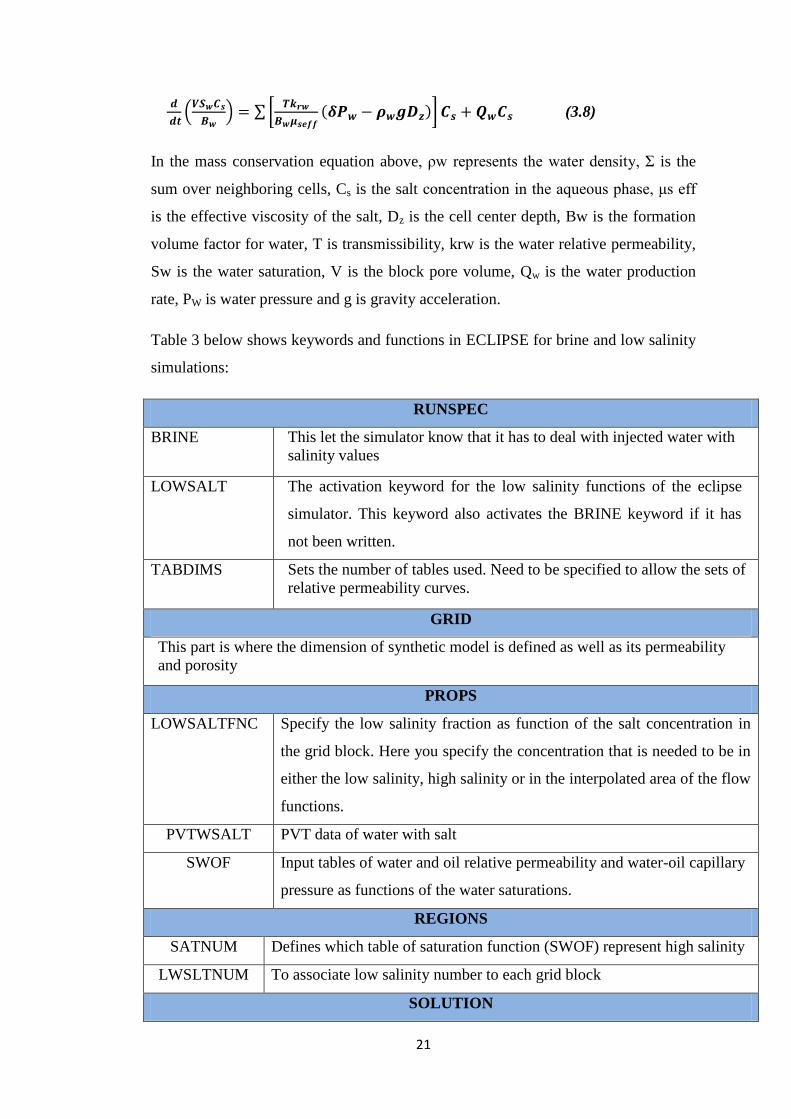
(3.8)

In the mass conservation equation above, ρw represents the water density, Σ is the

sum over neighboring cells, Cs is the salt concentration in the aqueous phase, μs eff

is the effective viscosity of the salt, Dz is the cell center depth, Bw is the formation

volume factor for water, T is transmissibility, krw is the water relative permeability,

Sw is the water saturation, V is the block pore volume, Qw is the water production

rate, PW is water pressure and g is gravity acceleration.

Table 3 below shows keywords and functions in ECLIPSE for brine and low salinity

simulations:

RUNSPEC

BRINE This let the simulator know that it has to deal with injected water with

salinity values

LOWSALT The activation keyword for the low salinity functions of the eclipse

simulator. This keyword also activates the BRINE keyword if it has

not been written.

TABDIMS Sets the number of tables used. Need to be specified to allow the sets of

relative permeability curves.

GRID

This part is where the dimension of synthetic model is defined as well as its permeability

and porosity

PROPS

LOWSALTFNC Specify the low salinity fraction as function of the salt concentration in

the grid block. Here you specify the concentration that is needed to be in

either the low salinity, high salinity or in the interpolated area of the flow

functions.

PVTWSALT PVT data of water with salt

SWOF Input tables of water and oil relative permeability and water-oil capillary

pressure as functions of the water saturations.

REGIONS

SATNUM Defines which table of saturation function (SWOF) represent high salinity

LWSLTNUM To associate low salinity number to each grid block

SOLUTION

22

SALTVD Salt concentration versus depth table

SUMMARY

Don’t have any essential keywords to the simulation here. There are some keywords that

will show you the salt values in the simulation, but they are not needed to run the

simulation. They are however interesting if you want to see how the salinity changes.

SCHEDULE

WSALT Salt concentration for injection well

Table 3: Essential keywords and functions in Eclipse 100 for LWSF simulation

3.5 Synthetic Model and Properties

In this research, synthetic model is of dimension 150 meters, 150 meters and

6 meters in I, J and K directions respectively (Figure 5). Reservoir phase is a two

phase model, oil and water for simplifications. The model is simulated in flood test

by Eclipse 100 (2009.1) with a dimension of 50, 50 and 3 grids blocks. There are 2

wells: Injector and producer which are placed in grid number 1,1,1-3 and 50,50,1-3

respectively. Both wells are controlled by reservoir volume rate (RESV) at 100

m3/day. The model is heterogeneous for the different layers. The Norne reservoir and

fluid properties are used in the simulation(Table 4). The property details are taken

from Emegwalu C.C. (2009), which were used in his enhanced oil recovery flooding

study. Synthetic relative permeability of this model (Omekeh et al., 2012) can be

found in Appendix A. As mentioned in the low salinity option, there can be 2 inputs

for relative permeability and saturation profiles when the low salinity function is

activated in ECLIPSE 100. The first input is to be applied during conventional water

flooding where in this case it is referred as high salinity flooding. Another input will

be used during low salinity water flooding. Keyword SATNUM in the REGIONS

section determines which table of saturation function (SWOF) represents the high

salinity saturation. To define low salinity table, the keyword LWSLTNUM must be

inserted in REGIONS section. Please refer to figure 4 to 6 for the simulated model

showing well placements with initial salt concentration, permeability x,y and z

respectively. Permeability in y direction is not shown in the following figures as they

are the same as the permeability in x direction.

23

Figure 4: Synthetic model with well placements and initial salt saturation distribution

Figure 5: Synthetic model showing permeability Z direction

Figure 6: Synthetic model showing permeability in X direction

24

In this study, capillary pressures were neglected due to lack of data. The experiment

simulated assumes only one salt presents in the brine for simplications. The initial

connate water salinity is set to 35 kg/m3

TDS, approximately the same salinity as

seawater. From the literature review, effect of low salinity waterflooding was only

observed after salinity is decreased significantly below 5000ppm (McGuire, 2005).

Thus, effect of low salinity waterflooding was set at below 5 kg/m3 TDS or 5000ppm

in LSALTFNC table. Moreover, LSALTFNC is also able to decide the amount of

high salinity and low salinity saturation and relative permeability profiles that were

used during injection of brines with different salinities. LSALTFNC table is found in

table 5 below.

Salt Concentration

(kg/m3)

Salinity

(ppm)

F1

F2

0 0 1 1*

1 1000 0.8 1*

4 4000 0.2 1*

5 5000 0 1*

35 35000 0 1*

Table 5: LSALTFNC for the synthetic model

FLUID PROPERTIES

Oil Density 860 kg/m3

Water Density 1033 kg/m3

Gas Density 0.853 kg/m3

Water Formation Volume Factor (Bw) 1.038

Water Viscosity 0.318

Compressibility factor 4.67E-5

ROCK PROPERTIES

Permebility in I and J Directions 1172,1143 and 1162 (md)

Permeability in Z Direction 1050, 1800 and 500 (md)

Porosity 0.3

Reservoir Pressure 277 Bar

Compressibility 4.67 E-5

Table 4: North E-Segment Rock and Fluid Properties used for simulation

25

3.5 Studied Cases

The reference case or the base case is the case that uses high salinity (HS)

water flooding technique from the starting to the end of production, totally 10 years

or 3650 days. Since we injected continuous (HS) water flooding or brine 35000ppm

from the first day to the last day of production, the same way with continuous low

salinity (LS) or brine 1000 ppm is done in order to compare the effect of salinity in

general with the base case. Then, the effect of timing for secondary recovery phase is

studied by using HS as the first phase and changing the starting day of continuous

LS injection for the second phase. The best result of timing study is continued using

for varying the salinity of LS in the tertiary recovery phase. The low salt

concentration that could give the reasonable recovery is chosen and is used for all

simulation cases in economic analysis. The last scenario is to change the size of LS

slug in the second phase, while keeping the same HS flooding in the first phase, the

day of starting LS slug and HS flooding for the tertiary phase recovery. The main

purpose of doing this is to find out the best time to start and cease low salinity

injection, in order to maximize profit while minimizing fresh water injection cost.

The most reasonable case will then be chosen after evaluating its economic

feasibility.

26

3.6 Simulation Study Work Flow

Simulation Study Work Flow Key Milestones

Date Gathering Week 10 (FYP I)

Base Case Study Week 13 (FYP I)

Simulation on Different Cases Week 3 (FYP II)

Results Comparison Week 4 (FYP II)

Economic Analysis and Selection of base case Week 7 (FYP II)

Data Gathering

-Modelling approach based

on Jerauld et al., 2008

-Reservoir data extracted

from Emegwalu, 2009

Base Case Study

-High salinity(HS) continuous

flooding (35000ppm) for 10 years

-Low salinity(LS) continuous

flooding (1000ppm) for 10 years

(1000ppm)

Simulation of Different Cases (HS+LS)

-Alternate the flooding days for LS

and HS

-Alternate concentration for LS

(1000-35000ppm) while fixing

flooding days for HS

Results Comparison

-Compare each case by its oil

recovery factor, oil production

rate, cumulative oil production,

salt production rate, etc

Economic Analysis

-Selection of some ideal LSWF

cases for simple economic

analysis

Selection of the Best Case

-The best case will be selected

after being justified by its

findings and economic analysis

Table 6: Key milestones for simulation study work flow

27

3.7 Tools Required

1) ECLIPSE Software (2009.1)

- Developed by Schlumberger for reservoir simulation purposes

- Focuses on black oil model (ECLIPSE 100)

Figure 7: ECLIPSE simulation software launcher 2009.1

2) Hand tools

- Pencil, pen, highlighter, calculator, etc.

3) Microsoft Word 2007

- To prepare report and notes

4) Microsoft Power Point 2007

- To prepare presentation slides

28

CHAPTER 4

RESULTS AND DISCUSSIONS

4.1 Effect of LSWF in Secondary Recovery Phase

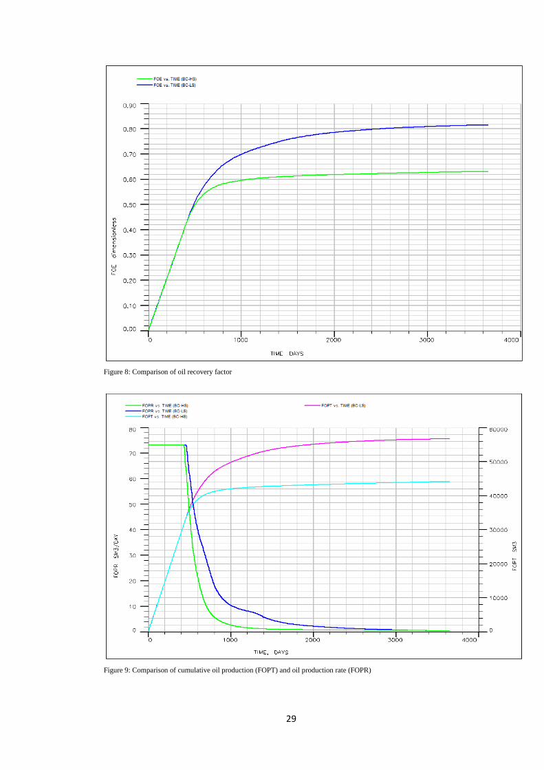
4.1.1 Effect of the Salinity on Recovery Factor

From Figure 8, it can be seen that the recovery factor gets to 81.7% for the

base case with continuous low salinity water flooding while the base case with high

salinity water flooding gives only 63.5% recovery factor. This indicates oil recovery

improves with a decrease in salinity of the injected brines. The 63.5% for the high

salinity base is considered quite high as the simulated model is homogenous for the

same layer, leading to a better sweep efficiency of the reservoir.

4.1.2 Effect of salinity on Oil Production Rate and Cumulative Oil Production

Figure 9 shows the effect of salinity in water flooding on oil production rate

and cumulative oil production. From the graph, it is seen that a certain period of time

is needed before the effect of the low salinity injection takes place. Cumulative Oil

Production for LS base case is 56763 sm3

while 44612 sm3

is recorded for HS base

case. Thus, the oil production rate of LS base case has been higher than HS base case.

Cumulative oil production is increasing steadily for both cases until 2000 production

days where production starts to be stagnant. Both cases maintain their oil production

rates constant until they fall drastically. This means water breakthroughs are reached

at 460 days for HS base case and at 430 days for LS base case. This shows that

around 430 days are needed for low salinity effect to become visible. The shorter the

time for low salinity effect to appear, the better it becomes for the economics.

29

Figure 8: Comparison of oil recovery factor

Figure 9: Comparison of cumulative oil production (FOPT) and oil production rate (FOPR)

30

4.1.3 Comparison of Salt Production Rate and Salt Production Concentration

Salt production rate (figure 10) and salt production concentration (figure 11)

clearly follow the injected concentration. Salt production rate and salt production

concentration remains constant throughout the production life for HS base case. On

the contrary, salt production concentration for LS base case is decreasing gradually

until 2000 production days where it stays at about 1 kg/m3 throughout the rest of

production days. However as mentioned in section 4.2, low salinity effects only

occur after some times from initial injection, around 430 days. This time is also

suspected to be the time where water breakthrough. After that, salt production rate

still increases slowly and then declines sharply after 560 production days.

4.1.4 Summary of LSWF Simulation Results in Secondary Recovery Phase

The base cases work well, and most of the results are as expected. Due to the

initialization of the model, most of the results are also easy to predict. The effect of

the low salinity water flooding is very high for the simulated cases. This model is

homogenous for the same layer; therefore this made the predictions even easier. The

only heterogeneity in this model was seen in the layer depth. No transmissibility or

permeability barriers were included such as faults or impermeable zones. This

clearly optimizes the effect of low salinity water flooding, because the injected fluids

can flow easily through the reservoir and displace the oil.

31

Figure 10: Comparison of salt production concentration

Figure 11: Comparison of salt production rate

32

4.2 Effect of LSWF in Tertiary Recovery Phase

4.2.1 Effect of Timing of LS injection on Recovery Factor and Oil Production

Rate

This part is focused on interval of primary HS injection and time to start

secondary injection by LS water. Since we have chosen 1000ppm as LS base case

while 35000ppm as HS base case, they would continue to be used in examining the

effect of LSWF in secondary recovery phase. The ultimate recoveries will be the

study parameter in this phase. Due to time constraint, only 3 different intervals are

chosen to investigate the effect of LSWF in secondary phase. The day to start

secondary phase are selected at 300 days (300HS-3350LS), 450 days (450-HS-

3200LS) and 600 days (600HS-3050LS) after starting production with HS flooding –

with 3350 days, 3200 days and 3050 days of continuous LSWF , respectively.

From figure 12, the graph shows that earlier the LS injection, the higher oil

recovery as a result from the longer LS continuing flooding period. Oil recovery

results at the end of production life are 80.81%, 80.63% and 80.46% in order of the

first LS injection day after HS flooding at 300 days, 450 days and 600 days. The

incremental cumulative oil recoveries from HS base case are 17.31%, 17.13% and

16.96%. However, they are less than the total cumulative oil from LS base by 2.19%,

2.37% and 2.54% respectively. The 3 cases are not seen clearly different from each

other at the beginning until about 715 production days. However, 3 cases have

almost the same oil recovery at the end of production after LSWF take place.

Through figure 13, it can be noticed that LS injection at 300 days gives the earliest

effect followed by LS injection at 450 days and at 600 days. Hence, oil production

rate does not drop as much as the other cases. Oil production rate keeps constant for

a while and starts to fall again gradually at 945 days until becoming constant from

2595 production days. Generally, all the 3 cases have the same trend of oil

production rate that drop steadily before low salinity brine is injected into the field.

After LSWF occurs, oil production rate increases for about 275 days before descend

again there upon. At the end of production life, oil production rate and from three

cases become almost the same value.

33

Figure 12 Effect of Timing of LS injection in Secondary Recovery Phase

Figure 13 Effect of Timing of LS injection on Field Oil Production Rate (FOPR)

34

4.2.2 Effect of Salinity Concentration in Tertiary Recovery Phase

This section is to investigate the effect of varying salinity in LSWF on its

tertiary recovery phase. Based on the 3 cases studied in section 4.2.1, the case where

LS injection at 300 days is chosen as the base case to investigate the effect of salinity

in tertiary imbibitions. The tertiary recovery was done by flooding of brines with

salinities of 35000, 5000, 4000, 3000, 2000, and 1000 ppm. The results of recovery

factor from the injection of different brine salinities are presented in figure 14 and

the ultimate recoveries are tabulated in table 6.

Injected Brine Salinity (Ppm) Recovery Factor (%)

1000 80.46

2000 76.13

3000 71.45

4000 66.76

5000 63.50

35000 63.50

Table 8: Results of recovery factor from different injected brine salinities

As predicted from the model, there is no incremental oil recovery for

injection of brines with salinities above 5000ppm. This is because the low salinity

effect is set to start at salinities below 5000ppm in LSALTFNC table. Regarding to

the oil recovery, an increase in recovery is seen in conjunction with a decrease in

salinity. This phenomenon is the same as the literature review discussed in previous

section. It is noted that both the rate of recovery and ultimate recovery increased

with a decrease in salinity of the injected brines. From figure 15, we can see a range

of increasing in oil production rate. Oil production rate showing that oil can be

produced at a higher rate is salinity is lower. Moreover, there will be a longer LSWF

effect if the salinity is lower. Both figures show a big gap between salinity 1000 ppm

and 5000 ppm that are expected to be the lower and the upper thresholds (Jerauld et

al, 2008).

35

Figure 14 Effect of salinity concentration on recovery factor in tertiary recovery phase

Figure 15 Effect of salinity concentration on oil production rate in tertiary recovery phase

36

Figures below represent the residual oil sweeping efficiency for base case with

continuous low salinity water flooding from 1st

year until 10th

year production in one

of the x and z plane directions:

Oil Saturation

Figure 16 First year oil saturation distribution

Figure 17 Second year oil saturation distribution

Figure 18 Third year oil saturation distribution

Figure 19 Fourth year oil saturation distribution

37

Oil Saturation

Figure 20 Fifth year oil saturation distribution

Figure 21 Sixth year oil saturation distribution

Figure 22 Seventh year oil saturation distribution

Figure 23 Eighth year oil saturation distribution

38

Oil Saturation

Figure 24 Ninth year oil saturation distribution

Figure 25 Tenth year oil saturation distribution

From figure 16 to figure 25, it is shown that low salinity water flooding affects the

oil saturation of the field by reducing the oil saturation from 85% to around 15%.

After looking at the displacement of residual oil due to low salinity effect, it shows

that different layers of reservoir will have different time for their oil displacement.

This is mainly due to the permeability difference across the layers of reservoir. By

looking at the graphs, wettability of the reservoir is changing from oil-wet to water-

wet. Hence, alteration of wettability plays a vital role in determing the efficiency of

LSWF. In addition, effects of salinity concentration on oil distribution are also

portrayed through the FLOVIZ models in the following pages.

39

Figures below represent oil saturation distribution at the end of 10 years production

for different salinity concentration:

Figure 26 Injection of brine with salinity of 1000ppm

Oil Saturation

Figure 27 Injection of brine with salinity of 2000ppm

40

Figure 28 Injection of brine with salinity of 3000ppm

Oil Saturation

Figure 29 Injection of brine with salinity of 4000ppm

41

Figure 30 Injection of brine with salinity of 5000ppm

Oil Saturation

Figure 31 Injection of brine with salinity of 35000ppm

42

4.2.3 Summary of LSWF Simulation Results in Tertiary Recovery Phase

An increase in oil recovery is seen in conjunction with an earlier injection

time. This is as expected because an early injection time means injection of more

low salinity brines and this should increase the effectiveness of the LSWF. The

difference in ultimate recovery is however not very large compared to the rate of

recovery. Oil saturation decreases when salinity of injected brine reduces.

Nevertheless, alteration of wettability is still a main factor behind LSWF effects.

Through the findings and discussions in section 4.2.1 and 4.2.2, it has shown that LS

injection needs transition time to achieve its effect. Furthermore, the effects will only

occur for some period on oil production rate where it becomes constant afterwards.

In summary, using 35000ppm salinity in HS flooding as primary phase for 300 days

and continuing with 1,000ppm salinity in LS flooding as secondary flooding (HS-LS)

is the most reasonable case for the tertiary recovery phase study.

43

4.3 Sensitivity Study of LSWF Economics

4.3.1 Economic Evaluation

In reality, LSWF will not be applied continuously throughout the field’s

production lifetime. This is due to the economic feasibility in terms of equipment

cost and operation cost. Moreover, flooding with low salinity for whole production

life may cause economic issues when incremental oil recovery is not high enough.

Consequently, the profits generated from increased oil recovery will not cover its

cost. In this section, the most reasonable case discussed in section 4.2 will be used

for sensitivity study of LSWF economics.

Basically, the success of an EOR process is determined by the amount of

incremental oil recovered. For a low salinity water flooding project, the EOR oil will

be incremental oil recovery over conventional water flooding which is high salinity

flooding in our base case. To determine the best case to perform our low salinity

water flooding project, the Net Present Value (NPV) criterion is selected. The NPV

calculation is based on incremental oil production from low salinity water flooding

compared to conventional water flooding (High salinity).

NPV is a central tool in discounted cash flow (DCF) analysis, and is a

standard method for using the time value of money to appraise long-term projects.

The NPV must be positive for a project to be accepted. It is defined by the formula

(4-1)

where r is the discount rate, t is the time, Ct cash flow in year t, and n is time period

of the project/investment.

According to the economic sensitivity study done by Chuck Kossak(2012) in

his LSWF study, the main interest should be focused in the incremental oil recovery

from low salinity water flooding case over the incremental oil recovery from

continuous high salinity water flooding. Furthermore, he has come out with a simple

cost analysis formula. The following formula will be inserted into Eclipse data file in

order to generate a profit versus time graphs for different cases (Figure 32). Besides,

some assumptions need to be considered before performing the economic analysis.

44

Assumptions for Economic Evaluation:

a) The simulated model is assumed to be producing at its residual oil saturation.

b) Provided properties of low salinity brine are compatible with the synthetic

model’s reservoir and fluid properties.

c) 3 different cases will be selected to examine the economic sensitivity of LSWF:

Scenario 1: Continuous Low Salinity Flooding throughout production

lifetime (Low salinity base case in section 4.1)

Scenario 2: Initial high salinity flooding with constant high salinity

concentration of 35000ppm for 300 days before flooding with constant low

salinity concentration of 1000ppm continuously for the rest of production

lifetime (Best case chosen in section 4.2)

Scenario 3: Best time to stop low salinity injection in scenario 2 in order to

maximise profit or Net Present Value(NPV)

d) The assumed discount rate, price of oil and price of fresh water through

desalination are given in table. Cost of high salinity water is zero as it is easily

obtained from sea water.

e) For simplification, only cost of fresh water through desalination is considered as

major expense of the LSWF project. No operational and additional facilities

costs are considered. Moreover, fluctuation of oil price, discount factor, interest

rates and inflation are not included in this economic analysis.

f) All the NPV analysis is done using ECLIPSE software. The plotted graphs will

be used to determine the breakeven year, net profit and best case to do LSWF.

Oil Price (Income) $500/sm3

Fresh Water Through Desalination $15/sm3

45

UDQ

ASSIGN FUOIL 500 / oil price ($/Sm3)

ASSIGN FUFW 15 / fresh water cost ($/Sm3)

ASSIGN FUSWOE 44612 / oil produced by high salt water (Sm3)

DEFINE FUPROFIT (FOPT-FUSWOE)*FUOIL-(WWIT

IFRESH)*FUFW / profit ($)

UNITS FUPROFIT $ /

UPDATE FUPROFIT ON /

Figure 32: ECLIPSE functions for sensitivity study of LSWF economic simulations

Firstly, keyword FUOIL represents oil price which is set at $500 per sm3.

FUFW symbolises fresh water injection cost at $15 per sm3. FUSWOE is the amount

of oil produced by high salinity or conventional water flooding. FUSWOE is

considered as the expense of carrying out low salinity water flooding project. In

order to calculate the NPV, subtract FUSWOE from the amount of oil recovered

through low salinity flooding (FOPT) before multiplying by the oil price (FUOIL).

After that, the profit (FUPROFIT) is computed by deducting the amount of fresh

water injected into the well (WWIT IFRESH) multiply by the cost of fresh water

(FUFW).

For example, FOPT is assumed to recover 54612sm3 of oil while the amount

of injected water is 35000sm3. Through the function of FUPROFIT, calculated NPV

will be $475,000.

(FOPT-FUSWOE)*FUOIL-(WWIT IFRESH)*FUFW

= (54612-44612)*$100 – (35000)*$15

= $ 475,000

In the following sections, NPV graphs will be generated for 3 different cases.

These graphs will be useful to find out the breakeven year where the LSWF project

starts to gain profit. Moreover, the total net profit will be vital to select the base case

for this LWSF study.

46

4.3.2 Economic Simulation Results and Analysis

4.3.2.1 Scenario 1: Continuous Low Salinity Water Flooding

In this case, the simulated is flooded with low salinity brine throughout its

production lifetime for 10 years. Total amount of NPV and injected fresh water is as

shown in figure 33. Although first year of NPV recorded -22.6 million USD, the

total incremental of NPV is positive and the figure is +9.10 million USD. Payback

period or breakeven takes about 2.5 years.

4.3.2.2 Scenario 2: Initial High Salinity Flooding for 300 days followed by

Continuous Low Salinity Water Flooding

This scenario is selected from the best case discussed in section 4.2. Total

amount of NPV and injected fresh water is as shown in figure 33. Although first year

of NPV recorded -22.6 million USD, the total incremental of NPV is positive and the

figure is +7.88 million USD. Payback period or breakeven takes about 3.4 years.

Although NPV of scenario 1 is higher than scenario 2, NPV of scenario 1

after 6th

year onwards is slightly higher than NPV of scenario 2. Moreover, amount

of injected fresh water for scenario is significantly higher than that in scenario 2 by

31000 sm3. It will be a waste to inject such a big portion of fresh water when NPV is

decreasing from year to year. This indicates that both scenarios will be uneconomical

in the long run to flood the field continuously with low salinity brine. Therefore,

another scenario needs to be simulated to maximise the NPV while reducing the cost

of injected fresh water by reducing the amount of injected fresh water.

47

Figure 33: Total amount of NPV and fresh water injection for scenario 1 and 2

48

4.3.2.3 Scenario 3: Initial High Salinity Flooding for 300 days followed by

Continuous Low Salinity Water Flooding for 2000 days before Converting it to

High Salinity Flooding for the Rest of Production Lifetime

This scenario is selected from the best time to stop low salinity injection in

scenario 2 in order to maximise profit or NPV. Based on figure 34, the optimum

NPV is around 5.5 years for scenario 1 and 2. Hence, to optimise NPV, low salinity

brine should stop injecting into the well around 2000 days which are close to 5.5

years. After 5.5 years, low salinity flooding should cease but the field should be

injected with high salinity brine to recover residual oil. Figure 34 compares the

amount of NPV and the injected fresh water among the 3 scenarios. The incremental

of Scenario 3 NPV is positive and the figure is +11.01 million USD, which is clearly

higher than the NPV of scenario 1 and 2. Even until the end of production, scenario 3

still remains at a steady yet high NPV. In addition, amount of injected fresh water in

scenario 3 is comparatively lower than the other 2 scenarios by almost 50%.

Breakeven of the year is also fairly early, which is around 3.4 years.

4.3.3 Summary of Economic Simulation Results and Analysis

To optimise LSWF project, economic feasibility must be considered carefully

apart from the total oil recovery. The ideal scenario will be having a high NPV while

having a short payback period. Furthermore, amount of injected fresh water should

be reduced as much as possible without compromising much on the oil recovery.

Scenario 3 is the best case to carry out the LSWF project. This is because the NPV is

the highest among the 3 scenarios. Besides, it only uses almost half of the amount of

injected fresh water compared to other scenarios. Figure 35 shows that

cumulative oil production for the 3 scenarios. Scenario 1 recovers more oil in early

years but at the end of production, total recovered oil is almost the same for all

scenarios. Therefore, it would be a bad decision to select scenario 1 or 2 as there is

not much increase in oil recovery despite injecting more than 50% amount of fresh

water compared to scenario 3.

49

Figure 34: Total amount of NPV and fresh water injection for scenario 1,2 and 3

Figure 35: Cumulative oil production for 3 scenarios

50

CHAPTER 5

CONCLUSIONS AND RECOMMENDATIONS

5.1 Conclusions

This project is able to be completed within given time frame to meet the

relevant objectives. Literature review conducted has enabled the author to have

better understanding on low salinity water flooding concepts as well as modelling

approaches for low salinity model. In addition, there are also detailed research

methodology and simulation work flow to execute this project. This project is able to

achieve all the key milestones, which are vital in preparing an efficient yet effective

report.

The author has familiarised with ECLIPSE 100 where he is able to simulate

LSWF model. The BRINE option in ECLIPSE 100 is dependent on relative

permeability, especially residual oil saturation. This is mainly due to ECLIPSE 100’s

low salinity modelling approach is based on Jerauld et al. (2008). Therefore,

ECLIPSE 100 emphasises on wettability alteration, as mentioned in literature review.

Base case for LSWF model has been identified and it is useful to simulate different

cases in order to examine the effects of salinity on oil recovery and sweep efficiency.

Through initial simulation work until tertiary recovery phase, the author has

found out that there is an improvement in oil recovery with a decrease in salinity.

Although the simulated model is just a synthetic model, it has clearly shown the

potential of LSWF as an EOR mechanism. Last but not least, economic analysis has

shown that scenario 3 will be the best case to perform LSWF while not

compromising on its cumulative oil production.

51

5.2 Recommendations for Future Work

This project only focuses on simulation of a synthetic model. Oil recovery

increases drastically due to homogeneities of the model. However, in real field

situation, most of the reservoirs are heterogeneous with complex permeability

barriers such as fault. Therefore in the future research, a full field reservoir data

should be applied to investigate the potential of LSWF. The project can also be

expanded by adding more salts and ions into the simulation.

On the other hand, Schlumberger (owner of ECLIPSE) should create a new

low salinity function based on the modelling work of Omekeh et al. (2012). The

current low salinity function is only based on modelling work of Jerauld et al. (2008).

If the interpolation of salinity curves is based on ion exchange of certain ion,

multicomponent ion exchange mechanisms can be studied more thoroughly. To

increase the accuracy of the results, findings from ECLIPSE100 should be compared

with findings obtained from other reservoir simulators. Last but not least, this project

can be used as a foundation to simulate other EOR flooding project such as alkali,

surfactant, polymer as well as ASP flooding.

52

REFERENCES

(1) Abeysinghe, K. P., I. Fjelde, et al. (2012). Dependency of Remaining Oil

Saturation on Wettability and Capillary Number. SPE Saudi Arabia Section

Technical Symposium and Exhibition. Al-Khobar, Saudi Arabia, Society of

Petroleum Engineers.

(2) Agbalaka, C., A. Dandekar, et al. (2009). "Coreflooding Studies to Evaluate the

Impact of Salinity and Wettability on Oil Recovery Efficiency." Transport in Porous

Media 76(1): 77-94.

(3) Austad, T., Rezaei Doust, A. and Puntervold, T., 2010, Chemical Mechanism of

Low Salinity Water Flooding in Sandstone Reservoirs, Paper SPE 129767 presented

at the 2010 SPE Improved Oil Recovery Symposium held in Tulsa, Oklahoma, USA,

24-28 April.

(4) C.C. Emegwalu, 2009. Enhanced Oil Recovery: Surfactant Flooding as A

Possibility for the Norne E Segment.

(5) Green, D. W. and G. P. Willhite (1998). Enhanced oil recovery. Richardson, TX,

Society of Petroleum Engineers.

(6) Jerauld, G.R., Lin, C.Y., Kevin J. Webb, and Jim C. Seccombe., 2008, Modeling

Low-Salinity Waterflooding, Paper SPE 102239 presented at Conference and

Exhibition, San Antonio, Texas, 24–27 September

(7) Kossack C., 2012, Eclipse Black Oil Simulator – Advanced Options: Low

Salinity Water Flooding, Denver, Colorado.

53

(8) Lager A., W.K.J., Black C. J. J., Singleton M., Sorbie K. S., 2006. Low Salinity

Oil Recovery An experimental investigation. Paper SCA2006-36 presented at the

International Symposium of the Society of Core Analysts held in Trondheim,

Norway 12-16 September.

(9) Lager A., W.K.J., Collins, I.R., Richmond, D.M., 2008. LoSalTM

Enhanced Oil

Recovery: Evidence of Enhanced Oil Recovery at the Reservoir Scale. Paper SPE

113976 presented at the 2008 SPE/DOE Improved Oil Recovery Symposium held in

Tulsa, Oklahoma, USA, 19-23 April.

(10) Lehne, H.H., 2009, Low Salinity Waterflooding: An Experimental Analysis of a

North Sea reservoir rock, Master Thesis, Norwegian University of Science and

Technology, June 2010.

(11) Ligthelm, D.J. et al., (2009). Novel Waterflooding Strategy By Manipulation Of

Injection Brine Composition, EUROPEC/EAGE Conference and Exhibition. Society

of Petroleum Engineers, Amsterdam, The Netherlands.

(12) Morrow, N. and Buckley, J., 2011, Improved Oil Recovery by Low-Salinity

Waterflooding, Paper SPE 129421.

(13) Omekeh, A., SPE, Friis, H. A., Fjelde, I. & Evje, S. 2012. Modeling of Ion-

Exchange and Solubility in Low Salinity Water Flooding. SPE Improved Oil

Recovery Symposium. Tulsa, Oklahoma, USA: Society of Petroleum Engineers.

(14) McGuire P.L., SPE, Chatham J.R., Paskvan, F.K., SPE, Sommer, D.M., SPE,

Carini, F.H., SPE, BP Exploration (Alaska) Inc., 2005. Low Salinity Oil Recovery:

An Exciting New EOR Opportunity for Alaska’s North Slope. Paper was presented

at 2005 SPE Western Regional Meeting held in Irvine, CA, U.S.A., 30 March-1

April 2005.

54

(15) Reiter, P.K., 1961, A Water-Sensitive Sandstone Flood Using Low Salinity

Water, MSc Thesis, University of Oklahoma, Norman, Oklahoma, USA.

(16) Robertson, E.P, 2007, Low-Salinity Waterflooding to Improve Oil Recovery —

Historical Field Evidence, Paper SPE 109965.

(17) Rezaei Doust, A., Puntervold, T. and Austad, T., 2010, A Discussion of the

Low-Salinity EOR Potential for a North Sea Sandstone Field, Paper 134459

presented at the SPE Annual Technical Conference and Exhibition, Florence, Italy,

19-22 September 2010.

(18) Selboe, K., 2010, Low Salinity Waterflooding in North Sea Reservoir rock: An

Experimental Investigation with Emphasis on Wettability Effects, Master Thesis,

Norwegian University of Science and Technology, June 2010.

(19) Tang, G., and Morrow, N.R, 1997, Salinity, Temperature, Oil Composition and

Oil Recovery by Waterflooding, SPE Reservoir Engineering (November), pp. 269-

276.

(20) Tang, G.Q., and Morrow, N.R., 1996, Effect of Temperature, Salinity and Oil

Composition on Wetting Behavior and Oil Recovery by Waterflooding, Paper SPE

36680.

(21) Zhang, Y., Xie, X., and Morrow, N.R., 2007, Waterflood performance by

injection of brine with different salinity for reservoir cores, Paper SPE 109849

presented at the 2007 SPE Annual Technical Conference and Exhibition, Anaheim,

11–14 November.

(22) Zolotuchin, A. B. and J.-R. Ursin (2000). Introduction to petroleum reservoir

engineering. Kristiansand, Høyskoleforl.

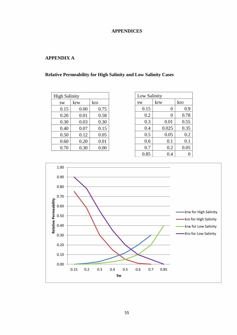
55

APPENDICES

APPENDIX A

Relative Permeability for High Salinity and Low Salinity Cases

High Salinity

sw krw kro

0.15 0.00 0.75

0.20 0.01 0.58

0.30 0.03 0.30

0.40 0.07 0.15

0.50 0.12 0.05

0.60 0.20 0.01

0.70 0.30 0.00

0.00

0.10

0.20

0.30

0.40

0.50

0.60

0.70

0.80

0.90

1.00

0.15 0.2 0.3 0.4 0.5 0.6 0.7 0.85

Re

lati

ve P

erm

eab

ility

Sw

krw for High Salinity

kro for High Salinity

krw for Low Salinity

Kro for Low Salinity

Low Salinity

sw krw kro

0.15 0 0.9

0.2 0 0.78

0.3 0.01 0.55

0.4 0.025 0.35

0.5 0.05 0.2

0.6 0.1 0.1

0.7 0.2 0.05

0.85 0.4 0

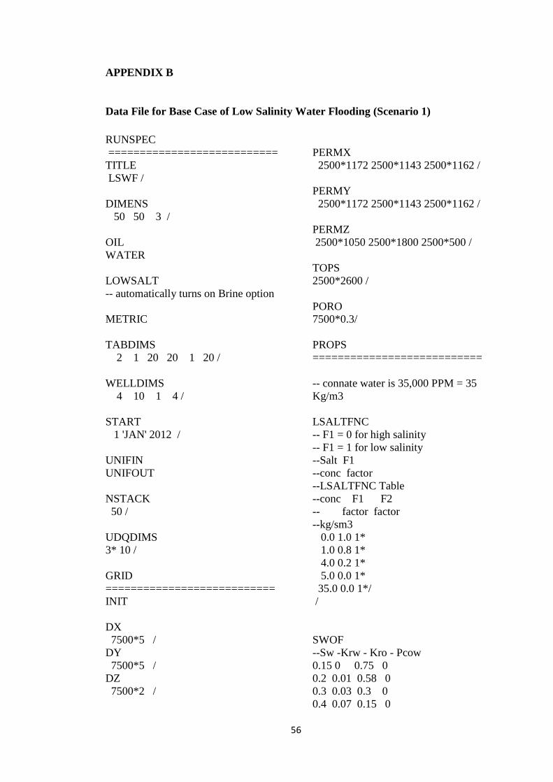
56

APPENDIX B

Data File for Base Case of Low Salinity Water Flooding (Scenario 1)

RUNSPEC

===========================

TITLE

LSWF /

DIMENS

50 50 3 /

OIL

WATER

LOWSALT

-- automatically turns on Brine option

METRIC

TABDIMS

2 1 20 20 1 20 /

WELLDIMS

4 10 1 4 /

START

1 'JAN' 2012 /

UNIFIN

UNIFOUT

NSTACK

50 /

UDQDIMS

3* 10 /

GRID

===========================

INIT

DX

7500*5 /

DY

7500*5 /

DZ

7500*2 /

PERMX

2500*1172 2500*1143 2500*1162 /

PERMY

2500*1172 2500*1143 2500*1162 /

PERMZ

2500*1050 2500*1800 2500*500 /

TOPS

2500*2600 /

PORO

7500*0.3/

PROPS

===========================

-- connate water is 35,000 PPM = 35

Kg/m3

LSALTFNC

-- F1 = 0 for high salinity

-- F1 = 1 for low salinity

--Salt F1

--conc factor

--LSALTFNC Table

--conc F1 F2

-- factor factor

--kg/sm3

0.0 1.0 1*

1.0 0.8 1*

4.0 0.2 1*

5.0 0.0 1*

35.0 0.0 1*/

/

SWOF

--Sw -Krw - Kro - Pcow

0.15 0 0.75 0

0.2 0.01 0.58 0

0.3 0.03 0.3 0

0.4 0.07 0.15 0

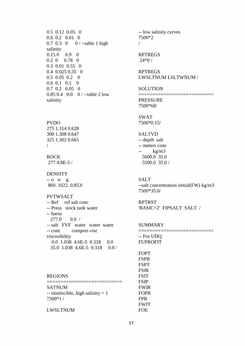
57

0.5 0.12 0.05 0

0.6 0.2 0.01 0

0.7 0.3 0 0 / --table 1 high

salinity

0.15 0 0.9 0

0.2 0 0.78 0

0.3 0.01 0.55 0

0.4 0.025 0.35 0

0.5 0.05 0.2 0

0.6 0.1 0.1 0

0.7 0.2 0.05 0

0.85 0.4 0.0 0 / --table 2 low

salinity

PVDO

275 1.314 0.628

300 1.308 0.647

325 1.302 0.665

/

ROCK

277 4.8E-5 /

DENSITY

-- o w g

860. 1022. 0.853/

PVTWSALT

-- Ref ref salt conc

-- Press stock tank water

-- barsa

277.0 0.0 /

-- salt FVF water water water

-- conc compres visc

viscosibility

0.0 1.038 4.6E-5 0.318 0.0

35.0 1.038 4.6E-5 0.318 0.0 /

REGIONS

===========================

SATNUM

-- immiscible, high salinity = 1

7500*1 /

LWSLTNUM

-- low salinity curves

7500*2

/

RPTREGS

24*0 /

RPTREGS

LWSLTNUM LSLTWNUM /

SOLUTION

===========================

PRESSURE

7500*68/

SWAT

7500*0.15/

SALTVD

-- depth salt

-- meters conc

-- kg/m3

5000.0 35.0

5500.0 35.0 /

SALT

--salt concentration initial(FW) kg/m3

7500*35.0/

RPTRST

'BASIC=2' FIPSALT SALT /

SUMMARY

===========================

-- For UDQ

FUPROFIT

FOPT

FSPR

FSPT

FSIR

FSIT

FSIP

FWIR

FOPR

FPR

FWIT

FOE

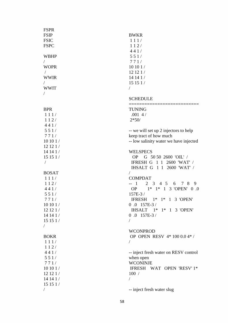
58

FSPR

FSIP

FSIC

FSPC

WBHP

/

WOPR

/

WWIR

/

WWIT

/

BPR

1 1 1 /

1 1 2 /

4 4 1 /

5 5 1 /

7 7 1 /

10 10 1 /

12 12 1 /

14 14 1 /

15 15 1 /

/

BOSAT

1 1 1 /

1 1 2 /

4 4 1 /

5 5 1 /

7 7 1 /

10 10 1 /

12 12 1 /

14 14 1 /

15 15 1 /

/

BOKR

1 1 1 /

1 1 2 /

4 4 1 /

5 5 1 /

7 7 1 /

10 10 1 /

12 12 1 /

14 14 1 /

15 15 1 /

/

BWKR

1 1 1 /

1 1 2 /

4 4 1 /

5 5 1 /

7 7 1 /

10 10 1 /

12 12 1 /

14 14 1 /

15 15 1 /

/

SCHEDULE

===========================

TUNING

.001 4 /

2*50/

-- we will set up 2 injectors to help

keep tract of how much

-- low salinity water we have injected

WELSPECS

OP G 50 50 2600 'OIL' /

IFRESH G 1 1 2600 'WAT' /

IHSALT G 1 1 2600 'WAT' /

/

COMPDAT

-- 1 2 3 4 5 6 7 8 9

OP 1* 1* 1 3 'OPEN' 0 .0

157E-3 /

IFRESH 1* 1* 1 3 'OPEN'

0 .0 157E-3 /

IHSALT 1* 1* 1 3 'OPEN'

0 .0 157E-3 /

/

WCONPROD

OP OPEN RESV 4* 100 0.0 4* /

/

-- inject fresh water on RESV control

when open

WCONINJE

IFRESH WAT OPEN 'RESV' 1*

100 /

/

-- inject fresh water slug

59

WSALT

IFRESH 1.0 /

/

-- inject high salinity water on RESV

control when open

WCONINJE

IHSALT WAT OPEN 'RESV' 1*

100 /

/

-- inject produced brine - high salinity

water

WSALT

IHSALT 35.0 /

/

-- shut high salt injection well while

injecting fresh water

WELOPEN

IFRESH OPEN /

IHSALT SHUT /

/

UDQ

ASSIGN FUOIL 500 / oil price

($/Sm3)

ASSIGN FUFW 15 / fresh

water cost ($/Sm3)

ASSIGN FUSWOE 44612 / oil

produced by high salt water (Sm3)

DEFINE FUPROFIT (FOPT-

FUSWOE)*FUOIL-(WWIT

IFRESH)*FUFW / profit ($)

UNITS FUPROFIT $ /

UPDATE FUPROFIT ON /

/

-- run simulation 1110 total

TSTEP

120*30 50/

END

60

APPENDIX C

Data File for Scenario 2

RUNSPEC

===========================

TITLE

LSWF /

DIMENS

50 50 3 /

OIL

WATER

LOWSALT

-- automatically turns on Brine option

METRIC

TABDIMS

2 1 20 20 1 20 /

WELLDIMS

4 10 1 4 /

START

1 'JAN' 2012 /

UNIFIN

UNIFOUT

NSTACK

50 /

UDQDIMS

3* 10 /

GRID

===========================

INIT

DX

7500*5 /

DY

7500*5 /

DZ

7500*2 /

PERMX

2500*1172 2500*1143 2500*1162 /

PERMY

2500*1172 2500*1143 2500*1162 /

PERMZ

2500*1050 2500*1800 2500*500 /

TOPS

2500*2600 /

PORO

7500*0.3/

PROPS

===========================

-- connate water is 35,000 PPM = 35

Kg/m3

LSALTFNC

-- F1 = 0 for high salinity

-- F1 = 1 for low salinity

--Salt F1

--conc factor

--LSALTFNC Table

--conc F1 F2

-- factor factor

--kg/sm3

0.0 1.0 1*

1.0 0.8 1*

4.0 0.2 1*

5.0 0.0 1*

35.0 0.0 1*/

/

SWOF

--Sw -Krw - Kro - Pcow

0.15 0 0.75 0

0.2 0.01 0.58 0

0.3 0.03 0.3 0

0.4 0.07 0.15 0

0.5 0.12 0.05 0

0.6 0.2 0.01 0

0.7 0.3 0 0 / --table 1 high

salinity

0.15 0 0.9 0

0.2 0 0.78 0

0.3 0.01 0.55 0

0.4 0.025 0.35 0

61

0.5 0.05 0.2 0

0.6 0.1 0.1 0

0.7 0.2 0.05 0

0.85 0.4 0.0 0 / --table 2 low

salinity

PVDO

275 1.314 0.628

300 1.308 0.647

325 1.302 0.665

/

ROCK

277 4.8E-5 /

DENSITY

-- o w g

860. 1022. 0.853/

PVTWSALT

-- Ref ref salt conc

-- Press stock tank water

-- barsa

277.0 0.0 /

-- salt FVF water water water

-- conc compres visc

viscosibility

0.0 1.038 4.6E-5 0.318 0.0

35.0 1.038 4.6E-5 0.318 0.0 /

REGIONS

===========================

SATNUM

-- immiscible, high salinity = 1

7500*1 /

LWSLTNUM

-- low salinity curves

7500*2

/

RPTREGS

24*0 /

RPTREGS

LWSLTNUM LSLTWNUM /

SOLUTION

===========================

PRESSURE

7500*68/

SWAT

7500*0.15/

SALTVD

-- depth salt

-- meters conc

-- kg/m3

5000.0 35.0

5500.0 35.0 /

SALT

--salt concentration initial(FW) kg/m3

7500*35.0/

RPTRST

'BASIC=2' FIPSALT SALT /

SUMMARY

===========================

-- For UDQ

FUPROFIT

FOPT

FSPR

FSPT

FSIR

FSIT

FSIP

FWIR

FOPR

FPR

FWIT

FOE

FSPR

FSIP

FSIC

FSPC

WBHP

/

WOPR

/

WWIR

/

WWIT

/

62

BPR

1 1 1 /

1 1 2 /

4 4 1 /

5 5 1 /

7 7 1 /

10 10 1 /

12 12 1 /

14 14 1 /

15 15 1 /

/

BOSAT

1 1 1 /

1 1 2 /

4 4 1 /

5 5 1 /

7 7 1 /

10 10 1 /

12 12 1 /

14 14 1 /

15 15 1 /

/

BOKR

1 1 1 /

1 1 2 /

4 4 1 /

5 5 1 /

7 7 1 /

10 10 1 /

12 12 1 /

14 14 1 /

15 15 1 /

/

BWKR

1 1 1 /

1 1 2 /

4 4 1 /

5 5 1 /

7 7 1 /

10 10 1 /

12 12 1 /

14 14 1 /

15 15 1 /

/

SCHEDULE

===========================

TUNING

.001 4 /

/

2* 50 /

-- we will set up 2 injectors to help

keep tract of how much

-- low salinity water we have injected

WELSPECS

OP G 50 50 2600 'OIL' /

IFRESH G 1 1 2600 'WAT' /

IHSALT G 1 1 2600 'WAT' /

/

COMPDAT

-- 1 2 3 4 5 6 7 8 9

OP 1* 1* 1 3 'OPEN' 0 .0

157E-3 /

IFRESH 1* 1* 1 3 'OPEN'

0 .0 157E-3 /

IHSALT 1* 1* 1 3 'OPEN'

0 .0 157E-3 /

/

WCONPROD

OP OPEN RESV 4* 100 0.0 4* /

/

-- inject fresh water on RESV control

when open

WCONINJE

IFRESH WAT OPEN 'RESV' 1*

100 /

/

-- inject fresh water slug

WSALT

IFRESH 1.0 /

/

-- inject high salinity water on RESV

control when open

WCONINJE

IHSALT WAT OPEN 'RESV' 1*

100 /

/

-- inject produced brine - high salinity

water

WSALT

63

IHSALT 35.0 /

/

-- shut low salt (fresh water) injection

well while injecting

-- high salinity water

-- open high salinity well

-- shut high salt injection well while

injecting fresh water

WELOPEN

IFRESH SHUT /

IHSALT OPEN /

/

-- inject high salinity brine for 300

days

TSTEP

10*30/

UDQ

ASSIGN FUOIL 500 / oil price

($/Sm3)

ASSIGN FUFW 15 / fresh

water cost ($/Sm3)

ASSIGN FUSWOE 44612 / oil

produced by high salt water (Sm3)

DEFINE FUPROFIT (FOPT-

FUSWOE)*FUOIL-(WWIT

IFRESH)*FUFW / profit ($)

UNITS FUPROFIT $ /

UPDATE FUPROFIT ON /

/

-- shut high salt injection well while

injecting fresh water

WELOPEN

IFRESH OPEN /

IHSALT SHUT /

/

TSTEP

111*30 20/

END

64

APPENDIX D

Data File for Scenario 3

RUNSPEC

===========================

TITLE

LSWF /

DIMENS

50 50 3 /

OIL

WATER

LOWSALT

-- automatically turns on Brine option

METRIC

TABDIMS

2 1 20 20 1 20 /

WELLDIMS

4 10 1 4 /

START

1 'JAN' 2012 /

UNIFIN

UNIFOUT

NSTACK

50 /

UDQDIMS

3* 10 /

GRID

===========================

INIT

DX

7500*5 /

DY

7500*5 /

DZ

7500*2 /

PERMX

2500*1172 2500*1143 2500*1162 /

PERMY

2500*1172 2500*1143 2500*1162 /

PERMZ

2500*1050 2500*1800 2500*500 /

TOPS

2500*2600 /

PORO

7500*0.3/

PROPS

===========================

-- connate water is 35,000 PPM = 35

Kg/m3

LSALTFNC

-- F1 = 0 for high salinity

-- F1 = 1 for low salinity

--Salt F1

--conc factor

--LSALTFNC Table

--conc F1 F2

-- factor factor

--kg/sm3

0.0 1.0 1*

1.0 0.8 1*

4.0 0.2 1*

5.0 0.0 1*

35.0 0.0 1*/

/

SWOF

--Sw -Krw - Kro - Pcow

0.15 0 0.75 0

0.2 0.01 0.58 0

0.3 0.03 0.3 0

0.4 0.07 0.15 0

0.5 0.12 0.05 0

0.6 0.2 0.01 0

0.7 0.3 0 0 / --table 1 high

salinity

0.15 0 0.9 0

0.2 0 0.78 0

0.3 0.01 0.55 0

0.4 0.025 0.35 0

65

0.5 0.05 0.2 0

0.6 0.1 0.1 0

0.7 0.2 0.05 0

0.85 0.4 0.0 0 / --table 2 low

salinity

PVDO

275 1.314 0.628

300 1.308 0.647

325 1.302 0.665

/

ROCK

277 4.8E-5 /

DENSITY

-- o w g

860. 1022. 0.853/

PVTWSALT

-- Ref ref salt conc

-- Press stock tank water

-- barsa

277.0 0.0 /

-- salt FVF water water water

-- conc compres visc

viscosibility

0.0 1.038 4.6E-5 0.318 0.0

35.0 1.038 4.6E-5 0.318 0.0 /

REGIONS

===========================

SATNUM

-- immiscible, high salinity = 1

7500*1 /

LWSLTNUM

-- low salinity curves

7500*2

/

RPTREGS

24*0 /

RPTREGS

LWSLTNUM LSLTWNUM /

SOLUTION

===========================

PRESSURE

7500*68/

SWAT

7500*0.15/

SALTVD

-- depth salt

-- meters conc

-- kg/m3

5000.0 35.0

5500.0 35.0 /

SALT

--salt concentration initial(FW) kg/m3

7500*35.0/

RPTRST

'BASIC=2' FIPSALT SALT /

SUMMARY

===========================

-- For UDQ

FUPROFIT

FOPT

FSPR

FSPT

FSIR

FSIT

FSIP

FWIR

FOPR

FPR

FWIT

FOE

FSPR

FSIP

FSIC

FSPC

WBHP

/

WOPR

/

WWIR

/

WWIT

/

BPR

66

1 1 1 /

1 1 2 /

4 4 1 /

5 5 1 /

7 7 1 /

10 10 1 /

12 12 1 /

14 14 1 /

15 15 1 /

/

BOSAT

1 1 1 /

1 1 2 /

4 4 1 /

5 5 1 /

7 7 1 /

10 10 1 /

12 12 1 /

14 14 1 /

15 15 1 /

/

BOKR

1 1 1 /

1 1 2 /

4 4 1 /

5 5 1 /

7 7 1 /

10 10 1 /

12 12 1 /

14 14 1 /

15 15 1 /

/

BWKR

1 1 1 /

1 1 2 /

4 4 1 /

5 5 1 /

7 7 1 /

10 10 1 /

12 12 1 /

14 14 1 /

15 15 1 /

/

SCHEDULE

===========================

TUNING

.001 4 /

/

2* 50 /

-- we will set up 2 injectors to help

keep tract of how much

-- low salinity water we have injected

WELSPECS

OP G 50 50 2600 'OIL' /

IFRESH G 1 1 2600 'WAT' /

IHSALT G 1 1 2600 'WAT' /

/

COMPDAT

-- 1 2 3 4 5 6 7 8 9

OP 1* 1* 1 3 'OPEN' 0 .0

157E-3 /

IFRESH 1* 1* 1 3 'OPEN'

0 .0 157E-3 /

IHSALT 1* 1* 1 3 'OPEN'

0 .0 157E-3 /

/

WCONPROD

OP OPEN RESV 4* 100 0.0 4* /

/

-- inject fresh water on RESV control

when open

WCONINJE

IFRESH WAT OPEN 'RESV' 1*

100 /

/

-- inject fresh water slug

WSALT

IFRESH 1.0 /

/

-- inject high salinity water on RESV

control when open

WCONINJE

IHSALT WAT OPEN 'RESV' 1*

100 /

/

-- inject produced brine - high salinity

water

WSALT

67

IHSALT 35.0 /

/

-- shut low salt (fresh water) injection

well while injecting

-- high salinity water

-- open high salinity well

WELOPEN

IFRESH SHUT /

IHSALT OPEN /

/

-- inject high salinity brine for 300

days

TSTEP

10*30/

UDQ

ASSIGN FUOIL 500 / oil price

($/Sm3)

ASSIGN FUFW 15 / fresh

water cost ($/Sm3)

ASSIGN FUSWOE 44612 / oil

produced by high salt water (Sm3)

DEFINE FUPROFIT (FOPT-

FUSWOE)*FUOIL-(WWIT

IFRESH)*FUFW / profit ($)

UNITS FUPROFIT $ /

UPDATE FUPROFIT ON /

/

-- shut high salt injection well while

injecting fresh water

WELOPEN

IFRESH OPEN /

IHSALT SHUT /

/

TSTEP

66*30 20/

-- shut low salt (fresh water) injection

well while injecting high salinity

water to maximize NPV

WELOPEN

IFRESH SHUT /

IHSALT OPEN /

/

TSTEP

45*30/

END