calibration of numerical model output using nonparametric spatial
TRANSCRIPT

Calibration of numerical model output usingnonparametric spatial density functions
Jingwen Zhou∗1, Montserrat Fuentes 1, and Jerry Davis 2
1North Carolina State University, Department of Statistics, NC, 276062U.S. Environmental Protection Agency
May 24, 2011
Abstract
The evaluation of physically based computer models for air quality applicationsis crucial to assist in control strategy selection. Selecting the wrong control strategyhas costly economic and social consequences. The objective comparison of mean andvariances of modeled air pollution concentrations with the ones obtained from observedfield data is the common approach for assessment of model performance. One drawbackof this strategy is that it fails to calibrate properly the tails of the modeled air pollutiondistribution, and improving the ability of these numerical models to characterize highpollution events is of critical interest for air quality management.
In this work we introduce an innovative framework to assess model performance,not only based on the two first moments of models and field data, but on their entiredistribution. Our approach also compares the spatial dependence and variability inboth models and data. More specifically, we estimate the spatial quantile functionsfor both models and data, and we apply a nonlinear monotonic regression approachon the quantile functions taking into account the spatial dependence to compare thedensity functions of numerical models and field data. We use a Bayesian approach forestimation and fitting to characterize uncertainties in data and statistical models.
We apply our methodology to assess the performance of the US EnvironmentalProtection Agency (EPA) Community Multiscale Air Quality model (CMAQ) to char-acterize ozone ambient concentrations. Our approach shows a 75% reduction in theroot of mean square error (RMSE) compared to the default approach based on the 2moments of models and data.Key Words: Bayesian spatial quantile regression, CMAQ calibration, non-crossingquantile
∗Corresponding author. Email address: [email protected]
1

1 Introduction
Environmental research increasingly uses deterministic model outputs to understand and
predict the behavior of complex physical processes, particularly in the area of air quality.
As opposed to statistical models, deterministic models are simulations based on differential
equations which attempt to represent the underlying chemical processes. Using a large
number of grid cells, they generate average concentrations which have full spatial coverage
and high temporal resolution without missing value. Ideally, such outputs would help fill
the space-time gaps between traditional observations. For instance, inference combining
information from simulations with field data are deemed to provide a “complete” map or
“real” physical system. However, the reality is that the outputs are only estimated, and
residual uncertainty about them should be recognized (Kennedy, et al., 2001; Paciorek, et
al., 2009)[1][2]. The various sources of uncertainty are classified as low quality of emissions
data, model inadequacy and residual variability (Kennedy, et al., 2001; Paciorek, et al.,
2010; Fuentes, et al., 2005; Lim et al., 2009)[1][2][3][4]. As a result, to obtain subsequent
predictions from the model it may be necessary first to calibrate the model, given sparse
observations and complicated spatio-temporal dependences.
Besides scientific studies, model-based predictions are also used to assess current and
future air quality regulations designed to protect human health and welfare (Eder, et al.,
2007)[5]. Indeed, the evaluation of computer models is crucial to providing assist in control
strategy selection. Selecting the wrong control strategy has costly economic and social
consequences. The objective comparison of the means and variances of modeled air pollution
concentrations with the ones obtained from the observed field data is the common approach
of model performance.
However, the model outputs and the observations are on different spatial scales; this is
referred to as “change of support” problem. The measurements are made at specific lo-
cations in the spatial domain, while modeled concentrations are recorded as averages over
grid cells (Eder et al., 2007)[5]. Thus the two data sources are not directly comparable. To
resolve such incommensurability, downscaling methods have been widely used to assess and
calibrate numerical models. For example, Berrocal et al. (2010) propose a univariate down-
2

scaler using a linear regression model with spatially-varying coefficients, thus developing a
“spatial-temporal” model that will allow ozone level to be predicted at unmonitored sites[6].
Although downscaling techniques provide computational feasibility and flexibility, this ap-
proach may be questionable for two main reasons. First, ozone data are always right-skewed,
which implies that the assumed Gaussian models may underestimate the tail probability. In
fact, the US Environmental Protection Agency (EPA) ozone standards are based on the
fourth highest day of the year (97.5th quantile), thus improving the ability of downscaling
models to characterize high pollution events is thereby of critical inportances for air quality
management. Second, since the context-specific outputs are treated as if they were known,
the subsequent “plug in” calibrations take no account of the model’s spatially-correlated
uncertainty (Paciorek, et al., 2009)[2].
For characterizing the tail probability, quantile regression is an important tool and has
been widely used in recent literature(Koenker, R. 2005)[7]. From a Bayesian point of view,
Kozumi et al., (2011) develop a Gibbs sampling algorithm based on a location-scale mixture
presentation of the asymmetric Laplace distribution[8]. Despite its efficiency in practice,
this method only generates individually estimated functions, but is lack of adjustments
through various quantile levels between two data sources. In addition, as discussed in Wu
et al., (2009), Bondell et al., (2010) and Tokdar et al., (2010), the quantile curves can
cross, leading to an invalid distribution for the responses; thus, a simultaneous analysis
is essential to attain the true potential of the quantile framework[9][10][11]. To achieve
this purpose, the stepwise approach, linear programming and interpolation of monotone
curves have been used to simplify the computationally challenging due to the associated
monotonicity constraints. Particularly, Reich et al. (2010) applied a nonlinear monotonic
regression model to the sample quantile functions, followed by the transformation of the
outputs based on the obtained regression functions to calibrate the model distributions with
observations[12]. In their studies, the regression functions are expressed as a weighted sum
of a set of basis functions with constraints, thus making transformations between modeled
and observed quantiles to be monotonic. Nevertheless, this approach does not consider
temporal effects on the distribution’s upper tail probability. Therefore, it becomes necessary
3

to not only flexibly model the individual regression functions subject to the non-decreasing
constraints but also to characterize spatio-temporal dependency.
When there is uncertainty about the distribution, the Bayesian nonparametric methods
are useful; however, the non-fully specified likelihood making a posterior density hard to
calculate. To solve this problem, Lavine M. (1995) introduced a substitution likelihood
approach which split quantile values into separate bins, and the number of corresponding data
counted within the bins obey a multinomial distribution[13]. In 2005, Dunson et al. apply
this approximation in a Bayesian framework, and the posterior densities are characterized
by a vector of quantiles and truncated priors[14]. These approximating methods have only
focused on discrete quantile levels.
Further development of these proposed evaluation procedures is needed. In this paper, we
are concerned with the discrepancy due to the shape of the distributions, especially the tails.
In order to compare the density functions of numerical models and field data, we estimate
the spatial quantile functions for both models and data, and we apply a nonlinear spatial
monotonic regression approach to the quantile functions. We use a Bayesian approach for
estimating and fitting in order to characterize the uncertainties in the data and statistical
models.
The paper is organized as follows. In section 2, we present the monitoring data and the
numerical model output. In section 3, we provide the calibration procedure. We discuss
the Bayesian framework in section 4, by first modeling CMAQ quantile processes, and then
adjusting spatio-temporal misalignment in the distributions. In section 5 we conduct a sim-
ulation study for comparing our method with the classic quantile regression spline. Section
6 presents analysis of a spatiotemporal ozone data set over eastern US. We end with some
conclusions and final remarks, presented in Section 7.
2 Data description
We use maximum daily 8-hour average ozone concentrations in parts per billion (ppb) from n
= 68 sites covering the eastern U.S. from May, 1st, 2002 to September, 30th 2002, which were
obtained from the EPA Air Quality System (AQS) and can be acquired from the following
4

website: http://www.epa.gov/ttn/airs/airsaqs/index.htm.
Another source of data is the 2002 base-run simulations from the Community Multiscale
Air Quality (CMAQ) model. CMAQ is a multi-pollutant, multi-scale air quality model that
uses state-of-the science techniques for simulating all atmospheric and land processes that
affect the transport, transformation, and deposition of atmospheric pollutants and their
precursors on both regional and urban scales. It is designed as a modeling tool for handling
all the major pollutant issues based on a whole atmosphere approach. In this study, four
annual (2002 to 2005) CMAQ model runs were completed over the eastern U.S. using a 12
km by 12 km horizontal grid. We use the ozone monitoring stations as the spatial unit and
extract climate data from the grid cell containing the ozone monitoring station. Additional
information and a complete technical description of the CMAQ model are given by Byun
and Schere (2006)[15].
The range of the CMAQ forecast data is quite similar to the range of the ground level
ozone monitoring data. To compare the CMAQ forecasts with the observed monitoring data,
we plot the sample quantile levels for the 90th percentile for our data set over US in Figure 1.
Specifically, we extract data from a randomly selected site (the 59th site is marked on the map
as ∗), and investigate the histogram, sample quantile and density function of both observed
and CMAQ data on this site. The observed ozone data have a heavier tail than CMAQ data.
Also, modeled ozone data agree quite well with the observations at its 50th percentile, but
present an overall lower 90th percentile level over our study region. This implies that there
is unknown discrepancies in the CMAQ forecasts and appropriate calibration is needed.
3 Spatial-quantile calibration model
This section serves to introduce the notation used throughout this paper. Let s = (s1, s2)
be a point measured by EPA monitors using the latitude/longitude coordinates and let Bs
be the associated 12 km CMAQ simulated grid cell in which s lies. At each overlapping
location s and grid cell Bs, we assume that the observed Y (t, s) and CMAQ ozone Z(t,Bs)
are available and re-scaled according to CMAQ’s minimum and range value. At location s
let ut = (ut1, ut2, ..., utJ)′, where ut1 ≡ 1 and utj is the B-spline of t with df=J-1, j=2, ...,
5
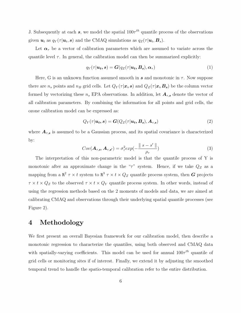
J. Subsequently at each s, we model the spatial 100τ th quantile process of the observations
given ut as qY (τ |ut, s) and the CMAQ simulations as qZ(τ |ut,Bs).
Let ατ be a vector of calibration parameters which are assumed to variate across the
quantile level τ . In general, the calibration model can then be summarized explicitly:
qY (τ |ut, s) = G(qZ(τ |ut, Bs),ατ ) (1)
Here, G is an unknown function assumed smooth in s and monotonic in τ . Now suppose
there are ns points and nB grid cells. Let QY (τ |x, s) and QZ(τ |x,Bs) be the column vector
formed by vectorizing these ns EPA observations. In addition, let Aτ,s denote the vector of
all calibration parameters. By combining the information for all points and grid cells, the
ozone calibration model can be expressed as:
QY (τ |ut, s) = G(QZ(τ |ut, Bs),Aτ,s) (2)
where Aτ,s is assumed to be a Gaussian process, and its spatial covariance is characterized
by:
Cov(Aτ,s,Aτ,s′) = σ2τexp(−
‖ s− s′ ‖ρτ
) (3)
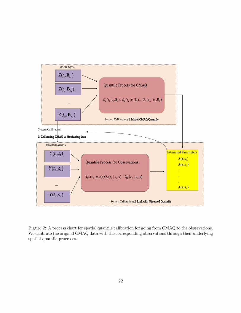
The interpretation of this non-parametric model is that the quantile process of Y is
monotonic after an approximate change in the “τ” system. Hence, if we take QZ as a
mapping from a R2 τ × t system to R3 τ × t×QZ quantile process system, then G projects
τ × t × QZ to the observed τ × t × QY quantile process system. In other words, instead of
using the regression methods based on the 2 moments of models and data, we are aimed at
calibrating CMAQ and observations through their underlying spatial quantile processes (see
Figure 2).
4 Methodology
We first present an overall Bayesian framework for our calibration model, then describe a
monotonic regression to characterize the quantiles, using both observed and CMAQ data
with spatially-varying coefficients. This model can be used for annual 100τ th quantile of
grid cells or monitoring sites if of interest. Finally, we extend it by adjusting the smoothed
temporal trend to handle the spatio-temporal calibration refer to the entire distribution.
6
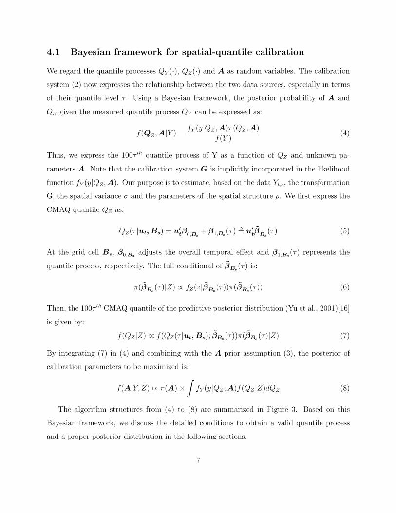
4.1 Bayesian framework for spatial-quantile calibration
We regard the quantile processes QY (·), QZ(·) and A as random variables. The calibration
system (2) now expresses the relationship between the two data sources, especially in terms
of their quantile level τ . Using a Bayesian framework, the posterior probability of A and
QZ given the measured quantile process QY can be expressed as:
f(QZ ,A|Y ) =fY (y|QZ ,A)π(QZ ,A)
f(Y )(4)
Thus, we express the 100τ th quantile process of Y as a function of QZ and unknown pa-
rameters A. Note that the calibration system G is implicitly incorporated in the likelihood
function fY (y|QZ ,A). Our purpose is to estimate, based on the data Yt,s, the transformation
G, the spatial variance σ and the parameters of the spatial structure ρ. We first express the
CMAQ quantile QZ as:
QZ(τ |ut, Bs) = u′tβ0,Bs
+ β1,Bs(τ) , u′
tβBs(τ) (5)
At the grid cell Bs, β0,Bsadjusts the overall temporal effect and β1,Bs
(τ) represents the
quantile process, respectively. The full conditional of βBs(τ) is:
π(βBs(τ)|Z) ∝ fZ(z|βBs
(τ))π(βBs(τ)) (6)
Then, the 100τ th CMAQ quantile of the predictive posterior distribution (Yu et al., 2001)[16]
is given by:
f(QZ |Z) ∝ f(QZ(τ |ut, Bs); βBs(τ))π(βBs(τ)|Z) (7)
By integrating (7) in (4) and combining with the A prior assumption (3), the posterior of
calibration parameters to be maximized is:
f(A|Y, Z) ∝ π(A)×∫fY (y|QZ ,A)f(QZ |Z)dQZ (8)
The algorithm structures from (4) to (8) are summarized in Figure 3. Based on this
Bayesian framework, we discuss the detailed conditions to obtain a valid quantile process
and a proper posterior distribution in the following sections.
7

4.2 System calibration and spatial quantile processes
Our model is motivated by a desire to improve the calibration strategy, especially correcting
outputs at extreme monitoring events. In this section, we briefly consider how the calibration
problem can be posed in the above Bayesian framework, particularly, how to determine
likelihood of both CMAQ and observed data via QZ(τ |ut, Bs) and G(QZ(τ |ut, Bs),Aτ,s).
4.2.1 Spatial-quantile process for CMAQ
In general, all the points s falling in the same 12 km square region are assigned the same
CMAQ output value. However, the model outputs and the observations are incomparable
due to such different spatial scales. Therefore, we link the spatial process in the model to a
point level process before using it for calibration. We model the quantile function from the
CMAQ models as follows:
QZ(τ |Bs) = β(τ,Bs) (9)
where the parameter function β(τ,Bs) are the spatially-varying coefficients for the 100τ th
quantile level.
Because QZ(τ) is nondecreasing in τ given a grid cell Bs, the process β(τ,Bs) must be
constructed as a monotonic function as:
β(τ,Bs) = I(τ)′β(Bs) = β0(Bs) +M∑m=1
Im(τ)βm(Bs) (10)
To achieve the monotonic properties, truncate power functions and polynomial basis func-
tions are widely used in the recent literature ( Cai et al., 2007; Reich et al., 2010)[17][12].
For instance, Berstein basis polynomials Im(τ) =
(Mm
)τm(1− τ)M−m reduces the compli-
cated monotonicity constraints to a sequence of simple constraints βm − βm−1 ≥ 0, for m =
2, ..., M (Reich et al.(2010))[12]. However, polynomials do have a limitation: changing the
behavior of β(τ,Bs) near one value τ1 has radical implications for its behavior for any other
value τ2. Thus, when M is small, the polynomial transformation which is satisfactory for the
central portion of the distribution, might exhibit unpleasing features in the tails (Ramsay,
1988)[18]. Choosing a large M helps but the computing burden becomes heavy. This poses
8

the problem of how to retain flexibility, while leaving the function elsewhere constrained as
desired.
In this paper, we model the function I using monotone spline regression by piece-
wise polynomials. In particular, we focus on the integrated splines Im, or I-splines for
the sake of brevity (Ramsay J. O., 1988; John Lu et al.)[18][19]. For a simple knot se-
quence {γ1, ..., γM+h}, M is the number of free parameters that specify the spline function
having the specified continuity characteristics, and h is the degree of piecewise polyno-
mial Im. For all τ , there exists m such that γm ≤ τ < γm+1. For application to the
important case where k=3, let: I∗1 ,(τ − γm)
(γm+2 − γm+1); I∗2 ,
(τ − γm+1)2 − (γm+3 − τ)2
(γm+3 − γm+1)(γm+2 − γm+1);
I∗3 ,(γm+3 − τ)3
(γm+3 − γm+1)(γm+3 − γm)(γm+2 − γm+1)− (τ − γm)3
(γm+3 − γm)(γm+2 − γm)(γm+2 − γm+1).
The I-spline Im will be piecewise cubic, zero for τ < γm and unity for τ ≥ γm+3, with
the direct expressions:
Im(τ |γ) =
0, if τ < γm(τ − γm)3
(γm+1 − γm)(γm+2 − γm)(γm+3 − γm), if γm ≤ τ < γm+1
I∗1 + I∗2 + I∗3 , if γm+1 ≤ τ < γm+2
1− (γm+3 − τ)3
(γm+3 − γm+2)(γm+3 − γm+1)(γm+3 − γm), if γm+2 ≤ τ < γm+3
1, if τ ≥ γm+3
(11)
As the I-spline is an integral of nonnegative splines, this provides a set of which, when
combined with nonnegative values of the coefficients βm(Bs), yields monotone splinesM∑m=1
Im(τ)βm(Bs).
To ensure the quantile constraint, we introduce latent unconstrained variable βm(Bs)∗
and take:
βm(Bs) =
{βm(Bs)
∗ if βm(Bs)∗ ≥ 0
0 otherwise(12)
Therefore a model using β(Bs) induces via (10) a quantile process of QZ(τ |Bs). Without
loss of generality, we choose the knots series within γ1 = 0 and γM+h = 1. The quantile
process thus satisfies the boundary conditions:
QZ(0|Bs) = β0(Bs) = Lz(Bs), QZ(1|Bs) = β0(Bs) +M∑m=1
βm(Bs) = Uz(Bs) (13)
9

where [Lz(Bs), Uz(Bs)] gives the range of Z over the grid cell Bs in formula (9). Here,
we rescale CMAQ data on themselves at each grid cell, thus Lz(Bs) ≡ 0 and Uz(Bs) ≡
1. In addition, assuming βm(Bs)∗ have prior βm(Bs)
∗ ∼ N(βm,Σm), with Σm
(Bs,B′s) =
σ2mBexp(−||s− s′||/ρmB
). The full conditional distribution of π(βm(Bs)|Z) are then given
by f(Z|βm(Bs), βm(Bs)∗)π(βm(Bs)| βm(Bs)
∗)π(βm(Bs)∗). Subsequently, the predictive
posterior distribution f(QZ(τ,Bs)|Z) of the the 100τ th CMAQ quantile is obtained by (7).
4.2.2 Spatial-quantile calibration : from CMAQ to monitoring processes
For the purpose of calibrating spatial-quantile process, we make use of monotonically in-
creasing map ηs drawing from the CMAQ predictive posterior distribution:
ηs(τ)d= f(QZ |Z) ∝ f(QZ(τ |Bs); βBs(τ))π(βBs(τ)|Z) (14)
Thus we have the observed quantiles of Y as follows:
QY (τ |Z, s) = I(ηs(τ))′α(s) = α0(s) +M∑m=1
Im(ηs(τ))αm(s) (15)
α(s) are spatially-varying coefficients. Similar as equation (12), we introduce a latent un-
constrained variable αm(s)∗ to ensure the quantile constraints:
αm(s) =
{αm(s)∗ if αm(s)∗ ≥ 0
0 otherwise(16)
αm(s)∗ are modeled as multivariate mean-zero Gaussian spatial process with boundary con-
ditions:
QY (0|Z, s) = α0(s) = Ly(s), QY (1|Z, s) = α0(s) +M∑m=1
αm(s) = Uy(s) (17)
where (Ly(s), Uy(s)) are the range of Y given location s. However, strict bounds on Y may
not be known a priori. To satisfy that the posterior has a proper distribution (see appendix),
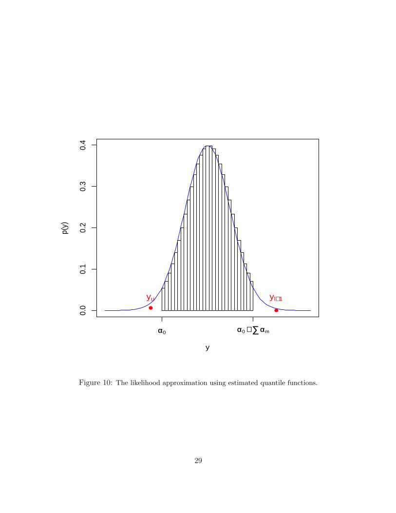
we take a truncate likelihood:
f ∗Y (y|QY ) = {e−ωL(α0 − y)}1(y < α0)
× {e−ωU(y − (α0 +∑
αm)))}1(y > α0 +∑
αm)
× {fY (y|Z, s)}1(α0 ≤ y ≤ α0 +∑
αm)(18)
10

where ωL, ωU are known positive rate parameters and fY (y|Z, s) is the density function
derived from both the CMAQ and observed quantile functions, and its computing algorithm
is provided in Section 4.2.3. The resulting likelihood has an exponential decay once the esti-
mated quantile boundaries do not include certain observed values. Also, we assume that there
exist (M+1) mean-zero unit-variance independent Gaussian processes α0(s), α1(s), ..., αM(s)
such that, cov(αm(s), αm(s′)) = σ2msexp(−||s− s′||/ρms) and ρms is the spatial decay pa-
rameter for Gaussian process αm(s), m=0,1,...,M.
4.2.3 Model fitting : likelihood approximations using calibrated quantiles
In this section, we focus on discussing how to obtain Y’s likelihood only based on its quantile
process QY (τ |Z, s) = I(ηs(τ))′α(s) and CMAQ predictive quantile ηs(τ). Suppose the
constraints (12) and (16) are satisfied, then τ → QY (τ |Z, s) is monotonically increasing.
Hence, the process (15) uniquely determines a unconditional sampling density for Y in the
form (Tokdar et al. 2010)[11]:
fY (y|Z, s) =1
∂∂τQY (τ |Z, s)
|τ=τZ,s(y) (19)
where τZ,s(y) is the solution y = QY (τ |Z, s) in τ , and we apply the truncated likelihood
(18) to approximate the density function:
f ∗Y (y|QY (Z, s), ηs(τZ,s)) = {e−ωL(α0 − y)}1(y < α0)
×{e−ωU(y − (α0 +∑
αm)))}1(y > α0 +∑
αm)
×{ 1
∂∂τQY (τ |Z, s)
|τ=τZ,s(y)}1(α0 ≤ y ≤ α0 +
∑αm)
(20)
when α0 ≤ y ≤ α0 +∑
αm, the partial log-likelihood function of fY (y|Z, s), over the
monotonicity restrictions of (ηs, α(s)) is defined as:∑i
log fY (yi|s) = −∑i
log∂
∂τQY (τ |s) |τ=τZ,s(yi)
= −∑i
log∂QY (τ |s)∂ηs(τ)
· ∂ηs(τ)
∂τ|τ=τZ,s(yi) (21)
11

where τZ,s(yi) solves yi = QY (τ |Z, s), i = 1,2,...,n. A solution τZ,s(y) to QY (τ |Z, s)− y = 0
can be efficiently obtained using Newton’s Recursion:
τ(k+1)Z,s (y) = τ
(k)Z,s(y)− QY (τ |Z, s)− y
∂∂τQY (τ
(k)Z,s(y)|Z, s)
, (22)
where τ(0)Z,s is an initial value in [0, 1], and we choose the lower bound of an estimated quantile
interval where y lies in our practice. The evaluations of QY (τ |Z, s) and∂
∂τQY (τ |Z, s) at
various values of τ ∈ [0, 1] can be done by:
∂
∂τQY (τ |Z, s) =
∂
∂ηs
QY (τ |Z, s) · ∂∂τηs
= {M∑m=1
∂
∂ηs
Im(ηs(τZ,s(y)))αm(s)} · {M∑m=1
∂
∂τIm(τZ,s(y))βm(s)} (23)
To simplify the notation, letD∗1 =3
(γm+2 − γm+1); D∗2 =
−3(γm+3 − η)2
(γm+3 − γm+1)(γm+3 − γm)(γm+2 − γm+1)
+−3(η − γm)2
(γm+3 − γm)(γm+2 − γm)(γm+2 − γm+1). Then the derivative of I-spline,
∂
∂ηIm(η(·)) con-
sists of straightline segments as follows
∂
∂ηIm(η|γ) =
0, if η < γm3(η − γm)2
(γm+1 − γm)(γm+2 − γm)(γm+3 − γm), if γm ≤ η < γm+1
D∗1 +D∗2, if γm+1 ≤ η < γm+2
3(γm+3 − η)2
(γm+3 − γm+2)(γm+3 − γm+1)(γm+3 − γm), if γm+2 ≤ η < γm+3
0, if η ≥ γm+3
(24)
The steps given in equations (21) and (24) provide a fast algorithm to compute the likelihood
at any given value of the parameter η (Tokdar et al., 2010)[11]. Using Markov Chain Monte
Carlo (MCMC), the posterior distributions are summarized subsequently by evaluating the
likelihood (20) and CMAQ distribution (14).
4.3 Spatial-temporal quantile calibration
The calibration model in section 4.2 can be extended to accommodate data collected over
space and time. If we denote time with t, t=1,2,...,T, ut=(ut1, ut2, ..., utJ)′. ut1 ≡ 1 and utj
12
is the B-spline of t with df=J-1, j=2,...,J. Then QY (τ |ut, s) denotes the τ th quantiles process
of observed daily 8-hour maximum ozone concentration at s and time t, while QZ(τ |ut, Bs)
is the τ th CMAQ quantile levels for grid cell Bs given time t. Again, we relate the 12 km
CMAQ grid cell Bs to each monitoring site s.
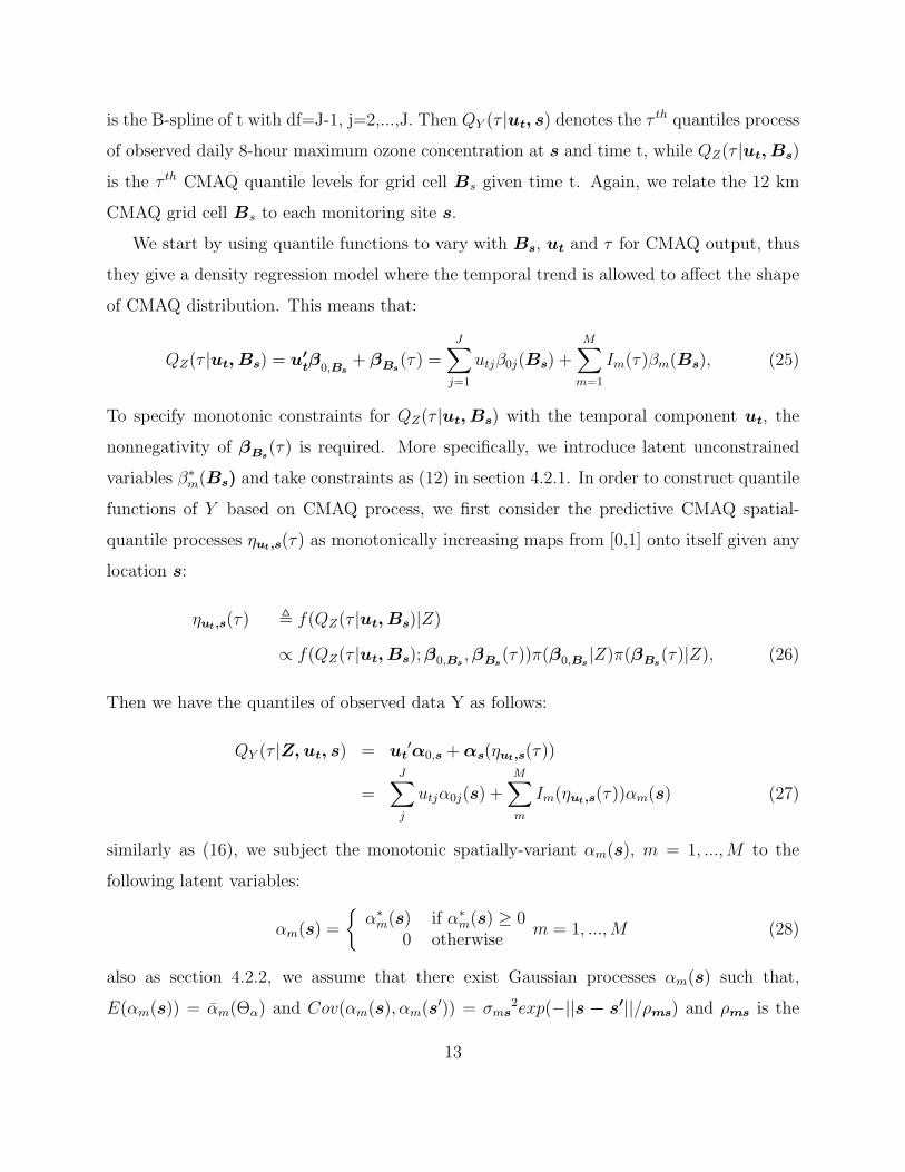
We start by using quantile functions to vary with Bs, ut and τ for CMAQ output, thus
they give a density regression model where the temporal trend is allowed to affect the shape
of CMAQ distribution. This means that:
QZ(τ |ut, Bs) = u′tβ0,Bs
+ βBs(τ) =
J∑j=1
utjβ0j(Bs) +M∑m=1
Im(τ)βm(Bs), (25)
To specify monotonic constraints for QZ(τ |ut, Bs) with the temporal component ut, the
nonnegativity of βBs(τ) is required. More specifically, we introduce latent unconstrained
variables β∗m(Bs) and take constraints as (12) in section 4.2.1. In order to construct quantile
functions of Y based on CMAQ process, we first consider the predictive CMAQ spatial-
quantile processes ηut,s(τ) as monotonically increasing maps from [0,1] onto itself given any
location s:
ηut,s(τ) , f(QZ(τ |ut, Bs)|Z)
∝ f(QZ(τ |ut, Bs);β0,Bs,βBs
(τ))π(β0,Bs|Z)π(βBs
(τ)|Z), (26)
Then we have the quantiles of observed data Y as follows:
QY (τ |Z, ut, s) = ut′α0,s +αs(ηut,s(τ))
=J∑j
utjα0j(s) +M∑m
Im(ηut,s(τ))αm(s) (27)
similarly as (16), we subject the monotonic spatially-variant αm(s), m = 1, ...,M to the
following latent variables:
αm(s) =
{α∗m(s) if α∗m(s) ≥ 0
0 otherwisem = 1, ...,M (28)
also as section 4.2.2, we assume that there exist Gaussian processes αm(s) such that,
E(αm(s)) = αm(Θα) and Cov(αm(s), αm(s′)) = σms2exp(−||s− s′||/ρms) and ρms is the
13
spatial decay parameter for Gaussian process αm(s). The different temporal trends between
CMAQ and observed quantile process are then adjusted through the calibration parameters
α0(s), α1(s), ..., αm(s).
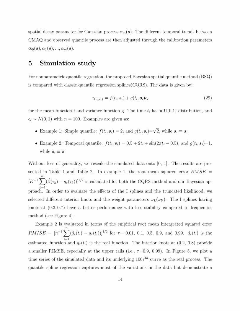
5 Simulation study
For nonparametric quantile regression, the proposed Bayesian spatial quantile method (BSQ)
is compared with classic quantile regression splines(CQRS). The data is given by:
z(ti,si) = f(ti, si) + g(ti, si)εi (29)
for the mean function f and variance function g. The time ti has a U(0,1) distribution, and
εi ∼ N(0, 1) with n = 100. Examples are given as:
• Example 1: Simple quantile: f(ti, si) = 2, and g(ti, si)=√
2, while si ≡ s.
• Example 2: Temporal quantile: f(ti, si) = 0.5 + 2ti + sin(2πti − 0.5), and g(ti, si)=1,
while si ≡ s.
Without loss of generality, we rescale the simulated data onto [0, 1]. The results are pre-
sented in Table 1 and Table 2. In example 1, the root mean squared error RMSE =
[K−1
K∑k=1
(β(τk) − qz(τk))]1/2 is calculated for both the CQRS method and our Bayesian ap-
proach. In order to evaluate the effects of the I splines and the truncated likelihood, we
selected different interior knots and the weight parameters ωL(ωU). The I splines having
knots at (0.3, 0.7) have a better performance with less stability compared to frequentist
method (see Figure 4).
Example 2 is evaluated in terms of the empirical root mean intergrated squared error
RMISE = [n−1
n∑i=1
(qτ (ti) − qτ (ti))]1/2 for τ= 0.01, 0.1, 0.5, 0.9, and 0.99. qτ (ti) is the
estimated function and qτ (ti) is the real function. The interior knots at (0.2, 0.8) provide
a smaller RIMSE, especially at the upper tails (i.e., τ=0.9, 0.99). In Figure 5, we plot a
time series of the simulated data and its underlying 100τ th curve as the real process. The
quantile spline regression captures most of the variations in the data but demonstrate a
14
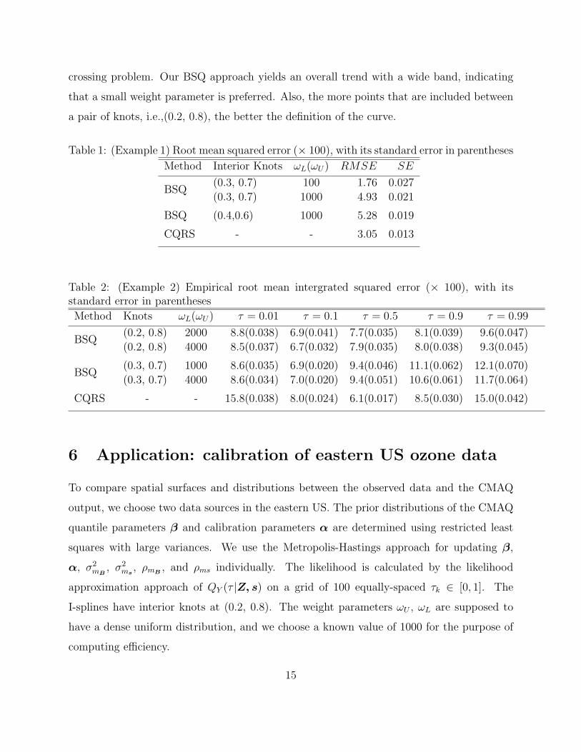
crossing problem. Our BSQ approach yields an overall trend with a wide band, indicating
that a small weight parameter is preferred. Also, the more points that are included between
a pair of knots, i.e.,(0.2, 0.8), the better the definition of the curve.
Table 1: (Example 1) Root mean squared error (× 100), with its standard error in parentheses
Method Interior Knots ωL(ωU) RMSE SE
(0.3, 0.7) 100 1.76 0.027BSQ
(0.3, 0.7) 1000 4.93 0.021
BSQ (0.4,0.6) 1000 5.28 0.019
CQRS - - 3.05 0.013
Table 2: (Example 2) Empirical root mean intergrated squared error (× 100), with itsstandard error in parentheses
Method Knots ωL(ωU) τ = 0.01 τ = 0.1 τ = 0.5 τ = 0.9 τ = 0.99
(0.2, 0.8) 2000 8.8(0.038) 6.9(0.041) 7.7(0.035) 8.1(0.039) 9.6(0.047)BSQ
(0.2, 0.8) 4000 8.5(0.037) 6.7(0.032) 7.9(0.035) 8.0(0.038) 9.3(0.045)
(0.3, 0.7) 1000 8.6(0.035) 6.9(0.020) 9.4(0.046) 11.1(0.062) 12.1(0.070)BSQ
(0.3, 0.7) 4000 8.6(0.034) 7.0(0.020) 9.4(0.051) 10.6(0.061) 11.7(0.064)
CQRS - - 15.8(0.038) 8.0(0.024) 6.1(0.017) 8.5(0.030) 15.0(0.042)
6 Application: calibration of eastern US ozone data
To compare spatial surfaces and distributions between the observed data and the CMAQ
output, we choose two data sources in the eastern US. The prior distributions of the CMAQ
quantile parameters β and calibration parameters α are determined using restricted least
squares with large variances. We use the Metropolis-Hastings approach for updating β,
α, σ2mB
, σ2ms
, ρmB, and ρms individually. The likelihood is calculated by the likelihood
approximation approach of QY (τ |Z, s) on a grid of 100 equally-spaced τk ∈ [0, 1]. The
I-splines have interior knots at (0.2, 0.8). The weight parameters ωU , ωL are supposed to
have a dense uniform distribution, and we choose a known value of 1000 for the purpose of
computing efficiency.
15

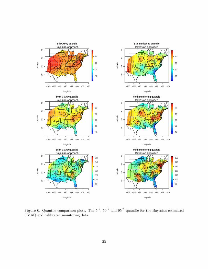
The estimated CMAQ quantile and its calibration for monitoring data are plotted in
Figure 6. Both of the two spatial-quantile processes are obtained by our Bayesian algorithm.
At τ= 0.05, 0.5, and 0.95, the empirical root mean integraded squared error RMISE =
[n−1
n∑i=1
(qzτ (si)− qyτ (si))]1/2 is calculated. The RMISE at the 50th quantile is equal to 7.13,
while the value is 13.17 for the 5th percentile and 15.46 for the 95th percentile, respectively.
The results show agreement between the distributions of CMAQ output and the monitoring
data at their median level, but show large differences for the tails. Also, from the contour
plot, we conclude that the CMAQ data are smoother than the observed spatial structure,
indicating that the physically based numerical models can not capture both the extreme
values and spatial correlations that are in the monitoring data.
Due to these differences, it is critical to calibrate the CMAQ data considering its spatial-
quantile structure. Based on the estimated CMAQ-monitoring calibration model, a nonlinear
transformation is made to the CMAQ data using G(Zt,s, A(τ, s)) = α0 +M∑m
Im(Zt,s)αm,
where α are the posterior estimations. Then we rescale G(Zt,s, A(τ, s)) to its original
range. Because G is a monotonic function, the quantiles of G(Zt,s,A(τ, s)) are equal to
G(QZ(τ |s),A(τ, s)) = QY (τ |s). We calculate qM(τk, s) (the sample quantiles of the mon-
itoring data), qC(τk, s) (the quantiles of the Bayesian calibrated data) and qL(τk, s) (the
quantiles from the linear regression model), at τk ∈ [0.01, 0.97] and location s. The root
mean squared error RMSE(qM , q|s) = [K−1
K∑k=1
(qM(τk, s) − q(τk, s))]1/2 is calculated for
both linear regression method and our Bayesian approach at each location s. Figure 7 shows
maps of the above quantiles when τ = 0.95, and the difference root mean squared error
DRMSE = (RMSE(qM , qC |s) −RMSE( ˆqM , qL|s)) /RMSE( ˆqM , qL|s) between the linear
regression method and the quantile calibration method. The differences range from -77%
to 66%, and is -30% on average. The results show that 57 out of 68 (83.8%) sites have a
reduced RMSE using the Bayesian calibration method. As we expected, the performance of
the calibrated CMAQ model data is consistent with the performance of the monitoring data
in terms of the quantile level τ .
16

7 Discussion
In this paper, we propose a Bayesian spatial quantile calibration model for adjusting the
behavior between CMAQ model output and monitoring data. Particularly, we focus on
calibrating the extreme values. Thus, instead of using the default approach based on the
first two moments of the models and data, we calibrated the two data sources through their
underlying quantile processes. We investigated two quantile processes: (1) estimated spatial-
quantiles for CMAQ; (2) the predicted monitoring quantiles based on CMAQ calibrations.
We conclude that the CMAQ and monitoring data are similar around their median values,
but present large differences at the upper and lower tails over eastern US. The investigated
transformation between CMAQ and the observed quantile process is then applied to model
output data, resulting in a calibrated series whose spatial and quantile structure is consistent
with the monitoring data.
Due to the different spatial scales of the CMAQ output and the observations, we as-
sume that both the CMAQ and observed quantile processes have a spatial structure with
exponential decay parameters. This assumption is made to obtain computing efficiency.
More complicated spatial processes, i.e., conditional autoregressive (CAR) model for grid-
ded CMAQ data, and spatial linear coregionalization models for calibrating spatial quantiles,
will be considered in future work.
Also, temporal components, known to be an important factor for ozone trend, play less of
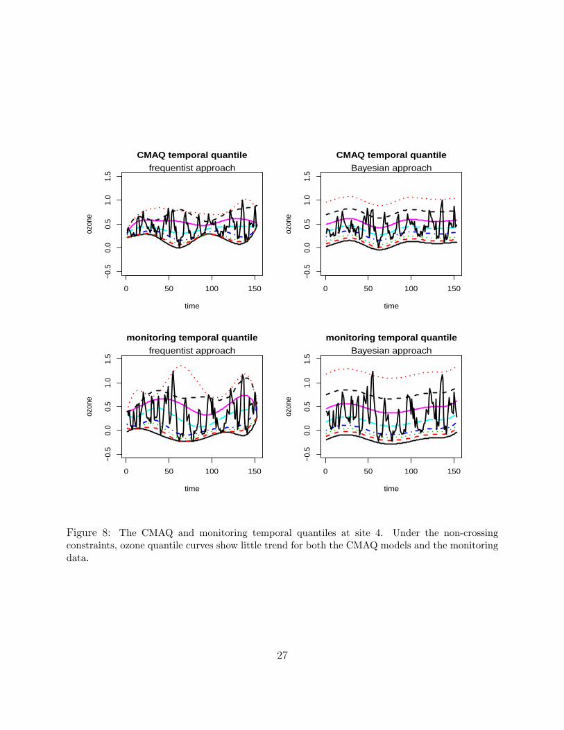
a role when taking both quantile and spatial structure into account (see Figure 8). Another
approach is to consider the smoothing spline as a covariate, then evaluate its effect on
the conditional distributions (see Figure 9 for the individual quantile surfaces for both the
CMAQ data and monitoring data at a specific site); however, the quantile calibrations, as
a tranformations of one quantile process to another simultaneously, require a valid quantile
process with the non-crossing and monotonic constraints. An efficient way to calibrate this
type of spatial-temporal-quantile surface simultaneously is another avenue for future work.
17

8 Appendix
If the likelihood is given by fomula (18) and p(α) ∝ 1, then the posterior distribution of α,
π(α|Y ), will have a proper distribution. In other words:
0 <
∫π(α|Y )dα <∞ (30)
Proof. Suppose y(1) ≤ y(2)... ≤ y(n), and both ωL and ωU are two finite positive numbers.
We first consider two extreme situations:
(1) yi < α0, for all yi, i=1, 2,..., n. Hence, we have y(n) < α0 and:∫π(α|Y )dα =
∫ n∏i=1
fY (yi|(α)π(α)dα ∝∫{α0≥y(n)}
exp{−∑i
ωL(α0 − yi)}dα
∝∫{α0≥y(n)}
exp{−nωL(α0 − y)}dα
∝ 1
nωLexp{−nωL(y(n) − y)}
∈ (0,∞) (31)
(2) Another situation is: yi > α0 +∑
αm, for all yi, i=1, 2,..., n. As a result, we have
y(1) > α0 +∑
αm and:
∫π(α|Y )dα =
∫ n∏i=1
fY (yi|(α)π(α)dα
∝∫{α0+
∑m αm≤y(1)}
exp{−∑i
ωU(yi − (α0 +∑m
αm))}dα
∝∫{α0+
∑m αm≤y(1)}
exp{−nωU(y − (α0 +∑m
αm)}dα
∝ 1
nωUexp{−nωU(y − y(1))}
∈ (0,∞) (32)
In general, suppose y(1)..., y(u)< α0 ≤ y(u+1)...≤ y(l) ≤ α0 +∑m
αm <y(l+1)..., y(n) (see
18

Figure 10), then we have:∫π(α|Y )dα ∝ 1
uωUexp{−ωU(uy(u) −
u∑i=1
y(i))}
× 1
(n− l)ωLexp{−ωL(
n∑i=l+1
y(i) − (n− l)y(l+1))}
×∫ l
i=u+1
{ 1
∂∂τQY (τ)
|τ=τ(y(i))}dα
∈ (0,∞) (33)
The statement is proved.
References
[1] M. Kennedy and A. O’Hagan, “Bayesian calibration of computer models,” Journal of theRoyal Statistical Society: Series B (Statistical Methodology), vol. 63, no. 3, pp. 425–464,2001.
[2] C. Paciorek, “Combining spatial information sources while accounting for systematicerrors in proxies,” Journal of the Royal Statistical Society, 2000.
[3] M. Fuentes and A. E. Raftery, “Model evaluation and spatial interpolation by bayesiancombination of observations with outputs from numerical models,” Biometrics, vol. 61,no. 1, pp. 36–45, 2005.
[4] C. Y. Lim, M. Stein, J. K. Ching, and R. Tang, “Statistical properties of differencesbetween low and high resolution cmaq runs with matched initial and boundary condi-tions,” Environmental Modelling and Software, no. 25(1), pp. 158–169, 2010.
[5] B. K. Eder and S. Yu, “A performance evaluation of the 2004 release of models-3 cmaq,”Air Pollution Modeling and Its Application XVII, no. 6, pp. 534–542, 2007.
[6] V. J. Berrocal, A. E. Gelfand, and D. M. Holland, “A spatio-temporal downscaler foroutput from numerical models,” Journal of Agricultural, Biological, and EnvironmentalStatistics, vol. 15, pp. 176–197, 2010.
[7] R.Koenker, Quantile Regression. Econometric Society Monograph Series, CambridgeU. Press, 2005.
[8] H. Kozumi and G. Kobayashi, “Gibbs sampling methods for bayesian quantile regres-sion,” Journal of Statistical Computation and Simulation, 2011.
19
[9] Y. Wu and Y. Liu, “Stepwise multiple quantile regression estimation,” Statistics andIts Interface, vol. 2, 2009.
[10] H. D. Bondell, B. J. Reich, and H. Wang, “Non-crossing quantil regression curve esti-mation,” Biometrika, vol. 97, 2010.
[11] S. Tokdar and J. Kadane, “Simultaneous linear quantile regression: A semiparametricbayesian approach.,” In press, 2010.
[12] B. J. Reich, M. Fuentes, and D. Dunson, “Bayesian spatial quantile regression,” Journalof the American Statistical Association, vol. In press, 2010.
[13] M. Lavine, “On an approximate likelihood for quantiles,” Biometrika, vol. 82, 1995.
[14] D. B. Dunson and J. A. Taylor, “Approximate bayesian inference for quantiles,” Journalof Nonparametric Statistics, vol. 17, 2005.
[15] D. Byun and K. L. Schere, “Review of the governing equations, computational algo-rithms, and other components of the models-3 community multscale air quality (cmaq)modeling system,” Appl. Mech. Rev., 2006.
[16] K. Yu and R. A. Moyeed, “Bayesian quantile regression,” Statistics & Probability Letters,vol. 54, no. 4, pp. 437 – 447, 2001.
[17] B. Cai and D. B. Dunson, “Bayesian multivariate isotonic regression splines:applicationsto carcinogenicity studies,” Journal of the American Statistical Association, vol. 102,pp. 1158–1171, 2007.
[18] J. O. Ramsay, “Regression splines in action,” Statistical Science, vol. 3, pp. 425–441,1988.
[19] Z. Q. J. Lu and D. B. Clarkson, “Monotone spline and multidimensional scaling,”http://www.reocities.com/zqjlu/asa2.pdf.
20

−105 −95 −90 −85 −80 −75 −70
30
35
40
45
Longitude
La
titu
de
60
70
80
90
100
*
CMAQ 90th quantilefrequentist approach
−105 −95 −90 −85 −80 −75 −70
30
35
40
45
Longitude
La
titu
de
60
70
80
90
100
*
Monitoring 90th quantilefrequentist approach
Histogram of CMAQ ozone
De
nsi
ty
30 40 50 60 70 80 90
0.0
00
.02
0.0
4
Histogram of monitoring ozone
De
nsi
ty
20 40 60 80 100 120
0.0
00
0.0
10
0.0
20
0 50 100 150
0.0
00
0.0
15
0.0
30
Density comparison
De
nsi
ty
CMAQMonitorming data
0.0 0.2 0.4 0.6 0.8 1.0
40
60
80
10
0
Sample quantile
Tau1
ozo
ne
CMAQMonitorming data
Figure 1: Maps of the sample 90th quantile levels of the ozone concentration; the ” ∗ ” representsa randomly selected (i.e., 59th) monitoring site. We draw the maps for both observed and CMAQdata to identify their differences.
21
MODEL DATA
…
System Calibration: 1. Model CMAQ Quantile
MONITORING DATA
…
System Calibration: 2. Link with Observed Quantile
Quantile Process for CMAQ
),|( 1 sBtZ uQ , ),|( 2 sBtZ uQ … ),|( sBtKZ uQ
),( 11 stY
),( 22 stY
),( nn stY
Quantile Process for Observations
),|( 1 stY uQ , ),|( 2 stY uQ … ),|( stKY uQ
)(
.
.
.
)(
)(
2
1
nsτ,Α
sτ,Α
sτ,Α
Estimated Parameters
System Calibration:
3. Calibrating CMAQ to Monitoring data
),( 1 1sBtZ
),( 2 2sBtZ
),(nsBntZ
Figure 2: A process chart for spatial quantile calibration for going from CMAQ to the observations.We calibrate the original CMAQ data with the corresponding observations through their underlyingspatial-quantile processes.
22

Spatial – quantile process for CMAQ
0
1
( | ) ( ) ( ) ( )M
Z m m
m
Q s s I s
mI : Monotonic I spline;
Spatially variant coefficients β(s) for CMAQ ( | )ZQ s ;
Likelihood approximation by ( | )ZQ s ;
,A ( s) : Monotonic
mapping from ( | )s Z
to
( | )Q sY
Spatial – quantile process for monitoring data
0
1
( | ) ( ) ( ( | )) ( )M
m m
m
Q s s I s s
Y Z
Spatially variant calibration parameters α(s) ;
Likelihood approximation by predictive CMAQ
( | )s Z and monitoring quantile ( | )Q sY .
( | )s Z: Predictive
posterior quantile for
CMAQ
Figure 3: The Bayesian framework for the spatial-quantile calibration approach. The left andmiddle panels present CMAQ quantile and monitoring quantile estimates at the 59th site. The rightpanel provides the 90th ozone quantile over the eastern U.S. using our Bayesian spatial quantilecalibration method.
23

−0.2 0.0 0.2 0.4 0.6 0.8 1.0 1.2
0.0
0.5
1.0
1.5
2.0
2.5
3.0
Density
De
nsi
ty
●
●●
●
●
●
●
●
●
●
●
●
●
●
●
● ●
●
●
●
●
●
●
●
●
●
●
●
●
●
●
●●
●
●
●
●
●
●
●
●
●●
●
●
●
●
●
●
●●
●
●●
●
●
●
●
●
●
●
●
●●
●
●●
●
●
●
●
●
●
●
●
●
●
●
●
●●
●
●
●
●
●
●●
●
●
●
●
●
●
●
●
●
●●
●
Figure 4: Simulation results for the simple quantile functions in Example 1. Interior knots areplaced at 0.15, 0.8 with a weight parameter equal to 100.
0.0 0.2 0.4 0.6 0.8 1.0
−0.2
0.2
0.6
1.0
CQRS
time
0.0 0.2 0.4 0.6 0.8 1.0
−0.2
0.2
0.6
1.0
Real process
time
0.0 0.2 0.4 0.6 0.8 1.0
−0.2
0.2
0.6
1.0
BSQ
time
0.0 0.2 0.4 0.6 0.8 1.0
0.0
0.2
0.4
0.6
0.8
1.0
Simulated data
time
y
Figure 5: Bayesian nonparametric quantile (BSQ) regression from Example 2. Interior knots areplaced at 0.2, 0.8 with weight parameter equal to 2000. We add a sin function to mimic the temporaltrend in reality. The classic quantile regression spline (CQRS) has crossed quantile curves, whichviolate the concept of a valid quantile process.
24
−105 −100 −95 −90 −85 −80 −75 −70
30
35
40
45
Longitude
La
titu
de
10
20
30
40
34
36
36
38
38
38
40
40
40
40
42
42
42
42
44
44
46 48
5 th CMAQ quantileBayesian approach
−105 −100 −95 −90 −85 −80 −75 −70
30
35
40
45
Longitude
La
titu
de
10
20
30
40
10
20
20
25
25
25
30
30 30
30
30
35
35 35
35
35
40
45
5 th monitoring quantileBayesian approach
−105 −100 −95 −90 −85 −80 −75 −70
30
35
40
45
Longitude
La
titu
de
40
50
60
70
80
55 60
60
60
65
65
65
65
70
70
70
75
75
75
80
50 th CMAQ quantileBayesian approach
−105 −100 −95 −90 −85 −80 −75 −70
30
35
40
45
Longitude
La
titu
de
40
50
60
70
80
45
50
55 60
60
60
60 60
65
65
70
70
75
75
75
80
50 th monitoring quantileBayesian approach
−105 −100 −95 −90 −85 −80 −75 −70
30
35
40
45
Longitude
La
titu
de
90
100
110
120
130
140
150
100 105
105 105
110
110
115
115
115
115
120
120
120
120
125
95 th CMAQ quantileBayesian approach
−105 −100 −95 −90 −85 −80 −75 −70
30
35
40
45
Longitude
La
titu
de
90
100
110
120
130
140
150
95
100
105
105
110
110
115
115 120
120
120
125 125
125
130
130 130 130
135
135
140
95 th monitoring quantileBayesian approach
Figure 6: Quantile comparison plots. The 5th, 50th and 95th quantile for the Bayesian estimatedCMAQ and calibrated monitoring data.
25

−105 −95 −90 −85 −80 −75 −70
3035
4045
Longitude
Latit
ude
60
80
100
120
140 90
90
90
100
100
110 110
120
120
120
130
95 th monitoring quantileFrequentist approach
−105 −95 −90 −85 −80 −75 −70
3035
4045
LongitudeLa
titud
e
60
80
100
120
140
80
90
90
100
100
110
110 120
120
120
120
130
130
130
130
140
140
95 th monitoring quantileBayesian approach
−105 −95 −90 −85 −80 −75 −70
3035
4045
Longitude
Latit
ude
60
80
100
120
140
80
90
90
100
100 110 110
110
110
120
120
120
130
130
95 th monitoring quantileLinear regression approach
−105 −95 −90 −85 −80 −75 −70
3035
4045
Longitude
Latit
ude
−0.8
−0.6
−0.4
−0.2
0.0
0.2
0.4
DRMSE between Bayesian and linear regression
Figure 7: The 95th quantile for the monitoring data, using both the quantile calibration and linearregression method. We compare the differences between the linear regression and the Bayesianquantile calibration methods in terms of the RMSE.
26
0 50 100 150
−0.5
0.0
0.5
1.0
1.5
CMAQ temporal quantile
time
ozon
e
frequentist approach
0 50 100 150
−0.5
0.0
0.5
1.0
1.5
CMAQ temporal quantile
time
ozon
e
Bayesian approach
0 50 100 150
−0.5
0.0
0.5
1.0
1.5
monitoring temporal quantile
time
ozon
e
frequentist approach
0 50 100 150
−0.5
0.0
0.5
1.0
1.5
monitoring temporal quantile
time
ozon
e
Bayesian approach
Figure 8: The CMAQ and monitoring temporal quantiles at site 4. Under the non-crossingconstraints, ozone quantile curves show little trend for both the CMAQ models and the monitoringdata.
27

OBS.Quantile surface
Error using packet 1NAs are not allowed in subscripted assignments
0.2
0.4
0.6
0.8
1.0
OBS.Quantile surface
50 100 1500.20.4
0.60.8
0
20
40
60
80
100
120
t
τ
Q(y)
0
20
40
60
80
100
120
CMAQ.Quantile surface
50 100 1500.20.4
0.60.8
0
20
40
60
80
100
120
t
τ
Q(y)
20
40
60
80
100
Figure 9: Temporal quantile surfaces at the 19th location for both the CMAQ data and Observeddata.
28
0.0
0.1
0.2
0.3
0.4
y
p(y)
αα0 αα0 ++ ∑∑ααm
●
yu
●
yl++1
Figure 10: The likelihood approximation using estimated quantile functions.
29