cardiff business school working paper series · 2017-02-07 · cardiff business school colum drive,...

Cardiff Economics Working Papers

Kent Matthews, Jianguang Guo and Nina Zhang

Non-Performing Loans and Productivity in Chinese Banks: 1997–2006

E2007/30

CARDIFF BUSINESS SCHOOL WORKING PAPER SERIES

This working paper is produced for discussion purpose only. These working papers are expected to be published in due course, in revised form, and should not be quoted or cited without the author’s written permission. Cardiff Economics Working Papers are available online from: http://www.cardiff.ac.uk/carbs/econ/workingpapers Enquiries: [email protected]

ISSN 1749-6101 November 2007

Cardiff Business School

Cardiff University Colum Drive

Cardiff CF10 3EU United Kingdom

t: +44 (0)29 2087 4000 f: +44 (0)29 2087 4419

www.cardiff.ac.uk/carbs

Non-Performing Loans and Productivity in Chinese Banks: 1997-2006

Kent Matthews*, Jianguang Guo**, and Nina Zhang**

*Cardiff Business School, Cardiff University, Wales

**Research Centre for Chinese Banking, CUFE Beijing

***Citibank (China) and Cardiff Business School

October 2007.

Abstract

This study examines the productivity growth of the nationwide banks of China over the ten years to 2006. Using a bootstrap method for the Malmquist index estimates of productivity growth are constructed with appropriate confidence intervals. The paper adjusts for the quality of the output by accounting for the non-performing loans on the balance sheets and test for the robustness of the results by examining alternative sets of outputs. The productivity growth of the state-owned banks is compared with the Joint-stock banks and it determinants evaluated. The paper finds that average productivity of the Chinese banks improved modestly over this period. Adjusting for the quality of loans, by treating NPLs as an undesirable output, the average productivity growth of the state-owned banks was zero or negative while productivity of the Joint-Stock banks was markedly higher. Keywords : Bank Efficiency, Productivity, Malmquist index, Bootstrapping JEL codes: D24, G21 Corresponding author: K Matthews

Cardiff Business School Colum Drive, Cardiff, CF10 3EU Wales, UK E-mail address: [email protected] Tel.: +44(0)292-875855

Paper prepared for the All China Economics International Conference 12-14 December 2007, City University of Hong Kong. We gratefully acknowledge the financial support of the British Academy SG-41928(IR) and Chinese Education Ministry projects for research on Humanity and Social Science No.04JZD0013. Comments welcome.

2

1. Introduction

Banking efficiency and banking reform is a vogue topic among Chinese

scholars. Banking sector reform in China, which has been a gradual and on-going

process since 1978, has provided Chinese researchers with ample material for the

study of efficiency dynamics in banking. A further stage of reform was announced in

1993 with the objective of creating an efficient and commercial banking sector.

Following the conditions of the WTO, in theory the Chinese banking market has been

open to foreign competition since the end of 2006. Chinese banks have also been

encouraged to allow foreign banks and investors to take minority shareholding

positions. The listing of three of the big four banks on the international exchange

during 2006-7 has been heralded as a financial success not only because of the

injection of foreign capital but also foreign managerial expertise to improve bank

management, performance and productivity. Given the acceptance strategic

investment by foreign banks in the smaller commercial banks; it is no surprise that

bank efficiency in China has become a popular topic of research in recent years.

There have been a number of studies of banking efficiency that have been

published in Chinese scholarly journals 1, but to date only a few studies are available

to non-Chinese readers2. The gradualist reforms of the banking sector and the

potential of foreign competition would be expected to improve efficiency and

productivity in the banking sector. Signs of improvement in the Chinese banking

sector have included improved profitability and declining non-performing loans and

objective evidence of improved performance has begun to emerge 3.

1 For example Qing and Ou, (2001); Xu, Junmin, and Zhensheng, (2001); Wei and Wang, (2000); Xue and Yang, (1998) and Zhao (2000) have used non-parametric methods while Liu and Song (2004), Zhang, Gu and Di (2005), Sun (2005) and Qian (2003) have used parametric methods. 2 A recent exception is a study using non-parametric methods by Chen et. al. (2005) and parametric methods by Fu and Heffernan (2005) 3 See Fu and Heffernen (2006) and Matthews et al (2007a) (2007b)

3

This paper examines the productivity of the nationwide banks in China using

the Malmquist index approach for the period 1997-2006. The Malmquis t index has

the advantage of being able to decompose productivity growth into technological

change, which captures any expansion in the production frontier, from efficiency

improvement, which captures the movement towards the efficient frontier. One of the

problems associated with this approach is that it is constructed within the framework

of Data Envelope Analysis (DEA), which in turn is a non-parametric linear

programming method that applies observed input and output data to create a ‘best

practice’ frontier. A further problem with the use of DEA is that it does not account

for the quality of the output of a bank, which will depend to some extent on the

number non-performing loans on its book.

This research has three objectives. First, it aims to measure the productivity of

the nationwide operating banks in China. Second, it considers non-performing loans

as an undesirable output. Third, it addresses the problem of inference inherent in the

use of DEA as a measure of relative performance. The main drawback of the DEA

approach is that it assumes the inputs and outputs are measured without error and

therefore do not permit statistical evaluation. This paper provides an inferential

capability to the point-estimates of productivity through the use of non-parametric

bootstrapping methods.

This paper is organized on the following lines. The next section outlines the

background to the Chinese banking system. Section 3 discusses the methodology and

literature relating to the Malmquist method of estimating bank productivity. Section 4

presents the banking data. Section 5 discusses the results and section 6 concludes.

4

2. Chinese Banking

In 2006, the Chinese banking system consisted of 19,797 institutions,

including 3 policy banks, 4 large state-owned commercial banks (SOB), 12 joint-

stock commercial banks (JSB), 113 city commercial banks (CCB), 14 locally

incorporated foreign bank subsidiaries and the rest made up of urban and rural credit

cooperatives and other financial institutions.

Like many economies that have undeveloped financial and capital markets, the

banking sector in China plays a pivotal role in financial intermediation. Table 1 below

shows that the ratio of total bank assets to GDP has increased from 126%, in 1997, to

206% in 2006. The market remains is absolutely dominated by the four state owned

banks, although their share of the market has been decreasing steadily through

competition from the other commercial banks (JSB and CCB).

Table 1: The Chinese banking Market

Variable 1997 2000 2006 Total Assets to GDP

125.6% 147.1% 205.8%a

SOB Employment

1,394.8 thousand 1,4936.3 thousand

1,336.8 thousand

SOB Market share % assets

88.0% 71.4% 51.0%

NPL ratio SOB only

52.7% 31.5% 9.3%

ROAA SOB* 0.93% 0.78% 0.67% NIM SOB* 1.8% 1.5% 2.5% Cost-Income Ratio SOB*

48.2% 59.6% 43.3%

Sources: IMF International Financial Statistics, Individual Bank Annual Accounts, China Regulatory Banking Corporation website, Almanac of China’s Finance and Banking, Fitch-Bankscope data base, National Bureau of Statistics of China, * weighted average by asset share, a estimated

Return on average assets (ROAA) and net- interest margins (NIM) of the SOBs are

respectable by Western standards but are well below levels that would be consistent

5

with economies in the same stage of development (as for example India where NIM

would be in the region of 3.5%). Part of the problem is that interest rates were heavily

controlled during this period and partly the large amount of non-performing loans on

the books of the commercial banks. However, the non-performing loans (NPL) ratio

of the SOBs has been falling, from 53% in 1997 to 9% in 2006.

With the encouragement of the regulatory authorities, Chinese banks have in

recent years, had to restructure their balance sheet, develop modern risk management

methods, improve capitalization, diversify earnings, reduce costs and improve

corporate governance and disclosure4. Faced with the potential of increased

competition from the end of 2006, the commercial banks have begun the process of

restructuring and reducing unit costs. Employment in the state-owned banks has

declined in recent years and the major banks have worked to reduce costs as shown in

the reduction in the average cost-income ratio.

Up until 1995, control of the banking system remained firmly under the

government and its agencies5. Under state control, the banks in China served the

socialist plan of directing credits to specific projects dictated by political preference

rather than commercial imperative. Since 2001 foreign banks and financial

institutions were allowed to take a stake in selected Chinese banks. While control of

individual Chinese banks remain out of reach for the foreign institution6, the pressure

to reform management, consolidate balance sheets, improve risk management and

reduce unit costs has increased with greater foreign exposure. Table 2 shows the

extent of foreign ownership of individual banks.

4 CBRC Annual Report 2006 http://www.cbrc.gov.cn/english/home/jsp/index.jsp 5 According to La Porta, et. al (2002), 99% of the 10 largest commercial banks were owned and under the control of the government in 1995. 6 There is a cap of 25% on total equity held by foreigners and a maximum of 20% for any single investor, except in the case of joint-venture banks

6

Table 2: Foreign Bank Ownership Stake

Chinese Bank Foreign Bank Stake – first acquisition Bank of Beijing

ING 19.2% - Aug 2007

Bank of Shanghai HSBC (8%) and other foreign institutions

18.0% - Dec 2001

Shanghai Pudong Development Bank

Citigroup(4.6%), Barclays, J P Morgan, Morgan Stanley

5.3% - Dec 2003

Tianjin City Commercial Bank

ANZ 20% - July 2006

Industrial Bank Hang Seng (12.8%), Tetrad Ventures

20.8% - April 2004

Bank of Communications HSBC (19.9%), Barclays, J P Morgan,

21.5% - June 2004

Xian City Comm. Bank Scotia Bank

12.4% - Oct 2004

Jinan City Comm. Bank C Bank of Australia

11% - Nov 2004

Shenzen Develop. Bank Seahaven (17.9%), Barclays, Nikko Asset Management

19.3% - Dec 2004

China Minsheng Bank Fullerton (7.9%), Barclays, J P Morgan

8.9% - Jan 2005

Hangzhou City Com Bank C Bank of Australia 19.9% - June 2007

China Construction Bank Bank of America (8.5%) Fullerton, Other foreign

15.2% - June 2005

Bank of China RBS-China(8.3%), Fullerton, Other foreign

20.6% - Aug 2005

ICBC Goldman Sachs, Allianz, American Express

8.45% - Aug 2005

Nanjing City Com. Bank BNP Paribas

19.2% - Oct 2005

China Bohai Bank

Standard Charter Bank 20.0% - Dec 2006

Guangdong Development Bank

Citigroup (20%), IBM 24.7% - Dec 2006

Hua Xia Bank Deutsche bank (9.9%) Sal Oppenheim Jr

14.0% - Oct 2005

Source: Business Week October 31, 2005 and Fitch Bankscope

The theory of market contestability (Baumol, 1982) suggests that incumbent banks

will restructure weak balance sheets, reduce costs, and improve efficiency in

preparation for the threat of entry. Chinese banks should exhibit less inefficiency, and

7

strong productivity improvements between the periods 1997 and 2006, with marked

improvements in the latter years.

3. Methodology and Literature

Data Envelope Analysis can be used to evaluate the efficiency of a firm by comparing

it with a ‘best practice’ or output efficient firm. An output efficient firm is one that

cannot increase its output unless it also increases one or more of its input, whereas an

output inefficient firm is one that can increase its output without increasing its inputs.

An output efficient firm would have a score of 100% as being located on the output

efficient frontier whereas an output inefficient firm would be inside the frontier and

have a score of less than 100%. Similarly an input efficient firm is one that cannot

reduce its inputs without reducing its output whereas an input inefficient firm can.

The major drawback of the DEA approach is that the efficiency scores

obtained from a particular sample are confined to that particular sample and cannot be

compared with another sample in a different time period. This limitation does not

allow the measurement of productivity growth, which allows for improvement in

efficiency as well as technical progress.

The idea of comparing the input of a decision making unit over two periods of

time (period 1 and period 2) by which the input in period 1 could be decreased

holding the same level of output in period 2 is the basis of the Malmquist Index7. Färe

et al. (1994) developed a Malmquist productivity measure using the DEA approach

based on constant returns to scale. The Malmquist productivity index (M) enables

7 Grosskopf (2003) provides a brief history of the Malmquist productivity index and discusses the theoretical and empirical issues related to the index. For the decomposition of Malmquist productivity index, see Lovell (2003).

8

productivity growth to be decomposed into changes in efficiency (catch-up) and to

changes in technology (innovation) 8.

An illustration using the one input one output case is shown in Figure 1 below.

Figure 1

Points A and B represent observations in period’s t and t+1 respectively. The rays

from the origin St and St+1 represent frontiers of production for period’s t and t+1

respectively. Relative efficiency is measure in one of two ways. The relative

efficiency of production of a firm at point A compared to the frontier St is described

by the distance function dt(yt,xt) = 0a/0b. But compared with the period t+1 frontier

St+1 , it is dt+1(yt,xt) = 0a/0c. The relative efficiency of production of a firm at point B

compared to the period t+1 frontier St+1 is dt+1(yt+1,xt+1) = 0d/0e. Compared with the

8 A further decomposition can be conducted by separating the change in efficiency into the change in pure efficiency x change in scale efficiency. The change in efficiency is constructed under CRS while the change in pure efficiency and scale efficiency is constructed under VRS. See Ray and Desli (1997)

y

x

St frontier at time t

St+1 frontier at time t+1

A

B

xt xt+1

e

yt+1=d

c

b

yt=a

0

9

period t frontier St, the relative efficiency is dt(yt+1,xt+1) = 0d/0c. The Malmquist index

(M) of total factor productivity change is the geometric mean of the two indices based

on the technology for period’s t+1 and t respectively. In other words:

21

11

1

111

),(),(

),(),(

= ++

+

+++

ttt

ttt

ttt

ttt

xydxyd

xydxyd

M (2)

In their study of productivity growth in industrialised countries, Färe et al (1994)

decompose (2) for changes in efficiency (catch up) and changes in frontier technology

(innovation). This can be seen by expressing (2) as:

21

1111

11111

),(),(

),(),(

),(),(

=

++++

+++++

ttt

ttt

ttt

ttt

ttt

ttt

xydxyd

xydxyd

xydxyd

M (3)

or 11 ++= tt TEM

where

M = the Malmquist productivity index

Et+1 = a change in relative efficiency over the period t and t+1

Tt+1 = a measure of technical progress measured by shifts in the frontier from period t

to t+1

When M > 1 it means that there has been a positive total factor productivity

change between period t and t+1. When M < 1 it means that there has been a negative

total factor productivity change.

The use of the Malmquist method of evaluating productivity performance of

banks has been a growth area of academic enquiry. Berg et al (1992) examined

Norwegian banks 1980-89 and found productivity regress prior to deregulation and

strong productivity gains due to catch-up after deregulation. The Malmquist

10

decomposition was used by Wheelock and Wilson (1999) to examine bank

productivity in the USA for the period 1984-93. They report a general drop in average

productivity caused by failure to catch-up with outward shifts of the production

frontier. Alam (2001) found that the deregulation period resulted in a productivity

surge in the first half of the 1980s followed by a productivity regress in the second

half for large US banks. These results were confirmed by Mukhe rjee et al (2001) who

also uses panel estimation to explain productivity growth in terms of bank size,

product-mix and capitalisation.

Other studies of bank productivity using the Malmquist method have been Drake

(2001) for the UK, Grifell-Tatjéand Lovell (1997) for Spain, Canhoto and Dermine

(2003) for Portugal, Noulas (1997) for Greece and Isik and Hassan (2003) for Turkey.

A pan-European study was conducted by Casu et al (2004) who compare parametric

with the Malmquist method. There finding is that productivity growth in European

banking has been largely brought about by technological change rather than efficiency

improvement. Outside Europe, Worthington (1999) found that Australian Credit

Unions exhibited strong technological progress after deregulation and Neal (2004)

found that productivity improvements were mostly shifts in the frontier with the

majority of banks having negative catch-up over 1995-99.

The application of bootstrapping methods to the Malmquist productivity index is

an ongoing area of research (Lothgreen and Tambour, 1999). Relatively few studies

have applied bootstrapping methods to measure banking productivity. Gilbert and

Wilson calculate confidence intervals for estimates of productivity in Korean banks in

1980-94 and conclude that the period had experienced significant productivity growth

against the null hypothesis of no change between periods. Tortosa-Ausina et al

(2008), apply bootstrapping to Spanish savings banks over 1992-1998 and confirm the

11

common finding that productivity growth is dominated by technological progress in

the post deregulation period. Murillo-Melchor et al (2005) conduct a European wide

study of bank productivity over the period 1995-2001 using bootstrap techniques.

They confirm the basic finding of Casu et al (2004) that productivity gains were

driven by technological progress but find significant differences in inter-country

performance9.

4. Banking data

This study employs annual data (1997-2006) for 14 banks; four state-owned banks

(SOB), and ten national joint-stock commercial banks (JSB). Data for one of the joint-

stock banks was unavailable for 2004 - 2006 (China Everbright); and in those years

13 banks data were used. The total sample consisted of 137 bank-year observations.

The main source of the data was Fitch/Bankscope. Other sources were individual

annual reports of banks and the Almanac of China’s Finance and Banking (various

issues). The choice of banks was based on the fact that they face a common market

and compete nationwide.

Two approaches are normally taken in determining what constitutes bank

input and output. The intermediation approach recognises the main function of the

bank is to conduct financial intermediation. Under the intermediation approach, bank

assets measure outputs and liabilities measure inputs. In contrast, the production

approach recognises that the bank provides intermediation services and payment

services to depositors. In the production approach, physical entities such as labour and

capital are inputs while deposits are a measure of output. Goldschmidt (1981) argues

that deposits are both inputs and outputs depending on its use in intermediation

9 Alam (2001) also uses bootstrap confidence intervals to provide an inferential capacity to the point estimates of productivity of large US banks.

12

services or payments services and suggests a weighting mechanism similar to the

divisia mechanism of Barnett (1984). Such a separation would need information about

the term maturity of deposits. This information is not easily available for banks in

China and in any case up until very recently deposit interest rates were regulated and

did not reflect market fundamentals.

In this study, we consider four types of models. Model 1 is one where there

are two inputs, the number of employees (LAB), and fixed assets (FA) and four

outputs, total deposits (DEP), total loans (LOANS), other earning assets (OEA), and

non- interest income (NII). Model 2 is one where there are 3 inputs (LAB, FA, DEP)

and three outputs selected under the intermediation approach (LOANS, OEA, NII)

Although non- interest income remains undeveloped in China, it is selected to reflect

the growing contribution of this area to banks’ total income.

Following Park and Weber (2006), we also separate desirable from

undesirable outputs. Park and Weber (2006) consider loans less non-performing loans

(NPLs) as well as deposits as a valid output of the bank in their study of bank

productivity in Korea, where NPLs are viewed as an undesirable output. Stripping out

non-performing loans from the stock of loans for each bank creates a new output

variable (LOANSQ) which replaces total loans in models 1 and 2 to create models 3

and 4 respectively.

Another argument for adjusting loans for NPLs is to mitigate the effect of the

large loan portfolios held by the big-4 SOBs on the efficiency calculation. The

unadjusted loan portfolio would bias the efficiency score upwards for the SOBs which

have the largest share of loans but also the highest proportion of NPLs.

The availability of uniform and comparable data on Chinese banking is a very

recent development. Researchers have typically made a number of working

13

assumptions to fill the gaps in data. In general, balance sheet data are available

although the data revisions alter the figures from year to year and up until recently the

accounting standards of Chinese banks differed from international standards (Ng and

Turton 2001). Table 3 presents the summary statistics of the input and output data for

the full sample 1997-2006 as an indicator of the scale of the variables used. The high

standard deviation and the range of the figures is an indication of the dominance of

the 4 state owned banks.

Table3: Output-Input Variables 1997 - 2006 (million RMB) per bank/year Variable Description Mean SD Min Max LOANS RMB mill

Total stock of loans

721175 935119 5915 3533978

OEA RMB mill

Investments

472282 690894 9198 3790661

NII RMB mill

Net Fees and Commissions

1730 3400 -3386 16344

LOANSQ RMB mill

Loans less NPLs

568421 762874 1290 3400040

LAB Total Employed

112119 170526 1186 541525

DEP RMB mill

Total stock of Deposits

1157869 1548240 16522 6802964

FA RMB mill

Fixed assets

21409 29099 356 112272

Sources: Fitch/Bankscope, Almanac of China's Finance and Banking (various) and author calculations from web sources.

Since we are examining the movements in productivity over a period of nine

years, the nominal values of data were deflated by the consumer price index.

5. Empirical Results

Tables 4a - d show the estimates of total factor productivity and its

decomposition under CRS for each of the banks in the data set for the full period

1997-2006. In this exercise the availability of a full balanced panel meant that only 13

14

banks were used. The tables also reports the 95% confidence intervals for each

estimate obtained from 1000 bootstrap generations for each bank following the

methodology of Simar and Wilson (1999). A ‘*’ by each estimate denotes that it is

significantly biased (outside the standard error band). The banks have been grouped

into the 4 SOBs, the 5 top JSBs and the 5 bottom JSBs. Tables 4 a-c show that out of

156 estimates of the Malmquist productivity growth and decomposition, 102 have

significant statistical bias. It is clear therefore that little confidence can be placed on

the point estimates of total factor productivity in using the 4 variants of inputs and

outputs.

Table 4 a: Productivity Measures, Model 1, Standard error bounds in parenthesis Bank

Malmquist Catch-up Frontier shift

Agricultural Bank of China

0.4621 (0.4363, 0.6859)

0.6296 (0.4300, 0.7389)

0.7341 (0.7305, 1.2099)

Bank of China

1.0621* (1.3761, 1.7874)

1.5543* (0.7425, 1.4656)

0.6833* (0.9278, 2.0212)

China Construction Bank

0.3116 (0.2545, 0.4180)

0.4436 (0.3050, 0.5217)

0.7024 (0.6215, 1.0199)

Industrial Bank Co Ltd

0.4894* (0.7372, 1.3205)

1.0000 (0.6335, 1.6044)

0.4894* (0.6561, 1.2327)

Bank of Communication

0.9259 (0.6883, 0.9761)

1.0423* (0.4715, 0.8599)

0.8883* (1.0231, 1.5074)

CITIC Industrial Bank

0.6281* (1.3119, 2.0213)

1.0000 (0.5361, 1.1254)

0.4894* (1.3931, 2.7048)

China Merchant Bank

0.5592* (0.9006, 1.5268)

1.0000* (0.4588, 0.9739)

0.5592* (1.1502, 2.3151)

Shanghai-Pudong Development Bank

0.5942* (0.7556, 1.1320)

1.0000 (0.5105, 1.0343)

0.5942* (0.9303, 1.5676)

China Minsheng Bank

0.6499* (0.9083, 1.3805)

1.0000 (0.6441, 1.2821)

0.64992* (0.9751, 1.4536)


0.4894* (0.7372, 1.3205)

1.0000 (0.6335, 1.6044)

0.4894* (0.6561, 1.2327)

Hua Xia Bank

0.7093* (0.9560, 1.4560)

1.0466 (0.6129, 1.2131)

0.6777* (1.0582, 1.6218)

Shenzhen Development Bank

0.2175* (0.4585,0.7715)

0.4805 (0.3422, 0.7243)

0.4527* (0.8317, 1.4134)

15


0.7846* (0.8366, 1.1353)

0.9739 (0.7654, 1.2902)

0.8056 (0.7992, 1.374)

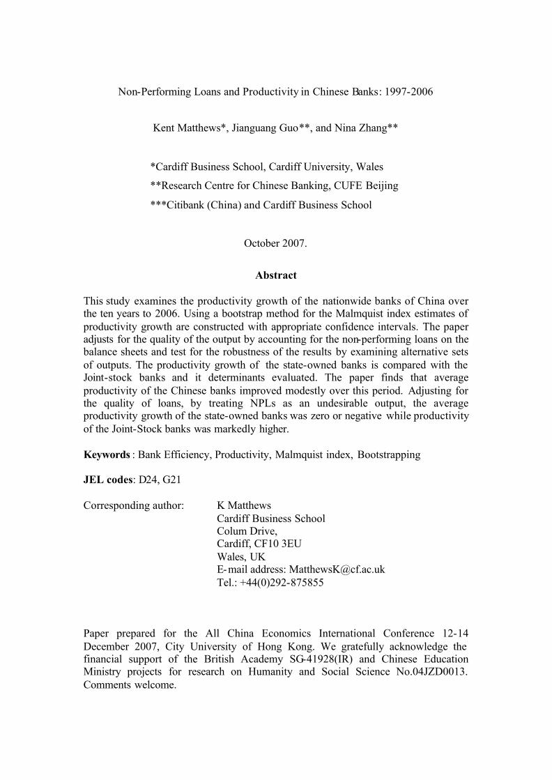
Table 4 b: Productivity Measures, Model 2, Standard error bounds in parenthesis Bank



1.0036* (0.8485, 0.9465)

0.9486 (0.8897, 1.0510)

1.0579* (0.8601, 0.9919)

Bank of China

1.0280 (0.9646, 1.3188)

1.0000 (0.6089, 1.0397)

1.0280* (1.1270, 1.6736)


1.0431 (0.9046, 1.0864)

1.0602 (1.0069, 1.2527)

0.9839* (0.7978, 0.9675)

Industrial and Comm Bank China

1.1170* (0.8838, 1.0331)

1.0020 (0.8156, 1.0058)

1.1148 (0.9634, 1.1446)


0.9259 (0.6883, 0.9761)

1.0423* (0.4715, 0.8599)

0.8883* (1.0231, 1.5074)


0.6281* (1.3119, 2.0213)

1.0000 (0.5361, 1.1254)

0.4894* (1.3931, 2.7048)

China Merchant Bank

0.7499* (1.0295, 1.4790)

1.0000 (0.5783, 1.1059)

0.7499* (1.1757, 1.8527)


0.5942* (0.7556, 1.1320)

1.0000 (0.5105, 1.0343)

0.5942* (0.9303, 1.5676)

China Minsheng Bank

0.6499* (0.9083, 1.3805)

1.0000 (0.6441, 1.2821)

0.64992* (0.9751, 1.4536)


1.2107 (1.0093, 1.8375)

1.0000* (0.2596, 0.8031)

1.2107* (2.0305, 3.4981)

Hua Xia Bank

0.7093* (0.9560, 1.4560)

1.0466 (0.6129, 1.2131)

0.6777* (1.0582, 1.6218)


0.7150* (0.7507,1.0617)

0.9809 (0.9279, 1.5380)

0.7290 (0.6284, 0.8519)


0.7846* (0.8366, 1.1353)

0.9739 (0.7654, 1.2902)

0.8056 (0.7992, 1.374)

16

Table 4 c: Productivity Measures, Model 3, Standard error bounds in parenthesis. Bank



0.3847* (0.3874, 0.6276)

0.5236 (0.3389, 0.6070)

0.7347* (0.7928, 1.3809)

Bank of China

1.0627* (1.3868, 1.8048)

1.5543* (0.7126, 1.4605)

0.6833* (0.9209, 2.1134)


0.2264 (0.1952, 0.3440)

0.3172 (0.1691, 0.3548)

0.7136* (0.7498, 1.3435)


0.6195* (0.7269, 1.1843)

0.9258 (0.5826, 1.0977)

0.6691* (0.8202, 1.4910)


1.0276* (1.9608, 3.1976)

1.7090* (0.8470, 1.6662)

0.6013* (1.4537, 2.7264)


0.5449* (1.8324, 2.7091)

1.0000 (0.5347, 1.1527)

0.5449* (1.7883, 3.8510)

China Merchant Bank

0.5746* (0.8876, 1.5353)

1.0000* (0.4406, 0.9721)

0.5746* (1.1544, 2.3589)


1.7830* (0.8117, 1.5887)

1.0000* (0.0225, 0.2021)

1.7830* (6.1013, 16.9400)

China Minsheng Bank

0.3847* (1.2096, 1.9079)

0.8131 (0.4365, 0.9262)

0.4731* (1.5395, 3.1522)


0.4974* (0.8627, 1.5605)

1.0000 (0.5769, 1.5683)

0.4974* (0.7606, 1.571)

Hua Xia Bank

0.4087* (1.759, 2.7824)

0.9979 (0.5516, 1.1367)

0.4096* (1.8503, 3.6536)


0.2194* (0.4682, 0.8424)

0.4128 (0.2041, 0.5287)

0.5314* (1.2121, 2.4761)


0.4253* (0.5894, 1.0280)

0.6073 (0.3294, 0.7123)

0.6345* (1.0925, 2.0750)

17

Table 4 d: Productivity Measures, Model 4, Standard error bounds in parenthesis. Bank



0.4974* (0.7083, 0.9396)

0.4461 (0.3099, 0.4644)

1.1151* (1.754, 2.5327)

Bank of China

1.0280* (1.1311, 1.8204)

1.0000 (0.6098, 1.0099)

1.0280* (1.5509, 2.3578)


0.5242* (0.6633, 0.9885)

0.4251 (0.2239, 0.4551)

1.2332* (1.8189, 3.1432)


0.5205* (0.5934, 0.8620)

0.3920* (0.1800, 0.3875)

1.32377* (1.8985, 3.3426)


0.9442* (1.0735, 1.6368)

0.9672* (0.4055, 0.8915)

0.9762* (1.4834, 2.7995)


0.8718* (2.1857, 4.4171)

1.0004 (0.5667, 1.1919)

0.8715* (2.2100, 5.4806)

China Merchant Bank

0.7762* (1.5344, 2.3761)

1.0000 (0.5933, 1.1702)

0.7762* (1.5909, 2.8590)


2.4432 (1.8925, 4.1542)

1.0000* (-0.0561, 0.4120)

2.4432 (2.0436, 41.644)

China Minsheng Bank

0.8922* (1.7427, 3.6739)

1.0000 (0.7186, 1.4233)

0.8922* (1.6044, 3.5296)


1.2846* (1.6997, 3.4786)

1.0000* (0.2804, 0.7386)

1.2846* (3.7000, 6.6736)

Hua Xia Bank

0.8463* (1.9575, 3.4540)

1.0547 (0.6823, 1.3436)

0.8024* (1.7472, 3.7025)


0.7492* (1.0595, 2.1492)

0.5636 (0.2986, 0.6328)

1.3294* (2.0061, 5.0530)


0.6581* (0.9730, 1.4484)

0.6687 (0.3897, 0.7972)

0.9841* (1.4231, 2.7491)

Mean estimates were obtained from 1000 bootstrap generations for each pair

of years for the 14 banks for the period 1997-2003 and 13 banks for 2004-2006. To

make the presentation easier, the 14 banks were sub-divided into the big-4 SOBs, the

next largest five banks and the bottom five banks. Tables 5 a – c report the weighted

(by asset share) mean values of the bias adjusted bootstrap estimates of the models for

the Malmquist productivity index, increase in efficiency (catch-up) and technical

18

progress with indicators of statistical significance. An indicator of significance states

that the bias-corrected estimate is significantly different from unity (no change).

Table 5a - Weighted Mean Changes in Productivity (Malmquist) Model Year SOB-4 Top-5 JSB Lower-5 JSB

1998/97 1.0474*** 1.3861*** 2.2090*** 1999/98 0.9692 1.2426 1.0510 2000/99 0.9058*** 0.9819*** 0.7940*** 2001/00 0.8987*** 0.9044*** 0.7840*** 2002/01 0.9721*** 1.0741** 0.9207*** 2003/02 0.9500*** 0.9787 0.8456*** 2004/03 1.0642*** 1.0182 1.3756** 2005/04 1.1154*** 1.1085*** 0.8609*** 2006/05 0.8760*** 1.0267 0.9082*** 1997/06 0.9409 1.8350*** 1.0949

Model 1 Loans Unadjusted 2 inputs 4 outputs

1998/97 1.0202** 1.1099*** 1.1557*** 1999/98 0.9841 1.0370 1.0490** 2000/99 1.0235 0.9912 1.0032 2001/00 1.0541** 0.8929*** 0.9244*** 2002/01 1.0086 1.1093*** 1.0451* 2003/02 0.9721*** 0.9543*** 0.9375*** 2004/03 0.9963 1.0349 1.2462 2005/04 0.9854 0.9658 0.9593 2006/05 1.0457*** 1.0029 0.9393*** 1997/06 0.9912 1.0240 1.1471

Model 2 Loans Unadjusted 3 inputs 3 outputs

1998/97 1.0100*** 1.5740*** 2.1236*** 1999/98 0.9720 1.2321*** 1.1266*** 2000/99 0.9968 1.0392 0.9340 2001/00 0.9642* 0.8812*** 0.7990*** 2002/01 0.9793** 1.0601* 0.9093*** 2003/02 0.8831*** 0.9373*** 0.8687*** 2004/03 0.9795*** 0.9385** 1.0715*** 2005/04 1.0511*** 1.0657*** 0.8861*** 2006/05 0.8767*** 1.0450 0.9231**

Model 3 Loans adjusted 2 inputs 4 outputs

1997/06 0.8417** 1.9463*** 1.2565**

1998/97 1.0391*** 1.3754*** 1.1822*** 1999/98 0.8773*** 1.0900** 1.1222*** 2000/99 1.1032*** 1.0970*** 1.2217*** 2001/00 0.9939 0.9010*** 0.9312*** 2002/01 0.9744*** 1.1029*** 1.2080*** 2003/02 0.9518*** 1.0137 0.9672 2004/03 0.9875 0.9834 1.0341

Model 4 Loans adjusted 3 inputs 3 outputs

2005/04 0.9715*** 0.9738 0.9351

19

2006/05 1.0685*** 1.0194 0.9416*** 1997/06 0.9510 2.1974*** 2.0477***

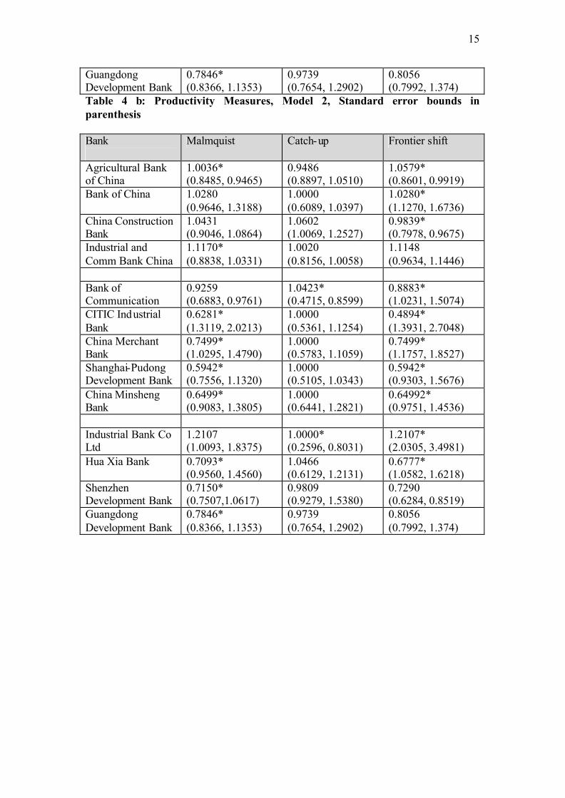
*** significant at the 1%, ** significant at the 5%, * significant at the 10% Table 5b - Weighted Mean Changes in Efficiency (Catch-up) Model Year SOB Top 5 JSB Lower 5 JSB

1998/97 0.9124 1.0034 1.4908* 1999/98 0.9452 1.1260 1.2334 2000/99 1.0980 0.8731 0.6195*** 2001/00 0.8275*** 0.9687 0.8937 2002/01 0.8654*** 1.0479 1.0795 2003/02 0.9903 1.1818** 0.9505 2004/03 0.9857 0.9661 0.8777 2005/04 1.3681*** 1.3681 0.9143 2006/05 0.9840 0.9998 0.8815*

Model 1

1997/06 0.9033 0.9271 0.7994*

1998/97 1.0405 0.9381 0.9043 1999/98 1.1994*** 1.1455* 1.1022 2000/99 1.0488 0.9010 0.8745** 2001/00 1.0125 0.9869 0.9987 2002/01 0.8162*** 1.0159 1.0708 2003/02 0.9309*** 0.9433 0.9197 2004/03 0.9182** 0.9492 0.7849*** 2005/04 0.9648 0.9759 1.1429** 2006/05 1.0176 0.9866 0.9463

Model 2

1997/06 0.9527 0.7797*** 0.9015

1998/97 0.8843 1.0907 1.5923** 1999/98 0.6997*** 0.9417 0.8562 2000/99 1.1559 0.9098 0.7959*** 2001/00 0.8287*** 0.9444 0.9223 2002/01 0.8870** 1.0569 1.0153 2003/02 1.0111 1.1687*** 0.9818 2004/03 0.9930 0.9019 1.1145 2005/04 1.4162*** 1.0081 0.9886 2006/05 0.9859 1.0115 0.8873

Model 3

1997/06 0.6838*** 0.8446 0.7248**

1998/97 0.7628*** 0.9536 0.8164* 1999/98 0.9692 1.0873 1.0199 2000/99 0.9187 0.8688* 0.9381 2001/00 0.9613 1.0122 1.0216 2002/01 0.7993*** 1.0862 1.2010*** 2003/02 0.9162*** 0.9287 0.8144*** 2004/03 0.9973 0.9070 1.0098

Model 4

2005/04 0.9479** 0.9685 1.1590**

20

2006/05 1.0294 0.9966 0.9228 1997/06 0.4329*** 0.7152*** 0.6496***

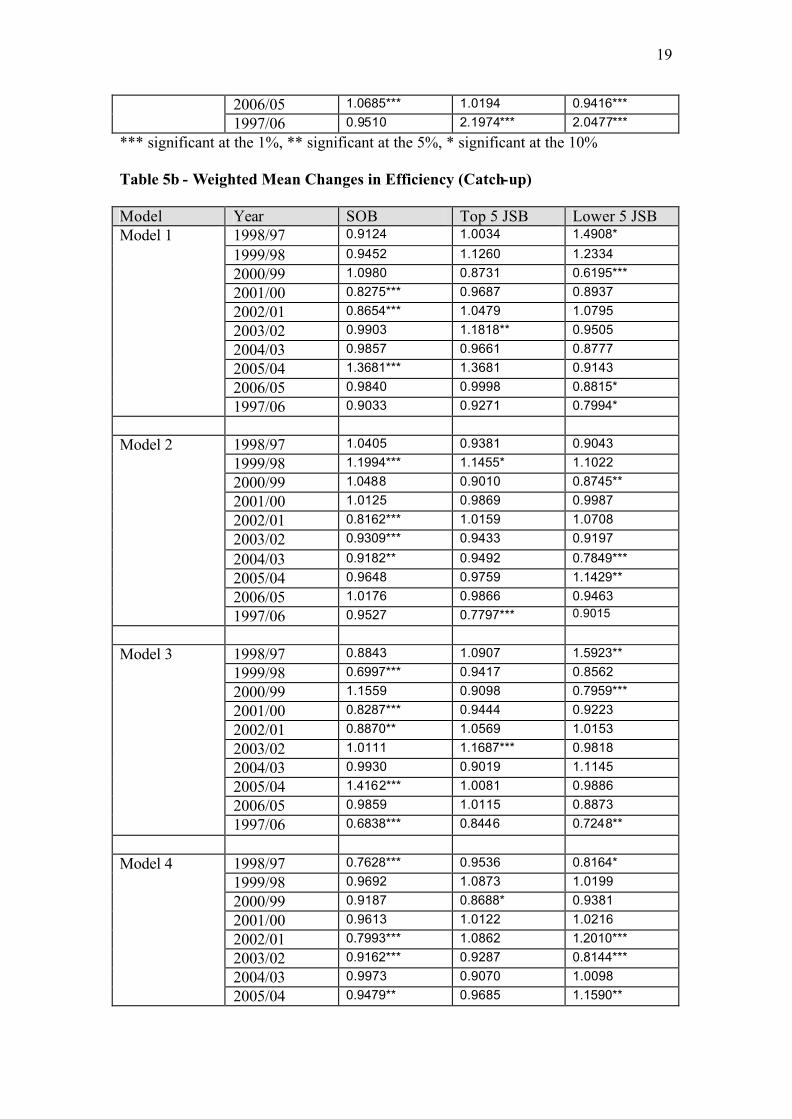
*** significant at the 1%, ** significant at the 5%, * significant at the 10% Table 5c - Weighted Mean Changes in Technology (Technical progress) Model Year SOB Top 5 JSB Lower 5 JSB

1998/97 1.1726 1.4022** 1.4497** 1999/98 1.0421 1.1467 0.8831 2000/99 0.8708* 1.1677 1.3617** 2001/00 1.0886 0.9553 0.8864 2002/01 1.1364* 1.0920 0.8863 2003/02 0.9720 0.8478 0.8940 2004/03 1.0852 1.0802 3.1427*** 2005/04 0.8203*** 1.1873 0.9609 2006/05 0.8996 1.0505 1.0376

Model 1

1997/06 1.0271 2.0031*** 1.4296**

1998/97 0.9844 1.1927*** 1.4968*** 1999/98 0.8301*** 0.9274 0.9632 2000/99 0.9949 1.1197 1.1812*** 2001/00 1.0488 0.9106* 0.9324 2002/01 1.2783*** 1.1936*** 0.9829 2003/02 1.0470* 1.0169 1.0224 2004/03 1.12812** 1.1264 4.0554*** 2005/04 1.0250 1.0114 0.8581*** 2006/05 1.0267 1.0295 1.0020

Model 2

1997/06 1.0618 1.3290*** 1.5166***

1998/97 1.1748 2.6606*** 1.3130* 1999/98 1.4604*** 1.3542*** 1.3452** 2000/99 0.9022 1.1531 1.1975* 2001/00 1.1664** 0.9460 0.8696* 2002/01 1.1312* 1.1268 0.9308 2003/02 0.8836*** 0.8254*** 0.8896 2004/03 0.9907 1.0559 0.9773 2005/04 0.7441*** 1.0741 0.9055 2006/05 0.8990 1.0573 1.0505

Model 3

1997/06 1.1938 3.5628*** 1.8122**

1998/97 1.5591*** 2.5068*** 1.76969*** 1999/98 0.9169 1.0391 1.1148 2000/99 1.2116*** 1.2832*** 1.34073*** 2001/00 1.0391 0.9014* 0.9205 2002/01 1.2802*** 1.1168 1.0084 2003/02 1.0438 1.1029* 1.1886*** 2004/03 1.0006 1.0955 1.0388

Model 4

2005/04 1.0289 1.0253 0.8307***

21

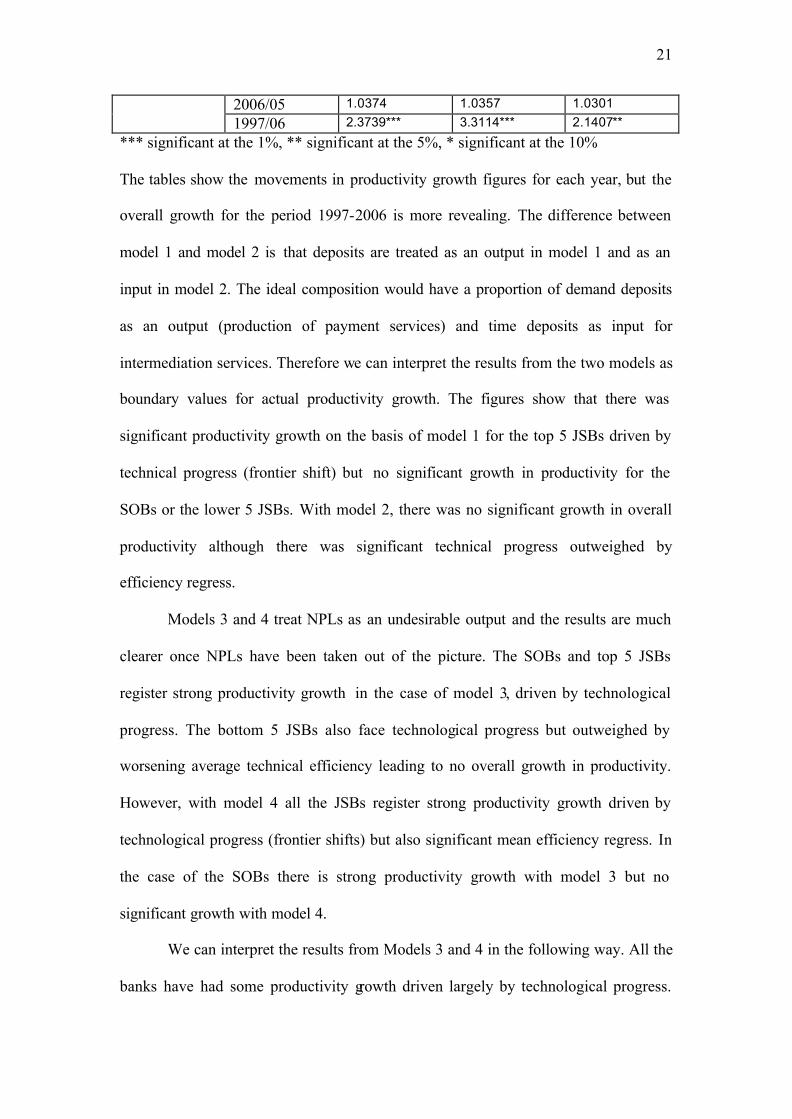
2006/05 1.0374 1.0357 1.0301 1997/06 2.3739*** 3.3114*** 2.1407**

*** significant at the 1%, ** significant at the 5%, * significant at the 10% The tables show the movements in productivity growth figures for each year, but the

overall growth for the period 1997-2006 is more revealing. The difference between

model 1 and model 2 is that deposits are treated as an output in model 1 and as an

input in model 2. The ideal composition would have a proportion of demand deposits

as an output (production of payment services) and time deposits as input for

intermediation services. Therefore we can interpret the results from the two models as

boundary values for actual productivity growth. The figures show that there was

significant productivity growth on the basis of model 1 for the top 5 JSBs driven by

technical progress (frontier shift) but no significant growth in productivity for the

SOBs or the lower 5 JSBs. With model 2, there was no significant growth in overall

productivity although there was significant technical progress outweighed by

efficiency regress.

Models 3 and 4 treat NPLs as an undesirable output and the results are much

clearer once NPLs have been taken out of the picture. The SOBs and top 5 JSBs

register strong productivity growth in the case of model 3, driven by technological

progress. The bottom 5 JSBs also face technological progress but outweighed by

worsening average technical efficiency leading to no overall growth in productivity.

However, with model 4 all the JSBs register strong productivity growth driven by

technological progress (frontier shifts) but also significant mean efficiency regress. In

the case of the SOBs there is strong productivity growth with model 3 but no

significant growth with model 4.

We can interpret the results from Models 3 and 4 in the following way. All the

banks have had some productivity growth driven largely by technological progress.

22

However, this has favoured the benchmarks banks that have improved productivity

faster than the rest leading to average efficiency regress. Figure 2 below summarises

the performance of the three groups of banks according to the type of model against

the null hypothesis of zero productivity growth (Malmquist index M = 1)

Figure 2

The bold line indicates the null of zero overall productivity growth (M = 1) for

the full time period 1997-2006 under the assumption of each model. The SOBs show

no significant productivity growth and show a significant productivity regress on the

assumption of model 3, where NPLs are treated as a negative output and deposits are

treated as an output. The top 5 JSBs show significant productivity growth in the case

of model 1, model 3 and model 4 while the lower 4 JSBs show significant

productivity growth in case of model 3 and model 4. The adjustment for NPLs

indicates a marked difference in performance between the SOBs and the JSBs over

the full period. The figure shows graphically that the Top 5 JSBs dominate in terms of

overall performance followed by the remaining cluster of JSBs.

SOB

Top 5 - JSB

Other JSB

Model 1

Model 2

Model 3

Model 4

23

We now turn to an analysis of the characteristics of productivity growth by

examining its determinants. The raw material of what is to be explained on a yearly

basis is the bootstrap mean value of the Malmquist productivity index for each bank

under the assumption of each of the models 1-4. Table 6 shows some selected results

from panel corrected heteroskedastic adjustment10. The bank specific variables are;

LSIZE is the natural logarithm of total assets, COST is the cost- income ratio, SOB is a

dummy variable for state-owned banks, FOR is the foreign ownership stake given by

Table 2, FEE is the proportion of revenue from net fees and commissions, IPO is a

dummy variable for the year of the bank listing on the domestic stock exchange.

Table 6: Dependant variable: Malmquist productivity index. Panel heteroskedastic adjusted standard errors; No: of obs=123, No: of groups=14. Variable Model 1 Model 2 Model 3 Model 4

Intercept 3.51*** 2.38*** 1.83*** 1.71*** 3.49*** 2.45*** 2.07*** 1.99***

LSIZE -.19* -.11*** -.06*** -.06*** -.19* -.11** -.08*** .08***

COST -.003 - -.001 - -.001 - -.001 -

SOB .315 - .152** .133** .312 - .133 .128

FOR .017** .015*** .007*** .007*** .010 .008* .002 .002

FEE .018*** .019*** .002* .002*** .016*** .017*** .003* .003**

IPO -.129 -.152 .004 - -.146** -.176** -.020 -

R-sq 0.1505 0.1310 0.1185 0.1078 0.1757 0.1533 0.1362 .1316

*** significant at 1%, ** significant at 5%, * significant at 10%

The two consistent determinants for all four models is size, measured by total assets,

and the composition of revenue. The sign on the variable LSIZE suggests that the

larger the bank, the lower the growth in productivity. An indicator of managerial

10 The standard fixed effects model was rejected on conventional F test for each of the models.

24

flexibility and capability to diversify output is given by the composition of earnings

from off-balance sheet sources. The sign on FEE suggests that the greater the

composition of fee income in revenue, the greater the productivity growth. There is

weak evidence that foreign financial institutional shareholding is associated with

higher productivity growth but this affect is weakened when NPLs are treated as an

undesirable output. There is no evidence that productivity growth is obtained through

cost reduction and there is little evidence that state-owned banks have a productivity

advantage. The extension of ownership from state and local government to the

domestic public through listing on the domestic exchanges has had mostly no

statistical effect on productivity. Where significant, this variable enters with a

negative sign.

6.0 Conclusion

This paper has used the Malmquist decomposition to quantify the productivity

growth of Chinese banks in 1997-2006. The advantage of use the Malmquist method

is that it separates the diffusion of technology (efficiency gains) from advances in

technology (frontier shifts). The paper also applies bootstrapping techniques to

evaluate significant changes in productivity, efficiency gains and innovation.

Using deposits as an output, only the top 5 JSBs showed significant

productivity gains driven by strong technological advances over this period. When

deposits are treated as an input, productivity growth is zero with technological gains

being offset by average efficiency regress.

Once NPLs are treated as an undesirable output the picture becomes clearer.

At best there is on average no productivity growth for the SOBs and at worst, there is

average productivity regress. Technological gains have been swamped by average

25

efficiency losses. However, the JSBs show strong productivity growth driven by

spectacular innovation effects. While adopting technologies that improved the

productivity of the average JSB, the average JSB failed to keep up with the

benchmark banks and moved further away from the frontier.

An econometric analysis confirms that the larger banks had lower productivity

growth than smaller banks. This may be explained by the political and social

opposition the SOBs face in attempting to restructure factor inputs and downsize as a

means of improving performance. It also explains the concentration of the activity of

the Asset Management Companies on the SOBs in aiding the divestiture of their large

NPL holdings.

Higher productivity growth was also associated with banks that had diversified

into non- interest earnings activity. The higher the proportion of revenue from non-

interest earnings indicates greater management flexibility and an increase in the

productivity of the banks.

The analysis also revealed weak evidence that the stronger the foreign

financial institutional stake in the bank, the greater the productivity growth of the

bank. However, as Table 2 shows, this aspect is relatively recent in the sample frame

and until further data is available, requires a cautious assessment.

26

References

Alam I S (2001), ‘A Nonparametric Approach for Assessing Productivity Dynamics of Large US Banks’, Journal of Money, Credit and Banking, 33, 121-139 Barnett W, Offenbacher E and Spindt P (1984), ‘The New Divisia Monetary Aggregates’, Journal of Political Economy, 92, 1049-1085 Baumol, W (1982) ‘Contestable Markets: an Uprising in the Theory of Industry Structure’, American Economic Review 72, 1-15. Berg S, Finn R and Eilev S (1992), ‘Malmquist Indices of Productivity Growth during the deregulation of Norwegian Banking, 1980-89’, Scandinavian Journal of Economics, 94, (supplement) 211 – 228 Casu B, Girardone C and Molyneux P (2004), ‘Productivity change in European banking: A comparison of parametric and non-parametric approaches’, Journal of Banking and Finance, 28, 2521-2540 Chen X, Skully M and Brown K (2005), "Banking Efficiency in China: Applications of DEA to pre-and post-Deregulation eras: 1993-2000", China Economic Review, 16, 2229-245 Färe R, Grosskop S and Norris M (1994), Productivity Growth, Technical Progress, and Efficiency Change in Industrialized Countries’, American Economic Review, 84, 66-83 Fu X and Heffernan S (2005), "Cost X-efficiency in China's Banking Sector", Cass Faculty of Finance Working Paper #WP-FF-14-2005 Fukuyama, H. (1995). “Measuring efficiency and productivity growth in Japanese banking: A non-parametric frontier approach”, Applied Financial Economics, 5, pp. 95-117. Goldscmidt A (1981), ‘On the definition and measurement of bank output’, Journal of Banking and Finance, 5, 575-581 Grifell-Tatjé E and Lovell C (1997), ‘The sources of productivity change in Spanish banking’, European Journal of Operational Research, 98, 364-380 Grosskopf, S (2003). “Some remarks on Productivity and its decompositions”, Journal of Productivity Analysis 20, pp. 459-474. Isik I and Hassan (2003), ‘Financial deregulation and total factor productivity change: An empirical study of Turkish commercial banks’, Journal of Banking and Finance, 27, 1455-1485 La Porta R, Lopez-de-Silanese, Shleifer F, Vishny R (2002), "Government Ownership of Banks", Journal of Finance, 57, 265-302

27

Liu C and Song W (2004), "Efficiency Analysis in China Commercial Banks based on SFA", Journal of Financial Research, 6, 138-142 Lothgreen M and Tambour M (1999), ‘Bootstrapping the data envelope analysis Malmquist productivity index’, Applied Economics, 31, 417-425 Lovell, C.A.K., (2003), ‘The decomposition of Malmquist productivity indexes’ Journal of Productivity Analysis, 20, 437-458. Matthews K, Guo J and Zhang X (2007a), ‘Rational Inefficiency and non-performing loans in Chinese banking: A non-parametric bootstrapping approach’, China Finance Review, 1, 3, 55-75 Matthews K, Guo J and Zhang X (2007b), ‘X-efficiency versus Rent-Seeking in Chinese banks, 1997-2006’, paper presented to Australian Economics Association conference, Hobart, Tasmania, September 2007. Mukherjee K, Ray K, Miller S (2001), ‘Productivity growth in large US commercial banks: The initial post-deregulation experience’ Journal of Banking and Finance, 25, 913-939 Neal P (2004), ‘Efficiency and Productivity Change in Australian Banking’, Australian Economic Papers, 43, 174-192 Noulas A (1997), ‘Productivity Growth in the Hellenic Banking Industry: State versus Private Banks, Applied Financial Economics, 7, 223-228 Park K and Weber W (2006), ‘A Note on efficiency and productivity growth in the Korean Banking Industry, 1992 – 2002’, Journal of Banking and Finance, 30, 2371-2386 Qian Q (2003), "On the Efficiency Analysis of SFA in China Commercial Banks", Social Science of Nanjing, 1, 41-46 (Chinese language) Ray, S.C. and Desli, E. (1997). “Productivity growth, technical progress and efficiency change in industrialised countries: Comment”, The American Economic Review 87, 1033-1039. Simar L and Wilson P (1999), ‘Estimating and bootstrapping Malmquist indices’, European Journal of Operational Research, 11, 459-471 Sun Z (2005), "Frontier Efficiency Analysis for the State-Owned Banks in China, Industrial Economics Research, 3, 41-47 (Chinese language) Tortosa-Ausina E, Grifell-Taté E, Armero C and Conesa D (2008), ‘Sensitivity analysis of Efficiency and Malmquist productivity indices: An application to Spanish Savings banks’, forthcoming, European Journal of Operational Research, 184, 1062-1084

28

Murillo-Melchor C, Pastor J M and Tortosa-Ausin E (2005), ‘Productivity growth in European banking’, Universtat Jaume I, Department d’Economia, Working Paper Qing W and Ou Y (2001), "Chinese Commercial Banks: Market Structure, Efficiency and its Performance" Economic Science, 100871, 34-45 (Chinese language) Wei Y and Wang L (2000), "The Non-Parametric Approach to the Measurement of Efficiency: The Case of China Commercial Banks", Journal of Financial Research, 3, 88-96 (Chinese language) Wheelock, D.C. and Wilson, P.W. (1999), “Technical progress, inefficiency and productivity change in U.S. banking, 1984-1993”, Journal of Money, Credit and Banking 31, 212-234. Worthington A (1999), ‘Malmquist Indices of Productivity Change in Australian Financial Services’, Journal of International Financial Markets and Money, 9 303-320 Xu Z, Junmin Z and Zhenseng J (2001), "An Analysis of the Efficiency of State-Owed Banks with Examples", South China Financial Research, 16, 1, 25-27 (Chinese language) Xue F and Yang D (1998), "Evaluating Bank Management and Efficiency using the DEA Model", Econometrics and Technological Economy Research, 6, 63-66 (Chinese language) Zhang C, Gu F and Di Q (2005), "Cost Efficiency Measurement in China Commercial Banks based on Stochastic Frontier Analysis", Explorations in Economic Issues, 6, 116-119 (Chinese language) Zhao X (2000), "State-Owned Commercial Banks Efficiency Analysis", Journal of Economic Science", 6, 45-50 (Chinese language)

cardiff business school working paper series · 2017-02-07 · cardiff business school colum drive,...

Documents