career concerns with exponential learningbonatti/concerns.pdfjel classification. d82, d83, m52. 1....

Theoretical Economics 12 (2017), 425–475 1555-7561/20170425

Career concerns with exponential learning

Alessandro BonattiSloan School of Management, MIT

Johannes HörnerDepartment of Economics, Yale University

This paper examines the interplay between career concerns and market structure.Ability and effort are complements: effort increases the probability that a skilledagent achieves a one-time breakthrough. Wages are based on assessed ability andon expected output. Effort levels at different times are strategic substitutes and,as a result, the unique equilibrium effort and wage paths are single-peaked withseniority. Moreover, for any wage profile, the agent works too little, too late. Com-mitment to wages by competing firms mitigates these inefficiencies. In that case,the optimal contract features piecewise constant wages and severance pay.

Keywords. Career concerns, experimentation, career paths, up-or-out, reputa-tion.

JEL classification. D82, D83, M52.

1. Introduction

Career concerns are an important driver of incentives. This is particularly so inprofessional-service firms, such as law and consulting, but applies more broadly to en-vironments in which creativity and originality are essential for success, including phar-maceutical companies, biotechnology research labs, and academia. Market structurediffers across those industries, and so do labor market arrangements. Our goal is to un-derstand how market structure (in particular, firms’ commitment power) affects careerconcerns, and the resulting patterns of wages and performance. As we show, commit-ment leads to backloading of wages and effort, relative to what happens under spotcontracting.

Alessandro Bonatti: [email protected] Hörner: [email protected] paper previously circulated under the title “Career concerns and market structure.” Bonatti acknowl-edges the support of MIT’s Program on Innovation in Markets and Organizations (PIMO). Hörner gratefullyacknowledges support from NSF Grant SES 092098. We would like to thank Daron Acemoglu, Glenn Ellison,Bob Gibbons, Michael Grubb, Hugo Hopenhayn, Tracy Lewis, Nicola Persico, Scott Stern, Steve Tadelis, Ju-uso Toikka, Jean Tirole, Alex Wolitzky, and, especially, Joel Sobel, as well as participants at ESSET 2010, the2011 Columbia–Duke–Northwestern IO Theory Conference, and audiences at the Barcelona JOCS, Berke-ley, Bocconi, CIDE, Collegio Carlo Alberto, EUI, LBS, LSE, MIT, Montreal, Northwestern, Nottingham, NYU,Penn State, Stanford, Toronto, UBC, USC, IHS Vienna, and Yale for helpful discussions, and Yingni Guo forexcellent research assistance.

Copyright © 2017 The Authors. Theoretical Economics. The Econometric Society. Licensed under theCreative Commons Attribution-NonCommercial License 3.0. Available at http://econtheory.org.DOI: 10.3982/TE2115

http://econtheory.org/

mailto:[email protected]

mailto:[email protected]

http://creativecommons.org/licenses/by-nc/3.0/

http://econtheory.org/

http://dx.doi.org/10.3982/TE2115

426 Bonatti and Hörner Theoretical Economics 12 (2017)

Our point of departure from nearly all the existing literature on career concerns,starting with Holmström (1982/1999), involves the news process. The ubiquitous as-sumption that rich measures of output are available throughout is at odds with the struc-ture of learning in several industries. To capture the features of research-intensive andcreative industries, we assume that success is rare and informative about the worker’sskill. Breakthroughs are defining moments in a professional’s career. In other words,information is coarse: either an agent reveals himself to be talented through a (first)breakthrough or he does not. Indeed, in many industries, there is growing evidence thatthe market rewards “star” professionals.1

Our assumption on the contracting environment follows the literature on careerconcerns. Explicit output-contingent contracts are not used. While theoretically attrac-tive, innovation bonuses in research and development (R&D) firms are hard to imple-ment due to complex attribution and timing problems. Junior associates in law andconsulting firms receive fixed stipends. In the motion pictures industry, most contractsinvolve fixed payments rather than profit-sharing (see Chisholm 1997).2

In our model, information about ability is symmetric at the start.3 Skill and out-put are binary, and effort is continuous. Furthermore, skill and effort are complements:only a skilled agent can achieve a high output, or breakthrough. The breakthrough timefollows an exponential distribution, whose intensity increases with the worker’s unob-served effort. Hence, effort increases not only expected output, but also the rate of learn-ing, unlike in the additive Gaussian setup. When a breakthrough obtains, the marketrecognizes the agent’s talent and that is reflected in future earnings. The focus is on therelationship until a breakthrough occurs.4 Throughout, the market is competitive. Wecontrast the equilibrium when firms can commit to long-term wage policies and whenthey cannot.

1Prominent examples include working a breakthrough case in law or consulting, signing a record deal,or acting in a blockbuster movie. See Gittelman and Kogut (2003) and Zucker and Darby (1996) for evidenceon the impact of “star scientists,” and Caves (2003) for a discussion of A-list vs. B-list actors and writers. Fora different example, consider a local politician who seeks to establish a reputation for “getting things done”by securing congressional funding for a major public good.

2It is not our purpose to explain why explicit contracts are not used. As an example that satisfies bothfeatures, consider the biotechnology and pharmaceutical industries. Uncertainty and delay shroud prof-itability. Scientific breakthroughs are recognized quickly, commercial ones not so. Ethiraj and Zhao (2012)find a success rate of 1�7% for molecules developed in 1990. The annual report by the Pharmaceutical Re-search and Manufacturers of America (PhRMA) (2012) shows even higher attrition rates. Because the Foodand Drug Administration (FDA) drug approval and molecule patenting are only delayed and noisy metricsof a drug’s profitability, they are rarely tied explicitly to a scientist’s compensation (see Cockburn et al. 2004).Likewise, few biotechnology companies offer variable pay in the form of stock options (see Stern 2004).

3One could also examine the consequences of overoptimism by the agent. In many applications, how-ever, symmetrical ignorance appears to be the more plausible assumption. See Caves (2003).

4In Section 4.1, we turn to the optimal design of an up-or-out arrangement, i.e., a deadline. A proba-tionary period is a hallmark of many occupations (law, accounting, and consulting firms, etc.). Thoughalternative theories have been put forth (e.g., tournament models), agency theory provides an appealingframework (see Fama 1980 or Fama and Jensen 1983). Gilson and Mnookin (1989) offer a vivid accountof associate career patterns in law firms, and the relevance of the career concerns model as a possibleexplanation.

Theoretical Economics 12 (2017) Career concerns with exponential learning 427

Spot contracts

Under spot contracts, the agent is paid his full expected marginal product at each mo-ment in time. Therefore, the agent’s compensation depends on the market’s expectationabout his talent and effort. In turn, this determines the value of incremental reputation,and hence his incentives to exert effort so as to establish himself as high skilled.5 Inequilibrium, both the agent’s effort level and wage are single-peaked functions of time.

A key driver of the equilibrium properties is the strategic substitutability effect be-tween incentives at different stages in a worker’s career. Suppose the market expectsthe agent to exert high effort at some point. Failure to generate a success would leadthe market to revise its belief downward and lower future wages. This provides strongincentives for effort. However, competitive wages at that time must reflect the resultingincreased productivity. In turn, this depresses the agent’s incentives and compensa-tion at earlier stages, as future wages make staying on the current job relatively moreattractive.

Strategic substitutability does not arise in Holmström’s additively separable modelor in the two-period model of Dewatripont et al. (1999a, 1999b), because career con-cerns disappear in the last period. Instead, the strategic complementarity between ex-pected and realized effort in the first period generates equilibrium multiplicity.

Despite the complementarity between skill and effort, equilibrium is unique in ourmodel, yielding robust yet sharp welfare predictions. In particular, effort underprovisionand delay obtain very generally. Because output-contingent payments are impossible,competition among employers calls for positive flow wages even after prolonged failure.As a result, career concerns provide insufficient incentives for effort independently fromany particular equilibrium notion. For any wage path, the total amount of effort exertedis inefficiently low. In addition, effort is exerted too late: a social planner constrained tothe same total amount of effort exerts it sooner.6 As we shall see, these properties alsohold under competition with long-term contracts.

The most striking prediction of our model in terms of observable variables—single-peaked real wages—cannot be explained by the existing models (Holmström, and De-watripont, Jewitt, and Tirole). Because successful agents are immediately promoted,single-peaked wages refer to wages conditional on prolonged failure. This prediction isborne out by the data in the two papers by Baker et al. (1994a, 1994b), arguably the mostwidely used data set on internal wage policy in the organizational economics literature.7

5This is in contrast with Holmström, where the marginal benefit from effort is history-independent. Thisimplies that reputation incentives evolve deterministically, decreasing over time as learning occurs, whilewages decrease stochastically.

6Characterizing the agent’s best reply to exogenous wages has implications for the agent’s behavior fol-lowing one of his own deviations. In particular, it helps clarify the effect of the agent’s private beliefs.

7Baker et al. (1994a) describe the data as containing “personnel records for all management employees ofa medium-sized U.S. firm in a service industry over the years 1969–1988.” While the data set is confidential(and hence we cannot relate the properties of the industry to the parameters of our model), the populationof employees is restricted to “exempt” management positions, i.e., those for whom career concerns aremost salient.


Their data show that both the dynamics of real wages and the timing of promotionsare heterogeneous across agents. Overall, Baker et al. (1994b) suggest that such hetero-geneity is indicative of a “common underlying factor, such as ability, driving both wageincreases and promotions.” At the aggregate level, yearly real wages decrease on aver-age, conditional on no promotion. However, this is not true at all tenure levels.8 Bakeret al. (1994b) provide more detail about the wage and promotion patterns of employeesin the lowest two levels of the firm’s hierarchy. Arguably, these are the employees withthe strongest potential for establishing a reputation.

Baker et al. (1994b) show that the pattern of real wages is inverse-U-shaped for em-ployees who are not promoted to the next level within 8 years. In other words, wagesincrease at first for all employees and then decline until the employee is promoted tothe next level in the firm’s hierarchy (if ever). In Section 3.4, we compare this pattern toour equilibrium wages.

There are, of course, alternative explanations: a combination of symmetric learningand accumulation of general human capital would suggest that, for a particular choiceof technology, a worker’s expected productivity may increase at first only to quickly de-cline in the absence of sufficiently positive signals. Yet our model matches the out-comes described in the data quite well, relying only on hidden talent and a lumpy outputprocess.

Long-term contracts

The flexibility of our model allows us to study reputation incentives under market struc-tures that are not tractable in the Gaussian framework. In particular, we consider long-term contracts. In many sectors, careers begin with a probationary period that leads toan up-or-out decision, and wages are markedly lower and more rigid before the tenuredecision than after. Specifically, we allow firms to commit to a wage path, but the agentmay leave at any time. To avoid “poaching,” the contract must perpetually deliver a con-tinuation payoff above what the agent can get on the market. This constraint impliesthat one must solve for the optimal contract in all possible continuation games, as theoffers of competing firms must themselves be immune to further poaching.

Long-term contracts can mitigate the adverse consequences of output-independentwages because the timing of payments affects the optimal timing of the agent’s effort.Because future wages paid in the event of persistent failure depress current incentives,it would be best to pay the worker his full marginal product ex ante. This payment beingsunk, it would be equivalent, in terms of incentives, to no future payments for failure atall. Therefore, if the worker can commit to a no-compete clause, a simple signing bonusis optimal.

In most labor markets workers cannot commit to such clauses. It follows that firmsdo not offer signing bonuses, anticipating the worker’s incentive to leave right after cash-ing them in. Lack of commitment on the worker’s side prevents payments coming beforethe corresponding marginal product obtains. Surprisingly, as far as current incentives

8See Table VI in Baker et al. (1994a).


are concerned, it is then best to pay him as late as possible. This follows from the value oflearning: much later payments discriminate better than imminent ones between skilledand unskilled workers. Because effort and skill are complements, a skilled worker islikely to succeed by the end. Hence, payments made in the case of persistent failure aretied more to the agent’s talent than to his effort. This mitigates the pernicious effect offuture wages on current incentives. Backloading payments also softens the no-poachingconstraint, as the worker has fewer reasons to quit.

To summarize, long-term contracts backload payments and frontload effort, relativeto spot contracts. Backloading pay and severance payments (as well as signing bonusesand no-compete clauses) are anecdotally common in industries with one-sided com-mitment, such as law or consulting. In other words, several regularities observed inpractice arise as optimal labor-market arrangements when firms compete with long-term contracts.

Related literature

The most closely related papers are Holmström (1982/1999), as mentioned, as well asDewatripont et al. (1999a, 1999b). In Holmström, skill and effort enter linearly and ad-ditively into the mean of the output that is drawn in every period according to a normaldistribution. Wages are as in our baseline model: the worker is paid upfront the expectedvalue of the output. Our model shares with the two-period model of Dewatripont, Jewitt,and Tirole some features that are absent from Holmström’s. In particular, effort and tal-ent are complements. We shall discuss the relationship between the three models atlength.

Our paper can also be viewed as combining career concerns and experimenta-tion. As such, it relates to Holmström’s original contribution in the same way as theexponential-bandits approach of Keller et al. (2005) does to the strategic experimenta-tion framework introduced by Bolton and Harris (1999).

As in Gibbons and Murphy (1992), our paper examines the interplay of implicitincentives (career concerns) and explicit incentives (termination penalty). It shareswith Prendergast and Stole (1996) the existence of a finite horizon, and thus, of com-plex dynamics related to seniority. See also Bar-Isaac (2003) for reputational incen-tives in a model in which survival depends on reputation. The continuous-time modelof Cisternas (2016) extends the Gaussian framework to nonlinear environments, butmaintains the additive separability of talent and action. Ferrer (2015) studies the ef-fect of lawyers’ career concerns on litigation in a model with complementarity betweeneffort and talent. Jovanovic (1979) and Murphy (1986) provide models of career con-cerns that are less closely related: the former abstracts from moral hazard and fo-cuses on turnover when agents’ types are match-specific; the latter studies executives’experience–earnings profiles in a model in which firms control the level of capital as-signed to them over time. Finally, Klein and Mylovanov (2016) analyze a career-concernsmodel of advice, and provide conditions under which reputational incentives over a longhorizon restore the efficiency of the equilibrium.

The binary setup is reminiscent of Mailath and Samuelson (2001), Bergemann andHege (2005), Board and Meyer-ter-Vehn (2013), and Atkeson et al. (2015). However, in


Bergemann and Hege (2005), the effort choice is binary and wages are not based onthe agent’s reputation, while Board and Meyer-ter-Vehn (2013) let a privately informedagent control the evolution of his type through his effort. In (the regulation model withreputation of) Atkeson et al. (2015), firms control their types through a one-time initialinvestment. Here instead, information is symmetric and types are fixed.9

Finally, several papers have already developed theories of wage rigidity and back-loading with long-term contracts, none based on career concerns (incentive provisionunder incomplete information), as far as we know. These are discussed in Section 5.

Structure

The paper is organized as follows: Section 2 describes the model; Section 3 analyzes thecase of spot contracts; Section 4 introduces probationary periods and discusses whathappens when the agent is impatient or when even a low-ability agent might succeedwith positive probability; Section 5 explores long-term contracts; Section 6 discussesthe case of observable effort; and Section 7 briefly describes other extensions.

2. The model

2.1 Setup

We consider the incentives of an agent (or worker) to exert hidden effort (or work). Timeis continuous, and the horizon (or deadline) is finite: t ∈ [0�T ], T > 0. Most results carryover to the case T = ∞, as shall be discussed.

There is a binary state of the world. If the state is ω = 0, the agent is bound to fail,no matter how much effort he exerts. If the state is ω = 1, a success (or breakthrough)arrives at a time that is exponentially distributed, with an intensity that increases in theinstantaneous level of effort exerted by the agent. The state can be interpreted as theagent’s ability, or skill. We will refer to the agent as a high- (resp., low-) ability agent if thestate is 1 (resp., 0). The prior probability of state ω= 1 is p0 ∈ (0�1).

Effort is a nonnegative measurable function of time. If a high-ability agent exerts ef-fort ut over the time interval [t� t+dt), the probability of a success over that time intervalis (λ+ut)dt. Formally, the instantaneous arrival rate of a breakthrough at time t is givenby ω · (λ + ut), with λ ≥ 0. Note that, unlike in Holmström’s model, but as in the modelof Dewatripont, Jewitt, and Tirole, work and talent are complements.

The parameter λ can be interpreted as the luck of a talented agent. Alternatively, itmeasures the minimum effort level that the principal can force upon the agent by directoversight, i.e., the degree of contractibility of the worker’s effort. Either interpretationmight require some adjustment: as minimum effort, it is then important to interpret theflow cost of effort as net of this baseline effort, and to be aware of circumstances in whichit would not be in either party’s interest to exert this minimum level.10 Fortunately, this

9Board and Meyer-ter-Vehn (2014) study the Markov-perfect equilibria of a game in which effort affectsthe evolution of the player’s type both under symmetric and asymmetric information.

10As a referee pointed out, too low an effort level may be undesirable from the agent’s point of view,whose effort “bliss point” need not be zero.


issue does not arise for the equilibrium analysis under either commitment assumption.As for the luck interpretation, it is then arguably extreme to assume that luck correlateswith ability, so that a low-ability agent is bound to fail. In Section 4.2 we provide a dis-cussion and numerical simulations of what happens when an agent of low ability is lesslikely to succeed for a given effort level, yet might do so nonetheless.

As long as a breakthrough has not occurred, the agent receives a flow wage wt . Fornow, think of this wage as an exogenous (integrable, nonnegative) function of time. Lateron, equilibrium constraints will be imposed on this function, and this wage will reflectthe market’s expectations of the agent’s effort and ability, given that the market values asuccess. The value of a success is normalized to 1.

In addition to receiving this wage, the agent incurs a cost of effort: exerting effortlevel ut over the time interval [t� t + dt) entails a flow cost c(ut)dt. We assume thatc is increasing, thrice differentiable, and convex, with c(0) = 0, limu→0 c

′(u) = 0 andlimu→∞ c′(u) = ∞.

After a breakthrough occurs, the agent is known to be of high ability, and can expecta flow outside wage of v > 0 until the end of the game at T . In line with the interpretationof wages throughout the paper, we think of this wage as the (equilibrium) marginal prod-uct of the agent in the activity in which he engages after a breakthrough. Thus the wagev is a (flow) opportunity cost that is incurred as long as no success has been achieved,which must be accounted for, not only in the worker’s objective function, but also in theobjective of the social planner.11 Note that this flow opportunity cost lasts only as longas the game does, so that its impact fades away as time runs out.

The outside option of the low-ability agent is normalized to 0. There is no discount-ing.12 We discuss the robustness of our results to the introduction of discounting inSection 4.2.

The worker’s problem can then be stated as follows: to choose u : [0�T ] → R+, mea-surable, to maximize his expected sum of rewards, net of the outside wage v,

Eu

[∫ T∧τ

0[wt − vχω=1 − c(ut)]dt

]�13

where Eu is the expectation conditional on the worker’s strategy u and τ is the time atwhich a success occurs (a random time that is exponentially distributed, with instanta-neous intensity at time t equal to 0 if the state is 0 and to λ+ut otherwise). The indicatorof event A is denoted by χA. Ignoring discounting is analytically convenient, but thereis no discontinuity.

Of course, at time t effort is only exerted and the wage wt collected, conditional onthe event that no success has been achieved. We shall omit saying so explicitly, as those

11In many applications, there is an inherent value in employing a “star,” a possible interpretation for v, assuggested by a referee. Another natural case is that in which v equals the flow value of success conditionalon ω = 1 and no effort by the agent. In Section 3.1, we establish that if successes worth 1 arrive at rateλ ≥ 0, then v = λ. In Section 3.2, we show that stronger results obtain for the case v = λ; other results can begeneralized, but not interior effort and equilibrium uniqueness.

12At the beginning of the Appendix, we explain how to derive the objective function from its discountedversion as discounting vanishes. Values and optimal policies converge pointwise.

13Stating the objective as a net payoff ensures that the program is well defined even when T = ∞.


histories are the only nontrivial ones. Given his past effort choices, the agent can com-pute his belief pt that he is of high ability by using Bayes’ rule. It is standard to showthat, in this continuous-time environment, Bayes’ rule reduces to the ordinary differen-tial equation

pt = −pt(1 −pt)(λ+ ut)� p0 = p0� (1)

Observing that

P[τ ≥ t] = P[ω = 0 ∩ τ ≥ t]P[ω = 0|τ ≥ t] = P[ω = 0]

P[ω = 0|τ ≥ t] = 1 −p0

1 −pt� (2)

the problem simplifies to the maximization of∫ T

0

1 −p0

1 −pt[wt − c(ut)− v]dt�14 (3)

given w, over all measurable u : [0�T ] →R+, subject to (1).Consider this last maximization. If the wage falls short of the outside option (i.e., if

wt − v is negative), the agent has an incentive to exert high effort to stop incurring thisflow deficit. Achieving this is more realistic when the belief p is high, so that this incen-tive should be strongest early on, when he is still sanguine about his talent. This suggestsan effort pattern that is a decreasing function of time, as in Holmström. However, thisignores that, in equilibrium, the wage reflects the agent’s expected effort. As a result, weshall show that this intuition is incorrect: equilibrium effort might be increasing, and ingeneral is a single-peaked function of time.

2.2 The social planner

Before solving the agent’s problem, we start by analyzing the simpler problem faced by asocial planner. Recall that the value of a realized breakthrough is normalized to 1. But abreakthrough only arrives with instantaneous probability pt(λ+ ut), as it occurs at rateλ + ut only if ω = 1. Furthermore, the planner internalizes the flow opportunity costv incurred by the agent as long as no breakthrough is realized. Therefore, the plannermaximizes ∫ T

0

1 −p0

1 −pt[pt(λ+ ut)− v− c(ut)]dt� (4)

over all measurable u : [0�T ] → R+, given (1). As for most of the optimization programsconsidered in this paper, we apply Pontryagin’s maximum principle to get a charac-terization. The proof of the next lemma and of all formal results can be found in theAppendix.

14We have replaced ptv by the simpler v in the bracketed term inside the integrand. This is because∫ T

0

pt

1 −ptvdt =

∫ T

0

v

1 −ptdt − vT�

and we can ignore the constant vT .


Lemma 1. The optimum exists. At any optimum, effort u is monotone in t. It is decreasingif and only if the deadline exceeds some finite length.

Because the belief p is decreasing over time, note that the marginal product is de-creasing whenever effort is decreasing, but the converse need not hold (as we will seein equilibrium). Monotonicity of effort can be roughly understood as follows. There aretwo reasons why effort can be valuable: because it helps reduce the time over which thewaiting cost v is incurred and because it helps avoid reaching the deadline without abreakthrough. The first effect encourages early effort, and the second effect encourageslater effort. When the deadline is short (and the final belief is high), terminal effort ishigh, and the efficient effort level is increasing throughout.

The effort level exerted at the deadline depends on how pessimistic the planner is atthat point. By standard arguments (see Appendix A.1), the social planner exerts an effortlevel that solves

pT = c′(uT )� (5)

This states that the expected marginal social gains from effort (i.e., success) should equalthe marginal cost. Note that the flow loss v no longer plays a role at that time.

2.3 Exogenous wages

We now consider the agent’s best response to an entirely exogenous wage path. Thisallows us to provide an analysis of reputation incentives that is not tied to any particularequilibrium notion. In addition, it will guide our analysis of off-path behavior.

Consider an arbitrary exogenous (integrable) wage path w : [0�T ] → R+. The agent’sproblem given by (3) differs from the social planner’s in two respects: the agent disre-gards the expected value of a success (in particular, at the deadline), which increaseswith effort, and he takes into account future wages, which are less likely to be pocketedif more effort is exerted. We start with a technical result stating there is a unique solu-tion (uniqueness is stated in terms of the state variable p, from which it follows that thecontrol u is also essentially unique, e.g., up to a zero measure set of times).

Lemma 2. There exists a unique trajectory p that solves the maximization problem (3).

What determines the instantaneous level of effort? Transversality implies that, at thedeadline, the agent exerts no effort:

c′(uT ) = 0�

Relative to the social planner’s trade-off in (5), the agent does not take into account thelump-sum value of success. Hence his effort level is nil for any pT .

It follows from Pontryagin’s theorem that the amount of effort exerted at time t solves

c′(ut) = max{−

∫ T

t(1 −pt)

ps

1 −ps[ws − c(us)− v]ds�0

}� (6)


The left-hand side is the instantaneous marginal cost of effort. The marginal benefit(right-hand side) can be understood as follows. Conditioning throughout on reachingtime t, the expected flow utility over some interval ds at time s ∈ (t�T ) is

P[τ ≥ s](ws − c(us)− v)ds�

From (2), recall that

P[τ ≥ s] = 1 −pt

1 −ps= (1 −pt)

(1 + ps

1 −ps

);

that is, effort at time t affects the probability that time s is reached only through thelikelihood ratio ps/(1 −ps). From (1), we obtain

ps

1 −ps= pt

1 −pte− ∫ s

t (λ+uτ)dτ�

and so a slight increase in ut decreases the likelihood ratio at time s precisely by−ps/(1 −ps). Combining, the marginal impact of ut on the expected flow utility at times is given by

−(1 −pt)ps

1 −ps[ws − c(us)− v]ds�

and integrating over s yields the result.Equation (6) establishes that increasing the wedge between the future rewards from

success and failure (v − ws) encourages high effort, ceteris paribus. Higher wages inthe future depress incentives to exert effort today, as they reduce this wedge. In par-ticular, when future wages are very high, the agent may prefer not to exert any effort,in which case the corner solution ut = 0 applies. That being said, throughout this sec-tion we restrict attention to wage functions wt for which the agent’s first-order conditionholds. In Section 3, we shall establish that the corner solution ut = 0 is never played inequilibrium.

The trade-off captured by (6) illustrates a key feature of career concerns in thismodel. Because information is coarse (either a success is observed or it is not), theagent can only affect the probability that the relationship terminates. It is then intuitivethat incentives for effort depend on future wage prospects (with and without a break-through).15 This is a key difference with Holmström’s model, where future wages adjustlinearly in output and incentives are therefore independent of the wage level itself. Inour model (see Section 3), the level of future compensation does affect incentives toexert effort in equilibrium.

In particular, higher wages throughout reduce the agent’s instantaneous effort levelpointwise, because the prospect of foregoing higher future wages depresses incentivesat all times. However, the relationship between the timing of wages and the agent’s op-timal effort is more subtle. In particular, as we shall see in Section 5, it is not true that

15Note also that, although learning is valuable, the value of information cannot be read off first-ordercondition (6) directly: the maximum principle is an “envelope theorem,” and as such does not explicitlyreflect how future behavior adjusts to current information.


pushing wages back, holding the total wage bill constant, necessarily depresses total ef-fort. As is clear from (6), higher wages far in the future have a smaller effect on current-period incentives for two reasons: the relationship is less likely to last until then and,conditional on reaching these times, the agent’s effort is less likely to be productive (asthe probability of a high type then is very low).

To understand how effort is allocated over time, let us differentiate (6). (See the proofof Proposition 1 for the formal argument.) We obtain

pt · c(ut+dt)︸︷︷︸cost saved

+ pt(v −wt)︸︷︷︸wage premium

+ c′′(ut)ut︸︷︷︸cost smoothing

= pt(λ+ ut)︸︷︷︸pr. of success at t

· c′(ut)� (7)

The right-hand side captures the gains from shifting an effort increment du from thetime interval [t� t+dt) to [t+dt� t+2 dt) (backloading ): the agent saves the marginal costof this increment c′(ut)du with instantaneous probability pt(λ + ut)dt, i.e., the proba-bility with which this additional effort will not have to be carried out. The left-hand sidemeasures the gains from exerting this increment early instead (frontloading ): the agentincreases by pt du the probability that the cost of tomorrow’s effort c(ut+dt)dt is saved.He also increases at that rate the probability of getting the “premium” (v −wt)dt aninstant earlier. Last, if effort increases at time t, frontloading improves the workload bal-ance, which is worth c′′(u)dudt. This yields the arbitrage equation (7) that is instructiveabout effort dynamics.16 The next proposition formalizes this discussion.

Proposition 1. If w is decreasing, u is a quasi-concave function of time; if w is nonde-creasing, u is strictly decreasing.

Hence, even when wages are monotone, the worker’s incentives need not be so. Notsurprisingly then, equilibrium wages, as determined in Section 3, will not be either.

2.4 Comparison with the social planner

The social planner’s arbitrage condition would coincide with the agent’s if there were nowages, although the social planner internalizes the value of possible success at futuretimes. This is because the corresponding term in (4) can be “integrated out,”∫ T

0

1 −p0

1 −ptpt(λ+ ut)dt = −(1 −p0)

∫ T

0

pt

(1 −pt)2 dt = (1 −p0) ln1 −pT

1 −p0�

so that it only affects the final belief, and hence the transversality condition. But theagent’s and the social planner’s transversality conditions do not coincide, even whenws = 0. As mentioned, the agent fails to take into account the value of a success at thelast instant. Hence, his incentives at T , and hence his strategy for the entire horizon,differ from the social planner’s. The agent works too little, too late.

16Note that all these terms are “second-order” terms. Indeed, to the first order, it does not matter whethereffort is slightly higher over [t� t + dt) or [t + dt� t + 2 dt). Similarly, while doing such a comparison, we canignore the impact of the change on later payoffs, which is the same under both scenarios.


Proposition 2 formalizes this discussion. Given w, let p∗ denote the belief trajectorysolving the agent’s problem, and let pFB denote the corresponding trajectory for thesocial planner.

Proposition 2. Fix T > 0 and w> 0.

(i) The agent’s aggregate effort is lower than the planner’s, i.e., p∗T > pFB

T . Furthermore,instantaneous effort at any t is lower than the planner’s, given the current belief p∗

t .

(ii) Suppose the planner’s aggregate effort is constrained so that pT = p∗T . Then the

planner’s optimal trajectory p lies below the agent’s trajectory, i.e., for all t ∈ (0�T ),p∗t > pt .

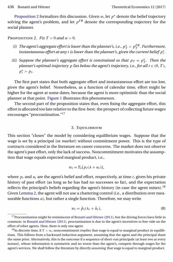
The first part states that both aggregate effort and instantaneous effort are too low,given the agent’s belief. Nonetheless, as a function of calendar time, effort might behigher for the agent at some dates, because the agent is more optimistic than the socialplanner at that point. Figure 1 illustrates this phenomenon.

The second part of the proposition states that, even fixing the aggregate effort, thiseffort is allocated too late relative to the first-best: the prospect of collecting future wagesencourages “procrastination.”17

3. Equilibrium

This section “closes” the model by considering equilibrium wages. Suppose that thewage is set by a principal (or market) without commitment power. This is the type ofcontracts considered in the literature on career concerns. The market does not observethe agent’s past effort, only the lack of success. Noncommitment motivates the assump-tion that wage equals expected marginal product, i.e.,

wt = Et[pt(λ+ ut)]�

where pt and ut are the agent’s belief and effort, respectively, at time t, given his privatehistory of past effort (as long as he has had no successes so far), and the expectationreflects the principal’s beliefs regarding the agent’s history (in case the agent mixes).18

Given Lemma 2, the agent will not use a chattering control (i.e., a distribution over mea-surable functions u), but rather a single function. Therefore, we may write

wt = pt(λt + ut)� (8)

17Procrastination might be reminiscent of Bonatti and Hörner (2011), but the driving forces have little incommon: in Bonatti and Hörner (2011), procrastination is due to the agent’s incentives to free-ride on theeffort of other agents. Here, there is only one agent.

18In discrete time, if T < ∞, noncommitment implies that wage is equal to marginal product in equilib-rium. This follows from a backward induction argument, assuming that the agent and the principal sharethe same prior. Alternatively, this is the outcome if a sequence of short-run principals (at least two at everyinstant), whose information is symmetric and no worse than the agent’s, compete through wages for theagent’s services. We shall follow the literature by directly assuming that wage is equal to marginal product.


where pt and ut denote the belief and anticipated effort at time t, as viewed from themarket.

In equilibrium, expected effort must coincide with actual effort. Note that if theagent deviates, the market will typically hold incorrect beliefs.

Definition 1. An equilibrium is a measurable function u and a wage path w such thatthe following statements hold:

(i) Effort u is a best reply to wages w given the agent’s private belief p, which heupdates according to (1).

(ii) The wage equals the marginal product, i.e., (8) holds for all t.

(iii) Beliefs are correct on the equilibrium path, that is, for every t,

ut = ut�

and therefore, also, pt = pt at all t ∈ [0�T ].

3.1 The continuation game

Here we start by briefly discussing the continuation game in which information is com-plete so that the belief is identically 1. We have so far assumed that the agent receivesan exogenous wage v until the end of the game at T . However, there is no particularreason to assume a bounded horizon for the agent’s career, before or after a success. Forinstance, in Section 4.1, we consider up-or-out arrangements where the agent earns aperpetual wage v if he obtains a breakthrough before the end of the probationary pe-riod T . The agent’s objective (3) is unchanged. Moreover, the unique equilibrium payoffv in the continuation game does not depend on the interpretation for our model. Whilethere might good reasons to treat this continuation payoff after a success as an exoge-nous parameter (after all, the agent may be assigned to another type of task once he hasproved himself), it is easy to endogenize it by solving for the continuation equilibrium.

Lemma 3. Both in the finite and in the infinite continuation game when ω= 1 is commonknowledge, the unique equilibrium payoff is v = λ, and the agent exerts no effort.

The result is clear with a fixed horizon, since the only solution consistent with back-ward induction specifies no effort throughout. It is more surprising that no effort ispossible in equilibrium with an infinite continuation, even without restricting attentionto Markov (or indeed public) equilibria. As we show in the Appendix, this reflects boththe fact that the market behaves myopically and that, in continuous time, the likelihoodratio of the signal that must be used as a trigger for punishment is insensitive to effort.19

19Yet this is not an artifact of continuous time: the same holds in discrete time if the frequency is highenough, as an immediate application of Fudenberg and Levine’s (1994) algorithm. Conversely, if it is lowenough, multiple equilibria can be constructed. The same holds in Holmström’s (1982/1999) model, butthis issue is somewhat obfuscated by his implicit focus on Markov equilibria.


This result is reminiscent of Abreu et al. (1991), but the relationship is superficial, astheir result relies on the lack of identifiability in the monitoring. Here, all signals reflectthe worker’s effort only. Closer is the analysis of Faingold and Sannikov (2011) undercomplete information, where volatility in the Brownian noise prevents any effort to besustained in their model.

3.2 The equilibrium with incomplete information

We now return to the game in which the agent’s type is unknown, and use v as a contin-uation payoff, if only to distinguish it from the arrival rate of a breakthrough. To under-stand the structure of equilibria, consider the following example, illustrated in Figure 1.Suppose that the principal expects the agent to put in the efficient amount of effort,which decreases over time in this example. Accordingly, the wage paid by the firm de-creases as well. The agent’s best-reply, then, is quasi-concave: effort first increases, andthen decreases (see left panel). The agent puts in little effort at the start, as he has noincentive “to kill the golden goose.” Once wages come down, effort becomes more at-tractive, so that the agent increases his effort, before fading out as pessimism sets in.The market’s expectation does not bear out: marginal product is single-peaked. In fact,it would decrease at the beginning if effort was sufficiently flat.

Eventually the agent exerts more effort than the social planner would, because theagent is more optimistic at those times, having worked less in the past (see right panel).Effort is always too low given the actual belief of the agent, but not always given calendartime.

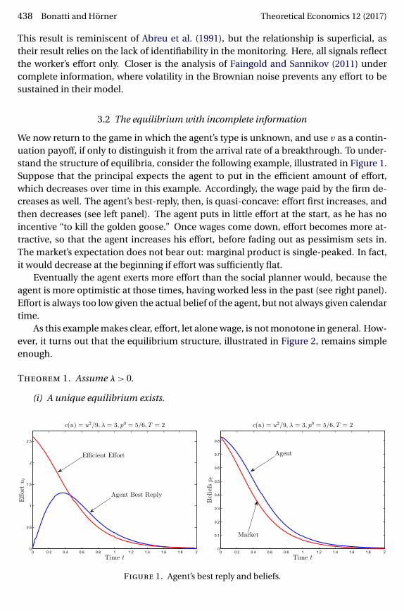
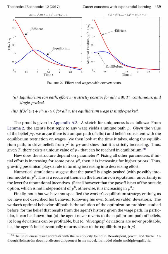
As this example makes clear, effort, let alone wage, is not monotone in general. How-ever, it turns out that the equilibrium structure, illustrated in Figure 2, remains simpleenough.

Theorem 1. Assume λ > 0.

(i) A unique equilibrium exists.

Figure 1. Agent’s best reply and beliefs.


Figure 2. Effort and wages with convex costs.

(ii) Equilibrium (on path) effort ut is strictly positive for all t ∈ [0�T ), continuous, andsingle-peaked.

(iii) If 3c′′(u)+ c′′′(u) ≥ 0 for all u, the equilibrium wage is single-peaked.

The proof is given in Appendix A.2. A sketch for uniqueness is as follows: FromLemma 2, the agent’s best reply to any wage yields a unique path p. Given the valueof the belief pT , we argue there is a unique path of effort and beliefs consistent with theequilibrium restriction on wages. We then look at the time it takes, along the equilib-rium path, to drive beliefs from p0 to pT and show that it is strictly increasing. Thus,given T , there exists a unique value of pT that can be reached in equilibrium.20

How does the structure depend on parameters? Fixing all other parameters, if ini-tial effort is increasing for some prior p0, then it is increasing for higher priors. Thus,growing pessimism plays a role in turning increasing into decreasing effort.

Numerical simulations suggest that the payoff is single-peaked (with possibly inte-rior mode) in p0. This is a recurrent theme in the literature on reputation: uncertainty isthe lever for reputational incentives. (Recall however that the payoff is net of the outsideoption, which is not independent of p0; otherwise, it is increasing in p0.)

Finally, note that we have not specified the worker’s equilibrium strategy entirely, aswe have not described his behavior following his own (unobservable) deviations. Theworker’s optimal behavior off path is the solution of the optimization problem studiedbefore, for the belief that results from the agent’s history, given the wage path. In partic-ular, it can be shown that (a) the agent never reverts to the equilibrium path of beliefs,(b) long deviations can be profitable, but (c) “diverging” deviations are never profitable,i.e., the agent’s belief eventually returns closer to the equilibrium path p∗

t .

20The uniqueness result contrasts with the multiplicity found in Dewatripont, Jewitt, and Tirole. Al-though Holmström does not discuss uniqueness in his model, his model admits multiple equilibria.


3.3 Discussion

The key driver behind the equilibrium structure, as described in Theorem 1, is the strate-gic substitutability between effort at different dates, conditional on lack of success. Ifmore effort is expected tomorrow, wages “tomorrow” will be higher in equilibrium,which depresses incentives, and hence effort “today.” Substitutability between effortat different dates is also a feature of the social planner’s solution, because higher efforttomorrow makes effort today less useful, but wages create an additional channel.

This substitutability appears to be new to the literature on career concerns. As wehave mentioned, in the model of Holmström, the optimal choices of effort today andtomorrow are entirely independent, and because the variance of posterior beliefs is de-terministic with Gaussian signals, the optimal choice of effort is deterministic as well.Dewatripont, Jewitt, and Tirole emphasize the complementarity between expected ef-fort and incentives for effort (at the same date): if the agent is expected to work hard,failure to achieve a high signal will be particularly detrimental to tomorrow’s reputation,which provides a boost to incentives today. Substitutability between effort today and to-morrow does not appear in their model, because it is primarily focused on two periods,and at least three are required for this effect to appear. With two periods only, there areno reputation-based incentives to exert effort in the second (and final) period anyhow.

Conversely, complementarity between expected and actual effort at a given time isnot discernible in our model, because time is continuous. It does, however, appear indiscrete time versions of it, and three-period examples can be constructed that illus-trate both contemporaneous complementarity and intertemporal substitutability of ef-fort levels.

As a result of this novel effect, effort and wage dynamics display original features.Both in Holmström’s and in Dewatripont, Jewitt, and Tirole’s models, the wage is a su-permartingale. Here instead, effort and wages can be first increasing, then decreasing.These dynamics are not driven by the horizon length.21 Neither are they driven by thefact that with two types, the variance of the public belief need not be monotone.22 Thesame pattern emerges in examples with an infinite horizon, and a prior p0 < 1

2 that guar-antees that this variance only decreases over time.

As (6) makes clear, the provision of effort is tied to the capital gain that the agentobtains if he breaks through. Viewed as an integral, this capital gain is too low early on,it increases over time, and then declines again, for a completely different reason. Indeed,this wedge depends on two components: the wage gap, and the impact of effort on the(expected) arrival rate of a success. High initial wages depress the former component,and hence kill incentives to exert effort early on. The latter component declines overtime, so that eventually effort fades out.23

21This is unlike for the social planner, for whom we have seen that effort is nonincreasing with an infinitehorizon, while it is monotone (and possibly increasing) with a finite horizon.

22Recall that in Holmström’s model, this variance decreases (deterministically) over time, which plays animportant role in his results.

23We have assumed—as is usually done in the literature—that the agent does not know his own skill. Theanalysis of the game in which the agent is informed is simple, as there is no scope for signaling. An agentwho knows that his ability is low has no reason to exert any effort, so we focus on the high-skilled agent.Because of the market’s declining belief, the same dynamics arise, and this agent’s effort is single-peaked.


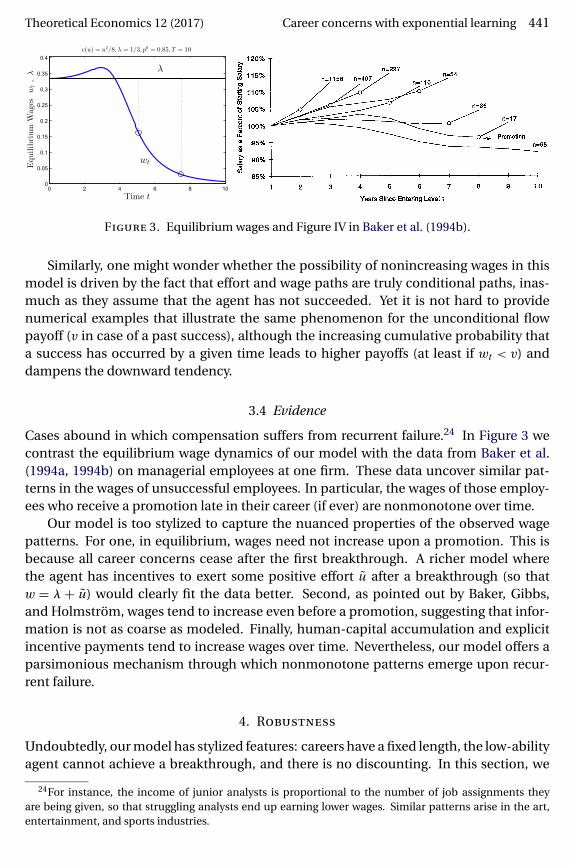
Figure 3. Equilibrium wages and Figure IV in Baker et al. (1994b).

Similarly, one might wonder whether the possibility of nonincreasing wages in thismodel is driven by the fact that effort and wage paths are truly conditional paths, inas-much as they assume that the agent has not succeeded. Yet it is not hard to providenumerical examples that illustrate the same phenomenon for the unconditional flowpayoff (v in case of a past success), although the increasing cumulative probability thata success has occurred by a given time leads to higher payoffs (at least if wt < v) anddampens the downward tendency.

3.4 Evidence

Cases abound in which compensation suffers from recurrent failure.24 In Figure 3 wecontrast the equilibrium wage dynamics of our model with the data from Baker et al.(1994a, 1994b) on managerial employees at one firm. These data uncover similar pat-terns in the wages of unsuccessful employees. In particular, the wages of those employ-ees who receive a promotion late in their career (if ever) are nonmonotone over time.

Our model is too stylized to capture the nuanced properties of the observed wagepatterns. For one, in equilibrium, wages need not increase upon a promotion. This isbecause all career concerns cease after the first breakthrough. A richer model wherethe agent has incentives to exert some positive effort u after a breakthrough (so thatw = λ + u) would clearly fit the data better. Second, as pointed out by Baker, Gibbs,and Holmström, wages tend to increase even before a promotion, suggesting that infor-mation is not as coarse as modeled. Finally, human-capital accumulation and explicitincentive payments tend to increase wages over time. Nevertheless, our model offers aparsimonious mechanism through which nonmonotone patterns emerge upon recur-rent failure.

4. Robustness

Undoubtedly, our model has stylized features: careers have a fixed length, the low-abilityagent cannot achieve a breakthrough, and there is no discounting. In this section, we

24For instance, the income of junior analysts is proportional to the number of job assignments theyare being given, so that struggling analysts end up earning lower wages. Similar patterns arise in the art,entertainment, and sports industries.


briefly consider several variations of our baseline model, and we argue that none ofthese features is critical to our main findings.

4.1 Probationary periods

A probationary period is a distinguishing feature of several professional-services indus-tries. To capture the effect of up-or-out arrangements on reputational incentives, we al-low for a fixed penalty of k≥ 0 for not achieving a success by the deadline T . This mightrepresent diminished future career opportunities to workers with such poor records. Al-ternatively, consider an interpretation of our model with two phases of the agent’s ca-reer: one preceding and one following the “clock” T , which lasts until an exogenousretirement time T ′ > T . Thus, the penalty k represents the difference between the wagethe agent would have earned had he succeeded, and the wage he will receive until hiseventual retirement. Our baseline model with no penalty (k = 0) constitutes a specialcase.

Given a wage function wt , the agent’s problem simplifies to the maximization of∫ T

0

1 −p0

1 −pt[wt − c(ut)− v]dt − 1 −p0

1 −pTk� (9)

Considering the maximization problem (9), there appear to be two drivers of theworker’s effort. First, if the wage falls short of the outside option (i.e., if wt − v is neg-ative), he has an incentive to exert high effort to stop incurring this flow deficit. As inthe baseline model, this is more realistic when the belief p is high. Second, there is anincentive to succeed so as to avoid paying the penalty. This incentive should be mostacute when the deadline looms close, as success becomes unlikely to arrive without ef-fort. Taken together, this suggests an effort pattern that is a convex function of time.However, this ignores that, in equilibrium, the wage reflects the agent’s expected effort.Equilibrium analysis shows that the worker’s effort pattern is, in fact, the exact oppositeof what this first intuition suggests.

In particular, the transversality condition now reads

c′(uT ) = pT · k�as the agent is motivated to avoid the penalty and will exert positive effort until thedeadline. However, the arbitrage equation (7) is unaffected by the transversality con-dition. Hence, equilibrium effort is single-peaked for the same reasons as in Theorem 1.Clearly, for a high enough penalty k, equilibrium effort may be increasing throughout.One might wonder whether the penalty k really hurts the worker. After all, it endowshim with some commitment. It is, in fact, possible to construct examples in which theoptimal (i.e., payoff-maximizing) termination penalty is strictly positive.

4.2 Additive technology and positive discounting

Here, we allow a low-skilled agent to succeed. We do not provide a complete analysis,limiting ourselves to the interaction before the first breakthrough, and considering a


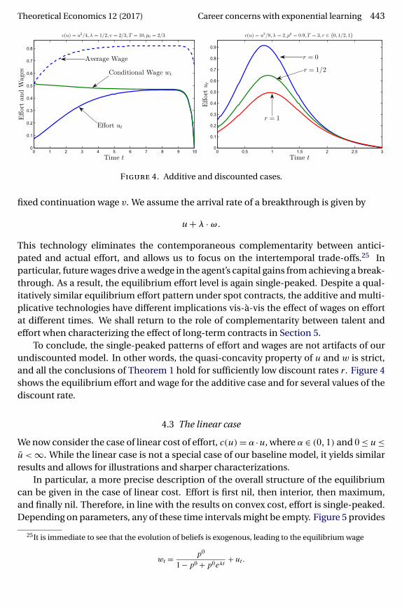
Figure 4. Additive and discounted cases.

fixed continuation wage v. We assume the arrival rate of a breakthrough is given by

u+ λ ·ω�

This technology eliminates the contemporaneous complementarity between antici-pated and actual effort, and allows us to focus on the intertemporal trade-offs.25 Inparticular, future wages drive a wedge in the agent’s capital gains from achieving a break-through. As a result, the equilibrium effort level is again single-peaked. Despite a qual-itatively similar equilibrium effort pattern under spot contracts, the additive and multi-plicative technologies have different implications vis-à-vis the effect of wages on effortat different times. We shall return to the role of complementarity between talent andeffort when characterizing the effect of long-term contracts in Section 5.

To conclude, the single-peaked patterns of effort and wages are not artifacts of ourundiscounted model. In other words, the quasi-concavity property of u and w is strict,and all the conclusions of Theorem 1 hold for sufficiently low discount rates r. Figure 4shows the equilibrium effort and wage for the additive case and for several values of thediscount rate.

4.3 The linear case

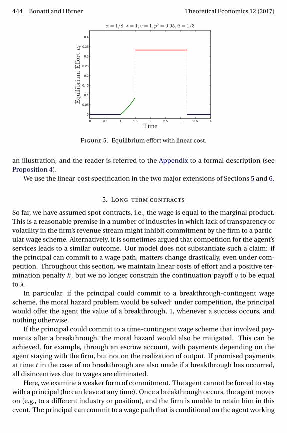
We now consider the case of linear cost of effort, c(u) = α ·u, where α ∈ (0�1) and 0 ≤ u≤u < ∞. While the linear case is not a special case of our baseline model, it yields similarresults and allows for illustrations and sharper characterizations.

In particular, a more precise description of the overall structure of the equilibriumcan be given in the case of linear cost. Effort is first nil, then interior, then maximum,and finally nil. Therefore, in line with the results on convex cost, effort is single-peaked.Depending on parameters, any of these time intervals might be empty. Figure 5 provides

25It is immediate to see that the evolution of beliefs is exogenous, leading to the equilibrium wage

wt = p0

1 −p0 +p0eλt+ ut �


Figure 5. Equilibrium effort with linear cost.

an illustration, and the reader is referred to the Appendix to a formal description (seeProposition 4).

We use the linear-cost specification in the two major extensions of Sections 5 and 6.

5. Long-term contracts

So far, we have assumed spot contracts, i.e., the wage is equal to the marginal product.This is a reasonable premise in a number of industries in which lack of transparency orvolatility in the firm’s revenue stream might inhibit commitment by the firm to a partic-ular wage scheme. Alternatively, it is sometimes argued that competition for the agent’sservices leads to a similar outcome. Our model does not substantiate such a claim: ifthe principal can commit to a wage path, matters change drastically, even under com-petition. Throughout this section, we maintain linear costs of effort and a positive ter-mination penalty k, but we no longer constrain the continuation payoff v to be equalto λ.

In particular, if the principal could commit to a breakthrough-contingent wagescheme, the moral hazard problem would be solved: under competition, the principalwould offer the agent the value of a breakthrough, 1, whenever a success occurs, andnothing otherwise.

If the principal could commit to a time-contingent wage scheme that involved pay-ments after a breakthrough, the moral hazard would also be mitigated. This can beachieved, for example, through an escrow account, with payments depending on theagent staying with the firm, but not on the realization of output. If promised paymentsat time t in the case of no breakthrough are also made if a breakthrough has occurred,all disincentives due to wages are eliminated.

Here, we examine a weaker form of commitment. The agent cannot be forced to staywith a principal (he can leave at any time). Once a breakthrough occurs, the agent moveson (e.g., to a different industry or position), and the firm is unable to retain him in thisevent. The principal can commit to a wage path that is conditional on the agent working


for her firm. Thus, wages can only be paid in the continued absence of a breakthrough.Until a breakthrough occurs, other firms, who are symmetrically informed (they observethe wages paid by all past employers), compete by offering wage paths. The same dead-line applies to all wage paths, i.e., the tenure clock is not reset. For instance, the deadlinecould represent the agent’s retirement age, so that switching firms does not affect thehorizon.

We write the principal’s problem as that of maximizing the agent’s welfare subject toconstraints. We take it as an assumption that competition among principals leads to themost preferred outcome of the agent, subject to the firm breaking even.

Formally, we solve the following optimization problem P .26 The principal choosesu : [0�T ] → [0� u] and w : [0�T ] → R+, integrable, to maximize W (0�p0), where, for anyt ∈ [0�T ],

W (t�pt) := maxw�u

∫ T

t

1 −pt

1 −ps(ws − v − αus)ds − k

1 −pt

1 −pT�

such that, given w, the agent’s effort is optimal,

u = arg maxu

∫ T

t

1 −pt

1 −ps(ws − v− αus)ds − k

1 −pt

1 −pT�

and the principal offers as much to the agent at later times than the competition couldoffer at best, given the equilibrium belief,

∀τ ≥ t:∫ T

τ

1 −pτ

1 −ps(ws − v − αus)ds − k

1 −pτ

1 −pT≥W (τ�pτ); (10)

finally, the firm’s profit must be nonnegative,

0 ≤∫ T

t

1 −pt

1 −ps(ps(λ+ us)−ws)ds�

Note that competing principals are subject to the same constraints as the principal un-der consideration: because the agent might ultimately leave them as well, they can offerno better than W (τ�pτ) at time τ, given belief pτ. This leads to an “infinite regress”of constraints, with the value function appearing in the constraints themselves. To beclear, W (τ�pτ) is not the continuation payoff that results from the optimization prob-lem, but the value of the optimization problem if it started at time τ.27 Because of theconstraints, the solution is not time consistent, and dynamic programming is of little

26We are not claiming that this optimization problem yields the equilibrium of a formal game, in whichthe agent could deviate in his effort scheme, leave the firm, and competing firms would have to form beliefsabout the agent’s past effort choices, etc. Given the well known modeling difficulties that continuous timeraises, we view this merely as a convenient shortcut. Among the assumptions that it encapsulates, note thatthere is no updating based on an off-path action (e.g., switching principals) by the agent.

27Harris and Holmström (1982) impose a similar condition in a model of wage dynamics under incom-plete information. However, because their model abstracts from moral hazard, constraint (10) reduces to anonpositive continuation profit condition.


help. Fortunately, this problem can be solved, as shown in Appendix A.3, at least as longas u and v are large enough. Formally, we assume that

u≥(

v

αλ− 1

)v− λ and v ≥ λ(1 + k)�28 (11)

Before describing its solution, let us provide some intuition. Future payments dodepress incentives, but their timing is irrelevant if ω = 0, as effort makes no differencein that event anyhow. Hence, the impact on incentives can be evaluated conditional onω = 1. However, in that event, remote payments are unlikely to be collected anyhow, asa success is likely to have occurred by then. This dampens the detrimental impact ofsuch payments on incentives. The benefit from postponing future payments as muchas possible comes from this distinction: the rate at which they are discounted from theprincipal’s point of view is not the same as the one used by the agent when determininghis optimal effort, because of this conditioning.

More precisely, recall the first-order condition (6) that determines the agent’s effort.Clearly, the lower the future total wage bill, the stronger the agent’s incentives to exerteffort, which is inefficiently low in general. Now consider two times t < t ′: to providestrong incentives at the later time t ′, it is best to frontload any promised payment totimes before t ′, as such payments will no longer matter at that time. Ideally, the princi-pal would pay what he owes up front, as a “signing bonus.” Of course, this violates theconstraint (10), as an agent left with no future payments would leave right after cashingin the signing bonus.

From the perspective of incentives at the earlier time t, however, backloadingpromised payments can be beneficial. To see this formally, note that the coefficient ofthe wage ws , s > t, in (6) is the likelihood ratio ps/(1 −ps), as explained before. Up to thefactor (1 −pt), we obtain

(1 −pt)ps

1 −ps= P[ω = 1|τ ≥ s]P[ω = 1] = P[ω = 1 ∩ τ ≥ s];

that is, effort at time t is affected by wage at time s > t inasmuch as time s is reached andthe state is 1: otherwise effort plays no role anyhow.

In terms of the firm’s profit, the coefficient placed on the wage at time s (see (10)) is

P[τ ≥ s]�i.e., the probability that this wage is paid (or collected). Thus, if the firm wishes to back-load payments and break even, the nominal value of those payments must be increased,as a breakthrough might occur until then, which would void them; but the probabilitythat these payments must be made decreases in the same proportion. Thus, what mat-ters for incentives is not the probability that time s is reached, but the fact that reachingthose later times is indicative of state 0.

In particular, because players grow more pessimistic over time, the coefficient onfuture wages in the agent’s first-order condition (6) decreases faster than in the firm’s

28We do not know whether these assumptions are necessary for the result.


profits. Hence, later payments depress current incentives less than earlier payments:backloading payments is good for incentives at time t.

To sum up: from the perspective of time t, backloading payments is useful; from thepoint of view of t ′ > t, it is detrimental, but frontloading is constrained by (10). Note that,as T → ∞, the planner’s solution tends to the agent’s best response to a wage of w = 0.Hence, the firm can approach first best by promising a one-time payment arbitrarily farin the future (and wages equal to marginal product thereafter). This would be almostas if w = 0 for the agent’s incentives, and would induce efficient effort. The lump-sumpayment would then be essentially equal to p0/(1 −p0).

Note finally that, given the focus on linear cost, there is no benefit in giving the agentany “slack” in his incentive constraint at time t; otherwise, by frontloading slightly futurepayments, incentives at time t would not be affected, while incentives at later timeswould be enhanced. Hence, the following result should come as no surprise.

Theorem 2. The following statement is a solution to the optimization problem P , forsome t ∈ [0�T ]. Maximum effort is exerted up to time t, and zero effort is exerted after-ward. The wage is equal to v− αλ up to time t, so that the agent is indifferent between alllevels of effort up to then, and it is 0 for all times s ∈ (t�T ); a lump sum is paid at time T .29

The proof is given in Appendix A.3, and it involves several steps: we first conjecturea solution in which effort is first full (and the agent is indifferent), then nil; we relax theobjective in program P to maximization of aggregate effort, and relax constraint (10)to a nonpositive continuation profit constraint; we verify that our conjecture solves therelaxed program, and finally that it also solves the original program. In the last step weshow that (a) given the shape of our solution, maximizing total effort implies maximizingthe agent’s payoff, and (b) the competition constraint (10) is slack at all times t > 0.

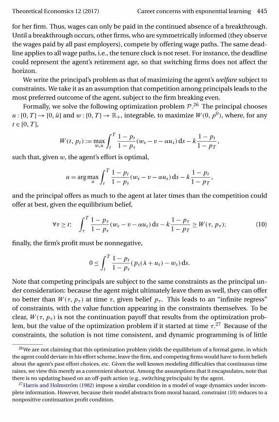
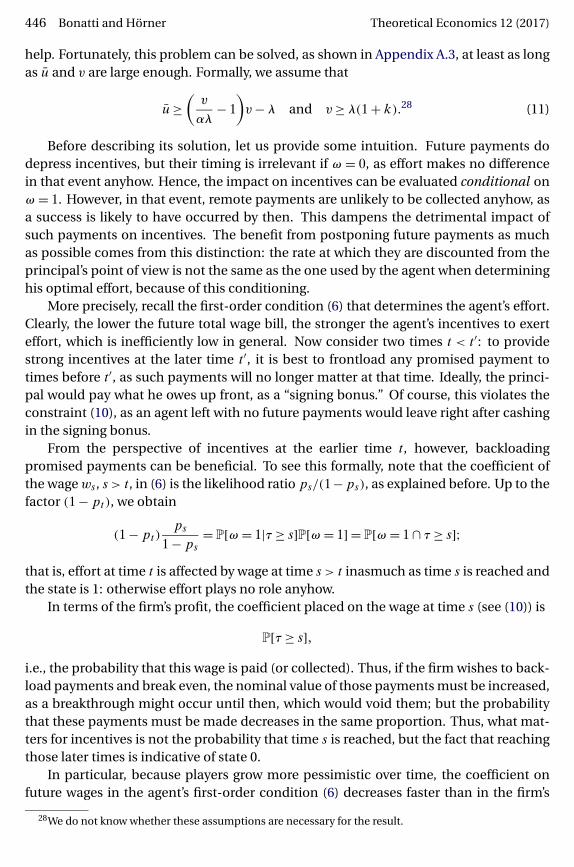
Hence, under one-sided commitment, high effort might be exerted throughout. Thishappens if T is short and k > 0. When u is high enough (precisely, when (11) holds),the agent produces revenue that exceeds the flow wage collected as time proceeds: theliability recorded by the principal grows over time, shielding it from the threat of com-petition. This liability will eventually be settled via a lump-sum payment at time T thatcan be interpreted as severance pay. If the horizon is longer or k = 0, the lump sumwipes out incentives close to the deadline, and effort is zero in a terminal phase. Thus, aphase with no effort exists if and only if the deadline is long enough. The two cases areillustrated in Figure 6.

As mentioned, all these results are proved for the case of linear cost. It is all themore striking that the result obtains in this “linear” environment. Indeed, rigidity andseverance pay are usually attributed to risk aversion by the agent (see Azariadis 1975,Holmström 1983, Harris and Holmström 1982, Thomas and Worrall 1988).30 Our model

29The wage path that solves the problem is not unique in general.30In Thomas and Worrall (1988), there is neither incomplete information nor moral hazard. Instead,

the spot market wage is treated as an exogenous independent and identically distributed (i.i.d.) pro-cess (though Thomas and Worrall do not require risk aversion; with market power and commitment,backloading improves incentives). Holmström (1983) is a two-period example. As mentioned above,


Figure 6. Wages and effort under commitment for two horizon lengths.

with commitment and competition provides an alternative rationale. To sum up, witha long horizon, commitment alleviates the unavoidable delay in effort provision thatcomes with compensating a worker for persistent failure by backloading compensation.

6. Observable effort

The inability to contract on effort might be attributable to the subjectivity in its mea-surement rather than to the impossibility of monitoring it. To understand the role of ob-servability of effort, we assume here that effort is observed. Because effort is monitored,the firm and agent beliefs coincide on- and off-path. The flow wage is given by

wt = pt(λ+ ut)�

where pt is the belief and ut is expected effort. We assume linear cost. The agentmaximizes

V (p0�0) :=∫ T

0

1 −p0

1 −pt[pt(λ+ ut)− αut − v]dt − k

1 −p0

1 −pT�

In contrast to (3), the firm’s revenue is no longer a function of time only, as effort affectsfuture beliefs, thus wages. Hence, effort is a function of both t and p. We focus onequilibria in Markov strategies

u : [0�1] × [0�T ] → [0� u]�such that u(p� t) is upper semicontinuous and the value function V (p� t) is piecewisedifferentiable.31

Harris and Holmström (1982) has incomplete information about the worker’s type, but no moral hazard.Hence, the logic of rigidity and backloading that appears in these models is very different from ours, drivenby optimal incentive provision under incomplete information.

31That is, there exists a partition of [0�1] × [0�T ] into closed Si with nonempty interior, such that V

is differentiable on the interior of Si, and the intersection of any Si, Sj is either empty or a smooth one-dimensional manifold.


Lemma 4. Fix a Markov equilibrium. Suppose the agent exerts strictly positive effort attime t (givenp). Then the equilibrium specifies strictly positive effort at all times t ′ ∈ (t�T ].

Thus, in any equilibrium involving extremal effort levels only, there are at most twophases: the worker exerts no effort and then full effort. This is the opposite of the sociallyoptimal policy, which frontloads effort (see Lemma 1). The agent can only be trusted toput in effort if his “back is to the wall,” so that effort remains optimal at any later time,no matter what he does; if the market paid for effort, yet the agent was expected to letup later on, then he would gain by deviating to no effort, pocketing the high wage inthe process; because such a deviation makes everyone more optimistic, it would onlyincrease his incentives to exert effort (and so his wage) at later times.

This does not imply that the equilibrium is unique, as the next theorem establishes.

Theorem 3. Given T > 0, there exists continuous, distinct, nonincreasing¯p� p : [0�T ] →

[0�1] (with¯pt ≤ pt with equality if t = T ) such that the following statements hold:

(i) All Markov equilibria involve maximum effort if pt > pt .

(ii) All Markov equilibria involve no effort if pt ≤¯pt .

(iii) These bounds are tight: there exists a Markov equilibrium in which effort is either0 or u if and only if p is below or above

¯p (resp., p).

The proof of Theorem 3 provides a description of these belief boundaries. Theseboundaries might be as high as 1, in which case effort is never exerted at that time: in-deed, there is t∗ (independent of T ) such that effort is zero at all times t < T − t∗ (ifT > t∗). The threshold

¯p is decreasing in the cost α, and increasing in v and k. Con-

sidering the equilibrium with maximum effort—the agent works more—the more de-sirable success is.32

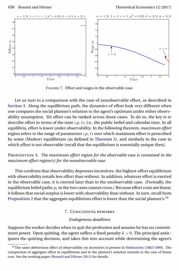
Figure 7 illustrates these dynamics. In any extremal equilibrium,wages decrease over time, except for an upward jump when effort jumps up to u. In theinterior-effort equilibrium described in the proof (in which effort is continuous through-out), wages decrease throughout. Further comparative statics are given in the Appendix.

Equilibrium multiplicity has a simple explanation. Because the firm expects effortonly if the belief is high and the deadline is close, such states (belief and times) are desir-able for the agent, as the higher wage more than outweighs the effort cost. Yet low effortis the best way to reach those states, as effort depresses beliefs: hence, if the firm expectsthe agent to shirk until a high boundary is reached (in (p� t) space), the agent has strongincentives to shirk to reach it; if the firm expects shirking until an even higher boundary,this would only reinforce this incentive.33

32While the equilibria achieving the result in part (iii) of Theorem 3 (say, ¯σ and σ) provide upper andlower bounds on equilibrium effort (in the sense of parts (i) and (ii)), these equilibria are not the only ones.Other equilibria exist that involve only extremal effort, with a switching boundary in between

¯p and p; there

are also equilibria in which interior effort levels are exerted at some states.33Non-Markov equilibria exist. Defining them in our environment is problematic, but it is clear that

threatening the agent with reversion to the Markov equilibrium σ provides incentives for effort extendingbeyond the high-effort region defined by ¯σ—in fact, beyond the high-effort region in the unobservablecase. The planner’s solution remains out of reach, as punishments are restricted to beliefs below

¯p.


Figure 7. Effort and wages in the observable case.

Let us turn to a comparison with the case of nonobservable effort, as described inSection 3. Along the equilibrium path, the dynamics of effort look very different whenone compares the social planner’s solution to the agent’s optimum under either observ-ability assumption. Yet effort can be ranked across those cases. To do so, the key is todescribe effort in terms of the state (p� t), i.e., the public belief and calendar time. In allequilibria, effort is lower under observability. In the following theorem, maximum effortregion refers to the range of parameters (p� t) over which maximum effort is prescribedby some (Markov) equilibrium (as defined in Theorem 3), and similarly in the case inwhich effort is not observable (recall that the equilibrium is essentially unique then).

Proposition 3. The maximum effort region for the observable case is contained in themaximum effort region(s) for the nonobservable case.

This confirms that observability depresses incentives: the highest-effort equilibriumwith observability entails less effort than without. In addition, whatever effort is exertedin the observable case, it is exerted later than in the unobservable case. (Formally, theequilibrium belief paths pt in the two cases cannot cross.) Because effort costs are linear,it follows that social surplus is lower with observability than without. In turn, recall fromProposition 2 that the aggregate equilibrium effort is lower than the social planner’s.34

7. Concluding remarks

Endogenous deadlines

Suppose the worker decides when to quit the profession and assume he has no commit-ment power. Upon quitting, the agent suffers a fixed penalty k > 0. The principal antic-ipates the quitting decision, and takes this into account while determining the agent’s

34The same deleterious effect of observability on incentives is present in Holmström (1982/1999). Thecomparison of aggregate effort in equilibrium and in the planner’s solution extends to the case of linearcost. See the working paper (Bonatti and Hörner 2013) for details.


equilibrium effort and, therefore, the wage he should be paid. For simplicity, we adoptpassive beliefs. That is, if the agent is supposed to drop out at some time but fails todo so, the principal does not revise his belief regarding past effort choices, ascribing thefailure to quit to a mistake (i.e., he expects the agent to quit at the next instant).

It is easy to show that endogenous deadlines do not affect the pattern of effort andwage: the wage is decreasing at the end (but not necessarily at the beginning); effort andwages are single-peaked. Furthermore, the belief at the deadline is too high relative tothe social planner’s at the first-best deadline.35 How about if the worker could committo the deadline (but still not to effort levels)? The optimal deadline with commitment isset so as to increase aggregate effort and therefore wages. Numerical simulations sug-gest this requires decreasing the deadline, so as to provide stronger incentives througha larger penalty, i.e., to make high effort levels credible.

Multiple breakthroughs

Suppose that one success does not resolve all uncertainty. Specifically, there are threestates and two consecutive projects. The first project can be completed if and only ifthe agent is not bad (i.e., if he is good or great). If the first project is completed, anobservable event, the agent tackles the second, which can be completed only if the agentis great. Such an extension can be solved by backward induction. Once the first project iscompleted, the continuation game reduces to the game of Section 3. The value functionof this problem then serves as a continuation payoff to the first stage. While this valuefunction cannot be solved in closed form, it is easy to derive the solution numerically.The same pattern as in our baseline model emerges: effort is single-peaked, and, as aresult, wages can be first decreasing and then single-peaked.

Furthermore, effort at the start of the second project is also single-peaked as a func-tion of the time at which this project is started (the later it is started, the more pessimisticthe agent at that stage, though his belief has obviously jumped up given the success).

Learning by doing

Memorylessness is a convenient but stark property of the exponential distribution. Itimplies that past effort plays no role in the probability of instantaneous breakthrough.In many applications, agents learn from the past not only about their skill levels, butabout the best way to achieve a breakthrough. While a systematic analysis of learningby doing is beyond the scope of this paper, we can gain some intuition from numericalsimulations. We assume the evolution of human capital is given by

zt = ut − δzt� z0 = 0�

while its productivity is

ht = ut + ρzφt �

35Having the worker quit when it is best for him (without commitment to the deadline) reinforces ourcomparison between observable and nonobservable effort. See the working paper (Bonatti and Hörner2013) for details.


Not surprisingly, simulations suggest that the main new feature is a spike of effort at thebeginning, whose purpose is to build human capital. This spike might lead to decreasinginitial effort, before it becomes single-peaked, though this need not be the case. Beyondthis new twist, features from the baseline model appear quite robust.

Appendix

Throughout this appendix, we shall use the log-likelihood ratio

xt := ln1 −pt

pt

of state ω = 0 vs. ω = 1. We set x0 := ln(1 −p0)/p0. Note that x increases over time and,given u, follows the ordinary differential equation (O.D.E.)

xt = λ+ ut�

with x0 = x0. We shall also refer to xt as the belief, hoping that this will create noconfusion.

We start by explaining how the objective function can be derived as the limit of adiscounted version of our problem. Suppose that Wt is the value of a success at timet, corresponding to earning the flow wage v until the end of the game at T . Given thediscount rate r, we have

Wt = v

r(1 − e−r(T−t))�

and hence the agent’s ex ante payoff V0 is given by

V0 =∫ T

0e−rt 1 + e−xt

1 + e−x0

(xt

1 + extWt +wt − c(ut)

)dt�

Integrating the first term by parts, we obtain

V0 − 11 + ex0

v

r(1 − e−rT ) =

∫ T

0e−rt 1 + e−xt

1 + e−x0

(wt − c(ut)− v

1 + ext

)dt�

so that as r → 0, we obtain

(1 + e−x0)V0 − e−x0vT =∫ T

0(1 + e−xt )

(wt − c(ut)− v

1 + ext

)dt�

Similarly, one can show the social planner’s payoff is given by

(1 + e−x0)V0 − e−x0(vT + 1)= −∫ T

0(1 + e−xt )

(c(ut)+ v

1 + ext

)dt − e−xT �


A.1 Proofs for Section 2

Proof of Lemma 1. Existence and uniqueness of a solution follow as a special case ofLemma 2, when w = 0 identically (the transversality condition must be adjusted). To seethat the social planner’s problem is equivalent to this, note that the “revenue” term ofthe social planner’s objective satisfies∫ T

0(1 + e−xt )

λ+ ut

1 + extdt =

∫ T

0xte

−xt dt = e−x0 − e−xT �

and so this revenue only affects the necessary conditions through the transversality con-dition at T .

The social planner maximizes∫ T

0(1 + e−xt )

(λ+ ut

1 + ext− c(ut)− v

)dt� s.t. xt = λ+ ut�

We note that the maximization problem cannot be abnormal, since there is no restric-tion on the terminal value of the state variable. See Seierstad and Sydsæter (1987,Chapter 2, Note 5). The same holds for all optimization problems considered below.From now on, it will be understood that statements about derivatives only hold almosteverywhere.

Let γt be the costate variable. The Hamiltonian for this problem is

H(x�u�γ� t) = e−xt (λ+ ut)− (1 + e−xt )(v + c(ut))+ γt(λ+ ut)�

Applying Pontryagin’s theorem (and replacing the revenue term by its expression interms of xt and x0, as explained above) yields as necessary conditions

γt = −e−x(c(u)+ v)� γt = (1 + e−xt )c′(ut)�

Differentiate the second expression with respect to time, and use the first one to obtain

u = (λ+ u)c′(u)− c(u)− v

c′′(u)(1 + ex)� (12)

in addition to x= λ+ u (time subscripts will often be dropped for brevity). Let

φ(u) := (λ+ u)c′(u)− c(u)− v�

Note that φ(0) = −v < 0, and φ′(u) = (λ+u)c′′(u) > 0, and so φ is strictly increasing andconvex. Let u∗ ≥ 0 be the unique solution to

φ(u∗)= 0�

and so φ is negative on [0�u∗] and positive on [u∗�∞). Accordingly, u < u∗ ⇒ u < 0,u = u∗ ⇒ u = 0, and u > u∗ ⇒ u > 0. Given the transversality condition

(1 + exT )c′(uT ) = 1�


we define

xT (x0)= 1

λ+ u∗

[ln

(1

c′(u∗)− 1

)− x0

]�

and so effort is decreasing throughout if xT > xT (x0), increasing throughout if

xT < xT (x0), and equal to u∗ throughout otherwise.

Finally, we establish that the belief xT at the deadline is increasing in T . Note thatthe necessary conditions define a vector field (u� x), with trajectories that only dependon the time left before the deadline and the current belief. Because trajectories do notcross (in the plane (−τ�x), where τ is time to go and x is the belief), and belief x canonly increase with time, if we compare two trajectories starting at the same level x0, theone that involves a longer deadline must necessarily involve as high a terminal belief xas the other (as the deadline expires). �

Proof of Lemma 2. We address the two claims in turn.Existence. Note that the state equation is linear in the control u, while the objective’s

integrand is concave in u. Hence the set N(x�U� t) is convex (see Seierstad and Sydsæter1987, Chapter 2, Theorem 8). Therefore, the Filippov–Cesari existence theorem applies(see Cesari 1983).

Uniqueness. We can write the objective, up to constant terms, as∫ T

0(1 + e−xt )(wt − v − c(ut))dt�

or, using the likelihood ratio lt := pt/(1 −pt) > 0,

J(l) :=∫ T

0(1 + lt)(wt − v − c(ut))dt�

Suppose that there are two distinct optimal trajectories l1 and l2, with associatedcontrols u1 and u2. Assume without loss of generality that

l1�t < l2�t for all t ∈ (0�T ]�

We analyze the modified objective function

J(l) :=∫ T

0(1 + lt)(wt − v − ct (ut))dt�

in which we replace the cost function c(ut) with

ct (u) :={αtu if u ∈ [min{u1�t � u2�t}�max{u1�t � u2�t}]c(u) if u /∈ [min{u1�t � u2�t}�max{u1�t � u2�t}],

where

αt := max{c(u1�t)� c(u2�t)} − min{c(u1�t)� c(u2�t)}max{u1�t � u2�t} − min{u1�t � u2�t} �


(If u1�t = u2�t =: ut for some t, set αt equal to c′(ut).) Because ct (u) ≥ c(u) for all t, u, thetwo optimal trajectories l1 and l2, with associated controls u1 and u2, are optimal for themodified objective J(l) as well. Furthermore, J(l1) = J(l1) and J(l2) = J(l2).

We construct a feasible path lt and its associated control ut ∈ [min{u1�t � u2�t}�max{u1�t � u2�t}] that attains a higher payoff J(l) and therefore a strictly higher payoff J(l).Suppose ut ∈ [u1�t � u2�t] for all t. Letting gt := wt − v + αλ − αt , we rewrite the modifiedobjective as ∫ T

0ltgt dt −

∫ T

0αt ln lt dt + αT lT + αT ln lT + constant�

We now consider a continuous function εt ≥ 0 and two associated variations on thepaths l1 and l2:

l′1�t := (1 − εt)l1�t + εtl2�t

l′2�t := (1 − εt)l2�t + εtl1�t �

Because l1 and l2 are optimal, for any εt it must be the case that

J(l1)− J(l′1) ≥ 0

J(l2)− J(l′2) ≥ 0�

We can write these payoff differences as∫ T

0εt(l1�t − l2�t)gt dt +

∫ T

0αtεt

l2�t − l1�tl1�t

dt

+ αTεT (l1�T − l2�T )− αTεTl2�T − l1�T

l1�T+ o(‖ε‖)≥ 0

∫ T

0εt(l2�t − l1�t)gt dt +

∫ T

0αtεt

l1�t − l2�tl2�t

dt

+ αTεT (l2�T − l1�T )− αTεTl1�T − l2�T

l2�T+ o(‖ε‖)≥ 0�

Letting

ρt := l1�t/ l2�t < 1 for all t > 0�

we can sum the previous two conditions (up to the second-order term). Finally, inte-grating by parts, we obtain the condition,∫ T

0

[εt

εt

(2 − ρt − 1

ρt

)+ ρt

1 − ρ2t

ρ2t

]αtεt dt ≥ 0�

which must hold for all εt . Using the fact that ρ= ρ(u2 − u1) we have∫ T

0

[− εt

εt(1 − ρt)+ (u2�t − u1�t)(1 + ρt)

]αtεt

1 − ρt

ρtdt ≥ 0� (13)


We now identify bounds on the function εt so that both variations l′1 and l′2 are feasi-ble and their associated controls lie in [min{u1�t � u2�t}�max{u1�t � u2�t}] for all t. Considerthe identities

l′1 = −l′1�t(λ+ ut)≡ εt(l2�t − l1�t)− λl′1�t − (1 − εt)u1�t l1�t − εtu2�t l2�t

l′2 = −l′2�t(λ+ ut)≡ εt(l1�t − l2�t)− λl′2�t − εtu1�t l1�t − (1 − εt)u2�t l2�t �

We therefore have the expressions for the function ε/ε associated with each variation:

εt

εt= (u1�t − ut)

1−εtεt

l1�t + l2�t(u2�t − ut)

l2�t − l1�t(14)

εt

εt= (u1�t − ut)l1�t + 1−εt

εtl2�t(u2�t − ut)

l1�t − l2�t� (15)

In particular, whenever u2�t > u1�t , the condition

εt

εt∈

[−1 − εt

εt

l2�t(u2�t − u1�t)

l2�t − l1�t�l1�t(u2�t − u1�t)

l2�t − l1�t

]

ensures the existence of two effort levels ut ∈ [u1�t � u2�t] that satisfy conditions (14) and(15) above. Similarly, whenever u1�t > u2�t , we have the bound

εt

εt∈

[− l1�t(u1�t − u2�t)

l2�t − l1�t�

1 − εt

εt

l2�t(u2�t − u1�t)

l2�t − l1�t

]�

Note that εt/εt = 0 is always contained in both intervals.Finally, because ρ0 = 1 and ρt < 1 for all t > 0, we must have u1�t > u2�t for t ∈ [0� t∗)

with t∗ > 0. Therefore, we can construct a path εt that satisfies

(u2�t − u1�t)1 + ρt

1 − ρt<

εt

εt< 0 ∀t ∈ [0� t∗)�

with ε0 > 0 and εt ≡ 0 for all t ≥ t∗. Substituting into condition (13) immediately yields acontradiction. �

Proof of Proposition 1. Applying Pontryagin’s theorem yields (7). It also follows thatthe effort and belief (x�u) trajectories satisfy

c′′(u)(1 + ex)u = (λ+ u)c′(u)− c(u)+wt − v (16)

x= λ+ u�

with boundary conditions

x0 = x0

uT = 0� (17)


Differentiating (16) further, we obtain

(c′′(u)(1 + ex))2u′′t

= ((λ+ u)c′′(u)u′t +w′

t )c′′(u)(1 + ex)

− ((λ+ u)c′(u)+wt − c(u)− v)(c′′′(u)u′t (1 + ex)+ ex(λ+ u)c′′(u))�

Thus, when u′t = 0, we obtain

c′′(u)(1 + ex)u′′t =w′

t �

Combined with the transversality condition (17) and our assumption that the first-ordercondition holds at all times, this immediately implies the conclusion. �

Proof of Proposition 2. From (12) we obtain the expression

u′(x) = (λ+ u)c′(u)− c(u)− v

c′′(u)(1 + ex)(λ+ u)�

which must hold for the optimal trajectory (in the (x�u) plane) for the social planner.Denote this trajectory xFB. The corresponding law of motion for the agent’s optimumtrajectory x∗ given w is

1x′(u)

= (λ+ u)c′(u)− c(u)+wt − v

c′′(u)(1 + ex)(λ+ u)�

(Note that, not surprisingly, time matters.) This implies that (in the (x�u) plane) thetrajectories xFB and x∗ can only cross one way, if at all, with x∗ being the flatter one. Yetthe (decreasing) transversality curve of the social planner, implicitly given by

(1 + exT )c′(uT ) = 1�

lies above the (decreasing) transversality curve of the agent, which is defined by uT = 0.Suppose now that the trajectory xFB ends (on the transversality curve) at a lower be-

lief xFBT than x∗: then it must be that effort u was higher throughout along that trajectorythan along x∗ (since the latter is flatter, xFB must have remained above x∗ throughout).But since the end value of the belief x is simply x0 + ∫ T

0 us ds, this contradicts xFBT < x∗T .

It follows that for a given x, the effort level u is higher for the social planner.The same reasoning implies the second conclusion: if xFBT = x∗

T , so that total effortis the same, yet the trajectories can only cross one way (with x∗ being flatter), it followsthat x∗ involves lower effort first, and then larger effort, i.e., the agent backloads effort. �


First, we describe and prove the omitted characterization in the case of linear cost.Proposition 4 describes the equilibrium in the linear case

Proposition 4. With linear cost, any equilibrium path consists of at most four phases,for some 0 ≤ t1 ≤ t2 ≤ t3 ≤ T :


(i) During [0� t1], no effort is exerted.

(ii) During (t1� t2], effort is interior, i.e., ut ∈ (0� u).

(iii) During (t2� t3], effort is maximal.

(iv) During (t3�T ], no effort is exerted.

Any of these intervals might be empty.36

Proof of Proposition 4. We prove the following statements:

1. If there exists t ∈ (0�T ) such that φt > 0, then there exists t ′ ∈ [t�T ] such that us = u

for s ∈ [t� t ′] and us = 0 for s ∈ (t ′�T ].2. If there exists t ∈ (0�T ) such that φt < 0, then either us = 0 for all s ∈ [t�T ] or us = 0

for all s ∈ [0� t].This implies the desired decomposition. For the first part, note that either us = u forall s > t or there exists t ′′ such that both φt ′′ > 0 (so in particular ut ′′ = u) and φt ′′ < 0.Because pt decreases over time and us ≤ ut ′′ for all s > t ′′, it follows that ws < wt ′′ , and soφs < φt ′′ < 0. Hence φ can cross 0 only once for values above t, establishing the result.For the second part, note that either us = 0 for all s ≥ t or there exists t ′′ ≥ t such thatφt ′′ < 0 (so in particular ut ′′ = 0) and φt ′′ > 0. Because pt decreases over time and us ≥ ut ′′

for all s < t ′′, it follows that ws ≥wt ′′ , and so φs > φt ′′ > 0. For all s < t ′′, φs < 0 and φs > 0.Hence, us = 0 for all s ∈ [0� t]. �

Proof of Lemma 3. We can apply the continuous-time average cost optimality equa-tion for multichain processes (see, e.g., Theorem 5.7 of Guo and Hernández-Lerma2009). To verify their Assumption 5.4, we introduce a discount rate r (or a sequencethereof, tending to 0). Assume a public randomization device, which, given the neg-ative result, is irrelevant. This is a game between a long-run player—the worker—and a sequence of short-run players—the market. Monitoring has a product structure,since wages are perfectly observed while the occurrence of breakthroughs relies on theworker’s action only. It follows that attention can be restricted to strategies that dependon the public history only. Hence, there is a well defined highest and lowest equilibriumpayoff for the agent, independent of the entire history. Let us denote by v ≥ ¯v the corre-sponding average values. Given the randomization device, attention can be restricted tothe strategies that achieve these values. Note that ¯v = λ: never exerting any effort is anoption, and guarantees λ as a payoff; conversely, if the market never expects any effort,not exerting any is a best reply. To achieve v, it is best to promise v as continuation utilityif a breakthrough occurs, and threaten with reversion to ¯v if no such breakthrough ob-tains with the minimum probability necessary to induce the desired level of effort. Let γdenote the rate at which reversion occurs in the absence of breakthroughs. It must hold

36Here and elsewhere, the choices at the extremities of the intervals are irrelevant, and our specificationis arbitrary in this respect.


that γ = O(dt), because the probability that a breakthrough occurs is of order dt. Hence,γ is at most zdt, for some z > 0, but then it holds that

v = maxu≥0

{r dt(w− c(u))+ (1 − r dt)

(v − (1 − (λ+ u)dt)zdt · (v − ¯v)

)} + o(dt)�

where w is the wage paid to the worker (equal to his expected output in the best equilib-rium). Clearly the optimum effort is 0, as the impact of effort on the probability of pun-ishment is of second order, while the cost is of first order. Verification of Theorem 5.7 ofGuo and Hernández-Lerma (2009) is immediate. �

Proof of Theorem 1. We start by establishing that equilibrium effort and wages arestrictly positive (for t < T ) and single-peaked. We then use these properties to proveuniqueness and existence.

Positive effort. We know from transversality that uT = 0. Furthermore, the arbitrageequation (7) implies that whenever ut = 0 in equilibrium, the derivative of effort is givenby

c′′(ut)ut = ptλ(pt − 1) < 0�

Because ut is continuous on [0�T ], it then follows that ut > 0 for all t < T .Single-peakedness. Single-peakedness of effort is almost immediate. Substituting

the equilibrium expression wt = (λ + ut)/(1 + ext ) in the boundary value problem (16).Differentiating u′

t further, we obtain

u′t = 0 ⇒ c′′(u)(1 + e−x)u′′

t = −(wt)2�

which implies that the function u is at most first increasing then decreasing.We now argue that the wage is single-peaked. In terms of x, the wage is given by

w(x) = λ+ u(x)

1 + ex� and so

w′(x) = u′(x)1 + ex

− λ+ u(x)

(1 + ex)2 ex�

so that w′(x) = 0 is equivalent to

u′(x) = w(x)ex�

As in the proof of Lemma 1, when w′(x) = 0, we have

w′′(x) = u′′(x)− u′(x)1 + ex

�

Furthermore, we know that

u′(x) = (λ+ u)c′(u)− c(u)+ λ+u1+ex − v

c′′(u)(1 + ex)(λ+ u)�


Mimicking the proof of Lemma 1, we conclude that w′(x) = 0 implies

u′′(x)− u′(x) = −u′(x)(3c′′ + (λ+ u)c′′′)ex

c′′(1 + ex)< 0�

if, as we have assumed, c′′ + (λ + u)c′′′ > 0. Therefore, we also have single-peaked (atmost increasing, then decreasing) wages. (More generally, if c′′′ < 0 but 3c′′ + (λ + u)c′′′is increasing in u, then the wage can be increasing on at most one interval.)

Uniqueness. Assume an equilibrium exists, and note that, given a final belief xT ,the pair of differential equations for u and x (along with the transversality condition)admits a unique solution, pinning down, in particular, the effort exerted by and the wagereceived by the agent. Therefore, if two (or more) equilibria existed for some values(x0�T ), it would have to be the case that each of them is associated with a differentterminal belief xT . However, we shall show that, for any x0, the time it takes to reach aterminal belief xT is a continuous, strictly increasing function T(xT ); therefore, no twodifferent terminal beliefs can be reached in the same time T .

To prove this claim, fix the horizon T . The two differential equations obeyed by the(x�u) trajectory are

x = λ+ u

u = (λ+ u)c′(u)�−c(u)+ λ+u1+ex − v

c′′(u)(1 + ex)�

Therefore, the equilibrium effort u(x) satisfies

du

dx=: f (u�x) = (λ+ u)c′(u)− c(u)− v + λ+u

1+ex

(λ+ u)c′′(u)(1 + ex)� (18)

with u(xT ) = 0. We now define

φ(u) := v + c(u)− (λ+ u)c′(u)�

(To simplify notation, we do not yet impose the equilibrium restriction v = λ.) Note thatφ(u) is strictly decreasing (because c is convex) and that f (u�x) < 0 ⇒φ(u) > 0. We canalso write

(λ+ u(x))c′′(u(x))(1 + ex)u′(x) = λ+ u

1 + ex−φ(u(x))�

which means that the composite function φ(u(x)) is strictly positive. By definition (andconvexity of c) it is increasing in x whenever u′(x) ≤ 0 and it is decreasing in x wheneveru′(x) > 0. Because u(x) is single-peaked, this implies φ(u(x)) is positive everywhere.

The time required to reach a terminal belief xT is given by

T(xT ) :=∫ xT

x0

1λ+ u(x�xT )

dx�


where u(x�xT ) refers to the solution to the differential equation (18) with the boundarycondition at xT . Differentiating with respect to xT , we obtain

T ′(xT )= 1λ

−∫ xT

x0

1(λ+ u(x�xT ))2

∂u(x�xT )

∂xTdx�

To obtain an expression for ∂u(x�xT )/∂xT , rewrite u(x�xT ) as

u(x�xT ) = −∫ xT

xf (u(s�xT )� s)ds;

therefore

∂u(x�xT )

∂xT= −f (0�xT )−

∫ xT

x

∂f (u(s�xT )� s)

∂u

∂u(s�xT )

∂xTds�

Now, we let

g(x�xT ) := ∂u(x�xT )

∂xT�

and note that g(x�xT ) satisfies the differential equation

∂g(x�xT )

∂xT= ∂f (u(x�xT )�x)

∂ug(x�xT )�

with boundary condition g(xT �xT )= −f (0�xT ). This implies

∂u(x�xT )

∂xT= −f (0�xT )e− ∫ xT

x ∂f (u(s�xT )�s)/∂uds�

We now rewrite the integrand as

∂f (u�x)

∂u= A(u�x)+ 1

1 + ex− c′′′(u)f (u�x)

c′′(u)�

A(u�x) := φ(u)

(λ+ u)2c′′(u)(1 + ex)�

Using the definition of f (u�x) to compute f (0�xT ), we have

∂u(x�xT )

∂xT= − −v+ λ

1+exT

λc′′(0)(1 + exT )

1 + e−xT

1 + e−x

c′′(0)c′′(u(x�xT ))

e− ∫ xTx A(u(s�xT )�s)ds

= (v/λ− 1)e−xT + v/λ

1 + exT

1(1 + e−x)c′′(u(x�xT ))

e− ∫ xTx A(u(s�xT )�s)ds

= (v/λ− 1)e−xT + v/λ

1 + exT

(λ+ u(x�xT ))2ex

φ(u(x�xT ))A(u(x�xT )�x)e

− ∫ xTx A(u(s�xT )�s)ds�

Therefore, plugging into the expression for T ′(xT ), we obtain

T ′(xT ) = 1λ

− (v/λ− 1)e−xT + v/λ

1 + exT

∫ xT

x0

exA(u(x�xT )�x)

φ(u(x�xT ))e− ∫ xT

x A(u(s�xT )�s)ds dx�


Integrating by parts and substituting v = λ, we obtain

T ′(xT ) = 1λ(1 + exT )

+ 11 + exT

ex0A(u(x0�xT )�x0)

φ(u(x0�xT ))e− ∫ xT

x0A(u(s�xT )�s)ds

+ 11 + exT

∫ xT

x0

∂(ex/φ(u(x�xT )))

∂xe− ∫ xT

x A(u(s�xT )�s)ds dx�

Note that the first two terms are positive, and that the derivative inside the last termsimplifies to

∂

∂x

ex

φ(u(x�xT ))= 1

(1 + e−x)

1φ(u(x�xT ))

(λ+ u(x�xT )

(1 + ex)φ(u(x�xT ))+ ex

)�

which is also positive since φ(u(x�xT )) > 0 for all x. This establishes the result.Existence. We have established that the time necessary to reach the terminal belief is

a continuous and strictly increasing function. Therefore, the terminal belief reached inequilibrium is itself given by a strictly increasing function

xT (T) : R+ → [x0�∞)�

Since there exists a unique path consistent with optimality for each terminal belief,given a deadline T , we can establish existence by constructing the associated equilib-rium outcome and, in particular, the equilibrium wage path. Existence and uniquenessof an optimal strategy for the worker, after any (on- or off-path) history, follow then fromLemma 2. �


Proof of Theorem 2. The proof is divided into several steps. Consider the maximiza-tion program P in the text: we begin by conjecturing a full-zero (or FO) solution, i.e.,a solution in which the agent first exerts maximum effort, then no effort; we show thatthis solution solves a relaxed program; and finally we verify that it also solves the originalprogram.

Candidate solution. Consider the following compensation scheme: pay a wagewt = 0 for t ∈ [0� t0] ∪ [t1�T ], a constant wage wt = v − αλ for t ∈ [t0� t1], and a lump sumL at t = T . The agent exerts maximal effort for t ≤ t1 and zero thereafter. Furthermore,the agent is indifferent among all effort levels for t ∈ [t0� t1].

For short enough deadlines, there exists a payment scheme of this form that inducesfull effort throughout, i.e., t0 > 0 and t1 = T , and leaves the agent indifferent betweeneffort levels at T . Whenever this is the case, we take this to be our candidate solution.The conditions that pin down this solution are given by indifference at T and by zeroprofits at t = 0. Recall the definition of φt from the proof of Proposition 1. The conditionsare then given by

φT = (k− α−L)e−xT − α = 0 (19)∫ t0

0(1 + e−xs )

λ+ u

1 + exsds +

∫ T

t0

(1 + e−xs )

(λ+ u

1 + exs− v+ αλ

)ds − (1 + e−xT )L = 0� (20)


As T increases, t0 → 0. Let T ∗ denote the longest deadline for which this solutioninduces full effort throughout. The threshold T ∗ is the unique solution to (19) and (20)with xT = x0 + (λ+ u)T and t0 = 0.

Lemma 5. The candidate solution is the unique compensation scheme that induces fulleffort on [0�T ∗].

Proof. Delaying any payment from t to t ′ would induce the agent to shirk at t ′ becausehe is now indifferent for t ≤ t1. Anticipating payments while preserving zero profits exante would lead the agent to shirk at t. To see this, notice that if the firm wants to holdthe ex ante profit level constant and shift wages across time periods, it can do so bysetting

�w1 = −1 + e−x2

1 + e−x1�w2�

Then by construction,

�w1 +�w2 = −(e−x1�w1 + e−x2�w2)�

Therefore, by delaying payments (in a profit-neutral way and without affecting effort),incentives at time t can be increased. Consider the function

φt =φT −∫ T

te−xs (ws − v + αλ)ds

and two times t1 and t2. Indeed, if �w2 > 0, then �w1 < 0 and �w1 + �w2 > 0, whichincreases φ1. Conversely, anticipating payments reduces incentives φ1. �

For T > T ∗, we cannot obtain full effort throughout. Our candidate solution is thencharacterized by t0 = 0, t1 < T , indifference at t = T , and zero profits at t = 0. The finalbelief is given by xT = xt +λ(T − t)+ u(t1 − t). It is useful to rewrite our three conditionsin beliefs space. We have

(k− α−L)e−xT − α+ (v/λ− α)(e−x1 − e−xT )= 0 (21)

e−x0 − e−xT − v − αλ

λ+ u(e−x0 − e−x1 + x1 − x0)− (1 + e−xT )L = 0 (22)

xT − x1

λ+ x1 − x0

λ+ u− T = 0� (23)

which determine the three variables (L�x1�xT ) as a function of x0 and T . To computethe solution, we can solve the second one for L and the third for xT , and obtain oneequation in one unknown for x1.

We can now compute the agent’s payoff under this compensation scheme. Namely,

W (x0�T ) =∫ t1

0(1 + e−xs )(v − αλ− αu− v)ds −

∫ T

t1

(1 + e−xs )vds + (1 + e−xT )(L− k)

= −∫ x1

x0

(1 + e−x)αdx−∫ xT

x1

(1 + e−x)v

λdx+ (1 + e−xT )(L− k)�


where (L�x1�xT ) are the solution to (21)–(23) given (x0�T ). Plugging in the value of Lfrom (20), we can rewrite payoffs as

W (x0�T ) = −∫ x1

x0

(v − αλ

λ+ u+ e−x

(v + uα

u+ λ− 1

))dx

−∫ xT

x1

(v

λ+ e−x v − λ

λ

)dx− (1 + e−xT )k�

Now fix x0 and T . We denote by J(x) the payoff under an offer that follows our can-didate solution to an agent who holds belief x. This requires solving the system (21)–(23)as a function of the current belief and the residual time. In particular, we have J(x) =W (x�T − (x− x0)/(λ+ u)) when x < x1(x0�T ) and J(x) = W (x�T − (x1 − x0)/(λ+ u)−(x− x1)/λ) when x≥ x1(x0�T ).

Finally, we denote by Y(x) the agent’s continuation payoff at x under the originalscheme. Notice that the bound in (11) ensures that

λ+ u

1 + ext≥ v − αλ

for all t ≤ t1 and for all T . This means the firm is running a positive flow profit whenpaying v − αλ during a full effort phase, hence effort at t contributes positively to thelump sum L. In other words, the firm does not obtain positive profits when the agent’scontinuation value is Y(x). The details on how to derive this bound can be found in theworking paper.

Original and relaxed programs. Consider the original program P , and rewrite it interms of the log-likelihood ratios xt , up to constant terms:

W (t�xt) = maxw�u

∫ T

t(1 + e−xs )(ws − v − αus)ds − ke−xT

s.t. u = arg maxu

∫ T

t(1 + e−xs )(ws − v − αus)ds − ke−xT

∀τ ≥ t:∫ T

τ(1 + e−xs )(ws − v − αus)ds − ke−xT ≥W (τ�xτ) (24)

0 ≤∫ T

0(1 + e−xt )

(λ+ ut

1 + ext−wt

)dt� (25)

We first argue that the nonnegative profit constraint (25) will be binding. This isimmediate if we observe that constraint (24) implies the firm cannot make positiveprofits on any interval [t�T ], t ≥ 0. If it did, the worker could be poached by a com-petitor who offers, for example, the same wage plus a signing bonus. We now con-sider a relaxed problem in which we substitute (24) and (25) with the nonpositive profitconstraint:

W (t�xt)= maxw�u

∫ T

0(1 + e−xt )(wt − v − αut)dt − ke−xT


s.t. u= arg maxu

∫ T


0 ≥∫ T

τ(1 + e−xt )

(λ+ ut

1 + ext−wt

)dt for all τ ≤ T�

We then use the following result to further relax this program.

Lemma 6. Let T > T ∗ and consider our candidate solution described in (21)–(23). If an-other contract generates a strictly higher surplus W (0�x0), then it must yield a strictlyhigher xT .

Proof. We use the fact that our solution specifies maximal frontloading of effort, givenxT . Notice that we can rewrite the social surplus (which is equal to the agent’s payoff attime 0) as

−(1 + k− α)e−xT − αxT −∫ T

0(1 + e−xt )(v − αλ)dt + constant� (26)

Therefore, for a given xT , surplus is maximized by choosing the highest path for xt ,which is obtained by frontloading effort. Furthermore, (26) is strictly concave in xT . Be-cause T > T ∗, we know from Proposition 2 that under any nonnegative payment func-tion w, the agent works strictly less than the social planner. Since the agent receives theentire surplus, his ex ante payoff is then strictly increasing in xT . �

We therefore consider the even more relaxed problem P ′, which is given by

maxw�u

xT

s.t. u = arg maxu

∫ T


0 ≥∫ T

τ(1 + e−xt )

(λ+ ut

1 + ext−wt

)dt for all τ ≤ T�

In Lemma 7, whose proof is omitted, we prove that our candidate solves the relaxedprogram. We also show that the agent’s continuation value under the original contract ishigher than the value of the best contract offered at a later date, and hence that we havefound a solution to the original program P .

Lemma 7. Let T > T ∗. The candidate solution described in (21)–(23) solves the relaxedprogram P ′. Furthermore, under the candidate solution, constraint (24) in the originalprogram never binds (except at t = 0). �


Proof of Lemma 4. Suppose that the equilibrium effort is zero on some open set �.Consider the sets �t ′ = {(x� s) : s ∈ (t ′�T ]} such that the trajectory starting at (x� s) inter-sects �. Suppose that u is not identically zero on �0 and let τ = inf{t ′ : u = 0 on �t ′ }. Thatis, for all t ′ < τ, there exists (x� s) ∈ �t ′ such that u(x� s) > 0. Suppose first that we take


(x�τ) ∈�τ . According to the definition of τ and �τ , there exists (xk�k) ∈� such that thetrajectory starting at (x�τ) intersects � at (xk�k) and along the path the effort is zero.We can write the payoff

V (x�τ) =∫ xk

x

1 + e−s

1 + e−x

(λ

1 + es− v

)1λ

ds + 1 + e−xk

1 + e−xV (xk�k)

or, rearranging,

(1 + e−x)V (x�τ) = −(e−xk − e−x)

(1 − v

λ

)− v

λ(xk − x)+ (1 + e−xk)V (xk�k)�

where V (xk�k) is differentiable. The Hamilton–Jacobi–Bellman (HJB) equation (a func-tion of (x�τ)) can be derived from

V (x�τ) = λ+ u

1 + exdt − vdt + max

u

[−αudt +

(1 − λ+ u

1 + exdt + o(dt)

)

× (V (x�τ)+ Vx(x�τ)(λ+ u)dt + Vt(x�τ)dt + o(dt))]�

which gives, taking limits,

0 = λ+ u

1 + ex− v + max

u∈[0�u]

[−αu− λ+ u

1 + exV (x�τ)+ Vx(x�τ)(λ+ u)+ Vt(x�τ)

]�

Therefore, if u(x�τ) > 0,

−V (x�τ)

1 + ex− α+ Vx(x�τ) ≥ 0� or (1 + e−x)Vx(x�τ)− e−xV (x�τ) ≥ α(1 + e−x)

or, finally,

∂

∂x[(1 + e−x)V (x�τ)] − α(1 + e−x)≥ 0�

Notice, however, by direct computation, that because low effort is exerted from (x�τ) to(xk�k), for all points (xs� s) on this trajectory, s ∈ (τ�k),

∂

∂x[(1 + e−xs )V (xs� s)] − α(1 + e−xs ) = −e−xs

(1 + α− v

λ

)+ v

λ− α ≤ 0�

so that because x < xs and 1 + α− v/λ > 0,

∂

∂x[(1 + e−x)V (x�τ)] − α(1 + e−x) < 0�

a contradiction to u(x�τ) > 0.If instead u(x�τ) = 0 for all (x�τ) ∈ �τ , then there exists (x′� t ′) → (x�τ) ∈ �τ ,

u(x′� t ′) > 0. Because u is upper semicontinuous, for every ε > 0, there exists a neigh-borhood N of (x�τ) such that u < ε on N . Hence

lim(x′�t ′)→(x�τ)

∂

∂x[(1 + ex

′)V (x′� t ′)] − α(1 + ex

′) = ∂

∂x[(1 + e−x)V (x�τ)] − α(1 + e−x) < 0�

a contradiction. �


Proof of Theorem 3. We start with (i). That is, we show that u(x� t) = u for x < ¯xt inall equilibria. We first define ¯x as the solution to the differential equation(

λ(1 + α)− v + (λ+ u)αe¯x(t) + u− ((1 + k)(λ+ u)− (v + αu))e−(λ+u)(T−t))

(27)

×(

¯x′(t)

λ+ u− 1

)= −u

subject to ¯x(T) = x∗. This defines a strictly increasing function of slope larger than λ+ u,for all t ∈ (T − t∗�T ], with limt↑t∗ ¯x(T − t) = −∞.37 Given some equilibrium, and an initialvalue (xt� t), let u(τ;xτ) denote the value at time τ ≥ t along the equilibrium trajectory.For all t, let

x(t) := sup{xt : ∀τ ≥ t : u(τ;xt) = u in all equilibria}�with x(t) = −∞ if no such xt exists. By definition the function x is increasing (in fact,for all τ ≥ t, x(τ) ≥ x(t) + (λ + u)(τ − t)), and so it is a.e. differentiable (set x′(t) = +∞if x jumps at t). Whenever finite, let s(t) = x′(t)/(x′(t) − λ) > 0. Note that, from thetransversality condition, x(T ) = x∗. In an abuse of notation, we also write x for the setfunction t → [limt ′↑t x(t ′)� limt ′↓t x(t ′)].

We first argue that the incentives to exert high effort decrease in x (when varyingthe value x of an initial condition (x� t) for a trajectory along which effort is exertedthroughout). Indeed, recall that high effort is exerted if and only if

∂

∂x(V (x� t)(1 + e−x)) ≥ α(1 + e−x)� (28)

The value V H(x� t) obtained from always exerting (and being paid for) high effort isgiven by

(1 + e−x)V H(x� t) =∫ T

t(1 + e−xs )

[λ+ u

1 + exs− v − αu

]ds − k(1 + e−xT )

= (e−x − e−xT )

(1 − v + αu

λ+ u

)− (T − t)(v + αu)− k(1 + e−xT )�

(29)

where xT = x+ (λ+ u)(T − t). Therefore, using (28), high effort is exerted if and only if

k−(

1 + k− v + αu

λ+ u

)(1 − e−(λ+u)(T−t)) ≥ α(1 + ex)�

37The differential equation for ¯x can be implicitly solved, which yields

lnk− α

α= (¯xt + (λ+ u)(T − t))+ u

λ(1 + α)+ u− vln(k− α)u(λ+ u)

− u

λ(1 + α)+ u− vln

(e(λ+u)(T−t)(λ(1 + α)+ u− v)(λ(1 + α)− v + α(λ+ u)e¯xt )

− (λ(1 + α)− v)(λ(1 + α)+ u− v + (k− α)(λ+ u)))�


Note that the left-hand side is independent of x, while the right-hand side is increasingin x. Therefore, if high effort is exerted throughout from (x� t) onward, then it is alsofrom (x′� t) for all x′ < x.

Fix an equilibrium and a state (x0� t0) such that x0 + (λ + u)(T − t0) < x∗. Note thatthe equilibrium trajectory must eventually intersect some state (xt � t). We start againfrom the formula for the payoff:

(1 + e−x0)V (x0� t0) =∫ t

t0

[e−xs (λ+ u(xs� s))− (1 + e−xs )(v + αu(xs� s))

]ds

+ (1 + e−xt )V H(xt� t)�

Let W (xt) = V H(xt� t) (since x is strictly increasing, it is well defined). Differentiatingwith respect to x0 and taking limits as (x0� t0) → (xt � t), we obtain

lim(x0�t0)→(xt �t)

∂(1 + e−x0)V (x0� t0)

∂x0

= [e−xt λ− (1 + e−xt )v] s(xt)− 1λ

+ s(xt)[W ′(xt)(1 + e−xt )−W (xt)e−xt ]�

If less than maximal effort can be sustained arbitrarily close to, but before the state (xt � t)

is reached, it must be that this expression is no more than α(1 + e−xt ) in some equilib-rium, by (28). Rearranging, this means that(

1 −W (x)+ (1 + ex)

(W ′(x)− v

λ

))s(x)+

(v

λ− α

)ex ≤ 1 + α− v

λ

for x = xt . Given the explicit formula for W (see (29)) and since s(xt) = x′t/(x

′t − λ), we

can rearrange this to obtain an inequality for xt . The derivative x′t is smallest, and thus

the solution xt is highest, when this inequality binds for all t. The resulting ordinarydifferential equation is precisely (27).

Next, we turn to (ii). That is, we show that u(x� t) = 0 for x > xt in all equilibria. Wedefine x by

xt = ln[k− α+

(v + uα

λ+ u− (1 + k)

)(1 − e−(λ+u)(T−t))

]− lnα� (30)

which is well defined as long as k−α+ ((v + uα)/(λ+ u)− (1+k))(1−e−(λ+u)(T−t)) > 0.This defines a minimum time T − t∗ mentioned above, which coincides with the asymp-tote of ¯x (as can be seen from (27)). It is immediate to check that x is continuousand strictly increasing on [T − t∗�T ], with limt↑t∗ xT−t = −∞, xT = x∗, and, for allt ∈ (T − t∗�T ), x′

t > λ+ u.Let us define W (x� t) = (1 + e−x)V (x� t), and re-derive the HJB equation. The payoff

can be written as

W (x� t) = [(λ+ u(x� t))e−x − (1 + e−x)(v + αu)

]dt +W (x+ dx� t + dt)�


which gives

0 = (λ+ u(x� t))e−x − v(1 + e−x)+Wt(x� t)+ λWx(x� t)+ maxu∈[0�u]

(Wx(x� t)− α(1 + e−x))u�

As we already know (see (28)), effort is maximum or minimum depending on Wx(x� t)≶α(1 + e−x). Let us rewrite the previous equation as

v − αλ−Wt(x� t) = ((1 + α)λ− v + u(x� t))e−x + λ(Wx(x� t)− α(1 + e−x))

+ (Wx(x� t)− α(1 + e−x))+u�

Given Wx, Wt is maximized when effort u(x� t) is minimized: the lower is u(x� t), thehigher is Wt(x� t), and hence the lower is W (x� t − dt) = W (x� t) − Wt(x� t)dt. Note alsothat along any equilibrium trajectory, no effort is ever strictly optimal (by (iv)). Hence,Wx(x� t) ≥ α(1 + e−x), and, therefore, again u(x� t) (or W (x� t − dt)) is minimized whenWx(x� t) = α(1 + e−x): to minimize u(x� t) while preserving incentives to exert effort, it isbest to be indifferent whenever possible.

Hence, integrating over the equilibrium trajectory starting at (x� t),

(v − αλ)(T − t)+ k(1 + e−xT )+W (x� t)

=∫ T

tu(xs� s)e

−xs ds

+∫ T

t

[((1 + α)λ− v)e−xs + (λ+ u)(Wx(xs� s)− α(1 + e−xs ))+

]ds�

We shall construct an equilibrium in which Wx(xs� s) = α(1 + e−xs ) for all x > ¯xt . Hence,this equilibrium minimizes ∫ T

tu(xs� s)e

−xs ds

along the trajectory, and since this is true from any point of the trajectory onward, it alsominimizes u(xs� s), s ∈ [t�T ]; the resulting u(x� t) will be shown to be increasing in x andequal to u at xt .

Let us construct this interior effort equilibrium. Integrating (28) over any domainwith nonempty interior, we obtain that

(1 + ex)V (x� t) = ex(αx+ c(t))− α (31)

for some function c(t). Because the trajectories starting at (x� t) must cross ¯x (whoseslope is larger than λ+ u), value matching must hold at the boundary, which means that

(1 + e¯xt )V H(¯xt� t) = e¯xt (α¯xt + c(t))− α�

which gives c(t) (for t ≥ T − t∗). From (31), we then back out V (x� t). The HJB equationthen reduces to

v − αλ = λ+ u(x� t)

1 + ex+ Vt(x� t)�


which can now be solved for u(x� t). That is, the effort is given by

λ+ u(x� t) = (1 + ex)(v − αλ)− ∂

∂t[(1 + ex)V (x� t)]

= (1 + ex)(v − αλ)− exc′(t)�

It follows from simple algebra (c′ is detailed below) that u(x� t) is increasing in x. There-fore, the upper end xt cannot exceed the solution to

λ+ u= (1 + ex)(v − αλ)− exc′(t)�

and so we can solve for

ex = λ(1 + α)− v + u

v− αλ− c′(t)�

Note that from totally differentiating the equation that defines c(t),

c′(t) = ¯x′(t)e−¯x(t)

[(W ′(¯x(t))− α

)(e¯x(t) + 1)−W (¯x(t))

]= v − αλ+ e−¯x(t)(v − (1 + α)λ)�

where we recall that ¯x is the lower boundary below which effort must be maximal, andW (¯x) = V H(¯xt� t). This gives

ex = e¯xλ(1 + α)− v + u

λ(1 + α)− v� or e¯x = λ(1 + α)− v

λ(1 + α)− v + uex�

Because (27) is a differential equation characterizing ¯x, we may substitute for x from thelast equation to obtain a differential equation characterizing x, namely

u

1 − x′(t)λ+u

+ ((1 + k)(λ+ u)− (v + αu))e−(λ+u)(T−t)

= λ(1 + α)+ u− v + α(λ+ u)(λ(1 + α)− v)

λ(1 + α)− v + uex�

with boundary condition x(T ) = x∗. It is simplest to plug in the formula given by (30)and verify that it is indeed the solution of this differential equation.

Finally, we prove (iii). The same procedure applies to both, so let us consider σ , thestrategy that exerts high effort as long as x < xt (and no effort above). We shall do so by“verification.” Given our closed-form expression for V H(x� t) (see (29)), we immediatelyverify that it satisfies the constraint (35) for all x ≤ xt (remarkably, xt is precisely theboundary at which the constraint binds; it is strictly satisfied at ¯xt when considering ¯σ).Because this function V H(x� t) is differentiable in the set {(x� t) : x < xt}, and satisfiesthe HJB equation as well as the boundary condition V H(x�T) = 0, it is a solution to theoptimal control problem in this region (remember that the set {(x� t) : x < xt} cannotbe left under any feasible strategy, so that no further boundary condition needs to beverified). We can now consider the optimal control problem with exit region � := {(x� t) :x = xt} ∪ {(x� t) : t = T } and salvage value V H(xt� t) or 0, depending on the exit point.


Again, the strategy of exerting no effort satisfies the HJB equation, gives a differentiablevalue on R× [0�T ] \�, and satisfies the boundary conditions. Therefore, it is a solutionto the optimal control problem. �

Comparative statics for the boundary. We focus on the equilibrium that involves thelargest effort region.

Proposition 5. The boundary of the maximal effort equilibrium¯p(t) is nonincreasing

in k and v, and nondecreasing in α and λ.

This proposition follows directly by differentiating expression (30) for the frontierx(t).

The effect of the maximum effort level u is ambiguous. Also, one might wonderwhether increasing the penalty k increases welfare for some parameters, as it helps re-solve the commitment problem. Unlike in the non-observable case, this turns out neverto occur, at least in the maximum-effort equilibrium: increasing the penalty decreaseswelfare, though it increases total effort. The proof is available from the authors. Sim-ilarly, increasing v increases effort (in the maximum-effort equilibrium), though it de-creases the worker’s payoff. �

Proof of Proposition 3. (i) The equation defining the full effort frontier in the unob-servable case x2(t) is given by

(k− α)e−x2−(λ+u)(T−t) − α−∫ x2+(λ+u)(T−t)

x2

e−x

(1

1 + ex− v − αλ

λ+ u

)dx� (32)

Plug the expression for x(t) given by (30) into (32) and notice that (32) cannot be equalto zero unless x(t) = x∗ and t = T , or x(t) → −∞. Therefore, the two frontiers cannotcross before the deadline T , but they have the same vertical asymptote.

Now suppose that φ′(x∗|u) > 0 so that the frontier x2(t) goes through (T�x∗). Con-sider the slopes of x2(t) and x(t) evaluated at (T�x∗). We obtain

[x′(t)− x′2(t)]t=T ∝ (u+ λ)(k− α) > 0�

so the unobservable frontier lies above the observable one for all t.Next suppose φ′(x∗|u) < 0, so there is no mixing at x∗ and the frontier x2(t) does not

go through (T�x∗). In this case, we still know the two cannot cross, and we also knowthat a point on x2(t) is the pre-image of (T�x∗) under full effort. Since we also know theslope x′(t) > λ + u, we again conclude that the unobservable frontier x2(t) lies abovex(t).

Finally, consider the equation defining the no effort frontier x3(t),

(k− α)e−x3−λ(T−t) − α−∫ x3+λ(T−t)

x3

e−x

(1

1 + ex− v − αλ

λ

)dx= 0� (33)

Totally differentiating with respect to t shows that x′3(t) < λ (might be negative). There-

fore, the no effort region does not intersect the full effort region defined by x(t) in theobservable case.


(ii) To compare the effort regions in the unobservable case and the full effort regionin the social optimum, consider the planner’s frontier xP(t), which is given by

xP(t) = ln((1 + k− v/λ)e−λ(T−t) − (α− v/λ))− lnα�

The slope of the planner’s frontier is given by

x′P(t) = λ

(1 + k− v/λ)e−λ(T−t)

(1 + k− v/λ)e−λ(T−t) + v/λ− α∈ [0�λ]�

In the equilibrium with unobservable effort, all effort ceases above the frontier x3(t)

defined in (33) above, which has slope

x′3(t) = λ

((1 + ex3+λ(T−t))−1 + k− v/λ)e−λ(T−t)

((1 + ex3+λ(T−t))−1 + k− v/λ)e−λ(T−t) + v/λ− α− (1 + ex3)−1 �

We also know x3(T) = x∗ and xP(T) = ln((1 + k − α)/α) > x∗. Now suppose toward acontradiction that the two frontiers crossed at a point (t�x). Plugging in the expressionfor xP(t) in both slopes, we obtain

x′3(t) =

(1 + v/λ− α− s(t)

(1 + k− v/λ+ (1 − s(t)))e−λ(T−t)

)−1

>

(1 + v/λ− α

(1 + k− v/λ)e−λ(T−t)

)−1= x′

P(t)�

with

s(t) = 1/(1 + exP(t)) ∈ [0�1]�meaning the unobservable frontier would have to cross from below, a contradiction. �

References

Abreu, Dilip, Paul Milgrom, and David Pearce (1991), “Information and timing in re-peated partnerships.” Econometrica, 59, 1713–1733. [438]

Atkeson, Andrew, Christian Hellwig, and Guillermo Ordoñez (2015), “Optimal regulationin the presence of reputation concerns.” Quarterly Journal of Economics, 130, 415–464.[429, 430]

Azariadis, Costas (1975), “Implicit contracts and underemployment equilibria.” Journalof Political Economy, 83, 1183–1202. [447]

Baker, George, Michael Gibbs, and Bengt Holmström (1994a), “The internal economicsof the firm: Evidence from personnel data.” Quarterly Journal of Economics, 109, 881–919. [427, 428, 441]

Baker, George, Michael Gibbs, and Bengt Holmström (1994b), “The wage policy of afirm.” Quarterly Journal of Economics, 109, 921–955. [427, 428, 441]

http://www.e-publications.org/srv/te/linkserver/setprefs?rfe_id=urn:sici%2F1933-6837%28201701%2912%3A1%3C425%3ACCWEL%3E2.0.CO%3B2-3

http://www.e-publications.org/srv/te/linkserver/openurl?rft_dat=bib:1/abre&rfe_id=urn:sici%2F1933-6837%28201701%2912%3A1%3C425%3ACCWEL%3E2.0.CO%3B2-3

http://www.e-publications.org/srv/te/linkserver/openurl?rft_dat=bib:2/atke&rfe_id=urn:sici%2F1933-6837%28201701%2912%3A1%3C425%3ACCWEL%3E2.0.CO%3B2-3

http://www.e-publications.org/srv/te/linkserver/openurl?rft_dat=bib:3/aza&rfe_id=urn:sici%2F1933-6837%28201701%2912%3A1%3C425%3ACCWEL%3E2.0.CO%3B2-3

http://www.e-publications.org/srv/te/linkserver/openurl?rft_dat=bib:4/baka&rfe_id=urn:sici%2F1933-6837%28201701%2912%3A1%3C425%3ACCWEL%3E2.0.CO%3B2-3

http://www.e-publications.org/srv/te/linkserver/openurl?rft_dat=bib:5/bakb&rfe_id=urn:sici%2F1933-6837%28201701%2912%3A1%3C425%3ACCWEL%3E2.0.CO%3B2-3

http://www.e-publications.org/srv/te/linkserver/openurl?rft_dat=bib:1/abre&rfe_id=urn:sici%2F1933-6837%28201701%2912%3A1%3C425%3ACCWEL%3E2.0.CO%3B2-3

http://www.e-publications.org/srv/te/linkserver/openurl?rft_dat=bib:2/atke&rfe_id=urn:sici%2F1933-6837%28201701%2912%3A1%3C425%3ACCWEL%3E2.0.CO%3B2-3

http://www.e-publications.org/srv/te/linkserver/openurl?rft_dat=bib:3/aza&rfe_id=urn:sici%2F1933-6837%28201701%2912%3A1%3C425%3ACCWEL%3E2.0.CO%3B2-3



http://www.e-publications.org/srv/te/linkserver/openurl?rft_dat=bib:5/bakb&rfe_id=urn:sici%2F1933-6837%28201701%2912%3A1%3C425%3ACCWEL%3E2.0.CO%3B2-3


Bar-Isaac, Heski (2003), “Reputation and survival: Learning in a dynamic signallingmodel.” Review of Economic Studies, 70, 231–251. [429]

Bergemann, Dirk and Ulrich Hege (2005), “The financing of innovation: Learning andstopping.” RAND Journal of Economics, 36, 719–752. [429, 430]

Board, Simon and Moritz Meyer-ter-Vehn (2013), “Reputation for quality.” Economet-rica, 81, 2381–2462. [429, 430]

Board, Simon and Moritz Meyer-ter-Vehn (2014), “A reputational theory of firm dynam-ics.” Unpublished paper, UCLA. [430]

Bolton, Patrick and Christopher Harris (1999), “Strategic experimentation.” Economet-rica, 67, 349–374. [429]

Bonatti, Alessandro and Johannes Hörner (2011), “Collaborating.” American EconomicReview, 101, 632–663. [436]

Bonatti, Alessandro and Johannes Hörner (2013), “Career concerns and market struc-ture.” Working paper, Cowles Foundation for Research in Economics. [450, 451]

Caves, Richard E. (2003), “Contracts between art and commerce.” Journal of EconomicPerspectives, 17, 73–83. [426]

Cesari, Lamberto (1983), Optimization: Theory and Applications. Problems With Ordi-nary Differential Equations (A. V. Balakrishnan, ed.), volume 17 of Applications of Math-ematics. Springer-Verlag, New York. [454]

Chisholm, Darlene C. (1997), “Profit-sharing versus fixed-payment contracts: Evidencefrom the motion pictures industry.” Journal of Law, Economics & Organization, 13, 169–201. [426]

Cisternas, Gonzalo (2016), “Two-sided learning and moral hazard.” Unpublished paper,MIT Sloan. [429]

Cockburn, Iain M., Rebecca M. Henderson, and Scott Stern (2004), “Balancing incen-tives in pharmaceutical research.” Unpublished paper, National Bureau of EconomicResearch. [426]

Dewatripont, Mathias, Ian Jewitt, and Jean Tirole (1999a), “The economics of career con-cerns, part I: Comparing information structures.” Review of Economic Studies, 66, 183–198. [427, 429]

Dewatripont, Mathias, Ian Jewitt, and Jean Tirole (1999b), “The economics of careerconcerns, part II: Application to missions and accountability of government agencies.”Review of Economic Studies, 66, 199–217. [427, 429]

Ethiraj, Sendil and Minyuan Zhao (2012), “Lemons, stars, and startups: A study of scien-tist departures following project termination in the pharmaceutical industry.” Workingpaper, University of Michigan. [426]

Faingold, Eduardo and Yuliy Sannikov (2011), “Reputation in continuous-time games.”Econometrica, 79, 773–876. [438]

http://www.e-publications.org/srv/te/linkserver/openurl?rft_dat=bib:6/bar2&rfe_id=urn:sici%2F1933-6837%28201701%2912%3A1%3C425%3ACCWEL%3E2.0.CO%3B2-3

http://www.e-publications.org/srv/te/linkserver/openurl?rft_dat=bib:7/dirk&rfe_id=urn:sici%2F1933-6837%28201701%2912%3A1%3C425%3ACCWEL%3E2.0.CO%3B2-3

http://www.e-publications.org/srv/te/linkserver/openurl?rft_dat=bib:8/board&rfe_id=urn:sici%2F1933-6837%28201701%2912%3A1%3C425%3ACCWEL%3E2.0.CO%3B2-3

http://www.e-publications.org/srv/te/linkserver/openurl?rft_dat=bib:10/bolton&rfe_id=urn:sici%2F1933-6837%28201701%2912%3A1%3C425%3ACCWEL%3E2.0.CO%3B2-3

http://www.e-publications.org/srv/te/linkserver/openurl?rft_dat=bib:11/bona&rfe_id=urn:sici%2F1933-6837%28201701%2912%3A1%3C425%3ACCWEL%3E2.0.CO%3B2-3

http://www.e-publications.org/srv/te/linkserver/openurl?rft_dat=bib:13/cav&rfe_id=urn:sici%2F1933-6837%28201701%2912%3A1%3C425%3ACCWEL%3E2.0.CO%3B2-3

http://www.e-publications.org/srv/te/linkserver/openurl?rft_dat=bib:14/Ces&rfe_id=urn:sici%2F1933-6837%28201701%2912%3A1%3C425%3ACCWEL%3E2.0.CO%3B2-3

http://www.e-publications.org/srv/te/linkserver/openurl?rft_dat=bib:15/Chi&rfe_id=urn:sici%2F1933-6837%28201701%2912%3A1%3C425%3ACCWEL%3E2.0.CO%3B2-3

http://www.e-publications.org/srv/te/linkserver/openurl?rft_dat=bib:18/dew1&rfe_id=urn:sici%2F1933-6837%28201701%2912%3A1%3C425%3ACCWEL%3E2.0.CO%3B2-3


http://www.e-publications.org/srv/te/linkserver/openurl?rft_dat=bib:21/fain&rfe_id=urn:sici%2F1933-6837%28201701%2912%3A1%3C425%3ACCWEL%3E2.0.CO%3B2-3

http://www.e-publications.org/srv/te/linkserver/openurl?rft_dat=bib:6/bar2&rfe_id=urn:sici%2F1933-6837%28201701%2912%3A1%3C425%3ACCWEL%3E2.0.CO%3B2-3

http://www.e-publications.org/srv/te/linkserver/openurl?rft_dat=bib:7/dirk&rfe_id=urn:sici%2F1933-6837%28201701%2912%3A1%3C425%3ACCWEL%3E2.0.CO%3B2-3

http://www.e-publications.org/srv/te/linkserver/openurl?rft_dat=bib:8/board&rfe_id=urn:sici%2F1933-6837%28201701%2912%3A1%3C425%3ACCWEL%3E2.0.CO%3B2-3

http://www.e-publications.org/srv/te/linkserver/openurl?rft_dat=bib:10/bolton&rfe_id=urn:sici%2F1933-6837%28201701%2912%3A1%3C425%3ACCWEL%3E2.0.CO%3B2-3

http://www.e-publications.org/srv/te/linkserver/openurl?rft_dat=bib:11/bona&rfe_id=urn:sici%2F1933-6837%28201701%2912%3A1%3C425%3ACCWEL%3E2.0.CO%3B2-3

http://www.e-publications.org/srv/te/linkserver/openurl?rft_dat=bib:13/cav&rfe_id=urn:sici%2F1933-6837%28201701%2912%3A1%3C425%3ACCWEL%3E2.0.CO%3B2-3









http://www.e-publications.org/srv/te/linkserver/openurl?rft_dat=bib:21/fain&rfe_id=urn:sici%2F1933-6837%28201701%2912%3A1%3C425%3ACCWEL%3E2.0.CO%3B2-3


Fama, Eugene F. (1980), “Agency problems and the theory of the firm.” Journal of PoliticalEconomy, 88, 288–307. [426]

Fama, Eugene F. and Michael C. Jensen (1983), “Separation of ownership and control.”Journal of Law and Economics, 26, 301–325. [426]

Ferrer, Rosa (2015), “The effect of lawyers’ career concerns on litigation.” Unpublishedpaper, Universitat Pompeu Fabra. [429]

Fudenberg, Drew and David K. Levine (1994), “Efficiency and observability with long-run and short-run players.” Journal of Economic Theory, 62, 103–135. [437]

Gibbons, Robert and Kevin J. Murphy (1992), “Optimal incentive contracts in the pres-ence of career concerns: Theory and evidence.” Journal of Political Economy, 100, 468–505. [429]

Gilson, Ronald J. and Robert H. Mnookin (1989), “Coming of age in a corporate law firm:The economics of associate career patterns.” Stanford Law Review, 41, 567–595. [426]

Gittelman, Michelle and Bruce Kogut (2003), “Does good science lead to valuable knowl-edge? Biotechnology firms and the evolutionary logic of citation patterns.” ManagementScience, 49, 366–382. [426]

Guo, Xianping and Onésimo Hernández-Lerma (2009), Continuous-Time Markov De-cision Processes, volume 62 of Stochastic Modelling and Applied Probability. Springer-Verlag, Berlin. [458, 459]

Harris, Milton and Bengt Holmström (1982), “A theory of wage dynamics.” Review ofEconomic Studies, 49, 315–333. [445, 447, 448]

Holmström, Bengt (1983), “Equilibrium long-term labour contracts.” Quarterly Journalof Economics, 98, 23–54. [447]

Holmström, Bengt (1999), “Managerial incentive problems: A dynamic perspective.” Re-view of Economic Studies, 66, 169–182. (Originally published in 1982 in Essays in Honorof Professor Lars Wahlbeck.) [426, 429, 437, 450]

Jovanovic, Boyan (1979), “Job matching and the theory of turnover.” Journal of PoliticalEconomy, 87, 972–990. [429]

Keller, Godfrey, Sven Rady, and Martin Cripps (2005), “Strategic experimentation withexponential bandits.” Econometrica, 73, 39–68. [429]

Klein, Nicolas and Timofiy Mylovanov (2016), “Will truth out? An advisor’s quest to ap-pear competent.” Unpublished paper, Université de Montréal. [429]

Mailath, George J. and Larry Samuelson (2001), “Who wants a good reputation?” Reviewof Economic Studies, 68, 415–441. [429]

Murphy, Kevin J. (1986), “Incentives, learning, and compensation: A theoretical and em-pirical investigation of managerial labor contracts.” RAND Journal of Economics, 17, 59–76. [429]

http://www.e-publications.org/srv/te/linkserver/openurl?rft_dat=bib:22/fama&rfe_id=urn:sici%2F1933-6837%28201701%2912%3A1%3C425%3ACCWEL%3E2.0.CO%3B2-3

http://www.e-publications.org/srv/te/linkserver/openurl?rft_dat=bib:23/fama2&rfe_id=urn:sici%2F1933-6837%28201701%2912%3A1%3C425%3ACCWEL%3E2.0.CO%3B2-3

http://www.e-publications.org/srv/te/linkserver/openurl?rft_dat=bib:25/fur&rfe_id=urn:sici%2F1933-6837%28201701%2912%3A1%3C425%3ACCWEL%3E2.0.CO%3B2-3

http://www.e-publications.org/srv/te/linkserver/openurl?rft_dat=bib:26/gib&rfe_id=urn:sici%2F1933-6837%28201701%2912%3A1%3C425%3ACCWEL%3E2.0.CO%3B2-3

http://www.e-publications.org/srv/te/linkserver/openurl?rft_dat=bib:27/gil&rfe_id=urn:sici%2F1933-6837%28201701%2912%3A1%3C425%3ACCWEL%3E2.0.CO%3B2-3

http://www.e-publications.org/srv/te/linkserver/openurl?rft_dat=bib:28/git&rfe_id=urn:sici%2F1933-6837%28201701%2912%3A1%3C425%3ACCWEL%3E2.0.CO%3B2-3

http://www.e-publications.org/srv/te/linkserver/openurl?rft_dat=bib:29/guo&rfe_id=urn:sici%2F1933-6837%28201701%2912%3A1%3C425%3ACCWEL%3E2.0.CO%3B2-3

http://www.e-publications.org/srv/te/linkserver/openurl?rft_dat=bib:30/harr&rfe_id=urn:sici%2F1933-6837%28201701%2912%3A1%3C425%3ACCWEL%3E2.0.CO%3B2-3

http://www.e-publications.org/srv/te/linkserver/openurl?rft_dat=bib:31/holm0&rfe_id=urn:sici%2F1933-6837%28201701%2912%3A1%3C425%3ACCWEL%3E2.0.CO%3B2-3

http://www.e-publications.org/srv/te/linkserver/openurl?rft_dat=bib:32/holm&rfe_id=urn:sici%2F1933-6837%28201701%2912%3A1%3C425%3ACCWEL%3E2.0.CO%3B2-3

http://www.e-publications.org/srv/te/linkserver/openurl?rft_dat=bib:33/boyan&rfe_id=urn:sici%2F1933-6837%28201701%2912%3A1%3C425%3ACCWEL%3E2.0.CO%3B2-3

http://www.e-publications.org/srv/te/linkserver/openurl?rft_dat=bib:34/krc&rfe_id=urn:sici%2F1933-6837%28201701%2912%3A1%3C425%3ACCWEL%3E2.0.CO%3B2-3

http://www.e-publications.org/srv/te/linkserver/openurl?rft_dat=bib:36/george&rfe_id=urn:sici%2F1933-6837%28201701%2912%3A1%3C425%3ACCWEL%3E2.0.CO%3B2-3

http://www.e-publications.org/srv/te/linkserver/openurl?rft_dat=bib:37/murph&rfe_id=urn:sici%2F1933-6837%28201701%2912%3A1%3C425%3ACCWEL%3E2.0.CO%3B2-3

http://www.e-publications.org/srv/te/linkserver/openurl?rft_dat=bib:22/fama&rfe_id=urn:sici%2F1933-6837%28201701%2912%3A1%3C425%3ACCWEL%3E2.0.CO%3B2-3

http://www.e-publications.org/srv/te/linkserver/openurl?rft_dat=bib:23/fama2&rfe_id=urn:sici%2F1933-6837%28201701%2912%3A1%3C425%3ACCWEL%3E2.0.CO%3B2-3

http://www.e-publications.org/srv/te/linkserver/openurl?rft_dat=bib:25/fur&rfe_id=urn:sici%2F1933-6837%28201701%2912%3A1%3C425%3ACCWEL%3E2.0.CO%3B2-3



http://www.e-publications.org/srv/te/linkserver/openurl?rft_dat=bib:27/gil&rfe_id=urn:sici%2F1933-6837%28201701%2912%3A1%3C425%3ACCWEL%3E2.0.CO%3B2-3





http://www.e-publications.org/srv/te/linkserver/openurl?rft_dat=bib:30/harr&rfe_id=urn:sici%2F1933-6837%28201701%2912%3A1%3C425%3ACCWEL%3E2.0.CO%3B2-3

http://www.e-publications.org/srv/te/linkserver/openurl?rft_dat=bib:31/holm0&rfe_id=urn:sici%2F1933-6837%28201701%2912%3A1%3C425%3ACCWEL%3E2.0.CO%3B2-3



http://www.e-publications.org/srv/te/linkserver/openurl?rft_dat=bib:33/boyan&rfe_id=urn:sici%2F1933-6837%28201701%2912%3A1%3C425%3ACCWEL%3E2.0.CO%3B2-3

http://www.e-publications.org/srv/te/linkserver/openurl?rft_dat=bib:34/krc&rfe_id=urn:sici%2F1933-6837%28201701%2912%3A1%3C425%3ACCWEL%3E2.0.CO%3B2-3

http://www.e-publications.org/srv/te/linkserver/openurl?rft_dat=bib:36/george&rfe_id=urn:sici%2F1933-6837%28201701%2912%3A1%3C425%3ACCWEL%3E2.0.CO%3B2-3




Pharmaceutical Research and Manufacturers of America (2012), Pharmaceutical Indus-try: Profile 2012. PhRMA, Washington, District of Columbia. [426]

Prendergast, Canice and Lars Stole (1996), “Impetuous youngsters and jaded oldtimers:Acquiring a reputation for learning.” Journal of Political Economy, 104, 1105–1134. [429]

Seierstad, Atle and Knut Sydsæter (1987), Optimal Control Theory With Economic Ap-plications (C. J. Bliss and M. D. Intriligator, eds.), volume 24 of Advanced Textbooks inEconomics. Elsevier Science B.V., Amsterdam. [453, 454]

Stern, Scott (2004), “Do scientists pay to be scientists?” Management Science, 50, 835–853. [426]

Thomas, Jonathan and Tim Worrall (1988), “Self-enforcing wage contracts.” Review ofEconomic Studies, 55, 541–554. [447]

Zucker, Lynne G. and Michael R. Darby (1996), “Star scientists and institutional trans-formation: Patterns of invention and innovation in the formation of the biotechnologyindustry.” Proceedings of the National Academy of Sciences, 93, 12709–12716. [426]

Co-editor Nicola Persico handled this manuscript.

Manuscript received 2 March, 2015; final version accepted 17 September, 2015; available on-line 13 January, 2016.

http://www.e-publications.org/srv/te/linkserver/openurl?rft_dat=bib:39/canice&rfe_id=urn:sici%2F1933-6837%28201701%2912%3A1%3C425%3ACCWEL%3E2.0.CO%3B2-3

http://www.e-publications.org/srv/te/linkserver/openurl?rft_dat=bib:40/sei&rfe_id=urn:sici%2F1933-6837%28201701%2912%3A1%3C425%3ACCWEL%3E2.0.CO%3B2-3

http://www.e-publications.org/srv/te/linkserver/openurl?rft_dat=bib:41/ss&rfe_id=urn:sici%2F1933-6837%28201701%2912%3A1%3C425%3ACCWEL%3E2.0.CO%3B2-3

http://www.e-publications.org/srv/te/linkserver/openurl?rft_dat=bib:42/tw&rfe_id=urn:sici%2F1933-6837%28201701%2912%3A1%3C425%3ACCWEL%3E2.0.CO%3B2-3

http://www.e-publications.org/srv/te/linkserver/openurl?rft_dat=bib:43/zuck&rfe_id=urn:sici%2F1933-6837%28201701%2912%3A1%3C425%3ACCWEL%3E2.0.CO%3B2-3

http://www.e-publications.org/srv/te/linkserver/openurl?rft_dat=bib:39/canice&rfe_id=urn:sici%2F1933-6837%28201701%2912%3A1%3C425%3ACCWEL%3E2.0.CO%3B2-3



http://www.e-publications.org/srv/te/linkserver/openurl?rft_dat=bib:41/ss&rfe_id=urn:sici%2F1933-6837%28201701%2912%3A1%3C425%3ACCWEL%3E2.0.CO%3B2-3

http://www.e-publications.org/srv/te/linkserver/openurl?rft_dat=bib:42/tw&rfe_id=urn:sici%2F1933-6837%28201701%2912%3A1%3C425%3ACCWEL%3E2.0.CO%3B2-3



career concerns with exponential learningbonatti/concerns.pdfjel classification. d82, d83, m52. 1....

Documents