chapter 10 bridges - montana department of … · chapter 10 bridges . chapter table of contents...
TRANSCRIPT

CHAPTER 10
BRIDGES
Chapter Table of Contents July 22, 1997
10 – 1
10.1 Introduction – 10.1.1 Definition 10–3
– 10.1.2 Analysis/Design 10–3
– 10.1.3 Purpose of Chapter 10–3
10.2 Guidelines – 10.2.1 General Guidelines 10–4
– 10.2.2 MDT Guidelines 10–4
10.3 Design Criteria – 10.3.1 General Criteria 10–5
– 10.3.2 MDT Criteria 10–5
10.4 Design Procedure – 10.4.1 Modeling Guidelines 10–8
– 10.4.2 Design Procedure Outline 10–12
– 10.4.3 Hydraulic Performance of Bridges 10–14
– 10.4.4 Methodologies 10–17
– 10.4.5 WSPRO Modeling 10–19
– 10.4.6 Deck Drainage 10–20
– 10.4.7 Construction/Maintenance 10–20
– 10.4.8 Waterway Enlargement 10–21
– 10.4.9 Auxiliary Openings 10–21
10.5 Bridge Scour or Aggradation – 10.5.1 Introduction 10–24
– 10.5.2 Scour Types 10–24
– 10.5.3 Armoring 10–26
– 10.5.4 Scour Resistant Material 10–26
– 10.5.5 Pier Scour 10–26
– 10.5.6 Level 1 Scour Assessment 10–28
– 10.5.7 Level 2 Scour Analysis 10–31
– 10.5.8 Scour Countermeasures 10–33
References 10–34
Chapter Table of Contents (continued)
10 – 2
Appendix A – Examples of Hydraulic Design using WSPRO – Introduction 10–A–1
– Example 1 – Otter Creek near Big Timber 10–A–1
– Example 2 – Battle Creek near Zurich 10–A–4
– Example 3 – Yellowstone River at Pompey’s Pillar 10–A–8
Appendix B – Example Preliminary Hydraulic Report 10–B–1
Appendix C – Example Bridge Opening Recommendation Memo 10–C–1
Appendix D – Procedure Memorandums – Procedure Memorandum No. 8 10–D–1
– Procedure Memorandum No. 13 10–D–2
Appendix E – Plan Form Changes 10–E–1
Appendix F – Detour Guidelines 10–F–1

10.1 Introduction
10 – 3
Definition 10.1.1
Bridges are defined as:
�� structures that transport vehicular traffic over waterways or other obstructions,
�� part of a stream crossing system that includes the approach roadway over the flood plain, relief openings, and the bridge structure, and
�� legally, structures (including culverts) with a centerline span of 20 feet or more. However, structures designed hydraulically as bridges as described above are treated in this chapter, regardless of length.
Analysis/Design 10.1.2
Proper hydraulic analysis and design is as vital as the structural design.
Stream crossing systems should be designed for:
�� minimum cost subject to criteria,
�� desired level of hydraulic performance up to an acceptable risk level,
�� mitigation of impacts on stream environment, and
�� accomplishment of social, economic and environmental goals.
Purpose of Chapter 10.1.3
Provide guidance in the hydraulic design of a stream crossing system through:
�� appropriate policy and design criteria, and
�� technical aspects of hydraulic design.
Present non-hydraulic factors that influence design including:
�� environmental concerns,
�� emergency access, traffic service, and
�� consequence of catastrophic loss.
Present a design procedure which emphasizes hydraulic analysis using the computer programs WSPRO, HEC-2 (HEC-RAS) or FESWMS.
Present a brief section on design philosophy. A more in-depth discussion is presented in the AASHTO Highway Drainage Guidelines, Chapter VII(1).

10.2 Guidelines
10 – 4
General Guidelines 10.2.1
Guidelines that are unique to bridge crossings are presented in this section.
The hydraulic analysis should consider various stream crossing system designs to determine the most cost effective proposal consistent with design constraints and risk.
Guidelines are subject to change as approved by MDT.
MDT Guidelines 10.2.2
These guidelines identify specific areas for which quantifiable criteria can be developed.
�� The final design selection should consider the maximum backwater allowed by the Flood Insurance Program unless exceedence of the limit can be justified by special hydraulic conditions.
�� Consideration should be given to the flow distribution in the flood plain.
�� When allowing for roadway overtopping, the preferred profile is to have the low point located away from the bridge.
�� A specified clearance should be established to allow for passage of ice and debris. Bridge Bureau generally establishes the clearance at one foot above the open-water, 100-year flow. The Hydraulics design should give consideration to historic ice and debris conditions. Where possible, the low beam of the bridge should be set at an elevation above the low point in the roadway, and set one foot above overtopping.
�� Degradation or aggradation of the river shall be considered. Contraction and local scour shall be computed, and appropriate positioning of the foundation, below the total scour depth if practicable, shall be included as part of the final design.

10.3 Design Criteria
10 – 5
General Criteria 10.3.1
Design criteria are the tangible means for placing accepted guidelines into action and become the basis for the selection of the final design configuration of the stream-crossing system. Criteria are subject to change when conditions so dictate.
Following are the AASHTO general criteria related to the hydraulic analyses for the location and design of bridges as stated in Chapter VII of the Highway Drainage Guidelines.
�� Backwater will not significantly increase flood damage to property upstream of the crossing (based on a risk assessment).
�� Velocities through the structure(s) will not damage either the highway facility or increase damages to adjacent property.
�� Maintain the existing flow distribution to the extent practicable.
�� Pier spacing and orientation, and abutment design should minimize flow disruption and potential scour.
�� Foundation design and/or scour countermeasures to avoid failure by scour.
�� Freeboard at structure(s) designed to pass anticipated debris and ice.
�� Measures to counter the meandering of alluvial streams.
�� Minimal disruption of ecosystems and values unique to the flood plain and stream.
�� Provide a level of traffic service in accordance with Appendix A of the Hydrology Chapter.
�� Design choices should support costs for construction, maintenance and operation, including probable repair and reconstruction and potential liability, that are affordable.
MDT Criteria 10.3.2
These criteria augment the general criteria. They provide specific, quantifiable values that relate to local site conditions. Evaluation of various alternatives according to these criteria can be accomplished by using the water surface profile programs such as WSPRO, HEC-2 (HEC-RAS), FESWMS or BRI-STARS (for sediment transport).
Travel way
Inundation of the travel way dictates the level of traffic services provided by the facility. The travel way overtopping flood level identifies the limit of serviceability. Desired minimum levels of protection from travel way inundation for functional classifications of roadways are presented in the Hydrology Chapter.

10.3 Design Criteria (continued)
10 – 6
MDT Criteria (continued)
Risk Assessment
The selection of hydraulic design criteria for determining the waterway opening, road grade, scour potential, riprap and other features shall consider the potential impacts to:
�� interruptions to traffic,
�� adjacent property,
�� the environment, and
�� the infrastructure of the highway.
The consideration of the potential impacts constitutes an assessment of risk for the specific site. See Appendix A of the Hydrology Chapter for details.
Design Floods
Design floods shall be based on Appendix A of the Hydrology Chapter for such things as the evaluation of backwater and overtopping. Design floods may also be established predicated on risk based assessment of local site conditions. They shall reflect consideration of traffic service, environmental impact, property damage, hazard to human life, and flood plain management criteria. Base floods shall be used to establish clearance (low beam of bridge to water surface).
Backwater/Increases Over Existing Conditions
Conform to FEMA regulations for sites covered by the National Flood Insurance Program (NFIP). For Montana, maximum allowable increase is 0.5 foot, and is less at some locations.
The waterway opening for a bridge should satisfy the site constraints and accommodate the trial design flood, while satisfying the following criteria:
�� No roadway overtopping
�� No significant backwater damage to adjacent property
�� Backwater for bridges should not exceed 0.5 to 1.0 feet during the passage of the trial design flood if practicable for sites not covered by NFIP
The design should also evaluate the impacts of main channel encroachment on contraction scour. The encroachment should be limited to keep the computed contraction scour below 3 feet, where practical. The depth 3 feet was selected because it is the standard depth of the riprap key.

10.3 Design Criteria (continued)
10 – 7
MDT Criteria (continued)
Clearance
Where practicable a minimum clearance of 1 foot shall be provided between the base flood water surface elevation and the low chord of the bridge for the final design alternative to allow for passage of ice and debris, or 1 foot minimum between the roadway overtopping and low chord. Where this is not practicable, the clearance should be established by the designer based on the type of stream and level of protection desired as approved by MDT Hydraulics and the MDT Bridge Engineer. In areas of severe ice or heavy debris, more than 1 foot of clearance may be necessary.
Scour
Compute contraction and local scour for the design and 100-year events, and for either the overtopping or the 500-year event (not 1.7 times the 100-year event), whichever is smaller. A scour sketch is required.
Floodplain Permits
A floodplain permit, obtained from the County Floodplain Administrator, is required when a proposed crossing encroaches on a regulatory floodplain. In general, MDT attempts to design all crossings within delineated floodplains to meet the published criteria (usually 0.5 foot increase in water surface elevation). In areas of detailed studies, this can be accomplished by not encroaching on the defined floodway. Some special cases may require exceeding the published criteria, or encroaching on the defined floodway (when there is no risk to insurable buildings, etc.). These cases will require close coordination with the Floodplain Administrator. MDT will generally not get involved in floodplain map revisions, which are required when a crossing encroaches on the floodway.
Environmental Considerations As a practical matter with bridges, the hydraulic design criteria related to scour, degradation, aggradation, flow velocities, lateral stability and lateral distribution of flow, for example, are important criteria for evaluation of environmental impacts as well as the safety of the stream-crossing structures. One common myth about bridges is that the backwater generated by the bridge causes sediment to drop out. In general, it has been MDT's experience that the deposition is due to a natural change in channel slope (the flatter slope reduces the flow velocity, which reduces the ability to move sediment and bed load).

10.4 Design Procedure
10 – 8
Modeling Guidelines 10.4.1
The design for a stream crossing system requires a comprehensive engineering approach that includes formulation of alternatives, data collection, selection of the most cost effective alternative according to established criteria, and documentation of the final design.
Water surface profiles are computed for a variety of technical uses including:
�� flood insurance studies,
�� floodplain impacts, �� flood hazard determination,
�� drainage crossing analysis, and
�� longitudinal encroachments.
The completed profile is the mechanism for determining the effect of a bridge opening on upstream water levels. A water surface profile model is a mathematical model that attempts to represent the actual conditions. Due to a limited amount of survey data, it may be necessary to modify the data so that the model is representative of the actual condition, and this should be documented in the Hydraulic Report.
Data Input
In WSPRO, it is necessary to have one ground point in each cross-section that is higher than the computed water surface elevation. If the computed water surface elevation matches the highest point, or critical depth occurs, add another data point at a higher elevation.
A profile of the thalweg of the channel should be plotted, along with the surveyed water surface elevations, and the locations of the cross-sections should be plotted in a plan view. This information can be used to help identify areas of isolated holes that may require adjustment of the vertical elevations of the cross-section. Isolated holes generally do not contribute to the conveyance of the channel. The plot of the cross-sections may help to determine if the section was surveyed perpendicular to the stream channel.
When survey notes are being used to input cross-section information, it is important to be sure that the input data uses a consistent convention (such as looking downstream). Often, surveys are completed starting at the bridge, so downstream sections are looking downstream and upstream sections are looking upstream. The upstream sections in this case should be transposed to match the downstream sections. It is also important to use a cross-section baseline that relates to the stream channel, for example, using the channel centerline for station 0 at all sections. Using the left edge of the surveyed cross-section for station 0 can result in some computational errors.
One of the most reliable methods of determining a starting water surface slope is to use the surveyed water surface slope at the downstream sections. It is also necessary to start the water surface profile far enough downstream that convergence is reached before the structure. Convergence is reached if a range of starting water surface slopes all converge to essentially the same elevation downstream from the structure.

10.4 Design Procedure (continued)
10 – 9
Modeling Guidelines (continued)
In some models, use of a composite section at the bridge will be necessary. A composite section includes the channel opening and the roadway as a single section, with the bridge deck excluded. Composite sections are generally appropriate where overtopping occurs at low flows, or where the roadway is close to the natural ground. Weir flow equations can sometimes significantly overestimate the flow over the roadway when a composite section is not used.
For most bridge models, the effective flow area will be less than the total floodplain width. An analysis of the effective floodplain width can be done using contour maps, aerial photographs (especially if they are of floods), the roadway profile and the ground profile. This can also be accomplished using FESWMS.
The width of cross-sections in the vicinity of the bridge also requires some judgment. The HEC-2 users manual recommends a 4:1 expansion downstream from the bridge opening, and a 1:1 contraction upstream from the bridge opening. This can be used as a guideline in determining effective flow width near a bridge.
When the stream reach being modeled is near a stream confluence, the starting water surface elevation may be impacted by the adjacent stream. Guidelines for determining appropriate frequencies for the adjacent stream are included in the Culvert Chapter.
Cross-section location guidelines
Should be located at all major breaks in bed profile.
Should be placed at points of minimum and maximum cross-sectional areas.
Should be placed at shorter intervals in expanding reaches and in bends.
Should be placed at shorter intervals in reaches where the conveyance changes greatly as a result of changes in width, depth, or roughness.
Should be located at points where roughness changes abruptly, for example, where the flood plain is heavily vegetated or forested in one subreach, but has been cleared and cultivated at the adjacent subreach.
Should be placed between sections that change radically in shape, even if the two areas and the two conveyances are nearly the same.
Should be placed at shorter intervals in reaches where the lateral distribution of conveyance in a cross-section changes radically from one end of the reach to the other, even though the total area, total conveyance and cross-sectional shape do not change much.
Should be located at and near control sections, including locations such as irrigation diversion structures.

10.4 Design Procedure (continued)
10 – 10
Modeling Guidelines (continued)
Should be bent where necessary so that the cross-section is always perpendicular to the flow direction.
Should include cross-sections far enough upstream to model areas of significant risk, especially floor elevations and ground around buildings.
The effects of almost all the undesirable features of nonuniform, natural stream channels can be lessened by taking more cross-sections. However, consideration must also be given to the time, cost and effort to locate and survey additional cross-sections. These criteria for cross-section locations serve, therefore, to call attention to the considerations behind the need for cross-sections, and to help the engineer understand the anomalies in computed profiles if cross sections are omitted.
Model Calibration
Several types of information can be used to calibrate the water surface profile model. Some of these approaches are reasonably accurate, and others only provide an order of magnitude check on the accuracy of the model.
Sometimes, interviewing the Maintenance personnel responsible for this area will indicate that the existing bridge frequently has water near the low beam, or above the low beam. If this is the case, the existing bridge model should indicate that the water surface elevation reaches the low beam elevation during a relatively frequent event. Maintenance personnel may also indicate that they have never seen water near the low beam. Such lack of information may be no help at all, or it may indicate that the water surface elevation doesn�t reach the low beam except during an infrequent event. This procedure can provide only an order of magnitude check on the model.
On streams where there is a stream gage, it is sometimes possible to relate a known discharge to a known elevation. For example, maybe the flood of 1978 overtopped the road, or was up to the doorstep of a house. Using the flow data from the stream gage, and an approximate elevation of the doorstep, the model can be calibrated to reflect this known condition.
There are also aerial photographs of some flood events available from various sources, including MDT and NRCS. These photographs can be used, along with some field survey, to determine a water surface elevation on the date of the photograph. With information from a stream gage, this can be used to calibrate the model. On some streams, the time of day of the photograph needs to be correlated with the time of day at the stream gage. Some streams have significant diurnal variations.
On streams with no gage, use of the water surface elevations on the date of survey can be used to calibrate the low flow range of the model. With a series of known water surface elevations throughout the model, the model can be adjusted to match these known elevations. This calibration may not be appropriate for high flows.

10.4 Design Procedure (continued)
10 – 11
Modeling Guidelines (continued)
For many streams, a flow between the 2-year and the 10-year event is generally contained within the stream banks, and larger events start to inundate the floodplain. A model that indicates the 100-year flood is contained within the banks would generally be suspect.
If it is difficult to match a known high water elevation at a known discharge with the model, it is possible that during this event debris hung up on the pier, changing the effective width. Conversations with the Maintenance personnel will sometimes confirm that this happened or is likely to happen.
If a pier is skewed to the flow direction, it is necessary to increase the pier width to reflect the effective width perpendicular to the flow. A similar procedure would be necessary to deal with square bridge abutments on a skewed crossing.
One of the most effective ways to adjust a model to fit known flood conditions is to adjust the Manning's n value. Values of 0.035 to 0.050 are not unreasonable for many main channels, and values of 0.050 to 0.080 are not unreasonable for overbank areas. Estimates of appropriate Manning's n value can be obtained from several sources, including:
�� Roughness Characteristics of Natural Channels, USGS Water Supply Paper 1849;
�� Roughness Characteristics of New Zealand Rivers (see References); and,
�� Flood Insurance Studies for the area.
Selection of the number of subchannels in any cross-section is also important. When a number of subchannels with similar Manning's n values are used, the effective n value can actually be lower than the smallest value used (this is true of any model that uses Manning's equation). When dividing a cross-section into subchannels, the Manning's n value should be different by at least 0.010 to 0.015. If the estimated n value does not differ by that much, an average n value should be used, without subchannels.
Output Analysis
Compare top width, cross-sectional area, and velocity between sections. These parameters should not vary significantly between adjacent cross-sections.
Plot thalweg and computed water surface elevations to detect irregularities that may indicate problems with the model.
Critical depth error messages should be carefully reviewed. Critical depth generally should not occur, except possibly at the bridge section. Critical depth at a cross-section makes that section a control section, and the downstream channel has no influence on the water surface elevations upstream from the control section. Output with numerous critical depth messages should be highly suspect.

10.4 Design Procedure (continued)
10 – 12
Modeling Guidelines (continued)
For detailed Flood Insurance Studies, it is generally necessary to match the published FIS water surface elevations within 0.1 foot for the existing condition. This can sometimes be done by obtaining the original FIS model from FEMA. When it is not possible to match the FIS, MDT Hydraulics should be consulted for additional direction.
Where modeling difficulties occur, adding additional cross-sections may help. If necessary, an additional cross-section can be added using the template from the nearest cross-section, adjusted for slope.
WSPRO appears to have an undefined limit on the number of HP lines that are allowed. MDT experience has indicated that more than 8 to 10 HP lines may cause the program to ignore some of these lines.
Design Procedure Outline 10.4.2
The following design procedure outline is recommended. Although the scope of the project and individual site characteristics make each design a unique one, this procedure should be applied unless indicated otherwise by MDT.
I. Data Collection
A. Survey
1. Topography
2. High-water marks
3. History of debris accumulation, ice, and scour (generally available from MDT Maintenance, local or county officials)
4. Review of hydraulic performance of existing structures
5. Maps, aerial photographs (review of historical photographs to determine lateral stability)
6. Rainfall and stream gage records
7. Field reconnaissance
B. Studies by other agencies
1. Federal Flood Insurance Studies
2. Federal Flood Plain Studies by the COE, NRCS, etc.
3. State DNRC and Local Flood Plain Studies
4. Hydraulic performance of existing bridges
5. MDT Drainage Structure Flood Summaries
C. Influences on hydraulic performance of site
1. Other streams, reservoirs, water intakes
2. Structures upstream or downstream
3. Natural features of stream and flood plain
4. Channel modifications upstream or downstream
5. Flood plain encroachments
6. Sediment types and bed forms

10.4 Design Procedure (continued)
10 – 13
Design Procedure Outline (continued)
D. Environmental impact
1. Existing bed or bank instability (stream form changes)
2. Flood plain land use and flow distribution
3. Environmentally sensitive areas (fisheries, wetlands, etc.)
E. Site-specific Design Criteria
1. Preliminary risk assessment
2. Application of agency criteria
II. Hydrologic Analysis
A. Watershed morphology
l. Drainage area
2. Watershed and stream slope
3. Channel geometry
B. Hydrologic computations
l. Discharge for historical flood that complements the high water marks used for calibration
2. Discharges for specified frequencies
III. Hydraulic Analysis
A. Computer model calibration and verification
B. Hydraulic performance for existing conditions
C. Hydraulic performance of proposed designs (including at least one opening larger and one opening smaller than the recommended opening, which demonstrate the reasons for the recommendation)
IV. Selection of Final Design
A. Risk assessment/Least-cost alternative (see Appendix A of the Hydrology Chapter)
B. Measure of compliance with established hydraulic criteria
C. Consideration of environmental and social criteria
D. Design details such as riprap, scour countermeasures, river training

10.4 Design Procedure (continued)
10 – 14
Design Procedure Outline (continued)
V. Documentation
A. Complete project records, permit applications, etc. Floodplain permits are obtained by the Hydraulic designer. The COE 404 permit is obtained by Environmental Services, with ordinary high water elevations provided by the Hydraulic designer (See Appendix A).
B. Complete correspondence and reports, including Form HYD 4, in Appendix A of the Hydrology Chapter. See Appendix A of this Chapter for example recommendation memo, hydraulic report, and scour sketch.
Hydraulic Performance of Bridges 10.4.3
The stream-crossing system is subject to either free-surface flow or pressure flow through one or more bridge openings with possible embankment overtopping. These hydraulic complexities should be analyzed using a computer program such as WSPRO or HEC-2 unless indicated otherwise by MDT. Alternative methods of analysis of bridge hydraulics are discussed in this section but emphasis is placed on the use of WSPRO.
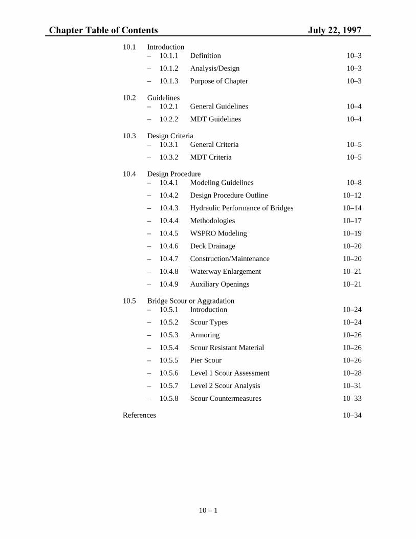
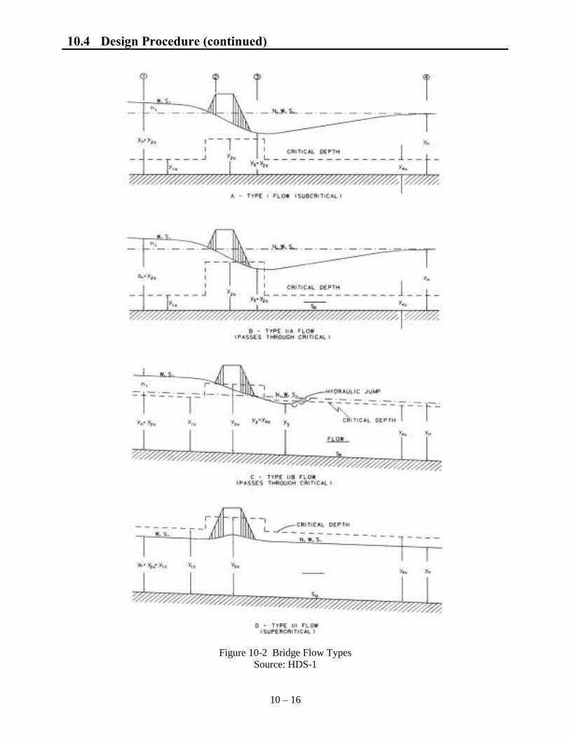
It is impractical to perform the hydraulic analysis for a bridge by manual calculations due to the interactive and complex nature of those computations. However, an example of the basic manual calculations is included in "Hydraulics of Bridge Waterways", HDS-1, FHWA. The hydraulic variables and flow types are defined in Figures 10-1 and 10-2 on the next two pages.
�� Backwater (h1) is measured relative to the normal water surface elevation without the effect of the bridge at the approach cross-section (Section 1). It is the result of contraction and re-expansion head losses and head losses due to bridge piers. Backwater can also be the result of a "choking condition" in which critical depth is forced to occur in the contracted opening with a resultant increase in depth and specific energy upstream of the contraction. This is illustrated in Figure 10-2.
�� Type I consists of subcritical flow throughout the approach, bridge, and exit cross sections and is the most common condition encountered in practice.

10.4 Design Procedure (continued)
10 – 15
Figure 10-1 Bridge Hydraulics Definition Sketch
Source: HDS-1
10.4 Design Procedure (continued)
10 – 16
Figure 10-2 Bridge Flow Types
Source: HDS-1

10.4 Design Procedure (continued)
10 – 17
Hydraulic Performance of Bridges (continued)
• Type IIA and IIB both represent subcritical approach flows which have been choked by the contraction resulting in the occurrence of critical depth in the bridge opening. In Type IIA the critical water surface elevation in the bridge opening is lower than the undisturbed normal water surface elevation. In the Type IIB it is higher than the normal water surface elevation and a weak hydraulic jump immediately downstream of the bridge contraction is possible.
• Type III flow is supercritical approach flow and remains supercritical through the bridge contraction. Such a flow condition is not subject to backwater unless it chokes and forces the occurrence of a hydraulic jump upstream of the contraction.
Methodologies 10.4.4
Momentum (HEC-2)
The Corps of Engineers HEC-2 model uses a variation of the momentum method in the special bridge routine when there are bridge piers. The momentum equation between cross-sections 1 and 3 is used to detect Type II flow and solve for the upstream depth in this case with critical depth in the bridge contraction. This model has been used for the majority of the flood insurance studies performed under the NFIP, and should generally be used to match results in FIS areas. However, it is recognized that the bridge analysis routines in HDS-1 and WSPRO may yield a better definition of actual hydraulic performance.
The HEC-RAS model is essentially an updated HEC-2 model. Although MDT has not used this model extensively, it is anticipated that is will be used where split flow is a consideration, such as in braided channels or near stream junctions. HEC-RAS has reportedly been modified to include the WSPRO bridge routines.
Energy (HDS-1)
The method developed by FHWA described in HDS-1 is an energy approach with the energy equation written between cross sections 1 and 4 as shown in Figure 10-1 for Type I flow. The backwater is defined in this case as the increase in the approach water surface elevation relative to the normal water surface elevation without the bridge.
This model utilizes a single typical cross section to represent the stream reach from points 1 to 4 on Figure 10-1. It also requires the use of a single energy gradient. This method is no longer recommended for final design analysis of bridges due to its inherent limitations but it may be useful for preliminary analysis and training. Studies performed by the Corps of Engineers for the FHWA show the need to utilize a multiple cross section method of analysis in order to achieve reasonable stage-discharge relationships at a bridge.

10.4 Design Procedure (continued)
10 – 18
Methodologies (continued)
Energy (WSPRO)
WSPRO combines step-backwater analysis with bridge backwater calculations. This method allows for pressure flow through the bridge, embankment overtopping, and flow through multiple openings and culverts. The bridge hydraulics still rely on the energy principle, but there is an improved technique for determining approach flow lengths and the introduction of an expansion loss coefficient. The flow-length improvement was found necessary when approach flows occur on very wide heavily-vegetated flood plains. The program also greatly facilitates the hydraulic analysis required to determine the least-cost alternative. The use of WSPRO is recommended for both preliminary and final analyses of bridge hydraulics. The output from this program facilitates scour computations.
Other Models
The USGS computer model E431 and the U.S. Soil Conservation Service computer model WSP-2 are recognized methods for computing water surface profiles, but should not be used for MDT projects without approval of MDT Hydraulics.
The BRI-STARS model is a quasi-two-dimensional program. The users manual indicates it incorporates the WSPRO model, and also includes the ability to model sediment transport, and resultant changes in the cross-sections. This model has not been used by MDT, but may be extensively used in the future.
2-Dimensional Modeling
The water surface profile and velocities in a section of river are often predicted using a computer model. In practice, most analysis is performed using one-dimensional methods such as the standard step method found in WSPRO. While one-dimensional methods are adequate for many applications, these methods cannot provide a detailed determination of the cross-stream water surface elevations, flow velocities or flow distribution.
Two-dimensional models are more complex and require more time to set up and calibrate. They require more field data than a one-dimensional model and more modeling time.
The USGS has developed a two-dimensional finite element model for the FHWA that is designated FESWMS. This model has been developed to analyze flow at bridge crossings where complicated hydraulic conditions exist. This two-dimensional modeling system is flexible and may be applied to many types of steady and unsteady flow problems including multiple opening bridge crossings, spur dikes, flood plain encroachments, multiple channels, flow around islands and flow in estuaries. Where the flow is essentially two-dimensional in the horizontal plane a one-dimensional analysis may lead to costly over-design or possibly improper design of hydraulic structures and improvements.

10.4 Design Procedure (continued)
10 – 19
Methodologies (continued)
Physical Modeling
Complex hydrodynamic situations defy accurate or practicable mathematical modeling. Physical models should be considered when:
• hydraulic performance data is needed that cannot be reliably obtained from mathematical modeling,
• risk of failure or excessive over-design is unacceptable, and
• research is needed.
The constraints on physical modeling are:
• size (scale),
• cost, and
• time.
WSPRO Modeling 10.4.5
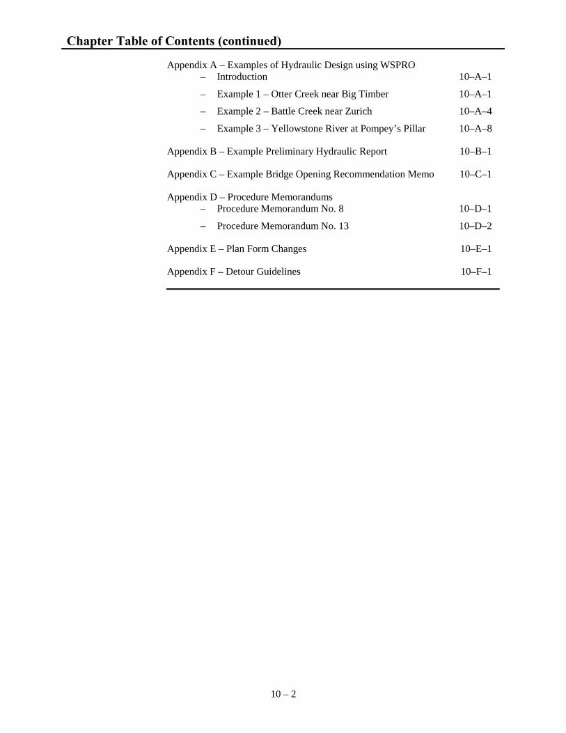
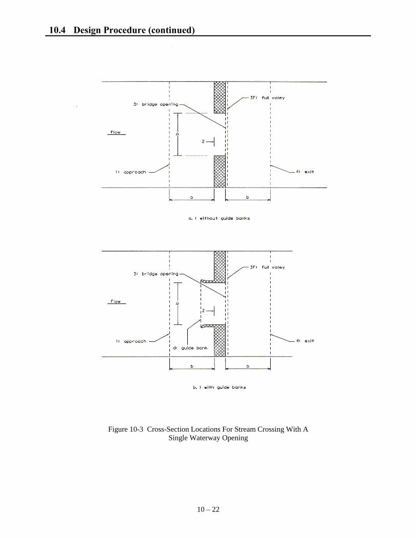
When using the WSPRO Model for MDT projects, the fixed-geometry mode should always be used. The design mode should not be used. The water surface profile used in the hydraulic analysis of a bridge should extend from a point downstream of the bridge that is beyond the influence of the constriction to a point upstream that is beyond the extent of the bridge backwater.The cross sections that are necessary for the energy analysis through the bridge opening for a single opening bridge without spur dikes are shown in Figure 10-3. The additional cross sections that are necessary for computing the entire profile are not shown in this figure. As a minimum, the model should start 1500' downstream, with additional sections as defined in Section 10.4.1. Cross sections 1, 3, and 4 are required for a Type I flow analysis and are referred to as the approach section, bridge section, and exit section, respectively. In addition, cross section 3F, which is called the full-valley section, is needed for the water surface profile computation without the presence of the bridge contraction. Cross section 2 is used as a control point in Type II flow but requires no input data. Two more cross sections must be defined if spur dikes and a roadway profile are specified.
Pressure flow through the bridge opening is assumed to occur when the depth just upstream of the bridge opening exceeds 1.1 times the hydraulic depth of the opening. The flow is then calculated as orifice flow with the discharge proportional to the square root of the effective head. Submerged orifice flow is treated similarly with the head redefined. WSPRO can also simultaneously consider embankment overflow as a weir discharge. This leads to flow classes 1 through 6 as given in the following table:

10.4 Design Procedure (continued)
10 – 20
WSPRO Modeling (continued)
Flow Classification According to Submergence Conditions (WSPRO User Instruction Manual - 1987)
Flow Through Bridge Opening Only
Class 1 - Free surface flow Class 2 - Orifice flow Class 3 - Submerged orifice flow
Flow Through Bridge Opening and Over Road Grade
Class 4 - Free surface flow Class 5 - Orifice flow Class 6 - Submerged orifice flow
In free-surface flow, there is no contact between the water surface and the low-girder elevation of the bridge. In orifice flow, only the upstream girder is submerged, while in submerged orifice flow both the upstream and downstream girders are submerged. A total of four different bridge types can be treated.
A user's instruction manual for WSPRO should serve as a source for more detailed information on using the computer model. Some examples of MDT projects are given in Appendix B with sample computer input and output data provided
Deck Drainage 10.4.6
Deck drainage is generally the responsibility of MDT's Bridge Bureau. The Hydraulics Section will provide assistance in special situations. Deck drainage needs should generally be computed using the Rational Formula.
Construction/ Maintenance 10.4.7
Construction plans should be reviewed by Hydraulics to note any changes in the stream from the conditions used in the design. When requested, a recommendation for detour structures will be provided. Guidelines are provided in Appendix F. The stream-crossing design shall incorporate measures which reduce maintenance costs whenever possible. These measures include spurs, guide banks, riprap protection of abutments and embankments, embankment overflow at lower elevations than the bridge deck, and alignment of piers with the flow.
Some Districts are reluctant to obtain permanent easements for certain hydraulic features (channel changes, riprap, drop structures, guide banks, etc.) which are located outside MDT Right-of-Way. It is therefore important to discuss these areas during plan-in-hand with the District. If the District elects to eliminate the use of permanent easements on the plans, Hydraulics will write a memo to the District describing the following:
• The intended function of the feature.
• The need for scheduled inspections (especially after flood events).
• The anticipated maintenance that will be required throughout the life of the feature
The District shall be requested to pass this information on to the entity responsible for maintenance (e.g., Counties in the case of Secondary Highways).

10.4 Design Procedure (continued)
10 – 21
Waterway Enlargement 10.4.8
There are situations where roadway and structural constraints dictate the vertical positioning of a bridge and result in a small vertical clearance between the low chord and the ground. Significant increases in span length provide small in-creases in effective waterway opening in these cases.
Excavating roadway fill that was previously placed in the channel can provide increased capacity. However, widening the channel for a short distance will have a minimal impact on the hydraulic capacity.
Auxiliary Openings 10.4.9
The need for auxiliary waterway openings, or relief openings as they are commonly termed, arises on streams with wide flood plains. The purpose of openings on the flood plain is to pass a portion of the flood flow in the flood plain when the stream reaches a certain stage. It does not provide relief for the principal waterway opening in the sense that an emergency spillway at a dam does, but has predictable capacity during flood events.
Basic objectives in choosing the location of auxiliary openings include:
• maintenance of flow distribution and flow patterns,
• accommodation of relatively large flow concentrations on the flood plain,
• avoidance of flood plain flow along the roadway embankment for long distances, and
• crossing of significant tributary or side channels.
• capacity to carry lower flows when the main crossing is subject to ice jams.
The technological weakness in modeling auxiliary openings is in the use of one-dimensional models to analyze two-dimensional flow. The development of 2-D models is a major step toward more adequate analysis of complex stream-crossing systems.
The most complex factor in designing auxiliary openings is determining the division of flow between the two or more structures. If incorrectly proportioned, one or more of the structures may be overtaxed during a flood event. The design of auxiliary openings should usually be generous to guard against that possibility.
MDT generally does not use auxiliary openings on the floodplain, because they provide only limited flow capacity.
10.4 Design Procedure (continued)
10 – 22
Figure 10-3 Cross-Section Locations For Stream Crossing With A Single Waterway Opening

10.4 Design Procedure (continued)
10 – 23
Figure 10-4 Cross-Section Locations In The Vicinity of Bridges

10.5 Bridge Scour or Aggradation
10 – 24
Introduction 10.5.1
Reasonable and prudent hydraulic analysis of a bridge design requires that an assessment be made of the proposed bridge's vulnerability to undermining due to potential scour. Because of the extreme hazard and economic hardships posed by a rapid bridge collapse, special considerations must be given to selecting appropriate flood magnitudes for use in the analysis. MDT typically evaluates scour at the design flow, the 100-year flow, and either the 500-year flow or the overtopping flow, whichever is smaller. At some locations, the greatest pier scour will occur at smaller flows, due to changes in the angle of attack. The hydraulic engineer must endeavor to always be aware of and use the most current scour forecasting technology.
The FHWA issued a Technical Advisory (TA 5140.20) on bridge scour in September 1988. The document "Interim Procedures for Evaluating Scour at Bridges" was an attachment to the Technical Advisory. The interim procedures were replaced by HEC-18 in 1991, which was revised in 1993 and again in 1995. Users of this manual should consult HEC-18 for a more thorough treatise on scour and scour prediction methodology. A companion FHWA document to HEC-18 is HEC-20, "Stream Stability at Highway Structures".
The following discussions represent MDT's current practices in regards to scour computations. These practices are subject to continuing change, as understanding of factors influencing scour improve.
Scour Types 10.5.2
Present technology dictates that bridge scour be evaluated as independent components:
• long term profile changes (aggradation/degradation),
• plan form change (lateral channel movement),
• contraction scour/deposition, and
• local scour (pier and abutment scour).
Long Term Profile Changes
Long term profile changes can result from stream bed profile changes that occur from aggradation and/or degradation.
• Aggradation is the deposition of bed load due to a decrease in the energy gradient. A braided channel is frequently an indication of aggradation.
• Degradation is the scouring of bed material due to increased stream sediment transport capacity which results from an increase in the energy gradient. A head cut is frequently an indication of degradation.
Forms of degradation and aggradation shall be considered as imposing a permanent future change for the stream bed elevation at a bridge site whenever they can be identified.

10.5 Bridge Scour or Aggradation (continued)
10 – 25
Scour Types (continued)
Plan Form Changes
The form and shape of the stream path created by its erosion and deposition characteristics comprise its morphology. A stream can be braided, straight, or meandering, or it can be in the process of changing from one form to another as a result of natural or manmade influences. An evaluation of the history of the stream morphology at a proposed stream-crossing site should be completed. The evaluation should include a review of the photo history and the flood history at the site. This evaluation should also include an assessment of any long-term trends in aggradation or degradation. Braided streams and alluvial fans shall especially be avoided for stream-crossing sites whenever possible.
Plan form changes are morphological changes such as meander migration or channel braiding. The lateral movement of meanders can threaten bridge approaches as well as increase scour by changing flow patterns approaching a bridge opening. A braided channel (often caused by an increase in sediment)can cause significant changes in the flow distribution and thus the bridge's flow contraction ratio. Recent braiding of a stream may indicate a change in upstream land use. The possibility of head cuts migrating upstream should not be overlooked. Some examples of plan form changes and the possible effects, taken from "Highways in the River Environment", are included in Appendix D.
Contraction
Channel contraction scour results from a constriction of the channel which may, in part, be caused by bridge piers in the waterway. Highways, bridges, and natural channel contractions are the most commonly encountered cause of contraction scour, also termed general scour.
Contraction scour should be computed using the equations described in HEC-18 (the average depth in the contracted section should be computed by dividing the cross-sectional area by the top width). It is necessary to determine whether the scour conditions are live-bed (moving bed material) or clear water. Computation of contraction scour is adapted from laboratory investigations of bridge contractions in non-armoring soils and, as such, must be used considering this qualification. The contraction scour equations in HEC-18 do not consider bed armoring, and therefore the computations yield values that are conservative in areas where armoring is a factor.
When the contraction scour equations yield values that appear to be unreasonably high (generally more than about 4 feet), it may be necessary to use a sediment routing model, such as BRI-STARS. This should be done only when the construction cost associated with the larger scour values significantly exceeds the cost of data collection and computation effort associated with the sediment routing model.

10.5 Bridge Scour or Aggradation (continued)
10 – 26
Armoring 10.5.3
Armoring occurs because a stream or river is unable, during a particular flood, to move the more coarse material comprising either the bed or, if some bed scour occurs, its underlying material. Armoring can be a tool to reduce the scour values in cobble streams. It may be necessary to do a material analysis of the stream bed, and apply shear stress equations to determine the impact of armoring. The possibility of armoring may also provide a false sense of security. If the channel is not currently armored, it is unlikely to become armored. Armoring can be considered when evaluating existing structures, using the methods described in HEC 20, but MDT does not generally use this technique for new bridges.
Armoring should be evaluated only when the cost of the additional foundation significantly exceeds the cost of the evaluation. Obtain bed material samples for all channel cross sections when armoring is to be evaluated. From these samples try to identify historical scour and associate it with a discharge. Also, determine the bed material size distribution and thickness in the bridge reach and from this distribution determine d16, d50, d84, and d90.
Scour Resistant Materials 10.5.4
Caution is necessary in determining the scour resistance of bed materials and the underlying strata. With sand size material, the passage of a single flood may result in the predicted scour depths. Conversely, in scour resistant material the maximum predicted depth of scour may not be realized during the passage of a particular flood; however, some scour resistant material may be lost. Commonly, this material is replaced with more easily scoured material. Thus, at some later date another (even smaller) flood may reach the predicted scour depth. Serious scour has been observed to occur in materials commonly perceived to be scour resistant such as consolidated soils and glacial till, as well as so-called bed rock streams and streams with gravel and boulder beds. Just because a bridge has survived a flood of some magnitude doesn�t mean it will survive the same flood again. If a bridge survived a large flood, and scour calculations indicate that it should not have survived, an attempt should be made to determine why the structure survived.
Pier Scour 10.5.5
The Colorado State University equation for pier scour has been used since the Technical Advisory was first issued. The factor K3 was added in the 1993 revision, and the factor K4 was added in the 1995 revision.
The procedure for estimating the width of the scour hole has also changed. The Technical Advisory recommended the estimated width of the bottom of the scour hole be 5 feet wider than the pier, and the angle of repose of the bed material was assumed to be 20° for a sand bed stream to get the side slope of the hole. The 1991 version of HEC-18 used the same bottom width, and an angle of repose of 30°. It also allowed a top width (on each side of the pier) equal to 2.75 times the scour depth. The 1993 revision of HEC-18 further revised these values to an estimated bottom width varying from zero to a width equal to the depth of scour, with the top width determined from an angle of repose varying between 30° and 44°, and a top width of 2.8 times the scour depth (again, on each side of the pier). The 1995 revision of HEC-18 provides the same general direction, but suggests a practical top width of 2.0 times the scour depth.

10.5 Bridge Scour or Aggradation (continued)
10 – 27
Pier Scour (continued)
Specific considerations when computing pier scour include:
• When computing total scour, the amount of pier scour is added to the amount of contraction scour, to determine the total scour at the pier.
• The skew angle between the pier and the flow direction. This angle may change at different water surface elevations. In some cases, more severe pier scour occurs at lower flows, because the flows are not lined up well with the piers. Review of flood photographs can be helpful in determining the appropriate angle.
• When the skew angle is severe, or changes dramatically at different flow rates, consideration should be given to using a single round pier. This
• type of pier does have a large hammerhead on top, which may negate some of the advantage of the round pier.
• When the top of the pier footing is above the contraction scour, the width of the footing needs to be considered in the scour analysis. A detailed description of this procedure is in HEC-18.
• In locations where debris is a consideration, and could be caught on the pier, the scour increases because the effective width of the pier increases. Computations of the impact of debris is indeterminate. In these situations, the support for the pier should be on rock or on piles. At one Montana location (St. Regis) where there was a pier scour failure, adding two feet to the pier width resulted in computed scour below the footing.
There are also several considerations in selecting the location for the piers, including:
• The spacing of the piers should be wider than the expected debris length.
• In locations where ice or debris are considerations, piers near the bank, on the outside of a bend, should be avoided.
• Where the channel has a thalweg that is well-defined, and appears to be unlikely to migrate substantially, the piers should be kept out of this area. One way to determine the long-term stability of the thalweg near existing structures is to compare the recent survey to the cross-section shown on the general layout for the existing bridge.

10.5 Bridge Scour or Aggradation (continued)
10 – 28
Level 1 Scour Assessment 10.5.6
A Level 1 scour assessment should be utilized to determine whether or not a Level 2 quantitative scour analysis is required for overlay or overlay and widen projects. The following guidelines are to be used to make a qualitative evaluation of the site. The USGS has completed a Level 1.5 analysis for all on-system bridges. This information should be reviewed to determine the need for additional analysis.
Full utilization of these guidelines will require a field review of the site. Prior to the field review, research of Hydraulic office files, stream gage information on historical flows, Bridge Maintenance files, flood studies, topographic maps, as-built plans, and aerial photographs shall be conducted. The following items shall be considered when evaluating potential scour.
Collect and summarize the following information as appropriate (see HEC-20 for a step-wise analysis procedure).
• Boring logs to define geologic substrata at the bridge site.
• Bed material size, gradation, and distribution in the bridge reach.
• Existing stream and floodplain cross section through the reach.
• Stream plan form.
• Watershed characteristics (e.g., land use).
• Scour data on other bridges in the area.
• Slope of energy grade line upstream and downstream of the bridge.
• History of flooding.
• Location of bridge site with respect to other bridges in the area, confluence with tributaries close to the site, bed rock controls (dams, old check structures, river training works, etc.), and confluence with another stream downstream.
• Character of the stream (perennial, flashy, intermittent, gradual peaks, etc.).
• Geomorphology of the site (floodplain stream; crossing of a delta; youthful, mature or old age stream; crossing of an alluvial fan; meandering, straight or braided stream; etc.).
• Erosion history of the stream.
• Development history (consider present and future conditions) of the stream and watershed. Collect maps, ground photographs, aerial photographs; interview local residents; check for water resource projects planned or contemplated
• Sand and gravel mining from the stream bed or floodplain up- and downstream from the site.
• Other factors that could affect the bridge.
• Make a qualitative evaluation of the site with an estimate of the potential for stream movement and its effect on the bridge.

10.5 Bridge Scour or Aggradation (continued)
10 – 29
Level 1 Scour Assessment (continued)
Abutment Scour
• Review site for existing abutment riprap protection and riprap keys and compare to As-Built drawings (there are a few structures out there that don�t have riprap keys).
• Look for poor stream alignment with regard to piers and abutments. Review angle of attack at "normal" and "flood" flows. There are documented cases of low flows causing a worst case scour scenario.
• Abutment scour tends to increase if the abutment is angled in an upstream direction.
• Vertical wall abutments will have twice the scour depths of spill-through abutments.
• Look for signs of significant overbank floodplain flows. Note that abutment scour will be most severe where the approach roadway embankment obstructs a significant amount of overbank flow.
• Look for countermeasures that may have been designed into the original project (spur dikes, jetties, training dikes, etc.) but may be missing or in a poor state of repair.
Pier Scour
• Look at location of piers in relation to the abutment. Could debris hang up on the pier and re-direct flows into the abutment or will debris tend to hang up more easily due to proximity of pier to the abutment?
• Look for piers on spread footings that are not keyed into bedrock. Are the footings visible or exposed?
• Note any visible pier tilting and deck or rail sagging. This could be an obvious sign of pier footings being undermined.
• Make a rough estimate of pier scour = 3 times pier width (see Fig. 4, HEC-18; Note: Fr=0.3) and compare to footing depth. It is also relatively simple to compute the pier scour from HEC-18 utilizing the hydraulic data on the bridge layout or previous bridge runs in the design file. If the likelihood of debris hang up is high, add additional width to pier when making pier scour computations. It is also easy to determine the pier width it would take to scour below the footing (for additional guidance, see Appendix G, HEC-18, November 1995).
• Be aware of lateral channel migration toward piers or bents located out of the active channel. Footings for these structures may have been constructed at higher elevations than those in the active channel.

10.5 Bridge Scour or Aggradation (continued)
10 – 30
Level 1 Scour Assessment (continued)
Contraction Scour
• Qualitatively speaking, live bed contraction scour increases if Q2>Q1 and W2<W1 (1-approach, 2-bridge).
• Is roadway overtopping possible or do all flood events have to pass through the bridge opening? Scour risk is more probable if no roadway relief is available.
• Bar formations downstream of a bridge may be an indicator of scour under the bridge.
General Comments
• Be aware of head cuts near bridge sites. Channel banks are a good indicator. Head cuts could point to rapid degradation.
• Watch structures below dams or lakes as these sites may have increased scour potential due to "hungry" water.
• Note that the presence of upstream structures (railroad, county road, etc.) in close proximity to the site in question may help to mitigate the affects of abutment and contraction scour at points downstream.
• Look for evidence of significant debris and ice which could promote additional scour at the site.
• Alluvial streams are more susceptible to stream instability.
• Bank appearance is a good indicator of channel stability.
• Relief bridges located in over banks may be subject to clear water scour.
Documentation
Upon completion of the office and field review of items noted above the designer shall document the findings in a scour report and indicate whether the structure is "scour critical" or at "low risk" for scour. This report and recommendations should be sent to the Bridge Bureau.
Should further recommendations be required one or more of the following actions may be taken. Note that engineering judgment must be utilized in applying the guidelines listed in this document.
1. Recommend additional core logs be taken to determine the competency of in-place material.
2. Recommend maintenance of "in-place" scour countermeasures or construction of "new" countermeasures such as riprap, guide banks, etc.
3. Recommend that the Bridge Bureau conduct a structural analysis to determine the affect of anticipated material loss due to scour. Use Figure 10-5 regarding calculated scour depth to determine when this action is required.
4. Request additional survey to determine extent of scour limits since original bridge construction.

10.5 Bridge Scour or Aggradation (continued)
10 – 31
Level 1 Scour Assessment (continued)
5. Request interdisciplinary team review (Bridge, Hydraulics, Geotechnical).
6. Recommend increased bridge inspection cycle.
7. Recommend underwater inspection.
8. Recommend increased maintenance with regard to drift removal from piers and abutments.
9. Recommend scour monitoring device.
10. Recommend Level 2 scour analysis and additional survey required to conduct such an analysis.
Level 2 Scour Analysis 10.5.7
A Level 2 scour analysis will be completed for every new bridge over a waterway. It may also be necessary for an existing bridge, depending on the results of the Level 1 or Level 1.5 analysis. Consideration should also be given to fixing the problem identified in the Level 1.5 analysis, rather than doing additional analysis. The information required for a Level 1 analysis should also be obtained for the Level 2 analysis. The Level 2 analysis is considered to be a conservative practice as it assumes that the scour components develop independently. The potential local scour to be calculated would be added to the contraction scour without considering the effects of contraction scour on the channel and bridge hydraulics. The general approach to a Level 2 scour analysis is as follows.
• Estimate the natural channel's hydraulics for a fixed bed condition based on existing conditions.
• Assess the expected profile and plan form changes.
• Adjust the fixed bed hydraulics to reflect any expected profile or plan form changes.
• Estimate contraction scour using the empirical contraction formula and the adjusted fixed bed hydraulics assuming no bed armoring.
• Estimate local scour using the adjusted fixed bed channel and bridge hydraulics assuming no bed armoring.
• Add the local scour to the contraction scour or aggradation to obtain the total scour.
• Determine the reference surface for measuring scour (see "Channel Scour at Bridges", FHWA-RD-95-184).
• Prepare a scour sketch, showing the channel cross-section at the bridge, the contraction scour and the local scour. An example scour sketch is shown in the Appendix.

10.5 Bridge Scour or Aggradation (continued)
10 – 32
Figure 10�5 Action Required for Calculated Scour Depths

10.5 Bridge Scour or Aggradation (continued)
10 – 33
Scour Countermeasures 10.5.8
Based on an assessment of potential scour provided by the Hydraulic Engineer, the structural designers can incorporate design features that will prevent or mitigate scour damage at piers. In general, circular piers or elongated piers with circular noses and an alignment parallel to the flow direction are a possible alternative. Spread footings (without pilings below) should be used only where the stream bed is extremely stable below the footing and where the top of the spread footing is founded at a depth below the maximum scour computed in Section 10.6.8. Drilled shafts or drilled piers are possible where pilings cannot be driven. Protection against general stream bed degradation can be provided by drop structures or grade-control structures in, or downstream of the bridge opening.
Rock riprap is often used, where stone of sufficient size is available, to armor abutment fill slopes and the area around the base of existing piers. HEC-18 makes the following statement about riprap at piers: "Riprap is not a permanent countermeasure for scour at piers for existing bridges and not to be used for new bridges." Riprap design information is presented in HEC-18.
Guide banks are recommended to align the approach flow with the bridge opening and to prevent scour around the abutments. Design guidance is provided in HEC-20.
The abutment scour equations tend to be very conservative. Use of riprap on the abutment, with the bottom of the key at or below the level of contraction scour, is generally considered to be an adequate countermeasure. The abutment riprap generally wraps around the abutment, and is kept within the right-of-way. Site conditions may require the riprap be extended upstream beyond the right-of-way, or a guide bank may need to be constructed. When a pier is close to the abutment, it may be prudent to extend the abutment riprap beyond the pier.
Other countermeasures which have use in certain situations include spurs, refusals, and windrow revetments. See HEC-18 for a detailed discussion on scour countermeasures.

References
10 – 34
AASHTO, Volume VII-Highway Drainage Guidelines, "Hydraulic Analyses for the Location and Design of Bridges", AASHTO Task Force on Hydrology and Hydraulics, 1982.
Bradley, J.N., "Hydraulics of Bridge Waterways," HDS-1, Federal Highway Administration, 1978. (Available from NTIS, 703/487-4600, publication PB86-181708/AS).
Corry, M.L., Jones, J.S., and Thompson, P.L., "The Design of Encroachments on Flood Plains Using Risk Analysis," Hydraulic Engineering Circular No. 17, Federal Highway Administration, Washington, D.C., 1980.
Federal Highway Administration, "Highways in the River Environment-Hydraulic and Environmental Design Considerations," Training and Design Manual, Federal Highway Administration, 1990.
Federal Highway Administration, "Federal Highway Program Manual," Vol. 6, Ch. 7, Sec. 3, Subsec. 2, November, 1979.
Shearman, J.O., "WSPRO User's Instructions," Draft Copy, U.S. Geological Survey, July, 1987.
U.S. Army Corps of Engineers, "HEC-2 Water Surface Profiles," User's Manual, September 1982.
U.S. Army Corps of Engineers, "Accuracy of Computed Water Surface Profiles," December, 1986.
Federal Highway Administration "Evaluating Scour at Bridges," HEC-18, 1995.
Kindsvater, C.E., "Discharge Characteristics of Embankment-Shaped Weirs," U.S. Geological Survey, WSP 1607-A, 1964.
Matthai, H.F., "Measurement of Peak Discharge at Width Contractions by Indirect Methods," U.S. Geological Survey, Techniques of Water Resources Investigations, Book 3, Ch. A4, 1967.
Schneider, V.R., Board, J.W., Colson, B.E., Lee, F.N., and Druffel, L., "Computation of Backwater and Discharge at Width Constriction of Heavily Vegetated Flood Plains," U.S. Geological Survey, WRI 76-129, 1977.
Federal Highway Administration, "Drainage at Highway Pavements," HEC-12, 1984.
U.S. Geological Survey, "Roughness Characteristics of Natural Channels," Water Supply Paper 1849, 1967.
National Institute of Water and Atmospheric Research Limited, "Roughness Characteristics of New Zealand Rivers," Kyle Street, PO Box 8602, Riccarton, Christchurch, New Zealand.
Federal Highway Administration, "Channel Scour at Bridges in the United States ," Publication No. FHWA-RD-95-184, 1996.
Federal Highway Administration "Stream Stability at Highway Structures," HEC-20, 1995.

Appendix A � Examples of Hydraulic Design of Bridges Using WSPRO
10 – A – 1
Introduction This appendix provides several examples of MDT projects designed using WSPRO. The only information provided is the input file and output table, along with a short narrative describing any unique features. Detailed information needed to use WSPRO is found in Reference 6. When using WSPRO with a large number of data points, it is important to review the complete output carefully (not just the summary output). Some situations limit the maximum number of cross-section data points to about 45. The examples include user defined tables, which are variable depending on the designer�s preference.
Example 1 Otter Creek near Big Timber
In this example, the roadway overtops in a very wide area, and the low beam of the existing bridge is about 1.4 meters above the low point in the roadway (this project was done completely in the metric system). Therefore, this model used the composite section approach at the bridge. The composite section included the channel under the bridge, along with the roadway profile. The impacts of the bridge superstructure are ignored in this situation. Another unique aspect of this project is the distance downstream that the profile started. Due to the presence of a control section, determined prior to the survey request, the first cross-section was 755 meters downstream (rather than the normal 450 meters downstream). This helped insure convergence of the water surface profiles downstream from the bridge. Finally, some of the cross-sections downstream from the bridge were modified. Based on review of the site, it was determined that the overbank areas immediately downstream from the bridge were ineffective in carrying flows, so the cross-sections were not extended into these overbank areas. This project illustrates the use of the HP command and the resultant velocity distribution.
T1 Otter Creek BR 478-1(3)2 T2 Northeast of Big Timber T3 New Bridge 4 Meter Bottom @ 1222 * All Distances and Elevations in Meters * SI 1 UT 8 5 7 2 12 26 1 28 25 42 41 Q 16 SK .0028 * 755 Meters Down Stream XS 755 0 GR -48,1224.75 -45,1224.72 -42,1224.66 -39,1224.54 GR -36,1224.41 -33,1223.81 -30,1223.43 -27,1222.80 GR -24,1222.25 -21,1221.68 -18,1221.12 -15,1220.95 GR -12,1220.82 -9.1,1220.62 -6.1,1220.54 -4.8,1220.04 GR 0,1219.84 3.7,1220.14 6.5,1220.94 8.6,1221.85 GR 10.6,1222.11 12.6,1222.40 14.5,1222.83 17.5,1223.76 GR 20.5,1224.36 23.5,1224.75 26,1225.27 N 0.060 0.030 0.060 SA -18 8.6 XS 625 130 GR -16,1223.41 -13.6,1222.71 -10.6,1221.93 -7.6,1221.33 GR -4.9,1220.68 -4.1,1220.06 -4.0,1219.96 -1.7,1219.56 GR 0,1219.69 3.3,1220.01 4,1220.73 7,1220.87

Appendix A � Examples of Hydraulic Design of Bridges Using WSPRO (cont.)
10 – A – 2
GR 10,1220.79 13,1220.81 16,1220.79 30,1220.81 SA -4.9 4 XS 330 425 GR -52,1225.48 -41,1223.93 -35,1223.49 -32,1223.27
Example 1 (continued)
GR -29,1223.17 -26,1222.94 -25,1222.92 -23,1222.68 GR -20,1222.07 -17,1222.03 -14.2,1222.12 -11.2,1221.95 GR -8.2,1221.87 -5.2,1221.78 -4.2,1221.05 -1.7,1220.88 GR 0,1220.55 2.2,1220.40 3.4,1220.26 3.4,1221.01 GR 4,1221.88 7,1222.02 8.4,1222.23 9.4,1222.63 GR 12.4,1222.99 13.6,1223.18 16.6,1223.79 SA -5.2 4 XS 135 620 GR -12,1225.38 -10.7,1224.97 -7.7,1223.78 -4.7,1222.61 GR -3.6,1221.97 -1.8,1221.52 0,1221.57 3.3,1221.92 GR 4.1,1222.58 9,1222.71 10,1222.84 13,1222.81 GR 15.5,1222.90 18.5,1223.01 20.5,1222.99 SA -4.7 4.1 XS 20 735 GR -22.8,1225.36 -20.1,1224.99 -17.1,1224.71 -13.6,1224.60 GR -10.6,1224.35 -7.6,1224.18 -6.4,1223.80 -3.8,1222.79 GR -2.1,1222.11 0,1221.38 2.1,1222.16 3.6,1223.48 GR 6.6,1223.87 9.6,1223.91 12.6,1223.72 15.6,1223.71 GR 18.6,1223.94 20.6,1223.84 SA -6.4 6.6 * New Bridge 4 Meter Bottom @ 1222 XS BRD 752 GR -68.7,1230.33 GR -10.5,1226.1 -2.3,1222.0 0,1221.89 GR 1.7,1222.0 7.7,1225.0 GR 12.7,1226.14 36.2,1225.02 GR 77.2,1224.12 107.3,1223.83 182.3,1224.04 227.3,1224.37 GR 242,1224.70 259.3,1225.31 317.3,1228.99 446,1233.12 SA -6.3 5.7 HP 2 BRD 1223.31 0 1223.31 16 XS BR2 758 GR -68.7,1230.33 GR -10.5,1226.1 -2.3,1222.0 0,1221.89 GR 1.7,1222.0 7.7,1225.0 GR 12.7,1226.14 36.2,1225.02 GR 77.2,1224.12 107.3,1223.83 182.3,1224.04 227.3,1224.37 GR 242,1224.70 259.3,1225.31 317.3,1228.99 446,1233.12 SA -6.3 5.7 XS 20U 775 GR -8.5,1225.32 -6.7,1224.03 -5.2,1223.57 -3.7,1222.71 GR -3.3,1222.26 0,1221.98 3.5,1222.27 5,1223.05 GR 8,1223.63 11,1223.99 14,1224.02 17,1224.09 GR 20,1224.21 43.5,1224.45 77.2,1224.17 107.3,1223.68 SA -5.2 5 EX ER

Appendix A � Examples of Hydraulic Design of Bridges Using WSPRO (cont.)
10 – A – 3
= = = User Defined Table 1 of 1 = = = Example 1
(continued) SRD WSEL Q AREA YMIN VEL K
1 755 .000 1220.978 16.000 13.0 1219.840 1.230 302. 2 625 130.000 1221.202 16.000 22.8 1219.560 .702 553. 3 330 425.000 1221.698 16.000 8.4 1220.260 1.911 243. 4 135 620.000 1222.652 16.000 7.4 1221.520 2.149 210. 5 20 735.000 1223.236 16.000 8.5 1221.380 1.890 268. 6 BRD 752.000 1223.313 16.000 8.9 1221.890 1.791 278. 7 BR2 758.000 1223.341 16.000 9.2 1221.890 1.741 289. 8 20U 775.000 1223.427 16.000 11.2 1221.980 1.425 370.
CRWS EGL XSTW XSWP 1 755 1220.675 1221.055 22.097 22.337 2 625 1220.554 1221.254 37.068 37.747 3 330 1221.435 1221.884 8.983 10.300 4 135 1222.502 1222.894 11.645 12.138 5 20 1222.862 1223.418 8.273 9.157 6 BRD 1222.954 1223.477 9.255 9.882 7 BR2 1222.954 1223.496 9.366 10.006 8 20U 1222.933 1223.536 11.904 12.548 New Bridge 4 Meter Bottom @ 1222 *** Beginning Velocity Distribution For Header Record BRD ***
SRD Location: 752.000 Header Record Number 6
Water Surface Elevation: 1223.310 Element # 1 Flow: 16.000 Velocity: 1.80 Hydraulic Depth: .962
Cross-Section Area: 8.89 Conveyance: 276.58 Bank Stations -> Left: -4.920 Right: 4.320
X Sta. –4.9 –3.1 –2.6 –2.2 –1.9 –1.6 A(I) .8 .5 .5 .4 .4 V(I) 1.00 1.49 1.77 1.89 2.04 D(I) .45 1.03 1.25 1.32 1.34 X Sta. –1.6 –1.3 –1.1 –.8 –.5 –.3 A(I) .4 .4 .4 .4 .4 V(I) 2.09 2.15 2.15 2.23 2.22 D(I) 1.35 1.36 1.38 1.39 1.40 X Sta. –.3 .0 .2 .5 .8 1.0 A(I) .4 .4 .4 .4 .4 V(I) 2.23 2.23 2.16 2.16 2.11 D(I) 1.41 1.41 1.4 1.38 1.36
Appendix A � Examples of Hydraulic Design of Bridges Using WSPRO (cont.)
10 – A – 4
X Sta. 1.0 1.3 1.6 2.0 2.5 4.3
A(I) .4 .4 .5 .5 .8 V(I) 2.06 1.91 1.75 1.51 .99 D(I) 1.34 1.32 1.25 1.03 .45 ER
Example 1 (continued)
= = = Normal End of WSPRO Execution = = = = = = Elapsed Time: 0 Minutes, 2 Seconds = = =
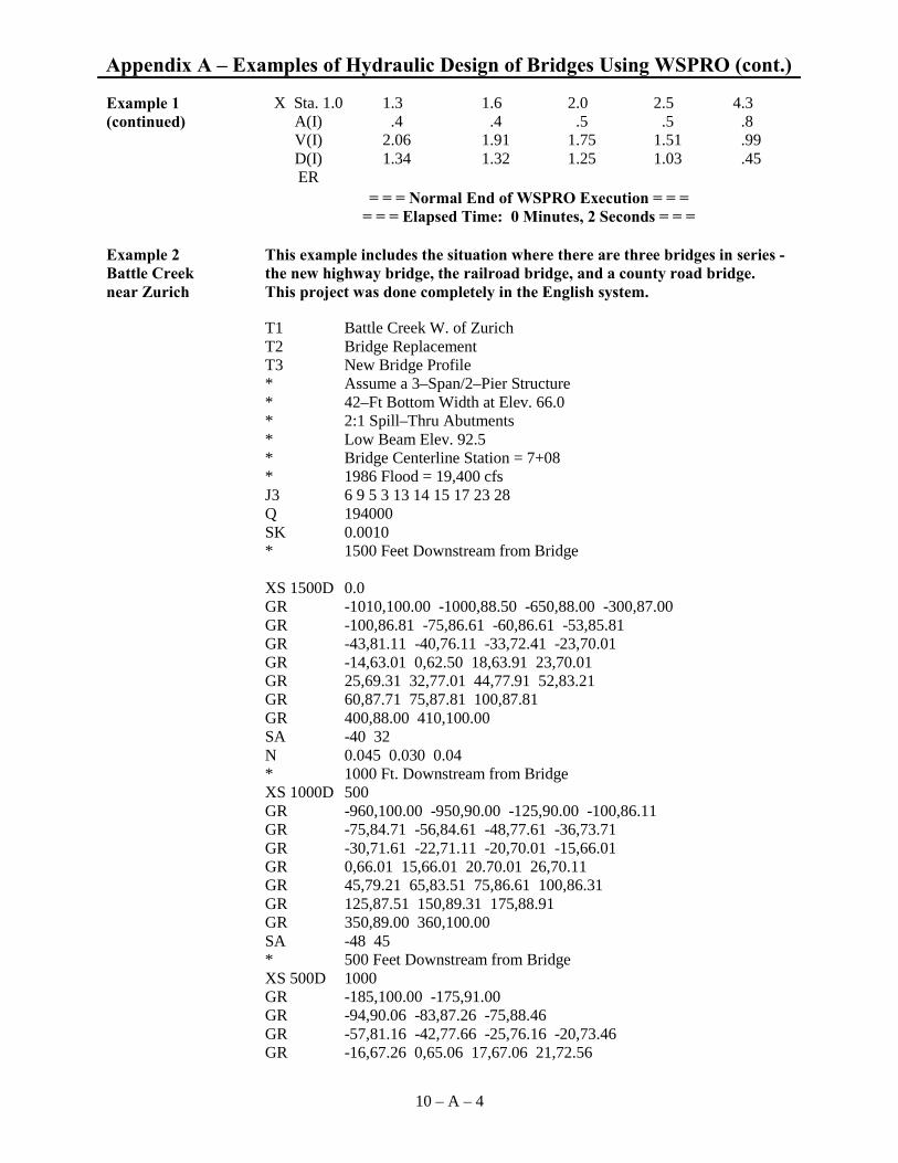
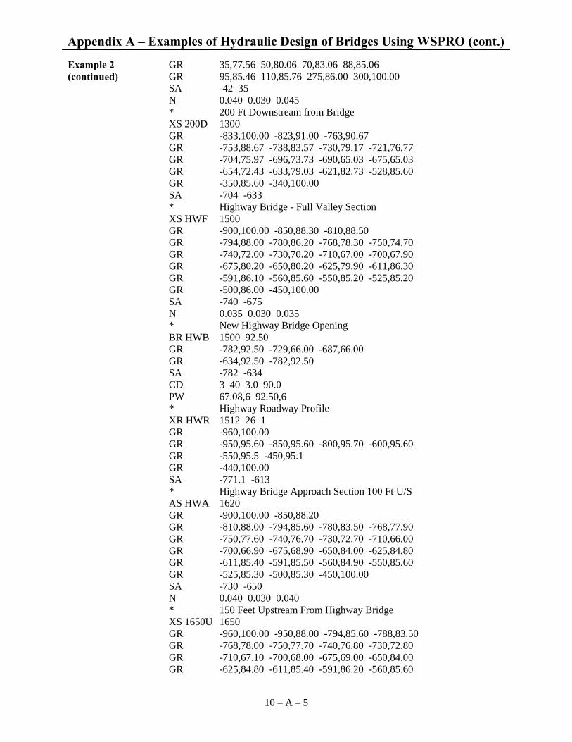
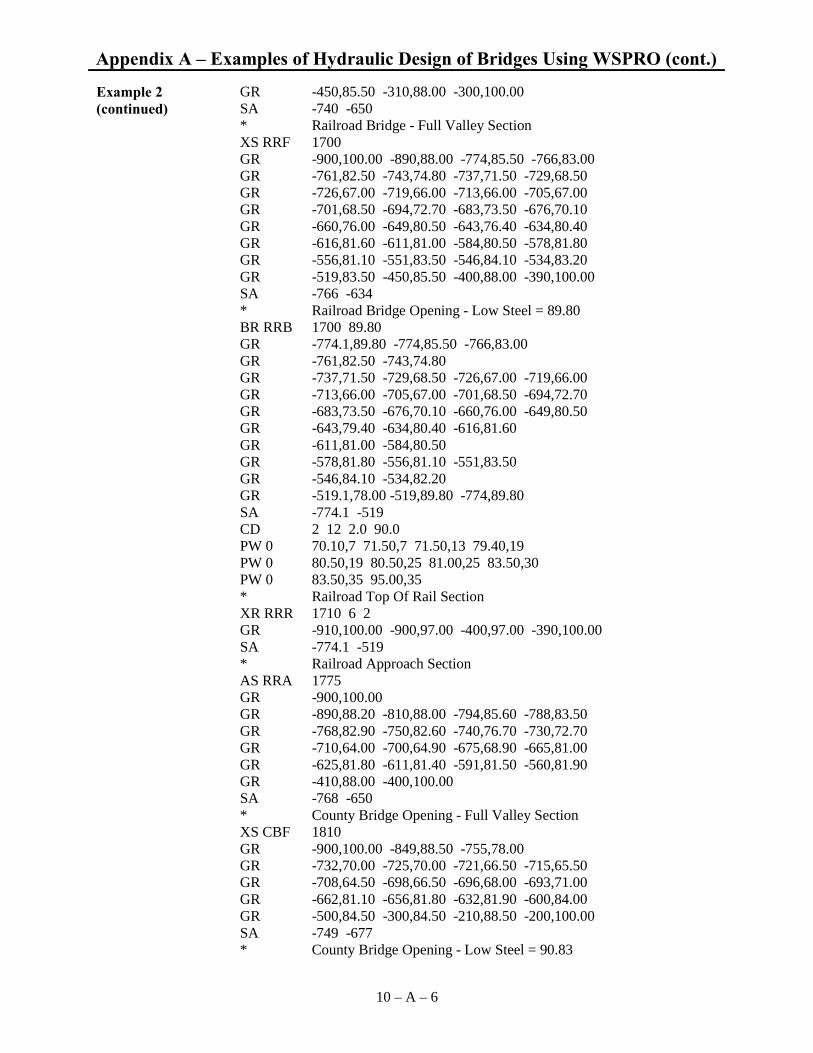
Example 2 Battle Creek near Zurich
This example includes the situation where there are three bridges in series - the new highway bridge, the railroad bridge, and a county road bridge. This project was done completely in the English system.
T1 Battle Creek W. of Zurich T2 Bridge Replacement T3 New Bridge Profile * Assume a 3–Span/2–Pier Structure * 42–Ft Bottom Width at Elev. 66.0 * 2:1 Spill–Thru Abutments * Low Beam Elev. 92.5 * Bridge Centerline Station = 7+08 * 1986 Flood = 19,400 cfs J3 6 9 5 3 13 14 15 17 23 28 Q 194000 SK 0.0010 * 1500 Feet Downstream from Bridge XS 1500D 0.0 GR -1010,100.00 -1000,88.50 -650,88.00 -300,87.00 GR -100,86.81 -75,86.61 -60,86.61 -53,85.81 GR -43,81.11 -40,76.11 -33,72.41 -23,70.01 GR -14,63.01 0,62.50 18,63.91 23,70.01 GR 25,69.31 32,77.01 44,77.91 52,83.21 GR 60,87.71 75,87.81 100,87.81 GR 400,88.00 410,100.00 SA -40 32 N 0.045 0.030 0.04 * 1000 Ft. Downstream from Bridge XS 1000D 500 GR -960,100.00 -950,90.00 -125,90.00 -100,86.11 GR -75,84.71 -56,84.61 -48,77.61 -36,73.71 GR -30,71.61 -22,71.11 -20,70.01 -15,66.01 GR 0,66.01 15,66.01 20.70.01 26,70.11 GR 45,79.21 65,83.51 75,86.61 100,86.31 GR 125,87.51 150,89.31 175,88.91 GR 350,89.00 360,100.00 SA -48 45 * 500 Feet Downstream from Bridge XS 500D 1000 GR -185,100.00 -175,91.00 GR -94,90.06 -83,87.26 -75,88.46 GR -57,81.16 -42,77.66 -25,76.16 -20,73.46 GR -16,67.26 0,65.06 17,67.06 21,72.56
Appendix A � Examples of Hydraulic Design of Bridges Using WSPRO (cont.)
10 – A – 5
GR 35,77.56 50,80.06 70,83.06 88,85.06 Example 2 (continued) GR 95,85.46 110,85.76 275,86.00 300,100.00 SA -42 35 N 0.040 0.030 0.045 * 200 Ft Downstream from Bridge XS 200D 1300 GR -833,100.00 -823,91.00 -763,90.67 GR -753,88.67 -738,83.57 -730,79.17 -721,76.77 GR -704,75.97 -696,73.73 -690,65.03 -675,65.03 GR -654,72.43 -633,79.03 -621,82.73 -528,85.60 GR -350,85.60 -340,100.00 SA -704 -633 * Highway Bridge - Full Valley Section XS HWF 1500 GR -900,100.00 -850,88.30 -810,88.50 GR -794,88.00 -780,86.20 -768,78.30 -750,74.70 GR -740,72.00 -730,70.20 -710,67.00 -700,67.90 GR -675,80.20 -650,80.20 -625,79.90 -611,86.30 GR -591,86.10 -560,85.60 -550,85.20 -525,85.20 GR -500,86.00 -450,100.00 SA -740 -675 N 0.035 0.030 0.035 * New Highway Bridge Opening BR HWB 1500 92.50 GR -782,92.50 -729,66.00 -687,66.00 GR -634,92.50 -782,92.50 SA -782 -634 CD 3 40 3.0 90.0 PW 67.08,6 92.50,6 * Highway Roadway Profile XR HWR 1512 26 1 GR -960,100.00 GR -950,95.60 -850,95.60 -800,95.70 -600,95.60 GR -550,95.5 -450,95.1 GR -440,100.00 SA -771.1 -613 * Highway Bridge Approach Section 100 Ft U/S AS HWA 1620 GR -900,100.00 -850,88.20 GR -810,88.00 -794,85.60 -780,83.50 -768,77.90 GR -750,77.60 -740,76.70 -730,72.70 -710,66.00 GR -700,66.90 -675,68.90 -650,84.00 -625,84.80 GR -611,85.40 -591,85.50 -560,84.90 -550,85.60 GR -525,85.30 -500,85.30 -450,100.00 SA -730 -650 N 0.040 0.030 0.040 * 150 Feet Upstream From Highway Bridge XS 1650U 1650 GR -960,100.00 -950,88.00 -794,85.60 -788,83.50 GR -768,78.00 -750,77.70 -740,76.80 -730,72.80 GR -710,67.10 -700,68.00 -675,69.00 -650,84.00 GR -625,84.80 -611,85.40 -591,86.20 -560,85.60
Appendix A � Examples of Hydraulic Design of Bridges Using WSPRO (cont.)
10 – A – 6
GR -450,85.50 -310,88.00 -300,100.00 Example 2 (continued) SA -740 -650 * Railroad Bridge - Full Valley Section XS RRF 1700 GR -900,100.00 -890,88.00 -774,85.50 -766,83.00 GR -761,82.50 -743,74.80 -737,71.50 -729,68.50 GR -726,67.00 -719,66.00 -713,66.00 -705,67.00 GR -701,68.50 -694,72.70 -683,73.50 -676,70.10 GR -660,76.00 -649,80.50 -643,76.40 -634,80.40 GR -616,81.60 -611,81.00 -584,80.50 -578,81.80 GR -556,81.10 -551,83.50 -546,84.10 -534,83.20 GR -519,83.50 -450,85.50 -400,88.00 -390,100.00 SA -766 -634 * Railroad Bridge Opening - Low Steel = 89.80 BR RRB 1700 89.80 GR -774.1,89.80 -774,85.50 -766,83.00 GR -761,82.50 -743,74.80 GR -737,71.50 -729,68.50 -726,67.00 -719,66.00 GR -713,66.00 -705,67.00 -701,68.50 -694,72.70 GR -683,73.50 -676,70.10 -660,76.00 -649,80.50 GR -643,79.40 -634,80.40 -616,81.60 GR -611,81.00 -584,80.50 GR -578,81.80 -556,81.10 -551,83.50 GR -546,84.10 -534,82.20 GR -519.1,78.00 -519,89.80 -774,89.80 SA -774.1 -519 CD 2 12 2.0 90.0 PW 0 70.10,7 71.50,7 71.50,13 79.40,19 PW 0 80.50,19 80.50,25 81.00,25 83.50,30 PW 0 83.50,35 95.00,35 * Railroad Top Of Rail Section XR RRR 1710 6 2 GR -910,100.00 -900,97.00 -400,97.00 -390,100.00 SA -774.1 -519 * Railroad Approach Section AS RRA 1775 GR -900,100.00 GR -890,88.20 -810,88.00 -794,85.60 -788,83.50 GR -768,82.90 -750,82.60 -740,76.70 -730,72.70 GR -710,64.00 -700,64.90 -675,68.90 -665,81.00 GR -625,81.80 -611,81.40 -591,81.50 -560,81.90 GR -410,88.00 -400,100.00 SA -768 -650 * County Bridge Opening - Full Valley Section XS CBF 1810 GR -900,100.00 -849,88.50 -755,78.00 GR -732,70.00 -725,70.00 -721,66.50 -715,65.50 GR -708,64.50 -698,66.50 -696,68.00 -693,71.00 GR -662,81.10 -656,81.80 -632,81.90 -600,84.00 GR -500,84.50 -300,84.50 -210,88.50 -200,100.00 SA -749 -677 * County Bridge Opening - Low Steel = 90.83

Appendix A � Examples of Hydraulic Design of Bridges Using WSPRO (cont.)
10 – A – 7
BR CBB 1810 90.83 Example 2 (continued) GR -749.1,90.83 -749,78.00 GR -732,70.00 -725,70.00 -721,66.50 -715,65.50 GR -708,64.50 -698,66.50 -696,68.00 -693,71.00 GR -677,81.10 -666,81.80 -652.1,83.90 -652,90.83 GR -749.1,90.83 SA -749.1 -652 CD 2 20 2.0 90.0 * County Bridge Roadway Profile XR CBR 1820 20 2 2.0 GR -760,100.00 -750,93.00 -650,93.00 -550,90.00 GR 750,90.00 760,100.00 SA -749.1 -652 * County Bridge Approach Section AS CBA 2000 GR -110,100.00 -100,89.51 -75,89.51 -70,88.51 GR -60,79.61 -40,76.51 -32,73.21 -17,72.81 GR -14,68.41 0,67.11 15,68.81 18,74.61 GR 27,77.81 43,85.61 650,86.41 660,100.00 SA -60 43 * 1000 Ft Upstream From Bridge XS 1000U 2500 GR -160,100.00 -150,90.40 -125,90.33 -108,90.33 GR -26,79.23 -22,73.83 -17,68.23 GR 0,66.23 17,66.33 20,73.93 45,74.13 55,76.93 GR 73,79.33 80,86.63 100,86.63 125,86.63 GR 400,86.63 410,100.00 SA -26 73 * 1500 Ft Upstream From Bridge XS 1500U 3000 GR -135,100.00 -125,91.29 -100,91.29 -80,91.09 GR -65,90.89 -60,87.69 -45,78.19 -30,75.29 GR -18,74.49 -11,72.19 -10,68.89 0,66.89 GR 10,67.39 14,76.29 35,76.99 40,81.69 GR 65,86.19 70,88.39 100,88.49 125,87.79 GR 400,87.79 410,100.00 SA -45 40 EX ER FIRST USER DEFINED TABLE XSID:CODE SRD FLEN Q WSEL VEL FR# CRWS AREA 1500D:XS 0 **** 19400 88.71 6.08 1.23 80.53 3193 1000D:XS 500 500 19400 89.38 7.78 .76 **** 2493 500D:XS 1000 500 19400 90.15 6.40 .55 **** 3032 200D:XS 1300 300 19400 90.71 5.43 .46 **** 3575 HWF:FV 1500 200 19400 90.89 5.85 .45 **** 3317 HWB:BR 1500 200 19400 90.39 8.76 .44 81.53 2214 HWR:RG 1512 **** 0 **** 1.00 **** **** **** HWS:AS 1620 86 19400 91.22 5.41 .41 82.67 3588 1650U:XS 1650 30 19400 91.57 3.81 .34 **** 5093 RRF:FV 1700 50 19400 91.65 3.97 .28 **** 4881

Appendix A � Examples of Hydraulic Design of Bridges Using WSPRO (cont.)
10 – A – 8
RRB:BR 1700 **** 19141 89.80 7.08 .38 83.52 2705Example 2 (continued) RRR:RG 1710 **** 0 **** 2.00 **** **** **** RRA:AS 1775 68 19400 92.56 3.83 .26 83.88 5070 1785U:XS 1785 10 19400 92.65 3.11 .24 **** 6235 CBF:FV 1810 25 19400 92.67 2.96 .22 **** 6548 CBB:BR 1810 **** 5226 90.83 3.13 .13 75.20 1668 CBR:RG 1820 170 14170 92.62 2.00 **** **** **** CBA:AS 2000 707 19400 92.93 3.06 .25 84.48 6343 1000U:XS 2500 500 19400 92.98 3.91 .31 **** 4956 1500U:XS 3000 500 19400 93.04 4.99 .45 **** 3889 YMIN XSTW 62.50 1401 66.01 471 65.06 384 65.03 424 67.00 379 66.00 140 95.10 **** 66.00 383 67.10 646 66.00 383 97.00 **** 64.00 487 64.10 689 64.50 661 64.50 0 90.00 **** 67.11 758 66.23 557 66.89 531 Example 3 Yellowstone River at Pompey�s Pillar
In this example of modeling the existing bridge, flood photographs were used to calibrate the model. Photographs of the May 1978 flood were used, along with gaging station records on the Yellowstone River at Billings and on Pryor Creek near Billings. The gaging station records were used to estimate the flow, and the photographs were used to estimate the water surface elevation. Water was over the road at a sag in the north approach, so the width of the water surface was directly related to a known water surface elevation. This example also shows the use of the PD command to describe piers. This project was also completed entirely in the metric system.
T1 Yellowstone River BR 568-1(8)2 T2 At Pompeys Pillar T3 Existing Bridge May 1978 Flow * All Distances And Elevations In Meters * Q25=1900 M3/S, Q100=2220 M3/S, Q500=2580 M3/S SI 1 UT 8, 7, 5, 12, 26, 25, 28, 2, 42, 41 Q 1775 SK .0018

Appendix A � Examples of Hydraulic Design of Bridges Using WSPRO (cont.)
10 – A – 9
* 470 Meters Downstream Example 3 (continued) XS 470D -470 GR -56,887 -28,881 GR 0,874.99 3,874.32 10,873.55 17.2,873.43 GR 34.9,873.13 53.4,874.11 75.4,874.36 92.6,874.39 GR 104.9,874.72 114.2,875.00 145.8,875.73 164.5,876.51 GR 300,878 N 0.050 0.032 0.050 SA 0 164.5 * 260 Meters Downstream XS 260D -260 GR -185,886 -110,879.3 -90,876.5 -80,876.5 GR -60,878.7 -10,877.5 GR 0,875.63 4.6,874.98 25.3,874.63 GR 44.2,874.21 68.9,874.14 91.5,874.37 118.5,874.45 GR 136.5,875.03 143.8,875.62 149.8,878.08 GR 300,878.2 SA 0 143.8 * 150 Meters Downstream XS 150D -150 GR -375,886 -300,879.3 -230,878.9 -220,876.5 GR -210,876.5 -190,878.7 -10,877.5 GR 0,875.69 4.6,874.67 14.3,874.73 GR 27.1,874.84 40.1,874.17 54,873.85 72.9,873.80 GR 96.1,874.32 110.9,874.73 128.4,875.01 133.5,875.71 GR 137.2,878.29 GR 300,878.5 SA 0 133.5 * 84 Meters Downstream XS Exit -84 GR 0,888.49 9.5,886.27 42,883.55 62.4,881.81 GR 72.2,880.06 83.1,879.23 151.4,878.32 157.6,876.61 GR 162.4,876.54 168,877.65 182.5,877.50 191,878.06 GR 207.6,878.03 237.4,878.26 257.9,877.93 263.4,878.23 GR 316.2,877.01 GR 361.1,878.12 391.1,875.37 392.7,875.07 398.1,874.69 GR 406.6,874.75 416.3,875.07 425.8,875.29 432.7,875.13 GR 436.7,874.62 437.9,874.47 446.8,873.91 458.6,873.48 GR 466.9,873.30 476.4,873.33 493.1,874.64 495.6,874.85 GR 506.1,875.30 510.7,874.98 513,874.79 516.7,875.10 GR 517.9,875.42 524.3,878.40 573.8,879.33 578.2,878.59 GR 614.5,877.89 631.1,877.84 661.5,877.84 692.5,877.70 SA 392.7 524.3 XS FullV -3 GR 0,881.98 34.2,880.60 60.4,879.60 94.3,878.58 GR 140.8,877.57 162.2,877.85 176.6,877.74 204.6,878.38 GR 226.6,878.17 242.6,878.28 262.8,878.62 281.9,876.73 GR 315.2,875.91 339.7,878.37 357.3,876.74 363.0,875.45 GR 368.9,875.09 386.2,875.08 396.3,875.10 407.4,875.29 GR 413.3,874.67 418.4,874.66 428.1,874.21 436.0,873.11 GR 441.5,871.57 GR 470,872 482.9,875.62 491.5,878.44 509.7,878.20

Appendix A � Examples of Hydraulic Design of Bridges Using WSPRO (cont.)
10 – A – 10
GR 539.2,878.22 Example 3 SA 339.7 491.5
* Existing Bridge BR Brdge -3 881 GR 285.4,881 285.4,876.73 GR 315.2,875.91 339.7,878.37 357.3,876.74 363.0,875.45 GR 368.9,875.09 386.2,875.08 396.3,875.10 407.4,875.29 GR 413.3,874.67 418.4,874.66 428.1,874.21 436.0,873.11 GR 441.5,871.57 GR 470,872 482.9,875.62 482.9,881 285.4,881 CD 2 6 2 882 PD 0 871,2,1 874.7,2,1 874.7,4,2 876.6,4,4 876.6,8,4 N 0.05 0.032 0.05 SA 339.7 482.9 XR Road -3 24 GR -19.4,882.09 27.5,880.46 72,879.35 135.2,878.70 GR 155.4,878.69 180.9,878.77 203.4,878.90 224.2,879.13 GR 284.2,882.07 285.4,882.14 482.9,882.15 484.3,882.07 GR 511.3,880.04 530.9,879.33 552.4,879.11 578,879.15 GR 595.3,879.15 610.6,879.12 626.5,879.12 642.2,879.16 GR 663.4,879.28 698.6,879.34 700.4,879.37 755,879.35 GR 791.2,879.37 803.6,879.40 838.2,879.33 852,879.27 GR 883.6,879.43 947.5,879.42 * 125 Meters Upstream XS Appr 125 GR 330,882 343,877.06 GR 365.8,876.57 385.7,876.64 411.1,875.47 415.5,875.16 GR 419,874.85 423.1,874.47 430,874.19 440.2,874.01 GR 454,873.86 471,873.87 483.3,874.23 496.2,874.07 GR 506.9,874.40 515.3,875.13 543.7,877.10 548.1,875.41 GR 548.4,875.23 549.3,875.33 573.1,877.64 574.4,878.59 GR 575.5,878.66 585.7,878.54 588.7,879.16 593,879.16 GR 596.7,878.98 599,878.43 600,878.39 SA 385.7 543.7 * 240 Meters Upstream XS 240U 240 GR 246,882.05 253.3,882.16 300.4,878.48 338.6,874.52 GR 344.3,874.08 351.4,873.57 365.8,873.05 377.4,872.65 GR 391.3,872.56 401,873.57 408.3,874.35 418.3,875.03 GR 469.9,877.41 471.1,878.72 498.6,878.92 539.7,878.71 GR 559.8,878.68 613.3,877.94 625.8,876.96 GR 627.1,877.43 627.9,877.43 639.8,877.94 683.9,878.65 SA 253.3 471.1 EX ER

Appendix A � Examples of Hydraulic Design of Bridges Using WSPRO (cont.)
10 – A – 11
=== User Defined Table 1 of 1 === Example 3 SRD Q WSEL YMIN VEL EGL CRWS
1 470D -470.000 1775.000 877.946 873.129 2.625 878.386 876.836 2 260D -260.000 1775.000 878.293 874.139 2.736 878.780 877.042 3 150D -149.999 1775.000 878.491 873.799 2.524 878.959 877.083 4 Exit -83.999 1775.000 878.693 873.299 1.969 879.049 877.172 5 FullV -3.000 1775.000 878.862 871.569 1.845 879.134 876.806 6 Appr 124.999 1775.000 878.973 873.859 2.129 879.257 877.236 7 Brdge -3.000 1734.716 878.827 871.569 2.324 879.141 876.832 8 Road -3.000 40.283 879.006 878.689 1.848 879.173 876.806 9 Appr 124.999 1775.000 879.007 873.859 2.107 879.285 877.236 10 240U 240.000 1775.000 879.112 872.559 2.077 879.398 877.046 AREA XSTW XSWP 1 470D 676.0 308.879 309.381 2 260D 648.7 382.150 383.129 3 150D 703.0 489.132 490.649 4 Exit 901.2 531.496 532.966 5 FullV 961.8 454.306 456.078 6 Appr 833.7 253.107 254.555 7 Brdge 746.3 197.508 239.587 8 Road 21.8 454.306 456.078 9 Appr 842.3 253.953 255.412 10 240U 854.4 391.598 392.772

Appendix B � Example Preliminary Hydraulic Report
10 – B – 1
Introduction After completion of the hydraulic analysis of the existing bridge and severalnew bridge openings, a preliminary hydraulic report is prepared, whichdescribes the hydrology and hydraulics of the site. This Appendix providesan example report.
PRELIMINARY HYDRAULICS REPORT BR 9003(16)
MILK RIVER 1 MILE NORTH OF LOHMAN
AUGUST, 1994
Introduction
This bridge replacement project is located on an off-system road approximately 1 mile north of Lohman in Blaine County. The existing bridge is a single span through-truss, 16 feet wide and 202 feet long. Abutments are vertical concrete with 45 degree wingwalls. The existing bridge alignment crosses the Milk River at a skew angle of about 27 degrees. The crossing is located on a relatively straight reach of the river, although both active and abandoned meander loops are present upstream and downstream from the site. The floodplain above the crossing is about 1 mile wide, but expands to a width of 2 to 3 miles below the site.
The river channel is deeply incised at the crossing, with banks nearly 15 feet high at 2:1 slopes. The bridge is perched on both banks approximately 5 feet above the adjacent valley floor. The approach roads are constructed on minimal fills on the valley floor and rise gradually to the bridge structure. The approach roads are overtopped during floods equal to or greater than the 40-year frequency event.
A low "check dam" has been constructed across the river 150 feet below the bridge crossing. This structure consists of cobbles, boulders, and broken concrete waste material, either dumped or dozed across the river bed. The structure serves to maintain water surface elevations adequate to supply water to 2 irrigation pump intakes located between the bridge and the check dam. The structure is intended to check up low flows, and the WSPRO water surface computer model indicates that it has minimal effect on flood flow profiles.
This reach of the Milk River is included on Flood-Prone Area maps. The maps indicate that the crossing site is located in a wide flood-prone area. The new bridge constructed at this site will essentially replicate the existing conditions, and impacts to the floodplain and water surface elevations are essentially unchanged.
The ADT for this crossing is less than 50. However, at least one local rancher has indicated that closure of the crossing, or use of a lengthy alternate route, would severely hamper his ranching operation. It is therefore proposed to move the existing truss bridge a short distance upstream to provide a temporary crossing during the construction period. The trial design flood frequency for this crossing is the 10-year flood event. The current crossing site and road alignment will be maintained. The original plan for this crossing included moving an existing 2-span truss bridge from another project on Highway 2 east of Lohman (Lohman East and West: Project F 1-7(11)394). However, that project has been moved out in
the planning process far enough such that moving the bridge is no longer feasible. The hydraulic analysis for this site therefore assumes construction of a new bridge.
Hydrology
The crossing site is located approximately 15 miles downstream (east) of Havre. The largest known flood event in the Havre/Lohman vicinity occurred in 1899 and was estimated at 20,000 cfs. In 1952 a flood peak of 11,400 cfs was recorded at the Havre gaging site.
The drainage area above the crossing site is approximately 6,166 square miles. This figure comes from the description of a now abandoned USGS stream gaging station located less than a quarter mile upstream

Appendix B � Example Preliminary Hydraulic Report (cont.)
10 – B – 2
from the bridge site. This gaging station operated for a limited period. The hydrologic analysis for this crossing is based on data from gaging stations on the Milk River at Havre (061405) and on Big Sandy Creek near (above) Havre (061395). Fresno Dam and Reservoir, located on the Milk River about 15 miles upstream from the Havre gaging site, regulates flow from 3,766 square miles of the upper Milk River basin. While the reservoir is operated primarily for irrigation storage, its attenuating effects on flood flows was demonstrated during the 1952 Milk River flood. During this flood, the peak flow into the reservoir was estimated to be 17,600 cfs. The peak outflow was reduced to 6,550 cfs. Figures published in a 1987 Blaine County Flood Insurance Study indicate a 100-year discharge from Fresno Dam of 6,140 cfs, as determined by the U.S. Bureau of Reclamation, the dam operator. Thus, it is apparent that flows in the Milk River in the vicinity of Havre and Lohman are influenced by the effects of the reservoir.
To account for the regulating effects of Fresno Dam, only records after the dam construction (in 1939) were analyzed at the Havre gaging site. Also, the "station skew" was used in the Log-Pearson peak flow distribution analysis, without adjustment for the "regional skew" as is normally done. The results of the Log-Pearson III analysis, using station skew, are presented in the table that follows. The 100-year peak flow of 13,130 cfs shown in the table is more than twice the 100-year discharge from Fresno Dam. However, a major tributary, Big Sandy Creek, enters the Milk River below Fresno Dam and above the Havre gaging site. Analysis of 33 years of gage data for Big Sandy Creek (after 1939 and adjusted for the regional skew) indicates a 100-year peak flow of 11,550 cfs. Thus, flood peaks at Havre (and Lohman) could result from regulated flows from Fresno Dam; from flooding on Big Sandy Creek and other smaller tributaries above Havre/Lohman; or some combination of both. The 100-year peak of 13,130 cfs at Havre/Lohman therefore appears very reasonable and consistent with available data.
Note. Peak flood flows for Havre/Lohman taken from curves for the Milk River as published in the 1992 USGS Report 92-4048 indicate higher discharges for similar frequency events. (100-year peak at Havre approximately = 17,000 cfs). Verbal communication with USGS personnel indicates that the curves shown in the report are based on data from both before and after construction of Fresno Dam, including the large flood event (20,000 cfs) of 1899. Thus, the regulating effects of the dam are discounted and the resulting flood flow predictions are higher. The peak flows shown in the following table are based on data after construction of Fresno Dam (in 1939) and are felt to be more applicable for this project.
MILK RIVER AT LOHMAN
Drainage Area = 6,166 sq. mi. (15,970 sq. km.) Design Flood = Q10 = 4160 cfs (117.8 m3/s) Overtopping Flood = Q40 = 8550 cfs (242.1 m3/s) Base Flood = Q100 = 13130 cfs (371.8 m3/s) Q500 = 28400 cfs (804.2 m3/s)
Hydraulics
The WSPRO water surface profile program was used to model the existing bridge and to size a new bridge opening. The unconstricted channel (without any bridge) was also modeled to determine the backwater created by the bridges. Cross sections and a high water mark corresponding to the 1952 flood event were surveyed by MDT personnel at the crossing site in May of 1993. This high water mark (Elev. 2433.8) and flood peak flow of 11,400 cfs were used to calibrate the WSPRO computer model. Elevations are based on USGS datum. The low point in the channel beneath the existing bridge is at elevation 2415.9. The low beam elevation and top of deck elevations are 2436.6 and 2438.8 at the south end of the bridge, and 2437.2 and 2439.4 at the north end.
The WSPRO model of the existing bridge indicates a backwater of 0.7 ft. for the 10-year flow, and 0.9 ft. for the 100-year flow. The computed 100-year water surface elevation at the approach cross section 200 ft. upstream from the existing bridge is 2435.2 feet. This water surface elevation is above the floor elevation of a farm home located approximately 900 ft. upstream from the bridge and 500 feet north of

Appendix B � Example Preliminary Hydraulic Report (cont.)
10 – B – 3
the river. The floor elevation of the home is 2433.8, as surveyed by MDT crews in May, 1993. The Flood-Prone Area maps confirm that this homestead is within the flood-prone area delineations. The design of the new bridge will provide an opening that will not increase these existing water surface elevations.
The starting water surface slope for the WSPRO model is 0.00040 ft./ft., based on an average river valley slope taken from topographic maps. The surveyed cross sections used in the WSPRO model extended across the entire valley floor in the vicinity of the bridge (approximately 7000 feet). Initial WSPRO runs using these cross sections resulted in large overbank flows and conveyances. While it is reasonable that extensive valley flooding would occur, inspection of the USGS topographic maps indicates that much of the overbank area (floodplain) would not provide effective floodwater conveyance. The cross sections were therefore reduced to represent a floodway approximately 3000 feet wide for use in the WSPRO model. Manning's "n" values of 0.038 and 0.060 were used to represent the active channel and overbank areas. These values agree closely with those used in previous Flood Insurance Studies on the Milk River in Blaine County, and also gave the best results in calibrating the WSPRO model with the known 1952 flood elevation.
The model for the existing bridge indicates that overtopping of the south approach road occurs at about 8550 cfs, which is the 40-year flood event. Additional WSPRO model runs for the 100-year and 500-year events indicate road overtopping flow depths of 2 to 3 feet for both the north and south approach roads. The 500-year flood elevation at the bridge nearly matches the existing low steel elevation at the south end of the bridge, although pressure flow does not occur because the north end low steel is approximately 0.6 ft. higher than the south end.
The new bridge model assumes an opening having a 80-foot bottom width and sideslopes of 2H:1V. The channel bottom elevation is 2415.9, with a 3-foot wide pier at mid-span. This configuration essentially "fits" the existing channel, with minimal cut or fill on the existing banks. The existing bridge spans the entire channel, but is "shifted" to the north, with the south abutment located in the middle of the south bank, and the north abutment located well back of the north bank. This bridge placement provides a small highwater flow area on the north end, but constricts highwater flows on the south bank due to the abutment placed at mid-bank. The proposed replacement bridge would be "centered" on the channel, moving the south abutment back to the top of the bank, and moving the north abutment closer to the top of the north bank. This eliminates the highwater flow area on the north bank, but at the same time provides additional flow area at the south abutment. The new bridge has virtually the same hydraulic capacity, but the total span is reduced by approximately 18 feet.
Bridge openings with 70 and 75 foot bottom widths were modeled with the WSPRO computer program. The models showed only minimal increases in the upstream backwater elevations, primarily due to the large amount of overbank flow that can overtop the approach roads. However, reducing the bridge opening would necessitate placing fill in the active channel and would in effect create an artificial constriction in the channel. Such a constriction would increase the potential for bed scour and would also require additional and/or larger erosion protection (riprap). It could also have an adverse effect on the irrigation intake pipes located just downstream from the bridge. Therefore, reducing the opening to less than the existing natural channel is not recommended for this site.
The following table presents the water surface elevations, flow velocities, and backwater depths for the existing and new trial bridge widths for the 10-year, 40-year (roadway overtopping), 100-year, and 500-year flood events. Water surface elevations are shown for the approach cross section 200 feet upstream of the bridge site, and at the downstream face of the bridge.
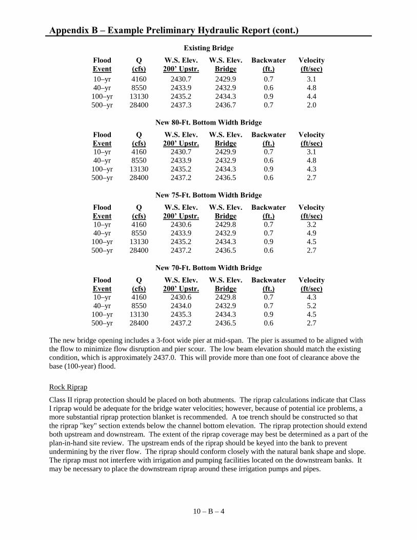
Appendix B � Example Preliminary Hydraulic Report (cont.)
10 – B – 4
Existing Bridge
Flood Event
Q (cfs)
W.S. Elev. 200� Upstr.
W.S. Elev. Bridge
Backwater(ft.)
Velocity (ft/sec)
10–yr 4160 2430.7 2429.9 0.7 3.1 40–yr 8550 2433.9 2432.9 0.6 4.8 100–yr 13130 2435.2 2434.3 0.9 4.4 500–yr 28400 2437.3 2436.7 0.7 2.0
New 80-Ft. Bottom Width Bridge
Flood Event
Q (cfs)
W.S. Elev. 200� Upstr.
W.S. Elev. Bridge
Backwater(ft.)
Velocity (ft/sec)
10–yr 4160 2430.7 2429.9 0.7 3.1 40–yr 8550 2433.9 2432.9 0.6 4.8 100–yr 13130 2435.2 2434.3 0.9 4.3 500–yr 28400 2437.2 2436.5 0.6 2.7
New 75-Ft. Bottom Width Bridge
Flood Event
Q (cfs)
W.S. Elev. 200� Upstr.
W.S. Elev. Bridge
Backwater(ft.)
Velocity (ft/sec)
10–yr 4160 2430.6 2429.8 0.7 3.2 40–yr 8550 2433.9 2432.9 0.7 4.9 100–yr 13130 2435.2 2434.3 0.9 4.5 500–yr 28400 2437.2 2436.5 0.6 2.7
New 70-Ft. Bottom Width Bridge
Flood Event
Q (cfs)
W.S. Elev. 200� Upstr.
W.S. Elev. Bridge
Backwater(ft.)
Velocity (ft/sec)
10–yr 4160 2430.6 2429.8 0.7 4.3 40–yr 8550 2434.0 2432.9 0.7 5.2 100–yr 13130 2435.3 2434.3 0.9 4.5 500–yr 28400 2437.2 2436.5 0.6 2.7
The new bridge opening includes a 3-foot wide pier at mid-span. The pier is assumed to be aligned with the flow to minimize flow disruption and pier scour. The low beam elevation should match the existing condition, which is approximately 2437.0. This will provide more than one foot of clearance above the base (100-year) flood.
Rock Riprap
Class II riprap protection should be placed on both abutments. The riprap calculations indicate that Class I riprap would be adequate for the bridge water velocities; however, because of potential ice problems, a more substantial riprap protection blanket is recommended. A toe trench should be constructed so that the riprap "key" section extends below the channel bottom elevation. The riprap protection should extend both upstream and downstream. The extent of the riprap coverage may best be determined as a part of the plan-in-hand site review. The upstream ends of the riprap should be keyed into the bank to prevent undermining by the river flow. The riprap should conform closely with the natural bank shape and slope. The riprap must not interfere with irrigation and pumping facilities located on the downstream banks. It may be necessary to place the downstream riprap around these irrigation pumps and pipes.

Appendix B � Example Preliminary Hydraulic Report (cont.)
10 – B – 5
Scour
Contraction, pier, and abutment scour were calculated for the 10, 40, 100, and 500-year flood events. The largest scour depths occur at the 40-year (road overtopping) flood event. As flood flows increase, a larger proportion of the flow overtops the road, resulting in decreased flow through the bridge opening. Thus, scour depths calculated for the 100 and 500-year events are equal to or less than those for the 40-year event. The results of the scour analyses are presented in the following table:
Abutment Scour (ft) Flow Frequency
Contraction Scour (ft)
Pier Scour (ft) Left Right
10–yr 2 6 None None 40–yr 4 7 7 10
Irrigation
There are no apparent irrigation ditches affected by the bridge or approach roads. There are pumping and intake facilities located on both banks downstream from the bridge. These facilities, including any appurtenant electrical lines or panels, must be protected and preserved during the project. Also, the irrigation "check dam" across the river below the bridge should not be disturbed during construction activities.
Recommendations
An 80-foot wide channel bottom (at elevation 2415.9) with 2H:1V spill-through abutments is the recommended bridge opening. The Station for the center of the channel section is 33+90. It is assumed that a 3-foot wide pier will be placed at mid-opening. The pier should be aligned with the river flow.
A low beam elevation of 2437.0, which nearly matches the existing condition, will provide more than one foot of clearance during the 100-year flood event. The existing approach road grades should be maintained to provide overflow relief for the bridge at flood events exceeding the 40-year frequency. It will probably be necessary to raise the road profile at both ends of the bridge to accommodate the increased beam/deck thickness. This raised road section should be kept as short as possible.
Class II riprap should be placed on both spill-through abutments, and extended upstream and downstream. The riprap should have a toe trench below the channel bottom and should be keyed into the bank on the upstream end. The downstream riprap should be placed to protect, but not hinder, the existing irrigation pumps and pipe intakes.

Appendix C � Example Bridge Opening Recommendation Memo
10 – C – 1
After the preliminary hydraulic report is prepared, a memo is sent to the Bridge Bureau recommending a bridge opening. This Appendix provides an example memo and an example scour sketch. The scour sketch (Figure 10-C-1) shows the location to be used to measure abutment scour. When available, core logs should also be shown on the scour sketch. The 2-year flow and stage are included as information for Environmental Services, for their use in obtaining COE Section 404 permits. The bridge opening recommendation is based on a trapezoidal section for simplicity, but the water surface profile model should include the natural channel bottom. The construction of the new bridge should not include excavation to the trapezoidal section (See Figure 10-C-2). The channel bottom elevation noted can be either the low point in the channel or the average channel bottom elevation.
Memorandum To: Bridge Engineer From: Hydraulics Engineer Date: August 30, 1994 Subject: BR 9003(16)
Milk River 1 Mile North of Lohman CN 2284
This memo presents our recommendations for the new structure over the Milk River for the subject project. The original plan for this replacement was to move an existing bridge on Highway 2 east of Lohman to this site. However, we now understand that this move is no longer feasible, and a new structure is planned for this crossing. The recommendations contained herein assume that the horizontal alignment will be maintained for the new structure.
Drainage Area 6166 square miles (15,970 sq.km.) Centerline of Channel Station 33+90 Channel Bottom Width 80 feet (24.4 meters) Channel Bottom Elevation 2415.9 feet MSL (736.4 meters) Channel Slope 0.00040 ft/ft (m/m) Trial Design Flow (10-yr) 4160 cfs (117.8 m3/s) Trial Design Stage Elev. 2430.7 feet MSL* (740.9 meters) Trial Design Velocity 3.1 ft/sec (0.95 m/sec) Trial Design Backwater 0.7 ft. (0.21 meter) Overtopping Flow (40-yr) 8550 cfs (242.1 m3/s) Overtopping Stage Elev. 2433.9 feet MSL* (741.9 meters) Overtopping Velocity 4.8 ft/sec (1.46 m/sec) Overtopping Backwater 0.6 ft. (0.18 meter) Base Flood (100-yr) 13130 cfs (371.8 m3/s) Base Flood Stage Elev. 2435.2 feet MSL* (742.3 meters) Base Flood Velocity 4.3 ft/sec (1.31 m/sec) Base Flood Backwater 0.9 ft. (0.27 meter) 500-year Flow 28400 cfs (804.2 m3/s) 500-year Backwater 0.6 ft. (0.18 meter)

Appendix C � Example Bridge Opening Recommendation Memo (cont.)
10 – C – 2
2-year Flow 1700 cfs (48.1 m3/s) 2-year Stage Elev. 2425.0 feet MSL* (739.1 meters) Skew 27 Degrees Bank Protection Class II Riprap Abutment Slope 2H:1V Low Beam Elevation 2437.0 feet MSL (742.8 meters)
*Water surface elevations are 200 feet upstream from the bridge. Water surface elevations include backwater, and include effects of a 3-foot pier placed at mid-channel and aligned with the flow. Velocities shown are at the downstream face of the bridge. The approach roadways are overtopped at the 40-year frequency flood event (8550 cfs). Scour depth calculations for this event and for the 10, 100, and 500-year flood events were completed. Maximum scour depths occur at the 40-year road overtopping event. As flood flows increase beyond this event, a larger proportion of the flow overtops the approach roads , while flow through the bridge opening decreases, resulting in lower scour depths at the larger flood events. Scour depths for the 10 and 40-year (roadway overtopping) flood events are presented in the following table.
Abutment Scour (ft) Flow Frequency
Contraction Scour (ft)
Pier Scour (ft) Left Right
10–yr 2 (0.6 m) 6 (1.8 m) None None 40–yr 4 (1.2 m) 7 (2.1 m) 7 (2.1 m) 10 (3.1 m)
A sketch of the potential scour for the 40-year roadway overtopping flood event is attached. The riprap on the abutments will serve as a countermeasure for the potential abutment scour, and therefore the abutment scour will be less than that predicted. The top of the pier footing should be set below the predicted 7 feet of pier scour. The pier scour is based on a 3-foot wide pier aligned with the flow. If the pier cannot be aligned with the flow, new scour calculations will be necessary. A copy of the Preliminary Hydraulics Report is also attached. c: Preconstruction Engineer Hydraulics Engineer District Administrator Road Design Engineer Geotechnical Engineer Environmental Services

Appendix C � Example Bridge Opening Recommendation Memo (cont.)
10 – C – 3
Figure 10�C�1 Scour Sketch
The above sketch shows the maximum potential scour for the recommended bridge opening. This sketch includes contraction scour, abutment scour and pier scour. It also indicates the location that each of these is measured. Note that the abutment scour (added to the contraction scour) is measured from a point on the abutment slope a distance ya (the average depth of flow in the overbank) below the water surface. The abutment scour cone is plotted at an angle of repose of 40����, and the pier scour cone is plotted with a width equal to two times the pier scour depth, on each side of the pier. The above sketch reflects a constant contraction scour elevation. At some sites, it may be more appropriate for the contraction scour to be shown parallel to the channel bottom.

Appendix C � Example Bridge Opening Recommendation Memo (cont.)
10 – C – 4
Figure 10�C�2
Appendix D � Procedure Memorandums
10 – D – 1
There are three procedure memorandums that have been issued that are relevant to bridge crossings. These are PM No. 8, issued November 1, 1983, PM No. 13 issued September 11, 1984, and Interim PM No. 14, issued September 21, 1989. Procedure Memorandum No. 8 is shown below, with some minor modifications.
Procedure Memorandum No. 13 relates to Location Hydraulic Reports for Bridge Replacement Type Projects. This Procedure Memorandum was written primarily to reduce the level of detail necessary in Location Reports written for single site bridge replacements. Standard procedure for MDT now is to write a Location Report, as described in Procedure Memorandum No. 1 or No 2, for all bridge replacement projects.
Interim Procedure Memorandum No. 14 relates to bridge scour determination. This Interim PM was issued shortly after FHWA issued the first Technical Advisory on scour. The procedures described in Interim PM No. 14 have been superseded by HEC-18 and by the scour calculation discussions in this Chapter.
PROCEDURE MEMORANDUM NO. 8 Date: November 1, 1983 BRIDGE CROSSINGS Updated: July 1997 GENERAL This memorandum outlines procedures for documenting the design process for bridge crossings. PROCEDURES
1 - Prior to alignment and grade review, preliminary bridge opening recommendations shall be submitted to the Bridge Bureau with a copy provided to the section responsible for developing road plans. These recommendations shall include hydraulic data listing drainage area and the magnitude, high water elevation, and velocity for the design flood, base flood, overtopping flood and 2-year flood. Any special requirements which have been considered or are known at this stage such as guide banks, riprap or overflow sections shall also be reported. Design information developed shall be summarized in a Hydraulic Report, to include information in Form HYD 4, Part 1 and supplemented with the Drainage Crossing Risk Assessment (Form HYD 4, Part 2, see Appendix A, Hydrology Chapter).
2 - Any necessary modifications to the preliminary recommendations, hydraulic data, or special requirements shall be submitted after final road grades have been established and preliminary bridge general layouts have been reviewed. Documentation in the design files, including the Drainage Crossing Hydraulic Report and Drainage Crossing Risk Assessment shall be reviewed and modified as necessary to assure accuracy.
3 - After plan-in-hand inspection, the hydraulic data shall be included on the Hydraulic Data Summary Sheet (see Appendix H, Culvert Chapter).

Appendix D � Procedure Memorandums (continued)
10 – D – 2
PROCEDURE MEMORANDUM NO. 13 Date: September 11, 1984 LOCATION REPORTS (Bridge Replacement Type Projects) Revised: July 1997 GENERAL The requirements for Location Hydraulics Studies and Reports are discussed in Procedure Memorandums No. 1 and No. 2. This Procedure Memorandum includes a procedure that can be used for the Field Review of Bridge Replacement Type Projects to identify the pertinent issues. The attached Form HYD 6 can be used to assist in collection of the necessary data. PROCEDURE 1. Items 1 through 6 should be completed as much as possible and practical prior to attending
the field review so the designer can have an idea of what to expect or look for.
a. Preliminary hydrology may be merely by USGS Regression Equations.
b. Headwaters location shall be by Corps of Engineers list (when listed).
2. Items 7 and 8 shall reflect any anticipated channel changes or encroachments with various alternates and brief discussion of why they cannot be avoided. (If necessary, discussions may be continued under item 12.)
3. Items 9 and 11 shall provide data on possible backwater damages, overflow relief and potential problems that may arise due to grade and alignment changes (i.e., replacing a truss bridge with a girder bridge, etc.).
4. Item 10 shall provide information concerning the possibility of using culverted detours, even if only during short periods of the year, and the desirable location.
5. Item 12 shall provide a discussion of possible impacts or design constraints. Included in this section should be a discussion of potential water quality impacts (as related to temporary fill in the channel for detours, channel changes, grade control structures, etc.).
6. Item 13 should document that hydraulic related impacts are minor.
7. Item 14 shall be used to note when other than the full HYD 1 survey is required (e.g., culvert will be adequate and only a couple typical channel sections and channel bottom or water surface profiles are needed; bridge crossing will be square, is well defined, and contour map is not necessary; etc.).

Appendix D � Procedure Memorandums (continued)
10 – D – 3
FORM HYD 6 Page 1 of 2 Revised May 1997
FIELD REVIEW AND LOCATION HYDRAULICS DATA SHEET
Project Name Project Number Designer Date of Review 1. LOCATION
2. EXISTING STRUCTURE
3. DRAINAGE AREA
4. PRELIMINARY HYDROLOGY
Frequency Range of Flows 10 yr. 25 yr. 50 yr. 100 yr.
5. DETERMINATION OF NEED FOR SECTION 404 PERMIT
Is the crossing below headwaters? Estimated flow on date of review?
6. IS THIS A DELINEATED FLOODPLAIN? Approximate Study Detailed Study Panel Number Is county regulating floodplains?
7. CHANNEL MODIFICATIONS
8. ANY LONGITUDINAL FLOODPLAIN ENCROACHMENTS? Are there practicable alternatives that would avoid floodplain encroachments?
9. RISK Can roadway be overtopped? Potential backwater damages
10. CONSTRUCTION DETOUR Upstream Downstream Bridge Pipe
11. PROPOSED ALIGNMENT Horizontal Vertical

Appendix D � Procedure Memorandums (continued)
10 – D – 4
FORM HYD 6 Page 2 of 2 Revised May 1997 12. ADDITIONAL IMPACTS AND REMARKS
(Include comments on Channel Stability, Flood History, Fisheries, Utilities, Irrigation, Ice and Debris, etc.)
13. ARE IMPACTS MINIMAL?
14. HYDRAULIC SURVEY REQUIREMENTS

Appendix E � Plan Form Changes
10 – E – 1
Plan form changes are morphological changes such as meander migration or channel braiding. The lateral movement of meanders can threaten bridge approaches as well as increase scour by changing flow patterns approaching a bridge opening. A braided channel can cause significant changes in the flow distribution and thus the bridge's flow contraction ratio. Some examples of plan form changes and the possible effects, taken from �Highways in the River Environment,� are included in this appendix.
(1) Crossing downstream of an alluvial fan
Local Effects 1. Fan reduces waterway 2 Direction of flow at bridge site is uncertain 3 Channel location is uncertain
Upstream Effects 1 Erosion of banks 2 Unstable channel 3 Large transport rates
Downstream Effects 1 Aggradation 2 Flooding 3 Development of tributary bar in the main channel
Figure 10�E�1

Appendix E � Plan Form Changes (continued)
10 – E – 2
(2) Lowering of base level for the channel
Local Effects 1 Headcutting 2 General scour 3 Local scour 4 Bank instability 5 High velocities
Upstream Effects 1 Increased velocity 2 Increased bed material transport 3 Unstable channel 4 Possible change of form of river
Downstream Effects 1 Increased transport to main channel 2 Aggradation 3 Increased flood stage
Figure 10�E�2
(3) Channel Characterized by prolonged low flows
Local Effects 1 At low flow a low water channel develops in river bed 2 Increased danger to piers due to channelization and local scour 3 Bank caving
Figure 10�E�3

Appendix E � Plan Form Changes (continued)
10 – E – 3
(4) Cutoffs downstream of crossing
Local Effects 1 Steeper slope 2 Higher velocity 3 Increased transport 4 Degradation and possible headcutting 5 Banks unstable 6 River may braid 7 Danger to bridge foundation from degradation and local scour
Upstream Effects See Local Effects
Downstream Effects 1 Deposition downstream of straightened channel 2 Increase in flood stage 3 Loss of channel capacity 4 Degradation in tributary
Figure 10�E�4

Appendix E � Plan Form Changes (continued)
10 – E – 4
(5) Excess of sediment at bridge site due to upstream tributary.
Local Effects 1 Contraction of the river 2 Increased velocity 3 General and local scour 4 Bank instability
Upstream Effects 1 Aggradation 2 Backwater at flood stage 3 Changed response of the tributary
Downstream Effects 1 Deposition of excess sediment eroded at and downstream of the bridge 2 More severe attack at first bend downstream 3 Possible development of a chute channel across the second point bar
downstream of the bridge
Figure 10�E�5
sleep tributary
closed

Appendix E � Plan Form Changes (continued)
10 – E – 5
(6) River channel relocation at crossing site
Local Effects 1 None if straight section is designed to transport the sediment load of
the river and if it is designed to be stable when subjected to anticipated flow. Otherwise same as in case (4).
Upstream Effects 1 Similar to local effects
Downstream Effects 1 Similar to local effects
Figure 10�E�6

Appendix E � Plan Form Changes (continued)
10 – E – 6
Figure 10�E�7
(7) Raising of river base level
Local Effects 1 Aggradation of bed 2 Loss of waterway 3 Change in river geometry 4 Increased flood stage
Upstream Effects 1 See local effects 2 Change in base level for tributaries 3 Deposition in tributaries near confluences 4 Aggradation causing a perched river channel
to develop or changing the alignment of the main channel
Downstream Effects 1 See upstream effects
Increased stage

Appendix E � Plan Form Changes (continued)
10 – E – 7
(8) Reduction of Sediment Load Upstream
Local Effects 1 Channel degradation 2 Possible change in river form 3 Local scour 4 Possible bank instability 5 Possible destruction of structure due to dam failure
Upstream Effects 1 Degradation 2 Reduced flood stage 3 Reduce base level for tributaries, increased velocity and reduced
channel stability causing increased sediment transport to main channel
Downstream Effects 1 Degradation 2 Increased velocity and transport in tributaries
Figure 10�E�8

Appendix E � Plan Form Changes (continued)
10 – E – 8
(9) Naturally shifting river channel
Local Effects 1. Rivers are dynamic (ever changing) and the
rate of change with time should be evaluated as part of the geomorphic and hydraulic analysis
2. Alignment of main channel continually changes affecting alignment of flow with respect to Bridge A
3. If the main channel shifts to the alternate position, the confluence shifts and the tributary gradient is significantly increased causing degradation in the tributary. Local effects on Bridge B same as in 1, 2, 3 and 4 in Case (8).
4. Excess sediment from the tributary, assuming (3) causes aggradation in the main channel and possible significant changes in channel alignment
Upstream Effects 1 The river could abandon its present channel.
Changing position of the main channel may require realignment of training works.
Downstream Effects 1 See upstream effects 2 Shifts in the position of the main channel
relative to the position of the confluence with the tributary alternatively flattens or steepens the gradient of the tributary causing corresponding aggradation and degradation.
3 Shifts in the position of the main channel causes aggradation, degradation and instabilities depending upon direction and magnitude of channel change
Figure 10�E�9

Appendix E � Plan Form Changes (continued)
10 – E – 9
(10) Man–induced reduction of channel length
Local Effects 1 Bridge A is first subjected to
degradation and then aggradation 2 Bridge B is primarily subjected to
degradation. The magnitude can be large.
3 The whole system is subjected to passage of sediment waves.
4 River form could change to braided. 5 Flood levels are reduced at B and
increased at A 6 Local and general scour is significantly
affected.
Upstream Effects 1 A change of river form from
meandering to braiding is possible. 2 Rate of sediment transport is
increased. 3 Head cutting is induced in the whole
system. 4 Flood stage is reduced. 5 Velocity increase 6 Tributaries respond to main channel
changes.
Downstream Effects 1 For Bridge B see upstream effects. 2 For Bridge A the channel first
degrades then significantly aggrades. 3 Large quantities of bed material and
wash load are carried to the reservoir.
4 Delta forms in the reservoir. 5 Wash load may affect water quality in
the entire reservoir. 6 Tributaries respond to main channel
changes.
Figure 10�E�10

Appendix E � Plan Form Changes (continued)
10 – E – 10
(11) Earthquakes
Local Effects 1 Channel changes 2 Scour or deposition 3 Decrease in bank stability 4 Landslides 5 Rockslides 6 Mudflows
Upstream Effects 1 See local effects 2 Slide lakes
Downstream Effects 1 See local effects 2 Slide lakes
Figure 10�E�11
Uplift or Lateral Shift

Appendix E � Plan Form Changes (continued)
10 – E – 11
(12) Longitudinal Encroachment
Local Effects 1 Increased energy gradient and potential bank and bed scour 2 Highway fill is subject to scour as channel tends to shift to old
alignment 3 Reach is subject to bed degradation as headcut develops at the
downstream and travels upstream 4 Lateral drainage into the river is interrupted and may cause flooding and
erosion
Upstream Effects 1 Energy gradient also increased in the reach upstream and may cause
change of river form from meandering to braided 2 Rate of sediment transport is increased. As the headcut travels
upstream severe bank and bed erosion is possible. 3 If tributaries in the zone of influence exist, they will respond to
lowering of based level.
Downstream Effects 1 Channel will aggrade as the sediment load coming from bed and bank
erosion is received 2 Channel may deteriorate from meandering to braided
Figure 10�E�12

Appendix E � Plan Form Changes (continued)
10 – E – 12
(13) Longitudinal Encroachment
Local Effects 1 Reduced waterway causes a local obstruction to flow and higher
velocities. 2 Significant erosion problem on the highway fill and induced bed
degradation 3 Lateral drainage into the river is interrupted and may cause flooding and
erosion
Upstream Effects 1 Backwater generated by the obstruction increases flood stage 2 Deposition induced by the backwater
Downstream Effects 1 Large sediment load may cause aggradation 2 Local scour at end of contracted section
Figure 10�E�13

Appendix E � Plan Form Changes (continued)
10 – E – 13
(14) Longitudinal Encroachment
Local Effects 1 Erosion of highway fill and submergence possible during floods 2 Patterns of overbank spill are affected by the encroachment and in
highly shifting channels may change river course downstream 3 Lateral drainage into river is interrupted and may cause flooding and
erosion
Upstream Effects 1 If significant encroachment on the floodplain waterway, backwater may
be induced
Downstream Effects 1 If the river channel is highly shifting, the channel alignment may change 2 If significant erosion experienced upstream, aggradation will occur
Figure 10�E�14

Appendix F Detour Guidelines
10 – F – 1
On some bridge crossings, the Construction Bureau requests pipe sizes for detours. When MDT specifies the size of the detour pipe, MDT assumes the liability if a larger flood occurs during construction and damages the work. The Contractor is forced to use the size of pipe specified, even though the work schedule may allow for the detour to be in place only during the �dry� time of year, when a much smaller pipe may be very adequate. The information provided to the Construction Bureau should be based on the criteria below, although by scheduling the detour installation after the peak runoff the structure could be smaller. On the other hand, by sizing the detour for a 2-year event, there is a 50% risk that this event will be exceeded in any year. The Contractor is probably in the best position to assess the risk. In order to maintain consistency, detour pipes will be sized based on the following criteria.
1. Determine 2-year flood flow, using the same hydrologic method used to determine the design flow. This will be the design flow for detours.
2. Determine the minimum-sized pipe(s) that will pass this design flow with HW/D less than or equal to 1.0. Also, determine the number of 48" pipes that are necessary to pass this design flow.
A memo will be written to the Construction Engineer stating the size of pipe(s) required to pass the 2-year flow and the number of 48" pipes required to pass the 2-year flow.