chapter 14 markets for factor inputs. chapter 14slide 2 topics to be discussed competitive factor...
TRANSCRIPT
Chapter 14
Markets for Factor InputsMarkets for
Factor Inputs

Chapter 14 Slide 2
Topics to be Discussed
Competitive Factor Markets
Equilibrium in a Competitive Factor Market
Factor Markets with Monopsony Power
Factor Markets with Monopoly Power
Chapter 14 Slide 3
Competitive Factor Markets
Characteristics
1) Large number of sellers of the factor of production
2) Large number of buyers of the factor of production
3) The buyers and sellers of the factor of production are price takers

Chapter 14 Slide 4
Competitive Factor Markets
Demand for a Factor Input When Only One Input Is VariableDemand for factor inputs is a derived
demand…derived from factor cost and output
demand
Chapter 14 Slide 5
Competitive Factor Markets
AssumeTwo inputs: Capital (K) and Labor (L)Cost of K is r and the cost of labor is wK is fixed and L is variable
Demand for a Factor Input WhenOnly One Input Is Variable
Demand for a Factor Input WhenOnly One Input Is Variable
Chapter 14 Slide 6
Competitive Factor Markets
ProblemHow much labor to hire
Demand for a Factor Input WhenOnly One Input Is Variable
Demand for a Factor Input WhenOnly One Input Is Variable
Chapter 14 Slide 7
Competitive Factor Markets
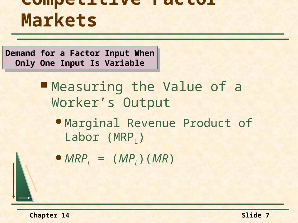
Measuring the Value of a Worker’s OutputMarginal Revenue Product of Labor
(MRPL)
MRPL = (MPL)(MR)
Demand for a Factor Input WhenOnly One Input Is Variable
Demand for a Factor Input WhenOnly One Input Is Variable
Chapter 14 Slide 8
Competitive Factor Markets
Assume perfect competition in the product marketThen MR = P
Demand for a Factor Input WhenOnly One Input Is Variable
Demand for a Factor Input WhenOnly One Input Is Variable
Chapter 14 Slide 9
Competitive Factor Markets
Question
What will happen to the value of MRPL when more workers are hired?
Demand for a Factor Input WhenOnly One Input Is Variable
Demand for a Factor Input WhenOnly One Input Is Variable
Chapter 14 Slide 10
Marginal Revenue Product
Hours of Work
Wages($ perhour)
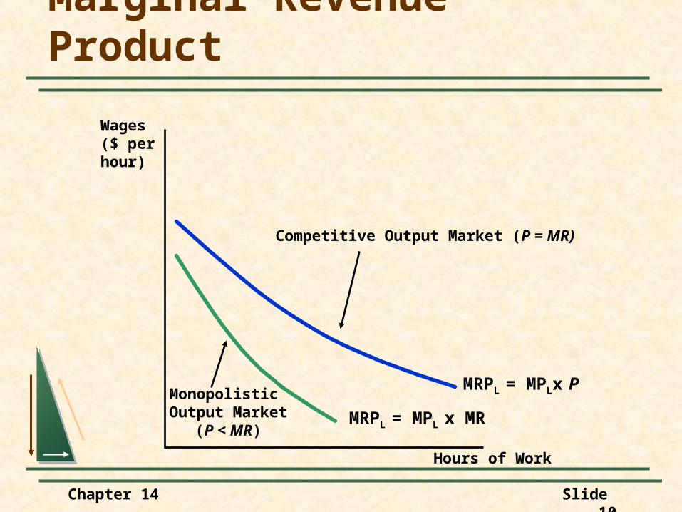
MRPL = MPLx P
Competitive Output Market (P = MR)
MRPL = MPL x MR
Monopolistic Output Market
(P < MR)
Chapter 14 Slide 11
Competitive Factor Markets
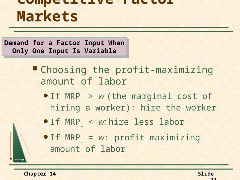
Choosing the profit-maximizing amount of labor
If MRPL > w (the marginal cost of hiring a worker): hire the worker
If MRPL < w: hire less labor
If MRPL = w: profit maximizing amount of labor
Demand for a Factor Input WhenOnly One Input Is Variable
Demand for a Factor Input WhenOnly One Input Is Variable
Chapter 14 Slide 12
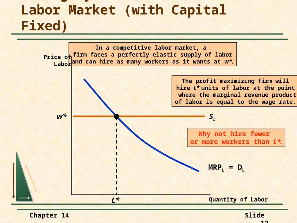
w* SL
In a competitive labor market, a firm faces a perfectly elastic supply of labor
and can hire as many workers as it wants at w*.
Hiring by a Firm in theLabor Market (with Capital Fixed)
Quantity of Labor
Price ofLabor
Why not hire fewer or more workers than L*.
MRPL = DL
L*
The profit maximizing firm willhire L* units of labor at the point
where the marginal revenue productof labor is equal to the wage rate.
Chapter 14 Slide 13
Competitive Factor Markets
If the market supply of labor increased relative to demand (baby boomers or female entry), a surplus of labor would exist and the wage rate would fall.
QuestionHow would this impact the quantity
demanded for labor?
Demand for a Factor Input WhenOnly One Input Is Variable
Demand for a Factor Input WhenOnly One Input Is Variable

Chapter 14 Slide 14
A Shift in the Supply of Labor
Quantity of Labor
Price ofLabor
w1S1
MRPL = DL
L1
w2
L2
S2
Chapter 14 Slide 15
Competitive Factor Markets
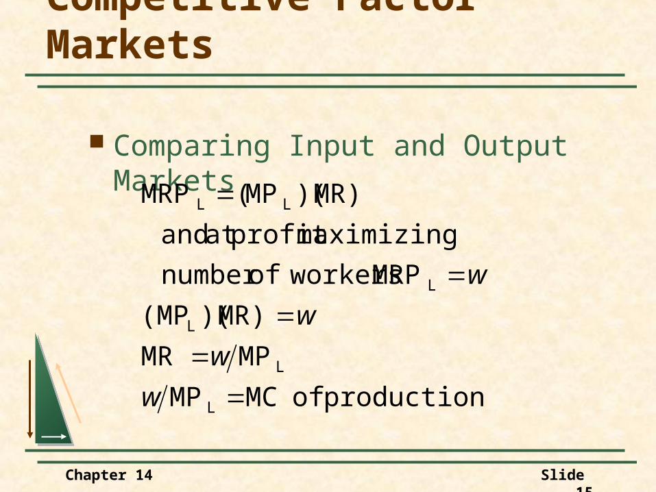
Comparing Input and Output Markets
production of MC MP
MP MR
MR))((MP
MRP workersofnumber
maximizingprofit at and
MR))(MP(MRP
L
L
L
L
LL
w
w
w
w
Chapter 14 Slide 16
Competitive Factor Markets
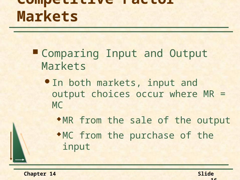
Comparing Input and Output MarketsIn both markets, input and output choices
occur where MR = MCMR from the sale of the outputMC from the purchase of the input
Chapter 14 Slide 17
Competitive Factor Markets
ScenarioProducing farm equipment with two
variable inputs:LaborAssembly-line machinery
Assume the wage rate falls
Demand for a Factor Input WhenSeveral Inputs Are Variable
Demand for a Factor Input WhenSeveral Inputs Are Variable
Chapter 14 Slide 18
Competitive Factor Markets
QuestionHow will the decrease in the wage rate
impact the demand for labor?
Demand for a Factor Input WhenSeveral Inputs Are Variable
Demand for a Factor Input WhenSeveral Inputs Are Variable
Chapter 14 Slide 19
MRPL1 MRPL2
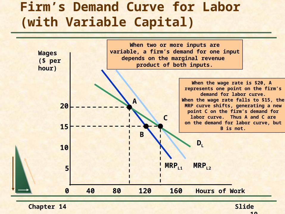
When two or more inputs arevariable, a firm’s demand for one input
depends on the marginal revenue product of both inputs.
Firm’s Demand Curve for Labor(with Variable Capital)
Hours of Work
Wages($ perhour)
0
5
10
15
20
40 80 120 160
When the wage rate is $20, A represents one point on the firm’s
demand for labor curve.When the wage rate falls to $15, theMRP curve shifts, generating a new
point C on the firm’s demand forlabor curve. Thus A and C are
on the demand for labor curve, butB is not.
DL
A
B
C
Chapter 14 Slide 20
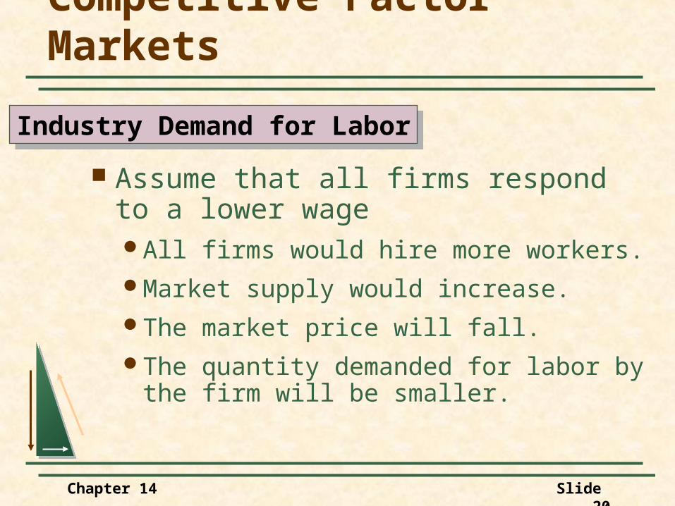
Assume that all firms respond to a lower wageAll firms would hire more workers.Market supply would increase.The market price will fall. The quantity demanded for labor by the
firm will be smaller.
Competitive Factor Markets
Industry Demand for LaborIndustry Demand for Labor
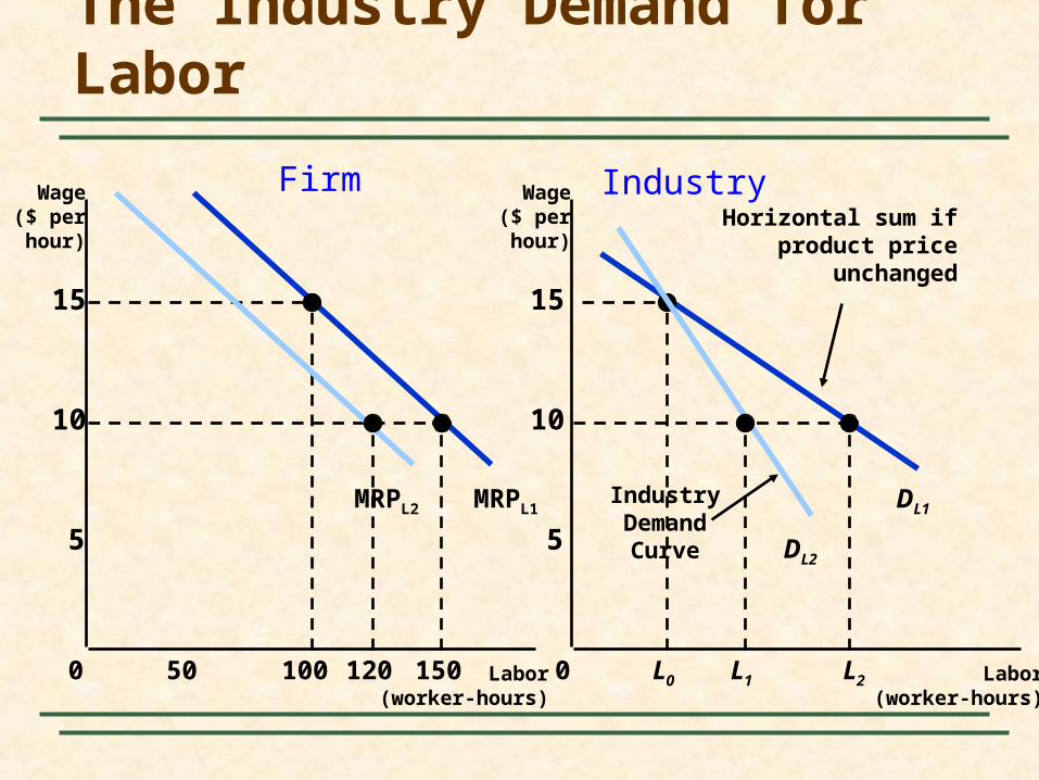
MRPL1
The Industry Demand for Labor
Labor(worker-hours)
Labor(worker-hours)
Wage($ perhour)
Wage($ perhour)
0
5
10
15
0
5
10
15
50 100 150 L0 L2
DL1
Horizontal sum ifproduct price
unchanged
120
MRPL2
L1
IndustryDemandCurve DL2
Firm Industry
Chapter 14 Slide 22
The Industry Demand for Labor
QuestionHow would a change to a non-competitive
market impact the derivation of the market demand for labor?
Chapter 14 Slide 23
The Demand for Jet Fuel
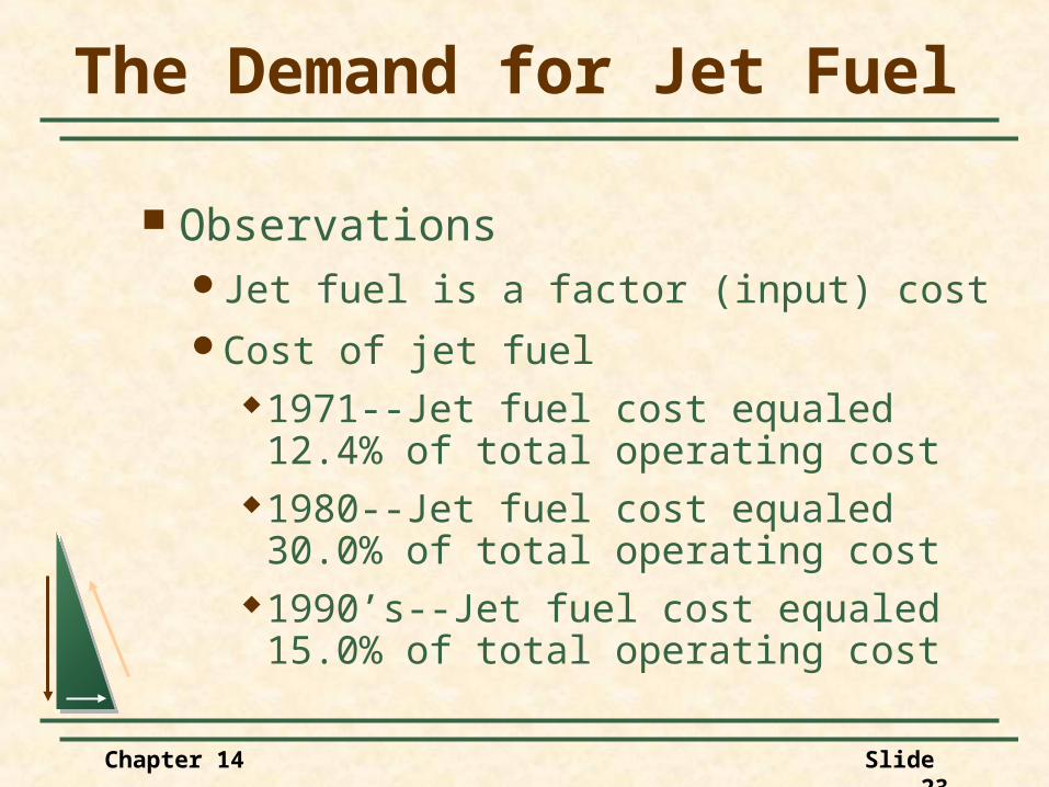
ObservationsJet fuel is a factor (input) costCost of jet fuel
1971--Jet fuel cost equaled 12.4% of total operating cost
1980--Jet fuel cost equaled 30.0% of total operating cost
1990’s--Jet fuel cost equaled 15.0% of total operating cost

Chapter 14 Slide 24
The Demand for Jet Fuel
ObservationsAirlines responded to higher prices in the
1970’s by reducing the quantity of jet fuel used
Ton-miles increased by 29.6% & jet fuel consumed rose by 8.8%

Chapter 14 Slide 25
The Demand for Jet Fuel
ObservationsThe demand for jet fuel impacts the airlines
and refineries alikeThe short-run price elasticity of demand for
jet-fuel is very inelastic
Chapter 14 Slide 26
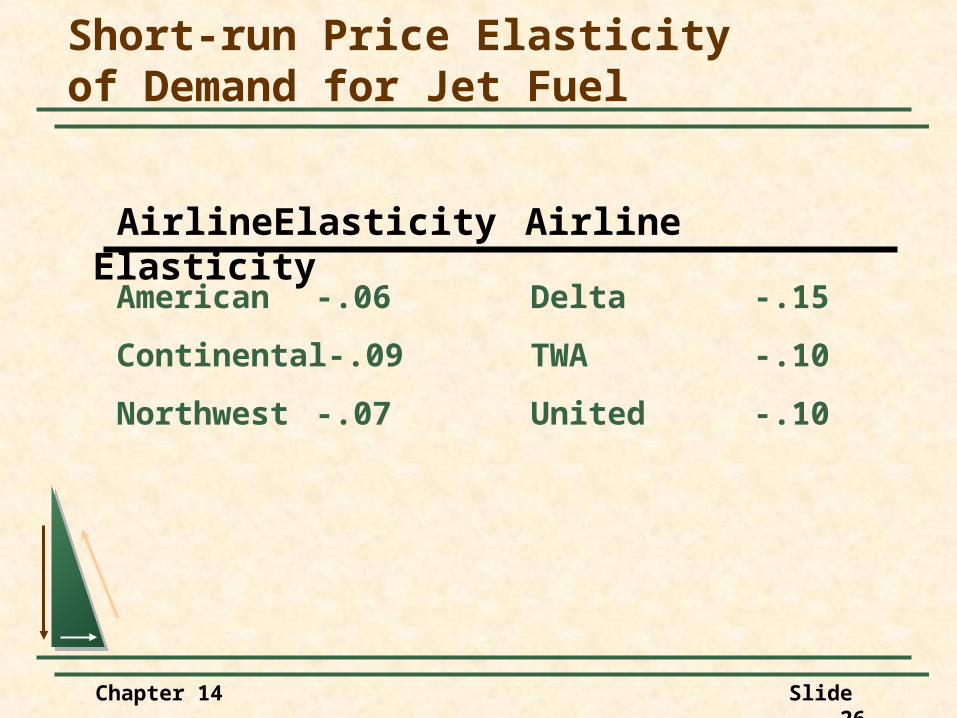
Short-run Price Elasticityof Demand for Jet Fuel
American -.06 Delta -.15
Continental -.09 TWA -.10
Northwest -.07 United -.10
Airline Elasticity Airline Elasticity
Chapter 14 Slide 27
The Demand for Jet Fuel
QuestionHow would the long-run price elasticity of
demand compare to the short-run?
Chapter 14 Slide 28
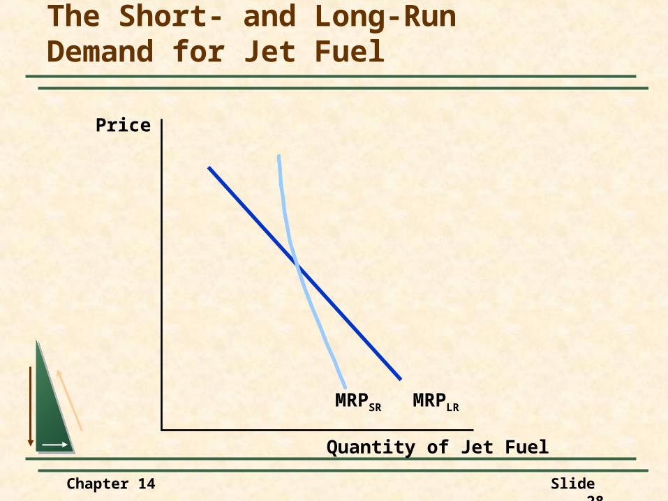
The Short- and Long-RunDemand for Jet Fuel
Quantity of Jet Fuel
Price
MRPLRMRPSR
Chapter 14 Slide 29
Competitive Factor Markets
The Supply of Inputs to a FirmDetermining how much of an input to
purchaseAssume a perfectly competitive factor
market

SMarket Supplyof fabric
A Firm’s Input Supply in aCompetitive Factor Market
Yards ofFabric (thousands)
Yards ofFabric (thousands)
Price($ peryard)
Price($ peryard)
D
Market Demandfor fabric
100
ME = AE10 10
Supply ofFabric Facing Firm
50
Demand for Fabric
MRP
Observations1) The firm is a price taker at $10.2) S = AE = ME = $103) ME = MRP @ 50 units
Chapter 14 Slide 31
Competitive Factor Markets
The Market Supply of InputsThe market supply for physical inputs is
upward slopingExamples: jet fuel, fabric, steel
The market supply for labor may be upward sloping and backward bending
Chapter 14 Slide 32
Competitive Factor Markets
The Supply of LaborThe choice to supply labor is based on
utility maximization
Leisure competes with labor for utility
Wage rate measures the price of leisure
Higher wage rate causes the price of leisure to increase
Chapter 14 Slide 33
Competitive Factor Markets
The Supply of LaborHigher wages encourage workers to
substitute work for leisure (i.e. the substitution effect)
Higher wages allow the worker to purchase more goods, including leisure which reduces work hours (i.e. the income effect)
Chapter 14 Slide 34
Competitive Factor Markets
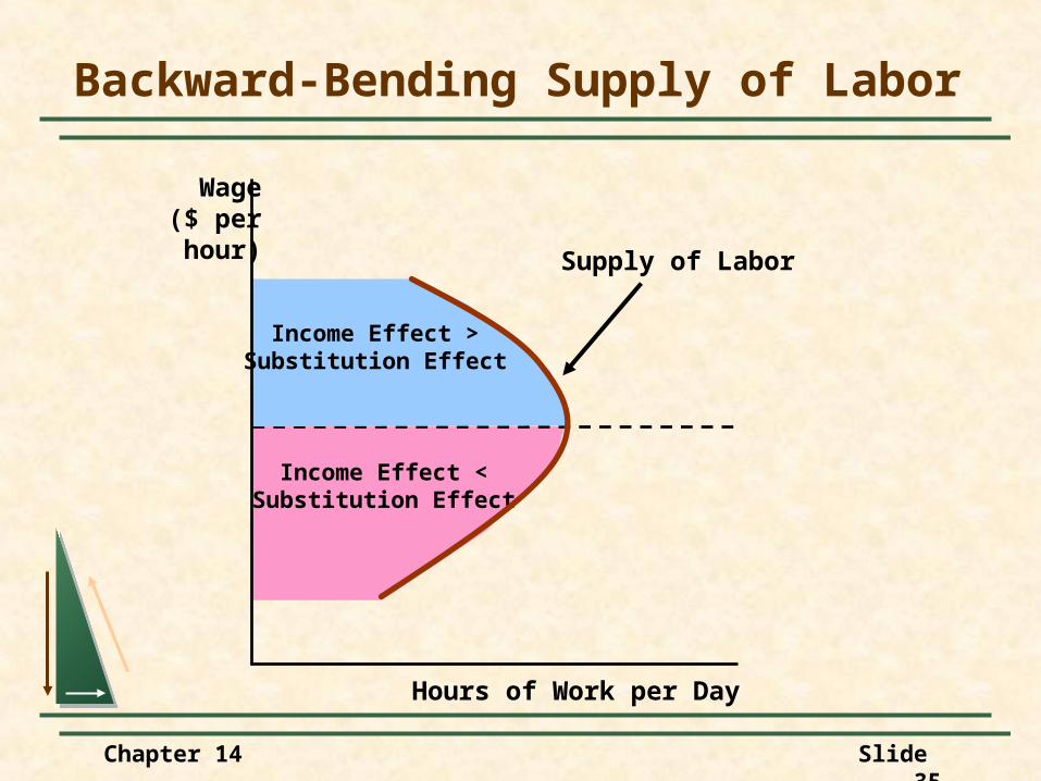
The Supply of LaborIf the income effect exceeds the
substitution effect the supply curve is backward bending
Chapter 14 Slide 35
Income Effect <Substitution Effect
Income Effect >Substitution Effect
Backward-Bending Supply of Labor
Hours of Work per Day
Wage($ perhour) Supply of Labor
12
C
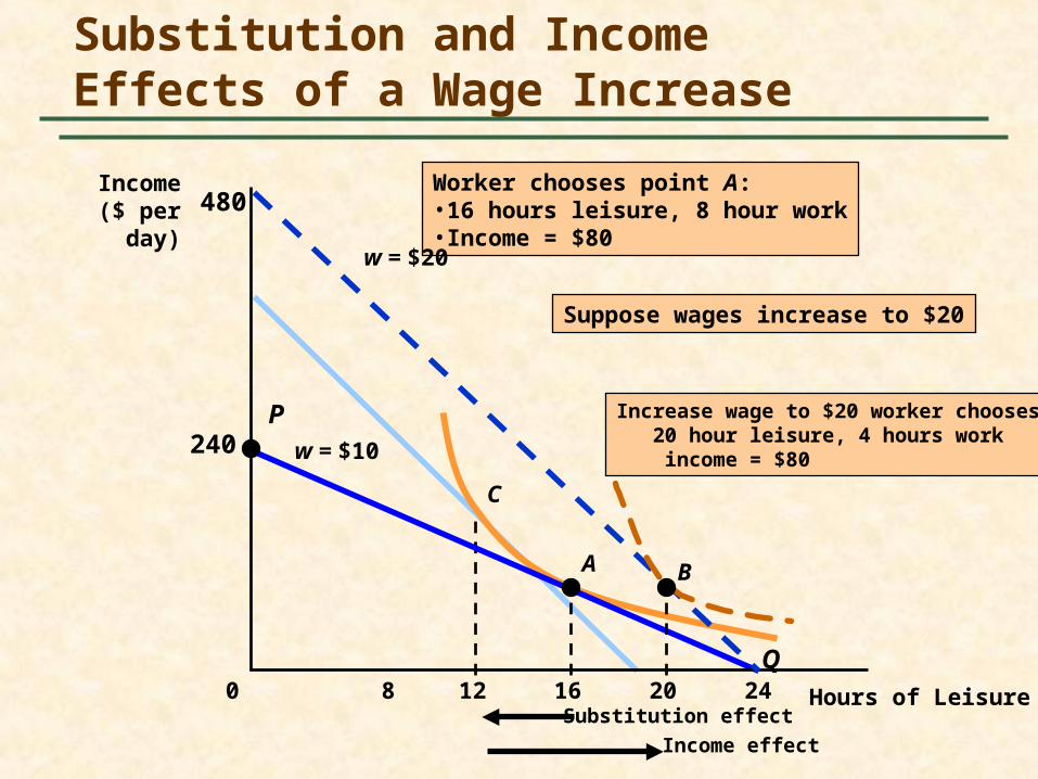
Worker chooses point A:•16 hours leisure, 8 hour work•Income = $80
16Q
P
A
w = $10
Substitution and IncomeEffects of a Wage Increase
Hours of Leisure
Income($ per
day)
0
240
8 24
480
20
B
w = $20
Suppose wages increase to $20
Substitution effect
Income effect
Increase wage to $20 worker chooses: 20 hour leisure, 4 hours work income = $80
Chapter 14 Slide 37
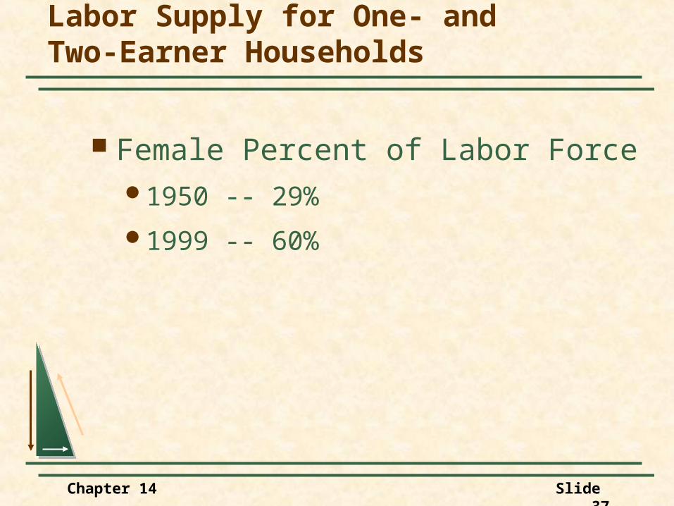
Labor Supply for One- andTwo-Earner Households
Female Percent of Labor Force1950 -- 29%
1999 -- 60%
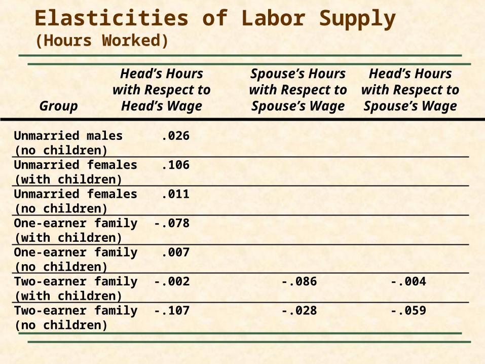
Elasticities of Labor Supply (Hours Worked)
Head’s Hours Spouse’s Hours Head’s Hourswith Respect to with Respect to with Respect to
Group Head’s Wage Spouse’s Wage Spouse’s Wage
Unmarried males .026(no children)Unmarried females .106(with children)Unmarried females .011(no children)One-earner family -.078(with children)One-earner family .007(no children)Two-earner family -.002 -.086 -.004(with children)Two-earner family -.107 -.028 -.059(no children)
Chapter 14 Slide 39
Equilibrium in aCompetitive Factor Market
A competitive factor market is in equilibrium when the price of the input equates the quantity demanded to the quantity supplied.
SL = AE
SL = AE
DL = MRPL DL = MRPL
P * MPL
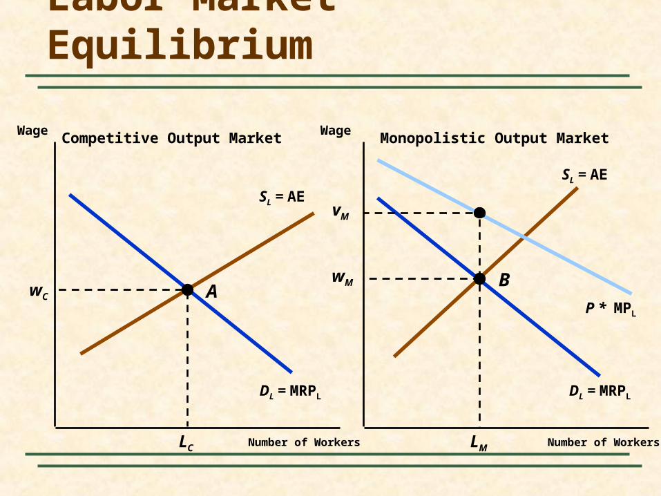
Labor Market Equilibrium
Number of Workers Number of Workers
Wage WageCompetitive Output Market Monopolistic Output Market
wC
LC
wM
LM
vM
AB
Chapter 14 Slide 41
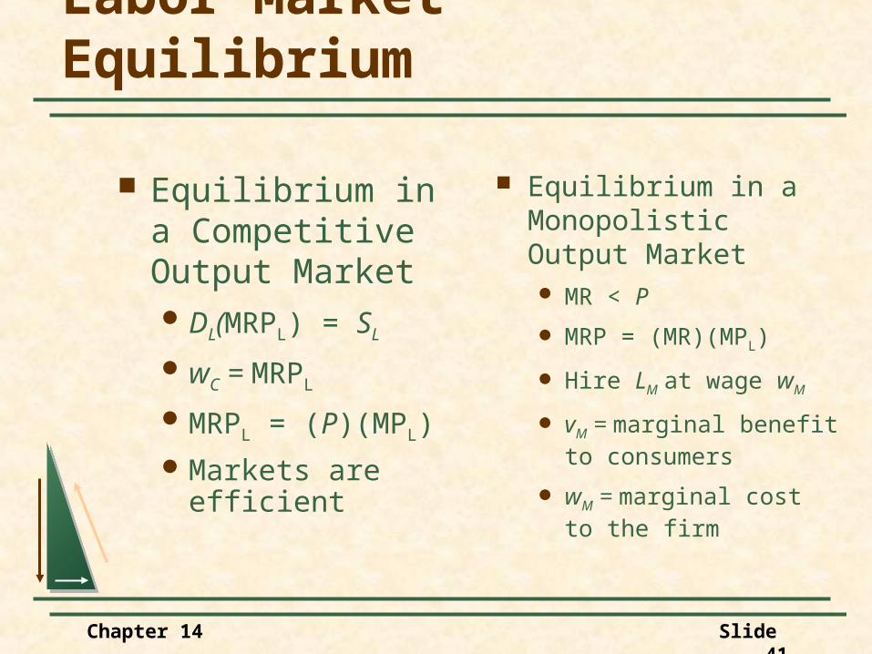
Labor Market Equilibrium
Equilibrium in a Competitive Output MarketDL(MRPL) = SL
wC = MRPL
MRPL = (P)(MPL)
Markets are efficient
Equilibrium in a Monopolistic Output Market MR < P
MRP = (MR)(MPL)
Hire LM at wage wM
vM = marginal benefit to consumers
wM = marginal cost to the firm
Chapter 14 Slide 42
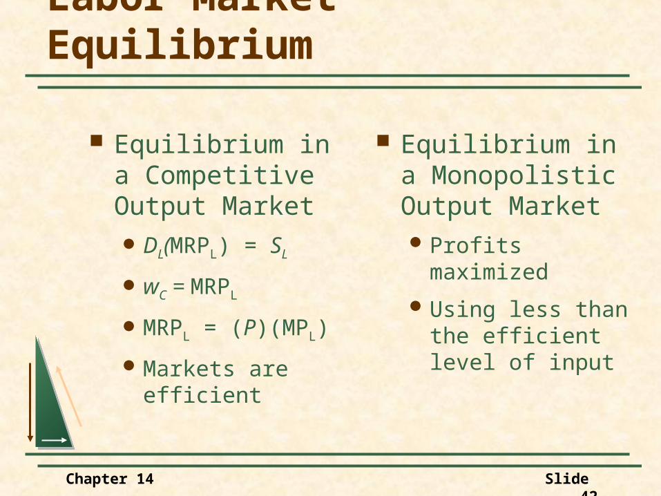
Labor Market Equilibrium
Equilibrium in a Competitive Output MarketDL(MRPL) = SL
wC = MRPL
MRPL = (P)(MPL)
Markets are efficient
Equilibrium in a Monopolistic Output MarketProfits maximized
Using less than the efficient level of input
Chapter 14 Slide 43
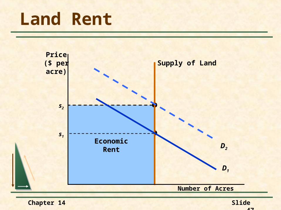
Economic RentFor a factor market, economic rent is the
difference between the payments made to a factor of production and the minimum amount that must be spent to obtain the use of that factor.
Equilibrium in aCompetitive Factor Market
Chapter 14 Slide 44
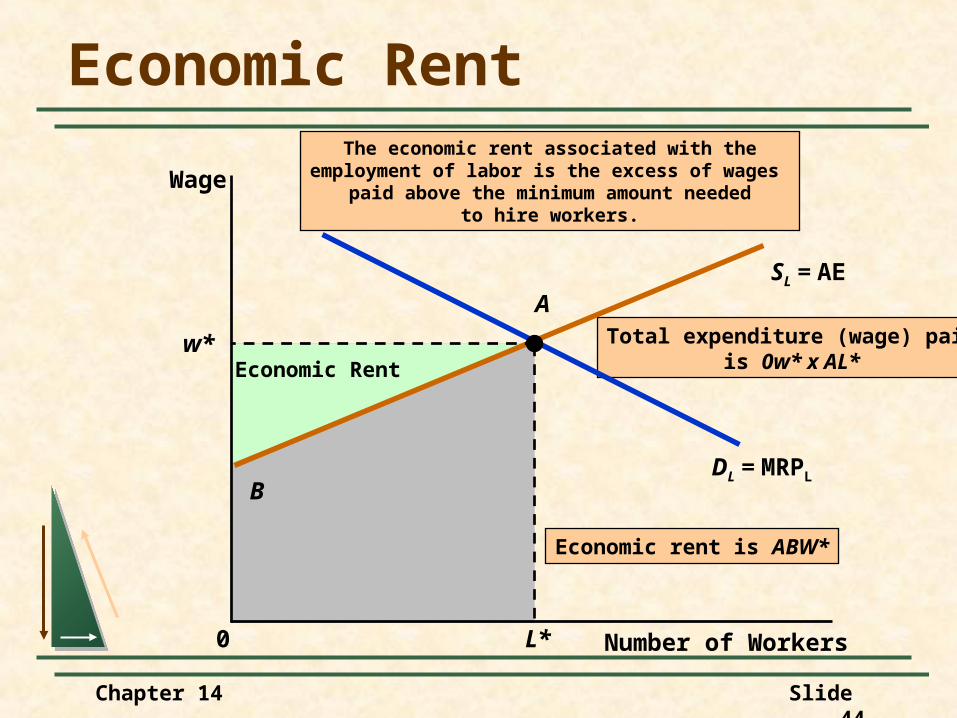
Total expenditure (wage) paidis 0w* x AL*Economic Rent
Economic rent is ABW*
B
Economic Rent
Number of Workers
Wage
SL = AE
DL = MRPL
w*
L*
A
0
The economic rent associated with theemployment of labor is the excess of wages
paid above the minimum amount neededto hire workers.
Chapter 14 Slide 45
Economic Rent
Question
What would be the economic rent if SL is perfectly elastic or perfectly inelastic?
Chapter 14 Slide 46
Land: A Perfectly Inelastic SupplyWith land inelastically supplied, its price is
determined entirely by demand, at least in the short run.
Equilibrium in aCompetitive Factor Market
Chapter 14 Slide 47
EconomicRent
s1
EconomicRent
s2
Land Rent
Number of Acres
Price($ peracre)
Supply of Land
D2
D1

Chapter 14 Slide 48
Pay in the Military
During the Civil War 90% of the armed forces were unskilled workers involved in ground combat.
Today, only 16% are unskilled workers involved in ground combat.

Chapter 14 Slide 49
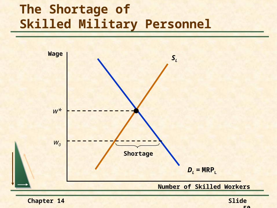
Pay in the Military
Shortages of skilled personnel has occurred? Why?Hint: If there is a shortage, the wage must
be below the…?
Chapter 14 Slide 50
The Shortage ofSkilled Military Personnel
Number of Skilled Workers
WageSL
DL = MRPL
w*
w0
Shortage
Chapter 14 Slide 51
Pay in the Military
Military pay is based on years of service not MRP.
MRP increases and the private sector pay is greater than military pay.
Many leave the military.
Chapter 14 Slide 52
Pay in the Military
SolutionSelective reenlistment bonuses
Base pay on MRP
Chapter 14 Slide 53
Factor Markets with Monopsony Power
AssumeThe output market is perfectly competitive.
Input market is pure monopsony.
Chapter 14 Slide 54
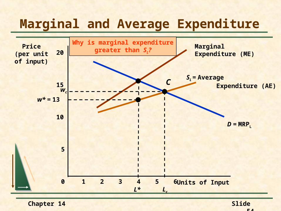
SL = Average Expenditure (AE)
MarginalExpenditure (ME)
Why is marginal expendituregreater than SL?
D = MRPL
Marginal and Average Expenditure
Units of Input
Price(per unitof input)
0 1 2 3 4 65
5
10
15
20
w* = 13
L*
wc
Lc
C
Chapter 14 Slide 55
Factor Markets with Monopsony Power
Examples of Monopsony PowerGovernment
SoldiersMissilesB2 Bombers
NASAAstronauts
Company town
Chapter 14 Slide 56
Monopsony Power inthe Market for Baseball Players
Baseball owners created a monopsonistic cartelReserve clause prevented competition for
players
1975--Free agency after six years
1969--Average salary was $42,000 ($200,000 in 1999 dollars)
1997--Average salary was $1,383,578
Chapter 14 Slide 57
Baseball owners created a monopolistic cartel1975 salaries were 25% of team
expenditures
1980 salaries were 40% of team expenditures
Monopsony Power inthe Market for Baseball Players
Chapter 14 Slide 58
Teenage Labor Marketsand the Minimum Wage
When the minimum wage rose in New Jersey in 1992 from $4.25 to $5.05, a survey conducted found a 13% increase in employment.
Chapter 14 Slide 59
ExplanationsReduction in fringe benefits
Lower pay for more productive workers
Monopsony market
Teenage Labor Marketsand the Minimum Wage
Chapter 14 Slide 60
FindingsNone of the explanations are validated by
the survey results
Indicates of the need for further study
Teenage Labor Marketsand the Minimum Wage
Chapter 14 Slide 61
Factor Markets with Monopoly Power
Just as buyers of inputs can have monopsony power, sellers of inputs can have monopoly power.
The most important example of monopoly power in factor markets involves labor unions.

Chapter 14 Slide 62
SL
DL
MR
When a labor union is a monopolist, it chooses among points on the buyer’s
demand for labor curve.
Monopoly Power of Sellers of Labor
Number of Workers
Wageper
worker
A
L*
w*
The seller can maximize the number of workershired, at L*, by agreeing that workers will
work at wage w*.
Chapter 14 Slide 63
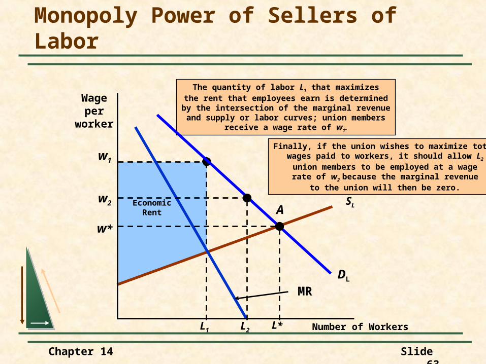
EconomicRent
w1
L1
The quantity of labor L1 that maximizesthe rent that employees earn is determinedby the intersection of the marginal revenueand supply or labor curves; union members
receive a wage rate of w1.
SL
DL
MR
Monopoly Power of Sellers of Labor
Number of Workers
Wageper
worker
A
L2
w2
Finally, if the union wishes to maximize totalwages paid to workers, it should allow L2
union members to be employed at a wagerate of w2 because the marginal revenue
to the union will then be zero.
L*
w*
Chapter 14 Slide 64
The primary determinant of controlling wage and economic rent is controlling the supply of labor
Factor Markets with Monopoly Power
Chapter 14 Slide 65
A Two-Sector Model of Labor EmploymentUnion monopoly power impacts the
nonunionized part of the economy.
Factor Markets with Monopoly Power
Chapter 14 Slide 66
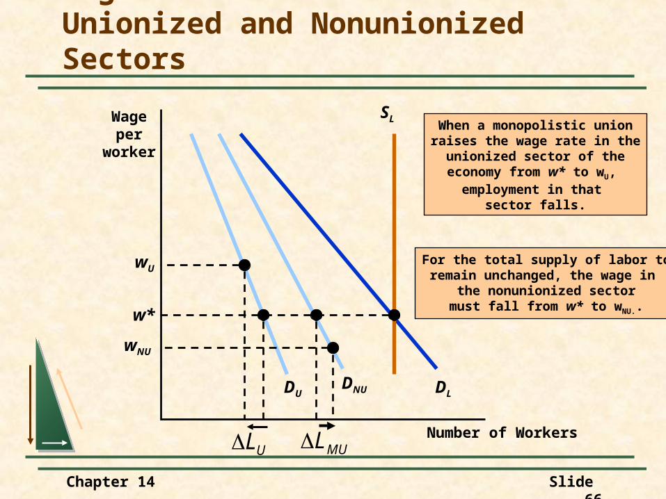
Wage Determination inUnionized and Nonunionized Sectors
Number of Workers
Wageper
worker
DUDNU DL
SL
w*
UL
wU
When a monopolistic unionraises the wage rate in the
unionized sector of theeconomy from w* to wU,
employment in that sector falls.
For the total supply of labor toremain unchanged, the wage in
the nonunionized sectormust fall from w* to wNU..
MUL
wNU
Chapter 14 Slide 67
Bilateral MonopolyMarket in which a monopolist sells to a
monopsonist.
Factor Markets with Monopoly Power
Chapter 14 Slide 68
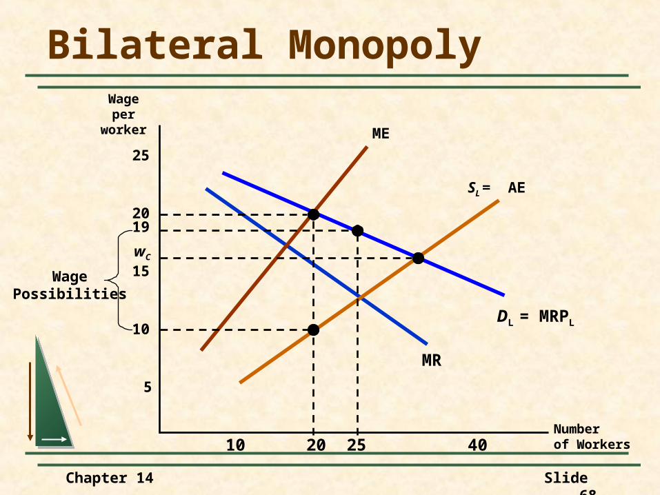
Bilateral Monopoly
Numberof Workers
Wageper
worker
DL = MRPL
MR
5
10
15
20
25
10 20 40
SL = AE
ME
25
19
WagePossibilities
wC
Chapter 14 Slide 69
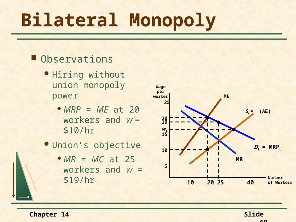
Bilateral Monopoly
Numberof Workers
Wageper
worker
DL = MRPL
MR5
10
15
20
25
10 20 40
SL = (AE)
ME
25
19wC
ObservationsHiring without union
monopoly power MRP = ME at 20
workers and w = $10/hr
Union’s objective MR = MC at 25
workers and w = $19/hr
Chapter 14 Slide 70
Bilateral Monopoly
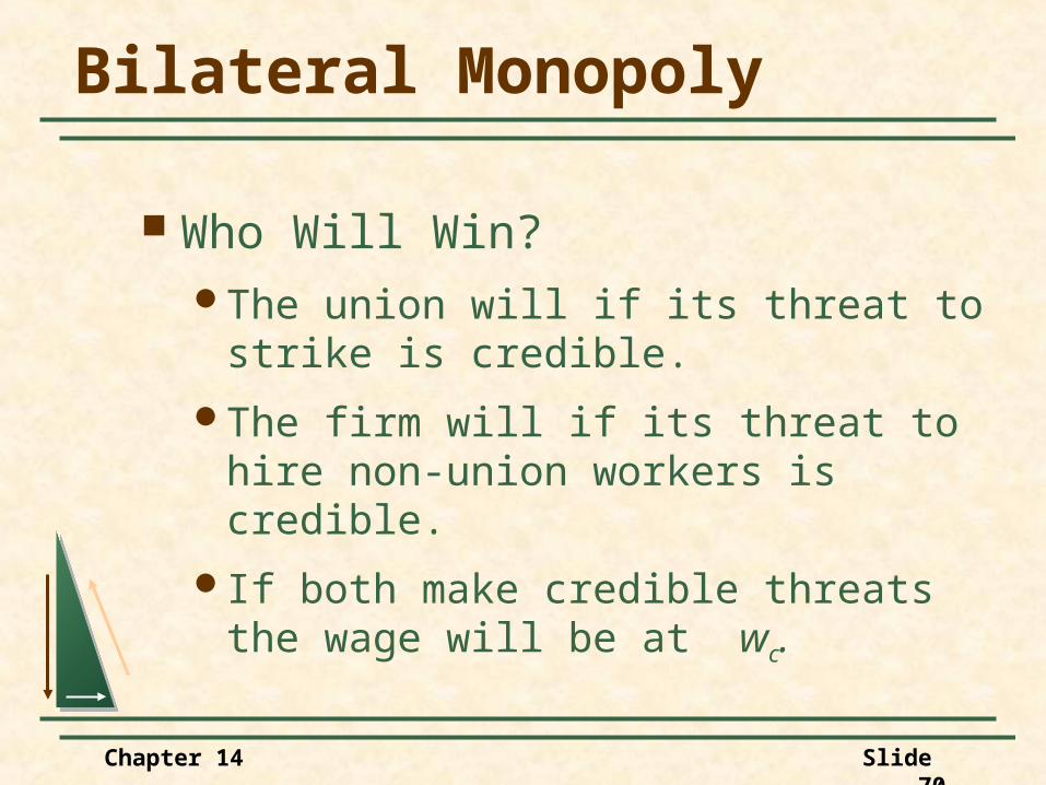
Who Will Win?The union will if its threat to strike is
credible.
The firm will if its threat to hire non-union workers is credible.
If both make credible threats the wage will be at wc.
Chapter 14 Slide 71
The Decline of Private Sector Unionism
ObservationsUnion membership and monopoly power
has been declining.
Initially, during the 1970’s, union wages relative to nonunion wages fell.
Chapter 14 Slide 72
ObservationsIn the 1980’s union wages stabilized
relative to non-union wages.
In the 1990’s membership has been falling and wage differential has remained stable.
The Decline of Private Sector Unionism
Chapter 14 Slide 73
ExplanationThe unions have been attempting to
maximize the individual wage rate instead of total wages paid.
The demand for unionized employees has probably become increasingly elastic as firms find it easier to substitute capital for skilled labor.
The Decline of Private Sector Unionism
Chapter 14 Slide 74
Wage Inequality--HaveComputers Changed the Labor Market?
1950 - 1980Relative wage of college graduates to high-
school graduates hardly changed
1980-1995The relative wage grew rapidly
Chapter 14 Slide 75
Wage Inequality--HaveComputers Changed the Labor Market?
In 1984, 25.1% of all workers used computers
1993 -- 46.6%
1999 -- nearly 60%
Chapter 14 Slide 76
Wage Inequality--HaveComputers Changed the Labor Market?
Percent change in use of computers College degrees
1984 - 1993 -- 42 to 70%
Less than high school degree5 to 10%
With high school degree19 to 35%
Chapter 14 Slide 77
Wage Inequality--HaveComputers Changed the Labor Market?
Growth in wages -- 1983 - 1994College graduates using computers - 11%
Non-computer users -- less than 4%
Chapter 14 Slide 78
Wage Inequality--HaveComputers Changed the Labor Market?
1993 - 1997High school dropouts out of school less
than 10 years earned 29% less than high school graduates
1963 -- The differential was only 19%
Chapter 14 Slide 79
Wage Inequality--HaveComputers Changed the Labor Market?
1993 - 1997Average weekly wage for college
graduates (out of school less than 10 years) was 96% higher than high school graduates.
College graduation premium has more than doubled.
Chapter 14 Slide 80
Summary
In a competitive input market, the demand for an input is given by the MRP, the product of the firm’s marginal revenue, and the marginal product of the input.
A firm in a competitive labor market will hire workers to the point at which the marginal revenue product of labor is equal to the wage rate.
Chapter 14 Slide 81
Summary
The market demand for an input is the horizontal sum of the industry demands for the input.
When factor markets are competitive, the buyer of an input assumes that its purchase will have no effect on the price of the input.
Chapter 14 Slide 82
Summary
The market supply of a factor such as labor need not be upward sloping.
Economic rent is the difference between the payments to factors of production and the minimum payment that would be needed to employ those factors.
Chapter 14 Slide 83
Summary
When a buyer of an input has monopsony power, the marginal expenditure curve lies above the average expenditure curve.
When the input seller is a monopolist such as a labor union, the seller chooses the point on the marginal revenue product curve that best suits its objective.
Chapter 14 Slide 84
Summary
When a monopolistic union bargains with a monopsonistic employer, the wage rate depends on the nature of the bargaining process.
End of Chapter 14
Markets for Factor InputsMarkets for
Factor Inputs