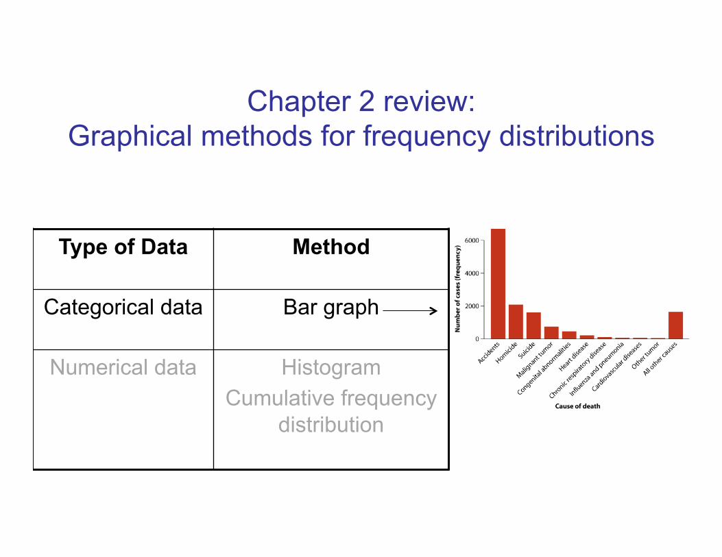
Chapter 2 review: Graphical methods for frequency distributions

Type of Data Method

Categorical data Bar graph

Numerical data Histogram Cumulative frequency

distribution

Chapter 2 review: Graphical methods for frequency distributions

Type of Data Method

Categorical data Bar graph

Numerical data Histogram Cumulative frequency

distribution

Area (thousands of square miles)

Freq

uenc

y

0 5000 10000 15000

010

2030

40

Categorical Numerical

Categorical Contingency table Grouped bar

graph Mosaic plot

Numerical Strip chart Box plot Multiple

histograms

Scatter plot

Chapter 2 review: Graphical methods for associations between

variables

Categorical Numerical

Categorical Contingency table Grouped bar

graph Mosaic plot

Numerical Strip chart Box plot Multiple

histograms

Scatter plot

Chapter 2 review: Graphical methods for associations between

variables

Categorical Numerical

Categorical Contingency table Grouped bar

graph Mosaic plot

Numerical Strip chart Box plot Multiple

histograms

Scatter plot

Chapter 2 review: Graphical methods for associations between

variables

Describing data

Two common descriptions of numerical data

•  Location (or central tendency)

•  Width (or spread)

Measures of location

Mean Median Mode

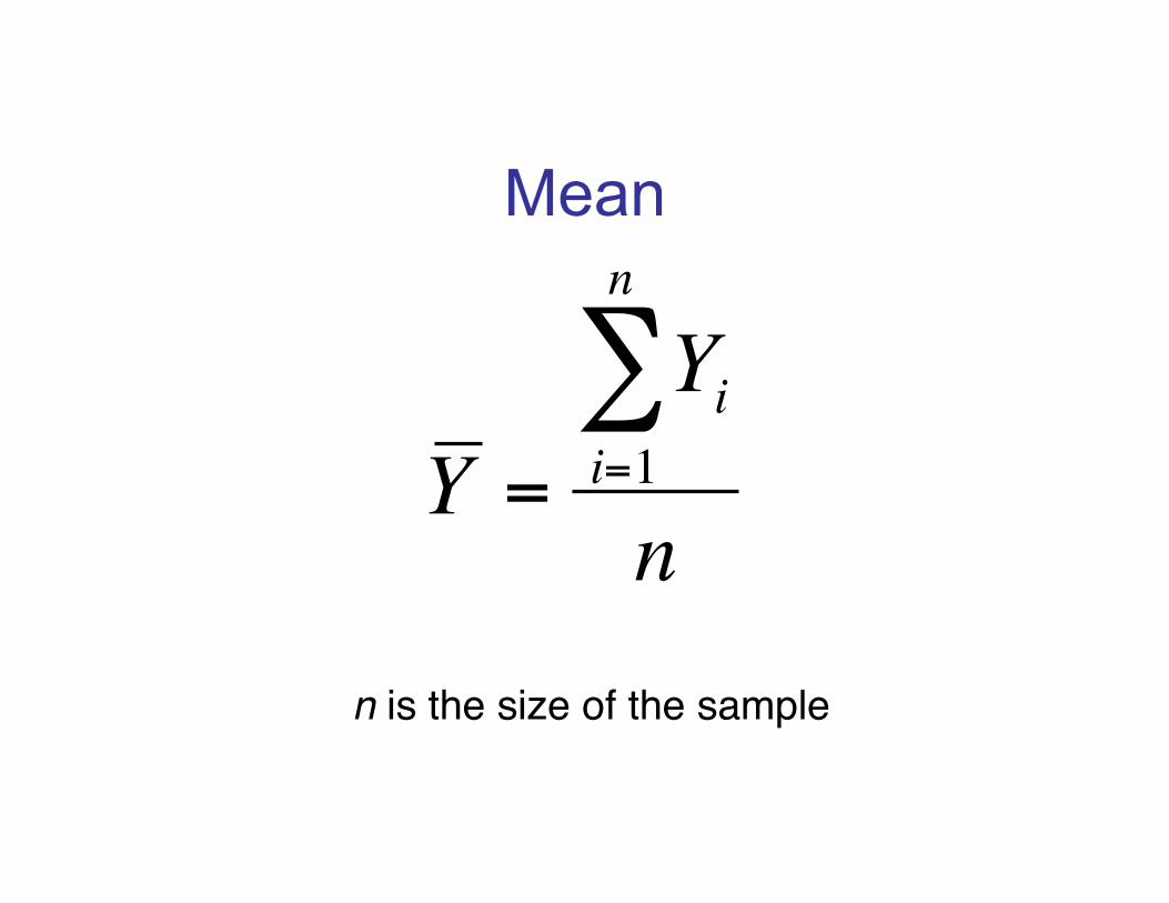
Mean

€

Y =

Yii=1

n

∑n

n is the size of the sample!

Mean

Y1=56, Y2=72, Y3=18, Y4= 42 = (56+72+18+42) / 4 = 47

€

Y

Median

•  The median is the middle measurement in a set of ordered data.

The data: 18 28 24 25 36 14 34 can be put in order: 14 18 24 25 28 34 36 Median is 25

The data: 18 28 24 25 36 14 34 17 can be put in order: 14 17 18 24 25 28 34 36 Median is 24.5

150 160 170 180 190 200 210

0.2

0.4

0.6

0.8

1

Cumulative Frequency

Height (in cm) of Bio300 Students

Mode

The mode is the most frequent measurement.

Genotype Mean Median MM 62.8 63 Mm 50.4 59 mm 11.7 11

How do mean and median compare?

The mean is the center of gravity; "the median is the middle measurement."

The mean is more sensitive to extreme observations than the median"

Mean and median for US household income, 2005

Median $46,326 Mean $63,344 Mode $5000-$9999

Why?"

Mean 169.3 cmMedian 170 cmMode 165-170 cm

University student heights"

Measures of width

•  Range •  Standard deviation •  Variance •  Coefficient of variation •  Interquartile range

Range

14 17 18 20 22 22 24 25 26 28 28 28 30 34 36 The range is the maximum minus the

minimum: 36 -14 = 22

The range is a poor measure of distribution width

Small samples tend to give lower estimates of the range than large samples

So sample range is a biased estimator of the true range of the population."

Variance in a population

€

σ 2 =Yi − µ( )2

i=1

N

∑N

N is the number of individuals in the population."µ is the true mean of the population."

Sample variance

€

s2 =

Yi −Y ( )2i=1

n

∑n −1

n is the sample size!

Example: Sample variance

€

s2 =

Yi −Y ( )2i=1

n

∑n −1

Family sizes of 5 BIOL 300 students: 2 3 3 4 4

€

Y =2 + 3+ 3+ 4 + 4( )

5=165

= 3.22 -1.2 1.44

3 -0.2 0.04

3 -0.2 0.04

4 0.8 0.64

4 0.8 0.64

16 2.80

€

Yi −Y

€

Yi

€

(Yi −Y )2

Sums:"

€

s2 =2.804

= 0.70

“Sum of squares”"

(in units of siblings squared)"

(in units of siblings)"

Shortcut for calculating sample variance

€

s2 =n

n −1# $

% &

Yi2( )

i=1

n

∑n

−Y 2#

$

( ( (

%

&

) ) )

Example: Sample variance (shortcut)

Family sizes of 5 BIOL 300 students: 2 3 3 4 4

€

Y =2 + 3+ 3+ 4 + 4( )

5= 3.2

2 4 -1.2 1.44

3 9 -0.2 0.04

3 9 -0.2 0.04

4 16 0.8 0.64

4 16 0.8 0.64

16 54 2.80

€

Yi −Y

€

Yi

€

(Yi −Y )2

Sums:"

€

s2 =54545− 3.2( )2

#

$ %

&

' ( = 0.70

€

s2 =n

n −1#

$ %

&

' (

Yi2( )

i=1

n

∑n

−Y 2

#

$

% % % %

&

'

( ( ( (

€

Yi2

Standard deviation (SD)

•  Positive square root of the variance

σ is the true standard deviation"s is the sample standard deviation:!

€

s = s2 =

Yi −Y ( )2i=1

n

∑n −1

€

s = 0.70 = 0.84

€

s2 = 0.70

Coefficient of variation (CV)

€

CV = 100% sY

Interquartile Range

Extreme values on box plots

Values lying farther from the box edge than 1.5 times the interquartile range

Skew

•  Skew is a measurement of asymmetry •  Skew (as in "skewer”) refers to the

pointy tail of a distribution

Nomenclature

Population Parameters

Sample Statistics

Mean

Variance s2

Standard Deviation

s €

Y

€

µ

€

σ 2

€

σ

•  Proportion

= number in category n

One common description of categorical data

Brown Blue Hazel Green

Eye Color

Freq

uenc

y

050

100

150

200

p̂

Eye Color Proportion Brown 220 / 592 = 0.37 Blue 215 / 592 = 0.36 Hazel 93 / 592 = 0.16 Green 64 / 592 = 0.11

9 14 4 7 2 18 2

Calculate Mean, Median and Mode

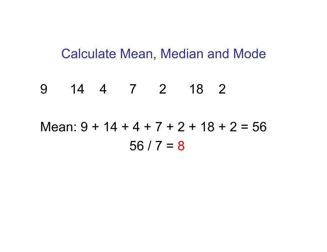
9 14 4 7 2 18 2 Mean: 9 + 14 + 4 + 7 + 2 + 18 + 2 = 56

56 / 7 = 8

Calculate Mean, Median and Mode

9 14 4 7 2 18 2 Mean: 9 + 14 + 4 + 7 + 2 + 18 + 2 = 56

56 / 7 = 8 Median: 2 2 4 7 9 14 18

Calculate Mean, Median and Mode

Calculate Mean, Median and Mode

9 14 4 7 2 18 2 Mean: 9 + 14 + 4 + 7 + 2 + 18 + 2 = 56

56 / 7 = 8 Median: 2 2 4 7 9 14 18 Mode: 2 2 4 7 9 14 18

Calculate Variance and Standard Deviation

9  14 4 7 2 18 2 = 8

€

s2 =

Yi −Y ( )2i=1

n

∑n −1

Variance:" Standard deviation:"

Y

2 -6 36

2 -6 36

4 -4 16

7 -1 1

9 1 1

14 6 36

18 10 100

56 226

€

Yi −Y

€

Yi

€

(Yi −Y )2

Sums:"

= 8"!s2 = 226 / 6 = 37.7""s = " = 6.1 "

Calculate Variance and Standard Deviation

Y

37.7

What are the units?

9  14 4 7 2 18 2 (cm) Mean: 8 cm Median: 7 cm Mode: 2 cm Variance: 37.7 cm2

Standard Deviation: 6.1 cm

Readings

•  We’ve now covered Ch. 1-3

•  Next lecture we’ll cover Ch. 4

Assignment Chapter 1: 14, 17, 19, 20 Chapter 2: 25, 32 Due Friday the 25th by 2 pm in your Ta’s lock box Edition 1 users: Use problems on website! Wrong questions were briefly posted, so if you got them before Tuesday’s class, go back and check that they are the correct ones!