chapter 2 wind resource and site assessment...chapter 2 wind resource and site assessment wiebke...

CHAPTER 2

Wind resource and site assessment

Wiebke Langreder Wind & Site, Suzlon Energy, Århus, Denmark.

Wind farm projects require intensive work prior to the fi nalizing of a project. The wind resource is one of the most important factors for the fi nancial viability of a wind farm project. Wind maps representing the best estimate of the wind resource across a large area have been produced for a wide range of scales, from global down to local government regions. They do not substitute for wind measurements – rather they serve to focus investigations and indicate where on-site measurements would be merited. This chapter explains how wind resource can be assessed. The steps in this process are explained in detail, starting with initial site identifi ca-tion. A range of aspects concerning wind speed measurements is then covered including the choice of sensors, explaining the importance of proper mounting and calibration, long-term corrections, and data analysis. The diffi culty of extrapolat-ing the measured wind speed vertically and horizontally is demonstrated, leading to the need for fl ow models and their proper use. Basic rules for developing a layout are explained. Having analysed wind data and prepared a layout, the next step is energy yield calculation.The chapter ends by exploring various aspects of site suitability.

1 Initial site identifi cation

The wind resource is one of the most critical aspects to be assessed when plan-ning a wind farm. Different approaches on how to obtain information on the wind climate are possible. In most countries where wind energy is used extensively, some form of general information about the wind is available. This information could consist of wind maps showing colour coded wind speed or energy at a spe-cifi c height. These are often based on meso-scale models and in the ideal case, are validated with ground-based stations. The quality of these maps varies widely and depends on the amount and precision of information that the model has been fed with, the validation process and the resolution of the model.

www.witpress.com, ISSN 1755-8336 (on-line) WIT Transactions on State of the Art in Science and Engineering, Vol 44, © 2010 WIT Press

doi:10.2495/978-1-84564- /205-1 02

50 Wind Power Generation and Wind Turbine Design

Wind atlases are normally produced with Wind Atlas Analysis and Application Program (WAsP, a micro-scale model, see Section 4.3) or combined models which involve the use of both meso- and micro-scale models, and are presented as a col-lection of wind statistics. The usefulness of these wind statistics depends very much on the distance between the target site and the stations, the input data they are based on, the site as well as on the complexity of the area, both regarding roughness and orography. Typically the main source of information for wind atlases is meteorological stations with measurements performed at a height of 10 m. Meso-scale models additionally use re-analysis data (see Section 3.1.1). Care has to be taken since the main purpose of these data is to deliver a basis for general weather models, which have a much smaller need for high precision wind measurements than wind energy. Thus the quality of wind atlases is not suffi cient to replace on-site measurements [ 1 ].

Nature itself frequently gives reasonable indications of wind resources. Particu-larly fl agged trees and bushes can indicate a promising wind climate and can give valuable information on the prevailing wind direction.

A very good source of information for a fi rst estimate of the wind regime is production data from nearby wind farms, if available.

No other step in the process of wind farm development has such signifi cance to the fi nancial success as the correct assessment of the wind regime at the future turbine location. Because of the cubic relationship between wind speed and energy content in the wind, the prediction of energy output is extremely sensitive to the wind speed and requires every possible attention.

2 Wind speed measurements

2.1 Introduction

The measured wind climate is the main input for the fl ow models, by which you extrapolate the spot measurement vertically and horizontally to evaluate the energy distribution across the site. Such a resource map is the basis for an optimised lay-out. The number and height of the measurement masts should be adjusted to the complexity of the terrain as with increasing complexity, the capability of fl ow models to correctly predict the spatial variation of the wind decreases. The more complex the site, the more and the higher masts have to be installed to ensure a reasonable prediction of the wind resource.

Unfortunately wind measurements are frequently neglected. Very often the measurement height is insuffi cient for the complexity of the site, the number of masts is insuffi cient for the size of the site, the measurement period is too short, the instruments are not calibrated, the mounting is sub-standard or the mast is not maintained. It cannot be stressed enough that the most expensive part when measuring wind is the loss of data. Any wind resource assessment requires a minimum measurement period of one complete year in order to avoid seasonal biases. If instrumentation fails due to lightning strike, icing, vandalism or other reasons and the failure is not spotted rapidly, the lost data


Wind Resource and Site Assessment 51

will falsify the results and as a consequence the measurement period has to start all over again. Otherwise the increased uncertainty might jeopardise the feasibility of the whole project.

2.2 Instruments

2.2.1 General Wind speed measurements put a very high demand on the instrumentation because the energy density is proportional to the cube of the mean wind speed. Further-more, the instruments used must be robust and reliably accumulate data over extended periods of unattended operation. The power consumption should be low so that they can operate off the grid.

Most on-site wind measurements are carried out using the traditional cup ane-mometer. The behaviour of these instruments is fairly well understood and the sources of error are well known. In general, the sources of error in anemometry include the effects of the tower, boom and other mounting arrangements, the ane-mometer design and its response to turbulent and non-horizontal fl ow characteris-tics, and the calibration procedure. Evidently, proper maintenance of the anemometer is also important. In some cases, problems arise due to icing of the sensor, or corrosion of the anemometer at sites close to the sea. The current version of the internationally used standard for power curve measurements, the IEC stan-dard 61400-12-1 [ 2 ], only permits the use of cup anemometry for power curve measurements. The same requirements for accuracy are valid for wind resource measurements. Therefore it is advisable to use also these instruments for wind resource assessment.

Solid state wind sensors (e.g. sonics) have until recently not been used exten-sively for wind energy purposes, mainly because of their high cost and a higher power consumption. These have a number of advantages over mechanical ane-mometers and can further provide measurements of turbulence, air temperature, and atmospheric stability. However, they also introduce new sources of error which are less known, and the overall accuracy of sonic anemometry is lower than for high-quality cup anemometry [ 3 ].

Recently, remote sensing devices based either on sound (Sodar) or on laser (Lidar) have made an entry into the market. Their clear merit is that they replace a mast which can have practical advantages. However, they often require more substantial power supplies which bring other reliability and deployment issues. Also more intensive maintenance is required since the mean time between failures does not allow unattended measurements for peri-ods required for wind resource assessment. While the precision of a Lidar seems to be superior to the Sodar, and often comparable to cup anemometry [ 4 ], both instruments suffer at the moment from short-comings in complex ter-rain due to the fact that the wind speed sampling takes place over a volume, and not at a point.

Remote sensing technologies are currently evolving very rapidly and it is expected they will have a signifi cant role to play in the future.



2.2.2 Cup anemometer The cup anemometer is a drag device and consists typically of three cups each mounted on one end of a horizontal arm, which in turn are mounted at equal angles to each other on a vertical shaft. A cup anemometer turns in the wind because the drag coeffi cient of the open face cup is greater than the drag coeffi cient of the smooth surface of the back. The air fl ow past the cups in any horizontal direction turns the cups in a manner that is proportional to the wind speed. Therefore, count-ing the turns of the cups over a set time period produces the average wind speed for a wide range of speeds.

Despite the simple geometry of an anemometer its measurement behaviour depends on a number of different factors. One of the most dominant factors is the so-called angular response, which describes what components of the wind vector are measured [ 3 ]. A so-called vector anemometer measures all three components of the wind vector, the longitudinal, lateral and vertical component. Thus this type of ane-mometer measures independently of the infl ow angle and is less sensitive to mount-ing errors, terrain inclination and/or thermal effects. However, for power curve measurements the instrument must have a cosine response thus measuring only the horizontal component of the wind [ 2 ]. Since for energy yield calculations the mea-surement behaviour of the anemometer used for the power curve and used for resource assessment should be as similar as possible, it is advisable to also use an anemometer with a cosine response for resource assessment. One of the key argu-ments for using such an instrument for power curve measurements is that the wind turbine utilises only the horizontal component. This is, however, a very simplifi ed approach as, particularly for large rotors, three-dimensional effects along the blades leads to a utilisation of energy from the vertical component. Care has to be taken when using a cosine response anemometer as it is sensitive to mounting errors.

One of the most relevant dynamic response specifi cations is the so-called over-speeding. Due mainly to the aerodynamic characteristics of the cups, the anemom-eter tends to accelerate faster than it decelerates, leading to an over-estimate of wind speed particularly in the middle wind speed range.

Another dynamic response specifi cation is the response length or distance con-stant, which is related to the inertia of the cup anemometer. The dynamic response can be described as a fi rst order equation. When a step change of wind speed from U to U + Δ u hits the anemometer it will react with some delay of exponential shape. The distance constant, i.e. the column of air corresponding to 63% recovery time for a step change in wind speed, should preferably be a few meters or less. Different methods to determine the response length are described in [ 3 ].

2.2.3 Ultrasonic anemometer Ultrasonic or sonic anemometers use ultrasonic waves for measuring wind speed and, depending on the geometry, the wind direction. They measure the wind speed based on the time of fl ight between pairs of transducers. Depending on the num-ber of pairs of transducers, either one-, two- or three-dimensional fl ow can be measured. The travelling time forth and back between the transducers is different because in one direction the wind speed component along the path is added to the



sound speed and subtracted from the other direction. If the distance of the trans-ducers is given with s and the velocity of sound with c then the travelling times can be expressed as

1 2and

s st t

c u c u= =

+ − (1)

These equations can be re-arranged to eliminate c and to express the wind speed u as a function of t 1 , t 2 and s . The sole dependency on the path length is advanta-geous, as the speed of sound depends on air density and humidity:

1 2

1 1

2

su

t t

⎛ ⎞= −⎜ ⎟⎝ ⎠

(2)

It can be seen that once u is known, c can be calculated and from c the tempera-ture can be inferred (slightly contaminated with humidity, this is known as the “sound virtual temperature”). The spatial resolution is determined by the path length between the transducers, which is typically 10–20 cm. Due to the very fi ne temporal resolution of 20 Hz or better the sonic anemometer is very well suited for measurements of turbulence with much better temporal and spatial resolution than cup anemometry.

The measurement of different components of the wind, the lack of moving parts, and the high temporal resolutions make the ultrasonic anemometer a very attrac-tive wind speed measurement device. The major concern, inherent in sonic ane-mometry, is the fact that the probe head itself distorts the fl ow – the effect of which can only be evaluated in detail by a comprehensive wind tunnel investigation. The transducer shadow effect is a particularly simple case of fl ow distortion and a well-known source of error in sonics with horizontal sound paths. Less well known are the errors associated with inaccuracies in probe head geometry and the tempera-ture sensitivity of the sound transducers. The measurement is very sensitive to small variations in the geometry, either due to temperature variations and/or mechanical vibrations due to wind. Finally, specifi c details in the design of a given probe head may give rise to wind speed-dependent errors.

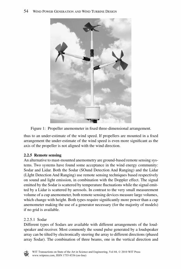
2.2.4 Propeller anemometer A propeller anemometer typically has four helicoid-shaped blades. This propeller can either be mounted in conjunction with a wind vane or in a fi xed two- or three-dimensional arrangement ( Fig. 1 ). While a cup anemometer responds to the dif-ferential drag force, both drag and lift forces act to turn the propeller anemometer. Similar to a cup anemometer the response of the propeller anemometer to slow speed variations is linear above the starting threshold.

Propeller anemometers have an angular response that deviates from cosine. In fact the wind speed measured is somewhat less than the horizontal component [ 5 ]. If a propeller is used in conjunction with a vane the propeller is in theory on average oriented into the wind and thus the angular response is not so relevant. However, the vane often shows an over-critical damping which leads to misalignment and



thus to an under-estimate of the wind speed. If propellers are mounted in a fi xed arrangement the under-estimate of the wind speed is even more signifi cant as the axis of the propeller is not aligned with the wind direction.

2.2.5 Remote sensing An alternative to mast-mounted anemometry are ground-based remote sensing sys-tems. Two systems have found some acceptance in the wind energy community: Sodar and Lidar. Both the Sodar (SOund Detection And Ranging) and the Lidar (LIght Detection And Ranging) use remote sensing techniques based respectively on sound and light emission, in combination with the Doppler effect. The signal emitted by the Sodar is scattered by temperature fl uctuations while the signal emit-ted by a Lidar is scattered by aerosols. In contrast to the very small measurement volume of a cup anemometer, both remote sensing devices measure large volumes, which change with height. Both types require signifi cantly more power than a cup anemometer making the use of a generator necessary (for the majority of models) if no grid is available.

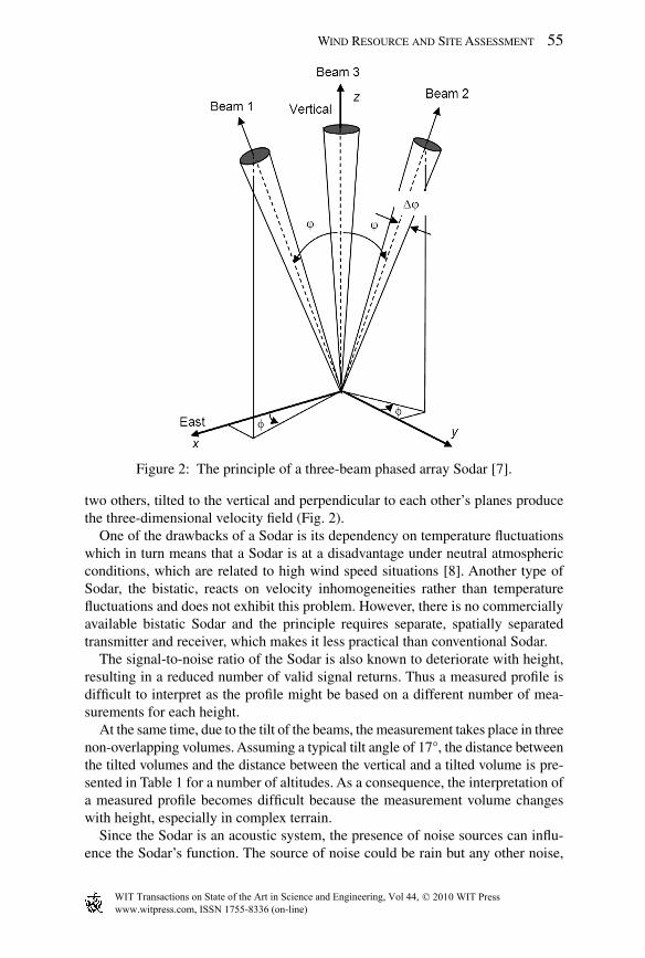
2.2.5.1 Sodar Different types of Sodars are available with different arrangements of the loud-speaker and receiver. Most commonly the sound pulse generated by a loudspeaker array can be tilted by electronically steering the array to different directions (phased array Sodar). The combination of three beams, one in the vertical direction and

Figure 1: Propeller anemometer in fi xed three-dimensional arrangement .



two others, tilted to the vertical and perpendicular to each other’s planes produce the three-dimensional velocity fi eld ( Fig. 2 ).

One of the drawbacks of a Sodar is its dependency on temperature fl uctuations which in turn means that a Sodar is at a disadvantage under neutral atmospheric conditions, which are related to high wind speed situations [ 8 ]. Another type of Sodar, the bistatic, reacts on velocity inhomogeneities rather than temperature fl uctuations and does not exhibit this problem. However, there is no commercially available bistatic Sodar and the principle requires separate, spatially separated transmitter and receiver, which makes it less practical than conventional Sodar.

The signal-to-noise ratio of the Sodar is also known to deteriorate with height, resulting in a reduced number of valid signal returns. Thus a measured profi le is diffi cult to interpret as the profi le might be based on a different number of mea-surements for each height.

At the same time, due to the tilt of the beams, the measurement takes place in three non-overlapping volumes. Assuming a typical tilt angle of 17°, the distance between the tilted volumes and the distance between the vertical and a tilted volume is pre-sented in Table 1 for a number of altitudes. As a consequence, the interpretation of a measured profi le becomes diffi cult because the measurement volume changes with height, especially in complex terrain.

Since the Sodar is an acoustic system, the presence of noise sources can infl u-ence the Sodar’s function. The source of noise could be rain but any other noise,

Figure 2: The principle of a three-beam phased array Sodar [ 7 ] .



for example from animals, can have an adverse effect. A particularly critical issue is the increased background noise due to high wind speeds [ 9 ]. False echoes from the Sodar’s enclosure or nearby obstacles can also lead to a falsifi ed signal. Other parameters which may infl uence the Sodar measurement are errors in the vertical alignment of the instrument, temperature changes at the antenna and, especially for three-beam Sodars, changes in wind direction [ 8 ].

The measurement accuracy of Sodar systems cannot match that of cup ane-mometry and unless high acoustical powers are used, their availability falls in high wind speeds. A hybrid system comprising a moderately tall mast (say 40 m) and a relatively low power (30–100 W electrical) Sodar has many attractive features – the high absolute accuracy and high availability of the cup anemom-eter complements the less accurate but highly relevant vertical resolution obtained from the Sodar [ 10 ].

2.2.5.2. Lidar Until recently, making wind measurements using Lidars was prohibitively expensive and essentially limited to the aerospace and military domain. Most limitations were swept aside by the emergence of coherent lasers at wave-lengths compliant with fi bre optic components (so-called ‘fi bre lasers’). Since light can be much more precisely focused and spreads in the atmosphere much less than sound, Lidar systems have an inherently higher accuracy and better signal to noise ratio than a Sodar. The Lidar works by focusing at a specifi c distance and it measures the scattering from aerosols that takes place within the focal volume.

The operation of the Lidar is infl uenced by atmospheric conditions (e.g. fog, density of particles in the air). Lack of particles infl uences its response, some-times prohibiting measurement while fog can severely attenuate the beam before it reaches the measurement height. Rain also reduces the Lidar’s ability to measure, as scattering from the falling droplets can result in errors in the wind speed, particularly its vertical components. Other parameters that infl u-ence the measurement are, as in the case of the Sodar: errors in the vertical alignment of the instrument and uncertainties in the focusing height. The Lidar,

Table 1: The distance between the three beams at a number of heights [ 9 ].

Altitude (m)

Distance (m)

Tilt–vertical Tilt–tilt

40 11.7 16.580 23.4 33.1120 35.1 49.6160 46.8 66.2200 58.5 82.7



being an optical instrument, is also susceptible to infl uences from the presence of dirt on the output window; hence there is a need for a robust cleaning device of the Lidar window [ 9 ].

Two working principles of fi bre-base Lidars are in use: one uses a continu-ous-wave system with height discrimination achieved by varying focus. The laser light is emitted through a constantly rotating prism giving a defl ection of 30° from the vertical. This Lidar system scans a laser beam about a vertical axis from the ground, intercepting the wind on a 360° circumference. By adjusting the laser focus, winds may be sampled at a range of heights above ground level.

The other system uses a pulsed signal with a fi xed focus. It has a 30° prism to defl ect the beam from the vertical but here the prism does not rotate continuously. Instead, the prism remains stationary whilst the Lidar sends a stream of pulses in a given direction, recording the backscatter in a number of range gates (fi xed time delays) triggered by the end of each pulse [ 10 ] (see Fig. 3 ).

Unlike pulsed systems, continuous-wave Lidar systems do not inherently ‘know’ the height from which backscatter is being received. A sensibly uniform vertical profi le of aerosol concentration has to be assumed in which case the backscattered energy is from the focused volume. The obtained radial wind speed distribution in this case is dominated by the signal from the set focus distance. The assumption of vertical aerosol homogeneity unfortunately fails completely in the fairly common case of low level clouds (under 1500 m). Here, the relatively huge backscatter from the cloud base can be detected even though the cloud is far above the focus distance. The resulting Doppler spectrum has two peaks – one corresponding to the radial speed at the focused height and a second corresponding to the (usually) higher speed of the cloud base. Unless corrected for, this will introduce a bias to the wind speed measurement. For this reason, the continuous-wave Lidar has a cloud-correction algorithm that identifi es the second peak and rejects it from the

Figure 3: Working principle of a pulsed Lidar .



spectrum. An extra second scan with a near-collimated output beam is inserted into the height cycle. The spectra thus measured are used to remove the infl uence of the clouds at the desired measuring heights [ 10 ].

The two systems have fundamental differences concerning the measurement volume. The continuous-wave system adjusts the focus so winds may be sam-pled at a range of heights above ground level. The backscattered signal comes mainly from the region close to the beam focus, where the signal intensity is at its maximum. While the width of the laser beam increases in proportion to focus height, its probe length increases non-linearly (roughly the square of height; Table 2 ). The vertical measuring depth of the pulsed system depends on the pulse length and is constant with sensing range [ 10 ]. A continuous-wave system can measure wind speed at heights from less than 10 m up to a maximum of about 200 m. Pulsed Lidars are typically blinded during emission of the pulse and this restricts their minimum range to about 40 m, with the maximum range usually limited only by signal-to-noise considerations and hence dependent on conditions.

Like the Sodar, both Lidar systems rely on the assumption of horizontally homo-geneous fl ow. In complex terrain this assumption is violated, increasingly so as the terrain complexity increases. There are indications that errors of 5–10% in the mean speed are not uncommon [12–14]. Only a multiple Lidar system, in which units are separated along a suitably long baseline, could eliminate this inherent error as explained above.

In general, care has to be taken when performing short-term measurements with remote sensing devices. The vertical profi le varies signifi cantly with different atmospheric stabilities. Thus the measurement campaign using remote sensing should, similarly to cup anemometry, be a minimum of 1 year.

Currently work is in progress for a Best Practice Guideline for the use of remote sensing.

2.3 Calibration

As explained in Section 2.2.2, the turns of an anemometer are transformed into a wind speed measurement by a linear function. The scale and offset of this trans-fer function are determined by wind tunnel calibration of the anemometer. Strict requirements concerning the wind tunnel test are specifi ed in [ 2 ]. Please note that

Table 2: Beam half-length versus focal distance of a continuous-wave Lidar [ 11 ].

Altitude (m) Beam half-length, L (m)

40 2.5 60 6100 16200 65



such strict calibration procedures are only in place for cup anemometers. Highest quality calibrations are ensured when calibrating in wind tunnels that have been accredited by MEASNET. MEASNET members participate regularly in a round robin test to guarantee interchangeability of the results, which has increased the quality of the calibration signifi cantly. It should be kept in mind that even calibrations according to highest standard bear an uncertainty of around 1–2%.

Currently there are no calibration standards available for sonics and remote sensing devices.

2.4 Mounting

Accurate wind speed measurements are only possible with appropriate mounting of the cup anemometry on the meteorological mast. In particular, the anemometer shall be located such that the fl ow distortion due to the mast and the side booms is minimised. The least fl ow distortion is found by mounting the anemometer on top of the mast at a suffi cient distance to the structure. Other instruments, aviation lighting, and the lightning protection should be mounted in such a way that interference with the anemometer is avoided. Figure 4 shows a possible top mounting arrangement.

Boom-mounted anemometers are infl uenced by fl ow distortion of both the mast and the boom. Flow distortion due to the mounting boom should be kept below 0.5% and fl ow distortion due to the mast should be kept below 1%. If the anemom-eter is mounted on a tubular side boom, this can be achieved by mounting the anemometer 15 times the boom diameter above the boom. The level of fl ow distor-tion due the mast depends on the type of mast and the direction the anemometer is facing with respect to the mast geometry and the main wind direction.

Figure 4: Example top mounted anemometers [ 2 ].



Figure 5 shows an example of fl ow distortion around a tubular mast. It can be seen that there is a deceleration of the fl ow upwind to the mast, acceleration around it and a wake behind it. The least disturbance can be seen to occur if facing the wind at 45°.

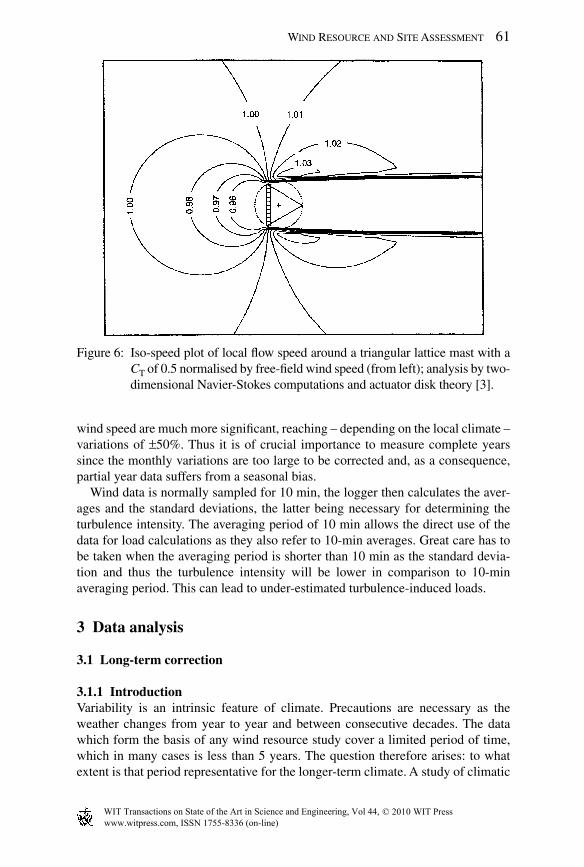
The fl ow distortion around a lattice mast is somewhat more complicated to determine. Additionally to the orientation of the wind and the distance of the ane-mometer to the centre of the mast it also depends on the solidity of the mast and the drag. Figure 6 shows an example of fl ow distortion. Again a deceleration in front of the mast can be observed while there is acceleration at the fl anks. Mini-mum distortion is achieved when the anemometer is placed at an angle of 60°. More details on how to determine the fl ow distortion can be found in [ 3 ] or [ 2 ].

In general, mounting of the anemometer at the same height as the top of the mast should be avoided since the fl ow distortion around the top of the mast is highly complex and cannot be corrected for.

2.5 Measurement period and averaging time

The energy yield is typically calculated referring to the annual mean wind speed of the site. Unfortunately the annual average wind speed varies signifi cantly. Depending on the local climate the annual averages of wind speed might vary around ± 15% from one year to the next. To reduce the uncertainty of the inter-annual variability it is strongly recommended to perform a long-term correction of the measured data (see Section 3.1). On a monthly scale, the variations of the

Figure 5: Iso-speed plot of local fl ow speed around a cylindrical mast, norma-lised by free-fi eld wind speed (from left); analysis by two-dimensional Navier-Stokes computations [ 3 ].



wind speed are much more signifi cant, reaching – depending on the local climate – variations of ± 50%. Thus it is of crucial importance to measure complete years since the monthly variations are too large to be corrected and, as a consequence, partial year data suffers from a seasonal bias.

Wind data is normally sampled for 10 min, the logger then calculates the aver-ages and the standard deviations, the latter being necessary for determining the turbulence intensity. The averaging period of 10 min allows the direct use of the data for load calculations as they also refer to 10-min averages. Great care has to be taken when the averaging period is shorter than 10 min as the standard devia-tion and thus the turbulence intensity will be lower in comparison to 10-min averaging period. This can lead to under-estimated turbulence-induced loads.

3 Data analysis

3.1 Long-term correction

3.1.1 Introduction Variability is an intrinsic feature of climate. Precautions are necessary as the weather changes from year to year and between consecutive decades. The data which form the basis of any wind resource study cover a limited period of time, which in many cases is less than 5 years. The question therefore arises: to what extent is that period representative for the longer-term climate. A study of climatic

Figure 6: Iso-speed plot of local fl ow speed around a triangular lattice mast with a C T of 0.5 normalised by free-fi eld wind speed (from left); analysis by two-dimensional Navier-Stokes computations and actuator disk theory [ 3 ].



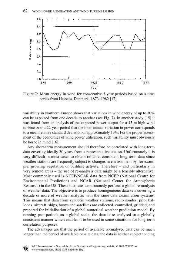
variability in Northern Europe shows that variations in wind energy of up to 30% can be expected from one decade to another (see Fig. 7 ). In another study [ 15 ] it was found from an analysis of the expected power output for a 45 m high wind turbine over a 22-year period that the inter-annual variation in power corresponds to a mean relative standard deviation of approximately 13%. For the proper assess-ment of the economics of wind power utilisation, such variability must obviously be borne in mind [ 16 ].

Any short-term measurement should therefore be correlated with long-term data covering ideally 30 years from a representative station. Unfortunately it is very diffi cult in most cases to obtain reliable, consistent long-term data since weather stations are frequently subject to changes in environment by, for exam-ple, growing vegetation or building activity. Therefore – and particularly in very remote areas – the use of re-analysis data might be a feasible alternative. Most commonly used is NCEP/NCAR data from NCEP (National Centre for Environmental Prediction) and NCAR (National Center for Atmospheric Research) in the US. These institutes continuously perform a global re-analysis of weather data. The objective is to produce homogeneous data sets covering a decade or more of weather analysis with the same data assimilation systems. This means that data from synoptic weather stations, radio sondes, pilot bal-loons, aircraft, ships, buoys and satellites are collected, controlled, gridded, and prepared for initialisation of a global numerical weather prediction model. By running past-periods on a global scale, the data is re-analysed in a globally consistent manner which enables it to be used in some situations for long-term correlation purposes.

The advantages are that the period of available re-analysed data can be much longer than the period of available on-site data, the data is neither subject to icing

Figure 7: Mean energy in wind for consecutive 5-year periods based on a time series from Hesselø, Denmark, 1873–1982 [ 17 ] .



nor seasonal infl uences from vegetation and fi nally there should be no long-term equipment trends. However the quality of re-analysis data still depends on the quality of the input data, with the result that in sparsely instrumented regions, the re-analysis data can still suffer from defi ciencies in individual instrumentation and data coverage. The same care should be applied to the use of re-analysis data, as with ground-based data. The NCEP/NCAR data is available in the form of pres-sure and surface wind data in a 2.5° grid corresponding to a spacing of approxi-mately 250 km. The data consists of values of wind speed and direction for four instantaneous values per day (every 6 hours).

The statistical method for long-term correcting data is called Measure-Correlate-Predict or MCP. This method is based on the assumption that the short- and long-term data sets are correlated. This correlation can be established in different ways depending on the data quality and the comparability of the two wind climates.

3.1.2 Regression method If one mast is correlated with a second on-site mast, a linear regression either omnidirectional or by wind direction sectors (typically 30°) might be best suited. For the concurrent period, the wind speeds are plotted versus each other and a linear regression based on the least-square fi t is established. This relationship is used to extend the shorter data set with synthetic data based on the longer data set. The regression coeffi cient is a measure of the quality of the correlation. R 2 should not be less than 70%. The same method might be appropriate for a short-term measurement on-site and a reference station in some distance if the orography and the wind roses are closely related. If the wind roses vary, care has to be taken since the wind rose of the reference station will be transferred to the site by applying a linear regression, which can have a signifi cant impact on the layout as well as the energy yield. Another inherent problem of this methodol-ogy is the decreasing temporal correlation between the site and the reference station with increasing distance. The introduction of averaging of the two data sets can improve the correlation.

3.1.3 Energy index method Rather than transposing the wind distribution from the reference station the energy index method determines a correction factor for the short-term data. For the con-current period, the energy level of the reference data set is determined and com-pared with the long-term energy. The resulting ratio is then applied as correction to the short-term on-site data set. The correlation is best proven comparing monthly mean wind speeds of the two data sets.

This method has the main advantage that the on-site measured wind rose is not altered. The energy index method is particularly suited for NCEP/NCAR data since the low temporal resolution of NCEP/NCAR prohibits the use of the more detailed regression method. However, care has to be taken since NCEP/NCAR data represents only geostrophic wind and does not refl ect local wind climates like wind tunnel effects across a mountain pass or thermal effects.



3.2 Weibull distribution

It is very important for the wind industry to be able to relatively simply describe the wind regime on site. Turbine designers need the information to optimise the design of their turbines, so as to minimise generating costs. Turbine investors need the information to estimate their income from electricity generation.

One way to condense the information of a measured time series is a histogram. The wind speeds are sorted into wind speed bins. The bin width is typically 1 m/s. The histogram provides information how often the wind is blowing for each wind speed bin.

The histogram for a typical site can be presented using the Weibull distribution expressing the frequency distribution of the wind speed in a compact form. The two-parameter Weibull distribution is described mathematically as

− ⎛ ⎞⎛ ⎞ ⎛ ⎞= −⎜ ⎟⎜ ⎟ ⎜ ⎟⎝ ⎠ ⎝ ⎠⎝ ⎠

1

( ) expk k

k u uf u

A A A (3)

where f ( u ) is the frequency of occurrence of wind speed u . The scaling factor A is a measure for the wind speed while the shape factor k describes the shape of the distribution. The cumulative Weibull distribution F ( u ) gives the probability of the wind speed exceeding the value v and is given by the simple expression:

( ) expk

uF u

A

⎛ ⎞⎛ ⎞= −⎜ ⎟⎜ ⎟⎝ ⎠⎝ ⎠ (4)

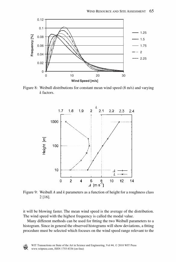
Following graph shows a group of Weibull distributions with a constant mean wind speed of 8 m/s but varying k factor. Note that high wind speeds become more probable with a low k factor.

The Weibull distribution can degenerate into two special distributions, namely for k = 1 the exponential distribution and k = 2 the Rayleigh distribution. Since observed wind data exhibits frequency distributions which are often well described by a Rayleigh distribution, this one-parameter distribution is sometimes used by wind turbine manufacturers for calculation of standard performance fi gures for their machines. Inspection of the k parameter shows that, especially for Northern European climates, the values for k are indeed close to 2.0.

On a global scale, the k factor varies signifi cantly depending upon local climate conditions, the landscape, and its surface ( Fig. 8 ). A low k factor (<1.8) is typical for wind climates with a high content of thermal winds. A high k factor (>2.5) is representative for very constant wind climates, for example trade winds. Both Weibull A and k parameters are dependent on the height and are increasing up to 100 m above ground ( Fig. 9 ). Above 100 m the k parameter decreases.

The Weibull distribution is a probability density distribution. The median of the distribution corresponds to the wind speed that cuts the area into half. This means that half the time it will be blowing less than the median wind speed, the other half



it will be blowing faster. The mean wind speed is the average of the distribution. The wind speed with the highest frequency is called the modal value.

Many different methods can be used for fi tting the two Weibull parameters to a histogram. Since in general the observed histograms will show deviations, a fi tting procedure must be selected which focuses on the wind speed range relevant to the

0

0.02

0.04

0.06

0.08

0.1

0.12

0 10 20 30

Fre

qu

ency

[%

]

Wind Speed [m/s]

1.25

1.5

1.75

2

2.25

Figure 8: Weibull distributions for constant mean wind speed (8 m/s) and varying k factors .

Figure 9: Weibull A and k parameters as a function of height for a roughness class 2 [ 16 ] .



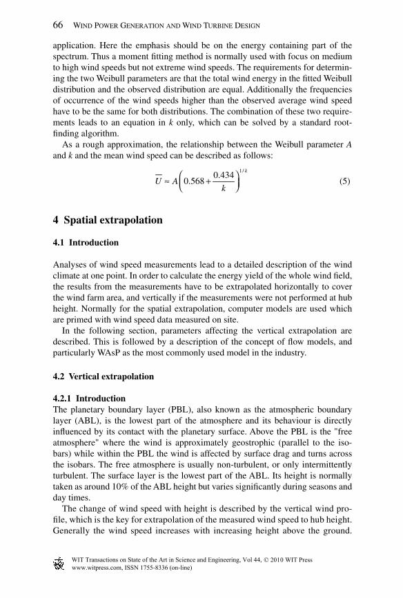
application. Here the emphasis should be on the energy containing part of the spectrum. Thus a moment fi tting method is normally used with focus on medium to high wind speeds but not extreme wind speeds. The requirements for determin-ing the two Weibull parameters are that the total wind energy in the fi tted Weibull distribution and the observed distribution are equal. Additionally the frequencies of occurrence of the wind speeds higher than the observed average wind speed have to be the same for both distributions. The combination of these two require-ments leads to an equation in k only, which can be solved by a standard root- fi nding algorithm.

As a rough approximation, the relationship between the Weibull parameter A and k and the mean wind speed can be described as follows:

1/0.434

0.568k

U Ak

⎛ ⎞≈ +⎜ ⎟⎝ ⎠ (5)

4 Spatial extrapolation

4.1 Introduction

Analyses of wind speed measurements lead to a detailed description of the wind climate at one point. In order to calculate the energy yield of the whole wind fi eld, the results from the measurements have to be extrapolated horizontally to cover the wind farm area, and vertically if the measurements were not performed at hub height. Normally for the spatial extrapolation, computer models are used which are primed with wind speed data measured on site.

In the following section, parameters affecting the vertical extrapolation are described. This is followed by a description of the concept of fl ow models, and particularly WAsP as the most commonly used model in the industry.

4.2 Vertical extrapolation

4.2.1 Introduction The planetary boundary layer (PBL), also known as the atmospheric boundary layer (ABL), is the lowest part of the atmosphere and its behaviour is directly infl uenced by its contact with the planetary surface. Above the PBL is the "free atmosphere" where the wind is approximately geostrophic (parallel to the iso-bars) while within the PBL the wind is affected by surface drag and turns across the isobars. The free atmosphere is usually non-turbulent, or only intermittently turbulent. The surface layer is the lowest part of the ABL. Its height is normally taken as around 10% of the ABL height but varies signifi cantly during seasons and day times.

The change of wind speed with height is described by the vertical wind pro-fi le, which is the key for extrapolation of the measured wind speed to hub height. Generally the wind speed increases with increasing height above the ground.



The vertical wind profi le in the surface layer can be described by a number of simplifi ed assumptions.

The profi le depends, next to roughness and orography, on the vertical tem-perature profi le, which is also referred to as atmospheric stability. Three general cases can be categorised ( Fig. 10 ). In neutral conditions, the temperature profi le is adiabatic meaning that there is equilibrium between cooling/heating and expansion/contraction with no vertical exchange of heat energy. The tempera-ture decreases with around 1°C per 100 m in this situation. Neutral conditions are typical for high wind speeds. The vertical wind profi le depends only on roughness and orography.

In unstable conditions, the temperature decreases with height faster than in the neutral case. This is typically the case during summer time where the ground is heated. As a result of the heating the air close to ground starts rising since the air density in the higher layers is lower (convective conditions). As a consequence, a vertical exchange of momentum is established leading to a higher level of turbu-lence. The vertical wind shear is generally small in these situations due to the heavy mixing.

In stable conditions, which are typical for winter or night time, the air close to the ground is cooler than the layers above. The higher air density with increasing height suppresses all vertical exchange of momentum. Thus turbulence is sup-pressed. The wind shear however can be signifi cant since there is little vertical exchange. During these conditions large wind direction gradients can occur.

4.2.2 Infl uence of roughness In neutral conditions and fl at terrain with uniform roughness the vertical profi le can be described analytically by the power law:

1 1

2 2

( )

( )

u h h

u h h

a⎛ ⎞

= ⎜ ⎟⎝ ⎠ (6)

Temperature

Height

Stable

Unstable

Neutral

Figure 10: Vertical temperature profi le: changes of temperature with height .



u ( h 1 ) and u ( h 2 ) are the wind speeds at heights h 1 and h 2 . This is merely an engineering approximation where the wind shear exponent α is a function of height z , surface roughness, atmospheric stability and orography. Therefore, a measured wind shear exponent is only valid for the specifi c measurement heights and location and should thus never be used for vertical extrapolation of the wind speed, which is unfortunately very often done leading to erroneous results.

More helpful is the logarithmic law (log law) which in fl at terrain and neutral conditions expresses the change of wind speed as a function of surface roughness:

*

0

( ) lnu h

u hzk

⎛ ⎞= ⎜ ⎟⎝ ⎠

(7)

The wind speed u depends on the friction velocity u * , the height above ground h , the roughness length z 0 and the Kármán constant k , which equals 0.4. Applying the above equation for two different heights and knowing the roughness length z 0 allows the extrapolation of the wind speed to a different height:

( ) ( ) 2 0

2 2 1 11 0

ln( / )

ln( / )

h zu h u h

h z=

(8)

The surface roughness length describes the roughness characteristics of the terrain. It is formally the height (in m) at which the wind speed becomes zero when the logarithmic wind profi le is extrapolated to zero wind speed. A corre-sponding system uses roughness classes. A few examples of roughness lengths and their corresponding classes are given in Table 3.

In offshore conditions the roughness length varies with the wave condition, which in turn is a function of wind speed, wind direction, fetch, wave heights and length. However, recent surveys have shown that the vertical profi le offshore is heavily infl uenced by the effect of atmospheric stability [ 18 ], because the roughness length offshore will in most cases be several orders of magnitude smaller than onshore.

Table 3: Example surface roughness length and class.

Cover z 0 (m) z 0 as roughness class

Offshore 0.0002 0Open terrain, grass, few isolated obstacles 0.03 1Low crops, occasional large obstacles 0.10 2High crops, scattered obstacles 0.25 2.7Parkland, bushes, numerous obstacles 0.50 3.2Regular large obstacle coverage (suburb, forest)

0.5–1.0 3.2–3.7



4.2.3 Infl uence of atmospheric stability The logarithmic law presented above can be expanded to take atmospheric stability into account:

0

( ) lnu h

u hz

*k

⎛ ⎞⎛ ⎞= − Ψ⎜ ⎟⎜ ⎟⎝ ⎠⎝ ⎠

(9)

Ψ is a stability-dependent function, which is positive for unstable conditions and negative for stable conditions. The wind speed gradient is diminished in unstable conditions (heating of the surface, increased vertical mixing) and increased during stable conditions (cooling of the surface, suppressed vertical mixing). Figure 11 shows an example of the effect of atmospheric stability when extrapolating a measured wind speed at 30 m to different heights.

4.2.4 Infl uence of orography The term orography refers to the description of the height variations of the ter-rain. While in fl at terrain the roughness is the most dominant parameter, in hilly or mountainous terrain the shape of the terrain itself has the biggest impact on the profi le.

Over hill or mountain tops the fl ow will be generally accelerated ( Fig. 12 ). As a consequence the logarithmic wind profi le will be distorted: both steeper and then less steep depending on height. The degree of distortion depends on the steepness

Figure 11: Wind profi les for neutral, unstable and stable conditions [ 16 ] .



of the terrain, on the surface roughness and the stability. In very steep terrain the fl ow across the terrain might become detached and form a zone of turbulent sepa-ration. As a rule of thumb this phenomena is likely to happen in terrain steeper than 30% corresponding to a 17° slope. The location and dimensions of the separa-tion zone depend on the slope and its curvature as well as roughness and stability. In cases of separation, the wind speed profi le might show areas with negative ver-tical gradient, where the wind speed is decreasing with height.

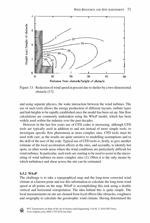
4.2.5 Infl uence of obstacles Sheltering of the anemometer by nearby obstacles such as buildings leads to a dis-tortion of the vertical profi le. The effect of the obstacles depends on their dimen-sions, position and porosity.

Figure 13 sketches out the reduction of wind speed behind an infi nite long two-dimensional obstacle. The hatched area relates to the area around the obstacle which is highly dependent on the actual geometry of the obstacle. The fl ow in this area can only be described by more advanced numerical models such as computa-tional fl uid dynamic (CFD) models.

4.3 Flow models

4.3.1 General Due to the complexity of the vertical extrapolation described above, the predic-tion of the variation of wind speed with height is usually calculated by a computer model, which is specifi cally designed to facilitate accurate predictions of wind farm energy. These models also estimate the energy variation over the site area

Figure 12: Effect of topography on the vertical wind speed profi le gentle hill (top), steep slope (bottom) .



and using separate physics, the wake interaction between the wind turbines. The use of such tools allows the energy production of different layouts, turbine types and hub heights to be rapidly established once the model has been set up. Site fl ow calculations are commonly undertaken using the WAsP model, which has been widely used within the industry over the past decades.

However in the last few years use of CFD codes is increasing, although CFD tools are typically used in addition to and not instead of more simple tools, to investigate specifi c fl ow phenomena at more complex sites. CFD tools must be used with care, as the results are quite sensitive to modelling assumptions and to the skill of the user of the code. Typical use of CFD tools is, fi rstly, to give another estimate of the local acceleration effects at the sites, and secondly, to identify hot spots, in other words areas where the wind conditions are particularly diffi cult for wind turbines. In particular, such tools are starting to be used to assist in the micro-siting of wind turbines on more complex sites [ 1 ]. Often it is the only means by which turbulence and shear across the site can be estimated.

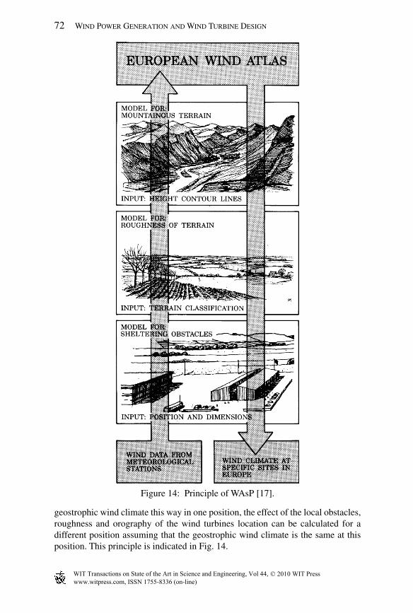
4.3.2 WAsP The challenge is to take a topographical map and the long-term corrected wind climate at a known point and use this information to calculate the long-term wind speed at all points on the map. WAsP is accomplishing this task using a double vertical and horizontal extrapolation. The idea behind this is quite simple. The local measurements on site are cleaned from local effects like obstacles, roughness and orography to calculate the geostrophic wind climate. Having determined the

Figure 13: Reduction of wind speed in percent due to shelter by a two- dimensional obstacle [ 17 ] .



Figure 14: Principle of WAsP [ 17 ] .

geostrophic wind climate this way in one position, the effect of the local obstacles, roughness and orography of the wind turbines location can be calculated for a different position assuming that the geostrophic wind climate is the same at this position. This principle is indicated in Fig. 14.



zD displacement heightProblem areas

5 zD

WasP solution

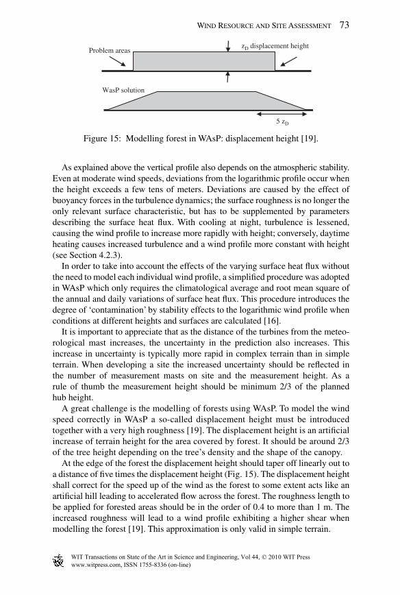
Figure 15: Modelling forest in WAsP: displacement height [ 19 ] .

As explained above the vertical profi le also depends on the atmospheric stability. Even at moderate wind speeds, deviations from the logarithmic profi le occur when the height exceeds a few tens of meters. Deviations are caused by the effect of buoyancy forces in the turbulence dynamics; the surface roughness is no longer the only relevant surface characteristic, but has to be supplemented by parameters describing the surface heat fl ux. With cooling at night, turbulence is lessened, causing the wind profi le to increase more rapidly with height; conversely, daytime heating causes increased turbulence and a wind profi le more constant with height (see Section 4.2.3).

In order to take into account the effects of the varying surface heat fl ux without the need to model each individual wind profi le, a simplifi ed procedure was adopted in WAsP which only requires the climatological average and root mean square of the annual and daily variations of surface heat fl ux. This procedure introduces the degree of ‘contamination’ by stability effects to the logarithmic wind profi le when conditions at different heights and surfaces are calculated [ 16 ].

It is important to appreciate that as the distance of the turbines from the meteo-rological mast increases, the uncertainty in the prediction also increases. This increase in uncertainty is typically more rapid in complex terrain than in simple terrain. When developing a site the increased uncertainty should be refl ected in the number of measurement masts on site and the measurement height. As a rule of thumb the measurement height should be minimum 2/3 of the planned hub height.

A great challenge is the modelling of forests using WAsP. To model the wind speed correctly in WAsP a so-called displacement height must be introduced together with a very high roughness [ 19 ]. The displacement height is an artifi cial increase of terrain height for the area covered by forest. It should be around 2/3 of the tree height depending on the tree’s density and the shape of the canopy.

At the edge of the forest the displacement height should taper off linearly out to a distance of fi ve times the displacement height ( Fig. 15 ). The displacement height shall correct for the speed up of the wind as the forest to some extent acts like an artifi cial hill leading to accelerated fl ow across the forest. The roughness length to be applied for forested areas should be in the order of 0.4 to more than 1 m. The increased roughness will lead to a wind profi le exhibiting a higher shear when modelling the forest [ 19 ]. This approximation is only valid in simple terrain.



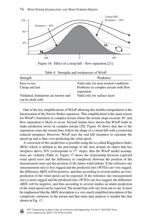
One of the key simplifi cations of WAsP allowing this double extrapolation is the linearisation of the Navier-Stokes equations. This simplifi cation is the main reason for WAsP’s limitation in complex terrain where the terrain slope exceeds 30° and fl ow separation is likely to occur. Several studies have shown that WAsP tends to make prediction errors in complex terrain [ 20 ]. Figure 16 shows that due to the separation zones the stream lines follow the shape of a virtual hill with a somewhat reduced steepness. However, WAsP uses the real hill steepness to calculate the speed-up and is thus over-predicting the wind speed.

A correction of this model bias is possible using the so-called Ruggedness Index (RIX) which is defi ned as the percentage of the area around an object that has steepness above 30% (corresponds to 17° slope), thus the WAsP model assump-tions are violated ( Table 4 ). Figure 17 shows the relationship between expected wind speed error and the difference in complexity between the position of the measurement mast and the position of the future wind turbine. If the reference site (measurement site) is less rugged and the predicted sites (WTGs) are very rugged, the difference Δ RIX will be positive, and thus according to several studies an over-prediction of the wind speed can be expected. If the reference site (measurement site) is more rugged and the predicted sites (WTGs) are less rugged, the difference Δ RIX will be negative, and thus according to several studies an under-prediction of the wind speed can be expected. The model bias will vary from site to site. It must be emphasised that the Δ RIX description is a very much simplifi ed description of the complexity variations in the terrain and that more data analysis is needed like that shown in Fig. 17.

Steepness ~ 40%

Virtual HillSteepness ~ 30%

-100 0 100

120

80

40

Figure 16: Effect of a steep hill – fl ow separation [ 21 ] .

Table 4: Strengths and weaknesses of WAsP.

Strength Weakness

Easy to use Valid only for near-neutral conditionsCheap and fast Problems in complex terrain with fl ow

separationValidated, limitations are known and can be dealt with

Valid only for surface layer



5 Siting and site suitability

5.1 General

During the process of siting (also referred to as micro-siting), the locations of the future wind turbines are determined. Apart from the wind resource this process is driven by a number of other factors such as technical risks, environmental impact, planning restrictions and infrastructure costs.

Technical risks can very often be mitigated by adjusting the layout to suit the site-specifi c conditions. High turbulence as a main driver of fatigue loads can be avoided by maintaining suffi cient distances between the turbines, keeping clear of forests and other turbulence-inducing terrain features like cliffs. Steep terrain slopes should be avoided to reduce stresses on the yaw system and blades and thereby improve the energy output.

5.2 Turbulence

5.2.1 Ambient turbulence The turbulent variations of the wind speed are typically expressed in terms of the standard deviation s u of velocity fl uctuations. This is measured over a 10-min period and normalised by the average wind speed è

— and is called turbulence intensity I u :

uuI

U

s=

(10)

Figure 17: WAsP wind speed prediction error as a function of difference in rug-gedness indices between the predicted and the predictor site [ 20 ].



The variation in this ratio is caused by a large natural variability, but also to some extent because it is sensitive to the averaging time and the frequency response of the sensor used.

Two natural sources of turbulence can be identifi ed: thermal and mechanical. Mechanical turbulence is caused by vertical wind shear and depends on the surface roughness z 0 . The mechanically caused turbulence intensity at a height h in neutral conditions, in fl at terrain and infi nite uniform roughness z 0 can be described as

0

1

ln( / )uI

h z=

(11)

This equation shows an expected decrease of turbulence intensity with increas-ing height above ground level.

Thermal turbulence is caused by convection and depends mainly on the tem-perature difference between ground and air. In unstable conditions, with strong heating of the ground, the turbulence intensity can reach very large values. In sta-ble conditions, with very little vertical exchange of momentum, the turbulence is generally very low. The impact of atmospheric stability is considerable in low to moderate wind speeds.

The turbulence intensity varies with wind speed. It is highest at low wind speeds and shows an asymptotic behaviour towards a constant value at higher wind speeds ( Fig. 18 ). Typical values of I u for neutral conditions in different terrains at typical hub heights of around 80 m are listed in Table 5.

Forests cause a particularly high ambient turbulence and require special atten-tion ( Table 5 ). While special precautions allow estimating the mean wind speed in or near forest with standard fl ow models, the turbulence variations can only be mod-elled with more advanced models. Different concepts are available for more advanced CFD codes. One method to model forest is the simulation via an aerodynamic drag

Figure 18: Turbulence versus wind speed (onshore).



term in the momentum equations, parameterised as a function of the tree height and leaf density. The turbulence model might also be changed to simulate the increased turbulence.

As a rule of thumb measured data indicates that the turbulence intensity created by the forest is signifi cant within a range of fi ve times the forest height vertically and 500 m downstream from the forest edge in a horizontal direction. Outside these boundaries the ambient turbulence intensity is rapidly approaching normal values [ 22 ].

In or near forest, the mechanically generated turbulence intensity increases in high wind speeds due to the increasing movement of the canopy. A similar phe-nomenon can be observed in offshore conditions where increasing waves lead to increased turbulence in high wind speeds ( Fig. 19 ). The increasing turbulence with increasing wind speed is of great importance when calculating the extreme gusts for a site.

Table 5: Typical hub height turbulence intensities for different land covers.

Land cover Typical I u (%)

Offshore 8Open grassland 10Farming land with wind breaks 13Forests 20 or more

Tur

bule

nce

inte

nsity

Windspeed (m/s)

0 5 10 15 20 25 30

0.08

0.1

0.12

0.14

0.06

8 m48 m

Figure 19: Turbulence versus wind speed (offshore) [ 23 ].



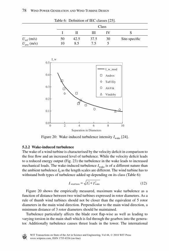
5.2.2 Wake-induced turbulence The wake of a wind turbine is characterised by the velocity defi cit in comparison to the free fl ow and an increased level of turbulence. While the velocity defi cit leads to a reduced energy output ( Fig. 23 ) the turbulence in the wake leads to increased mechanical loads. The wake-induced turbulence I wake is of a different nature than the ambient turbulence I 0 as the length scales are different. The wind turbine has to withstand both types of turbulence added up depending on its class ( Table 6 ):

2 2

wind farm 0 wakeI I I= + (12)

Figure 20 shows the empirically measured, maximum wake turbulence as a function of distance between two wind turbines expressed in rotor diameters. As a rule of thumb wind turbines should not be closer than the equivalent of 5 rotor diameters in the main wind direction. Perpendicular to the main wind direction, a minimum distance of 3 rotor diameters should be maintained.

Turbulence particularly affects the blade root fl ap-wise as well as leading to varying torsion in the main shaft which is fed through the gearbox into the genera-tor. Additionally turbulence causes thrust loads in the tower. The international

Table 6: Defi nition of IEC classes [ 25 ].

Class

I II III IV S

U ref (m/s) 50 42.5 37.5 30 Site-specifi c U ave (m/s) 10 8.5 7.5 5

0.0

0.1

0.2

0.3

0.4

0.5

0 2 4 6 8 10

Separation in Diameters

I_w

I_w_mod

Andros

Taff Ely

AlsVik

Vindeby

Figure 20: Wake-induced turbulence intensity I wake [ 24 ] .



design standard IEC [ 25 ] assumes a maximum level of total turbulence of 18% for a wind turbine designed for high turbulence.

5.3 Flow inclination

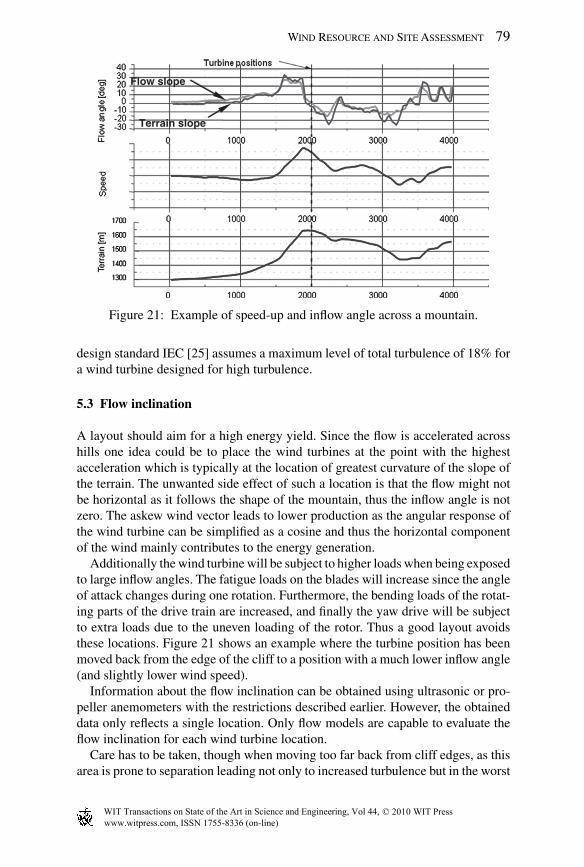
A layout should aim for a high energy yield. Since the fl ow is accelerated across hills one idea could be to place the wind turbines at the point with the highest acceleration which is typically at the location of greatest curvature of the slope of the terrain. The unwanted side effect of such a location is that the fl ow might not be horizontal as it follows the shape of the mountain, thus the infl ow angle is not zero. The askew wind vector leads to lower production as the angular response of the wind turbine can be simplifi ed as a cosine and thus the horizontal component of the wind mainly contributes to the energy generation.

Additionally the wind turbine will be subject to higher loads when being exposed to large infl ow angles. The fatigue loads on the blades will increase since the angle of attack changes during one rotation. Furthermore, the bending loads of the rotat-ing parts of the drive train are increased, and fi nally the yaw drive will be subject to extra loads due to the uneven loading of the rotor. Thus a good layout avoids these locations. Figure 21 shows an example where the turbine position has been moved back from the edge of the cliff to a position with a much lower infl ow angle (and slightly lower wind speed).

Information about the fl ow inclination can be obtained using ultrasonic or pro-peller anemometers with the restrictions described earlier. However, the obtained data only refl ects a single location. Only fl ow models are capable to evaluate the fl ow inclination for each wind turbine location.

Care has to be taken, though when moving too far back from cliff edges, as this area is prone to separation leading not only to increased turbulence but in the worst

Terrain slope

Flow slope

Figure 21: Example of speed-up and infl ow angle across a mountain .



case to reverse fl ow imposing the potential of serious damage to the wind turbine ( Fig. 22 ). The vertical and horizontal extent of such unsuitable areas can be estimated using CFD.

The international design standard IEC [ 25 ] assumes an infl ow angle of maximum 8° for load calculations.

5.4 Vertical wind speed gradient

The loads on the rotor depend on the wind speed difference between the bottom and the top of the rotor. The gradient is normally expressed by the wind shear exponent a from the power law (eqn ( 6 )). Most load cases assume a gradient of 0.2 between the bottom and the top of the rotor [ 25 ]. Note that in some cases, loads will be larger for very small or negative a .

The gradient causes changing loads of the blades as the angle of attack changes with each rotation. Thus the gradient adds to the fatigue loads of the blade roots. Furthermore the rotating parts of the drive train are stressed. The gradient is affected by four different phenomena:

• Terrain slope . The logarithmic profi le can be heavily distorted by terrain slopes. While in fl at terrain the wind speed increases with height, steep slopes might lead to a decrease with height. This is particularly likely for sites where the fl ow separates and does not follow the shape of the terrain anymore ( Fig. 12 ). As a consequence the wind speed exponent might exceed the design limit in some sections of the rotor. • Roughness/obstacles . If wind turbines are located closely behind obstacles like for example a forest the vertical wind speed profi le might be again heavily dis-torted and areas of the rotor are exposed to large gradients. The degree of defor-mation of the profi le depends not only on the geometry of the obstacle but also on its porosity. • Layout . As explained above, the wake of a wind turbine is a conical area behind the rotor with increased turbulence and reduced wind speed since the rotor of the wind turbine has extracted kinetic energy from the fl ow. Figure 23 shows the effect of the wake on the profi le, where the dotted line represents the free fl ow and the straight line the profi le 5.3 rotor diameter behind the wind turbine.

Figure 22: An example of fl ow separation over a cliff .



It can clearly be seen that some areas of the deformed profi le show very large gradients. If the wind turbines operate in part wake situations ( Fig. 24 ), the wind turbines behind the front row will not only be exposed to vertical gradients but also to horizontal gradients which add signifi cantly to the loads. • Atmospheric stability . As explained above, the vertical wind speed profi le de-pends on the vertical temperature profi le. With increasing heating of the ground (unstable conditions) the turbulence increases and therefore the profi le is being “smoothed” out. This leads to a steep wind speed profi le characterised by very little increase of wind speed with height. Stable conditions in contrast are characterised by a very fl at profi le with signifi cant wind speed gradients (see Fig. 11 ). Depending on the prevailing atmospheric stability of the site the gradient of 0.2 assumed for most load cases can be exceeded. Additionally in stable conditions signifi cant wind direction shears are common.

Figure 24: Horizontal gradient due to part wake operation .

Figure 23: Vertical wind profi le in front and behind a wind turbine [ 16 ] .



An optimised layout can avoid excessive gradients related to the fi rst three phe-nomena by staying clear from steep slopes, obstacles and allow a suffi cient spacing between the wind turbines.

The gradient is often determined by measurements. Care has to be taken when the measurement height is lower than hub height since the wind shear exponent is a function of height, thus a gradient measured at lower height is not representative for higher heights. Be also aware of the fact that because the measured wind speed differences can be relatively small, the resulting measurement uncertainties can become quite signifi cant. The preferred method in these cases is to model the wind speed profi le using fl ow models.

6 Site classifi cation

6.1 Introduction

When designing wind turbines a set of assumptions describing the wind climate on-site is made. As the robustness of a wind turbine is directly related to the costs of the machine, a system has become common of grouping sites into four different categories to allow cost optimisation of the wind turbines. The site class depends on the mean wind speed and extreme wind speed at hub height referred to as IEC classes [ 25 ]. Furthermore three different turbulence classes have been introduced, for low, medium and high turbulence sites. The term extreme wind or U ref is used for the maximum 10-min average wind speed with a recurrence of 50 years at hub height. Please note that U ref is not related to the mean wind speed.

6.2 Extreme winds

Selecting a suitable turbine for a site requires knowledge about the expected extreme wind in the form of the maximum 10-min average wind speed at hub height with a recurrence period of 50 years ( U ref according to the IEC 61400-1 [ 25 ]). While local building codes frequently generalise the amplitude of extreme events across large areas, on-site measured wind data allows for a more precise site-specifi c predic-tion of the expected 50-year event. A number of methods offer the possibility to estimate the on-site 50-year maximum 10-min wind speed from available shorter term on-site data. The IEC 61400-1 does not prescribe any preferred method for this purpose though.

Under certain assumptions, a Gumbel analysis [ 26 ] can be applied to predict the 50-year extreme wind speed on the basis of the measured on-site maximum wind speeds. If these assumptions are correct, then the measured maximum wind speeds should resemble a straight line in the Gumbel plot.

Different methodologies are available to extract extreme events from a short-term data set and further to fi t the Gumbel distribution to these extremes. The parameters describing the Gumbel distribution are generally determined from the linear fi t in a Gumbel plot. Hereby the so-called reduced variant



(transformed probability of non-exceedence) is plotted versus wind speed. The reduced variant (probability) can be expressed in different ways leading to different plotting positions. Furthermore, a variety of fi tting options are avail-able leading to a vast number of different results [ 27 ]. However, all methods have one problem in common. The resulting 50-year estimate is highly corre-lated to the highest measured wind speed event of the time series used for the analysis [ 28 ].

The European Wind Turbine Standard, EWTS [ 29 ] offers an option to estimate the extreme wind based on the wind speed distribution on site rather than a mea-sured time series. It suggests a link between the shape of the wind distribution and the extreme wind. The EWTS relates a ratio determined by the Weibull k factor to the annual average wind speed to estimate the 50-year extreme wind speed. This factor is 5 for k = 1.75, <5 for higher values of k and >5 for lower k values (i.e. high values for distributions with long tails, and low values for distributions with lower frequency of high wind speeds). The extreme wind is calculated as this factor times the yearly averaged wind speed.

The extreme 3-s gust or also called design wind speed of the wind turbine ( U e50 ) is a function of the U ref and the turbulence intensity. The extreme gust is estimated using the relationship, where the turbulence intensity I ext is a high wind speed turbulence value estimated from the measured data:

exte50 ref(1 2.8 )U U I= + (13)

This relationship is based on experimental data as well as theoretical work ( Fig. 25 ). As mentioned in Section 5.2.1 care has to be taken in offshore and forest situa-tions as the turbulence intensity does not show asymptotic behaviour but increases with increasing wind speed. It is thus much more diffi cult to estimate I ext under these conditions.

Figure 25: Measured gust as a function of wind speed [ 16 ] .



7 Energy yield and losses

7.1 Single wind turbine

The power production varies with the wind speed that strikes the rotor. The wind speed at hub height is normally used as a reference for the power response of the wind turbine. Knowing the power curve of a wind turbine P ( u ), the mean power pro-duction can be estimated using the probability density function of the wind speed at hub height f ( u ), which is typically expressed as a Weibull distribution (see eqn ( 3 )):

1

0 0

( ) ( )d exp ( )dk k

k u uP f u P u u P u u

A A A

−∞ ∞ ⎛ ⎞⎛ ⎞ ⎛ ⎞= = −⎜ ⎟⎜ ⎟ ⎜ ⎟⎝ ⎠ ⎝ ⎠⎝ ⎠∫ ∫

(14)

This integral cannot be computed analytically and thus has to be solved numer-ically. For this purpose the power curve is divided into a suffi cient number of lin-ear sections, typically for 0.5 m/s steps. The power output can now be calculated by summing up the produced energy for each wind speed bin.

Care has to be taken as the power of the wind is proportional to the air density. A power curve normally refers to an air density of 1.225 kg/m 3 which corresponds to a temperature of 15°C at sea level. A higher elevation and/or a warmer site will lead to a lower air density and thus to a lower energy output.

Special considerations should be given to the fact that a number of site-specifi c parameters infl uence the power curve and thus the energy yield most signifi cantly turbulence and wind shear [ 30 ].

Another way of stating the annual energy output from a wind turbine is to look at the capacity factor for the turbine in its particular location. By capacity factor we mean its actual annual energy output divided by the theoretical maximum out-put if the machine were running at its rated (maximum) power during all of the 8760 h of the year. The capacity factors may theoretically vary from 0 to 100%, but in practice they will mostly be around 30–40%.

7.2 Wake and other losses

As mentioned in Section 5.2.2 and shown in Fig. 23 the wake of a wind turbine is characterised by a velocity defi cit. This will lead to a reduced effi ciency of any wind turbine operating in its wake. The so-called park loss is dependent on the thrust curve of the rotor, on the wake decay constant (which in turn is a function of the ambient turbulence intensity), and the distance between the turbines. High ambient turbulence intensity will lead to an increased mixing between the wake and the surrounding undisturbed fl ow. As a consequence the opening angle of the wake increases, thus resulting in smaller park losses than low turbulence situations.

Two models are commonly used in the industry, the N.O. Jensen model and the Eddy-Viscosity model of Ainslie [ 32 ]. The N.O. Jensen model is a simple, single wake kinematic model, in terms of an initial velocity defi cit and a wake decay constant. It is based on the assumption that the wake right behind the wind turbine



has a starting diameter equal to the rotor diameter and is linearly expanding as a function of the downwind distance. The Ainslie model is based on a numerical solution of the Navier-Stokes equations with an eddy viscosity closure in cylindri-cal coordinates. The eddy viscosity is described by the turbulent mixing due to the induced turbulence, generated within the shear layer of the wake, and the ambient turbulence [ 33 ].

Other sources of losses could be related to availability, electrical losses, high wind hysteresis, environmental conditions like icing and blade degradation and curtailments, of which wind sector management is the most common one. As explained earlier turbine loading is infl uenced by the wake effects from nearby machines. For some wind farms with particularly close spacing, it may be neces-sary to shut down certain wind turbines for certain wind directions. Typically this is done in a wind climate with a very dominant and narrow main wind direction.

7.3 Uncertainty

Uncertainty analysis is an important part of any assessment of the long-term energy production of a wind farm. The most important contributors to the uncertainty are:

on-site wind speed measurements • long-term correction • fl ow modelling • performance of the wind turbine • park losses •

Behind each point a vast number of aspects have to be considered and quantifi ed including anemometer calibration, mounting effects, inter-annual variability, qual-ity of the long-term data, vertical and horizontal extrapolation, quality of the topo-graphic input, power curve uncertainty, wake model, etc. Some inspiration can be found in [ 34 ].

R eferences

[1] European Wind Energy Association. Wind Energy – The Facts. ISBN-978-1-84407-710-6, 2009.

[2] IEC 61400-12-1. Wind Turbines Part 12-1: Power performance measure-ments of electricity producing wind turbines , 2005.

[3] IEA. Recommended practices for wind turbine testing, Part 11: Wind speed measurement and use of cup anemometry , 1999.

[4] Lindelöw, P., Courtney, M., Mortensen, N.G. & Wagner, R., Are Lidars good enough? Accuracy of AEP predictions in fl at terrain generated from measure-ments by conically scanning wind sensing Lidars. Proc. of European Wind Energy Conf. , Marseille, France, 2009.

[5] Brock, F.V. & Richardson, S.J., Meteorological Measurement Systems, Oxford University Press, 2001.



[6] Monna, W.A.A., Comparative investigation of dynamic properties of some propeller vanes. WR 78-11, KNMI, The Netherlands, 1978.

[7] Bradley, S., Antoniou, I., von Hünerbein, S., Kindler, D., de Noord, M. & Jørgensen, H., Sodar calibration procedure, Final reporting WP3, EU WISE project NNE5-2001-297, University of Salford, 2005.

[8] Antoniou, I., Jørgensen, H.E., Ormel, F., Bradley, S., von Hünerbein, S., Emeis, S. & Warmbier, G., On the theory of Sodar measurement techniques. Risø-R-1410, Risø National Laboratory, Roskilde, Denmark, 2003.

[9] Antoniou, I., Jørgensen, H.E., Bradley, S.G., von Hunerbein, S., Cutler, N., Kindler, D., de Noord, M. & Warmbier, G., The profi ler inter-comparison experiment (PIE). Proc. of European Wind Energy Conf. , London, UK, 2004.

[10] Courtney, M., Wagner, R. & Lindelöw, P., Commercial Lidar profi lers for wind energy. A comparative guide . Proc. of European Wind Energy Conf. , Brussels, Belgium, 2008.

[11] Antoniou, I., Jørgensen, H.E., Mikkelsen, T., Pedersen, T.F., Warmbier, G. & Smith, D., Comparison of wind speed and power curve measurements using cup anemometer, a Lidar and a Sodar. Proc. of European Wind Energy Conf. , London, UK, 2004.

[12] Foussekis, D. & Georgakopoulos, T., Investigating wind fl ow properties in complex terrain using 3 Lidars and a meteorological mast. Proc. of European Wind Energy Conf. , Marseille, France, 2009.

[13] Bingöl, F., Mann, J. & Foussekis, D., Lidar performance in complex terrain modelled by WAsP Engineering . European Wind Energy Conf. , Marseille, France, 2009.

[14] Dupont, E., Lefranc, Y. & Sécolier, C., A Sodar campaign in complex terrain for data quality evaluation and methodological investigations. Proc. of Euro-pean Wind Energy Conf. , Marseille, France, 2009.

[15] Petersen, E.L., Troen, I., Frandsen, S. & Hedegaard, K., Wind atlas for Denmark – A rational method for wind energy siting. Risø-R-428, Risø National Laboratory, Roskilde, Denmark, 1981.

[16] Petersen, E.L., Mortensen, N.G., Landberg, L., Højstrup, J. & Frank, H.P., Wind power meteorology. Risø-R-1206, Risø National Laboratory, Roskilde, Denmark, 1997.

[17] Troen, I. & Petersen, E.L., European wind atlas, ISBN 87-550-1482-8, Risø National Laboratory, Roskilde, Denmark, 1989.

[18] Lange, B., Modelling the marine boundary layer for offshore wind power utilization, Ph.D. thesis, University Oldenburg, Germany, 2002.

[19] Dellwik, E., Jensen, N.O. & Landberg, L., Wind and forests – general rec-ommendations for using WasP, 2004, http://www.bwea.com/pdf/trees/Risoe.pdf

[20] Mortensen, N.G., Bowen, A.J. & Antoniou, I., Improving WAsP predictions in (too) complex terrain. Proc. of European Wind Energy Conf. , Athens, Greece, 2006.

[21] Wood, N., The onset of fl ow separation in neutral, turbulent fl ow over hills. Boundary Layer Meteorology , 76 , pp. 137–164, 1995.



[22] Pedersen, H.S. & Langreder, W., Forest-added turbulence: a parametric study on turbulence. Journal of Physics , Conference Series 75 – 012062, 2007.

[23] Barthelmie, R., Hansen, O.F., Enevoldsen, K., Motta, M., Pryor, S., Højstrup, J., Frandsen, S., Larsen, S. & Sanderhoff, P., Ten years of measurements of offshore wind farms – what have we learnt and where are uncertainties? The Science of Making Torque from Wind, Delft, 2004.

[24] Frandsen, S. & Thøgersen, M., Integrated fatigue loading for wind turbines in wind farms by combining ambient turbulence and wakes. Wind Engineering , 23( 6 ) , pp. 327–339, 1999.

[25] IEC 61400-1. Wind Turbines Part 1: Design requirements , 2005. [26] Gumbel, E.J., Statistics of Extremes , Columbia University Press, 1958. [27] Palutikof, J.P., Brabson, B.B., Lister, D.H. & Adcock, S.T., A review of

methods to calculate extreme wind speeds. Meteorological Applications , 6 , pp. 119–132, 1999.

[28] Langreder, W., Højstrup, J. & Svenningsen, L., Extreme wind estimates with modest uncertainty – a contradiction? Proc. of Windpower Conf. , Chicago, 2009.

[29] Dekker, J.W.M. & Pierik, J.T.G., European Wind Turbine Standard II . ECN-C-99-073, The Netherlands, 1999.

[30] Langreder, W., Kaiser, K., Hohlen, H. & Højstrup, J., Turbulence correc-tions for power curves . Proc. of European Wind Energy Conf. , London, UK, 2004.

[31] Antoniou, I. & Pedersen, S.M., Infl uence of turbulence, wind shear and low level jets on the power curve and the AEP of a wind turbine. Proc. of Euro-pean Wind Energy Conf. , Marseille, France, 2009.

[32] Ainslie, J.F., Calculating the fl owfi eld in the wake of wind turbines. Journal of Wind Engineering and Industrial Aerodynamics , 27 , pp. 213–224, 1988.

[33] Zigras, D. & Mönnich, K., Farm effi ciencies in large wind farms. Proc. of Windpower Conf. , Los Angeles, USA, 2007.

[34] Albers, A., Uncertainty analysis and optimisation of energy yield predictions as basis for risk evaluation of wind farm projects. Proc. of European Wind Energy Conf. , Madrid, Spain, 2003.


chapter 2 wind resource and site assessment...chapter 2 wind resource and site assessment wiebke...

Documents