chapter 3 a new directional over current...
TRANSCRIPT
41
CHAPTER 3
A NEW DIRECTIONAL OVER CURRENT RELAYING SCHEME FOR DISTRIBUTION FEEDERS IN THE PRESENCE OF DG
3.1 INTRODUCTION
In plain radial feeders, the non-directional relays are used as they operate when the CT
secondary current exceeds the threshold value of pickup setting in relays. This type of relay
operates irrespective of the direction of current flow.
The feeders other than plain radial feeders are not protected by the non-directional
overcurrent relays as they require the creation of zones. The protection of such parallel feeders
or double-end-fed feeders is protected by the directional relays. By introducing the directional
feature in relays, uninterrupted supply can be made possible at all load points connected in
parallel/ring system.
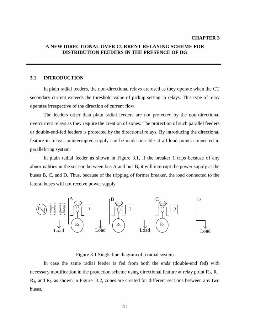
In plain radial feeder as shown in Figure 3.1, if the breaker 1 trips because of any
abnormalities in the section between bus A and bus B, it will interrupt the power supply at the
buses B, C, and D. Thus, because of the tripping of former breaker, the load connected to the
lateral buses will not receive power supply.
Figure 3.1 Single line diagram of a radial system
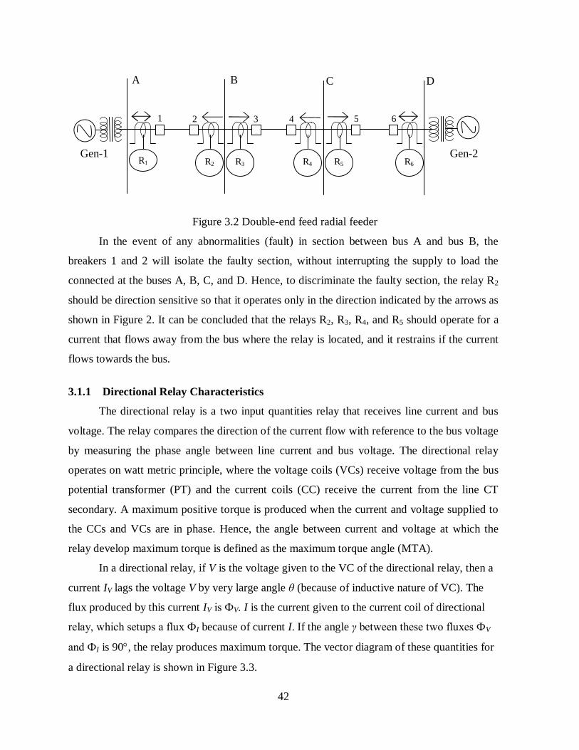
In case the same radial feeder is fed from both the ends (double-end fed) with
necessary modification in the protection scheme using directional feature at relay point R2, R3,
R4, and R5, as shown in Figure 3.2, zones are created for different sections between any two
buses.
Load Load
B C D A
R1 R3 R5
1 2 3
Load Load
42
Figure 3.2 Double-end feed radial feeder
In the event of any abnormalities (fault) in section between bus A and bus B, the
breakers 1 and 2 will isolate the faulty section, without interrupting the supply to load the
connected at the buses A, B, C, and D. Hence, to discriminate the faulty section, the relay R2
should be direction sensitive so that it operates only in the direction indicated by the arrows as
shown in Figure 2. It can be concluded that the relays R2, R3, R4, and R5 should operate for a
current that flows away from the bus where the relay is located, and it restrains if the current
flows towards the bus.
3.1.1 Directional Relay Characteristics
The directional relay is a two input quantities relay that receives line current and bus
voltage. The relay compares the direction of the current flow with reference to the bus voltage
by measuring the phase angle between line current and bus voltage. The directional relay
operates on watt metric principle, where the voltage coils (VCs) receive voltage from the bus
potential transformer (PT) and the current coils (CC) receive the current from the line CT
secondary. A maximum positive torque is produced when the current and voltage supplied to
the CCs and VCs are in phase. Hence, the angle between current and voltage at which the
relay develop maximum torque is defined as the maximum torque angle (MTA).
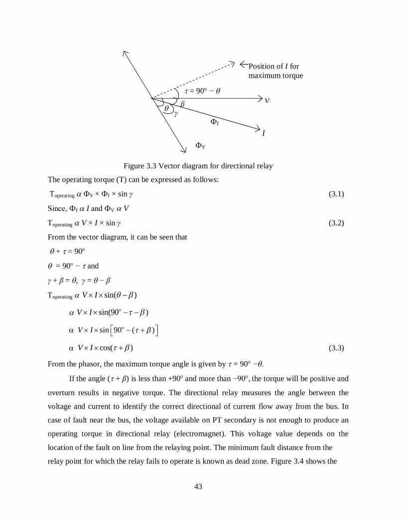
In a directional relay, if V is the voltage given to the VC of the directional relay, then a
current IV lags the voltage V by very large angle θ (because of inductive nature of VC). The
flux produced by this current IV is ФV. I is the current given to the current coil of directional
relay, which setups a flux ФI because of current I. If the angle γ between these two fluxes ФV
and ФI is 90, the relay produces maximum torque. The vector diagram of these quantities for
a directional relay is shown in Figure 3.3.
6 5 4 3 2 1
C B A
R2 R1 R3
D
R4
1 1
R5 R6
1 Gen-1 Gen-2
43
Figure 3.3 Vector diagram for directional relay
The operating torque (T) can be expressed as follows:
operating ФV × ФI × sin γ (3.1)
Since, ФI I and ФV V
operating V × I × sin γ (3.2)
From the vector diagram, it can be seen that
+ = 90
= 90 − and
γ + β = , γ = − β
operating sin( )V I
sin(90 )V I
sin 90 ( )V I
cos( )V I (3.3)
From the phasor, the maximum torque angle is given by = 90 −.
If the angle ( + β) is less than +90 and more than −90, the torque will be positive and
overturn results in negative torque. The directional relay measures the angle between the
voltage and current to identify the correct directional of current flow away from the bus. In
case of fault near the bus, the voltage available on PT secondary is not enough to produce an
operating torque in directional relay (electromagnet). This voltage value depends on the
location of the fault on line from the relaying point. The minimum fault distance from the
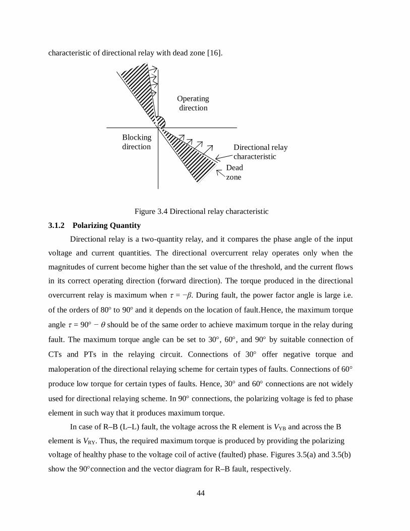
relay point for which the relay fails to operate is known as dead zone. Figure 3.4 shows the
Position of I for maximum torque
I
V γ
ФI
β = 90 −
0
ФV
44
characteristic of directional relay with dead zone [16].
Figure 3.4 Directional relay characteristic
3.1.2 Polarizing Quantity
Directional relay is a two-quantity relay, and it compares the phase angle of the input
voltage and current quantities. The directional overcurrent relay operates only when the
magnitudes of current become higher than the set value of the threshold, and the current flows
in its correct operating direction (forward direction). The torque produced in the directional
overcurrent relay is maximum when = −β. During fault, the power factor angle is large i.e.
of the orders of 80 to 90 and it depends on the location of fault.Hence, the maximum torque
angle = 90 − should be of the same order to achieve maximum torque in the relay during
fault. The maximum torque angle can be set to 30, 60, and 90 by suitable connection of
CTs and PTs in the relaying circuit. Connections of 30 offer negative torque and
maloperation of the directional relaying scheme for certain types of faults. Connections of 60
produce low torque for certain types of faults. Hence, 30 and 60 connections are not widely
used for directional relaying scheme. In 90 connections, the polarizing voltage is fed to phase
element in such way that it produces maximum torque.
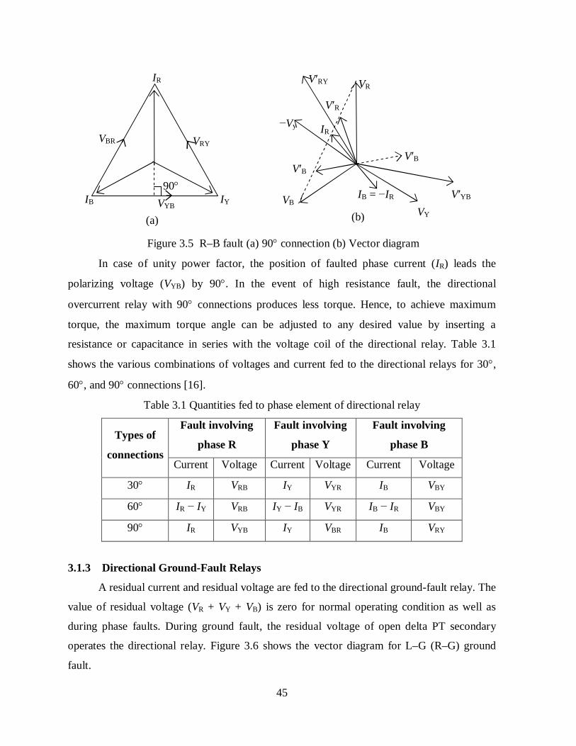
In case of R–B (L–L) fault, the voltage across the R element is VYB and across the B
element is VRY. Thus, the required maximum torque is produced by providing the polarizing
voltage of healthy phase to the voltage coil of active (faulted) phase. Figures 3.5(a) and 3.5(b)
show the 90connection and the vector diagram for R–B fault, respectively.
Blocking direction
Dead zone
Operating direction
Directional relay characteristic
45
Figure 3.5 R–B fault (a) 90 connection (b) Vector diagram
In case of unity power factor, the position of faulted phase current (IR) leads the
polarizing voltage (VYB) by 90. In the event of high resistance fault, the directional
overcurrent relay with 90 connections produces less torque. Hence, to achieve maximum
torque, the maximum torque angle can be adjusted to any desired value by inserting a
resistance or capacitance in series with the voltage coil of the directional relay. Table 3.1
shows the various combinations of voltages and current fed to the directional relays for 30,
60, and 90 connections [16].
Table 3.1 Quantities fed to phase element of directional relay
Types of
connections
Fault involving
phase R
Fault involving
phase Y
Fault involving
phase B
Current Voltage Current Voltage Current Voltage
30 IR VRB IY VYR IB VBY
60 IR − IY VRB IY − IB VYR IB − IR VBY
90 IR VYB IY VBR IB VRY
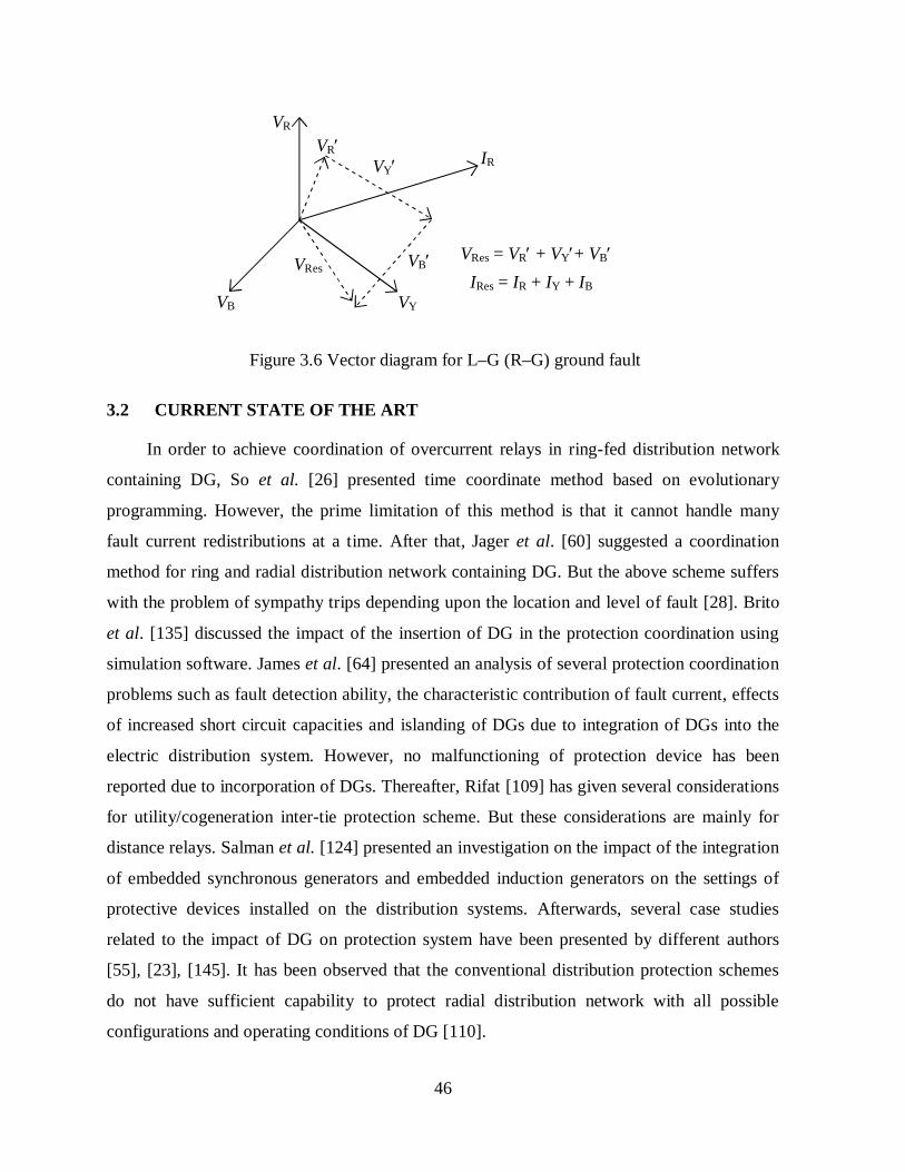
3.1.3 Directional Ground-Fault Relays
A residual current and residual voltage are fed to the directional ground-fault relay. The
value of residual voltage (VR + VY + VB) is zero for normal operating condition as well as
during phase faults. During ground fault, the residual voltage of open delta PT secondary
operates the directional relay. Figure 3.6 shows the vector diagram for L–G (R–G) ground
fault.
(a)
V′B
V′RY
−Vy IR
V′R
VR
VB
V′B
IB = −IR VY
V′YB VYB
VRY VBR
IR
IY IB 90
(b)
46
Figure 3.6 Vector diagram for L–G (R–G) ground fault
3.2 CURRENT STATE OF THE ART
In order to achieve coordination of overcurrent relays in ring-fed distribution network
containing DG, So et al. [26] presented time coordinate method based on evolutionary
programming. However, the prime limitation of this method is that it cannot handle many
fault current redistributions at a time. After that, Jager et al. [60] suggested a coordination
method for ring and radial distribution network containing DG. But the above scheme suffers
with the problem of sympathy trips depending upon the location and level of fault [28]. Brito
et al. [135] discussed the impact of the insertion of DG in the protection coordination using
simulation software. James et al. [64] presented an analysis of several protection coordination
problems such as fault detection ability, the characteristic contribution of fault current, effects
of increased short circuit capacities and islanding of DGs due to integration of DGs into the
electric distribution system. However, no malfunctioning of protection device has been
reported due to incorporation of DGs. Thereafter, Rifat [109] has given several considerations
for utility/cogeneration inter-tie protection scheme. But these considerations are mainly for
distance relays. Salman et al. [124] presented an investigation on the impact of the integration
of embedded synchronous generators and embedded induction generators on the settings of
protective devices installed on the distribution systems. Afterwards, several case studies
related to the impact of DG on protection system have been presented by different authors
[55], [23], [145]. It has been observed that the conventional distribution protection schemes
do not have sufficient capability to protect radial distribution network with all possible
configurations and operating conditions of DG [110].
VRes
IR
VR VR
VY
VY
VB
VB
VRes = VR + VY+ VB IRes = IR + IY + IB
47
Tong and his co-worker [45] presented a concept of FCL (Fault Current Limiter) to
limit the effect of DG on the coordinated relay protection scheme in a radial system. But the
proposed concept can be applicable only up to certain tolerable levels with reference to
tripping time. Manjula et al. [79] proposed an inverse time admittance relay based on line
admittance measurement to protect a distribution network with converter interfaced DG.
However, relay operation may be restrained beyond predefined value of fault resistance.
Further, the cost of distance relays is comparatively higher than overcurrent relays. However,
none of these schemes completely solved the problem of miscoordination between relay in
radial distribution systems in the presence of DG.
In order to avoid most of the above drawbacks, an attempt has been made to
demonstrate the concept of directional relay for the protection of radial distribution network
containing DGs. The proposed work was supported with the developed prototype of 3-phase
radial distribution system in laboratory environment along with their comparative evaluation
with the results obtained using PSCAD/EMTDC software package.
3.3 THE PROPOSED DIRECTIONAL RELAYING SCHEME
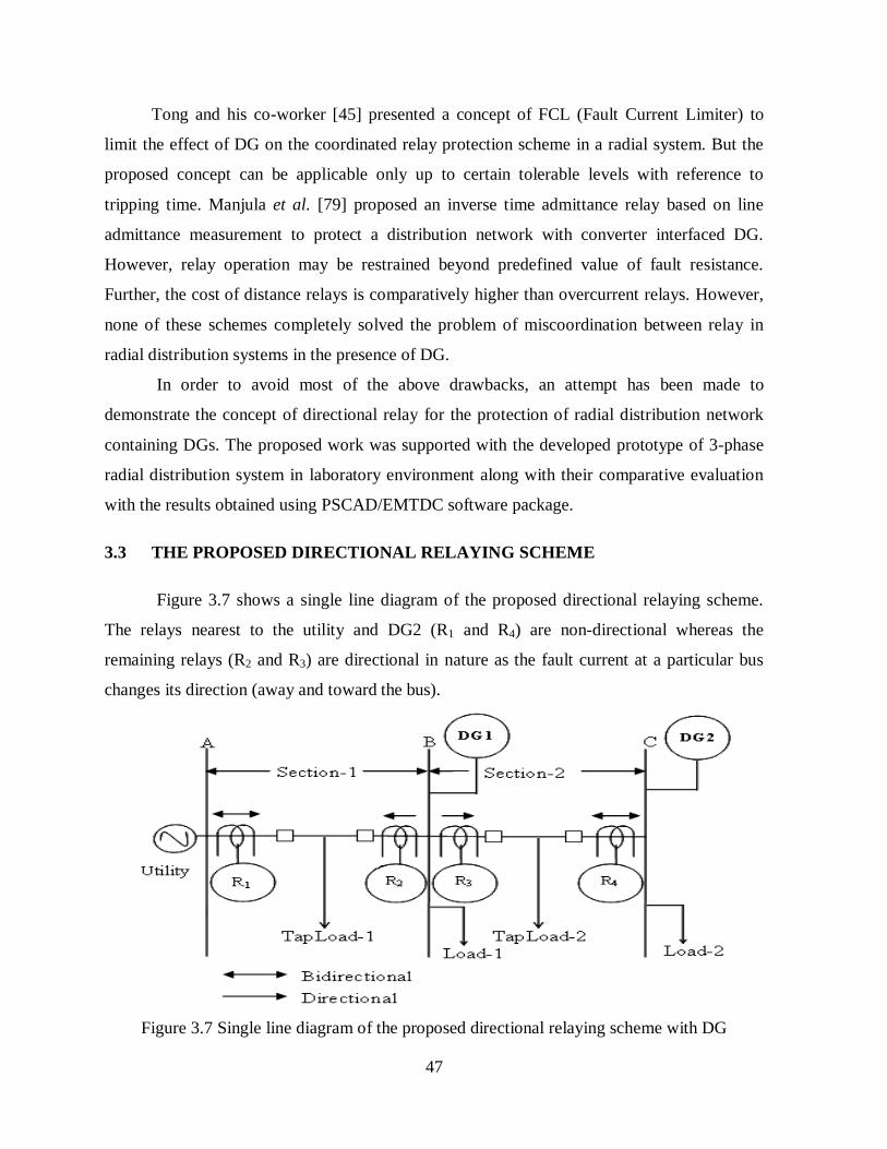
Figure 3.7 shows a single line diagram of the proposed directional relaying scheme.
The relays nearest to the utility and DG2 (R1 and R4) are non-directional whereas the
remaining relays (R2 and R3) are directional in nature as the fault current at a particular bus
changes its direction (away and toward the bus).
Figure 3.7 Single line diagram of the proposed directional relaying scheme with DG
48
The directional feature is gained by comparing the direction of current flow in the line with
reference to the bus voltage. Thus, the directional overcurrent relay operates only when the
current flowing through the relay is in its correct direction and more than its pickup setting.
With reference to Figure 3.7, for a fault in section-1, relays R1 and R2 operate and disconnect
the section-1 only, while the section-2 remains in healthy condition.
During the implementation of the proposed scheme in the laboratory environment and
also in the computer simulation, the following assumptions have been carried out.
1. In the development of laboratory prototype, authors have used class one CTs and PTs
whereas for computer simulation in PSCAD/EMTDC, available “Jiles-Atherton” CT
model has been used.
2. The effect of saturation of CT on the performance of the proposed scheme during
computer simulation in PSCAD/EMTDC software package has not been considered.
On the other hand, the effect of CT saturation, depending upon the magnitude of fault
current, will affect the performance of relays used in developed laboratory prototype.
3. Relays used in the developed laboratory prototype are electromechanical in nature
whereas in the computer simulation, modules of static relays having similar
characteristic to that of electromechanical relays used in developed laboratory
prototype are used.
4. In the proposed developed laboratory prototype, state electricity board supply has been
used as utility. On the other hand, three-phase synchronous generators having different
capacities have been used as DGs.
As some system structure is required to produce realistic data, a small portion of large
power distribution system has been used. Due to practical limitations, only two sections for
the implementation of the proposed scheme in the laboratory have been chosen. However, the
idea of the proposed directional protection scheme can be further extended to larger
distribution network.
3.4 DEVELOPED LABORATORY PROTOTYPE OF THE PROPOSED
DIRECTION RELAYING SCHEME
Figure 3.8 shows laboratory prototype of the proposed directional relaying scheme.
Synchronous generator has been used as DG which is connected at Bus-B and Bus-C whereas
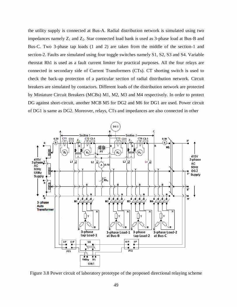
49
the utility supply is connected at Bus-A. Radial distribution network is simulated using two
impedances namely Z1 and Z2. Star connected load bank is used as 3-phase load at Bus-B and
Bus-C. Two 3-phase tap loads (1 and 2) are taken from the middle of the section-1 and
section-2. Faults are simulated using four toggle switches namely S1, S2, S3 and S4. Variable
rheostat Rh1 is used as a fault current limiter for practical purposes. All the four relays are
connected in secondary side of Current Transformers (CTs). CT shorting switch is used to
check the back-up protection of a particular section of radial distribution network. Circuit
breakers are simulated by contactors. Different loads of the distribution network are protected
by Miniature Circuit Breakers (MCBs) M1, M2, M3 and M4 respectively. In order to protect
DG against short-circuit, another MCB M5 for DG2 and M6 for DG1 are used. Power circuit
of DG1 is same as DG2. Moreover, relays, CTs and impedances are also connected in other
Figure 3.8 Power circuit of laboratory prototype of the proposed directional relaying scheme
50
two phases. However, due to complexity, it has not shown in Figure 3.8. Detailed
specifications of the different components used in the said laboratory prototype are given in
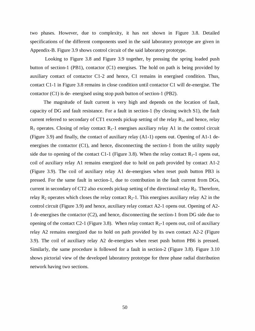
Appendix-B. Figure 3.9 shows control circuit of the said laboratory prototype.
Looking to Figure 3.8 and Figure 3.9 together, by pressing the spring loaded push
button of section-1 (PB1), contactor (C1) energises. The hold on path is being provided by
auxiliary contact of contactor C1-2 and hence, C1 remains in energised condition. Thus,
contact C1-1 in Figure 3.8 remains in close condition until contactor C1 will de-energise. The
contactor (C1) is de- energised using stop push button of section-1 (PB2).
The magnitude of fault current is very high and depends on the location of fault,
capacity of DG and fault resistance. For a fault in section-1 (by closing switch S1), the fault
current referred to secondary of CT1 exceeds pickup setting of the relay R1, and hence, relay
R1 operates. Closing of relay contact R1-1 energises auxiliary relay A1 in the control circuit
(Figure 3.9) and finally, the contact of auxiliary relay (A1-1) opens out. Opening of A1-1 de-
energises the contactor (C1), and hence, disconnecting the section-1 from the utility supply
side due to opening of the contact C1-1 (Figure 3.8). When the relay contact R1-1 opens out,
coil of auxiliary relay A1 remains energized due to hold on path provided by contact A1-2
(Figure 3.9). The coil of auxiliary relay A1 de-energises when reset push button PB3 is
pressed. For the same fault in section-1, due to contribution in the fault current from DGs,
current in secondary of CT2 also exceeds pickup setting of the directional relay R2. Therefore,
relay R2 operates which closes the relay contact R2-1. This energises auxiliary relay A2 in the
control circuit (Figure 3.9) and hence, auxiliary relay contact A2-1 opens out. Opening of A2-
1 de-energises the contactor (C2), and hence, disconnecting the section-1 from DG side due to
opening of the contact C2-1 (Figure 3.8). When relay contact R2-1 opens out, coil of auxiliary
relay A2 remains energized due to hold on path provided by its own contact A2-2 (Figure
3.9). The coil of auxiliary relay A2 de-energises when reset push button PB6 is pressed.
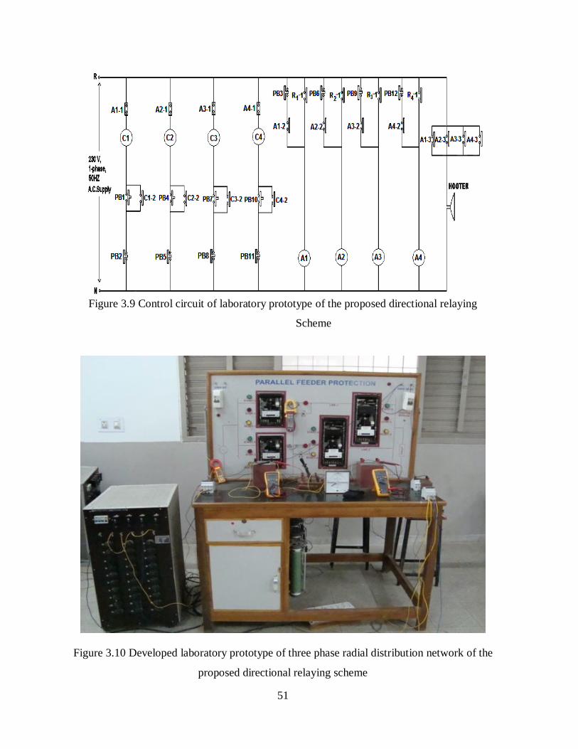
Similarly, the same procedure is followed for a fault in section-2 (Figure 3.8). Figure 3.10
shows pictorial view of the developed laboratory prototype for three phase radial distribution
network having two sections.
51
Figure 3.9 Control circuit of laboratory prototype of the proposed directional relaying
Scheme
Figure 3.10 Developed laboratory prototype of three phase radial distribution network of the
proposed directional relaying scheme
52
3.5 SOFTWARE SELECTION FOR MODELING OF THE SYSTEM
The software selected for this purpose is PSCAD (Power System Computer Aided
Design) which uses EMTDC (Electromagnetic Transient in DC System) [106]. This software
has the capability of performing interpolation between minimum time steps. It uses
trapezoidal methods for solving numerical integrations and differential equations. It manifests
the continuous oscillation of the node voltage (branch current) with changing direction in
every time step, which is not a representative of any electrical behavior of the network. It
enables the user to schematically construct a circuit, run a simulation, analyse the results, and
manage the data in a completely integrated, graphical environment. Online plotting functions,
controls, and meters are also included so that the user can alter system parameters during a
simulation run and view the results directly. It comes with a library of pre-programmed and
tested models, ranging from simple passive elements and control functions to more complex
models, such as electric machines, FACTS (flexible AC transmission systems) devices,
transmission lines, relays, cables and many power system devices. If a particular model does
not exist, it provides the flexibility of building custom models, either by assembling those
graphically using existing models, or by utilizing an intuitively designed design editor.
3.6 MODELING AND SIMULATION OF RADIAL DISTRIBUTION SYSTEMS IN
PRESENCE OF DG USING PSCAD AND LABORATORY PROTOTYPE
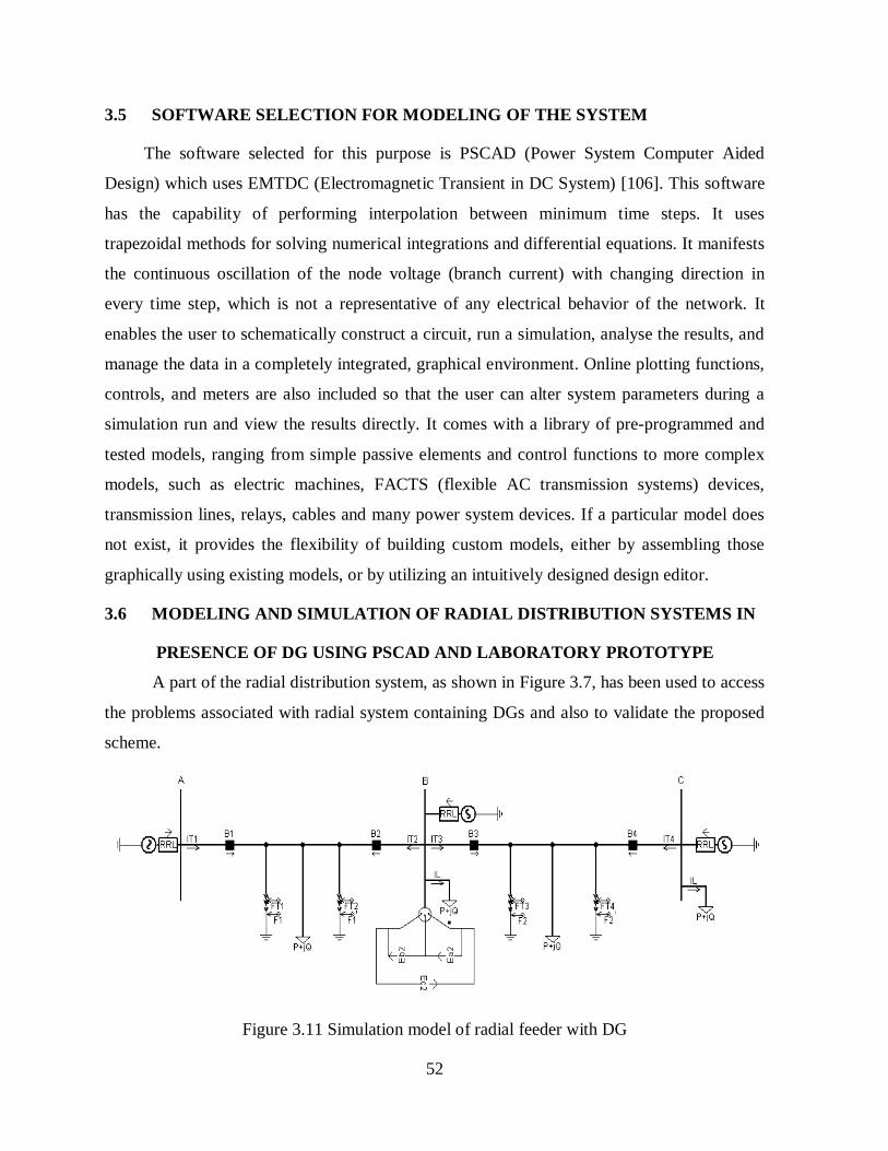
A part of the radial distribution system, as shown in Figure 3.7, has been used to access
the problems associated with radial system containing DGs and also to validate the proposed
scheme.
Figure 3.11 Simulation model of radial feeder with DG
53
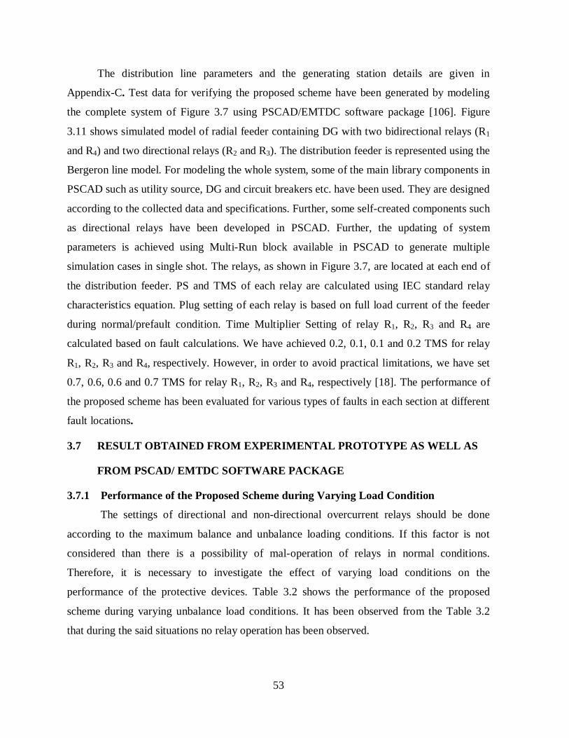
The distribution line parameters and the generating station details are given in
Appendix-C. Test data for verifying the proposed scheme have been generated by modeling
the complete system of Figure 3.7 using PSCAD/EMTDC software package [106]. Figure
3.11 shows simulated model of radial feeder containing DG with two bidirectional relays (R1
and R4) and two directional relays (R2 and R3). The distribution feeder is represented using the
Bergeron line model. For modeling the whole system, some of the main library components in
PSCAD such as utility source, DG and circuit breakers etc. have been used. They are designed
according to the collected data and specifications. Further, some self-created components such
as directional relays have been developed in PSCAD. Further, the updating of system
parameters is achieved using Multi-Run block available in PSCAD to generate multiple
simulation cases in single shot. The relays, as shown in Figure 3.7, are located at each end of
the distribution feeder. PS and TMS of each relay are calculated using IEC standard relay
characteristics equation. Plug setting of each relay is based on full load current of the feeder
during normal/prefault condition. Time Multiplier Setting of relay R1, R2, R3 and R4 are
calculated based on fault calculations. We have achieved 0.2, 0.1, 0.1 and 0.2 TMS for relay
R1, R2, R3 and R4, respectively. However, in order to avoid practical limitations, we have set
0.7, 0.6, 0.6 and 0.7 TMS for relay R1, R2, R3 and R4, respectively [18]. The performance of
the proposed scheme has been evaluated for various types of faults in each section at different
fault locations.
3.7 RESULT OBTAINED FROM EXPERIMENTAL PROTOTYPE AS WELL AS
FROM PSCAD/ EMTDC SOFTWARE PACKAGE
3.7.1 Performance of the Proposed Scheme during Varying Load Condition
The settings of directional and non-directional overcurrent relays should be done
according to the maximum balance and unbalance loading conditions. If this factor is not
considered than there is a possibility of mal-operation of relays in normal conditions.
Therefore, it is necessary to investigate the effect of varying load conditions on the
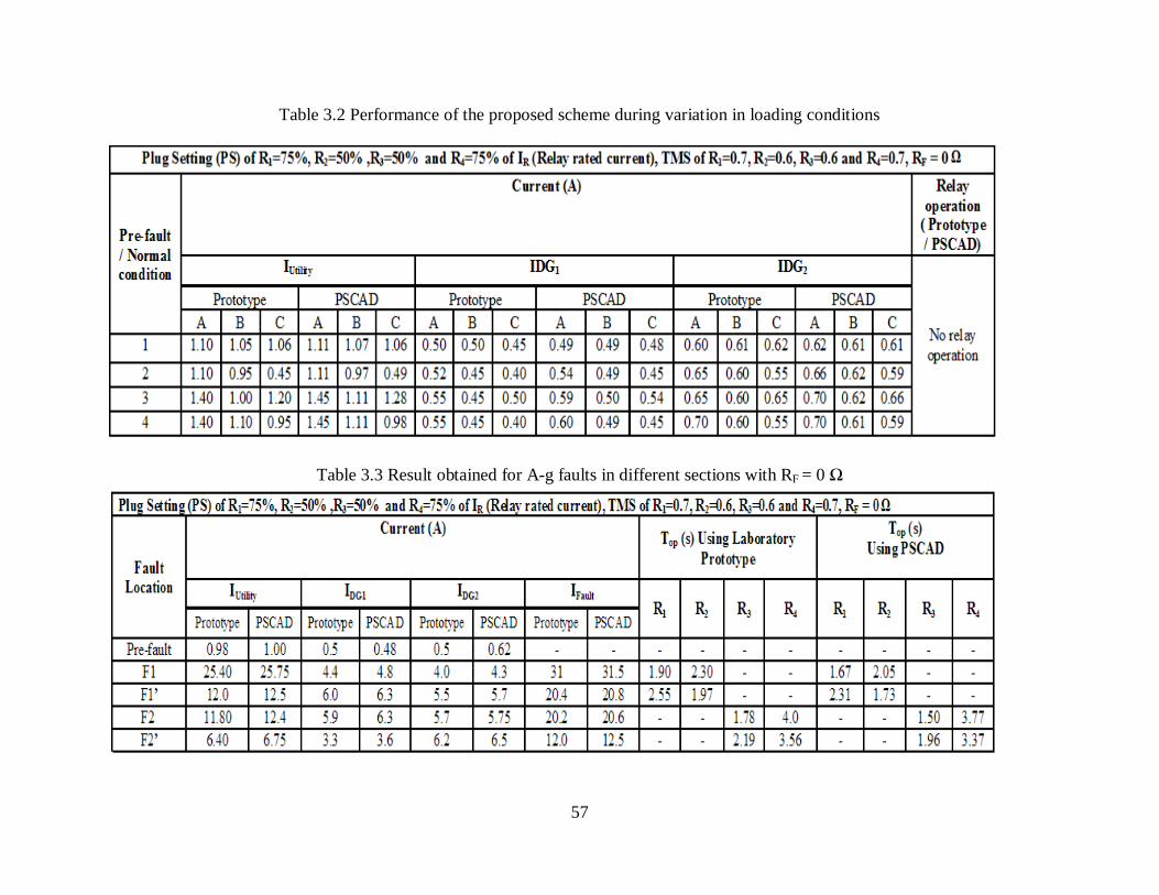
performance of the protective devices. Table 3.2 shows the performance of the proposed
scheme during varying unbalance load conditions. It has been observed from the Table 3.2
that during the said situations no relay operation has been observed.
54
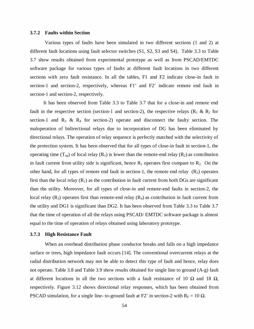
3.7.2 Faults within Section
Various types of faults have been simulated in two different sections (1 and 2) at
different fault locations using fault selector switches (S1, S2, S3 and S4). Table 3.3 to Table
3.7 show results obtained from experimental prototype as well as from PSCAD/EMTDC
software package for various types of faults at different fault locations in two different
sections with zero fault resistance. In all the tables, F1 and F2 indicate close-in fault in
section-1 and section-2, respectively, whereas F1’ and F2’ indicate remote end fault in
section-1 and section-2, respectively.
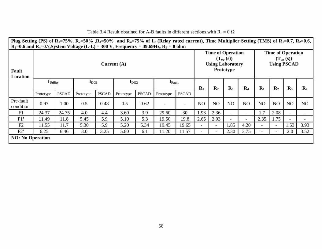
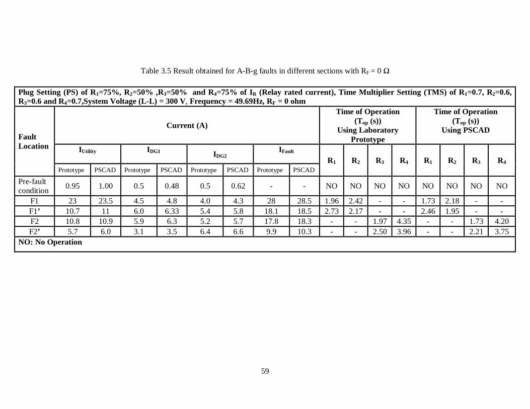
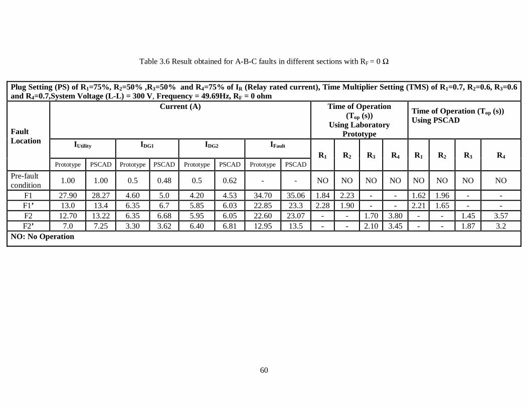
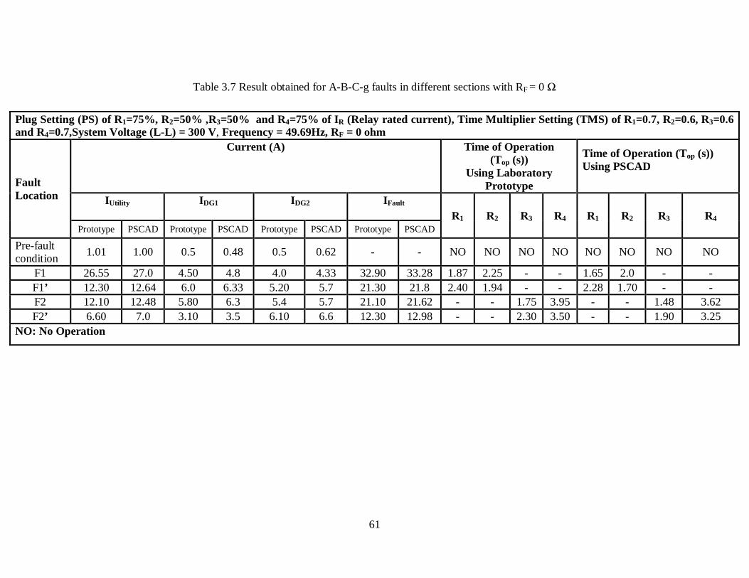
It has been observed from Table 3.3 to Table 3.7 that for a close-in and remote end
fault in the respective section (section-1 and section-2), the respective relays (R1 & R2 for
section-1 and R3 & R4 for section-2) operate and disconnect the faulty section. The
maloperation of bidirectional relays due to incorporation of DG has been eliminated by
directional relays. The operation of relay sequence is perfectly matched with the selectivity of
the protection system. It has been observed that for all types of close-in fault in section-1, the
operating time (Top) of local relay (R1) is lower than the remote-end relay (R2) as contribution
in fault current from utility side is significant, hence R1 operates first compare to R2. On the
other hand, for all types of remote end fault in section-1, the remote end relay (R2) operates
first than the local relay (R1) as the contribution in fault current from both DGs are significant
than the utility. Moreover, for all types of close-in and remote-end faults in section-2, the
local relay (R3) operates first than remote-end relay (R4) as contribution in fault current from
the utility and DG1 is significant than DG2. It has been observed from Table 3.3 to Table 3.7
that the time of operation of all the relays using PSCAD/ EMTDC software package is almost
equal to the time of operation of relays obtained using laboratory prototype.
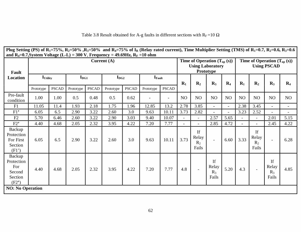
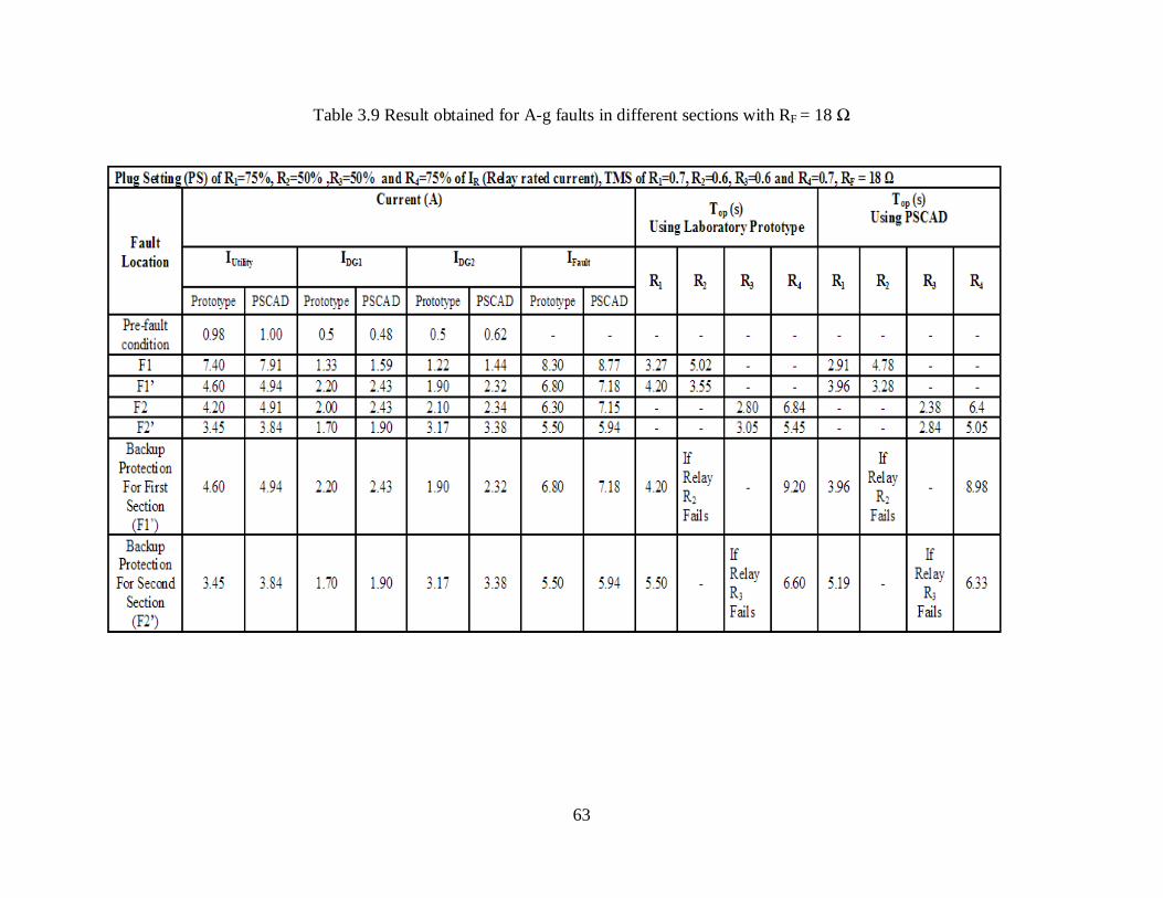
3.7.3 High Resistance Fault
When an overhead distribution phase conductor breaks and falls on a high impedance
surface or trees, high impedance fault occurs [14]. The conventional overcurrent relays at the
radial distribution network may not be able to detect this type of fault and hence, relay does
not operate. Table 3.8 and Table 3.9 show results obtained for single line to ground (A-g) fault
at different locations in all the two sections with a fault resistance of 10 Ω and 18 Ω,
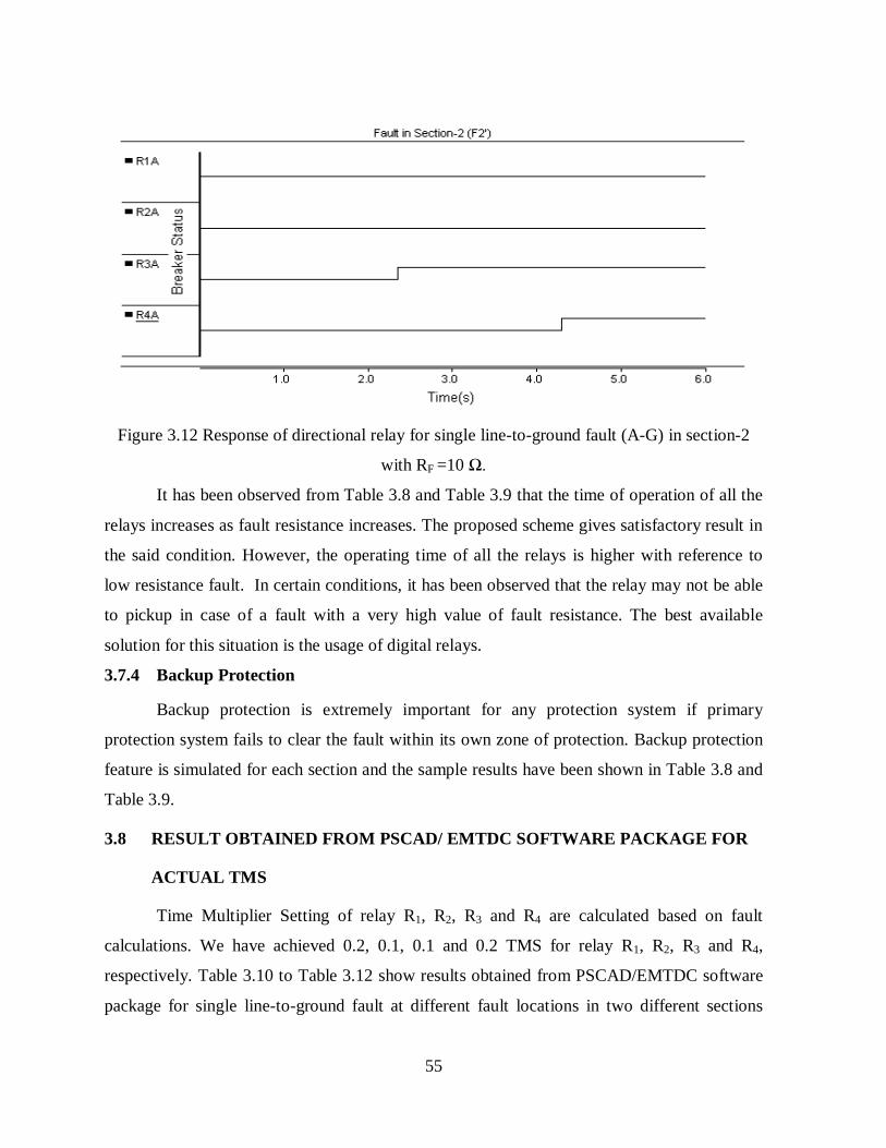
respectively. Figure 3.12 shows directional relay responses, which has been obtained from
PSCAD simulation, for a single line- to-ground fault at F2’ in section-2 with RF = 10 Ω.
55
Figure 3.12 Response of directional relay for single line-to-ground fault (A-G) in section-2
with RF =10 Ω.
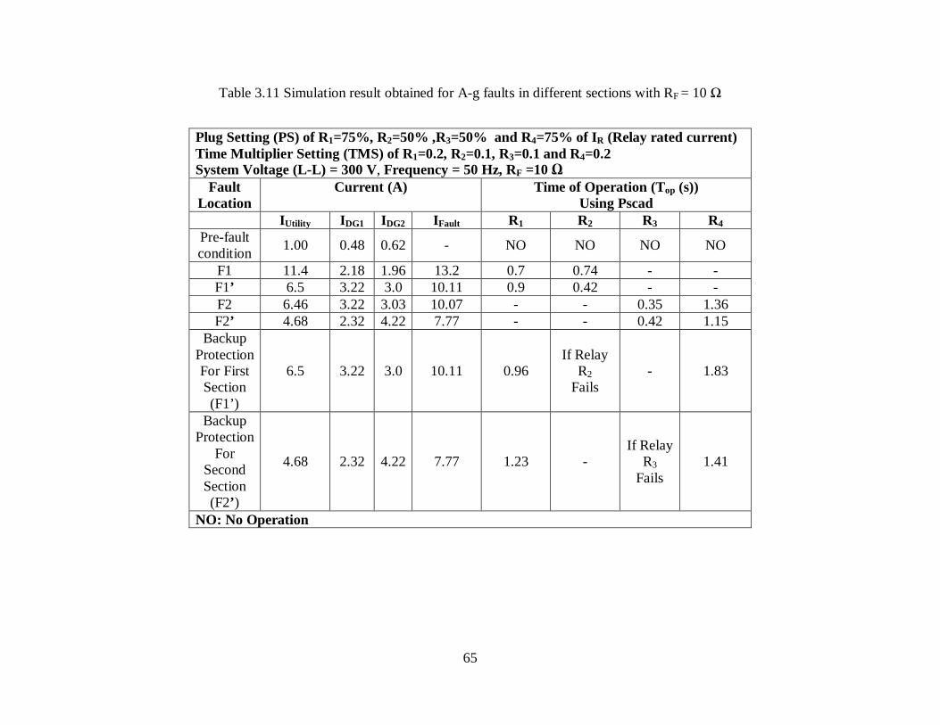
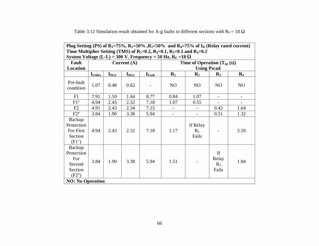
It has been observed from Table 3.8 and Table 3.9 that the time of operation of all the
relays increases as fault resistance increases. The proposed scheme gives satisfactory result in
the said condition. However, the operating time of all the relays is higher with reference to
low resistance fault. In certain conditions, it has been observed that the relay may not be able
to pickup in case of a fault with a very high value of fault resistance. The best available
solution for this situation is the usage of digital relays.
3.7.4 Backup Protection
Backup protection is extremely important for any protection system if primary
protection system fails to clear the fault within its own zone of protection. Backup protection
feature is simulated for each section and the sample results have been shown in Table 3.8 and
Table 3.9.
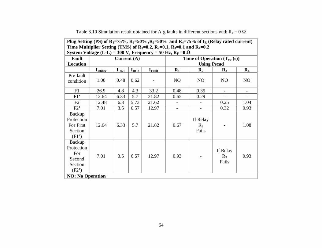
3.8 RESULT OBTAINED FROM PSCAD/ EMTDC SOFTWARE PACKAGE FOR
ACTUAL TMS
Time Multiplier Setting of relay R1, R2, R3 and R4 are calculated based on fault
calculations. We have achieved 0.2, 0.1, 0.1 and 0.2 TMS for relay R1, R2, R3 and R4, respectively. Table 3.10 to Table 3.12 show results obtained from PSCAD/EMTDC software
package for single line-to-ground fault at different fault locations in two different sections
56
with a fault resistance of 0 Ω, 10 Ω and 18 Ω, respectively. The performance of the proposed
scheme has been evaluated for various types of faults in each section at different fault
locations. It has been observed from Table 3.10 to Table 3.12 that the time of operation of all
the relays decreases as TMS of all relays are less compare to results obtained from laboratory
prototype with higher TMS.
Moreover, the proposed scheme also provides back-up protection if primary protection
system fails to operate for a fault within its own zone. Backup protection feature is simulated
for each section and the sample results have been shown in Table 3.10 to Table 3.12.
57
Table 3.2 Performance of the proposed scheme during variation in loading conditions
Table 3.3 Result obtained for A-g faults in different sections with RF = 0 Ω
58
Table 3.4 Result obtained for A-B faults in different sections with RF = 0 Ω
Plug Setting (PS) of R1=75%, R2=50% ,R3=50% and R4=75% of IR (Relay rated current), Time Multiplier Setting (TMS) of R1=0.7, R2=0.6, R3=0.6 and R4=0.7,System Voltage (L-L) = 300 V, Frequency = 49.69Hz, RF = 0 ohm
Fault Location
Current (A)
Time of Operation (Top (s))
Using Laboratory Prototype
Time of Operation (Top (s))
Using PSCAD
IUtility
IDG1
IDG2 IFault
R1 R2 R3 R4 R1 R2 R3 R4 Prototype PSCAD Prototype PSCAD Prototype PSCAD Prototype PSCAD
Pre-fault condition 0.97 1.00 0.5 0.48 0.5 0.62 - - NO NO NO NO NO NO NO NO
F1 24.37 24.75 4.0 4.4 3.60 3.9 29.60 30 1.93 2.36 - - 1.7 2.08 - - F1’ 11.49 11.8 5.45 5.9 5.10 5.3 19.50 19.8 2.65 2.03 - - 2.35 1.75 - -
F2 11.55 11.7 5.30 5.9 5.20 5.34 19.45 19.65 - - 1.85 4.20 - - 1.53 3.93 F2’ 6.25 6.46 3.0 3.25 5.80 6.1 11.20 11.57 - - 2.30 3.75 - - 2.0 3.52
NO: No Operation
59
Table 3.5 Result obtained for A-B-g faults in different sections with RF = 0 Ω
Plug Setting (PS) of R1=75%, R2=50% ,R3=50% and R4=75% of IR (Relay rated current), Time Multiplier Setting (TMS) of R1=0.7, R2=0.6, R3=0.6 and R4=0.7,System Voltage (L-L) = 300 V, Frequency = 49.69Hz, RF = 0 ohm
Fault Location
Current (A)
Time of Operation (Top (s))
Using Laboratory Prototype
Time of Operation (Top (s))
Using PSCAD
IUtility
IDG1 IDG2 IFault
R1 R2 R3 R4 R1 R2 R3 R4 Prototype PSCAD Prototype PSCAD Prototype PSCAD Prototype PSCAD
Pre-fault condition 0.95 1.00 0.5 0.48 0.5 0.62 - - NO NO NO NO NO NO NO NO
F1 23 23.5 4.5 4.8 4.0 4.3 28 28.5 1.96 2.42 - - 1.73 2.18 - - F1’ 10.7 11 6.0 6.33 5.4 5.8 18.1 18.5 2.73 2.17 - - 2.46 1.95 - -
F2 10.8 10.9 5.9 6.3 5.2 5.7 17.8 18.3 - - 1.97 4.35 - - 1.73 4.20 F2’ 5.7 6.0 3.1 3.5 6.4 6.6 9.9 10.3 - - 2.50 3.96 - - 2.21 3.75
NO: No Operation
60
Table 3.6 Result obtained for A-B-C faults in different sections with RF = 0 Ω
Plug Setting (PS) of R1=75%, R2=50% ,R3=50% and R4=75% of IR (Relay rated current), Time Multiplier Setting (TMS) of R1=0.7, R2=0.6, R3=0.6 and R4=0.7,System Voltage (L-L) = 300 V, Frequency = 49.69Hz, RF = 0 ohm
Fault Location
Current (A) Time of Operation (Top (s))
Using Laboratory Prototype
Time of Operation (Top (s)) Using PSCAD
IUtility
IDG1
IDG2 IFault
R1 R2 R3 R4 R1 R2 R3 R4 Prototype PSCAD Prototype PSCAD Prototype PSCAD Prototype PSCAD
Pre-fault condition 1.00 1.00 0.5 0.48 0.5 0.62 - - NO NO NO NO NO NO NO NO
F1 27.90 28.27 4.60 5.0 4.20 4.53 34.70 35.06 1.84 2.23 - - 1.62 1.96 - - F1’ 13.0 13.4 6.35 6.7 5.85 6.03 22.85 23.3 2.28 1.90 - - 2.21 1.65 - - F2 12.70 13.22 6.35 6.68 5.95 6.05 22.60 23.07 - - 1.70 3.80 - - 1.45 3.57 F2’ 7.0 7.25 3.30 3.62 6.40 6.81 12.95 13.5 - - 2.10 3.45 - - 1.87 3.2
NO: No Operation
61
Table 3.7 Result obtained for A-B-C-g faults in different sections with RF = 0 Ω
Plug Setting (PS) of R1=75%, R2=50% ,R3=50% and R4=75% of IR (Relay rated current), Time Multiplier Setting (TMS) of R1=0.7, R2=0.6, R3=0.6 and R4=0.7,System Voltage (L-L) = 300 V, Frequency = 49.69Hz, RF = 0 ohm
Fault Location
Current (A) Time of Operation (Top (s))
Using Laboratory Prototype
Time of Operation (Top (s)) Using PSCAD
IUtility
IDG1
IDG2 IFault
R1 R2 R3 R4 R1 R2 R3 R4 Prototype PSCAD Prototype PSCAD Prototype PSCAD Prototype PSCAD
Pre-fault condition 1.01 1.00 0.5 0.48 0.5 0.62 - - NO NO NO NO NO NO NO NO
F1 26.55 27.0 4.50 4.8 4.0 4.33 32.90 33.28 1.87 2.25 - - 1.65 2.0 - - F1’ 12.30 12.64 6.0 6.33 5.20 5.7 21.30 21.8 2.40 1.94 - - 2.28 1.70 - - F2 12.10 12.48 5.80 6.3 5.4 5.7 21.10 21.62 - - 1.75 3.95 - - 1.48 3.62 F2’ 6.60 7.0 3.10 3.5 6.10 6.6 12.30 12.98 - - 2.30 3.50 - - 1.90 3.25
NO: No Operation
62
Table 3.8 Result obtained for A-g faults in different sections with RF =10 Ω
Plug Setting (PS) of R1=75%, R2=50% ,R3=50% and R4=75% of IR (Relay rated current), Time Multiplier Setting (TMS) of R1=0.7, R2=0.6, R3=0.6 and R4=0.7,System Voltage (L-L) = 300 V, Frequency = 49.69Hz, RF =10 ohm
Fault Location
Current (A)
Time of Operation (Top (s)) Using Laboratory
Prototype
Time of Operation (Top (s)) Using PSCAD
IUtility
IDG1
IDG2 IFault
R1 R2 R3 R4 R1 R2 R3 R4 Prototype PSCAD Prototype PSCAD Prototype PSCAD Prototype PSCAD
Pre-fault condition 1.00 1.00 0.5 0.48 0.5 0.62 - - NO NO NO NO NO NO NO NO
F1 11.05 11.4 1.93 2.18 1.75 1.96 12.85 13.2 2.78 3.85 - - 2.38 3.45 - - F1’ 6.05 6.5 2.90 3.22 2.60 3.0 9.63 10.11 3.73 2.82 - - 3.23 2.52 - - F2 5.70 6.46 2.60 3.22 2.90 3.03 9.40 10.07 - - 2.57 5.65 - - 2.01 5.15 F2’ 4.40 4.68 2.05 2.32 3.95 4.22 7.20 7.77 - - 2.85 4.72 - - 2.45 4.22
Backup Protection For First Section (F1’)
6.05 6.5 2.90 3.22 2.60 3.0 9.63 10.11 3.73
If Relay
R2 Fails
- 6.60 3.33
If Relay
R2 Fails
- 6.28
Backup Protection
For Second Section (F2’)
4.40 4.68 2.05 2.32 3.95 4.22 7.20 7.77 4.8 -
If Relay
R3 Fails
5.20 4.3 -
If Relay
R3 Fails
4.85
NO: No Operation
63
Table 3.9 Result obtained for A-g faults in different sections with RF = 18 Ω
64
Table 3.10 Simulation result obtained for A-g faults in different sections with RF = 0 Ω
Plug Setting (PS) of R1=75%, R2=50% ,R3=50% and R4=75% of IR (Relay rated current) Time Multiplier Setting (TMS) of R1=0.2, R2=0.1, R3=0.1 and R4=0.2 System Voltage (L-L) = 300 V, Frequency = 50 Hz, RF =0 Ω
Fault Location
Current (A) Time of Operation (Top (s)) Using Pscad
IUtility IDG1 IDG2 IFault R1 R2 R3 R4 Pre-fault condition 1.00 0.48 0.62 - NO NO NO NO
F1 26.9 4.8 4.3 33.2 0.48 0.35 - - F1’ 12.64 6.33 5.7 21.82 0.65 0.29 - - F2 12.48 6.3 5.73 21.62 - - 0.25 1.04 F2’ 7.01 3.5 6.57 12.97 - - 0.32 0.93
Backup Protection For First Section (F1’)
12.64 6.33 5.7 21.82 0.67 If Relay
R2 Fails
- 1.08
Backup Protection
For Second Section (F2’)
7.01 3.5 6.57 12.97 0.93 - If Relay
R3 Fails
0.93
NO: No Operation
65
Table 3.11 Simulation result obtained for A-g faults in different sections with RF = 10 Ω
Plug Setting (PS) of R1=75%, R2=50% ,R3=50% and R4=75% of IR (Relay rated current) Time Multiplier Setting (TMS) of R1=0.2, R2=0.1, R3=0.1 and R4=0.2 System Voltage (L-L) = 300 V, Frequency = 50 Hz, RF =10 Ω
Fault Location
Current (A) Time of Operation (Top (s)) Using Pscad
IUtility IDG1 IDG2 IFault R1 R2 R3 R4 Pre-fault condition 1.00 0.48 0.62 - NO NO NO NO
F1 11.4 2.18 1.96 13.2 0.7 0.74 - - F1’ 6.5 3.22 3.0 10.11 0.9 0.42 - - F2 6.46 3.22 3.03 10.07 - - 0.35 1.36 F2’ 4.68 2.32 4.22 7.77 - - 0.42 1.15
Backup Protection For First Section (F1’)
6.5 3.22 3.0 10.11 0.96 If Relay
R2 Fails
- 1.83
Backup Protection
For Second Section (F2’)
4.68 2.32 4.22 7.77 1.23 - If Relay
R3 Fails
1.41
NO: No Operation
66
Table 3.12 Simulation result obtained for A-g faults in different sections with RF = 18 Ω
Plug Setting (PS) of R1=75%, R2=50% ,R3=50% and R4=75% of IR (Relay rated current) Time Multiplier Setting (TMS) of R1=0.2, R2=0.1, R3=0.1 and R4=0.2 System Voltage (L-L) = 300 V, Frequency = 50 Hz, RF =18 Ω
Fault Location
Current (A) Time of Operation (Top (s)) Using Pscad
IUtility IDG1 IDG2 IFault R1 R2 R3 R4
Pre-fault condition 1.07
0.48
0.62
- NO NO NO NO
F1 7.91 1.59 1.44 8.77 0.84 1.07 - - F1’ 4.94 2.43 2.32 7.18 1.07 0.55 - - F2 4.91 2.43 2.34 7.15 - - 0.42 1.64 F2’ 3.84 1.90 3.38 5.94 - - 0.51 1.32
Backup Protection For First Section (F1’)
4.94 2.43 2.32 7.18 1.17 If Relay
R2 Fails
- 2.59
Backup Protection
For Second Section (F2’)
3.84 1.90 3.38 5.94 1.51 -
If Relay
R3 Fails
1.84
NO: No Operation
67
3.9 MODELING AND SIMULATION OF A LARGE 11 KV RADIAL
DISTRIBUTION SYSTEMS IN THE PRESENCE OF DG USING PSCAD
3.9.1 System Description of a Large 11 kV Radial Distribution Systems in the Presence
of DG
A part of the Indian 11 kV radial distribution system, as shown in Figure 3.7 and
Figure 3.8, has been used to access the problems associated with radial system containing
DGs and also to validate the proposed scheme. The distribution line parameters and the
generating station details are given in Appendix-D. Test data for verifying the proposed
scheme have been generated by modeling the complete system of Figure 3.7 using the
PSCAD/EMTDC software package [106]. The performance of the proposed scheme has been
evaluated for various types of faults in each section at different fault locations. Relay
responses for some special cases such as high resistance fault and backup protection were also
investigated.
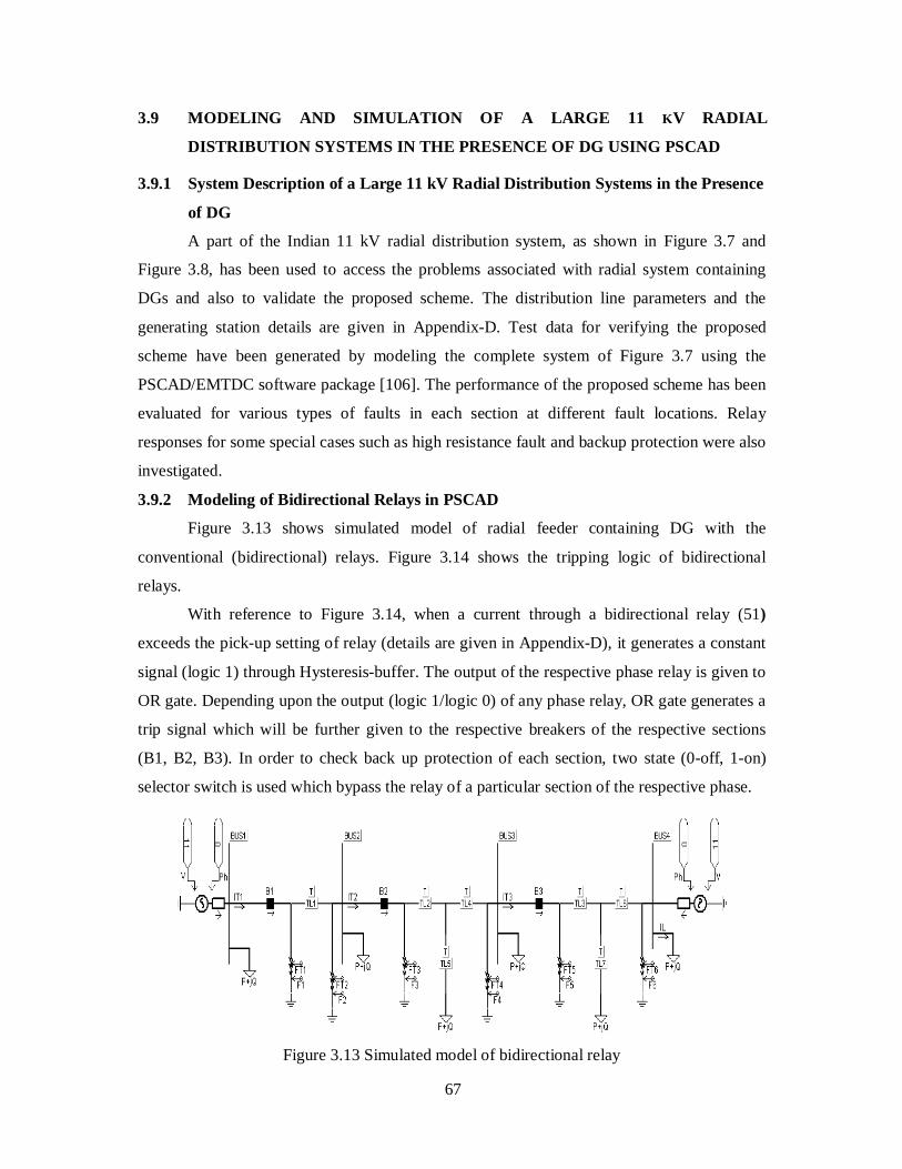
3.9.2 Modeling of Bidirectional Relays in PSCAD
Figure 3.13 shows simulated model of radial feeder containing DG with the
conventional (bidirectional) relays. Figure 3.14 shows the tripping logic of bidirectional
relays.
With reference to Figure 3.14, when a current through a bidirectional relay (51)
exceeds the pick-up setting of relay (details are given in Appendix-D), it generates a constant
signal (logic 1) through Hysteresis-buffer. The output of the respective phase relay is given to
OR gate. Depending upon the output (logic 1/logic 0) of any phase relay, OR gate generates a
trip signal which will be further given to the respective breakers of the respective sections
(B1, B2, B3). In order to check back up protection of each section, two state (0-off, 1-on)
selector switch is used which bypass the relay of a particular section of the respective phase.
Figure 3.13 Simulated model of bidirectional relay
68
Figure 3.14 Tripping logic of bidirectional relay
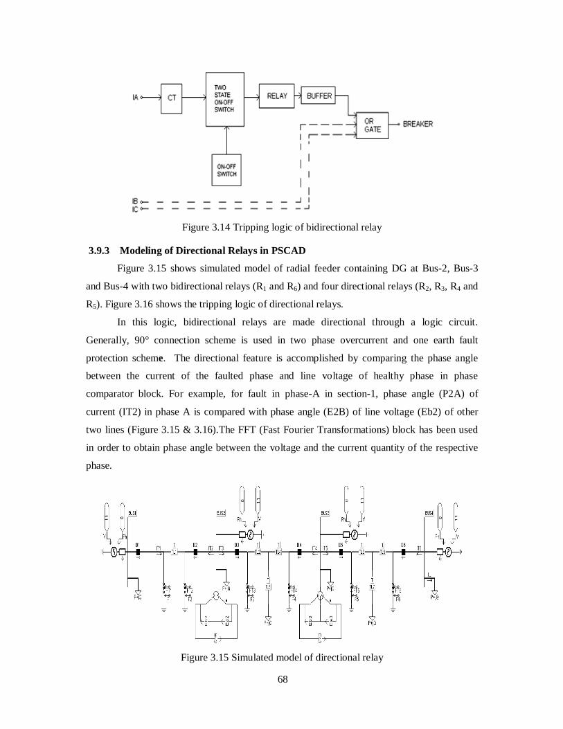
3.9.3 Modeling of Directional Relays in PSCAD
Figure 3.15 shows simulated model of radial feeder containing DG at Bus-2, Bus-3
and Bus-4 with two bidirectional relays (R1 and R6) and four directional relays (R2, R3, R4 and
R5). Figure 3.16 shows the tripping logic of directional relays.
In this logic, bidirectional relays are made directional through a logic circuit.
Generally, 90° connection scheme is used in two phase overcurrent and one earth fault
protection scheme. The directional feature is accomplished by comparing the phase angle
between the current of the faulted phase and line voltage of healthy phase in phase
comparator block. For example, for fault in phase-A in section-1, phase angle (P2A) of
current (IT2) in phase A is compared with phase angle (E2B) of line voltage (Eb2) of other
two lines (Figure 3.15 & 3.16).The FFT (Fast Fourier Transformations) block has been used
in order to obtain phase angle between the voltage and the current quantity of the respective
phase.
Figure 3.15 Simulated model of directional relay
69
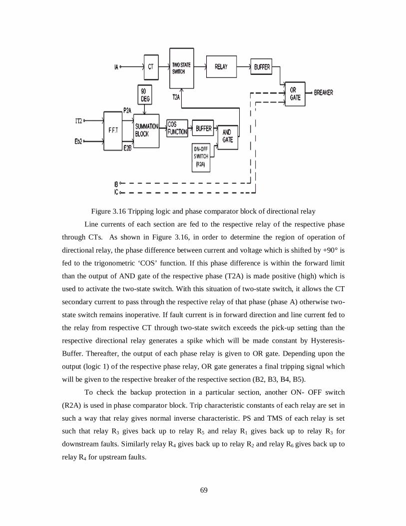
Figure 3.16 Tripping logic and phase comparator block of directional relay
Line currents of each section are fed to the respective relay of the respective phase
through CTs. As shown in Figure 3.16, in order to determine the region of operation of
directional relay, the phase difference between current and voltage which is shifted by +90° is
fed to the trigonometric ‘COS’ function. If this phase difference is within the forward limit
than the output of AND gate of the respective phase (T2A) is made positive (high) which is
used to activate the two-state switch. With this situation of two-state switch, it allows the CT
secondary current to pass through the respective relay of that phase (phase A) otherwise two-
state switch remains inoperative. If fault current is in forward direction and line current fed to
the relay from respective CT through two-state switch exceeds the pick-up setting than the
respective directional relay generates a spike which will be made constant by Hysteresis-
Buffer. Thereafter, the output of each phase relay is given to OR gate. Depending upon the
output (logic 1) of the respective phase relay, OR gate generates a final tripping signal which
will be given to the respective breaker of the respective section (B2, B3, B4, B5).
To check the backup protection in a particular section, another ON- OFF switch
(R2A) is used in phase comparator block. Trip characteristic constants of each relay are set in
such a way that relay gives normal inverse characteristic. PS and TMS of each relay is set
such that relay R3 gives back up to relay R5 and relay R1 gives back up to relay R3 for
downstream faults. Similarly relay R4 gives back up to relay R2 and relay R6 gives back up to
relay R4 for upstream faults.
70
3.10 RESULTS AND DISCUSSION
3.10.1 Bidirectional Relay
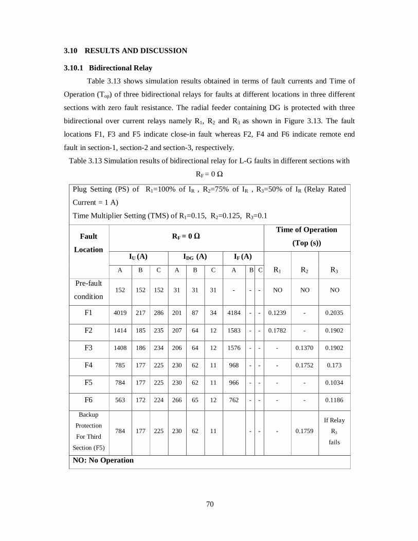
Table 3.13 shows simulation results obtained in terms of fault currents and Time of
Operation (Top) of three bidirectional relays for faults at different locations in three different
sections with zero fault resistance. The radial feeder containing DG is protected with three
bidirectional over current relays namely R1, R2 and R3 as shown in Figure 3.13. The fault
locations F1, F3 and F5 indicate close-in fault whereas F2, F4 and F6 indicate remote end
fault in section-1, section-2 and section-3, respectively.
Table 3.13 Simulation results of bidirectional relay for L-G faults in different sections with
RF = 0 Ω
Plug Setting (PS) of R1=100% of IR , R2=75% of IR , R3=50% of IR (Relay Rated
Current = 1 A)
Time Multiplier Setting (TMS) of R1=0.15, R2=0.125, R3=0.1
Fault
Location
RF = 0 Ω Time of Operation
(Top (s))
IU (A) IDG (A) IF (A)
R1
R2
R3 A B C A B C A B C
Pre-fault
condition 152 152 152 31 31 31 - - - NO NO NO
F1 4019 217 286 201 87 34 4184 - - 0.1239 - 0.2035
F2 1414 185 235 207 64 12 1583 - - 0.1782 - 0.1902
F3 1408 186 234 206 64 12 1576 - - - 0.1370 0.1902
F4 785 177 225 230 62 11 968 - - - 0.1752 0.173
F5 784 177 225 230 62 11 966 - - - - 0.1034
F6 563 172 224 266 65 12 762 - - - - 0.1186
Backup
Protection
For Third
Section (F5)
784 177 225 230 62 11 - - - 0.1759
If Relay
R3
fails
NO: No Operation
71
It has been observed from Table 3.13 that for a close-in and remote end fault in
section-1 (F1 and F2), relay R1 operates first as the contribution of fault current from the
utility side (IU) is significant (strong source). On the other hand, relay R3 operates after some
time delay as the contribution of fault current from DG (weak source) is comparatively lower
than the utility. With the present structure of radial distribution network along with DG, relay
R1 and relay R2 has to trip for a fault in section-1. But, the breaker in section-3 trips
unnecessary due to operation of relay R3. This mal-operation occurs due to the presence of
DG on the other side, which is against the selectivity of the protection system.
Correspondingly, for a close in and remote end fault in section-2 (F3 & F4) relay R2 and relay
R3 operate whereas for a close in and remote end fault in section-3 (F5 & F6), relay R3 and
local protection of DG (Fuse/MCB) operate.
It is to be noted that as the relay is located near the DG, the contribution in fault
current from DG is higher. This would not create a problem in maintaining selectivity as one
can easily disconnect DG when its penetration is low. On the other hand, when penetration of
DG is high and more than one DG is connected at different location, the conventional relay is
not in a position to maintain the proper selectivity. This problem is rectified using the
proposed scheme which works perfectly even during different DG capacities and also during
more than one DG connected at various locations.
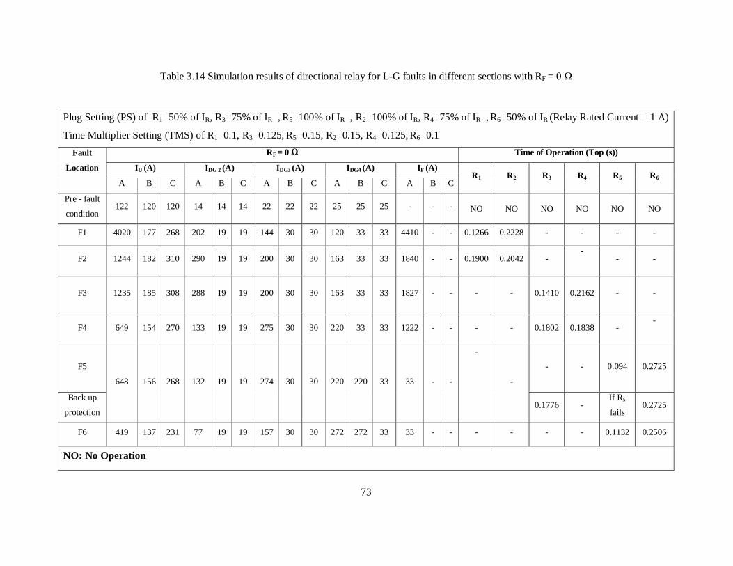
3.10.2 Directional Relay
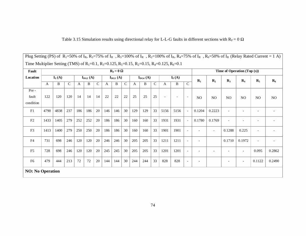
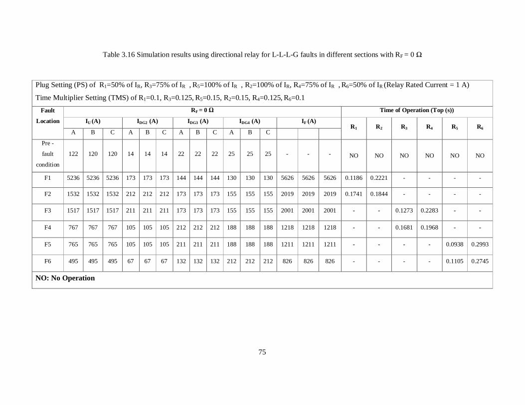
Table 3.14 to Table 3.17 show the simulations results for L-G, L-L-G, L-L-L-G and
L-L faults at different fault locations in three different sections with zero fault resistance. The
radial feeder containing DG is protected with four directional over current relays R2, R3, R4,
R5 and two bidirectional relays R1 and R6 as shown in Figure 3.15.
It has been observed from Table 3.14 to Table 3.17 that for a fault in section-1,
section-2 and section-3 at any locations relay R1 & relay R2, relay R3 & relay R4, relay R5 &
relay R6 operate and disconnect the faulty section, respectively. The maloperation of
bidirectional relays due to incorporation of DG has been eliminated by the proposed scheme.
The operation of relay sequence is perfectly matched with the selectivity of the protection
system. Further, it has been observed from Table 3.14 to Table 3.17 that for all close-in and
remote-end faults in all the three sections, the local end relay (R1, R3 and R5 ) operates first
than the remote-end relay (R2, R4 and R6) as the contribution of fault current from the utility
(IU) is significant (strong source). Figure 3.17 shows directional relay responses, which has
been obtained from PSCAD simulation, for a single line- to-ground fault at F4 in section-2
with RF = 0 Ω.

72
Figure 3.17 Response of directional relay for single line-to-ground fault (A-G) in section-2
with RF = 0 Ω
3.10.3 Backup Protection
Backup protection is extremely important for any protection system if primary
protection system fails to clear the fault within its own zone of protection. Backup protection
feature is simulated for section-3 and the sample result has been shown in Table 3.14.
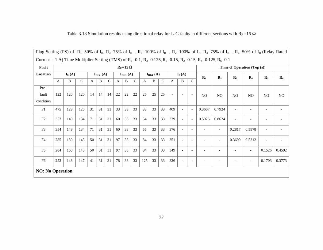
3.10.4 High Resistance Fault
When an overhead distribution phase conductor breaks and falls on a high impedance
surface or trees, high impedance fault occurs [14]. The conventional overcurrent relays at the
radial distribution network may not be able to detect this type of fault and hence, relay does
not operate. To analyze this condition, a case study has been set up and a single line-to-
ground fault with a fault resistance equal to 15 has been simulated. However, in practice,
this value may exceed 30 Ω. Table 3.18 shows the simulation results for L-G faults at
different locations in three different sections with a fault resistance of 15 Ω. It has been
observed from Table 3.18 that for a fault in any section, the primary protection relay of that
section operates first and clears the fault within its own zone. Though, a slower relay
performance is achieved, the proposed scheme operates successfully.
73
Table 3.14 Simulation results of directional relay for L-G faults in different sections with RF = 0 Ω
Plug Setting (PS) of R1=50% of IR, R3=75% of IR , R5=100% of IR , R2=100% of IR, R4=75% of IR , R6=50% of IR (Relay Rated Current = 1 A)
Time Multiplier Setting (TMS) of R1=0.1, R3=0.125, R5=0.15, R2=0.15, R4=0.125, R6=0.1
Fault
Location
RF = 0 Ω Time of Operation (Top (s))
IU (A) IDG 2 (A) IDG3 (A) IDG4 (A) IF (A) R1 R2 R3 R4 R5 R6
A B C A B C A B C A B C A B C
Pre - fault
condition 122 120 120 14 14 14 22 22 22 25 25 25 - - - NO NO NO NO NO NO
F1 4020 177 268 202 19 19 144 30 30 120 33 33 4410 - - 0.1266 0.2228 - - - -
F2 1244 182 310 290 19 19 200 30 30 163 33 33 1840 - - 0.1900 0.2042 - -
- -
F3 1235 185 308 288 19 19 200 30 30 163 33 33 1827 - - - - 0.1410 0.2162 - -
F4 649 154 270 133 19 19 275 30 30 220 33 33 1222 - - - - 0.1802 0.1838 - -
F5
648 156 268 132 19 19 274 30 30 220 220 33 33 - -
-
-
- - 0.094 0.2725
Back up
protection 0.1776 -
If R5
fails 0.2725
F6 419 137 231 77 19 19 157 30 30 272 272 33 33 - - - - - - 0.1132 0.2506
NO: No Operation
74
Table 3.15 Simulation results using directional relay for L-L-G faults in different sections with RF = 0 Ω
Plug Setting (PS) of R1=50% of IR, R3=75% of IR , R5=100% of IR , R2=100% of IR, R4=75% of IR , R6=50% of IR (Relay Rated Current = 1 A)
Time Multiplier Setting (TMS) of R1=0.1, R3=0.125, R5=0.15, R2=0.15, R4=0.125, R6=0.1
Fault
Location
RF = 0 Ω Time of Operation (Top (s))
IU (A) IDG2 (A) IDG3 (A) IDG4 (A) IF (A) R1 R2 R3 R4 R5 R6
A B C A B C A B C A B C A B C
Pre -
fault
condition
122 120 120 14 14 14 22 22 22 25 25 25 - - - NO NO NO NO NO NO
F1 4790 4838 237 186 186 20 146 146 30 129 129 33 5156 5156 - 0.1204 0.2223 - - - -
F2 1433 1405 279 252 252 20 186 186 30 160 160 33 1931 1931 - 0.1780 0.1769 - - - -
F3 1413 1400 279 250 250 20 186 186 30 160 160 33 1901 1901 - - - 0.1288 0.225 - -
F4 731 698 246 120 120 20 246 246 30 205 205 33 1211 1211 - - 0.1710 0.1972 - -
F5 728 698 246 120 120 20 245 245 30 205 205 33 1201 1201 - - - - - 0.095 0.2862
F6 479 444 213 72 72 20 144 144 30 244 244 33 828 828 - - - - 0.1122 0.2490
NO: No Operation
75
Table 3.16 Simulation results using directional relay for L-L-L-G faults in different sections with RF = 0 Ω
Plug Setting (PS) of R1=50% of IR, R3=75% of IR , R5=100% of IR , R2=100% of IR, R4=75% of IR , R6=50% of IR (Relay Rated Current = 1 A)
Time Multiplier Setting (TMS) of R1=0.1, R3=0.125, R5=0.15, R2=0.15, R4=0.125, R6=0.1
Fault
Location
RF = 0 Ω Time of Operation (Top (s))
IU (A) IDG2 (A) IDG3 (A) IDG4 (A) IF (A) R1 R2 R3 R4 R5 R6
A B C A B C A B C A B C
Pre -
fault
condition
122 120 120 14 14 14 22 22 22 25 25 25 - - - NO NO NO NO NO NO
F1 5236 5236 5236 173 173 173 144 144 144 130 130 130 5626 5626 5626 0.1186 0.2221 - - - -
F2 1532 1532 1532 212 212 212 173 173 173 155 155 155 2019 2019 2019 0.1741 0.1844 - - - -
F3 1517 1517 1517 211 211 211 173 173 173 155 155 155 2001 2001 2001 - - 0.1273 0.2283 - -
F4 767 767 767 105 105 105 212 212 212 188 188 188 1218 1218 1218 - - 0.1681 0.1968 - -
F5 765 765 765 105 105 105 211 211 211 188 188 188 1211 1211 1211 - - - - 0.0938 0.2993
F6 495 495 495 67 67 67 132 132 132 212 212 212 826 826 826 - - - - 0.1105 0.2745
NO: No Operation

76
Table 3.17 Simulation results using directional relay for L-L faults in different sections with RF = 0 Ω
Plug Setting (PS) of R1=50% of IR, R3=75% of IR , R5=100% of IR , R2=100% of IR, R4=75% of IR , R6=50% of IR (Relay Rated Current = 1 A)
Time Multiplier Setting (TMS) of R1=0.1, R3=0.125, R5=0.15, R2=0.15, R4=0.125, R6=0.1
Fault
Location
RF = 0 Ω Time of Operation (Top (s))
IU (A) IDG2 (A) IDG3 (A) IDG4 (A) IF (A) R1 R2 R3 R4 R5 R6
A B C A B C A B C A B C A B C
Pre -
fault
condition
122 120 120 14 14 14 22 22 22 25 25 25 - - - NO NO NO NO NO NO
F1 4593 4477 164 156 156 20 134 134 30 123 123 33 4873 4873 - 0.1207 0.2630 - - - -
F2 1381 1271 159 190 190 20 159 159 30 145 145 33 1749 1749 - 0.1824 0.2152 - - - -
F3 1365 1262 159 189 189 20 159 159 30 145 145 33 1733 1733 - - - 0.1313 0.2560 - -
F4 715 614 154 97 97 20 193 193 30 174 174 33 1055 1055 - - - 0.1757 0.2186 - -
F5 711 613 154 97 97 20 193 193 30 174 174 33 1049 1049 - - - - - 0.097 0.3233
F6 478 385 152 64 64 20 124 124 30 194 194 33 715 715 - - - - - 0.1158 0.2953
NO: No Operation
77
Table 3.18 Simulation results using directional relay for L-G faults in different sections with RF =15 Ω
Plug Setting (PS) of R1=50% of IR, R3=75% of IR , R5=100% of IR , R2=100% of IR, R4=75% of IR , R6=50% of IR (Relay Rated
Current = 1 A) Time Multiplier Setting (TMS) of R1=0.1, R3=0.125, R5=0.15, R2=0.15, R4=0.125, R6=0.1
Fault
Location
RF =15 Ω Time of Operation (Top (s))
IU (A) IDG2 (A) IDG3 (A) IDG4 (A) IF (A) R1 R2 R3 R4 R5 R6
A B C A B C A B C A B C A B C
Pre -
fault
condition
122 120 120 14 14 14 22 22 22 25 25 25 - - - NO NO NO NO NO NO
F1 475 129 120 31 31 31 33 33 33 33 33 33 409 - - 0.3607 0.7924 - - - -
F2 357 149 134 71 31 31 60 33 33 54 33 33 379 - - 0.5026 0.8624 - - - -
F3 354 149 134 71 31 31 60 33 33 55 33 33 376 - - - - 0.2817 0.5978 - -
F4 285 150 143 50 31 31 97 33 33 84 33 33 351 - - - - 0.3699 0.5312 - -
F5 284 150 143 50 31 31 97 33 33 84 33 33 349 - - - - - - 0.1526 0.4592
F6 252 148 147 41 31 31 78 33 33 125 33 33 326 - - - - - - 0.1703 0.3773
NO: No Operation
78
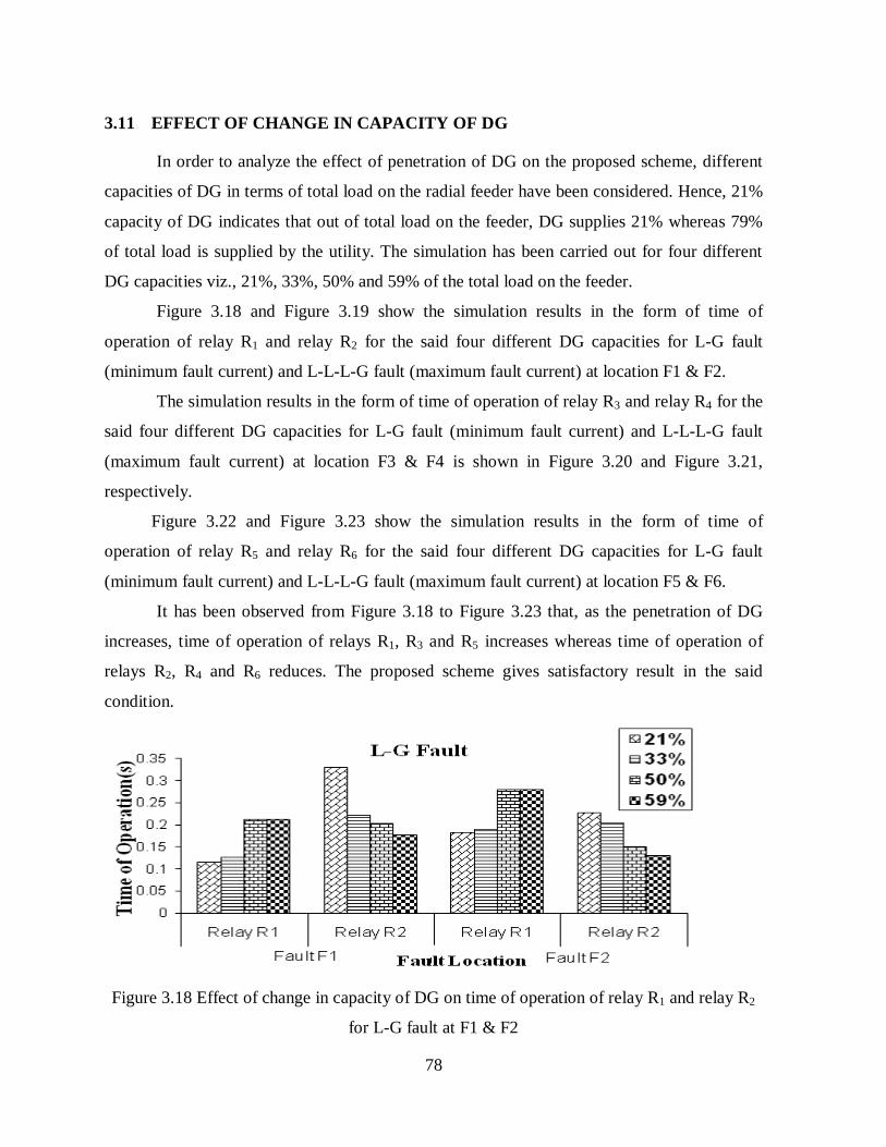
3.11 EFFECT OF CHANGE IN CAPACITY OF DG
In order to analyze the effect of penetration of DG on the proposed scheme, different
capacities of DG in terms of total load on the radial feeder have been considered. Hence, 21%
capacity of DG indicates that out of total load on the feeder, DG supplies 21% whereas 79%
of total load is supplied by the utility. The simulation has been carried out for four different
DG capacities viz., 21%, 33%, 50% and 59% of the total load on the feeder.
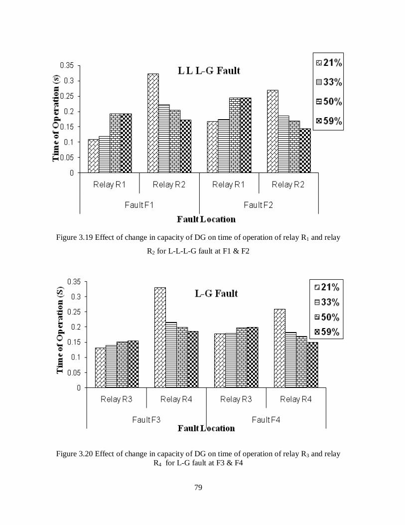
Figure 3.18 and Figure 3.19 show the simulation results in the form of time of
operation of relay R1 and relay R2 for the said four different DG capacities for L-G fault
(minimum fault current) and L-L-L-G fault (maximum fault current) at location F1 & F2.
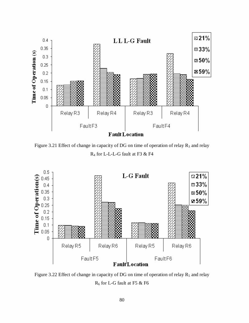
The simulation results in the form of time of operation of relay R3 and relay R4 for the
said four different DG capacities for L-G fault (minimum fault current) and L-L-L-G fault
(maximum fault current) at location F3 & F4 is shown in Figure 3.20 and Figure 3.21,
respectively.
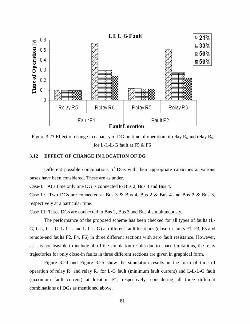
Figure 3.22 and Figure 3.23 show the simulation results in the form of time of
operation of relay R5 and relay R6 for the said four different DG capacities for L-G fault
(minimum fault current) and L-L-L-G fault (maximum fault current) at location F5 & F6.
It has been observed from Figure 3.18 to Figure 3.23 that, as the penetration of DG
increases, time of operation of relays R1, R3 and R5 increases whereas time of operation of
relays R2, R4 and R6 reduces. The proposed scheme gives satisfactory result in the said
condition.
Figure 3.18 Effect of change in capacity of DG on time of operation of relay R1 and relay R2
for L-G fault at F1 & F2
79
Figure 3.19 Effect of change in capacity of DG on time of operation of relay R1 and relay
R2 for L-L-L-G fault at F1 & F2
Figure 3.20 Effect of change in capacity of DG on time of operation of relay R3 and relay R4 for L-G fault at F3 & F4
80
Figure 3.21 Effect of change in capacity of DG on time of operation of relay R3 and relay
R4 for L-L-L-G fault at F3 & F4
Figure 3.22 Effect of change in capacity of DG on time of operation of relay R5 and relay
R6 for L-G fault at F5 & F6
81
Figure 3.23 Effect of change in capacity of DG on time of operation of relay R5 and relay R6
for L-L-L-G fault at F5 & F6
3.12 EFFECT OF CHANGE IN LOCATION OF DG
Different possible combinations of DGs with their appropriate capacities at various
buses have been considered. These are as under.
Case-I: At a time only one DG is connected to Bus 2, Bus 3 and Bus 4.
Case-II: Two DGs are connected at Bus 3 & Bus 4, Bus 2 & Bus 4 and Bus 2 & Bus 3,
respectively at a particular time.
Case-III: Three DGs are connected to Bus 2, Bus 3 and Bus 4 simultaneously.
The performance of the proposed scheme has been checked for all types of faults (L-
G, L-L, L-L-G, L-L-L and L-L-L-G) at different fault locations (close-in faults F1, F3, F5 and
remote-end faults F2, F4, F6) in three different sections with zero fault resistance. However,
as it is not feasible to include all of the simulation results due to space limitations, the relay
trajectories for only close-in faults in three different sections are given in graphical form.
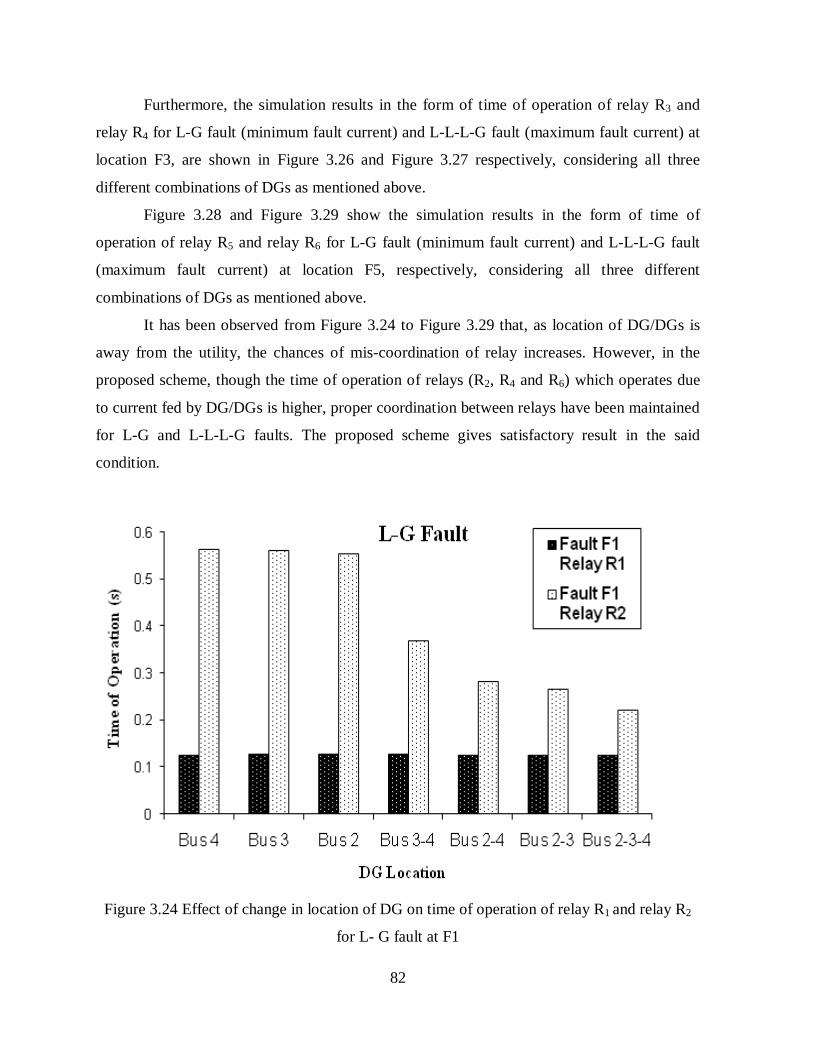
Figure 3.24 and Figure 3.25 show the simulation results in the form of time of
operation of relay R1 and relay R2 for L-G fault (minimum fault current) and L-L-L-G fault
(maximum fault current) at location F1, respectively, considering all three different
combinations of DGs as mentioned above.
82
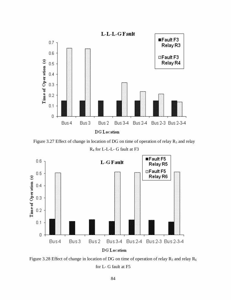
Furthermore, the simulation results in the form of time of operation of relay R3 and
relay R4 for L-G fault (minimum fault current) and L-L-L-G fault (maximum fault current) at
location F3, are shown in Figure 3.26 and Figure 3.27 respectively, considering all three
different combinations of DGs as mentioned above.
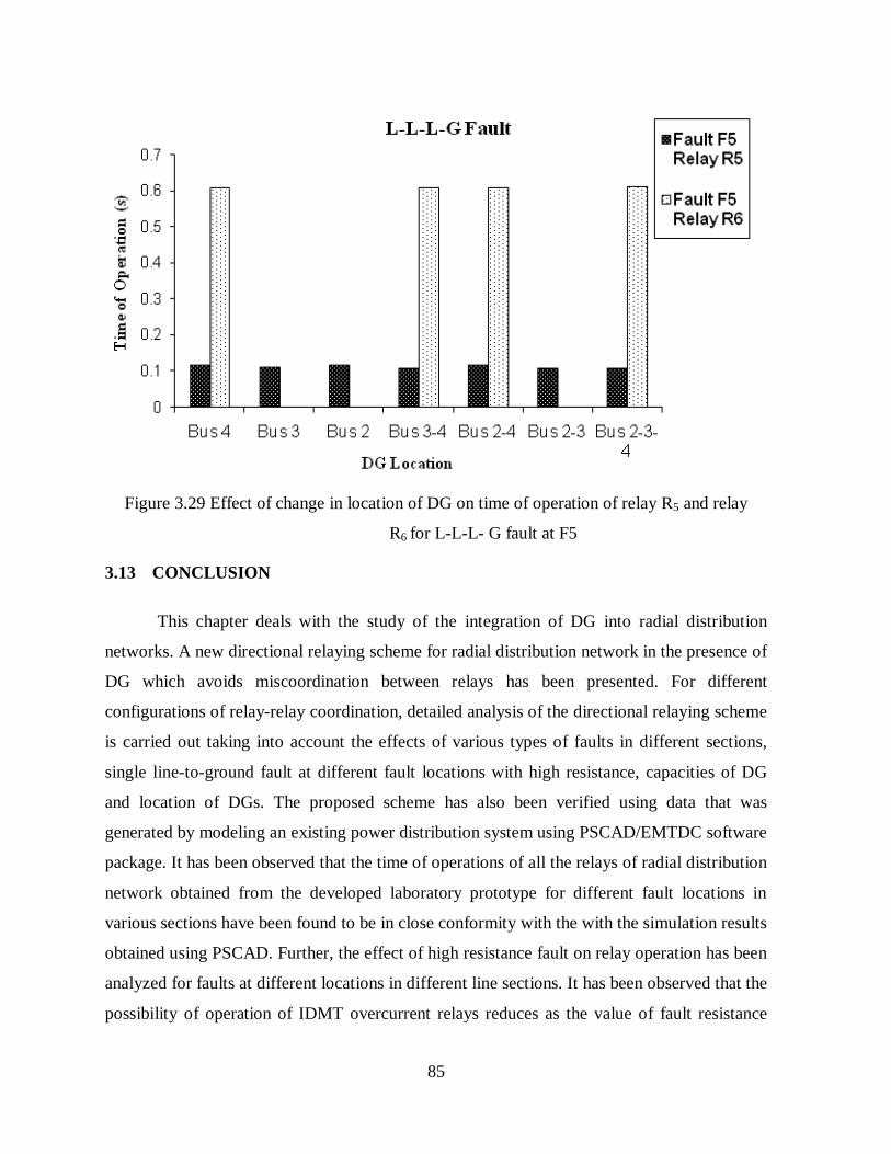
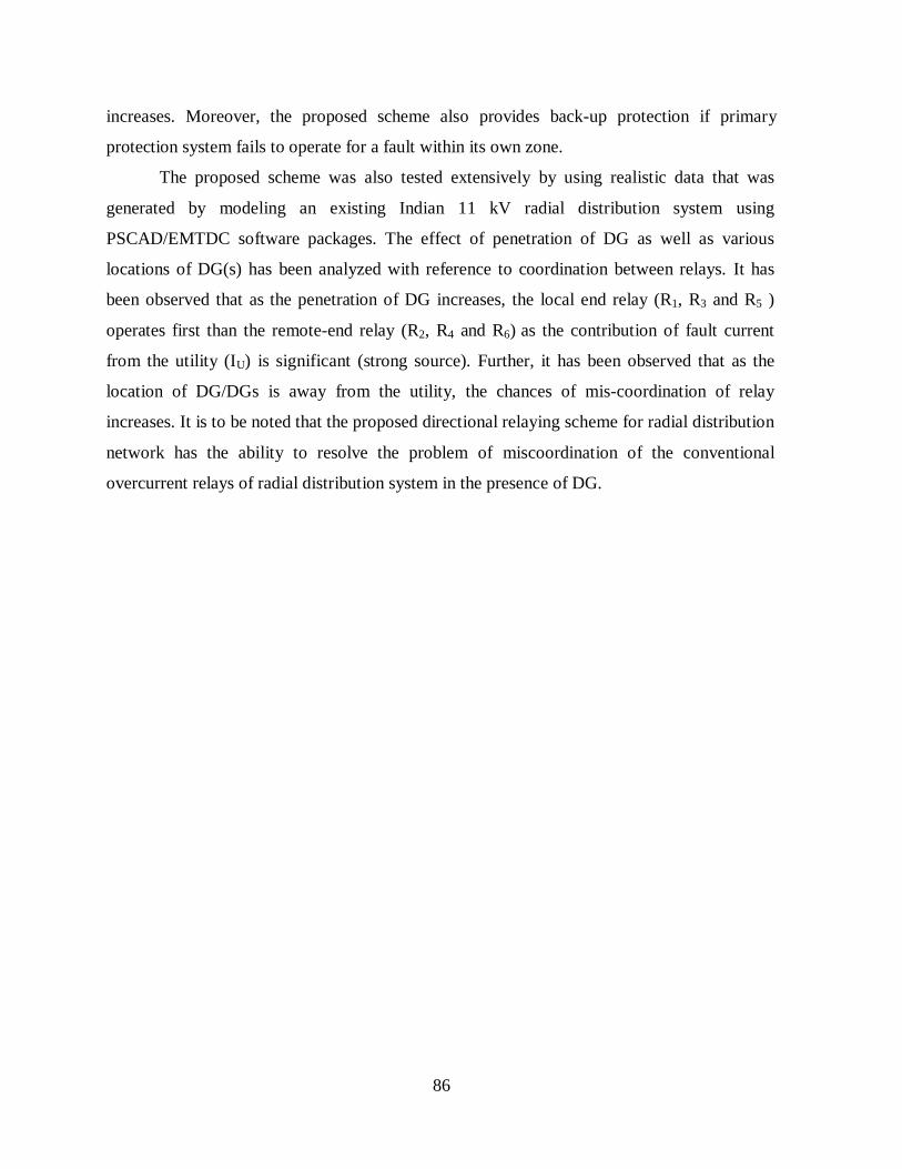
Figure 3.28 and Figure 3.29 show the simulation results in the form of time of
operation of relay R5 and relay R6 for L-G fault (minimum fault current) and L-L-L-G fault
(maximum fault current) at location F5, respectively, considering all three different
combinations of DGs as mentioned above.
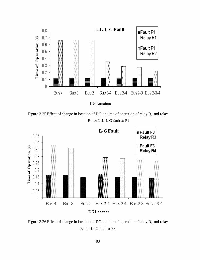
It has been observed from Figure 3.24 to Figure 3.29 that, as location of DG/DGs is
away from the utility, the chances of mis-coordination of relay increases. However, in the
proposed scheme, though the time of operation of relays (R2, R4 and R6) which operates due
to current fed by DG/DGs is higher, proper coordination between relays have been maintained
for L-G and L-L-L-G faults. The proposed scheme gives satisfactory result in the said
condition.
Figure 3.24 Effect of change in location of DG on time of operation of relay R1 and relay R2
for L- G fault at F1
83
Figure 3.25 Effect of change in location of DG on time of operation of relay R1 and relay
R2 for L-L-L-G fault at F1
Figure 3.26 Effect of change in location of DG on time of operation of relay R3 and relay
R4 for L- G fault at F3
84
Figure 3.27 Effect of change in location of DG on time of operation of relay R3 and relay
R4 for L-L-L- G fault at F3
Figure 3.28 Effect of change in location of DG on time of operation of relay R5 and relay R6
for L- G fault at F5
85
Figure 3.29 Effect of change in location of DG on time of operation of relay R5 and relay
R6 for L-L-L- G fault at F5
3.13 CONCLUSION
This chapter deals with the study of the integration of DG into radial distribution
networks. A new directional relaying scheme for radial distribution network in the presence of
DG which avoids miscoordination between relays has been presented. For different
configurations of relay-relay coordination, detailed analysis of the directional relaying scheme
is carried out taking into account the effects of various types of faults in different sections,
single line-to-ground fault at different fault locations with high resistance, capacities of DG
and location of DGs. The proposed scheme has also been verified using data that was
generated by modeling an existing power distribution system using PSCAD/EMTDC software
package. It has been observed that the time of operations of all the relays of radial distribution
network obtained from the developed laboratory prototype for different fault locations in
various sections have been found to be in close conformity with the with the simulation results
obtained using PSCAD. Further, the effect of high resistance fault on relay operation has been
analyzed for faults at different locations in different line sections. It has been observed that the
possibility of operation of IDMT overcurrent relays reduces as the value of fault resistance
86
increases. Moreover, the proposed scheme also provides back-up protection if primary
protection system fails to operate for a fault within its own zone.
The proposed scheme was also tested extensively by using realistic data that was
generated by modeling an existing Indian 11 kV radial distribution system using
PSCAD/EMTDC software packages. The effect of penetration of DG as well as various
locations of DG(s) has been analyzed with reference to coordination between relays. It has
been observed that as the penetration of DG increases, the local end relay (R1, R3 and R5 )
operates first than the remote-end relay (R2, R4 and R6) as the contribution of fault current
from the utility (IU) is significant (strong source). Further, it has been observed that as the
location of DG/DGs is away from the utility, the chances of mis-coordination of relay
increases. It is to be noted that the proposed directional relaying scheme for radial distribution
network has the ability to resolve the problem of miscoordination of the conventional
overcurrent relays of radial distribution system in the presence of DG.