Chapter 3 Process Planning and Manufacturing Planning

3.1. Introduction- Process planning deals with setting up machines while manufacturing planning refers to

setting up the production. In this chapter we will study both.- This chapter is a combination of Chapter 5 (process planning) and Chapter 10

(manufacturing planning) in the textbook and some supplementary materials from the references

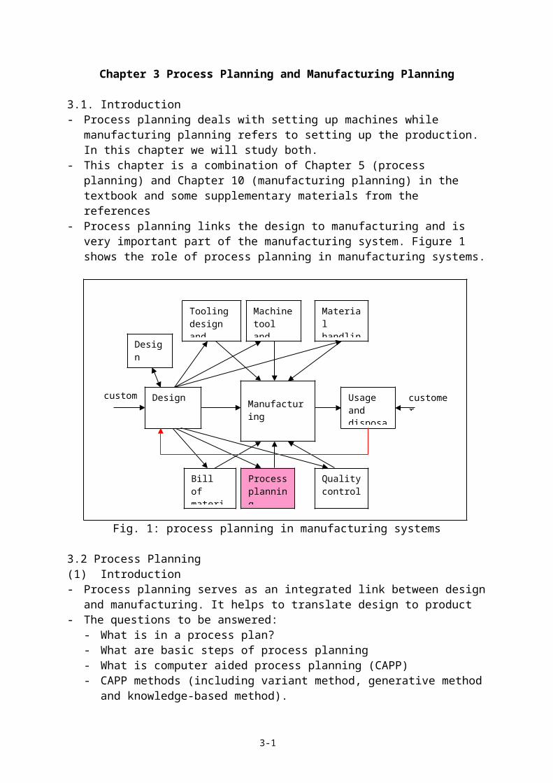
- Process planning links the design to manufacturing and is very important part of the manufacturing system. Figure 1 shows the role of process planning in manufacturing systems.

Fig. 1: process planning in manufacturing systems

3.2 Process Planning(1) Introduction- Process planning serves as an integrated link between design and manufacturing. It helps

to translate design to product- The questions to be answered:

- What is in a process plan?- What are basic steps of process planning- What is computer aided process planning (CAPP)- CAPP methods (including variant method, generative method and knowledge-based

method).- All manufacturing processes require process plans. However, we will focus on machining

process only(2) The basics of machining processes- As discussed in Chapter 2, there are many different machining processes. For example

- Turning as illustrated in Figure 2- Milling as illustrated in Figure 3- Grinding as illustrated in Figure 4

3-1

customer customer

Design analysis

Process planning

Bill of materials

Material handling

Tooling design and analysis

Machine tool and control

Quality control

Manufacturing Usage and disposal

Design

- Let us study turning (external) in a little more details- The turning process is illustrated in Figure 5

Fig. 5:

illustration of turning (external) process

- The important parameters include:- Depth of cut, d (mm or inch)- Rotation speed, N or RPM (rotation per minute)- Feed, f (mm / rev. or inch / rev.), or feed rate, fr (mm / s or inch / s)- The length of cut, L (mm or inch)

- Turning is called single point cutting as there is only one point (the cutting edge) engaged in the cut in any given time

- Some basic calculations in turning- Cutting speed, V (mm / m or inch / m):

V = DN- Machining time (minute):

where, La is the allowance distance (mm or inch)- Material removal rate, MRR, (mm3 / min, or inch3 / min):

MRR = DNfd- Tool life (Taylor’s formula), T (min):

VTn = Cwhere, n is a tool material dependent constants, C is the cutting speed at which the tool life is one minute. In particular, for HSS tools, n 0.1, for carbide tools, n 0.2, and for ceramic tools, n 0.4. The constant C is dependent on the work material and its value can be found from manufacturing handbooks. In particular, for low carbon steels, C 500.

- the cutting force, F, F = FsA

where, Fs is the specific energy and A = df is the area of cutting. The specific cutting force is a function of many factors such as work material, tool geometry, …. For low carbon steels, Fs 58.15 MPa.

- You can always check your calculation using the unit.- An example:

- given - D = 100 mm- d = 0.2 mm

3-2

N (RPM)

f (mm / rev.)

L (mm)

d (mm)

D (mm)

La

A (mm2)

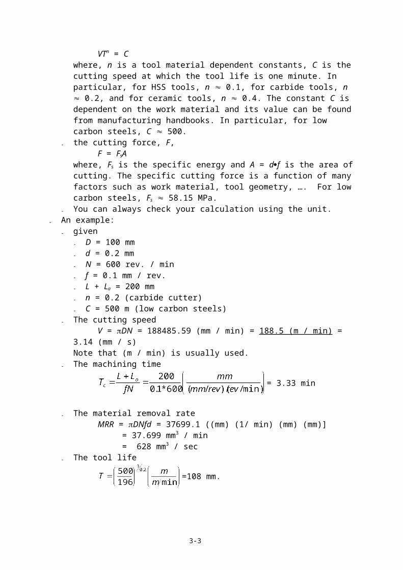
- N = 600 rev. / min- f = 0.1 mm / rev.- L + La = 200 mm- n = 0.2 (carbide cutter)- C = 500 m (low carbon steels)

- The cutting speedV = DN = 188485.59 (mm / min) = 188.5 (m / min) = 3.14 (mm / s)

Note that (m / min) is usually used.- The machining time

= 3.33 min

- The material removal rateMRR = DNfd = 37699.1 ((mm) (1/ min) (mm) (mm)]

= 37.699 mm3 / min= 628 mm3 / sec

- The tool life

=108 mm.

Note that increase the cutting speed will increase the productivity but reduce the tool life. Hence, there is an “optimal” cutting speed as shown in Figure 6.

Fig. 6: illustration of the optimal cutting speed

- The cutting force:F = FsA = 58.15*2*0.1 (MPa*mm*mm) = 11.629*10*10 (N) = 1162.9 N

(3) Determining the cutting condition- There are many models available. However, we will discuss the minimum unit cost model

only.- Reflecting a machining operation, the unit cost, Cu, is:

Cu = non-production cost per unit (loading, unloading, setup, …)+ machining cost per unit (machining time x constant)+ tool change cost per unit+ tooling cost per unit

- Thus, the minimum unit cost model:

3-3

where, C0 – machining cost with overhead ($ / min)t1 – non-production time (min)tc – machining time (min)tc – tool change time (min)(tc / T) – percentage of tool life used per unitCt – tool cost (per edge) ($)

- Note that- the machining time is:

- the tool life is:

- Substitute the machining time and the tool life equation to the above equation, it follows that:

- The solution of this model can be found by partial differentiating the equation, equating to zero and solving; and the result is as follows (fortunately, somebody has solved it for us):

and the resulting machining time is:

- The other commonly used model is production rate model, which will be discussed in the tutorial together with the manufacturing lead time

(4) An example- Given the following data:

- The parts: 50 units, L = 300 mm, D = 60 mm, f = 0.2 mm / rev., d = 1 mm- The tool: tool life coefficient: n = 0.2, C = 200- Machining cost: machining labor cost $10 / hr, overhead = 50%- Tooling cost: tool cost $30.96, 6 edges- Tool change time td = 0.5 min

- Calculation:- The machining cost: C0 = (10 + 0.5*10) = $15 hr. / 60 = $0.25 / min- The tooling cost per edge: Ct = 30.96 / 6 = $5.16- The optimal machining time:

= 84.56

- The optimal cutting speed:= 82.337 m / min

3-4

(5) Discussions:- How to deal with the constraints on speed (i.e., v vmax)?- What is the optimal feed (together with the speed)?- How to deal with the uncertainty on the cost factors (e.g., C0) and / or time factors (e.g.,

td)?- To solve these problems, we have to use linear programming (and nonlinear

programming) method(6) The procedure for machining processes planning- Step 1: analysis of part requirement (size, tolerance, surface finish, …)- Step 2: selection of raw material

- there are over 2,000 different materials available- we have learnt how to design part for better material utilization in Chapter 2

- Step 3: selection of machining sequence - Step 4: selection machine tool (we have learnt that in Chapter 2)- Step 5: selection of cutters (there are over 10,000 different cutters available)- Step 6: selection or design of fixtures and inspection equipment (optional)- Step 7: determining cutting conditions

- this includes V and f (and d for multiple passes machining)- we will focus on how to determine the cutting condition

(7) An example: Designing a machining plan for the order given below:- the work order (lot size): 200 pieces- the work design

Fig. 7: illustration of

the work design

- the work material: mild steel- the time and cost factors:

- machining cost with overhead (C0 in the optimization model): $60 / h = $1 / min- tool cost per edge (Ct in the optimization model): $60 / cutter = $10 / edge- loading and unloading time (t1 in the optimization model): 1 min / piece- tool change time (td in the optimization model): 3 min

Solution:Step 1: Analysis of part requirement (size, tolerance, surface finish, …)- the internal hole requires extra tight manufacturing tolerance and surface finish

Step 2: Selection of raw material: - material is given (given mild steel, C = 500 in the Taylor’s tool life equation)

3-5

Ra = 20 m

1000.05

Ra = 10 m

15.50.01

150 mm

- since the work design is simple, we can just order a batch of steel bars with 102 mm diameter

Step 3: Selection of machining sequence: the machining sequence:- Facing- External turning- Drilling- Boring (because of the tight manufacturing tolerance and surface finish)- Parting

Step 4: Selection machine tool- It is noted that the manufacturing tolerance and surface finish is not very high and the lot

size is low- However, several different tools are needed to complete the work- Hence, we can use a turret lathe

Step 5: Selection of cutters - use carbide tools for all operations, which is the most popular choice- n = 0.2 in the Taylor’s tool life equation

Step 6: selection of fixtures and inspection equipment (optional)- use standard hydraulic clamp of the lathe

Step 7: Determining cutting conditions and calculating the machining time and cost(a) facing- it is noted that the cutting speed changes from a maximum value, Vmax, to zero. Hence,

there is no “optimal” cutting speed. Based on experience, we choose:- N = 800 rpm- f = 0.1 mm (in radian direction)- d = 0.5 mm (in axial direction), to ensure the surface is machined

- At this time, we have:- Cutting speed:

Vmax = DN = (3.14)(102)(800) = 256224 mm / min = 256.224 m / min.- Machining time:

= (100 + 10) / (2)(0.1)(800) = 0.69 min. (Da is the clearness)

- Tool life

= [(500)(2) / (256.224)]5 = 902 min = 15 hours

- Unit cost (with the setup cost)

Cfacing =

= (1)(1) + (1)(0.69) + (1)(3)(0.69 / 902) + (10)(0.69 / 902) = $1.70(b) external turning- the depth of cut is:

d = 2 mm (the raw material diameter – the required diameter)- the feed:

f = 0.2 mm (to ensure the surface finish of Ra = 20 m)- the optimal cutting speed (note that it is independent of d and f):

3-6

= 226.9 m / min

- the machining time:

tc = = (3.14)(150+10)(100) / (1000)(0.2)(226.9) = 0.35 min

- the (optimal) tool life:

= (4)(13) = 52 min

- the unit cost (no setup cost is necessary):

Cturning =

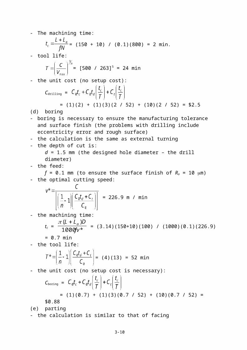
= (1)(0.35) + (1)(3)(0.35 / 52) + (10)(0.35 / 52) = $0.44(c) drilling- this can be done in a turret lathe by rotating the work- the depth (width) of cut:

d = 14 mm (to get a clearness for boring)- the cutting speed:

- the cutting speed varies from Vmax to 0 (at the center of the drill),- we choose N = 600 rmp (drilling is a severe machining operation involving large

material removal)- Hence,

Vmax = dN = (3.14)(14)(600) = 26389.78 mm / min = 263 m / min- The machining time:

= (150 + 10) / (0.1)(800) = 2 min.

- tool life:

= [500 / 263]5 = 24 min

- the unit cost (no setup cost):

Cdrilling =

= (1)(2) + (1)(3)(2 / 52) + (10)(2 / 52) = $2.5(d) boring- boring is necessary to ensure the manufacturing tolerance and surface finish (the

problems with drilling include eccentricity error and rough surface)- the calculation is the same as external turning- the depth of cut is:

d = 1.5 mm (the designed hole diameter – the drill diameter)- the feed:

f = 0.1 mm (to ensure the surface finish of Ra = 10 m)- the optimal cutting speed:

= 226.9 m / min

3-7

- the machining time:

tc = = (3.14)(150+10)(100) / (1000)(0.1)(226.9) = 0.7 min

- the tool life:

= (4)(13) = 52 min

- the unit cost (no setup cost is necessary):

Cboring =

= (1)(0.7) + (1)(3)(0.7 / 52) + (10)(0.7 / 52) = $0.88(e) parting- the calculation is similar to that of facing

- N = 800 rpm- f = 0.1 mm (in radian direction)- d = 1.5 mm (in axial direction), which is also the width of the cutter

- At this time, we have:- Cutting speed:

Vmax = DN = (3.14)(102)(800) = 256224 mm / min = 256.224 m / min.- Machining time:

= (100 – 15.5 + 10) / (2)(0.1)(800) = 0.62 min. (a hole is there)

- Tool life

= [(500)(2) / (256.224)]5 = 902 min = 15 hours

- Unit cost (no setup cost)

Cparting =

= (1)(0.62) + (1)(3)(0.62 / 902) + (10)(0.62 / 902) = $0.63(f) Total manufacturing time and cost- Total manufacturing time

tmfg = 200(tsetup + tfacing + tturning + tdrilling + tboring + tparting) = 1072 min = 17.8 hours.

Note that - the tool change may not be necessary for some operations such a small batch (a

controversy)- we can calculate the machining time each individual tool and hence, predict the

number of tool changes- Total machining cost

Cmfg = 200(Cfacing + Cturning + Cdrilling + Cboring + Cparting) = (200)($6.15) = $1230

Note that - The setup cost is included in facing- The cost can be used to calculate the profit.

3.3 Computer Aided Process Planning (CAPP)(1) Computer Aided Design changes the world of design. Can we use computer to conduct

process planning? The result is Computer Aided Process Planning (CAPP)

3-8

(2) There are three types of approaches of CAPP- variant approach- generative approach- knowledge-based approachIn fact, they all have some sort of intelligence (knowledge) involved because process planning is a creative work.

- Many CAPP systems have been developed and most of them use a combination of variant approach and generative approach. Also, most of them are still in the stage of research and development.

(3) The variant approach- The basic idea: deliver the process plan based on a master plan- The technology used: Group Technology (GT), which will be discussed in Chapter 6 in

more details.- The procedure of the variant approach:

- Define a code scheme- Group the parts into various group families- Develop a standard process plan (master plan) for each group family- Retrieve and modify the standard plan for the particular part

(4) Generative method- The basic idea: deliver the process plan based on decision logic, formulas, and rules from

data and information available.- The procedure:

- generate a representation of the part to be recognized- determine the part features based on the representation- design the process plan by matching features

- An example: generate a process plan for turning a cylinder. - Step 1: generate a part representation: a cylinder can be characterized by:

- Diameter, D- Length, L- Surface finish, Ra

- Tolerance, Tl

- Lot size (number of parts to be made), LS

Hence, the part representation is {D, L, Ra, Tl, LS}- Step 2: find the part feature, for example:

- D = 25 mm- L = 200 mm- Ra = 20 m- Tl = 0.003 mm- LS = 200

- Step 3: design the process plan based on the features. Some of the rules for selection of machine tools for turning operations are shown below:

Conditions Rule 1 Rule 2 Rule 3 Rule 4Lot size 10 XLot size 50 X XLot size 4000 XRelatively large diameterRelatively small diameter X X X XSurface finish in 40~60 m X

3-9

Surface finish in 16~32 m X X XSurface finish in 8~16 m 0.003 tolerance 0.005

X X

0.001 tolerance 0.003tolerance 0.001 X XEngine lathe X 1Turret lathe XAutomatic screw machine XCenterless grinding machine 2

where, x implies chosen, 2 means preferred, and 1 means less preferred.- Following these rules, for the above job, by using Rule 3, the selected machine tool

will be turret lathe.- For complicated parts, we need an additional step: feature recognition.(5) Feature recognition- Process planning links the design to manufacturing. However, while the links are obvious

to human operators, it may not be clear to computer. For example, we can easily recognize a hole (so a drilling operation is needed). To computers, it is just several numbers (the center, the diameter and the length). Hence, we need to a method for computer to recognize the features.

- In general, a part has two types of features:- Design features, which include geometric features (such as slot, step, hole, …),

dimensions, and tolerance- Manufacturing feature (machining feature), which are the volume to be removed, the

methods to remove them and etc.- In order to links the design features to the manufacturing features, and accordingly, to

deliver the process plan, we need first to recognize the design features from the CAD design. This is called feature recognition.

- Various feature recognition methods have been developed. Here, we will only study the Attributed Adjacency Graph method

(6) Feature recognition using Attributed Adjacency Graph (AAG)- The AAG method is applicable to prismatic parts only.- The basics of a AAG: an AAG is a graph G = (N, A, T), where, N is the set of nodes, A is

the set of arcs, and T is the set of attributes to arcs in A such that- For every face (surface) f in F, there exists a unique node n in N- For every edge e in E, there exists a unique arc a in A, connecting nodes ni and nj,

corresponding for face fi and face fj, which share the common the common edge e- Every arc a in A is assigned an attribute t, where

- t = 0 if the faces sharing a concave angle (or inside edge)- t =1 if the faces sharing a convex angle (or outside edge)this is shown in Figure 7.

3-10

Fig. 7: illustration of face connections in AAG

- Note that each primary feature has a distinct AAG as shown in Figure 8- The procedure of feature recognition using AAG:

- Step 1: generate the AAG of the part- Step 2: generate the corresponding matrix (so computer can manipulate it)- Step 3: simplify the matrix- Step 4: find the simplified AAG- Step 5: match features in the AAG to determine the part feature.

- An example:- The example is shown in Figure 9: it can be seen that the part consists of two features:

a slot and a blind pocket.- Mark the surfaces- Generate the AAG- Generate the corresponding matrix (the textbook has a typo). Note that if two faces

are not connected, then a “9” is assigned in the matrix for easy of manipulation. The resulting matrix is shown below:

3-11

F1

F2

F1

F2

0

F1F2

F1

F2

1

- Simplify the matrix: deleting all the columns and rows which consist of only 1s and 9s. In the above matrix, it includes columns: 6, 7, 8, 9, 10, 14, 15 and rows: 6, 7, 8, 9, 10, 14, 15. The resulting matrix is as follows:

- Find the simplified AAG (Figure 9)- By comparing to Figure 8, it is seen that the part consists of two features: a slot and a

blind pocket.- Based on the recognized feature, we can then design the process plan. For example, the

blind pocket feature is defined by:- Length: 2.5 0.01- Width: 1.4 0.01- Depth: 0.75 0.01- Corner radius: 025- Side wall thickness- Bottom wall thickness- Side surface finish- Bottom surface finish- Axial clearance- Radial clearance- Connecting face- Bottom face- Side faces- Fillet facesThe matching pocket machining rule is:- machining operation: end milling- machining sequence: roughing and then finishing- tool selection- machining condition- inspection (check point)- …

3-12

- The AAG method can also deal with rotational parts. However, it cannot deal with sculpture surfaces (used in molds and dies).

3.4 Manufacturing Planning(1) Manufacturing planning, also called production planning (in Europe), is a step up from

the process planning as illustrated in Figure 10.

Fig. 10: Illustration of process planning and manufacturing planning

(2) In the previous sections, we have studied how to develop a process plan. In this section, we will discuss how to develop a manufacturing planning.

(3) As shown in Figure 11, the major elements of an integrated production planning include:(a) demand management(b) aggregate planning(c) master production schedule(d) material requirement planning(e) capacity planning(f) order release

(4) Note that:- Demand management is to forecast the customer demands. We have discussed the

forecasting method in a separate course and hence, will not be discussed. Here.- Aggregate production planning (b) is to determine an overall production plan- Master production schedule (c) is to determine the production schedule for each

individual product- Material requirement planning (d) is to determine when to purchase parts and sub-

assembly- Capacity planning is to plan the future development. Again, we will not discussed that.- Order release is a document that describes the manufacturing plan. It is a collection of all

decision made the planning stage.- In the following sections, we will focus on (b), (c), and (d).

3-13

processes

Manufacturing plan

Fig. 11: illustration of manufacturing planning

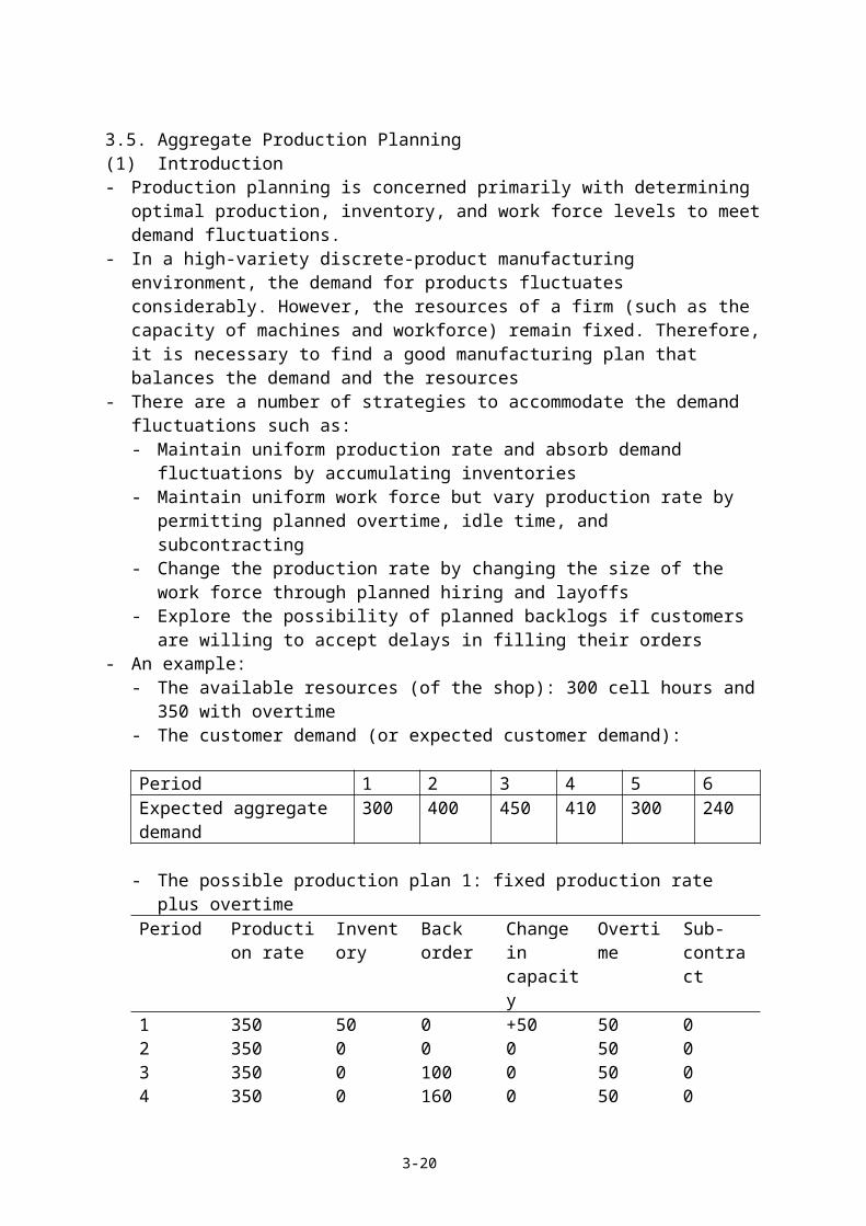
3.5. Aggregate Production Planning(1) Introduction- Production planning is concerned primarily with determining optimal production,

inventory, and work force levels to meet demand fluctuations.- In a high-variety discrete-product manufacturing environment, the demand for products

fluctuates considerably. However, the resources of a firm (such as the capacity of machines and workforce) remain fixed. Therefore, it is necessary to find a good manufacturing plan that balances the demand and the resources

- There are a number of strategies to accommodate the demand fluctuations such as:- Maintain uniform production rate and absorb demand fluctuations by accumulating

inventories- Maintain uniform work force but vary production rate by permitting planned

overtime, idle time, and subcontracting- Change the production rate by changing the size of the work force through planned

hiring and layoffs- Explore the possibility of planned backlogs if customers are willing to accept delays

in filling their orders- An example:

- The available resources (of the shop): 300 cell hours and 350 with overtime - The customer demand (or expected customer demand):

3-14

Shop floor

Customer orders

Demand management

Aggregate planning

Master production schedule

Capacity planning

Material requirement planning

Order release

Design

Bill of materials

Purchasing

Vendors

Period 1 2 3 4 5 6Expected aggregate demand 300 400 450 410 300 240

- The possible production plan 1: fixed production rate plus overtimePeriod Production

rateInventory Back

orderChange in capacity

Overtime Sub-contract

1 350 50 0 +50 50 02 350 0 0 0 50 03 350 0 100 0 50 04 350 0 160 0 50 05 350 0 110 0 50 06 350 0 0 0 50 0

Note that the calculations above are simple. For example, in the first column, using the full capacity of the shop (350) while the required production rate (300), the inventory is 350 – 300 = 50, the back order is 0, the capacity is also 50 representing a left over production rate of 50. The overtime is 50 and there is no need for subcontract. Also, it should be noted that the shop runs at its maximum capacity because of the expected higher customer demand in later time periods.- The possible production plan 2: variable production rate with overtime and

subcontract.Period Production

rateInventory Back

orderChange in capacity

Overtime Sub-contract

1 400 100 0 +100 60 402 400 100 0 0 60 403 400 50 0 0 60 404 400 40 0 0 60 405 250 0 10 -50 0 06 250 0 0 0 0 0

- Questions:- Which plan is better?- Is there any better plan?

- The Answer: mathematical programming

(2) The mathematical programming problems can be represented as follows: - Find x such that:

min f(x) (or max f(x))s. t.: g(x)

- There are various types of mathematical programming including- unconstrained programming (we have seen that in the machining process optimization

example)- constrained programming- linear programming (the objective function and the constrains are all linear)- nonlinear programming- integrate programming- dynamic programming- ……

- There are also many methods for solving the problems, such as

3-15

- Simplex method- Hill climbing method- Newton – Raphson method- ……

(3) Let us consider a simple example of unconstrained programming- the problem is to find x (single variable) such that

min f(x)- this can be done by partial differentiating and equating zero and solving:

(x* denotes the optimal solution)

- an example:f(x) = 2x2 – x + 1

this is illustrated below:

Fig. 12: Illustration of minimization

Note that this is the minimum solution and there is no maximum solution.- more complicated problems may include:

- has no analytical solution

- multiple variables x = (x1, x2, …, xn)- constrains (note that in the above example, given the constrain there will be a

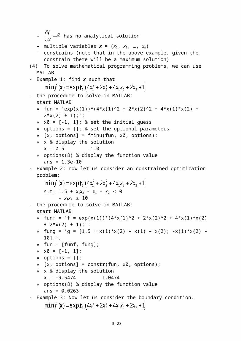
maximum solution)(4) To solve mathematical programming problems, we can use MATLAB.- Example 1: find x such that

- the procedure to solve in MATLAB:start MATLAB» fun = ‘exp(x(1))*(4*x(1)^2 + 2*x(2)^2 + 4*x(1)*x(2) + 2*x(2) + 1);’;» x0 = [-1, 1]; % set the initial guess» options = []; % set the optional parameters» [x, options] = fminu(fun, x0, options);

3-16

f(x)

xx* = 1/4

constrains

Maximum solution under constrain

» x % display the solutionx = 0.5 -1.0

» options(8) % display the function valueans = 1.3e-10

- Example 2: now let us consider an constrained optimization problem:

s.t. 1.5 + x1x2 – x1 – x2 0- x1x2 10

- the procedure to solve in MATLAB:start MATLAB» funf = ‘f = exp(x(1))*(4*x(1)^2 + 2*x(2)^2 + 4*x(1)*x(2) + 2*x(2) + 1);’;» fung = ‘g = [1.5 + x(1)*x(2) – x(1) – x(2); -x(1)*x(2) – 10];’;» fun = [funf, fung];» x0 = [-1, 1]; » options = []; » [x, options] = constr(fun, x0, options);» x % display the solution

x = -9.5474 1.0474» options(8) % display the function value

ans = 0.0263- Example 3: Now let us consider the boundary condition.

s.t. 1.5 + x1x2 – x1 – x2 0- x1x2 10x1 0x2 0

- the procedure to solve in MATLAB:start MATLAB» funf = ‘f = exp(x(1))*(4*x(1)^2 + 2*x(2)^2 + 4*x(1)*x(2) + 2*x(2) + 1);’;» fung = ‘g = [1.5 + x(1)*x(2) – x(1) – x(2); -x(1)*x(2) – 10];’;» fun = [funf, fung];» x0 = [-1, 1]; » options = [];» vlb = zero(1, 2); % set the lower boundary x(1) > 0 and x(2) > 0» vub = []; % there is no upper boundary on x(1) and x(2)» [x, options] = constr(fun, x0, options, vlb, vub);» x % display the solution

x = 0 1.5» options(8) % display the function value

ans = 8.5- You can get more information directly when runing MATLAB by using help commands

and / or demos

(5) The mathematical programming model for Aggregate Production Planning- Several models have been developed. We will study just one:- The model

Minimize total system costSubject to: inventory balance between the demand and production

labor balance

3-17

overtime, under-time time, work force and production constraints- Mathematically, this is:

minimize Z = cxXt + cwWt + coOt + cuUt + ciIt+ + csIt

- + chHt + cfFt

subject to: , for t = 1, 2, …, TWt = Wt-1 + Ht – Ft

Ot – Ut = kXt – Wt

Xt, Wt, Ot, Ut, It+, It

-, Ht, Ft 0

where, Z = total production system cost dt = aggregate demand in period tXt = production units scheduled in period tcx = cost of production excluding labor per hourWt = regular work force level in period tcw = cost of regular labor per hourOt = overtime work force level in period tco = cost of overtime labor per hourUt = under-time work force level in period tcu = cost of under-time labor per hour (waste)Ht = new labor force added in hours in period tch = cost of hiring regular time abor per hourFt = layoffs in hours in period tcf = cost of layoffs per hourIt

+ = inventory in stock at the end of period tci = cost of unit inventory holding per hourIt

- = shortages at the end of period tcs = cost of a shortage per hourk = labor hours required to produce a unit T = number of periods in the planning horizon

- Note- The model has many variables to be determine (8 variables per time period)- It is a linear programming model and can be solved using MATLAB.

(6) An example- Following the example above, we assume T = 2 (this is for simplicity and in fact, T = 6 is

given) the cost factors are:cx = $100 / h, cw = $14 / h, co = $20 / h, cu = $50 / h, ch = $14 / hcf = $30 / h, ci = $3 / unit / h, cx = $400 / h, k = 1 (one hour per unit)

Also, for the purpose of calculation, let:x(1) = X1, x(2) = X2, x(3) = W1, x(4) = W2, x(5) = O1, x(6) = O2, x(7) = U1, x(8) = U2,x(9) = I1

+, x(10) = I2+, x(11) = I1

-, x(12) = I2-, x(13) = H1, x(14) = H2, x(15) = F1,

x(16) = F2,- The procedure

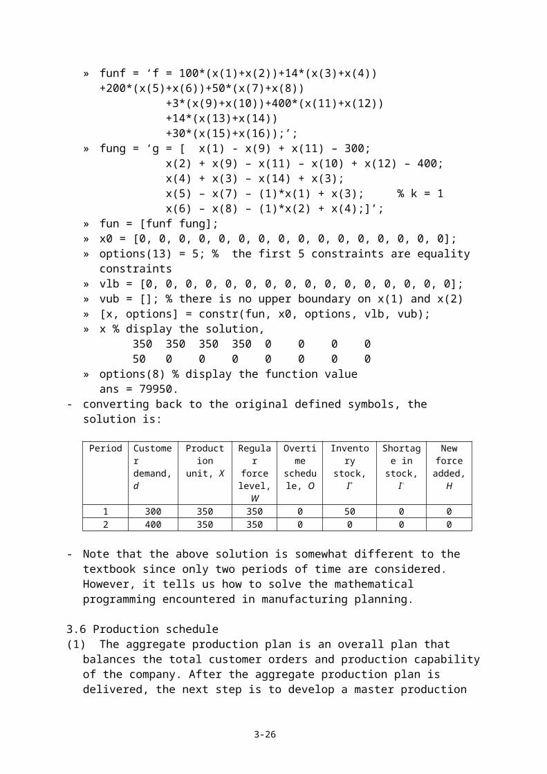
start MATLAB» funf = ‘f = 100*(x(1)+x(2))+14*(x(3)+x(4))+200*(x(5)+x(6))+50*(x(7)+x(8))

+3*(x(9)+x(10))+400*(x(11)+x(12))+14*(x(13)+x(14))+30*(x(15)+x(16));’;

» fung = ‘g = [ x(1) - x(9) + x(11) – 300;x(2) + x(9) – x(11) – x(10) + x(12) – 400;x(4) + x(3) – x(14) + x(3);

3-18

x(5) – x(7) – (1)*x(1) + x(3); % k = 1x(6) – x(8) – (1)*x(2) + x(4);]’;

» fun = [funf fung];» x0 = [0, 0, 0, 0, 0, 0, 0, 0, 0, 0, 0, 0, 0, 0, 0, 0]; » options(13) = 5; % the first 5 constraints are equality constraints» vlb = [0, 0, 0, 0, 0, 0, 0, 0, 0, 0, 0, 0, 0, 0, 0, 0];» vub = []; % there is no upper boundary on x(1) and x(2)» [x, options] = constr(fun, x0, options, vlb, vub);» x % display the solution,

350 350 350 350 0 0 0 050 0 0 0 0 0 0 0

» options(8) % display the function valueans = 79950.

- converting back to the original defined symbols, the solution is:

Period Customer demand, d

Production unit, X

Regular force

level, W

Overtime schedule,

O

Inventory stock, I+

Shortage in stock, I-

New force

added, H1 300 350 350 0 50 0 0 2 400 350 350 0 0 0 0

- Note that the above solution is somewhat different to the textbook since only two periods of time are considered. However, it tells us how to solve the mathematical programming encountered in manufacturing planning.

3.6 Production schedule(1) The aggregate production plan is an overall plan that balances the total customer orders

and production capability of the company. After the aggregate production plan is delivered, the next step is to develop a master production schedule, which specify when each and every product shall be made.

- There are two correlated terms: master production schedule and production operations schedule.

- Master production schedule deals with the overall time schedule problems of the production such as whether an overtime is necessary. It is usually easier to conduct.

- Operations schedule deals with- Machine loading – how to assign the jobs to the work centers (workstations) and

when- Job sequencing – which job shall be done first and when

- We will focus on operations schedule.- The objectives of operations schedule may be

- Meet the due dates- Minimize manufacturing throughput time- Minimize work-in-process- Maximize work center utilization

- There are two important indices in operations scheduling:- Loading time = setup time + Q * unit run time (processing time)- Manufacturing throughput time = setup time + Q * unit run time + move and queue

time, where, Q is the lot size (processing time + waiting time).

(2) The basic rules of operations schedule include:

3-19

(a) First-come, first-served (FCFS): assign jobs on a first-come, first-served basis. This rule is “blind” with respect to all other factors such as due date and urgency.

(b) Shortest processing time (SPT): give the highest priority to the jobs with the shortest processing time (so it can get a higher cash flow). This rule results in the lowest mean completion time and hence, the lowest work-in-process inventory.

(c) Earliest due date (EDD): give the highest priority to the jobs with the earliest due date.(d) Least slack (LS): assign the highest priority to the job with least slack. The slack is

defined as follows:Slack = time remaining until due date – process time remaining

(e) Least slack per operation (LSPO): assign priority based on the smallest value obtained by dividing the slack by the number of remaining operations

(f) Critical ratio (CR): assign priority based on a critical index defined below:

where, time remaining until due data = due date – now and lead time includes setup, run, move, and queue times.

(3) Now let us consider a simple example where multiple jobs enter a work center as shown below:

- An example: WSC Manufacturing company received four orders, A, B, C, and D sequentially on day 10, with the expected due date, the remaining process time and the number of remaining operations shown below.

Job Due date Remaining process time

Number of remaining operations

A 17 4 8B 29 18 18C 27 8 16D 26 12 2

- Using different rules, different job sequences may be obtained.- use the FCFS rule (first-come, first-serve): A, B, C, D- use the SPT rule (shortest production time): A, C, D, B- use the EDD rule (earliest due date): A, D, C, D- use the LS rule (least slack): the slack time is determined by:

slack time = time remaining until due date – process time remainingfor job A: slack = (17 – 10) – 4 = 3 daysfor job B: slack = (29 – 10) – 18 = 1 day

3-20

Work center

A

B

C

D

for job C: slack = (27 – 10) – 8 = 9 daysfor job D: slack = (26 – 10) – 12 = 4 daystherefore, the job sequence is: B, A, D, C

- use the LSPO rule (least slack per operation rule): the slack per operation is defined as:

for job A: slack = 3 / 8 = 0.375for job B: slack = 1 / 18 = 0.055for job C: slack = 9 / 16 = 0.5625for job d: slack = 4 / 2 = 2therefore, the job sequence is: B, A, C, D

- use CR rule (critical ratio), the critical ratio is defined as follows:

for job A: CR = (17 – 10) / 4 = 1.75 daysfor job B: CR = (29 – 10) / 18 = 1.05 daysfor job C: CR = (27 – 10) / 8 = 2.215 daysfor job D: CR = (26 – 10) / 12 = 1.33 daystherefore, the job sequence shall be: B, D, A, C

- from the above example, it is seen that the job sequence may be different under different rules.

(4) Scheduling using Graph Theory- In the above example, we have seen how to design a schedule for multiple jobs competing

a same work center. In this section, we will study how to design a schedule for a single job that requires several operations and hence competing different work centers as illustrated below:

- Note that- Different task may require different amount of time to process the job- The process of a task may depend on the completion of other tasks. (for example, in

order to perform a reaming operation, we must do the drilling first)- There are two methods, Gantt Chart and PERT Chart, that can help and they are both

based on graph theory

(5) Gantt chart- Gantt chart is the most widely used time management tool.- The basic idea of Gantt is just to add a dimension to the time axis: the horizontal axis is

the time while the added vertical axis is the activities (or tasks). The time spend of an activity is represented by means of a bar in the graph. The correlation among the activities are shown by the start-to-end dates.

3-21

wc1

wc2

wcn

- To describe the correlation among the activities of a project, we first develop a “start-to-end” table as the example shown below:

Activity Immediate predecessors duration (weeks)A - 5B - 3C A 8D A, B 7E - 7F C, E, D 4G F 5

- The Gantt chart is shown in the following figure. The difference between two scheduled activities is called the slack of the activities.

- From a Gantt chart, a schedule may have two ways to start:- Early start: all activities start as soon as possible, without violating the precedence

relations- Late start: all activities start as late as possible, as long as the finish date is not

compromised- In the above example, the Gantt chart uses early start. Note that the shaded boxes show

the critical path of the project, which has no slack time. Any delay along the critical path will result in the delay of the project.

- Using the same idea, one can generate the late start Gantt chart as well.- Gantt chart can accommodate additional information. These include:

- The interpretation of the activities- The work breakdown structure number (note that each activity corresponds to WBS

task).- The original scheduled milestone (denoted by )- The review date - The rescheduled milestone (denoted by )- The completed milestone (denoted by )

- An example is shown below.

No. Task/milestone WBS

3-22

A

B

C

D

E

F

G

5 10 15 20

5 10 15 20 25A 1.1B 1.2C 1.3D 1.4E 1.5F 1.6G 1.7

- There are computer software systems that will help to generate the Gantt chart.

(6) PERT chart and CPM method – the basic idea- The basic approach to all project scheduling is to form an actual or implied graph that

graphically portrays the relationship between the tasks and milestones in the project. Gantt chart is one of them and PERT/CPM chart is the other, which is more powerful.

- PERT stands for program evaluation and review technique. CPM stands for critical path method. Although they are different, nowadays, PERT/CPM are used together for scheduling.

- PERT/CPM is based on a diagram that represents the entire project as a network of arrows and nodes, resulting the AOA (Activity On Arrows) and AON (Activity on Node) methods. We will discuss both methods.

- To apply PERT/CPM, we must answer the following questions:- What are chief project activities? (the WBS)- What are sequencing requirement? (the start-to-end table)- Which activities can be conducted simultaneously?- What are the estimated requirements for each activity?

- There are a number of advantages that make PERT/CPM the prime tool for scheduling

(7) PERT/CPM method – AOA network- AOA networks, as its name indicated, are made of a number of arrows. Each arrow

represents an activity. Note:- Each arrow has two events: a head and tail- Each event represents a point in time - The head represents the beginning event of the activity- The tail represents the completing event of the activity- The direction of the arrow indicates the progress of the project (time)

- The rules for constructing an AOA are as follows:

- rule 1: each activity is represented by one and only arrow in the network

3-23

i j

Beginning state

Completing state

Project direction

- rule 2: no two activities can be identified by the same head and tail events (to do this, it may be necessary to add some dummy events)

- rule 3: to ensure the correct representation in the AOA diagram, the following questions must be answered as each activity is added to the network:(a) Which activities must be completed immediately before this activity can start?(b) Which activities must immediately follow this activity?(c) Which activities must occur concurrently with this activity?

- An example: Develop an AOA network for the same data in the previous section. - Solution:

- From the example, we know the correlation among the activities

Activity Immediate predecessors duration (weeks)A - 5B - 3C A 8D A, B 7E - 7F C, E, D 4G F 5

- First, it is good to have a common starting point. So, we start at state 1.- Second, identify all activities that have no predecessors, which are A, B, and E. They

lead to states 2, 3, 4.

- After the completion of A, B, E, we can then start C and D. C leads to state 5. However, D cannot start until the completion of both A and B. Since there is no correlation between A and B, hence a dummy state, 6, is introduced. The activities to complete this states, D1 and D2, require zero time. From state 6, we can then have D, which leads to 7.

- After the completion of C, D, and E, we can start F. At this point, it is interesting to know that there are no activities between 5 to 7 and between 4 to 7. Hence, these two states can be deleted. In addition, state 6 is a dummy state (both D1 and D2 require no time to complete). Hence, it can be merged to the state 3. The resulting diagram is shown below.

3-24

1

2

A

B

E

D

C5

3

D1

6 7D2

8F

4

- After the completion of F, G can start.- Finally, affiliate the required time to the activities, the AOA network is completed.

- Based on the AOA network, we can find much useful information for scheduling as discussed below.

- The event matrix shows the correlation among the activities

Ending event1 2 3 4 5 6

1 X X X2 X X

Starting event 3 X4 X5 X6

- The sequences of the network:Sequence number Events in the

sequenceActivities in the

sequenceSum of activity

times1 1-2-4-5-6 A, C, F, G 222 1-2-3-4-5-6 A, (D), D, F, G 213 1-3-4-5-6 B, D, F, G 194 1-4-5-6 E, F, G 16

- Observations:- Among all the sequences, the one that takes most time is the critical path (Sequence 1

in the above example). A delay in the critical path will result in a delay of the project.- Activities not on the critical path have slack time and can be delayed to start in

temporally bases. (In the above example, task C is not on the critical path, and hence can be delayed to start)

- In general, there may be two types of slacks:- Free slack represents the time that an activity can be delayed without delaying the

start of any succeeding activity and the end of the project. The activities whose

3-25

1 3

2

4 5 6

A, 5

B, 3

E, 7

C, 8

D, 7 F, 4 G, 5

end events are on the critical path have free slacks (In the above example, C has a free slack time 22 – 16 = 8).

- Total slack is the time that the completion of an activity can be delayed without delaying the end of the project. The activities whose end events are not on the critical path have total slacks. The increase of the total slack time will effect the subsequent tasks (In the above example, B has a total slack time of 22 – 19 = 3. However, different to the free slack time, if B takes this period of time, D will be affected).

- Important times in the schedule include the earliest and latest times each event can take place without causing a schedule overrun. This information is needed to calculate the critical path as well as balance the project load (work load and budget).

- Early time: - Notation: the early time of a event i is denoted as ti, - Meaning: early time is the length of the longest sequence from the start node (event 1)

to event i. (note that ti = 0 implies the corresponding activities have no precedence constraints and can begin as early as possible.

- Calculation formula: to determine ti for event i, a forward pass is made through the network. Let Lij be the duration or length of activity (i, j), then:

tj = maxi[ti + Lij] for all (i, j) activities defined.

- for instance, in the above example, the early time of event 3 is determined be:t3 = max[t1 + L13, t2 + L23] = max[0+3, 0+5] = max[3, 5] = 5.

- it is interesting to know that the last early time is the total project time. For instance, in the above example, the early time of event 6 is:

t6 = max[t5 + L56] = 17 + 5 = 22.

- Late time:- Notation: the late time of a event i is denoted as Ti, - Meaning: late time is the length of the shortest path from the end of the project to the

activity. - Calculation formula: to determine the late time, we start from the end of the project

and make a backward pass through the network to the activity:Tj = minj[Ti - Lij] for all (i, j) activities defined.

- For instance, in the above example, the late time for event 2 is:T2 = min[T3 – L23, T4 + L24] = max[6-0, 13-8] = max[6, 5] = 5.

- In the above example, time early time and the late time are summarized below:Event (i) early time (ti) late time (Ti)1 0 02 5 53 5 64 13 135 17 176 22 22

- We can also calculate the start and finish time of each activity:- ESij = ti, early start time is the earliest time activity (i, j) can start without violating

any precedence relations

3-26

- EFij = ESij – Lij, early finish time is the earliest time activity (i, j) can finish without violating any precedence relations

- LFij = Tj, late finish time is the latest time activity (i, j) can start delaying the completion of the project.

- LSij = LFij – Lij, late start time is the latest time activity (i, j) can start without delaying the completion of the project

- Furthermore, we can calculate the slack times as well:- TSij = LSij – ESij = LFij - EFij, for activity (i, j), the total slack time is the difference

between its late start and its early start times. It is also equal to the difference between its late finish time and early finish time.

- FSij = tj – (ti – Lij), assuming that all activities are started as soon as possible, for activity (i, j), the free slack time is the difference between its early time of its end event j and the sum of the early time of its start even i plus its length.

- For the example above, the following table summarizes these times:

activity (i, j) Lij ESij EFij LFij LSij TSij FSij

A 1, 2 5 0 5 5 0 0 0B 1, 3 3 0 3 6 3 3 2C 2, 4 8 5 13 13 5 0 0D 3, 4 7 5 12 13 6 1 1E 1, 4 7 0 7 13 6 6 6F 4, 5 4 13 17 17 13 0 0G 5, 6 5 17 22 22 17 0 0D1 2, 3 0 5 5 6 6 1 0

- Although computer software systems have been developed to generate PERT / CPM and calculate the important times, it is a good practice to work on calculations by hand as it will help you to gain an insight look of the project.

(8) PERT/CPM method – AON network- Similar to the AOA method but focus on the activity (each node represent a task together

with its early start time and late start time)- It can be shown that the topology of AON and AOA are the same.- For the example above, the AON network is shown below.

3-27

Start

A

B

E

C

D F G End

ES = 0LS = 0

ES = 0LS = 0

ES = 5LS = 5

ES = 0LS = 3

ES = 5LS = 6

ES = 0LS = 6

ES = 13LS = 13 ES = 17

LS = 17ES = 22LS = 22

(9) Note

- When a master production schedule is developed, it is necessary to run a computer simulation (called rough-cut capacity planning) to determine the feasibility of the plan. There are several commercial software systems available, such as WINTESS.

- The most complicated case is to deal with multiple jobs multiple tasks scheduling. Its solution can be found using the queuing theory, which is unfortunately beyond the scope of this class.

3.7 Material requirement planning(1) Introduction- After the master production schedule is delivered, Material Requirement planning (MRP)

carries out to prepare for the production- MRP is used for managing inventories of components, sub-assemblies, parts, materials

and etc. The primary objective of MRP is to determine how many these components, sub-assemblies and etc. should be manufactured or purchased and when.

(2) The key steps in MRP include:- study the product (bill of material)- determine the gross requirement- determine the net requirement- order release

(3) Study of the product- A product is usually described by its design (blue print) and a bill of material, which

shows how the product is assembled.- Following is an example from a bill of material- Note that

- The root item is the end product which is the independent demand from the customer- The other items are dependent demands which are the components or sub-assemblies

of the product

(4) Determine the gross requirement- The gross requirement can be determined from the bill of material, where, “E” implies

end product, S means lost subassembly, C means components and M means materials.

3-28

Fig. 14: Illustration of a product assembly from a bill of material

- For the example above, it is seem the gross requirements are:Demand of S1 = 1 x demand of E1 = 50 unitsDemand of S2 = 2 x demand of E1 = 100 unitsDemand of C1 = 1 x demand of S1 = 50 unitsDemand of C2 = 2 x demand of S1 = 100 unitsDemand of C3 = 2 x demand of S2 = 200 unitsDemand of C4 = 3 x demand of S2 = 300 unitsDemand of C5 = 1 x demand of S2 = 100 units

- Note that the common-use items shall be manufactured / purchased at a same time to reduce the setup cost.

(5) Determine the net requirement- Productions are often continuous and hence, there are parts in the inventory. This is called

on-hand inventory- The gross demand substrates the on-hand inventory is the net requirement (6) Lot sizing problem- When making or purchasing parts for the production, it is a usual practice to have small

on-hand inventory for the “rainy days”.- The question is when large the on-hand inventory shall be. This problem is referred to the

lot sizing problem- The lot sizing problem can be described by the following mathematical model:

Minimize

Subject to: xj + Ij-1 – Ij = dj, for j = 1, 2, …, Txj 0Ij 0

where, j = 1, 2, …, TT = number of periods in the planning horizon

3-29

E1

M1 (1) M2 (1) M3 (2) M4 (2) M5 (1)

C1 (1) C2 (2) C4 (1)C4 (3)C3 (2)

S1 (1)S2 (2)

dj = demand in period jxj = production quantity in period j (a decision variable)Ij = inventory level in period j (a decision variable)hj = holding cost per unit in period jcj = variable production cost per unit in period jSj = setup cost in period j

- This is a mathematical programming problem and there are several methods available to solve it, such as:- Wagner and Whitin algorithm (finds the optimal solution)- Naidu and Singh Algorithm (finds a feasible solution)

- We can use MATLAB to solve it.

(7) Order release- The last step in the production planning is order release. At this time, everything is set

and ready to go.- The order release represents the end of process planning. It also brings in a new phase in

manufacturing: production - The manufacturing plan will be monitored and controlled all the time during production.

Tutorial 1:The maximum production rate model and manufacturing lead-timeUse AAG to find the features of a part

Tutorial 2:Use MATLAB to solve optimization modelsUse MATLAB to solve the lot sizing problem in the textbook

Tutorial 3:Gantt Chart and PERT Chart (Reference [1])

AssignmentChapter 4: 7, 9, 15Chapter 10: 6, 11, 12

3-30