chapter 5 harmonic oscillator and coherent states · chapter 5 harmonic oscillator and coherent...
TRANSCRIPT

Chapter 5
Harmonic Oscillator and CoherentStates
5.1 Harmonic Oscillator
In this chapter we will study the features of one of the most important potentials inphysics, it’s the harmonic oscillator potential which is included now in the Hamiltonian
V (x) =mω2
2x2 . (5.1)
There are two possible ways to solve the corresponding time independent Schrodingerequation, the algebraic method, which will lead us to new important concepts, and theanalytic method, which is the straightforward solving of a differential equation.
5.1.1 Algebraic Method
We start again by using the time independent Schrodinger equation, into which we insertthe Hamiltonian containing the harmonic oscillator potential (5.1)
H ψ =
(− ~2
2m
d2
dx2+mω2
2x2
)ψ = E ψ . (5.2)
We rewrite Eq. (5.2) by defining the new operator x := mωx
H ψ =1
2m
[(~i
d
dx
)2
+ (mωx)2
]ψ =
1
2m
[p2 + x2
]ψ = E ψ . (5.3)
We will now try to express this equation as the square of some (yet unknown) operator
p2 + x2 → (x + ip)(x − ip) = p2 + x2 + i(px − xp) , (5.4)
but since x and p do not commute (remember Theorem 2.3), we only will succeed by takingthe x − p commutator into account. Eq. (5.4) suggests to factorize our Hamiltonian bydefining new operators a and a† as:
95

96 CHAPTER 5. HARMONIC OSCILLATOR AND COHERENT STATES
Definition 5.1 a := 1√2mω~(mωx + ip) annihilation operator
a† := 1√2mω~(mωx − ip) creation operator
These operators each create/annihilate a quantum of energy E = ~ω, a propertywhich gives them their respective names and which we will formalize and prove later on.For now we note that position and momentum operators are expressed by a’s and a†’slike
x =
√~
2mω
(a + a†
)p = −i
√mω~
2
(a − a†
). (5.5)
Let’s next calculate the commutator of the creation and annihilation operators. It’squite obvious that they commute with themselves
[ a , a ] =[a† , a†
]= 0 . (5.6)
To find the commutator of a with a† we first calculate aa† as well as a†a
a a† =1
2mω~[(mωx)2 + imω [ p , x ] + p2
](5.7)
a†a =1
2mω~[(mωx)2 − imω [ p , x ] + p2
]. (5.8)
Since we know [ p , x ] = −i~ we easily get[a , a†
]= 1 . (5.9)
Considering again the Hamiltonian from Eq. (5.3) we use expressions (5.7) and (5.8)to rewrite it as
H =1
2m
(p2 + (mωx)2
)=
~ω2
(a†a + a a†
). (5.10)
Using the commutator (5.9) we can further simplify the Hamiltonian[a , a†
]= a a† − a†a = 1 ⇒ a a† = a†a + 1 , (5.11)
H = ~ω(a†a + 12) . (5.12)
For the Schrodinger energy eigenvalue equation we then get
~ω(a†a + 12)ψ = E ψ , (5.13)
5.1. HARMONIC OSCILLATOR 97
which we rewrite as an eigenvalue equation for the operator a†a
a†aψ =
(E
~ω− 1
2
)ψ , (5.14)
having the following interpretation:
Definition 5.2 N := a†a occupation (or particle) number operator
and which satisfies the commutation relations[N , a†
]= a† [N , a ] = −a . (5.15)
Next we are looking for the eigenvalues ν and eigenfunctions ψν of the occupationnumber operator N , i.e. we are seeking the solutions of equation
N ψν = ν ψν . (5.16)
To proceed we form the scalar product with ψν on both sides of Eq. (5.16), use the positivedefiniteness of the scalar product (Eq. (2.32)) and the definition of the adjoint operator(Definition 2.5)
ν 〈ψν |ψν 〉︸ ︷︷ ︸6= 0
= 〈ψν |N ψν 〉 = 〈ψν∣∣ a†aψν ⟩ = 〈 aψν | aψν 〉 ≥ 0 . (5.17)
The above inequality vanishes only if the corresponding vector aψ is equal to zero. Sincewe have for the eigenvalues ν ≥ 0 , the lowest possible eigenstate ψ0 corresponds to theeigenvalue ν = 0
ν = 0 → aψ0 = 0 . (5.18)
Inserting the definition of the annihilation operator (Definition 5.1) into condition(5.18), i.e. that the ground state is annihilated by the operator a, yields a differentialequation for the ground state of the harmonic oscillator
aψ0 =1√
2mω~(mωx + i
~i
d
dx)ψ0 = 0
⇒(mω
~x +
d
dx
)ψ0 = 0 . (5.19)
We can solve this equation by separation of variables∫dψ0
ψ0
= −∫dx
mω
~x ⇒ lnψ0 = − mω
2~x2 + lnN , (5.20)
where we have written the integration constant as lnN , which we will fix by the normal-ization condition

98 CHAPTER 5. HARMONIC OSCILLATOR AND COHERENT STATES
ln
(ψ0
N
)= − mω
2~x2 ⇒ ψ0(x) = N exp
(−mω
2~ x2). (5.21)
We see that the ground state of the harmonic oscillator is a Gaussian distribution. The
normalization∞∫−∞
dx |ψ0(x)|2 = 1 together with formula (2.119) for Gaussian functions
determines the normalization constant
N 2 =
√mω
π~⇒ N =
(mωπ~
)14. (5.22)
We will now give a description of the whole set of eigenfunctions ψν of the operatorN based on the action of the creation operator by using the following lemma:
Lemma 5.1 If ψν is an eigenfunction of N with eigenvalue ν, thena†ψν also is an eigenfunction of N with eigenvalue (ν + 1).
Proof:
N a†ψνEq. (5.15)
= (a†N + a†)ψν = a† (N + 1)ψν
= a† (ν + 1)ψν = (ν + 1) a† ψν . q.e.d.
(5.23)
The state a†ψν is not yet normalized, which means it is only proportional to ψν+ 1 ,to find the proportionality constant we use once more the normalization condition⟨
a†ψν∣∣ a†ψν ⟩ = 〈ψν | a a†︸︷︷︸
a†a+ 1
ψν 〉 = 〈ψν | (N + 1) |ψν 〉 = (ν + 1) 〈ψν |ψν 〉︸ ︷︷ ︸1
(5.24)
⇒ a†ψν =√ν + 1 ψν+ 1 . (5.25)
This means that we can get any excited state ψν of the harmonic oscillator by succes-sively applying creation operators.
In total analogy to Lemma 5.1 we can formulate the following lemma:
Lemma 5.2 If ψν is an eigenfunction of N with eigenvalue ν, thenaψν also is an eigenfunction of N with eigenvalue (ν − 1).
5.1. HARMONIC OSCILLATOR 99
Proof:
N aψνEq. (5.15)
= (aN − a)ψν = a (N − 1)ψν
= a (ν − 1)ψν = (ν − 1) aψν . q.e.d.
(5.26)
We again get the proportionality constant from the normalization
〈 aψν | aψν 〉 = 〈ψν | a† a︸︷︷︸N
ψν 〉 = 〈ψν | N |ψν 〉︸ ︷︷ ︸ν |ψν 〉
= ν 〈ψν |ψν 〉︸ ︷︷ ︸1
(5.27)
⇒ aψν =√ν ψν− 1 . (5.28)
Summary: Eigenvalue equation for the harmonic oscillator
The time independent Schrodinger equation, the energy eigenvalue equation
H ψn = En ψn , (5.29)
with the Hamiltonian H = ~ω (N + 12) and the occupation number operator N = a†a
provides the energy eigenvalues
En = ~ω (n + 12) . (5.30)
The corresponding state vectors, the energy eigenfunctions, are given by
ψn(x) =1√n!
(a†)n ψ0(x) =1√n!
(mωπ~
)14
(a†)n exp(−mω2~
x2) , (5.31)
with the ground state
ψ0(x) =(mωπ~
)14
exp(−mω2~
x2) . (5.32)
The explicit form of the excited state wave functions will be calculated later on but wecan for now reveal that they are proportional to a product of the ground state and afamily of functions, the so-called Hermite polynomials Hn.
The wave functions thus form a ladder of alternating even and odd energy states, seeFig. 5.1, which are each separated by a quantum of energy ~ω, i.e. equally spaced. Thecreation and annihilation operators then ”climb” or ”descend” this energy ladder step bystep, which is why they are also called ladder operators.

100 CHAPTER 5. HARMONIC OSCILLATOR AND COHERENT STATES
Figure 5.1: Harmonic oscillator: The possible energy states of the harmonic oscillatorpotential V form a ladder of even and odd wave functions with energy differences of
~ω. The ground state is a Gaussian distribution with width x0 =√
~mω
; picture from
http://en.wikipedia.org/wiki/Quantum mechanical harmonic oscillator
5.1.2 Zero Point Energy
We already learned that the lowest possible energy level of the harmonic oscillator is not,as classically expected, zero but E0 = 1
2~ω.
It can be understood in the following way. The ground state is an eigenfunction ofthe Hamiltonian, containing both kinetic and potential energy contributions, thereforethe particle has some kinetic energy in the vicinity of x = 0 , where the potential en-ergy V (x → 0) → 0 . But this implies according to Heisenberg’s uncertainty relation(Eq. (2.80)) that the momentum uncertainty increases pushing the total energy up againuntil it stabilizes
∆p ∝ ~∆x
for ∆x→ 0 ⇒ E 6= 0 . (5.33)
We will now illustrate the harmonic oscillator states, especially the ground state andthe zero point energy in the light of the uncertainty principle. We start by calculatingthe position and momentum uncertainties using Definition 2.10
〈x 〉 = 〈ψn | x |ψn 〉Eq. (5.5)∝ 〈ψn | a + a† |ψn 〉 ∝ 〈ψn | ψn−1 〉︸ ︷︷ ︸
0
+ 〈ψn | ψn+1 〉︸ ︷︷ ︸0
= 0
(5.34)⟨x2⟩
= 〈ψn | x2 |ψn 〉 =~
2mω〈ψn | a2 + aa† + a†a + (a†)2 |ψn 〉 . (5.35)
Because the the eigenstates ψn for different n are orthogonal, the expectation valuesof a2 and (a†)2 vanish identically and we proceed by using Eq. (5.11), where a†a = N .
5.1. HARMONIC OSCILLATOR 101
We get ⟨x2⟩
=~
2mω〈ψn | 2N + 1 |ψn 〉 =
~mω
(n + 12) = x2
0 (n + 12) , (5.36)
where we have introduced a characteristic length of the harmonic oscillator x0 =√
~mω
and n = 0, 1, 2, · · · is a natural number. The position uncertainty is then given by
(∆x)2 = 〈 x2 〉 − 〈 x 〉2 = x20 (n + 1
2) , (5.37)
which vanishes in the classical limit, i.e. ~→ 0 or m→∞.
Let us continue with the momentum uncertainty
〈 p 〉 = 〈ψn | p |ψn 〉Eq. (5.5)∝ 〈ψn | a − a† |ψn 〉 ∝ 〈ψn | ψn−1 〉︸ ︷︷ ︸
0
− 〈ψn | ψn+1 〉︸ ︷︷ ︸0
= 0
(5.38)
⟨p2⟩
= 〈ψn | p2 |ψn 〉 = −mω~2〈ψn | a2 − aa† − a†a︸ ︷︷ ︸
−(2N+1)
+ (a†)2 |ψn 〉 (5.39)
=~2
x20
(n + 12) ,
where we have again used the characteristic length x0, the ladder operator commuta-tion relations (Eq. (5.11)) and the orthogonality of the eigenstates. For the momentumuncertainty we then have
(∆p)2 = 〈 p2 〉 − 〈 p 〉2 =~2
x20
(n + 12) . (5.40)
Constructing the uncertainty relation from Eq. (5.37) and Eq. (5.40) we finally get
∆x∆p = ~ (n + 12) ≥ ~
2generally (5.41)
= ~2
for the ground state n = 0 . (5.42)
The ground state, Eq. (5.32), can be rewritten in terms of the characteristic length x0
ψ0(x) =1√x0
√π
exp(− x2
2x20
) , (5.43)
which is a gaussian wave packet with standard deviation x0 characterizing the positionuncertainty in the ground state, see Fig. 5.1.
Since we have made clear that the zero point energy is in accordance with the un-certainty relation we can even strengthen this correlation in so far as the non-vanishingzero point energy is a direct consequence of the uncertainty principle. Starting from the

102 CHAPTER 5. HARMONIC OSCILLATOR AND COHERENT STATES
uncertainty relation (Eq. (2.80)) and keeping in mind that here the expectation values ofthe position- and momentum operator vanish identically, see Eq. (5.34) and Eq. (5.38),we can rewrite the uncertainty relation as
〈 x2 〉 〈 p2 〉 ≥ ~2
4. (5.44)
We now calculate the mean energy of the harmonic oscillator, which is the expectationvalue of the Hamiltonian from Eq. (5.2)
E = 〈 H 〉 =〈 p2 〉2m
+mω2
2〈 x2 〉
Eq. (5.44)
≥ 〈 p2 〉2m
+mω2
2
~2
4
1
〈 p2 〉. (5.45)
To find the minimal energy we calculate the variation of Eq. (5.45) with respect to 〈 p2 〉,which we then set equal to zero to find the extremal values
1
2m− mω2
2
~2
4
1
〈 p2 〉2= 0 ⇒ 〈 p2 〉min =
mω~2
. (5.46)
Inserting the result of Eq. (5.46) into the mean energy (Eq. (5.45)) we get
E ≥ 1
2m
mω~2
+mω2~2
8
2
mω~=
~ω4
+~ω4
=~ω2, (5.47)
thus
E ≥ ~ω2. (5.48)
Theorem 5.1 (Zero point energy)
The zero point energy is the smallest possible energy a physical system canpossess, that is consistent with the uncertainty relation. It is the energy of itsground state.
5.1.3 Comparison with the Classical Oscillator
In this section we want to compare the quantum oscillator with predictions we would getfrom classical physics. There the classical motion is governed by the position function
x(t) = q0 sin(ωt) , (5.49)
and the total energy of the system is constant and given by
E =mω2
2q2
0 , (5.50)

5.1. HARMONIC OSCILLATOR 103
where in both cases, the angular frequency ω is fixed and q0 is a given starting value.To make a comparison with quantum mechanics we can construct a classical probabilitydensity Wclass(x) in the following way
Wclass(x) dx =dt
T, (5.51)
where dt is the time period where the classical oscillator can be found in the volumeelement dx, and T = 2π
ωis the full oscillation period. We then calculate the volume
element dx by differentiating equation (5.49)
dx = q0 ω cos(ωt) dt = q0 ω√
1 − sin2(ωt) dtEq. (5.49)
= q0 ω√
1 − ( xq0
)2 dt . (5.52)
Finally inserting Eq. (5.52) into Eq. (5.51) we get the classical probability density ofthe oscillator as a function of x, see Fig. 5.2 (dashed curve)
Wclass(x) =(
2π q0
√1 − ( x
q0)2)−1
. (5.53)
Figure 5.2: Oscillator probabilities: Comparison of the quantum probability (solid curve),| ψn |2 in case of n = 100, with a classical oscillator probability (dashed curve), Eq. (5.53).

104 CHAPTER 5. HARMONIC OSCILLATOR AND COHERENT STATES
The starting value q0 is fixed by the comparison of the energy of the quantum oscillatorwith the corresponding classical energy
En =2n+ 1
2~ω ←→ Eclass =
mω2
2q2
0 . (5.54)
It allows us to relate the starting value q0 of the classical oscillator to the characteristiclength x0 of the quantum mechanical oscillator
⇒ q0 =
√(2n+ 1)~
mω=√
2n+ 1x0 . (5.55)
In the comparison quantum versus classical oscillator we find the following. For thelow-lying states, of course, the two probabilities for finding the particle differ considerablybut for the high-lying states the smoothed quantum probability resembles very much theclassical one, as can be seen in Fig. 5.2 for the case n = 100.
5.1.4 Matrix Representation of the Harmonic Oscillator
In this section we now want to briefly sketch how the harmonic oscillator problem canbe written in a matrix formulation, which introduces us to the concept of the Fock spaceand the occupation number representation. It is the appropriate formalism for relativisticquantum mechanics, i.e. Quantum Field Theory (QFT).
Starting from the eigenfunctions of the harmonic oscillator ψn(x) , which form acomplete orthonormal system of the corresponding Hilbert space, we change our notationand label the states only by their index number n, getting the following vectors1
ψ0 →
100...
= | 0 〉 , ψ1 →
010...
= | 1 〉 , ψn →
n−th row
...010...
= |n 〉 . (5.56)
The vectors |n 〉 now also form a complete orthonormal system, but one of the socalled Fock space or occupation number space2. We will not give a mathematical definitionof this space but will just note here, that we can apply our rules and calculations as beforeon the Hilbert space. The ladder operators however have a special role in this space asthey allow us to construct any vector from the ground state3, see Eq. (5.58).
1Technically the vectors of Eq. (5.56) are infinite-dimensional, which means that the column-matrixnotation is problematic, the ket-notation however is fine and we accept the column-vectors as visualization.
2In many body quantum mechanics and QFT the occupation number n is no mere label for the physicalstates, but describes the particle number of the considered state. This means that in QFT particles aredescribed as excitations of a field, composed of a multitude of harmonic oscillators. The creation- andannihilation operators thus create and annihilate particles.
3which in QFT is the vacuum state, often also denoted by |Ω 〉 .
5.1. HARMONIC OSCILLATOR 105
Let us state the most important relations here:
〈n |m 〉 = δn,m (5.57)
|n 〉 =1√n!
(a†)n | 0 〉 (5.58)
a† |n 〉 =√n + 1 |n + 1 〉 (5.59)
a |n 〉 =√n |n − 1 〉 (5.60)
N |n 〉 = a†a |n 〉 = n |n 〉 (5.61)
H |n 〉 = ~ω (N + 12) |n 〉 = ~ω (n + 1
2) |n 〉 . (5.62)
With this knowledge we can write down matrix elements as transition amplitudes. Wecould, for example, consider Eq. (5.57) as the matrix element from the n-th row and them-th column
〈n |m 〉 = δn,m ←→
1 0 · · ·0 1...
. . .
. (5.63)
In total analogy we can get the matrix representation of the creation operator
〈 k | a† |n 〉 =√n + 1 〈 k |n + 1 〉︸ ︷︷ ︸
δk,n+1
←→ a† =
0 0 0 · · ·√1 0 0
0√
2 0...
√3
. . .
(5.64)
as well as of the annihilation operator, occupation number operator and Hamiltonian
〈 k | a |n 〉 =√n 〈 k |n − 1 〉︸ ︷︷ ︸
δk,n−1
←→ a =
0√
1 0 · · ·0 0
√2
0 0 0√
3...
. . .
(5.65)
〈 k | N |n 〉 = n 〈 k |n 〉︸ ︷︷ ︸δk,n
←→ N =
0 0 0 · · ·0 1 00 0 2... 3
. . .
(5.66)
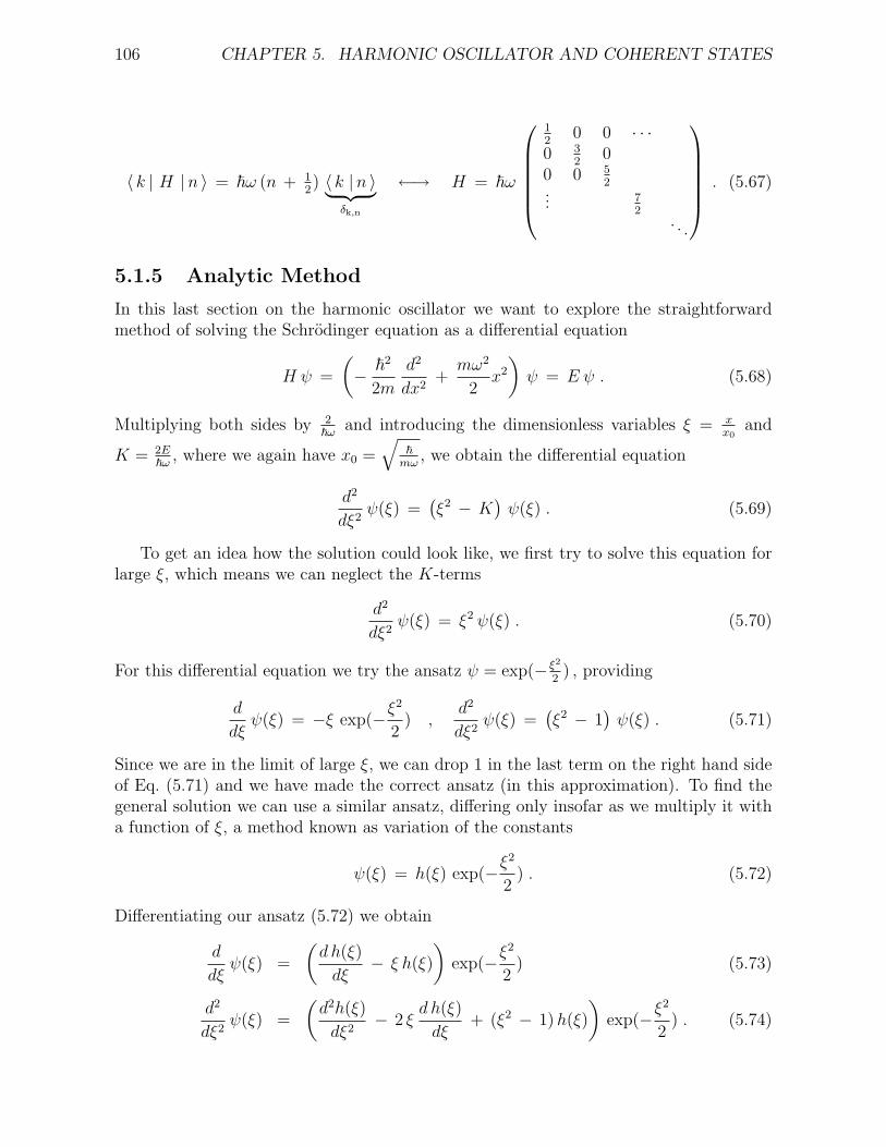
106 CHAPTER 5. HARMONIC OSCILLATOR AND COHERENT STATES
〈 k | H |n 〉 = ~ω (n + 12) 〈 k |n 〉︸ ︷︷ ︸
δk,n
←→ H = ~ω
12
0 0 · · ·0 3
20
0 0 52
... 72
. . .
. (5.67)
5.1.5 Analytic Method
In this last section on the harmonic oscillator we want to explore the straightforwardmethod of solving the Schrodinger equation as a differential equation
H ψ =
(− ~2
2m
d2
dx2+mω2
2x2
)ψ = E ψ . (5.68)
Multiplying both sides by 2~ω and introducing the dimensionless variables ξ = x
x0and
K = 2E~ω , where we again have x0 =
√~mω
, we obtain the differential equation
d2
dξ2ψ(ξ) =
(ξ2 − K
)ψ(ξ) . (5.69)
To get an idea how the solution could look like, we first try to solve this equation forlarge ξ, which means we can neglect the K-terms
d2
dξ2ψ(ξ) = ξ2 ψ(ξ) . (5.70)
For this differential equation we try the ansatz ψ = exp(− ξ2
2) , providing
d
dξψ(ξ) = −ξ exp(−ξ
2
2) ,
d2
dξ2ψ(ξ) =
(ξ2 − 1
)ψ(ξ) . (5.71)
Since we are in the limit of large ξ, we can drop 1 in the last term on the right hand sideof Eq. (5.71) and we have made the correct ansatz (in this approximation). To find thegeneral solution we can use a similar ansatz, differing only insofar as we multiply it witha function of ξ, a method known as variation of the constants
ψ(ξ) = h(ξ) exp(−ξ2
2) . (5.72)
Differentiating our ansatz (5.72) we obtain
d
dξψ(ξ) =
(d h(ξ)
dξ− ξ h(ξ)
)exp(−ξ
2
2) (5.73)
d2
dξ2ψ(ξ) =
(d2h(ξ)
dξ2− 2 ξ
d h(ξ)
dξ+ (ξ2 − 1)h(ξ)
)exp(−ξ
2
2) . (5.74)
5.2. COHERENT STATES 107
On the other hand we know the second derivative of ψ from the Schrodinger equation(5.69), leading to a differential equation for the function h(ξ)
d2h(ξ)
dξ2− 2 ξ
d h(ξ)
dξ+ (K − 1)h(ξ) = 0 , (5.75)
which can be solved by a power series ansatz. We are not computing this here, but directthe interested reader to a lecture and/or book about differential equations4. Equation(5.75) is the differential equation for the so called Hermite polynomials Hn, thus wereplace our function by
h(ξ) → Hn(ξ) , n = 0, 1, 2, · · · (5.76)
where (K − 1) = 2n or K = 2E~ω = 2n+ 1 respectively. With this substitution we directly
find the energy levels of the harmonic oscillator, as calculated earlier in Eq. (5.30)
En = ~ω (n + 12) . (5.77)
With the help of the Hermite polynomials we can now also give the exact expressionfor the eigenfunctions of the harmonic oscillator
ψn =1√
2n(n!)
(mωπ~
)14Hn(
x
x0
) exp(− x2
2x20
) . (5.78)
The Hermite Polynomials can be easiest calculated with the Formula of Rodrigues
Hn(x) = (−1)n ex2
(dn
dxne−x
2
). (5.79)
To give some examples we list some of the first Hermite Polynomials
H0(x) = 1 , H1(x) = 2x , H2(x) = 4x2 − 2
H3(x) = 8x3 − 12x , H4(x) = 16x4 − 48x2 + 12 . (5.80)
A last interesting property is the orthogonality relation of the Hermite Polynomials
∞∫−∞
dx Hm(x) Hn(x) e−x2
=√π 2n (n!) δmn . (5.81)
5.2 Coherent States
Coherent states play an important role in quantum optics, especially in laser physics andmuch work was performed in this field by Roy J. Glauber who was awarded the 2005Nobel prize for his contribution to the quantum theory of optical coherence. We will tryhere to give a good overview of coherent states of laser beams. The state describing alaser beam can be briefly characterized as having
4See for example [14].
108 CHAPTER 5. HARMONIC OSCILLATOR AND COHERENT STATES
1. an indefinite number of photons,
2. but a precisely defined phase,
in contrast to a state with fixed particle number, where the phase is completely random.
There also exists an uncertainty relation describing this contrast, which we will plainlystate here but won’t prove. It can be formulated for the uncertainties of amplitude andphase of the state, where the inequality reaches a minimum for coherent states, or, as wewill do here, for the occupation number N and the phase Φ 5
∆N ∆(sin Φ) ≥ 1
2cos Φ , (5.82)
which, for small Φ, reduces to
∆N ∆Φ ≥ 1
2. (5.83)
5.2.1 Definition and Properties of Coherent States
Since laser light has a well-defined amplitude – in contrast to thermal light which is astatistical mixture of photons – we will define coherent states as follows:
Definition 5.3 A coherent state |α 〉 , also called Glauber state,is defined as eigenstate of the amplitude operator,the annihilation operator a , with eigenvalues α ∈ C
a |α 〉 = α |α 〉 .
Since a is a non-hermitian operator the phase α = |α| eiϕ ∈ C is a complex numberand corresponds to the complex wave amplitude in classical optics. Thus coherent statesare wave-like states of the electromagnetic oscillator.
Properties of coherent states:
Let us study the properties of coherent states.
Note: The vacuum | 0 〉 is a coherent state with α = 0 .
Mean energy:
〈H 〉 = 〈α | H |α 〉 = ~ω 〈α | a†a + 12|α 〉 = ~ω ( |α|2 + 1
2) . (5.84)
The first term on the right hand side represents the classical wave intensity and the secondthe vacuum energy.
5See for example [15].

5.2. COHERENT STATES 109
Next we introduce the phase shifting operator
U(θ) = e−iθN , (5.85)
where N represents the occupation number operator (see Definition 5.2). Then we have
U †(θ) aU(θ) = a e−iθ or U(θ) aU †(θ) = a eiθ , (5.86)
i.e. U(θ) gives the amplitude operator a phase shift θ.
Proof: The l.h.s. ddθU †(θ) aU(θ) = i U †(θ) [N, a]U(θ) = −i U †(θ) aU(θ) and the
r.h.s. ddθa e−iθ = −i a e−iθ obey the same differential equation.
The phase shifting operator also shifts the phase of the coherent state
U(θ) |α 〉 =∣∣α e−iθ ⟩ . (5.87)
Proof: Multiplying Definition 5.3 with the operator U from the left and inserting theunitarian relation U † U = 1 on the l.h.s we get
U aU †︸ ︷︷ ︸a eiθ
U |α 〉 = αU |α 〉
⇒ aU |α 〉 = α e−iθ U |α 〉 . (5.88)
Denoting U |α 〉 =∣∣α′ ⟩ we find from Definition 5.3 that a
∣∣α′ ⟩ = α′ ∣∣α′ ⟩ and thus
α′= α e−iθ , q.e.d.
Now we want to study the coherent states more accurately. In order to do so weintroduce the so called displacement operator which generates the coherent states, similarto how the creation operator a†, see Eq. (5.58), creates the occupation number states |n 〉.
Definition 5.4 The displacement operator D(α) is defined by
D(α) = eαa†−α∗a
where α = |α| eiϕ ∈ C is a complex number and a†
and a are the creation - and annihilation - operators.
The displacement operator is an unitary operator, i.e. D†D = 1 and we can alsorewrite it using Eq. (2.72). To use this equation we have to ensure that the commutators[ [A , B ] , A ] and [ [A , B ] , B ] vanish, where A = α a† and B = α∗a . We thereforestart by calculating the commutator of A and B
[A , B ] =[α a† , α∗a
]= αα∗
[a† , a
]︸ ︷︷ ︸−1
= − |α|2 . (5.89)
110 CHAPTER 5. HARMONIC OSCILLATOR AND COHERENT STATES
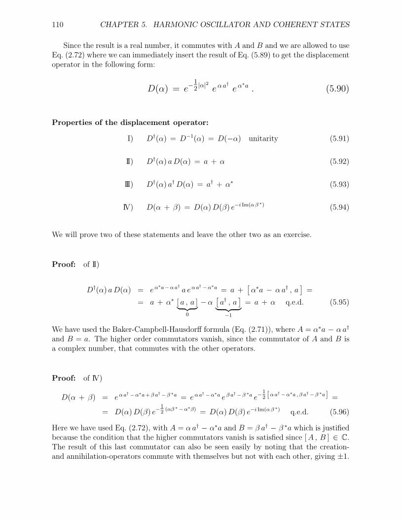
Since the result is a real number, it commutes with A and B and we are allowed to useEq. (2.72) where we can immediately insert the result of Eq. (5.89) to get the displacementoperator in the following form:
D(α) = e−12 |α|
2
eαa†eα∗a . (5.90)
Properties of the displacement operator:
I) D†(α) = D−1(α) = D(−α) unitarity (5.91)
II) D†(α) aD(α) = a + α (5.92)
III) D†(α) a†D(α) = a† + α∗ (5.93)
IV) D(α + β) = D(α)D(β) e−i Im(αβ ∗) (5.94)
We will prove two of these statements and leave the other two as an exercise.
Proof: of II)
D†(α) aD(α) = eα∗a−αa† a eαa
†−α∗a = a +[α∗a − α a† , a
]=
= a + α∗ [ a , a ]︸ ︷︷ ︸0
−α[a† , a
]︸ ︷︷ ︸−1
= a + α q.e.d. (5.95)
We have used the Baker-Campbell-Hausdorff formula (Eq. (2.71)), where A = α∗a − α a†
and B = a. The higher order commutators vanish, since the commutator of A and B isa complex number, that commutes with the other operators.
Proof: of IV)
D(α + β) = eαa†−α∗a+β a†−β ∗a = eαa
†−α∗a eβ a†−β ∗a e−
12 [αa†−α∗a , β a†−β ∗a ] =
= D(α)D(β) e−12
(αβ ∗−α∗β) = D(α)D(β) e−i Im(αβ ∗) q.e.d. (5.96)
Here we have used Eq. (2.72), with A = α a† − α∗a and B = β a† − β ∗a which is justifiedbecause the condition that the higher commutators vanish is satisfied since [A , B ] ∈ C.The result of this last commutator can also be seen easily by noting that the creation-and annihilation-operators commute with themselves but not with each other, giving ±1.

5.2. COHERENT STATES 111
With this knowledge about the displacement operator we can now create coherentstates.
Theorem 5.2 The coherent state |α 〉 is generated from the vacuum | 0 〉 by
the displacement operator D(α)
|α 〉 = D(α) | 0 〉 .
The ”vacuum” | 0 〉 is the ground state with occupation number n = 0, which is definedby a | 0 〉 = 0, see also Eq. (5.18).
Proof: Applying a negative displacement to |α 〉 we find from properties (5.91) and(5.92) that
aD(−α) |α 〉 = D(−α) D†(−α) aD(−α)︸ ︷︷ ︸a−α
|α 〉
⇒ aD(−α) |α 〉 = D(−α)(a− α) |α 〉 = 0 . (5.97)
The r.h.s. vanishes because of Definition 5.3. This implies that D(−α) |α 〉 is the vacuumstate | 0 〉
D(−α) |α 〉 = | 0 〉 ⇒ |α 〉 = D(α) | 0 〉 q.e.d. (5.98)
On the other hand, we also could use Theorem 5.2 as a definition of the coherent statesthen our Definition 5.3 would follow as a theorem.
Proof:
D(α)D†(α)︸ ︷︷ ︸1
a |α 〉 = D(α) D†(α) aD(α)︸ ︷︷ ︸a+α
| 0 〉 = D(α)
a | 0 〉︸ ︷︷ ︸0
+α | 0 〉
=
= αD(α) | 0 〉 = α |α 〉⇒ a |α 〉 = α |α 〉 q.e.d. (5.99)
The meaning of our Definition 5.3 becomes apparent when describing a coherent pho-ton beam, e.g. a laser beam. The state of the laser remains unchanged if one photon isannihilated, i.e. if it is detected.
112 CHAPTER 5. HARMONIC OSCILLATOR AND COHERENT STATES
Expansion of coherent state in Fock space: The phase |α 〉 describes the waveaspect of the coherent state. Next we want to study the particle aspect, the states in Fockspace. A coherent state contains an indefinite number of photons, which will be evidentfrom the expansion of the coherent state |α 〉 into the CONS of the occupation numberstates |n 〉 . Let us start by inserting the completeness relation of the occupationnumber states
|α 〉 =∑n
|n 〉 〈n | α 〉 . (5.100)
Then we calculate the transition amplitude 〈n | α 〉 by using Definition 5.3, where wemultiply the whole eigenvalue equation with 〈n | from the left
〈n | a |α 〉 = 〈n | α |α 〉 . (5.101)
Using the adjoint of relation (5.59) we rewrite the left side of Eq. (5.101)
a† |n 〉 =√n + 1 |n + 1 〉 ⇒ 〈n | a =
√n + 1 〈n + 1 | (5.102)
√n + 1 〈n + 1 |α 〉 = α 〈n |α 〉 , (5.103)
and replace the occupation number n with n− 1 to obtain
〈n |α 〉 =α√n〈n − 1 |α 〉 . (5.104)
By iterating the last step, i.e. again replacing n with n− 1 in Eq. (5.104) and reinsertingthe result on the right hand side, we get
〈n |α 〉 =α2√
n(n − 1)〈n − 2 |α 〉 = · · · =
αn√n!〈 0 |α 〉 , (5.105)
which inserted into the expansion of Eq. (5.100) results in
|α 〉 = 〈 0 |α 〉∞∑n=0
αn√n!|n 〉 . (5.106)
The remaining transition amplitude 〈 0 |α 〉 can be calculated in two different ways,first with the normalization condition and second with the displacement operator. For thesake of variety we will use the second method here and leave the other one as an exercise
〈 0 |α 〉 = 〈 0 | D(α) | 0 〉 Eq. (5.90)= e−
12|α|2 〈 0 | eαa† eα∗a | 0 〉 . (5.107)
We expand the exponentials of operators in the scalar product into their Taylor series
〈 0 | eαa† eα∗a | 0 〉 = 〈 0 | (1 + α a† + · · · )(1 + α∗ a + · · · ) | 0 〉 = 1 , (5.108)
and we let the left bracket act to the left on the bra and right bracket to the right on theket. In this way we can both times use the vacuum state property a | 0 〉 = 0 to eliminateall terms of the expansion except the first. Therefore the transition amplitude is given by
〈 0 |α 〉 = e−12|α|2 , (5.109)
5.2. COHERENT STATES 113
and we can write down the coherent state in terms of an exact expansion in Fock space
|α 〉 = e−12 |α|
2∞∑n=0
αn√n!|n 〉 = e−
12 |α|
2∞∑n=0
(α a†)n
n!| 0 〉 . (5.110)
Probability distribution of coherent states: We can subsequently analyze theprobability distribution of the photons in a coherent state, i.e. the probability of detectingn photons in a coherent state |α 〉, which is given by
P (n) = |〈n |α 〉|2 =|α|2n e−|α|2
n!. (5.111)
By noting, that the mean photon number is determined by the expectation value ofthe particle number operator
n = 〈α | N |α 〉 = 〈α | a†a |α 〉 Def. 5.3= |α|2 , (5.112)
we can rewrite the probability distribution to get
P (n) =nn e−n
n!, (5.113)
which is a Poissonian distribution.
Remarks: First, Eq. (5.112) represents the connection between the mean photonnumber – the particle view – and the complex amplitude squared, the intensity of thewave – the wave view.
Second, classical particles obey the same statistical law, the Poisson formula (5.111),when they are taken at random from a pool with |α|2 on average. Counting thereforethe photons in a coherent state, they behave like randomly distributed classical particles,which might not be too surprising since coherent states are wave-like. Nevertheless, it’samusing that the photons in a coherent state behave like the raisins in a Gugelhupf 6, whichhave been distributed from the cook randomly with |α|2 on average per unit volume. Thenthe probability of finding n raisins per unit volume in the Gugelhupf follows precisely law(5.111).
Scalar product of two coherent states: From Theorem 4.3 we can infer some im-portant properties of the particle number states, which are the eigenstates of the particlenumber operator N = a†a. Since this operator is hermitian, the eigenvalues n are real andthe eigenstates |n 〉 are orthogonal. But the coherent states are eigenstates of the annihi-lation operator a, which is surely not hermitian and as we already know, the eigenvaluesα are complex numbers. Therefore we cannot automatically assume the coherent states
6A traditional Austrian birthday cake.

114 CHAPTER 5. HARMONIC OSCILLATOR AND COHERENT STATES
to be orthogonal, but have to calculate their scalar product, using again Theorem 5.2 andEq. (5.90)
〈 β |α 〉 = 〈 0 | D†(β)D(α) | 0 〉 = 〈 0 | e−β a† eβ ∗ a eαa† e−α∗a | 0 〉 e−12
(|α|2 + |β|2) . (5.114)
We now use the same trick as in Eq. (5.108), i.e., expand the operators in theirTaylor series, to see that the two ”outer” operators e−β a
†= (1− β a† + · · · ) and e−α
∗a =(1−α∗a+ · · · ), acting to left and right respectively, annihilate the vacuum state, save forthe term ”1” and we can thus ignore them. We then expand the remaining operators aswell and consider their action on the vacuum
〈 0 | (1 + β ∗a +1
2!(β ∗a)2 + · · · ) (1 + α a† +
1
2!(α a†)2 + · · · ) | 0 〉 (5.115)
= ( · · · + 〈 2 | 1
2!
√2! (β ∗)2 + 〈 1 | β ∗ + 〈 0 | ) ( | 0 〉 + α | 1 〉 +
1
2!
√2!α2 | 2 〉 + · · · ) .
Using the orthogonality of the particle number states 〈n |m 〉 = δnm we get
〈 β |α 〉 = e−12
(|α|2 + |β|2) ( 1 + αβ ∗ +1
2!(αβ ∗)2 + · · · ) = e−
12
(|α|2 + |β|2) +αβ ∗ . (5.116)
We further simplify the exponent, by noting that
|α − β |2 = (α − β)(α∗ − β ∗) = |α|2 + |β|2 − αβ ∗ − α∗β , (5.117)
and we can finally write down the transition probability in a compact way
| 〈 β |α 〉 |2 = e−|α−β |2
. (5.118)
That means, the coherent states indeed are not orthogonal and their transition prob-ability only vanishes in the limit of large differences |α − β | 1.
Completeness of coherent states: Although the coherent states are not orthog-
onal, it is possible to expand coherent states in terms of a complete set of states. The
completeness relation for the coherent states reads
1
π
∫d 2α |α 〉 〈α | = 1 . (5.119)
In fact, the coherent states are ”overcomplete”, which means that, as a consequenceof their nonorthogonality, any coherent state can be expanded in terms of all the othercoherent states. So the coherent states are not linearly independent
| β 〉 =1
π
∫d 2α |α 〉 〈α | β 〉 =
1
π
∫d 2α |α 〉 e−
12
(|α|2 + |β|2) +αβ ∗ . (5.120)
5.2. COHERENT STATES 115
Proof of completeness:
1
π
∫d 2α |α 〉 〈α | Eq. (5.110)
=1
π
∑n,m
1√n!m!
|n 〉 〈m |∫d 2α e−|α|
2
αn(α∗)m . (5.121)
The integral on the right hand side of Eq. (5.121) can be solved using polar coordinatesα = |α|eiϕ = r eiϕ
∫d 2α e−|α|
2
αn(α∗)m =
∞∫0
r dr e−r2
rn+m
2π∫0
dϕ ei(n−m)ϕ
︸ ︷︷ ︸2π δnm
= 2π
∞∫0
r dr e−r2
r2n .
(5.122)Substituting r2 = t, 2rdr = dt to rewrite the integral
2
∞∫0
r dr e−r2
r2n =
∞∫0
e−t tn dt = Γ(n + 1) = n! , (5.123)
we recover the exact definition of the Gamma function, see [13, 14]. With this we canfinally write down the completeness relation
1
π
∫d 2α |α 〉 〈α | =
1
π
∑n
1
n!|n 〉 〈n | π n! =
∑n
|n 〉 〈n | = 1 q.e.d. (5.124)
5.2.2 Coordinate Representation of Coherent States
Recalling the coherent state expansion from Eq. (5.110)
|α 〉 = e−12|α|2
∞∑n=0
αn√n!|n 〉 = e−
12|α|2
∞∑n=0
(α a†)n
n!| 0 〉 , (5.125)
and the coordinate representation of the harmonic oscillator states (Eq. (5.78))
ψn(x) = 〈x |n 〉 = ψn(x) =1√
2n(n!)√πx0
Hn(ξ) e−ξ2
2 (5.126)
ψ0(x) = 〈x | 0 〉 = ψ0(x) =1√√πx0
e−ξ2
2 , (5.127)
where ξ = xx0
and x0 =√
~mω
, we can easily give the coordinate representation of the
coherent states
〈x |α 〉 = φα(x) = e−12|α|2
∞∑n=0
αn√n!ψn(x) = e−
12|α|2
∞∑n=0
(α a†)n
n!ψ0(x) . (5.128)
116 CHAPTER 5. HARMONIC OSCILLATOR AND COHERENT STATES
Time evolution: Let’s first take a look at the time evolution of the harmonic oscillatorstates and at the end we recall Theorem 4.1 and Definition 4.1. Using the harmonicoscillator energy (Eq. (5.77)) we easily get
ψn(t, x) = ψn(x) e−i~Ent = ψn(x) e−in ωt e−
iωt2 . (5.129)
We are then in the position to write down the time evolution of the coherent state
φα(t, x) = e−12|α|2 e−
iωt2
∞∑n=0
(α e−iωt)n√n!
ψn(x) . (5.130)
With a little notational trick, i.e. making the label α time dependent α(t) = α e−iωt ,
we can bring Eq. (5.130) into a more familiar form
φα(t, x) = φα(t)(x) e−iωt2 , (5.131)
which we can identify as a solution of the time dependent Schrodinger equation.
Expectation value of x for coherent states: Subsequently, we want to comparethe motion of coherent states to that of the quantum mechanical (and classical) harmonicoscillator, which we will do by studying the expectation value of the position operator.For the quantum mechanical case we have already calculated the mean position, whichdoes not oscillate (see Eq. (5.34))
〈x 〉oscillator = 0 . (5.132)
Recalling the expression of x in terms of creation and annihilation operators, Eq. (5.5),and the eigenvalue equation of the annihilation operator, Definition 5.3, we can easilycompute the expectation value of the position for the coherent states
〈x 〉coherent =⟨φα(t)
∣∣ x ∣∣φα(t)
⟩=
x0√2
⟨φα(t)
∣∣ a + a†∣∣φα(t)
⟩= (5.133)
=x0√
2(α(t) + α∗(t)) =
√2x0 Re(α(t)) =
√2x0 |α| cos(ωt − ϕ) ,
where we used α(t) = α e−iωt = |α| e−i(ωt−ϕ). To summarize the calculation, we conclude
that the coherent state, unlike the quantum mechanical harmonic oscillator, does oscillate,
similar to its classical analogue
〈x 〉coherent =√
2x0 |α| cos(ωt − ϕ) . (5.134)

5.2. COHERENT STATES 117
Coordinate representation in terms of displacement operator: In this sectionwe want to express and study the coordinate representation of coherent states via thedisplacement operator D
φα(x) = 〈x |α 〉 = 〈x | D(α) | 0 〉 = 〈x | eαa†−α∗a | 0 〉 . (5.135)
To simplify further calculations we now rewrite the creation and annihilation operatorsfrom Definition 5.1 in terms of the dimensionless variable ξ = x
x0,
a = 1√2(ξ +
d
dξ) , a† = 1√
2(ξ − d
dξ) . (5.136)
This rewritten operators (5.136) we insert into the exponent of the displacement operatorfrom Eq. (5.135)
α a† − α∗a =α√2
(ξ − d
dξ) − α∗√
2(ξ +
d
dξ) =
=ξ√2
(α − α∗︸ ︷︷ ︸2i Im(α)
) − 1√2
d
dξ(α + α∗︸ ︷︷ ︸
2 Re(α)
) =
=√
2 i Im(α) ξ −√
2 Re(α)d
dξ, (5.137)
and get for the wavefunction (5.135) the following expression
φα(x) = 〈x |α 〉 = e√
2 i Im(α) ξ−√
2 Re(α) ddξ ψ0(ξ) , (5.138)
where ψ0 is the harmonic oscillator ground state (Eq. (5.127)).
The time dependent version follows outright
φα(t, x) = φα(t) e− iωt
2 = 〈x |α(t) 〉 e−iωt2 = e−
iωt2 〈x | eα(t) a†−α∗(t)a | 0 〉
⇒ φα(t, x) = e−iωt2 e√
2 i Im(α(t)) ξ−√
2 Re(α(t)) ddξ ψ0(ξ) . (5.139)
On the other hand, as a check, we can also arrive at this result by starting from ex-pansion (5.125), where we interpret the sum over n as the power series for the exponentialmap, i.e.
φα(t, x) = e−12|α|2 e−
iωt2
∞∑n=0
(α(t) a†)n
n!ψ0(x) = e−
12|α|2 e−
iωt2 eα(t) a† ψ0(x) . (5.140)

118 CHAPTER 5. HARMONIC OSCILLATOR AND COHERENT STATES
To show that this result is the same as Eq. (5.139) we simply calculate
eα(t) a†−α∗(t) a ψ0(x)Eq. (2.72)
= eα(t) a† e−α∗(t) a e
12αα∗
−1︷ ︸︸ ︷[a† , a
]ψ0(x) =
= e−12|α|2 eα(t) a† (1 − α∗(t)
−→ 0a + · · · ) ψ0(x) =
= e−12|α|2 eα(t) a† ψ0(x) , (5.141)
where we once again used the fact, that the action of the annihilation operator on theground state vanishes. Inserting the result into Eq. (5.140) we get
φα(t, x) = e−iωt2 eα(t) a†−α∗(t) a ψ0(x) . (5.142)
Explicit calculation of the wave function: Our aim is now to explicitly compute
the wave function from expression (5.138). We first state the result and derive it in the
following
φα(t, x) =1√x0√πe−
iωt2 e√
2 i Im(α(t)) ξ−√
2 Re(α(t)) ddξ e−
ξ2
2
=1√x0√πe−
iωt2 e√
2α(t) ξ− ξ2
2 −Re(α(t))α(t) . (5.143)
Proof: Let us now perform the explicit calculation. That means, we apply the
differential operator7 eD = e√
2 i Im(α(t)) ξ−√
2 Re(α(t))ddξ to the ground state of the harmonic
oscillator ψ0(ξ) = 1√x0√πe−
ξ2
2 , but we will only consider the linear and quadratic term of
the operator expansion, as sketched in Eq. (5.144)
eD e−ξ2
2 = (1 + D +1
2!D2 + · · · ) e−
ξ2
2 , (5.144)
linear term: D e−ξ2
2 =(√
2 i Im(α(t)) ξ −√
2 Re(α(t) ddξ
)e−
ξ2
2
=(√
2 i Im(α(t)) ξ +√
2 Re(α(t) ξ)e−
ξ2
2
=√
2 ξ (Re(α(t)) + i Im(α(t)))︸ ︷︷ ︸α(t)
e−ξ2
2
=√
2α(t) ξ e−ξ2
2 , (5.145)
7The operator D, which is a notation to shorten the cumbersome calculations, is not to be confusedwith the displacement operator D.
5.2. COHERENT STATES 119
quadratic term:
D2 e−ξ2
2 =√
2α(t)D ξ e−ξ2
2 (5.146)
=√
2α(t)(√
2 i Im(α(t)) ξ −√
2 Re(α(t)) ddξ
)ξ e−
ξ2
2
=(2α(t) i Im(α(t)) ξ2 − 2α(t) Re(α(t)) + 2α(t) Re(α(t)) ξ2
)e−
ξ2
2
= (2α(t) (Re(α(t)) + i Im(α(t)))︸ ︷︷ ︸α(t)
ξ2 − 2α(t) Re(α(t))) e−ξ2
2 .
Inserting the results of Eq. (5.145) and Eq. (5.146) into the expansion (5.144) we get
eD e−ξ2
2 = (1 +√
2α(t)ξ − α(t) Re(α(t))︸ ︷︷ ︸linear term
+2α(t)α(t) ξ2
2!+ · · · ) e−
ξ2
2 , (5.147)
where we can already identify the linear term and the first part of the quadratic term inthe end result of the expansion. Finally, rewriting the whole expansion as exponential
function and including the factor e−ξ2
2 , we arrive at the proposed result of Eq. (5.143).
Probability distribution of the wave packet: As last computation in this sectionwe want to study the probability density of the wave function of the coherent state, thuswe take the modulus squared of expression (5.143)
|φα(t, x)|2 = φ∗α φα(t, x)
=1
x0
√πe−ξ
2 +√
2
2Re(α(t))︷ ︸︸ ︷(α∗ + α) ξ−Re(α(t))
2Re(α(t))︷ ︸︸ ︷(α∗ + α)
=1
x0
√πe−(ξ−
√2 Re(α(t)))
2
=1
x0
√πe−(ξ−
√2 |α| cos(ωt−ϕ))
2
. (5.148)
Recalling the result for the expectation value (the mean value) of the position (Eq. (5.134))
and our choice of ξ = xx0
we finally find the probability density
|φα(t, x)|2 =1
x0√π
exp
(−(x − 〈 x 〉 (t))2
x20
), (5.149)
which is a Gaussian distribution with constant width.
Result: The coherent states are oscillating Gaussian wave packets with constantwidth in a harmonic oscillator potential, i.e., the wave packet of the coherent state isnot spreading (because all terms in the expansion are in phase). It is a wave packetwith minimal uncertainty. These properties make the coherent states the closest quantummechanical analogue to the free classical single mode field. For an illustration see Fig. 5.3.

120 CHAPTER 5. HARMONIC OSCILLATOR AND COHERENT STATES
Figure 5.3: Coherent state: The probability density of the coherent state is a Gaussiandistribution, whose center oscillates in a harmonic oscillator potential. Due to its being asuperposition of harmonic oscillator states, the coherent state energy is not restricted tothe energy levels ~ω(n + 1
2) but can have any value (greater than the zero point energy).