96

CHAPTER 6

HANDHELD ANTENNA ARRAY TESTBED (HAAT)

6.1 Introduction

An experiment system was developed to measure diversity combining and

adaptive beamforming performance using various array configurations and combining

algorithms. This chapter describes the Handheld Antenna Array Testbed (HAAT) system

and associated hardware and software. The HAAT was developed based on the

requirements of planned antenna diversity and adaptive beamforming experiments. Key

features of this system include portability and ability to test hand-held antenna

configurations in typical microcellular and peer-to-peer communication scenarios.

This chapter begins with an overview of the HAAT system, followed by

descriptions of the system components. The components include transmitters, a linear

positioning system, two- and four-channel receivers and data loggers, data processing

hardware, and the software used to process data and evaluate performance of diversity

combining and adaptive beamforming. Sample graphs of the data processing software

outputs are shown.

6.2 System Overview

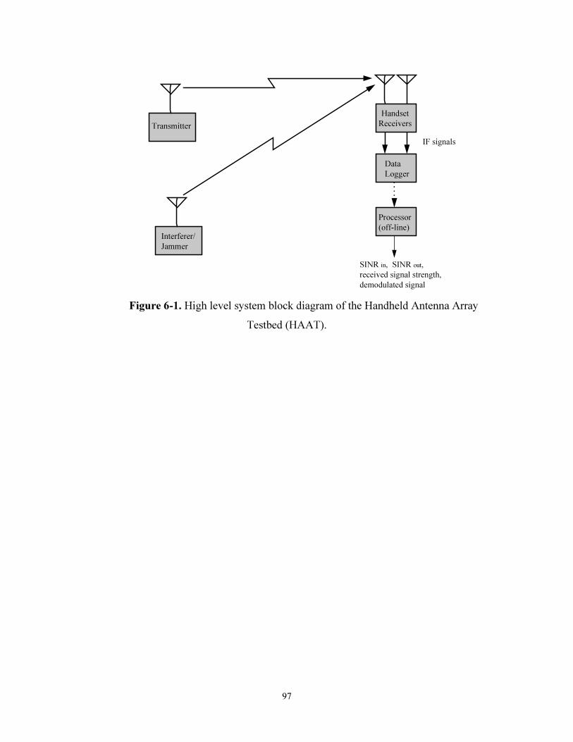
A high-level block diagram of the HAAT is shown in Fig. 6-1. The HAAT

operates at 2.05 GHz. CW signals are transmitted from one or two transmitters. Data are

collected using either a two- or a four-channel portable receiver system. The data are

analyzed off line to allow comparison of different combining techniques. Figure 6-2

shows the two-channel receiver/data logger and data processing system. Each of the

components of the HAAT is described in this section. More details on the software are

included in the Appendices.

97

Transmitter

Interferer/

Jammer

Handset

Receivers

Data

Logger

Processor

(off-line)

SINR in, SINR out,

received signal strength,

demodulated signal

IF signals

Figure 6-1. High level system block diagram of the Handheld Antenna Array

Testbed (HAAT).

Figure 6-2. Block diagram of the two-channel HAAT receiver/data logger and data processing system

Receiver

DAT recorder

Antenna

ArrayDAT recorder

Computer

SINR improvement,

diversity gain, etc.

Processing Software

• Quadrature

Downconversion

• Adaptive/

Diversity

Combining

• Performance

Measurement

Digital Audio Card

Audio Software

RF:

2.050 GHz

Baseband:

0-24 kHz

LO

98

99

6.3 Transmitters

The testbed uses one or two transmitters. For diversity measurements only one of

the transmitters is used. Both transmitters are used when interference rejection

measurements are performed to evaluate adaptive beamforming performance. Either

source can be considered as transmitting the desired signal. The other source is then an

interfering signal. The transmitters use the architecture depicted in Fig. 6-3. Table 6-1

lists the major transmitter components. The transmitters are typically mounted on tripods

and operate from fixed positions but are transportable and run on batteries for use in the

field. Additional transmitters can be added as needed. The transmitters transmit

continuous wave (CW) signals at 2.05 GHz. The transmitter frequencies are offset by

about 1 kHz so that the signals can be distinguished, and both signals fall within the

bandwidth of the receiver unit.

OCXO

50 MHz

Adjustment

Phase-

locked

multiplier

Figure 6-3. Block diagram of a HAAT transmitter

Table 6-1. Major Transmitter Components

Component Manufacturer Part Number Quantity per

Transmitter

Reference Oscillator Hewlett Packard 1

Signal Source NOVA SOURCE 20002500-100X 1

Power Amplifier MINI CIRCUITS ZFL 2500 VH 1

Batteries (6V gelcells)

Power Patrol SLA0905 3

6.4 Linear Positioning System

A portable positioning system is used for controlled measurements. The

positioning system is shown in Fig. 6-4 and consists of a non-metallic track

approximately 3 m in length. The major positioner components are listed in Table 6-2.

100

The useable length of the track is about 2.8 m (approximately 20 wavelengths at 2.05

GHz). The receiver is mounted on a carriage that is moved along the track at a constant

speed, using a stepper motor, while measurements are conducted. The track is mounted

on an adjustable tripod to allow use on any terrain. An electronic level is used to adjust

the tripod to level the track.

Figure 6-4. Positioning system for controlled tests

Table 6-2. Major Positioning System Components

Component Manufacturer Part Number Quantity

Motor Superior Electric M061-FD-427U 1

Motor Controller J. R. Nealy 1

Motor ControllerBoard

Modern Technology MTSD-V1 1

Battery (6V gelcell)

Power Patrol SLA0905 1

Tripod 1

Track J. R. Nealy 1

Carriage J. R. Nealy 1

6.5 Two-Channel Handheld Receiver Unit and Data Logger

The handheld receiver unit consists of a box having the approximate size and

shape of a handheld radio and includes antennas, receivers, and a portable DAT recorder

(a Sony TCD-D8), used to log data. Two antennas, each connected to a separate receiver,

are mounted on the box. The receiver IF outputs are connected to the DAT. The entire

receiver unit is portable so that it can be carried by an operator, and is rugged enough that

it can be used to perform experiments in a wide variety of locations and conditions.

101

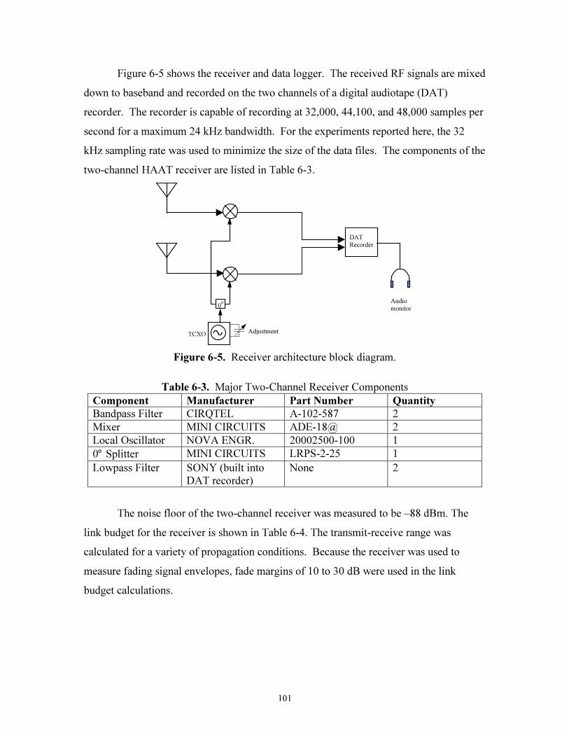
Figure 6-5 shows the receiver and data logger. The received RF signals are mixed

down to baseband and recorded on the two channels of a digital audiotape (DAT)

recorder. The recorder is capable of recording at 32,000, 44,100, and 48,000 samples per

second for a maximum 24 kHz bandwidth. For the experiments reported here, the 32

kHz sampling rate was used to minimize the size of the data files. The components of the

two-channel HAAT receiver are listed in Table 6-3.

TCXO

DAT

Recorder

0o

Adjustment

Audio

monitor

Figure 6-5. Receiver architecture block diagram.

Table 6-3. Major Two-Channel Receiver Components

Component Manufacturer Part Number Quantity

Bandpass Filter CIRQTEL A-102-587 2

Mixer MINI CIRCUITS ADE-18@ 2

Local Oscillator NOVA ENGR. 20002500-100 1

0° Splitter MINI CIRCUITS LRPS-2-25 1

Lowpass Filter SONY (built intoDAT recorder)

None 2

The noise floor of the two-channel receiver was measured to be –88 dBm. The

link budget for the receiver is shown in Table 6-4. The transmit-receive range was

calculated for a variety of propagation conditions. Because the receiver was used to

measure fading signal envelopes, fade margins of 10 to 30 dB were used in the link

budget calculations.

102

Table 6-4. Link Budget for the Two-Channel HAAT Receiver

Transmitter power, dBm 27.00 27.00 27.00

Transmitter cable losses, dB 2.00 2.00 2.00

Gain of transmitting antenna, dBi 2.15 2.15 2.15

EIRP, dBm 27.15 27.15 27.15

Gain of receiving antenna, dBi 2.15 2.15 2.15

Receiver cable losses, dB 2.00 2.00 2.00

Receiver noise floor, dBm -88.00 -88.00 -88.00

Minimum mean SNR (fade margin), dB 10.00 20.00 30.00

Maximum allowable path loss, dB 105.30 95.30 85.30

Wavelength in m at 2.05 GHz 0.1463 0.1463 0.1463

Path loss in dB at 1 m, 2.05 GHz 38.7 38.7 38.7

Maximum path loss beyond 1m 66.6 56.6 46.6

Maximum range in m, free space, n=2 2144 678 214

Maximum range in m, n=3 166 77 36

Maximum range in m, n=4 46 26 15

6.6 Four-Channel HAAT Receiver and Data Logger

Figure 6-6 shows a block diagram of the 4-channel receiver, as well as a high-

level view of the data collection and processing. Each antenna is connected directly to a

mixer and the received RF signal at 2.05 GHz is mixed down directly to baseband.

Filtering is performed by the anti-aliasing filters internal to the two portable digital audio

tape machines that are used to record the data. This configuration results in low power

consumption. The noise figure of 28 dB is relatively high but suitable for the application.

The receiver is powered by three lead-acid gel-cell batteries that supply 18 V DC. The

receiver draws approximately 200 mA.

Figure 6-6. Block diagram of the 4-channel HAAT receiver

Receiver

DAT 1

Antenna

ArrayDAT Recorder

Computer

SINR improvement,

diversity gain, etc.

Processing Software

• Quadrature

Downconversion

• Adaptive/Diversity

Combining

• Performance

Measurement

Digital Audio Card

Audio Software

RF:

2.050 GHz

Baseband:

0-24 kHz

LO

DAT 2Synch.

Pulse

103

104

6.6.1 Calibration of the four-channel receiver

The receiver was calibrated using the configuration shown in Fig. 6-7. An HP

8648C signal generator was connected to two channels of the receiver using a two way

splitter. The signal generator was set to a frequency of 2.05 GHz and the output power

was varied from –130 to –30 dBm (resulting in -134 to –34 dBm into the receiver). The

two unused antenna ports were terminated in 50 Ω loads. The received signal was

recorded on a DAT as in normal operation of the receiver

2-way

splitterReceiver

DAT 1

HP 8648C

Signal Generator

DAT 2

~4 dB

loss

1

2

3

4

R

R

L

L

Figure 6-7. Block diagram of the equipment configuration used for receiver calibration.

The noise floor was calculated using the relative total signal-plus-noise power in

measurements with a known signal power. The noise floor was calculated using the

diversity combining software and was found to be –126 dBm in a 100 Hz bandwidth.

When using the adaptive beamforming software, the noise floor was determined

by the mean measured ratio of the power in the 100 Hz signal bandwidth (due to a known

input power) to the power in 100 Hz bandwidth at a frequency a few kHz removed from

the received signal. This is a close approximation of signal-to-noise ratio (SNR) and

depends on the length of the window used in the calculation. The noise floor was found

to be approximately

–122 dBm with a window of 320 samples and –125 dBm for a window of 640 samples.

The maximum power that did not overload the DAT was –36 dBm. Combined

with the noise floor measurements, this yields a dynamic range for the receiver of

between 86 and 90 dB, depending on the software that is used. This is in line with the

claimed dynamic range of 87+ dB for the digital audiotape recorder. This indicates that

quantization noise and not thermal noise is the dominant noise source in this receiver.

Using the diversity combining software, the noise figure of the receiver was calculated to

105

be 28 dB, but the receiver would have to be measured directly without using the DAT

recorder in order to calculate the noise figure accurately.

The usable dynamic range of the system is limited by the need to detect

synchronization pulses that are used to mark the beginning and end of each measurement.

This problem is described in more detail later in this section. In addition, the phase noise

due to the local oscillators in the transmitter and receiver, measured at 1kHz from the

spectral peak, is relatively high at approximately 54 dB below the peak signal power.

This limits the maximum signal-to-interference-plus-noise ratio (SINR) that can be

measured to approximately 54 dB.

A link budget was calculated using the measured noise floor and a distance-

dependent exponential path loss model. The link budget, shown in Table 6-4, includes a

fade margin of 10 to 50 dB to allow measurement of fading of the received signal or

signals. Also, the maximum interference rejection that can be measured is determined by

the fade margin.

Table 6-4. Link budget for the 4-channel HAAT receiver

Transmitter power, dBm 27.00 27.00 27.00 27.00 27.00

Transmitter cable losses, dB 1.00 1.00 1.00 1.00 1.00

Gain of transmitting antenna, dBi 2.15 2.15 2.15 2.15 2.15

EIRP, dBm 28.15 28.15 28.15 28.15 28.15

Gain of receiving antenna, dBi 2.15 2.15 2.15 2.15 2.15

Receiver cable losses, dB 1.00 1.00 1.00 1.00 1.00

Receiver noise floor, dBm -122.00 -122.00 -122.00 -122.00 -122.00

Minimum mean SNR (fade margin), dB 10.00 20.00 30.00 40.00 50.00

Maximum allowable path loss, dB 141.30 131.30 121.30 111.30 101.30

Wavelength in m at 2.05 GHz 0.1463 0.1463 0.1463 0.1463 0.1463

Path loss in dB at 1 m, 2.05 GHz 38.7 38.7 38.7 38.7 38.7

Maximum path loss beyond 1m 102.6 92.6 82.6 72.6 62.6

Maximum range in m, n=2 (free space) 135256 42772 13526 4277 1353

Maximum range in m, n=3 2635 1223 568 263 122

Maximum range in m, n=4 368 207 116 65 37

Additional measurements were performed to calibrate the receiver for phase and

power balance between channels. Measurements were performed similar to those for the

noise floor calculations. The signal generator was adjusted to provide a signal first at a

frequency close to that of the first HAAT transmitter (4 kHz offset from the receiver LO)

and then at a frequency close to that of the second HAAT transmitter (5 kHz offset from

106

the receiver LO). A power level of –74 dBm, well within the linear range of the receiver,

was used. Two channels were sampled at the same time. First, channels 1 and 2 were

measured, then channels 1 and 3, then 1 and 4. For each pair of channels, two

measurements were taken at each frequency. The cable connections to the two receiver

ports were switched between measurements to calibrate out phase and power imbalances

in the splitter. The results are shown in Table 6-5.

Table 6.5 Power and Phase Balance Between Channels of the 4-channel HAAT

Receiver.

Amplitude and PhaseBalance

Ampbal., dB

Phasebal.,degrees

Ch 2/ Ch 1, 4kHz -0.15 -9.34

Ch 2/ Ch 1, 5kHz -0.15 -9.36

Ch 3/ Ch 1, 4kHz 0.08 9.45

Ch 3/ Ch 1, 5kHz 0.09 9.44

Ch 4/ Ch 1, 4kHz 0.07 9.08

Ch 4/ Ch 1, 5kHz 0.06 9.05

In typical operation of the HAAT, synchronization pulses are inserted in the

receiver baseband output at the beginning and end of each measurement. The pulses

have two purposes. First, they mark the beginning and end of a measurement. If the

positioner is used, the pulses mark the beginning and end of the receiver’s motion.

Second, the pulses allow synchronization of data collected with two different DAT

recorders, where each DAT records two of the four channels of the receiver. The pulses

are generated by coupling the switch from the HAAT positioner motor controller to the

receiver audio output for channels 2 and 4. The resistor values in the circuit were

selected so that the starting pulse was approximately 3 dB below the maximum input

level to the DAT. The ending pulse was approximately 10 dB lower than the starting

pulse. This results in a maximum input signal level of approximately –40 dBm if the

starting pulse is to be detected, or –50 dBm if both pulses are to be detected. The

effective dynamic range of the receiver is reduced to about 72 dB in the latter case. Mean

synchronization error is defined as

),min(21

21

nn

nn

synch

−=ε [unitless (samples/sample)] (6.1)

107

where n1 is the number of samples recorded on tape 1 in a specific measurement (marked

by beginning and ending pulses) and n2 is the number of samples recorded on tape 2

during the measurement.

For measurements using the positioner, the total time is approximately 24 seconds

and the mean synchronization error is εsynch=20x10-6

to 25x10-6

. For longer

measurements εsynch is lower. From these measurements it is not possible to determine

the maximum value of εsynch during a given measurement

6.7 Data Processing Hardware

The HAAT data processing system is used to analyze the collected data. The

system consists of a computer with an interface to the data logger and software that

determines statistics of the collected data and can be used to determine the performance

of different combining techniques for each antenna configuration tested. The system

uses a 450 MHz Pentium II computer with 256 MB of RAM that runs Windows NT 4.0

Workstation. A Digital Audio Laboratories Digital Only CardDTM

is used to interface

with a Sony DTC-700 DAT recorder that is used to play back the recorded data.

6.8 Data Processing Software

Data are recorded onto the hard disk of the computer using Sonic Foundry’s

SoundForge XP 4.0 software. Data are stored in Microsoft wave file format, using a

sampling rate of 32, 44.1, or 48 kHz, 2 channels, 16 bits per sample. In this format one

minute of data at 32,000 samples per second occupies approximately 10 MB of disk

space. A large (10.1 GB) hard disk drive was used to store the data, permitting a

maximum of over 1000 minutes of recorded data to be stored. The “defrag” program was

run periodically to ensure that disk space is used efficiently. This is necessary so that

available space on the hard drive can be accessed quickly enough to record the data in

real time.

The data processing software is implemented in MATLAB 5.0. The software

reads the data from wave files and processes the data to determine the statistics of the

data and the performance of combining techniques. The HAAT data processing software

evaluates diversity combining based on diversity gain and also evaluates adaptive

beamforming performance based on SINR improvement. The software allows several

108

parameters to be varied. Additional data processing software can be written as needed.

Details on quantification of diversity and adaptive beamforming performance are found

in Appendix.A

6.8.1 Diversity combining evaluation software

Each measurement is processed individually and then each set of measurements is

processed to calculate statistics for a particular measurement location. Diagrams of the

processing software are shown in Fig. 6-8 (a) and (b), respectively. Each individual

measurement (data from a single run of the receiver down the track) is processed in two

steps as shown in Fig. 6-8 (a). The raw data from each diversity measurement are stored

in a wave (.wav) file. The program “divproc” reads the wave file and calculates the mean

branch powers, normalized and/or demeaned sampled branch envelopes, and envelope

correlations, and writes these data in a pre-processed (*.div) file. Divproc uses a

diversity update rate and demeaning window supplied by the user. The program

“divdisplay” reads the data from the pre-processed data file and calculates the mean and

mean absolute branch power imbalance, level crossing rates, and diversity gain for

maximal ratio, equal gain, and selection techniques. Level crossing rates are calculated

for 0, -10, -20, -30, and -40 dB relative to the mean of the stronger branch. All these data

are stored in a structure called dddata and written to a processed data (*.ddd) file.

Divdisplay can display the branch envelopes before and after combining, and the

cumulative distribution functions of the envelopes before and after combining, with

diversity gain, power imbalance, and envelope correlation information, and the best fit

Ricean fading distribution for each channel. Diversity gain was calculated from the

envelopes of the branch signals. This was found to give nearly identical results to

diversity gain calculations using direct measurement of the SNR. Details of the

calculations are given in the Appendix.

Measurement sets are processed based on information contained in a

measurement set description file with extension .ddf. This file contains a structure called

divdata that contains an output file name and directory and a list of processed data files

from individual measurements that are to be processed as part of the set. The structure

also contains information on the antenna spacing used for each measurement, and

descriptions of the antenna configuration, type of channel, location, and date of the

109

measurement set. The program “divstats” reads the measurement set description file and

the measurement processed data files specified in the measurement set description file,

and calculates statistics for each antenna spacing used in the measurement set. The

calculated statistics are stored in a structure called pdivdata that also contains the

information on the measurement set from the divdata structure, and the pdivdata structure

is written to a processed measurement set data file named *.pdd. The calculated statistics

include the mean of the envelope correlation, the mean absolute power imbalance, the

mean power imbalance, the mean level crossing rates before and after combining, and the

mean diversity gain for measurements using each antenna spacing.

(a)

(b)

Figure 6-8. Data processing software modules for diversity measurements: (a) for each measurement, (b) for measurement se

divproc divdisplay

raw data

file

pre-processed

data file

processed data

file

Envelope and cdf

plots (optional)

divstats

processed data

file

Processed

meas. set data

file

Diversity statistics

plots (optional)

processed data

.file

processed data

file...

measurement set

description

file

110

111

6.8.1.1 Demeaning

Variations in the received signal envelope are caused by fast fading due to

multipath and also by shadowing (slow fading) due to obstructions in the channel. An

operational system must contend with both fast and slow fading. Power control can

compensate for large changes in shadowing, but some variation due to shadowing, which

is correlated for closely spaced antennas, will persist depending on the power control

implementation.

For comparison with the theory developed for fast fading channels, it is desirable

to remove the effects of shadowing from the data. This is accomplished by demeaning

which is performed by dividing the instantaneous envelope by the local mean of the

envelope. The local mean is found as follows [2], [25]:

∫+

−

=Lx

Lx

dAL

xm ττ )(2

1)(

0 [volts] (6.2)

where x is position and 2L is the demeaning window (x and L can be measured in any

units of distance, e.g., meters or wavelengths), and A0 is the envelope, in volts. The

envelope is then viewed as consisting of the local mean and a fast-fading component A(x)

as follows:

)()()(0

xAxmxA = [volts] (6.3)

One way to determine the length of the demeaning window to use is to find a

window that is just long enough to substantially eliminate the effects on the local mean of

nulls in the instantaneous envelope, and that yields high correlation between the local

means of the two channels. Figure 6-9 shows the local means for a measurement in an

urban, non line-of-sight channel in which the receiver was moved over 19 wavelengths.

The signal envelopes shown were demeaned using windows of 2L = 1 to 6λ in

increments of 1λ . Rapid fluctuations in the local mean become less evident as the

demeaning window is increased. The correlations of the local means are shown in Table

6-6. In general, there are not large variations in the local mean over a few wavelengths,

so demeaning is not needed for short measurements.

For measurements taken over long distances, the local mean can change by 20 dB

or more, and demeaning is necessary to measure the performance of diversity combining

accurately. Figure 6-10 shows the signal envelope from a long indoor non line-of-sight

112

measurement. The envelope without demeaning is shown in Fig. 6-10 (a). The local

mean changes by about 60 dB over the course of the measurement. The local mean is

nearly constant after demeaning with a window of 2L≈ 19m≈ 130λ, as shown in Fig. 6-10

(b).

(a) (b)

Figure 6-9. Local means of measured envelopes in urban, non line-of-sight channel for different demeaning window lengths 2L:

(a) 2L=λ , (b) 2L=3λ, (c) 2L=6λ

0 2 4 6 8 10 12 14 16 18-62

-61

-60

-59

-58

-57

-56

-55

local mean of envelope demeaned over 3 wavelengths, rho = 0.9037

position in wavelengths

local m

ean in d

B

branch 1

branch 2

0 2 4 6 8 10 12 14 16 18-62

-61

-60

-59

-58

-57

-56

-55local mean of envelope demeaned over 6 wavelengths, rho = 0.95102

position in wavelengths

loc

al

me

an

in

dB

branch 1

branch 2

0 2 4 6 8 10 12 14 16 18-66

-64

-62

-60

-58

-56

-54

local mean of envelope demeaned over 1 wavelength, rho = 0.55066

position in wavelengths

local m

ean in d

B

branch 1

branch 2

113

114

Table 6-6. Correlation of local means of envelopes for different demeaning windows

Demeaning window 2L in

wavelengths

Correlation of local means,

ρρρρlm

1 0.55

2 0.78

3 0.90

4 0.95

5 0.95

6 0.95

6.8.1.2 Normalization of branch envelopes

As stated in the introduction, power balance is important for determining the

diversity gain of a system. It is essential that this information is not lost in the data

processing. To accomplish this, the instantaneous envelopes of both branches are divided

by the local mean of the stronger branch. When processing the data without demeaning,

both envelopes are normalized by the overall mean of the stronger branch. This approach

yields envelopes that are normalized relative to a common reference and preserves the

power balance information, which would be lost if the branches were demeaned

independently. Figure 6-10 shows measured signal envelopes in an urban, non line-of-

sight channel, without demeaning and with demeaning using a three-wavelength window.

Note that demeaning significantly reduces variation in the peaks of the envelope.

0 20 40 60 80 100 120-100

-80

-60

-40

-20

0

20

40fading envelope

distance in meters

SN

R in d

B r

ela

tive to

mea

n S

NR

of str

on

ger

bra

nch branch 1

branch 2

0 10 20 30 40 50 60 70 80 90 100-60

-50

-40

-30

-20

-10

0

10

20fading envelope

distance in meters

SN

R in d

B r

ela

tive to

mea

n S

NR

of str

on

ger

bra

nch branch 1

branch 2

Figure 6-10. Signal envelopes vs. position in an indoor, non line-of-sight channel: (a) without demeaning, (b) with demeaning using

a window of length (2L≈ 130λ)

(a) (b)

115

116

6.8.1.3 Ricean CDF curve fit

The probability distribution of the envelope in a fading channel can be

characterized by a Ricean distribution. For each measurement, the Ricean parameter K

(the specular-to-random power ratio) is found that yields a best fit to the normalized cdf

of the measured envelope for each channel. K is expressed as a ratio and not in dB in the

curve-fitting process. K is varied in increments of 0.1 and the value of K that minimizes

mean squared error between the theoretical and measured cdfs becomes the estimated

specular-to-random power for the channel. A channel that has only multipath with no

dominant path will have a value of K=0 (Rayleigh fading). An example of a best fit

Ricean CDF for an urban non line-of-sight channel is shown in Fig. 6-11, where K was

found to be approximately 1.5 or 1.8 dB. This corresponds to the theoretical fading

distribution for a received signal with one dominant component that has approximately

1.5 times the total power of all the other multipath components. Knowledge of the fading

distribution allows us to determine whether the measured diversity gain should be

expected to approach the theoretical diversity gain for Rayleigh fading.

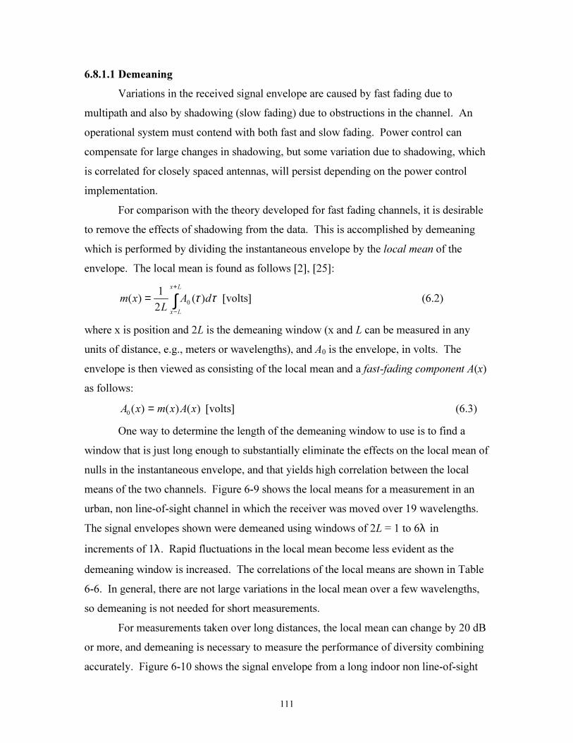
6.8.1.4 Diversity gain

Diversity gain was calculated as described in the Appendix. In Fig. 12, CDFs are

shown in Fig. 6-12 for the envelopes of the signals received by each diversity branch, as

well as for the calculated envelope of the signal after maximal ratio combining. This

particular experiment was performed in a non line-of-sight urban channel and used an

antenna spacing of d=0.5λ . The CDFs are normalized to the time average SNR of the

stronger branch. The diversity gain for a given cumulative probability (read from the y-

axis) is the horizontal distance between the curve for the stronger branch (channel 1 in

this case) and the curve for the combined signal. For example, the diversity gain from

Fig. 6-12 is approximately 6.7 dB for 10% cumulative probability and 11.6 dB for a 1%

cumulative probability. That is, diversity gain equals or exceeds 6.7 dB 10% of the time

and exceeds 11.6 dB 1% of the time.

Figure 6-11 . CDF of signal envelope with best fit Ricean CDF, K=1.5.

-35 -30 -25 -20 -15 -10 -5 0 5 1010

-3

10-2

10-1

100

Measured and best fit cdf

Envelope normalized to mean

Cum

ula

tive P

robability

envelope for branch 2

Best fit Ricean distribution, K = 1.5

Rayleigh distribution

117

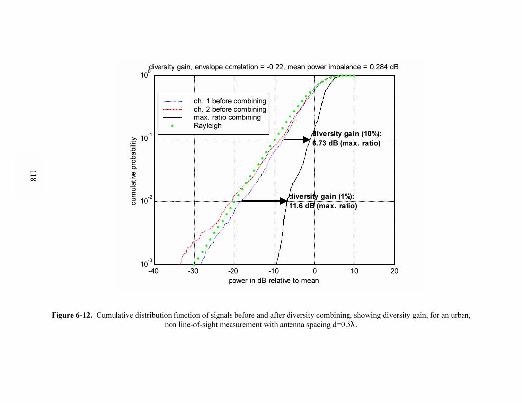
Figure 6-12. Cumulative distribution function of signals before and after diversity combining, showing diversity gain, for an urban,

non line-of-sight measurement with antenna spacing d=0.5λ .

-40 -30 -20 -10 0 10 2010

-3

10-2

10-1

100diversity gain, envelope correlation = -0.22, mean power imbalance = 0.284 dB

power in dB relative to mean

cum

ula

tive

pro

bability

diversity gain (10%):

6.73 dB (max. ratio)

diversity gain (1%):

11.6 dB (max. ratio)

ch. 1 before combiningch. 2 before combiningmax. ratio combiningRayleigh

118

119

6.8.2 Adaptive beamforming evaluation software

Each adaptive beamforming measurement is processed and then each set of

adaptive beamforming measurements is processed as shown in Fig. 6-13 (a) and (b),

respectively. Each individual measurement is processed in two steps as shown in Fig. 6-

13 (a). The raw data from each 4-channel adaptive beamforming measurement are stored

in two wave (.wav) files. The program “cmaproc4” reads the wave files and calculates

the signal to interference-plus-noise ratio (SINR), signal to noise ratio (SNR), and

synchronization error, and writes these data in a pre-processed (*.cma) file.

The program cmaproc4 uses several parameters that are specified by the user.

These include the block length used in the constant modulus algorithm, the block length

used to calculate SINR, the interval between orthogonalization of weights in the multi-

target algorithm, the number of algorithm iterations per block, the bandwidth to be used

in SINR and SNR calculations, and the name to be given to the pre-processed file. SINR

is calculated as follows. The FFT of the first second of data is calculated and the two

frequency bins that have the highest power are identified. For each data block of the

specified size, the SINR is calculated as the ratio of power in the bins in a specified

bandwidth about the frequency of the signal of interest to the power in the bins in the

same bandwidth about the frequency of the other signal. The SNR for each block is

calculated by dividing the power in the bins near the frequency of the signal of interest by

the power in an equivalent bandwidth about a baseband frequency of 7 kHz.

The program cmadisplay4 reads the data from the pre-processed (*.cma) data file,

and calculates and displays the mean SINR and SNR, and SINR and SNR for 10%, 1%,

and 0.1% cumulative probabilities. These data are stored in a structure called dabdata

and written to a processed data (*.dab) file. The program cmadisplay4 displays the SINR

and SNR vs. time, before and after combining, and the cumulative distribution functions

of the SINR and SNR. It also estimates the upper limit on possible SINR. This estimate

is equal to the sum of the mean SNRs on each of the receiver branches and represents the

mean SNR that would be achieved using maximal-ratio diversity combining in the

absence of interference.

Measurement sets, which consist of several measurement runs using different

antenna configurations and positioner angles, are processed based on information

120

contained in a measurement set description file with extension .abf. This file contains a

structure called abfdata that contains an output file name and directory and a list of

processed data files from individual measurements that are to be processed as part of the

set. The structure also contains information on the antenna spacing used for each

measurement, and descriptions of the antenna configuration, type of channel, location,

and date of the measurement set. The program “abfstats” reads the measurement set

description file and the processed data files for each measurement specified in the

measurement set description file, and calculates statistics for each measurement case used

in the measurement set. The calculated statistics are stored in a structure called pabdata

that also contains the information on the measurement set from the abfdata structure, and

the pab structure is written to a processed measurement set data file named *.pab. The

calculated statistics include the following for each measurement: the mean SINR and

SINR at cumulative probabilities of 10%, 1%, and 0.1% for each signal before and after

beamforming, and the synchronization error.

A sample plot of SINR vs. time is shown in Fig. 6-14 (a) and a plot of the CDF of

SINR is shown in Fig. 6-14 (b). In Fig. 6-14 (a) there are large variations in the SINR

before beamforming, due to multipath fading in both the desired and interfering signals.

The SINR after beamforming fluctuates rapidly but does not have large excursions. In

this measurement the mean SINR after beamforming is within about 2 dB of the

estimated value of 45.4 dB. Figure 6-14(b) shows the cumulative probability vs. SINR.

For example, for a cumulative probability of 10-2

or 1%, the SINR after beamforming,

shown by the solid line, is 31.4 dB. This is the SINR level that is exceeded 99% of the

time. By locating the dashed lines at the same cumulative probability level, it can be seen

that, at this cumulative probability level, the CMA algorithm has achieved an

improvement of 42 dB over the SINR measured on any of the four branches before

beamforming.

(a)

(b)

Figure 6-13. Data processing software modules for adaptive beamforming measurements:

(a) for individual measurement, (b) for measurement set.

cmaproc4 cmadisplay4

raw data

file

pre-processed

data file

processed data

file

Plots: SINR,

SNR vs. time,

and CDFs of

SINR, SNR

abfstats

processed data

file

Processed

meas. set data

file

Plots: SINR vs. Angle

or measurement case,

synchronization error

processed data

file

processed data

file...

measurement set

description

file

121

122

(a)

(b)

Figure 6-14. Plots of SINR from adaptive beamforming measurements: (a) SINR vs.

time, (b) cumulative probability of SINR.

0 5 10 15 20 25-40

-30

-20

-10

0

10

20

30

40

50

60Signal 2 before and after beamforming

Time, seconds

SIN

R,

dB

Ch. 1

Ch. 2

Ch. 3

Ch. 4

Output after CMA beamforming

Estimated mean output

-40 -30 -20 -10 0 10 20 30 40 50 6010

-4

10-3

10-2

10-1

100

Signal 2 before and after beamforming

SINR in dB

cum

ula

tive p

robabili

ty

Ch. 1

Ch. 2

Ch. 3

Ch. 4

Output after CMA beamforming

123

For measurement cases in which there is no interference, the least-squares constant

modulus algorithm (LSCMA), described in Chapter 3, provides diversity gain against

fading because it tends to maintain the envelope of the beamformer output at a nearly

constant level. To test the adaptive beamforming evaluation software, the diversity gain

achieved using LSCMA was compared to the calculated diversity gain for maximal ratio

combining. The adaptive beamforming software (cmaproc4 and cmadisplay4 shown in

Fig. 6-13) was used to process some of the data from measurements that had previously

been processed using the diversity combining evaluation software described in Section

6.8.1. The SNR after beamforming with the LSCMA was calculated and the diversity

gain using this algorithm was also calculated. Results for an urban, non line-of-sight

measurement are shown in Fig. 6-15.

Figure 6-15 (a) shows the results obtained for maximal ratio combining. It shows

cumulative probability as a function of SNR normalized to the mean SNR of the stronger

of the two branch signals, before processing. The cumulative probability distribution of

the calculated SNR for a maximal ratio combiner with a 500 Hz update rate is also

plotted. The horizontal difference between the two curves is the diversity gain in dB,

which is a function of the cumulative probability. The cumulative probability

distributions of the SNRs of the two branch signals and of the output signal after

processing with the LSCMA (with the weights updated 100 times per second) are shown

in Fig. 6-15 (b). The diversity gain achieved by the LSCMA beamformer is shown in Fig.

6-15 (b). As is expected, the agreement in diversity gains between the LSCMA and

maximal-ratio combining is very good. Maximal ratio combining provides diversity

gains of Gdiv,mr=6.7 dB at the 10% cumulative probability level and Gdiv,mr=11.6 dB at the

1% cumulative probability level. The diversity gains measured for the LSCMA

beamformer are Gdiv,LSCMA=6.3 dB at 10% cumulative probability and Gdiv,LSCMA=12.4 dB

at 1% cumulative probability. Agreement below the 1% level is not as close, probably

because the maximal ratio combining output SNR was calculated based on the input SNR

using a faster update rate than that used by the LSCMA beamformer.

124

-35 -30 -25 -20 -15 -10 -5 0 510

-3

10-2

10-1

100diversity gain, envelope correlation = -0.22, mean power imbalance = 0.282

SNR in dB relative to mean SNR of stronger branch

cum

ula

tive p

roba

bili

ty

ch. 1 before combining

ch. 2 before combining

max. ratio combining

Rayleigh

11.6 dB

6.7 dB

(a)

-10 -5 0 5 10 15 20 25 3010

-3

10-2

10-1

100

Signal 1 before and after beamforming

SNR in dB

cum

ula

tive p

roba

bili

ty

Ch. 1 before beamforming

Ch. 2 before beamforming

Output after CMA beamforming 6.3 dB

12.4 dB

(b)

Figure 6-15. Cumulative probability distributions showing diversity gain for: (a)

maximal ratio combining and (b) LSCMA beamformer.

6.9 Conclusions

This chapter described the Handheld Antenna Array Testbed (HAAT) and its

hardware and software components. The HAAT consists of a portable narrowband RF

measurement system that operates at 2.05 GHz and data processing hardware and

software. The HAAT allows quantitative evaluation of diversity combining and adaptive

125

beamforming using various array configurations and combining algorithms. The system

supports controlled measurements using a linear positioner to move the receiver and

measurements in which the receiver is carried by an operator as in typical handheld radio

operation. Two- and four-channel receiver and data logger units were constructed and

system link budgets were calculated based on the performance of each receiver. A single

transmitter is used in experiments that measure the effectiveness of diversity combining

to mitigate fading, and two transmitters are used in experiments that measure the

effectiveness of adaptive beamforming to reject interference. The data processing

software quantifies the performance of diversity combining or adaptive beamforming, to

facilitate comparison of different antenna configurations.