CHAPTER 6

TORSIONAL VIBRATIONS OF ROTORS-I:

THE DIRECT AND TRANSFER MATRIX METHODS

In previous chapters, mainly we studied transverse vibrations of simple rotor-bearing systems. It was

pointed out that transverse vibrations are very common in rotor systems due residual unbalances,

which is the most inherent fault in a rotor. We studied behaviour of rotor due to speed-independent

bearing dynamic parameters. Effect of gyroscopic couples on natural whirl frequencies is also

investigated in details. In the present chapter, we will extend the analysis of simple rotors to torsional

vibrations. We will start with the analysis of torsional vibrations of the single disc rotor, two disc

rotor, and three disc rotor systems with the conversional Newton’s second law of motion or energy

methods. The analysis is extended to the stepped shafts, geared systems, and branched systems. For

the multi-DOF system a general procedure of the transfer matrix method (TMM) is discussed for both

undamped and damped cases. Advantages and disadvantages of the TMM are outlined. In

reciprocating engines large variations of torque take place, however, periodically. This leads to

torsional resonances, and to analyse free and forced vibrations of these system a procedure is outline

to convert them to an equivalent multi-DOF rotor system, which is relatively easier to analyse. The

present chapter will pave the road for the TMM to be extended for the transverse vibrations of multi-

DOF rotor systems in subsequent chapters.

The study of torsional vibration of rotors is very important especially in applications where high

power transmission and high speed are present. Torsional vibrations are predominant whenever there

are large discs on relatively thin shafts (e.g., the flywheel of a punch press). Torsional vibrations may

original from the following forcings (i) inertia forces of reciprocating mechanisms (e.g., due to pistons

in IC engines), (ii) impulsive loads occurring during a normal machine cycle (e.g., during operations

of a punch press), (iii) shock loads applied to electrical machinery (such as a generator line fault

followed by fault removal and automatic closure), (iv) torques related to gear mesh frequencies, the

turbine blade and compressor fan passing frequencies, etc.; and (v) a rotor rubs with the stator. For

machines having massive rotors and flexible shafts (where system natural frequencies of torsional

vibrations may be close to, or within, the source frequency range during normal operation) torsional

vibrations constitute a potential design problem area. In such cases designers should ensure the

accurate prediction of machine torsional frequencies, and frequencies of any torsional load

fluctuations should not coincide with torsional natural frequencies. Hence, determination of torsional

natural frequencies of the rotor system is very important and in the present chapter we shall deal with

it in great detail.

272

6.1 A Simple Rotor System with a Single Disc Mass

Consider a rotor system as shown Figure 6.1(a). The shaft is considered as mass-less and it provides

torsional stiffness. The disc is considered as rigid and has no flexibility. If an initial disturbance is

given to the disc in the torsional mode (about its longitudinal or polar axis) and allow it to oscillate its

own, it will execute free vibrations. Figure 6.2 shows that rotor is spinning with a nominal speed of ω

and executing torsional vibrations, ϕz(t), due to this it has actual speed of ( )z

tω ϕ+ � . It should be noted

that the spinning speed, ω, remains the same, however, the angular velocity due to torsion have

varying direction over a period. In actual practice if we tune a stroboscope (it is a speed/frequency

measuring instrument, refer Chapter 15) flashing frequency to the nominal speed of a rotor then free

torsional oscillations could be observed. For the present case and in most of our analysis, it is assumed

that torsional natural frequency does not depend upon the spin speed of rotor. Hence, in limiting case

when the spin speed is zero the natural frequency of the non-spinning rotor will be same as at any

other speed. The free oscillation will be simple harmonic motion with a unique frequency, which is

called the torsional natural frequency of the rotor system.

Figure 6.1(a) A single-mass cantilever rotor system (b) A free body diagram of the disc

Figure 6.2 Torsional vibrations of a spinning rotor

273

From the theory of torsion of the shaft (Timoshenko and Young, 1968), we have

t

z

T GJk

lϕ= = with

4

32J d

π= (6.1)

where kt is the torsional stiffness of shaft, Ip is the polar mass moment of inertia of the disc, J is the

polar second moment of area of the shaft cross-section, l is the length of the shaft, d is the diameter of

the shaft, and zϕ is the angular displacement of the disc (the counter clockwise direction is assumed

as the positive direction). From the free body diagram of the disc as shown in Figure 6.1(b), we have

External torque of disc z t z zp pkI Iϕ ϕ ϕ− == ⇒∑ �� �� (6.2)

where ∑ represents the summation operator. Equation (6.2) is the equation of motion of the disc for

free torsional vibrations. The free (or natural) vibration has a simple harmonic motion (SHM). For

SHM of the disc, we have

( ) sinz z nf

t ω tϕ = Φ so that 2 2sinz nf z nf nf zω ω t ωϕ ϕ= − Φ = −�� (6.3)

where z

Φ is the amplitude of the torsional vibration, and nf

ω is the torsional natural frequency. On

substituting equation (6.3) into equation (6.2), we get

( )2

t z p nf zk Iϕ ω ϕ− = − or ( )2 0

z nf p tI kϕ ω − = (6.4)

Since 0z

ϕ ≠ , it gives

tnf

p p

k GJ

I lIω = = (6.5)

which is similar to the case of single-DOF spring-mass system in where the polar mass moment of

inertia and the torsional stiffness replace the mass and the spring stiffness, respectively.

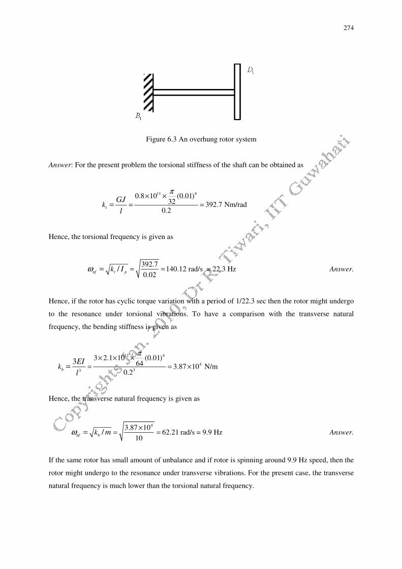
Example 6.1 Obtain the torsional natural frequency of an overhung rotor system as shown in Fig. 6.3.

The end B1 of the shaft has fixed end conditions. The shaft diameter is 10 mm and the length of the

span is 0.2 m. The disc D1 is thin, and has mass of 10 kg and the polar mass moment of inertia equal

to 0.02 kg-m2. Neglect the mass of the shaft.

274

Figure 6.3 An overhung rotor system

Answer: For the present problem the torsional stiffness of the shaft can be obtained as

11 40.8 10 (0.01)32 392.7 Nm/rad

0.2tk

GJ

l

π× ×

= ==

Hence, the torsional frequency is given as

392.7140.12 rad/s

0.02/

nf t pk Iω = == = 22.3 Hz Answer.

Hence, if the rotor has cyclic torque variation with a period of 1/22.3 sec then the rotor might undergo

to the resonance under torsional vibrations. To have a comparison with the transverse natural

frequency, the bending stiffness is given as

11 4

4

33

3 2.1 10 (0.01)64 3.87 10 N/m

0.2

3b

kEI

l

π× × ×

= = ×=

Hence, the transverse natural frequency is given as

43.87 10

62.21 rad/s10

/nf b

k mω×

= == = 9.9 Hz Answer.

If the same rotor has small amount of unbalance and if rotor is spinning around 9.9 Hz speed, then the

rotor might undergo to the resonance under transverse vibrations. For the present case, the transverse

natural frequency is much lower than the torsional natural frequency.

275

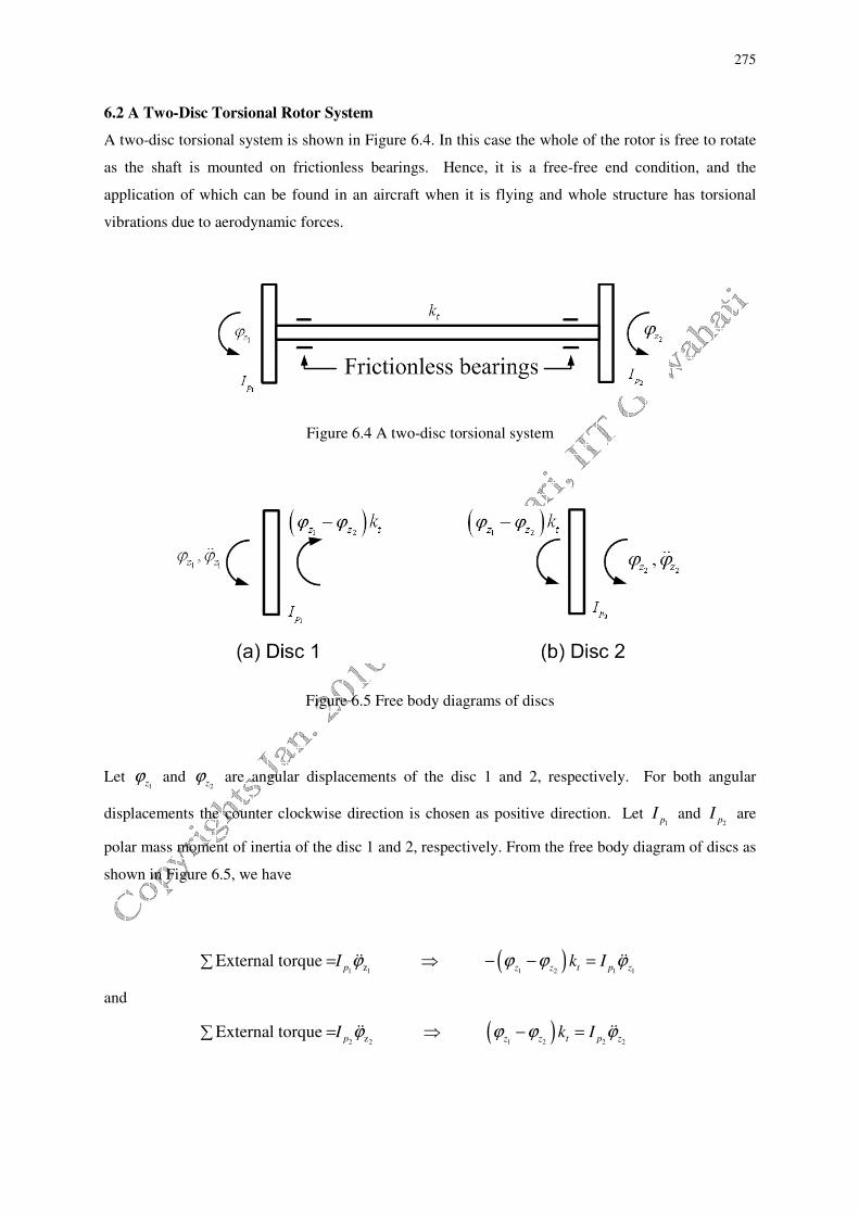
6.2 A Two-Disc Torsional Rotor System

A two-disc torsional system is shown in Figure 6.4. In this case the whole of the rotor is free to rotate

as the shaft is mounted on frictionless bearings. Hence, it is a free-free end condition, and the

application of which can be found in an aircraft when it is flying and whole structure has torsional

vibrations due to aerodynamic forces.

Figure 6.4 A two-disc torsional system

Figure 6.5 Free body diagrams of discs

Let 1z

ϕ and 2z

ϕ are angular displacements of the disc 1 and 2, respectively. For both angular

displacements the counter clockwise direction is chosen as positive direction. Let 1p

I and 2p

I are

polar mass moment of inertia of the disc 1 and 2, respectively. From the free body diagram of discs as

shown in Figure 6.5, we have

( )1 1 1 2 1 1zExternal torque

p z z t p zI k Iϕ ϕ ϕ ϕ= ⇒ − − =∑ �� ��

and

( )2 2 1 2 2 2zExternal torque

p z z t p zI k Iϕ ϕ ϕ ϕ= ⇒ − =∑ �� ��

276

where kt is the torsional stiffness of the shaft, and let ( )1 2z z

ϕ ϕ− be the relative twist of the shaft ends.

Above expressions give the following equations of motion

1 1 2 2 2 12

0 and 0p z t z t z p z t z t z

I k k I k kϕ ϕ ϕ ϕ ϕ ϕ+ − = + − =�� �� (6.6)

For free vibrations, we have SHM, so the solution will take the form

1 1

2

z nf zωϕ ϕ= −�� and 2 1

2

z nf zωϕ ϕ= −�� (6.7)

Substituting equation (6.7) into equation (6.6), it gives

1 1 21

2 0p z t z t z

I k kω ϕ ϕ ϕ− + − = and 2 2 12

2 0p nf z t z t z

I k kω ϕ ϕ ϕ− + − = (6.8)

Noting equation (6.3), equation (6.8) can be assembled in a matrix form as

[ ]{ } { }0zD Φ = (6.9)

with

[ ] 1

2

2

2

t p nf t

t t p nf

k I kD

k k I

ω

ω

− −=

− − ; { } 1

2

z

z

z

Φ Φ =

Φ

The non-trial solution of equation (6.9) is obtained by taking determinant of the matrix [D] equal to

zero, as

0D =

which gives

( )( )1 2

2 2 2 0t p n t p n t

k I k I kω ω− − − = or ( )1 21 2

4 2 0p p nf p p t nf

I I I I kω ω− + = (6.10)

Roots of equation (6.10) are given as

( )

1 2

1 2

1 2

0 andp p t

nf nf

p p

I I k

I Iω ω

+= = (6.11)

Hence, the system has two torsional natural frequencies and one of them is zero. From equation (6.9)

corresponding to first natural frequency for 1nf

ω = 0, we get

277

z zΦ = Φ

1 2 (6.12)

Figure 6.6 The first mode shape

From equation (6.12), it can be concluded that, the first root of equation (6.10) represents the case

when both discs simply rolls together in phase with each other as shown in Figure 6.6. The

representation of the relative angular displacement of two discs in this form is called the mode shape.

The mode shape shown in Fig. 6.6 is called the rigid body mode, which is of a little practical

significance because no stresses develop in the shaft. This mode it generally occurs whenever the

system has free-free boundary conditions (for example an aeroplane during flying).

Figure 6.7 (a) The second mode (b) equivalent system 1 (c) equivalent system 2

278

Now from first set of equation (6.9), for 2nf nf

ω ω= , we get

( )1 2 1 2

2 0t p nf z t z

k I kω− Φ − Φ = or

1 2

1 1 2

1 2

0p p

t p t z t z

p p

I Ik I k k

I I

+− Φ − Φ =

which gives relative amplitudes of two discs as

1 2

2 1

z p

z p

I

I

Φ= −

Φ (6.13)

The second mode shape from equation (6.13) represents the case when both masses oscillate in anti-

phase with one another (i.e., the direction of rotation of one disc will also be opposite to the other).

Both discs will reach their extreme angular positions simultaneously, and both will reach the static

equilibrium (untwisted) position also simultaneously. It should be noted that both the discs have same

frequency of oscillation (i.e., the time period) but different angular amplitude. Figure 6.7 shows this

mode shape of the two-rotor system. From two similar triangles in Figure 6.7(a), we have

1 2 1

2

1

1 2 2

z z z

z

l

l l l

Φ Φ Φ= ⇒ =

Φ (6.14)

where l1 and l2 are node position from discs 1 and 2, respectively (Fig. 6.7a). Since both the masses

are always vibrating in the opposite direction, there must be a point on the shaft where torsional

vibration is not taking place, i.e. where the angular displacement is zero. This point is called a node.

The location of the node may be established by treating each end of the real system as a separate

single-disc cantilever system as shown in Figure 6.7(a). The node is treated as the point, where the

shaft is rigidly fixed. Hence, basically we will have two single-DOF overhung rotor systems (Fig.

6.7b) instead of one two-DOF free-free rotor system (Fig. 6.7c). Since value of natural frequency is

known (the frequency of oscillation of each of the single-disc overhung system must be same), hence

we write

1 2

2

1 2

2 t t

nf

p p

k k

I Iω = = (6.15)

where 2nfω is defined by equation (6.11),

1tk and

2tk are the torsional stiffness of two single-DOF

overhung rotor systems, which can be obtained from equation (6.15), as

279

1 2 1 2 2 2

2 2 and t nf p t nf pk I k Iω ω= =

Lengths l1 and l2 then can be obtained as

1 1

1 2andt t

GJ GJl l

k k= = with 1 2l l l+ = (6.16)

which will give the node position. It should be noted that the shear stress would be maximum at the

node point being a fixed end of overhung rotor systems.

Example 6.2 Determine natural frequencies and mode shapes for a rotor system as shown in Figure

6.8. Neglect the mass of the shaft and assume that discs as lumped masses. The shaft is 1 m of length,

0.015m of diameter, and 0.8×1011

N/m of modulus of rigidity. Discs have polar mass moment of

inertia as 1

0.01pI = kg-m2 and

20.015pI = kg-m

2.

Figure 6.8 A two-disc rotor system

Solution: The stiffness of the shaft can be obtained as

11 40.8 10 (0.015) / 32

397.61 Nm/rad1.0

tkGJ

l

π× ×= ==

The natural frequency is given as

( )

1 2

0.01 0.015 397.61

0.01 0.0150 and

nf nfω ω

+ ×

×= = = 257.43 rad/s

The relative displacements would be

280

1 2

2 1

0.0151.5

0.01

z p

z p

I

I

Φ= − = − = −

Φ

which means disc 1 would have 1.5 times angular displacement amplitude as compared to the disc 2,

however, in opposite direction. The node position can be obtained as

2

1

1

2

0.0151.5

0.01

p

p

Il

l I= = = ; and 1 2 1l l+ =

Hence, we get the node location as 1 0.6l = m (i.e., 0.6 m from disc 1 refer to Fig. 6.7(a)). It can be

verified that equivalent two single-mass cantilever rotors will have the same natural frequency, as

1

11 4

1

0.8 10 (0.015) / 32662.68 Nm/rad

0.6tk

GJ

l

π× ×= ==

and

2

11 4

2

0.8 10 (0.015) / 32994.03 Nm/rad

0.4tk

GJ

l

π× ×= ==

so that

1

2

1

(1) 662.68257.43

0.01

t

nf

p

k

Iω = = = rad/s

and

2

2

2

(2) 994.03257.43

0.015

t

nf

p

k

Iω = = = rad/s Answer

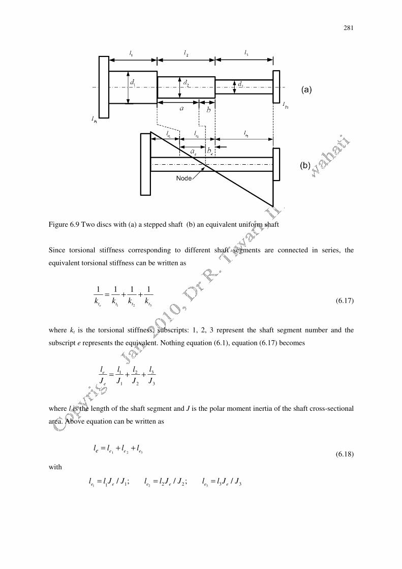
6.3 A Two-Disc Rotor System with a Stepped Shaft

Figure 6.9(a) shows a stepped shaft with two large discs at ends with Ip (subscript 1 and 2 represent

left and right side disc, respectively) is the polar mass moment of inertia. It is assumed that the rotor

has free-free boundary conditions and the polar mass moment of inertia of shaft is negligible as

compared to two discs at either ends of the shaft. In such cases the actual shaft should be replaced by

an unstepped equivalent shaft for the purpose of the analysis as shown in Fig. 6.9(b). The equivalent

shaft diameter may be same as the smallest diameter of the real shaft (or any other diameter). The

equivalent shaft must have the same torsional stiffness as the real shaft.

281

Figure 6.9 Two discs with (a) a stepped shaft (b) an equivalent uniform shaft

Since torsional stiffness corresponding to different shaft segments are connected in series, the

equivalent torsional stiffness can be written as

1 2 3

1 1 1 1

et t t tk k k k

= + + (6.17)

where kt is the torsional stiffness, subscripts: 1, 2, 3 represent the shaft segment number and the

subscript e represents the equivalent. Nothing equation (6.1), equation (6.17) becomes

31 2

1 2 3

e

e

l ll l

J J J J= + +

where l is the length of the shaft segment and J is the polar moment inertia of the shaft cross-sectional

area. Above equation can be written as

1 2 3e e eel l l l= + + (6.18)

with

1 2 31 2 2 3 31/ ; / ; /

e e e e e el l J J l l J J l l J J= = =

282

where 1 2 3, ,e e el l l are equivalent lengths of shaft segments having the equivalent shaft diameter d3, and le

is the total equivalent length of the unstepped shaft as shown in Figure 6.9(b). Let us assume that the

node position in the equivalent shaft system comes out in the second shaft segment from the previous

section analysis. Noting equations (6.15) and (6.16), the node location in the equivalent shaft from

Figure 6.9(b) can be obtained as

1

2 1

2

ee e

nf p

GJl a

Iω+ =

and 3

2 2

2

ee e

nf p

GJl b

Iω+ =

(6.19)

with

( )( ) ( ) ( )

1 2

2

1 2

1 1 2 2 3 3

1and

ep p t

nf te

p p

I I kk

I I l GJ l GJ l GJω

+=

= + +

From equation (6.19), the node position (i.e., ae or be in Fig. 6.9(b)) can be obtained, the

corresponding node location in the real shaft system can be obtained as explained below. From

equation (6.18), we have

4 4 4

2 3 2 22

2

; ; 32 32 32

ee e e

Jl l J d d J d

J

π π π= = = = (6.20)

Since equation (6.20) is for the shaft segment in which node is assumed to be present, we can write

2 2

and e ee e

J Ja a b b

J J= = (6.21)

where a and b are node position in real system (Fig.6.9(a)). Equation (6.21) can be combined as

e

e

aa

b b= (6.22)

So once ae or be is obtained from equation (6.19), the location of the node in the actual shaft can be

obtained from equation (6.22). The final location of the node on the shaft in the real system is given in

the same proportion as in the shaft of equivalent system in which the node occurs.

Example 6.3 Consider a stepped shaft with two discs as shown in Fig. 6.10. The following shaft

dimensions are to be taken: l1 = 0.5m, l2 = 0.3m, l3 = 0.2m, d1 = 0.015m, d2 = 0.012m, d3 = 0.01m.

Take the modulus of rigidity of the shaft as 0.8×1011

N/m. Discs have polar mass moment of inertia as

283

1pI = 0.015 kg-m2 and

20.01pI = kg-m

2. Obtain natural frequencies, mode shapes, and the location of

the node.

Fig. 6.10 A stepped shaft with two discs

Solution: Let us represent shaft segments towards the left, middle and right sides as 1, 2 and 3,

respectively. For the present problem the shaft has following data

4 49 41

1

0.0154.97 10 m

32 32

dJ

π π −× ×= = ×= ; 9 4

2 2.036 10 mJ−×= ; 9 4

3 0.982 10 mJ−×= ;

1

11 9

1

1

0.8 10 4.97 10795.20 Nm/rad

0.5tk

GJ

l

−× × ×= == ;

2542.93 Nm/radtk = ;

3392.80 Nm/radtk =

For the stepped shaft the first step would be to obtain the equivalent length with respect to a reference

shaft 3 that has diameter of 0.01 m, as

31 2

1 2 3

0.5 0.3 0.20.982 0.982 0.982 0.0988 0.1447 0.2 0.4435m

4.97 2.036 0.982e e e e

ll ll J J J

J J J= = + + == + + + +

Hence, The equivalent stiffness can be calculated as

11 90.8 10 0.982 10177.14 Nm/rad

0.4435e

e

e

tkGJ

l

−× × ×= ==

Hence, 1

0.0987el = m and 2

0.1447el = m. The natural frequency of the rotor system can be calculated

as

( ) ( )1 2

2

1 2

=

0.015 0.01 177.14

0.015 0.01

ep p t

nf

p p

I I k

I Iω

+ + ×

×==171.82 rad/sec

284

Relative displacements of the rotor system would be

1 2

2 1

0.010.667

0.015

z p

z p

I

I

Φ= − = −

Φ= −

which means disc 1 would have 0.0667 times angular displacement amplitude as compared to the disc

2, however, in opposite direction. It is interesting that relative displacement remains same irrespective

of shaft characteristics (i.e., stepped, uniform, etc.) and its stiffness. However, the node position

depends upon the shaft characteristics and its stiffness, and can be obtained as for equivalent shaft as

1 2

2 1

0.010.667

0.015

ne p

ne p

l I

l I= == ; and

1 20.4435ne ne el l l+ = = m

Hence, we get the node location as 2

0.266nel = m (i.e., 0.266 m from disc 2 in the equivalent system

see Fig. 6.11). Hence, we have 1

0.1775nel = m. This means the node will be in second (middle) shaft

segment. The location in actual rotor system would be

1 1

2 3

0.1775 0.0988 0.07871.1924

0.266 0.2 0.066

ne ee

e ne e

l laa

b b l l

− −= = = = =

− −; and 0.1447a b+ = m

Hence, we have the position of the node in actual system as: b = 0.137m and a = 0.163m (see Fig.

6.9).

Fig. 6.11 (a) Equivalent system and (b) its mode shape and node position

285

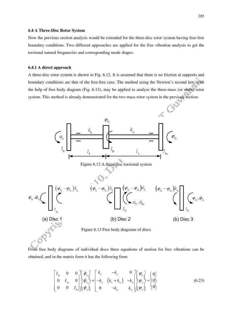
6.4 A Three-Disc Rotor System

Now the previous section analysis would be extended for the three-disc rotor system having free-free

boundary conditions. Two different approaches are applied for the free vibration analysis to get the

torsional natural frequnecies and corresponding mode shapes.

6.4.1 A direct approach

A three-disc rotor system is shown in Fig. 6.12. It is assumed that there is no friction at supports and

boundary conditions are that of the free-free case. The method using the Newton’s second law, with

the help of free body diagram (Fig. 6.13), may be applied to analyse the three-mass (or more) rotor

system. This method is already demonstrated for the two-mass rotor system in the previous section.

Figure 6.12 A three-disc torsional system

Figure 6.13 Free body diagrams of discs

From free body diagrams of individual discs three equations of motion for free vibrations can be

obtained, and in the matrix form it has the following form

( )1 1

1 1 1

2 2 1 1 2 2 2

3 3 32 2

00 0 0

0 0 0

00 0 0

t tp z z

p z t t t t z

p z zt t

k kI

I k k k k

I k k

ϕ ϕ

ϕ ϕ

ϕ ϕ

−

+ − + − =

−

��

��

��

(6.23)

286

For free vibrations, which has the SHM, it takes the form

( )1 1

1 1

2 1 1 2 2 2

3 32 2

2

00 0 0

0 0 0

00 0 0

t tp z

nf p t t t t z

p zt t

k kI

I k k k k

I k k

ϕ

ω ϕ

ϕ

− − + − + − = −

(6.24)

where nfω is the torsional natural frequency of the rotor system. For finding natural frequencies two

methods can be adopted (i) by obtaining characteristic (or frequency) equations, and (ii) by

formulating an eigen value problem.

Characteristic (or frequency) equations:

On equating the determinant to zero of the matrix in equation (6.24), we get the characteristic

equation of the following form

( )1 2 1 2 32 31 2

1 2

1 2 2 3 1 2 3

2 4 2 0t t p p pp pp p

nf nf t t nf

p p p p p p p

k k I I II II Ik k

I I I I I I Iω ω ω

+ + ++ − + + =

which gives natural frequencies as

1

0nfω = ;

and

( )1 2 1 2 32 3 2 31 2 1 2

2,3 1 2 1 2

1 2 2 3 1 2 2 3 1 2 3

2

2 1 1

2 4

t t p p pp p p pp p p p

nf t t t t

p p p p p p p p p p p

k k I I II I I II I I Ik k k k

I I I I I I I I I I Iω

+ + + ++ + = + ± + −

(6.25)

Mode shapes can be obtained by substituting natural frequencies obtained, one by one, into the

equations (6.24) and obtaining relative amplitudes with the help of any two equations (out of three

equations), as

( )1 1 1 1 2

2 0t nf p z t z

k I kω ϕ ϕ− − = ( )

1 12

1 1

2

t nf pz

z t

k I

k

ωϕ

ϕ

−⇒ = (6.26)

and

( ){ }1 1 1 2 2 2 2 3

2 0t z t t nf p z t zk k k I kϕ ω ϕ ϕ− + + − − = (6.27)

287

On substituting equation (6.26) in equation (6.27), we get

( ){ } ( ){ }1 1 1 2 2 1 1 1 1 2 3

2 2 / 0t z t t nf p t nf p z t t zk k k I k I k kϕ ω ω ϕ ϕ− + + − − − = (6.28)

which can be simplified to

( ) ( ){ } ( )

1 2 1 2 1 1 2 1 23

1 1 2

4 2

p p nf p p t p t nf t tz

z t t

I I I I k I k k k

k k

ω ωϕ

ϕ

− + + += (6.29)

It should be noted that from equations (6.26) and (6.29) for 1

0nfω = , we have 2 1 3 1

/ / 1z z z zϕ ϕ ϕ ϕ= =

(or 1 2 3z z zϕ ϕ ϕ= = ) that belongs to the rigid body mode. Similarly, for the other two natural

frequencies relative amplitudes of disc can be obtained by substituting these natural frequencies one

by one in equations (6.26) and (6.29).

An eigen value problem:

A more general method of obtaining of natural frequencies and mode shapes is to formulate an eigen

value problem and that can relatively easily be solved by computer routines. Eigen values of the eigen

value problem of equation (6.24) gives natural frequencies, and eigen vectors represent mode shapes.

Equation (6.24) can be written as

[ ] [ ]( ){ } { }2 0nf

M Kω− + Φ = (6.30)

with

1

2

3

0 0

[ ] 0 0

0 0

p

p

p

I

M I

I

=

; ( )1 1

1 1 2 2

2 2

0

[ ]

0

t t

t t t t

t t

k k

K k k k k

k k

−

= − + −

−

; { }1

2

3

z

z

z

ϕ

ϕ

ϕ

Φ =

On multiplying both sides by the inverse of mass matrix in equation (6.30), we get a standard eigen

value problem of the following form

[ ] [ ]( ){ } { }2 0nf

I Dω− + Φ = (6.31)

with

1[ ] [ ] [ ]D M K−=

288

The eigen value and eigen vector of the matrix [D] can be obtained conveniently by hand calculations

for the matrix size up to 3×3, however, for the larger size matrix from multi-DOF rotor systems any

standard software (e.g., MATLAB) could be used. The square root of eigen values will give the

natural frequencies and corresponding eigen vectors as mode shapes (i.e., relative amplitudes). These

methods would now be illustrated through an example.

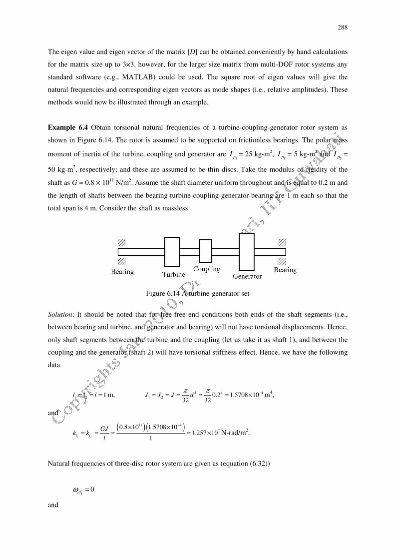
Example 6.4 Obtain torsional natural frequencies of a turbine-coupling-generator rotor system as

shown in Figure 6.14. The rotor is assumed to be supported on frictionless bearings. The polar mass

moment of inertia of the turbine, coupling and generator are p

I1= 25 kg-m

2,

pI

2= 5 kg-m

2 and

pI

3=

50 kg-m2, respectively; and these are assumed to be thin discs. Take the modulus of rigidity of the

shaft as G = 0.8 × 1011

N/m2. Assume the shaft diameter uniform throughout and is equal to 0.2 m and

the length of shafts between the bearing-turbine-coupling-generator-bearing are 1 m each so that the

total span is 4 m. Consider the shaft as massless.

Figure 6.14 A turbine-generator set

Solution: It should be noted that for free-free end conditions both ends of the shaft segments (i.e.,

between bearing and turbine, and generator and bearing) will not have torsional displacements. Hence,

only shaft segments between the turbine and the coupling (let us take it as shaft 1), and between the

coupling and the generator (shaft 2) will have torsional stiffness effect. Hence, we have the following

data

1 2

1l l l= = = m, 4 4 4

1 20.2 1.5708 10

32 32J J J d

π π −= = = = = × m4,

and

( ) ( )

1 2

11 4

70.8 10 1.5708 10

1.257 101

t t

GJk k

l

−× ×= = = = × N-rad/m

2.

Natural frequencies of three-disc rotor system are given as (equation (6.32))

10nfω =

and

289

( )1 2 1 2 32 3 2 31 2 1 2

2,3 1 2 1 2

1 2 2 3 1 2 2 3 1 2 3

2

2 1 1

2 4

t t p p pp p p pp p p p

nf t t t t

p p p p p p p p p p p

k k I I II I I II I I Ik k k k

I I I I I I I I I I Iω

+ + + ++ + = + ± + −

On substituting values of various parameters of the present problem in above equation, it gives

20nfω = rad/s;

2611.56nfω = rad/s;

32325.55nfω = rad/s;

The mode shape (relative angular displacements of various discs) can be obtained as summarised in

Table 6.1 (refer equations (6.33) and (6.34)). Fig. 6.15 shows mode shapes with node locations, in

drawing T, C and G represent location of the turbine, coupling and generator, respectively.

Table 6.1 Relative angular displacements of various discs

Relative displacement 2

0nfω = rad/s 2

611.56nfω = rad/s 3

2325.55nfω = rad/s

2 1 1

1 1

2

z t nf p

z t

k I

k

ϕ ω

ϕ

−=

1

0.2563

-9.7600

( ) ( ){ } ( )1 2 1 2 1 1 2 1 23

1 1 2

4 2

p p nf p p t p t nf t tz

z t t

I I I I k I k k k

k k

ω ωϕ

ϕ

− + + +=

1

-0.5256

0.4754

Fig. 6.15 Three mode shapes corresponding to three torsional natural frequencies

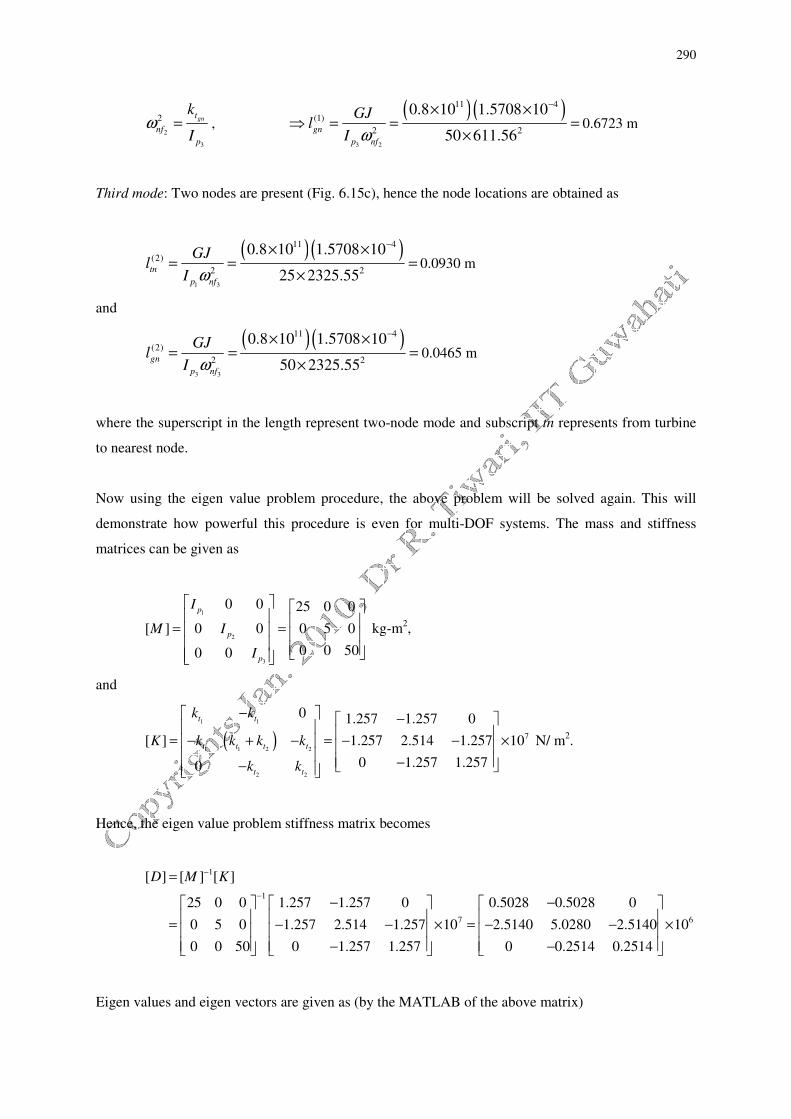
Node locations in the second and third modes can be obtained as follows:

Second mode: Only single node (Fig. 6.15b) is present between the coupling and the generator. Hence,

from the node position to the generator a single-DOF rotor system can be assumed with the length of

shaft as (1)

gnl (superscript corresponding to single-node mode and subscript gn represent from

generator to node) and polar mass moment of inertia as 3p

I , this gives

290

2

3

2 gnt

nf

p

k

Iω = ,

( ) ( )3 2

11 4

(1)

2 2

0.8 10 1.5708 10

50 611.56gn

p nf

GJl

I ω

−× ×⇒ = = =

×0.6723 m

Third mode: Two nodes are present (Fig. 6.15c), hence the node locations are obtained as

( )( )1 3

11 4

(2)

2 2

0.8 10 1.5708 10

25 2325.55tn

p nf

GJl

I ω

−× ×= = =

×0.0930 m

and

( )( )3 3

11 4

(2)

2 2

0.8 10 1.5708 10

50 2325.55gn

p nf

GJl

I ω

−× ×= = =

×0.0465 m

where the superscript in the length represent two-node mode and subscript tn represents from turbine

to nearest node.

Now using the eigen value problem procedure, the above problem will be solved again. This will

demonstrate how powerful this procedure is even for multi-DOF systems. The mass and stiffness

matrices can be given as

1

2

3

0 0 25 0 0

[ ] 0 0 0 5 0

0 0 500 0

p

p

p

I

M I

I

= =

kg-m2,

and

( )1 1

1 1 2 2

2 2

7

0 1.257 1.257 0

[ ] 1.257 2.514 1.257 10

0 1.257 1.2570

t t

t t t t

t t

k k

K k k k k

k k

− − = − + − = − − × −−

N/ m2.

Hence, the eigen value problem stiffness matrix becomes

1

1

7 6

[ ] [ ] [ ]

25 0 0 1.257 1.257 0 0.5028 0.5028 0

0 5 0 1.257 2.514 1.257 10 2.5140 5.0280 2.5140 10

0 0 50 0 1.257 1.257 0 0.2514 0.2514

D M K−

−

=

− − = − − × = − − × − −

Eigen values and eigen vectors are given as (by the MATLAB of the above matrix)

291

{ }.

.λ

= ×

6

5 4082

0 3740 10

0

, and [ ]. . .

. . .

. . .

X

− − = − −

0 1018 0 8632 0 5774

0 9936 0 2212 0 5774

0 0484 0 4537 0 5774

Where the columns of matrix [X] represent the mode shapes. Hence, natural frequencies are obtained

as

{ } { }.

.

nf

nf nf

nf

ω

ω ω λ

ω

= = =

3

2

1

2325 55

611 56

0

rad/s

The mode shape can be normalised as (in each column elements is divided by the corresponding first

row element, e.g. 0.9936/(-0.018) = -9.76), -0.0484/(-0.018) = 0.48, -0.2212/(-0.8632) = 0.26, etc.)

[ ] . .

. .

T T T

C C C

G G Gnf nf nf

x x x

x x x

x x x

X

ω ω ω

ϕ ϕ ϕ

ϕ ϕ ϕ

ϕ ϕ ϕ

= = − − 13 2

1 1 1

9 76 0 26 1

0 48 0 53 1

These mode shapes are exactly same as in Fig. 6.15.

6.4.2 An indirect approach

From the previous method, it is clear that for a particular natural frequency a unique mode shape

exists. In the present method, the information regarding the possible mode shapes would be utilised to

get the corresponding natural frequencies. In case the shaft has steps then, the first step would be to

reduce the actual shaft to an equivalent shaft of uniform diameter as shown in Figure 6.16(a).

For three-disc rotor system, three natural frequencies are expected and correspondingly three natural

(or normal) modes of vibrations. Since the free-free boundary conditions one of the modes would be

the rigid-body mode, in which all the discs have same motion. Apart from the rigid body mode, there

will be two possible natural modes of vibration, in which the rotors all reach their extreme positions at

same instant and all pass through their equilibrium position at the same instant. There will be a

different natural frequency for each of these normal modes.

In one mode there is a single node (a point where there will not be any angular displacement) between

discs 1 and 2 or between discs 2 and 3 (see Figure 6.16(b)). It depends upon the relative polar mass

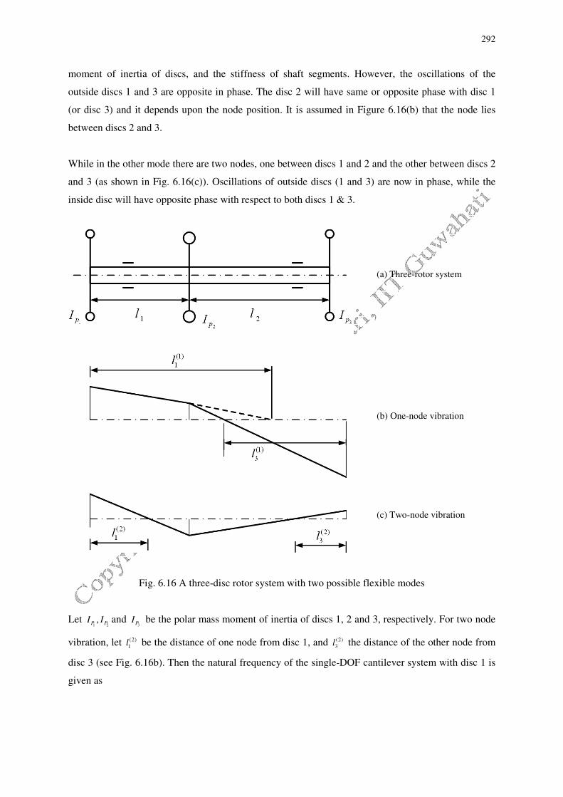
292

moment of inertia of discs, and the stiffness of shaft segments. However, the oscillations of the

outside discs 1 and 3 are opposite in phase. The disc 2 will have same or opposite phase with disc 1

(or disc 3) and it depends upon the node position. It is assumed in Figure 6.16(b) that the node lies

between discs 2 and 3.

While in the other mode there are two nodes, one between discs 1 and 2 and the other between discs 2

and 3 (as shown in Fig. 6.16(c)). Oscillations of outside discs (1 and 3) are now in phase, while the

inside disc will have opposite phase with respect to both discs 1 & 3.

Fig. 6.16 A three-disc rotor system with two possible flexible modes

Let 1 2,P PI I and

3PI be the polar mass moment of inertia of discs 1, 2 and 3, respectively. For two node

vibration, let (2)

1l be the distance of one node from disc 1, and (2)

3l the distance of the other node from

disc 3 (see Fig. 6.16b). Then the natural frequency of the single-DOF cantilever system with disc 1 is

given as

(a) Three-rotor system

(b) One-node vibration

(c) Two-node vibration

293

1

1

1 1

(2)

(2)

(2)

1

1t

nf

p p

k GJ

I Ilω = = (6.35)

Similarly, for the single-DOF cantilever system with disc 3 (Figure 6.16c), we have

3

3

(2)

(2)

3

1nf

p

GJ

Ilω = (6.36)

For the single-DOF fixed-fixed system with disc 2 (Fig. 6.16c), we have

2

2

2

(2)

(2) t

nf

p

k

Iω = (6.37)

where

( )( )2

(2) (2)

(2) 1 2 1 3

(2) (2) (2) (2)1 1 2 3 1 1 2 3

t

l l l lGJ GJk GJ

l l l l l l l l

+ − −= + =

− − − − (6.38)

where bt

k is the torsional stiffness of a rotor system with fixed-fixed end conditions. On substituting

equation (6.38) into equation (6.37), we get

( )( )( )2

2

(2) (2)

1 2 1 3(2)

(2) (2)

1 1 2 3

nf

p

l l l lGJ

I l l l lω

+ − −=

− − (6.39)

Since for a particular mode all frequencies 1 2

(2) (2), nf nfω ω and

3

(2)

nfω must be equal (superscript represents

the two-node mode). This leads to two independent equations to be solved for (2)

1l and (2)

3l . Once we

know these node positions we could be able to get the natural frequency of the two-node (or one-

node) mode. On equating equations (6.35) and (6.36), we get

1 3

(2) (2)

1 3p pl I l I= (6.40)

Similarly on equating equations (6.35) and (6.39), we get

( )( )( )

21

(2) (2)

1 2 1 3

(2) (2) (2)1 1 1 2 3

1 1

pp

l l l l

Il I l l l l

+ − −=

− − (6.41)

294

Equation (6.40) can be used to eliminate (2)

1l from equation (6.41), and it get simplified to

( ) ( )2 3 3 3 2

3 2 3 2

1 1 1

22 2(2) (2)

3 1 1 2 3 1 20

p p p p p

p p p p

p p p

I I I I I lI l I l I l l l I l l

I I I

+ + − + + + + =

(6.42)

The two roots of (2)

3l from this quadratic give positions of nodes for the one-node and two-node

vibration frequencies. The actual frequencies are obtained by substituting the two values of (2)

3l in

equation (6.36). From equation (6.40) two values of (2)

1l could be obtained corresponding to two

values of (2)

3l . Note that only one of these two values of (2)

1l may give the position of a real node,

while the other gives the point at which the elastic line between discs 1 and 2, when produced, cuts

the axis of the shaft (as shown in Fig 6.16(b) by the dotted line). The above method can be extended

for other boundary conditions (fixed-free, fixed-fixed, etc.) and for more number of discs, however,

the complexity of handling higher degree of polynomials will be tremendous. The present method is

now illustrated through an example.

Example 6.5 Solve the Example 6.4 by the indirect method described in previous section.

Solution: From equation (6.42), we have

( ) ( )2 3 3 3 2

3 2 3 2

1 1 1

22 2(2) (2)

3 1 1 2 3 1 20

p p p p p

p p p p

p p p

I I I I I lI l I l I l l l I l l

I I I

+ + − + + + + =

On substituting values of physical parameters (Fig. 6.17a), we get

( )2

2(2) (2)

3 3

5 50 50 5 50 150 5 1 50 2 5 1 1 0

25 25 25l l

× × × + + − + × + × + × × =

or

( )2

(2) (2)

3 3160 115 5 0l l− + =

which gives two values corresponding to two modes (i.e., the one and two -node modes, Figs. 6.17 b

and c), as

(2)

3l =0.6723 m and 0.04648 m.

Two possible values of (2)

1l can be obtained from equation (6.40), as

295

3 1

(2) (2)

1 3 /p pl l I I=

which gives two values corresponding to two modes (i.e., the one and two -node modes),as

(2)

1l = 1.3446 m and 0.09297 m.

Hence, we have two solutions

( (2)

1l , (2)

3l ) = (0.09297, 0.04648) m and ( (2)

1l , (2)

3l ) = (1.3446, 0.6723)

It is clear that two nodes are possible at ( (2)

1l , (2)

3l ) = (0.09297, 0.04648) m (Fig. 6.17c). While the

single node is possible at ( (1)

1l , (1)

3l ) = (1.3446, 0.6723) m out of which both are feasible (Fig. 6.17b),

since they represent the same point. Hence, corresponding (1)

1l = 0.6723. It should be noted that mode

shapes in Fig. 6.17(band c) are not to the scale; however, qualitative comparison can be made with the

previous example. Quantitatively also it can be observed that they are exactly same.

Fig. 6.17 (a) A three-mass rotor system (b) single node mode shape (c) two node mode shape

296

Now, the natural frequency corresponding to two-node mode can be obtained as

( ) ( )

3

3

11 4

(2)

(2)

3

0.8 10 1.5708 101 12325.34

0.04648 50nf

p

GJ

Ilω

−× × ×= = = rad/s

with

4 4 40.2 1.5708 1032 32

J dπ π −= = = × m

4.

The natural frequency corresponding to single-node mode can be obtained as

( ) ( )

2

3

11 4

(1)

(1)

3

0.8 10 1.5708 101 1611.42

0.6723 50nf

p

GJ

Ilω

−× × ×= = = rad/s

It should be noted that these natural frequencies and the node positions are exact same as obtained in

example 6.4.

6.5 Transfer Matrix Methods

When there are more than three discs in the rotor system or when the mass of the shaft itself may be

significant (i.e., continuous systems, which has infinite-DOFs) so that more number of lumped masses

to be considered, then the analysis described in previous sections (i.e., the single, two or three-discs

rotor systems) become complicated and inadequate to model such systems. Such rotor systems are

called the multi-DOF system. Alternative methods are the transfer matrix method (TMM), continuous

systems approach, finite element method (FEM), etc. In present chapter, we will consider TMM in

detail and in the next chapter we will consider the continuous system approach and the FEM.

A typical multi-disc rotor system, supported on frictionless supports, is shown in Figure 6.18. The

longitudinal axis is taken as z-axis, about which discs have angular displacements, ϕz. For the present

analysis discs are considered as rigid and located at a point, and the shaft is treated as flexible and

massless. The number of discs is n, the station number is designated from 0 to (n+1), and hence the

system has total (n+2) stations as shown in Fig. 6.18. The free diagram of a shaft and a disc are shown

in Figure 6.19. At particular station in the system, we have two state variables: the angular twist, ϕz(t),

and the torque, T(t). Now in subsequent sections we will develop relationship of these state variables

between two neighbouring stations in terms of physical properties of the disc and the shaft, and which

can be used to obtain governing equations of motion of the whole rotor system.

297

Figure 6.18 A multi-disc rotor system

Fig. 6.19(a) A free body diagram of shaft section 2 (b) A free body diagram of rotor section 2

6.5.1 A point matrix: In this subsection we will develop a relationship between state variables at

either end (i.e., the right and left sides) of a disc.

The equation of motion for the disc 2 is given by (see Figure 6.19(b))

2 22 2 p zR LT T I ϕ− = �� (6.43)

where Ip is the polar mass moment of inertia, back subscripts: R and L represent the right and the left

of a disc, respectively. For free vibrations, the angular oscillation of the disc is given by

2 2sin

z z nftϕ ω= Φ so that

2 2 2

2 2sinz nf z nf nf ztϕ ω ω ω ϕ= − Φ = −�� (6.44)

where z

Φ is the amplitude of angular displacement, and nf

ω is the torsional natural frequency. On

substituting equation (6.44) into equation (6.43), we get

2 2

2

2 2 nf p zR LT T Iω ϕ− = − or ( )2 2

2

2 2nf p L zR LT I Tω ϕ= − + (6.45)

Since angular displacements on the either side of the rotor are equal, hence

298

2 2z zR L

ϕ ϕ= (6.46)

Equations (6.45) and (6.46) can be combined as

{ } [ ] { }2 22R L

S P S= (6.47)

with

[ ]2

22

1 0

1nf p

PIω

= −

; { } zS

T

ϕ =

where {S}2 is the state vector corresponding to station 2, and [P]2 is the point matrix for disc 2. Hence

in general the point matrix relates a state vector, which is left to a disc, to a state vector right to the

disc. When an external torque, ( )E

T t , is applied to a disc (e.g., the disc as a gear element or a pulley

driven by a belt) in the direction of the chosen positive angular displacement direction, then equation

(6.47) will be modified as

{ } [ ] { } { }22 22 ER L

S P S T= + (6.48)

with

{ }2

2

0E

E

TT

=

−

It will be more convenient to write equation (6.48) in the following form

{ } { }* * *

22 2R LS P S

= (6.49)

with

2

* 2

2

1 0 0

1

0 0 1

nf p EP I Tω

− −

= , { }*

1

z

S T

ϕ

=

where *P and *

S are called the modified point matrix and the modified state vector,

respectively. It should be noted the third equation of expression (6.49) is an identity equation, and it

helps in including the external torque in the modified point matrix.

299

6.5.2 A field matrix: In this subsection we will develop a relationship between state variables at two

ends of a shaft segment. For shaft element 2 as shown in Figure 6.19(a), the angle of twist is related to

its torsional stiffness, kt, and to the torque, T(t), which is transmitted through it, as

2 1

2

1RL z R z

t

T

kϕ ϕ− = or

2 1

2

1RL z R z

t

T

kϕ ϕ += (6.50)

Since the torque is same at either end of the shaft, hence

2 1L RT T= (6.51)

On combining equations (6.50) and (6.51) in the matrix form, we get

{ } [ ] { }2 2 1L R

S F S= (6.52)

with

[ ] 2

2

1 1

0 1

tkF

=

; { } zS

T

ϕ =

where [F]2 is the field matrix for the shaft element 2. Hence, in general, the field matrix relates a state

vector which is one end of a shaft segment to the other end of the shaft segment. It should be noted

that equation (6.52) is also valid for a torsional spring (e.g., a flexible coupling between two shaft

segments), which has kt as the torsional stiffness, however, such spring have negligible axial length as

compared to the shaft length. Ideally such torsional springs can be considered as a point spring

(similar to a point mass). A flexible coupling between a motor and a shaft or between a turbine and a

generator could be modelled by such torsional springs.

Equation (6.52) can be modify to take into account an external toque in the rotor system (it assumed

here that the external torque applied at disc locations only), as

{ } { }* * *

22 1L RS F S

= (6.53)

with

2

*

2

1 1/ 0

0 1 0

0 0 1

tk

F

= ; { }*

1

z

S T

ϕ

=

where *F is the modified field matrix.

300

On substituting equation (6.52) into equation (6.47), we get

{ } [ ] { }12 2 RR

S U S=

with

[ ] [ ] [ ]2

2

2

2

2

22 22

1 1/

1

t

nf p

nf p

t

k

U P F II

k

ωω

= = − −

where [U]2 is the transfer matrix, which relates the state vector at right of station 2 to the state vector

at right of station 1, when the external toque is absent. On the same lines, we can write

(6.54)

where {S}0 is the state vector at 0th station (i.e., for the present case leftmost station of the rotor

system), { }1nR

S+

is the state vector at (n+1)th station (i.e., for the present case rightmost station of

the rotor system), and [T] is the overall system transfer matrix. Hence, it relates the state vector at far

left to the state vector at far right. When the external toque, TE, is also present then simply the

modified point and field matrices should be considered, as

{ } { }* * *

122 RRS U S =

with

( )2

2

2 2 2 2

* * * 2 2 2

2 22

1 1/ 01 1/ 01 0 0

1 0 1 0 / 1

0 0 10 0 1 0 0 1

tt

nf p E nf p nf p t E

kk

U P F I T I I k Tω ω ω

= = − − = − − + −

where [U]2 is the modified transfer matrix. It should be noted that the size of the overall system

transfer matrix remains same as that of the field or the point matrix, i.e. (2×2) for free vibrations; and

{ } [ ] { }

{ } [ ] { } [ ] [ ] { }

{ } [ ] { } [ ] [ ] [ ] { }

{ } [ ] { } [ ] [ ] [ ] { }

{ } [ ] { } [ ] [ ] [ ] { } [ ]{ }1 1

1 1 1 0

1 01

2 1 2 1 02

3 2 3 2 1 03

1 0

1 0

n n n n n

n n n n n

R

R R

R R

R R

R R

S U S

S U S U U S

S U S U U U S

S U S U U U S

S U S U U U S T S

=− −

=+ + +

=

= =

= =

=

= =

�

�

�

301

when the external torque is also considered then the size becomes (3×3). The overall transformation

for, free vibrations, can be written as

( ) ( )

( ) ( )11 12

1 021 22

nf nfz z

n nf nfR

t t

T Tt t

ω ωϕ ϕ

ω ω+

=

(6.55)

The overall transfer matrix elements are a function of the natural frequency, nf

ω , of the system (or

the excitation frequency, ω, for the case when the external toque is present). Now different boundary

conditions will be considered to illustrate the application of boundary conditions in the overall

transfer matrix equation for obtaining natural frequencies and mode shapes of the system. In all cases

number of discs is kept equal to n and depending upon the boundary conditions and location of discs

the station numbers may change.

(i) Free-free boundary conditions: For free-free boundary conditions (Fig. 6.18), at each ends of the

rotor system the torque transmitted through the shaft is zero, hence

1 0 0R nT T+ = = (6.56)

On using equation (6.56) into equation (6.55), the second set of equation gives

( )21 0nfoR z

t ω ϕ = (6.57)

Since 0

0R zϕ ≠ for a general case, hence from equation (6.57) we must have

( )21 0nf

t ω = (6.58)

which is satisfied for ; 1, 2, ,inf

i Nω = � , where N is the number of degrees of freedom of the

system (for the present case it will be equal to number of disc, n, in the system) and these are system

natural frequencies. Equation (6.58) is called the frequency equation and it has a form of a polynomial

in terms of the natural frequency, nf

ω . For higher degree polynomials these roots, inf

ω , may be

found by any of root-searching techniques (e.g., Incremental method, Bisection method, Newton-

Raphson method, etc.; refer to Press et al., 1998). Briefly, the root searching method is described here

for the sake of completeness.

Let us define

( ) ( )21nf nff tω ω=

302

where f( ) is a function of nf

ω . If nf

ω is the initially guessed of the natural frequency, which is not

actual solution. Then, let the next guess value is ( )nf nfω ω+ ∆ by which solution is expected to

improve. Hence, by using the Taylar series expansion, we have

( ) ( ) ( )2

2

2

1

2nf nf nf nf nf

nf nf

f ff fω ω ω ω ω

ω ω

∂ ∂+ ∆ = + ∆ + ∆ +

∂ ∂�

where nf

ω∆ is the increment in initial guessed value of nf

ω . On neglecting higher order terms, it

gives

( ) ( )

( ) /

nf nf nf

nf

nf nf

f f

f

ω ω ωω

ω ω

+ ∆ −∆ =

∂ ∂

A flow chart of the overall solution algorithm is shown in Fig. 6.20. In the flow chart ε is a small

parameter, to be chosen depending upon the function value to be minimised, and the accuracy up to

which the solution is desired. It should be noted that using such a numerical analysis for finding the

natural frequencies, there is no need to multiply various point and field matrices in the variable form

to get the overall transfer matrix, instead it has to be done in the numerical form and that is much

easier to handle.

Fig. 6.20 A flow chart of an algorithm for finding roots of a function

303

Relative angular twists can be determined for each value of inf

ω . From the first set of equation (6.55),

we have

( )1 011n iR z nf R z

tϕ ω ϕ+

= (6.59)

Since mode shape is nothing but relative angular displacement between various discs. On taking

01

zRϕ = as a reference value for obtaining the mode shape, we get

( )1 11n iz nfR

tϕ ω+

= (6.60)

Equation (6.60) gives 1nR z

ϕ+

for a particular value of the natural frequency inf

ω , by using equation

(6.54) relative displacements of all other stations can be obtained. The mode shape can be plotted with

the station number as the abscissa and the angular displacement as the ordinate. The similar process

can be repeated to obtain mode shapes corresponding to other values of natural frequencies. In

general, for each natural frequency there will be a corresponding distinctive mode shape.

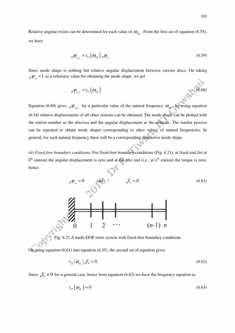
(ii) Fixed-free boundary conditions: For fixed-free boundary conditions (Fig. 6.21), at fixed end (let at

0th station) the angular displacement is zero and at the free end (i.e., at n

th station) the torque is zero,

hence

0

0R zϕ = and 0

R nT = (6.61)

Fig. 6.21 A multi-DOF rotor system with fixed-free boundary conditions

On using equation (6.61) into equation (6.55), the second set of equation gives

22 0 0nf R

t Tω

= (6.62)

Since 0 0RT ≠ for a general case, hence from equation (6.62) we have the frequency equation as

( )220

nft ω = (6.63)

304

It should be noted that for the case when the free end is at 0th station (i.e., at the extreme left) and the

fixed end is at nth station (i.e., at the extreme right), the frequency equation would be (it is assumed

that the free-end and intermediate stations have a disc)

( )110

nft ω = (6.64)

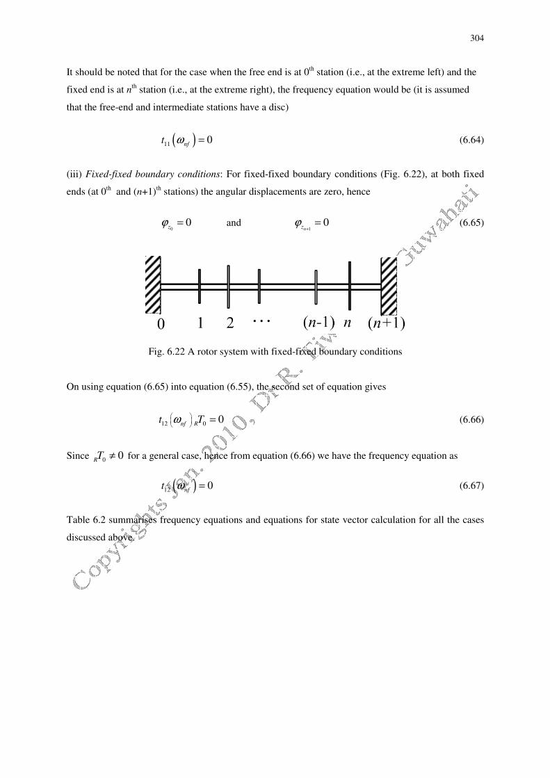
(iii) Fixed-fixed boundary conditions: For fixed-fixed boundary conditions (Fig. 6.22), at both fixed

ends (at 0th and (n+1)

th stations) the angular displacements are zero, hence

0

0z

ϕ = and 1

0nz

ϕ+

= (6.65)

Fig. 6.22 A rotor system with fixed-fixed boundary conditions

On using equation (6.65) into equation (6.55), the second set of equation gives

12 0

0nf R

t Tω

= (6.66)

Since 0

0RT ≠ for a general case, hence from equation (6.66) we have the frequency equation as

( )120

nft ω = (6.67)

Table 6.2 summarises frequency equations and equations for state vector calculation for all the cases

discussed above.

305

Table 6.2 Equations for the calculation of natural frequencies and mode shapes.

S.N. Boundary

conditions

Station

numbers

Equations to get natural

frequencies

Equations to get mode shapes

1 Free-free 0, n+1: Free

ends

( )21 0nf

t ω = ( )1 011n iz nf zR

tϕ ω ϕ+

=

2 Cantilever

(Fixed-free)

0: Fixed

end,

n: free end

0: Fixed

end,

n: free end

( )220

nft ω =

( )110

nft ω =

( )012n iz nf zR

t Tϕ ω=

( )021n iz nf zR

T t ω ϕ=

3 Fixed-fixed 0, n+1:

Fixed ends ( )12

0nf

t ω = ( )1 022n iz nf zR

T t Tω+

=

In above cases we have considered intermediate supports as frictionless, and no friction of discs with

the medium in which these discs are oscillating. In actual practice, we will have supports and discs

with friction, and this will produce some frictional (damping) torque on to the shaft or discs. While

rotor is rotating with at a certain constant spin speed, these supports and discs frictions would give a

constant torque. However, the torque onto the shaft and discs will be function of the spin speed of the

rotor. Overall effects of these frictions would be very less on the torsional natural frequencies of rotor

systems, and for initial estimates of system dynamic characteristics it can be ignored. Torsional

oscillations of the rotor with flexible elements like couplings and torsional dampers will be considered

subsequently.

A word of caution regarding the numbering of stations: for the present formation we stick to the

numbering scheme the 0th station is assigned to the extreme left side of the station, and subsequent

station numbers (i.e., 1, 2, …) are given to the station encountering towards the right. In the case

numbering to the station is from extreme right and increases towards left, then the following point and

field matrices should be used (which are slightly different as compared to equations (6.68) and (6.69))

306

2

1 0

1nf p

PIω

=

� and

1 1

0 1

kF

− =

� (6.70)

where P �

and F �

are the point and field matrices when the transformation of state vector is

performed from the right to the left. For example equations (6.47) and (6.52) can be written as

{ } { }2 22L R

S P S = �

and { } { }1 22R L

S F S = �

(6.71)

with

[ ]1

22P P

− = �

and 1

2 2F F

− = � �

It should be noted that these point and field matrices are in fact inverse of the previous matrices. To

avoid this confusion in the present text the station number is consistently assigned from the left end to

the right end, and the transformation of the state vector is also followed the same sequence (i.e., from

the left to the right). To illustrate the TMM now several simple numerical problems will be taken up.

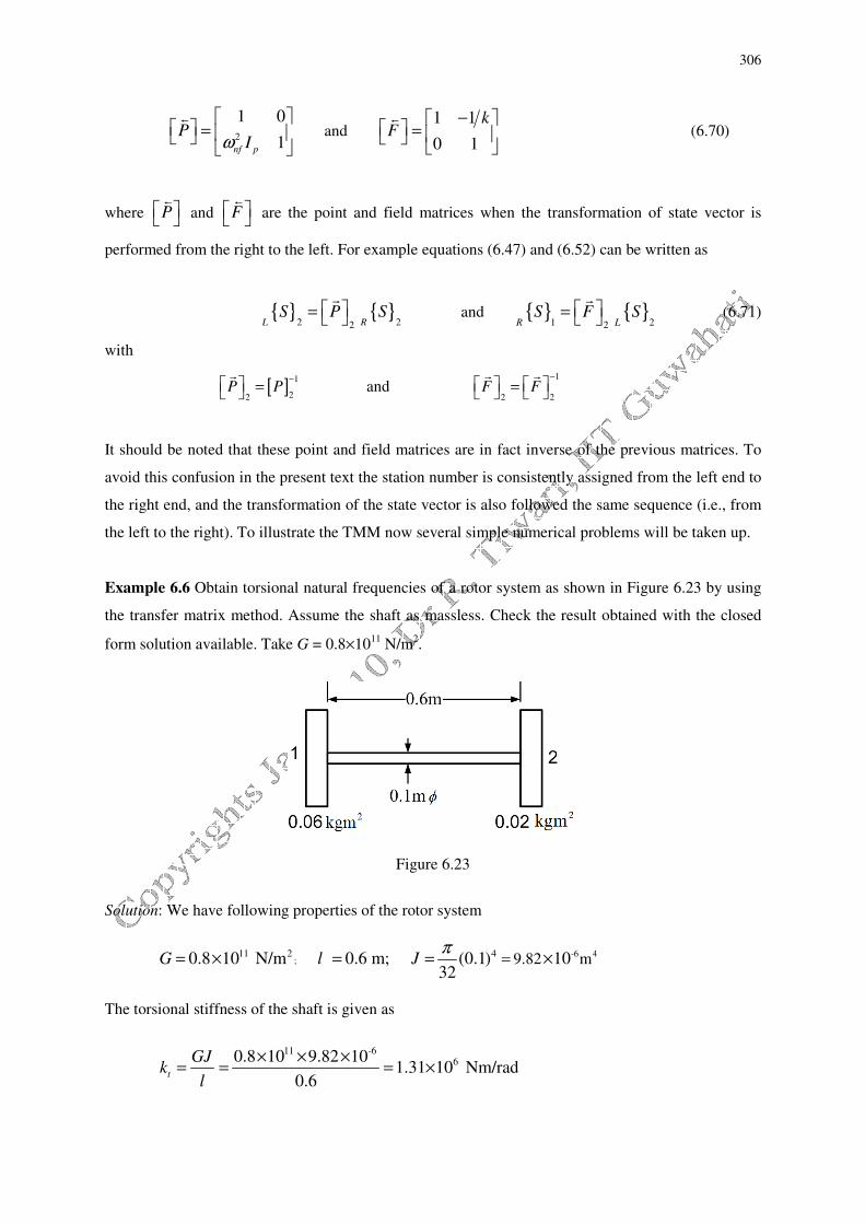
Example 6.6 Obtain torsional natural frequencies of a rotor system as shown in Figure 6.23 by using

the transfer matrix method. Assume the shaft as massless. Check the result obtained with the closed

form solution available. Take G = 0.8×1011

N/m2.

Figure 6.23

Solution: We have following properties of the rotor system

-6 4;

11 2 4 9.82 m0.8 10 N/m 0.6 m; (0.1) 10

32G l J

π== × = = ×

The torsional stiffness of the shaft is given as

-6116

0.8 10 9.82 10

1.31 10 Nm/rad0.6

t

GJk

l

× × ×= = = ×

307

Analytical method: Natural frequencies in the closed form are given as

( )1

1 2

2

1 2

6( ) 0.06 0.02 1.31 100; and 9345.23 rad/sec

0.06 0.02

p p t

nf nf

p p

I I k

I Iω ω

+ + ×= = = =

×

Mode shapes (relative amplitudes) are given as

for 1

0nf

ω = , 2

0

1z

z

Φ=

Φ;

and

for 2

9345.23 rad/snf

ω = , 2 1

0 2

3z p

z p

I

I

Φ= − = −

Φ;

Transfer matrix method: Let the station number be 1 and 2 as shown in Fig. 6.24. State vectors can be

related between stations 1 and 2, as

and

1 1 1

2 2 2 1 2 2 1 1

{ } [ ] { }

{ } [ ] [ ] { } [ ] [ ] [ ] { }

R L

R R L

S P S

S P F S P F P S

=

= =

The overall transformation of state vectors between 1 & 2 is given as

( )

( ){ } ( )

2 1 12 2

1

2 1 2 2

2 2 22 2

2 1 1

2

2 2 2 2

1 11 0 1 0 1 01 1

1 1 110 1

1 1

1 1

tz t z z

nf p nf p nf pnf p nf p tR L L

nf p t tz

Lnf p nf p nf p t nf p t

kk

I I II I kT T T

I k k

TI I I k I k

ϕ ϕ ϕ

ω ω ωω ω

ω ϕ

ω ω ω ω

= = − − −− −

− = − − − − 1

On substituting values of various rotor parameters, it gives

( )

( ) ( )

8 2 7

2 10 4 8 22 1

1 4.58 10 7.64 10

0.08 9.16 10 1 1.53 10

nfz z

R Lnf nf nfT T

ωϕ ϕ

ω ω ω

− −

− −

− × × = − + × − ×

(a)

Since ends of the rotor are free-free type, hence, the following boundary conditions will apply

308

1 2 0

L RT T= = (b)

On application of boundary conditions (b) in equation (a), we get the following condition

( ) ( )2 10 4

21 10.08 9.16 10 { } 0nf nf nf L z

t ω ω ω ϕ−= − + × =

which gives for the non-trial solution, the following frequency equation

2 10 2[9.16 10 0.08] 0nf nfω ω−× − =

It gives natural frequencies as

1 2

0 and 9345.23 rad/secnf nf

ω ω= =

which are exactly the same as obtained by the closed form solution. Mode shapes can be obtained by

substituting these natural frequencies, one at a time, into the first (or the second) expression of

equation (a), as

( )2

01

8 2

0

1 4.58 10 1

nf

z

nf

z ω

ω−

=

Φ= − × =

Φ, rigid body mode

and

( )2

02

8 2

9345.23

1 4.58 10 3

nf

z

nf

z ω

ω−

=

Φ= − × = −

Φ, anti-phase mode

which are also exactly the same as obtained by closed form solutions.

Example 6.7 Obtain torsional natural frequency for a cantilever shaft carrying a disc and a spring at

free end as shown in Figure 6.24. The disc has the polar mass moment of inertia of 0.02 kg-m2. The

shaft has 0.4 m of the length and 0.015m of the diameter. The spring has torsional stiffness of 2t

k =

100 N-m/rad. Take G = 0.8×1011

N/m2 for the shaft.

309

Figure 6.24 A cantilever rotor with a spring at the free end

Solution: Let the fixed end has the station number as 0, the shaft free end has the station number as 1,

and spring other end fixed to the fixed support has the station number 2 (Fig. 6.24). The

transformation of the state vector from station 0 to station 1 can be written as

{ } [ ] [ ] { }1 1

1

2 21 01 1

20 0

11 0 1

1

0 1 1

z z

Rnf p nf p

nf p

ll

GJS P F S GJ

I I lT TI

GJ

ϕ ϕ

ω ωω

= = = − − −

(a)

The spring at free end can be thought as an equivalent shaft segment with same stiffness that of the

spring. The overall transfer matrix for such an idealisation between stations 0 and 2 would be

{ } [ ] [ ] [ ] { }

1 1

2 2

2

11

11

2 2

22 02 1 12

2 0 02

11 1 11

1

10 1 1

nf p nf p

z zt tt

nf pnf p

nf pnf p

I I lll

k GJ k GJGJkS F P F S

I l T TI lI IGJ GJ

ω ω

ϕ ϕ

ω ωω ω

− + − = = = − − − −

(b)

Boundary conditions for the present case would be

0 2

0z zϕ ϕ= = (c)

On applying boundary conditions to equation (b), from first equation, we get

1

2

2

0

11 0

nf p

t

I llT

GJ k GJ

ω + − =

(d)

Since torque T0 can not be zero, hence we get the natural frequency from equation (d) as

2

1

( / )t

nf

p

k GJ l

Iω

+= rad/s (e)

310

with

4 90.015 4.97 1032

Jπ −= = × m

4,

10.02pI = kg-m

2, 994.02

GJ

l= Nm/rad,

2100tk = Nm/rad

Hence, we have natural frequency as

nfω = 233.88 rad/s answer

From equation (e), it can be observed that the effect of the spring at the free end is to increase the

effective stiffness of the system (i.e., springs connected in parallel with the equivalent stiffness of

2( / )tk GJ l+ , where GJ/l is the stiffness of the shaft).

Alternatively, the spring can be included as a boundary condition as follows. In this case the

transformation equation (a) is valid. The equilibrium equation at the free end would be

2 11 0R t zT k ϕ+ = (f)

where RT1 is the reaction toque at the right of disc. Hence, the boundary conditions would be

0

0zϕ = and 2 11R t zT k ϕ= − (g)

On application of boundary conditions (g) in equation (a), we get

2 1

1

2

2 01

10

1

z

t z nf pRnf p

l

GJ

k I l TI

GJ

ϕ

ϕ ωω

=

− − −

(h)

Equation (h) can be split as follows

1 0R z

lT

GJϕ = and 1

2 1

2

01nf p

t R z

I lk T

GJ

ωϕ

− = −

(i)

which gives an eigen value problem of the following form

311

1

1

2

2

0

10

01

z

nf p

t

l

GJ

I l Tk

GJ

ϕ

ω

− = −

(j)

For the non-trial solution, on taking determinant of the above matrix, it gives the natural frequency

exactly same as in equation (e).

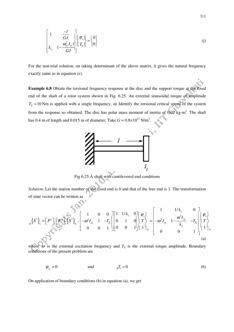
Example 6.8 Obtain the torsional frequency response at the disc and the support torque at the fixed

end of the shaft of a rotor system shown in Fig. 6.25. An external sinusoidal torque of amplitude

10E

T = Nm is applied with a single frequency, ω. Identify the torsional critical speed of the system

from the response so obtained. The disc has polar mass moment of inertia of 0.02 kg-m2. The shaft

has 0.4 m of length and 0.015 m of diameter. Take G = 0.8×1011

N/m2.

Fig 6.25 A shaft with cantilevered end conditions

Solution: Let the station number of the fixed end is 0 and that of the free end is 1. The transformation

of state vector can be written as

{ } { }

1

1

1

1 1 1 1

1

2

* * * * 2 2

1 11 0

0 0

1 1/ 01 1/ 01 0 0

1 0 1 0 1

0 0 1 1 10 0 10 0 1

t

t z z

p

p E p ER

t

kk

II T T I T T

kS P F S

ϕ ϕω

ω ω=

− − = − − −

=

(a)

where ω is the external excitation frequency and TE is the external torque amplitude. Boundary

conditions of the present problem are

00zϕ = and 1 0

RT = (b)

On application of boundary conditions (b) in equation (a), we get

312

1

1

1 1

1

2

2

1 0

1 1/ 00

0 1

1 10 0 1

t

z

p

p E

t

R

k

II T T

k

ϕω

ω

= − − −

(c)

which gives following equations

1

1

0

R z

t

T

kϕ = and 1

1

1

2

00 1p

E

t

IT T

k

ω = − −

(d)

From above, the frequency response at station 1 would take the following form

1 1

1

1

1

2 2

211

E E

R z

p

nft

T T

I

k

ϕω ω

ω

= =

−−

with /nf t p

k Iω = (e)

For the present problem 1

10ET = Nm, 94.97 10J−= × m

4,

10.02pI = kg-m

2,

1994.02

t

GJk

l= = Nm/rad,

and hence 222.94nfω = rad/s.

Hence from equations (e) and (d), we have

1 2

4

10

14.97 10

R zϕω

=

− ×

rad and 0 2

4

10 994.02

14.97 10

Tω

×=

− ×

(f)

Equation (f) can be used to plot the amplitudes of the frequency response at the disc and the reactive

toque at the fixed support with respect to the excitation frequency, ω . However, it can be seen from

the denominator that the resonance takes place when it becomes zero, i.e., 222.94nfω ω= = rad/s,

which is the condition of critical speed, 222.94cr

ω ω= = rad/s.

313

Example 6.9 Find torsional natural frequencies and mode shapes of a rotor system shown in Figure

6.26. B is a fixed end, and D1 and D2 are rigid discs. The shaft is made of steel with the modulus of

rigidity G = 0.8 (10)11

N/m2 and a uniform diameter d = 10 mm. Shaft lengths are: BD1 = 50 mm, and

D1D2 = 75 mm. Polar mass moment of inertia of discs are: 1pI = 0.08 kg-m

2 and

2pI = 0.2 kg-m2.

Consider the shaft as massless and apply (i) the analytical method, and (ii) the transfer matrix method.

Figure 6.26

Solution: The torsional free vibration would be done by classical analytical method and the TMM to

have comparion of results.

Analytical method: From free body diagrams of discs as shown in Figure 6.27, equations of motion

for free vibrations can be written as

1 1 1 1 21 2 ( - ) 0p z z z z

I k kϕ ϕ ϕ ϕ+ + =�� and 2 2 2 12 ( - ) 0

p z z zI kϕ ϕ ϕ+ =�� (a)

Equations of motion are homogeneous second order differential equations. In free vibrations, discs

will execute simple harmonic motions.

Figure 6.27 Free body diagrams of discs

For the simple harmonic motion, 2 2 sinz nf z nf z nf tϕ ω ϕ ω ω= − = − Φ�� , hence equations of motion take

the form

314

11

22

2

1 2 2

2

2 2

- 0

0

zp nf

zp nf

k k I k

k k I

ω

ω

Φ + − =

Φ− − (b)

On taking determinant of the above matrix, it gives the frequency equation as

1 2 1 2 2

4 2

2 1 2 1 2( ) 0p p nf p p p nfI I I k I k I k k kω ω− + + + = (c)

which can be solved for 2

nfω , as

( )1 2 2 1 2 2 1 2

1 2

2

2 1 2 2 1 2 1 224

2

p p p p p p p p

nf

p p

I k I k I k I k I k I k k k I I

I Iω

+ + ± + + −= (d)

For the present problem following properties are given

( ) 4. . m J d Jπ π −= = = × =

44 4

1 20 01 9 82 10

32 32

1 21 2

1 2

1570.79 N/m and 1047.19 N/mGJ GJ

k kl l

= = = =

1 2

2 20.08 kgm and 0.2 kgmp pI I= =

From equation (d), natural frequencies are obtained as

1 2

54.17 rad/s and 187.15 rad/snf nf

ω ω= =

The relative amplitude ratio can be obtained from the first expression of equation (b), as

1

1 2

2 1

2

2

1 2

0.4394 for ; and -5.689 for -

z

nf nf

z p nf

k

k k Iω ω

ω

Φ= =

Φ + (e)

Alternatively, the relative amplitude ratio can be obtained from the second expression of equation (b),

as

1 2

1 2

2

2

2

2

-0.4394 for ; and -5.689 for

z p nf

nf nf

z

k I

k

ωω ω

Φ= =

Φ (f)

As expected it should give the same result as in equation (e). Mode shapes are shown in Figure 6.28.

In which the first one is in-phase mode and second is the anti-phase mode. Practically, the anti-phase

315

mode is difficult to excite (more resistive torque) as compared to the in-phase mode, and because of

this the natural frequency of the former mode is more than the latter.

Figure 6.28 Mode shapes

Transfer matrix method

Figure 6.29 Two-discs rotor system with numbering of stations

For Figure 6.29, state vectors between 0th and 2

nd stations can be related as

{ } [ ] [ ] [ ] [ ] { }2 2 2 1 1 0R

S P F P F S= (g)

State vectors at neighbouring stations (i.e., 1 and 2, and 0 and 1) can be related as

2 1

2 1

2 1

2 2

2 2

2 1 1 0

1 1

1 1/ 1 1/

and- 1 - 1

z z z z

nf p nf p

nf p nf pR R R R

k k

I IT T T TI I

k k

ϕ ϕ ϕ ϕω ω

ω ω

= =− − + +

(h)

which can be combined to give

1 1

2 2

2 1

2 2

2 1 2 2

2 22 02 2 21

2 1 2

1 11- 1

1 1

nf p nf p

z z

R nf p nf p

nf p nf p

I I

k k k k

T TI ItI I

k k k

ω ω

ϕ ϕ

ω ωω ω

− +

= −

− − + − +

(i)

1

-5.68

0

(b) 2

For n

ω

0

1

0.4394

(a) 1

For n

ω

316

Boundary conditions are: at station 0, zϕ =0

0 ; and at right of station 2, RT =

20 . On application of

boundary conditions in equation (i), the second equation gives the frequency equation as

( ) 2 2

2 1

2 2

2 2

22

1 2 2

11 1 0

nf p nf p

nf nf p nf p

I It I I

k k k

ω ωω ω ω

−= − − + − + =

which can be simplified as

1 2 1 2 2

4 2

2 1 2 1 2( ) 0p p nf p p p nfI I I k I k I k k kω ω− + + + =

It should be noted that it is same as obtained by the analytical method in equation (c). Hence, natural

frequencies by TMM will be also given by equation (d). For obtaining mode shapes from equations

(h) and (i), we have

2 12 0R z t Tϕ = ;

2 1

1

2

R

R z R z

T

kϕ ϕ= + ;

1

0

1

R z

T

kϕ = (j)

From equation (j), we have

1 1

2 2 1

2

2

1 12 1 2

1R z R z

R z R z p nf

k

k t k k I

ϕ

ϕ ω

Φ= = =

Φ + − (k)

which is again same as equation (e). Since mode shapes are relative angular displacements of various

discs in the rotor system, on assuming one of the angular displacement as unity (i.e., zϕ =2

1), we can

get torque acting at various sections of the shaft from equation (j), as

( )

1 2 1 2

20 2 2

12 2 2

1

nf p p p p nf

kT

t k I k I I Iω ω= =

+ − (l)

and

( )( )2 1

1 2 1 2

0 21 2 2 2 2 2

1 1 2 2

1 1R R z R z

nf p p p p nf

T kT k k k

k k k I k I I Iϕ ϕ

ω ω

= − = − = −

+ −

(m)

It should be noted that these torques would be produced for a unit angular displacement at disc 2 (i.e.,

zϕ =2

1).

317

Example 6.10 Find torsional natural frequencies and mode shapes of the rotor system shown in

Figure 6.30. B1 and B2 are frictionless bearings, which provide free-free end condition; and D1, D2, D3

and D4 are rigid discs. The shaft is made of the steel with the modulus of rigidity G = 0.8 (10)11

N/m2

and a uniform diameter d = 20 mm. Various shaft lengths are as follows: B1D1 = 150 mm, D1D2 = 50

mm, D2D3 = 50 mm, D3D4 = 50 mm and D4B2 = 150 mm. The mass of discs are: m1 = 4 kg, m2 = 5 kg,

m3 = 6 kg and m4 = 7 kg. Consider the shaft as mass-less. Consider discs as thin and take diameter of

discs as d =1

8 cm, d =2

10 cm, d =

312 cm, and

d =

414 cm.

Figure 6.30 A multi-disc rotor system

Solution: The discs have the following data

m1 = 4 kg, m2 = 5 kg, m3 = 6 kg, m4 = 7 kg

.d =1

0 08 m, .d =2

0 1m,

.d =3

0 12 m, .d =4

0 14 m,

1

1 12 2

1 12 24 0.04 0.0032pI m r= = × × = kg-m

2,

2

1 2

25 0.05 0.00625pI = × × = kg-m

2,

3

1 2

26 0.06 0.0108pI = × × = kg-m

2,

4

1 2

27 0.07 0.01715pI = × × = kg-m

2,

The shaft has GJ = 1256.64 N-m2 and following dimensions according to station numbers (1, 2, 3 and

4 are given station numbers at disc locations; shaft segments at ends will not contribute in the free

vibration for the present case)

l1 = 50 mm, l2 = 50 mm, l3 = 50 mm

Now the overall transformation of the state vector can be written as

{ } [ ] { }4 1R L

S T S= (a)

with

318

[ ] [ ] [ ] [ ] [ ] [ ] [ ] [ ]4 3 3 2 2 1 1

T P F P F P F P= (b)

[ ] 2

1 0

1i

inf p

PIω

= −

; [ ]1 1

0 1

it

i

kF

=

; { } zS

T

ϕ =

(c)

From Table 6.2, for free-free boundary conditions the frequency equation is

( ) ( )2,1 0nf nf

f tω ω= = (d)

On solving the roots of above function by the root searching method, it gives the following natural

frequencies

1nfω = 0 rad/s, 2nfω = ?? rad/s,

2nfω = ?? rad/s, 4nfω = ?? rad/s,

From Table 6.2, the eigen vector can be obtain from the following equation

( )4 111 iz nf zR

tϕ ω ϕ= (e)

Now on choosing 1

1z

ϕ = as reference value and let us obtain the state vectors corresponding to the

second mode, i.e. 2inf nf

ω ω= ). From equations (e) and noting the boundary condition, we get the state

vector at 1st and 4

th station as

1

1{ }

0L S

=

; and ( )

211

4

?{ }

00

nf

RS

t ω = =

At other stations also the state vectors can be obtained as

[ ]1 11

?{ } { }

?R LS P S

= =

; [ ]2 11

?{ } { }

?L RS F S

= =

and

[ ]2 22

?{ } { }

?R LS P S

= =

; [ ]3 22

?{ } { }

?L RS F S

= =

319

[ ]3 33

?{ } { }

?R LS P S

= =

; [ ]4 33

?{ } { }

?L RS F S

= =

Hence, the mode shape (the relative angular displacement) can be drawn as shown in Fig. 8.31 for the

second modes? On the same lines other state vectors corresponding to remaining natural frequencies

can be obtained to get the related mode shapes as shown in Fig.8.31?.

320

6.6 Geared Systems

In actual practice, it is rare that the rotor system has a single shaft (with either uniform or stepped

cross sections) with multiple discs as we analysed in previous sections. In some machine the shaft

may not be continuous from one end of the machine to the other, but may have a gearbox installed at

one or more locations. Hence, shafts will be having different angular velocities as shown in Figure

6.30(a). For the purpose of analysis the geared system must be reduced to system with a continuous

shaft so that they may be analysed for torsional vibrations by methods as described in preceding

sections.

Fig. 6.30 (a) Actual geared system (b) An equivalent system without geared system (c) The equivalent

system with disc 2 as fixed and (d) The equivalent system with shaft 2 as rigid

It is assumed that gears and shafts have negligible polar mass moment of inertia as compared to discs

in the geared rotor system. In the actual system as shown in Figure 6.30(a), k2 is the torsional stiffness

of the shaft between gear 2 and disc 2, and 2pI is the polar mass moment of inertia of disc 2. Let the

equivalent system as shown in Fig. 6.30(b) has the shaft torsional stiffness ke and the disc mass

moment of inertia eP

I . The strain and kinetic energy values must be the same in both the real and

dynamically equivalent systems for the theoretical model to be valid.

Equivalent stiffness: Let the disc with the polar mass moment of inertia, pI

2, is imagined to be held

rigidly in both the real and equivalent (Fig. 6.30c) systems, while the pinion shaft 1 is rotated through

321

an angle of z

ϕ1 at the input to gearbox (i.e., at the pinion). Shaft 2 is rotated through an angle

/z z

nϕ ϕ=2 1

at the gear 2, where n is the gear ratio. It is the ratio of the angular speed of the driving

gear (pinion) to that of the driven gear, i.e.

( )( )

z

z

t Nn

t N

ϕω

ω ϕ= = =1

2

1 2

2 1

where ω is the spin speed of the gear and N is the number of teeth of the gear. The speed ratio, train

value, and kinematic coefficient are other terms used for gear ratio, however, these are inverse of the

gear ratio, i.e. the ratio of the angular speed of the driven gear to that of the driving gear. Hence, the

strain energy stored in shaft 2 of the actual system, for a twist of z

ϕ1 at the input to the gear box, can

be written as

1

2

1 12

2 22 2

2

z

r zn

U k kϕ

ϕ

=

= (6.72)

where Ur is the strain energy in the real system. While applying the same input at the gear box to the

equivalent system (Fig. 6.30c) results in the stain energy stored in the equivalent shaft, and can be

expressed as

1

1 12 2

2 2ee z ze eU k kϕ ϕ== (6.73)

where Ue is the strain energy in the equivalent system, and since we have ez z

ϕ ϕ=1. On equating

equations (6.72) and (6.73), it gives the equivalent stiffness as

2

2ek

nk = (6.74)

Equivalent polar mass moment of inertia: Now we consider the shaft 2 as a rigid shaft in both the real

and equivalent systems (Fig. 6.30d), so that angular motion of gear 2 and disc 2 is same. That means

whatever motion at pinion is given to: (i) the real system disc 2 gets same motion as the gear 2, (ii) for

the equivalent system disc 2 gets same motion as the pinion itself. Kinetic energies of both the real

and equivalent systems must also be equated

1 2

22 2r p

T I ω= and 1 2

2e p ee

T I ω= (6.75)

322

where Tr and Te is the kinetic energies in the real and equivalent system, respectively; 2

ω and e

ω are

angular frequencies of disc 2 of the real (2pI ) and equivalent (

epI ) systems, respectively. Equations

(6.75) can be equated and is written as

( ) ( )2

1 1

2 12 22

22

ep pz zeI Iω ϕ ω ϕ+ = +� � (6.76)

where 2zϕ and

ezϕ are the angle of twist of shaft 2 in the actual and equivalent systems, respectively.

It can be seen from Figure 6.30(d) that ezϕ =

1zϕ and ω1 and ω2 are angular frequencies of the shaft 1

and 2, respectively. We have the following basic relations

1 2

1 2 1

2 2

and ez z z

e

T T nT

k k kϕϕ ϕ= = = = (6.77)

where T1 and T2 are torques at gears 1 and gear 2, respectively, in actual system. Noting equation

(6.77), equation (6.76) can be written as

2

22

11 1 112

2

1

2 ep p

e

nT Td dI I

n dt k dt k

ωω

+ +

= (6.78)

where T1 is the torque input to the pinion (shaft 1). On substituting equation (6.74) in equation (6.78),

we get

2

2

21 11 1

12 222

2

1ep p

nTd d n TI I

kn dt k dt

ωω

+ +

= ⇒

2 2

2 1 11 1

2 2

2 2

2 e

p

p

n T n Td d

dt k dt k

II

nω ω

+ +

=

which simplifies to

2

2e

p

p

I

nI = (6.79)

where ke and epI are, respectively, the equivalent shaft stiffness and the equivalent polar mass

moment of inertia of the geared system referred to the ‘reference shaft’ speed, i.e. shaft 1. The general

rule, for forming the equivalent system for the purpose of analysis, is to divide all shaft stiffness and

rotor polar mass moment of inertia of the geared system by n2 (where n is the gear ratio). When

analysis is completed, it should be remembered that the elastic line of the mode shape of the

equivalent system (i.e., the line abc in Fig 6.31) is modified for the real system by dividing the

displacement amplitudes of the equivalent shaft by the gear ratio n as shown in Figure 6.31 by the line

abde. It should be noted that angular displacements shown in Fig. 6.31 are now that of discs 1and 2.

323

Figure 6.31 The elastic line in the equivalent and original systems

Example 6.11 For a geared system as shown in Figure 6.32, find torsional natural frequencies and

mode shapes. Find also the location of the node point on the shaft (i.e., the location of the point where

the angular twist during torsional vibrations is zero). The shaft ‘A’ has the diameter of 5 cm and the

length of 0.75 m, and the shaft ‘B’ has the diameter of 4 cm and the length of 1.0 m. Take the

modulus of rigidity of the shaft G = 0.8 × 1011

N/m2, the polar mass moment of inertia of discs are

ApI = 24 Nm

2 and

BpI = 10 Nm

2. Neglect the inertia of gears.

Figure 6.32 A two-disc geared system

Solution: On taking shaft B as the input shaft (or the reference shaft) as shown in Figure 6.33, the gear

ratio can be defined as

Input shaft speed 20Gear ratio 2

Output shaft speed 10

B A

A B

Dn

D

ω

ω= = = = = =

where D is the nominal diameter of the gear.

324

Figure 6.33 A geared system

The polar moment of inertia of the shaft cross-section and the torsional stiffness of the shaft can be

obtained as

4 7 4 4 7 4π π6.136 10 m ; 2.51 10 m

32 32A A B B

J d J d− −= = × = = × ;

and 11 -7

4 40.8 10 6.136 106.545 10 Nm/rad; 2.011 10 Nm/rad

0.75

AA B

A

GJk k

l

× × ×= = = × = × ;

On treating as a reference shaft to the shaft B and replacing an equivalent shaft system of shaft A (i.e.,

the same diameter as that of reference shaft B), the system will become as shown in Figure 6.34. The

equivalent system of the shaft system A has the following torsional stiffness and polar mass moment

of inertia properties

44 2

2 2 22

246.545 101.6362 10 Nm/rad and 6 Nm

2 2A

A

PA

A Pe

kk

n

II

n=

×= = = × = =

which gives the equivalent length of shaft A as (note that now its diameter is that of the reference shat

B)

11 7

41.229m

0.8 10 2.513 10

1.6362 10e

BA

Ae

lk

GJ−× × ×

= = =×

.

Hence, the equivalent full shaft length is given as e 1.229 1 2.229 mA B

el l l= + = + = .

325

Figure 6.34 An equivalent single-shaft geared system

The equivalent stiffness of the full shaft is given as (Fig. 6.34)

4

4 4

1 1rad/Nm

2.011 10 1.6362 10

1 1 11.1085 10

e A Be

k k k

−= +× ×

= + = ×

which gives 9021.2 Nm/rade

K = . The flexible natural frequency of the equivalent two-disc rotor

system as shown in Figure 6.34 is given as

( )

( )2 2

( ) 6 10 9021.2/9.81=153.62 rad/sec

( ) 6 10 /9.81

A Be

A Be

P P e

nf

P P

I I k

I Iω

+ + ×= =

×

Figure 6.35 Mode shape and nodal point location in the equivalent system

The node location can be obtained from Figure 6.35 as

1 2

Ae Bz z

n nl l

Φ Φ=

which can be written by noting equation (6.13), as

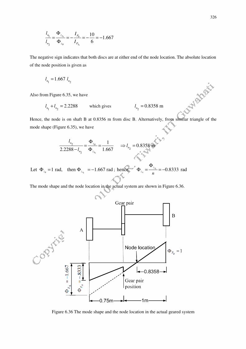
326

1

2

101.667

6

Ae B

B Ae

n z P

n z P

l I

l I

Φ= = − = − = −

Φ

The negative sign indicates that both discs are at either end of the node location. The absolute location

of the node position is given as

1 21.667

n nl l=

Also from Figure 6.35, we have

1 22.2288

n nl l+ = which gives

20.8358 m

nl =

Hence, the node is on shaft B at 0.8356 m from disc B. Alternatively, from similar triangle of the

mode shape (Figure 6.35), we have

2

2

2

1 0.8358 m

2.2288 1.667

B

Ae

n z

n

n z

ll

l

Φ= = ⇒ =

− Φ

Let 1 rad, then 1.667 radB Ae

z zΦ = Φ = − ; hence, 0.8333 radAe

A

z

zn

ΦΦ = = −

The mode shape and the node location in the actual system are shown in Figure 6.36.

Figure 6.36 The mode shape and the node location in the actual geared system

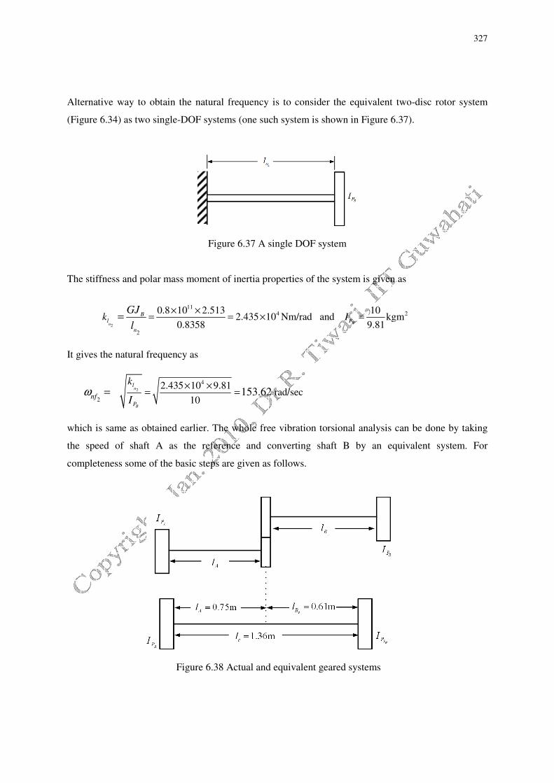
327

Alternative way to obtain the natural frequency is to consider the equivalent two-disc rotor system

(Figure 6.34) as two single-DOF systems (one such system is shown in Figure 6.37).

Figure 6.37 A single DOF system

The stiffness and polar mass moment of inertia properties of the system is given as

2

114 2

2

0.8 10 2.513 102.435 10 Nm/rad and kgm

0.8358 9.81Bn

Bl P

n

k IGJ

l

× ×= = × ==

It gives the natural frequency as

2

4

2

2.435 10 9.81 rad/sec

10153.62

n

B

l

P

nf

k

Iω

× ×= ==

which is same as obtained earlier. The whole free vibration torsional analysis can be done by taking

the speed of shaft A as the reference and converting shaft B by an equivalent system. For

completeness some of the basic steps are given as follows.

Figure 6.38 Actual and equivalent geared systems

328

The gear ratio for the present case will be

100.5

20

A B

B A

Dn

D

ω

ω= = = =

It is assumed that equivalent shaft (i.e., the shaft B) has the diameter same as that of the reference

shaft (i.e., the shaft A). The equivalent polar mass moment of inertia and the torsional stiffness can be

written as

4

2 4

2 2 2

2.011 1040 Nm and 8.044 10 Nm/rad

(0.5)

B

Be

P BP Be

I kI k

n n

×= = = = = ×

which gives the equivalent length as

11 74

4

0.8 10 6.136 108.044 10 Nm/rad 0.610 m

8.044 10

AB B

Be

e

e

GJk l

l

−× × ×= = × ⇒ = =

×

The total equivalent length and the equivalent torsional stiffness would be

eA Be 0.75 0.61 1.36 ml l l= + = + =

and 11 7

40.8 10 6.136 103.61 10 Nm/rad

1.360

A

e

kGJ

el

−× × ×= = = ×

Alternatively, the effective stiffness can be obtained as

1 1 1

A Be

k k ke= + ⇒

4 44

4 4

6.545 10 8.044 103.61 10 Nm/rad

6.545 10 8.044 10

A B

A B

e

e

k kke

k k

× × ×= = = ×

+ × + ×

Natural frequencies of two mass rotor system are given as

1 0nfω = and 4

2

( ) (24 40)9.81 3.61 10

24 40153.62 rad/s

A Be

A Be

P P

nf e

P P

I Ik

I Iω

+ += × × ×

×= =

A factor 9.81 is used since API is in Nm

2 and we need in kgm

2.

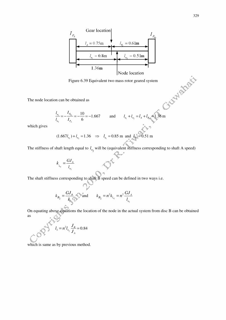
329

Figure 6.39 Equivalent two mass rotor geared system

The node location can be obtained as

1

2

101.667

6

Be

A

Pn

n P

Il

l I= − = − = − and

1 21.36

en n A Bl l l l+ = + = m

which gives

1 2 1 2

(1.667 ) 1.36 0.85 m and 0.51 m n n n nl l l l+ = ⇒ = =

The stiffness of shaft length equal to 2

nl will be (equivalent stiffness corresponding to shaft A speed)

2

2

n

A

l

n

GJ

lk =

The shaft stiffness corresponding to shaft B speed can be defined in two ways i.e.

22

B

BkGJ

l= and

2

2

2 2

2 n

Al

n

Bk kGJ

n nl

= =

On equating above equations the location of the node in the actual system from disc B can be obtained

as

2

2

2 0.84B

n

A

Jl n l

J==

which is same as by previous method.

330

6.7 TMM for Branched Systems

For rolling mills, textile machineries, the marine vessel power transmission shafts, and machine tool

drives; there may be many rotor inertias in the system and gear box may be a branch point where

more than two shafts are attached. In such cases where there are more than two shafts attached as

shown in Fig. 6.40 to the gearbox, the system is said to be branched. It has three braches A, B and C;

and each branch has multiple discs, e.g. p, q, and r number of discs (including gears) in branches A, B

and C, respectively. Such system can not be converted to a single shaft system as we could do to the

two-shaft geared system as discussed in previous section. Since now the system contain several discs

hence, it is a multi-DOF system and hence the analysis of the branched system would now be done by

more general procedure, i.e. the TMM.

Fig. 6.40 A branched multi-DOF rotor system

For the branched system as shown in Figure 6.40, state vectors for different branches can be written as

{ } [ ]{ } { } [ ]{ } { } [ ]{ } 0 0 0

; ; R R RApA rCqB B CS A S S B S S C S= = = (6.80)

where [A], [B], and [C] are overall transfer matrices for branches A, B, and C; respectively.

Branch A: For branch A, taking Azϕ =

01 as the reference value for the angular displacement and since

the left hand end of branch A is free end, hence for free vibrations we have T0A = 0. Equation for

branch A takes the form

11 12

21 22

1

0

z

pA

a a

a aT

ϕ

= (6.81)

331

which can be expanded as

21 11and

pA pAz zT a aϕ= = (6.82)

Branch B: At branch point, between shafts A and B, we have

0

11pA

B

z

z

AB AB

a

n n

ϕϕ == (6.83)

where nAB is the gear ratio between shafts A and B. For branch B, TqB = 0, since the right hand end of

the branch is free. For branch B from equation (6.80), and noting condition described by equation

(6.83), we have

11 12 11

21 22 00

z AB

qB B

b b a n

b b T

ϕ

= (6.84)

Equation (6.84) can be expanded as

1111 012qBz B

AB

a

nb b Tϕ = + (6.85)

and

11 21 11 22

22

21 0 00AB AB

B B

a b a

n b nb b T T

= + ⇒ = − (6.86)

Branch C and junction point: At branch C, we have the following condition (noting equation (6.82))

0

11pA

C

z

z

AC AC

a

n nϕ

ϕ= = (6.87)

where nAC is the gear ratio between shafts A and C. Another condition at the branch to be satisfied

regarding work done by the torque transmitted at various branches (assuming negligible friction

during transmissions), i.e.

0 0

1 1 1

2 2 20 0nA B Cz z zpA B CT T Tϕ ϕ ϕ= +

0 0

0 0 0 0

pA B pA C

B C B C

z z z z AB AC

pA pA

T T T TT T

n nϕ ϕ ϕ ϕ⇒ = + ⇒ = +

(6.88)

On substituting equation (6.86) into the third expression of equation (6.88), it can be written as

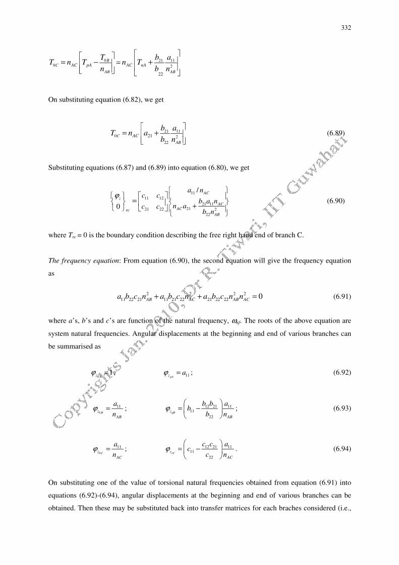
332

0 21 110 2

22

B

C

AB AB

AC pA AC nA

T b aT n T n T

n b n

=

= − +

On substituting equation (6.82), we get

21 110 2

22

21C

AB

AC

b aT n a

b n

= + (6.89)

Substituting equations (6.87) and (6.89) into equation (6.80), we get

11

11 12

21 112121 22 2

22

/

0

AC

z

ACAC

ABrc

a nc c

b a nn ac c

b n

ϕ

+

= (6.90)

where Trc = 0 is the boundary condition describing the free right hand end of branch C.

The frequency equation: From equation (6.90), the second equation will give the frequency equation

as

2 2 2 2

22 11 21 22 21 22 2211 21 0AB AC AB AC

a b c n a b c n a b c n n+ + = (6.91)

where a’s, b’s and c’s are function of the natural frequency, ωnf. The roots of the above equation are

system natural frequencies. Angular displacements at the beginning and end of various branches can

be summarised as

01

Azϕ = ; 11pAz aϕ = ; (6.92)

0

11

Bz

AB

a

nϕ = ; 12 21 11

11

22qBz

AB

b b ab

b nϕ

= −

; (6.93)

0

11

Cz

AC

a

nϕ = ; 12 21 11

11

22rCz

AC

c c ac

c nϕ

= −

. (6.94)

On substituting one of the value of torsional natural frequencies obtained from equation (6.91) into

equations (6.92)-(6.94), angular displacements at the beginning and end of various branches can be

obtained. Then these may be substituted back into transfer matrices for each braches considered (i.e.,

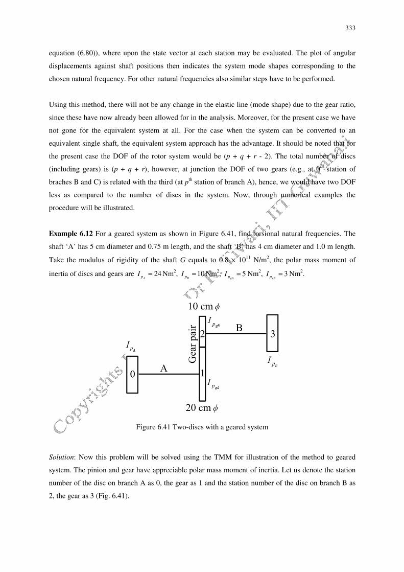
333

equation (6.80)), where upon the state vector at each station may be evaluated. The plot of angular

displacements against shaft positions then indicates the system mode shapes corresponding to the

chosen natural frequency. For other natural frequencies also similar steps have to be performed.

Using this method, there will not be any change in the elastic line (mode shape) due to the gear ratio,

since these have now already been allowed for in the analysis. Moreover, for the present case we have

not gone for the equivalent system at all. For the case when the system can be converted to an

equivalent single shaft, the equivalent system approach has the advantage. It should be noted that for

the present case the DOF of the rotor system would be (p + q + r - 2). The total number of discs

(including gears) is (p + q + r), however, at junction the DOF of two gears (e.g., at 0th station of

braches B and C) is related with the third (at pth station of branch A), hence, we would have two DOF

less as compared to the number of discs in the system. Now, through numerical examples the

procedure will be illustrated.

Example 6.12 For a geared system as shown in Figure 6.41, find torsional natural frequencies. The

shaft ‘A’ has 5 cm diameter and 0.75 m length, and the shaft ‘B’ has 4 cm diameter and 1.0 m length.

Take the modulus of rigidity of the shaft G equals to 0.8 × 1011

N/m2, the polar mass moment of

inertia of discs and gears are 24ApI = Nm

2, 10

BpI = Nm2, 5

gApI = Nm2, 3

gBpI = Nm2.

Figure 6.41 Two-discs with a geared system

Solution: Now this problem will be solved using the TMM for illustration of the method to geared

system. The pinion and gear have appreciable polar mass moment of inertia. Let us denote the station

number of the disc on branch A as 0, the gear as 1 and the station number of the disc on branch B as

2, the gear as 3 (Fig. 6.41).

334

The state transformation equation for the branch A can be written as

{ } [ ] { }1 0R L

S A S= (a)

with

[ ] [ ] [ ] [ ] 2

21 1 0 2

0

1

1 1/

1

1 0

1gA

AgA

A

nf p

nf pnf p

A

k

IA P F PI

kI

ωω ω

= = − −

−

( ) ( )

2

2 2

2 2

11

1 1

A

gA gA

gA A

nf p

A A

nf p nf p

nf p nf p

A A

I

k k

I II I

k k

ω

ω ωω ω

−

=

− + − − −

(b)

where kA is the stiffness of shaft A. Similarly, the state transformation equation for the branch B can

be written as

{ } [ ] { }3 2R L

S B S= (c)

with

[ ] [ ] [ ] [ ]

( ) ( )

2

3 3 2 2 2

2 2

11

1 1

gB

B B

B gB

nf p

B B

nf p nf p

nf p nf p

B B

I

k kB P F P

I II I

k k

ω

ω ωω ω

−

= ==

− + − − −

(d)

where kB is the stiffness of shaft B. At the gear pair, the following conditions hold

1

2

x

xn

ϕϕ = and

2 1T nT= (e)

where ϕx is the angular displacement. Equation (e) can be combined as

2 1

1/ 0

0

x x

L R

n

T n T

ϕ ϕ =

(f)

or

{ } [ ] { }2 1L R

S n S= (g)

335

with the gear ratio transformation matrix is given as

[ ]1/ 0

0

nn

n

=

(h)

Noting equation (g), equation (c) can be written as

{ } [ ][ ] { }3 1R R

S B n S= (i)

Noting equation (a), equation (i) can be expressed as

{ } [ ][ ][ ] { } [ ] { }3 0 0R L L

S B n A S T S= = (j)

with the overall transformation matrix is given as

[ ] [ ][ ][ ]

11 11 12 1121 12 22 12

11 12 11 12

21 22 21 22 11 21 12 2121 22 22 22

1/ 0

0

a b a bna b na b

b b a an n nT B n A

b b a an a b a bna b na b

n n

+ +

= = = + +

(k)

The overall transformation matrix can also be written as

[ ] [ ][ ][ ] [ ] [ ] [ ] [ ][ ] [ ] [ ]3 3 2 1 1 0

T B n A P F P n P F P= = (l)

Boundary conditions of the problem are 0 3

0T T= = since both ends are free. Equation (j) can be

written in expended form as

11 12

21 223 0

x x

R L

t t

t tT T

ϕ ϕ =

or

11 12

21 223 00 0

x x

R L

t t

t t

ϕ ϕ =

(m)

which gives frequency equation as

( )21 0nf

t ω = (n)

From equation (k), frequency equation comes out to be

2

11 21 21 22 0a b n a b+ = (o)

Noting equations (b) and (d), in the expanded form equation (o) can be written

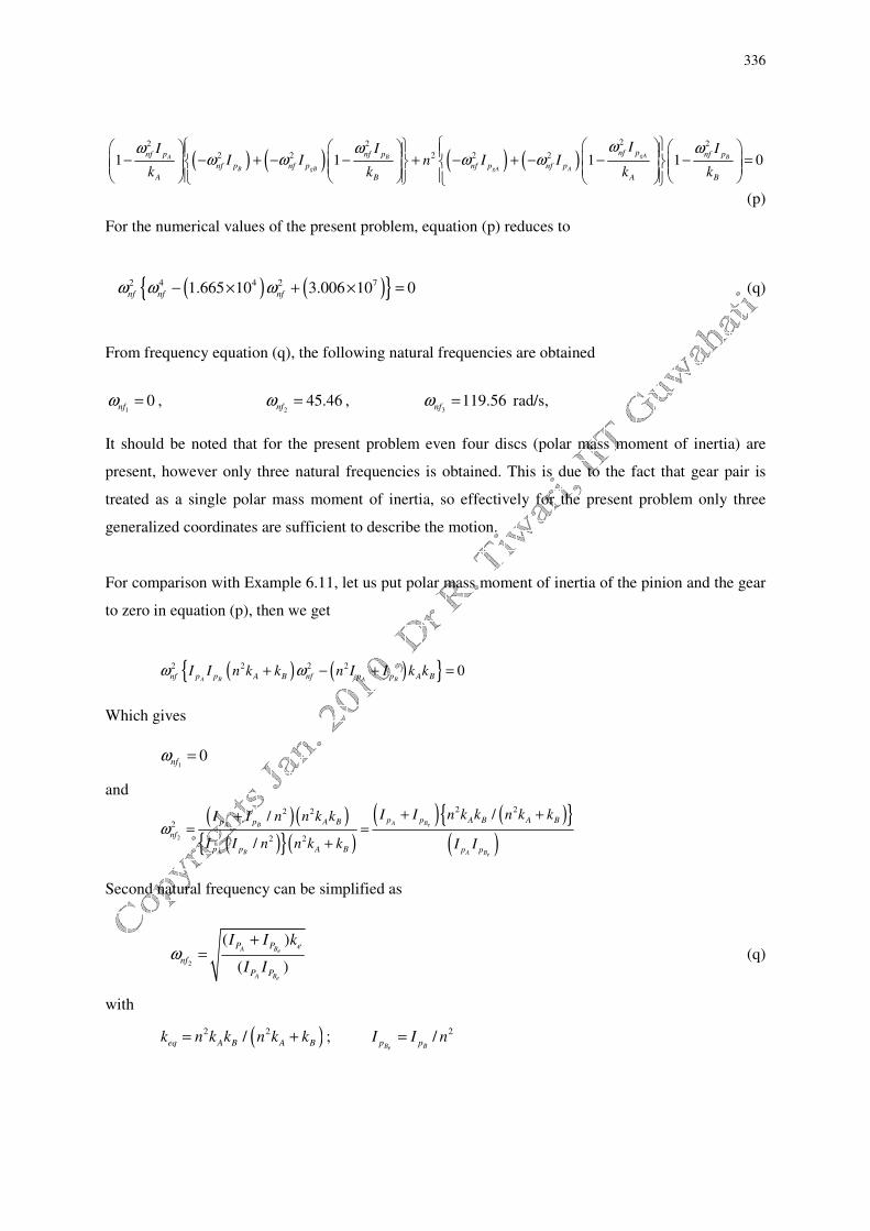
336

( ) ( ) ( ) ( )22 2 2

2 2 2 2 21 1 1 1 0gAA B B

B gB gA A

nf pnf p nf p nf p

nf p nf p nf p nf p

A B A B

II I II I n I I

k k k k

ωω ω ωω ω ω ω

− − + − − + − + − − − =

(p)

For the numerical values of the present problem, equation (p) reduces to

( ) ( ){ }2 4 4 2 71.665 10 3.006 10 0nf nf nfω ω ω− × + × = (q)

From frequency equation (q), the following natural frequencies are obtained

10nfω = ,

245.46nfω = ,

3119.56nfω = rad/s,

It should be noted that for the present problem even four discs (polar mass moment of inertia) are

present, however only three natural frequencies is obtained. This is due to the fact that gear pair is

treated as a single polar mass moment of inertia, so effectively for the present problem only three

generalized coordinates are sufficient to describe the motion.

For comparison with Example 6.11, let us put polar mass moment of inertia of the pinion and the gear

to zero in equation (p), then we get

( ) ( ){ }2 2 2 2 0A B A Bnf p p A B nf p p A BI I n k k n I I k kω ω+ − + =

Which gives

1

0nfω =

and

( )( )

( ){ }( )( ) ( ){ }

( )2

2 22 2

2

2 2

//

/

A BeA B

A B A Be

p p A B A Bp p A B

nf

p p A B p p

I I n k k n k kI I n n k k

I I n n k k I Iω

+ ++= =

+

Second natural frequency can be simplified as

2

( )

( )

A Be

A Be

P P e

nf

P P

I I k

I Iω

+= (q)

with

( )2 2/eq A B A B

k n k k n k k= + ; 2/B Be

p pI I n=

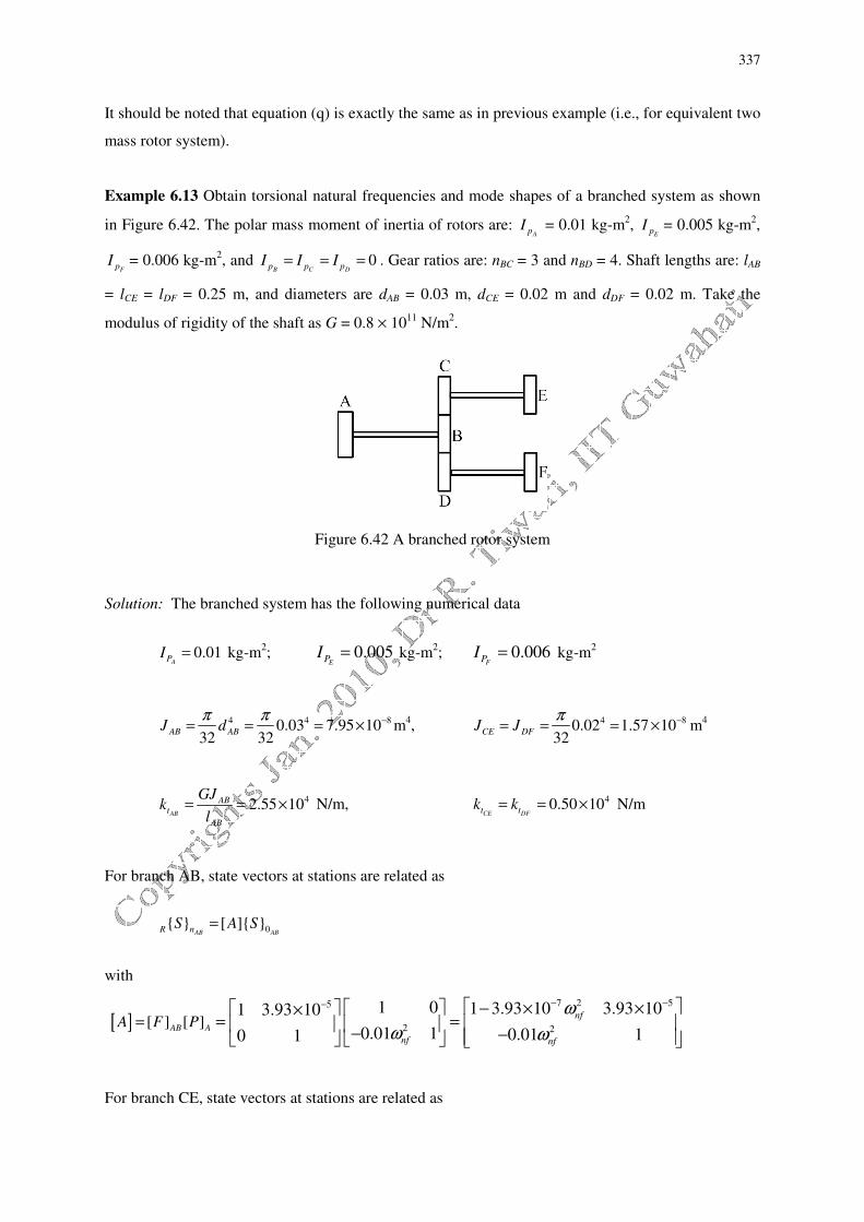
337

It should be noted that equation (q) is exactly the same as in previous example (i.e., for equivalent two

mass rotor system).

Example 6.13 Obtain torsional natural frequencies and mode shapes of a branched system as shown

in Figure 6.42. The polar mass moment of inertia of rotors are: ApI = 0.01 kg-m

2,

EpI = 0.005 kg-m2,

FpI = 0.006 kg-m2, and 0

B C Dp p pI I I= = = . Gear ratios are: nBC = 3 and nBD = 4. Shaft lengths are: lAB

= lCE = lDF = 0.25 m, and diameters are dAB = 0.03 m, dCE = 0.02 m and dDF = 0.02 m. Take the

modulus of rigidity of the shaft as G = 0.8 × 1011

N/m2.

Figure 6.42 A branched rotor system

Solution: The branched system has the following numerical data

0.01API = kg-m

2; 0.005

EPI = kg-m

2; 0.006

FPI = kg-m

2

4 4 80.03 7.95 1032 32

AB ABJ d

π π −= = = × m4, 4 80.02 1.57 10

32CE DF

J Jπ −= = = × m

4

42.55 10AB

AB

t

AB

GJk

l= = × N/m, 40.50 10

CE DFt tk k= = × N/m

For branch AB, state vectors at stations are related as

0{ } [ ]{ }AB ABR nS A S=

with

[ ] [ ] [ ]AB AA F P=

7 2 55

2 2

1 0 1 3.93 10 3.93 101 3.93 10

0.01 1 0.01 10 1

nf

nf nf

ω

ω ω

− −− − × × ×= = − −

For branch CE, state vectors at stations are related as

338

0{ } [ ]{ }CE CER n

S C S=

with

[ ]44

2 2 6 2

1 0 1 2.0 101 2.0 10[ ] [ ]

0.005 1 0.005 1 1.0 100 1E CE

nf nf nf

C P Fω ω ω

−−

−

× ×= = = − − − ×

Similarly, for branch DF, we have

0{ } [ ]{ }DF DFR n

S D S=

with

[ ]44

2 2 6 2

1 0 1 2.0 101 2.0 10[ ] [ ]

0.006 1 0.006 1 1.2 100 1F DF

nf nf nf

D P Fω ω ω

−−

−

× ×= = = − − − ×

From equation (6.81), the frequency equation can be written as

2 2 2 2

22 11 21 22 21 22 2211 21 0BC BD BC BD

a c d n a c d n a c d n n+ + =

On substitution, we get

( )( )( )7 2 6 2 21 3.93 10 1 1.0 10 0.006 9nf nf nf

ω ω ω− −− × − × − × +

( )( )( )7 2 2 6 21 3.93 10 0.005 1 1.2 10 16

nf nf nfω ω ω− −− × − − × × +

( )( )( )2 6 2 6 20.01 1 1.0 10 1 1.2 10 9 16 0

nf nf nfω ω ω− −− − × − × × × =

which can be simplified to

( )2 12 4 10 21.7685 10 3.3532 10 1.5740 0nf nf nf

ω ω ω− −× − × + =

Natural frequencies are given as

10nfω = ;

2924.4

nfω = rad/s and

31020.6

nfω = rad/s.

It can be seen that the rigid body mode exists since ends of the gear train is free. Mode shapes for

each of these natural frequencies can be obtained as follows.

339

For 01

=nfω with 0

1ABzϕ = as a reference value, angular displacements at various disc locations can

be written as

01

ABzϕ = ; 11 1nABz aϕ = = ;

0

11 10.33

3CEz

BC

a

nϕ = − = − − ;

0

12 2111

22

0.33nCE CEz z

c cc

cϕ ϕ

= − = −

;

0

11 10.25

4DFz

BD

a

nϕ = − = − = − ;

0

12 2111

22

0.25nDF DFz z

d dd

dϕ ϕ

= − = −

Figure 6.43 shows the mode shape. Similarly, for other natural frequencies displacements can be

obtained to get mode shapes as in Figures 6.44 and 6.45.

0 0.1 0.2 0.3 0.4 0.5-0.5

0

0.5

1

1.5

B

C E

A

D F

Position on discs and gears

Figure 6.43 Mode shape of the branched system for 1

0nfω =

Rel

ativ

e an

gula

r dis

pla

cem

ents

340

0 0.1 0.2 0.3 0.4 0.5-2

0

2

4

6

8

10

12

AB

F

EC,D

Position on discs and gears

Figure 6.44 Mode shape of the branched system for 2

924.4nfω = rad/s

0 0.1 0.2 0.3 0.4 0.5-1

0

1

2

3

4

5

6

AB

CD

E

F

Position on discs and gears

Figure 6.45 Mode shape of the branched system for 3

1020.6nfω = rad/s

Rel

ativ

e an

gula

r dis

pla

cem

ents

R

elat

ive

ang

ula

r dis

pla

cem

ents

341

6.8 TMM for Damped Torsional Vibrations

In any real rotor systems damping is always present. Torsional damping may come from several

sources, e.g. the shaft material, bearings, couplings, torsional vibration dampers, aerodynamic

damping at discs, rubbing of the rotor with the stator, loose components mounted on shaft, etc. The

shaft material or hysteretic damping comes due to intermolecular interaction in the shaft material,

which results in increase in the temperature of the shaft material. The torsional vibration damper is a

device which may be used to join together two-shaft section as shown in Fig. 6.46. It develops a

damping torque, which is dependent upon of the angular velocity on one shaft relative to the other.

These types of damping can be considered proportional to the relative angular velocity of discs to

which the shaft is connected and it is represented as cs. The disc aerodynamic (or rubbing) damping,

cd, comes due to interaction of the disc with the working fluid (like steam, gas, air, etc.), lubricant, and

coolant; which results in dissipation of the energy in the form of heat. This type of damping is

proportional to the angular velocity of the disc itself.

Figure 6.46 A schematic of a torsional vibration damper

Torsional dampers can be used as a means of attenuating (decreasing) system vibrations and to tune

system resonant frequencies to suit particular operating conditions. The damping in the system

introduces phase lag between the system displacement and torque.

Figure 6.47 General arrangement of multi-DOF rotor system with damping.

342

Figure 6.48 A free body diagram of rth rotor.

Figure 6.47 shows a general arrangement of torsional multi-DOF rotor system with the disc and the

shaft damping. From the free body diagram of nth rotor (Figure 6.48) the following governing

equations can be written as

n nL z R zϕ ϕ= (6.95)

and

n n n nd L z p L zR n L nT T c Iϕ ϕ− − =� �� (6.96)

For free vibration, torques RTn and LTn may be written in the form

j nf t

n nT T e

ω= (6.97)

where n

T is the complex amplitude of the torque at nth disc, and ωnf is the torsional natural frequency

of the system. The angular displacement takes the form

j nf

n n

t

z z eω

ϕ = Φ (6.98)

where nz

Φ is the complex amplitude of angular displacement at nth disc. Differentiating equations

(6.97) and (6.98) with respect to time and substituting in equations (6.95) and (6.96) leads to

2

1 0

+j 1nf p nf dR n L nnI cT Tω ω

Φ Φ = −

(6.99)

which can be simplified as

343

{ } [ ] { }L nR n n

S P S= (6.100)

with

[ ] 2

1 0

+j 1nf p nf d n

nP

I cω ω

= −

; { }L n

L n

ST

Φ =

where [P]n is a point matrix and [S]n is a state vector.

Figure 6.49 A free body diagram of nth shaft segment

The characteristics of the shaft element at station n (Fig. 6.49) are represented in the equation

describing the torque applied to the shaft at the location of rotor n, as

( ) ( )1 1n n n n nL n n L z R z s L z R z

T k cϕ ϕ ϕ ϕ− −

= − + −� � (6.101)

While the torque transmitted through the shaft is the same at both ends, i.e.,

1L n R nT T −= (6.102)

Substituting equations (6.97) and (6.98), in equations (6.101) and (6.102), we get

( ) ( )1 11 j

n n n n nR n n L z R z nf s L z R zT k cω

− −− = Φ − Φ + Φ − Φ (6.103)

and

1L n R nT T −= (6.104)

Combining equations (6.103) and (6.104), we get

1 1

j 0 j 1

0 1 0 1n

nf s nf s

L n n R n

k c k c

T T

ω ω

− −

+ Φ + Φ =

(6.105)

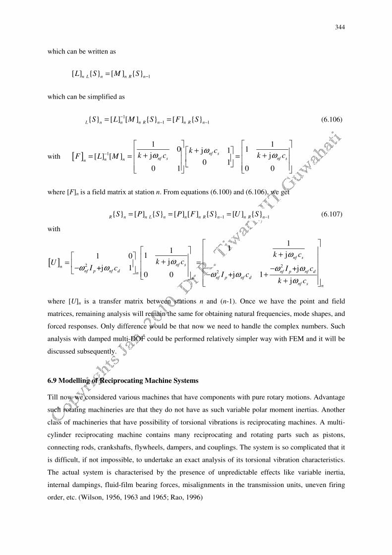
344

which can be written as

1[ ] { } [ ] { }n L n n R n

L S M S −=

which can be simplified as

1

1 1{ } [ ] [ ] { } [ ] { }L n n n R n n R n

S L M S F S−

− −= = (6.106)

with [ ] 1

1 10 1j 1

j j[ ] [ ]0 1

0 1 0 0

nf snf s nf sn nn

k ck c k cF L M

ωω ω−

+ + += = =

where [F]n is a field matrix at station n. From equations (6.100) and (6.106), we get

1 1{ } [ ] { } [ ] [ ] { } [ ] { }R n n L n n n R n n R n

S P S P F S U S− −= = = (6.107)

with

[ ] 2 2

2

111

j11 0j

+j 1 +j+j 10 0

j

nf s

nf snnf p nf d nf p nf dn

nf p nf dn

nf s n

k ck cU

I c I cI c

k c

ωω

ω ω ω ωω ω

ω

+ += = − − − +

+

where [U]n is a transfer matrix between stations n and (n-1). Once we have the point and field

matrices, remaining analysis will remain the same for obtaining natural frequencies, mode shapes, and

forced responses. Only difference would be that now we need to handle the complex numbers. Such

analysis with damped multi-DOF could be performed relatively simpler way with FEM and it will be

discussed subsequently.

6.9 Modelling of Reciprocating Machine Systems

Till now we considered various machines that have components with pure rotary motions. Advantage

such rotating machineries are that they do not have as such variable polar moment inertias. Another

class of machineries that have possibility of torsional vibrations is reciprocating machines. A multi-

cylinder reciprocating machine contains many reciprocating and rotating parts such as pistons,

connecting rods, crankshafts, flywheels, dampers, and couplings. The system is so complicated that it

is difficult, if not impossible, to undertake an exact analysis of its torsional vibration characteristics.

The actual system is characterised by the presence of unpredictable effects like variable inertia,

internal dampings, fluid-film bearing forces, misalignments in the transmission units, uneven firing

order, etc. (Wilson, 1956, 1963 and 1965; Rao, 1996)

345

The analysis can be best carried out, by lumping the inertias of rotating and reciprocating parts at

discrete points on the main shaft. The problem then reduces to the forced torsional vibration study of

an multi-DOF rotor system subjected to varying torques at different cylinder points. The crankshaft

and the other drive or driven shafts are generally flexible in torsion, but have low polar moments of

inertia, unlike in the case of some large turbines or compressors. On the other hand, parts mounted on

the shafting, like the damper, flywheel, generator etc. are rigid and will have very high polar moments

of inertia. The system containing the crankshaft, coupling, generator, auxiliary drive shaft, other

driven shaft like pumps, and mounted parts can then be reduced to a simple system with a series of

rigid rotor (representing the inertias) connected by the massless flexible shafts as shown in Figure

6.50. Now simple procedures will be described to reduce reciprocating inertias to equivalent rotating

inertias, the uneven crack shaft geometry to an equivalent uniform shaft system, and the conversion of

periodic torque variation to its components.

Figure 6.50 A rotor model with N-disc of a typical reciprocating engine installation

6.9.1 An equivalent polar mass moment of inertia

Determination of a polar mass moment of inertia is a straightforward matter for rotating parts,

however, it is not quite so simple in the case of reciprocating parts. Consider the piston shown in two

different positions in Figure 6.51 and let us imagine the crankshaft with a polar mass moment of

inertia, mrev r2

, where mrev is the total revolving mass at the crack radius r (it is also called crack

through). It includes all the revolving part of the crankcr

m , and the only the revolving part of the

connecting rod rev

cnm (when its two mass equivalent dynamic system is considered). Let us assume that

the crack is not revolving, however, it is executing small torsional oscillations about the mean position

shown in diagrams.

346

In first case (Fig. 6.51a) there is no motion for the piston, with small oscillations of the crank and

hence the equivalent polar mass moment of inertia of the piston is zero. Whereas in second case (Fig.

6.51(b)), the piston has practically the same acceleration as that of the crank pin and the equivalent

polar moment inertia is mrec r2, where mrec is the mass of the reciprocating parts. It includes all the

mass of the piston mp, and only the reciprocating part of the connecting rod rec

cnm when it is converted

to a two-mass equivalent dynamic system. Hence, the total polar mass moment of inertia varies from

mrev r2 to (mrev r

2 + mrec r

2), when the crankshaft is rotating.

The inertia of connecting rod can be obtained by considering a two-mass equivalent dynamic system

with mass one at piston, rec

cnm , and other mass at crank pin, rev

cnm . With some approximation (for more

accuracy refer to Bevan, 1984) the mass of the connecting rod cn

m can be considered as two mass

system one at the piston of magnitude /rec

cn cnm m a l= , and another at the crack radius of magnitude

/rev

cn cnm m c l= , where l is the length of the connecting rod, c is the distance from the piston pin to the

center of gravity of the connecting rod, and a is the distance from the crack pin to the center of gravity

of the connecting rod (i.e., l = a + c). It will contribute to both mrev and mrec by small amount. We

consider as an approximation in the system to have an average inertia given by

2 20.5p rev recI m r m r= + (6.108)

with

rev

rev cr cnm m m= + and rec

rec p cnm m m= + (6.109)

where r is crank radius.

Figure 6.51 An equivalent mass moment of inertia of the piston and the connecting rod

347

6.9.2 Equivalent torsional stiffness of crack shafts

In determining the torsional stiffness of shafts connecting rotors, the main difficulty arises from the

crank webs. Considering a crank shaft into an equivalent ordinary shaft having the same flexibility as

the original one, as shown in Figure 6.52. Through this idealisation is physically possible, but the

calculations involved are extremely difficult. This is because the crank webs are subjected to bending

and the crank pin to twisting, when the main shaft is subjected to twisting. Moreover, the beam

formulae, if used will not very accurate, because of short stubs involved rather than long beams

usually considered. Further torques applied at the free end also give rise to sidewise displacement, i.e.

coupled beading-torsion exists; which is prevented in the machine. For high-speed lightweight

engines, the crank webs are no more rectangular blocks and application of the theory becomes

extremely difficult. Because of this uncertainties in analytical calculation to estimate the torsional

stiffness of crank throws, several experiments have been carried out on a number of crank shafts of

large slow speed engines, which have shown that the equivalent length le is nearly equal to the actual

length, if the diameter of main shaft is equal to the crank pin diameter.

Figure 6.52 Equivalent length of a crank

In general the procedure that is applied to reduce the reciprocating machine system to a mathematical

model, is to use a basic diameter, which corresponding to the journal diameter of the crankshaft. The

torsional stiffness is all calculated based on the basic diameter, irrespective of their actual diameter.

For the end rotors (i.e., the generator rotor) compute the stiffness of the shaft from the coupling up to

the point of rigidity. In case where one part of the system is connected to the other part through gears,

or other transmission units, it is convenient to reduce all the inertias and stiffness to one reference

speed. Finite element methods can be used to obtain equivalent stiffness of the crackshafts. Once the

mathematical model is developed, it can be used in illustrating the critical speed calculations, and

forced vibration responses.

348

6.9.3 Torque variations in a reciprocating machinery

Torsional oscillation in the crankshaft and in the shafting of driven machinery is vibration

phenomenon of practical importance in the design of reciprocating engines. The average torque

delivered by a cylinder in a reciprocating machine, is a small fraction of the maximum torque, which

occurs during the firing period. Even though the torque is periodic the fact that it fluctuates so

violently within the period, constitutes one of the inherent disadvantages of a reciprocating machine,

from the dynamics point of view, as compared with a turbine where the torque is practically uniform.

It is possible to express the torque by a reciprocating engine into its harmonic components of several

orders of the engine speed, and these harmonic components can excite the engine driven installations

into forced torsional vibrations. The engine and the driven unit such as generator or a pump are

normally connected by a flexible coupling and thus the total installation has fairly low natural

frequencies falling in the speed range of the engine and the harmonics of different order. It is a

commonly known fact that failures can occur in reciprocating machine installations, when the running

speed of the engine is at or near a dominant torsional critical speed of the system. High dynamic

stresses can occur in the main shafting of such engine installations and to avoid these conditions, it is

essential that the torsional vibration characteristics of the entire installation be analysed before the

unit is put into operation. Any analysis of torsional vibration characteristics of reciprocating

machinery should finally predict the maximum dynamic stresses or torque developed in the shafting

and couplings of the system, as accurately as possible, so that they can be compared with the

permissible values, to check the safety of installation.

Example 6.14 A marine reciprocating engine, flywheel and propeller are approximately equivalent to

the following three-rotor system. The engine has a crack 50 cm long and a connecting rod 250 cm

long. The engine revolving parts are equivalent to 50 kg at crank radius, and the piston and pin masses

are 41 kg. The connecting rod mass is 52 kg and its center of gravity is 26 cm from the crankpin

center. The mass of the flywheel is 200 kg with the radius of gyration of 25 cm. The propeller has the

polar mass moment of inertia of 6 kg-m2. The equivalent shaft between the engine masses and the

flywheel is 38 cm diameter and 5.3 m long and that between the flywheel and the propeller is 36 cm

diameter and 1.5 m long. Find the natural frequencies of the torsional vibrations of the system.

Solution: The main aim of the present solution procedure would be to first find the equivalent rotating

mass of the reciprocating engine, once it has been done then the problem will reduce to obtaining the

natural frequencies of a three-rotor system as shown in Figure 6.53. The three revolving masses are

corresponding to the reciprocating engine, flywheel, and propeller.

349

Figure 6.53 A three-disc model of the engine, flywheel and propeller

The equivalent rotating part of the engine can be obtained as follows. We have the following engine

data:

Crank radius, r = 0.5 m, Mass of crank revolving parts, mcr = 50 kg at the crank radius

Length of connecting rod l = 2.5 m, Mass of the connecting rod, mcn = 52 kg,

Distance of center of gravity of the connecting rod from the crack pin, a = 0.26 m

Distance of center of gravity of the connecting rod from the piston pin, c = 2.24 m

Piston and pin masses, mp = 41 kg

Hence, the equivalent (approximate) reciprocating and revolving masses of the connecting rod would

be

/ 52 0.26 / 2.5 5.41rec

cn cnm m a l= = × = kg; / 52 2.24 / 2.5 46.59rev

cn cnm m c l= = × = kg

The equivalent revolving and reciprocating masses are given as

50 46.59 96.59rev

rev cr cnm m m= + = + = kg

and

41 5.41 46.41rec

rec p cnm m m= + = + = kg

Hence, the equivalent polar mass moment of inertia of the engine is obtained as

2 2) (96.59 0.5 46.41) 0.5 29.95( 0.5

ep rev recI m m r+ = + × × == kg-m2

Now, the polar mass moment of inertia of the flywheel ( )22 200 0.25 12.5

fp fI mr= = × = kg-m

2

For the propeller, the polar mass moment of inertia is given as 6ppI = kg-m

2.

350

The torsional stiffness of shaft segments (1) and (2) are given as

1

9 471 1

1

78.9 10 0.383 10

32 5.3t

G Jk

l

π× × ×= = = ×

×N-m/rad

and

2

9 472 2

2

78.9 10 0.368.67 10

32 1.5t

G Jk

l

π× × ×= = = ×

×N-m/rad

Natural frequencies of three-disc rotor system (with 1ep pI I= ,

2fp pI I= and 3pp pI I= ) are given as

(equation (6.110))

10nfω =

and

( )1 2 1 2 32 3 2 31 2 1 2

2,3 1 2 1 2

1 2 2 3 1 2 2 3 1 2 3

2

2 1 1

2 4

t t p p pp p p pp p p p

nf t t t t

p p p p p p p p p p p

k k I I II I I II I I Ik k k k

I I I I I I I I I I Iω

+ + + ++ + = + ± + −

which gives

10nfω =

2

31.58 10nfω = × rad/s 3

34.72 10nfω = × rad/s

Finding of mode shapes and the position of nodes is left to the reader as a practice problem.

351

Concluding remarks

To summarise, now we have clear idea about torsional natural frequencies and mode shapes for

simple rotor systems. We have obtained torsional natural frequencies and mode shapes using

Newton’s second law of motion, and using the systematic transfer matrix method (TMM). The TMM

is found to be quite versatile and easy in application especially for the multi-DOF rotor systems. The

TMM is also developed for rotor system with damping in the disc due to aerodynamic forces and in

the shaft due to material damping (both the damping models are taken as viscous damping). Apart

form these simple rotor systems, we considered the geared and branched systems for obtaining

torsional natural frequencies. For the multi-DOF geared and branched systems, the TMM is applied

because of its simplicity in the application. At the end the procedure of obtaining the equivalent rotor

system from multi-cylinder reciprocating engines is briefly discussed and for detailed analysis a brief

literature review is given.

352

Exercise Problems

Exercise 6.1 Find torsional natural frequencies and mode shapes of the two-disc rotor system shown

in Figure E6.1 by using the transfer matrix method. B1 and B2 are frictionless bearings, and D1 and D2

are rigid discs. The shaft is made of steel with the modulus of rigidity G = 0.8(10)11

N/m2, and a

uniform diameter d = 10 mm. Various shaft lengths are as follows: B1D1 = 50 mm, D1D2 = 75 mm,

and D2B2 = 50 mm. The polar mass moment of inertia of discs is: 1pI = 0.0008 kg-m2 and

2pI = 0.002

kg-m2. Consider the shaft as massless. [Answer:

10nfω = ,

21354nfω = rad/s]

Figure E6.1

Exercise 6.2 Obtain the torsional natural frequency of an overhung rotor system as shown in Figure

E6.2. The end B1 of the shaft has a fixed end condition. The shaft diameter is 10 mm, and total length

of the shaft is 0.2 m. The polar mass moment of inertia equal to 0.02 kg-m2. Neglect the mass of the

shaft. Use the transfer matrix method.

Figure E6.2

Exercise 6.3 Find the torsional natural frequencies and mode shapes of a rotor system as shown in

Figure E6.3 by using the transfer matrix method. B1 and B2 are fixed supports, and D1 and D2 are rigid

discs. The shaft is made of steel with the modulus of rigidity of G = 0.8 (10)11

N/m2 and has uniform

diameter of d = 10 mm. Different shaft lengths are as follows: B1D1 = 50 mm, D1D2 = 75 mm, and

D2B2 = 50 mm. The polar mass moment of inertia of discs is: 1pI = 0.08 kg-m

2 and

2pI = 0.2 kg-m2.

Consider the shaft as massless. [Answer: 1nfω = 100.29 rad/s, {

zϕ }1 = {1 1.73}

T;

2nfω = 189.05 rad/s,

{z

ϕ }2 = {1 1/4.33}T]

353

Figure E6.3

Exercise 6.4 Find all torsional natural frequencies and draw corresponding mode shapes of the rotor

system shown in Figure E6.4. B1 is fixed supported (with zero angular displacement about shaft axis)

and B2 and B3 are simply supported (with non-zero angular displacements). The shaft is made of steel

with G = 0.8×1011

N/m2, and uniform diameter d = 10mm. The various shaft lengths are as follows:

1 150mmB D = ;

1 250mmD B = ;

2 225mmB D = ;

2 325mmD B = ;

3 330mmB D = . The polar mass

moment of inertia of discs is: 1

0.002pI = kg-m2;

20.001pI = kg-m

2, and

30.008pI = kg-m

2; Use the

transfer matrix method. Give all detailed steps involved in obtaining the final system of equation and

application of boundary conditions. Consider the shaft as mass-less and discs are lumped masses.

[Answer: 1 2 3

518.1Hz, 1184.6Hz, 1977Hznf nf nfω ω ω= = =

1

0

1

2

3

0

1

1.984

2.344nf

z

z

z

z ω

ϕ

ϕ

ϕ

ϕ

=

,

2

0

1

2

3

0

1.000

1.791

0.835nf

z

z

z

z ω

ϕ

ϕ

ϕ

ϕ

= −

−

,

3

0

1

2

3

0

1.000

2.95

2.49nf

z

z

z

z ω

ϕ

ϕ

ϕ

ϕ

= −

]

Figure E6.4 A multi-support multi-disc rotor system

Exercise 6.5 Obtain torsional natural frequencies of a turbine-coupling-generator rotor system as

shown in Figure E6.5 by the transfer matrix method. The rotor is assumed to be supported on

frictionless bearings. The polar mass moment of inertia of the turbine, coupling and generator is Tp

I =

25 kg-m2,

CpI = 5 kg-m

2 and

GpI = 50 kg-m

2, respectively. Take the modulus of rigidity of the shaft as

G = 0.8 × 1011

N/m2. Assume the shaft diameter throughout equal to 0.2 m, and lengths of shafts

between the bearing-turbine-coupling-generator-bearing are 1 m each so that the total span is 4 m. The

coupling also gives a point flexibility (inverse of stiffness) equivalent to 5 times that of a shaft with 1

m of length and 0.2m of diameter. Consider the shaft as massless.

354

Figure E6.5 A turbine-generator set

Exercise 6.6 Obtain the torsional natural frequency of an overhung rotor system as shown in Figure

E6.6 Take the polar mass moment of inertia of the disc as, Ip = 0.04 kg-m2. The massless shaft has

following properties: lengths are a = 0.3 m, b = 0.7 m, the uniform diameter is 10 mm, and the

modulus of rigidity G = 0.8 × 1011

N/m2. Bearing ‘A’ is flexible and provides a torsional restoring

toque with its torsional stiffness equal to 5 percent of the torsional stiffness of the shaft segment

having length a. Consider bearing B is a fixed bearing. Use both the direct and transfer matrix

methods. [Hint: We need to find the effective torsional stiffness of the rotor system].

Figure E6.6 An overhung rotor system with an intermediate support

Exercise 6.7 A small electric motor drives another through a long coil spring (n turns, wire diameter

d, coil diameter D). The two motor rotors have inertias p

I1 and

pI

2. Calculate torsional natural

frequencies of the set-up. Assuming the ends of the spring to be “built-in” to the shafts. [Hint:

Consider the system as a two-mass rotor system and the stiffness of a spring is given as

4

38t

Gdk

D n= , Answer:

10nfω = and

( )1 2

2

1 2

t p p

nf

p p

k I I

I Iω

+= ].

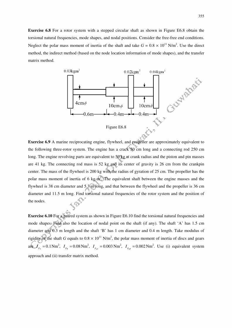
355

Exercise 6.8 For a rotor system with a stepped circular shaft as shown in Figure E6.8 obtain the

torsional natural frequencies, mode shapes, and nodal positions. Consider the free-free end conditions.

Neglect the polar mass moment of inertia of the shaft and take G = 0.8 × 1011

N/m2. Use the direct

method, the indirect method (based on the node location information of mode shapes), and the transfer

matrix method.

Figure E6.8

Exercise 6.9 A marine reciprocating engine, flywheel, and propeller are approximately equivalent to

the following three-rotor system. The engine has a crack 50 cm long and a connecting rod 250 cm

long. The engine revolving parts are equivalent to 50 kg at crank radius and the piston and pin masses

are 41 kg. The connecting rod mass is 52 kg and its center of gravity is 26 cm from the crankpin

center. The mass of the flywheel is 200 kg with the radius of gyration of 25 cm. The propeller has the

polar mass moment of inertia of 6 kg-m2. The equivalent shaft between the engine masses and the

flywheel is 38 cm diameter and 5.3 m long, and that between the flywheel and the propeller is 36 cm

diameter and 11.5 m long. Find torsional natural frequencies of the rotor system and the position of

the nodes.

Exercise 6.10 For a geared system as shown in Figure E6.10 find the torsional natural frequencies and

mode shapes. Find also the location of nodal point on the shaft (if any). The shaft ‘A’ has 1.5 cm

diameter and 0.3 m length and the shaft ‘B’ has 1 cm diameter and 0.4 m length. Take modulus of

rigidity of the shaft G equals to 0.8 × 1011

N/m2, the polar mass moment of inertia of discs and gears

are 0.1ApI = Nm

2, 0.08

BpI = Nm2, 0.003

gApI = Nm2, 0.002

gBpI = Nm2. Use (i) equivalent system

approach and (ii) transfer matrix method.

356

Figure E6.10 A geared rotor system

Exercise 6.11 Obtain torsional natural frequencies and mode shapes of an epi-cyclic gear train as

shown in Figure E6.11. Find also the location of nodal point on the shaft. The gear mounted on shaft

‘B’ is a planetary gear and the gear on shaft ‘A’ is a sun gear. Consider the polar mass moment of

inertia of the shaft, the arm and gears as negligible. Shaft ‘A’ has 5 cm of diameter and 0.75 m of

length and shaft ‘B’ has 4 cm of diameter and 1.0 m of length. Angular speeds of shaft A and the arm

are 300 rpm and 100 rpm, respectively. Take the modulus of rigidity of the shaft G equals to 0.8 ×

1011

N/m2, the polar mass moment of inertia of discs are

ApI = 24 Nm2 and

BpI = 10 Nm2. State the

assumptions made in the analysis. [nAB = 1, 1

0nfω = , {u}1 = {1 1 -1}T;

253.34nfω = rad/s, {u}2 = {1

0.04 3.37}T; node location from left hand side x = 0.72 m].

Figure E6.11 An epi-cyclic geared system

Exercise 6.12 For a gear train as shown in Figure E6.12, obtain torsional natural frequencies and the

location of the node. Dimensions of shafts are as follows (i) motor shaft: 0.20 m length and 0.015 m

diameter, (ii) flywheel shaft: 0.2 m of length and 0.01 m of diameter, and (iii) intermediate shaft: 0.4

m of length and 0.012 m of diameter. The polar mass moment of inertia of the motor and flywheel are

357

Flywheel

Motor

0.01mpI = kg-m

2 and 0.04

mpI = kg-m2, respectively. Gear ratio of the first and second gear pairs are 3

and 4, respectively. Neglect inertias of gears and mass of shafts. Assume the free-free end conditions

and all shafts are mounted on frictionless bearings. Take G = 0.8×1011

N/m2. Use the TMM.

Figure E6.12

Exercise 6.13 A stepped-shaft consists of three segments with lengths of 40 cm, 30 cm and 40 cm;

and corresponding diameters as, d cm, 13 cm and d cm, where d is an unknown. The shaft has two

flywheels (1

11pI = kg-m2 and

211pI = kg-m

2, with radius of gyration of both flywheel equals to 0.5

m) at the ends, and the shaft is supported on two frictionless rolling bearings at 20 cm away from the

either ends. The operating speed of the shaft is 1500 rpm and due to rotation of the shaft it has

external torque impulses such that it has period corresponding to the quarter of the shaft rotation.

Obtain the diameter, d, such that the torsional critical speed may be 20% above the external torque

frequency (fundamental harmonics). Obtain the transverse natural frequency of rotor system, so

designed based on the dynamics of the rotor in torsion. Neglect the mass of the shaft, and take G =

0.8×1011

N/m2, and E = 2.1×10

11 N/m

2.

Exercise 6.14 A motor has rotating masses of the polar mass moment of inertia of 58 kg-m2, which is

connected to one end of a shaft of 6 cm diameter and 2.30 m long. At the other end a flywheel and

pinion are attached, with the effective polar mass moment of inertia of 220 kg-m2. The pinion is

connected to a gear with a gear ratio of 4 and of the polar mass moment of inertia of 70 kg-m2, which

drives a pump. The measured torsional vibration frequency of the rotor system is 60 Hz. Find the

effective polar mass moment of inertia of the pump impeller and entrained water. Take G = 0.8×1011

N/m2.

Exercise 6.15 A cantilever shaft of 1 m length (l), and 30 mm diameter (d) has a thin disc of 5 kg

mass (m) attached at its free end, with the disc radius of 5 cm. The shaft has a through hole parallel to

the shaft axis of diameter 3 mm (di), which is vertically below the shaft center, with the distance

358

between the centres of the shaft and the hole as 6 mm (e). Consider no warping of the plane; and

obtain the torsional natural frequencies of the shaft system. Consider the shaft as massless and

modulus of rigidity G = 0.8× 1011

N/m2. [Hint: Find the equivalent stiffness of the shaft and then

obtain natural frequencies: /eqnf t p

k Iω = eqt

GJk

l= , ( )4 4 2 2 8

1 2 8 7.926 1032

i iJ I I d d d e

π −= + = − − = ×

m4; 1007.23nfω = rad/s]

Exercise 6.16 Find torsional natural frequencies and mode shapes of the rotor system shown in Figure

E6.16. B is a fixed bearing, which provide fixed support end condition; and D1, D2, D3 and D4 are

rigid discs. The shaft is made of the steel with the modulus of rigidity G = 0.8 (10)11

N/m2 and the

uniform diameter d = 20 mm. Various shaft lengths are as follows: D1D2 = 50 mm, D2D3 = 50 mm,

D3D4 = 50 mm and D4B2 = 150 mm. The mass of discs are: m1 = 4 kg, m2 = 5 kg, m3 = 6 kg and m4 = 7

kg. Consider the shaft as mass-less. Consider discs as thin and take diameter of discs as d =1

12 cm,

d =2

6 cm, and d =

312 cm, d =

414 cm.

Figure E6.16 A multi-disc overhung rotor

Exercise 6.17 Find torsional natural frequencies and mode shapes of the rotor system shown in Figure

E6.17. B is a fixed bearing, which provide fixed support end condition; and D1, D2, D3, D4 and D5 are

rigid discs. The shaft is made of the steel with the modulus of rigidity G = 0.8 (10)11

N/m2 and the

uniform diameter d = 20 mm. Various shaft lengths are as follows: D1D2 = 50 mm, D2D3 = 50 mm,

D3D4 = 50 mm, D4D5 = 50 mm, and D5B2 = 50 mm. The mass of discs are: m1 = 4 kg, m2 = 5 kg, m3 =

6 kg, m4 = 7 kg, and m4 = 8 kg. Consider the shaft as massless. Tow cases to be considered (i)

Consider the disc as point masses, i.e., neglect the diametral and polar mass moment of inertia of all

discs; (ii) consider discs as thin and take diameter of discs as d =1

12 cm, d =2

6 cm, and d =

312 cm,

d =4

14 cm, and d =5

16 , however, neglect the gyroscopic effects.

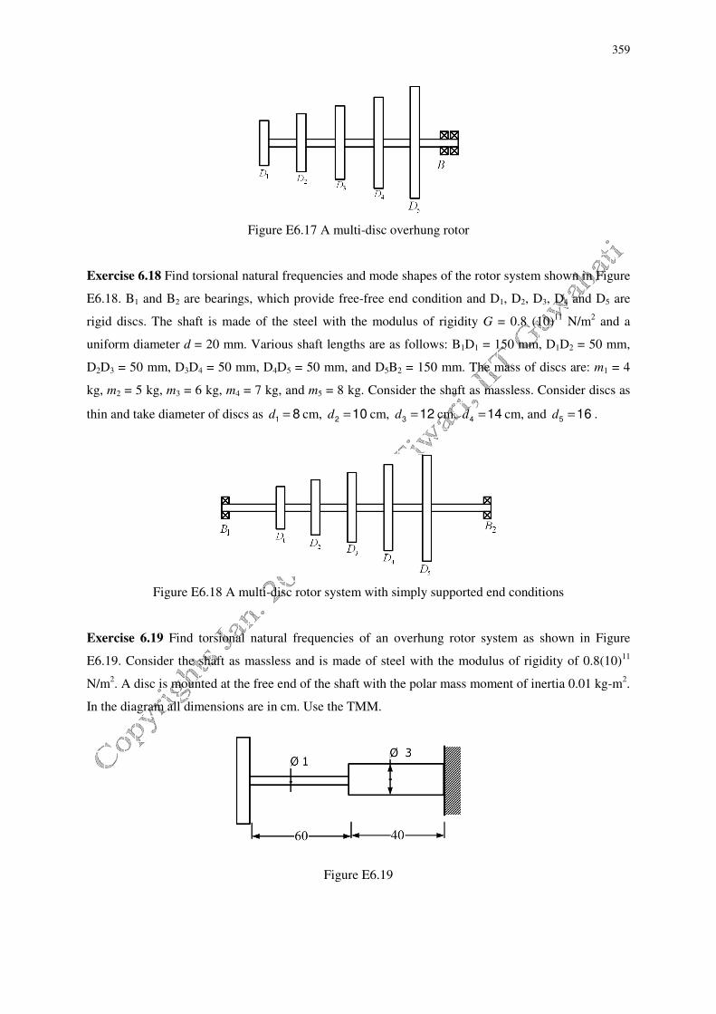
359

Figure E6.17 A multi-disc overhung rotor

Exercise 6.18 Find torsional natural frequencies and mode shapes of the rotor system shown in Figure

E6.18. B1 and B2 are bearings, which provide free-free end condition and D1, D2, D3, D4 and D5 are

rigid discs. The shaft is made of the steel with the modulus of rigidity G = 0.8 (10)11

N/m2 and a

uniform diameter d = 20 mm. Various shaft lengths are as follows: B1D1 = 150 mm, D1D2 = 50 mm,

D2D3 = 50 mm, D3D4 = 50 mm, D4D5 = 50 mm, and D5B2 = 150 mm. The mass of discs are: m1 = 4

kg, m2 = 5 kg, m3 = 6 kg, m4 = 7 kg, and m5 = 8 kg. Consider the shaft as massless. Consider discs as

thin and take diameter of discs as d =1

8 cm, d =2

10 cm, d =

312 cm, d =

414 cm, and d =

516 .

Figure E6.18 A multi-disc rotor system with simply supported end conditions

Exercise 6.19 Find torsional natural frequencies of an overhung rotor system as shown in Figure

E6.19. Consider the shaft as massless and is made of steel with the modulus of rigidity of 0.8(10)11

N/m2. A disc is mounted at the free end of the shaft with the polar mass moment of inertia 0.01 kg-m

2.

In the diagram all dimensions are in cm. Use the TMM.

Figure E6.19

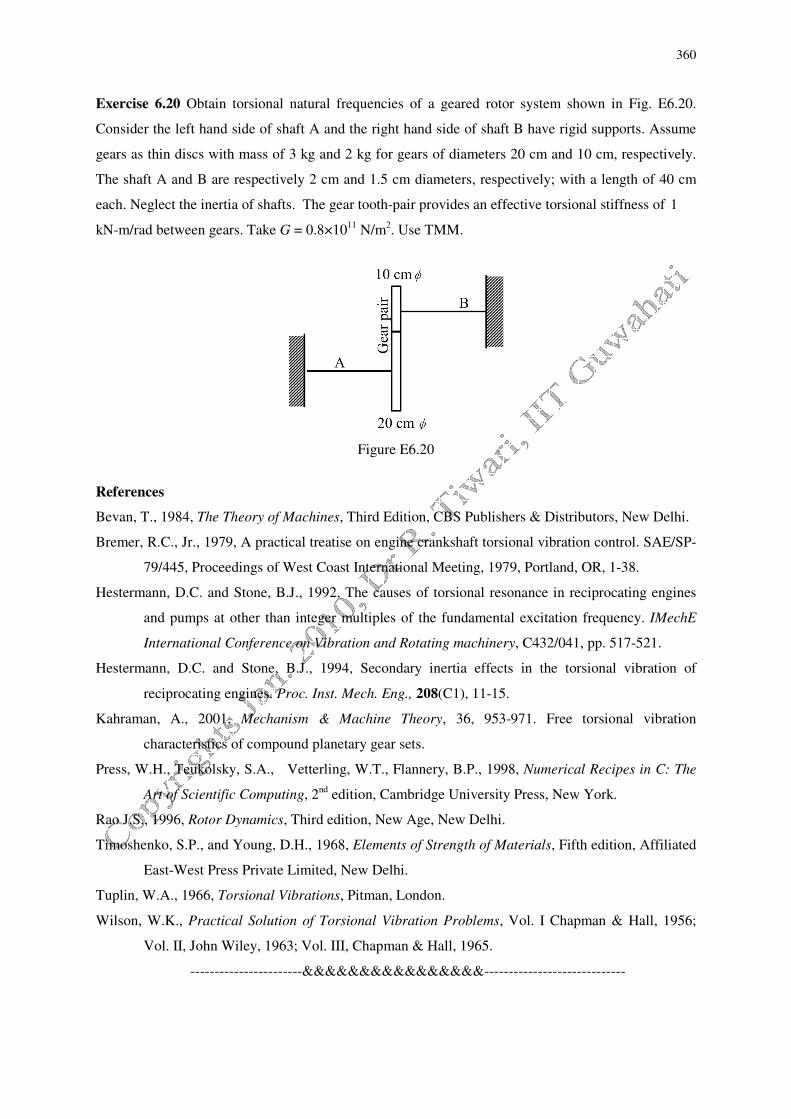
360

Exercise 6.20 Obtain torsional natural frequencies of a geared rotor system shown in Fig. E6.20.

Consider the left hand side of shaft A and the right hand side of shaft B have rigid supports. Assume

gears as thin discs with mass of 3 kg and 2 kg for gears of diameters 20 cm and 10 cm, respectively.

The shaft A and B are respectively 2 cm and 1.5 cm diameters, respectively; with a length of 40 cm

each. Neglect the inertia of shafts. The gear tooth-pair provides an effective torsional stiffness of 1

kN-m/rad between gears. Take G = 0.8×1011

N/m2. Use TMM.

Figure E6.20

References

Bevan, T., 1984, The Theory of Machines, Third Edition, CBS Publishers & Distributors, New Delhi.

Bremer, R.C., Jr., 1979, A practical treatise on engine crankshaft torsional vibration control. SAE/SP-

79/445, Proceedings of West Coast International Meeting, 1979, Portland, OR, 1-38.

Hestermann, D.C. and Stone, B.J., 1992, The causes of torsional resonance in reciprocating engines

and pumps at other than integer multiples of the fundamental excitation frequency. IMechE

International Conference on Vibration and Rotating machinery, C432/041, pp. 517-521.

Hestermann, D.C. and Stone, B.J., 1994, Secondary inertia effects in the torsional vibration of

reciprocating engines. Proc. Inst. Mech. Eng., 208(C1), 11-15.

Kahraman, A., 2001, Mechanism & Machine Theory, 36, 953-971. Free torsional vibration

characteristics of compound planetary gear sets.

Press, W.H., Teukolsky, S.A., Vetterling, W.T., Flannery, B.P., 1998, Numerical Recipes in C: The

Art of Scientific Computing, 2nd

edition, Cambridge University Press, New York.

Rao J.S., 1996, Rotor Dynamics, Third edition, New Age, New Delhi.

Timoshenko, S.P., and Young, D.H., 1968, Elements of Strength of Materials, Fifth edition, Affiliated

East-West Press Private Limited, New Delhi.

Tuplin, W.A., 1966, Torsional Vibrations, Pitman, London.

Wilson, W.K., Practical Solution of Torsional Vibration Problems, Vol. I Chapman & Hall, 1956;

Vol. II, John Wiley, 1963; Vol. III, Chapman & Hall, 1965.

-----------------------&&&&&&&&&&&&&&&&-----------------------------