chapter 8 a statistics primer winston jackson and norine verberg methods: doing social research, 4e
TRANSCRIPT

Chapter 8A Statistics Primer
Winston Jackson and Norine Verberg
Methods: Doing Social Research, 4e
8-2© 2007 Pearson Education Canada
Level of Measurement
Measures can be designed to have a higher, more complex level or a more basic, rudimentary level Influenced by how the variable is conceptualized Gender: can have only two categories (males and
females) Age: can be age (year of birth) or age groups (age
categories, e.g., adolescent, young adult, etc.) Influences choice of statistical analysis
Shown on Table 8.11 on page 222 Related to measurement error (Chapter 13)

8-3© 2007 Pearson Education Canada
Three Levels of Measurement
Nominal: involves no underlying continuum; assignment of numeric values arbitrary Examples: religious affiliation, gender, etc
Ordinal: implies an underlying continuum; values are ordered but intervals are not equal. Examples: community size, Likert items, etc.
Ratio: involves an underlying continuum; numeric values assigned reflect equal intervals; zero point aligned with true zero. Examples: weight, age in years, % minority
8-4© 2007 Pearson Education Canada
Examples of Nominal Level Measures
Do you have a valid driver’s licence? [ ] Yes
[ ] No
Your sex (Circle number of your answer)
1 Male
2 Female
8-5© 2007 Pearson Education Canada
Example of Ordinal Level Measure
The population of the place I considered my hometown when growing up was:
Rural area 1town under 5,000 25,000 to 19,999 320,000 to 99,999 4100,000 to 999,999 51,000,000 or over 6
8-6© 2007 Pearson Education Canada
Examples of Ratio Level Measures
In the following items, circle a number to indicate the extent to which you agree or disagree with each statement. I would quit my present job if I won $1,000,000 through a lottery. Strongly Disagree 1 2 3 4 5 6 7 8 9 Strongly Agree I would be satisfied if my child followed the same type of career as I have. Strongly Somewhat Neither Agree Somewhat StronglyDisagree Disagree nor Disagree Agree Agree 1 2 3 4 5

8-7© 2007 Pearson Education Canada
Describing an Individual Variable
Statistics provide ways to describe and compare sets of observations (e.g., income levels, infant mortality, morbidity, crime, etc.)
Two common ways of describing a distribution (a set of scores in a data set) Measures of central tendency Measures of dispersion

8-8© 2007 Pearson Education Canada
Measures of Central Tendency
A number that typifies the central scores of a set of values Mean Median Mode
8-9© 2007 Pearson Education Canada
Mean
The arithmetic average or average Calculated by summing values and dividing by
number of cases Used to describe central tendency of ratio level
data

8-10© 2007 Pearson Education Canada
Median
The midpoint Used to describe central tendency of ordinal
level data Calculated by ordering a set of values and
then using the middlemost value (in cases of two middle values, calculate the mean of the two values).
Often used when a data set has extreme cases

8-11© 2007 Pearson Education Canada
Table 8.7 Median for Extreme ValuesCASE # $ INCOME
1. 5,400
2. 6,600
3. 7,700
4. 10,200
5. 13,400
6. 16,400
7. 16,700
8. 18,300 ← $18,300 median value
9. 19,000
10. 20,000
11. 20,500
12. 22,900
13. 24,600
14. 31,500 $54,213 mean value
15. 580,000

8-12© 2007 Pearson Education Canada
Mode
The most frequently occurring value Used to describe central tendency of nominal level
data (gender, religion, nationality)
TABLE 8.8 DISTRIBUTION OF RESPONDENTS BY COUNTRY
COUNTRY NUMBER PERCENT
Canada 65 34.9 ← mode
New Zealand 58 31.2
Australia 63 33.9
TOTAL 186 100.0

8-13© 2007 Pearson Education Canada
Measures of Dispersion
Indicates dispersion or variability of values Are scores close together or spread out?
Three common measures of dispersion: Range Standard deviation Variance
8-14© 2007 Pearson Education Canada
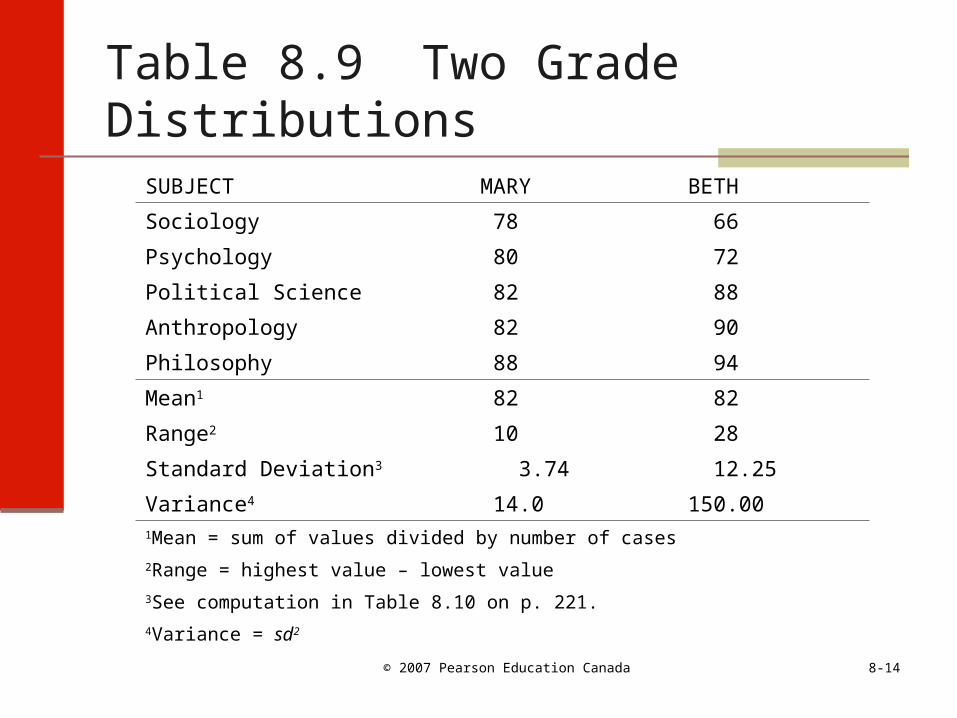
Table 8.9 Two Grade Distributions
SUBJECT MARY BETH
Sociology 78 66
Psychology 80 72
Political Science 82 88
Anthropology 82 90
Philosophy 88 94
Mean1 82 82
Range2 10 28
Standard Deviation3 3.74 12.25
Variance4 14.0 150.001Mean = sum of values divided by number of cases
2Range = highest value – lowest value
3See computation in Table 8.10 on p. 221.
4Variance = sd2

8-15© 2007 Pearson Education Canada
Range
Gap between the lowest and highest value Computed by subtracting the lowest from the
highest

8-16© 2007 Pearson Education Canada
Standard Deviation and Variance
The standard deviation measures the average amount of deviation from the mean value of the variable
The variance is the standard deviation squared
1 N
)XX( 2
sd1 N
)XX( Variance
22
sd
8-17© 2007 Pearson Education Canada
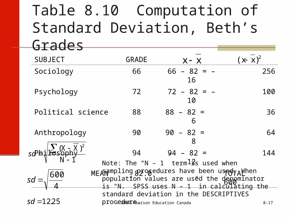
Table 8.10 Computation of Standard Deviation, Beth’s Grades
SUBJECT GRADE
Sociology 66 66 – 82 = –16 256
Psychology 72 72 – 82 = –10 100
Political science 88 88 – 82 = 6 36
Anthropology 90 90 – 82 = 8 64
Philosophy 94 94 – 82 = 12 144
MEAN 82.0 TOTAL 600
1 N
)XX( 2
sd
4
600sd
25.12sd
Note: The “N – 1” term is used when sampling procedures have been used. When population values are used the denominator is “N.” SPSS uses N – 1” in calculating the standard deviation in the DESCRIPTIVES procedure.
xx 2)x(x
8-18© 2007 Pearson Education Canada
Standardizing Data
Standardizing data facilitates making comparisons between units of different size Also, can standardize data to create variables
that have similar variability (Z scores) Standardization of data is commonly done
Several methods of standardizing data: proportions, percentages, percentage change, rates, ratios

8-19© 2007 Pearson Education Canada
Proportions
A proportion represents the part of 1 that some element represents.
Proportion female = Number female
Total persons
Proportion female = 31,216
58,520
Proportion female = .53
The females represent .53 of the population
8-20© 2007 Pearson Education Canada
Percentage
A percentage represents how often something happens per 100 times A proportion may be converted to a
percentage by multiplying by 100 Females constitute 53% of the population
8-21© 2007 Pearson Education Canada
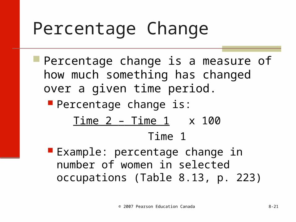
Percentage Change
Percentage change is a measure of how much something has changed over a given time period. Percentage change is:
Time 2 – Time 1 x 100
Time 1 Example: percentage change in number of
women in selected occupations (Table 8.13, p. 223)

8-22© 2007 Pearson Education Canada
Rates
Rates represent the frequency of an event for a standard-sized unit. Divorce rates, suicide rates, crime rates are examples. So if we had 104 suicides in a population of
757,465 the suicide rate per 100,000 would be calculated as follows:
SR = 104 x 100,000 = 13.73 757,465
There are 13.73 suicides per 100,000
8-23© 2007 Pearson Education Canada
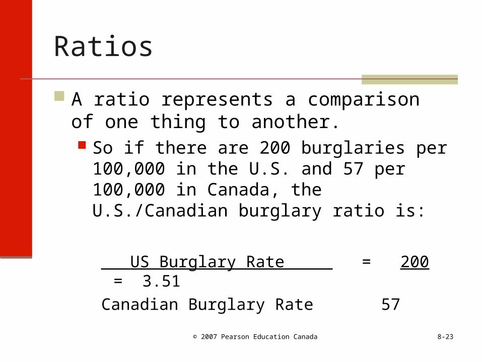
Ratios
A ratio represents a comparison of one thing to another. So if there are 200 burglaries per 100,000 in
the U.S. and 57 per 100,000 in Canada, the U.S./Canadian burglary ratio is:
US Burglary Rate = 200 = 3.51
Canadian Burglary Rate 57
8-24© 2007 Pearson Education Canada
Normal Distribution
Much data in the social and physical world are “normally distributed”; this means that there will be a few low values, many more clustered toward the middle, and a few high values.
Normal distributions: symmetrical, bell-shaped curve mean, mode, and median will be similar 68.28% of cases ± 1 standard deviation of mean 95.46% of cases ± 2 standard deviations of mean

8-25© 2007 Pearson Education Canada
Figure 8.2 Normal Distribution Curve

8-26© 2007 Pearson Education Canada
Z Scores
A Z score represents the distance from the mean, in standard deviation units, of any value in a distribution.
The Z score formula is as follows:
sd
XXZ
8-27© 2007 Pearson Education Canada
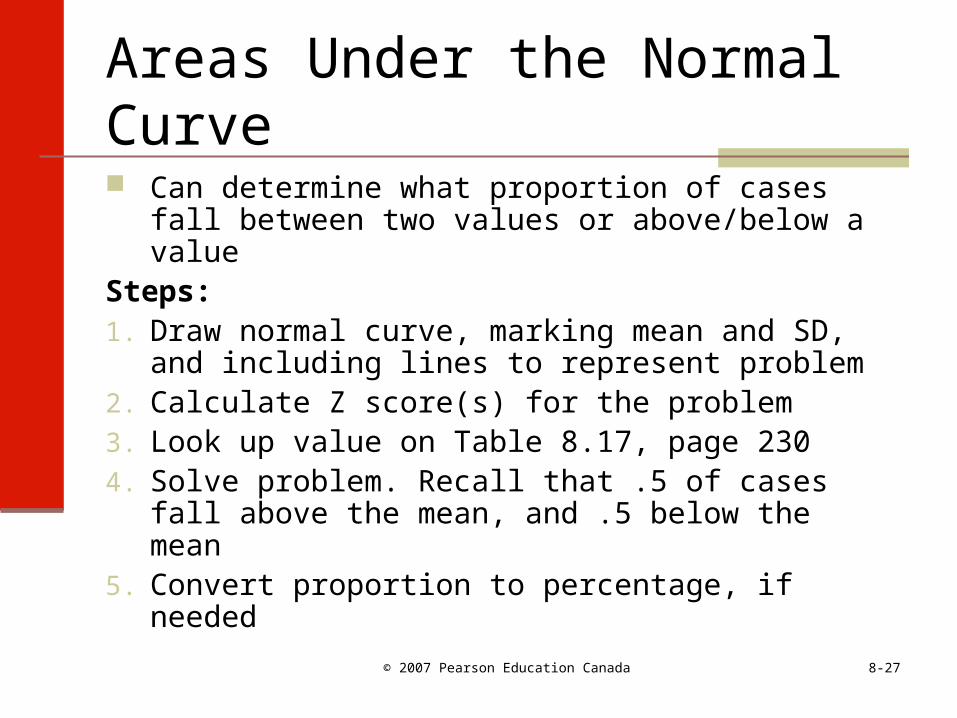
Areas Under the Normal Curve
Can determine what proportion of cases fall between two values or above/below a value
Steps:1. Draw normal curve, marking mean and SD,
and including lines to represent problem 2. Calculate Z score(s) for the problem3. Look up value on Table 8.17, page 2304. Solve problem. Recall that .5 of cases fall
above the mean, and .5 below the mean5. Convert proportion to percentage, if needed
8-28© 2007 Pearson Education Canada
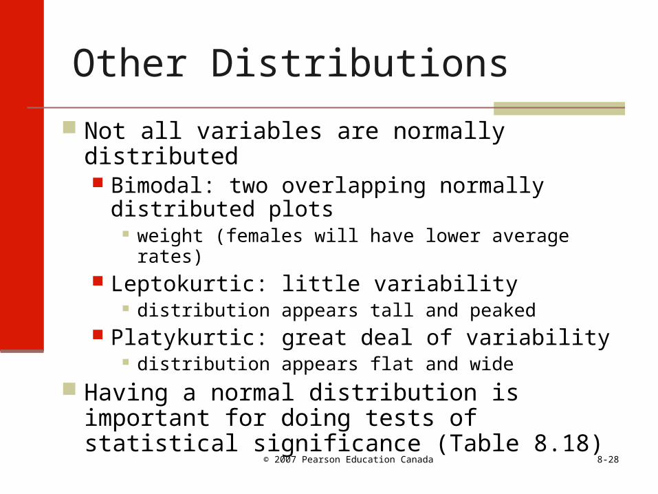
Other Distributions
Not all variables are normally distributed Bimodal: two overlapping normally distributed
plots weight (females will have lower average rates)
Leptokurtic: little variability distribution appears tall and peaked
Platykurtic: great deal of variability distribution appears flat and wide
Having a normal distribution is important for doing tests of statistical significance (Table 8.18)

8-29© 2007 Pearson Education Canada
Figure 8.4 Other Distributions
8-30© 2007 Pearson Education Canada
Describing Relationships Among Variables
Involves three important steps:
1. Decide which variable is to be treated as dependent variable and independent variable
2. Decide on the appropriate procedure for examining the relationship
3. Perform the analysis
8-31© 2007 Pearson Education Canada
Methods
Selection of statistical method depends upon the level of measurement of the dependent and independent variables
1. Contingency tables: Crosstabs
2. Comparing means: means analysis
3. Correlational analysis: correlation
8-32© 2007 Pearson Education Canada
Contingency Tables: Crosstabs
A contingency table cross-classifies cases on two or more variables to show the relation between an independent and dependent variable
Uses a nominal dependent variable and an ordinal or nominal independent variable
A standard table looks like the one on the following slide.
8-33© 2007 Pearson Education Canada
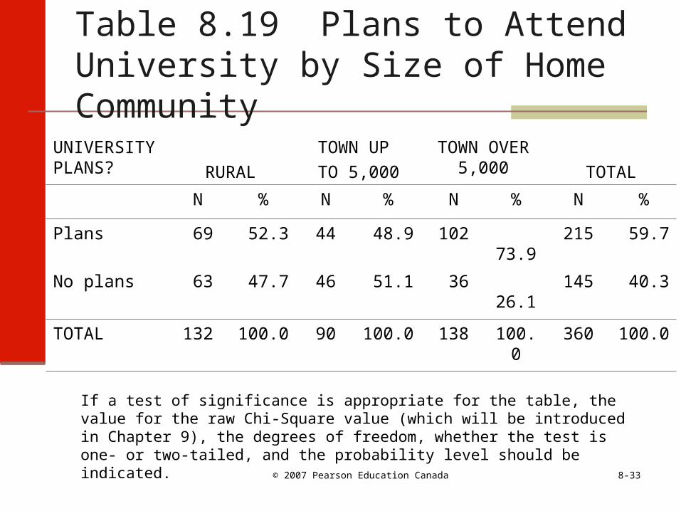
Table 8.19 Plans to Attend University by Size of Home Community
UNIVERSITY PLANS? RURAL
TOWN UP
TO 5,000
TOWN OVER 5,000 TOTAL
N % N % N % N %
Plans 69 52.3 44 48.9 102 73.9 215 59.7
No plans 63 47.7 46 51.1 36 26.1 145 40.3
TOTAL 132 100.0 90 100.0 138 100.0 360 100.0
If a test of significance is appropriate for the table, the value for the raw Chi-Square value (which will be introduced in Chapter 9), the degrees of freedom, whether the test is one- or two-tailed, and the probability level should be indicated.
8-34© 2007 Pearson Education Canada
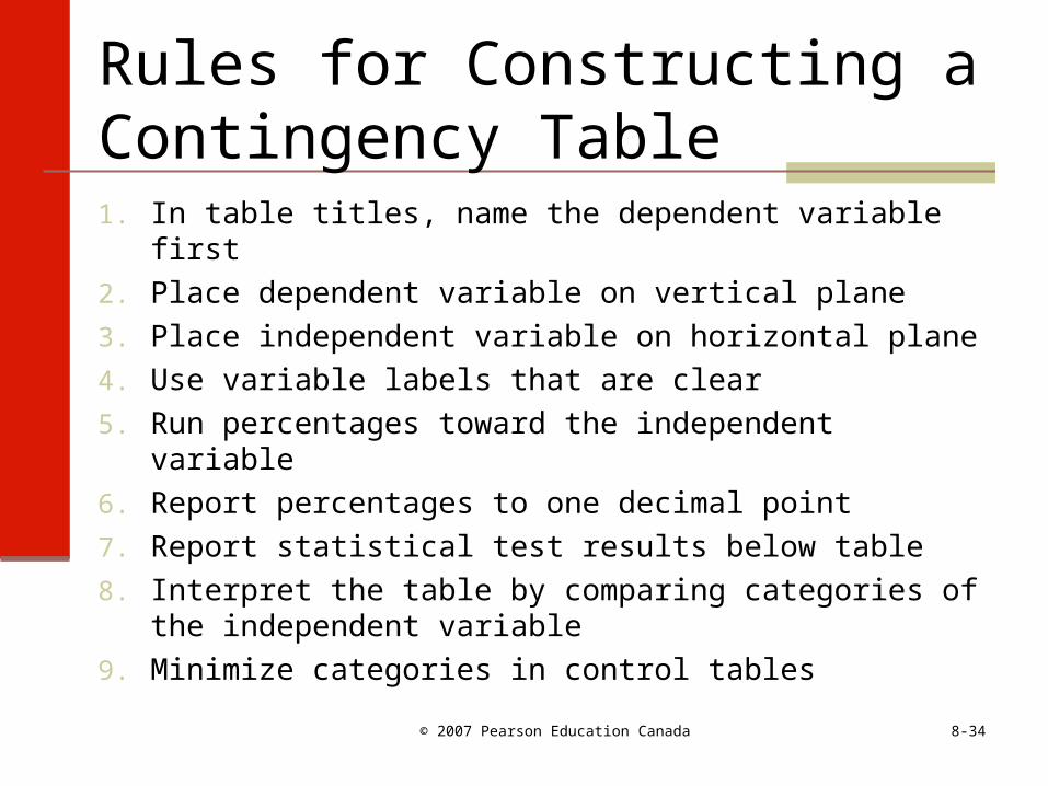
Rules for Constructing a Contingency Table1. In table titles, name the dependent variable first
2. Place dependent variable on vertical plane
3. Place independent variable on horizontal plane
4. Use variable labels that are clear
5. Run percentages toward the independent variable
6. Report percentages to one decimal point
7. Report statistical test results below table
8. Interpret the table by comparing categories of the independent variable
9. Minimize categories in control tables
8-35© 2007 Pearson Education Canada
Comparing Means: Means
Used when dependent variable is ratio Comparison to categories of independent
variable (nominal or ordinal) Both t-test and ANOVA may be used
(Chapter 9)
Presentation may be as shown on the following slide.
8-36© 2007 Pearson Education Canada
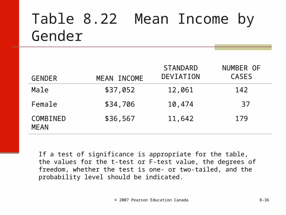
Table 8.22 Mean Income by Gender
GENDER MEAN INCOME
STANDARD DEVIATION
NUMBER OF CASES
Male $37,052 12,061 142
Female $34,706 10,474 37
COMBINED MEAN
$36,567 11,642 179
If a test of significance is appropriate for the table, the values for the t-test or F-test value, the degrees of freedom, whether the test is one- or two-tailed, and the probability level should be indicated.
8-37© 2007 Pearson Education Canada
Correlational Analysis: Correlation
Correlational analysis is a procedure for measuring how closely two ratio level variables co-vary together Basis for more advanced procedures: partial
correlations, multiple correlations, regression, factor analysis, path analysis and canonical analysis
Advantage: can analyze many variables (multivariate analysis) simultaneously Relies on having ratio level measures
8-38© 2007 Pearson Education Canada
Two Basic Concerns
1. What is the equation that describes the relation between two variables?
2. What is the strength of the relation between the two?
Two visual estimations procedures
A. The linear equation: Y = a + bX
B. Correlation coefficient: r
8-39© 2007 Pearson Education Canada
The Linear Equation
The linear equation, Y = a + bX, describes the relation between the two variables
Components:Y - dependent variable (e.g., starting salary)X - independent variable (e.g., years of post-
secondary education)a - the constant, which indicates where the
regression line intersects the Y-axisb - the slope of the regression line

8-40© 2007 Pearson Education Canada
A. The Linear Equation:A Visual Estimation ProcedureStep 1: Plot the relation on
a graph
Table 8.24: Sample data set
X Y 2 3
3 45 47 68 8
8-41© 2007 Pearson Education Canada
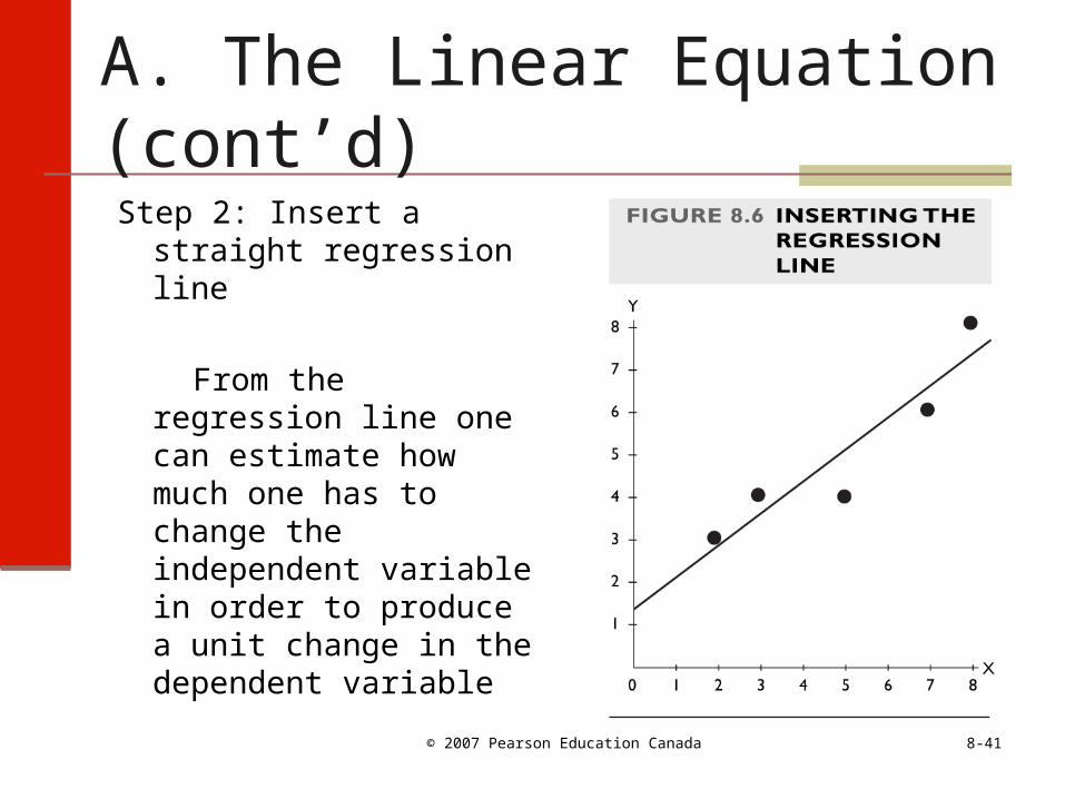
A. The Linear Equation (cont’d)
Step 2: Insert a straight regression line
From the regression line one can estimate how much one has to change the independent variable in order to produce a unit change in the dependent variable
8-42© 2007 Pearson Education Canada
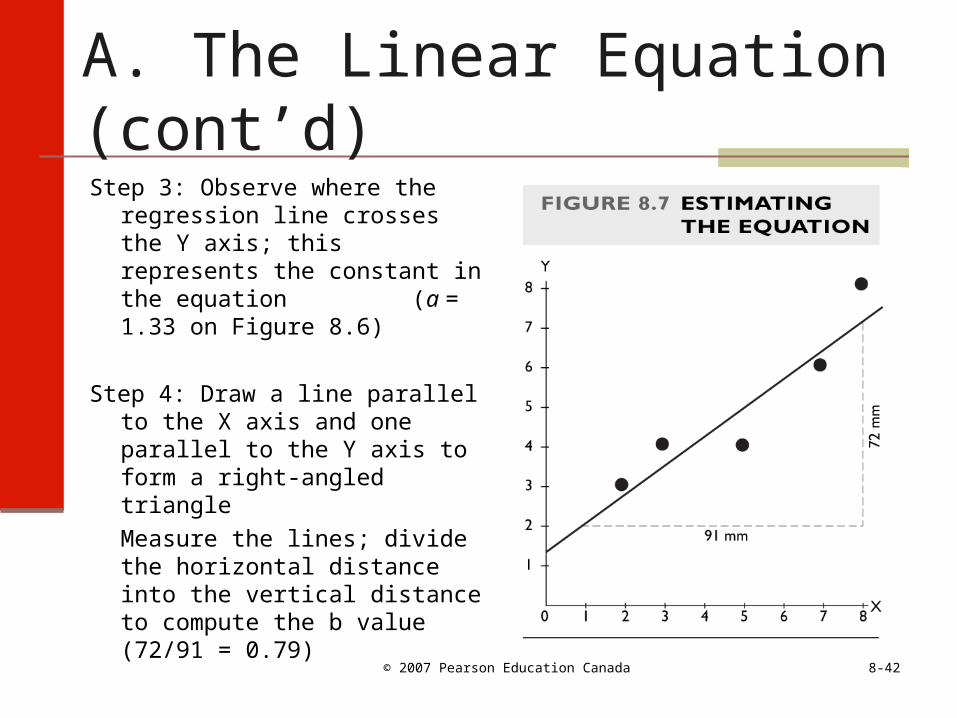
A. The Linear Equation (cont’d)
Step 3: Observe where the regression line crosses the Y axis; this represents the constant in the equation (a = 1.33 on Figure 8.6)
Step 4: Draw a line parallel to the X axis and one parallel to the Y axis to form a right-angled triangle
Measure the lines; divide the horizontal distance into the vertical distance to compute the b value (72/91 = 0.79)
8-43© 2007 Pearson Education Canada
A. The Linear Equation (cont’d)
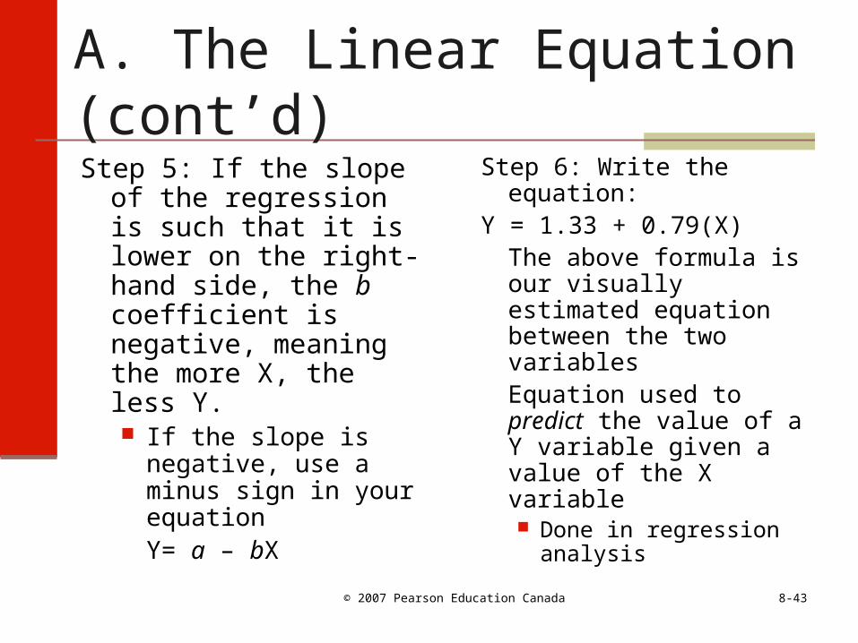
Step 5: If the slope of the regression is such that it is lower on the right-hand side, the b coefficient is negative, meaning the more X, the less Y. If the slope is negative,
use a minus sign in your equationY= a – bX
Step 6: Write the equation:Y = 1.33 + 0.79(X)
The above formula is our visually estimated equation between the two variablesEquation used to predict the value of a Y variable given a value of the X variable Done in regression
analysis
8-44© 2007 Pearson Education Canada
B. Correlation Coefficient: A Visual Estimation Procedure Goal: to develop a sense of what correlations
of different magnitudes look like Correlation coefficient (r) is a measure of the
strength of the association between two variables Vary from +1 to –1 Perfect correlations are rare Usually presented by a decimal point, as
in .98, .56, –.32 Negative correlations ~ negative slope

8-45© 2007 Pearson Education Canada
Figure 8.9 Eight Linear Correlations
8-46© 2007 Pearson Education Canada
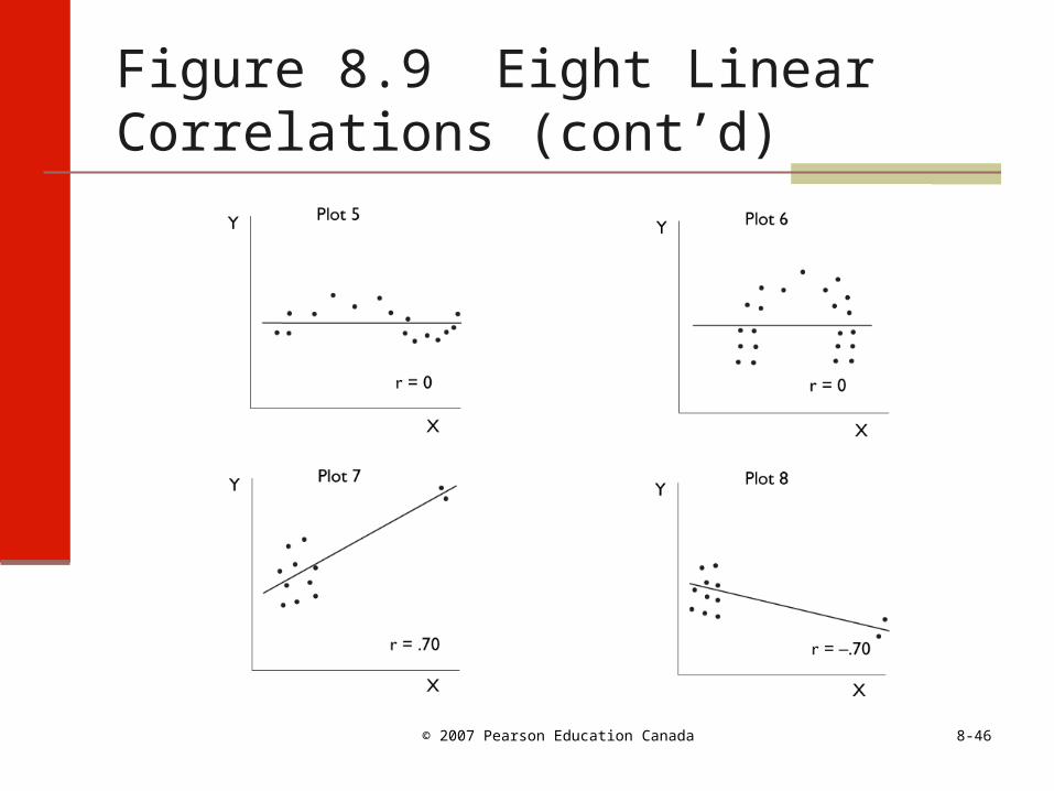
Figure 8.9 Eight Linear Correlations (cont’d)
8-47© 2007 Pearson Education Canada
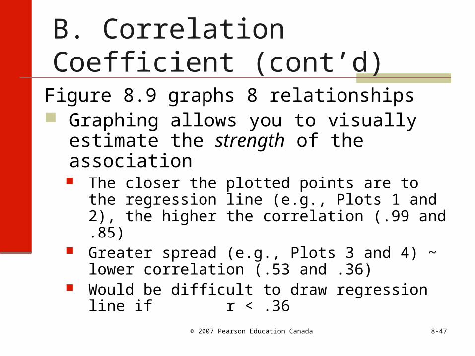
B. Correlation Coefficient (cont’d)
Figure 8.9 graphs 8 relationships Graphing allows you to visually estimate
the strength of the association The closer the plotted points are to the
regression line (e.g., Plots 1 and 2), the higher the correlation (.99 and .85)
Greater spread (e.g., Plots 3 and 4) ~ lower correlation (.53 and .36)
Would be difficult to draw regression line if r < .36
8-48© 2007 Pearson Education Canada
B. Correlation Coefficient (cont’d)
Plots 5 and 6: curvilinear: not linear, hence r = 0
Procedure not appropriate for curvilinear relations Plots 7 and 8: problem plots: deviant cases
This is one of the reasons it is important to plot relationships; extreme values indicate a non-linear relationship, therefore linear regression procedure are not appropriate for studying these relationships

8-49© 2007 Pearson Education Canada
Calculating the Correlation Coefficient The estimation of the correlation coefficient
takes two kinds of variability into account:1. Variations around the regression line2. Variations around the mean of Y
r2 = 1 – variations around regression variations around mean of Y
Can calculate (see p. 245); computer programs used by most researchers today

8-50© 2007 Pearson Education Canada
Other Correlation Procedures
Spearman Correlation Appropriate measure of association for ordinal
level variables Partial Correlation
Measures the strength of association between two variables while simultaneously controlling for the effects of one or more additional variables
Also varies from +1 to –1 Commonly used by social researchers