CHARACTERISTICS OF A SERIES OF HIGH SPEED HARD CHINE PLANING

HULLS - PART II: PERFORMANCE IN WAVES.

D.J. Taunton, Fluid-Structure Interaction Research Group, School of Engineering Sciences, University of Southampton

D.A. Hudson, Fluid-Structure Interaction Research Group, School of Engineering Sciences, University of Southampton

R.A. Shenoi, Fluid-Structure Interaction Research Group, School of Engineering Sciences, University of Southampton

SUMMARY

An experimental investigation into the performance of high speed hard chine planing hulls in irregular waves has been

conducted. A new series of models representative of current design practice was developed and tested experimentally.

Measurements of the rigid body motions and accelerations were made at three speeds in order to assess the influence of

fundamental design parameters on the seakeeping performance of the hulls and human factors performance of the crew,

with an aim to provide designers with useful data.

Response data, such as heave and pitch motions and accelerations, are presented as probability distributions due to the

non-linear nature of high speed craft motions. Additionally statistical parameters for the experimental configurations

tested are provided and the most relevant measures for crew performance discussed. Furthermore, an example of the use

of these statistical parameters to evaluate the vibration dose value of the crew onboard a full scale high speed planing

craft is given. It is confirmed that at high speed craft motion leads to recommended maximum values of vibration dose

value being exceeded after only short durations. In practice, therefore, mitigating strategies need to be developed and/or

employed to reduce crew exposure to excessive whole body vibration.

NOMENCLATURE

Deadrise [o]

Displaced volume [m3]

Displaced veight [N]

Wave amplitude [m]

Pitch [°]

λ Ship scale factor

Ship heading relative to waves []

e Wave encounter frequency [rad/s]

0 Wave frequency [rad/s]

az Vertical acceleration [m/s2]

B Beam [m]

CV Speed coefficient CV=V/(g.B)0.5

g Acceleration due to gravity 9.80665m/s2

Gyy Pitch radius of gyration [%L]

H1/3 Significant wave height [m]

L Length over all [m]

LCG Longitudinal centre of gravity [%L] from

transom

L/1/3 Length-displacement ratio

t Time [s]

T Draught [m]

Tz Zero crossing period [s]

V Speed [m/s]

Z Heave at LCG [m]

1 INTRODUCTION

The operation of small, high speed craft for military,

commercial and leisure use has increased dramatically in

recent years. These craft are usually of hard chine form

and designed to plane. The development of light weight

propulsion systems and engines has resulted in an

increase in the typical operational speed of such craft.

Extensive research into material properties and

construction techniques has led to stronger hulls, with the

consequence that the limiting factor in practical

operations is now more likely to be the people operating

the vessel. Anecdotal and survey evidence from operators

of high speed craft, for example that carried out by the

US Navy into their special forces [1], has shown a high

probability of serious injury.

The legislative framework for ‘whole body vibration’ in

the European Union [2] prescribes minimum standards

for the health and safety of workers exposed to vibration.

Although the research under-pinning the directive was

principally carried out for the land transport industry, the

standards apply to all workplaces including high speed

craft. When applied to accelerations typically

experienced on high speed craft it is seen that

recommended maximum vibration levels are exceeded in

a very short time, as shown in this work. This implies a

need to assess such acceleration levels for typical

operations and take mitigating action where necessary.

For existing craft such action may include modification

to operating procedures, crew training and fitting of

alternative seat configurations or ride control systems.

For new craft the opportunity exists to consider the

effects of various craft design parameters on the levels of

accelerations the crew will be exposed to. However,

there is little such data in the public domain. This study

presents experimentally derived data for a series of high

speed hard chine planing hulls in waves, in a form that

may be used by designers of such craft. The experiments

are described and the analysis procedure adopted

detailed. Results for a range of design parameters,

including length-displacement ratio and radius of

gyration, together with design features, such as transverse

steps, are presented. An example of the use of these data

for assessing acceleration levels for a full scale craft is

also included.

2 DESCRIPTION OF MODELS

The availability of experimental data for the seakeeping

performance of high speed planing hulls is limited. The

most significant investigations into performance of

planing craft in waves are those by Fridsma [3, 4] on a

series of prismatic hull forms. This investigation covered

the influence of length-to-beam ratio, deadrise angle,

operating speed and wave height together with trim and

load. These tests were later extended by Zarnick [5] to

cover a greater range of length-beam ratios.

Other seakeeping experiments of high speed planing craft

include those conducted by Rosen and Garme [6, 7] on a

specific hull design. The seakeeping performance of a

double-chined planing hull suitable for high speed ferry

applications has been investigated by Grigoropoulos [8],

but the speed range is too low for small high speed craft.

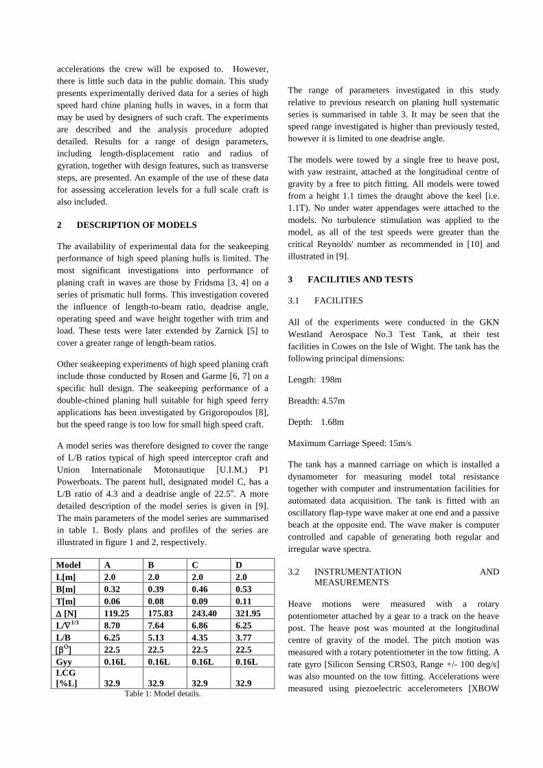
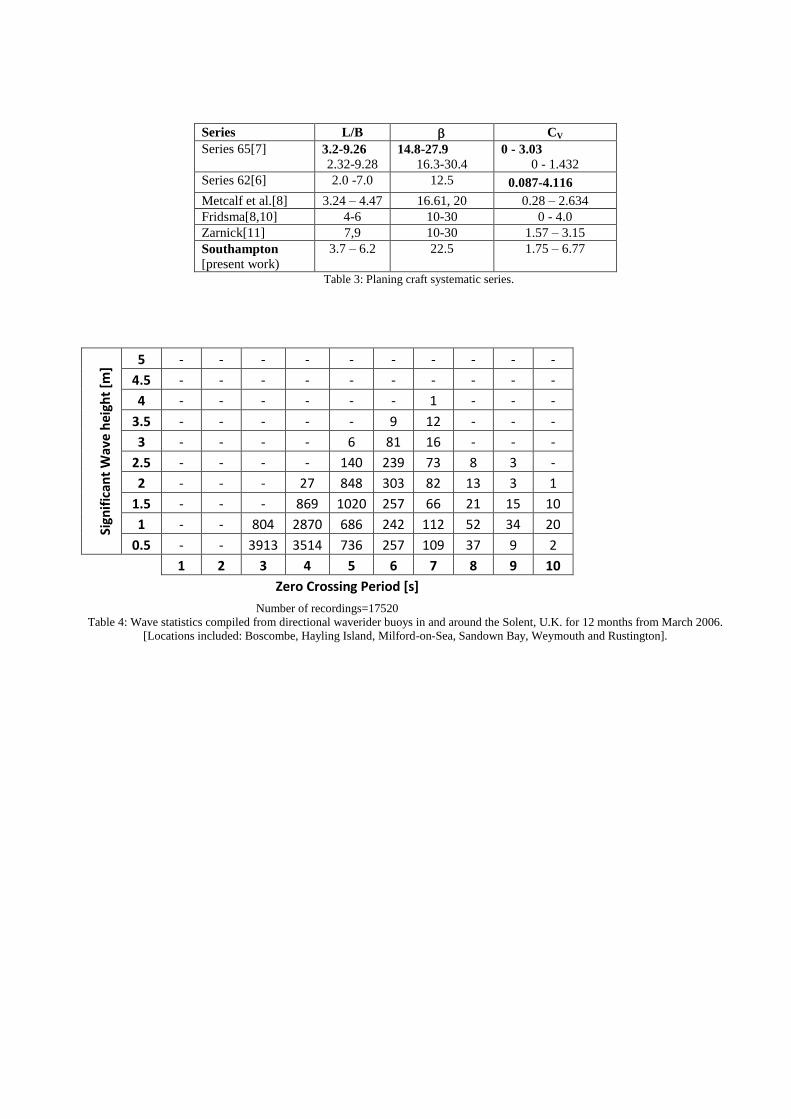
A model series was therefore designed to cover the range

of L/B ratios typical of high speed interceptor craft and

Union Internationale Motonautique [U.I.M.) P1

Powerboats. The parent hull, designated model C, has a

L/B ratio of 4.3 and a deadrise angle of 22.5o. A more

detailed description of the model series is given in [9].

The main parameters of the model series are summarised

in table 1. Body plans and profiles of the series are

illustrated in figure 1 and 2, respectively.

Model A B C D

L[m] 2.0 2.0 2.0 2.0

B[m] 0.32 0.39 0.46 0.53

T[m] 0.06 0.08 0.09 0.11

[N] 119.25 175.83 243.40 321.95

L/1/3 8.70 7.64 6.86 6.25

L/B 6.25 5.13 4.35 3.77

22.5 22.5 22.5 22.5

Gyy 0.16L 0.16L 0.16L 0.16L

LCG

[%L] 32.9 32.9 32.9 32.9 Table 1: Model details.

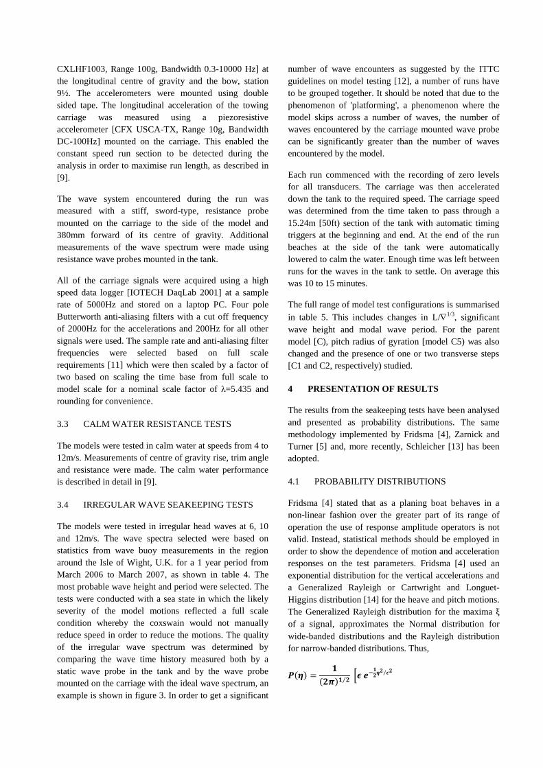
The range of parameters investigated in this study

relative to previous research on planing hull systematic

series is summarised in table 3. It may be seen that the

speed range investigated is higher than previously tested,

however it is limited to one deadrise angle.

The models were towed by a single free to heave post,

with yaw restraint, attached at the longitudinal centre of

gravity by a free to pitch fitting. All models were towed

from a height 1.1 times the draught above the keel [i.e.

1.1T). No under water appendages were attached to the

models. No turbulence stimulation was applied to the

model, as all of the test speeds were greater than the

critical Reynolds' number as recommended in [10] and

illustrated in [9].

3 FACILITIES AND TESTS

3.1 FACILITIES

All of the experiments were conducted in the GKN

Westland Aerospace No.3 Test Tank, at their test

facilities in Cowes on the Isle of Wight. The tank has the

following principal dimensions:

Length: 198m

Breadth: 4.57m

Depth: 1.68m

Maximum Carriage Speed: 15m/s

The tank has a manned carriage on which is installed a

dynamometer for measuring model total resistance

together with computer and instrumentation facilities for

automated data acquisition. The tank is fitted with an

oscillatory flap-type wave maker at one end and a passive

beach at the opposite end. The wave maker is computer

controlled and capable of generating both regular and

irregular wave spectra.

3.2 INSTRUMENTATION AND

MEASUREMENTS

Heave motions were measured with a rotary

potentiometer attached by a gear to a track on the heave

post. The heave post was mounted at the longitudinal

centre of gravity of the model. The pitch motion was

measured with a rotary potentiometer in the tow fitting. A

rate gyro [Silicon Sensing CRS03, Range +/- 100 deg/s]

was also mounted on the tow fitting. Accelerations were

measured using piezoelectric accelerometers [XBOW

CXLHF1003, Range 100g, Bandwidth 0.3-10000 Hz] at

the longitudinal centre of gravity and the bow, station

9½. The accelerometers were mounted using double

sided tape. The longitudinal acceleration of the towing

carriage was measured using a piezoresistive

accelerometer [CFX USCA-TX, Range 10g, Bandwidth

DC-100Hz] mounted on the carriage. This enabled the

constant speed run section to be detected during the

analysis in order to maximise run length, as described in

[9].

The wave system encountered during the run was

measured with a stiff, sword-type, resistance probe

mounted on the carriage to the side of the model and

380mm forward of its centre of gravity. Additional

measurements of the wave spectrum were made using

resistance wave probes mounted in the tank.

All of the carriage signals were acquired using a high

speed data logger [IOTECH DaqLab 2001] at a sample

rate of 5000Hz and stored on a laptop PC. Four pole

Butterworth anti-aliasing filters with a cut off frequency

of 2000Hz for the accelerations and 200Hz for all other

signals were used. The sample rate and anti-aliasing filter

frequencies were selected based on full scale

requirements [11] which were then scaled by a factor of

two based on scaling the time base from full scale to

model scale for a nominal scale factor of λ=5.435 and

rounding for convenience.

3.3 CALM WATER RESISTANCE TESTS

The models were tested in calm water at speeds from 4 to

12m/s. Measurements of centre of gravity rise, trim angle

and resistance were made. The calm water performance

is described in detail in [9].

3.4 IRREGULAR WAVE SEAKEEPING TESTS

The models were tested in irregular head waves at 6, 10

and 12m/s. The wave spectra selected were based on

statistics from wave buoy measurements in the region

around the Isle of Wight, U.K. for a 1 year period from

March 2006 to March 2007, as shown in table 4. The

most probable wave height and period were selected. The

tests were conducted with a sea state in which the likely

severity of the model motions reflected a full scale

condition whereby the coxswain would not manually

reduce speed in order to reduce the motions. The quality

of the irregular wave spectrum was determined by

comparing the wave time history measured both by a

static wave probe in the tank and by the wave probe

mounted on the carriage with the ideal wave spectrum, an

example is shown in figure 3. In order to get a significant

number of wave encounters as suggested by the ITTC

guidelines on model testing [12], a number of runs have

to be grouped together. It should be noted that due to the

phenomenon of 'platforming', a phenomenon where the

model skips across a number of waves, the number of

waves encountered by the carriage mounted wave probe

can be significantly greater than the number of waves

encountered by the model.

Each run commenced with the recording of zero levels

for all transducers. The carriage was then accelerated

down the tank to the required speed. The carriage speed

was determined from the time taken to pass through a

15.24m [50ft) section of the tank with automatic timing

triggers at the beginning and end. At the end of the run

beaches at the side of the tank were automatically

lowered to calm the water. Enough time was left between

runs for the waves in the tank to settle. On average this

was 10 to 15 minutes.

The full range of model test configurations is summarised

in table 5. This includes changes in L/1/3

, significant

wave height and modal wave period. For the parent

model [C), pitch radius of gyration [model C5) was also

changed and the presence of one or two transverse steps

[C1 and C2, respectively) studied.

4 PRESENTATION OF RESULTS

The results from the seakeeping tests have been analysed

and presented as probability distributions. The same

methodology implemented by Fridsma [4], Zarnick and

Turner [5] and, more recently, Schleicher [13] has been

adopted.

4.1 PROBABILITY DISTRIBUTIONS

Fridsma [4] stated that as a planing boat behaves in a

non-linear fashion over the greater part of its range of

operation the use of response amplitude operators is not

valid. Instead, statistical methods should be employed in

order to show the dependence of motion and acceleration

responses on the test parameters. Fridsma [4] used an

exponential distribution for the vertical accelerations and

a Generalized Rayleigh or Cartwright and Longuet-

Higgins distribution [14] for the heave and pitch motions.

The Generalized Rayleigh distribution for the maxima ξ

of a signal, approximates the Normal distribution for

wide-banded distributions and the Rayleigh distribution

for narrow-banded distributions. Thus,

( )

( ) ⁄ [

⁄

( )

∫ ( )

⁄

] (1)

where

and

as ε0 resulting in a Rayleigh Distribution,

( ) (2)

whereas for ε1 resulting in a Normal Distribution,

( )

)

(3)

In the analysis of the experimental results in this study, it

was found that a Gamma distribution fitted the

acceleration data better than an exponential distribution.

The exponential distribution is a particular case of the

Gamma distribution, [when α=1). That is,

Gamma Distribution

( ) {

⁄

)

(4)

where ( ) ∫

Exponential Distribution

( ) {

⁄

(5)

The analysis process adopted is as follows:

1) The test runs which comprise a single test

condition are loaded and the mean of each run is

removed before the runs joined to produce a

single time trace for a given test condition.

2) A peak detection algorithm, as used by Allen et

al. [11], is used to find the peaks in the time

trace. These peaks are grouped into either

maxima or minima. For the case of accelerations

the minima are used because they represent the

deceleration on impact with the water.

3) The maxima or minima are sorted into

ascending order.

4) The proportion, r, of negative maxima to total

maxima is determined, or in the case of minima

the proportion of positive minima to total

minima determined.

5) The r value is used to determine the spectral

width of the spectrum, ε.

) (6)

6) The sorted maxima or minima are grouped into

15 equal width bins and a histogram plotted.

7) For the wave height distributions and vessel

motion a Cartwright and Longuet-Higgins

probability density function [14] is used to

determine the expected values for the particular

condition. For the vertical acceleration

distributions a Gamma probability density

function is used to determine the expected

values.

8) A χ2 goodness of fit calculation is determined.

4.2 STATISTICS

The use of statistics as a means to compare different

hullforms in the same sea state is useful, as it provides a

single number with which to compare the hulls. A

number of the statistics commonly used are required for

assessing the performance of high speed planing craft

under the EU directive on whole body vibration [2].

However, it should be noted that under the EU directive

acceleration values need to be weighted and this is only

possible for data acquired at full scale. Statistical

measures relevant to high speed craft motions may thus

be summarised as,

Root mean square

[

∑ ( )]

⁄

(7)

Root mean quad

[

∑ ( )]

⁄

(8)

Vibration dose value

[

∑ ( )]

⁄

(9)

Crest Factor

Is the peak value divided by the rms.

4.3 VIBRATION DOSE VALUE AND HUMAN

FACTORS.

Traditionally naval architects have used statistics such as

motion sickness incidence [MSI), subjective magnitude

[SM) and motion induced interruptions [MII) as

measures of human performance [15]. These measures

are either not applicable to small high speed craft, where

the crew are usually seated, or have been superseded by

more recent and relevant measures.

For example, the measure of motion sickness now uses

the motion sickness dose value described in ISO 2631-1

[16]. Motion induced interruptions are not usually

applicable to seated crew and the subjective magnitude

measure could now be replaced by the vibration dose

value [VDV) as described in ISO 2631-1 or the spinal

response acceleration dose described in ISO-2631-5 [17].

Whilst these new measures were not developed

specifically for assessing the human performance on

board ships, they have been developed to quantify human

performance in a variety of transport methods and this

facilitates ready comparison between them and between

human performance in different occupations. There has

been debate recently as to the applicability of these

measures to the assessment of small boat performance

[18, 19], especially since VDV has been implemented as

one of the measures in an EU directive on whole body

vibration [2]. The reasoning behind the debate on the

applicability of VDV is that there is a high prevalence of

injury among high speed craft crew [1] and vibration

dose value was developed for quantifying performance

degradation rather than injury. The magnitude of the

accelerations used to validate the vibration dose value

model for use in human factors were also much smaller

than those typically encountered in high speed craft

operation.

A means of comparing the performance of different

hullforms is still required, however, and until a more

suitable method of evaluating high speed craft is

developed and validated, VDV is probably the most

suitable measure of performance. A number of

investigations have been conducted into the vibration

dose values of different vehicles, including powerboats

and RIBs [20, 21]. A pilot study into the human

performance degradation due to simulated slamming

conducted by Wolk [22] concluded that human

performance reduced with increasing slam magnitude and

frequency.

5 DISCUSSION OF RESULTS

Example motion and acceleration time traces are

presented in figures 4 to 7 for model C in configuration

12 of table 5. That is, at a model speed of 6.25m/s in a

JONSWAP spectrum corresponding to a full scale H1/3 of

0.5m and modal period of 6s, based on a nominal scale

factor of λ=5.435. The full scale speed for this condition

is thus 14.57 m/s, or 28.32 knots. It can be seen from

figure 4 that the heave motion is similar in frequency to

the wave amplitude, which is supported by the power

spectral density plot in figure 8. In comparison, the

vertical acceleration time traces shown in figures 6 and 7

illustrate that the trace consists of repeated shock

impacts. The example acceleration power spectral density

in figure 9 shows a second peak at an encounter

frequency of 1.5Hz.

Figures 10 to 16 show examples of the histograms and

fitted probability distribution functions for wave height,

heave maxima, heave minima, pitch maxima, pitch

minima and centre of gravity and bow acceleration

minima for the parent model [C) at one speed and

travelling in one irregular sea state. For all the model

configurations tested [table 5), all parameters for the

relevant probability distributions are presented in table 6.

These data allow the probability distribution for any

model configuration in table 5 to be re-created in a

manner similar to the examples presented in figure 10 to

16. Once the probability distribution for the motion

responses is known, the probability of any motion

variable exceeding a particular value may readily be

found. These data are thus of direct use for designers of

such high speed craft.

A linear regression model has been fitted to the

experimental data to show the relationship between

length-displacement ratio, speed coefficient Cv and RMS

vertical accelerations at the longitudinal centre of gravity

[LCG) and the bow. The results are plotted in figure 17

and 18 and the regression equations are given as,

(

)

(

)

(

)

(

)

(

) (

)

(10)

RMS Acceleration

at LCG

RMS Acceleration at

Bow

C 154.5 291.6

C1 2.6 4.9

C2 9.8 17.8

C3 0.2 0.3

C4 -1.5 -2.8

C5 -2.6 -4.9

C6 -41.2 -77.2

C7 -85.3 -155.6

C8 23.0 43.0

Table 2: Regression coefficients for RMS vertical acceleration

in equation 10.

The influence of transverse steps on the RMS vertical

accelerations for model C at three speeds is presented in

figure 19. This figure indicates that steps have virtually

no influence on the RMS accelerations.

The influence of wave height on the RMS accelerations

for model C are presented in figure 20. This shows a non

linear relationship for the LCG accelerations, with little

change in acceleration for increasing wave height and an

almost linear relationship for the bow accelerations.

6 DESIGN APPLICATIONS

In order to allow the model data to be used to predict the

human performance onboard a full scale vessel, tables of

RMS and RMQ accelerations are presented in table 7.

The RMS and RMQ values have been weighted using the

weighting Wb as described in ISO 2631-1 [16]. This

process involved scaling the model test data to a nominal

full scale, applying the weighting and then scaling the

weighted data back to model scale. The weighted RMS

and RMQ accelerations were next calculated at the

longitudinal centre of gravity and bow. Using the RMQ it

is possible to calculate the VDV as,

⁄ (11)

The duration, t, is a function of scale factor, R0.5

, which

means that it is possible to calculate the VDV for any

other scale of vessel by multiplying the RMQ by

[t·R0.5

)1/4

.

The estimated time to exceed a given VDV limit, such as

the daily exposure action value [9.1 m/s1.75

) and the daily

exposure limit [21 m/s1.75

) given in the EU Directive on

whole body vibration [2] can be calculated using

equation 12,

(12)

An example to illustrate how the model data may be used

to determine full-scale seakeeping performance and

assessment against the EU directive on whole body

vibration [2] is given below:

The example given is for a full scale vessel similar to

model C2 with a length of 15m. This results in a scale

factor of λ=7.5. The vessel has a design speed of 65

knots.

1) Select the most appropriate model configuration

from table 5, in this case configuration 32.

2) Use the corresponding values of weighted RMS

and RMQ vertical accelerations from table 7. In

this example RMS at LCG is 8.09 ms-2

and the

RMQ at LCG is 10.84 ms-2

. The duration of the

model runs was 11.68 s.

3) The model run duration is scaled from model to

full scale. Tfull=Tmodel×λ0.5

, in this case,

Tfull=11.68 × 2.74

Tfull=31.99 s

4) The full scale vibration dose value [VDV) can

then be calculated using equation 11 as

VDVfull = 10.84 × 31.991/4

VDVfull=25.78 ms-1.75

5) The time to exceed the 8 hour daily exposure

limit, given in the EU directive [2], of 21 ms-1.75

is then calculated from equation 12:

Time to the VDV limit of 21 m s-1.75

= 14.09s

7 CONCLUSIONS

An extensive experimental investigation into the motions

of small high speed craft in waves has been completed

through model scale testing. A new series of hard chine

planing hulls representative of modern practice was

designed to allow the influence of L/1/3

on the

behaviour of such craft in waves to be studied. The

models were tested at three speeds. In addition a limited

investigation into the effects of transverse steps, radius of

gyration, wave height and wave period on the craft

motions in waves was undertaken.

Due to the non-linearity of planing craft motions in

waves probability distributions are fitted to heave and

pitch motions and accelerations at the centre of gravity

and bow. These distributions allow comparisons between

model configurations and prediction of occurrence of

extremes to be made. Such data are presented in a form

useful to designers selecting appropriate hull forms.

Statistical data for each configuration tested also enables

predictions of measures of human performance for crew

onboard such small high speed craft. An example of the

use of these data for predicting vibration dose value for

crew at full scale is given. This confirms that exposure to

these levels of vibration onboard small, fast craft leads to

crew exceeding rapidly the limits prescribed in EU

legislation.

For designers of high speed craft this implies that

mitigation of the levels of vibration should be sought.

Such mitigation may comprise, but is not limited to, hull

design, active ride control systems, seat design, training

methods and operating procedures.

8 REFERENCES

[1] W. ENSIGN, J. A. HODGDON, W. K.

PRUSACZYK, D. SHAPIRO, and M. LIPTON,

'A Survey of Self-Reported injuries Among

Special Boat Operators', Naval Health Research

Center, Report No. 00-48, 2000.

[2] 'DIRECTIVE 2002/44/EC OF THE

EUROPEAN PARLIAMENT AND OF THE

COUNCIL of 25 June 2002 on the minimum

health and safety requirements regarding the

exposure of workers to the risks arising from

physical agents [vibration) [sixteenth individual

Directive within the meaning of Article 16[1) of

Directive 89/391/EEC)'. Council of European

Union, Ed., 2002.

[3] G. FRIDSMA, 'A systematic study of the rough-

water performance of planing boats', Stevens

Institute of Technology, Report No. 1275, 1969.

[4] G. FRIDSMA, 'A systematic study of the rough-

water performance of planing boats [Irregular

Waves - Part II)', Stevens Institute of

Technology, Report No. 1495, 1971.

[5] E. E. ZARNICK and C. R. TURNER, 'Rough

water performance of high length to beam ratio

planing boats', David W. Taylor Naval Ship

Research and Development Center, Bethesda,

Maryland, Report No. DTNSRDC/SPD-0973-

01, 1981.

[6] A. ROSEN, 'Loads and responses for planing

craft in waves', in Division of naval Systems,

Aeronautical and Vehicle Engineering. PhD

Stockholm: KTH, 2004.

[7] A. ROSEN and K. GARME, 'Model experiment

addressing the impact pressure distribution on

planing craft in waves', Transactions of the

Royal Institution of Naval Architects, Volume

146, 2004.

[8] G. J. GRIGOROPOULOS, S. HARRIES, D. P.

DAMALA, L. BIRK, and J. HEIMANN,

'Seakeeping assessment for high-speed

monohulls - A comparative study.', Int. Marine

Design Conf. IMDC, Volume 1, pp. 137-148,

2003.

[9] D. J. TAUNTON, D. A. HUDSON, and R. A.

SHENOI, 'Characteristics of a series of high

speed hard chine planing hulls - Part I:

Performance in calm water.', International

Journal of Small Craft Technology, Volume 152,

Part B2, pp55-75, 2010.

[10] 'Testing and Extrapolation Methods, High Speed

Marine Vehicles, Resistance Test', in ITTC -

Recommended Procedures and Guidelines,

2002, p. 18.

[11] D. P. ALLEN, D. J. TAUNTON, and R.

ALLEN, 'A study of shock impacts and

vibration dose values onboard highspeed marine

craft', International Journal of Maritime

Engineering, Volume 150, pp. 10, 2008.

[12] 'Testing and Extrapolation Methods, High Speed

Marine Vehicles, Sea Keeping Tests', in ITTC -

Recommended Procedures and Guidelines. vol.

7.5-02-05-04, 2002, p. 13.

[13] D. M. SCHLEICHER, 'Regarding statistical

relationships for vertical accelerations of

planing monohulls in head seas', in High speed

craft - ACV's, WIG's & Hydrofoils. London:

RINA, 2006.

[14] D. E. CARTWRIGHT and M. S. LONGUET-

HIGGINS, 'The statistical distribution of the

maxima of a random function', Proceedings of

the Royal Society of London. Series A,

Mathematical and Physical Sciences, Volume

237, pp. 21, 1956.

[15] A. LLOYD, 'Seakeeping: Ship Behaviour in

Rough Weather', Revised ed.: ARJM Lloyd,

ISBN 0953263401, 1998.

[16] INTERNATIONAL ORGANISATION FOR

STANDARDISATION, 'Mechanical vibration

and shock - Evaluation of human exposure to

whole-body vibration -Part 1: General

requirements.', ISO 2631-1:1997[E).

[17] INTERNATIONAL ORGANISATION FOR

STANDARDISATION, 'Mechanical vibration

and shock —Evaluation of human exposure to

wholebody vibration — Part 5: Method for

evaluation of vibration containing multiple

shocks.', ISO 2631-5:2003[E).

[18] R. CRIPPS, S. REES, H. PHILLIPS, C. CAIN,

D. RICHARDS, and J. CROSS, 'Development

of a crew seat system for high speed craft', in

Seventh International Conference on Fast Sea

Transportation, FAST 2003. Ischia, Italy, 2003.

[19] R. GOLLWITZER and R. PETERSON,

'Repeated Water Entry Shocks on High-Speed

Planing Boats', Dahlgren Division, Naval

Surface Warfare Center, Panama City, Report

No. CSS/TR-96/27, 1995.

[20] C. H. LEWIS and M. J. GRIFFIN, 'A

comparison of evaluations and assessments

obtained using alternative standards for

predicting the hazards of whole-body vibration

and repeated shocks.', Journal of Sound and

Vibration, Volume 215, pp. 915-926, 1998.

[21] G. S. PADDAN and M. J. GRIFFIN, 'Evaluation

of whole-body vibration in vehicles', Journal of

Sound and Vibration, Volume 253, pp. 195-213,

2002.

[22] H. WOLK and J. F. TAUBER, 'Man's

Performance Degradation during Simulated

Small Boat Slamming ', Naval Ship Research

and Development Center, Bethesda, Report No.

4234, 1974.

Series L/B CV

Series 65[7] 3.2-9.26

2.32-9.28 14.8-27.9

16.3-30.4 0 - 3.03

0 - 1.432

Series 62[6] 2.0 -7.0 12.5 0.087-4.116

Metcalf et al.[8] 3.24 – 4.47 16.61, 20 0.28 – 2.634

Fridsma[8,10] 4-6 10-30 0 - 4.0

Zarnick[11] 7,9 10-30 1.57 – 3.15

Southampton

[present work)

3.7 – 6.2 22.5 1.75 – 6.77

Table 3: Planing craft systematic series.

Sign

ific

ant

Wav

e h

eigh

t [m

]

5 - - - - - - - - - -

4.5 - - - - - - - - - -

4 - - - - - - 1 - - -

3.5 - - - - - 9 12 - - -

3 - - - - 6 81 16 - - -

2.5 - - - - 140 239 73 8 3 -

2 - - - 27 848 303 82 13 3 1

1.5 - - - 869 1020 257 66 21 15 10

1 - - 804 2870 686 242 112 52 34 20

0.5 - - 3913 3514 736 257 109 37 9 2

1 2 3 4 5 6 7 8 9 10

Zero Crossing Period [s]

Number of recordings=17520

Table 4: Wave statistics compiled from directional waverider buoys in and around the Solent, U.K. for 12 months from March 2006.

[Locations included: Boscombe, Hayling Island, Milford-on-Sea, Sandown Bay, Weymouth and Rustington].

Configuration Model CV H1/3 T Gyy

1 A 3.53 0.092 1.72 0.16

2 A 5.7 0.092 1.72 0.16

3 A 6.8 0.092 1.72 0.16

4 A 6.8 0.092 2.57 0.16

5 B 3.2 0.092 1.72 0.16

6 B 5.16 0.092 1.72 0.16

7 B 6.24 0.092 1.72 0.16

8 B 6.16 0.046 1.72 0.16

9 B 6.16 0.092 1.72 0.16

10 B 6.16 0.092 2.57 0.16

11 B 3.19 0.184 2.57 0.16

12 C 2.94 0.092 2.57 0.16

13 C 4.71 0.092 2.57 0.16

14 C 5.67 0.092 2.57 0.16

15 C 5.67 0.092 1.72 0.16

16 C 5.67 0.046 2.57 0.16

17 C 5.67 0.138 2.57 0.16

18 C 5.67 0.046 2.57 0.16

19 C 2.94 0.092 1.72 0.16

20 D 2.74 0.092 1.72 0.16

21 D 4.44 0.092 1.72 0.16

22 D 5.29 0.092 1.72 0.16

23 D 5.29 0.092 2.57 0.16

24 D 2.74 0.184 1.72 0.16

25 D 2.74 0.184 2.57 0.16

26 D 2.74 0.092 2.57 0.16

27 C1 2.94 0.092 2.57 0.16

28 C1 4.71 0.092 2.57 0.16

29 C1 5.67 0.092 2.57 0.16

30 C2 2.94 0.092 2.57 0.16

31 C2 4.71 0.092 2.57 0.16

32 C2 5.67 0.092 2.57 0.16

33 C2 5.67 0.092 1.72 0.16

34 C4 2.94 0.092 2.57 0.16

35 C4 4.71 0.092 2.57 0.16

36 C4 5.67 0.092 2.57 0.16

37 C4 5.67 0.092 1.72 0.16

38 C5 2.94 0.092 2.57 0.2

39 C5 4.71 0.092 2.57 0.2

40 C5 5.67 0.092 2.57 0.2

41 C5 5.67 0.092 1.72 0.2

Table 5: Seakeeping model test configurations

Heave Maxima Heave Minima Pitch Maxima Pitch Minima Az Bz

# Mean RMS r Mean RMS r Mean RMS r Mean RMS r α α

1 0.024 0.032 0.079 -0.022 0.025 0.000 0.531 0.709 0.145 -0.548 0.744 0.145 1.974 4.615 1.554 18.430

2 0.020 0.027 0.172 -0.020 0.021 0.000 0.390 0.502 0.148 -0.414 0.461 0.018 2.786 7.564 2.899 19.889

3 0.018 0.025 0.146 -0.019 0.021 0.000 0.331 0.497 0.154 -0.385 0.513 0.128 2.675 9.921 2.964 21.319

4 0.028 0.036 0.025 -0.028 0.031 0.025 0.457 0.575 0.122 -0.545 0.598 0.000 2.236 7.624 1.359 31.010

5 0.027 0.035 0.000 -0.026 0.029 0.015 0.507 0.605 0.029 -0.566 0.635 0.029 1.716 5.852 1.044 27.601

6 0.029 0.041 0.161 -0.030 0.032 0.000 0.381 0.488 0.132 -0.428 0.485 0.000 3.267 6.825 2.305 23.205

7 0.037 0.050 0.114 -0.037 0.041 0.000 0.346 0.547 0.176 -0.428 0.595 0.147 3.544 6.818 3.321 15.432

8 0.023 0.030 0.042 -0.021 0.023 0.000 0.301 0.374 0.042 -0.277 0.390 0.167 2.890 3.825 2.100 13.552

9 0.037 0.050 0.114 -0.037 0.041 0.000 0.346 0.547 0.176 -0.428 0.595 0.147 3.544 6.818 3.321 15.432

10 0.060 0.076 0.069 -0.061 0.068 0.017 0.520 0.671 0.114 -0.652 1.052 0.157 1.684 10.819 1.327 29.169

11 0.072 0.096 0.111 -0.075 0.082 0.037 0.980 2.009 0.182 -1.266 2.253 0.273 1.269 9.959 1.153 29.974

12 0.038 0.052 0.120 -0.036 0.043 0.079 1.273 2.654 0.215 -2.056 3.039 0.165 1.657 3.094 1.095 13.355

13 0.039 0.056 0.139 -0.040 0.045 0.028 1.259 1.530 0.051 -1.335 1.755 0.053 1.538 6.636 1.461 19.565

14 0.051 0.068 0.130 -0.055 0.058 0.000 2.229 2.833 0.042 -2.929 3.767 0.125 1.864 11.560 1.148 38.674

15 0.029 0.043 0.200 -0.032 0.036 0.033 0.894 1.217 0.120 -1.363 3.067 0.160 1.644 11.874 1.888 27.162

16 0.024 0.033 0.097 -0.025 0.031 0.033 0.795 1.007 0.069 -0.941 1.087 0.034 2.810 2.879 1.780 12.864

17 0.069 0.094 0.190 -0.080 0.087 0.000 1.602 1.874 0.043 -1.239 2.203 0.261 2.043 13.063 0.700 77.727

18 0.024 0.033 0.097 -0.025 0.031 0.033 0.795 1.007 0.069 -0.941 1.087 0.034 2.810 2.879 1.780 12.864

19 0.031 0.040 0.101 -0.030 0.032 0.000 1.252 1.473 0.065 -1.414 1.570 0.011 1.577 5.475 1.060 24.211

20 0.028 0.036 0.108 -0.027 0.029 0.000 0.496 0.594 0.078 -0.546 0.629 0.046 1.728 4.090 1.267 16.655

21 0.034 0.049 0.167 -0.034 0.037 0.000 0.411 0.553 0.106 -0.483 0.626 0.128 2.601 5.016 2.000 17.735

22 0.053 0.063 0.114 -0.050 0.061 0.114 0.971 1.327 0.093 -1.492 2.039 0.070 3.565 5.567 1.458 26.223

23 0.036 0.044 0.042 -0.038 0.041 0.000 0.600 0.791 0.106 -0.749 0.940 0.064 1.472 12.335 1.695 19.778

24 0.047 0.068 0.063 -0.048 0.053 0.061 0.705 0.957 0.069 -0.941 1.107 0.033 1.253 11.924 1.052 35.540

25 0.080 0.101 0.130 -0.073 0.081 0.000 0.901 1.118 0.208 -1.227 1.433 0.000 1.416 7.227 1.171 23.770

26 0.039 0.046 0.070 -0.041 0.050 0.057 1.508 1.912 0.135 -1.912 2.245 0.014 1.347 3.344 1.225 10.293

27 0.030 0.036 0.026 -0.027 0.036 0.165 1.223 1.465 0.076 -1.419 1.704 0.051 2.318 1.620 1.458 7.555

28 0.045 0.057 0.114 -0.047 0.051 0.000 1.329 1.633 0.125 -1.611 1.790 0.026 1.666 7.415 1.138 28.501

29 0.048 0.058 0.043 -0.052 0.058 0.000 1.142 1.393 0.111 -1.287 1.507 0.037 2.005 9.101 1.433 30.501

30 0.032 0.040 0.053 -0.030 0.037 0.065 1.240 1.498 0.048 -1.387 1.732 0.072 1.706 2.344 1.354 9.034

31 0.036 0.045 0.028 -0.040 0.045 0.000 1.402 1.587 0.000 -1.563 1.780 0.027 1.707 6.208 1.209 25.175

32 0.040 0.052 0.036 -0.044 0.050 0.037 1.419 1.658 0.107 -1.915 3.133 0.071 3.114 5.326 1.501 26.636

33 0.035 0.045 0.094 -0.038 0.041 0.000 1.426 1.809 0.063 -1.864 3.808 0.125 3.590 6.937 2.020 30.469

34 0.037 0.048 0.107 -0.035 0.042 0.027 1.562 1.878 0.053 -1.867 2.231 0.039 1.326 3.577 1.073 13.219

35 0.039 0.052 0.075 -0.042 0.047 0.025 1.322 1.709 0.150 -1.628 1.834 0.025 2.750 4.448 1.913 19.202

36 0.048 0.061 0.083 -0.051 0.057 0.000 1.070 1.341 0.077 -1.318 1.906 0.111 1.640 10.612 1.005 38.385

37 0.046 0.057 0.036 -0.048 0.052 0.000 1.300 1.568 0.034 -1.310 1.933 0.107 3.906 5.306 1.221 39.094

38 0.036 0.045 0.107 -0.034 0.040 0.014 1.166 2.212 0.236 -1.860 2.750 0.159 1.766 2.579 1.441 8.926

39 0.051 0.059 0.029 -0.050 0.056 0.029 1.706 1.943 0.029 -2.200 2.694 0.000 2.254 4.887 1.266 22.189

40 0.061 0.073 0.000 -0.061 0.066 0.000 1.382 1.563 0.000 -1.431 2.188 0.120 1.991 10.047 1.732 23.107

41 0.033 0.046 0.103 -0.033 0.040 0.036 0.970 1.399 0.077 -1.287 1.811 0.080 2.773 6.590 2.775 15.133

Table 6: Distribution parameters

#

Duration

[s] Weighting

LCG Bow

Crest factor RMSw RMQw Crest factor RMSw RMQw

1 34.39 B 7.61 4.79 7.83 5.95 10.67 17.13

2 21.94 B 4.64 8.48 12.51 4.74 15.75 24.58

3 14.6 B 4.75 9.42 13.51 4.28 16.33 24.73

4 19.42 B 5.32 7.73 11.19 5.08 14.84 23.41

5 31.73 B 5.56 4.94 7.69 5.69 11.15 18.29

6 20.73 B 4.72 8.82 12.85 4.48 16.42 24.72

7 13.36 B 4.27 9.3 13.05 4.58 15.86 22.63

8 8.98 B 3.9 5.72 7.98 4.66 11.1 16.75

9 13.36 B 4.27 9.3 13.05 4.58 15.86 22.63

10 28.19 B 5.33 8.29 12.25 5.33 14.62 23.16

11 16.84 B 5.79 5.57 9.09 6.12 11.65 20.05

12 47.63 B 7.23 2.96 5 7.63 7.31 12.89

13 17.73 B 4.55 5.76 8.62 5.12 12.05 19.22

14 11.06 B 4.18 8.51 12.65 5.24 15.38 24.58

15 10.25 B 4.11 8.48 12.39 4.49 15.08 22.75

16 11.8 B 3.47 5.06 6.85 3.94 10.67 15.73

17 10.9 B 4.97 9.07 13.91 6.62 18.32 31.57

18 11.8 B 3.47 5.06 6.85 3.94 10.67 15.73

19 47.54 B 7.38 4.32 6.96 5.63 10.44 16.58

20 34.67 B 7.85 3.88 6.64 6.33 9.91 16.89

21 22.32 B 4.79 6.48 9.27 4.42 13.22 19.91

22 25.95 B 4.06 8.11 11.06 5.4 14.87 22.74

23 23.44 B 4.27 7.96 11.27 4.39 14.26 20.64

24 17.44 B 5.55 6.42 10.5 6.83 14.39 24.2

25 16.98 B 6.75 4.84 8.79 6.07 10.95 19.67

26 46.87 B 4.9 2.67 4.02 5.07 6.6 10.42

27 47.26 B 4.31 2.36 3.26 4.87 6.33 9.4

28 18.11 B 5.33 6.17 9.34 4.53 13.15 20.18

29 11.29 B 4.26 7.92 11.71 4.24 15.48 23.16

30 47.65 B 4.24 2.6 3.59 5.27 6.58 10.01

31 17.26 B 3.91 6.22 8.7 4.61 13.19 19.83

32 11.68 B 3.32 8.09 10.84 3.74 16 22.81

33 11.62 B 3.74 9.59 13.18 4.16 18.78 27.28

34 46.71 B 6.19 2.93 4.64 6.84 7.65 13.08

35 18.34 B 4.29 6.37 9.23 4.32 13.91 20.71

36 10.97 B 4.49 7.93 11.82 3.96 15.24 22.81

37 12.33 B 4.02 8.43 11.78 5.01 16.75 25.16

38 47.54 B 5.11 2.58 3.74 6.42 6.27 9.85

39 18.3 B 4.25 5.89 8.59 5.12 12.04 19.1

40 11.27 B 4.22 7.66 10.62 4.33 14.45 22.14

41 11.2 B 4 7.46 10.4 5.37 12.82 19.75

Table 7: Weighted vertical acceleration RMS and RMQ

Figure 1: Model body plans [Models A, B; C, D; C1, C2)

Figure 2: Model profiles [Models A-D, Model C1, Model C2)

Model C1

Model DModel C

Model BModel A

Model C2

25100125 50200 75175 150

175

100

150

125150175

75

75 50

125

25200

200 100 50 25

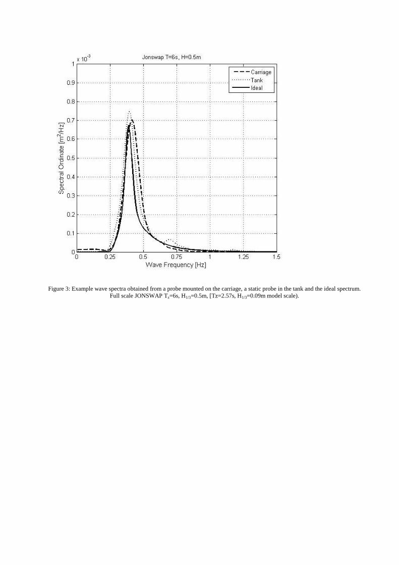
Figure 3: Example wave spectra obtained from a probe mounted on the carriage, a static probe in the tank and the ideal spectrum.

Full scale JONSWAP Tz=6s, H1/3=0.5m, [Tz=2.57s, H1/3=0.09m model scale).

Figure 4: Example heave motion time trace, run configuration 12

Figure 5: Example pitch motion time trace, run configuration 12

Figure 6 : Example CG acceleration time trace, run configuration 12

Figure 7: Example bow acceleration time trace, run configuration 12

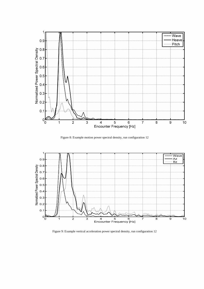
Figure 8: Example motion power spectral density, run configuration 12

Figure 9: Example vertical acceleration power spectral density, run configuration 12

Figure 10: Example distribution of wave heights, run configuration 12

Figure 11: Example distribution of heave minima, run configuration 12

Figure 12: Example distribution of heave maxima, run configuration 12

Figure 13: Example distribution of pitch maxima, run configuration 12

Figure 14: Example distribution of pitch minima, run configuration 12

Figure 15: Example distribution of vertical accelerations minima at LCG, run configuration 12

Figure 16: Example distribution of vertical acceleration minima at the bow, run configuration 12

Figure 17: Linear regression model of Cv and L/1/3 on RMS vertical accelerations at LCG [m/s2].

Figure 18: Linear regression model of Cv and L/1/3 on RMS vertical accelerations at the bow [m/s2].

Figure 19: Influence of steps on the RMS vertical accelerations

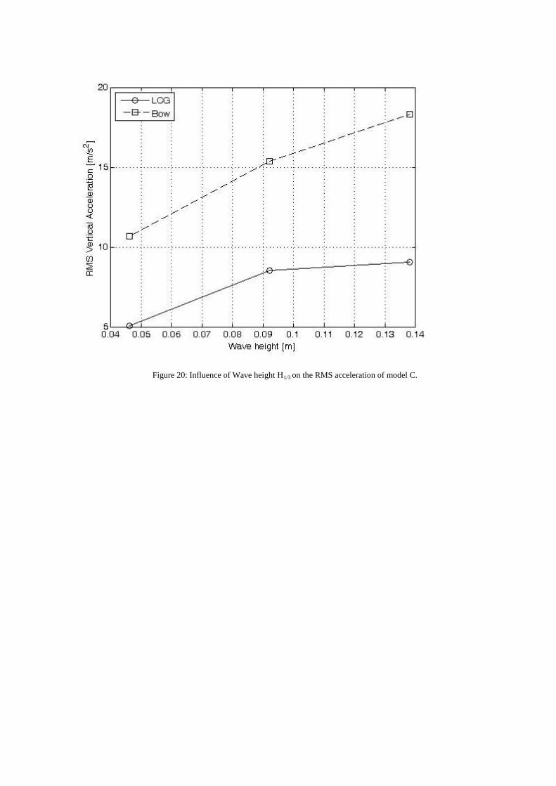
Figure 20: Influence of Wave height H1/3 on the RMS acceleration of model C.