characteristics of white spots in saturated wet snow

Characteristics of white spots in saturated wet snow

Takao KAMEDA,1 Yasuhiro HARADA,2 Shuhei TAKAHASHI1

1Snow and Ice Research Laboratory, Department of Civil and Environmental Engineering, Kitami Institute of Technology,Kitami, Hokkaido, Japan

E-mail: [email protected] Engineering Laboratory, Department of Computer Science, Kitami Institute of Technology, Kitami,

Hokkaido, Japan

ABSTRACT. Many curious white spots of 1–10 cm diameter were found on wet snow (�10mm thick)on the morning of 1 November 2009 in Kitami and Oketo in Hokkaido, Japan. At first glance, the whitespots appeared to be made of spherically gathered snow; however, they had actually been formed bythe scattering of sunlight over wet snow. Thin air bubbles enclosed in the wet snow caused a diffusereflection of sunlight and formed the white spots. We refer to this phenomenon as white spotted wetsnow. Although this type of snow has been briefly described previously, the formation process,meteorological conditions that lead to its formation, its vertical structure and the horizontaldistribution of the white spots are unknown. Our study addresses these issues. In addition, threeindependent methods (a nearest-neighbour method, Voronoi diagram and two-dimensional correlationfunction) demonstrate that the white spots are not randomly distributed but tend to be surrounded bysix other spots.

KEYWORDS: snow/ice surface processes

1. INTRODUCTIONMany curious white spots of 1–10 cm diameter were foundon wet snow (�10mm thick) on the morning of 1 November2009 in Kitami and Oketo in Hokkaido, Japan. We refer tothis phenomenon as ‘white spotted wet snow’. Most of thewhite spotted wet snow was observed on an asphalt pavedroad, but it was also observed on concrete and tilepavements, which are almost impermeable to water.

This phenomenon has been noted in Japan previously.Nohguchi (1984) wrote that ‘After snow deposition of 1 or2 cm in thickness and rain, snow with air bubbles willappear’ (translated from Japanese). He presented a photo-graph of white spotted wet snow, as did Hayashi (1985).Kominami and Yokoyama (2004) reported observations of‘white spotted wet snow’ at Jyoetsu, Niigata Prefecture, on7 March 2004. The Daily News in Niigata (local communitynewspaper published in Niigata district in Japan) published abeautiful picture of white spotted wet snow on 28 February2004, which was taken by Noriko Kawano on 25 February2004 at Joetsu, Niigata. All these reports describe obser-vations of white spotted wet snow. However, there havebeen no investigations of the formation process, meteoro-logical conditions that lead to its formation, its verticalstructure and the horizontal pattern of the white spots. Oneof the authors (S.T.) has lived in Kitami for more than 30 yearsbut had not seen this phenomenon previously.

This paper presents the characteristics of white spottedwetsnow observed in Kitami and Oketo on 1 November 2009.

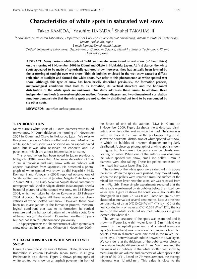
2. CHARACTERISTICS OF WHITE SPOTTED WETSNOWFigure 1 shows the study area of Kitami, Oketo, Bihoro andRubeshibe in eastern Hokkaido, Japan. Joetsu in NiigataPrefecture is also shown. Figure 2 shows photographs ofwhite spotted wet snow on an asphalt pavement in front of

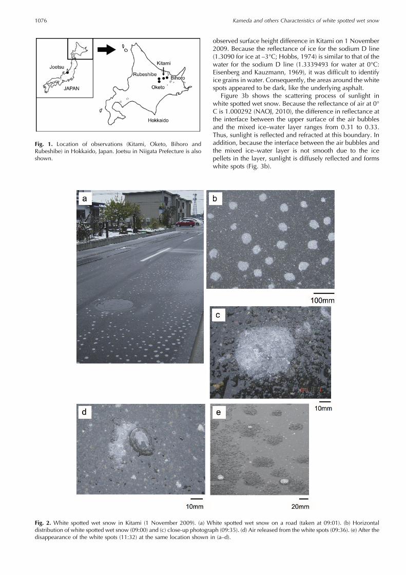
the house of one of the authors (T.K.) in Kitami on1 November 2009. Figure 2a shows the widespread distri-bution of white spotted wet snow on the road. The snow was5–10mm thick at the time of the photograph. Figure 2bshows the horizontal distribution of white spotted wet snow,in which air bubbles of �40mm diameter are regularlydistributed. A close-up photograph of a white spot is shownin Figure 2c. Transparent ice grains can be clearly seenfloating on water. When one of the authors was observingthe white spotted wet snow, small ice pellets 1mm indiameter were also falling. These ice pellets deposited onthe mixed ice–water layer (Fig. 2c).

The centres of the white spots were raised �1mm abovethe snow. When the spots were pushed, they moved easily.When the ice pellets were removed from the surface of themixed ice–water layer near the spots, air was released fromthem (Fig. 2d). These simple experiments revealed that thewhite spots were formed by air bubbles below themixed ice–water layer. Figure 2e shows the condition�3 hours after thephotograph in Figure 2d was taken. Some ice grains haveclustered at intervals of several centimetres. Because the heatconductivity of air at 0°C (0.024Wm–2K–1) is �1/20 of theheat conductivity of water at 0°C (0.561Wm–2K–1), the icegrains on the white spots did not melt, whereas ice grainslocated elsewhere did.

The vertical structure of the spots was examined and isshown in Figure 3a. A thin water layer (2–5mm thick) waspresent on the asphalt pavement, and a mixed ice–waterlayer (2–3mm thick) was present on the thin water layer. Icepellets 1mm in diameter were enclosed in the mixed ice–water layer. There was an air bubble between the two layers.We consider that the thickness of the bubbles was close tothe surface height difference of 1mm. We measured thethickness of air bubbles in the white spotted wet snow bymeasuring the air volume and diameter of white spots in thewinter of 2010/11. Based on 79 measurements, the averagethickness was 1.1�0.5mm. This value is close to the

Journal of Glaciology, Vol. 60, No. 224, 2014 doi: 10.3189/2014JoG13J201 1075

observed surface height difference in Kitami on 1 November2009. Because the reflectance of ice for the sodium D line(1.3090 for ice at –3°C; Hobbs, 1974) is similar to that of thewater for the sodium D line (1.3339493 for water at 0°C:Eisenberg and Kauzmann, 1969), it was difficult to identifyice grains in water. Consequently, the areas around the whitespots appeared to be dark, like the underlying asphalt.

Figure 3b shows the scattering process of sunlight inwhite spotted wet snow. Because the reflectance of air at 0°C is 1.000292 (NAOJ, 2010), the difference in reflectance atthe interface between the upper surface of the air bubblesand the mixed ice–water layer ranges from 0.31 to 0.33.Thus, sunlight is reflected and refracted at this boundary. Inaddition, because the interface between the air bubbles andthe mixed ice–water layer is not smooth due to the icepellets in the layer, sunlight is diffusely reflected and formswhite spots (Fig. 3b).

Fig. 1. Location of observations (Kitami, Oketo, Bihoro andRubeshibe) in Hokkaido, Japan. Joetsu in Niigata Prefecture is alsoshown.

Fig. 2. White spotted wet snow in Kitami (1 November 2009). (a) White spotted wet snow on a road (taken at 09:01). (b) Horizontaldistribution of white spotted wet snow (09:00) and (c) close-up photograph (09:35). (d) Air released from the white spots (09:36). (e) After thedisappearance of the white spots (11:32) at the same location shown in (a–d).

Kameda and others Characteristics of white spotted wet snow1076

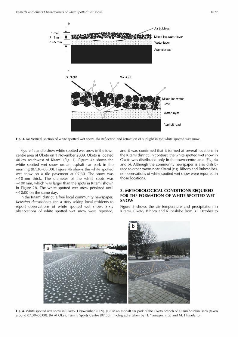
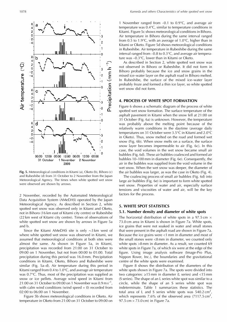
Figure 4a and b show white spotted wet snow in the towncentre area of Oketo on 1 November 2009. Oketo is located40 km southwest of Kitami (Fig. 1). Figure 4a shows thewhite spotted wet snow on an asphalt car park in themorning (07:30–08:00). Figure 4b shows the white spottedwet snow on a tile pavement at 07:30. The snow was�10mm thick. The diameter of the white spots was�100mm, which was larger than the spots in Kitami shownin Figure 2b. The white spotted wet snow persisted until�10:00 on the same day.

In the Kitami district, a free local community newspaper,Keizaino denshobato, ran a story asking local residents toreport observations of white spotted wet snow. Sixtyobservations of white spotted wet snow were reported,

and it was confirmed that it formed at several locations inthe Kitami district. In contrast, the white spotted wet snow inOketo was distributed only in the town centre area (Fig. 4aand b). Although the community newspaper is also distrib-uted to other towns near Kitami (e.g. Bihoro and Rubeshibe),no observations of white spotted wet snow were reported inthose locations.

3. METEOROLOGICAL CONDITIONS REQUIREDFOR THE FORMATION OF WHITE SPOTTED WETSNOWFigure 5 shows the air temperature and precipitation inKitami, Oketo, Bihoro and Rubeshibe from 31 October to

Fig. 3. (a) Vertical section of white spotted wet snow. (b) Reflection and refraction of sunlight in the white spotted wet snow.

Fig. 4. White spotted wet snow in Oketo (1 November 2009). (a) On an asphalt car park of the Oketo branch of Kitami Shinkin Bank (takenaround 07:30–08:00). (b) At Oketo Family Sports Centre (07:30). Photographs taken by H. Yamaguchi (a) and M. Hiwada (b).

Kameda and others Characteristics of white spotted wet snow 1077

2 November, recorded by the Automated MeteorologicalData Acquisition System (AMeDAS) operated by the JapanMeteorological Agency. As described in Section 2, whitespotted wet snow was observed only in Kitami and Oketo,not in Bihoro (16 km east of Kitami city centre) or Rubeshibe(22 km west of Kitami city centre). Times of observations ofwhite spotted wet snow are shown by arrows in Figure 5aand b.

Since the Kitami AMeDAS site is only �3 km west ofwhere white spotted wet snow was observed in Kitami, weassumed that meteorological conditions at both sites werealmost the same. As shown in Figure 5a, in Kitami,precipitation was recorded from 21:00 on 31 October to09:00 on 1 November, but not from 00:00 to 01:00. Totalprecipitation during this period was 16.0mm. Precipitationconditions in Kitami, Oketo, Bihoro and Rubeshibe weresimilar (Fig. 5a–d). Air temperature during this period inKitami ranged from 0.4 to 1.0°C, and average air temperaturewas 0.7°C. Thus, most of the precipitation was supplied assnow or ice pellets. Average wind speed in Kitami from21:00 on 31 October to 09:00 on 1 November was 0.9m s–1,with calm wind conditions (wind speed = 0) recorded from02:00 to 06:00 on 1 November.

Figure 5b shows meteorological conditions in Oketo. Airtemperature in Oketo from 21:00 on 31 October to 09:00 on

1 November ranged from –0.1 to 0.9°C, and average airtemperature was 0.4°C, similar to temperature conditions inKitami. Figure 5c showsmeteorological conditions in Bihoro.Air temperature in Bihoro during the same interval rangedfrom 0.5 to 1.9°C, with an average of 1.0°C, higher than inKitami or Oketo. Figure 5d shows meteorological conditionsin Rubeshibe. Air temperature in Rubeshibe during the sameinterval ranged from –0.8 to 0.3°C, and average air tempera-ture was –0.3°C, lower than in Kitami or Oketo.

As described in Section 2, white spotted wet snow wasnot observed in Bihoro or Rubeshibe. It did not form inBihoro probably because the ice and snow grains in themixed ice–water layer on the asphalt road in Bihoro melted.In Rubeshibe, the surface of the mixed ice–water layerprobably froze and formed a thin ice layer, so white spottedwet snow did not form.

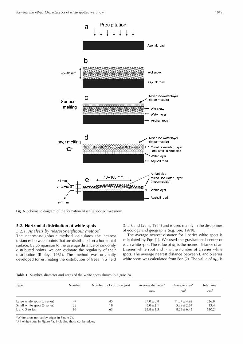
4. PROCESS OF WHITE SPOT FORMATIONFigure 6 shows a schematic diagram of the process of whitespotted wet snow formation. The surface temperature of theasphalt pavement in Kitami when the snow fell at 21:00 on31 October (Fig. 6a) is unknown. However, the temperaturewas probably above the melting point because of therelatively warm conditions in the daytime (average dailytemperatures on 31 October were 3.5°C in Kitami and 2.0°Cin Oketo). Thus, snow melted on the road and formed wetsnow (Fig. 6b). When snow melts on a surface, the surfacesnow layer becomes impermeable to air (Fig. 6c). In thiscase, the void volumes in the wet snow became small airbubbles (Fig. 6d). These air bubbles coalesced and formed airbubbles 10–100mm in diameter (Fig. 6e). Consequently, theair in the bubbles was supplied from the void volume in thewet snow. When the wet snow was deeper, the diameter ofthe air bubbles was larger, as was the case in Oketo (Fig. 4).

The coalescing process of small air bubbles (Fig. 6d) intolarge air bubbles (Fig. 6e) is important to form white spottedwet snow. Properties of water and air, especially surfacetensions and viscosities of water and air, will be the keyfactors for the process.

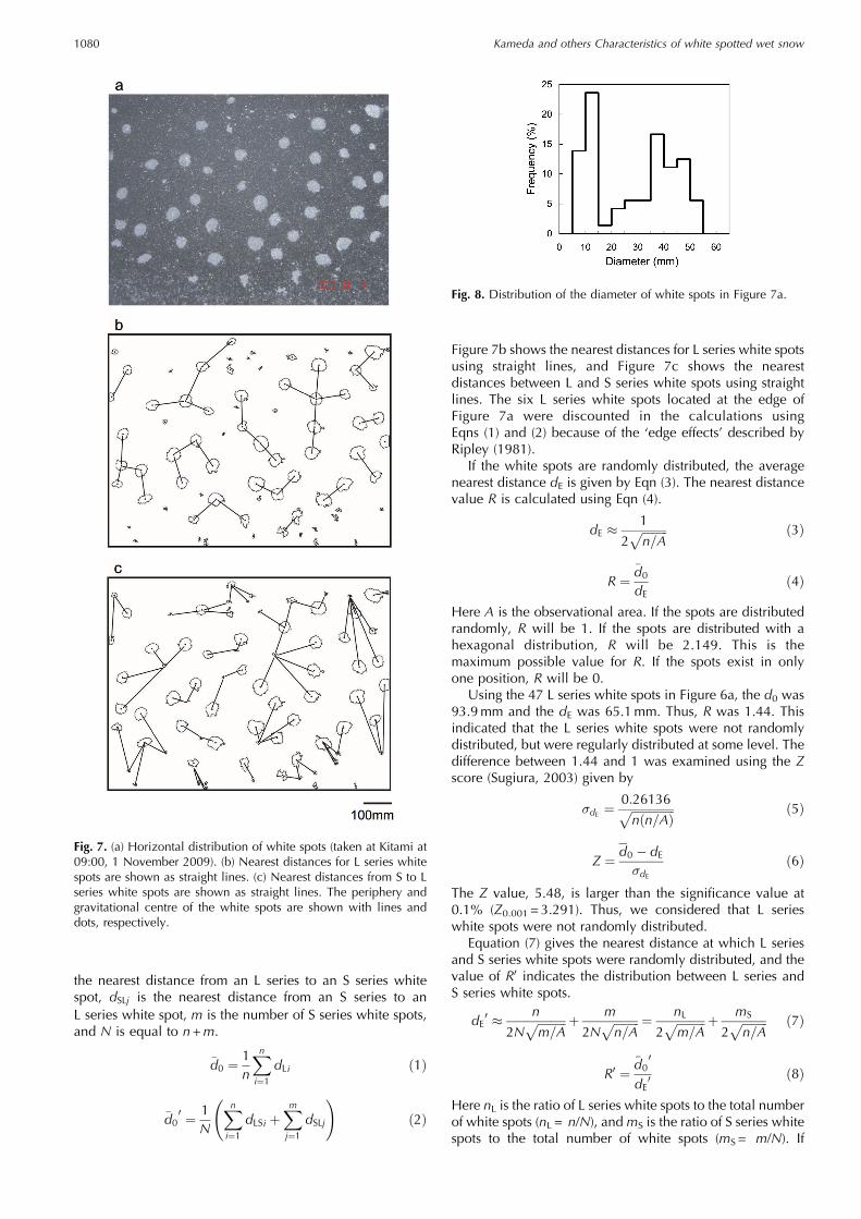
5. WHITE SPOT STATISTICS5.1. Number density and diameter of white spotsThe horizontal distribution of white spots in a 97.5 cm �73.0 cm area in Kitami is shown in Figure 7a. White spots,ice grains that were not soaked in water and small stonesthat were present in the asphalt road are shown in Figure 7a.Because the ice grains were <1mm in diameter and most ofthe small stones were <8mm in diameter, we counted onlywhite spots >8mm in diameter. As a result, we counted 69white spots in Figure 7a, of which six were at the edge of thefigure. Using image analysis software (Image-Pro Plus,Nippon Rover, Inc.), the boundaries and the gravitationalcentre of the white spots were examined.

Figure 8 shows the distribution of the diameters of thewhite spots shown in Figure 7a. The spots were divided intotwo categories: ≥15mm in diameter (L series) and <15mm(S series). The shape of an L series white spot was similar to acircle, while the shape of an S series white spot wasindeterminate. Table 1 summarizes these statistics. Thetotal area of L and S series white spots was 540.2 cm2,which represents 7.6% of the observed area (7117.5 cm2,97.5 cm� 73.0 cm) in Figure 7a.

Fig. 5.Meteorological conditions in Kitami (a), Oketo (b), Bihoro (c)and Rubeshibe (d) from 31 October to 2 November from the JapanMeteorological Agency. The times when white spotted wet snowwere observed are shown by arrows.


5.2. Horizontal distribution of white spots5.2.1. Analysis by nearest-neighbour methodThe nearest-neighbour method calculates the nearestdistances between points that are distributed on a horizontalsurface. By comparison to the average distance of randomlydistributed points, we can estimate the regularity of theirdistribution (Ripley, 1981). The method was originallydeveloped for estimating the distribution of trees in a field

(Clark and Evans, 1954) and is used mainly in the disciplinesof ecology and geography (e.g. Lee, 1979).

The average nearest distance for L series white spots iscalculated by Eqn (1). We used the gravitational centre ofeach white spot. The value of dLi is the nearest distance of anL series white spot and n is the number of L series whitespots. The average nearest distance between L and S serieswhite spots was calculated from Eqn (2). The value of dLSi is

Fig. 6. Schematic diagram of the formation of white spotted wet snow.

Table 1. Number, diameter and areas of the white spots shown in Figure 7a

Type Number Number (not cut by edges) Average diameter* Average area* Total area†

mm cm2 cm2

Large white spots (L series) 47 45 37.0� 8.8 11.37�4.92 526.8

Small white spots (S series) 22 18 8.0� 2.1 5.39�2.87 13.4

L and S series 69 63 28.8� 1.5 8.28�6.45 540.2

*White spots not cut by edges in Figure 7a.†All white spots in Figure 7a, including those cut by edges.


the nearest distance from an L series to an S series whitespot, dSLj is the nearest distance from an S series to anL series white spot, m is the number of S series white spots,and N is equal to n+m.

�d0 ¼1n

Xn

i¼1dL i ð1Þ

�d00¼

1N

Xn

i¼1dLSi þ

Xm

j¼1dSLj

!

ð2Þ

Figure 7b shows the nearest distances for L series white spotsusing straight lines, and Figure 7c shows the nearestdistances between L and S series white spots using straightlines. The six L series white spots located at the edge ofFigure 7a were discounted in the calculations usingEqns (1) and (2) because of the ‘edge effects’ described byRipley (1981).

If the white spots are randomly distributed, the averagenearest distance dE is given by Eqn (3). The nearest distancevalue R is calculated using Eqn (4).

dE �1

2ffiffiffiffiffiffiffiffiffin=A

p ð3Þ

R ¼�d0dE

ð4Þ

Here A is the observational area. If the spots are distributedrandomly, R will be 1. If the spots are distributed with ahexagonal distribution, R will be 2.149. This is themaximum possible value for R. If the spots exist in onlyone position, R will be 0.

Using the 47 L series white spots in Figure 6a, the d0 was93.9mm and the dE was 65.1mm. Thus, R was 1.44. Thisindicated that the L series white spots were not randomlydistributed, but were regularly distributed at some level. Thedifference between 1.44 and 1 was examined using the Zscore (Sugiura, 2003) given by

�dE ¼0:26136ffiffiffiffiffiffiffiffiffiffiffiffiffiffiffinðn=AÞ

p ð5Þ

Z ¼d0 � dE�dE

ð6Þ

The Z value, 5.48, is larger than the significance value at0.1% (Z0.001 = 3.291). Thus, we considered that L serieswhite spots were not randomly distributed.

Equation (7) gives the nearest distance at which L seriesand S series white spots were randomly distributed, and thevalue of R0 indicates the distribution between L series andS series white spots.

dE0 �n

2Nffiffiffiffiffiffiffiffiffiffim=A

p þm

2Nffiffiffiffiffiffiffiffiffin=A

p ¼nL

2ffiffiffiffiffiffiffiffiffiffim=A

p þmS

2ffiffiffiffiffiffiffiffiffin=A

p ð7Þ

R0 ¼�d00

dE0ð8Þ

Here nL is the ratio of L series white spots to the total numberof white spots (nL = n/N), andmS is the ratio of S series whitespots to the total number of white spots (mS = m/N). If

Fig. 7. (a) Horizontal distribution of white spots (taken at Kitami at09:00, 1 November 2009). (b) Nearest distances for L series whitespots are shown as straight lines. (c) Nearest distances from S to Lseries white spots are shown as straight lines. The periphery andgravitational centre of the white spots are shown with lines anddots, respectively.

Fig. 8. Distribution of the diameter of white spots in Figure 7a.


L series white spots and S series white spots are randomlydistributed, R0 will be 1. If L series white spots and S serieswhite spots are distributed at only one point, R0 will be 0. Ifall L series white spots are located on S series white spots, R0will be 0.

Using Eqns (2) and (7), d00 was 98.2mm and dE was75.0mm, and thus R0 was 1.31. This means that S serieswhite spots were not randomly distributed. In other words,S series white spots were distributed close to L series whitespots at some level. The difference between 1.31 and 1 wasexamined using the Z score (Sugiura, 2003) given by

�dE 0 ¼

ffiffiffiffiffiffiffiffiffiffi�2dE0

N

s

ð9Þ

�2dE0 ¼

nnLðn=AÞð4 � �nLÞ þmSðm=AÞð4 � �mSÞ

� 2�nLmS ðn=AÞðm=AÞ½ �1=2o=4�ðn=AÞðm=AÞ

ð10Þ

Z ¼d00� dE0

�dE 0ð11Þ

The Z value comes to 5.14, larger than the significancevalue at 0.1% (Z0.001 = 3.291). Thus, we considered that Sseries white spots were not randomly distributed.

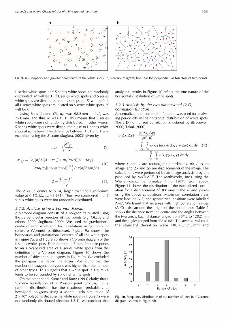
5.2.2. Analysis using a Voronoi diagramA Voronoi diagram consists of a polygon calculated usingthe perpendicular bisectors of two points (e.g. Okabe andothers, 2000; Sugihara, 2009). We used the gravitationalcentre of each white spot for calculations using computersoftware (Voronoi partition.exe). Figure 9a shows theboundaries and gravitational centres of all the white spotsin Figure 7a, and Figure 9b shows a Voronoi diagram of theL series white spots. Each domain in Figure 9b correspondsto an air-captured area of L series white spots from thedefinition of a Voronoi diagram. Figure 10 shows thenumber of sides in the polygons in Figure 9b. We excludedthe polygons that faced the edges. We found that thenumber of hexagonal polygons was higher than the numberof other types. This suggests that a white spot in Figure 7atends to be surrounded by six other white spots.

On the other hand, Kumar and Kurtz (1993) clarify that aVoronoi tessellation of a Poisson point process, i.e. arandom distribution, has the maximum probability athexagonal polygons using a Monte Carlo simulation of2�106 polygons. Because the white spots in Figure 7a werenot randomly distributed (Section 5.2.1), we consider that

analytical results in Figure 10 reflect the true nature of thehorizontal distribution of white spots.

5.2.3 Analysis by the two-dimensional (2-D)correlation functionA normalized autocorrelation function was used for analys-ing periodicity in the horizontal distribution of white spots.The 2-D normalized correlation is defined by (Bracewell,2000; Takai, 2000)

~’ð�x,�yÞ ¼’ð�x,�yÞ’ð0, 0Þ

¼

R1

� 1

R1

� 1

uðx, yÞuðx þ�x, yþ�yÞ dx dy

R1

� 1

R1

� 1

uðx, yÞuðx, yÞ dx dy

ð12Þ

where x and y are rectangular coordinates, u(x,y) is animage, and �x and �y are displacements of the image. Thecalculations were performed by an image analysis programproduced by MATLAB® (The MathWorks, Inc.) using theWiener–Khintchine formulae (Hino, 1977; Takai, 2000).Figure 11 shows the distribution of the normalized correl-ation for a displacement of 300mm in the x- and y-axesusing the above calculations. Maximum correlation areaswere labelled A–E, and symmetrical positions were labelledA0–E0. We found that six areas with high correlation values(A–C) exist around the origin of the coordinates. Table 2shows the distance from the centre and the angles betweenthe two areas. Each distance ranged from 87.2 to 120.2mmand the angles ranged from 43° to 68°. The average values�the standard deviation were 106.7�17.3 mm and

Fig. 9. (a) Periphery and gravitational centre of the white spots. (b) Voronoi diagram; lines are the perpendicular bisectors of two points.

Fig. 10. Frequency distribution of the number of lines in a Voronoidiagram, shown in Figure 9b.


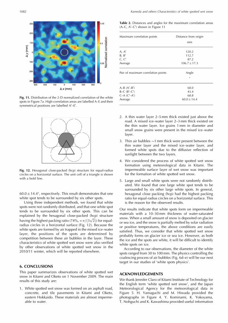
60.0�14.4°, respectively. This result demonstrates that onewhite spot tends to be surrounded by six other spots.

Using three independent methods, we found that whitespots were not randomly distributed, and that one white spottends to be surrounded by six other spots. This can beexplained by the hexagonal close-packed (hcp) structurehaving the highest packing ratio (74%, =�=ð3

ffiffiffi2pÞ) for equal-

radius circles in a horizontal surface (Fig. 12). Because thewhite spots are formed by air trapped in the mixed ice–waterlayer, the positions of the spots are determined bycompetition between these air bubbles in the layer. Thesecharacteristics of white spotted wet snow were also verifiedby other observations of white spotted wet snow in the2010/11 winter, which will be reported elsewhere.

6. CONCLUSIONSThis paper summarizes observations of white spotted wetsnow in Kitami and Oketo on 1 November 2009. The mainresults of this study are:

1. White spotted wet snow was formed on an asphalt road,concrete, and tile pavements in Kitami and Oketo,eastern Hokkaido. These materials are almost imperme-able to water.

2. A thin water layer 2–5mm thick existed just above theroad. A mixed ice–water layer 2–3mm thick existed onthe thin water layer. Ice grains 1mm in diameter andsmall snow grains were present in the mixed ice–waterlayer.

3. Thin air bubbles �1mm thick were present between thethin water layer and the mixed ice–water layer, andformed white spots due to the diffusive reflection ofsunlight between the two layers.

4. We considered the process of white spotted wet snowformation using meteorological data in Kitami. Theimpermeable surface layer of wet snow was importantfor the formation of white spotted wet snow.

5. Large and small white spots were not randomly distrib-uted. We found that one large white spot tends to besurrounded by six other large white spots. In general,hexagonal close packing (hcp) had the highest packingratio for equal-radius circles on a horizontal surface. Thisis the reason for the observed results.

Our results indicate that white spots form on impermeablematerials with a 10–30mm thickness of water-saturatedsnow. When a small amount of snow is deposited on glacieror sea ice, and the snow is partially melted by solar radiationor positive temperatures, the above conditions are easilysatisfied. Thus, we consider that white spotted wet snowprobably forms on glacier ice or sea ice. However, as boththe ice and the spots are white, it will be difficult to identifywhite spots on ice.

According to our observations, the diameter of the whitespots ranged from 30 to 100mm. The physics controlling thecoalescing process of air bubbles (Fig. 6d–e) will be our nexttarget in our studies of ‘white spots physics’.

ACKNOWLEDGEMENTSWe thank Jennifer Claro of Kitami Institute of Technology forthe English term ‘white spotted wet snow’, and the JapanMeteorological Agency for the meteorological data inFigure 5. H. Yamaguchi and M. Hiwada provided thephotographs in Figure 4. Y. Kominami, K. Yokoyama,T. Nohguchi and K. Kawashima provided useful information

Table 2. Distances and angles for the maximum correlation areas(A–C, A0–C0) shown in Figure 11

Maximum correlation points Distance from origin

mm

A, A0 120.2

B, B0 112.7

C, C0 87.2

Average 106.7�17.3

Pair of maximum correlation points Angle

°

A–B (A0–B0) 68.0

B–C (B0–C0) 43.4

C–A (C0–A0) 68.8

Average 60.0�14.4

Fig. 12. Hexagonal close-packed (hcp) structure for equal-radiuscircles on a horizontal surface. The unit cell of a triangle is shownwith a bold line.

Fig. 11. Distribution of the 2-D normalized correlation of the whitespots in Figure 7a. High-correlation areas are labelled A–E and theirsymmetrical positions are labelled A0–E0.


on the white spotted wet snow in the Niigata district.Y. Sadahiro and Y. Kurata informed us of the literaturerelating to point pattern analyses. K. Higuchi providedthoughtful advice. M. Hanaoka, a journalist for Keizainodenshobato, contributed to the collection of the obser-vations in the Kitami district by publishing an article entitled‘To readers, information needed on white spot phenomena’in his daily newspaper. T. Murawaki helped with thecalculations used for Figure 11. We also thank anonymousreviewers and the scientific editor, Perry Bartelt, forconstructive comments on an earlier version of this paper.

REFERENCESBracewell RN (2000) The Fourier Transform and its applications,

3rd edn. McGraw Hill, Boston, MAClark PJ and Evans FC (1954) Distance to nearest neighbor as a

measure of spatial relationships in populations. Ecology, 35(4),445–453 (doi: 10.2307/1931034)

Eisenberg D and Kauzmann W (1969) The structure and propertiesof water. Oxford University Press, Oxford [reprinted 2005]

Hayashi A (1985) Uonuma village, words relating to snow. OogiyaPublishing, Tokyo [in Japanese]

Hino M (1977) Spectral analysis. Asakura Shoten, Tokyo [inJapanese]

Hobbs PV (1974) Ice physics. Clarendon Press, OxfordKominami Y and Yokoyama K (2004) The air bubbles in the thin

soaked snow pack. In Preprints of the Annual Conference 2004,Japanese Society of Snow and Ice, 27–30 September, Hikone,Shiga. Japanese Society of Snow and Ice, Tokyo, P2–38 [inJapanese]

Kumar S and Kurtz SK (1993) Properties of a two-dimensionalPoisson–Voronoi tessellation: a Monte-Carlo study. Mater.Charact., 31(1), 55–68 (doi: 10.1016/1044-5803(93)90045-W)

Lee Y (1979) A nearest-neighbor spatial-association measure for theanalysis of firm interdependence. Environ. Plan., 11, 169–176

National Astronomical Observatory of Japan (NAOJ) (2010)Chronological scientific tables. Maruzen, Tokyo

Nohguchi Y (1984) Formation of dimple-pattern on snow. 1. Rep.Nat. Res. Cent. Disaster Prev., 33, 237–254 [in Japanese withEnglish summary]

Okabe A, Boots B, Sugihara K and Chiu SN (2000) Spatialtessellations: concepts and applications of Voronoi diagrams,2nd edn. Wiley, Chichester

Ripley BD (1981) Spatial statistics. Wiley, Hoboken, NJSugihara K (2009)Mathematical models of territories: introduction tomathematical engineering through Voronoi diagrams. KyoritsuShuppan, Tokyo [in Japanese]

Sugiura Y (2003) Geographical spatial analyses. (Human Geog-raphy 3) Asakura, Tokyo [in Japanese]

Takai N (2000) Introduction to MATLAB for signal and imageprocesses. Kougaku-sha, Tokyo [in Japanese]

MS received 17 October 2013 and accepted in revised form 31 July 2014


characteristics of white spots in saturated wet snow

Documents