1

a

Documentation March 2012 Using charts and graphs in Excel is an excellent way to communicate the meaning of a group or series of numbers in a simple, visual way that makes more sense to most people than looking at raw data. Charts and graphs can be used to see how much your gas bill has changed over a 12 month period, which salespeople are bringing in the most money, which flavor of popsicle is most popular, and other numerical comparisons. Any range of data input in Excel can be translated into a chart or graph, which can especially useful when giving presentations in work situations. The concept behind charts and graphs is that a picture is worth a thousand words; today we will learn how to draw those pictures with Excel. Types of Charts Excel offers a variety of charts and most have several subtypes associated with them. Be sure to choose the correct chart for the data in the spreadsheet.

• Area • Bar • Column • Line • Pie • XY (Scattergram)

The information in this table was obtained from Microsoft Excel Help. Area Chart Area Charts show individual volume changes over time in relation to total volume or the size of total change over a period of time. For example, data that represents profit over time can be plotted in an area chart to emphasize the total profit. Area Chart Subtypes:

• 2d and 3D Area graphs • Stacked area and stacked area in 3-D • 100% stacked area and 100% stacked area in 3-D

Charts and Graphs

in Excel 2010

2

2-D area and 3-D area charts display the trend of values over time

or other category data. 3-D area charts use three axes (horizontal, vertical, and depth) that can be modified. As a rule, consider using a line chart instead of a nonstacked area chart, because data from one series can be obscured by data from another series.

Stacked area and stacked area in 3-D – Stacked area charts display the trend of the contribution of each value over time or other category data. The 3-D version is displayed in the same way but uses a 3-D perspective. A 3-D perspective is not a true 3-D chart; a third value axis (depth axis) is not used.

100% stacked area and 100% stacked area in 3-D – 100% stacked area charts display the trend of the percentage that each value contributes over time or other category data. The 3-D version is displayed in the same way but uses a 3-D perspective. A 3-D perspective is not a true 3-D chart; a third value axis (depth axis) is not used.

Bar Chart Bar Charts compare different object levels over time using a horizontal format that arranges data in columns or rows on a worksheet. Bar charts illustrate comparisons among individual items. Bar charts subtypes:

• Clustered bar and clustered bar in 3-D • Stacked bar and stacked bar in 3-D • 100% stacked bar and 100% stacked bar in 3-D • Horizontal cylinder, cone, and pyramid

Clustered bar and clustered bar in 3-D – Clustered bar charts

compare values across categories. The categories are typically organized along the vertical axis and the values along the horizontal axis. The 3-D version displays the horizontal rectangles in 3-D format; it does not display the data on three axes.

Stacked bar and stacked bar in 3-D – Stacked bar charts show the relationship of individual items to the whole. The 3-D version displays the horizontal rectangles in 3-D format; it does not display the data on three axes.

100% stacked bar and 100% stacked bar in 3-D charts compare the percentage that each value contributes to a total across categories. A 100% stacked bar in 3-D chart displays the horizontal rectangles in 3-D format; it does not display the data on three axes.

Horizontal cylinder, cone, and pyramid charts are available in the same clustered, stacked, and 100% stacked chart types provided for rectangular bar charts. They show and compare data the same way. Instead, these chart types display cylinder, cone, and pyramid shapes.

3

Column Graph Column Graphs compare different object levels over time using a vertical format. Data that is arranged in columns or rows on a worksheet can be plotted in a column chart. Column charts are useful for showing data changes over a period of time or for illustrating comparisons among items. Categories are typically organized along the horizontal axis and values along the vertical axis. Column charts subtypes:

• Clustered column and clustered column in 3-D • Stacked column and stacked column in 3-D • 100% stacked column and 100% stacked column in 3-D • 3-D column Charts • Cylinder, cone, and pyramid

Clustered column and clustered column in 3-D – See the

description for Cluster Bar and Clustered bar in 3-D.

Stacked column and stacked column in 3-D – See the description for Stacked bar and Stacked bar in 3-D.

100% stacked column and 100% stacked column in 3-D – See the description for 100% stacked Bar and 100% stacked bar in 3-D.

3-D column Charts – 3D column charts are used to compare data across categories and series equally, because this chart type shows categories along both the horizontal axis and the depth axis whereas the vertical axis displays the values.

Cylinder, cone, and pyramid – See the previous description for cylinder, cone, and pyramid charts.

4

Line Chart Line Charts compares a trend over even time intervals. Line charts subtypes:

• Line and line with markers • Stacked line and stacked line with markers • 100% stacked line and 100% stacked line with markers • 3-D Line

Line and line with markers charts indicate individual data values or are useful to show trends over time or ordered categories, especially when there are many data points and the order in which they are presented is important. If there are many categories or the values are approximate, use a line chart without markers.

Stacked line and stacked line with markers charts are used to indicate individual data values and to show the trend of the contribution of each value over time or ordered categories.

100% stacked line and 100% stacked line with markers are useful to show the trend of the percentage each value contributes over time or ordered categories. If there are many categories or the values are approximate, use a 100% stacked line chart without markers.

3-D line – 3-D line charts show each row or column of data as a 3-D ribbon. A 3-D line chart has horizontal, vertical, and depth axes that you can modify.

Pie Chart Pie Charts compare sizes of pieces as part of a whole. Since Pie charts represent a percentage of a whole, only one row or one column of a worksheet can be used. Pie Chart Sub-types:

• Pie and pie in 3-D • Pie of pie and bar of pie • Exploded pie and exploded pie in 3-D

Pie and pie in 3-D --- Pie charts display the contribution of each value

to a total in a 2-D or 3-D format. Slices of a pie chart can be pulled out manually to emphasize the slices.

5

Pie of pie and bar of pie charts display pie charts with user-defined values that are extracted from the main pie chart and combined into a secondary pie chart or into a stacked bar chart. These chart types are useful for making small slices in the main pie chart easier to distinguish.

Exploded pie and exploded pie in 3-D – Exploded pie charts display the contribution of each value to a total while emphasizing individual values. Exploded pie charts can be displayed in 3-D. The pie explosion settings can be changed for all slices and individual slices, but the slices of an exploded pie cannot be moved manually.

XY (Scatter) Chart XY (scatter) Charts compares trends over uneven time intervals; they are used in scientific and engineering disciplines for trend-spotting and extrapolation. XY (Scatter ) Chart Sub-types:

• Scatter with only markers • Scatter with smooth lines and scatter with smooth lines

and markers

Scatter with only markers charts compare pairs of values. Use a scatter chart with data markers but without lines when using many data points and connecting lines would make the data more difficult to read. Use this chart type when it is not necessary to show connectivity of the data points.

Scatter with smooth lines and scatter with smooth lines and markers charts display a smooth curve that connects the data points. Smooth lines can be displayed with or without markers. Use a smooth line without markers if there are many data points.

Scatter with straight lines and scatter with straight lines and markers charts display straight connecting lines between data points. Straight lines can be displayed with or without markers.

Other Chart Types

• Stock Charts • Surface Charts • Donut Charts • Bubble Charts • Radar Charts

6

Opening an Excel Document

1. Open Excel

2. Open the file excel_practice_file.xls located in the My Documents (or Documents) folder on the computer

3. If necessary, click the yellow Enable Editing button at the top of the Excel window

Navigate to the worksheet named romances, which lists the date for the number of romance books circulated by each branch of the Heights Library System for a one-week period. The days as well as the branches can be compared using different charts. The data on this sheet is used to create the charts in the following sections. Column Charts

1. Select columns A, B, C, D and E in rows, 3, 4 and 5

2. Go to the Insert tab � Charts group �

Column command

3. Choose the first option under the heading 2-D Column

The chart appears on the same sheet on which the data is located. Often, it appears on top of some of the data. To move the chart:

1. Click the edge of the window

2. When the 4-headed arrow appears, hold down the left mouse button and drag the chart.

7

Chart Tools Contextual Tabs When a chart is inserted and selected, three contextual sub tabs appear on the right end of the Ribbon:

1. Chart Tools - Design 2. Chart Tools - Layout 3. Chart Tools - Format

NOTE: The Chart Tools contextual tabs only appear when the chart is selected. Chart Tools Design Sub Tab The Design sub tab provides tools for changing the look and feel of the chart. To avoid a lot of manual formatting, Microsoft Office Excel provides a variety of useful predefined quick layouts and styles.

The Chart Layouts group provides options for changing the layout of the chart. The Chart Styles group can be used to quickly choose new colors for the chart.

1. Click the chart to be formatted

2. Go to the Chart Tools Design tab � Chart Styles group � Chart Styles more arrow to open the Chart Styles gallery

3. Click the desired color style, such as green style 21

4. Go to the Chart Tools Design tab � Chart Styles group � Chart Layouts more arrow to see all available layouts

5. Click the desired layout, such as layout 10

8

Switching the Row and Column To the left of the Chart Layouts group are the Data and Type groups. Using the Data group, it is possible to switch rows and columns or choose different data. Switching rows and columns can be useful in comparing the data in a different way.

1. If necessary, click the chart to be formatted

2. Go to the Design sub tab � Data group � Switch Row/column command

NOTE: Some charts do not display correctly with the columns and rows swapped.

Moving the Chart to another Worksheet Excel 2010 offers two ways for a chart to be moved to worksheet:

• Create a new sheet for the chart • Move the chart to another sheet in the workbook

1. If necessary, click the chart to be moved 2. Go to the Design sub tab � Location group � Move Chart command

• To move the chart to a new blank sheet, choose the New sheet bullet and click OK • To move the chart to a worksheet that already exists, choose the Object in bullet, click the down

arrow at the right end of the box and select the desired worksheet

Chart Tools Layout Sub Tab Use the Layout sub tab to:

• insert pictures, shapes, and text boxes • edit the chart’s labels, axes, and background • manually change the Chart layout

9

Adding a Title A title can be added to the chart through the Layout sub tab � Labels group � Chart Title command. Choose a location for the title, select the words Chart Title, and type in a new title. Adding a Text Box

1. Click the chart to be formatted 2. Go to the Layout sub tab � Insert group � Text Box command 3. Click inside the chart where you want the box to appear; a text box is

inserted

• Text boxes can be resized using the resizing circles on the border. • Text boxes can be moved to another location within the chart area by clicking and dragging. • The small green circle at the top rotates the text box to a new angle.

Adding Data Labels

1. Click the chart to be formatted 2. Go to the Layout sub tab � Labels group � Data

Labels command 3. Choose where the data labels should appear, such as

Inside End

10

Adding an Axis Title Axis titles can be added for either or both of the primary axes through the Layout sub tab � Labels group � Axis Titles command; several title options appear. Adding Gridline and Axes In the Layout sub tab � Axes group are options to edit the axes and gridlines (for example, adding more horizontal or vertical lines to show additional detail on the chart). Chart Tools Format Sub Tab

The Format tab contains commands for changing the fill, outline and shape of the plot area, in addition to the color, style, outline, and fill of text within the chart.

The Current Selection group is helpful in selecting specific parts of the chart to edit. It keeps track of what is currently selected and offers a myriad of formatting options such as fills, border and line color, border and line style, shadowing, and 3-D formatting. Formatting a Selection 1. Click the down arrow in the

Current Selection box 2. Select the desired section,

such as Plot Area 3. Click on Format Selection;

the appropriate dialog box opens (Format Plot Area)

4. Choose the Gradient fill bullet 5. Click the Preset colors arrow

and choose a gradient 6. Click Close NOTE: Not all formatting options are available for all parts of a chart—the dialog box changes to reflect options that are available for the current selection. The Shape Styles group offers commands for controlling the shape around a part of the graph, including the fill and outline color and various effects for the shape (such as shadow, glow, bevel, reflection, and 3-D rotation). The WordArt Styles group provides WordArt options. Change the color and style of lettering, add borders or fills, and apply different effects. NOTE: Not all options are available for every chart type. If a command is grayed out, it is not available for the selected chart.

11

Line Charts Let’s compare circulation at Coventry and Main using a line chart. 1. If necessary, go to the romances

worksheet

2. Select column A and B rows 3 through 10

3. To select a noncontiguous column, hold down the Ctrl key on the keyboard and select column D, rows 3 through 10

4. Go to the Insert tab � Charts group � Line command

5. Choose the first option in the second

row of the drop-down menu, Line with Markers A line chart with markers appears.

Changing Chart Colors Charts can be customized by changing the colors of one or more elements. NOTE: Changing a color on the chart is automatically reflected in the chart key. 1. Select the Main line on the chart

2. Go to the Format sub tab � Current Selection group � Format Selection

command; the Format Data Series dialog box opens, where the color, style, and many other elements of each piece of the chart can be changed

12

3. Click Marker Fill on the left side box

4. Click the Solid fill bullet in the Marker Fill section on the right

5. Click the Color arrow and select the dark red color

6. Click Close

NOTE: In a line chart, fill colors must be chosen for the marker and the line separately.

Pie Charts A pie chart is used to compare the input of various entities to a total. For example: comparing the percentages of branch contributions to the total circulation on a particular day.

1. If necessary, go to the romances worksheet

2. Select the Saturday data including the labels for row 10 (columns A through E)

3. Hold down the Ctrl key and select the labels in row 3 (columns A through E)

4. Go to the Insert tab � Charts group � Pie command

13

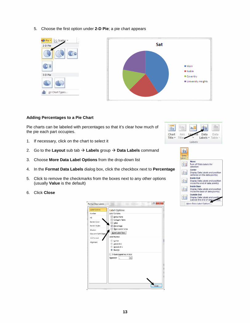
5. Choose the first option under 2-D Pie; a pie chart appears

Adding Percentages to a Pie Chart Pie charts can be labeled with percentages so that it’s clear how much of the pie each part occupies. 1. If necessary, click on the chart to select it

2. Go to the Layout sub tab � Labels group � Data Labels command

3. Choose More Data Label Options from the drop-down list

4. In the Format Data Labels dialog box, click the checkbox next to Percentage

5. Click to remove the checkmarks from the boxes next to any other options

(usually Value is the default) 6. Click Close

14

Tweaking a Chart Sometimes a chart needs to be tweaked to get the desired look. Following is a common problem that arises:

1. Go to the genre circ worksheet

2. Select cells A2 to C10

3. Go to the Insert tab � Column Chart

4. Choose the first chart The chart is treating the column containing the years as part of the data to be plotted rather than as labels for the horizontal axis.

To remedy this issue:

1. Go to the Chart Tools Design sub tab � Data group � Select Data command

2. In the Select Data Source dialog box, click on the series name Year in the box on the left

3. Click the Remove button in the Legend Entries section

4. In the Horizontal (Category) Axis Labels box on the right, click the Edit button

15

5. When the Axis Labels dialog box appears, select cells A3 to A10 on the spreadsheet

6. Click OK in the Axis Labels dialog box

7. The Select Data Source dialog box should now look like this:

8. Click OK to see the corrected chart; the Year column is gone and each year is now listed as a label

along the horizontal axis

16

The One-Click Chart To create a chart with just one click, select the data to be included in the chart and hit the F11 key on the keyboard; the chart should appear as a new sheet in the workbook. Try it using the romances sheet:

1. Select rows 3 through 10, columns A through E 2. Press the F11 key on the keyboard; the chart is created on a new page labeled Chart1

NOTE: If a Chart1 sheet already exists, the new chart is named by the next available number.

Practice Exercises

1. Add a new sheet to the workbook

2. Create a spreadsheet for the following data

regarding how many popsicles were sold over the summer months

June July August Grape 229 380 269

Cherry 380 430 501

Banana 120 487 643

Orange 256 400 520

3. Create a chart that shows the changes in popularity of popsicle flavors over the 3-month period.

NOTE: Line charts are useful for showing change over time.

4. Create a chart that shows which flavor sold the most overall in the 3-month period. NOTE: Stacked bar charts are useful for showing the relationship of individual items to the whole.

17

5. Create a chart that shows the percentages of different flavors sold during the month of June. NOTE: Pie charts are useful for comparing percentages of a whole.

6. Change the style and/or colors on one or more of the charts.