chemical process alternatives for radioactive waste 2012 yer...fiu-arc-2013-800000393-04b-213...
TRANSCRIPT

YEAR END TECHNICAL REPORT May 18, 2012 to August 17, 2013
Chemical Process Alternatives for Radioactive Waste
Submitted on August 17, 2013
Principal Investigators:
Leonel E. Lagos, Ph.D., PMP® David Roelant, Ph.D.
Florida International University Collaborators:
Dwayne McDaniel, Ph.D., P.E. (Project Manager) Jose Varona, M.S.
Amer Awwad, M.S., P.E. Seckin Gokaltun, Ph.D.
Romani Patel, M.S. Tomas Pribanic, M.S.
Jario Crespo DOE Fellows
Prepared for:
U.S. Department of Energy Office of Environmental Management
Under Grant No. DE-EM0000598

Addendum:
This document represents one (1) of five (5) reports that comprise the Year End Reports for the
period of May 18, 2012 to July 17, 2013 prepared by the Applied Research Center at Florida
International University for the U.S. Department of Energy Office of Environmental
Management (DOE-EM) under Cooperative Agreement No. DE-EM0000598.
The planned period of performance for FIU Year 3 under the Cooperative Agreement was May
18, 2012 to May 17, 2013. However, two no-cost extensions have been executed by DOE-EM.
The first no-cost extension was received from DOE on 05/17/13 to extend the end of the period
of performance for a period of two months (until 07/17/13). Another two months no-cost
extension was received from DOE on 07/10/13 to extend the end of the period of performance to
9/16/13. The activities described in this report are for the FIU Year 3 period of performance from
May 18, 2012 to August 17, 2013.
The complete set of FIU’s Year End Reports for this reporting period includes the following
documents:
1. Chemical Process Alternatives for Radioactive Waste
Document number: FIU-ARC-2013-800000393-04b-213
2. Rapid Deployment of Engineered Solutions for Environmental Problems at Hanford
Document number: FIU-ARC-2013-800000438-04b-217
3. Remediation and Treatment Technology Development and Support
Document number: FIU-ARC-2013-800000439-04b-219
4. Waste and D&D Engineering and Technology Development
Document number: FIU-ARC-2013-800000440-04b-216
5. DOE-FIU Science & Technology Workforce Development Initiative
Document number: FIU-ARC-2013-800000394-04b-072
Each document will be submitted to OSTI separately under the respective project title and
document number as shown above.

DISCLAIMER
This report was prepared as an account of work sponsored by an agency of the United States
government. Neither the United States government nor any agency thereof, nor any of their
employees, nor any of its contractors, subcontractors, nor their employees makes any warranty,
express or implied, or assumes any legal liability or responsibility for the accuracy,
completeness, or usefulness of any information, apparatus, product, or process disclosed, or
represents that its use would not infringe upon privately owned rights. Reference herein to any
specific commercial product, process, or service by trade name, trademark, manufacturer, or
otherwise does not necessarily constitute or imply its endorsement, recommendation, or favoring
by the United States government or any other agency thereof. The views and opinions of authors
expressed herein do not necessarily state or reflect those of the United States government or any
agency thereof.
FIU-ARC-2013-800000393-04b-213 Chemical Process Alternatives for Radioactive Waste
ARC Year-End Technical Progress Report 4
TABLE OF CONTENTS
TABLE OF CONTENTS .................................................................................................................4
LIST OF FIGURES .........................................................................................................................5
PROJECT 1 OVERVIEW ...............................................................................................................8
TASK 2: WASTE SLURRY TRANSPORT CHARACTERIZATION ..........................................9
EXECUTIVE SUMMARY ....................................................................................................9
INTRODUCTION ................................................................................................................10
EXPERIMENTAL TESTING OF THE ASYNCHRONOCUS PULSING
SYSTEM .........................................................................................................................11
RESULTS - ASYNCHRONOCUS PULSING SYSTEM ....................................................12
ENGINEERING SCALE PIPELINE UNPLUGGING TESTING USING
THE PERSITALTIC CRAWLER SYSTEM .................................................................24
RESULTS .............................................................................................................................30
CONCLUSIONS AND FUTURE WORK ...........................................................................34
REFERENCES .....................................................................................................................36
TASK 12: MULTIPLE-RELAXATION-TIME LATTICE BOLTZMANN
MODEL FOR MULTIPHASE FLOWS ........................................................................................37
EXECUTIVE SUMMARY ..................................................................................................37
INTRODUCTION ................................................................................................................38
RESULTS .............................................................................................................................47
CONCLUSIONS...................................................................................................................55
REFERENCES .....................................................................................................................56
TASK 15: EVALUATION OF ADVANCED INSTRUMENTATION NEEDS
FOR HLW RETRIEVAL ..............................................................................................................58
EXECUTIVE SUMMARY ..................................................................................................58
INTRODUCTION ................................................................................................................60
EXPERIMENTAL APPROACH..........................................................................................61
RESULTS & DISCUSSION.................................................................................................62
CONCLUSIONS...................................................................................................................63
TASK 16: COMPUTATIONAL SIMULATION AND EVOLUTION OF HLW
PLUGS ...........................................................................................................................................64
EXECUTIVE SUMMARY ..................................................................................................64
INTRODUCTION ................................................................................................................65
NUMERICAL SIMULATIONS ...........................................................................................81
RESULTS & DISCUSSION.................................................................................................89
CONCLUSIONS.................................................................................................................101
REFERENCES ...................................................................................................................102
APPENDIX A ..............................................................................................................................104

FIU-ARC-2013-800000393-04b-213 Chemical Process Alternatives for Radioactive Waste
ARC Year-End Technical Progress Report 5
LIST OF FIGURES
Figure 1. Pipeline unplugging scenario in a horizontal pipe. ....................................................... 11
Figure 2. Vacuum test results. ....................................................................................................... 12
Figure 3. Calibration curves for various air quantities. ................................................................ 13
Figure 4. APU and alternative pressure source pulse test. ............................................................ 14
Figure 5. Pressure blowout tests. .................................................................................................. 16
Figure 6. Engineering scale asynchronous pulsing test loop piping and instrumentation diagram.
............................................................................................................................................... 17
Figure 7. Engineering scale testbed images for asynchronous pulsing system. ........................... 18
Figure 8. Single pressure pulse results with a 0 psi static pressure. ............................................. 19
Figure 9. Single pressure pulse results with a 50 psi static pressure. ........................................... 20
Figure 10. Kaolin-plaster plug before and after unplugging......................................................... 20
Figure 11. Pressure data from an unplugging of a kaolin-plaster plug at 1.5 Hz. ........................ 21
Figure 12. Pressure data from an unplugging of a kaolin-plaster plug at 0.5 Hz. ........................ 22
Figure 13. Pipeline accelerometer data during a 0.5 Hz unplugging. ........................................... 22
Figure 14. (a) Rendering of crawler, (b) exploded view of crawler assembly [4]. ....................... 24
Figure 15. (a) Reel system, (b) control station. ............................................................................. 25
Figure 16. (a)Tether attached to the crawler, (b) tether-reel assembly. ........................................ 25
Figure 17. (a) Rendering of capsule, (b) capsule manufactured from ABS. ................................ 26
Figure 18. (a) Camera, (b) display station. ................................................................................... 27
Figure 19. (a)Top view of front cap, (b) side view of front rim. .................................................. 27
Figure 20. (a) Front assembly of the crawler, (b) side view of crawler. ....................................... 27
Figure 21. Crawler with a 0.125 in thick sleeve. .......................................................................... 28
Figure 22. Bench scale testbed...................................................................................................... 28
Figure 23. Fixture used to determine the crawler unit force. ........................................................ 29
Figure 24. Engineering scale testbed configuration. ..................................................................... 29
Figure 25. Speed test using different bellow configurations. ....................................................... 30
Figure 26. Force tests results. ....................................................................................................... 31
Figure 27. Tether with stainless steel coil. .................................................................................... 31
Figure 28. Manual tether pulling force for different pipeline lengths. ......................................... 32
Figure 29. (a)Back rim with 0.125 in thick flexible gum, (b)failure due to insufficient clamping
force. ..................................................................................................................................... 32

FIU-ARC-2013-800000393-04b-213 Chemical Process Alternatives for Radioactive Waste
ARC Year-End Technical Progress Report 6
Figure 30. Experimental fixture and experimental fixture inside pipeline section. ...................... 33
Figure 31. Crawler unit with prototype rims, assemble front end of crawler unit. ....................... 33
Figure 32. D3Q19 lattice structure................................................................................................ 41
Figure 33. Evolution of droplet on a flat surface under hydrophilic or hydrophobic conditions. 47
Figure 34. Collision of a droplet on a solid surface. ..................................................................... 48
Figure 35. Collision of a droplet on a wet surface. ....................................................................... 48
Figure 36. Evolution of an array of bubbles rising in an unconfined geometry. .......................... 49
Figure 37. Results of Binvox voxelation procedure for converting STL geometry files into RAW
format. ................................................................................................................................... 50
Figure 38. 3D Normal vectors for a cylinder. ............................................................................... 51
Figure 39. Droplet flow in a constricted channel with attractive walls (left) and repulsive walls
(right). ................................................................................................................................... 52
Figure 40. Cooling coils in Tank 1 in SRNL on the left and the cross section of a similar
geometry in Solidworks on the right. .................................................................................... 53
Figure 41. Droplet flow in a constricted channel with attractive walls (left) and repulsive walls
(right). ................................................................................................................................... 54
Figure 42. Aluminum solubilty as a function of sodium hydroxide [12]. .................................... 68
Figure 43. Chemical-flow coupling (adapted from [17]).............................................................. 69
Figure 44. Transfer line for tank SX-104 (Adapted from [5]). ..................................................... 70
Figure 45. HIHTL configuration [21]. .......................................................................................... 71
Figure 46. Diversion box details [22]. .......................................................................................... 73
Figure 47. Trace of the replacement cross-site transfer system [24]. ........................................... 74
Figure 48. A 220 µm particle concentration along the transfer pipe center line as a function of
flow velocity at the entrance, U = 0.5, 0.8, 1.1, 1.2, and 2.5 m/s [1]. ................................... 78
Figure 49. Simulation of sediment bed and solids concentration (vol %) in slurry pipe. Black
represents the sediment bed [2]............................................................................................. 79
Figure 50. Pressure drop vs. superficial velocity and electrical resistivity tomograms for 100 µm
glass beads in water [2]. ........................................................................................................ 80
Figure 51. Brief overview of the cases simulated in single phase modeling environment. .......... 81
Figure 52. Depiction of the model geometry. ............................................................................... 83
Figure 53. Type of mesh used for the model domain a) mapped and b) triangular. ..................... 83
Figure 54. Model geometry for case 2. ......................................................................................... 84
Figure 55. Meshed geometry for case 2. ....................................................................................... 84
Figure 56. 3D model geometry for case 3..................................................................................... 85
Figure 57. Mesh for the 3D model built for case 3. ...................................................................... 86

FIU-ARC-2013-800000393-04b-213 Chemical Process Alternatives for Radioactive Waste
ARC Year-End Technical Progress Report 7
Figure 58. Model geometry of the multi-phase model. ................................................................ 86
Figure 59. Meshed model geometry for the mixture interface. .................................................... 88
Figure 60. Comparison of velocity profiles for mesh optimization study. ................................... 90
Figure 61. Domain partitioning to obtain section velocity profiles. ............................................. 90
Figure 62. Velocity profiles at different sections of the pipe. ...................................................... 91
Figure 63. Velocity vectors profiling the shape of the flow along the pipe length. ...................... 92
Figure 64. Velocity streamlines along the pipe length. ................................................................ 93
Figure 65. Conversion of reactant species A at a) 0 sec, b) 20 sec, c) 40 sec and d) 60 sec. ....... 93
Figure 66. Production of species C at a) 0 sec, b) 20 sec, c) 40 sec and d) 60 sec. ...................... 94
Figure 67. Concentration profile of the three species undergoing chemical reaction. ................. 94
Figure 68. Velocity streamlines plotted for case 2 across the geometry. ..................................... 95
Figure 69. Velocity profiles plot as the flow travels through the inlet, elbow and outlet (x-axis is
the velocity (m/s) and y-axis is the pipe diameter (m)). ....................................................... 96
Figure 70. Concentration snapshots of species C at a) 0 sec, b) 60 sec, c) 120 sec, d) 200 sec, e)
300 sec and f) 400 sec. .......................................................................................................... 96
Figure 71. Velocity streamlines for the 3D laminar flow model. ................................................. 97
Figure 72. Concentration of species C at a) 0 sec, b) 100 sec, c) 200 sec, d) 300 sec, e) 400 sec
and f) 500 sec. ....................................................................................................................... 98
Figure 73. Solids settling at the bottom of the pipe at a) 0 sec, b) 10 sec, c) 20 sec, d) 30 sec, e)
60 sec, f) 80 sec and g) 90 sec. ............................................................................................. 99
Figure 74. Volume fraction of dispersed phase as a function of arc length. ................................. 99
Figure 75. Volume fraction of continuous phase as a function of arc length. ............................ 100
FIU-ARC-2013-800000393-04b-213 Chemical Process Alternatives for Radioactive Waste
ARC Year-End Technical Progress Report 8
PROJECT 1 OVERVIEW
The Department of Energy’s (DOE’s) Office of Environmental Management (EM) has a mission
to clean up the contaminated soils, groundwater, buildings and wastes generated over the past 60
years by the R&D and production of nuclear weapons. The nation’s nuclear weapons complex
generated complex radioactive and chemical wastes. This project is focused on tasks to support
the safe and effective storage, retrieval and treatment of high-level waste (HLW) from tanks at
the Hanford and Savannah River sites. The objective of this project is to provide the sites with
modeling, pilot-scale studies on simulated wastes, technology assessment and testing, and
technology development to support critical issues related to HLW retrieval and processing.
Florida International University (FIU) engineers work directly with site engineers to plan,
execute and analyze results of applied research and development.
During FIU Year 3, Project 1, titled “Chemical Process Alternatives for Radioactive Waste”,
focused on four tasks related to HLW research at FIU. These tasks are listed below and this
report contains a detailed summary of the work accomplished for FIU Year 3.
Task 2 - Waste Slurry Transport Characterization: The objective of this task is to qualify (test &
evaluate) pipeline unplugging technologies for deployment at the DOE sites. Additionally, FIU
has worked closely with engineers from Hanford’s Tank Farms and Waste Treatment and
Immobilization Plant on developing alternative pipeline unplugging technologies. After
extensive evaluation of available commercial unplugging technologies in the previous years, two
novel approaches are being developed at FIU including a peristaltic crawler and an asynchronous
pulsing method.
Task 12 - Multiple-Relaxation-Time Lattice Boltzmann Model for Multiphase Flows: The
objective of this task is to develop stable computational models based on the multiple-relaxation-
time lattice Boltzmann method. The computational modeling will assist site engineers with
critical issues related to HLW retrieval and processing that involves the analysis of gas-fluid
interactions in tank waste.
Task 15 - Evaluation of Advanced Instrumentation Needs for HLW Retrieval: This task has
evaluated the maturity and effectiveness of commercial and emerging technologies capable of
addressing several instrumentation needs for HLW feed mixing and retrieval. Promising
candidate technologies have been evaluated for their functional and operational capabilities and
an ultrasonic spectroscopy system was selected for additional testing to determine its
effectiveness in the harsh chemical tank environments.
Task 16 - Computational Simulation and Evolution of HLW Plugs: The objective of this task is
to develop a model that is aimed at predicting the formation of plugs in HLW lines with an
emphasis on the effects of pipeline geometry. The goal is to develop a tool that can assist in
providing guidelines to plug prevention.

FIU-ARC-2013-800000393-04b-213 Chemical Process Alternatives for Radioactive Waste
ARC Year-End Technical Progress Report 9
TASK 2: WASTE SLURRY TRANSPORT CHARACTERIZATION
EXECUTIVE SUMMARY
In previous years, Florida International University (FIU) has tested and evaluated a number of
commercially available pipeline unplugging technologies. Based on the lessons learned from the
evaluation of the technologies, two alternative approaches have been developed by FIU. These
are an asynchronous pulsing system (APS) and a peristaltic crawler. The APS is based on the
principle of creating pressure waves in the pipeline filled with water from both ends of the
blocked section in order to break the bonds of the blocking material with the pipe wall via forces
created by the pressure waves. The waves are created asynchronously in order to shake the
blockage as a result of the unsteady forces created by the waves. The peristaltic crawler is a
pneumatically operated crawler that propels itself by a sequence of
pressurization/depressurization of cavities (inner tubes). The changes in pressure result in the
translation of the vessel by peristaltic movements.
For this performance period, experiments were conducted to validate the asynchronous pulsing
system’s ability to unplug a large-scale pipeline testbed and compare the performance of the APS
to the data obtained from the testing conducted on small-scale testbeds.
The unplugging experiments consisted of placement of 3-ft kaolin-plaster plugs within a test
pipeline loop which consists of two 135-foot runs on either side of a plug and using the system to
unplug the pipeline. The results obtained during the experimental phase of the project are
presented which include pressures and vibration measurements that capture the propagation of
the pulses generated by the system.
During this performance period, efforts also focused on the engineering scale testing of the
peristaltic crawler system (PCS). Design improvements were implemented to increase the
navigational speed of the crawler. The pneumatic valves were relocated from the control box to a
trailing capsule 1 ft from the rear of the crawler and the outer bellow was replaced with a thinner
wall bellow of similar dimensions. These changes improved the speed of the crawler from 1 ft/hr
to 38 ft/hr. Bench scale navigational tests conducted using a 90° elbow showed a time of 11 min
for the crawler to clear the elbow. Force tests conducted to determine the forward force
generated by the crawler yielded a maximum force of 108 lb with a supply pressure of 50 psi.
An engineering scale testbed, with a total length of 430 ft, was assembled and navigational tests
were conducted to evaluate the PCS. It was observed that the inner diameter of schedule 10 pipe
sections causes the flexible cavities of the crawler to over expand resulting in a drastic decrease
if the fatigue life of the cavities. Options to increase the fatigue life of the cavities were evaluated
and it was found that increasing the distance between the clamps to 1 in provides a total of
15,000 cycles prior to failure. It is estimated that a total of approximately 3,600 is required for
the crawler to completely navigate in the 430 ft testbed. Pull force tests conducted by manually
routing the tether through the pipeline showed that a force of 8 lb is required for every 21 ft
straight section of pipeline after the first 21 ft section. A stainless steel wire was wound around
the tether to decrease the friction force and contact area between the tether and the pipeline.
FIU-ARC-2013-800000393-04b-213 Chemical Process Alternatives for Radioactive Waste
ARC Year-End Technical Progress Report 10
INTRODUCTION
Pumping high-level waste (HLW) between storage tanks or treatment facilities is a common
practice performed at Department of Energy (DOE) sites. Changes in the chemical and/or
physical properties of the HLW slurry during the transfer process may lead to the formation of
blockages inside the pipelines. Current commercially available pipeline unplugging technologies
do not provide results that are cost-effective and reliable. As part of the research objectives at
FIU, novel pipeline unplugging technologies that have the potential to efficiently remediate
cross-site and transfer line plugging incidents are being developed. These are an asynchronous
pulsing system (APS) and a peristaltic crawler. Both technologies been developed over the past
few performance periods and details of the operational principles and history of the project can
be obtained in (Roelant, 2012) This report presents details of the devices and procedures used
for the experimental testing of the two technologies for FIU Year 3. The first section pertains to
the experimental testing of the APS followed by the experimental testing of the peristaltic
crawler.
Initially, a brief background on the principles on which the APS technology is based is provided.
Previous studies have demonstrated on a lab scale testbed how operational process parameters
can be optimized [1]. During FIU Year 3, additional parameterization was conducted as well as
testing on plugged lines. An engineering scale testbed was designed and fabricated with
modifications that provided a more realistic test bed.
In addition, this report presents the design improvements and experimental testing results of the
Peristaltic Crawler System (PCS). It provides the experimental results that show the necessary
requirements that will enable the PCS to conduct unplugging and inspection operations in a 430-
ft pipeline. The general configuration of the system remained similar to that of the unit tested
previously [1] but changes were implemented to improve the crawler’s navigational speed and
also to equip the system with a camera that provides visual feedback of the conditions inside the
pipeline. Additionally, a 430-ft engineering testbed was designed and assembled and the system
was placed in a compact platform for easy deployment. Preliminary navigational tests in the
engineering scale testbed were conducted and a number of issues associated with operating the
system in longer pipelines were revealed. Proposed solutions to the issues are presented and
conclusions and recommendations for further improvement of the system are provided.

FIU-ARC-2013-800000393-04b-213 Chemical Process Alternatives for Radioactive Waste
ARC Year-End Technical Progress Report 11
EXPERIMENTAL TESTING OF THE ASYNCHRONOCUS PULSING SYSTEM
Background
In order to clear plugged radioactive waste transfer lines, non-invasive techniques can have
significant advantages since problems such as contamination clean-up and exposure to
radioactive waste of invasive devices can be avoided. During previous work, FIU evaluated two
technologies that fall into this category, namely, NuVision’s wave erosion method and AIMM
Technologies’ Hydrokinetics method. These technologies fill the plugged pipeline with water up
to an operating pressure level and induce a pressure variation at the inlet of the pipeline to
dislodge the plug. Using the experience obtained during experimental evaluations of both
technologies, FIU has developed a non-invasive unplugging technology called the Asynchronous
Pulsing System (APS) that combines the attributes of previously tested technologies. A pipeline
unplugging technology using similar principles for generating pressure pulses in pipelines has
previously been tested at the Idaho National Laboratory (INL) by Zollinger and Carney [2]. The
most relevant difference of the current technology from the unplugging method developed at
INL is that both sides of the pipeline are used to create the asynchronous pulsing in the current
technology. Figure 1 shows a sketch of how this technology can be utilized for a typical plugging
scenario. During last year’s work, the asynchronous pulsing system’s ability to unplug a pipeline
on a small-scale testbed was validated. Part of this year’s work concentrated on applying the
information obtained from last year’s work to unplug a large scale pipeline. The experiments
consisted of placement of 3-ft kaolin-plaster plugs within a test pipeline loop and using the
system to unplug the pipeline.
Figure 1. Pipeline unplugging scenario in a horizontal pipe.
The APS is based on the idea of creating pressure waves in the pipeline filled with water from
both ends of the blocked section in order to dislodge the blocking material via forces created by
the pressure waves. The waves are generated asynchronously in order to break the mechanical
bonds between the blockage and the pipe walls as a result of the vibration caused by the unsteady
forces created by the waves.
General Description
The asynchronous pulsing system uses a hydraulic pulse generator to create pressure disturbance
that dislodge blockages within the pipeline. The test pipeline loop contains two identical 135-
foot pipeline sections with a 3-foot plug between them. This test loop allows for control of the
individual pipeline section pulse characteristics to determine how each pulse influences the total
plug dynamic loading. The pipes used for the loop are 3-inch diameter schedule-40 threaded
carbon-steel pipes. The heart of the asynchronous pulsing system is two hydraulic piston pumps
that are powered by the pulse generation unit which is comprised of hydraulic power unit and
two electronically controlled high-speed valves. The pipeline is instrumented with
accelerometers and pressure transducers located at strategic locations to capture the changes of
the induced disturbances inside the pipeline.
FIU-ARC-2013-800000393-04b-213 Chemical Process Alternatives for Radioactive Waste
ARC Year-End Technical Progress Report 12
RESULTS - ASYNCHRONOCUS PULSING SYSTEM
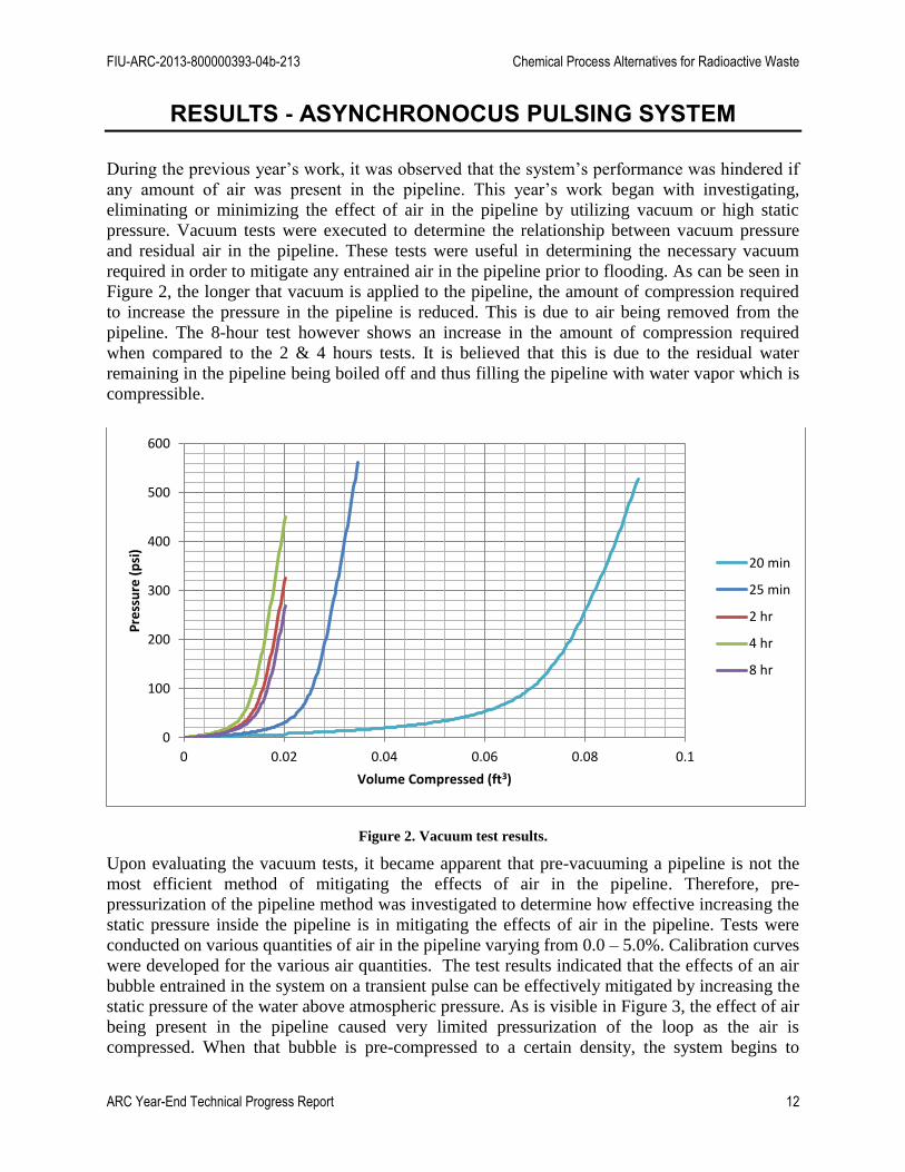
During the previous year’s work, it was observed that the system’s performance was hindered if
any amount of air was present in the pipeline. This year’s work began with investigating,
eliminating or minimizing the effect of air in the pipeline by utilizing vacuum or high static
pressure. Vacuum tests were executed to determine the relationship between vacuum pressure
and residual air in the pipeline. These tests were useful in determining the necessary vacuum
required in order to mitigate any entrained air in the pipeline prior to flooding. As can be seen in
Figure 2, the longer that vacuum is applied to the pipeline, the amount of compression required
to increase the pressure in the pipeline is reduced. This is due to air being removed from the
pipeline. The 8-hour test however shows an increase in the amount of compression required
when compared to the 2 & 4 hours tests. It is believed that this is due to the residual water
remaining in the pipeline being boiled off and thus filling the pipeline with water vapor which is
compressible.
Figure 2. Vacuum test results.
Upon evaluating the vacuum tests, it became apparent that pre-vacuuming a pipeline is not the
most efficient method of mitigating the effects of air in the pipeline. Therefore, pre-
pressurization of the pipeline method was investigated to determine how effective increasing the
static pressure inside the pipeline is in mitigating the effects of air in the pipeline. Tests were
conducted on various quantities of air in the pipeline varying from 0.0 – 5.0%. Calibration curves
were developed for the various air quantities. The test results indicated that the effects of an air
bubble entrained in the system on a transient pulse can be effectively mitigated by increasing the
static pressure of the water above atmospheric pressure. As is visible in Figure 3, the effect of air
being present in the pipeline caused very limited pressurization of the loop as the air is
compressed. When that bubble is pre-compressed to a certain density, the system begins to
0
100
200
300
400
500
600
0 0.02 0.04 0.06 0.08 0.1
Pre
ssu
re (
psi
)
Volume Compressed (ft3)
20 min
25 min
2 hr
4 hr
8 hr

FIU-ARC-2013-800000393-04b-213 Chemical Process Alternatives for Radioactive Waste
ARC Year-End Technical Progress Report 13
respond to a volume reduction in a similar manner to a no-air system. This behavior can be
exploited to ensure larger pressure changes (i.e. more force loading) at the plug face. The
observed relationship can now be used to determine the minimum static pressure required so that
the air/water mixture can act as a water-only system. The pre-pressurized value should be the
minimum at which the compressibility of the system resembles the compressibility of water.
These relationships can now be used to establish how much air can remain in longer pipe loops,
and what will be the minimum static pressure required to cause significant dynamic loading of
the plug during pulsing.
Figure 3. Calibration curves for various air quantities.
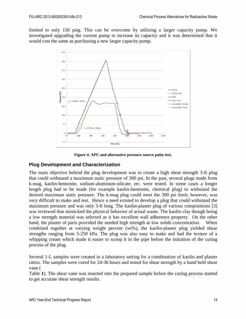
Alternate pulsing system
Research began on the development of an alternate pulsing system. Initial tests were conducted
on a small positive displacement pump arranged with two solenoid valves; one on the discharge
side of the pump and another on the suction side. By sequentially operating the valves, a positive
pressure pulse is delivered to the pipeline that is then followed by a suction phase. The benefit of
utilizing a pump as the pressure source instead of a piston is that the pump will provide more
flexibility in the volumetric flow during the pressure and suction phases. Results from the initial
tests proved to be successful and work began on configuring a large progressive cavity pump to
perform large scale testing on the pipeline. A large progressive cavity pump was plumbed to be
used as an alternative pressure source to perform asynchronous pulsing tests on the pipeline. A
side-by-side comparative test was conducted on both the alternative pressure source (large
progressive cavity pump) and the current asynchronous pulse unit. It was determined that they
behave similarly; however, as can be seen by Figure 4, the alternative pressure source was
FIU-ARC-2013-800000393-04b-213 Chemical Process Alternatives for Radioactive Waste
ARC Year-End Technical Progress Report 14
limited to only 150 psig. This can be overcome by utilizing a larger capacity pump. We
investigated upgrading the current pump to increase its capacity and it was determined that it
would cost the same as purchasing a new larger capacity pump.
Figure 4. APU and alternative pressure source pulse test.
Plug Development and Characterization
The main objective behind the plug development was to create a high shear strength 3-ft plug
that could withstand a maximum static pressure of 300 psi. In the past, several plugs made from
k-mag, kaolin-bentonite, sodium-aluminum-silicate, etc. were tested. In some cases a longer
length plug had to be made (for example kaolin-bentonite, chemical plug) to withstand the
desired maximum static pressure. The k-mag plug could meet the 300 psi limit; however, was
very difficult to make and test. Hence a need existed to develop a plug that could withstand the
maximum pressure and was only 3-ft long. The kaolin-plaster plug of various compositions [3]
was reviewed that mimicked the physical behavior of actual waste. The kaolin clay though being
a low strength material was selected as it has excellent wall adherence property. On the other
hand, the plaster of paris provided the needed high strength at low solids concentration. When
combined together at varying weight percent (wt%), the kaolin-plaster plug yielded shear
strengths ranging from 5-250 kPa. The plug was also easy to make and had the texture of a
whipping cream which made it easier to scoop it in the pipe before the initiation of the curing
process of the plug.
Several 1-L samples were created in a laboratory setting for a combination of kaolin and plaster
ratios. The samples were cured for 24-36 hours and tested for shear strength by a hand held shear
vane (
Table 1). The shear vane was inserted into the prepared sample before the curing process started
to get accurate shear strength results.

FIU-ARC-2013-800000393-04b-213 Chemical Process Alternatives for Radioactive Waste
ARC Year-End Technical Progress Report 15
Table 1. Plug Composition and Properties
No. Material Composition (wt%) Shear Strength (kPa)
1
Kaolin
Plaster
Water
50
12
38
2±0.30
2
Kaolin
Plaster
Water
30.0
27.5
42.5
28±4
3
Kaolin
Plaster
Water
40.0
22.5
37.5
135±25
4
Kaolin
Plaster
Water
35
30
35
225±25
5
Kaolin
Plaster
Water
30
35
35
>2501
It was observed that the success of making this plug was highly affected by the plug procedure
and conditions. For example the mixing time yielded different shear strengths for the same
composition. Hence, best practices relevant to the manufacturing of the plug were discussed with
an AEM consulting engineer and the recommendations were incorporated while developing the
plug.
Pressure blowout tests were conducted on a variety of 3-ft kaolin-plaster plugs made from
different recipes and with different curing times (Figure 5). The purpose of these tests was to
verify that the plugs could withstand a maximum static pressure of 300 psi. The optimal plug
was found to be 30% kaolin, 35% plaster and 35% water (by weight) with a 4-day curing time.
This combination provided a blowout pressure between 400 and 420 psi.
1 The hand held shear vane was limited to 250 kPa shear strength measurements.

FIU-ARC-2013-800000393-04b-213 Chemical Process Alternatives for Radioactive Waste
ARC Year-End Technical Progress Report 16
Figure 5. Pressure blowout tests.
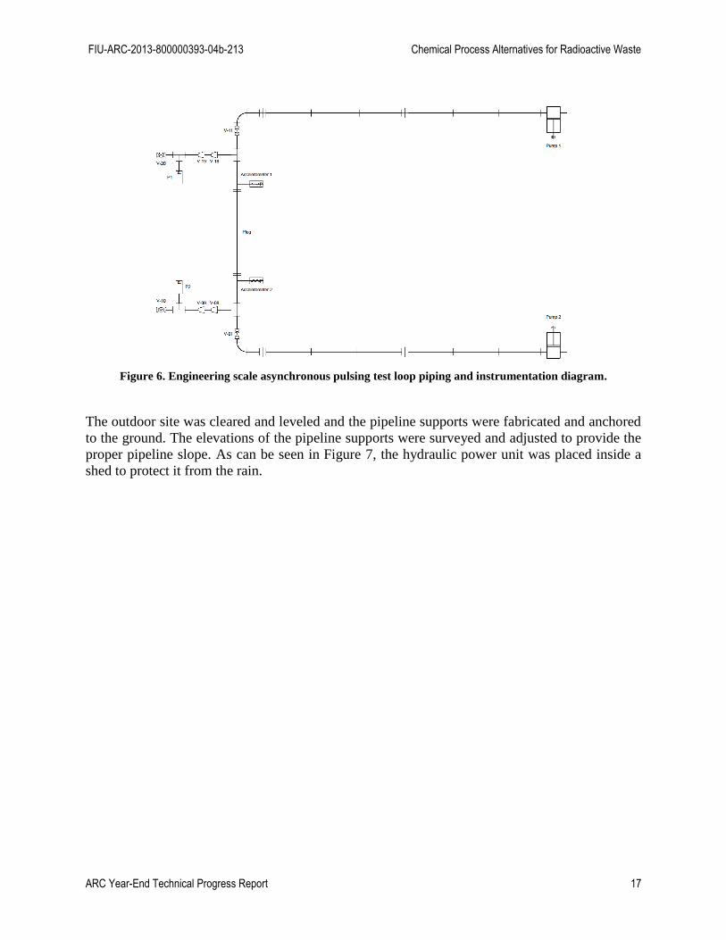
Engineering scale asynchronous pulsing unplugging trials
A test loop was designed to test the APS and its functionality on a large scale, not previously
tested. Figure 6 shows the piping and instrumentation diagram of the engineering scale loop
which consists of two 135-foot runs on either side of a plug.
FIU-ARC-2013-800000393-04b-213 Chemical Process Alternatives for Radioactive Waste
ARC Year-End Technical Progress Report 17
Figure 6. Engineering scale asynchronous pulsing test loop piping and instrumentation diagram.
The outdoor site was cleared and leveled and the pipeline supports were fabricated and anchored
to the ground. The elevations of the pipeline supports were surveyed and adjusted to provide the
proper pipeline slope. As can be seen in Figure 7, the hydraulic power unit was placed inside a
shed to protect it from the rain.

FIU-ARC-2013-800000393-04b-213 Chemical Process Alternatives for Radioactive Waste
ARC Year-End Technical Progress Report 18
Figure 7. Engineering scale testbed images for asynchronous pulsing system.
To prepare for the parametric testing of the system, data acquisition software changes were
made. During the initial testing, some hardware problems were encountered concurrent with
placing the system in an outdoor wet environment. Even though the new pressure transducers
were verified to be working properly after installation, during initial system tests several
transducers failed. It is believed that water intrusion is the issue since it had rained in the days
leading up to the failures. Furthermore, since the transducer connectors had been previously
used, they did not form a very tight seal around the transducer terminals; therefore, each
connector was filled with non-dielectric silicone.
Additional issues related to the pump’s linear position transducers were also observed. Both
linear position transducers failed, with the cause believed to be water damage. Both linear
transducers were sent to the manufacturer for assessment and repair. It was determined that the
damage was due to either “an external overvoltage [or] stray power applied to the ground”.
During our failure analysis, the step-down transformer was also found to be damaged. It had
failed, delivering only half of the designed voltage. The transformer was also equipped with a
voltage rectifier, thus, eliminating the overvoltage scenario as a possible cause. Corrective

FIU-ARC-2013-800000393-04b-213 Chemical Process Alternatives for Radioactive Waste
ARC Year-End Technical Progress Report 19
actions were taken to eliminate the step-down transformer from the control/data acquisition
system circuit. In addition, the control/data acquisition system was directly connected to a
grounded power supply with a surge protector. To eliminate any future water infiltration, new
gaskets and connectors for the pressure transducers were also purchased and miniature
enclosures were constructed for each location where the transducers are exposed to the elements.
After the pumps’ repaired linear position transducers were received, they were installed and the
wiring was tested. Upon testing of the electrical wiring for the linear position transducers, a stray
power-to-ground was discovered and repaired. This coincides with the findings of the
manufacturer of the linear position transducers. Once repaired, the transducers were wired and
found to be operating correctly.
Once all the electrical issues were addressed, test finally began on the engineering scale loop.
Initial tests were a single pressure pulse tests that were intended to determine the pressure pulse
amplification within the pipeline. Tests were conducted at both 0 and 50 psi static pressures.
Figure 8. Single pressure pulse results with a 0 psi static pressure.
FIU-ARC-2013-800000393-04b-213 Chemical Process Alternatives for Radioactive Waste
ARC Year-End Technical Progress Report 20
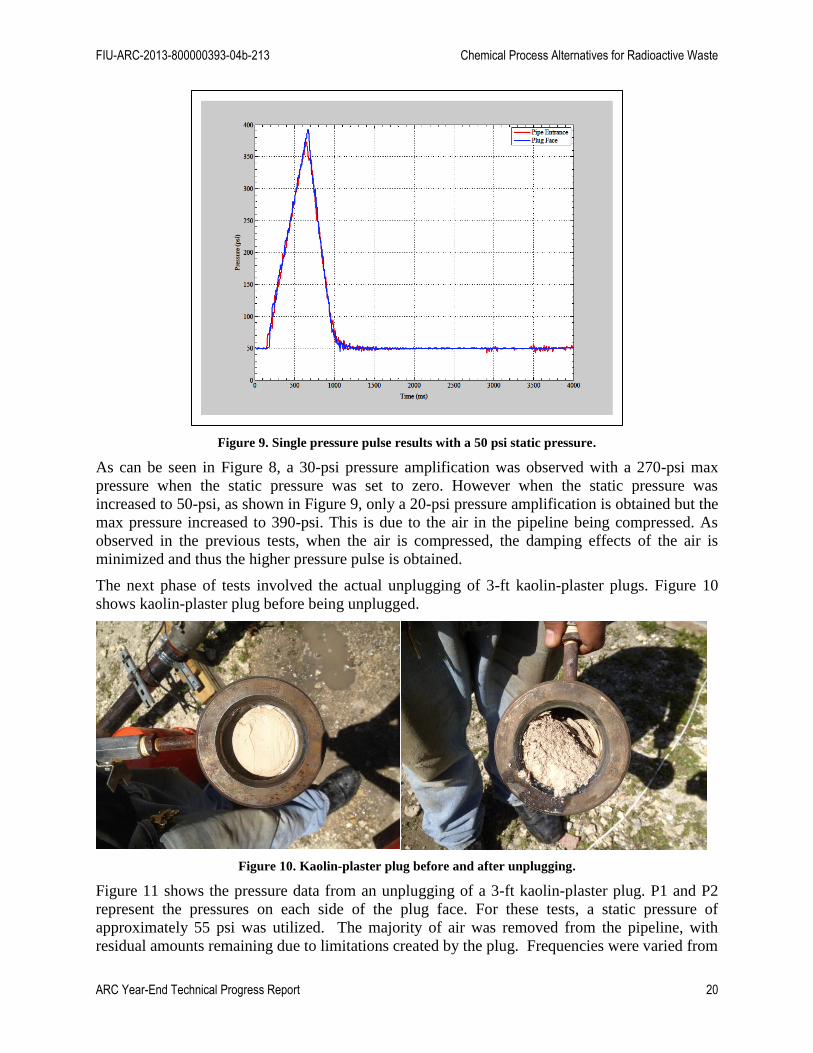
Figure 9. Single pressure pulse results with a 50 psi static pressure.
As can be seen in Figure 8, a 30-psi pressure amplification was observed with a 270-psi max
pressure when the static pressure was set to zero. However when the static pressure was
increased to 50-psi, as shown in Figure 9, only a 20-psi pressure amplification is obtained but the
max pressure increased to 390-psi. This is due to the air in the pipeline being compressed. As
observed in the previous tests, when the air is compressed, the damping effects of the air is
minimized and thus the higher pressure pulse is obtained.
The next phase of tests involved the actual unplugging of 3-ft kaolin-plaster plugs. Figure 10
shows kaolin-plaster plug before being unplugged.
Figure 10. Kaolin-plaster plug before and after unplugging.
Figure 11 shows the pressure data from an unplugging of a 3-ft kaolin-plaster plug. P1 and P2
represent the pressures on each side of the plug face. For these tests, a static pressure of
approximately 55 psi was utilized. The majority of air was removed from the pipeline, with
residual amounts remaining due to limitations created by the plug. Frequencies were varied from

FIU-ARC-2013-800000393-04b-213 Chemical Process Alternatives for Radioactive Waste
ARC Year-End Technical Progress Report 21
0.5 to 2 Hz, however, transducer issues arose at 2 Hz. Resulting pulse amplitudes were
dependent on valve opening, frequency/piston speed and air entrainment. After analyzing the
data it was observed that P2 had a smaller pressure range than P1 for the 1.5 Hz trial. This is
believed to be due to the P2 side of the pipe loop containing more air than the P1 side. Another
observation was that just before unplugging occurred P1 started to increase as P2 was
decreasing. This is due to water starting to leak past the plug from the P2 side to the P1 side. The
decrease in the water volume from one side will cause the pressure per stroke to decrease while
the increase of water volume on the other side will cause the pressure per stroke to increase.
Figure 11. Pressure data from an unplugging of a kaolin-plaster plug at 1.5 Hz.
Figure 12 shows the pressures for a 0.5 Hz trial. As with the previous test, P2 had a larger
pressure range than P1. This is also believed to be due to air still remaining in the P1 side of the
loop. Also in this test, water started to leak past the plug from the P1 side to the P2 side which
resulted in P2 starting to increase as P1 was decreasing just before unplugging occurred.

FIU-ARC-2013-800000393-04b-213 Chemical Process Alternatives for Radioactive Waste
ARC Year-End Technical Progress Report 22
Figure 12. Pressure data from an unplugging of a kaolin-plaster plug at 0.5 Hz.
Figure 13 shows the data from the accelerometers mounted on the pipeline on both sides of the
plug for the 0.5 Hz trial. As can be seen from the graph, the force applied to the pipeline started
to increase as just before the plug was unplugged and reached its maximum when unplugging
occurred.
Figure 13. Pipeline accelerometer data during a 0.5 Hz unplugging.
FIU-ARC-2013-800000393-04b-213 Chemical Process Alternatives for Radioactive Waste
ARC Year-End Technical Progress Report 23
Discussion
After analyzing the data of the APS on a large scale loop, several observations were made. As in
the previous testing done on smaller loops, air in the system has a major effect on the system’s
performance. Just as in the tests conducted on smaller loops, the consequence of entrained air
can be mitigated by either applying a vacuum to the pipeline or increasing the system’s static
pressure. The data obtained from this testing indicates that increasing the static pressure is a
more effective method. During previous testing, the pulsing frequency played a major role in the
system’s unplugging capability. However, during these tests on the larger loop this was not
observed which is believed to be due to the longer pipeline length damping the frequency.

FIU-ARC-2013-800000393-04b-213 Chemical Process Alternatives for Radioactive Waste
ARC Year-End Technical Progress Report 24
ENGINEERING SCALE PIPELINE UNPLUGGING TESTING USING THE PERSITALTIC CRAWLER SYSTEM
Background
FIU’s efforts to develop innovative pipeline unplugging technologies include the development of
a crawler system that can conduct unplugging operations. The PCS is a pneumatic/hydraulic unit
that can navigate inside a pipeline by pressurization/depressurization of flexible cavities. To date,
three generations of the PCS have been designed, assembled, and tested each one having
improvements to overcome the limitations previously observed. For each generation, the tests
conducted on bench-scale testbed have provided information on the navigational speed, ability to
negotiate thru a 90° elbow, pull force, and unplugging ability. Design improvements to bolster its
durability and have also been implemented on each generation.
The current system consists of a crawler unit, a tether-reel assembly and a control station. The
unplugging tool is attached to the front of the unit and powered by pressurized water. The
crawler unit has a double walled bellow assembly and a front and back rim to which flexible
sleeves are clamped forming the front and back cavities. The center of the double walled bellow
assembly creates a passage that allow particles of the plug that are set loose during the
unplugging process to travel to the back of the unit. Attached to the front rim is a nose cap
designed to hold the unplugging tools (high pressure water nozzle) and the camera. Figure 14(a)
shows a rendering of the crawler unit and (b) shows an exploded view of the crawler assembly.
(a) (b)
Figure 14. (a) Rendering of crawler, (b) exploded view of crawler assembly [4].
The tether connects the crawler to the control station and the power supply source. The tether
consists of three pneumatic lines, one hydraulic line, and one multi-conductor cable jacketed
together having a total length of 500 ft. The reel system was designed to accommodate the tether
and provides rotating connections to the pneumatic, hydraulic, and electrical lines (Figure 15
(a)). The control station includes the pneumatic pressure regulators, a vacuum pump, vacuum
chamber and a controller box containing a programmable logic controller (PLC) that controls the
position (opened/closed) pneumatic valves of the crawler unit. By programming an appropriate
sequence on the PLC, the desired motion is achieved (Figure 15 (b)).

FIU-ARC-2013-800000393-04b-213 Chemical Process Alternatives for Radioactive Waste
ARC Year-End Technical Progress Report 25
(a) (b)
Figure 15. (a) Reel system, (b) control station.
Design Improvements
For this performance period, efforts focus on meeting the necessary requirements that will enable
the PCS to conduct unplugging and inspection operations in a 430-ft pipeline. Improvements to
the system include the re-design of the rims of the unit to accommodate a camera system to
provide visual feedback of the conditions inside the pipeline, positioning of a pneumatic valve
manifold system located in close proximity to the crawler and optimization of the double bellow
assembly to reduce cycle time.
The tether was connected and wound to the reel system. The reel has rotating
manifold/connectors for pneumatic, hydraulic and electrical lines. The rotating manifold consists
of four 1/4”FNPT ports and 6 electrical conductors. The reel makes controlling the length of
tether routed thru the inlet point easy to control and prevents the pneumatic and hydraulic lines
from damage due to kinking. Figure 16 (a) shows the tether attached to the crawler, and Figure
16 (b) shows the tether wound to the reel system.
Figure 16. (a)Tether attached to the crawler, (b) tether-reel assembly.

FIU-ARC-2013-800000393-04b-213 Chemical Process Alternatives for Radioactive Waste
ARC Year-End Technical Progress Report 26
Previous tests conducted using different tether lengths demonstrated that there is a significant
reduction in speed of the crawler with increasing length of the tether. This decrease in speed is
the result of the increase of volume required to be pressurized/depressurized inside the tether
before the set pressure can be reached at the cavity in the crawler unit for each cycle. In previous
tests, a speed of 1 ft/hr was recorded using a 500-foot tether which shows that in order for the
PCS to be effective in longer pipelines, it would require design changes to reduce the cycle time.
A solution to eliminate pressurizing/depressurizing the tether with each cycle was implemented
by relocating the pneumatic valves from the control to a trailing capsule located approximately 1
ft from the rear of the unit. This change allows the pneumatic lines of the tether assembly to
remain at a constant pressure, making the cycle time independent of tether length. The capsule
encases 3 12-volt pneumatic valves connected to the tether assembly. The valves used are single
acting Bullet Valves manufacture by MAC Valves, Inc. Each of the valves is connected to the
PLC using the electrical lines of the tether and each controls a separate cavity of the crawler.
Figure 17 (a) shows a rendering of the design of the capsule and valves and Figure 17 (b) shows
the assembled capsule manufactured using ABS (acrylonitrile butadiene styrene).
(a) (b)
Figure 17. (a) Rendering of capsule, (b) capsule manufactured from ABS.
As noted in the introduction, an improvement to the crawler was the implementation of a visual
feedback system that provides images of the conditions inside the pipeline. Several commercially
available systems were evaluated based on their compatibility with the crawler requirements.
The criteria for selection included that the visual feedback system should not hamper the
navigational capabilities of the unit, must be small enough to be contained within the crawler,
must be able to operate at a minimum distance of 1000 ft from the inlet point and must be able to
operate in a HLW environment. The visual system selected was the INUKTUN Mini-Cristal
Cam®. This system uses a camera that is 7/8” in diameter and connects to a display station
using a fiber optic cable. It has an operational range of 1000 ft and can function in HLW
environments up to 300 rad/hour. Additionally, the system is provided with a light source to
illuminate dark environments. Figure 18 shows a close-up of the camera and the display station.
FIU-ARC-2013-800000393-04b-213 Chemical Process Alternatives for Radioactive Waste
ARC Year-End Technical Progress Report 27
Figure 18. (a) Camera, (b) display station.
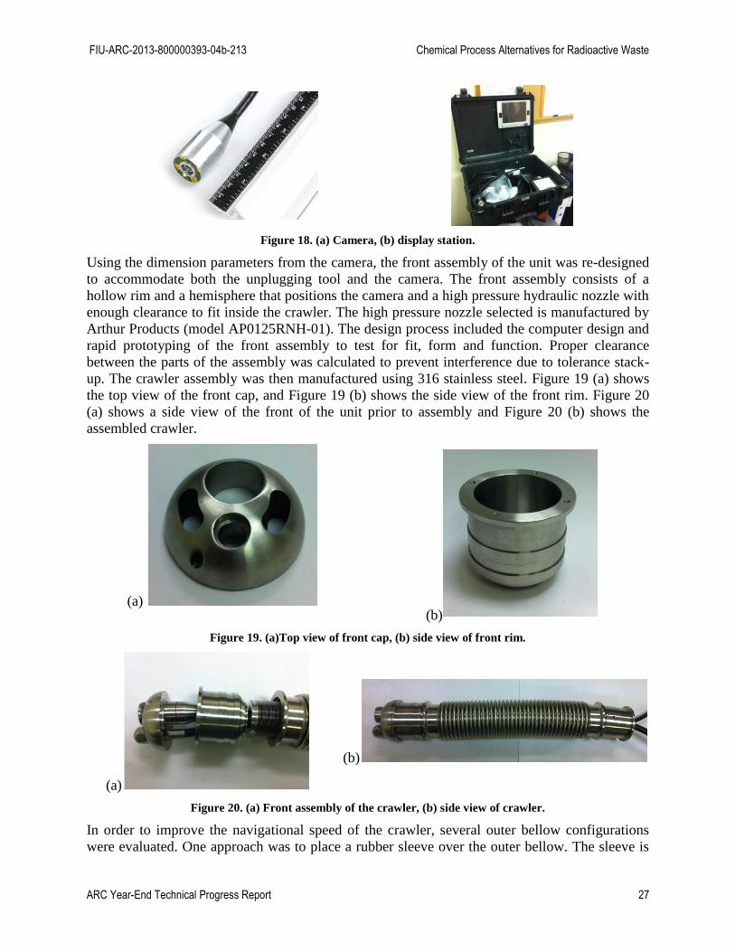
Using the dimension parameters from the camera, the front assembly of the unit was re-designed
to accommodate both the unplugging tool and the camera. The front assembly consists of a
hollow rim and a hemisphere that positions the camera and a high pressure hydraulic nozzle with
enough clearance to fit inside the crawler. The high pressure nozzle selected is manufactured by
Arthur Products (model AP0125RNH-01). The design process included the computer design and
rapid prototyping of the front assembly to test for fit, form and function. Proper clearance
between the parts of the assembly was calculated to prevent interference due to tolerance stack-
up. The crawler assembly was then manufactured using 316 stainless steel. Figure 19 (a) shows
the top view of the front cap, and Figure 19 (b) shows the side view of the front rim. Figure 20
(a) shows a side view of the front of the unit prior to assembly and Figure 20 (b) shows the
assembled crawler.
(a) (b)
Figure 19. (a)Top view of front cap, (b) side view of front rim.
(a)
(b)
Figure 20. (a) Front assembly of the crawler, (b) side view of crawler.
In order to improve the navigational speed of the crawler, several outer bellow configurations
were evaluated. One approach was to place a rubber sleeve over the outer bellow. The sleeve is

FIU-ARC-2013-800000393-04b-213 Chemical Process Alternatives for Radioactive Waste
ARC Year-End Technical Progress Report 28
placed over the compressed bellow during assembly. This configuration provides a faster
compression time of the bellow. Three sleeve thicknesses were evaluated 0.004, 0.0625, and
0.125 inches. Figure 21 shows the crawler with a 0.125 in thick sleeve. An additional
configuration was to replace the outer hydroformed bellow with one having similar overall
dimension but smaller thickness. A thinner wall bellow reduces the force required for the crawler
to reach full compression.
Figure 21. Crawler with a 0.125 in thick sleeve.
Testbeds
The experimental testing of the PCS was conducted using a bench scale testbed and an
engineering scale testbed. Similar to the testbed used previously, the bench scale tested consisted
of two 3-ft long clear PVC straight sections connected with a 90° elbow and a 3-ft long carbon
steel section. All of the pipes are 3 inches in diameter. Figure 22 shows the testbed used to
conduct the navigation tests.
Figure 22. Bench scale testbed.
To experimentally determine the pull force that the crawler unit can generate, the crawler was
placed inside a fixture consisting of a clear pipe section containing a spring of known stiffness
(Figure 23). The testing procedure consisted on first pressurizing the back cavity to anchor the
unit to the pipeline to then provide different pressure to the double wall assembly. The
displacement of the front end of the crawler unit was recorded to calculate the force generated.
FIU-ARC-2013-800000393-04b-213 Chemical Process Alternatives for Radioactive Waste
ARC Year-End Technical Progress Report 29
Figure 23. Fixture used to determine the crawler unit force.
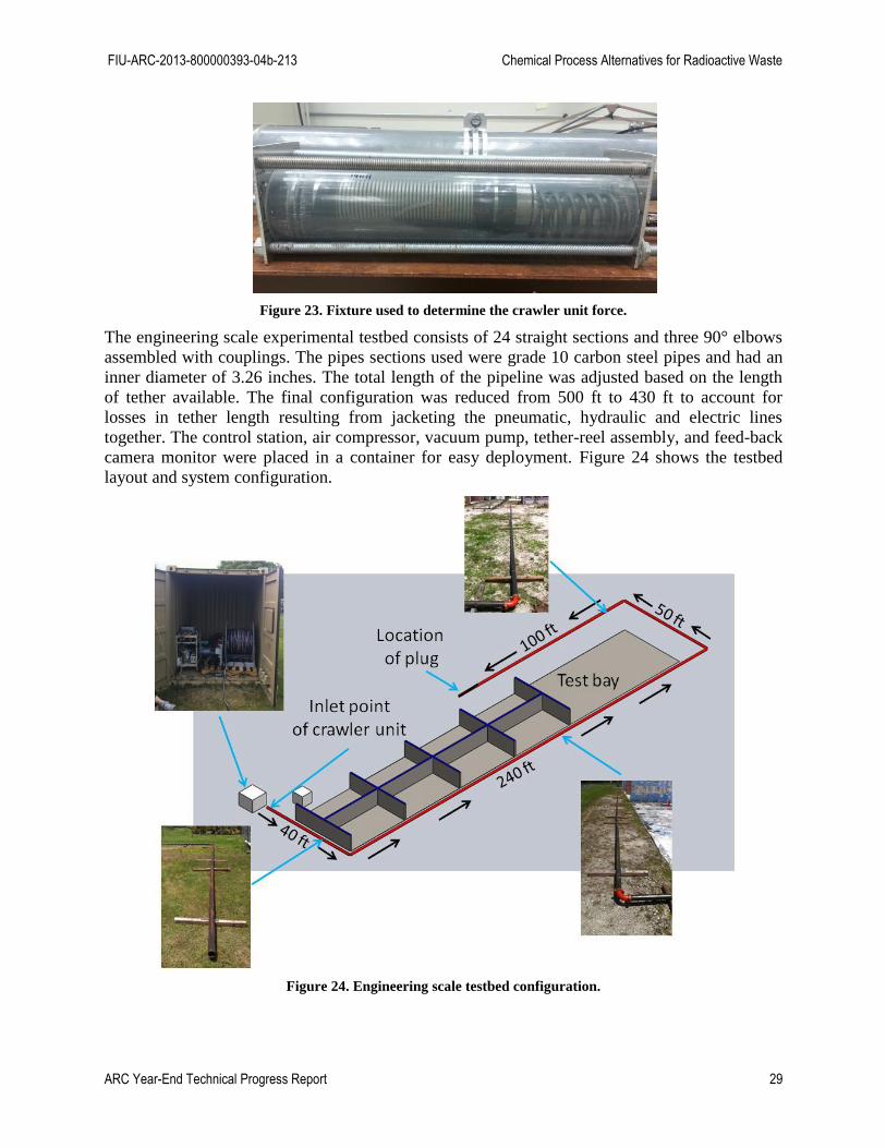
The engineering scale experimental testbed consists of 24 straight sections and three 90° elbows
assembled with couplings. The pipes sections used were grade 10 carbon steel pipes and had an
inner diameter of 3.26 inches. The total length of the pipeline was adjusted based on the length
of tether available. The final configuration was reduced from 500 ft to 430 ft to account for
losses in tether length resulting from jacketing the pneumatic, hydraulic and electric lines
together. The control station, air compressor, vacuum pump, tether-reel assembly, and feed-back
camera monitor were placed in a container for easy deployment. Figure 24 shows the testbed
layout and system configuration.
Figure 24. Engineering scale testbed configuration.
FIU-ARC-2013-800000393-04b-213 Chemical Process Alternatives for Radioactive Waste
ARC Year-End Technical Progress Report 30
RESULTS
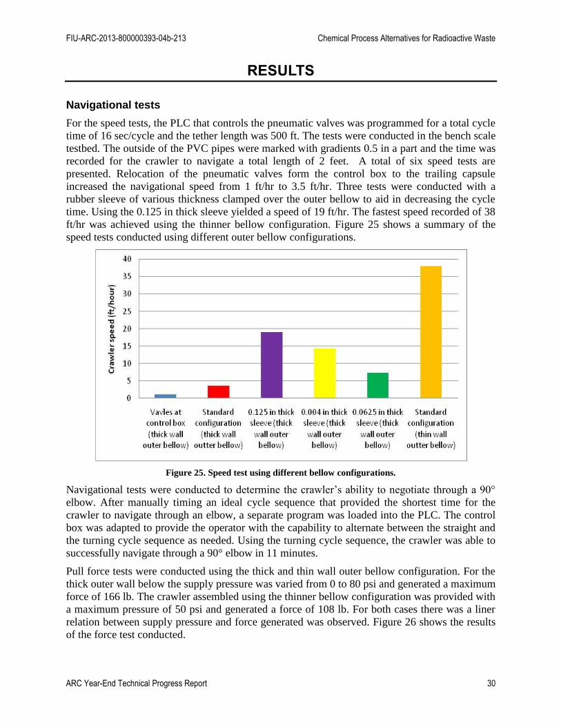
Navigational tests
For the speed tests, the PLC that controls the pneumatic valves was programmed for a total cycle
time of 16 sec/cycle and the tether length was 500 ft. The tests were conducted in the bench scale
testbed. The outside of the PVC pipes were marked with gradients 0.5 in a part and the time was
recorded for the crawler to navigate a total length of 2 feet. A total of six speed tests are
presented. Relocation of the pneumatic valves form the control box to the trailing capsule
increased the navigational speed from 1 ft/hr to 3.5 ft/hr. Three tests were conducted with a
rubber sleeve of various thickness clamped over the outer bellow to aid in decreasing the cycle
time. Using the 0.125 in thick sleeve yielded a speed of 19 ft/hr. The fastest speed recorded of 38
ft/hr was achieved using the thinner bellow configuration. Figure 25 shows a summary of the
speed tests conducted using different outer bellow configurations.
Figure 25. Speed test using different bellow configurations.
Navigational tests were conducted to determine the crawler’s ability to negotiate through a 90°
elbow. After manually timing an ideal cycle sequence that provided the shortest time for the
crawler to navigate through an elbow, a separate program was loaded into the PLC. The control
box was adapted to provide the operator with the capability to alternate between the straight and
the turning cycle sequence as needed. Using the turning cycle sequence, the crawler was able to
successfully navigate through a 90° elbow in 11 minutes.
Pull force tests were conducted using the thick and thin wall outer bellow configuration. For the
thick outer wall below the supply pressure was varied from 0 to 80 psi and generated a maximum
force of 166 lb. The crawler assembled using the thinner bellow configuration was provided with
a maximum pressure of 50 psi and generated a force of 108 lb. For both cases there was a liner
relation between supply pressure and force generated was observed. Figure 26 shows the results
of the force test conducted.
FIU-ARC-2013-800000393-04b-213 Chemical Process Alternatives for Radioactive Waste
ARC Year-End Technical Progress Report 31
Figure 26. Force tests results.
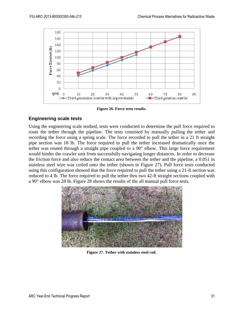
Engineering scale tests
Using the engineering scale testbed, tests were conducted to determine the pull force required to
route the tether through the pipeline. The tests consisted by manually pulling the tether and
recording the force using a spring scale. The force recorded to pull the tether in a 21 ft straight
pipe section was 18 lb. The force required to pull the tether increased dramatically once the
tether was routed through a straight pipe coupled to a 90° elbow. This large force requirement
would hinder the crawler unit from successfully navigating longer distances. In order to decrease
the friction force and also reduce the contact area between the tether and the pipeline, a 0.051 in
stainless steel wire was coiled onto the tether (shown in Figure 27). Pull force tests conducted
using this configuration showed that the force required to pull the tether using a 21-ft section was
reduced to 4 lb. The force required to pull the tether thru two 42-ft straight sections coupled with
a 90° elbow was 28 lb. Figure 28 shows the results of the all manual pull force tests.
Figure 27. Tether with stainless steel coil.

FIU-ARC-2013-800000393-04b-213 Chemical Process Alternatives for Radioactive Waste
ARC Year-End Technical Progress Report 32
Figure 28. Manual tether pulling force for different pipeline lengths.
Rims fatigue tests
Previous bench scale navigational tests were conducted using PVC pipe sections. The inner
diameter of the PVC pipes was 2.9 inches. The carbon steel schedule 10 pipes used in the
engineer scale testbed have an inner diameter of 3.26 inches. The increase in the distance
between the crawler and the pipeline wall requires the front and back cavities to expand further
in order to anchor the crawler unit to the pipeline. During the navigational tests, this additional
expansion caused the cavities to rupture after the crawler reached approximately 10 feet from the
inlet point of the pipeline. Based on the projected displacement of the crawler per cycle, it is
estimated that total of 3,600 cycles would be required for the unit to navigate a 500-ft pipeline.
For all tests, the rupture occurred at the stress risers created at the clamps edges. In an attempt to
eliminate the failure of the cavities, different materials, configurations, and clamping pressures
were tested. The largest number of cycles recorded without failure was 1,260 using a Kevlar
gasket placed between the clamps and the flexible cavity. Figure 29 (a) shows the crawler unit’s
back rim using a 0.125 in thick material and Figure 29 (b) show a failure due to insufficient
clamping force.
(a) (b)
Figure 29. (a)Back rim with 0.125 in thick flexible gum, (b)failure due to insufficient clamping force.

FIU-ARC-2013-800000393-04b-213 Chemical Process Alternatives for Radioactive Waste
ARC Year-End Technical Progress Report 33
An alternative approach to reach the 3,600 cycles without failure is to increase the distance
between the clamps. This increment provides additional available material that can expand to
reach the inner pipeline wall. An experimental fixture having the same outer diameter as the back
rim was assembled and test were performed in a schedule 10 pipeline section. Two tests were
performed: one having a distance between clamps of 1.75 in and the other a distance of 1 inch.
The test for the 1.75 in provided a total of over 14,000 cycles with no evidence of failure. The
test for the 1 inch clamp distance held for a total of over 15,000 cycles prior to failure. Figure 30
(a) shows the experimental fixture and Figure 30 (b) shows the test conducted using the 1 inch
clamp distance.
(a) (b)
Figure 30. Experimental fixture and experimental fixture inside pipeline section.
Using the experimental result from the fixture, prototypes of the rims having an additional length
of 0.5 in to provide 1.25 in of distance between clamps were prototyped and the crawler was then
assembled. A pull test in a 90° elbow was conducted by routing a wire through the crawler and
attaching it to the rear rim. Tests showed that the increased length of the rims caused the crawler
to wedge against the inner surfaces of the elbow preventing it from turning. A second set of rims
having 0.25 in of additional length (1 in of distance between clamps) were prototyped and tested
using the same procedure. With these rims, the crawler was able to successfully navigate through
a 90° elbow with a pull force of 12 lb. Figure 31(a) show the crawler unit with prototype rims
and Figure 31(b) shows the crawler unit assembled with a clamp distance of 1.25 inches.
(a)
(b)
Figure 31. Crawler unit with prototype rims, assemble front end of crawler unit.

FIU-ARC-2013-800000393-04b-213 Chemical Process Alternatives for Radioactive Waste
ARC Year-End Technical Progress Report 34
CONCLUSIONS AND FUTURE WORK
Two technologies, APS and a peristaltic crawler, have continued to be developed and evaluated
during FIU Year 3.
The APS was used on an engineering scale testbed consisting of a symmetric configuration using
approximately 135-ft of 3-inch sch-40 threaded pipe with one 90° elbow on each side of a plug.
A 3-ft the kaolin-plaster plug was placed in the middle of the testbed and different pulse
frequencies were applied to plug. After analyzing the data, several observations were made. As
in the previous testing done on smaller loops, air in the system has a major effect on the system’s
performance. Just as in the tests conducted on smaller loops, the consequence of entrained air
can be mitigated by either applying a vacuum to the pipeline or increasing the system’s static
pressure. The data obtained from this testing indicates that increasing the static pressure is a
more effective method. During previous testing, the pulsing frequency played a major role in the
system’s unplugging capability. However, during these tests on the larger loop this was not
observed which is believed to be due to the longer pipeline length damping the frequency.
During this phase of testing, several electronic failures were encountered, including pressure
transducers and linear position transducers. This is believed to be due to locating the system
outside in the elements. Future work will begin with a full analysis of the failures and
determining what changes to the system design need to be done to prevent such failures from
happening in the future. In addition, due to the size of the pipeline purging the all the air from the
pipes was difficult. This too will be investigated to develop a better air purging method.
The tests conducted showed that the improvements in the design of the PCS have a significant
effect on its navigational performance using the bench scale testbed. The relocation of the valves
from the control box to the trailing capsule increased the speed of the crawler by 350%. An
additional improvement in speed was observed using the thinner wall outer bellow which
provided a speed of 38 ft/hr. The addition of the sleeve using the thicker wall outer bellow
showed a maximum speed of 19 ft/hr. However, the use of a sleeve has the potential of
hampering the crawler’s maneuverability through a 90° elbow since it increases the radial
stiffness of the crawler as well as creates a higher friction surface with the inner pipeline.
The force tests conducted showed that the thick wall and thin wall bellow have a similar
response to force generated due to the supplied air pressure. The tests using the thin wall bellow
was not taken above 50 psi to prevent potential permanent deformation. Future tests will include
pressurizing the thin wall bellow to failure and fatigue tests to determine the acceptable life limit
of the bellow. The use of the 0.051 in stainless steel wire wounded around the tether significantly
reduced the pull force required to route the tether through the pipeline. It was observed that an
increment of 8 lb was required per every 21-ft section of straight pipe. Routing the tether
through an elbow required an increase of 33% in the force. Future test will include routing the
tether and measuring the pull force through the remaining three elbows of the engineering scale
testbed.
The difference in inner pipe wall diameter between the PVC pipe sections and schedule 10 pipe
sections (2.9 in and 3.26 in, respectively) had a significant effect on the life of the rim cavities.
Tests showed that a distance between clamps of at least 1 in is required to provide 14,000 cycles
with no failure. The use of gaskets to decrease the stress rises at the clamps locations was not
sufficient to prevent failure above acceptable limits (3,600 cycles). The prototype having a 0.25

FIU-ARC-2013-800000393-04b-213 Chemical Process Alternatives for Radioactive Waste
ARC Year-End Technical Progress Report 35
in longer rims provided a clamps distance of 1 in and does not increase the force required for the
crawler to navigate through an elbow. Future efforts will include manufacturing a stainless steel
crawler with the dimensions of the prototype.
During the next period, final adjustments to the PCS will be implemented and the system will be
tested using the total length of the engineering testbed (430 ft). Future tests will include
performing unplugging and inspection operations.

FIU-ARC-2013-800000393-04b-213 Chemical Process Alternatives for Radioactive Waste
ARC Year-End Technical Progress Report 36
REFERENCES
1. Roelant, D., (2012). FY2011 Year End Technical Report. Chemical Process Alternatives for
Radioactive Waste. U.S. Department of Energy, Office of Environmental Management.
2. Zollinger, W., & Carney, F. (2004). Pipeline blockage unplugging and locating equipment.
Conference on Robotics and Remote Systems- Proceedings, (pp. 80 - 85). Gainesville.
3. Golcar et al., 2000. Hanford Tank Waste Simulants Specification and Their Applicability for
the Retrieval, Pretreatment, and Vitrification Processes, Battelle, Richland, Washington.
4. Pribanic, T., Awwad, A., Varona, J., McDaniel, D., Gokaltun, S., Crespo, J. (2013). Design
Optimization of Innovative High-Level Waste Pipeline Unplugging Technologies. In
Proceedings of Waste Management Symposia, Phoenix AZ.

FIU-ARC-2013-800000393-04b-213 Chemical Process Alternatives for Radioactive Waste
ARC Year-End Technical Progress Report 37
TASK 12: MULTIPLE-RELAXATION-TIME LATTICE BOLTZMANN MODEL FOR MULTIPHASE FLOWS
EXECUTIVE SUMMARY
Many engineering processes at various U.S. Department of Energy sites include the fluid flow of
more than one phase such as air and water. Slurry mixing methods such as pulsed-air mixers, air
sparging, and pulsed-jet mixing are a few examples where more than one fluid phase can exist in
contact with another phase. Lattice Boltzmann method (LBM) is a computational fluid dynamics
(CFD) method that can provide insight into the behavior of multiphase flows by capturing the
interface dynamics accurately during the process and the effects of structures on multiple fluid
phases.
Florida International University (FIU) aims to develop LBM-based computer codes that can be
used by the U.S. DOE scientists and engineers as a prediction tool for understanding the physics
of fluid flow in nuclear waste tanks during regular operations and retrieval tasks. In FY2009, a
new task was initiated within FIU’s research project on high-level-waste (HLW) in order to
develop a computational code, which is based on the LBM in order to simulate multiphase flow
problems related to HLW operations. A thorough literature review was conducted to identify the
most suitable multiphase fluid modeling technique in LBM and a single-phase multi-relaxation-
time (MRT) code was developed. In FY2010, FIU identified and evaluated a multiphase LBM
using a single-relaxation-time (SRT) collision operator and updated the collision process in the
computer code with an MRT collision model. In FY2011, the MRT LBM code was extended
into three dimensions and the serial computer code was converted into a parallel code.
LBM requires attention when the fluid interface between multiple phases comes in contact with
solid surfaces in order to yield the correct molecular forcing exerted on the fluids by the surface.
During the current performance period, a proper contact angle model is presented within the
LBM framework that allows changing the wetting characteristics of droplets and bubbles on
solid surfaces. A procedure to incorporate complex geometries into the LBM simulation is also
presented. In addition, a literature review was conducted in order to investigate the applicability
of LBM for the simulation of non-Newtonian fluids as it is applicable to the waste mixing using
pulse-jet mixers in WTP tanks since the slurry found at Hanford is categorized as Bingham
plastic and this feature should be incorporated in the engineering calculations for accurate
estimations of the performance of various waste removal and handling operations. Various
turbulence models such as the Large Eddy Simulation model were also investigated for the
current multiphase LBM code developed at FIU. Most of the engineering problems involving
fluid flow in the DOE operations at Hanford, such as the pulse-jet mixing, involve high fluid
velocities that include turbulent effects that need to be taken into consideration in any computer
model that would be used to understand the behavior of such systems.

FIU-ARC-2013-800000393-04b-213 Chemical Process Alternatives for Radioactive Waste
ARC Year-End Technical Progress Report 38
INTRODUCTION
The storage and mixing of the liquid waste requires understanding the behavior of the fluid flow
inside the waste tanks. Multiple phases of fluids can exist inside the waste tanks where bubble
dynamics can play an important role. Gas bubbles can exist in the waste entrapped in the liquid
phase, inside cracks within the solid waste or on the surface of the tank walls. They can also be
generated inside the waste naturally caused by chemical reactions such as hydrogen production
or can be externally supplied via mechanical mechanisms such as air-purging, pulsed-air mixing
etc.
An understanding of the physical nature of bubble dynamics inside the waste and the effects of
the air release process to the tank environment need to be gained by considering various waste
conditions. Such an analysis can be made possible by developing a numerical method that can
simulate the process of air bubble generation inside tanks and that can accurately track the
interactions of the gas phase with the surrounding fluid and solid phases. The final computational
program would serve as a tool for Site engineers and scientists to predict waste behavior and
improve operational procedures during the storage, handling and transfer of liquid waste.
In this report, a numerical method based on LBM is presented, which can model multiphase
flows accurately and efficiently. LBM is advantageous over traditional Navier-Stokes based
computational models since surface forces are handled more easily in LBM. Another capability
of LBM is the straightforward integration of complex geometries which eliminates the necessity
to generate a complicated computational mesh which usually takes more time than the execution
of the simulations in classical CFD. The performance of MRT LBM for multiphase flow
simulations in complex three dimensional geometries is presented in this report.
The outline of the report is given as follows: first, the literature review conducted for modeling
turbulent flows and non-Newtonian fluid flows using LBM is covered. Then, three-dimensional
LBM method is introduced for the simulation of multiphase flows in complex geometries. The
results obtained follow and finally, conclusions are drawn and discussions for future work are
presented.
Turbulence modeling with LBM
The categorization of viscous flows falls into two types based on the structure of the flow; either
laminar flow, which is the case where the slow structure is made of a smooth variation of layers,
or turbulent flows where the flow has a random and chaotic structure [1]. The random behavior
of turbulent flows presents itself in the occurrence of swirling regions of flow, called eddies,
which can be vary in size over a wide range. Kolmogorov predicts the size of the smallest eddies
as proportional to the Reynolds number, [2]. Turbulent flow simulations are conducted
using a fine grid that resolves all aspects of the flow including the smallest eddies are called
direct numerical simulation (DNS). DNS is considered to be the most accurate numerical
simulation tool; however, the computational load for such simulations becomes tremendous for
problems that are characterized with large Reynolds numbers. In the case of a three-dimensional
model of a turbulent pulsed-jet flow in a waste tank, the jet Reynolds number can be of the order
of 104 [3] which requires the grid points to be in the order of 10
9 [4].
As a remedy, the mean values of the macroscopic values of the flow properties are calculated in
computational fluid dynamics (CFD) simulations of turbulent flows with the addition of a

FIU-ARC-2013-800000393-04b-213 Chemical Process Alternatives for Radioactive Waste
ARC Year-End Technical Progress Report 39
subgrid model for small scale details that cannot be captured with the coarse grid. The turbulence
models are needed to provide an expression for the Reynolds stress tensor that appears in the
Navier-Stokes equations as a result of the averaging process, which is also referred as the
“filtering”. Large eddy simulations use this approach to calculate an effective viscosity to predict
the effect of small eddies using coarse grid values. One popular approach is provided by
Smagorinsky [5], where the Reynolds stress tensor is calculated using the local strain rate
without the requirement of solving a separated partial differential equation.
An additional approach is to use the Reynolds Averaged Navier-Stokes (RANS) equations in
conjunction with a turbulence model such as the k-ε model to model the turbulent scales. The
Reynolds stress is represented in the k-ε model in terms of the strain rate, the turbulent kinetic
energy k and the dissipation rate ε. The addition of the two unknown variables, k and ε, requires
the solution of two additional transport equations. This approach yields time-averaged velocities
and is found to be less accurate then the LES; however, fine mesh requirement of LES requires
more computer power compared to RANS-based turbulence modeling. In summary, LES can be
considered as a compromise between DNS and RANS in terms of computational resource
requirements and accuracy.
The above discussion for various approaches to model turbulence using the Navier-Stokes
equation is also applicable to the lattice Boltzmann equation. Martinez et al. compared LBM
against pseudospectral method for decaying turbulence of a shear layer for an initial Reynolds
number of 10,000 [6]. Other two-dimensional applications include isotropic forced turbulence [7;
8] and bifurcation of Poiseuille flow [9]. Three dimensional DNS of isotropic turbulence using
LBM was shown in [10; 11] as well as in [12] for anisotropic shear flow and in [13] for channel
flow. However, these applications were confined to simple turbulent flows since the DNS using
LBM for high Re becomes impractical [14]. The Smagorinsky’s subgrid approach has been
applied in various works. Hou et al. [25] used it to simulate two-dimensional cavity flow at
Re=106 where three-dimensional turbulent pipe flow at Re=50,000 was simulated also in [16].
Eggels used LES-LBM approach to model the turbulent flow in a baffled stirred tank reactor
with a Re=1.07x10⁵ [17]. The same problem has been studied by Derksen and Van den Akker in
which the fine grid resolution requirement in the work of Eggels were removed using an
interpolation scheme [18; 19]. Krafczyk showed that the LBM using a BGK collision model was
able to obtain accurate solution of Re = 40,000 flow around a cube in a channel flow when
combined with the Snagorinsky model [20] and later extended it to MRT-LBE model to improve
the numerical stability [21]. Teixeira has incorporated algebraic and two-equation turbulence
models in the LBE framework and compared the performance for turbulent pipe flow and a
backward facing step problem [22]. Solving the k-ε equations within the LBE was also proposed
by Succi et al. [23]; however, the capability to obtain the strain-rate tensor directly from the LBE
computations in order to determine the subgrid stress in the Smagorinsky model and the higher
accuracy of LES compared to other turbulence models make the LES-LBE approach more
common. The LES-LBE can still be considered to be at an early stage of maturity and the
literature is lacking any applications of LBM to multiphase flows at turbulence flow conditions.
Non-Newtonian fluid flow modeling with LBM
The rheology of the slurries found at Hanford Site show Non-Newtonian behavior which is
classified as the Bingham plastic fluids [24]. The Bingham plastic acts as a solid until a threshold
or yield stress is achieved, after which a linear relation between the stress and strain is observed.

FIU-ARC-2013-800000393-04b-213 Chemical Process Alternatives for Radioactive Waste
ARC Year-End Technical Progress Report 40
Bingham yield stress has been reported to affect the performance of jet mixing [25] and gas
bubble retention [26]. Therefore, the simulation capability using LBM should include the effects
of Bingham plastic fluids in the modeling of fluid flow phenomena in DST and WTP tanks.
The simulation of power-law fluids using the LBM was shown in the work of Aharonov and
Rothman for non-Newtonian flows in porous media by modifying the relaxation time parameter
in order to relate the viscosity to the stress tensor [27]. Gabbanelli et al. also improved this
approach to shear thickening and shear thinning fluids by proposing a truncated power-law
model [28]. Boyd et al. further improved this approach by proposing a second-order accurate
calculation of the shear-rate [29], which was later used by Tang et al. [30] to simulate electric
field effects on non-Newtonial fluids using LBM. Power-fluid simulations were also conducted
in the study of Yoshino et al. [31] with their lattice kinetics approach where the relaxation
parameter is fixed to one for stability purposes and the effect of the shear-rate on the viscosity is
achieved via a constant parameter added to the equilibrium distribution function.
There have been a few models proposed in regards to the LB applications to Bingham plastics.
Wang and Ho used the expression for the shear stress proposed by Papanastasiou [32] which
avoids the discontinuity in the definition of the shear stress, which occurs for Bingham plastics
depending on the local stress value [33]. By using a large exponential growth factor in the
definition of the shear stress, Wang and Ho was able to approximate the shear stress relation to
the shear rate for Bingham plastics. They also derived a new equilibrium distribution function
that incorporates the local shear-rate effect. Recently Tang et al. applied the same theory to the
pressure-based He-Luo incompressible LBM to remove the compressibility effects in the
simulations [34]. Chai et al. has also developed the application of LBM for modeling generalized
Newtonian fluid flows including the Bingham plastics, using the multiple-relaxation-time (MRT)
collision model to improve the stability of the method for low viscosities [35].
Numerical method
The lattice Boltzmann method developed for this task is based on the continuous Boltzmann
equation given by
(1)
Here f is the single particle density distribution function, is the particle velocity, F is the
combination of interfacial force and external body forces such as gravity and wall adhesion force
and is the collision term. The term ξf can be approximated as,
(2)
where is the equilibrium density distribution function, is the macroscopic velocity, is the
density and is the speed of sound. The continuous Boltzmann equation given in Eq. (1) can be
discretized in the velocity space by expressing as
(3)
where
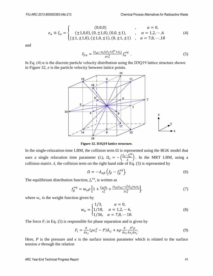
FIU-ARC-2013-800000393-04b-213 Chemical Process Alternatives for Radioactive Waste
ARC Year-End Technical Progress Report 41
{
(4)
and
(5)
In Eq. (4) α is the discrete particle velocity distribution using the D3Q19 lattice structure shown
in Figure 32, e is the particle velocity between lattice points.
Figure 32. D3Q19 lattice structure.
In the single-relaxation-time LBM, the collision term is represented using the BGK model that
uses a single relaxation time parameter (), (
) . In the MRT LBM, using a
collision matrix Λ, the collision term on the right hand side of Eq. (3) is represented by
( ) (6)
The equilibrium distribution function, fαeq
, is written as
[
] (7)
where wα is the weight function given by
{
(8)
The force Fi in Eq. (5) is responsible for phase separation and is given by
. (9)
Here, P is the pressure and κ is the surface tension parameter which is related to the surface
tension σ through the relation
x
y
z
FIU-ARC-2013-800000393-04b-213 Chemical Process Alternatives for Radioactive Waste
ARC Year-End Technical Progress Report 42
∫(
)
(10)
where r is the direction of integration normal to the interface. The force is expressed by Lee
and Lin [36] as
(
) (11)
is the excess free energy at the interface over the bulk free energies and is obtained from an
equation of state (EOS) expressed as follows:
( )
(12)
where is a constant and and
are densities of gas and liquid phases at saturation,
respectively. This EOS results in a density profile given by
(
) (13)
where z is the spatial location normal to the interface and D is the interface thickness.
The constant along with κ can control D and σ through the relation
(
)√
(14)
and
(
)
√ (15)
The forcing term that also appears in Eq. (5) is introduced to represent the effect
of surface molecules where is the parameter that determines whether the solid surfaces act
attractive or repulsive. In addition, the gravitational force is implemented in Eq. (5) via the
force term where stands for the gravitational acceleration vector.
The evolution equations given above for the particle density distribution function is mapped into
the moment space by multiplying the terms in Eq. (3) with the transformation matrix T
⌊⟨ | ⟨ | ⟨ | ⟨ | ⟨ | ⟨ | ⟨ | ⟨ | ⟨ |
⟨ | ⟨ | ⟨ | ⟨ | ⟨ | ⟨ | ⟨ | ⟨ | ⟨ | ⟨ |⌋ (16)
where
| ⟩ | | (17)
| ⟩ | | (18)
| ⟩ | | | |
(19)
| ⟩ (20)

FIU-ARC-2013-800000393-04b-213 Chemical Process Alternatives for Radioactive Waste
ARC Year-End Technical Progress Report 43
| ⟩ ⌊ | | ⌋ (21)
| ⟩ (22)
| ⟩ ⌊ | |
⌋ (23)
| ⟩ (24)
| ⟩ ⌊ | | ⌋ (25)
| ⟩ | |
(26)
| ⟩ | | (
| | ) (27)
| ⟩
(28)
| ⟩ | | (
) (29)
| ⟩ (30)
| ⟩ (31)
| ⟩ (32)
| ⟩ (
) (33)
| ⟩ (
) (34)
| ⟩ (
) (35)
The resulting evolution equation in moment space takes the form
(
) (36)
where
(37)
(38)
(39)
and
(40)
The equilibrium distribution function in moment space is written as
⌊
⌋ (41)
where the equilibrium distributions of the moments are given by
(42)
(43)

FIU-ARC-2013-800000393-04b-213 Chemical Process Alternatives for Radioactive Waste
ARC Year-End Technical Progress Report 44
(44)
(45)
(46)
(
(
)) (47)
(48)
(
) (49)
( ) (50)
( ) (51)
(52)
(53)
(54)
(55)
(56)
In the works of d’Humieres et al. [37], the constants in Eqs. (42-56) are selected as wε = 0, wεj = -
475/63 and wxx = 0 for single-phase flows; however, in this work we follow the selection of
Premnath and Abraham [38] used in their MRT LBM for multiphase flows where wε = 3, wεj = -
11/2 and wxx = -1/2.
The collision matrix in the moment space, , is given as
[ ] (57)
The diagonal elements are inverses of relaxation times for the distribution functions in the
moment space, , and they are used to relax the equilibrium distribution functions in the
moment space, In this work, the diagonal elements are selected as a combination of the
values reported by d’Humieres [37] and Premnath and Abraham [38] as
[
] (58)
The parameters s10, s12 and s14-16 are related to the single relaxation time, τ, in the single-
relaxation-time LBM and are used to determine the viscosity,
(
) and the Reynolds
number, .
As discussed in Lee and Lin [36], it is possible to compute the hydrodynamic variables of
interest such as local density ρ, velocity u, and pressure P, from . This approach, however, is
prone to numerical instabilities due to the steep density gradients involved in the computation of
the source term . Therefore, a separate distribution function g is introduced to compute
pressure and momentum. We denote in the lattice velocity direction α as . A pressure
function p is also defined, which varies smoothly across the interface. It is related to the actual
pressure P through

FIU-ARC-2013-800000393-04b-213 Chemical Process Alternatives for Radioactive Waste
ARC Year-End Technical Progress Report 45
(59)
In the bulk phase, as density gradients are nearly zero. Use of p in the momentum
equation increases the stability of the scheme at high density ratios. This definition of P and the
choice of D in Eq. (13) are critical to the capability of the model to simulate high density ratios.
Based on the definition of p in Eq. (39), Eq. (9) for may be re-arranged as
(
) (60)
However, within this framework of the MRT model, the pressure evolution equation must now
be formulated to have a non-diagonal collision matrix.
To develop an evolution equation for pressure in moment space that is similar to Eq. (26), Lee
and Lin proposed
(
) (61)
where
(62)
(63)
and
(64)
From Eq. (41), the total derivative of can be written as
(65)
which can be simplified to
(66)
where
(67)
[ ( ) ]
(68)
and

FIU-ARC-2013-800000393-04b-213 Chemical Process Alternatives for Radioactive Waste
ARC Year-End Technical Progress Report 46
( ) (69)
To express Eq. (49) as a function of we define
(
) (70)
From this we get the following pressure evolution equation in moment space as
( ) (71)
The macroscopic properties of density, momentum and pressure are obtained from the following
relations:
∑
(72)
∑
[
(
)
(
)]
(73)
∑
(74)

FIU-ARC-2013-800000393-04b-213 Chemical Process Alternatives for Radioactive Waste
ARC Year-End Technical Progress Report 47
RESULTS
In the first numerical test case presented here, the wall adhesion boundary condition
implemented in the LBM code was evaluated for accuracy. The force on the solid surfaces ( )
was made to repel or attract the liquid phases depending on the sign of the Kw parameter. In order
to test the performance of the implementation of this forcing term, a numerical problem was
generated in the computer where a semi-circular droplet was placed on a flat solid surface in a
computational domain filled with a lighter medium. Under a zero gravitational field, the initial
droplet was left to stabilize. Depending on the value and sign of the Kw parameter, the initial
contact angle of the droplet (90) was expected to converge to a value larger or smaller than 90.
Figure 33(a) shows that for a value of Kw = 0.001, the contact angle of the droplet is 77:5 while
Figure 33(b) shows that for Kw = -0.001 the contact angle obtained becomes 102:5. The initial
results indicated that the forcing term implemented in the LBM code could simulate the effects
of hydrophobic and hydrophilic surfaces.
(a) Kw > 0 results in good wetting where < 90° is obtained once the droplet
stabilizes.
(b) Kw < 0 results in partial wetting where > 90° is obtained once the droplet
stabilizes.
Figure 33. Evolution of droplet on a flat surface under hydrophilic or hydrophobic conditions.
Next, the 3D LBM code was utilized to investigate the motion of buoyant bubbles and droplets
in various configurations where the geometry was simple. In these cases the fluids to be
simulated was placed in a box where the sides were specified to be either a periodic boundary or
a solid surface. No inlet and outlet flow boundaries were used. The cases studies included

FIU-ARC-2013-800000393-04b-213 Chemical Process Alternatives for Radioactive Waste
ARC Year-End Technical Progress Report 48
collision of a droplet with a solid surface and on a wet surface. The droplet shown in Figure 34
was released at a certain height close to the bottom wall with zero initial velocity. The droplet
was observed to change shape during the collision process and then attain an ellipsoidal shape
once stabilized. In the case of a wet surface, the droplet was observed to mix into the liquid layer
covering the bottom wall surface. We also tested the code in handling a large number of bubbles
in motion in an open domain under the effect of buoyancy. The first image in Figure 36 shows
the initial configuration of bubbles of equal size placed at zero initial velocity in a liquid box.
The second and third images are obtained as the bubbles rise due to the buoyancy effect. It was
observed that the bubbles at the middle region of the domain rose at a slower speed and were
able to maintain their shapes as compared to the outer bubbles which had a faster rising speed
and collided with surrounding bubbles and formed larger ones.
(a) T=7 (b) T=15 (c) T=28
Figure 34. Collision of a droplet on a solid surface.
(a) T=7 (b) T=15 (c) T=28
Figure 35. Collision of a droplet on a wet surface.

FIU-ARC-2013-800000393-04b-213 Chemical Process Alternatives for Radioactive Waste
ARC Year-End Technical Progress Report 49
Figure 36. Evolution of an array of bubbles rising in an unconfined geometry.
Geometry importing to the LBM
The simulations so far have used simple geometries with rectangular plains in 2D and boxes in
3D. In real-life applications such as the bubble generation in double-shell tanks or mixing of
HLW in tanks with cooling coils, the solid structures such as pipes and tank walls etc. play an
important factor in the behavior of the multiphase flow in these environments. Therefore, during
this fiscal year, FIU investigated options to represent complex geometries in the LBM
framework accurately and efficiently. The ultimate goal was to import an output file from a
computer-aided drawing (CAD) software such as Solidworks into the LBM code. This requires a
process called ‘voxelation’ where the three-dimensional volume-elements, voxels, are used to
represent the geometry on the structured grid of LBM similar to the bitmap representation of
two-dimensional image data. The fluid and solid nodes take either the value of zero or one to be
distinguished in the LBM code once the voxelation process is finished.
FIU worked with Oak Ridge National Laboratory (ORNL) related to this topic where two
students have studied the CartGen procedure being developed at ORNL for the purpose of
representing the complex nuclear reactor parts in the Pratham LBM code ORNL is developing
for single-phase turbulent flow simulations. The CartGen method is currently under development
and has given some issues when the geometry to be voxelated had too many corners. Therefore
FIU has chosen to use the Binvox algorithm developed at Princeton University
(http://www.cs.princeton.edu/~min/binvox/). Using this simple code, FIU were able to convert
STL files obtained from Solidworks software into a RAW format which the LBM code were able
to integrate. A separate subroutine in the 3D LBM code has been written for this purpose. A few
examples of this procedure is shown in the following figure.
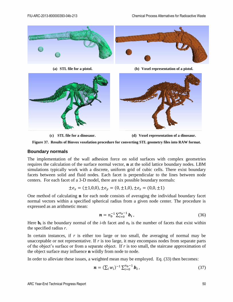
FIU-ARC-2013-800000393-04b-213 Chemical Process Alternatives for Radioactive Waste
ARC Year-End Technical Progress Report 50
(a) STL file for a pistol. (b) Voxel representation of a pistol.
(c) STL file for a dinosaur. (d) Voxel representation of a dinosaur.
Figure 37. Results of Binvox voxelation procedure for converting STL geometry files into RAW format.
Boundary normals
The implementation of the wall adhesion force on solid surfaces with complex geometries
requires the calculation of the surface normal vector, n at the solid lattice boundary nodes. LBM
simulations typically work with a discrete, uniform grid of cubic cells. There exist boundary
facets between solid and fluid nodes. Each facet is perpendicular to the lines between node
centers. For each facet of a 3-D model, there are six possible boundary normals:
One method of calculating n for each node consists of averaging the individual boundary facet
normal vectors within a specified spherical radius from a given node center. The procedure is
expressed as an arithmetic mean:
∑
(36)
Here bi is the boundary normal of the i-th facet and nb is the number of facets that exist within
the specified radius r.
In certain instances, if r is either too large or too small, the averaging of normal may be
unacceptable or not representative. If r is too large, it may encompass nodes from separate parts
of the object’s surface or from a separate object. If r is too small, the staircase approximation of
the object surface may influence n wildly from node to node.
In order to alleviate these issues, a weighted mean may be employed. Eq. (33) then becomes:
∑ ∑ (37)

FIU-ARC-2013-800000393-04b-213 Chemical Process Alternatives for Radioactive Waste
ARC Year-End Technical Progress Report 51
The weighting term is defined as:
⁄ where di is the distance between nodes (i.e.
the center node and the node with normal bi). γ determines the strength of the weighting. For γ
= 0 there is equal weighting for all nodes, thus reducing back to eq. (33). This algorithm was
used to calculate surface normals over a cylinder. The results can be seen below.
Figure 38. 3D Normal vectors for a cylinder.
Simulations with complex geometries
In the following figures, the LBM simulations that included the voxelation process for geometry
import is shown. This includes the motion of a droplet in a constricted channel under inertial
flow and buoyant gas release event in a simplified waste tank. The cases studied allowed us to
observe the effect of structures on the two phases. In the case of the constricted channel problem
presented in Figure 39, the circular droplet retained an elongated shape after it passed through
the constriction. The droplet slows down at the constriction and the time when the droplet leaves
the domain at the exit was affected by the wall surface adhesion coefficient .

FIU-ARC-2013-800000393-04b-213 Chemical Process Alternatives for Radioactive Waste
ARC Year-End Technical Progress Report 52
T=0
T=40
T=60
T=70
Figure 39. Droplet flow in a constricted channel with attractive walls (left) and repulsive walls (right).
A simulation has also been conducted involving buoyant bubble rise in a complex geometry
environment in order to evaluate the performance of the LBM code with the geometry import
and contact line dynamics features for a case that may be relevant to the DOE waste tank
operations. The simulations aimed to test the applicability of the LBM simulations for the
estimation of buoyant displacement gas release event that may occur in the DSTs. To mimic the
complex geometry of a waste tank with the cooling structures as shown in Figure 40 for a tank in
Savannah River Technology Laboratory, FIU generated a Solidworks drawing for the cross-
section of a tank that has similar features.

FIU-ARC-2013-800000393-04b-213 Chemical Process Alternatives for Radioactive Waste
ARC Year-End Technical Progress Report 53
Figure 40. Cooling coils in Tank 1 in SRNL on the left and the cross section of a similar geometry in
Solidworks on the right.
Since the LBM code doesn’t have the feature of a bubble generation mechanism built-in, we
placed 7 bubbles of equal size at the bottom of the tank at a density ratio of 1 to 10 compared to
the surrounding liquid. Once the gravity is turned on and the bubbles were let to rise, it was
observed that some bubbles were restricted to rise by the horizontal pipe structures represented in
the domain as circular objects which delayed the increase of the gas phase in the head-space.
Others have come together and formed larger bubbles. The influence of the vertical pipe was
found to be less compared to the horizontal pipes represented by the circular solid structures in
the domain. The figure below shows the change of the interface of the bubbles as they rise as
well as the fluid velocity vectors colored with velocity magnitude. Although the simulation
domain was a simple representation of the real complex environment in a waste tank, the
potential of the LBM code was proven for the understanding of bubble entrapment and release in
the multiphase flow environment in nuclear waste tanks. FIU will try to get the CAD file of such
a tank geometry and conduct larger scale simulations including the full tank.
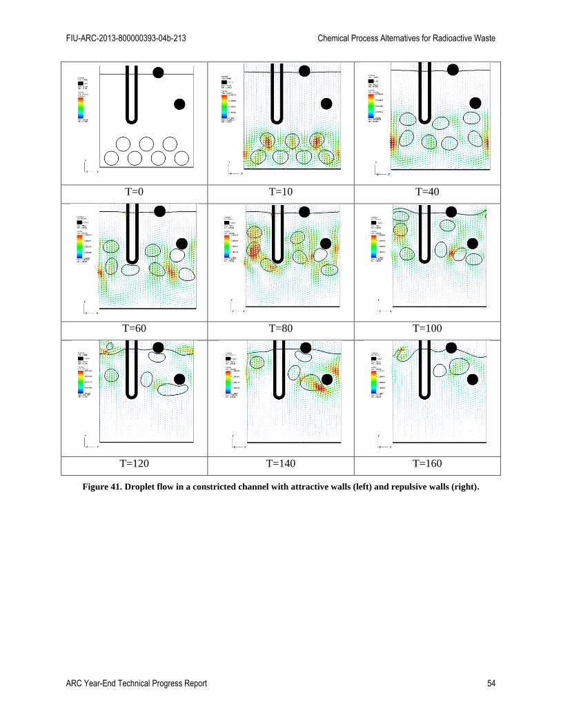
FIU-ARC-2013-800000393-04b-213 Chemical Process Alternatives for Radioactive Waste
ARC Year-End Technical Progress Report 54
T=0 T=10 T=40
T=60 T=80 T=100
T=120 T=140 T=160
Figure 41. Droplet flow in a constricted channel with attractive walls (left) and repulsive walls (right).

FIU-ARC-2013-800000393-04b-213 Chemical Process Alternatives for Radioactive Waste
ARC Year-End Technical Progress Report 55
CONCLUSIONS
In this work, we presented a concise literature review on modeling turbulent flows and non-
Newtonian flows with LBM. Our study revealed that the extension of the lattice Boltzmann
method for the simulation of complex fluid flows including turbulent flows and non-Newtonian
fluids is possible via various approaches, although a well-established method has not yet been
achieved. In comparison to the turbulence models proposed for LBM, the incorporation of non-
Newtonian fluid properties in the LBM simulations have been presented more consistently. The
LES-LBE applications show more promise in terms of turbulence modeling with LBM due to its
simpler implementation and higher accuracy over two-equation models. It should be noted that
the authors were not able to find an application of LBM for turbulent flows in a multiphase flow
configuration; therefore, the future LBM task at FIU that aims to simulate turbulent flows in
nuclear tanks with multiple phases of fluids would be a challenging and scientifically important
effort, especially if both of the subgrid models and Bingham plastic effects could be incorporated
simultaneously in the viscosity definition of the lattice Boltzmann equation.
The formulation of a Multiple Relaxation Time LBM based on the Lee and Lin multiphase
model was presented for dynamic bubbles and droplets in three dimensional domains with
complex geometries and under the effect of wall adhesion and gravitational forces. Numerical
cases of moving bubbles and droplets in confined and open computational domains have been
presented and the capability of the method to simulate dynamic interface tracking of the fluid
interface in contact with the solid surfaces has been shown. The numerical method based on a
multiphase LBM established with this research effort was able to provide promising preliminary
results for a case that represents similar piping features of a DOE nuclear waste tank. However,
further improvement of the method needs to be performed with appropriate inlet and outlet
boundary conditions to simulate flows with injections and mixing of fluids.
Future work will include implementation of a turbulence model for injection type flows as well
as modifying the viscosity definition in LBM to simulate non-Newtonian fluids. The LES-LBM
will be the approach to follow for the turbulent flow simulations with LBM; however, the
cascade-LBM will also be investigated if time permits which claims to not necessitate a separate
turbulence model within the LBM framework. The extension of the LBM code to non-
Newtonian flow modeling will also be conducted in the next fiscal year especially related to
Bingham plastic fluids that are found in the DOE waste tanks.

FIU-ARC-2013-800000393-04b-213 Chemical Process Alternatives for Radioactive Waste
ARC Year-End Technical Progress Report 56
REFERENCES
1. Fox, Robert W and McDonald, Alan T. Introduction to Fluid Mechanics. New York : John
Wiley & Sons, Inc., 1994.
2. Kolmogorov., A. The equations of turbulent motion in an incompressible fluid. Izv. Sci.
USSR Phys. 1942, Vol. 6, pp. 56-58.
3. Bamberger , J A, et al. Technical Basis for Testing Scaled Pulse Jet Mixing Systems for
Non-Newtonian Slurries. s.l. : Battelle, 2005. WTP-RPT-113.
4. Latt, J. Hydrodynamic limit of lattice Boltzmann equations. Geneva, Switzerland :
University of Geneva, 2007. 3846.
5. General circulation model of the atmosphere. Smagorinsky, J. 1963, Mon. Wheather Rev.,
Vol. 91, pp. 99-164.
6. Comparison of spectral method and lattice Boltzmann simulations of two-dimensional
hydrodynamics. Martinez, D O, et al. 1994, Physics of Fluids, pp. 1285-1298.
7. Two-dimensional turbulence with the lattice Boltzmann equation. Benzi, R and Succi, S.
1990, J. Phys. A, Vol. 23, pp. L1-5.
8. Recent advances in lattice Boltzmann computing. Qian, Y H, Succi, S and Orszag, S A.
1995, Annu. Rev. Comp. Phys., Vol. 3, pp. 195-242.
9. The lattice-Boltzmann equation - a new tool for computational fluid dynamics. Succi, S,
Benzi, R and Higuera, F. 1991, Vol. 47, pp. 219-230.
10. Recovery of the Navier-Stokes equations using a lattice-gas Boltzmann method. Chen, H,
Chen, S and Matthaeus, W H. 1992, Phys. Rev. A, Vol. 45, pp. R5339-42.
11. Lattice Boltzmann and spectral simulations of non-linear stability of Kolmogorov flows.
Trevino, C and Higuera, F. 1994, Vol. 40, pp. 878-90.
12. Extended self-similarity in numerical simulations of three-dimensional anisotropic
turbulence. Benzi, R, Struglia, M V and Tripiccione, R. 1996, Phys. Rev. E, Vol. 53, pp.
R5565-68.
13. Direct and large-eddy simulation of turbulent fluid flow using the lattice-Boltzmann
scheme. Eggels, J GM and Somers, J A. 1996, Int. J. Heat Fluid Flow, Vol. 17, pp. 307-23.
14. Reynolds number scaling of cellular automaton hydrodynamics. Orszag, S A and Yakhot,
V. 1986, Phys. Rev. Lett., Vol. 56, pp. 1691-93.
15. A lattice Boltzmann subgrid model for high Reynolds number flows. Hou, S, et al. 1996,
Fields Inst. comm., Vol. 6, pp. 151-66.
16. Direct simulation of fluid flow with cellular aytomata and the lattice Boltzmann equation.
Somers, J A. 1993, Applied Sci. Res., Vol. 51, pp. 127-33.
17. Direct and large-eddy simulation of turbulent fluid flow using the lattice-Boltzmann
scheme. Eggels, J G.M. 1996, Int. J. Heat and Fluid Flow, pp. 307-323.
18. Derksen, J and Van den Akker, H. Parallel Simulation of Turbulent Fluid Flow in a Mixing
Tank. [ed.] P Sloot, M Bubak and B Hertzberger. High-Performance Computing and
Networking. s.l. : Springer Berlin Heidelberg, 1998, pp. 96 - 104.
19. Large Eddy Simulations on the Flow Driven by a Rushton Turbine. Derksen, J and Van den
Akker, H E.A. 2, 1999, AIChE Journal, Vol. 45, pp. 209-221.
20. Krafczyk, M. Gitter-Boltzmann-Method: Von der Theorie zur Anwendung. Munich,
Germany : s.n., 2001.

FIU-ARC-2013-800000393-04b-213 Chemical Process Alternatives for Radioactive Waste
ARC Year-End Technical Progress Report 57
21. LARGE-EDDY SIMULATIONS WITH A MULTIPLE-RELAXATION-TIME LBE
MODEL. Krafczyk, M, Tolke, J and Luo, L-S. 1&2, 2003, International Journal of Modern
Physics B, Vol. 17, pp. 33-39.
22. Incorporating Turbulence Models into the Lattice-Boltzmann Method. Teixeira, C M. 8,
1998, International Journal of Modern Physics C, Vol. 9, pp. 1159-1175.
23. Challenges in lattice Boltzmann computing. Succi, S, Amati, G and Benzi, R. 1995, J. Stat.
Phys., Vol. 81, pp. 5-16.
24. Lee, K P, et al. Waste Feed Delivery Mixing and Sampling Program Simulant Definition
for Tank Farm Performance Testing. Richland, WA : Washington River Protection
Solutions, 2012. RPP-PLAN-51625.
25. Gauglitz, P A, et al. The Role of Cohesive Particle Interactions on Solids Uniformity and
Mobilization During Jet Mixing: Test Recommendations. Richland, WA : Pacific
Northwest National Laboratory, 2010. PNNL-19245.
26. Gauglitz, P A, et al. Mechanisms of Gas Bubble Retention and Release: Results for
Hanford Waste Tanks 241 S 102 and 241 SY 103 and Single Shell Tank Simulants.
Richland, WA : Pacific Northwest National Laboratory, 1996. PNNL-11298.
27. Non-Newtonian Flow (Through Porous Media):A Lattice-Boltzmann Method. Aharonov, E
and Rothman, D H. 8, 1993, Geophysical Research Letters, Vol. 20, pp. 679-682.
28. Lattice Boltzmann method for non-Newtonian (power-law) fluids. Gabbanelli, S, Drazer, G
and Koplik, J. 2005, Physical Rewview E, Vol. 72, pp. 046312-1.
29. A second-order accurate lattice Boltzmann non-Newtonian flow model. Boyd, J, Buick, J
and Green, S. 2006, Journal of Physics A: Mathematical and General, Vol. 39, pp. 14241-
14247.
30. Electroosmotic flow of non-Newtonian fluid in microchannels. Tang, G H, et al. 2009,
Journal of Non-Newtonian Fluid Mechanics, Vol. 157, pp. 133-137.
31. A numerical method for incompressible non-Newtonian fluid flows based on the lattice
Boltzmann method. Yoshino, M, et al. 2007, J. Non-Newtonian Fluid Mechanics, Vol. 147,
pp. 69-78.
32. Flows of Materials with Yield. Papanastasiou, T C. 5, 1987, Journal of Rheology, Vol. 31,
pp. 385-405.
33. Lattice Boltzmann modeling of Bingham plastics. Wang, C-H and Ho, J-R. 2008, Physica
A, Vol. 387, pp. 4740-4748.
34. Bingham fluid simulation with the incompressible lattice Boltzmann model. Tang, G H, et
al. 2011, Journal of Non-Newtonian Fluid Mechanics, Vol. 166, pp. 145-151.
35. Multiple-relaxation-time lattice Boltzmann model for generalized Newtonian fluid flows.
Chai, Z, et al. 2011, Journal of Non-Newtonian Fluid Mechanics, Vol. 166, pp. 332-342.
36. A stable discretization of the lattice Boltzmann equation for simulation of incompressible
two-phase flows at high. Lee, T., & Lin, C.-L. 2005. Journal of Computational Physics,
206, 16-47.
37. Multiple-relaxation-time lattice Boltzmann models in three dimensions. D. D'Humières, I.
Ginzburg, M. Krafczyk, and P. & Luo, L.-S. Lallemand. 2002. Royal Society of London
Philosophical Transactions Series A, vol. 360, p. 437.
38. Three-dimensional multi-relaxation time (MRT) lattice-Boltzmann models for multiphase
flow. K. N. Premnath and J. Abraham. 200.7 Journal of Computational Physics, vol. 224,
pp. 539-559.

FIU-ARC-2013-800000393-04b-213 Chemical Process Alternatives for Radioactive Waste
ARC Year-End Technical Progress Report 58
TASK 15: EVALUATION OF ADVANCED INSTRUMENTATION
NEEDS FOR HLW RETRIEVAL
EXECUTIVE SUMMARY
As the DOE’s Hanford Site begins preparations for the transfer of high-level radioactive waste
(HLW) from the double-shell tanks (DST) to the Waste Treatment and Immobilization Plant
(WTP), the influence of waste feed consistency on the waste stabilization process – and final
stabilized waste form – is currently under analysis. In order to characterize feed consistency
prior to transfer, a suite of instrumentation will be required to monitor the waste preparation and
mixing process in real time. FIU has focused its instrumentation efforts on identifying
improvements to the in-situ, near-real time monitoring of the mixing process. Specifically, this
project has identified innovative technologies applicable for in-tank monitoring during the
mixing process.
After the current technology baseline plan and previous research efforts were reviewed, FIU
performed an extensive literature and technology search for applicable systems that could
provide waste parameters within the HLW tank environment. The literature search focused on
available methodologies for in-situ analysis of slurries, emulsions and suspensions applied in all
industries. In particular, the monitoring of bulk density and/or particle
concentration/characteristics measurements was the focus of the search. For the technology
search, vendors of applicable techniques were identified and contacted. The searches resulted in
several academic, commercial and governmental reports/articles applicable to the monitoring
needs of the HLW tanks. Instrumentation specifications were collected and reviewed to identify
the technology capabilities and limitations. These capabilities were also used for a comparative
analysis between technologies. Based on the information, all the technologies were down
selected to five applicable systems/methods that could provide useful information if deployed in
a HLW tank. The five applicable methods applicable to the in-situ monitoring of the waste feed
consistency were focused beam reflectance measurement (FBRM), optical back-reflectance
measurement (ORM), ultrasonic spectroscopy (USS), Lamb/Stoneley wave viscosity
measurement, and vibration-based densitometers. Based on literature results and commercial
options, the ultrasonic and vibration-based techniques showed the most promise for developing a
technology that could be used for in-situ measurements within the aggressive environment of a
HLW tank. Specifically, the vibration-based densitometers and USS systems could provide
information on the density and concentrations of the mixed slurry. These techniques had the
potential to be engineered for monitoring at various depths within the tank.
In order to evaluate a technology, the USS was tested on an array of slurries, and the density
compared to a commercially available density meter that utilizes an accurate and repeatable
technique for density measurement. A setup was conceived that allowed the testing of the USS
and a commercially-available Coriolis mass flow meter side-by-side. The setup used a 10-gallon
tank for agitation of the simulated slurry mixtures, with both systems sampling at the same
location; the USS system probe was lowered into the tank, while a pick-up tube was used to
transfer mixture to the Coriolis meter. In addition, the USS was subjected to several tests using a
benchtop setup for more controlled evaluations of its concentration tracking capabilities. Both

FIU-ARC-2013-800000393-04b-213 Chemical Process Alternatives for Radioactive Waste
ARC Year-End Technical Progress Report 59
these systems were subjected to solutions and suspensions that would simulate some of the
physical and rheological properties of the HLW slurry found in AY-102. The simulated slurries
consisted of one to three distinct solids suspended in a water or NaNO3 solution as the
supernatant.
FIU tested the USS between May and October of the previous year with delays associated with
hardware and software issues that plagued the device under evaluation. In August, the system
had to be returned to the vendor as a result of a hardware fault. A new system was sent to FIU in
October, and was used to complete testing. The results indicated that the technology could
provide a measurement of density, but the frequency at which it occurs varies with slurry
characteristics. If one frequency is selected for analysis, the density values vary more than 10%
when compared to the reference value. One major issue that occurred during testing was that the
spectral response profile of the USS system changed between hardware changes, and this was
something that the vendor attributed to an issue with the reference file used for the tests.
In order to address issues with system inconsistency, additional bench-scale tests were performed
at ITS facilities during the first quarter of this performance period. The testing utilized similar
materials, concentration profiles for NaNO3 and solids loading profiles in an attempt to
determine the root cause for the inconsistency of results, as well as to compare the results to the
FIU data. The USS utilized consisted of a through-transmission configuration, which had a
slightly larger transducer than those tested at FIU. The ITS test results indicated good agreement
between the measured and calculated densities for solutions, and certain material and
water/NaNO3 suspension. The technology showed significant variance between the measured
and calculated densities for complex mixtures (multiple solids). This variance was again
attributed to the significant attenuation of the acoustic pulse after traversing the suspension. This
attenuation caused issues in the detection of the correct return echo from the suspensions. With
incorrect detection, the measured density value showed significant errors (> 20%).
Based on the results of the testing at ITS facilities, it is evident that the technology still requires
the following: applied research in the design and selection of the necessary transducers to
provide the needed sensitivity; additional engineering analysis to improve signal acquisition and
detection at low signal levels; and basic research into the influence of complex mixtures that
contain matter that displays an inverse relationship between speed of sound and concentration.
With these limitations, the technology is not at the readiness level required for deployment at the
WTP waste feed mixing tank AY-102. The USS has several technical limitations that must be
addressed before system would be at a TRL readiness level commensurate with a potential
deployment in 2-3 years.

FIU-ARC-2013-800000393-04b-213 Chemical Process Alternatives for Radioactive Waste
ARC Year-End Technical Progress Report 60
INTRODUCTION
The US Department of Energy’s (DOE) Hanford Site is completing development of the Waste
Treatment and Immobilization Plant (WTP), and preparing for the processing of over 54 million
gallons of high-level radioactive waste (HLW). This waste shall be mixed within storage tanks,
transferred to staging tanks, and processed by the WTP for final disposal. As the WTP
development is completed, the window to integrate additional instrumented systems into the
process loop will close. One such area that could benefit from additional instrumentation is the
HLW tanks where this waste is currently stored. These +1M gallons of waste must be mixed into
slurry that can be retrieved via pipelines to other tanks, or to WTP. The ability to characterize
slurry in-tank would greatly optimize the mixing and retrieval processes. After several years of
experience in the development of remote monitors for HLW tanks, FIU has undertaken a task to
evaluate additional characterization and monitoring technologies that could be scaled-up for
deployment inside the HLW tanks at Hanford.
During the 2010 performance period, FIU conducted a literature search for promising
technologies that could be utilized in-situ and provide process engineers with near real-time
information on slurry parameters during the mixing process. In particular, technologies that
could monitor the slurry bulk density were highlighted and reviewed via addition literature
search and screening. The search identified two technologies/methodologies that could be
deployed in a HLW tank, and could provide useful bulk density information at various depths in
the tank. These included a Coriolis-principle based densitometer, and an Ultrasonic
Spectroscopy-based technology (USS). The Coriolis meter utilized was a commercially available
Promass 63F by Endress-Hauser, and the USS was a commercially available system from
Industrial Tomography Systems plc (ITS). FIU evaluated both these technologies in a laboratory
setting with slurry simulants. The technology results were inconclusive; the USS system(s)
showed varying results for the same slurry characteristics. These variations were attributed to a
system performance issue. In order to address these variations, an additional round of testing was
performed at ITS on a bench-scale setup with more controlled suspensions. This report
summarizes the tests performed as well as addresses a timeline for data analysis.
FIU-ARC-2013-800000393-04b-213 Chemical Process Alternatives for Radioactive Waste
ARC Year-End Technical Progress Report 61
EXPERIMENTAL APPROACH
In order to mitigate system issues from affecting the test success, it was determined that the tests
should be performed at ITS facilities. The vendor would be capable of addressing any system
issues during testing, and would follow the test requirements and goals defined by FIU. In order
to collect sufficient information to ensure that the technology could proceed into a prototype
development stage, the tests were divided into two phases: a (1) NaNO3 concentration ladder
phase, and a (2) solids loading ladders tests with different materials. The first phase involved
concentration ladder of aqueous NaNO3 solutions. A mixture was prepared and static (no
mixing) measurements were taken in the cell for the following concentrations: 0.1%, 0.5%, 1%,
2%, 3%, 5%, 7%, 10%, 15%, 20%, 25%, 30%, and 37.5%. For the second phase, distilled water
was used as the continuous phase in aluminum hydroxide, zirconium oxide and stainless steel
mixtures and further on the ultrasonic measurements of the mixtures. Measurements were taken
for the following concentrations (by volume): 0.1%, 0.5%, 1%, 2%, 3%, 5%, 7%, 10%, 15%,
20%, and 25%.
In this test program, the USS was configured in a through-transmission mode. This would
address the expected large attenuation caused by the solids utilized. It is expected that a field
deployable system will have to utilize a through-transmission system in order to address the large
attenuation expected in Hanford's HLW tanks . All measurements were carried out using a USS
in-line measurement cell in the static and dynamic conditions. The experiments consisted of 10
repeated measurements for each sample. The sample was then removed from the cell for disposal
and new material was added. In the case of sodium nitrate concentration ladder, the spacing
between transducers was set to 22-mm. That spacing was reduced to 10-mm for suspensions
phase. The system was calibrated using deionized water as a reference media. Additional
parameters of the experiment: room temperature, the volume of the sample 350 ml.
FIU-ARC-2013-800000393-04b-213 Chemical Process Alternatives for Radioactive Waste
ARC Year-End Technical Progress Report 62
RESULTS & DISCUSSION
The test report provided by ITS is presented in Appendix A. Analysis of the NaNO3 solutions
show good agreement with the expected wave speed, and agrees with the data collected during
FIU testing. The attenuation data shows that these solutions experience less attenuation than a
water mixture. Analysis of the density measurement for the aluminum hydroxide solid loads
indicates good agreement with the calculated value, even into the 30% concentration. The
measurements collected from the suspensions of zirconium oxide in water showed the inversely
proportional velocity to the concentration of the sample. The complex mixture data showed
significant variations in the density as compared to the calculated value, which indicates
significant attenuation of the ultrasonic pulse.

FIU-ARC-2013-800000393-04b-213 Chemical Process Alternatives for Radioactive Waste
ARC Year-End Technical Progress Report 63
CONCLUSIONS
The results from this final phase of testing indicates that several areas of the technology still
require substantive applied research in order to overcome current limitations. The technology
holds potential as a simplified bulk density and concentration method, but it requires additional
work in order to overcome current commercial design limitations. There are three areas that
require more applied research to overcome the limitation. First, the design and selection of the
necessary transducers to provide the needed sensitivity must be reviewed; the benefits of
advanced piezo-composite transducers can improve signal sensitivity and fidelity. Second,
additional engineering analysis must be performed to improve signal acquisition and detection at
low signal levels. The utilization of higher sensitivity acquisition system, as well as better control
of thermal voltage levels, can improve minimum detectable signal level. Finally, basic
information on the complex mixtures, especially those that contain matter that displays an
inverse relationship between speed of sound and concentration, must be investigated. The
attenuation characteristics at varying spectra of the expected waste stream must be properly
considered when evaluating the response to a broadband ultrasonic pulse.

FIU-ARC-2013-800000393-04b-213 Chemical Process Alternatives for Radioactive Waste
ARC Year-End Technical Progress Report 64
TASK 16: COMPUTATIONAL SIMULATION AND EVOLUTION OF HLW PLUGS
EXECUTIVE SUMMARY
Pipeline plug formation is caused by changes in the chemistry and flow patterns within the pipe
transfer system at Hanford. A better understating of the interactions between the chemical
species leading to precipitate formation is required to reduce the risk pipe plugging. A need
exists for a computational tool that can predict plug formation by considering the chemistry
dynamics coupled with fluid particle interactions. The use of Computational Fluid Dynamics
(CFD) software has been explored in the past to predict plug formation [1, 2]. The plugging
mechanism simulated was settling of solids. Even though the efforts were promising, the models
lacked incorporation of chemical reactions kinetics. Hence, a new task was initiated as part of
Florida International University’s research efforts to develop a multi-physics model using CFD
software that could simulate the coupled flow and chemistry kinetics and aid in understanding
the plug formation process.
A literature review was conducted using major search engines to advance the plug formation
knowledgebase, with specific applications to the Hanford Site. The review focused on four
areas: (i) Overview of the waste transfer system at Hanford, (ii) Plugging mechanisms and waste
transfer dynamics, (iii) Current analysis tools-capabilities and limitations, and (iv) Use of
computational fluid dynamics (CFD) modeling to predict the plug formation process.
Several models were evaluated simulating single phase and multi-phase reacting flow kinetics
using Comsol Multiphysics 4.3bTM
for laminar flow. The study of reacting flow involved
investigating how the flow affected the chemical reaction process. For the single phase
simulations, the baseline model consisted of a reacting flow entering a horizontal pipe section.
The influence of bends on the reacting flow field was analyzed by adding a 90° elbow and a
straight pipe section to the baseline model. The evolution of species was investigated as they
were transported through the pipe. The velocity and concentration profiles were plotted to
analyze the effect of flow field on the chemical reaction process. For the multi-phase
simulations, the model consisted of a mixture flow (10% volume fraction of clay dispersed in
water) through a horizontal pipe. The settling of solids along the pipe length was studied and the
volume fractions of the continuous phase (water) and the dispersed phase (clay) were plotted.
The results from the single phase and multi-phase simulations demonstrated the ability of
Comsol Multiphysics 4.3bTM
to simulate coupled flow chemistry models. Future work will
include modeling single phase and multi-phase reacting flow at turbulent velocity, coupling
chemical reactions to the multi-phase flow and incorporating dynamics processes such as
precipitation, particle agglomeration, particle breakup to the models to gain a better
understanding of reaction kinetics that lead to plug formation.

FIU-ARC-2013-800000393-04b-213 Chemical Process Alternatives for Radioactive Waste
ARC Year-End Technical Progress Report 65
INTRODUCTION
Hanford’s waste is a chemically complicated system. The main goal of Hanford’s waste transfer
system is to transfer such waste without plugging the transfer pipelines. The current tools that are
used currently to support this objective include the Environmental Simulation Program (ESP)
and critical velocity correlations. ESP is used to estimate the initial waste compositions and
solids volume fraction and critical velocity correlations are then used to calculate flow velocities
and pressure drops for waste transfers. The tools are used in tandem to mitigate the risk of
plugging by ensuring that the waste meets the waste acceptance criteria (WAC).
Despite such efforts, several lines have plugged during the waste transfer process at Hanford.
The plugging has been attributed to two main factors: precipitation/crystallization and settling of
solids. Both ESP and critical velocity correlations address only one plugging mechanism-
settling of solids. The tools do not account for precipitation dynamics. Computation fluid
dynamics (CFD) models developed by others (MSU DIAL and PNNL) also do not incorporate
chemical interactions and precipitation kinetics.
Changes in the chemical environment and fluid dynamic forces can result in dramatic changes in
slurry properties and flow behavior during a transfer. Agglomeration and particle breakup due to
changes in the chemical environment, particle-particle interactions, and precipitation, can result
in waste behaviors that cannot be predicted by considering equilibrium chemistry or fluid flow
alone.
A multi-physics model that accounts for waste chemistry coupled with fluid dynamics was
proposed by FIU to address the identified shortcomings. In this report, results of the single phase
reacting flow models and multi-phase mixture model are presented. The CFD model couples the
two components: (1) Flow Interface and (2) Chemical Reaction Interface. The flow interface is
solved first and its calculated velocity field is used as a model input for the chemical reaction
interface to study the evolution of chemical species. The CFD software used for the simulations
is Comsol Multiphysics 4.3bTM
.
The outline of the report is given as follows: First, the findings of a comprehensive literature
review are presented. The review focuses on four areas: (i) Overview of the waste transfer
system at Hanford, (ii) Plugging mechanisms and waste transfer dynamics (iii) Current analysis
tools-capabilities and limitations and (iv) CFD modeling to predict the plug formation process.
Then, the single phase and multi-phase simulations models are discussed and the results obtained
are reported. Finally, conclusions are drawn and discussions for future work are presented.
Background
History of Plugged Pipelines
Plugging was first observed during the cross-site transfer operations conducted in the late 1950s
and early 1960s [3]. The reason for the plugging was attributed to insufficient heating of the
waste during transfer. As the slurry cooled, it was believed that solids precipitated out of solution
and began to accumulate on the pipe walls. Eventually, the solids would block the pipe. The
plug was blown out of the pipe with a 200 psi flush fluid. A more thorough investigation of line
plugging event was documented in 1978 by [4] during which formation of tri-sodium phosphate

FIU-ARC-2013-800000393-04b-213 Chemical Process Alternatives for Radioactive Waste
ARC Year-End Technical Progress Report 66
crystals was reported. The crystals impeded the flow within the pipe and completely plugged the
pipeline. The formation of these phosphate crystals was studied extensively in the 1980s. 2,3
Several pipeline plugs were observed during salt-well transfers and a majority of them were
attributed to precipitation of sodium phosphate [5]. In each case, the transfer of the waste was
suspended, and the pipeline was not flushed with water. The line from tank BY-103 was
pumping waste without dilution. Due to a flammable gas concern, the pumping was shut off
without flushing the line. Some month’s later a plug was discovered in the pipeline. The plug
could not be broken and the line was abandoned. The transfer line from tank SX-104 was
pumping waste with ineffective dilution. The pumping was stopped temporarily. On restart of
the transfer operations, a plug was discovered in the unheated jumper. The plug was eventually
broken using a hot water flush. Pumping was stopped in line from tank U-103 and the line was
not flushed for over 24 hours. On restart, the plug was observed in a non-heat traced flexible
jumper. A jumper was pulled to break the U-103 plug. In an effort to avoid further plugs, the
modifications such as larger flex jumpers and additional heat tracing were made to the transfer
system.
Plugging Mechanisms
The primary mechanisms that contribute to transfer line plugging at Hanford were identified
from various reports [6, 7, and 8] and are as follows:
(a) Chemical Instability (precipitation, crystallization)
(b) Settling of solids – including hydrodynamic instability
Depending on the mechanism, plugging or its onset may result in a change in the particle size
distribution or the density of the slurry. In addition, the onset of pipeline plugging may also lead
to an increase in pressure drop in the transfer lines.
Chemical instability: Chemical instability during waste transfers results is a phase change (from
liquid to solid) initiated due to drop in temperature, changes in local concentration or mixing and
pumping of wastes that are not in equilibrium. The solid phase precipitates or crystallizes
depending on the solubility characteristics of the dissolved multiple species of the waste, their
chemical interaction, and temperature. The solids may precipitate out of the solution and
accumulate along the pipe walls. The pipe walls would then serve as a nucleation site where the
solids would nucleate and grow rapidly and eventually form an interlocking needle-like crystal
network. The needle-like crystal network then impedes the flow within the pipe and commences
the formation of the plug. At Hanford, the crystallization or precipitation process has mainly
been observed in phosphates-and aluminates-containing supernatant wastes.
2 Internal Letter No. 65453-80-296 by D. L. Herting, “Evaporator Feeds High in Phosphate,”
Rockwell Hanford Operations, Richland, Washington (1980).
3 Internal Memo No. 65124-068-80, by C. H. Delegard. “Viscosity/Cooling Data for Tanks
107-S and 105-BX Waste Liquors;’ Rockwell Hanford Operations, Richland, Washington
(1985).

FIU-ARC-2013-800000393-04b-213 Chemical Process Alternatives for Radioactive Waste
ARC Year-End Technical Progress Report 67
Phosphate salts can form needle like crystals at low temperatures (40 to 60 C) at typical
concentrations found in Hanford waste types. The effect of temperature on phosphate crystal
formation was investigated and reported in an internal letter [9]. The author found that at
temperatures above 55°C, granular sodium phosphate crystals (Na3PO4.6H2O) were formed and
that at temperatures below 55°C needle like sodium phosphate crystals (Na3PO4.12H2O) were
formed. The main difference between the two forms was differing waters of hydration. The
author made a key observation that “the viscous suspensions of Na3PO4.12H2O needles could be
converted by prolonged agitation to a well-settling mixture composed of 25% settled solids by
volume”, indicating that the gel is shear-thinning, believed to be largely due to alignment of
needle crystals. The author concluded that if a gel of the 12-hydrate crystals were to form a plug
in a pipeline, it would be difficult to impart sufficient energy into the plug to cause shear
thinning and remove the plug. In general, the formation of needle crystals is inhibited at high
temperatures.
The solubility of sodium phosphate is also highly temperature dependent. Sodium phosphate
solubility as a function of temperature and sodium ion concentrations was investigated [10]. He
found that solubility of phosphate is strongly temperature dependent with a linear dependence on
sodium ion concentration at 50°C and 60°C. For example at 50°C, at 8 M sodium, the phosphate
solubility was reported as approximately 0.3 M increasing to 0.45 M at 5 M sodium. At 40°C,
the data was much less dependent on sodium ion concentration, and indicated a phosphate
solubility of approximately 0.1 M to 0.15 M above 5 M sodium. At 20°C, the solubility of
phosphate was noted to be in the range of 0.03 M to 0.08 M. Hence, it can be concluded that
phosphate is more soluble at higher temperatures.
The above discussed findings clearly illustrate the potential difficulties that can be encountered
while handling phosphate waste. To avoid transfer problems with phosphate containing waste
[11] recommended the following precautions: First, the tank waste should not be heated prior to
the transfer. Second, the waste should not be allowed to cool during the transfer. Third, the
waste should be kept moving during the transfer.
In addition to phosphate crystals, the precipitation of aluminates also has the potential to plug
slurry transfer systems at Hanford. Aluminates can precipitate by at least two mechanisms: the
formation of amorphous or crystalline solid phases such as gibbsite, and the formation of sodium
aluminate. The solubility of aluminum was investigated as function of high ionic strengths by
[12]. The author presented a phase map (sodium hydroxide vs. sodium aluminate) as shown in
Figure 42 and found that the solubility of aluminum hydroxide was greatly increased at higher
ionic strengths. In solutions with high sodium hydroxide concentrations (above 2 M), it was
found that increasing aluminum concentration would eventually precipitate sodium aluminate
salts. It was also observed that at lower sodium hydroxide levels, an increase in the molar
aluminum concentration resulted in precipitation of aluminum hydroxides.

FIU-ARC-2013-800000393-04b-213 Chemical Process Alternatives for Radioactive Waste
ARC Year-End Technical Progress Report 68
Figure 42. Aluminum solubility as a function of sodium hydroxide [12].
These aluminum hydroxides can take on several forms, including amorphous, gibbsite, and
boehmite. The amorphous form is thought to precipitate out more quickly, sometimes forming
gels that can be problematic during waste transport. The amorphous hydroxide is usually
converted within hours or days into crystalline gibbsite phase. Gibbsite typically forms roughly
spherical-shaped particles that are of colloidal size but have been observed in waste streams as
stable agglomerates [13]. Gibbsite is thought to be relatively common among the waste
aluminum phases and has been observed in samples from Tank 241-SY-103 [14]. Boehmite is
thought to be less common in waste, and had been typically observed in tanks (Tank 241-T-111)
where self-boiling of waste occurred due to high decay heat [15].
One of the control strategies recommended in [16] while handling aluminum rich waste included
avoiding over dilution of aluminum rich supernatant with water as that could shift the waste
composition towards the left hand phase boundary at which gibbsite solids could precipitate.
The use of caustic solution of sodium hydroxide was recommended for dilution rather than
water, to shift the waste composition to the right, away from the gibbsite phase boundary. In the
event of a line plugging by gibbsite precipitation, caustic solution was again recommended to be
used as a flushing fluid to re-dissolve the precipitates and clear the line. Gibbsite precipitation
plugged a U-Farm transfer line during saltwell pumping in 2003. Caustic soak was used to
unplug that line.
Settling of Solids: The presence of precipitates and/or agglomerates increases the solids
concentration and increases viscosity of the slurry. The flow can transition from turbulent to
laminar flow as a result of such changes during transit and the undissolved solids may settle
when the flow velocity is not sufficient to keep them suspended. A moving bed of particles
begins to accumulate during a slurry transport operation. Settling solids in a moving bed of
particles form a stationary bed that eventually fills the pipe and blocks flow. Critical velocity
correlations are used to estimate the minimum velocity to prevent settling of solids.
Source of concern
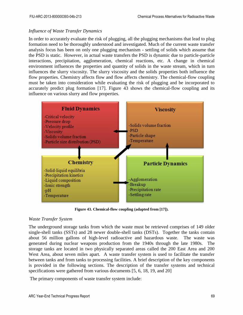
FIU-ARC-2013-800000393-04b-213 Chemical Process Alternatives for Radioactive Waste
ARC Year-End Technical Progress Report 69
Influence of Waste Transfer Dynamics
In order to accurately evaluate the risk of plugging, all the plugging mechanisms that lead to plug
formation need to be thoroughly understood and investigated. Much of the current waste transfer
analysis focus has been on only one plugging mechanism - settling of solids which assume that
the PSD is static. However, in actual waste transfers the PSD is dynamic due to particle-particle
interactions, precipitation, agglomeration, chemical reactions, etc. A change in chemical
environment influences the properties and quantity of solids in the waste stream, which in turn
influences the slurry viscosity. The slurry viscosity and the solids properties both influence the
flow properties. Chemistry affects flow and flow affects chemistry. The chemical-flow coupling
must be taken into consideration while evaluating the risk of plugging and be incorporated to
accurately predict plug formation [17]. Figure 43 shows the chemical-flow coupling and its
influence on various slurry and flow properties.
Figure 43. Chemical-flow coupling (adapted from [17]).
Waste Transfer System
The underground storage tanks from which the waste must be retrieved comprises of 149 older
single-shell tanks (SSTs) and 28 newer double-shell tanks (DSTs). Together the tanks contain
about 56 million gallons of high-level radioactive and hazardous waste. The waste was
generated during nuclear weapons production from the 1940s through the late 1980s. The
storage tanks are located in two physically separated areas called the 200 East Area and 200
West Area, about seven miles apart. A waste transfer system is used to facilitate the transfer
between tanks and from tanks to processing facilities. A brief description of the key components
is provided in the following sections. The description of the transfer systems and technical
specifications were gathered from various documents [5, 6, 18, 19, and 20]
The primary components of waste transfer system include:

FIU-ARC-2013-800000393-04b-213 Chemical Process Alternatives for Radioactive Waste
ARC Year-End Technical Progress Report 70
Transfer lines
Ancillary equipment
o Pump Pits
o Valve Pits
o Diversion Boxes
A typical transfer line to Tank SX-104 farm is shown for illustration purposes in Figure 44. This
transfer line included a valve pit between the tanks. A typical valve pit includes vertical and
horizontal pipe sections as well as 90° bends with no radius elbows (miter bends). There is
plugging potential at the different bends present in the valve pit as they create low flow zones. In
addition, there is an elevation between the tanks. Inside the valve and pump pits, the transfer
lines are connected remotely by short sections of pipe called jumpers that provide the flexibility
and maintenance capability for the transfer line network. The jumpers are connected to nozzles
inside the diversion boxes to route waste between any two tanks in the transfer system.
Figure 44. Transfer line for tank SX-104 (Adapted from [5]).
A brief description of the components is provided in the following sections.
Transfer Lines
The transfer lines at Hanford have evolved over decades from varying materials of construction.
The early transfer lines were largely made from 300 series stainless steel and were single-walled,
direct buried. These have evolved to either stainless steel or carbon steel encased in a concrete
encasement (pipe-in-concrete) to the present design of carbon steel or stainless steel pipe encased
in an outer pipe of carbon steel or stainless steel (pipe-in-pipe). A brief description of the types
of transfer lines found at Hanford is provided below:
Underground Transfer Lines
a) Direct Buried Transfer Lines: These transfer lines are single walled (no encasement) and
are buried directly in the soil. Examples of such lines include drain pipes and ventilation
pipes. These are made of carbon steel and are typically 1 to 3-in diameter welded pipe.
They are buried under 3-ft of ground cover, either in shallow trenches or at ground
surface level.
°
241-S-DCRT
Valve Pit
Valve Pit
241-SX-104
2” Line
3” Line
1” Line

FIU-ARC-2013-800000393-04b-213 Chemical Process Alternatives for Radioactive Waste
ARC Year-End Technical Progress Report 71
b) Encased Transfer Lines: In these types of transfer lines, the primary pipe is completely
enclosed within a secondary confinement barrier. The secondary confinement barrier
usually is a larger pipe (pipe-in-pipe), or a concrete jacket (pipe-in-concrete). The
primary and secondary pipes are made of carbon steel or stainless steel. The transfer
lines are buried at nominal depths of 2.5-ft to 4-ft. The lines are sloped a minimum of 3
inches in 100-ft to facilitate complete draining of liquids and to minimize corrosion
impacts over the life of the pipe.
Overground Transfer Lines
a) Hose-in-Hose Transfer Lines: These transfer lines are above ground and are used for
shorter, temporary waste transfer routes. The transfer lines consist of a 2-in primary hose
encased in a 4-in secondary hose and hence are known as Hose-in-Hose Transfer Lines
(HIHTL). The primary hose is fitted with hose end connections suitable for attaching to
valve manifolds with remote connectors. The primary hose is wrapped with heat tracing
and the secondary hose is insulated to aid in maintaining acceptable temperatures during
a transfer, as a means to mitigate the potential for forming a plug in the line, and to
prevent freezing due to low ambient temperatures (Figure 45). In the event of a plug in
the hose-in-hose transfer lines, the above ground hoses are replaced on these routes. For
transfer lines too long to be made out of one continuous length of hose, two or more
HIHTL assemblies are joined at mid-point connections to establish the required route.
Figure 45. HIHTL configuration [21].
Ancillary Equipment
The transfer lines interface with associated ancillary equipment during the transfer operations.
The transfer lines originate in a pump pit and end in a valve pit. Inside the valve and pump pits,
the transfer lines are connected remotely by short sections of pipe called jumpers that provide the
flexibility and maintenance capability for the transfer line network. The jumpers are connected to
nozzles inside the diversion boxes to route waste between any two tanks in the transfer system.
Pump Pits
A pump pit is a concrete structure located above the tank dome near the center of the tank. It is
used to collect spills or leaks from the equipment within the pit. The pump pit contains transfer
and agitator pumps and jumper connections to the transfer lines and valves. Tank waste flow
from the SST is routed through the pump pit to a DST. Each transfer pump is equipped with a
leak detector, which will detect the leak in the pits. Each of the 28 DSTs has a pump pit and
there are 117 pump pits associated with SSTs depending on the type of waste stored and the

FIU-ARC-2013-800000393-04b-213 Chemical Process Alternatives for Radioactive Waste
ARC Year-End Technical Progress Report 72
function of the SST. The pits typically have a floor drain that drains directly back to the SST it
services.
Valve Pits
Valve pits are below ground reinforced concrete structures that contain valve and jumper
assemblies to route the liquid waste through the connected pipelines within a tank farm. Heavy,
thick, grade-level blocks cover each of the valve pits. When several tanks are undergoing
simultaneous pumping to a single receiver tank, the flow is routed to a valve pit. In the valve pit,
the transfer lines of the sending tank are manifolded to the receiver tank line by means of a series
of valves and jumper connections. There are 17 valve pits associated with SSTs and 8
interconnected valve pits in the six DST farms. Each valve pit is equipped with leak detection
that is interlocked to shut down pumps. Each valve pit also has a flush line connected to a flush
pit or a drain line connected to an underground catch tank.
Valves: Two- and three-way valves are built into each jumper assembly to divert the flow in the
required direction. The two-way valves are typically 2-in and 3-in full port, ¼-turn ball valves
and the three-way valves are 3-inch T-ported ball valves. The valves are manually operated via
T-handles that extend through the pit cover block to allow shielding for remote operations.
Jumpers: Jumpers are short removable sections of piping that are used to connect transfer lines
as well as to connect nozzles inside diversion boxes and pits. There are approximately 220 DST
and SST jumpers in the waste transfer system. Jumpers are either rigid or flexible and vary in
length from 3-20 ft. The jumpers include 2-in Schedule 40 pipe for slurry transfer and 3-in
Schedule 40 pipe for supernatant transfers. A number of lines have formed plugs in flexible
jumpers and non-heat traced jumpers [5].
Diversion Boxes
Diversion boxes are below-grade, reinforced concrete structures that provide a flexible method
of directing liquid waste from a process facility or tank to another process facility or tank. The
top of the diversion box is a concrete cover block that usually extends above grade. The cover
blocks vary in thickness from box to box. Some diversion boxes are lined with steel. Transfer
lines terminate at a nozzle in the wall or floor of the diversion box. Transfer lines are connected
in the diversion box by installing a jumper between the connecting nozzles (Figure 46).
Diversion boxes contain drain lines connected to catch tanks that together serve to collect any
waste leakage from the jumper connections. Diversion boxes also provide containment for leaks
in encased waste transfer lines, which drain back to the diversion boxes through the encasement.

FIU-ARC-2013-800000393-04b-213 Chemical Process Alternatives for Radioactive Waste
ARC Year-End Technical Progress Report 73
Figure 46. Diversion box details [22].
Existing Cross-Site Transfer System
The existing cross-site transfer system (ECTS) has been in service for 50 years and is used to
transfer waste between 200 East and 200 West Area (Figure 47). The ECTS is approximately
3.5 miles long. It consists of six stainless steel pipelines, 3-in in diameter buried inside a steel
reinforced concrete encasement and a vent station. The encasement is 5-ft wide x 2-ft high and
has a 6-in high void space to accommodate the transfer lines. The encasement is buried from 5
to 15-ft below grade, depending on location. The encased void space is accessed via 58 swab
risers spaced regularly along the pipeline. These risers are sealed with pipe caps and opened
only to inspect the interior of the encasement and to check on the condition of the transfer pipes.
The risers do not provide access to the interior of piping, but to the interior of encasement. There
is no provision for sampling access to the cross-site transfer lines. Without drilling or cutting the
lines, access to the line interiors is limited to the nozzles in the two diversion boxes. The
diversion boxes used to re-route waste to other diversion boxes within the tank farms are
constructed of reinforced concrete and measure approximately 45-ft long, 10-ft wide, and 17-ft
deep. The vent station, 241-EW-151, is located roughly midway between the 200 East and West
Areas and serves as an air exhaust intake point to vent the lines during waste transfer and
flushing. The vent station is also made of reinforced concrete, measuring approximately 17-ft
long, 10-ft wide, and 17-ft deep. From the vent station, the encasement slopes downwards in
both directions and drains liquids back to the diversion boxes. The lines terminate at two
diversion boxes, 241-ER-151 and 241-UX-154 in the 200 East and West Areas, respectively,
where they interface with 200 East and West Area transfer piping.
The ECTS is only partially usable, given that 4 of the 6 lines are either plugged or failed, and the
other 2 lines may or may not prove usable after pressure testing. Recently a single line was
tested and approximately 435,000 gallons of supernatant was transferred from Tank 102-SY in
the 200 West Area, to a DST in the 200 East Area [23]. However, the continuing viability of
these lines is uncertain and cannot be relied upon. In addition, the ECTS was built prior to
environmental protection requirements implemented by the Environmental Protection Agency
under the Resource Conservation and Recovery Act (RCRA), 40 CFR 264.193, which requires
double containment and leak detection capabilities for all hazardous waste tanks and ancillary
equipment such as piping. For these reasons, the ECTS was removed from service in the late
1980s. A new replacement cross-site transfer system (RCST) was proposed to replace the
existing pipelines.

FIU-ARC-2013-800000393-04b-213 Chemical Process Alternatives for Radioactive Waste
ARC Year-End Technical Progress Report 74
Replacement Cross-Site Transfer System
The proposed replacement cross-site transfer system (RCSTS) will be approximately 6.2 mi long
and consists of two new parallel encased pipelines (3-in diameter stainless steel pipes, each
encased in a 6-in carbon steel outer pipe) to provide secondary containment as well as one
diversion box, one booster pump, a vent station, and all associated instrumentation and electrical
connections. The two pipes will connect the 241 SY-A and 241 SY-B valve boxes in the 200
West Area with the 244-A Lift Station in the 200 East Area (Figure 47). The line will be capable
of transferring slurry waste from the SY Tank Farm in the 200 West Area to 200 East Area and
supernatant waste in either direction. Non-slurry, low activity liquid waste can be transferred
from 200 East Area to 200 West Area using the existing 200 East Area Tank Farm transfer
pumps. The lines are sloped at least 0.25% to allow gravity draining and would be buried or
shielded for radiation and freeze protection. The pipelines are designed to prevent corrosion
from the metal pipes contacting the soil. Both pipelines are to be insulated with polyurethane
foam and covered with a fiberglass jacket. Existing valve pits would connect the RCSTS to
existing pipelines to facilitate supernatant waste transfer between the 200 West and East Areas.
A booster pump will be located in the diversion box and provides the power to transfer slurries at
the minimum required velocity to prevent the lines from plugging. A vent station will be located
at the high point of the transfer system to introduce air into the lines after a transfer to facilitate
draining the primary containment pipes. Both the diversion box and the vent station will be
equipped with stainless steel liners and have provisions for washing down radioactive
contamination, collecting accumulated liquids, and routing the liquids back to the tank farms via
the RCSTS. The diversion box and the vent station will have connections for attaching portable
ventilation systems during maintenance. A concrete cover with access blocks provides radiation
shielding and weather protection from rainwater and snow melt.
Figure 47. Trace of the replacement cross-site transfer system [24].
FIU-ARC-2013-800000393-04b-213 Chemical Process Alternatives for Radioactive Waste
ARC Year-End Technical Progress Report 75
Key Technical Details of the Transfer System
Some of the key details related to waste transfer system were summarized as follows:
The 200 Area DSTs uses buried encased transfer lines to transfer waste from tank to tank
farms. The supernatant transfer lines are 3-in NPS with 6-in NPS encasements and the
slurry transfer lines are 2-in NPS with 4-in NPS encasements.
All of the DST transfer lines are of double-wall construction, with the innermost waste-
carrying pipe encased within a larger pipe that provides the secondary containment
barrier. The outer containment pipe is non-pressurized and includes leak detection.
The lowest pressure rated lines (275 psig) exist within the inter-farm pipelines and the
higher-pressure rated lines (400 psig) connect the farms together and to the WTP. The
cross-site lines and the WTP feed routes are longer and hence consist of higher-pressure
rated lines (1490 psig for cross site lines and 1000 psig for WTP feed lines). In the event
of unplugging these lines, the maximum operating pressures are limited by PUREX
connectors to 400 psig unless they are not part of the unplugging effort.
The waste transfer lines have standard expansion joints every 10-ft over 10-ft in length
with two long radius 90° elbows.
The cross-site transfer lines have U-shaped expansion joints every 600-ft with 36-in bend
radius elbows.
The transfer lines between tanks are several hundred feet long , the transfer lines length to
WTP are approximately 3000-5000- ft long and the cross-site transfer lines connecting
the SY Farm in the 200 West Area with the AN Farm in 200 East Area are about 29000-ft
long.
Current Analysis Tools-Capabilities and Limitations
There are two predictive tools that are used in tandem at Hanford to evaluate the waste transfer
and plan for waste feed and delivery. These include the Environmental Simulation Program
(ESP) and Critical Velocity Correlations. A brief overview of the capabilities and limitations of
these tools is discussed below.
Environmental Simulation Program (ESP)
ESP is a user friendly chemical equilibrium model used extensively at Hanford since 1982. It
comprises of a large number of computational modules and extensive databanks. The
computational modules can simulate steady state processes (Process Module), perform single or
multiple point equilibrium calculations for a single composition (Express Module), do water
analysis (Water Analyzer Module), simulate batch process dynamics (DynaChem) as well as do
sensitivity analyses (Sensitivity Module). The extensive databanks contain thermodynamic and
physical properties of various chemical species as well as parameters for the computational
modules. The databanks are provided with the program (known as ‘public’ databanks); however,
the user can create and use their own generated ‘private’ databanks. At Hanford the program has
been used to simulate many processes such as caustic leaching of sludges to dissolve aluminum,
salt dissolution to separate salts from salt cakes, purification of salts by evaporation, fractional
crystallization, and washing, precipitation and separation of plutonium from acid wastes,
scrubbing of nitric oxides to produce reusable nitric acid, speciation from nuclear waste on
elemental and anion analyses and many other processes [25].

FIU-ARC-2013-800000393-04b-213 Chemical Process Alternatives for Radioactive Waste
ARC Year-End Technical Progress Report 76
The main goal in use of this program for waste transfer analysis is to determine if the proposed
transfer will cause a problem based on the chemistries of the wastes. Prior to transfer, ESP is
used to estimate the initial solids fraction of solids for salt-solution transfers and estimate initial
waste composition. It is also used to identify precipitation concerns and estimate the dilution
required to mitigate the precipitation risk.
The prediction of chemical reaction kinetics is currently not supported by ESP. For example, it
can evaluate for precipitation concerns, but cannot predict the rate at which the precipitates
might form. The reaction kinetics is crucial as it can provide better insights into waste transfer
planning and routing. For instance, it is known that phosphate precipitation is very fast (within
hours) whereas gibbsite precipitation is relatively slower (days to weeks). Hence gibbsite
precipitation is not a concern for shorter transfers such as those between DST to DST. But it is a
concern for longer transfer routes such as those associated with low flow rates salt well transfers.
Another limitation with the program is that the program provides no information about the
concentration of any intermediates formed in transit; it just gives information on final products.
Nor can the program predict the formation of gels that are formed due chemical-flow coupling
[17]..
Critical Velocity Correlations
Critical velocity is the minimum velocity required to keep solids in the pipeline suspended so
that they do not settle and plug the lines. Numerous correlations for determining critical
velocities of particulate slurries flowing in pipelines exist in the literature. An extensive review
of the published critical velocity correlations was conducted by [26]. The authors defined
critical velocity as “slurry transport at the lowest velocity that prevents deposition of either a
stationary or a moving bed of solids”. Six models were examined and the correlations developed
from most of these models were based on slurries with solids having relatively large but
narrowly distributed particles size (150 µm mean particle size). However, evaluation of particle
size distribution of Hanford tank wastes done by [27] revealed that Hanford tank wastes have a
broad PSD with a mean particle size of 110µm and a substantial fraction of the particles being
less than 100 µm. The models from [28] and [29] included some particles in the 100 µm range
and 150 µm range respectively and hence were shortlisted. An earlier analysis by [30] of several
critical velocity correlations from 1953 to 1980 also had recommended model from [28] because
it yielded the most conservative critical velocity results for particles less than 100 µm diameter.
The Oroskar and Turian model is currently the basis of the WTP design guide [31] and the
correlation for critical velocity is given by
√ (
)
(
)
(75)
where,
= critical velocity
g = gravitational acceleration
= median particle diameter
= solids density
= liquid density

FIU-ARC-2013-800000393-04b-213 Chemical Process Alternatives for Radioactive Waste
ARC Year-End Technical Progress Report 77
CS = solids volume fraction
CL = liquid volume fraction
D = pipe inside diameter
= modified Reynolds number
= √ (
)
µL = liquid viscosity
x = eddy velocity factor
The equation is based on single component density particles forming narrowband PSD. The use
of the equation for multi-component density particles, broadband PSDs, and/or median particle
sizes less than 100 µm (typical Hanford waste) requires extrapolation beyond the database used
in the development of equation. Moreover, the PSD is assumed to be static while deriving these
correlations.
The correlation is applicable for calculating the critical velocity of Newtonian fluids in straight,
horizontal piping. When applied to non-Newtonian fluids in horizontal piping, these correlations
under-predict the critical velocities [32]. The transfer lines consists of vertical segments, pipe
bends, Tee’s, reducers, jumpers, connector and various other pipe components which can affect
the critical velocity and plug formation process. No such guide is available that can be used to
calculate critical velocities of such complex piping components.
CFD Modeling-Capabilities and Limitation of Previous Works
The application of CFD has been explored by Mississippi State University Diagnostic and
Analysis Instrumentation Laboratory (MSU DIAL) and Pacific Northwest National Laboratory
(PNNL) as an approach to predict plugging of pipeline simulating settling of solids mechanism
during waste transfers. A brief review of the methods used and the model limitations is
discussed below.
MSU DIAL Phoenics Model: MSU DIAL used the CFD software Phoenics 3.3 to create a
multiphase model simulating stationary bed profiles as a function of the flow velocity, PSD,
solid and liquid densities, viscosity, and volume percent solids. The critical velocity at which the
settling occurs was validated with empirical correlations for the critical velocity. The simulation
results were also compared with experimental results. The multiphase flow was simulated using
a drift flux method. This is an Eulerian model that postulates that there exists one continuous
medium in which there are various dispersed phase components (CHAM n.d.). The mixture of
the continuous and dispersed phases behaves as a single fluid with properties that are referred to
as the mixture properties. In this formulation, only one set of differential equations is solved to
give the mixture-mean velocity at each point and time. Then separate sets of equations are
solved, one for each phase, which govern its relative velocities, i.e., their differences from the
mean. The later equations are algebraic ones, which are derived from the original conservation
equations by neglect of the second-order terms. This entails that the relative velocities are
computed by reference only to the local pressure gradients, body forces, and inter-phase friction.
The volume fractions occupied by each phase, at each point and time, are calculated at the same
time. This method is referred to in Phoenics as the algebraic slip method (CHAM n.d.).

FIU-ARC-2013-800000393-04b-213 Chemical Process Alternatives for Radioactive Waste
ARC Year-End Technical Progress Report 78
A parametric study was performed to investigate particle settling and sedimentation along the
transfer pipe as a function of velocity [1]. The transfer pipe was 39-inches in length and 1-inch
in diameter. Particle sizes that were evaluated include 45 µm and 220 µm respectively.
Simulations with entrance velocities ranging from 0.5 to 2.5 m/s were obtained, and included the
effects of turbulence.
The author observed that the larger, heavier particles settled at the bottom of the pipe much faster
relative to the smaller particles, especially at low flow velocities. At flow velocities of lower
than 1.0 m/s, a stationary bed flow was formed mostly composed of the 220 µm particles. For
velocities of greater than 1.0 m/s, the fluid established a moving bed regime where the particles
moved along the bottom of the transfer pipe as shown in Figure 48. At still higher flow
velocities, the particles moved much faster and stratified through the fluid layers.
The simulation results provided very good agreement with the experimental results of [33]. The
model predicted 1.0 m/s minimum flow velocity for the formation of stationary bed regimes
versus the 0.85 m/s reported by the FIU experimental results. The authors concluded that
velocities high enough to prevent settling must be used to prevent stationary bed flow and the
possible formation of plugs in the transfer line.
Figure 48. A 220 µm particle concentration along the transfer pipe center line as a function of flow velocity at
the entrance, U = 0.5, 0.8, 1.1, 1.2, and 2.5 m/s [1].
Some of the limitations of this model include lack of support to simulate chemical reactions
kinetics. It was found to be challenging using Phoenics code to simulate a dynamic sediment
bed model that could interact with the turbulent flow field. As particles erode and deposit, the
bed surface topography changes and the turbulent flow boundary conditions must continually
change to account for the moving boundary. Moreover, the simulations took very long time to

FIU-ARC-2013-800000393-04b-213 Chemical Process Alternatives for Radioactive Waste
ARC Year-End Technical Progress Report 79
run and the use of parallel computing capabilities to mitigate this problem was not feasible
during that time. For these reasons, further modeling efforts were put on hold by the Task Focus
Area (TFA) in FY 2002.
PNNL’s Paraflow Model: Some of the shortcomings and challenges identified during the
previous work of MSU DIAL were addressed by PNNL who developed a multiphase model
simulating dynamic sediment bed profiles and suspended solids concentration for multiple
particle sizes in a horizontal transfer pipeline. The flow field was modeled using a lattice based
algorithm (lattice kinetics). Distribution functions containing information about the pressure
tensor streamed to adjacent lattice sites. The summation of these quantities results in equations
that were solved for mass, momentum and scalar transport. Turbulent quantities were calculated
using a k-epsilon RANS (Reynolds-averaged Navier-Stokes) model. Solids were represented
using two different continuum fields. The suspended solids were treated as passive scalars in the
flow field, including terms for hindered settling and Brownian diffusion. Normal stresses
created by the irreversible collisions of particles during shearing were added to the pressure
tensor. The sediment bed was modeled using a phase-field representation where the phase
interface was represented by a continuous order parameter profile that moved smoothly through
the computational grid. The sediment bed changed through deposition by hindered settling and
erosion when the surface shear stress exceeded a specified yield stress [2].
A series of simulations were performed to determine the critical velocity of several suspensions
and results were compared with experiments [32]. Simulation began by establishing a steady-
state condition with a high flow rate. The flow was then reduced, and if the flow was sufficiently
low, a sediment bed develops and grown until an equilibrium state was reached (rate of
sedimentation = rate of erosion). Figure 49 shows the simulated sediment bed. The dark region
represents sediment bed and the colored planes are the solids concentrations in the suspension.
Figure 49. Simulation of sediment bed and solids concentration (vol %) in slurry pipe. Black represents the
sediment bed [2].

FIU-ARC-2013-800000393-04b-213 Chemical Process Alternatives for Radioactive Waste
ARC Year-End Technical Progress Report 80
After a number of simulations ran at different flow conditions, critical velocity was determined
by identifying the inflection point in the pressure drop vs. flow rate curve as shown in Figure 50.
The dotted line represents the turbulent pressure drop for a pure fluid; the colored circles are the
electrical resistance tomograms at different flow rates. The dark blue region represents the
sediment bed cross-section. The color in the upper region indicates the suspended solids
concentration. At high flow rates, homogenous suspensions were observed. As the flow rate
decreased, an increase in solids concentration was observed near the bottom of the tank and a
decrease in concentration at the top of the tank. As flow rate decreased further, a moving bed
was observed at the bottom of the pipe. At the flow rate just above critical velocity, a stationary
bed was formed on the bottom of the pipe. The electrical resistance tomography images shown
in Figure 50 that as the flow rate decreases, the sediment bed grows and reduces the flow area.
Figure 50. Pressure drop vs. superficial velocity and electrical resistivity tomograms for 100 µm glass beads in
water [2].

FIU-ARC-2013-800000393-04b-213 Chemical Process Alternatives for Radioactive Waste
ARC Year-End Technical Progress Report 81
NUMERICAL SIMULATIONS
Single Phase Simulations
The main goal behind the single phase simulations was to build a baseline model using Comsol
Multiphysics that could accurately simulate single phase laminar flow chemistry in a pipe. The
baseline model consisted of a reacting flow entering a straight pipe section at laminar velocity.
The influence of bends on the reacting flow field was analyzed by adding a 90° elbow and a
straight pipe section to the baseline model. The evolution of species was investigated as they
were transported through the pipe. The velocity and concentration profiles were plotted to
analyze the effect of flow field on the chemical reaction process.
The reacting flow modeling consisted of coupling of the two interfaces:
Flow Interface-used to simulate laminar flow fields along the pipe length
Chemical Reactions Interface-used to model chemical reaction between diluted species
(A+B→C) transported at the velocities calculated by the flow interface.
Initially the studies were all modeled in two-dimensional (2D) space and numerical results were
evaluated for the velocity and concentration profiles. Due to the trade-off between accuracy and
longer computing times associated with three-dimensional (3D) modeling, only Case 3 was
modeled in 3D space to get a more accurate representation of the reacting flow kinetics (Figure
51).
Figure 51. Brief overview of the cases simulated in single phase modeling environment.
Governing Equations
The laminar flow was simulated by using the Navier-Stokes equations of mass conservation
(Eq.76) and momentum balance (Eq.77 and Eq.78). For a steady-state, isothermal and
incompressible flow, they are:
(76)
(
)
(77)
Single Phase Modeling
Laminar Flow+Chemical
Reactions
Case 1:Horizontal pipe (2D)
Case 2: 90° Bend in between two pipe
sections (2D)
Case 3: 90° Bend in between two pipe
sections (3D)

FIU-ARC-2013-800000393-04b-213 Chemical Process Alternatives for Radioactive Waste
ARC Year-End Technical Progress Report 82
(
)
(78)
where, ρ is fluid density (kg/m3), p is fluid pressure (Pa), Fx and Fy (N/m
3) are force terms
accounting for gravity or other body forces, and u, v are velocity components in the x and y
directions, respectively.
The Laminar Flow Physics Interface first solves Eqs. (76), (77) and (78) for the velocity vector
components u and v within the flow domain. Then, the calculated velocity field is used as a
model input for the Transport of Diluted Species Interface to study the evolution of chemical
species transported by diffusion and convection mechanisms. The interface assumes that all
species present are diluted; that is, that their concentration is small compared to a solvent fluid
(water in this case).
The chemical species transport via diffusion and convection is implemented using the transport
equation of mass balance (Eq.79)
(79)
where, c is the concentration of the species (mol/m3), D denotes the diffusion coefficient (m
2/s),
R is a reaction rate expression for the species (mol/(m3·s)) and u is the velocity vector (m/s). The
first term on the left-hand side of Eq.(79) corresponds to the consumption of the species. The
second term accounts for the convective transport due to a velocity field u obtained from the
solution of Laminar Interface. On the right-hand side of the mass balance equation (Eq.79), the
first term describes the diffusion transport, accounting for interaction between the dilute species
and the solvent. Finally, the second term on the right-hand side of Eq.(79) represents the
reaction rate that determines the rate at which species are consumed or produced.
Boundary Conditions
For the fluid flow interface, at the inlet, a velocity field in x-direction was specified. At the
outlet, the pressure was set to zero. At the wall, a no-slip boundary condition was selected
assuming that the fluid at the wall was not moving. For the chemical reactions interface, the inlet
concentration of species A and species B were specified using the inflow node and it was
assumed that the species were transported by convection and diffusion. A no flux boundary
condition for all species was applied at the walls representing no mass flowing in and out of
these boundaries. A reaction node was added specifying the reaction rate (in mol/m3·s) to
account for the consumption or production of species. At the outlet, it was assumed that
convection was the dominating transport mechanism by which the species were transported out
of the model domain by a fluid flow, and therefore the diffusive transport was ignored.
Case 1: Reacting Flow through a straight pipe section (2D)
Liquid water was introduced into a straight pipe flowing at a velocity of 0.03 m/s. The liquid
density was 1000 kg/m3 and the viscosity was 0.001 Pa·s. The inlet pipe width was 0.0762 m
resulting in a Reynolds number of 2286. The pipe length was 1.828 m (Figure 52). A synthesis
reaction (A+B→C) was simulated within water. Two dilute species A and B with concentrations
of 1 mol/m3 and 0.5 mol/m
3 were introduced at the pipe inlet. The evolution of the reactant and
product species for a laminar flow was tracked over the pipe length.
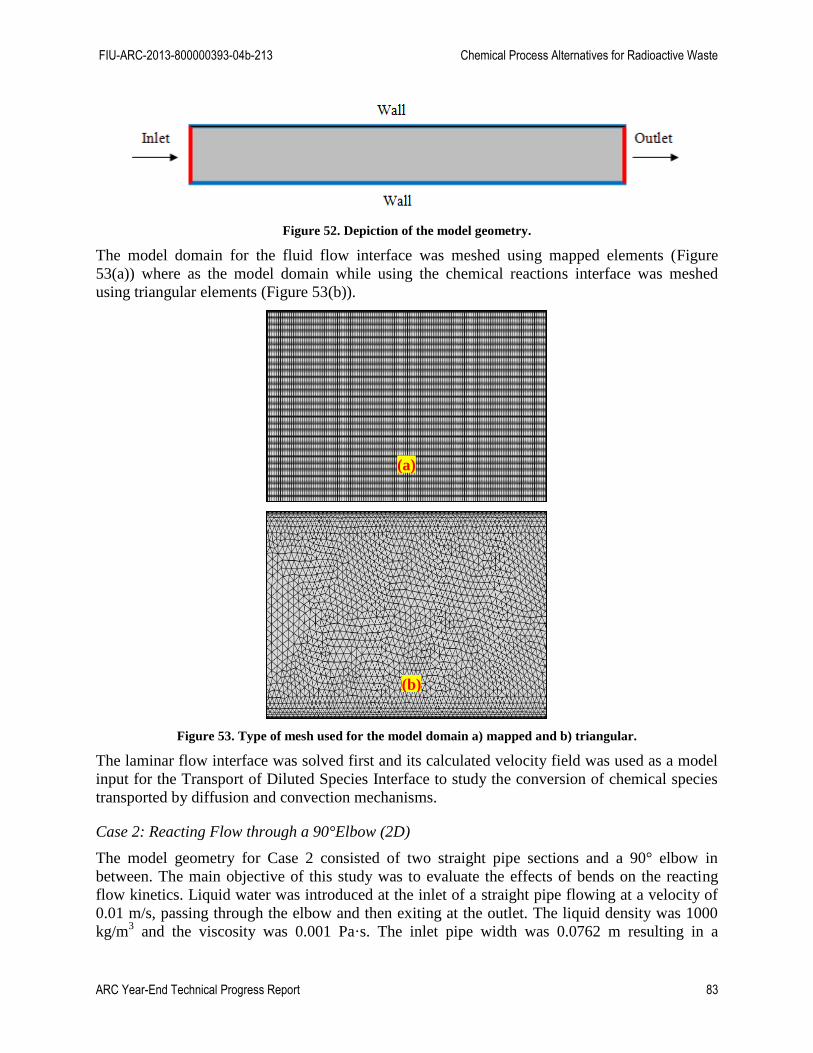
FIU-ARC-2013-800000393-04b-213 Chemical Process Alternatives for Radioactive Waste
ARC Year-End Technical Progress Report 83
Figure 52. Depiction of the model geometry.
The model domain for the fluid flow interface was meshed using mapped elements (Figure
53(a)) where as the model domain while using the chemical reactions interface was meshed
using triangular elements (Figure 53(b)).
Figure 53. Type of mesh used for the model domain a) mapped and b) triangular.
The laminar flow interface was solved first and its calculated velocity field was used as a model
input for the Transport of Diluted Species Interface to study the conversion of chemical species
transported by diffusion and convection mechanisms.
Case 2: Reacting Flow through a 90°Elbow (2D)
The model geometry for Case 2 consisted of two straight pipe sections and a 90° elbow in
between. The main objective of this study was to evaluate the effects of bends on the reacting
flow kinetics. Liquid water was introduced at the inlet of a straight pipe flowing at a velocity of
0.01 m/s, passing through the elbow and then exiting at the outlet. The liquid density was 1000
kg/m3 and the viscosity was 0.001 Pa·s. The inlet pipe width was 0.0762 m resulting in a
(a)
(b)

FIU-ARC-2013-800000393-04b-213 Chemical Process Alternatives for Radioactive Waste
ARC Year-End Technical Progress Report 84
Reynolds number of 762. The pipe length for the inlet and outlet pipe section was 1.828 m each
(Figure 54). Two dilute species A and B with concentrations of 1 mol/m3 and 0.5 mol/m
3 were
introduced at the pipe inlet. The reaction rate of 0.01 mol/m3·s was specified.
The evolution of
the reactant and product species as they are transported over the model geometry consisting of
two pipe sections and a 90° elbow was investigated.
Figure 54. Model geometry for case 2.
The model domain for both the flow and chemical species interface was partitioned into
triangular shape sub-domains using 5885 elements. Figure 55 shows the zoomed in view of the
meshed elbow. A finer mesh was applied at the walls of the pipe than for the rest of the domain.
Figure 55. Meshed geometry for case 2.
Case 3: Reacting Flow through a 90°Elbow (3D)
The case 3 consisted of expanding the previous 2D model into a 3D analysis with the aim of
getting a more accurate representation of the reacting flow kinetics. The model geometry
consisted of two pipe sections and a 90° elbow in between. The pipe diameter was 0.0762 m and
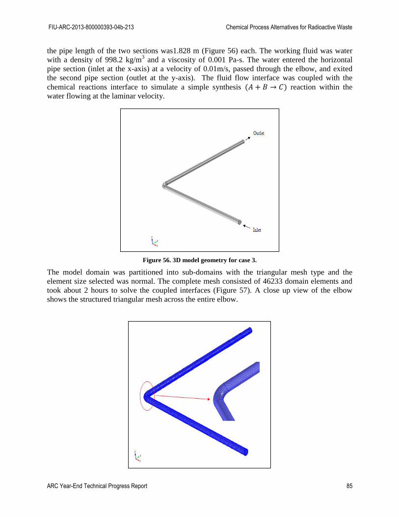
FIU-ARC-2013-800000393-04b-213 Chemical Process Alternatives for Radioactive Waste
ARC Year-End Technical Progress Report 85
the pipe length of the two sections was1.828 m (Figure 56) each. The working fluid was water
with a density of 998.2 kg/m3 and a viscosity of 0.001 Pa-s. The water entered the horizontal
pipe section (inlet at the x-axis) at a velocity of 0.01m/s, passed through the elbow, and exited
the second pipe section (outlet at the y-axis). The fluid flow interface was coupled with the
chemical reactions interface to simulate a simple synthesis reaction within the
water flowing at the laminar velocity.
Figure 56. 3D model geometry for case 3.
The model domain was partitioned into sub-domains with the triangular mesh type and the
element size selected was normal. The complete mesh consisted of 46233 domain elements and
took about 2 hours to solve the coupled interfaces (Figure 57). A close up view of the elbow
shows the structured triangular mesh across the entire elbow.

FIU-ARC-2013-800000393-04b-213 Chemical Process Alternatives for Radioactive Waste
ARC Year-End Technical Progress Report 86
Figure 57. Mesh for the 3D model built for case 3.
Multi-Phase Simulations
The multi-phase simulations focused on modeling the two-phase flow of mixtures in a pipe with
a laminar velocity. The two phases consisted of a solid phase (dispersed) and a liquid phase
(continuous). A mixture interface based on the Euler-Euler approach was used to solve the multi-
phase model. The dispersed phase volume fraction and the continuous phase volume fraction
were computed at the end of the simulations.
The two phase flow at laminar velocity was modeled using the mixture model laminar interface.
The mixture consisted of 10% volume fraction of clay dispersed in water (Figure 58). The
mixture was introduced at the inlet of a horizontal pipe section flowing at a velocity of 0.01 m/s.
The pipe diameter was 0.0762 m and the pipe length was 1.828 m. Water was selected as the
continuous phase and the solids as the dispersed phase. The density of water used was 1000
kg/m3 and a viscosity of 0.001 Pa·s. The density of clay used was 1500 kg/m
3 and the particle
size of 0.001 m.
Figure 58. Model geometry of the multi-phase model.
Governing Equations
The equations governing the mixture model are the momentum and continuity equations and a
volume fraction solution for each phase analyzed. Assumptions made in the simulations include
constant density for each phase, constant pressure field and the velocity between the two phases
can be ascertained from a balance of pressure, gravity, and viscous drag.
The momentum equation for the mixture is given by
[ (
) (
)] (80)
where, u denotes mixture velocity (m/s), ρ is the mixture density (kg/m3), p is the pressure (Pa),
is the mass fraction of the dispersed phase (kg/kg), is the relative velocity between the
two phases (m/s), is the sum of viscous and turbulent stress (kg/(m·s2)), g is the gravity
vector (m/s2), and F is the additional volume forces (N/m
3).
The mixture velocity u is defined as
(81)
Here, c and d denote the volume fractions of the continuous phase and the dispersed phase
(m3/m
3), respectively, the continuous phase velocity (m/s), the dispersed phase velocity

FIU-ARC-2013-800000393-04b-213 Chemical Process Alternatives for Radioactive Waste
ARC Year-End Technical Progress Report 87
(m/s), the continuous phase density (kg/m3), the dispersed phase density (kg/m
3), and ρ
the mixture density (kg/m3).
The mixture density ρ is given by
(82)
where and (kg/m3) are the densities of each of the two phases.
The mass fraction of the dispersed phase is given by
(83)
The relative velocity between two phases is defined by
(84)
Here, (m/s) denotes the relative velocity between the two phases, is a turbulent
dispersion coefficient (m2/s) accounting for extra diffusion due to turbulent eddies. In this case
is set to zero as no turbulent model was used.
The sum of viscous and turbulent stress is
[ ] (85)
where, μ (Pa·s) is the mixture viscosity and (Pa·s) the turbulent viscosity.
The transport equation for Φd, the dispersed phase volume fraction, is
(86)
where, (kg/(m3·s)) is the mass transfer rate from dispersed to continuous phase and (m/s)
is the dispersed phase velocity.
With a constant density for the dispersed phase, the equation becomes
ρ (87)
The continuous phase volume fraction is
(88)
The continuity equation for the mixture is
ρ ρ (89)
The Mixture Model interfaces assumes that the densities of each phase, and ,are constant,
and therefore uses the following alternative form of the continuity equation of the mixture
[
] (90)
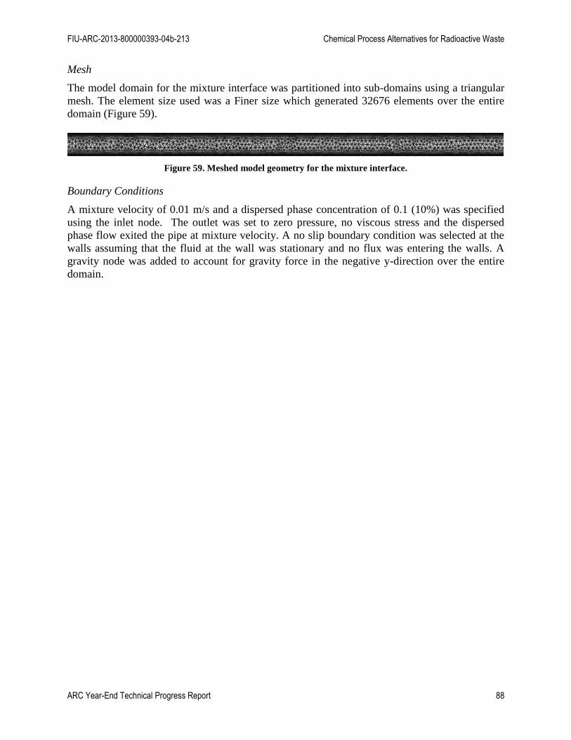
FIU-ARC-2013-800000393-04b-213 Chemical Process Alternatives for Radioactive Waste
ARC Year-End Technical Progress Report 88
Mesh
The model domain for the mixture interface was partitioned into sub-domains using a triangular
mesh. The element size used was a Finer size which generated 32676 elements over the entire
domain (Figure 59).
Figure 59. Meshed model geometry for the mixture interface.
Boundary Conditions
A mixture velocity of 0.01 m/s and a dispersed phase concentration of 0.1 (10%) was specified
using the inlet node. The outlet was set to zero pressure, no viscous stress and the dispersed
phase flow exited the pipe at mixture velocity. A no slip boundary condition was selected at the
walls assuming that the fluid at the wall was stationary and no flux was entering the walls. A
gravity node was added to account for gravity force in the negative y-direction over the entire
domain.
FIU-ARC-2013-800000393-04b-213 Chemical Process Alternatives for Radioactive Waste
ARC Year-End Technical Progress Report 89
RESULTS & DISCUSSION
Single Phase Modeling Simulations
Case 1: Reacting Flow through a Straight Pipe Section (2D)
Mesh Optimization
A mesh optimization study was carried out solely for the laminar flow interface to determine the
optimal mesh that gave the best velocity profile with the least computing time. Four mesh sizes
were simulated for this study: Extremely coarse, coarse, fine and extra fine. The mesh
optimization study parameters are listed in Table 2.
Table 2. Mesh Optimization Study Parameters for Laminar Flow Interface Simulations
Mesh Size No. of Domain
Elements
Solution Time
(s)
Extremely Coarse 3380 8
Coarse 17584 25
Fine 50812 67
Extra Fine 272390 854
The extremely coarse mesh took approximately 8 seconds to solve the model; however, the
velocity profile computed was not smooth. The coarse mesh took 3 times longer to solve the
flow physics but some unevenness in the velocity profile was still apparent as seen in Figure 60.
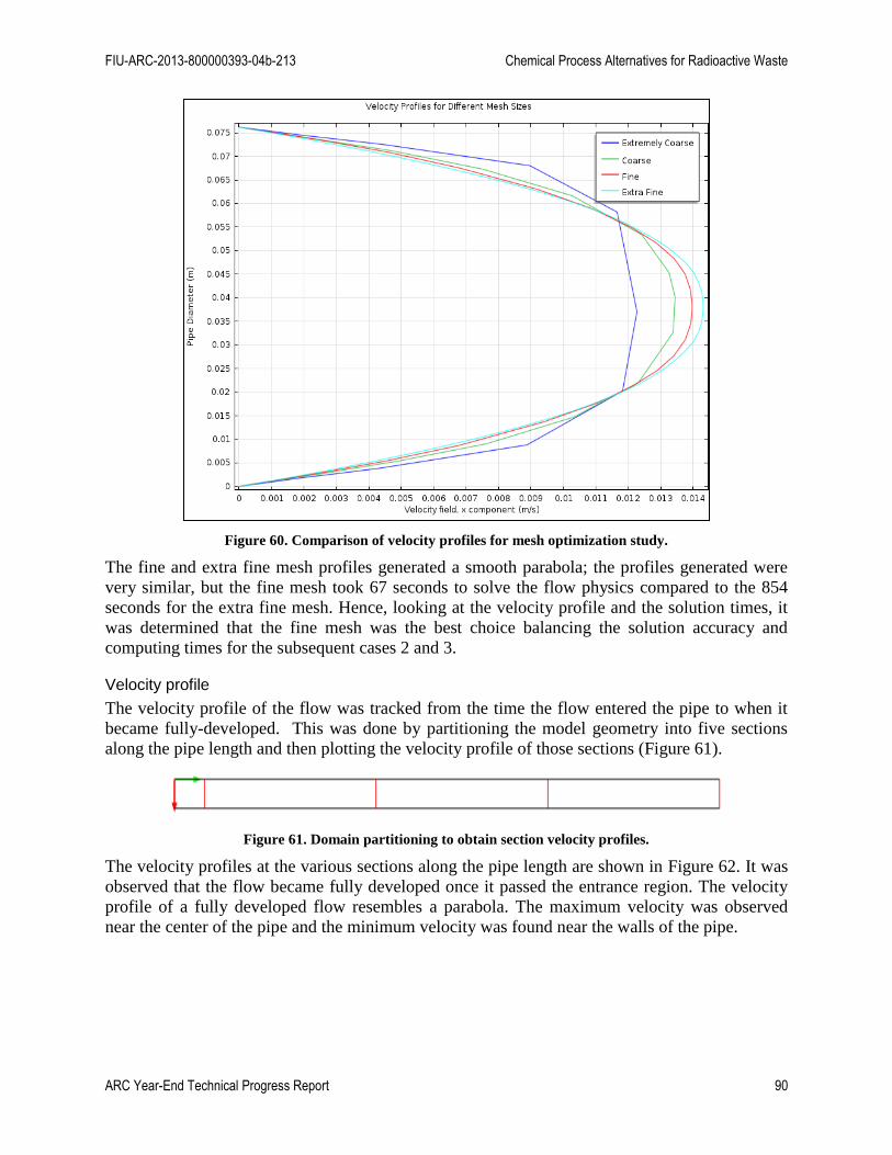
FIU-ARC-2013-800000393-04b-213 Chemical Process Alternatives for Radioactive Waste
ARC Year-End Technical Progress Report 90
Figure 60. Comparison of velocity profiles for mesh optimization study.
The fine and extra fine mesh profiles generated a smooth parabola; the profiles generated were
very similar, but the fine mesh took 67 seconds to solve the flow physics compared to the 854
seconds for the extra fine mesh. Hence, looking at the velocity profile and the solution times, it
was determined that the fine mesh was the best choice balancing the solution accuracy and
computing times for the subsequent cases 2 and 3.
Velocity profile
The velocity profile of the flow was tracked from the time the flow entered the pipe to when it
became fully-developed. This was done by partitioning the model geometry into five sections
along the pipe length and then plotting the velocity profile of those sections (Figure 61).
Figure 61. Domain partitioning to obtain section velocity profiles.
The velocity profiles at the various sections along the pipe length are shown in Figure 62. It was
observed that the flow became fully developed once it passed the entrance region. The velocity
profile of a fully developed flow resembles a parabola. The maximum velocity was observed
near the center of the pipe and the minimum velocity was found near the walls of the pipe.

FIU-ARC-2013-800000393-04b-213 Chemical Process Alternatives for Radioactive Waste
ARC Year-End Technical Progress Report 91
Figure 62. Velocity profiles at different sections of the pipe.
The red color in Figure 63 represents the zone where the maximum velocity was observed and
the blue color represents the area of low velocity. The black arrows are the velocity vectors and
reflected the changes in the velocity profile shape from the inlet to the outlet of the pipe. Initially
the profile was rectangular (as seen near the inlet section of the pipe) and as the flow transitioned
to fully developed, the profile became parabolic.

FIU-ARC-2013-800000393-04b-213 Chemical Process Alternatives for Radioactive Waste
ARC Year-End Technical Progress Report 92
Figure 63. Velocity vectors profiling the shape of the flow along the pipe length.
The laminar flow was characterized by straight streamlines as seen in Figure 64. The fluid
flowed very smoothly in the pipe in an organized fashion and no intermixing of the velocity
streams was observed. The plotted streamlines were color coded with higher velocity represented
by the color red and the lower velocity represented by color blue.
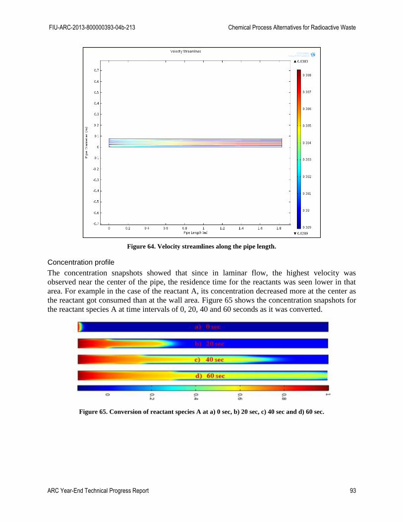
FIU-ARC-2013-800000393-04b-213 Chemical Process Alternatives for Radioactive Waste
ARC Year-End Technical Progress Report 93
Figure 64. Velocity streamlines along the pipe length.
Concentration profile
The concentration snapshots showed that since in laminar flow, the highest velocity was
observed near the center of the pipe, the residence time for the reactants was seen lower in that
area. For example in the case of the reactant A, its concentration decreased more at the center as
the reactant got consumed than at the wall area. Figure 65 shows the concentration snapshots for
the reactant species A at time intervals of 0, 20, 40 and 60 seconds as it was converted.
Figure 65. Conversion of reactant species A at a) 0 sec, b) 20 sec, c) 40 sec and d) 60 sec.
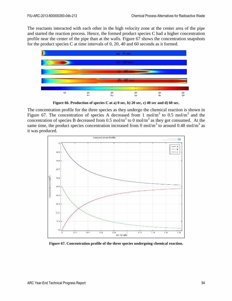
FIU-ARC-2013-800000393-04b-213 Chemical Process Alternatives for Radioactive Waste
ARC Year-End Technical Progress Report 94
The reactants interacted with each other in the high velocity zone at the center area of the pipe
and started the reaction process. Hence, the formed product species C had a higher concentration
profile near the center of the pipe than at the walls. Figure 67 shows the concentration snapshots
for the product species C at time intervals of 0, 20, 40 and 60 seconds as it formed.
Figure 66. Production of species C at a) 0 sec, b) 20 sec, c) 40 sec and d) 60 sec.
The concentration profile for the three species as they undergo the chemical reaction is shown in
Figure 67. The concentration of species A decreased from 1 mol/m3 to 0.5 mol/m
3 and the
concentration of species B decreased from 0.5 mol/m3 to 0 mol/m
3 as they got consumed. At the
same time, the product species concentration increased from 0 mol/m3 to around 0.48 mol/m
3 as
it was produced.
Figure 67. Concentration profile of the three species undergoing chemical reaction.
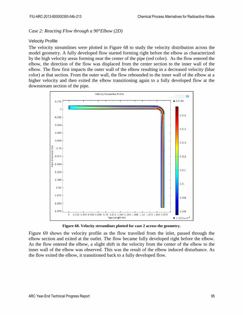
FIU-ARC-2013-800000393-04b-213 Chemical Process Alternatives for Radioactive Waste
ARC Year-End Technical Progress Report 95
Case 2: Reacting Flow through a 90°Elbow (2D)
Velocity Profile
The velocity streamlines were plotted in Figure 68 to study the velocity distribution across the
model geometry. A fully developed flow started forming right before the elbow as characterized
by the high velocity areas forming near the center of the pipe (red color). As the flow entered the
elbow, the direction of the flow was displaced from the center section to the inner wall of the
elbow. The flow first impacts the outer wall of the elbow resulting in a decreased velocity (blue
color) at that section. From the outer wall, the flow rebounded to the inner wall of the elbow at a
higher velocity and then exited the elbow transitioning again to a fully developed flow at the
downstream section of the pipe.
Figure 68. Velocity streamlines plotted for case 2 across the geometry.
Figure 69 shows the velocity profile as the flow travelled from the inlet, passed through the
elbow section and exited at the outlet. The flow became fully developed right before the elbow.
As the flow entered the elbow, a slight shift in the velocity from the center of the elbow to the
inner wall of the elbow was observed. This was the result of the elbow induced disturbance. As
the flow exited the elbow, it transitioned back to a fully developed flow.

FIU-ARC-2013-800000393-04b-213 Chemical Process Alternatives for Radioactive Waste
ARC Year-End Technical Progress Report 96
Figure 69. Velocity profiles plot as the flow travels through the inlet, elbow and outlet (x-axis is the velocity
(m/s) and y-axis is the pipe diameter (m)).
Concentration Profile
The transition of the species from the reactants to a product as they underwent a chemical
reaction is shown in Figure 70. The concentration of product species was found to be the highest
at the inner wall of the elbow and near the center of the pipe as the flow moved towards the
outlet. This was due to the higher velocity observed in those areas. The residence time of the
reactants was lower at the higher velocity areas resulting in the production of species C in those
sections. This was characterized by an increased concentration of product species C (red color)
observed at the inner wall of the elbow and thereafter. Figure 70 shows the concentration
snapshots of the product species C being formed at time intervals of 0, 60, 120, 200, 300 and 400
seconds, respectively.
Figure 70. Concentration snapshots of species C at a) 0 sec, b) 60 sec, c) 120 sec, d) 200 sec, e) 300 sec and f)
400 sec.
Inlet Elbow Outlet

FIU-ARC-2013-800000393-04b-213 Chemical Process Alternatives for Radioactive Waste
ARC Year-End Technical Progress Report 97
Case 3: Reacting Flow through a 90°Elbow (3D)
Velocity Profile
As the fluid travelled through the pipe and entered the elbow entrance, the high velocity
streamlines deviated from the center of the pipe to the inner wall due to the elbow induced flow
disturbance. A maximum velocity of 0.016 m/s was observed at the inner elbow wall (red
streamlines). The flow exited the elbow impacting the outer pipe wall at a higher velocity than at
the center of the pipe and eventually the flow transitioned into a fully developed flow as it
travelled towards the outlet (Figure 71).
Figure 71. Velocity streamlines for the 3D laminar flow model.
The 2D model showed a maximum velocity of 0.0156 m/s (Figure 68) compared to the 0.016 m/s
(Figure 71) computed by the 3D model. Hence it was concluded that the 2D model was
sufficient to get an accurate representation of the laminar reacting flow kinetics and a 3D
analysis was not needed.
Concentration Profile
The evolution of the species during the reaction process was studied from the concentration
surface profile. The reactant species A and B were introduced at the pipe inlet and transported in
the pipe via convection and diffusion mechanisms. Since the laminar flow is characterized by
the maximum velocity occurring near the center of the pipe, the residence time of the reactants

FIU-ARC-2013-800000393-04b-213 Chemical Process Alternatives for Radioactive Waste
ARC Year-End Technical Progress Report 98
was lower at the center of the pipe. The reaction spurred as they came in contact with one
another resulting in the formation of the product species C. The concentration of species C was
found to be the highest in the areas of higher velocity such as the elbow inner wall and the pipe
outer wall after the reacting flow exited the elbow. The red color represents the maximum
concentration of 0.5 mol/m3 for species C. The concentration snapshots of species C at 0, 100,
200, 300, 400 and 500 sec is shown in Figure 72.
Figure 72. Concentration of species C at a) 0 sec, b) 100 sec, c) 200 sec, d) 300 sec, e) 400 sec and f) 500 sec.
Multi-Phase Simulations
Solids Settling
In Figure 73 the continuous phase (water) is represented by the blue color and the dispersed
phase (clay) is represented by the pink color. As the mixture of solids and liquid was transported
along the pipe length, the heavier solids started to settle at the bottom of the pipe and resulted
into a gradual formation of a bed of solids. Figure 73 shows the surface dispersed volume
fractions at 0, 10, 20, 30, 60, 80 and 90 seconds, respectively.
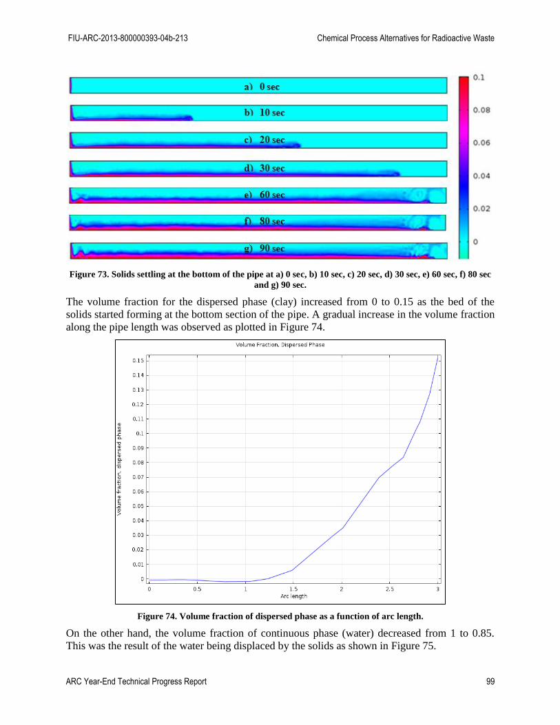
FIU-ARC-2013-800000393-04b-213 Chemical Process Alternatives for Radioactive Waste
ARC Year-End Technical Progress Report 99
Figure 73. Solids settling at the bottom of the pipe at a) 0 sec, b) 10 sec, c) 20 sec, d) 30 sec, e) 60 sec, f) 80 sec
and g) 90 sec.
The volume fraction for the dispersed phase (clay) increased from 0 to 0.15 as the bed of the
solids started forming at the bottom section of the pipe. A gradual increase in the volume fraction
along the pipe length was observed as plotted in Figure 74.
Figure 74. Volume fraction of dispersed phase as a function of arc length.
On the other hand, the volume fraction of continuous phase (water) decreased from 1 to 0.85.
This was the result of the water being displaced by the solids as shown in Figure 75.

FIU-ARC-2013-800000393-04b-213 Chemical Process Alternatives for Radioactive Waste
ARC Year-End Technical Progress Report 100
Figure 75. Volume fraction of continuous phase as a function of arc length.

FIU-ARC-2013-800000393-04b-213 Chemical Process Alternatives for Radioactive Waste
ARC Year-End Technical Progress Report 101
CONCLUSIONS
The overall project conclusion was that Comsol Multiphysics 4.3bTM
could efficiently model the
reacting flow kinetics. The analysis of reacting flow kinetics included understanding how the
flow field affected the chemical reaction process. For the single phase models, the maximum
velocity was observed near the center of the pipe and the minimum velocity at the walls of the
pipe as the fluid transitioned into a fully developed flow. The addition of an elbow displaced the
higher velocity fluid from the center section to the inner wall of the elbow. Hence, the residence
time of the reactants was found to be lower at the center of the pipe and at the inner elbow (high
velocity areas) as they got converted into products. This was characterized by an increased
concentration of product species observed in those sections. The comparison of the 2D and 3D
reacting flow analysis for the case where flow was simulated across a 90° elbow showed similar
results. The 2D model showed a maximum velocity of 0.0156 m/s (Figure 68) compared to the
0.016 m/s (Figure 71) computed by the 3D model. The concentration snapshots showed that the
computed maximum concentration of product species was 0.45 mol/m3 for both the 2D and 3D
analysis. Hence, the 2D model was sufficient to get an accurate representation of the laminar
reacting flow kinetics and a 3D study was not needed for other cases.
The mixture model was only simulated for the flow interface. The coupling of the flow interface
to the chemical reactions was not done during this performance period. The mixture simulations
consisted of a two phase flow (10% vol. fraction of solids dispersed in water) across a horizontal
pipe section. Settling of solids was observed near the bottom of the pipe as the mixture flowed
from the inlet to the outlet. The volume fraction of the dispersed phase increased from 0 to 0.15
as the bed of solids started forming. As the water was displaced by the solids, the volume
fraction of the continuous phase decreased from 1 to 0.85.
Future work will include coupling the chemical reaction to the two phase mixture model. The
dynamic processes such as precipitation, particle agglomeration, particle breakup will also be
incorporated. The modeling efforts will be expanded from the current laminar models to the
turbulent models.

FIU-ARC-2013-800000393-04b-213 Chemical Process Alternatives for Radioactive Waste
ARC Year-End Technical Progress Report 102
REFERENCES
1. Lindner, J. S. et al. 2002. Dial/MSU Prevention of Solids Formation FY 2000 Status Report
Part II: Modeling of Slurry Transport and Saltwell Pumping, reported in ORNL/TM-
2000/302, Mississippi State University, Starkville, Mississippi.
2. Rector, D. R., Stewart, M. L., Poloski, A. P. 2009. Modeling of Sediment Bed Behavior for
Critical Velocity in Horizontal Piping, Pacific Northwest National Laboratory, and Richland,
Washington.
3. McKay, R. L., F. F. Erian, C. J. Call, and E. A. Daymo. 1994. Slurry Transport of Hanford
Tank Wastes: Open Technical Issues and Recommended Actions, Letter Report DSTRTP
CY94-012, Pacific Northwest National Laboratory, Richland, Washington.
4. Washenfelder, D. J. 1978. Occurrence Report: Plugged Cross-Country Transfer Line, OR-78-
88, Rockwell Hanford Operations, Richland, Washington.
5. Reynolds, D. A. 2000. Status of Waste Transfers, Criteria, and Plans presented at the Third
Saltcake Dissolution and Feed Stability Workshop, Richland Washington.
6. Servin, M.A. 2012. Feasibility Study of Pressure Pulsing Pipeline Unplugging Technologies
for Hanford, Washington River Protection Solution, LLC, Richland, Washington.
7. Welch, T.D. 2001. Tank Waste Transport, Pipeline Plugging, and the Prospects for Reducing
the Risk of Waste Transfers, ORNL/TM-2001/157, Oak Ridge National Laboratory,
Tennessee.
8. Hall, M. N. 2007. Design Guide: Avoiding Chemical Line Plugging-Plant Design
Considerations, 24590-WTP-GPG-M-0059, Rev-0, Bechtel National Inc, Richland,
Washington.
9. Herting, D. L. 1980. Evaporator Feeds High in Phosphates, 65453-80-296, Appendix B-
Internal Letters Addressing Phosphate Solubility in RPP-17427, Rockwell Hanford
Operations, Richland, Washington.
10. Herting, D. L. 1987. Phosphate Solubility in Simulated Defense Waste, Appendix B-Internal
Letters Addressing Phosphate Solubility in RPP-17427, Rockwell Hanford Operations,
Richland, Washington.
11. Herting, D. L. 1999. Cooling Test Results, Tank 241-AX-101, Appendix B-Internal Letters
Addressing Phosphate Solubility in RPP-17427, Rockwell Hanford Operations, Richland,
Washington.
12. Barney, G.S., 1976. Vapor-Liquid-Solid Phase Equilibria of Radioactive Sodium Salt Waste
at Hanford, ARH-ST-133, Atlantic Richfield Hanford Company, Richland, Washington.
13. Bunker, B. C. et al. 1995a. Colloidal Studies for Solid/Liquid Separation Studies in Tank
Waste Treatment Science: Report for the First Quarter FY 1995, J.P. LaFemina, ed. PNL-
10762, Pacific Northwest Laboratory, Richland, Washington.
14. Liu, J., L.R. Pederson, and L. Q. Wang. 1995b. Solid-Phase Characterization in Flammable-
Gas-Tank Sludges by Electron Microscopy, PNL-10723, Pacific Northwest Laboratory,
Richland, Washington.
15. Liu, J., L.E. Thomas, Y.L. Chen, and L.Q. Wang. 1995a. Sludge Characterization Studies in
Tank Waste Treatment Science: Report for the Second Quarter FY 1995a, J.P. LaFemina, ed,
PNL-10763, Pacific Northwest Laboratory, Richland, Washington.
16. Knight, M. A., Conner, J. M., Templeton, J. W. 2003. Dilution and Flushing Requirements
to Avoid Solids Precipitation and Deposition during Tank Waste Transfers, RPP-17427,
CH2M Hill Hanford Group, Richland, Washington.

FIU-ARC-2013-800000393-04b-213 Chemical Process Alternatives for Radioactive Waste
ARC Year-End Technical Progress Report 103
17. Welch, T.D. 2002. Tank Waste Transport Stability: Summaries of Hanford Slurry and Salt
Solutions Studies for FY 2000, ORNL/TM-2000/302, Oak Ridge National Laboratory,
Tennessee.
18. Shekarriz, A., Y. Onichi, P. A. Smith, M. Sterner, D. R. Rector, and J. Virden. 1997. Cross-
Site Transfer System at Hanford: Long-Term Strategy for Waste Acceptance, PNNL-11497,
Pacific Northwest National Laboratory, Richland, Washington.
19. Cragnilino, A.G. et al. 1997. Hanford Tank Waste Remediation System Familiarization
Report, CNWRA 97-001, Center for Nuclear Waste Regulatory Analyses San Antonio,
Texas.
20. Julyk, L. J., T. C. Oten, and W. L. Willis. 2002. Waste Feed Delivery Transfer Analysis,
RPP-5346, CH2M Hill Hanford Group, Inc., Richland, Washington.
21. Buchanan, J. R. 2004. Temporary Waste Transfer Line Management Program Plan, CH2M
Hill Hanford Group, Richland, Washington.
22. Broz, R. E. 1994. Tank Farm Hazards Assessment, WHC-SD-PRP-HA-013, Rev-0, Hanford.
23. Coles, G.A. 1995. Risk and Reliability Information about the Cross-Site Transfer System,
WHC Internal Memo #GAC-8M400-95-002, Westinghouse Hanford Company, Richland,
Washington.
24. Brantley, W.M. 1996. Functional Design Criteria for Project W-058, Replacement of the
Cross-Site Transfer System, WHC-SD-W058-FDC-001, Rev-4. Westinghouse Company,
Richland, Washington.
25. MacLean, G. T. et al. 2003. Use of Environmental Simulation Program (ESP) to Simulate
Complex Waste Treatment Processes, Waste Management Conference, Fluor Federal
Services, Richland, Washington.
26. Lidell KC and DF Burnett. 2000. Critical Transport Velocity: A Review of Correlations and
Models. RPP-7185, Rev-0, CH2M Hill Hanford Group, Richland, Washington.
27. Jewett JR, DA Reynolds, SD Estey, L Jensen, NW Kirch, and Y Onishi. 2002. Values of
Particle Size, Particle Density, and Slurry Viscosity to Use in Waste Feed Delivery Transfer
System Analysis, RPP- 9805, Rev-1, Numatech Hanford Corporation, CH2M HILL Hanford
Group, Inc., Richland, Washington.
28. Oroskar AR and RM Turian. 1980. The Critical Velocity in Pipeline Flow of Slurries,
AICHE Journal 26(4), 550-558.
29. Gillies, RG and CA Shook. 1991. A Deposition Velocity Correlation for Water Slurries,
Canadian Journal of Chemical Engineering, 69(5), 1225-1228.
30. Estey, S. D., and T. A. Hu. 1998. Flow Velocity Analysis for Avoidance of Solids Deposition
During Transport of Hanford Tank Waste Slurries, HNF-2728, Lockheed Martin Hanford
Corporation, Richland, Washington.
31. Hall, M. N. 2007. Design Guide: Avoiding Chemical Line Plugging-Plant Design
Considerations, 24590-WTP-GPG-M-0059, Rev-0, Bechtel National Inc, Richland,
Washington.
32. Poloski, A. P. et al., 2009. Deposition Velocities of Newtonian and Non-Newtonian Slurries
in Pipelines, PNNL-17639, WTP-RPT-175, Rev-0, Pacific Northwest National Laboratory,
Richland, Washington.
33. Ebadian, M., C. Lin, and J. L. Xu. 1999. Plugging and Unplugging of Waste Transfer
Pipelines, Preliminary Data and Results, FY 1998 Year End Report, Florida International
University (FIU), Center for Engineering and Applied Sciences, Miami, Florida.

FIU-ARC-2013-800000393-04b-213 Chemical Process Alternatives for Radioactive Waste
ARC Year-End Technical Progress Report 104
APPENDIX A
ITS Final Test Report submitted to FIU

www.itoms.com
1 of 48
Feasibility: Ultrasonic Spectroscopy Characterisation of HLW Stimulant
Richard Tweedie, Wioletta Jablonska
October 2012
Customer: Florida International University
Summary
Leading on from a feasibility study on ultrasound spectroscopy for the characterisation of a HLW stimulant at FIU in
Miami, ITS agreed to repeat the experiments to further understand the practicality of the method and resolve
measurement and analysis issues which were encountered.
The ITS experiments showed that ultrasound spectroscopy, in the through transmission mode, was superior to the
pulse echo measurements for any given transducer configuration.
The reflection measurements were proposed as a means of monitoring the density of the solution. However, the data
showed significant variability which was traced to two causes; the loss of the reflection signal in the stray echoes and
the ill posed nature for the calculation of reflection co-efficient, which lead to a sensitivity to noise. Increasing the size
of the transducers reduced the noise and improved the result but using 25mm transducers compared to 10mm
devices did not eliminate the problem.
Closer examination showed that the density value results were largely dependent on the speed of sound rather than
the reflection co-efficient, which was dominated by the mismatch between the delay line material and the sample.
Hence the reflection method offers little advantage over the use of the speed of sound.
The effect of different materials at different concentrations, and different mixtures of materials, was examined to
determine the effectiveness of the speed of sound measurement for this application. The modelling and the
measurements both showed that the aluminium hydroxide acoustic velocity increased with concentration, while the
zirconium dioxide and stainless steel acoustic velocities decreased with concentration. Measurements using mixed
samples showed that this resulted in the acoustic velocities of the three samples effectively cancelling each other out
with the combined acoustic velocity being less dependent on concentration.
Future work should concentrate on obtaining high quality attenuation data and velocity data using through
transmission measurements and a specialist high concentration measurement system, to enable measurements at
the concentrations encountered in the HLW tanks at Hanford.

www.itoms.com October 2012
2 of 48
1. Table of Contents
Feasibility: Ultrasonic Spectroscopy Characterisation of HLW Stimulant ........................................................................ 1
Summary ........................................................................................................................................................................... 1
1. Table of Contents ...................................................................................................................................................... 2
2. List of Figures ............................................................................................................................................................. 5
3. List of Tables .............................................................................................................................................................. 7
4. Introduction ............................................................................................................................................................... 8
5. Ultrasound Spectroscopy .......................................................................................................................................... 8
5.1. Ultrasound particle sizing ................................................................................................................................... 9
5.2. Ultrasound rheology ......................................................................................................................................... 10
6. The U2s USS system ................................................................................................................................................. 11
6.1. Reflection measurements................................................................................................................................. 12
7. Modelling of Stimulant ............................................................................................................................................ 13
7.1. Distribution of each discrete phase .............................................................................................................. 14
7.2. Modelling results .............................................................................................................................................. 16
7.2.1. Individual materials ....................................................................................................................................... 16
7.2.2. Total sample attenuation .......................................................................................................................... 17
7.2.3. Total sample velocity ................................................................................................................................. 18
7.2.4. Comparison with actual ............................................................................................................................. 18
7.2.5. Effectiveness of high concentrations......................................................................................................... 18
7.3. Simulated concentration ladders. .................................................................................................................... 19
7.3.1. Simulated aluminium hydroxide concentration ladder ............................................................................. 19
7.3.2. Simulated zirconium dioxide concentration ladder .................................................................................. 20
7.3.3. Simulated stainless steel concentration ladder......................................................................................... 21
8. Experimental programme ........................................................................................................................................ 23
8.1. Experimental plan ............................................................................................................................................. 23

www.itoms.com October 2012
3 of 48
8.2. Experimental method ....................................................................................................................................... 23
8.3. The preparation of the solutions ...................................................................................................................... 24
8.4. Methodology .................................................................................................................................................... 24
9. Results ..................................................................................................................................................................... 25
9.1. Sodium nitrate solution .................................................................................................................................... 25
9.2. Solid suspensions .............................................................................................................................................. 26
9.2.1. Suspension of aluminium hydroxide Al(OH)3 in water ............................................................................. 26
9.2.2. Suspension of zirconium oxide ZrO2 in water ............................................................................................ 27
9.2.3. Repeatability of the measurements .......................................................................................................... 28
9.2.4. Suspension of stainless steel (SS316) in water. ......................................................................................... 30
9.2.5. Suspension of aluminum hydroxide in NaNO3aq solution ........................................................................ 31
9.2.6. Complex powder mixtures in NaNO3 aqueous solution ........................................................................... 33
9.3. Density measurement ...................................................................................................................................... 35
9.3.1. Density of Na(NO)3 solution ...................................................................................................................... 35
9.3.2. Density of aluminium hydroxide suspension in Na(NO)3) ........................................................................ 37
9.3.3. Density of aluminium hydroxide suspension in water .............................................................................. 38
9.3.4. Density of complex mixture in Na(NO)3 .................................................................................................... 39
9.4. Review of Original Data .................................................................................................................................... 39
10. Discussion .............................................................................................................................................................. 40
10.1. Ultrasonic Velocity of constituent materials .............................................................................................. 40
10.2. The reflection coefficient ............................................................................................................................... 40
11. Conclusions ............................................................................................................................................................ 41
12. Recommendations for further work ...................................................................................................................... 42
13. References ............................................................................................................................................................. 42
14. Appendix 1 ............................................................................................................................................................. 43
Table 8 Composition of Sodium Nitrate solution ........................................................................................................ 43

www.itoms.com October 2012
4 of 48
Table 9 Composition of Aluminium Hydroxide Suspensions in water ........................................................................ 44
Table 10 Composition of Zirconium Dioxide suspension ........................................................................................... 45
Table 11 Composition of Stainless Steel suspension .................................................................................................. 46
15. Appendix 2 ............................................................................................................................................................. 48

www.itoms.com October 2012
5 of 48
2. List of Figures
Figure 1: The relationship between particle size and attenuation loss for different frequencies 10
Figure 2: The U2s USS system with sensor used in the experiments 11
Figure 3 Sensor configurations: transmission, probe, and reflectance 11
Figure 4 Reflection mode measurement method 12
Figure 5 Previously published particle size distribution plots for the AY-102 and previous stimulant particle size plots 14
Figure 6 The particle size distributions for each of the constituents of the theoretical stimulant used in this report 14
Figure 7 The overall volume distribution of the theoretical stimulant used in the model experiments for this report 15
Figure 8 Simulated attenuation spectra for the individual constituents of the stimulant material 16
Figure 9 Simulated velocity spectra for the individual constituents of the stimulant material plot 17
Figure 10 The spectra of the total attenuation for the stimulant material based on the values given in Table 1 17
Figure 11 The spectra of the total velocity for the stimulant material based on the values given in Table 1 18
Figure 12 Attenuation values from measurements of sample recovered from the tanks at Hanford 18
Figure 13 A plot of measured attenuation verses concentration for a 300nm silica sample showing the impact
of the non-linear relationship between scattering and concentration at higher concentration levels 19
Figure 14 Attenuation at 9.9MHz verses concentration (below 5%v) for aluminium hydroxide 19
Figure 15 Velocity at 9.9MHz verses concentration (below 5%v) for aluminium hydroxide 20
Figure 16 Attenuation at 9.9MHz verses concentration (below 5%v) for zirconium dioxide 20
Figure17. Velocity at 9.9MHz verses concentration (below 5%v) for zirconium dioxide 21
Figure 18. Attenuation at 9.9MHz verses concentration (below 5%v) for stainless steel 21
Figure.19. Velocity at 9.9MHz verses concentration (below 5%v) for stainless Steel 22
Figure 20.Comparison of ultrasonic velocity values from measurements of NaNO3 aq solutions collected with the
USS instrument in Manchester with the presented data in the Phase1, Hanford project and the data published by
Rohman N., Mahiuddin S. [1]
25 Figure 21 Attenuation values from measurements of NaNO3 aq solutions collected by the USS instrument low
concentration system 25
Figure 22 Ultrasonic velocity values from measurements of Al(OH)3 aq suspensions collected by the USS
instrument low concentration system 26
Figure 23 Attenuation values from measurements of Al(OH)3 aq suspensions collected by the USS instrument
low concentration system 27

www.itoms.com October 2012
6 of 48
Figure 24 Ultrasonic velocity values from measurements of ZrO2 aq suspensions collected by the USS
instrument low concentration system 28
Figure 25. Reproducibility of the ultrasonic measurements of ZrO2 aq suspension collected by the USS
instrument low concentration system 29
Figure 26 Attenuation measurements of ZrO2 aq suspension collected by the USS instrument low concentration system 29 Figure 27 Repeatability of attenuation measurements of ZrO2 aq suspension collected by the USS instrument
low concentration system 30
Figure 28 Velocity measurements of stainless steel aq suspension collected by the USS instrument
low concentration system 30
Figure 29 Attenuation measurements of stainless steel aq suspension collected by the USS instrument
low concentration system 31
Figure.30 Ultrasonic velocity values from measurements of Al(OH)3 in NaNO3 aq suspensions collected by
the USS instrument low concentration system. 31
Figure 31 Attenuation values from measurements of Al(OH)3 in NaNO3 aq suspensions collected by the
USS instrument low concentration system 32
Figure 32 Ultrasonic velocity values from measurements of complex powders mixture in NaNO3 aq
suspensions collected by the USS instrument Hi-C concentration system 33
Figure 33 Attenuation values from measurements of complex powders mixture in NaNO3 aq suspensions
collected by the USS instrument Hi-C concentration system 34
Figure 34 Density values from measurements of NaNO3q solutions collected by the USS instrument
Hi-C concentration system 34
Figure 35 Density values from measurements of aluminium hydroxide in NaNO3q solutions compared to the
calculated value 35
Figure 36 Density values from measurements of aluminium hydroxide in NaNO3q solutions plotted against
the calculated value 36
Figure 37 Density values from measurements of aluminium hydroxide in water plotted against the calculated value 37
Figure 38 Density values from measurements of complex mixtures in NaNO3 aq suspensions plotted against the
calculated value 38
Figure 39 The effect of changing liquid density on the reflection co-efficient and ultrasonic velocity 40

www.itoms.com October 2012
7 of 48
3. List of Tables
Table 1 Size and concentration information from Tank HY-102 used as the basis for the sample constituents
for the modelling exercise 13
Table 2 Physical Properties for the materials used in the simulation 14
Table.3 Attenuation values from measurements of complex powders mixture in NaNO3 aq suspensions,
Collected by the USS instrument Hi-C concentration system 33
Table 4. Attenuation values from measurements of complex powders mixture in NaNO3 aq suspensions,
Collected by the USS instrument Hi-C concentration system 35
Table 5 Comparing Measured Density of sodium Nitrate solution with calculated density 36
Table 6 Comparing Measured Density of Aluminium Hydroxide in water suspension with calculated density. 37
Table.7 Comparing Measured Density of Complex Mixture in Na(NO)3 solution with calculated density. 38
Table 8 Composition of Sodium Nitrate solution 43
Table 9 Composition of Aluminium Hydroxide Suspensions in water 44
Table 10 Composition of Zirconium Dioxide 44
Table 11 Composition of Stainless Steel suspension 45
Table 12 Composition of Suspension of Al(OH)3 in sodium nitrate aqueous solution 46
Table 13 Composition of Complex mixtures 47

www.itoms.com October 2012
8 of 48
4. Introduction
FIU previously rented a U2s low concentration system with a 19mm probe from ITS. The objective was to study the
possible use of the technique for the characterisation of High Level Waste (HLW) slurry from the holding tanks at
Hanford, before or during transfer from the tanks.
The rental results were promising suggesting a possible application in measuring the density using the reflectance
method but the data contained significant artefact. FIU and ITS agreed to collaborate to further study the application
and determine the source of the artefact and verify the results from the original rental.
For further information on the background of the experiments the reader is referred to FY2011 Project #1 Technical
Report ask 15: Advanced HLW Instrumentation Ultrasonic Spectroscopy Phase I Test Summary Report [1]
This report examined two aspects in detail; the attenuation and velocity characteristics were modelled using a first
principles model based on work by Wang and Povey [2] and the measurement of the attenuation, acoustic velocity
and density using the U2s system
The report also reviews the earlier work and determines the reasons for the artefacts but, due to the large amount of
data and limited time, doesn’t not dwell on the detail.
Finally the report discusses the physical mechanisms of the interaction of the measurement with the samples and the
resultant velocity and density data.
5. Ultrasound Spectroscopy
Ultrasonic spectroscopy (USS) is the characterisation of the ultrasonic response of a material to the propagation of a
low level ultrasonic wave. It has a number of inherent and useful features:
• Non-destructive, non-intrusive and inline
• Can be used on opaque samples
• Can be used on both liquids and soft solids
• Simple sample handling with no requirement for manual intervention
• Able to operate over a wide range of frequencies
The ultrasonic spectroscopy data can be used to characterise a range of material or process properties and
behaviours including:
1. Measurement of density and or concentration of discrete phases, mixed liquids or slurries
2. Rheological characterisation of liquids and soft solids through phase velocity
3. Indicative changes in attenuation spectra due to changes in material structure including particle size of colloids in both slurries and emulsions
4. The characterisation of liquids containing bubbles

www.itoms.com October 2012
9 of 48
5.1. Ultrasound particle sizing
Particles absorb and diffract ultrasound energy and hence the change in ultrasound energy of a wave in a slurry or
emulsion is a function of the particle size. Particle size determination from the ultrasonic attenuation spectra is based
on a first principles model.
The attenuation of ultrasound in a dispersed system is caused by a variety of mechanisms (the significance of which
depends on material properties, particle size and sound). These mechanisms include
• Intrinsic losses
• Geometric scattering
• Thermal absorption
• Visco-inertial losses
The ultrasonic absorption is also dependant on the contribution of the continuous phase, which is known as the
intrinsic attenuation. Therefore the addition or excess attenuation coefficient is given as
Scattering: Ultrasonic scattering is the re-direction of acoustic energy away from the incident beam, so it is elastic (no energy is absorbed). The scattering is a function of frequency and particle size and is only significant at very large particle sizes
Thermal losses: Thermal losses are due to temperature gradients generated near the surface of the particle as it is
compressed by the acoustic wave. The resulting thermal waves radiate a short distance into the liquid and into the
particle. Dissipation of acoustic energy caused by thermal losses is the dominant attenuation effect for soft colloidal
particles, including emulsion droplets and latex droplets.
Viscoinertial losses: Viscoinertial losses are due to relative motion between the particles and the surrounding fluid.
The particles oscillate with the acoustic pressure wave, but their inertia retards the phase of this motion. This effect
becomes more pronounced with increasing contrast in density between the particles and the medium. As the liquid
flows around the particle, the hydrodynamic drag introduces a frictional loss. Viscoinertial losses dominate the total
attenuation for small rigid particles, such as oxides, pigments, and ceramics.
All of these mechanisms whatever their source are described by the general term scattering. The model seeks to
account for each of these mechanism scattered sound fields around a single particle. Based on this, the propagation
of sound through the dispersed system can be calculated. By assuming independent scattering it is possible to
separately determine the total attenuation as the sum of the individual mechanisms.
scthvisexc αααα ++≈
intααα −=′cex

www.itoms.com October 2012
10 of 48
Figure 1: The relationship between particle size and attenuation loss for different frequencies. The figure shows the
two major features of the attenuation verses size plot - at small particle sizes the spectra is dominated by differences
in physical properties - the mid range is the visco-inertial region, which is a result of the movement of the particle in a
viscous liquid - while at large particle sizes the attenuation increases rapidly due to geometric scattering.
5.2. Ultrasound rheology
Ultrasound can be used as a measure the rheological properties of a material. Specifically the attenuation and velocity
information can be used to determine the longitudinal bulk modulus of a material.
Where k is the ultrasound wave number ω is the angular velocity ρ and M the longitudinal modulus. * denotes complex
values. The solution of the Navier Stokes equation allows the viscosity to be determined from the attenuation and
velocity values
The advantage in using the ultrasound spectra is the availability of frequency dependant data which provides an indication Newtonian or Non-Newtonian behaviour.
2
3
.2
..3
ω
αρη
c=
ρ
ω *
*
M
k=
Att
en
ua
tio
n

www.itoms.com October 2012
11 of 48
6. The U2s USS system
The U2s ultrasound spectroscopy system is based on the use of transient measurements and is specifically
developed for in-situ or on-line applications. The use of fast transient methods allows data collection in real time
allowing the use of the system on dynamic and rapidly evolving applications, such as crystallization. The Hi–C system
is unique as it uses a novel measurement system which uses digital ultrasound signals to increase the dynamic range
and resolution of the system
The sensor itself is custom designed to match the application. The sensor also does not require the adjustment of
transducer spacing’s during measurement and hence the sensors are robust and process compatible. The sensor
can either be a flow through cell for pipes or a dip in probe for reactors and large vessels.
Figure 2: The U2s USS system with sensor used in the experiments
The U2s can be configured to operate in a number of different methods to best match the application.
1. The probe or pipe method: low concentration liquids and colloids and very fast measurements
2. The coded transmission method: low concentration and high concentration liquids and colloids, moderate
update rate.
3. The reflectance method: developed for extremely highly attenuating materials close to solid.
Figure 3 Sensor configurations: transmission, probe, and reflectance

www.itoms.com October 2012
12 of 48
6.1. Reflection measurements
The reflectance method is based on the contact impedance at the interface between the sensor and sample. Reflectance only measures the material characteristics at the interface but can operate in very highly attenuating materials.
Figure 4 Reflection Mode Measurement Method
The reflectance parameter R can be used to determine the acoustic impedance of the material and hence to calculate the bulk modulus.
** MiXRZ ss ⋅=+= ρ21
21
ZZ
ZZR
+
−=

www.itoms.com October 2012
13 of 48
7. Modelling of Stimulant
The objective of this work was to provide some indication of the expected values for the attenuation and velocity of the
samples and constituent materials, by using the theoretical models of acoustic propagation. The quality of these
models needs to be qualified at the outset. The current state of the art of ultrasonic propagation modelling is limited to
low concentration linear models, by which the attenuation has a linear dependence on concentration. The models do
not account for high concentration crowded particle effects and the impact of non-linear rheology.
The source of information used for the physical properties to input to the models were provided by FIU and also by
using information from papers and the internet. The initial modelling used information previously obtained from studies
of Tank AY-102 to define the particle size and concentration of the samples - as shown in Table 1
Simulant
Material
Specific
Gravity
(S.G.)
Particle
size,
d50
(um)
Volume
%
AY-102 Tank Waste Represented
Gibbsite
(Aluminium
TriHydrate)
2.42 10 52 Represents 53% of waste by
volume
Zirconium Oxide 5.7 12 37 Represents Fe2O3 and MnO2,
which make up 40% of waste by
volume
F120 Silicon
Carbide
3.2 150 6 Ca5OH(PO4)3 makes up 5% solid
by volume
Bismuth Oxide 8.9 38 2 Represents PuO2 (the bounding
material density in the tank)
Stainless Steel
(316)
8 128 3 Represent bounding density and
particle size within tank
Table 1 Size and concentration information from Tank HY-102 used as the basis for the sample constituents for the
modelling exercise
Material Density
(x1000 kg/m3)
Bulk Modulus
(GPa)
Speed of sound
(m/s)
Gibbsite (Aluminium
TriHydrate)
2.42 85 5926
Zirconium Oxide 5.68 91.6 7380
F120 Silicon Carbide 3.2 178 11590
Bismuth Oxide 8.9 7.86 2526
Stainless Steel (316) 7.86 77.2 5790
Table 2 Physical properties for the materials used in the simulation

www.itoms.com October 2012
14 of 48
The previous literature also provided an example of a particle size distribution for the AY 102 tank as shown in Figure
5
Figure 5 Previously published particle size distribution plots for the AY-102 and previous stimulant particle
size plots
It should be noted that the particle size distribution for AY-102 in Figure 5 looks particularly non –physical and the
sampling or PSD method should be questioned. Therefore the modelling of the stimulant was based on the D50 data
given in Table 1 and the assumed distributions are shown for each component of the mixture in Figure 6.
7.1. Distribution of each discrete phase
Figure 6 The particle size distributions for each of the constituents of the theoretical stimulant used in this
report.
The total distribution for the sample is given in Figure 7, note these results are based on a volume distribution.
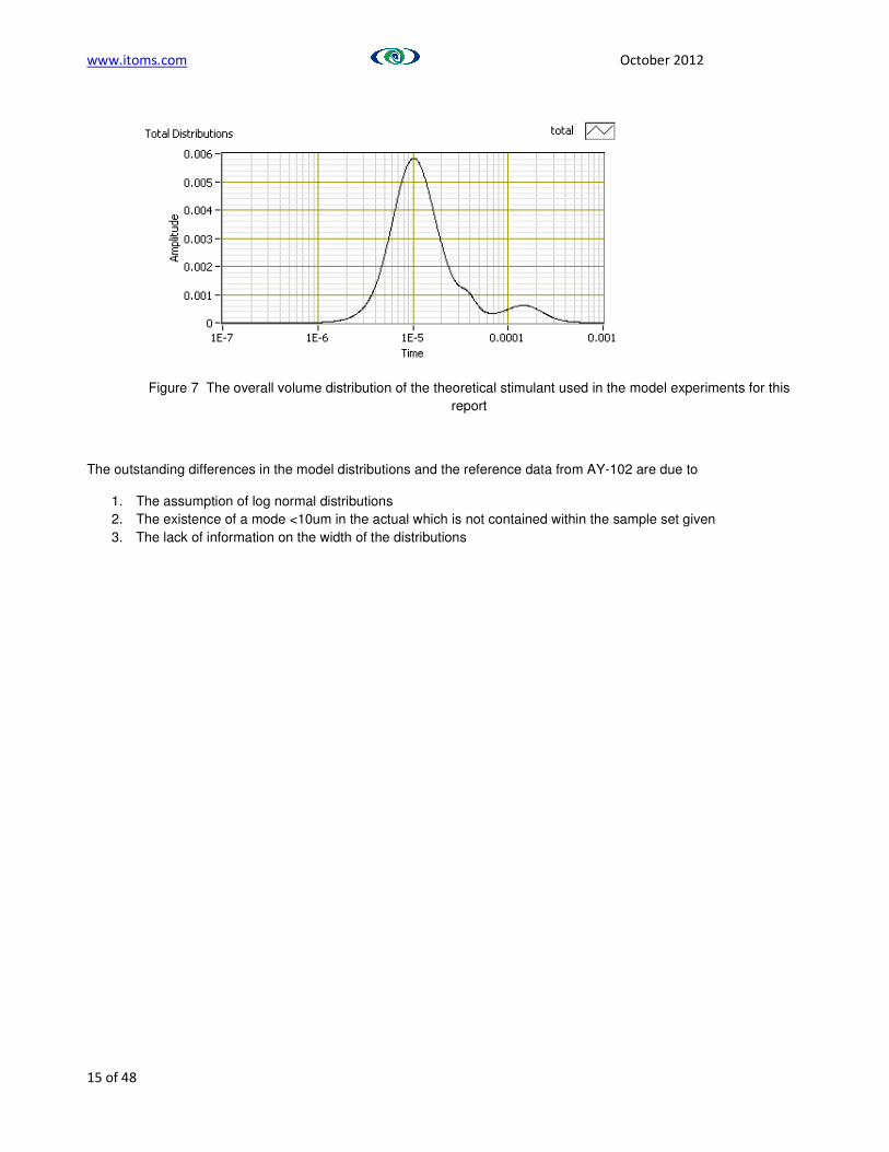
www.itoms.com October 2012
15 of 48
Figure 7 The overall volume distribution of the theoretical stimulant used in the model experiments for this
report
The outstanding differences in the model distributions and the reference data from AY-102 are due to
1. The assumption of log normal distributions
2. The existence of a mode <10um in the actual which is not contained within the sample set given
3. The lack of information on the width of the distributions

www.itoms.com October 2012
16 of 48
7.2. Modelling results
The distributions shown above were used to generate spectra for both attenuation and velocity. To simplify the need
for physical properties the continuous phase was assumed to be water. The model uses has been described by
Wang and Povey and was selected as it included both visco-inertial effects and thermal effects, and is principally
based on an explicit solution to Epstein Carhart, Allegra Hawley (ECAH) for the first two scattering terms A0 and A1.
In the case of velocity, previously published work outlines two cases for the value of the velocity in mixtures of two
components. Urick used a simple volume averaged form of the Wood equation to determine effective compressibility’s
and densities for the overall mixtures.
However, in its original form it is unable to account for the additional effect of scattering due to interfaces within the
sample and particles. Hence a modified version of Urick has been described which has already been discussed in the
previous report [1]. However, this phenomenological model has limited application. By returning to a first principles
scattering model, albeit with a reduced set of scattering terms, we should be able to get a closer agreement for
suspensions.
7.2.1. Individual materials
As can be seen in Figure 8, at the concentrations specified in Table 1 the zirconium dioxide and aluminium hydroxide
attenuations are substantially greater, but, even at very low concentrations, the stainless steel is contributing
significant scattering and hence would be expected to have a substantial effect at higher concentrations.
Figure 8 Simulated attenuation spectra for the individual constituents of the stimulant material
effeff
cρκ .
1=
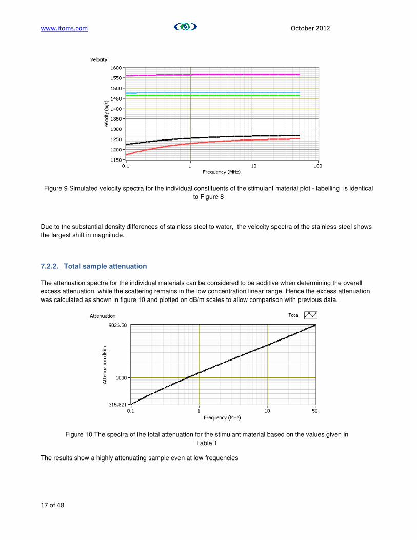
www.itoms.com October 2012
17 of 48
Figure 9 Simulated velocity spectra for the individual constituents of the stimulant material plot - labelling is identical
to Figure 8
Due to the substantial density differences of stainless steel to water, the velocity spectra of the stainless steel shows
the largest shift in magnitude.
7.2.2. Total sample attenuation
The attenuation spectra for the individual materials can be considered to be additive when determining the overall
excess attenuation, while the scattering remains in the low concentration linear range. Hence the excess attenuation
was calculated as shown in figure 10 and plotted on dB/m scales to allow comparison with previous data.
Figure 10 The spectra of the total attenuation for the stimulant material based on the values given in
Table 1
The results show a highly attenuating sample even at low frequencies

www.itoms.com October 2012
18 of 48
7.2.3. Total sample velocity
Figure 11 The spectra of the total velocity for the stimulant material based on the values given in
Table 1
The predicted values of the velocity spectra are surprising low considering the density of the stainless steel and
zirconium dioxide.
7.2.4. Comparison with actual
*drawing is best quality available
Figure 12 Attenuation values from measurements of sample recovered from the tanks at Hanford
The model attenuation is lower than the actual attenuation in the tanks at Hanford this is probably due to the non-
linear effects of the high concentrations of solids in the tanks as described below.
7.2.5. Effectiveness of high concentrations
At high concentrations the material’s attenuation is reduced by particle to particle transmission. This is illustrated
below for 100nm silica from 1-50v%. This is described as multiple scattering by some authors.
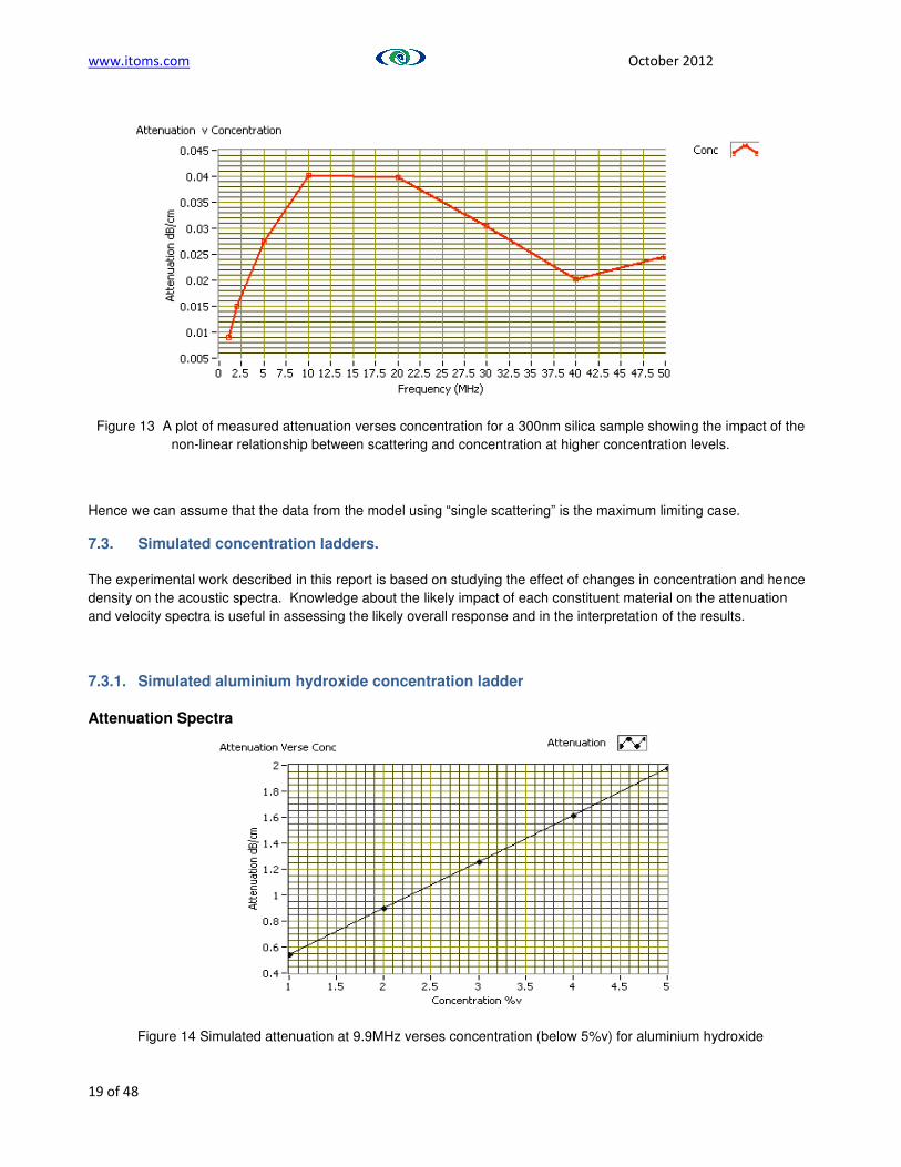
www.itoms.com October 2012
19 of 48
Figure 13 A plot of measured attenuation verses concentration for a 300nm silica sample showing the impact of the
non-linear relationship between scattering and concentration at higher concentration levels.
Hence we can assume that the data from the model using “single scattering” is the maximum limiting case.
7.3. Simulated concentration ladders.
The experimental work described in this report is based on studying the effect of changes in concentration and hence
density on the acoustic spectra. Knowledge about the likely impact of each constituent material on the attenuation
and velocity spectra is useful in assessing the likely overall response and in the interpretation of the results.
7.3.1. Simulated aluminium hydroxide concentration ladder
Attenuation Spectra
Figure 14 Simulated attenuation at 9.9MHz verses concentration (below 5%v) for aluminium hydroxide

www.itoms.com October 2012
20 of 48
Velocity Spectra
Figure 15 Simulated velocity at 9.9MHz verses concentration (below 5%v) for aluminium hydroxide
7.3.2. Simulated zirconium dioxide concentration ladder
Attenuation Spectra
Figure16 Simulated attenuation at 9.9MHz verses concentration (below 5%v) for zirconium dioxide
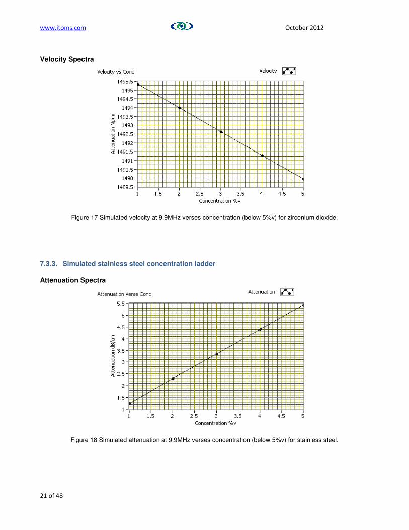
www.itoms.com October 2012
21 of 48
Velocity Spectra
Figure 17 Simulated velocity at 9.9MHz verses concentration (below 5%v) for zirconium dioxide.
7.3.3. Simulated stainless steel concentration ladder
Attenuation Spectra
Figure 18 Simulated attenuation at 9.9MHz verses concentration (below 5%v) for stainless steel.
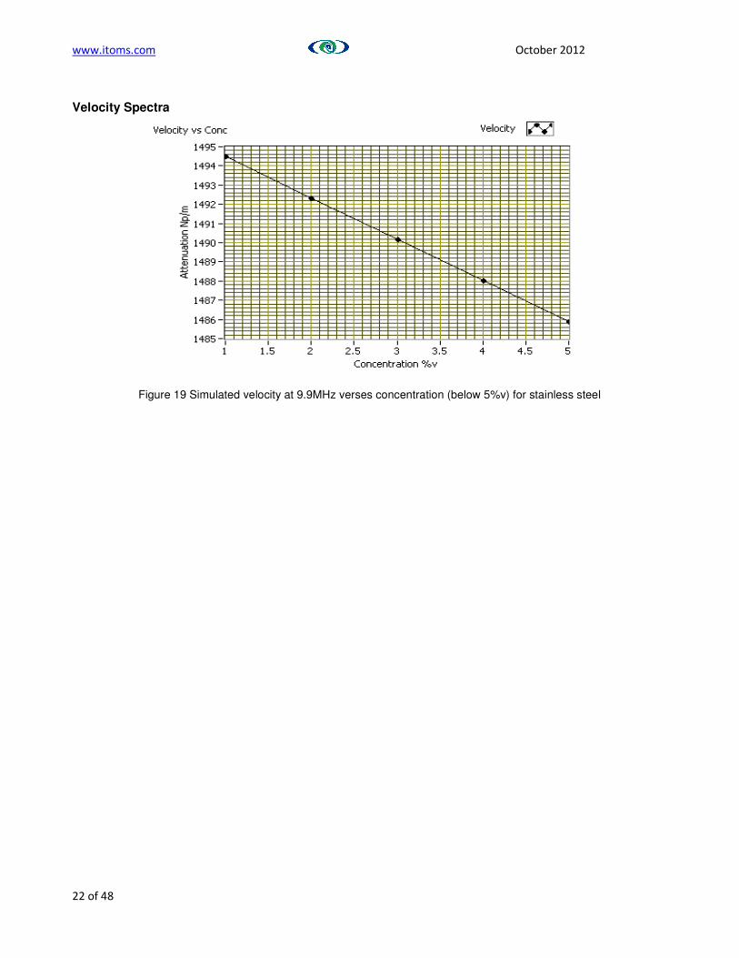
www.itoms.com October 2012
22 of 48
Velocity Spectra
Figure 19 Simulated velocity at 9.9MHz verses concentration (below 5%v) for stainless steel

www.itoms.com October 2012
23 of 48
8. Experimental programme
8.1. Experimental plan
The experimental plan was to measure the ultrasonic characteristics of
• Sodium nitrate aqueous solution
• Aluminium hydroxide in water
• Aluminium hydroxide in sodium nitrate aqueous solution
• Zirconium dioxide in water
• Stainless steel in water
• Complex powder mixtures in sodium nitrate aqueous solution
8.2. Experimental method
Materials:
1) Liquids: i. Distilled water, NaNO3,
2) Solids: i. Aluminium hydroxide Al(OH)3 (S1), ii. Zirconium oxide (ZrO2) (S2) iii. Stainless steel – 316(SS) (S3)
Samples: slurry stimulants, ten repeats of the measurements for every sample.
• All solutions/suspensions were prepared according to proposed concentration ladder 0.1%, 0.5%, 1%,
2%, 3%, 5%, 7%, 10%, 15%, 20%, 25%, (30%, 37.5% for sodium nitrate, precipitation of the solid in
the sample) apart from complex powder mixture samples where the concentration ladder was 1%,
2%, 4%, 6%, 8%, 10%.
• The suspensions were mixed during measurements using a magnetic stirrer.
• The only solutions when the stirrer hasn’t been able to provide the even suspension during the
measurements were the stainless steel ones and so the results from these samples are the most
inconsistent.
Prepared samples:
1) Aqueous solution NaNO3
2) Distilled water + aluminium hydroxide Al(OH)3,
3) Distilled water + zirconium oxide (ZrO2)
4) Distilled water + stainless steel – 316(SS)
5) Solutions of NaNO3* + S1
6) Solutions of NaNO3* + mixtures of solids
*: All Na(NO)3 Solutions were prepared at 13v% and a relative bulk density of 1.17

www.itoms.com October 2012
24 of 48
Parameters of the experiment: room temperature, the volume of the sample 350 ml.
8.3. The preparation of the solutions
An appropriate amount of the substance was dissolved in a medium, the volume of the solution 350ml, using the
measures listed in Appendix 1.
8.4. Methodology
The measurements were carried out using the USS cell in the static and dynamic conditions with a low and Hi-C
(aluminium hydroxide) concentration system. For purpose of the experiments the immersion transducers were used
with no delay line. Every experiment consisted of 10 repeated measurements for each sample. The sample was then
removed from the cell for disposal and new material was added. In the case of sodium nitrate solutions the spacing
between transducers was equal 22 mm, for suspensions it was 10 mm. The system was calibrated using deionised
water as a reference material.
Reflection measurements were carried out using probe in a dynamic condition and Hi-C system. For this experiment
the probe containing transducer with the delay line was used. Ten measurements were collected for every sample.
For all types of tested suspensions the spacing between transducer and reflector was kept as 4 mm. The system was
calibrated using deionised water as a reference material.
Solids Loading Ladder Tests:
ITS performed two sets of solids loading ladder tests on the USS system in a bench-scale setup approved by FIU. The
solids load ladder tests were performed on solutions with a mixture of FIU-provided solids consisting of aluminium
hydroxide, zirconium oxide and stainless steel 316. The mixtures had varying bulk densities in the range of 1.15 to
1.55 g/cc. The solvent was either distilled, RO/DI water, or a sodium nitrate/water solution. Tests were performed on
stirred solution, which provided sufficient mixing power to maintain the solids in suspension. The mixing process is
documented in the test results report.
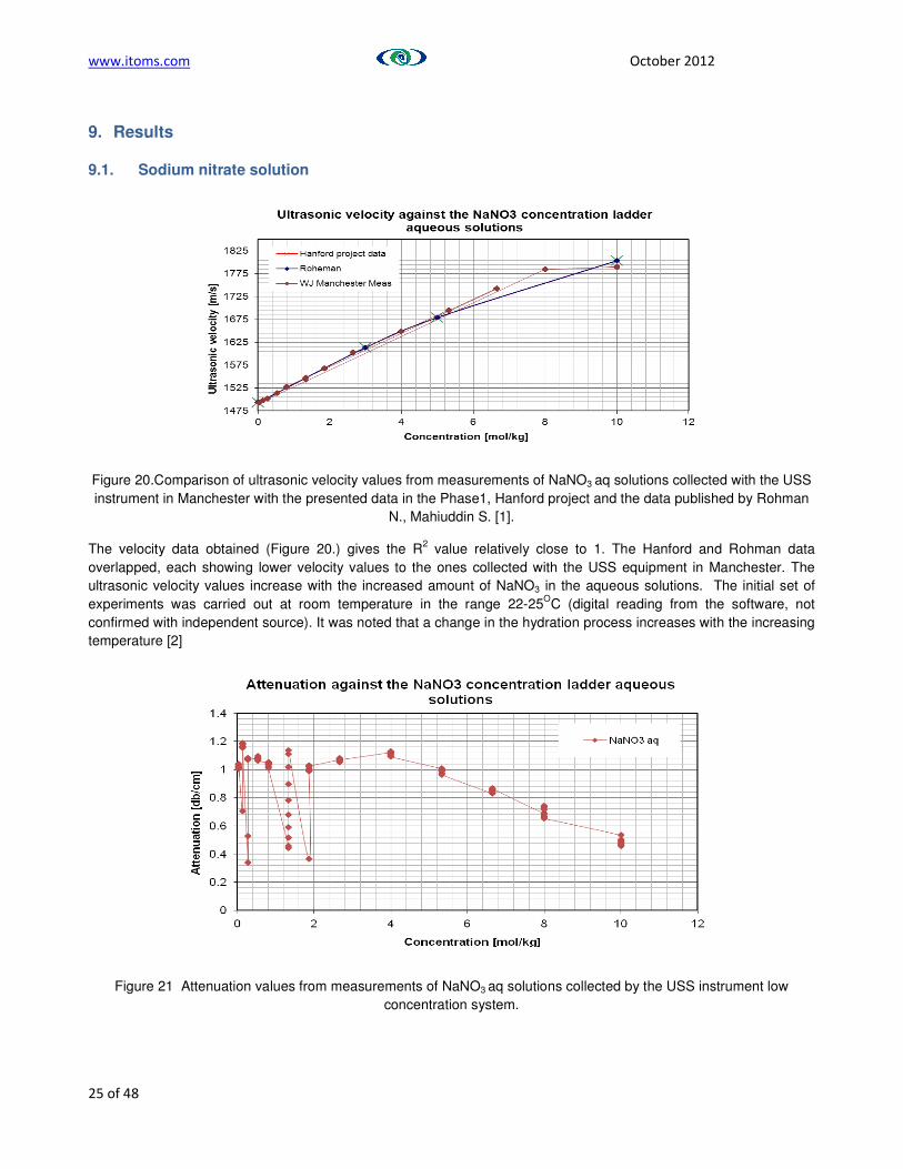
www.itoms.com October 2012
25 of 48
9. Results
9.1. Sodium nitrate solution
Figure 20.Comparison of ultrasonic velocity values from measurements of NaNO3 aq solutions collected with the USS
instrument in Manchester with the presented data in the Phase1, Hanford project and the data published by Rohman
N., Mahiuddin S. [1].
The velocity data obtained (Figure 20.) gives the R2 value relatively close to 1. The Hanford and Rohman data
overlapped, each showing lower velocity values to the ones collected with the USS equipment in Manchester. The
ultrasonic velocity values increase with the increased amount of NaNO3 in the aqueous solutions. The initial set of
experiments was carried out at room temperature in the range 22-25OC (digital reading from the software, not
confirmed with independent source). It was noted that a change in the hydration process increases with the increasing
temperature [2]
Figure 21 Attenuation values from measurements of NaNO3 aq solutions collected by the USS instrument low
concentration system.

www.itoms.com October 2012
26 of 48
The attenuation values of sodium nitrate are the attenuation values for a pure liquid and hence extremely low values.
They would appear to be lower than water and hence are extremely difficult to measure as pure liquids. Water in
particular is seen by many researchers to have too low a value to be measured accurately using through transmission
techniques.
9.2. Solid suspensions
The next step involved preparation of the suspensions in liquid phase (deionised water) and the appropriate powder
substance.
9.2.1. Suspension of aluminium hydroxide Al(OH)3 in water
Figure 22 Ultrasonic velocity values from measurements of Al(OH)3 aq suspensions collected by the USS instrument
low concentration system.
The analysis of the collected measurements (Figure 22) showed the multiple scattering occurring in the samples with
high concentration of aluminium hydroxide. The velocity values were increasing with the increase of the concentration
of the solid in a mixture.

www.itoms.com October 2012
27 of 48
Figure 23 Attenuation values from measurements of Al(OH)3 aq suspensions collected by the USS instrument low
concentration system.
The attenuation results for aluminium hydroxide (Figure 23) show a linear increase with attenuation suggesting that at the measurement frequencies there is no non-linear effects due to particle – particle interactions and that within the measurement time scale there was no sedimentation. During the measurement sedimentation did not occur in this sample.
9.2.2. Suspension of zirconium oxide ZrO2 in water
Zirconium dioxide samples were made up using the same concentration ladder as for aluminium hydroxide to compare the performance of the system with a high density material.
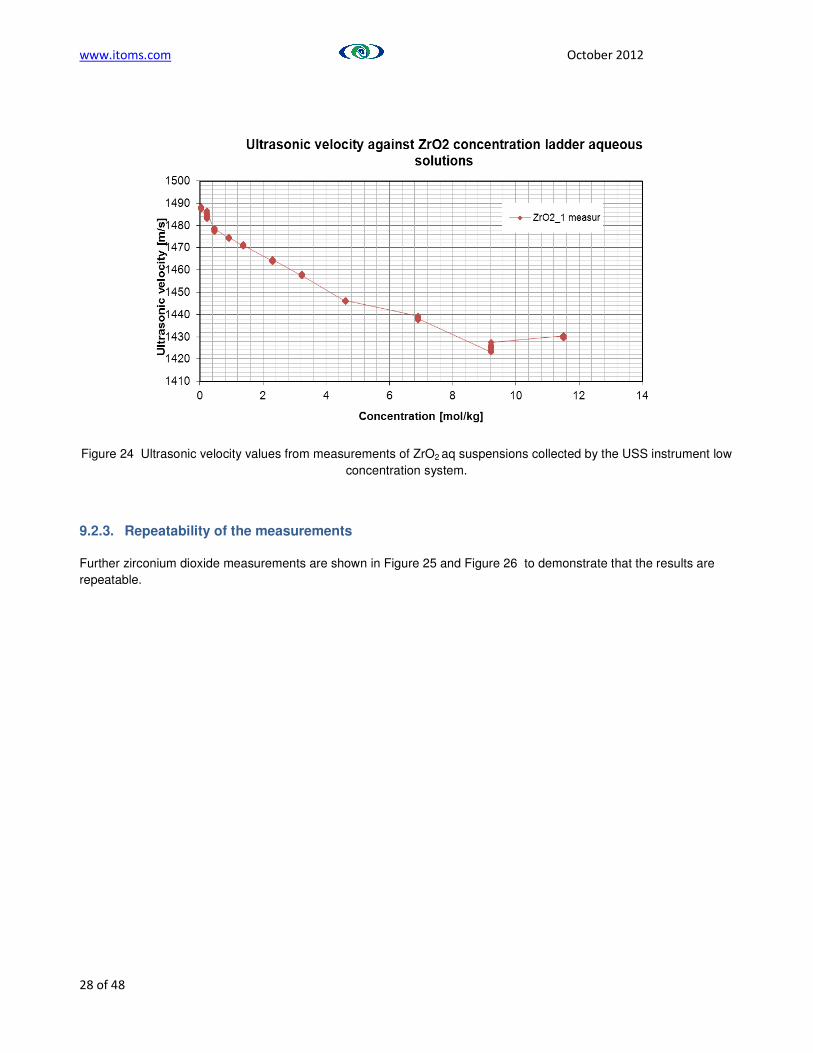
www.itoms.com October 2012
28 of 48
Figure 24 Ultrasonic velocity values from measurements of ZrO2 aq suspensions collected by the USS instrument low
concentration system.
9.2.3. Repeatability of the measurements
Further zirconium dioxide measurements are shown in Figure 25 and Figure 26 to demonstrate that the results are
repeatable.

www.itoms.com October 2012
29 of 48
Figure 25 Repeatability of the ultrasonic measurements of ZrO2 aq suspension collected by the USS instrument low
concentration system.
The measurements collected from the suspensions of zirconium oxide in water showed an inversely proportional
velocity to the concentration of the sample. The repeated experiment proved good reproducibility of the collected
results on the low concentration system. Multiple scattering in the high concentrated samples was also observed.
Figure 26 Attenuation measurements of ZrO2 aq suspension collected by the USS instrument low concentration
system.

www.itoms.com October 2012
30 of 48
Figure 27 Repeatability of attenuation measurements of ZrO2 aq suspension collected by the USS instrument low
concentration system.
9.2.4. Suspension of stainless steel (SS316) in water
Velocity results
Figure 28 Velocity measurements of stainless steel aq suspension collected by the USS instrument low
concentration system.

www.itoms.com October 2012
31 of 48
Attenuation results
Figure 29 Attenuation measurements of stainless steel aq suspension collected by the USS instrument low
concentration system.
9.2.5. Suspension of aluminum hydroxide in NaNO3aq solution
Figure 30 Ultrasonic velocity values from measurements of Al(OH)3 in NaNO3 aq suspensions collected by the
USS instrument low concentration system.

www.itoms.com October 2012
32 of 48
Figure 31 Attenuation values from measurements of Al(OH)3 in NaNO3 aq suspensions collected by the USS
instrument low concentration system

www.itoms.com October 2012
33 of 48
9.2.6. Complex powder mixtures in NaNO3 aqueous solution
The volume concentration of the Na(NO)3 was 13% and the bulk density was 1.17.
Solids Content required concentrations per mixture
Compound vol % Total solids
Gibbsite 52
Zirconium Oxide 37
Stainless Steel 11
Combine Stimulants 100
Table 3 The volume percentage for a solids used to prepare the complex mixtures. Attenuation values from
measurements of complex powders mixture in NaNO3 aq suspensions collected by the USS instrument Hi-C
concentration system.
Concentration of mixture [%] Total mass [g]
1 14.69
2 29.39
4 60.04
6 93.92
8 125.24
10 160.09
Table 4 Total amount of mixed powders used to prepare the complex samples

www.itoms.com October 2012
34 of 48
Figure 32 Ultrasonic velocity values from measurements of complex powders mixture in NaNO3 aq
suspensions collected by the USS instrument Hi-C concentration system
The bigger concentration of the sample the more tendency for particles to sediment, although the samples
were mixed with the visible vortex on top of the surface.
Figure 33 Attenuation values from measurements of complex powders mixture in NaNO3 aq suspensions
collected by the USS instrument Hi-C concentration system
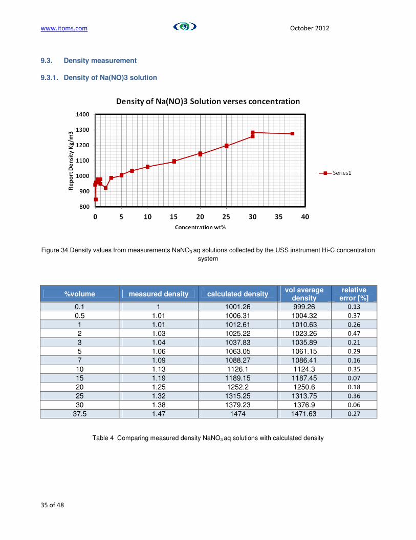
www.itoms.com October 2012
35 of 48
9.3. Density measurement
9.3.1. Density of Na(NO)3 solution
Figure 34 Density values from measurements NaNO3 aq solutions collected by the USS instrument Hi-C concentration
system
%volume measured density calculated density vol average
density relative
error [%]
0.1 1 1001.26 999.26 0.13
0.5 1.01 1006.31 1004.32 0.37
1 1.01 1012.61 1010.63 0.26
2 1.03 1025.22 1023.26 0.47
3 1.04 1037.83 1035.89 0.21
5 1.06 1063.05 1061.15 0.29
7 1.09 1088.27 1086.41 0.16
10 1.13 1126.1 1124.3 0.35
15 1.19 1189.15 1187.45 0.07
20 1.25 1252.2 1250.6 0.18
25 1.32 1315.25 1313.75 0.36
30 1.38 1379.23 1376.9 0.06
37.5 1.47 1474 1471.63 0.27
Table 4 Comparing measured density NaNO3 aq solutions with calculated density

www.itoms.com October 2012
36 of 48
Figure 35 Density values from measurements NaNO3 solution compared to the calculated value

www.itoms.com October 2012
37 of 48
9.3.2. Density of aluminium hydroxide suspension in Na(NO)3)
% volume measured density calculated density relative error
[%]
0.1 1.17 1.17166 0.14
0.5 1.18 1.17831 0.14
1 1.19 1.18661 0.29
2 1.2 1.20323 0.27
3 1.22 1.21984 0.01
5 1.25 1.25307 0.24
7 1.29 1.2863 0.29
10 1.34 1.33614 0.29
15 1.42 1.41921 0.06
20 1.5 1.50228 0.15
25 1.59 1.58535 0.29
Table 5 Comparing measured density of aluminium hydroxide in NaNO3 aq suspensions with calculated density
Figure 36 Density values for aluminium hydroxide in NaNO3 aq suspensions plotted against calculated values

www.itoms.com October 2012
38 of 48
9.3.3. Density of aluminium hydroxide suspension in water
% volume measured density calculated density relative error
[%]
0.1 1 1001.42 0.14
0.5 1.01 1007.1 0.29
1 1.01 1014.2 0.41
2 1.03 1028.4 0.16
3 1.04 1042.6 0.25
5 1.07 1071 0.09
7 1.1 1099.4 0.05
10 1.14 1142 0.18
15 1.21 1213 0.25
20 1.28 1284 0.31
25 1.36 1355 0.37
Table 6 Comparing measured density of aluminium hydroxide in water suspensions with calculated density.
Figure 37 Density values for aluminium hydroxide in water suspensions plotted against calculated values

www.itoms.com October 2012
39 of 48
9.3.4. Density of complex mixture in Na(NO)3
% volume measured density calculated density relative error
[%]
1 1.07 1200.398 10.86
2 1.024 1230.81 16.80
4 1.057 1294.207 18.33
6 1.047 1364.286 23.26
8 1.087 1429.074 23.94
10 1.101 1501.173 26.66
Table 7 Comparing measured density of complex mixture in Na(NO)3 solution with calculated density.
Figure 38 Density values for a complex mixture in Na(OH)3 solution plotted against calculated values
9.4. Review of original data
When reviewing the original data we found that the increasing solids loading and hence change in acoustic velocity
resulted in changes in the arrival time of the signal and a reduction in the magnitude of the pulse amplitude due to
attenuation.
As the pulse arrival time moved, the pulse echo signal moved in relation to the other echoes in the system. With a
sufficient shift in arrival time the pulse clashed with other echoes and was either lost or misdetected. This was

www.itoms.com October 2012
40 of 48
especially problematic as the amplitude of the pulse was reduced and the pulse became the same order of magnitude
as the noise. This caused the detector to falsely identify the wrong signal and hence the spectra become highly
variable.
10. Discussion
10.1. Ultrasonic velocity of constituent materials
McClements and Povey provide a useful application of the first principles scattering model to the phenomenological method, by splitting the scattering coefficients of the ECAH model between the effective compressibility and effective density of the Urick equations
[ ]10323Re
2
3AA
rkc
exc +−=φ
α
This allows the thermal and visco-inertial mechanisms to be related individually to the compressibility and density. Hence it is possible to show that the compressibility is linked to thermal effects
−⋅=
33
31
rk
Ai
c
o
eff
φκκ
And density is linked to visco-inertial effects
−⋅=
33
19
1rk
Ai
c
eff
φρρ
For less dense materials the thermal mechanism becomes important for both the attenuation and velocity components. This is demonstrated in the results where the aluminium hydroxide velocity has a negative velocity co-efficient with concentration, compared to the denser zirconium dioxide and stainless steel, which have positive co-efficients.
Hence, in the complex mixture, the effect of increasing stainless steel and zirconium dioxide concentration is offset by
the increase in aluminium hydroxide concentration - the result being that acoustic velocity is not a linear function of
overall solids loading.
10.2. The reflection coefficient
The reflection co-efficient method was proposed as a method of studying the density. However, experience showed
that the data was very variable and drifted over time.
effeffk ρκ
ω
.
1
*=

www.itoms.com October 2012
41 of 48
Plotting the value of the reflection coefficient against changes in density for a quartz delay line in a liquid (as shown
below), and comparing the change with the change in velocity for a similar density change, shows that the magnitude
of the relative change in reflection co-efficient is substantially smaller than the velocity.
Figure 39 The Effect of changing liquid density on the reflection coefficient and ultrasound velocity
This, coupled with the high sensitivity of the technique to disturbances on the face of the transducer, ie bubbles etc,
makes the method relatively noisy. It could be argued that using a fixed value of reflection co-efficient, and using the
measured forward velocity to produce a rough measure of density, would be as accurate. Since the ultrasound
velocity can be used to calculate solids loading directly through the equation this diminishes the usefulness of this
technique.
11. Conclusions
• Using ultrasound to detect the composition of complex mixtures is complicated by the presence of materials
in which the physical properties result in velocities which increase or decrease with concentration, hence
effectively cancelling out the impact of overall changes in solids loading on the ultrasound velocity
• The reflection co-efficient measurement is very ill posed with a high degree of sensitivity to noise and a
relative insensitivity to changes in density. The noise is due to the short range action of the wave in the liquid
and the relative small integration area of the transducer
• Using multiple reflective echoes from the back face of the transducer delay line would improve this but
requires more sophisticated measurement algorithms to identify the correct signals in the other echoes
• The diameter of the transducer has a large impact of the quality of the reflection measurement but the larger
transducer used was still not large enough to have sufficient integration
• Ultrasonic through transmission measurements will always be better than pulse echo in the same sensor
geometry

www.itoms.com October 2012
42 of 48
12. Recommendations for further work
• Further development of this method should concentrate on forward through transmission
measurements with separate transmit and receive transducer
• The larger the transducers the better for the measurements
• Using a high concentration measurement method such as the Hi-C version of the Ultrasound
Spectrometer would provide better data quality
• For reflectance measurements use a softer delay line material to reduce the impedance mismatch
between the delay line and the liquid and hence increase the reflection co-efficient sensitivity to
density changes.
Contact details
Dr. Richard Tweedie
Industrial Tomography Systems
Speakers House
39 Deansgate
Manchester
United Kingdom
M3 2BA
T: +44 (0) 161 832 9297
13. References
1. Roelant, D., 2001 FY2011 Project #1 Technical Report ask 15: Advanced HLW Instrumentation Ultrasonic
Spectroscopy Phase I Test Summary Report
2. Wang Y, Povey M., A simple and rapid method for the determination of particle size in emulsions from
ultrasound data Colloids and Surfaces B: Biointerfaces 12 (1999) 417–427
3. Rohman N., Mahiuddin S., Concentration and temperature dependence of ultrasonic velocity and isentropic
compressibility in aqueous sodium nitrate and sodium thiosulfate solutions, J.Chem.Soc.,Faraday
Trans.,1997,93(11), 2053-2056
4. V. Janėnas, V. Abaravičiūtė, V. Kasperiūnas, O. Majauskienė, R. Šaudienė, Investigation of water structure
changes in carbamide and nitrates [NaNO3, Ca(NO3)2, NH4NO3] solutions by ultra acoustic method, ISSN
1392-2114 ULTRAGARSAS, Nr.3(33). 1999
5. McClements D, Povey M 1889 Scattering of Ultrasound by Emulsions, J Phys D: Appl Phys 22 38-47

www.itoms.com October 2012
43 of 48
14. Appendix 1
Table 8 Composition of sodium nitrate solution
No of
sample
Conc
[v%]
Volume
[ml]
Density
[g/cm3]
NaNO3
[v]
NaNO3
[g]
NaNO3
[mol]
NaNO3
[mol/kg]
mass bulk
density
1 0.10 350.00 2.26 0.35 0.79 0.01 0.03 350.44 1.00
2 0.50 350.00 2.26 1.75 3.96 0.05 0.13 352.21 1.01
3 1.00 350.00 2.26 3.50 7.91 0.09 0.27 354.41 1.01
4 2.00 350.00 2.26 7.00 15.83 0.19 0.53 358.83 1.03
5 3.00 350.00 2.26 10.50 23.74 0.28 0.80 363.24 1.04
6 5.00 350.00 2.26 17.50 39.57 0.47 1.33 372.07 1.06
7 7.00 350.00 2.26 24.50 55.39 0.65 1.86 380.89 1.09
8 10.00 350.00 2.26 35.00 79.14 0.93 2.66 394.14 1.13
9 15.00 350.00 2.26 52.50 118.70 1.40 3.99 416.20 1.19
10 20.00 350.00 2.26 70.00 158.27 1.86 5.32 438.27 1.25
11 25.00 350.00 2.26 87.50 197.84 2.33 6.65 460.34 1.32
12 30.00 350.00 2.26 105.24 237.97 2.80 8.00 482.73 1.38
13 37.50 350.00 2.26 131.56 297.46 3.50 10.00 515.90 1.47

www.itoms.com October 2012
44 of 48
Table 9 Composition of aluminium hydroxide suspensions in water
Density of
Al(OH)3
[g/cm3]
Al(OH)3
[g]
Al(OH)3
[mol]
AL(OH)3
[mol/kg] bulk density2
2.42 0.85 0.01 0.03 1.00
2.42 4.24 0.05 0.16 1.01
2.42 8.47 0.11 0.31 1.01
2.42 16.94 0.22 0.62 1.03
2.42 25.41 0.33 0.93 1.04
2.42 42.35 0.54 1.55 1.07
2.42 59.29 0.76 2.17 1.10
2.42 84.70 1.09 3.10 1.14
2.42 127.05 1.63 4.65 1.21
2.42 169.40 2.17 6.21 1.28
2.42 211.75 2.71 7.76 1.36
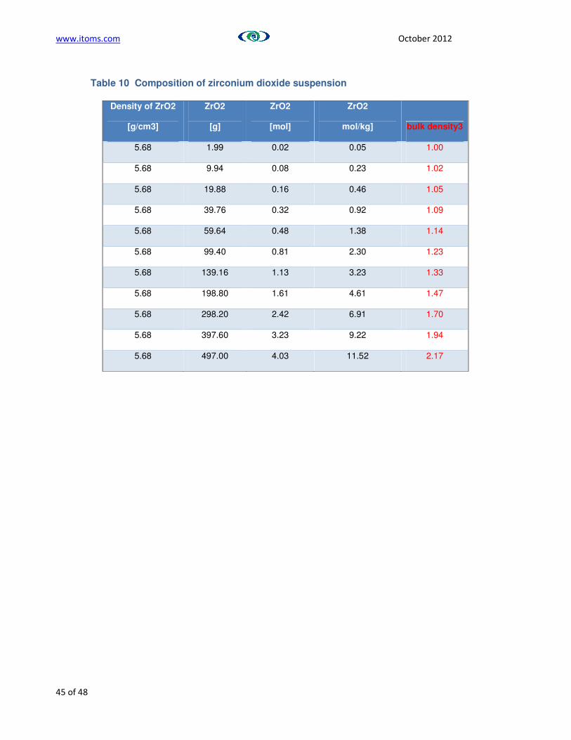
www.itoms.com October 2012
45 of 48
Table 10 Composition of zirconium dioxide suspension
Density of ZrO2
[g/cm3]
ZrO2
[g]
ZrO2
[mol]
ZrO2
mol/kg] bulk density3
5.68 1.99 0.02 0.05 1.00
5.68 9.94 0.08 0.23 1.02
5.68 19.88 0.16 0.46 1.05
5.68 39.76 0.32 0.92 1.09
5.68 59.64 0.48 1.38 1.14
5.68 99.40 0.81 2.30 1.23
5.68 139.16 1.13 3.23 1.33
5.68 198.80 1.61 4.61 1.47
5.68 298.20 2.42 6.91 1.70
5.68 397.60 3.23 9.22 1.94
5.68 497.00 4.03 11.52 2.17
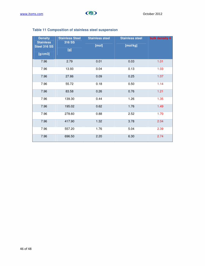
www.itoms.com October 2012
46 of 48
Table 11 Composition of stainless steel suspension
Density
Stainless
Steel 316 SS
[g/cm3]
Stainless Steel
316 SS
[g]
Stainless steel
[mol]
Stainless steel
[mol/kg]
bulk density 4
7.96 2.79 0.01 0.03 1.01
7.96 13.93 0.04 0.13 1.03
7.96 27.86 0.09 0.25 1.07
7.96 55.72 0.18 0.50 1.14
7.96 83.58 0.26 0.76 1.21
7.96 139.30 0.44 1.26 1.35
7.96 195.02 0.62 1.76 1.49
7.96 278.60 0.88 2.52 1.70
7.96 417.90 1.32 3.78 2.04
7.96 557.20 1.76 5.04 2.39
7.96 696.50 2.20 6.30 2.74
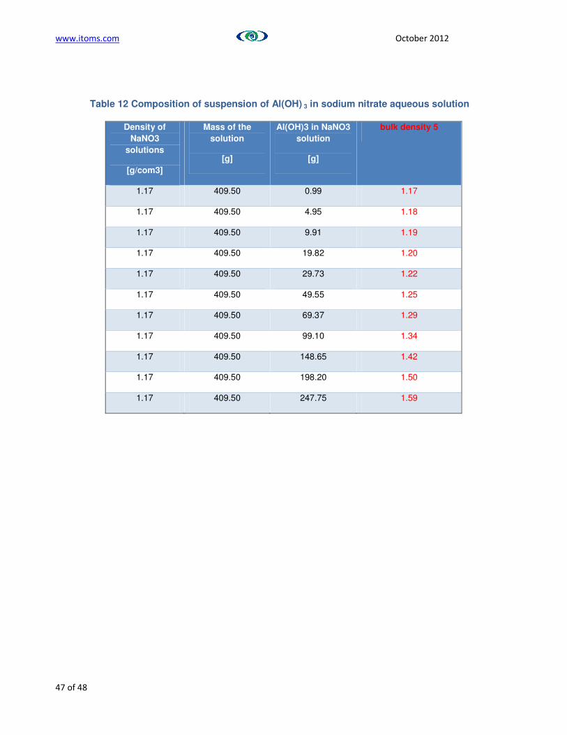
www.itoms.com October 2012
47 of 48
Table 12 Composition of suspension of Al(OH) 3 in sodium nitrate aqueous solution
Density of
NaNO3
solutions
[g/com3]
Mass of the
solution
[g]
Al(OH)3 in NaNO3
solution
[g]
bulk density 5
1.17 409.50 0.99 1.17
1.17 409.50 4.95 1.18
1.17 409.50 9.91 1.19
1.17 409.50 19.82 1.20
1.17 409.50 29.73 1.22
1.17 409.50 49.55 1.25
1.17 409.50 69.37 1.29
1.17 409.50 99.10 1.34
1.17 409.50 148.65 1.42
1.17 409.50 198.20 1.50
1.17 409.50 247.75 1.59
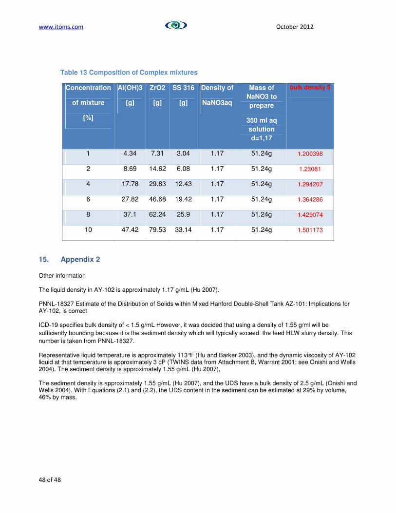
www.itoms.com October 2012
48 of 48
Table 13 Composition of Complex mixtures
Concentration
of mixture
[%]
Al(OH)3
[g]
ZrO2
[g]
SS 316
[g]
Density of
NaNO3aq
Mass of
NaNO3 to
prepare
350 ml aq
solution
d=1,17
bulk density 5
1 4.34 7.31 3.04 1.17 51.24g 1.200398
2 8.69 14.62 6.08 1.17 51.24g 1.23081
4 17.78 29.83 12.43 1.17 51.24g 1.294207
6 27.82 46.68 19.42 1.17 51.24g 1.364286
8 37.1 62.24 25.9 1.17 51.24g 1.429074
10 47.42 79.53 33.14 1.17 51.24g 1.501173
15. Appendix 2
Other information
The liquid density in AY-102 is approximately 1.17 g/mL (Hu 2007).
PNNL-18327 Estimate of the Distribution of Solids within Mixed Hanford Double-Shell Tank AZ-101: Implications for AY-102, is correct ICD-19 specifies bulk density of < 1.5 g/mL However, it was decided that using a density of 1.55 g/ml will be
sufficiently bounding because it is the sediment density which will typically exceed the feed HLW slurry density. This
number is taken from PNNL-18327.
Representative liquid temperature is approximately 113°F (Hu and Barker 2003), and the dynamic viscosity of AY-102 liquid at that temperature is approximately 3 cP (TWINS data from Attachment B, Warrant 2001; see Onishi and Wells 2004). The sediment density is approximately 1.55 g/mL (Hu 2007), The sediment density is approximately 1.55 g/mL (Hu 2007), and the UDS have a bulk density of 2.5 g/mL (Onishi and Wells 2004). With Equations (2.1) and (2.2), the UDS content in the sediment can be estimated at 29% by volume, 46% by mass.