child labor and schooling response to changes in coca ... · child labor and schooling response to...
TRANSCRIPT
1
Child Labor and Schooling Response to Changes in
Coca Production in Rural Peru
Ana C. Dammert*
McMaster University and IZA
Abstract
Coca eradication and interdiction are the most common policies aimed at reducing the production and distribution of cocaine in the Andes, but little is know about their impact on households. This paper uses the shift in the production of coca leaves from Peru to Colombia in 1995 to analyze the indirect effects of the anti-coca policy on children’s allocation of time. After different sensitivity checks, the results indicate that changes in coca production are associated with increases in work and hours children living in coca-growing states devote to work within and outside the household, with no effects on schooling outcomes. These findings suggest a previously undocumented indirect effect of drug policies on household behavior.
JEL Classification: J13, J22, O15, R23
Keywords: Child labor, Schooling, Coca Production, Peru
* Department of Economics, McMaster University, 1280 Main Street W, Hamilton, ON L8S 4M4, Canada. I would like to thank Dan Black, Jose Galdo, Jeff Kubik, Sonia Laszlo, and two anonymous referees for useful comments and suggestions. This paper also benefited from comments received at the NEUDC at Brown University, LACEA at the American University of Paris, and seminar participants at Queen’s and McMaster University. Any errors and omissions are my own.
2
I. INTRODUCTION
During the 1980s and mid-1990s, Peru was the leading producer of coca leaves,
providing 60 to 70 percent of international coca trafficking requirements, while Colombia was
the main producer of refined cocaine (UNDCP 2002). As a result, coca eradication and
interdiction are the most common policies aimed at reducing the production and distribution of
cocaine. Peru implemented the so-called “air-bridge” denial between Peru and Colombia in 1995
where local militaries took control of airports and ports in coca regions. This policy was also
accompanied by the dismantling of the powerful Cali cartel in Colombia. Prices declined below
production costs and farmers started abandoning their coca fields in Peru while in Colombia drug
traffickers demanded large-scale homegrown crops. Estimates suggest that coca leaf production
declined by 66 percent in Peru and shifted towards Colombia. Very little is known about the
effect of the negative change in coca production on children’s time allocation in rural areas,
where most of children work. The only evidence shows that the positive demand shock increased
self-employment earnings and labor supply of teenage boys in rural Colombia (Angrist and
Kugler 2005). The main purpose of this paper is to use this shift to examine whether the coca
economy has an effect on child labor and schooling in Peru.
Understanding how exogenous shocks affect education and child labor (defined as
children engaged in market work) is important for several reasons. One of the main features of
child labor in developing countries is that a large share of children in rural areas works in
agriculture (Edmonds and Pavnick 2005a). In Peru, 93 percent of economically active children
were engaged in agriculture in 1994. Additionally, coca was a relevant source of agricultural
employment and income in the 1990s. In 1995, about 200,000 households had an economy based
on coca production or activities related to it (INEI 2000). Even though the price of raw coca leaf

3
makes up a small fraction of the price of cocaine, it is higher than for legal crops and most
estimates suggest that coca cultivation played an important role in the economy (Steiner, 1998). 1
Critics of drug interdiction and eradication argue that these policies have substantial
economic costs for rural producers (Thoumi 2002, Cotler 1999). Theoretical and empirical
evidence have shown that when family income decreases there will be less child leisure, less
school, and more child work. For example, the Basu and Van (1998) seminal model show that
the household will send children to work if adult income or family income from non-child labor
sources becomes very low. A poor household cannot afford to consume the good of child leisure
but it will as soon as adult income rises sufficiently.
Other factors might play a role as well. For example, wages and child labor might decrease
in states that are more exposed to coca production and experience larger declines in demand.
Another scenario, however, could be that farmers to shift toward less skill-intensive crops where
the demand for child labor increases.2 Likewise, changes in the return of education as a
consequence of the anti-coca policies affect child labor and schooling but it could go either way.
If households switch to other crops where higher education is needed, the expected returns to
schooling increase and there will be more schooling and less work. The loss of revenues and
rents from coca production might affect local public finance altering the quality of education and
worsening returns to education.
Ultimately, the net effect of changes in coca production on child labor and schooling
depends on the relative strength of these channels. The existing empirical literature suggests a 1 Estimates regarding how much revenue Peru received annually from the drug trade during this period range from US$800 to US$550 million (Steiner, 1998). 2 One of the main problems is that for most children working in rural farms or family enterprises, wages are not observable. Different alternatives have been used such as estimating a family farm production function where the marginal productivities of labor are a measure of shadow wages (Jacoby and Skoufias 1997). Another empirical strategy is to exploit variation in economic conditions, as these will alter the wage or value of children’s time. For example, empirical evidence has shown that financial crisis leads to higher child labor especially among the poor and younger children (Funkhouser 1999, Skoufias and Parker 2006, Rucci 2003).

4
negative association between increases in rice prices caused by trade liberalization and child
labor in Vietnam, this effect varies across children that differ in their households’ exposure to
rice prices as consumers and producers with income playing an important role (Edmonds and
Pavnick 2005b). But also there is evidence that higher coffee prices caused by market
liberalization in Nicaragua increases child labor, so that the dominant effect of rising coffee
prices is through labor demand (Kruger 2004).
Using data from the Peruvian Living Measurement Survey (PLSMS), I compare the
response of child labor and schooling before and after the anti-coca policy for a group of children
living in states able to cultivate coca leaves (treatment group) to a group living in states that were
not able to produce coca leaves due to climate, soil conditions, infrastructure, and other
environmental conditions, and thus not affected by the change in policy (comparison group).
After several sensitivity checks, the estimates suggest that changes in coca production are
associated with large increases in child labor. In particular, child labor increased in coca-growing
states by 18 and 40 percent in 1997 and 2000 respectively, with no effect on schooling outcomes.
While labor force participation increased more in 2000 than in 1997, the effect on the intensity of
work both inside and outside the household was higher in 1997. Likewise, there are increases in
wage work for male adults with more than primary school with small effect on participation for
men with less than primary school. The data also shows that the increase in market work for
children is not caused by increased in wage work, but it is operating through increases in
agricultural work where 96 percent of children are non-remunerated workers in the family farm.
Results suggest that children are not working in the formal market as substitutes for unskilled
labor; rather the increase in market and domestic work appears as children filling in for working
parents. In addition, schooling cost appears to play a role in households where children can not

5
work in the family enterprise or farm to buffer the negative shock in adult labor demand. These
findings suggest a previously undocumented indirect effect of drug policies on household
behavior.
The remainder of the paper proceeds as follows: the next section presents the institutional
background information; Section III outlines the econometric methodology and describes the
data used in the empirical section; Section IV presents the regression results; Section V discusses
several factors that may influence the interpretation of the results in this study; and finally,
Section VI offers concluding comments.
II. INSTITUTIONAL BACKGROUND
Changes in coca production have important attributes.3 First, coca cultivation is based on
climate, soil, infrastructure, and other environmental conditions. The coca bush is a crop that
prospers especially between 600 and 2,000 meters above sea level and in the lower tropical
rainforest regions of the Andes.4 Second, households with children are no more likely to cultivate
coca than households without children are. Neither the activities of children nor their presence
influence coca cultivation. It is part of a tradition among Andean peasants. Before the 1970s, the
production was exclusively for chewing, alternative medicine, and ritual ceremonies, all
classified as “traditional legal use” by the United Nations in 1988. With the increasing demand
for drugs, however, coca leaves acquired an important value as the principal input in the
production of cocaine.
3 Throughout this paper coca production refers to production of raw materials (coca leaves) and not the production of cocaine. 4 It belongs to the Erythoxylon genotype that includes around 250 species but only two contain cocaine, which are mainly cultivated in Peru and Colombia (UNDCP 2003).
6
Third, coca farming is the most labor-intensive stage of cocaine production. In addition to
clearing and preparing the fields for planting the coca seedlings, coca farming may require
weeding, pruning, and manual hoeing before plants reach maturity. The first collection of leaves
takes place six months after planting, and large amounts of labor are required for picking the
leaves, drying, and transporting them to local markets (Riley 1996, Morales 1989).5 In 1995,
about 200,000 households had an economy based on coca production or activities related to
(INEI 2000). Even after the introduction of counter-narcotics policies in 1995, coca farming still
represents a large fraction of income for peasants. For example, it represents 48 percent of total
net family income in the basin of the Apurimac River where most coca is harvested in 2000
(Bedoya, 2003).
Finally, until 1995 Peru was the leading producer of coca leaves. In 1989, Peru produced
about 186,300 hectares, followed by Bolivia with 78,300 hectares and Colombia with 33,072 for
a total of 297,672 hectares (UNODC 1999).6 Moreover, 60 to 70 percent of international coca
trafficking requirements were supplied by Peru (UNDCP 2002). While Peru and Bolivia were the
main producers of coca leaves in the 1980s and 1990s, Colombia was the principal exporter and
producer of coca paste and cocaine with a share of nearly 40 percent of the world supply of
cocaine (UNODC 1999).
5 Peasants sell dried coca leaves for the production of coca paste, which uses a simple process that takes four to five days. This second stage involves maceration to separate the alkaloid cocaine from the leaves using kerosene and other organic solvents. On average, about 341 kilos of coca leaves mixed with different chemicals and water make 3 kilos of coca paste (Morales, 1989). Most of this coca paste is shipped to Colombia or local urban areas to illegal laboratories to produce coca base, obtained by removing impurities and concentrating alkaloid content (Riley 1996). The final stage consists of the refinement of coca base to produce cocaine hydrochloride: on average 3.8 kilos of coca paste yield 1 kilo of cocaine (Morales, 1989). 6 Due to illegality of coca production, available data on this crop is scarce or underestimated. International organizations started collecting this data in the mid-1980s. Data before 2001 is from the United Nations Office for Drug Control and Crime Prevention (UNDCP). Estimates of the cultivation of coca bush and production of coca leaf are drawn from various sources including Governments, UNDCP field offices, and the United States Department of State’s Bureau for International Narcotics and Law Enforcement Affairs. From 2001, the UNDCP has collected data through aerial photographs.

7
In 1993, US policy shifted interdiction away from Caribbean transit zones toward
stopping cocaine production in the Andes. As a result, in 1995, the Peruvian Government, with
financial aid from the US Government, launched the National Plan for the Prevention and
Control of Drugs, which among other things instituted the “Denial Bridge” or interdiction of
illegal airplanes and boats between Peru and Colombia.7 At the same time, in 1995 the
Colombian Cali cartel collapsed, which was one of Peru’s largest customers. Consequently, the
production of the coca leaf declined with the abandonment of about 60 percent of the total
cultivated area of coca (UNDCP 2002). Between 1995 and 1998, the area cultivated of coca leaf
recorded a rapid growth in Colombia, displacing the Peruvian supply to second place (Figure 1).
As opposed to Plan Colombia, Peru does not allow the use of chemical spray to fumigate
coca crops with herbicides. Instead, it has mixed manual eradication with schemes to encourage
peasants to pull the crop up and plant legal alternatives. However, producing alternative products
is not profitable. For example, in 2004 prices, a hectare of coca yields an annual income of up to
$7,500, compared with $600 from coffee or $1,000 from cocoa.8 It is important to note that in
Peru it is legal to cultivate coca if peasants sell coca leaves exclusively to the National Enterprise
of Coca (Empresa Nacional de la Coca -ENACO).9 In 1998, ENACO registered only 2,341
metric tones of coca or 2.5 percent of the 95,000 metric tones produced. That means that 97.5
percent of the total production was illegal. It is not profitable to sell coca leaves to ENACO,
7 The National Plan for the Prevention and Control of Drugs Plan 1994-2000 (Decree Number 824) defined the roles of the Peruvian military and police in counter-narcotics efforts, among others it establishes the “Bridge Denial” where Peruvian National Police assumes total control of airports and ports in coca areas, it allows the destruction of illegal airports and created the Peruvian Air Force (FAP) Aerial Intercept Program that denies traffickers the ability to transport cocaine base by air and the Peruvian Navy Intercept that halts traffickers on rivers. It also established the promotion of coca crop substitution. 8 See www.devida.gob.pe 9 The line between "legal" and "illegal" coca is not clear since it is not well defined which crops are permitted and which are not. Moreover, traditional coca growing areas are not specifically mapped out with the exception of the Convencion-River Valley where ENACO is headquartered.
8
which offers a lower price. For instance, in the Apurimac-Ene basin ENACO bought coca leaves
at US$1.12 per kilo, while the black market offered US$1.40 per kilo in 1999.
The identification strategy relies on an exogenous shift in coca production caused by
counter-narcotics policies. Angrist and Kugler (2005) use this variation to explain changes in
adult and teenage labor in Colombia, and they find small effects. As they acknowledge, however,
one of the main problems with their study is that they cannot disentangle the effect of increased
coca production from a secular increase in rural insurgent activity. The analysis for Peru,
however, does not suffer from this problem since the insurgent activity from Sendero Luminoso
(Shining Path) has declined drastically since 1993.
III. DATA AND EMPIRICAL METHODOLOGY
Data
This study compares the child labor and schooling status of children who reside in coca-
growing states to children living in non-growing states. The data used come from the Peruvian
Living Standard Measurement Survey (PLSMS). The PLSMS was conducted by the Peruvian
non-profit organization Instituto Cuanto S.A. with assistance from the World Bank. The survey
is nationally representative and the sample is stratified into geographic regions. It collects
information about household characteristics and individual information for all family members
aged 6 years and above.10 Therefore, it allows the estimation of the labor supply of children aged
6 to 14 years without including older children with different skills and labor attachments and,
under most definitions, not viewed as child labor.
10 For a sub-sample of the data, the PLSMS consists of rotating panels. I did not exploit the panel here, since there are concerns about nonrandom attrition and small sample size.

9
Children’s activities are grouped into domestic and market work. Domestic work includes
housekeeping and caretaking activities within the child’s own household such as cleaning,
cooking, taking care of siblings, among others. Market work includes wage employment, self-
employment, agriculture, unpaid work in a family business, helping in the family farm, among
others.11 Child labor refers to children engaged in market work.
The PLSMS spans the period of decline in coca leaf production and the implementation
of counter-narcotics policies. The first survey was conducted between May and August 1994, the
second survey between July and September 1997, and the third survey between May and June
2000. Thus, I use 1994 as the year before the implementation of the policies, whereas 1997 and
2000 correspond to years after the policies.
Table 1 presents summary statistics for the outcome measures and main individual
characteristics for the 1994, 1997, and 2000 cross-sectional surveys. The focus of this study is on
rural children, because they are the group more likely be affected by changes in policies related
to coca farming. The first column in table 1 presents summary statistics for the pooled sample.
Of the 5,450 rural children aged 6 to 14, half are male, 94 percent are enrolled in school, and 43
percent are employed in market work.12 On average, children have 3.2 years of completed
schooling and spend 6.4 hours a week in market work and 7.2 hours a week in domestic work.
Most children who work combine it with school, using Peruvian data for 1991, Patrinos and
Psacharopoulos (1997) find that child labor affects age-grade distortion for indigenous children
11 The questions asked are: “Did you work last week as a dependent for an enterprise, government, or self-employment? Did you work last week as self-employed, non-paid apprentice, or helping in a family farm?” These questions did not change across years. 12 The International Labor Organization distinguishes between child in economic activity and child labor. The former is a broad concept that encompasses most productive activities by children, including unpaid and illegal work as well as work in the informal sector. The latter is a narrower concept excluding all those children 12 years and older who are working only a few hours a week in permitted light work and those 15 years and above whose work is not classified as “hazardous” (ILO 2002). Using household surveys it is not possible to distinguish between hazardous and non-hazardous work.
10
but not for the whole sample. The authors hypothesize that Peruvian children can combine
school and work without negative effects because this extra income makes it possible to attend
school.
Empirical Methodology
The parameter of interest in assessing the impact of a policy is the effect of treatment on
the treated, which compares the outcome of interest in the treated state ( 1Y ) with the outcome in
the untreated state ( 0Y ) conditional on receiving treatment. If we could observe ( 0Y , 1Y ) for
everyone, the gain of being in the program is 1 0Y Y∆ = − . The evaluation problem is that these
outcomes cannot be observed for any single individual in both states, the treatment indicator can
take either the value 0 or 1 but not both. Assessing the impact of any policy requires making an
inference about the outcomes that would have been observed for people affected the policy had it
not been implemented. In absence of a controlled, randomized assignment, no direct estimate of
the counterfactual outcome is available. Instead, the outcome of people not affected by the
policy, or comparison group, proxy for the missing counterfactual. One commonly used non-
experimental estimator is the difference-in-difference estimator, which compares the change in
outcomes in the treatment group before and after the policy to the change in outcomes in the
comparison group.
The objective of this paper is the identification of the average effect of anti-coca policies
on child labor and schooling in states in which coca is harvested. In particular, compare child
labor and schooling outcomes in states that are affected by the anti-coca policy to the
counterfactual, which is child labor and schooling in coca-growing states had the policy not been
implemented. At a given point in time, however, a child is observed to be in either a coca-
growing state or a non-growing state. This paper uses an exogenous counter-narcotics policy that
11
leads to a shift in coca production from Peru to Colombia, where most coca is now harvested, to
identify the missing counterfactual. The identification strategy exploits the fact that counter-
narcotics policies affect people in rural areas living in states that based on climate, soil,
infrastructure, and other environmental conditions who are able to cultivate coca leaves
(treatment group), and compare them to children living in states who were not able to do so
(comparison group).
Formally, the difference-in-difference model estimates the average treatment effect on
the treated as a linear regression model:
' 97 2000 97 20001 2 3 1 2 1 2 ijt ijt j jt jt ijtY X C T T C T C Tγ γ γ ϕ ϕ θ θ ε= + + + + ++ + (1)
where i is an index for an individual ith living in state j in year t.13 The dependent variable Yijt
reflects the outcome of interest such as whether the child is employed or not, hours worked,
domestic work, school attendance, among others. Xijt is a vector of demographic variables. Cj is a
dummy variable, which equals 1 if state j is coca leaf producer and 0 otherwise, 97T and
2000T represent year dummies for the after period.
An 8-state growing region, as identified by the Peruvian National Plan for the Prevention
and Control of Drugs Plan of 1994, defines the distinction between coca-growing and non-
growing states. The idea is to remove the bias in the simple difference before and after for the
treatment group by subtracting the difference for the control group. The estimation of 1θ and 2θ ,
which are associated with the interaction of the treatment dummy and a dummy indicating the
after year, give us the net effect of changes in coca production for 1997 and 2000. The
difference-in-difference estimator controls for systematic differences across both states and time.
13 Alternatively, I could use a probit model to estimate employment probabilities. The results are not sensitive to the choice of assumption about the regression error distribution.

12
In other words, the estimator compares child labor and schooling within states for children
before and after the policy and differences in time-invariant community characteristics, while
comparing coca-growing states with non-growing states differences in changes that are not due
to coca farming. This estimation, however, may yield biased estimates if there are omitted or
unobserved state characteristics correlated with the error term. For instance, coca-growing states
may have lower economic growth and fewer employment opportunities for reasons not linked
with the reduction in coca production. For that reason, I include state fixed effects in equation
(1). To take into account the level of aggregation of the analysis, all standard errors are clustered
at the state-survey round to correct for potential correlated error terms.14
The key identifying assumption is that the change in the outcome of interest in
comparison areas is an unbiased estimate of the counterfactual. While I cannot directly test this
assumption, I can test whether the treatment and comparison groups are comparable in
observable characteristics. If they have different characteristics before the policy, the differences
between outcomes can be attributed to two factors: pre-existing differences (selection bias) and
the impact of the policy. Since treatment and comparison groups are not selected randomly, we
need a comparison group with similar characteristic to the treatment group, where child labor
would not have had differential trends in coca-growing states had the policy not taken place. To
formally test that the pre-policy time trends for the comparison and treatment group are not
different, I estimate equation (1) only for observations in the pre-policy period. Table 1 presents
summary statistics and difference in outcomes for children before the implementation of the
14 The identification strategy can be illustrated using a simple two-by-two differences table. Unreported estimates indicate that in the year prior to the policy there were small differences in child labor in coca-growing and non-growing states. In both types of regions, average employment rates increased in 1997 but employment increased more for children living in coca-growing states than for children living in non-growing states. In 2000, average employment rates increased for children living in coca-growing states but decreased for children living in non-growing states relative to 1994 (albeit not significant).
13
policy using the PLSMS survey for 1994. Children in both control and comparison groups are on
average 10 years old, with 3 years of completed schooling, and 48 percent are male. Estimates
show that we cannot statistically reject the hypothesis that the characteristics are the same for
both the control and comparison group at conventional levels of statistical significance, with the
exception that children in the treatment group work more in market activities (0.41 vs. 0.35) and
live with younger heads of household (42 vs. 44 years old).15
IV. COCA PRODUCTION, CHILD LABOR, AND SCHOOLING
Table 2 (column 1) presents estimates of equation (1) including state fixed effects.16 The
estimates suggest that children living in coca-growing states had a higher probability of engaging
in market work compared with children living in non-growing states. For instance, the
probability of working increased by 7 and 15 percentage points in 1997 and 2000, from an
overall participation of 38 percent in 1994. Thus, changes in coca production account for an
increase of approximately 18 percent (0.07/0.38) and 40 percent (0.15/0.38) in the probability of
working in 1997 and 2000 respectively.
One potential concern is whether differences in child labor are driven by factors that are
independent of changes in coca production. The identification assumption implies that the
inclusion of covariates, controlling for demographic and household characteristics, should not
alter estimates substantially. To address this, Columns 2 through 4 control for other covariates
15 Unreported summary statistics using data from the 1993 Population Census and the 1998 School Census show that coca-growing states are more rural than the rest of Peru. The coca-growing population is 47 percent rural, in comparison to 35 percent rural in the rest of the country. Non-growing states have similar primary and secondary school enrollment. In 1993, rural areas comprise 58 percent of total schools in Peru where the majority of schools are financed by the central government with a higher share in primary school (98 percent are public schools). Using School Census data for 1998 the results show that rural public schools have similar water and electricity infrastructure. Schools in non-growing states, however, are slightly better off. Results are available upon request. 16 I also estimate equation (1) for a sample excluding rural Lima (capital) and results are very similar to the reported with the entire sample.

14
that could explain the variation in child labor. Column 2 includes child characteristics to control
for age-gender differences. It also includes harvesting time with an indicator that is one if the
interview took place during the harvest. Coca crops can be harvested 3 to 5 times a year, which
are closely related to climatic conditions. The first harvest is carried out between February and
March (the period of highest rainfall), the second between May and June, and the third between
August and September. In November and December, the harvest is less productive since it
coincides with the dry season (UNODC 2002). Including these covariates, the estimates are
within a 95 percent confident interval of the estimates in Column 1 and the significance level
does not change.
I also take into account differences across regions, for instance, rural regions located on
the coast may produce export goods such as cotton and sugar, while rural areas in the highlands
produce food goods oriented to self-consumption that are less profitable. Moreover, changes in
the returns to schooling may vary across regions. These unobserved, region-specific
characteristics might bias the effects on child labor. For that reason, Column 3 includes dummy
variables indicating region (coast, highlands, and jungle) interacted with time to allow for
differential effects across years. The estimates show an insignificant change for 1997 and no
change for the interaction of coca-growing state and year 2000.
Column 4 controls for head of household characteristics and land ownership. Parental
education is a well-known determinant of child labor: parents that are more educated value
education more highly than parents with no schooling do, so children in educated households
will not work or work for fewer hours. Likewise, older parents will value more child labor than
younger parents who can work more hours or in multiple jobs. In addition, a family with land
holdings has incentives to use children’s work in the family farm or enterprise. They are also
15
more likely to be affected if farming is the main income source for the household (Bhalotra
2000). Including these covariates, the estimates show no significant changes in the interaction
coefficient of coca-growing state and year.
Previous work on Peru has showed that teenage girls spend significant time taking care of
younger siblings in the household and less time in school (Levison and Moe 1998). If the child
starts extensive household responsibilities, she would appear as not working and could distort the
results (Edmonds and Pavnick 2005a). The survey allows us to broaden the definition of work to
include domestic work. Domestic work is an indicator that takes the value of 1 if the child is
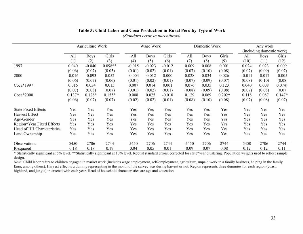
engaged in more than 7 hours of domestic work a week. Table 3 shows that the probability of
domestic work increased by 8 and 13 percentage points in 1997 and 2000, which represents and
increase of 13 percent (0.08/0.63) and 21 percent (0.13/0.63), respectively. In 2000, the policies
account for 28 percent (0.20/0.71) of the increase for girls and 13 percent (0.07/0.55) for boys. In
addition, Table 3 shows that the coefficient on the interaction term is positive in the case of
agriculture work and positive (albeit insignificant) for wage work. That is, all else being equal,
changes in coca production are associated with higher probability of working in agricultural
occupations and engaging in domestic work. In addition, I include domestic work in the
definition of child labor (column 10 -12), as before the coefficient on the interaction between
coca-growing state and time is positive and statistically significant for 2000. The patterns in the
data are consistent with gender differences in the allocation of time found in previous studies of
Peru (Ersado 2005, Ilahi 2001, Levison and Moe 1998, Ray 2000). Boys generally are more
active in market work while girls are more active in domestic work.
16
Hours Worked
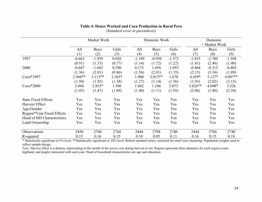
Table 4 shows the estimates using total weekly hours worked in market work and
domestic work as dependent variables to analyze the effects of anti-coca policies on the intensive
margin of child labor. Each column header indicates the dependent variable. The estimates
suggest that even though more children are engaged in market work in 2000, the change in hours
in market work is slightly higher in 1997 than 2000. On average, weekly hours worked in market
work of children in coca-growing states increased by 2.6 and 2.0 hours in 1997 and 2000,
respectively. In terms of domestic work, for boys the effect on hours worked is higher in 1997
than 2000, while for girls it is the opposite (albeit insignificant).
Including both domestic and market work, the estimates suggest girls in coca-growing
states spent 4.0 and 3.3 more hours a week engaged in wage and domestic work in 1997 and
2000. Hours worked increased for boys as well by 5.1 and 4.1 hours a week in 1997 and 2000.
Since most children are enrolled in school, an increase in hours worked corresponds to a
decrease in time spent studying, playing, or sleeping, which might undermine the effectiveness
of child attendance for children that work and attend school.
Schooling Outcomes
Most studies of the link between child labor and schooling find a negative correlation
between the two, but they point out that some types of work are compatible with schooling.17
Therefore, the observation that a decline in coca production is associated with higher child labor
does not necessarily imply a decrease in attendance rates. Schooling results are in Table 5. In
column (1) through column (3), the dependent variable is an indicator for whether a child is
17 See Edmonds (2007); Basu and Tzannatos (2003); Brown, Deardoff and Stern (2001); Bhalotra and Tzannatos (2003) for an extensive review.

17
currently attending school. Attendance decreased by 3 percentage points in 1997 in coca-
growing states, with higher effects for boys than for girls. As pointed out before, Peru has high
school enrollment rates; for that reason, it is not surprising that attendance rates did not change
much in coca-growing states after the introduction of anti-coca policies.
It is well documented, however, that even though school enrollment rates are high in
Peru, rural children have higher repetition rates and lower retention and student achievement
than urban children do, but there is not much variation within rural areas (World Bank, 2001).
Attendance rates, however, does not capture time spent in school or time spent learning. For that
reason, Table 5 includes other variables to analyze possible effects on school attainment. In
column (4) through column (6), the dependent variable is the highest level attained by the child.
The result shows a positive effect in 1997 and negative for 2000, albeit in both cases it is not
statistically significant. Other variable used in the literature to capture late entry and high failure
rates is an aggregate index of age-grade distortion or over-age indicator.18 This indicator
measures if the child under consideration had a normal progress (in terms of schooling years)
relative to his current age (Patrinos and Psacharopoulos 1997). Column (7) through column (9)
shows no statistical effect on over-age for children in coca-growing states. Unfortunately, in this
paper it is not possible to identify additional school outcomes since information about repetition
is only available in the 1994 PLSMS and there is no additional information about school
performance. The Peruvian Ministry of Education has test scores only for a selected sample in
urban schools for 1996 and 1998. In 2001, the sample of schools increased to incorporate rural
areas.
18 The index of age-grade distortion is defined as SAGE= [years of education/(age-6)]*100 and equal 100 for children aged 6 and currently attending school. Over-age indicator equals one if SAGE<100 and 0 otherwise.
18
V. ROBUSTNESS ANALYSIS
Panel A of Table 6 divides children in coca-growing states by whether they are living in
urban or rural areas. The definition of employment is the same as before (market work), but it
does not consider children working in agricultural occupations in urban areas. The idea here is to
check whether the interaction of the growing states*post-year is larger in rural than urban areas
of coca- growing states, since it is expected that shocks generated by the coca policy are larger in
the rural area. For that reason, I pooled the urban and rural sample and estimate equation (1)
allowing for main effects and interactions with both coca-growing state and year dummies. The
regression includes state fixed effects and controls for age, gender, harvest time, region*year of
the survey, and characteristics of the household head (age and education). The coefficient of
interest, the interaction of the coca-growing state*year, is allowed to differ by urban-rural status.
The estimates show that the interactions coca-growing state*year*rural are similar to
those generated using only rural data: the probability of enter into market employment is higher
in 2000 but the intensity of work, both in market and domestic work, is higher in 1997. For urban
areas, the estimated effect for labor outcomes is small suggesting that the policy had little impact
on urban children working in non-agricultural occupations in coca-growing states.
Panel B of Table 6 divides rural children in the coca-growing states by whether they
reside in agricultural households.19 All children in non-growing states are again the comparison
group. The idea here is to check whether the interaction of the growing states*post-year is larger
for children living in agricultural households than non-agricultural households of coca-growing
states. Since the policy affects directly households that grow coca leaves, it is expected that
shocks generated by the coca policy are larger for them. It is important to consider, however, that
19 Agricultural household is defined as one where the head of household works primarily in an agricultural occupation.
19
other households involved in the coca economy also are affected, for example producers of coca
paste and suppliers of intermediate inputs. Estimates show that the anti-coca policy affected
similarly labor outcomes of children living in agricultural households and non-agricultural
households in 1997. On the contrary, the change in the probability of entering into market work
is higher for children living in agricultural households, together with higher work hours in
market and domestic work in 2000. The effect on schooling is negative for all and statistically
significant for children living in non-agricultural households.
Panel C of Table 6 divides rural children in the coca-growing states using categories of
parental education as an indicator of permanent income to test whether poor households are more
affected by anti-coca policies.20 All children in non-growing states are again the comparison
group. Low education refers to households where the highest level of education obtained by the
head of household is primary (6 years of schooling) or less. Middle refers to households where
the head of household obtained more than primary but less than a secondary degree (between 7
and 10 years of schooling), and High refers to households where the head of household obtained
at least a secondary degree (11 years of more of schooling).
Evidence shows that poor and middle-income children are more likely to enter into
market employment while those from higher-income families are not negatively affected.
Changes in coca production causes a 40 percent (0.167/0.415) and 46 percent (0.185/0.402)
increase in the probability of a child entering market work for low-income and middle-income in
2000, respectively. Children with better educated parents have significantly lower probabilities
of entering into the job market but there is no evidence that schooling of these children is less
20 I also used information on place of birth and educational attainment in the young adult and adult population to check for evidence of coca*time effects in older cohorts that should not be effected by anti-coca activities in the mid-1990s. Results show that there is no evidence of historical year*coca state differences in the data. Thanks to the anonymous referee for pointing this out.
20
affected by anti-coca policies (although these effects were not significant). In addition, there are
differential effects in terms of time spend working, while the probability of market work
increased for both low-income and middle-income children, poorer children work more in
market activities while middle-income children work more in domestic activities. Changes in
coca demand increase hours worked in market jobs (2.8 hours) for children living in coca-
growing states with low educated head of household, while children from middle educated head
of household spend more hours working inside the household doing domestic chores (5.5 hours)
relative to children in non-growing states.
Further Analysis
Concerns regarding the presence of coast children, which are in many ways different
from children living in the highlands and jungle, motivate the estimation of Table 7 (column 1).
Excluding from the sample rural children living on the coast, the results show a similar pattern
observed for the entire sample. Columns (2) and (3) suggest that the policy affects both children
living in poor and non-poor regions. Columns (4) and (5) suggest that the program had higher
effects on children living in less densely populated provinces, which we expect because most
coca production is illegal and produced in less densely populated areas in the highlands and
jungle. In more populated areas, the effect is not statistically significant. This interpretation,
however, should be taken with caution, because the estimate may pick up effects of other
characteristics correlated with density (Duflo 2001).
Furthermore, if migration patterns differed significantly between coca-growing and non-
growing states, the OLS estimates could be capturing the effects of migration rather than changes
in coca production. Migration would bias the estimates if households with a higher taste for child
21
labor move into coca-growing states. The PLSMS has migratory history for all household
members aged 15 and above and almost 20 percent of rural adults report living in counties
different from their place of birth. Ideally, to account for possible endogeneity in the child labor
decision I could instrument the migration decision with province of birth for each child.
Unfortunately, there is no data about place of birth or migration for individuals aged under 15
years. For that reason, as a partial check, Table 7 (column 6) reports results from samples
without children living in possible migrant households, where migrant household is defined as a
place where at least one household member does not live in a county where he was born and he
migrated less than 10 years ago. Results omitting migrants are somewhat larger for the year 2000
(0.17) and still statistically not significant for 1997. This interpretation, however, should be taken
with caution, because omitting migrants may introduce selection bias.
Likewise, if sending a child to work in the coca fields is seen as a practice not accepted in
the community or has negative consequences such as being arrested parents may hide it. As the
production of coca leaves decreased from 1995, children may have changed to other agricultural
crops that are more socially acceptable, thus increasing the report but not employment.
Unfortunately, it is not possible to address directly the concern that households would under-
report child labor in coca cultivation. It is important, however, to note that coca production is not
new or rare and it is common for mostly rural and indigenous people. Moreover, anecdotal
evidence shows that it was socially acceptable to work in coca fields.21
Overall, the evidence in this section suggests that the estimates are not driven by
inappropriate identification assumptions. The net effect of changes shows that, all else being
equal, a decrease in coca production is associated with more children engaging in market and
21 During the 1990s, a system called faenas was very common, wherein a teacher with parental approval took students to collect coca leaves in exchange for food and money (www.caretas.com.pe).

22
domestic work with no effects on schooling outcomes. Next section examines what mechanisms
could give rise to the increase in child labor.
VI. DISCUSSION
The main findings show that more children are working in market and domestic work,
with no effect on schooling. Although these are reduced form results, they established that rural
households respond to changes in coca production. Why do states that experience a large decline
in coca demand observe a large increase in child labor and small increase in school attendance
relative to non-growing states? This section examines alternative mechanisms through which
changes in coca production might affect child labor. The conceptual framework suggests that
declines in returns to education, increases in the demand for child labor, or increases in poverty
may be responsible.
If returns of schooling decrease in states that were more exposed to anti-coca policies,
schooling will decline and child labor will increase relative to non-growing states. The major
challenge in estimating returns of schooling is that many households are engaged in self-
employment and farming where wage rates are not directly observed. Therefore, one approach is
to observe behaviors that depend on the return to education rather than directly measuring the
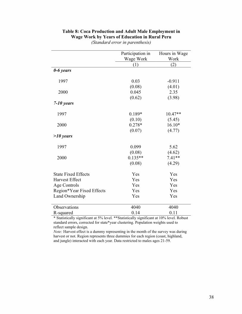
return (Edmonds, Pavcnik, and Topalova 2007). In this context, table 8 shows the effects of the
policies on participation in wage work and weekly hours in wage work of adult males (ages 21 to
59) divided by groups of completed years of education. The idea is to check whether the
interaction of the growing states*post-year is larger for adult males with low education relative
to higher-educated adult males. If anti-coca policies affect returns to education negatively, it is
expected to observe increases in low-skill employment relative to high-skill employment. Results
23
suggest that adult employment changes are consistent with increasing returns to education, rather
than decreasing. Table 8 shows that anti-coca policies are associated with increases in
participation (column 1) and hours worked (column 2) in wage work for men with more than
primary education (more than 7 years of schooling) with small effects on participation and hours
in wage work for men with primary or less.22
Other possible mechanism is related to changes in labor demand. Wages and employment
could decrease in states that are more exposed to coca production. Alternatively, farmers might
shift toward less skill-intensive crops where the demand for child labor increases. Even if
children are not directly involved in the coca economy, a reduction in coca production might
affect other low-skill types of jobs. Several pieces of evidence suggest that children are not
working as substitutes for unskilled labor. As table 9 shows, adult males are more likely to work
in wage work, less likely in agriculture and self-employment. The increase in adult wage work is
explained by increases in employment of male adults with more than primary school with small
effect on participation for men with less than primary school (table 8).
The increase in market and domestic work appears as children filling in for working
parents in the family enterprise and household. The data shows that the increase in market work
for children is not caused by increased in wage work, but it is operating through increases in
agricultural work where 96 percent of children are non-remunerated workers in the family farm
(table 3). The data also shows increases in domestic work (both participation and hours),
especially for girls (table 3). Unreported regression shows declines associated with changes in
coca production in domestic work among adults.
22 An alternative approach to studying the link between returns no schooling and child labor is to look at improvements in school quality. While it is not possible to test directly changes in the number of primary schools and pupil/teacher ratio, evidence suggest that quality didn’t decrease over time. Over the 1990s substantial policy attention has been oriented toward increasing public expenditures on education infrastructure targeted at poor districts with positive effects on school attendance (Paxson and Schady 2002).
24
Finally, critics of drug interdiction and eradication argue that these policies have
substantial welfare effects on rural producers. If the reduction in coca production is associated
with increases in poverty, child labor could increase in coca-growing states relative to non-
growing states. Unreported regressions show that real expenditures fall 2.8 percent in 1997 and
2000 in coca-growing states, respectively (albeit insignificant).23 Lower living standards may
force households to pull children out of school if children are needed in the family farm or
enterprise. The data shows that changes in coca production lead to an increase in the probability
of engaging in market work and hours worked among poorer and middle-income children, with
negative effects on schooling, while richer children were not affected (Table 6).
In addition, the fact that negative schooling results are in non-agricultural households
with no increases in market work (Table 6) might reflect that children living in non-agricultural
households can not work in the family enterprise or farm to buffer the negative shock in adult
labor demand, so the household takes a larger hit to its consumption.24 Table 10 shows falls in
consumption in non-agricultural and agricultural households in both years. The effect is higher
and significant in non-agricultural households where per capita expenditures decreased by 16 and
18 percent in 1997 and 2000, respectively. The results also show that there is a rising in idleness
(children reporting neither working nor attending school) and reduction in school expenditures in
non-farm households located in coca-growing states (albeit insignificant).25 The decline in
schooling in non-farm households might suggest that households may pull children out of school
23 There are no significant changes in other correlates of poverty as well (fertility, idleness of children, housing stock attributes –water, sewage, and electricity-, and durable goods ownership –ratio, TV, and refrigerator). Results are available upon request. 24 One concern might be that the estimate could capture the fact that non-agricultural households are wealthier; however, there is no strong correlation between household expenditure in 1994 and non-agricultural households (the coefficient of correlation is 0.14). 25 The 1997 and 2000 questionnaires are more detailed than the 1994 questionnaire in its inquiries about amount spend in education. The 1994 ask how much the household spend last enrollment, while the 1997 and 2000 ask how much the household spend last time, in which month, and how many times in the last 12 months. As a result, these findings will be interpreted with caution.
25
to save on schooling costs. Saavedra and Suarez (2002) show that even though public education
is free most households finance an important part of the direct cost (books, uniforms,
transportation cost, food, and monetary transfers) as a result of low public spending in basic
education in the country. They estimate that households support about 33 percent of the total
expenditure in primary and secondary education. Similarly, a report about children living in two
coca-growing valleys in Peru found that 34 percent of dropout children do not attend school due
to monetary constraints (UNICEF 2006).
VII. SUMMARY AND CONCLUSIONS
This paper exploits an exogenous shift in coca production from Peru to Colombia in the
mid-1990s to provide empirical evidence on the indirect effects of changes coca production on
child labor and schooling in rural Peru. The main results in this paper suggest that child labor
increased by 18 and 40 percent in coca-growing states in 1997 and 2000, respectively. Not only
the probability of market work increased, but work hours and domestic work as well. Domestic
work increased with higher effects for girls: it increased by 28 percent for girls and 13 percent
for boys in coca-growing states in 2000. Hours worked by both girls and boys increased by 2.5
and 2.0 hours in 1997 and 2000, respectively. Including hours worked engaged in market work
and doing household chores, the estimates suggest children in coca-growing states spent 4.5 and
3.6 more hours a week working in 1997 and 2000. A range of evidence support these results i)
results are robust to the inclusion of household characteristics and state fixed effects, ii)
differences in effects by urban/rural status are also consistent with the notion that anti-coca
policies affect rural households, iii) there are differential effects by whether the child resides in
agricultural or non-agricultural households, and by education of the head of household. Given
26
high school enrollment rates in rural Peru, these results indicate that children are not withdrawn
from school completely but rather working part time.
In addition, adults have less employment probability and work less hours in agricultural
activities. Patterns observed here suggest that children are not working in the formal market as
substitutes for unskilled labor; rather the increase in market and domestic work appears as
children filling in for working parents. In addition, schooling cost appears to play a role in
households where children cannot work in the family enterprise or farm to buffer the negative
shock in adult labor demand.
Overall, these results provide evidence of an undocumented negative effect of anti-coca
policies on household behavior. This complements evidence from other countries, Angrist and
Kugler (2005) in their study on Colombia found that an increased in coca production increased
hours worked by teenage boys but had no effect on employment participation. It is important to
note that the area under coca cultivation in Peru increased in 2004 to 50,300 hectares, the highest
level since 1998 (UNODC 2006). The anti-coca policies imposed in 1995 did not end the drug
war in the Andes.
27
VIII. REFERENCES
Angrist, J., Kugler, A., 2005. Rural Windfall or a New Resource Curse? Coca, Income, and Civil Conflict in Colombia. NBER Working Paper 11219, March. Cambridge MA: National Bureau of Economic Research.
Baland, J., Robinson J., 2000. Is Child Labor Inefficient? Journal of Political Economy. 108(4): 663-679
Basu, K., 1999. Child Labor: Cause, Consequence, and Cure, with Remarks on International Labor Standards. The Journal of Economic Literature. XXXVII, 1083 - 1119.
Basu, K., Hoang Van, P., 1998. The Economics of Child Labor. The American Economic Review 88, 412--427.
Basu, K., Tzannatos, Z., 2003. The Global Child Labor Problem: What do We Know and What We Can Do? World Bank Economic Review. Vol 17.
Bedoya, E., 2003. Las Estrategias Productivas y el Riesgo Entre los Cocaleros Del Valle de los Ríos Apurímac y Ene. in: Aramburu, C., Bedoya, E. (Eds), Amazonia: Procesos Demograficos y Ambientales. CIES. Lima, Peru
Beegle, K., Dehejia, R., Gatti, G., 2006. Child Labor and Agricultural Shocks. Journal of Development Economics. 81: 80-96.
Bhalotra, S. 2000. Is Child Work Necessary? Discussion Paper No 26. London School of Economics.
Bhalotra, S., Tzannatos, Z., 2003. Child Labor: What have we Learnt? Social Protection Discussion Paper, No 317, The World Bank.
Brown, D., Deardoff, A., Stern, R., 2001. Child Labor: Theory, Evidence, and Policy. University of Michigan. Discussion Paper No 474
Cotler, J., 1999. Drogas y Politica en el Peru. La Conexion Norteamericana. Lima: Instituto de Estudios Peruanos.
Duflo, E., 2001. Consequences of School Construction in Indonesia. American Economic Review. 91,795-813.
Duryea, S., Lam, D., Levison. D., 2007. Effects of Economic Shocks on Children’s Employment and Schooling in Brazil. Journal of Development Economics. Forthcoming
Edmonds, E., Pavnick, N., 2005a. Child Labor in the Global Economy. Journal of Economic Perspectives. 19, 199-220
__________________________,2005b. The Effect of Trade Liberalization on Child Labor. Journal of International Economics. 65, 401-419
Edmonds, E., Pavcnik, N., Topalova, P. 2007. Trade Adjustment and Human Capital Investments: Evidence from Indian Tariff Reform. NBER Working Paper 12884, February. Cambridge MA: National Bureau of Economic Research.
Edmonds, E. 2007. Child Labor. Handbook of Development Economics. Volume 4, J. Strauss and T. Paul Schultz, eds. Forthcoming.
Ersado, L., 2005. Child Labor and Schooling Decisions in Urban and Rural Areas: Comparative Evidence from Nepal, Peru and Zimbabwe. World Development. 33, 455-480.
Funkhouser, E., 1999. Cyclical Economic Conditions and School Attendance in Costa Rica. Economics of Education Review. 18, 31-50.
Guarcello, L., Mealli, F., Rosati. F., 2003. Household Vulnerability and Child Labor: The Effects of Shocks, Credit Rationing, and Insurance. Understanding Children’s Work, An Inter-Agency Research Cooperation Project (ILO, UNICEF, World Bank Group).

28
Jacoby, H., 1993. Shadow Wages and Peasant Family Labour Supply: An Econometric Application to the Peruvian Sierra. The Review of Economic Studies. 60, 903-921
_________, 1994. Borrowing Constraints and Progress through School: Evidence from Peru. Review of Economics and Statistics 76, 151-60.
Jacoby, H., Skoufias E., 1997. Risk, Financial Markets and Human Capital in a Developing Country. The Review of Economic Studies. 64, 311-335.
Kruger, D., 2004. Child Labor and Schooling during a Coffee Sector Boom: Nicaragua 1993-1998, in Trabajo Infantil: Teoria y Evidencia desde Latinoamerica, Luis F. Lopez Calva ed., Mexico, D.F: Fondo de Cultura Economica de Mexico, Forthcoming
Kruger, D., 2007. The Effects of Coffee Production on Child Labor and Schooling in Rural Brazil. Journal of Development Economics. 82(2):448-463
Levison, D., Moe, K., 1998. Household Work as a Deterrent to Schooling: An Analysis of Adolescent Girls in Peru. The Journal of Developing Areas. 32, 339-356.
Ilahi, N., 2001. Children's Work and Schooling: Does Gender Matter? Evidence from the Peru LSMS. World Bank Policy Research. Working Paper No. 2745
ILO, 2002. Every Child Counts: New Global Estimates on Child Labour. International Labor Organization, Geneva.
INEI, 1996. Peru Compendio Estadistico 1995-96. Instituto Nacional de Estadistica e Informatica, Lima. Peru
____, 2003. Peru Compendio Estadistico 2003. Instituto Nacional de Estadistica e Informatica, Lima. Peru
Morales, E., 1986 Coca and Cocaine Economy and Social Change in the Andes of Peru. Economic Development and Cultural Change. 35, 143-161.
__________, 1989. Cocaine: White Gold Rush in Peru. The University of Arizona Press. Paxson, C., and Schady, N., 2002. The Allocation and Impact of Social Funds: Spending on
School Infrastructure in Peru. World Bank Economic Review. 16(2), 297-319. Patrinos, H., Psacharopoulos, G., 1997. Family Size, Schooling, and Child Labor in Peru – An
Empirical Analysis. Journal of Population Economics. 10, 387-405. Ranjan, P., 2001. Credit Constraints and the Phenomenon of Child Labor. Journal of
Development Economics. 64(1):81-102 Ray, R., 2000. Analysis of Child Labour in Peru and Pakistan: A Comparative Study. Journal of
Population Economics. 13, 3 – 19. Riley, K., 1996. Snow Job? The Efficacy of Source Country Cocaine Policies. RAND. RGSD-
102. Rojas, I., 2005. Peru: Drug Control Policy, Human Rights, and Democracy, in Drugs and
Democracy in Latin America. The Impact of US Policy, Coletta Youngers and Eilleen Rosin ed., Washington D.C: Lynne Rienner Publishers.
Rucci, G., 2003. Macro Shocks and Schooling Decisions: The Case of Argentina. Economics Department, University of California at Los Angeles. Manuscript.
Saavedra, J., Suarez, P., 2002. El Financiamiento de la Educación Pública en el Perú: El Rol de las Familias. GRADE. Documento de trabajo No 38.
Skoufias, E., Parker, S., 2006. Job Loss and Family Adjustments in Work and Schooling during the Mexican Peso Crisis. Journal of Population Economics. 19, 163–181.
Steiner, R., 1998. Colombia’s Income from the Drug Trade. World Development. 26, 1013-1031 Thoumi, F., 2002. Illegal Drugs, Economy, and Society in the Andes. Washington D.C:
Woodrow Wilson Center Press / Johns Hopkins University Press.
29
UNICEF, 2006. Niños en las Zonas Cocaleras. Un Estudio en los Valles de los Ríos Apurímac y Alto Huallaga. Lima, Peru.
UNODC, 1999. Global Illicit Drug Trends. United Nations Office of Drugs and Crime. Vienna _______, 2002. Global Illicit Drug Trends. United Nations Office of Drugs and Crime. Vienna _______, 2006. World Drug Report United Nations Office of Drugs and Crime. Vienna UNDCP, 2002. Peru Annual Coca Cultivation Survey. United Nations Office of Drugs and
Crime - Illicit Crop Monitoring Program. Vienna _______, 2003. Peru Coca Cultivation Survey. United Nations Office of Drugs and Crime -
Illicit Crop Monitoring Program. Vienna World Bank, 2001. Peruvian Education at a Crossroads. Challenges and Opportunities for the
21st Century. The World Bank. Washington DC.

30
Figure 1: Coca Leaf Production in Bolivia, Colombia, and Peru (In Metric Tons)
0
50,000
100,000
150,000
200,000
250,000
300,000
1989 1990 1991 1992 1993 1994 1995 1996 1997 1998 1999 2000 2001
Coc
a Le
af P
rodu
ctio
n in
Met
ric T
ons
Peru Bolivia Colombia
Source: United Nations Office of Drugs and Crime (2003)

31
Table 1: Descriptive Statistics for Rural Children 6-14 and their Households
Pooled 1994 94-97-2000 1994 1997 2000 Coca-
growing Non-
growing Difference
Child Characteristics
Age 9.80 9.84 9.76 9.82 9.790 9.876 -0.086 (2.60) (2.55) (0.13) Gender (1= Male) 0.50 0.48 0.50 0.51 0.484 0.473 0.010 (0.50) (0.50) (0.02) Market Work 0.43 0.38 0.48 0.42 0.414 0.350 0.06* (0.49) (0.48) (0.02) Wage Work 0.02 0.03 0.01 0.02 0.017 0.029 -0.013 (0.01) (0.01) (0.02) Non-wage work 0.41 0.35 0.47 0.40 0.398 0.321 0.077 (0.03) (0.06) (0.07) Agricultural Work 0.39 0.351 0.437 0.36 0.396 0.320 0.08 (0.03) (0.07) (0.08) Domestic Work 0.63 0.63 0.63 0.61 0.597 0.655 -0.058 (0.07) (0.03) (0.08) School Enrollment 0.94 0.92 0.94 0.97 0.925 0.908 0.017 (0.26) (0.29) (0.01) Years of Schooling 3.22 3.14 3.14 3.35 3.076 3.187 -0.110 (2.28) (2.24) (0.11)
Hours Market Worked 6.42 6.16 6.88 6.18 6.268 6.091 0.177 (10.66) (11.43) (0.54)
Hours Domestic Work 7.15 8.55 6.92 6.33 10.330 10.479 -0.149 (9.85) (10.58) (0.50)
Household Characteristics Age 43.27 43.71 42.67 43.51 42.413 44.628 -2.214* (10.34) (11.42) (0.54) Years of Education 6.09 6.10 5.88 6.30 6.046 6.133 -0.087 (2.72) (3.21) (0.16) Land Ownership 0.64 0.66 0.64 0.62 0.638 0.677 -0.039 (0.48) (0.47) (0.02)
N 5450 1739 1925 1786 * Statistically significant at 5% level. **Statistically significant at 10% level Robust standard errors, corrected for state*year clustering. Population weights used to reflect sample design. Source: 1994, 1997 and 2000 PLSMS

32
Table 2: Child Labor and Coca Production in Rural Peru (Standard error in parenthesis)
(1) (2) (3) (4) 1997 0.090 0.115* 0.022 0.036 (0.06) (0.06) (0.06) (0.06) 2000 -0.025 -0.051 -0.032 -0.018 (0.05) (0.05) (0.07) (0.07) Coca*1997 0.066 0.073 0.025 0.018 (0.08) (0.08) (0.07) (0.07) Coca*2000 0.148* 0.134 * 0.135* 0.123** (0.07) (0.07) (0.07) (0.07) State Fixed Effects Yes Yes Yes Yes Harvest Effect No Yes Yes Yes Age Effect No Yes Yes Yes Region*Year Fixed Effects No No Yes Yes Head of HH Characteristics No No No Yes Land Ownership No No No Yes Observations 5450 5450 5450 5450 R-squared 0.09 0.17 0.19 0.19 * Statistically significant at 5% level. **Statistically significant at 10% level. Robust standard errors, corrected for state*year clustering. Population weights used to reflect sample design. Note: Child labor refers to children engaged in market work (it includes wage employment, self-employment, agriculture, unpaid work in a family business, helping in the family farm, among others). Harvest effect is a dummy representing in the month of the survey was during harvest or not. Region represents three dummies for each region (coast, highland and jungle) interacted with each year. Head of household characteristics are age and education.
33
Table 3: Child Labor and Coca Production in Rural Peru by Type of Work (Standard error in parenthesis)
Agriculture Work Wage Work Domestic Work Any work
(including domestic work) All Boys Girls All Boys Girls All Boys Girls All Boys Girls (1) (2) (3) (4) (5) (6) (7) (8) (9) (10) (11) (12) 1997 0.040 -0.040 0.098** -0.015 -0.023 -0.012 0.009 0.008 0.001 0.024 0.023 0.009 (0.06) (0.07) (0.05) (0.01) (0.02) (0.01) (0.07) (0.10) (0.08) (0.07) (0.09) (0.07) 2000 -0.016 -0.093 0.052 -0.004 -0.012 0.000 0.028 0.034 0.026 -0.011 -0.017 -0.005 (0.06) (0.07) (0.06) (0.01) (0.02) (0.01) (0.07) (0.09) (0.07) (0.08) (0.10) (0.08 Coca*1997 0.016 0.034 0.015 0.007 0.014 0.001 0.076 0.035 0.123 0.040 0.008 0.074) (0.07) (0.08) (0.07) (0.01) (0.02) (0.01) (0.08) (0.09) (0.08) (0.07) (0.08) (0.07 Coca*2000 0.137* 0.128* 0.155* 0.008 0.025 -0.010 0.129 0.069 0.202* 0.118 0.087 0.147* (0.06) (0.07) (0.07) (0.02) (0.02) (0.01) (0.08) (0.10) (0.08) (0.07) (0.08) (0.07) State Fixed Effects Yes Yes Yes Yes Yes Yes Yes Yes Yes Yes Yes Yes Harvest Effect Yes Yes Yes Yes Yes Yes Yes Yes Yes Yes Yes Yes Age-Gender Yes Yes Yes Yes Yes Yes Yes Yes Yes Yes Yes Yes Region*Year Fixed Effects Yes Yes Yes Yes Yes Yes Yes Yes Yes Yes Yes Yes Head of HH Characteristics Yes Yes Yes Yes Yes Yes Yes Yes Yes Yes Yes Yes Land Ownership Yes Yes Yes Yes Yes Yes Yes Yes Yes Yes Yes Yes Observations 5450 2706 2744 5450 2706 2744 5450 2706 2744 5450 2706 2744 R-squared 0.18 0.18 0.19 0.04 0.05 0.01 0.09 0.07 0.08 0.12 0.12 0.11 * Statistically significant at 5% level. **Statistically significant at 10% level. Robust standard errors, corrected for state*year clustering. Population weights used to reflect sample design. Note: Child labor refers to children engaged in market work (includes wage employment, self-employment, agriculture, unpaid work in a family business, helping in the family farm, among others). Harvest effect is a dummy representing in the month of the survey was during harvest or not. Region represents three dummies for each region (coast, highland, and jungle) interacted with each year. Head of household characteristics are age and education.
34
Table 4: Hours Worked and Coca Production in Rural Peru (Standard error in parenthesis)
Market Work Domestic Work Domestic
+ Market Work All Boys Girls All Boys Girls All Boys Girls (1) (2) (3) (4) (5) (6) (7) (8) (9) 1997 -0.663 -1.939 0.026 -1.189 -0.930 -1.572 -1.833 -2.780 -1.588 (0.91) (1.33) (0.77) (1.14) (1.72) (1.22) (1.41) (2.46) (1.40) 2000 -0.647 -1.842 0.290 0.173 1.458 -1.053 -0.464 -0.315 -0.803 (1.36) (2.01) (0.86) (1.56) (2.81) (1.35) (2.15) (3.36) (1.89) Coca*1997 2.566** 3.113** 2.365* 1.900 2.013** 1.670 4.459* 5.127* 4.007** (1.50) (1.92) (1.38) (1.27) (1.14) (1.56) (1.93) (2.02) (2.15) Coca*2000 2.044 2.852* 1.306 1.602 1.246 2.073 3.626** 4.098* 3.326 (1.45) (1.47) (1.69) (1.40) (1.11) (1.95) (2.06) (1.80) (2.56) State Fixed Effects Yes Yes Yes Yes Yes Yes Yes Yes Yes Harvest Effect Yes Yes Yes Yes Yes Yes Yes Yes Yes Age-Gender Yes Yes Yes Yes Yes Yes Yes Yes Yes Region*Year Fixed Effects Yes Yes Yes Yes Yes Yes Yes Yes Yes Head of HH Characteristics Yes Yes Yes Yes Yes Yes Yes Yes Yes Land Ownership Yes Yes Yes Yes Yes Yes Yes Yes Yes Observations 5450 2706 2744 5444 2704 2740 5444 2704 2740 R-squared 0.15 0.16 0.15 0.10 0.05 0.11 0.16 0.15 0.18 * Statistically significant at 5% level. **Statistically significant at 10% level. Robust standard errors, corrected for state*year clustering. Population weights used to reflect sample design. Note: Harvest effect is a dummy representing in the month of the survey was during harvest or not. Region represents three dummies for each region (coast, highland, and jungle) interacted with each year. Head of household characteristics are age and education.

35
Table 5: Schooling and Coca Production in Rural Peru (Standard error in parenthesis)
Attendance Rates Highest Level Attained Over-age a All Boys Girls All Boys Girls All Boys Girls (1) (2) (3) (4) (5) (6) (7) (8) (9) 1997 0.044 0.024 0.063* 0.238* 0.315* 0.164 -0.040 -0.074 -0.007 (0.02) (0.03) (0.03) (0.10) (0.13) (0.13) (0.04) (0.06) (0.04) 2000 0.039 0.049 0.028 0.315* 0.390 0.260** -0.112* -0.167* -0.066* (0.02) (0.03) (0.03) (0.11) (0.14) (0.16) (0.03) (0.04) (0.03) Coca*1997 -0.028** -0.041* -0.014 0.027 0.033 0.039 0.026 0.008 0.040 (0.02) (0.02) (0.02) (0.11) (0.13) (0.12) (0.04) (0.04) (0.05) Coca*2000 -0.020 -0.028** -0.012 -0.011 -0.040 0.025 0.009 -0.005 0.029 (0.02) (0.02) (0.02) (0.11) (0.12) (0.12) (0.04) (0.04) (0.05) State Fixed Effects Yes Yes Yes Yes Yes Yes Yes Yes Yes Harvest Effect Yes Yes Yes Yes Yes Yes Yes Yes Yes Age-Gender Yes Yes Yes Yes Yes Yes Yes Yes Yes Region*Year Fixed Effects Yes Yes Yes Yes Yes Yes Yes Yes Yes Head of HH Characteristics Yes Yes Yes Yes Yes Yes Yes Yes Yes Land Ownership Yes Yes Yes Yes Yes Yes Yes Yes Yes Observations 5450 2706 2744 5389 2673 2716 5450 2706 2744 R-squared 0.06 0.05 0.07 0.71 0.72 0.70 0.24 0.26 0.22 a Over-age is defined as SAGE= [years of education/(age-6)]*100, and =100 for children aged 6 and currently attending school. Over-age equals one if SAGE<100 and 0 otherwise. * Statistically significant at 5% level. **Statistically significant at 10% level. Robust standard errors, corrected for state*year clustering. Population weights used to reflect sample design. Note: Harvest effect is a dummy representing in the month of the survey was during harvest or not. Region represents three dummies for each region (coast, highland, and jungle) interacted with each year. Head of household characteristics are age and education.

36
Table 6: Changes in Child Labor and Schooling, Coca and Non-Coca growing areas
(Standard error in parenthesis)
Panel A: By Location 1997 2000 Urban Rural Urban Rural Market Work -0.003 0.022 0.012 0.132** (0.05) (0.08) (0.05) (0.08) Market Work Hours 0.643 2.638** 0.779 2.112 (0.69) (1.55) (0.78) (1.49) Domestic Work Hours -1.087 2.117 -1.493 1.630 (1.33) (1.40) (1.63) (1.56) Schooling -0.032* -0.026 -0.003 -0.018 (0.02) (0.02) (0.02) (0.02) Panel B: By Parental 1997 2000 Occupation in Rural Areas Agricultural
Households Non-Agricultural
Households Agricultural
Households Non-Agricultural
Households Market Work 0.028 0.037 0.169* 0.005 (0.08) (0.10) (0.08) (0.10) Market Work Hours 2.742 3.006** 2.881 -0.009 (1.72) (1.86) (1.80) (1.71) Domestic Work Hours 2.989* -1.963 1.924 0.125 (1.40) (1.82) (1.42) (2.40) Schooling -0.030 -0.042** -0.012 -0.062*
(0.02) (0.02) (0.02) (0.02)
Panel C: By Parental 1997 2000 Education in Rural Areas Low
Education Middle
Education High
Education Low
Education Middle
Education High
Education Market Work 0.027 0.155 -0.771 0.167* 0.184* -0.03 (0.09) (0.10) (0.09) (0.08) (0.10) (0.09) Market Work Hours 2.818 3.178 0.929 2.812** 1.622 0.507 (1.75) (2.06) (1.99) (1.71) (2.33) (1.95) Domestic Work Hours 1.023 5.445* 3.097 0.702 5.700* 1.269 (1.31) (2.11) (2.25) (1.49) (2.52) (2.58) Schooling -0.037** 0.027 -0.021 -0.009 -0.043** -0.036
(0.02) (0.04) (0.04) (0.02) (0.03) (0.04)
* Statistically significant at 5% level. **Statistically significant at 10% level. Robust standard errors, corrected for state*year clustering. Population weights used to reflect sample design. Note: Child labor refers to children engaged in market work (it includes wage employment, self-employment, agriculture, unpaid work in a family business, helping in the family farm, among others). Regression includes state fixed effects, indicator variables for gender and age of the child; an indicator variable representing in the month of the survey was during harvest or not; three dummies for each region (coast, highland and jungle) interacted with each year; head of household characteristics (age and education).

37
Table 7: Child Labor and Coca Production in Rural Peru: Sensitivity Analysis (Standard error in parenthesis)
Excluding
coast % Poor
< Median % Poor
> Median Low
Population Density
< Median
High Population
Density >Median
Without Migrants
(1) (2) (3) (4) (5) (6) 1997 0.151* 0.227* 0.158 0.153 -0.029 0.027 (0.07) (0.12) (0.14) (0.16) (0.07) (0.06) 2000 -0.035 -0.151 0.190 0.008 -0.069 -0.015 (0.06) (0.10) (0.12) (0.07) (0.07) (0.07) Coca*1997 0.026 0.002 0.067 0.165 -0.049 0.055 (0.08) (0.12) (0.08) (0.12) (0.08) (0.08) Coca*2000 0.114 0.080 0.176* 0.322* -0.007 0.171* (0.08) (0.10) (0.08) (0.11) (0.08) (0.08) State Fixed Effects Yes Yes Yes Yes Yes Yes Harvest Effect Yes Yes Yes Yes Yes Yes Age-Gender Yes Yes Yes Yes Yes Yes Region*Year Fixed Effects No Yes Yes Yes Yes Yes Head of Household Characteristics Yes Yes Yes Yes Yes Yes Land Ownership Yes Yes Yes Yes Yes Yes Observations 4294 2557 2893 2690 2760 4677 R-squared 0.16 0.20 0.21 0.25 0.19 0.20 * Statistically significant at 5% level. **Statistically significant at 10% level. Robust standard errors, corrected for state*year clustering. Population weights used to reflect sample design. Note: Child labor refers to children engaged in market work (it includes wage employment, self-employment, agriculture, unpaid work in a family business, helping in the family farm, among others). Harvest effect is a dummy representing in the month of the survey was during harvest or not. Region represents three dummies for each region (coast, highland, and jungle) interacted with each year. Head of household characteristics are age and education. Population density and percentage of poor people refers to the district of residency, this data comes from the 1993 Peruvian Census.
38
Table 8: Coca Production and Adult Male Employment in Wage Work by Years of Education in Rural Peru
(Standard error in parenthesis)
Participation in Wage Work
Hours in Wage Work
(1) (2) 0-6 years 1997 0.03 -0.911 (0.08) (4.01) 2000 0.045 2.35 (0.62) (3.98) 7-10 years 1997 0.189* 10.47** (0.10) (5.45) 2000 0.278* 16.10* (0.07) (4.77) >10 years 1997 0.099 5.62 (0.08) (4.62) 2000 0.135** 7.41** (0.08) (4.29) State Fixed Effects Yes Yes Harvest Effect Yes Yes Age Controls Yes Yes Region*Year Fixed Effects Yes Yes Land Ownership Yes Yes Observations 4040 4040 R-squared 0.14 0.11 * Statistically significant at 5% level. **Statistically significant at 10% level. Robust standard errors, corrected for state*year clustering. Population weights used to reflect sample design. Note: Harvest effect is a dummy representing in the month of the survey was during harvest or not. Region represents three dummies for each region (coast, highland, and jungle) interacted with each year. Data restricted to males ages 21-59.
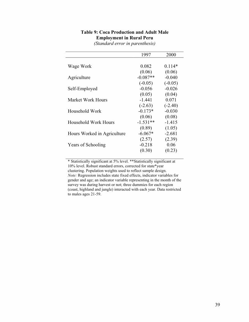
39
Table 9: Coca Production and Adult Male Employment in Rural Peru
(Standard error in parenthesis)
1997 2000 Wage Work 0.082 0.114* (0.06) (0.06) Agriculture -0.087** -0.040 (-0.05) (-0.05) Self-Employed -0.056 -0.026 (0.05) (0.04) Market Work Hours -1.441 0.071 (-2.63) (-2.40) Household Work -0.173* -0.030 (0.06) (0.08) Household Work Hours -1.531** -1.415 (0.89) (1.05) Hours Worked in Agriculture -6.067* -2.681 (2.57) (2.39) Years of Schooling -0.218 0.06 (0.30) (0.23) * Statistically significant at 5% level. **Statistically significant at 10% level. Robust standard errors, corrected for state*year clustering. Population weights used to reflect sample design. Note: Regression includes state fixed effects, indicator variables for gender and age; an indicator variable representing in the month of the survey was during harvest or not; three dummies for each region (coast, highland and jungle) interacted with each year. Data restricted to males ages 21-59.
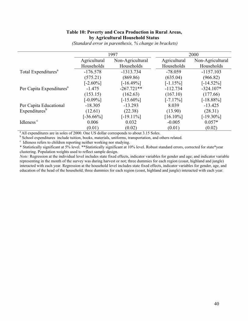
40
Table 10: Poverty and Coca Production in Rural Areas, by Agricultural Household Status
(Standard error in parenthesis, % change in brackets)
1997 2000 Agricultural
Households Non-Agricultural
Households Agricultural Households
Non-Agricultural Households
Total Expendituresa -176.578 -1313.734 -78.059 -1157.103 (575.21) (869.86) (635.04) (966.82) [-2.60%] [-16.49%] [-1.15%] [-14.52%] Per Capita Expendituresa -1.475 -267.721** -112.734 -324.107* (153.15) (162.63) (167.10) (177.66) [-0.09%] [-15.60%] [-7.17%] [-18.88%] Per Capita Educational -18.305 -13.293 8.039 -13.425 Expendituresb (12.61) (22.38) (13.90) (28.31)
[-36.66%] [-19.11%] [16.10%] [-19.30%] Idleness c 0.006 0.032 -0.005 0.057* (0.01) (0.02) (0.01) (0.02) a All expenditures are in soles of 2000. One US dollar corresponds to about 3.15 Soles. b School expenditures include tuition, books, materials, uniforms, transportation, and others related. c Idleness refers to children reporting neither working nor studying. * Statistically significant at 5% level. **Statistically significant at 10% level. Robust standard errors, corrected for state*year clustering. Population weights used to reflect sample design. Note: Regression at the individual level includes state fixed effects, indicator variables for gender and age; and indicator variable representing in the month of the survey was during harvest or not; three dummies for each region (coast, highland and jungle) interacted with each year. Regression at the household level includes state fixed effects, indicator variables for gender, age, and education of the head of the household; three dummies for each region (coast, highland and jungle) interacted with each year.