Labor Market Search and Schooling Investment

Christopher FlinnJoseph Mullins

No. 295March 2013

www.carloalberto.org/research/working-papers

© 2013 by Christopher Flinn and Joseph Mullins. Any opinions expressed here are those of the authorsand not those of the Collegio Carlo Alberto.

ISSN 2279-9362

Labor Market Search and Schooling Investment1

Christopher Flinn

Department of Economics

New York University

Collegio Carlo Alberto

Moncalieri, Italy

Joseph Mullins

Department of Economics

New York University

First Draft: June 2010

This Draft: February 2013

Keywords: Labor market search; schooling choice; hold-up; Nash bargaining.

JEL Classifications: J24, J3, J64

1The C.V. Starr Center for Applied Economics at New York University has partially funded thisresearch. James Mabli greatly aided in the development of the modeling strategy. We are gratefulto Cristian Bartolucci for many useful comments and discussions, as well as to Fabien Postel-Vinayfor a stimulating (formal) discussion of the paper at the SOLE Meetings in London, June 2010,and to participants in the Milton Friedman Institute Conference in honor of James Heckman heldin Chicago, November 2010. We are responsible for all errors, omissions, and interpretations.

Abstract

We generalize the standard search, matching, and bargaining framework to allow individ-uals to acquire productivity-enhancing schooling prior to labor market entry. As is well-known, search frictions and weakness in bargaining position contribute to under-investmentfrom an efficiency perspective. In order to evaluate the sensitivity of schooling investmentsto “hold up,” the model is estimated using Current Population Survey data. We focus onthe impact of bargaining power on schooling investment, and find that the effects are largein the partial equilibrium version of the model. However, large increases in bargainingpower in the general equilibrium version of the model choke off firm vacancy creation andactually reduce the level of schooling investment.

1 Introduction

A large number of papers, both theoretical and applied, have examined labor marketphenomena within the search and matching framework, with some embedded in a simplegeneral equilibrium setting.1 Virtually all of the empirical work performed using thisframework has assumed that individual heterogeneity is exogenously determined at thetime of entry into the labor market. Perhaps the most important observable correlate ofsuccess in the labor market is schooling attainment. In this paper we extend the standardsearch and matching framework to allow for endogenous schooling decisions, and obtainestimates of both partial and general equilibrium versions of the model.2

We develop a simple model of schooling investment decisions, where higher levels ofschooling investments are (generally) associated with better labor market environments.Individuals are differentiated in terms of initial ability, a, and the heterogeneity in thischaracteristic, along with the structure of the labor market, is what generates equilibriumschooling distributions. As is standard, we utilize axiomatic Nash bargaining to determinethe division of the surplus between workers and firms. For simplicity, and due to the natureof the data we utilize, we assume that employed individuals do not receive alternative offersof employment, i.e., there is no on-the-job (OTJ) search. We discuss some of the possiblemodifications of our findings that would occur if OTJ search was considered.3

There is a long-standing literature examining the essence of the hold-up problem andthe role contracts play to reduce, or altogether avoid, hold-up (see Malcomson (1997)and Acemoglu (1996,1997) for a number of citations to the relevant literature). At thecore of the problem is the notion that investments must be made before agents meet and,thus, greater market frictions generally lead to more serious hold-up problems. Acemogluand Shimer (1999) examine the potential for hold-up problems in frictional markets andinvestigate the manner in which markets can internalize the resulting externalities. Their

1A large number of macroeconomic labor applications are cited in Pissarides (2000) and the recentsurvey by Shimer et al. (2005). In terms of econometric implementations of the model, examples are Flinnand Heckman (1982), Eckstein and Wolpin (1995), Postel-Vinay and Robin (2002), Dey and Flinn (2005),Cahuc et al (2006), and Flinn (2006).

2There are a number of ambitious empirical papers which estimate life cycle individual decision rulemodels of schooling choice and labor market behavior, such as Keane and Wolpin (1997) and Sullivan(2010). This approach has been extended to allow for the endogenous determination of rental rates forvarious types of human capital, e.g., Heckman et al. (1998), Lee (2005), and Lee and Wolpin (2006). Theseframeworks do not allow investigation of surplus division issues and the hold-up problem since they arebased on a competitive labor market assumption. Eckstein and Wolpin (19995) estimate a search andmatching model for various demographic groups in order to evaluate the “return to schooling” along anumber of dimensions (e.g., contact rates, matching distributions, bargaining power), but do not explicitlyconsider the schooling choice decision.

3Adding on-the-job search alters the details of what constitutes “bargaining power” in the market, butnot the fact that a lack of “generalized” bargaining power, which may include the possibility of renegotiationof contracts as in Postel-Vinay and Robin (2002), Dey and Flinn (2005), and Cahuc et al (2006), willnegatively impact the individual’s incentive to invest in human capital.

1

focus is on identifying ways in which hold-up and inefficiencies can be mitigated in labormarkets characterized by ex-ante worker and firm investments and search frictions and findthat this can be achieved in wage-posting models with directed search.4

The generalized Nash bargaining power parameter has a direct impact on the extent ofthe hold-up problem the worker faces vis-a-vis pre-market schooling investment decisions.While there are a number of estimates of the bargaining power parameter within models ofNash bargaining and matching, the estimates tend to vary significantly with the assump-tions made regarding the presence of on-the-job (OTJ) search, and given OTJ search, thenature of the renegotiation process, as well with respect to the data set used in estimation.In their search, matching, and Nash bargaining frameworks, Dey and Flinn (2005), Cahucet al. (2006), and Flinn and Mabli (2009) found that allowing for OTJ search substantiallyreduced the estimate of the worker’s bargaining power parameter in comparison with thecase in which OTJ search was not introduced (e.g., Flinn 2006). To some degree, this isa result of allowing for Bertrand competition. When competition between firms is intro-duced, substantial wage gains over an employment spell can be generated simply from thisphenomenon, even when the individual possesses little or no bargaining power in terms ofthe bargaining power parameter. Indeed, the (approximately) limiting case of this is thatconsidered by Postel-Vinay and Robin (2002), in which workers possessed no bargainingpower whatsoever. While the hold-up problem would seem to be particularly severe in thiscase, even to the extent that individuals would have no incentive to invest in human capi-tal, this is not the case when Bertrand competition between competing potential employersoccurs, which is when the individual can recoup some of the returns to her pre-market in-vestment. Incentives to invest in their model are directly related to the contact rates withother potential employers in the course of an employment spell, most importantly, as wellas the other rates of event occurrence (i.e., the offer arrival rate in the unemployed stateand the rate of exogenous separation).

As our model structure makes clear, simply estimating separate behavioral models ofthe labor market for different schooling classes is at a minimum inefficient, and, more seri-ously, may lead to misinterpretations of labor market structure. For this reason, wheneverpossible, potentially endogenous individual characteristics acquired before or after entryinto the labor market should be incorporated into the structure of the search, matching, andbargaining framework. In order to do so in a tractable manner requires stringent assump-tions regarding the productivity process, bargaining, etc., as is evident in what follows.Using our simple and tractable model, we are able to make some preliminary judgementsregarding the impact of hold-up on schooling investment. We find that bargaining powerhas a strong impact on the incentive to invest in schooling in the partial equilibrium versionof the model and that the amount of schooling is monotone increasing in bargaining power,as theory leads us to expect. However, in the general equilibrium version of the model,

4It is well-known that wage-posting models have requirements of commitment to mitigate the incentivesof firms to renegotiate contracts with individual workers.

2

large increases in the bargaining power of workers lead to decreases in schooling attainmentand the welfare of workers as firms dramatically reduce the number of vacancies created.In the econometric section, we discuss why it is not possible to estimate the parameters ofthe Mortensen-Pissarides matching function given the data at our disposal. However, ourresults hold for a variety of “reasonable” values of the matching function parameters asreported in the Petrongolo and Pissarides (2001) survey of the empirical literature on theestimation of matching functions using aggregate data.

Our work is closest in spirit to that of Charlot and Decreuse (2005,2010), who performa theoretical analysis of the hold-up problem in a search and matching framework that isa special case of the one considered here. In their model, productivity is solely a functionof individual innate ability and their schooling level, whereas our model allows for matchheterogeneity that we find to be empirically very important.5 The interesting theoreticalpoint that they make is that the schooling decisions of individuals to not lead to efficientoutcomes for the economy since individuals neglect the impact of their schooling decisionon firms’ vacancy creation. As in our model, there is a critical ability level a∗ such that allindividuals with ability a less than a∗do not acquire higher education. When an individualnear the margin goes to school, he lowers the quality level in each schooling sub-market,thereby reducing the incentives for firms to post vacancies in either market. This typeof effect will also exist in our framework, though it will be muted due to the presence ofmatch-specific heterogeneity, the variance of which dominates that of individual ability.

The plan of the paper is as follows. In Section 2, we develop a bargaining model in apartial equilibrium framework, with education decisions made prior to entering the labormarket. Section 3 extends the basic model to allow schooling sub-markets to be character-ized by different vectors of primitive parameters, such as contact and dissolution rates. InSection 4 we analyze the general equilibrium case in which contact rates are determined bythe measure of unemployed searchers and the vacancy creation decisions of firms. In Section5 we describe the sample used to estimate the model and discuss identification of modelparameters and the estimator used. Section 6 presents model estimates and (empirical)comparative statics exercises. Section 7 concludes.

2 Model with Homogeneous Schooling Markets

2.1 Overview

By now there have been a number of models that have been estimated within the search,matching, and bargaining framework (e.g., Postel-Vinay and Robin (2002), Dey and Flinn(2005), Cahuc et al. (2006), and Flinn (2006)). These models posit random matchingbetween workers and firms, at least within observationally differentiated labor markets.

5Our model also differs in that we allow for different values of offer rates, dismissal rates, and bargainingpower across the two schooling markets.

3

The flow (in continuous time) productivity of a match between worker i and firm j isassumed to be given by

yij = aiθij pj, (1)

where ai is individual i′s time- and match-invariant productivity, pj is firm j′s time- andmatch-invariant productivity, and θij is a random match component that is assumed to beindependently and identically distributed (i.i.d.) over all potential (i, j) matches accordingto the distribution function G. Analyses that utilize worker-firm matched data (e.g., Postel-Vinay and Robin (2002) and Cahuc et al. (2006)) typically assume that G is degeneratewith θij = 1 ∀(i, j). Analyses that have used only observations from the supply side of themarket (e.g., Dey and Flinn (2005) and Flinn (2006)) instead assume that ai = 1 ∀ i andpj = 1 ∀ j.

We can think of the specification of flow productivity in (1) terms of the standard linearmodel, and this is particularly clear when we consider the logarithm of the expression

ln yij = ln ai + ln pj + ln θij.

The terms ln ai and ln pj represent “main effects,” in the language of linear models, whileln θij represents a higher-order interaction effect. One common specification of flow pro-ductivity restricts the (logarithmic) model to include only main effects, whereas the otherspecification restricts the model to include no main effects. There is no reason to thinkthat either restriction is entirely appropriate, so that the estimation of a model that poten-tially includes both types of contributions to worker-firm output may produce interestingempirical implications and a more general data generating process.

The main contribution of the paper, however, is to broaden the interpretation of the“main” effects, ai and pj. The nonparametric estimation of the distributions of these is animportant contribution of the Postel-Vinay and Robin (2002) and the Cahuc et al. (2006)analyses. In this paper, we attempt to extend the standard labor market search frameworkto include pre-market investments.6 For empirical tractability, we limit attention to thecase in which workers and firms can decide, prior to entering the market, whether tomake a costly investment that will improve their (idiosyncratic) productivity by somefixed amount. In the case of workers, we assume that the individual first is able to observetheir ability endowment, a. Prior to entering the labor market, the individual can eitherstop their schooling at the mandatory level or continue on to acquire a higher level offormal education. A student of type a who stops schooling at the mandatory level entersthe labor market with idiosyncratic ability ai = aih1, where we adopt the normalizationh1 = 1. If they were to complete an advanced degree program, the individual would enterthe market with ability level ai = aih2, with h2 > h1. Similar possibilities exist on the

6There has been work on the effect of the hold-up problem on pre-marital investments, with a recentcontribution being Chiappori et al. (2009). However, most contributions, such as this one, are primarilytheoretical in nature. To our knowledge, no labor market search model with bargaining that includespre-market investments has been estimated.

4

firm side of the market, so that a firm with a productivity endowment of pj can undertakecostly investment so as to make its productivity pj = pjk2 or can enter the market withoutundertaking productivity-enhancing investment so that pj = pjk1 = pj , where we haveadopted the normalization that k2 > k1 = 1.

In our analysis we examine the role of labor market characteristics, particularly bargain-ing power, on the investment decisions of workers. One of the contributions of the analysisis to demonstrate that when workers and firms are able to invest prior to market entry, thedistributions of worker and firm productivities cannot properly be considered as “primi-tives,” that is, these distributions are responsive to changes in labor market parametersand policy interventions.

2.2 No Firm Heterogeneity

Due to data limitations, we are not able to properly consider the general case of two-sidedinvestment, so that throughout the paper we will assume that firms are homogeneous, i.e.,pj = 1 ∀ j. In this case, the output at a match is given by

y = ahsθ,

where θ is i.i.d. with c.d.f. G, hs is the individual’s (schooling) human capital level, and a isindividual ability, which is a permanent draw from the distribution Fa with correspondingdensity fa. Hereafter we drop the individual and firm subscripts - they are redundant sincea and h refer to individuals and θ is a match value.) As mentioned above, we restrict ourattention to the case of S = 2, where s = 1 corresponds to high school and partial college,roughly, and s = 2 to college completion.7

The analysis, both theoretical and empirical, can be made much more tractable if wemake the following set of assumptions.

1. All parameters describing the labor market are independent of schooling status withthe exception of hs. (This can easily be weakened, which is done in the next section.)

2. The flow value of unemployment to a type a individual with schooling level s is givenby

b(a, s) = b0ahs.

7This classification was determined to some extent empirically. Our original classification schemegrouped together all those sample members who had completed some level of schooling beyond high school.We found that those who had attended college but not completed it were far more similar, in terms of labormarket outcomes, to those with only a high school education than to those who had completed four yearsof college. As a result, we grouped together all those who had not completed at least a four-year collegedegree. Even with this classification, 30 percent of our sample of 25-34 year old males fell into schoolingclass s = 2.

5

This last assumption is similar to that made in Postel-Vinay and Robin (2002) and inBartolucci (2009).

Since we primarily use data from the Current Population Survey, which is a pointsample of the labor market process of household members, we assume no on-the-job (OTJ)search. This assumption is not innocuous for some of the comparative statics exercises weconduct below, and in the conclusion of the paper we discuss how allowing OTJ searchcould affect our results.

We begin by considering the case in which, across schooling “sub-markets,” all jobsearch environments are identical (i.e., they have identical parameters α1 = α2, η1 = η2,etc.). In this case, the value of search to an individual of type (a, hs) who is entering thelabor market as an unemployed searcher, can be summarized solely in terms of the producta ≡ ahs, and the value of unemployed search to such an individual is given by VU (a). Interms of the Nash bargaining problem, the worker-firm pair solves

maxw

(VE(w, a)− VU(a))αVF (w, θ)

1−α,

where

VE(w, a) =w + ηVU (a)

ρ+ η

VF (w, θ, a) =θa− w

ρ+ η.

Note that we have assumed that the firm’s outside option under Nash bargaining is equalto 0, which is consistent with the common free entry condition that drives the value of anunfilled vacancy to 0.8 The solution to the Nash bargaining problem yields

w(θ, a) = αθa+ (1− α)ρVU (a),

and sinceρVU (a) ≡ y∗(a) = aθ∗(a),

we havew = a(αθ + (1− α)θ∗(a)). (2)

In terms of the value of unemployed search given a, we have

ρVU (a) = b0a+ λ

∫

θ∗(a)(VE(a, θ)− VU (a))dG(θ)

⇒ aθ∗(a) = b0a+λαa

ρ+ η

∫

θ∗(a)(θ − θ∗(a))dG(θ). (3)

8This assumption is utilized below when we generalize the model to allow for endogenous vacancycreation by firms.

6

Since this last equation is independent of a, we have

θ∗(a) = θ∗ for all a,

which means that the reservation output value for an individual of ability a with schoolinglevel s is simply

y∗(a, s) = ahsθ∗. (4)

This result makes the consideration of the schooling choice problem straightforward.When an individual of type a has schooling level s and enters the labor market, the expectedvalue of the labor market career is given by VU (ahs). Then for a type a individual, thevalue of schooling level s at the time of entry into the labor market is

VU (ahs) = ρ−1ahsθ∗.

We consider schooling level 1 as the baseline, that is, it is the required level of schooling forall individuals. To complete schooling level 2, instead, a total cost of c must be incurred,that is assumed to be the same for all individuals. Individuals base their decision tocomplete schooling level 2 on the comparison between the values of entering the labormarket with human capital h2 or h1. Then an individual with ability level a will attendschool if

ρ−1ah2θ∗ − ρ−1ah1θ

∗ > c

⇒ a >ρc

(h2 − h1)θ∗.

Then, given that c > 0 and θ∗ > 0, there exists a critical value a∗ defined as

a∗ =ρc

(h2 − h1)θ∗,

with an individual of type a ≥ a∗ acquiring schooling and a person a < a∗ not acquiringfurther schooling.9 In the empirical analysis conducted below, we assume that the support

9In an earlier version of the paper, we explicitly accounted for the difference in labor market entry datesunder the two schooling options as part of the model. In such a case, with instantaneous cost c, the totaldiscounted value of continuing in higher education is exp(−ρτ )ρ−1ah2θ

∗, where τ is the length of timerequired to complete advanced schooling. The total cost absorbed over the schooling period is

c = ρ−1

c(1− exp(−ρτ )).

Then the individual acquires schooling level 2 if

exp(−ρτ )ρ−1ah2θ

∗ − ρ−1

ah1θ∗

> c,

and the condition for schooling to be acquired by any a when c > 0 is that exp(−ρτ )h2 − 1 > 0. Giventhat ρ and τ are fixed in our analysis, this puts a strong restriction on the estimate of h2 for their tobe a critical value rule of the type we describe when explicitly considering discounting phenemona. Wenote that Cherlot and Decreuse (2005,2010) also ignore discounting when comparing the values of the twoschooling choices in their theoretical analysis of schooling investment in the presence of search frictions andbargaining.

7

of the distribution of a is R+, so that the proportion of individuals in the population whoacquire schooling is given by 1− Fa(a

∗) > 0.

2.3 Comparative Statics Results

Given the simplicity of the decision rule, comparative statics results are easily derived. Forthe most part, they are intuitively reasonable, which is a strength of this modeling setup.

The focus of the paper is schooling decisions. In our two schooling class model, we cansummarize the schooling distribution in terms of the probability that a population membergraduates from college, the likelihood of which is

P2 ≡ P (s = 2) = Fa(a∗),

where Fa denotes the survivor function associated with the random variable a. The resultsare:

1. ∂P2/∂c < 0. The proportion of the population attending college is decreasing in thedirect costs of college attendance.

2. ∂P2/∂h2 > 0. This is perhaps the most intuitive result. The greater the impacton labor market productivity, the greater the number of individuals who completecollege.

3. ∂P2/∂θ∗ > 0. Now θ∗ is not a primitive parameter of course, but most primitive

parameters characterizing the labor market only affect the schooling decision throughθ∗, which is a determinant of the value of search for all agents (recall that the criticaloutput level for job acceptance is ahsθ

∗). Through this value, we can determine theimpact of the most of the various labor market parameters on the schooling decision.

(a) ∂P2/∂λ > 0. An increase in the arrival rate of offers increases θ∗, and henceincreases the value of having a higher productivity distribution.

(b) ∂P2/∂η < 0. An Increase in the (exogenous) separation rate decreases θ∗ andhence decreases the value of becoming more productive when matched with anemployer.

The main comparative statics result, which is the focus of the paper, concerns the effectof bargaining power α on schooling. While the result is obvious at this point, we state itmore formally than the other results.

Proposition 1 Increases in bargaining power on the workers’ side of the market result in

increases in schooling level, or∂P2

∂α> 0.

8

We should note that this result is only true for the case in which the contact ratesbetween searchers and firms are held fixed, i.e., only in partial equilibrium. As we willsee below, this result will not in general be true in the general equilibrium version of themodel.

2.4 Empirical Implications

Here we consider the model’s implications for the labor market outcomes of individualsin the two schooling classes. In particular, we look at unemployment rates and wagedistributions for the two schooling classes.

2.4.1 Unemployment Experiences

Under our modeling assumptions, the steady state unemployment rate for an individualof type a is independent of a. This is due to the fact that the likelihood that any jobis acceptable to an individual of type a is simply G(θ∗), which is independent of a. Theproportion of time an individual of type a spends in unemployment, or the steady stateprobability that they will occupy the unemployment state, is simply

P (U |a) =η

η + λG(θ∗)= P (U).

Thus, the assumption that the primitive parameters are identical across schooling groupsproduces the implication that there is no difference in unemployment experiences acrossschooling groups.

2.4.2 Wage Distributions

We assume that the support of the matching distribution G is the nonnegative real line,and that G is everywhere differentiable on its support with corresponding density g. Wehave established that the schooling continuation set is defined by [a∗,∞). Now, from (2)we know that

θ =wa− (1− α)θ∗

α,

where the lower limit of the wage distribution for an individual of type a is w(a) = aθ∗.Then the cumulative distribution function of wages for a type a individual is

Fw(w|a) =G(α−1(w

a− (1− α)θ∗))−G(θ∗)

G(θ∗), w ≥ aθ∗,

and the corresponding conditional wage density is given by

fw(w|a) =1

αa

g(α−1(wa− (1− α)θ∗))

G(θ∗), w ≥ aθ∗.

9

Now we consider the wage densities by schooling class. For this purpose, we write

fw|a,s(w|a, s) =1

αahs

g(α−1( wahs

− (1− α)θ∗))

G(θ∗), w ≥ ahsθ

∗.

Then the marginal density of wages in schooling class s is given by

fw|s(w|s) =1

αhsG(θ∗)

∫

a−1g(α−1(w

ahs− (1− α)θ∗))dF (a|s), w ≥ hsa(s)θ

∗,

where a(s) denotes the lowest ability individual who makes schooling choice s. Given thesimple form of the schooling continuation decision, the density of wages among those witha high school education is

fw|s(w|s = 1) =1

αG(θ∗)

∫ a∗

a

a−1g(α−1(w

a− (1− α)θ∗))

dF (a)

F (a∗), w ≥ aθ∗, (5)

where a is the lowest value of a in the population, while the density of wages among thecollege-educated population is

fw|s(w|s = 2) =1

αh2G(θ∗)

∫ a

a∗a−1g(α−1(

w

ah2− (1− α)θ∗))

dF (a)

F (a∗), w ≥ a∗h2θ

∗. (6)

The conditional wage densities for the two schooling groups differ, then, not only be-cause college education improves the productivity of any individual who acquires it, butalso through the systematic selection induced on the unobserved ability distribution Fa

by the option of going to college. In terms of the conditional (on s) wage distributions,we note that the upper limit of the support of both distributions is ∞. The distributionsdo differ in their lower supports, with this lower bound equal to aθ∗ for those with highschool education and a∗h2θ

∗ for those with college. Since a∗h2 > a, the lower support ofthe distribution of the college wage distribution lies strictly to the right of the high schoolwage distribution.

Proposition 2 The wage distribution of the college educated first order stochastically dom-

inates that of the high school educated.

Proof. Since h2 > h1 = 1, for any a, Fw(w|a, h2) first order stochastically dominatesFw(w|a, h1). For any s, Fw(w|a

′, s) first order stochastically dominates the distributionFw(w|a, s) whenever a′ > a. Since a′ ≥ a∗ > a for all a′ ∈ [a∗, a] and a ∈ [a, a∗), theempirical distributions are strictly ordered in the sense

Fw|1(w|1) ≥ Fw|2(w|2) for all w ≥ aθ∗.

10

From this result, it immediately follows that the average wage is greater among thecollege educated. More importantly, the wages of the college-educated exceed those witha high school education at every quantile of the respective distributions.

Before proceeding to investigate some extensions of the basic model, we present somedescriptive evidence regarding specific empirical implications. The data used in all ofthe empirical analysis below will be described in more detail in the sequel. In terms ofthe general characteristics of the sample, it is drawn from monthly Current PopulationSurvey samples from 2005. We restrict the sample to males between the ages of 25 and34, inclusive. Further details of the sample selection used are provided in section 5.1.The “high schooling” category, corresponding to s = 2, consists of individuals who havecompleted (at least) a four year college program. The “low schooling” category is all others.

Figure 1.a and 1.b contain the plots of the wage distributions by schooling group. Wesee from these figures that the wages of the low schooling group members are highly concen-trated in the range 6 to 20 dollars, while the high schooling group wages show considerablymore dispersion. Figure 1.c displays the distribution of total wages. Approximately 30percent of those in the wage sample have completed college, so that the marginal wagedistribution closely resembles the non-college wage distribution at low values of w. Thisis not the case at high wage levels, where virtually all observations are associated withcollege-completers.

Proposition 3 implies that the high schooling wage distribution first order stochasticallydominates the low schooling wage distribution. Figure 1.d presents evidence regarding thisimplication. The figure plots

F (w(i)|s = 1)− F (w(i)|s = 2)

for an increasing sequence of wages, w(1) < ... < w(K). First order stochastic dominatesimplies that all values in this sequence should be nonnegative, and the figure strongly bearsout this claim.

The homogeneous labor market assumption is not consistent with the observed unem-ployment rate for the two education groups. From Table 1, we note that the unemploymentrate for college-completers is only 2.16%, while among those with less schooling it is 4.67%.A simple adjustment allows the model to produce such an outcome, and we now turn tothis generalization.

3 Separate Schooling Sub-markets

We continue within the partial equilibrium setting of the previous section, but considerrelaxing some of the more restrictive (from an empirical perspective) features of that model.In particular, we know from the large number of structural estimation exercises involvingsearch models that the primitive parameters across sub-markets are often found to bemarkedly different (see, for example, Flinn (2002)). In particular, it is often noted that

11

the unemployment rate differs across schooling groups, with those with lower completedschooling yields often having lengthier and more frequent unemployment spells. As we sawabove, such a result is not consistent with the assumption that all primitive labor marketparameters are the same across schooling classes.

The situation we consider is one in which each schooling class inhabits a sub-labormarket, which has its own market-specific parameters (λs, ηs, αs). The parameter ρ, beinga characteristic of individual agents (individuals and firms), is assumed to be homogeneousacross labor markets, as is the baseline unemployment utility flow parameter, b0. The matchproductivity distribution G is also identical across markets. In terms of the productivityof an individual, nothing has changed from the previous case, since y(a, s, θ) = ahsθ = aθ,so that the distribution of y is a function of the scalar a and the common (to all matches)distribution G. However, it is no longer the case that the critical match value will be thesame across schooling sub-markets. Because primitive parameters differ across markets, ais no longer a sufficient statistic for the value of search of an individual; instead a minimalsufficient statistic is the pair (a, s). This is clear if we reconsider the functional equationdetermining the value of search in the homogeneous sub-markets case, which was given in(3), adapted to the heterogeneous case. Then we have

aθ∗(a, s) = b0a+λsαsa

ρ+ ηs

∫

θ∗(a,s)(θ − θ∗(a, s))dG(θ).

The solution θ∗(a, s) now clearly is independent of a, as before, but is not independentof s. Thus there is a common critical value θ∗(s) shared by all individuals with schoolingchoice s, which is independent of their ability a.

We now turn to the schooling choice decision in this case. The critical match value foran individual of type a in schooling market s is given by ahsθ

∗(s) = aθ∗(s), so that thevalue of unemployed search in this sub-market is given by ρ−1aθ∗(s). Then the net valueof college education to an individual of type a is

ρ−1ah2θ∗(2) − c− ρ−1aθ∗(1),

so that the critical ability level a∗ is given by

a∗ =cρ

h2θ∗2 − θ∗1.

For a∗ to be positive, it is necessary that h2θ∗2 − θ∗1. This condition is satisfied in the

empirical work conducted below.

3.1 Comparative Statics Results

Comparative statics results are fundamentally different in this case in the sense that certainmarket-specific primitive parameters only impact the value of unemployed search within

12

their particular sub-market. By simple extension of the homogeneous results above, theresults regarding ∂P2/∂c < 0 remain the same since the cost structure of acquiring schoolingis identical in the two cases. It is also clearly the case that ∂P2/∂h2 > 0. The maindeparture from the previous case regards the presence of θ∗1 and θ∗2. We note that

1. ∂P2/∂θ∗1 < 0. As before, θ∗1 is not a primitive parameter, but the primitive parameters

specific to sub-market 1 only affect the schooling decision through θ∗1. Then

(a) ∂P2/∂λ1 < 0. Increases in the arrival rate of offers in the low-schooling marketincrease θ∗1, and increase the relative value of a low schooling level.

(b) ∂P2/∂η1 > 0. Such an increase decreases the value of a low schooling level.

2. ∂P2/∂θ∗2 > 0.

(a) ∂P2/∂λ2 > 0

(b) ∂P2/∂η2 < 0

3. Perhaps most interesting is the impact of market-specific bargaining powers αs onthe schooling decision. When there is one bargaining power parameter that holdsthroughout all educational labor markets, the meaning of hold-up is relatively un-ambiguous. When there are market-specific bargaining power parameters, a relativenotion of hold-up is more appropriate. Clearly we have

∂P2

∂α1< 0.

∂P2

∂α2> 0.

It is important to note that α2 could be quite low, and yet a substantial proportionof agents may choose the high schooling level if α1 is significantly lower yet.

3.2 Empirical Implications

There are a few obvious differences in the empirical implications of the homogeneous andheterogeneous labor market models.

3.2.1 Unemployment

The characteristic scalar a is no longer sufficient for describing an individual’s probability oflabor market events, in general, except when a implies a unique value of s. While this maybe the case as long as there exists a unique a∗ that determines the schooling continuationset and h2 > 1, we will condition on both a and s to make the situation a bit more

13

transparent. Now, in general, we will have different steady state unemployment rates forthe two schooling groups, since

P (U |a, s) =ηs

ηs + λsG(θ∗s)= Ps(U), s = 1, 2.

As before, within a schooling group unemployment probabilities are homogeneous. Withoutfurther restrictions on the event rate parameters and the bargaining power parameters, itis not possible to order the unemployment probabilities across schooling sectors.

3.2.2 Wage Distributions

The lower bound on the support of the wage distribution associated with schooling types is now given by w(1) =aθ∗1 for the low schooling group and by w(2) = a∗h2θ

∗2 for the

college completers. The conditional density of wages for the low schooling group is givenby

fw|a,1(w|a, 1) =1

α1a

g(α−11 (w

a− (1− α1)θ

∗1))

G(θ∗1), w ≥ aθ∗1,

while the wage density for the high schooling group is

fw|a,2(w|a, 2) =1

α2h2a

g(α−12 ( w

ah2− (1− α2)θ

∗2))

G(θ∗2), w ≥ a∗h2θ

∗2.

Since the model with heterogeneous schooling sub-markets continues to imply thatthose who continue to schooling level s = 2 form a connected set [a∗,∞), the unconditional(on a) wage densities have the simple forms

fw|s(w|s = 1) =1

α1G(θ∗1)

∫ a∗

a

a−1g(α−11 (

w

a− (1− α1)θ

∗1))

dF (a)

F (a∗), w ≥ aθ∗1,

and

fw|s(w|s = 2) =1

α2h2G(θ∗2)

∫

a∗a−1g(α−1

2 (w

ah2− (1− α2)θ

∗2))

dF (a)

F (a∗), w ≥ a∗h2θ

∗2.

4 Endogenous Contact Rates

Up until this point, we have considered that the contact rates in the model, the commonλ in the homogeneous market version and the pair (λ1, λ2) in the heterogeneous case, asconstants. On theoretical grounds, this assumption has important implications in termsof market efficiency. If there exists a planner with the ability to determine the proportionof the surplus given to worker and the firm, then setting α = 1 is efficient. This is dueto our assumption that only the workers make pre-market entry investments that impact

14

post-market entry productivity realizations. With fixed contact rates, there is no reason,from the viewpoint of efficiency, to choose any value other than 1. In this section we lookat the reasons why α = 1 will not be the efficient surplus division parameter in the generalequilibrium case.

4.1 The Homogeneous Case

In this section we consider the vacancy creation decision of firms when all agents on thesupply side face the same set of environment parameters, which are: G, λ, η. If we are tohave one contact rate facing all individuals independent of their schooling level, this meansthat employers are not able to direct their vacancies to particular schooling markets.

Under the standard matching function paradigm of Mortensen and Pissarides, we thinkof the contact rate as being determined as a constant returns to scale (CRS) productiontechnology

M = M(u, v)

= vm(k),

where k = u/v is the measure of labor market tightness, v is the measure of vacancies,and m is a concave function of k. In the homogenous markets case, firms create vacanciesthat can generate a match with any type of individual, a, with the likelihood of the firmmeeting a type a proportional to the population density of type a.

We will assume that M is Cobb-Douglas, as is commonly done, with M(u, a) =Auδv(1−δ), δ ∈ (0, 1). For purposes of estimation, in what follows we set A = 1. Thenm(k) = kδ, and the contact rate from the point of view of workers, is

λ =M(u, v)

u=akδ

u

= kδ−1.

From the point of view of firms with vacancies, the contact rate is

λF =M(u, a)

v

= kδ.

Under the standard free entry condition that results in the expected value of a vacancybeing equal to 0, the vacancy rate is determined by

0 = −ψ + kδG(θ∗)J,

where J is the expected value of a filled vacancy. With no on-the-job search, the value ofa filled vacancy with a type a individual and a match draw of θ is

(aθ − w) + ηVvρ+ η

=aθ − w

ρ+ η

15

under the free entry condition (Vv = 0). Since the wage is

w = a(αθ + (1− α)θ∗),

then

aθ − w = aθ − (a(αθ + (1− α)θ∗))

= a(1− α)(θ − θ∗),

so that

J = (ρ+ η)−1(1 − α)Ea

∫

θ∗(θ − θ∗)

dG(θ)

G(θ∗),

since a and θ are independently distributed. Then the free entry condition implies

0 = −ψ + kδ(1− α)Ea

ρ+ η

∫

θ∗(θ − θ∗)dG(θ).10

4.2 Heterogeneous Markets

In considering endogenous contacts in heterogeneous markets, where in the partial equilib-rium case we have assumed that λ1 6= λ2, it follows that we allow firms to post vacanciesin specific schooling sub-markets. This is eminently reasonable, since firms posting jobsroutinely specify educational requirements for the position. Because any firm is free totarget either schooling type, the free entry condition applies to vacancy postings of bothtypes, so that V 1

v = V 2v = 0.

By an obvious generalization of the homogeneous markets case, we will assume thatmatches in schooling market i are determined by

Mi = uδii v1−δii , i = 1, 2,

so that the contact rates in the two markets are

λi = kδi−1i ,

λF,i = kδii ,

ki =uivi,

10It is interesting to note that when firms are not able to direct vacancies to a schooling sub-market, theinefficient over-education result of Cherlot and Decreuse (2005) disappears. Then the tax on education thatthey impose to attain the efficient schooling level might be replaced with a prohibition on firms mentioningeducation credentials when they post vacancies. Of course, both “solutions” depend on the very restrictiveassumptions underlying these models.

16

for i = 1, 2. The unemployment rate is defined for each schooling sub-market, consistentwith the schooling-specific vacancy postings. With the cost of a holding a vacancy inschooling market i given by ψi, the free entry conditions are given by

0 = −ψ1 + kδ11 (1− α1)(ρ+ η1)−1

∫ a∗

adG(a)

G(a∗)

∫

θ∗1

(θ − θ∗1)dG(θ) (7)

0 = −ψ2 + kδ22 (1− α2)(ρ+ η2)−1h2

∫

a∗adG(a)

G(a∗)

∫

θ∗2

(θ − θ∗2)dG(θ). (8)

Using a similar framework,11 Charlot and Decreuse (2005) make the point that a de-centralized equilibrium will generally result in inefficient outcomes (for any given commonvalue of α = α1 = α2). Individuals on the margin look at their gains from acquiringschooling without considering the impact of their decision on the contact rates that otherindividuals in both schooling groups will experience. Those individuals who take up school-ing are the more able, thus as individuals near the margin leave the low-schooling groupto enter the high-schooling group, these transitions decrease the average quality of bothschooling groups. This decreases the incentives of firms to create vacancies in both of thesub-labor markets. The authors propose a tax on higher education to solve this problem,since the inefficiency results from too many (of the lower ability) individuals entering thehigh-schooling market.

In the case of one sharing parameter for both markets, we know that the sharingparameter α has three impacts on the behavior of the agents. Increases in α are associatedwith the following:

1. Increases in the return to schooling investment since the severity of the hold-upproblem is reduced.

2. Decreases in the firms’ incentives to create vacancies through the reduced share ofthe surplus they receive.

3. Decreases in the incentives of firms in each sector to produce vacancies since a∗ willdecrease, thus lowering the expected output in both sectors, further reducing theincentive to create vacancies.

All of these impacts are present when trying to determine an “optimal” single sharingparameter α.

5 Econometric Issues

We begin this section by discussing the data utilized to estimate the model(s). We thenprovide a discussion of the estimation method and identification of model parameters given

11Charlot and Decreuse do not include match-specific heterogeneity in productivity nor do they allowdifferent rent-sharing rules in the two sectors.

17

the nature of the data available. Model estimates and comparative statics exercises arepresented in the following section.

5.1 Data

Because identification of model parameters hinges on rather fine features of the conditional(on schooling) and unconditional empirical wage distributions, it is essential to have preciseestimates of these distributions which can only be obtained using samples with large num-bers of observations. For this reason, we utilize the Current Population Survey OutgoingRotation Groups (CPS-ORG) from all of the months in the calendar year 2005.12 ORGsinclude households in their 4th or 8th survey month, and in these months detailed earningsand employment information is ascertained. We selected all males between the ages of 25and 34, inclusive.

To be included in the final sample, an individual had to either be employed or un-employed, and had to have valid schooling completion information. In addition, we dropindividuals from the sample who did not attend school beyond the 8th grade. We imputewage information from data on usual weekly hours and usual weekly earnings. Althoughsome individuals have missing information on earnings or unemployment duration, we in-clude them in our calculation of the college completion rate and the employment rate,while excluding them, by necessity, from any moments involving wages or unemploymentduration. Our final sample consists of 21,311 individuals. Of these, 17,494 individuals havevalid wage information and 794 have valid information on unemployment duration.

After experimenting with various schooling classifications systems, we selected the onethat seemed to maximize differences in schooling group outcomes. This involved assigningall those who had completed college to the high schooling group and all those with partialcollege or less to the low schooling group. We began by assigning all of those with anycollege to the high schooling group, but found that those with less than four years of collegewere far more similar in their labor market outcomes to those who had not attended collegeat all than they were to those who had completed at least four years of college.

Table 1 contains the descriptive statistics from the final estimation sample. We seethat 30 percent of individuals in this age range have completed at least a four year collegeprogram. In the year 2005, well before the “Great Recession,” the unemployment ratein the entire sample was quite low, at 3.73 percent, with a significant difference betweenthe unemployment rates of the high school group (2.16 percent) and of the low schoolinggroup (4.67 percent), upon which we have already commented. On average, an unemployedsample member had been searching for work for 20.62 weeks.

The average hourly wage in the sample is $17.94 (in 2005 dollars), with a substantialdifference between those with less than college completion ($15.34) and those who have

12We selected the year 2005 instead of a more recent year so as not to capture the turmoil in the labormarket following the Great Recession beginning in 2008.

18

completed college ($23.40). There is also a substantial degree of dispersion in these distri-butions, with much more dispersion seen in the college wage distribution. The presence ofsome outliers in both distributions has a large impact on the means and variances. Sincewe will use deciles of the wage distribution to derive model estimates, the effect of wageoutliers on our estimates should not be large.

5.2 Supplemental Data

Due to the challenges of identifying the underlying match value and ability distributions,even under strong parametric assumptions, we utilize some additional data sources whenestimating the two specifications of the model. The first is simply information on thelabor share of the surplus. We will utilize this information in the same way as it wasused in Flinn (2006); he showed that this information was virtually essential to enableidentification of the bargaining power parameter, α. The discussion in Krueger (1999)led us to believe that 0.67 was a reasonable value to use for labor’s share for this groupof labor market participants. In Flinn’s (2006) study of minimum wage effects on labormarket outcomes, labor’s share was computed from the Consolidated Income Statement ofMcDonald’s corporation for 1996 and was found to be about 53 percent. This was deemedreasonable since the CPS data used were for workers between the ages of 16 to 24, inclusive.Thus for workers in our sample, the value of 0.67 seems to be in the right range of values.

Estimating a model in which deconvolution is attempted is always challenging, as willbe evident below. To gain further identifying information regarding the individual distri-butions of a and θ, we exploit a very limited amount of data taken from the Survey ofIncome and Program Participation (SIPP). We use longitudinally linked data from waves5 and 6 of the 2004 SIPP. Each wave of the SIPP is administered every 4 months, witheach wave containing labor force participation and earnings information for the previous4 months. Individuals in their fourth (and final) longitudinal month of Waves 5 and 6include the months of May through December, 2005. We make the same age restrictionsthat were imposed for the main sample. We keep only individuals who (1) were employedin their final month of both waves13; (2) report being at a different employer in wave 6; and(3) have valid wage information at both sample points. These restrictions leave us with 77workers from which to compute the moments of the change in wages when job switching.

Let wt be the wage in the job held a time t. Then

wt = a(αθt + (1− α)θ∗),

so that the differences in the log-wage rates is

∆ log(w) ≡ log(w2)− log(w1)

= log(θ2 + (1− α)θ∗)− log(αθ1 + (1− α)θ∗).

13The design of the SIPP is such that the final wave month will not correspond to the same calendarmonth for all individuals.

19

Under our assumption of i.i.d. sampling, the expected value of ∆ log(w) is 0, and thevariance is

2E[log(αθ + (1− α)θ∗)2|θ ≥ θ∗]. (9)

This result is used below in forming our estimator of the model parameters. It is helpfulsince it is only a function of G(θ), θ∗, and α. In particular, the distribution of ability andh2 do not appear.

5.3 Identification

The primitive parameters in the homogeneous markets case are ρ, b, λ, η, Fa, G, h2, and c.Much of the identification analysis can be conducted using results from Flinn and Heckman(1982), hereafter referred to as FH, after noting which of the parameters determine labormarket outcomes explicitly once we condition on the observed value of schooling, s. Theiranalysis was likelihood-based, and for reasons to be discussed below, we employ a methodof moments estimator. However, the arguments that they make carry over to the case ofour estimator given that we select “appropriate” moments to match. The advantage of ourestimator is that it remains well-defined for samples in which some individual observationsare zero-probability events under the model. While less asymptotically efficient than m.l.when the model specification is “correct,” as long as the method of moments estimatorincludes functions of the data that are similar to those comprising the minimal sufficientstatistics of the data that characterize the likelihood function, identification and “good”asymptotic properties should apply to the moments-based estimator that we utilize. Thereasonableness of the parameter estimates and the small boot-strapped standard errors formost of the parameters provide some prima facie evidence in support of this claim.

As in the m.l. estimator used by FH, we treat the decision rules a∗ and θ∗ as constants.There is no loss in efficiency in doing so, since the simple search model they investigated andthe one estimated here are both fundamentally underidentified. The model they investigateis a special case of the one analyzed here. In particular, it is the special case of our modelfor which α = 1, a = 1, and h = 1 for all agents. With no schooling decision, the soledecision rule of the model is θ∗. They show that parametric distributional assumptions arerequired to estimate the model. Given the parametric assumption, all model parametersare identified except for the pair (b, ρ). Fixing one of these at some predetermined valueallows the other to be consistently estimated given the functional equation defining thecritical value. Typically, the value of ρ is fixed and the value of b is then imputed. In thismanner, consistent estimates of λ, η, G, and b are obtained given a value of ρ.

The extension to the model we estimate allows α to be a free parameter and introduces anondegenerate distribution of a, given by Fa, a human capital level h2 (which is presumablygreater than 1, the normalized value of h1), and a cost of schooling, c. As we showed above,the critical schooling value a∗ is a function of all of the primitive parameters of the modelthrough θ∗, h2, and c (and assuming a value ρ). Since c only appears in the schooling choice

20

problem, an estimated value of a∗, in conjunction with consistent estimates of Fa, h2, isused to form a consistent estimate of c.

As we showed above, conditional on s, variability in schooling decisions and wage out-comes (across individuals and over time) is generated by the two independent randomvariables, a and θ. As we have shown, under our model assumptions the critical matchvalue θ∗ is independent of the schooling decision s. We also showed that the model im-plies that all individuals with an ability level less than a∗ chose s = 1, while all otherschoose s = 2 (college completion). Under the normalization h1 = 1, the lower bound ofthe support of the wage distribution of the low-schooling group is

w1 = θ∗a,

while the corresponding value for the high-schooling group is

w2 = θ∗a∗h2.

We will assume that Fa belongs to a parametric family, which will include an assumptionregarding the support of the distribution of a. If we were to assume that a = 1, for example,then w1 = θ∗. In this case, using the order statistic estimator of FH, we know that

θ∗ = minwii∈S1,

where S1 is the set of sample members in the low-schooling group, is a superconsistentestimator of θ∗ when there is no measurement error in wages.

Taking this argument one step further, it is possible to reduce the number of parametersto be estimated by one by using the first order statistic of the distribution of wages in thehigh-schooled group, since w2/w1 = a∗h2 under the assumption that a = 1. In this case wecan write

h2 =1

a∗w2

w1

,

and a superconsistent estimator of the function h2(a∗) is given by

h2(a∗) =

1

a∗minwii∈S2

minwii∈S1

. (10)

By using this function and treating a∗ as a free “parameter,” we eliminate the need toestimate h2 as a free parameter.

The wage equations for the two schooling groups are convolutions of truncated randomvariables a and θ. It is well known that solving the deconvolution problem is challengingeven under tight functional form assumptions and a large number of i.i.d. observations.The wage densities for the two groups are exhibited in (5) and (6), where we see thatthey depend on the distributions G and Fa, the decision rules θ∗ and a∗, and the scalarparameters h2 and α. The parameter α is largely identified from the labor share equation

21

we use in the estimation, and since the estimate of a∗ is effectively obtained from theproportion of those who are in the high schooling class, i.e., P (s = 2) = Fa(a

∗), the sampleproportion of those in the high schooling class in conjunction with a consistent estimate ofFa serves to determine a∗, which taken together with (10) serves to identify h2.

Even with all of the structure that the model provides on the form of the convolution,strict functional form assumptions are required to identify the parameters characterizingG and Fa. From FH we know that functional form assumptions are required to identify Gwhen rejected job offers are not available (as they virtually never are). Because the entiredistribution of a is reflected in the wage distributions, theoretically it may be possible toidentify Fa nonparametrically under certain conditions. However, as shown by Heckmanand Singer (1984) in the case of mixture distributions, poor estimates of Fa would likelyemerge even with an enormous number of observations. For these reasons, we assume aparametric form for Fa.

In order to make the distributions of θ and a as symmetric as possible, we assume thatboth are lognormal, with parameters (µθ σθ) and (µa and σa), respectively. This setuppermits a normalization of µθ = 0. Notice that the lognormal assumption regarding Fa

implies that the support of Fa is R+, which is at odds with some of our previous argumentsthat relied on the assumption that the lower support point of Fa was 1. While we could haveutilized a truncated (from below at 1) lognormal distribution, we encountered few problemsin estimating the model with the estimator described below under the assumption that thelower support point of Fa was 0.

An extremely important piece of information that was utilized in sorting out the con-tributions of θ and a to the wage distributions was described in the previous subsection.From the SIPP data, we differenced the wages earned by a respondent in two different jobs(separated by an unemployment spell). Under the model assumptions (stationarity and noOTJ search), the mean of this difference should be 0; we found that there was no reasonto reject this hypothesis. Under the model, the variance of the difference is a function ofα and V (θ|θ > θ∗). Since the mean of θ is normalized to 0, this is a function solely of σθ.Thus, given a credible estimator for α, this moment contains a large amount of informationregarding the distribution of θ.

Our credible estimator of α comes from imposing the restriction that the labor sharefrom the model match the labor share in the aggregate economy, which we argued abovecould be taken to be two-thirds. The constraint was imposed in a manner similar to Flinn(2006), except for the difference in the form of the estimator used. When estimating theheterogeneous markets case, the aggregate labor share measure was defined as the ratioof the weighted average of wages in the high- and low-schooling markets divided by theweighted average of output in the two sectors, where the weights are just the proportionsof individuals in the low- and high-schooling markets. We use this procedure because wedo not have access to labor share by schooling class.

Identification of the rate parameters, λ and η, is straightforward with the data towhich we have access, particularly under the no OTJ search assumption. The identification

22

arguments for these parameters can be found in Flinn (2006), for example.We have discussed identification in the homogeneous markets case. There are no new

conceptual issues that arise in the identification of the heterogeneous markets model. Theestimation of the additional rate parameters (λi and ηi for sectors i = 1, 2) is straightfor-ward since we observe steady state unemployment and the duration distribution of on-goingunemployment spells for both schooling groups. The most challenging issue is the identi-fication of α1 and α2. This is accomplished through the use of the labor share informationand restrictions on the relationship between θ∗1 and θ∗2. Under the assumption that b0 iscommon to all individuals, using all other identified parameters, we have θ∗1 = θ∗1(α1, b0, ω1)and θ∗2 = θ∗2(α2, b0, ω2), where ωi is the vector of all the other parameters that characterizethe employment decision rule in market i. With our estimates of θ∗1 and θ∗2, ω1 and ω2, wecan use these relationships along with the labor share information to identify α1, α2, andb0.

5.4 Estimator

Although our identification discussion was likelihood-based, for a variety of reasons weutilize a method of moments estimator to estimate the model. Under the data generat-ing process of the model, there are a number of sharp restrictions on the support of thewage distributions and the relationship between the two that aid in identification but thatare not generally consistent with the empirical distributions observed. In such a case,measurement error in wage observations is often added to the model. This is not reallya feasible alternative here given that we are already trying to estimate a convolution, sothat the addition of another random variable to the wage process can only exacerbate theidentification problems that we face.

We instead choose to use a moment-based estimator which employs a large amount ofinformation characterizing the wage distributions by schooling class, but which does notimpose such a large penalty on the estimator for violating some of the implications of thedata generating process (DGP) of the model. Of course, there is some loss of efficiency(assuming that the model is correctly specified) in general, although we find that we areable to precisely estimate the majority of the parameters characterizing the model in anyevent.

The information from the sample that is used to defined the estimator is given byMN , where there are N sample observations. Under the DGP of the model, the analogouscharacteristics are given by M(ω), where ω is the vector of all identified parameters (whichare all parameters except ρ). Then the estimator is given by

ωN,WN= argmin

ω∈Ω(MN − M(ω))′WN (MN − M(ω)),

whereWN is a symmetric, positive-definite weighting matrix and Ω is the parameter space.The weighting matrix, WN , is a diagonal matrix with most elements equal to the inverse

23

of the variance of the corresponding element of MN , which is estimated by resamplingthe data.14 The exceptions to this rule are the weights attached to the average squareddifference in ln wage observations across an unemployment spell, which is computed usingSIPP data, the relationships involving the labor share in the homogeneous markets versionof the model, and the relationships involving the labor share and the θ∗1 and θ∗2 in theheterogeneous markets case. In a likelihood-based estimator, the constraints involvingeverything other than the moment from the SIPP data would be imposed as an exactequality (as in Flinn, 2006). The analog here is to attach a very high weight to discrepanciesof the fitted characteristics under the model to the corresponding data (as in labor shareinformation) or functions of other model parameters (in the case of θ∗1 and θ∗2 in theheterogeneous markets case). The very high weight given to the sample moment from theSIPP data was due to its outsized value in helping to solve the deconvolution problem thatwe face.

Under our random sampling assumption, it follows that MNp→ M, the population

value of the sample characteristics used in estimation. Since WN is a positive-definitematrix by construction, our moment-based estimator is consistent since ωN,Q

p→ ω for any

positive-definite matrix Q. We compute bootstrap standard errors using 200 replications.The sample characteristics we use vary slightly across the homogenous and heteroge-

neous markets specification. In both cases we use the location of deciles 1 (at the tenthpercentile) through 9 (at the 90 percentile) in the conditional (on schooling) wage distri-butions. This is then 18 sample characteristics. For the homogeneous case, we supplementthese with the sample proportion in the unemployment state and the mean duration ofunemployed search in the entire sample. As mentioned above, we also include the squareddifferences in ln wages from the SIPP data and the labor share value. In all then, thereare 22 pieces of sample information utilized.

In the heterogeneous markets case, we distinguish the unemployed proportions and theaverage duration of unemployment by schooling class. We also add the restrictions relatingthe critical match values θ∗1 and θ∗2 and the underlying b, α1, and α2. In all then, we utilized26 pieces of information to estimate the heterogeneous markets model.

5.5 Estimation of Parameters in the GE Version of the Model

We now consider the estimation of the parameters that appear in the GE version of themodel. Because it is reasonable to assume that vacancies can be targeted to a particular

14We computed the MgN vector for each of Q resamples of the original N data points, and the covariance

matrix of MN is given by

WN =

(

Q−1

G∑

g=1

(MgN −MN )(Mg

N −MN )′)−1

.

The number of draws, Q, was set at 500.

24

schooling submarket, we only perform the empirical analysis for the heterogeneous marketscase.

As stated above, any firm can post a vacancy in either schooling market, and it isassumed that free entry drives the expected value of a vacancy to zero in both markets.One of the principal problems with estimating the parameters that appear in the GE versionof the model is the lack of credible information on vacancies. Even with this information,we can easily see that the unrestricted GE specification is not identified. We can rewrite(7) and (8) more succinctly as

0 = −ψi + kδii Ai,

where Ai is the expected value of a filled vacancy in schooling market i. From our firststage estimates of the partial equilibrium model, we can consistently estimate Ai. Nowki = ui/vi; a consistent estimate of the steady state unemployment rate in market i, ui,is available, and for the moment, assume that vi is as well. Then the FEC produces twoequations in four unknowns, and thus we cannot hope to attain consistent estimates ofthese parameters without further restrictions.

We consider the case in which vi is unobserved in each sector, so that it must beestimated along with the primitive parameters λi and δi, i = 1, 2. The only case in whichit is possible to estimate these parameters is under the strong restrictions:

ψ1 = ψ2 ≡ ψ (11)

δ1 = δ2 ≡ δ.

We first must determine vacancies in each sector. We have a consistent estimator of thearrival rate of job contacts from the point of view of workers in sector i, λi, as well as theSS unemployment rate in the sector, ui. Under (11), we have

λi = k1−δi

⇒ vi = λ− 1

δ−1

i ui

so that

kδi =

ui

uiλ− 1

δ−1

i

δ

= λδ

δ−1

i .

Then we can write the two equation system as

0 = −ψ + λδ

δ−1

1 A1

0 = −ψ + λδ

δ−1

2 A2.

25

With consistent estimates of λ1, λ2, A1, and A2, we can solve this two equation systemin two unknowns for unique values of δ and ψ. Since these two functions are continuousfunctions of consistent estimators, the solutions to the system are consistent estimates ofψ and δ.

While we can consistently estimate ψ and δ under the assumption that they are commonin the two labor markets, this restriction may not even approximately hold. As we will seein the empirical results discussed below, this solution method yields negative estimates ofδ, which is outside of the permissible set of (0, 1). We interpret this as a strong rejection ofthe homogeneity assumption. In this case, we must allow heterogeneity in at least one ofthese parameters, and in our counterfactual experiments we allow heterogeneity in the flowcosts of holding vacancies, ψ1 and ψ2, while we continue to insist on a common value of δ. Inthis case, the parameters are underidentified, and we are only able to “back out” estimatesof ψ1 and ψ2 after conditioning on specific values of δ. We utilize typical estimates of thisparameter from the macroeconomics empirical literature (see the survey by Petrongolo andPissarides, 2001). We perform our exercises for values of δ in the set 0.4, 0.6 as well asat the model estimate of bargaining power α.

6 Model Estimates and Comparative Statics Exercises

6.1 Homogenous Model

Our estimates of the homogenous model appear in Table 3. Our method of momentsprocedure produces point estimates of

(λ, η, µa, σa, σθ, α, h2, θ∗).

From the observed college completion rate we can then back out the implied values of a∗

and c. In addition, setting ρ = 0.004, we can back out an estimate of b0 from the reservationwage equation.

Our estimates imply a 8.7% return in productivity to school investment, which is in therange of previous estimates in the literature. In addition, the standard deviation of matchvalues is estimated to be approximately 2.5 times the standard deviation of ability in thepopulation. Although distorted by their respective truncation points, this will correspondroughly to the relative contributions of match and worker heterogeneity to the overall wagevariance. In previous work, Postel-Vinay and Robin (2002) found that such a decompositionvaries by the occupational category of the worker, but given their results15, we take thisnumber as being within a range of reasonable aggregate values. We should bear in mind twothings, however, in making this comparison. First, Postel-Vinay and Robin are estimatingthe variance of a, which is the product of individual ability and human capital producedby schooling, or a = ahs(a),which is not a primitive distribution in the case examined here.

15See Table VII of Postel-Vinary & Robin (2002).

26

Secondly, the other component of the match value was the firm’s productivity. In our case,the other component determining match productivity is a match-specific draw θ.

We estimate worker bargaining power in the model to be 0.55, while our estimatesimply that the probability of accepting a match is nearly 1. The estimated arrival rate ofoffers (0.20) implies that the average wait for a contact is about 5 months, while the jobdestruction rate (0.0075) implies that jobs last on average about 11 years. Needless to say,this estimate, in particular, would change if we were using longitudinal information and ifour model included OTJ search.

Table 4 presents the sample characteristics from the data used to estimate the model,along with the model’s implied characteristics evaluated at the point estimates. There is areasonably good fit throughout the deciles of the wage distributions, though there is somesystematic under- or over-prediction across deciles in the two distributions. This is largelydue to the restrictiveness of the modeling assumptions and the large weight given to theinformation from the SIPP data which was essential to solve the deconvolution problem.

6.2 Heterogeneous Model

We now turn to our estimates from the heterogeneous model, in which the constraint thatall workers face the same arrival rate λ and separation rate η in each schooling market isrelaxed. In this case, we seek to minimise the criterion function with choices of

(λ1, λ2, η1, η2, µa, σa, σθ, α1, α2, h2, θ∗1, θ

∗2, b0),

which contrasts with the homogenous case in that the value of unemployment b0 can nolonger be freely backed out from the parameter estimates. Rather, we require a choice of b0that satisfies the reservation wage equation for both high and low schooling groups, givenvalues of θ∗1 and θ∗2.

We first estimate the model allowing differences in all labor market parameters. Theseresults are presented in Table 5. However, we find in this case that the estimated bargainingpower parameters (α1, α2) are very close. This is largely due to the fact that the key pieceof identifying information for the bargaining power parameters is the labor share. Sincewe do not have access to separate labor share measures by schooling group, the aggregatedmeasure we have access to tends to restrict the difference between them.16 Motivated bythis finding, we estimate the model under the restriction that α1 = α2, while the parameters(λs, ηs, θ

∗s) remain free to differ across markets. We focus our attention on the results of

this model, which are presented in Table 6. The common α assumption actually is usefulin performing the comparative statics exercises we consider next.

The human capital return to schooling is now estimated at 7.57%, slightly lower thanin the homogenous case, but still in a reasonable range. We find that both the rate of

16Of course, we don’t know that the actual values of α1 and α2 are not similar, or even equal. The pointis only that this estimator will tend to reduce our ability to estimate true differences if in fact there areany.

27

arrival of offers and the hazard rate out of unemployment are slightly higher for the highschooling type. In both markets, the implied probability of accepting a match is close to 1,as was the case for the homogenous model. The high schooling types are estimated to facea slightly higher rate of job destruction, although the difference is not so large as to undothe finding in the data that high schooling individuals have lower unemployment rates.

Table 7 presents the moments from the data used to estimate the model, along with themodel implied moments at our parameters of best fit. We see that the addition of the newparameters leads to some degradation in the ability of the model to fit all of the sampleinformation utilized. In the end, adding heterogeneity in some basic primitive parametersdoes not lead to a dramatic difference in our inferences. This is in part due to the limitedamount of information available to estimate some key model parameters.

6.3 Comparative Statics Exercises

We now turn to the question of whether a shift in the bargaining power towards the workercan induce improvements in welfare and remediate the holdup problem. As mentionedabove, we only consider the heterogenous markets case in which employers can post vacan-cies in both schooling sub-markets.

6.3.1 Partial Equilibrium

We first consider the effect of changes in the worker’s bargaining power in partial equilib-rium. That is, we do not consider the effect of varying α on vacancy creation, only theeffect on workers’ schooling decisions and reservation match value policies. To do this,we use our estimates of the segmented market model under the restriction that α1 = α2.This provides the cleanest case for examination, since there is no clear benchmark whenα1 6= α2. The results of this experiment are presented in Figure 2.

Panel (a) depicts changes in the proportion of agents who elect to go to college, whichis determined by changes in a∗ in partial equilibrium. Panel (b) shows the unemploymentrate in steady state, which is a weighted average of unemployment rates in each marketwhere the weights are simply the proportion of low and high educated agents. Panel (c)shows worker welfare in steady state; a weighted average of worker’s value functions in allpossible employment and ability states across schooling markets. The choice of weightscorresponds directly to the steady state mass of workers in each particular state. Finally,panel (d) shows productivity in steady state, taken simply as total output normalized bythe employment rate, or equivalently as average output in the economy.

We see that the completion rate is quite sensitive to bargaining power in partial equlib-rium. In fact, when bargaining power drops below 0.35, no one completes college. On theother hand, as α increases to one, virtually all individuals in the population complete col-lege.17 To obtain a completion rate of 50 percent requires an increase in bargaining power

17It is important to keep in mind that in conducting these exercises, we keep the cost of schooling constant.

28

in the model to about 0.64, compared to its estimated value of 0.55. From Panel (b) we seethat the unemployment rate increases as individuals become more selective concerning theidiosyncratic match value, due to them receiving ever larger proportions of the surplus. InPanels (c) and (d), we see that the steady state welfare on the supply side of the marketand the average steady state productive are both monotonically increasing in the worker’sbargaining power. This is predictable from the theory alone; these estimates simply giveus the quantitative magnitudes, and they are large.

Since these comparative static exercises have been performed in partial equilibrium,however, it is reasonable to expect the returns to such a shift in bargaining power areoverstated. An immediate question, to which we now turn, is the size and direction ofthese effects when firms’ job creation decisions are endogenously determined.

6.3.2 General Equilibrium

Before we evaluate the impact of changes in bargaining power, we make note of the factthat our segregated market model admits multiple equilibria. To see this, consider thefollowing. Conditional on a marginal worker, a∗, who is indifferent between high and lowschooling, the firm’s expected productivity of a worker found in each market is determined.Given these expectations, market tightness (k1, k2) and reservation policies (θ∗1, θ

∗2) can be

determined using the reservation wage equations and the free entry conditions for eachmarket. This defines respective values of unemployment in each market and, hence, animplied marginal worker a∗∗. Call this mapping from a∗ to a∗∗, ϕ. General equilibriumthen in this model requires the existence of a marginal worker a∗ such that a∗ = ϕ(a∗).Figure 3 shows that the mapping ϕ has multiple intersections with the 45 line, implyingmultiple equilibria.

Thankfully, our estimates in this case make an equilibrium selection, since the modelestimates imply an a∗. Figure 3 shows that our estimates imply the equlibria with thehigher level of schooling investment. Therefore, in our experiments below, we solve alwaysfor the high equilibrium and do not consider transition dynamics away from this point.

Recall from our previous discussion, in Section 5.5, that the vacancy posting costs ψ1

and ψ2 are identified subject to a choice of the workers’ Cobb-Douglas share in the matchingfunction, δ. It is well known, however, that in the standard search and matching model,welfare outcomes depend critically on the choice of this parameter. In particular, welfareis maximized when the workers’ bargaining power is equal to their share in the matchingfunction, δ = α (Hosios 1990). In light of this, we choose to evaluate labor market effectsat three points; δ = 0.4, δ = α and δ = 0.6. This encompasses a range of values consideredreasonable in the literature (Petrongolo and Pissarides, 2001).

The results of our general equilibrium experiment when δ = 0.4, δ = α and δ = 0.6 aredisplayed in Figures 4, 5 and 6, respectively. The panels in each figure correspond exactly

It is unreasonably to think that this would be the case if the size of the college-educated population doubledor tripled.

29

to those described in Section 6.3.1 for Figure 2. The most striking result is that the generalequilibrium effects strongly temper the results found in the partial equilibrium analysis.In particular, when δ = 0.4, both the completion rate and steady state welfare are in factdecreasing when α increases beyond our baseline estimate. This pattern can be identifiedas the search market effects (since decreasing δ moves us closer to the Hosios condition)dominating the holdup effects in general equilibrium.

The effects on unemployment in each case are strong, as the shift in bargaining powercrowds out vacancy posting by firms, decreasing the flow rate out of unemployment. Gen-eral equilibrium effects in the labor market as α increases dampen the incentive to obtainschooling and so we see much weaker effects on the college completion rate and workerproductivity than in the partial equilibrium case. These variables seem to vary almostone-to-one, since productivity changes largely come from the number of workers who un-dertake the productivity enhancing schooling decision (the effect of changes in θ∗1 and θ∗2appear to be second order).

Finally, we can observe that marginal increases in worker bargaining power are welfareimproving for the δ = α and δ = 0.6 cases. This is most revealing for the case in which δ = αand delivers the essence of the hold up problem; the introduction of a first stage investmentdecision breaks the constrained pareto optimality that was previously guaranteed by theHosios condition. In this case we see that while a small change in α from our estimated valuecan improve welfare and productivity, large increases in α worsen productivity (throughthe employment effect) and the welfare of agents on the supply side of the market.

7 Conclusion

In this paper we have developed a labor market model of search, matching, and bargainingthat allows for pre-entry productivity enhancing investments by workers and firms. Givendata limitations, the focus of our analysis is the case in which only workers were able tomake such investments, and their investment choices were restricted to be binary: collegecompletion or not. The model estimates allowed us to examine the impact of hold-up (whichwas generated by search frictions) on the investment choices of agents, and in particular wefocused on the impact of the Nash bargaining power parameter on college completion. Inthe partial equilibrium case, we found dramatic effects. At values of the bargaining powerparameter less than 0.35, we found that no one completed college, while as α→ 1 virtuallyall individuals completed college. In the general equilibrium case, results were stronglydifferent. Beginning from our estimated value of α = 0.55, movements far above this levelled to decreases in college enrolment, welfare, productivity, and employment as employersstopped creating vacancies. The fact that α has a role in both incentivizing investment onone side of the market and in incentivizing job creation on the other lead to a modificationof the standard Hosios condition that only considers the latter problem. The optimal levelof α from the point of view of steady state productivity was a value slightly greater than

30

our estimated value of 0.55.There are several ways in which our approach can be generalized. Most obvious is

allowing for firm heterogeneity and capital investment, as was discussed in Section 2.1.This is clearly a very interesting direction to explore, though from an empirical standpointthis extension seems to be a difficult one. As we have discussed above, even without firmheterogeneity solving the deconvolution problem is extremely challenging. Adding anothersource of heterogeneity in the wage distribution will only exacerbate the problem.

On-the-Job (OTJ) search, on the other hand, does seem to be a tractable extensionand one which may significantly alter some of the conclusions we have reached. The extentto which it does will be impacted by the assumptions made regarding firm behavior whenan employee recieves an alternative offer and the rate at which these contacts occur.

Using the Bertrand competition assumption utilized in Postel-Vinay and Robin (2002),Dey and Flinn (2005), and Cahuc et al. (2006), the effect of the surplus division parameterα on schooling investment may be considerably weakened. To see why, we will first quicklyreview the assumption in the Nash-Bargaining case (Dey and Flinn (2005) and Cahuc etal. (2006)). Under our assumption on the structure of productivity, y = aθ, the individ-ual’s flow productivity at two potential employers is y′ = aθ′ and y′′ = aθ′′. In the papersmentioned, the firms engage in a bidding war for the employee’s services up to the pointwhere one firm drops out, which in this case will be the firm with the smallest match valueθ. Say that y′′ < y′. The firm where productivity is y′′ exhausts its surplus when it offersto set the wage equal to the individual’s productivity, so that w′′ = aθ′′, with an associatedvalue of unemployment at that firm given by VE(aθ

′′, a, θ′′), where the first argument isthe individual’s wage at the firm. This value serves as the outside option in the surplusdivision exercise with the other firm. When a currently unemployed individual bargainswith a firm, his outside option is simply VU , the value of unemployed search; in this case,analogous to the situation we have analyzed in this paper, the bargaining power parameteris a key component of the determination of the rate of return to schooling investment. Inthe case of OTJ search, particularly when contacts with alternative employers are relativelyfrequent, the role of α becomes much less important. This is reflected in the estimates ofα that researchers have obtained under the assumption of OTJ search with Bertrand com-petition between employers. Almost uniformly, estimated values of α decline significantlyin this case, since much of the dispersion in wage distributions can be generated throughemployer competition rather than bargaining power (in the form of α) per se. With alower (anticipated) estimate of α, but firm competition, it would be of interest to revisitthe hold-up problem.

31

References

[1] Acemoglu, D. (1996) “A Microfoundation for Social Increasing Returns in HumanCapital,” Quarterly Journal of Economics 111: 779–804.

[2] Acemoglu, D. (1997) “Training and Innovation in an Imperfect Labor Market,” Review

of Economic Studies 64: 445–64.

[3] Acemoglu, D. and R. Shimer (1999) “Holdups and Inefficiencies with Search Frictions,”International Economic Review 40: 827-849.

[4] Bound, J., C. Brown, G. Duncan, and W. Rodgers (1994) “Evidence on the Validityof Cross-Sectional and Longitudinal Labor Market Data, Journal of Labor Economics

12: 345-368.

[5] Cahuc, P., F. Postel-Vinay, and J.-M. Robin (2006) “Wage Bargaining with On-the-Job Search: Theory and Evidence.” Econometrica 74: 323-64.

[6] Chaippori, P., Iyigun, M. and Weiss, Y. (2009) “Investment in Schooling and theMarriage Market, American Economic Review, 99: 1689-1713.

[7] Charlot, O., and B. Decreuse (2005) “Self-Selection in Education with Matching Fric-tions,” Labour Economics 12: 251-267.

[8] Charlot, O. and B. Decreuse (2010) “Over-Education for the Rich, Under-Educationfor the Poor: A Search-Theoretic Microfoundation,” Labour Economics 17: 886-896.

[9] Dey, M. and C. Flinn (2005) “An Equilibrium Model of Health Insurance Provisionand Wage Determination,” Econometrica 73: 571-627.

[10] Eckstein, Z., and K. Wolpin (1995) “Duration to First Job and the Return to School-ing: Estimates from a Search-Matching Model,” Review of Economic Studies 62: 263-286.

[11] Flinn, C. (2006) “Minimum Wage Effects on Labor Market Outcomes under Search,Bargaining, and Endogenous Contact Rates.” Econometrica 74: 1013-1062.

[12] Flinn, C., and J. Heckman (1982) “New Methods for Analyzing Structural Models ofLabor Force Dynamics.” Journal of Econometrics 18: 115-68.

[13] Heckman, J. and B. Singer (1984) “A Method for Minimizing the Impact of Distri-butional Assumptions in Econometric Models for Duration Data,” Econometrica 52:271-320.

32

[14] Heckman, J., L. Lochner, and C. Taber (1998) “Explaining Rising Wage Inequality:Explanations with a Dynamic General Equilibrium Model of Labor Earnings withHeterogeneous Agents,” Review of Economic Dynamics 1: 1-58.

[15] Hosios, A. (1990) “On the Efficiency of Matching and Related Models of Search andUnemployment,” Review of Economic Studies 57: 279-298.

[16] Keane, M and K. Wolpin (1997) “The Career Decisions of Young Men,” Journal of

Political Economy 105: 473-522.

[17] Krueger, A. (1999) “Measuring Labor’s Share,” American Economic Review 89(2):45-51.

[18] Lee, D. (2005) “An Estimable Dynamic General EquilibriumModel of Work, Schoolingand Occupational Choice,” International Economic Review, 46: 1-34.

[19] Lee, D and K. Wolpin (2006) “Intersectoral Labor Mobility and the Growth of ServiceSector,” Econometrica 47: 1-46.

[20] Malcomson, J. (1997) “Contracts, Hold-Up, and Labor Markets,” Journal of Economic

Literature 35: 1916-1957.

[21] Petrongolo, B. and C. Pissarides (2001) “Looking into the Black Box: A Survey of theMatching Function,” Journal of Economic Literature Vol. XXXIX: pp. 390–431.

[22] Pissarides, C. (2000) Equilibrium Unemployment Theory, 2nd edition. Cambridge,MA: MIT Press.

[23] Postel-Vinay, F., and J-M Robin (2002) “Equilibrium Wage Dispersion with Hetero-geneous Workers and Firms.” Econometrica 70: 2295-1350.

[24] Shimer, R., R. Rogerson and R. Wright (2005) “Search Theoretic Models of the LaborMarket: A Survey,” Journal of Economic Literature, 43: 959-988.

[25] Sullivan, P. (2010) “A Dynamic Analysis of Educational Attainment, OccupationalChoices, and Job Search,” International Economic Review 51: 289-317.

33

Table 1: Descriptive Statistics: CPSSchooling Level

All H CP (s = C) 0.3003 0 1P (U) 0.0373 0.0467 0.0216

E[tU | U ] 20.62 20.3858 17.3510V[tU | U ] 25.30 25.50 22.16E[w | E] 17.94 15.34 23.40V[w | E] 108.15 62.60 160.00

Table 2: Descriptive Statistics:SIPPE[∆ log(w)2] 0.3224V[∆ log(w)2] 1.7865

34

Parameter Estimateµa 3.0602

(0.0029546)σa 0.20383

(0.0043648)σθ 0.56521

(0.0059142)α 0.55307

(0.0023914)λ 0.19776

(0.0063379)f 0.19388

(0.0061649)η 0.0074907

(0.00056976)b -7.8959

(0.86023)h2 1.0872

(0.0019078)θ∗ 0.31197

(0.003111)a∗ 3.162

(0.090517)c 160.5618

(3.4964)

Table 3: Homogenous Model Estimates

35

Moment Data Modelq110 2.0794 2.0655q120 2.2513 2.2355q130 2.3843 2.3678q140 2.4865 2.4857q150 2.621 2.6008q160 2.7081 2.7207q170 2.8472 2.8498q180 2.9957 3.0093q190 3.2189 3.2339q210 2.3922 2.492q220 2.628 2.6591q230 2.7788 2.7882q240 2.9065 2.9066q250 3.0288 3.02q260 3.157 3.1414q270 3.277 3.266q280 3.442 3.4259q290 3.6743 3.6505E[tU ] 20.6159 20.6318P [U ] 0.037258 0.037199

E[∆ log(w)2i ] 0.32242 0.36817

Table 4: Homogenous Model Fit of MomentsNote: Let qsp denote the pth percentile of the wage distribution for schooling group s.

36

Parameter Estimateµa 3.0597

(0.0032551)σa 0.19978

(0.00030664)σθ 0.54987

(0.00026628)α1 0.55345

(0.0002546)α2 0.54826

(0.00010708)λ1 0.1876

(0.00016853)λ2 0.21086

(0.00041446)η1 0.0068219

(8.7729e-06)η2 0.0080187

(2.1549e-05)b -7.8666

(0.0015153)h2 1.0793

(1.4115e-05)θ∗0 0.31166

(0.00059555)θ∗1 0.31369

(0.00028504)

Table 5: Heterogeneous Model Estimates - Different Bargaining Powers

37

Parameter Estimateµa 3.066

(0.0026925)σa 0.16519

(0.00031046)σθ 0.58339

(0.00079219)α1 0.5547

(0.00029747)α2 0.5547

(0.00029747)λ1 0.22674

(0.00030753)λ2 0.25002

(0.00019077)f1 0.22282

(0.00033436)f2 0.24293

(0.00029233)η1 0.0076237

(1.8526e-06)η2 0.0082426

(5.4371e-06)b -9.3934

(1.0508e-07)h2 1.0757

(7.3133e-05)θ∗0 0.29133

(4.8033e-05)θ∗1 0.32899

(0.0008078)a∗ 3.1525

(0.062576)c 366.028

(4.0624)

Table 6: Heterogeneous Model Estimates - Same Bargaining Power

38

Moment Data Modelq110 2.0794 2.0623q120 2.2513 2.2382q130 2.3843 2.3757q140 2.4865 2.4959q150 2.621 2.6156q160 2.7081 2.7396q170 2.8472 2.8698q180 2.9957 3.0318q190 3.2189 3.267q210 2.3922 2.48q220 2.628 2.6447q230 2.7788 2.7725q240 2.9065 2.8927q250 3.0288 3.0018q260 3.157 3.1202q270 3.277 3.2498q280 3.442 3.4039q290 3.6743 3.6217

E[tU | s = 1] 20.3858 17.9515E[tU | s = 2] 17.351 16.4655E[U | s = 1] 0.0467 0.033082E[U | s = 2] 0.021565 0.032816E[∆ log(w)2i ] 0.32242 0.35573

Table 7: Heterogeneous Model Fit of MomentsNote: Let qsp denote the pth percentile of the wage distribution for schooling group s.

39

0 10 20 30 40 50 60 70 800

0.01

0.02

0.03

0.04

0.05

0.06

0.07

0.08

(a) Wage Distribution Low Schooling

0 10 20 30 40 50 60 70 800

0.01

0.02

0.03

0.04

0.05

0.06

0.07

0.08

(b) Wage Distribution High Schooling

0 10 20 30 40 50 60 70 800

0.01

0.02

0.03

0.04

0.05

0.06

0.07

0.08

(c) Wage Distribution Total Sample

0 10 20 30 40 50 60 70 80−0.05

0

0.05

0.1

0.15

0.2

0.25

0.3

0.35

(d) Difference in Conditional CDFs: F (w | s =1)− F (w | s = 2).

Figure 1: Wage DistributionsNote: Densities are estimated using a Gaussian kernel with bandwidth set using Silverman’s rule of

thumb.

40

0.2 0.3 0.4 0.5 0.6 0.7 0.8 0.9 10

0.1

0.2

0.3

0.4

0.5

0.6

0.7

0.8

0.9

1

Com

plet

ion

Rat

e

Bargaining Power

(a) College Completion Rate

0.2 0.3 0.4 0.5 0.6 0.7 0.8 0.9 10.01

0.015

0.02

0.025

0.03

0.035

0.04

0.045

0.05

0.055

0.06

Une

mpl

oym

ent R

ate

Bargaining Power

(b) Unemployment

0.2 0.3 0.4 0.5 0.6 0.7 0.8 0.9 1−400

−200

0

200

400

600

800

Wel

fare

Bargaining Power

(c) Steady State Welfare

0.2 0.3 0.4 0.5 0.6 0.7 0.8 0.9 13

3.2

3.4

3.6

3.8

4

4.2

4.4

4.6

4.8

Pro

duct

ivity

Bargaining Power

(d) Productivity

Figure 2: Effects in Partial Equilibrium of Changing Bargaining PowerNote: Dashed line indicates the estimated bargaining power for the model

41

15 20 25 3010

12

14

16

18

20

22

24

26

28

30

a*

a**

Eqm Mapping

45° LineEstimate

Figure 3: Multiple Equilibria in the Heterogeneous Model

42

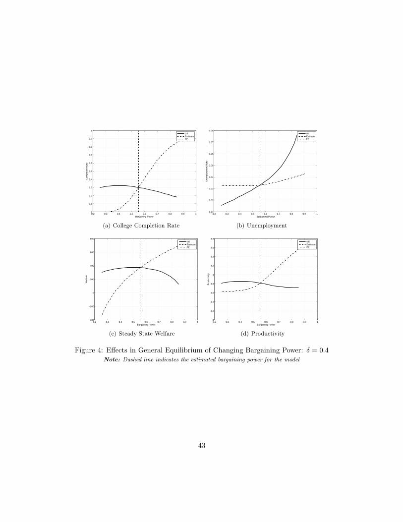
0.2 0.3 0.4 0.5 0.6 0.7 0.8 0.9 10

0.1

0.2

0.3

0.4

0.5

0.6

0.7

0.8

0.9

1

Com

plet

ion

Rat

e

Bargaining Power

GEEstimatePE

(a) College Completion Rate

0.2 0.3 0.4 0.5 0.6 0.7 0.8 0.9 10.01

0.02

0.03

0.04

0.05

0.06

0.07

0.08

Une

mpl

oym

ent R

ate

Bargaining Power

GEEstimatePE

(b) Unemployment

0.2 0.3 0.4 0.5 0.6 0.7 0.8 0.9 1−400

−200

0

200

400

600

800

Wel

fare

Bargaining Power

GEEstimatePE

(c) Steady State Welfare

0.2 0.3 0.4 0.5 0.6 0.7 0.8 0.9 13

3.2

3.4

3.6

3.8

4

4.2

4.4

4.6

4.8

Pro

duct

ivity

Bargaining Power

GEEstimatePE

(d) Productivity

Figure 4: Effects in General Equilibrium of Changing Bargaining Power: δ = 0.4Note: Dashed line indicates the estimated bargaining power for the model

43

0.2 0.3 0.4 0.5 0.6 0.7 0.8 0.9 10

0.1

0.2

0.3

0.4

0.5

0.6

0.7

0.8

0.9

1

Com

plet

ion

Rat

e

Bargaining Power

GEEstimatePE

(a) College Completion Rate

0.2 0.3 0.4 0.5 0.6 0.7 0.8 0.9 10.01

0.02

0.03

0.04

0.05

0.06

0.07

0.08

Une

mpl

oym

ent R

ate

Bargaining Power

GEEstimatePE

(b) Unemployment

0.2 0.3 0.4 0.5 0.6 0.7 0.8 0.9 1−400

−200

0

200

400

600

800

Wel

fare

Bargaining Power

GEEstimatePE

(c) Steady State Welfare

0.2 0.3 0.4 0.5 0.6 0.7 0.8 0.9 13

3.2

3.4

3.6

3.8

4

4.2

4.4

4.6

4.8

Pro

duct

ivity

Bargaining Power

GEEstimatePE

(d) Productivity

Figure 5: Effects in General Equilibrium of Changing Bargaining Power: δ = α = 0.55Note: Dashed line indicates the estimated bargaining power for the model

44

0.2 0.3 0.4 0.5 0.6 0.7 0.8 0.9 10

0.1

0.2

0.3

0.4

0.5

0.6

0.7

0.8

0.9

1

Com

plet

ion

Rat

e

Bargaining Power

GEEstimatePE

(a) College Completion Rate

0.2 0.3 0.4 0.5 0.6 0.7 0.8 0.9 10.01

0.02

0.03

0.04

0.05

0.06

0.07

Une

mpl

oym

ent R

ate

Bargaining Power

GEEstimatePE

(b) Unemployment

0.2 0.3 0.4 0.5 0.6 0.7 0.8 0.9 1−400

−200

0

200

400

600

800

Wel

fare

Bargaining Power

GEEstimatePE

(c) Steady State Welfare

0.2 0.3 0.4 0.5 0.6 0.7 0.8 0.9 13

3.2

3.4

3.6

3.8

4

4.2

4.4

4.6

4.8

Pro

duct

ivity

Bargaining Power

GEEstimatePE

(d) Productivity

Figure 6: Effects in General Equilibrium of Changing Bargaining Power: δ = 0.6Note: Dashed line indicates the estimated bargaining power for the model

45