Universite Paris I - Pantheon Sorbonne

U.F.R. de sciences economiques

Annee 2015 Numero attribue par la bibliotheque

| | | | | | | | | | | | |

THESE

Pour l’obtention du grade de

Docteur de l’Universite de Paris I

Discipline : Sciences Economiques

Presentee et soutenue publiquement par

Chaimaa Yassine

————–

Labor Market Search Frictions in

Developing Countries

Evidence from the MENA region: Egypt and Jordan

————–Directeur de these: Francois Langot

JURY :

Ragui Assaad Professeur a l’Universite de Minnesota

Olivier Charlot Professeur a l’Universite de Cergy-Pontoise (rapporteur)

Nicolas Jacquemet Professeur a l’Universite Paris 1 Pantheon-Sorbonne

Francois Langot Professeur a l’Universite du Maine (directeur de these)

David Margolis Directeur de recherche CNRS

Fabien Postel-Vinay Professeur a l’Universite College London (rapporteur)

L’universite Paris I Pantheon-Sorbonne n’entend donner aucune approbation

ni improbation aux opinions emises dans cette these. Ces opinions doivent etre consid-

erees comme propres a leur auteur.

2

En souvenir de ma grandmere, qui me manque.

A ma mere, qui m’est tellement chere.

A mon cheri, qui me fait vivre les reves les plus merveilleux.

3

Acknowledgements

“Paris has given me what no other city in the world can give to a student (...) The

seed of understanding is in my heart now.” Khalil Gibran to Mary Haskell, March14,

1909. For many, Paris is a tourist destination, a charming city and a symbol for the art

of living. For me, Paris is much more than that. Paris is the city that received me with

wide opened arms, and it did so in every sense: not only education and knowledge,

but more importantly health, friendships and exceptional experiences. I’m grateful to

every moment I’ve spent in the city of lights, which shall always remain my second

homeland.

This thesis is the result of my Ph.D. studies at the University of Paris 1 Pantheon-

Sorbonne during the period September 2011 to December 2015. While my name may

be alone on the front cover of this thesis, I am by no means its sole contributor.

Rather, there are a number of people behind this piece of work who deserve to be

both acknowledged and thanked here: a committed supervisor, generous researchers

and professors, patient friends, an inspiring grandmother, a determined mother and a

fantastically supportive partner.

First and foremost, I would like to offer my sincerest gratitude to my supervisor

Francois Langot for his constant encouragement, support and guidance. I have ben-

efited tremendously from my interactions with him both on the professional and the

personal level, and I owe a great debt to him. His guidance helped me in all the time

of research and writing of this thesis. I could not have imagined having a better ad-

visor and mentor for my Ph.D. study. Francois has taught me, both consciously and

un-consciously, how good quality economic research is done. I appreciate all his con-

tributions of time and ideas to make my Ph.D. experience productive and stimulating.

The joy and enthusiasm he has for his research was contagious and motivational for

4

me, even during tough times in the Ph.D. pursuit.

My passion to labor economics, in general, and to the job search equilibrium theory,

in particular, was primarily inspired by my instructors in the ETE Masters program at

Paris School of Economics, Andre Zylberberg and Fabien Postel-Vinay. I owe a special

thanks to Fabien Postel-Vinay for all the guide and assistance he provided through out

the writing of my Masters’ thesis, the first milestone to this Ph.D. thesis.

I will forever be thankful to Ragui Assaad. Not only that he provided me with a

life-changing experience by getting me involved in the Egypt and Jordan Labor Market

Surveys through their different phases, but he has always been helpful in providing

advice many times during my graduate school journey. Inviting me to spend a semester

at the University of Minnesota definitely provided a valuable plus to my career. Ragui

will always remain as my best role model for a researcher, mentor, co-author and

teacher. I still think fondly of my time as his research assistant at the Economic

Research Forum. A real father, a friend and a colleague, whom I’m very lucky to have

met at the very early years of my career as a labor economist.

I am particularly indebted to David Margolis, whose office had a door that was

wide open all the time for my questions, concerns and doubts during tough times of my

Ph.D. David has been actively interested in my work and has always been available to

advise me. I am very grateful for his patience, motivation, enthusiasm, and immense

knowledge that, taken together, make him a great mentor and a friend.

I am very grateful to the remaining members of my dissertation committee, Olivier

Charlot and Nicolas Jacquemet. Their academic support, input and personal cheering

are greatly appreciated.

Special mention goes to Mona Amer, without whom, this post-graduate journey

would have not been possible. Not only for her tremendous academic support since

my undergraduate studies, but also for helping me out through so many wonderful

opportunities. I owe a lot to Rana Hendy, Chahir Zaki, Jackie Wahba, Caroline Krafft

and Hoda Selim. Apart from being my friends, they were always there providing all

the support, advice and motivation.

Profound gratitude goes to all my professors and colleagues at the MSE in general

and in the microeconomics department in particular. I am also hugely appreciative to

5

Antoine Terracol and Benoit Rappoport, who never hesitated to share their expertise

so willingly. It was always a pleasure to cross Stephane Gautier by the coffee ma-

chine and get the chance to hear one of his amazingly hilarious jokes or comments.

Special mention also goes to Jean-Phillipe Tropeano, Francois Fontaine and Phillipe

Gagnepain.

My gratitude is also extended to Elda Andre and Loic Sorel who have known the

answer to every question I’ve ever asked regarding the aministrative steps of the Gradu-

ate School. The first friendly faces one gets to greet as soon as one begins this doctoral

program. Elda has always been a tremendous help no matter the task or circumstance

and if it weren’t for Loic I wouldn’t have completed all the required paperwork and

delivered it to the correct place at the right timing. Thank you Elda and Loic, you shall

always be remembered as smiling faces, warm and friendly hearts and among the main

people who assisted me in completing my doctoral program. I also greatly appreciate

all the technical support I luckily got from the MSE IT department. Stephane, Rachad

and Rachid were always there, with smiley encouraging faces, whenever the computer

bugs and freaks me out.

This dissertation would have also been impossible without the financial support of

Campus France, the Graduate School of the University of Paris 1 Pantheon-Sorbonne,

the Microeconomics department (UG4) of the Centre d’Economie de la Sorbonne and

the GAINS (Groupe d’Analyse des Itineraires et des Niveaux Salariaux) department

at the University of Maine.

I am indebted to all my friends in Paris who were always so helpful in numerous

ways. Special thanks to Claire Thibout and Rawaa Harati who have always been by my

side since our masters program back in 2009. I’ve enjoyed being surrounded during my

Ph.D. studies by loveable friends like Thomas Fagart, Juliette Rey, Robert Somogyi,

Omar Sene and Batool Syeda. I was also very lucky to have shared the office with the

amazing Marine Hainguerlot, Sandra Daudignon, Pierre Aldama, Antoine Hemon and

Antoine Malezieux. I can never forget the fun lunch breaks and Menagerie weekend

outings with all the MSE Ph.D. students in the different departments, particularly

Elias, Remi, Leontine, Alexandra, Marco, Noemi, Mehdi, Lorenzo, Anastacia and many

others.

6

I show extensive gratitude to all my colleagues at the GAINS laboratory at the

University of Maine in le Mans. Special thanks to my bureau-mates who were always

very good listeners and were a main source of motivation. Big thanks to Jeremy

Tanguy, Eva Mareno-Galbis, Sylvie Blasco, Ahmed Tritah, Pierre-Jean Messe, Salima

Bouayad, Solene Tanguy, Frederic Karame, Xavier Fairise, Jean-Pascal Gayant and

Arthur Poirier. Fun talks and coffee breaks with Jerome Ronchetti, Emmanuel Auvray

and Anthony Terriau shall always be remembered as my recharging stops during my

marathon teaching days in le Mans.

I also owe a lot to all my Egyptian friends present in Paris over the different years

ever since my masters. Gatherings with fine Egyptian dining that I miss made it

impossible for one to feel homesick. Hoping not to forget anyone, I express my gratitude

to Irene Selwaness, May Magdi, Stephanie Youssef, Nelly El Mallakh, Dina Kassab, Rim

Ismail, Ahmed Habib, Mohammed Doma, Omar Monieb, Fady Rizk-Allah, Martine

Ackaad, Nancy Nagui, Heba Mohsen, Tamer Mohsen, Maria Adib, Dina Mandour,

Riham Ezzat and Nesma Magdi.

My thoughts are back home with the irreplaceable best friends, more of sisters,

Maha El Garf, Ghadie El Helaly and Ingy Akoush. Being there in the good and tough

times, they were of great support by all means and over all the levels. They never

hesitated to do everything to draw a smile on my face during peaks of stress, all the

way from sunday morning viber talks and their dogs’ photos that always occupied my

phone memory to getting themselves to Europe just to get on the carroussel infront of

the Eiffel tower together.

I wish my father in law, Magdi Shalash, was there at the moment I am finalizing

this thesis. I am sure he would have been so proud. I would also like to express my

appreciation to a loveable supporting mother in law, Amel Hatem.

I end this aknowledgements’ section with special warm thanks to the three most

important persons in my life: my grandmother, my mother and my fiance.

I owe so much of the person I am today to one great lady who taught me how to

hold a pencil and write down ABC, my grandmother. The loving memory of how tough

she has always been till the very last moment of her life, shall always be my inspiration

throughout my career and personal life. I miss you and I know you’re always there in

7

spirit.

Words can never express how much I’m grateful to one of the greatest mothers

on Earth, Nagwa Nassar. Without her continuous support, love and encouragement I

never would have been able to achieve any of my goals. I owe everything to you mom!

You’ve been the mother, the father, the sister and the friend. Thank you for being my

backbone. It’s time for me to take care of you, make you proud and try to repay a tiny

part of my debt. This one is for you!

The third most special person to my heart is my best friend, my one and only love,

my future husband, Karim Shalash. You have selflessly given more to me than I could

have ever asked for. I love you, and look forward to our lifelong journey. I will end this

by our favorite poem, back in 2007, when we first met.

I shall be telling this with a sigh

Somewhere ages and ages hence:

Two roads diverged in a wood, and I-

I took the one less traveled by,

And that has made all the difference.

Chaimaa Yassine

Paris, December 2015

8

Resume en francais

Les modeles de recherche d’emploi

dans les pays en voie de

developpement

L’elargissement de l’ecart entre les nations est un phenomene inquietant pour tous

les pays du monde et particulierement les pays pauvres en voie de developpement.

En 2010, la distance entre les pays riches et pauvres s’est elargie enormement. Selon

Klugman (2010), le pays le plus riche en 2010 (le Liechtenstein) etait trois fois plus riche

que le pays le plus riche en 1970, pendant que le pays le plus pauvre (le Zimbabwe) est

devenu 25% plus pauvre qu’il etait en 1970 (etant lui-meme le pays le plus pauvre a

l’epoque).

Comme L’ecart entre les richesses des pays ne cesse de se creuser, les politiques

dans les pays en voie de developpement visent a augmenter les opportunites d’emploi

afin d’elever les revenus et les niveaux de vie des populations. Cependant, ces poli-

tiques sont souvent contradictoires. Bien que l’expansion d’emploi devrait soulager la

pauvrete, il n’existe pas de consensus sur les meilleures strategies a adopter dans ces

pays, etant donnee leur caracteristiques assez particulieres. Les reglements et institu-

tions sont necessaires pour proteger les droits des travailleurs et pour ameliorer leurs

conditions de travail. Cependant, ils pourraient en meme temps decourager des en-

treprises a embaucher des travailleurs, ayant alors involontairement une consequence

contradictoire sur les personnes dont les droits et les conditions etaient censes etre pro-

i

teges. D’autre part, les conditions et les politiques d’emploi du secteur public peuvent

contredire ces reglements. Etant donne la stabilite des postes, les ”files d’attente” des

chercheurs d’emplois (chomeurs ou deja employes temporairement) s’allongent pour les

emplois dans ce secteur. Cependant, les realites fiscales et les contraintes budgetaires

des gouvernements rendent ces postes insuffisants pour satisfaire tous les demandeurs

d’emplois. En outre, la non-conformite massive est une norme et les reglements comme

le salaire minimum peuvent encourager l’expansion d’un marche informel non regle-

mente, ou les salaires sont encore moins eleves, l’emploi est beaucoup plus flexible et

non-stable, et les conditions de travail sont encore plus mauvaises.

Les pays arabes du Moyen-Orient et Afrique du Nord (MENA) representent un

groupe special parmi ces pays en voie developpement. Ce sont des pays qui ont recem-

ment connu une vague de soulevements populaires visant a evincer plusieurs presidents

de la region, et faisant suite aux accroissements de la pauvrete, des inegalites et de

l’exclusion (resultats des faibles performances du marche du travail). Malgre la crois-

sance economique observee dans beaucoup de ces pays, cela n’a pas cree suffisamment

d’emplois pour absorber les entrants sur le marche du travail, que cela soit le grand

nombre de jeunes ou bien encore les chocs de main d’oeuvre suite au retour de migrants

comme par exemple apres la guerre en Irak en 2003). De plus, cette croissance a favorise

seulement les emplois de faible qualite avec une faible productivite dans le secteur in-

formel ou de nombreux travailleurs se retrouvent pieges et incapables d’echapper a la

pauvrete.

Ces soulevements ont commence principalement suite a la crise economique mon-

diale en 2008 qui a elle-meme conduit a une erosion des opportunites economiques sur

le marche du travail. Pendant ce temps, des pays comme l’Egypte et la Jordanie ont

ete impliques dans des reformes structurelles de leurs marches du travail au cours des

precedentes 20 dernieres anne qui ont eu surement plusieurs consequences sur leur per-

formance. Par consequent, la comprehension de l’echec de ces institutions et de leurs

reformes a pouvoir garantir des debouches professionnels convenables aux travailleurs

est essentielle pour les decideurs politiques, surtout depuis le printemps arabe ou ils

essayent de repondre a la crise economique et d’offrir des opportunites plus equitables

a leurs populations en colere. Pour etre capable de faire cela, cette these cherche donc

ii

a etudier ces marches du travail specifiques, en particulier l’Egypte et la Jordanie, en

proposant des modeles structurels originaux qui sont confrontes aux faits (estimations

et tests).

La litterature precedente sur les marches du travail de la region MENA en general,

et sur les marches egyptiens et jordaniens en particulier, s’est basee principalement sur

des approches statiques et globales. La recherche scientifique dans la region est faite en

utilisant des enquetes en coupe, pour examiner les stocks et les changements dans ces

stocks. Il existe par contre plusieurs limites a cette methode. Alors que l’on peut etre

en mesure de mesurer la part du marche informel, le chomage et la non-participation,

il devient impossible de repondre a des questions cruciales concernant les transitions

de court et long terme sur ces marches du travail. En effet, le principal probleme en

economie n’est pas de connaitre l’etat qu’occupe un individu dans le marche du tra-

vail. Ce qui importe vraiment est combien de temps cette personne reste dans cet

etat et si jamais il/elle le quitte, quelle sera la destination suivante. L’importance de la

l’analyse des flux sous-jacents les stocks du marche du travail doit etre transmis aux de-

cideurs politiques de la region. D’une part, cela leur permettrait de detecter les points

d’inflexion, d’evaluer les tensions sur le marche du travail et de mesurer les reponses

aux fluctuations du cycle economique, les chocs et les differentes reformes. D’autre

part, pour pouvoir maintenir les taux de chomage le plus bas possible, il est impor-

tant d’assurer un marche du travail assez dynamique ou les creations mais aussi des

destructions existent et ou leurs niveaux sont assez elevees. Cela garantit finalement

une amelioration de la productivite des emplois, car les emplois a haute productivite

sont crees et ceux a faible productivite sont detruits, les travailleurs se reallouant alors

facilement et rapidement vers les emplois efficients. En raison de la nature des don-

nees disponibles et en raison de l’absence d’ensembles de donnees de panel annuelles,

les chercheurs tentent d’etudier la dynamique des marches du travail egyptien en se

concentrant uniquement sur le processus de creation d’emplois, ignorant les destruc-

tions d’emplois et les flux de mobilite entre emplois. Des exemples de cette litterature

pourraient inclure les tentatives pour analyser les durees de chomage (Kherfi, 2015), les

transitions education-travail (Amer, 2014 , 2015 ) et le parcours de transitions de vie

(Assaad and Krafft, 2013). Enfin, les marches du travail egyptiens et jordaniens sont

iii

caracterises par la presence de marches informels flexibles non reglementes. Afin d’etre

en mesure de reduire la difference entre les emplois formels et informels, un marche du

travail formel dynamique et flexible doit etre encourage. Cela reduit l’ecart entre les

emplois formels et informels (qui sont flexibles par definition).

Cette these vise a contribuer a la litterature, tant sur un plan empirique que sur un

plan theorique. Au niveau empirique, ce fut un travail tres fastidieux que de construire

des bases de donnees fiables sur les flux du marche du travail de ces pays, compte tenu de

la non-disponibilite de statistiques officielles, des donnees de panel a frequence courte

ou des faits stylises particuliers, tels que l’emploi informel. Cela a rendu necessaire

d’etudier ces flux a l’aide de toutes les possibles diverses d’approches - des methodes

les plus basiques aux plus sophistiquees. Theoriquement, on propose une extension de

la theorie de la recherche d’emploi classique, pour pouvoir expliquer les phenomenes

paradoxaux dans les pays en voie developpement en raison de leur nature et leurs carac-

teristiques particulieres. Par exemple, il faut tenir compte de leurs secteurs informels,

de la taille non negligeable de l’emploi du secteur public et la corruption. Ce travail

propose aussi d’evaluer les institutions du marche du travail et les reformes structurels

qu’ont connus les marches du travail egyptiens et jordaniens. La these tente donc de

fournir un cadre theorique d’analyse des principales forces conduisant a l’equilibre sur

ces marches, et propose des recommandations politiques pour les decideurs qui ont

besoin de comprendre l’histoire et l’evolution du fonctionnement de leur marche du

travail. L’elaboration de ces outils est d’autant plus importants qu’ils ont besoin de

prendre des mesures correctrices pour accompagner la transition democratique actuelle

de leurs pays.

Tout au long des differentes etapes de chaque chapitre de cette these, on tente de

repondre a trois questions ou problematiques principales. Tout d’abord, est-ce que les

demandeurs d’emploi en Egypte et en Jordanie arrivent a trouver du travail? Des analy-

ses des tendances et de l’evolution dans le temps des creations d’emploi, des separations

et des mobilites entre emplois, sont donc proposes. Ceux-ci comprennent l’utilisation

des donnees microeconomiques disponibles pour extraire des donnees de annuels et

semi-annuels retrospectives. Suivant Shimer (2012), ces donnees microeconomiques

sont ensuite utilisees pour construire les series temporelles macroeconomiques des flux

iv

sur le marche du travail des deux pays (Chapitre 1). Dans le Chapitre 2, ces donnees

de panel retrospectives sont analysees et comparees aux informations sur les memes

individus disponibles en coupe. Cependant, il est demontre dans ce chapitre que ces

donnees de panels sont biaisees par des erreurs de mesure, plus precisement un biais de

memoire. Un des principaux apports de cette these est donc le developpement d’une

methodologie original qui permet de corriger ce biais de memoire a partir des donnees

agregees de flux (Chapitre 3) ainsi que de corriger les transitions et les durees des don-

nees au niveau individuel (Chapitres 5 et 6). Ainsi, en analysant les flux de creations et

de destructions d’emploi, il est monte que les deux marches du travail egyptien et jor-

danien sont tres rigides. Apres ce constat, une deuxieme problematique est alors abor-

dee. Elle a pour objectif d’evaluaer des reformes structurelles introduites sur le marche

du travail et de mesurer leur impact sur les performances et les resultats de ce marche.

Il etait crucial de determiner comment le chomage varie en reponse a l’introduction des

reformes qui visent a flexibiliser le marche et qui rendent les reglements de protection

de l’emploi dans ces marches plus souples. Pour repondre a cette question, on se sert

la reforme visant a liberaliser le marche travail egyptien suite a l’introduction d’une

nouvelle loi en 2003. L’impact a ete analyse empiriquement (dans le Chapitre 3) et

theoriquement (dans les Chapitres 3 et 4). La troisieme et derniere tache de cette these

a ete d’analyser la qualite des emplois auxquels les gens ont acces sur ces marches du

travail. Cela comprenait la caracterisation des flux du marche du travail et l’etude des

changement d’emploi et des avancements des travailleurs dans l’echelle de salaires. Ceci

a ete rendu possible grace a l’estimation de formes reduites appliquant la methode de

correction du biais de memoire (chapitre 5), ainsi qu’a l’estimation d’un modele struc-

turel, permettant alors de reveler les parametres d’appariement du marche du travail

(chapitre 6).

Comme l’analyse des flux est devenue l’outil de base de l’economie du travail mod-

erne, au detriment du paradigme conventionnel de l’offre et de la demande dans un

environnement sans frictions, cette these cherche a expliquer le fonctionnement des

marches du travail egyptiens et jordaniens en utilisant la theorie de la recherche d’emploi

d’equilibre. Il existe deux approches principales pour modeliser la recherche d’emploi

sur le marche du travail. Cette classification depend essentiellement de la nature et de

v

la facon dont les frictions d’appariement sur le marche de travail sont definies, ainsi que

de la maniere dont les salaires d’equilibre sont determines. La premiere approche con-

siste a tenir compte des frictions sur le marche du travail sous la forme d’informations

incompletes sur les postes vacants pour les chomeurs et sur les demandeurs d’emploi

pour les entreprises, ce qui genere un delai entre le debut du processus de recherche et

l’appariement entre un chomeur et un employeur ayant des postes vacants. Diamond

(1982), Mortensen (1982) et Pissarides (1985) ont adopte cette approche. Les salaires

sont determines dans ce cas a travers un processus de negociation de Nash, l’application

de cette solution de Nash pour la determination de salaire d’equilibre etant justifiee

par les travaux de (Binmore, Rubinstein, and Wolinsky, 1986). La deuxieme categorie

de modeles suppose que les frictions ont pour source l’informations incompletes des

travailleurs sur les salaires offerts. Dans ce cas, les travailleurs recoivent des offres,

a prendre ou a laisser (un offre par periode), et ont le choix d’accepter ou de rejeter

l’offre avant de pouvoir en tirer une nouvelle. Les modeles de recherche d’emploi ont

adopte cette approche dans un cadre d’equilibre partiel, cette limite a l’equilibre partiel

resultant des travaux de Diamond (1971). Elle sera depassee suite au developpements

proposes par Albrecht and Axell (1984) et Burdett and Mortensen (1998): les salaires

sont alors determines par des monopsones (les entreprises), les employes ayant quant

a eux le “pouvoir” d’etre mobiles ce qui permet de sortir de la critique de Diamond

(1971) sur la degeneressance de l’equilibre dans un modele de recherche d’emploi.

L’evaluation des dynamiques des entrees et des sorties du chomage est possible

en utilisant la premiere approche ou les taux de transitions peuvent etre obtenus en

fonction de la tension du marche du travail, l’intensite de la recherche des travailleurs,

etc...(Pissarides, 1990). Les Chapitres 3 et 4 choisissent donc d’adopter cette approche

en essayant de comprendre la nature de la dynamique du marche du travail egyptien.

Ils visent a etudier si les travailleurs arrivent a trouver un emploi ou non, et comment

les emplois sont detruits. Cette methode ne permet pas toutefois de decrire la qualite

des emplois et les avancements des travailleurs dans l’echelle des salaires. C’est une

methode qui est donc moins informative sur les distributions de salaires et aucune

fonction de salaires offerts endogene peut etre obtenue. Les applications empiriques de

cette approche sont par consequent limitees aux problematiques macroeconomiques. En

vi

revanche, la seconde approche adopte un modele ou les distributions de offres salariales

sont endogene et permet de deminer la distribution unique des salaires de l’economie.

La distribution des offres de saliare est un element crucial qui facilite l’estimation

et l’application empirique du modele. Le Chapitre 6 choisit de se concentrer sur la

deuxieme classe de modeles.

Le manuscrit de these est divise comme suit.

Chapitre 1

Le Chapitre 1 est introductif, et a pour principal objectif de decrire les principales

eolutions obsrevees, ainsi que d’etablir un certain nombre de faits et descriptifs ma-

jeurs, sur l’histoire recente de ces flux du marche du travail egyptiens et jordaniens. Le

chapitre fournit les grandes lignes directrices sur la methologie suivie pour construire

les bases de donnees. En particulier, la facon dont les donnees de panel retrospectives

semestrielles et annuelles sont extraites pour l’Egypte et la Jordanie en utilisant les

enquetes disponibles du marche du travail (ELMPS et JLMPS). Ces donnees de panel

retrospectives seront utilises tout au long de la these. Le chapitre fournit egalement un

resume des cadres institutionnels des deux pays. Il examine les statistiques descriptives

des flux du marche. Ils soulignent les similarites et les differences entre ces deux pays.

Les conclusions de ce chapitre sur la dynamique des marches du travail egyptiens et jor-

daniens ne sont pas rassurantes. Celles-ci montrent que les taux de creations d’emploi

et de separations sont extremement faibles dans les deux economies. Meme, pour les

transitions entre emplois, elles ne s’observent en gande partie que dans les secteurs

informels ou les offreurs de travail peuvent trouver un moins bon emploi que precede-

ment plutot que de devenir plus productif et d’ameliorer leur position dans l’echelle

des salaires. Cependant, le marche du travail jordanien semble etre relativement plus

flexible que le marche du travail egyptien. Par contre, avec des petites differences entre

le taux de creations dans les secteurs formels et informels jordaniens, les chiffres et les

tendances observees suggerent que le marche du travail jordanien est plus segmente que

l’Egyptien.

L’objectif du Chapitre 1 est de definir un certain nombre de faits stylises sur les flux

vii

du marche du travail egyptien et jordanien durant la derniere decennie en utilisant les

donnees ”Egypt Labor Market Panet Survey” (ELMPS) et ”Jordan Labor Market Panel

Survey”(JLMPS). Bien qu’il soit descriptif, la contribution principale de ce chapitre est

de fournir un resume d’un large eventail d’informations sur la dynamique des marches

du travail egyptien et jordanien a partir de plusieurs angles differents. Le document

fournit un apercu des differentes institutions du marche du travail en Egypte et en

Jordanie. Ce sont des marches generalement caracterises par de faibles niveaux de

l’emploi, un taux de chomage eleve parmi les jeunes, des secteurs publics de grande

taille et des marches informel, non-reglementes par le gouvernement, consequents. Il

fournit egalement une description de la structure des questionnaires des donnees qui

vont etre utilises dans cette these. Il detaille la methodologie adoptees pour extraire les

donnees de panel retrospectives. Cette methode d’extraction de donnees de panel est

cruciale pour les pays en voie de developpement tels que l’Egypte et la Jordanie, ou les

contraintes budgetaires ne permettent pas la collecte de donnees de panel regulierement,

ce qui est necessaire pour l’analyse de la dynamique du marche du travail.

Les faits stylises deduits sur la dynamique du marche du travail sont les premiers de

ce genre et peuvent se reveler utiles pour les chercheurs et les decideurs politiques qui

travaillent sur les divers aspects des marches du travail egyptiens et jordaniens. Comme

deja mentionne, la connaissance de ces faits est cruciale pour pouvoir suivre les cycles

economiques, detecter des points d’inflexion et d’evaluer la tension du marche du tra-

vail (comment la demande de main-d’oeuvre et l’offre “s’equilibrent” dans l’economie).

Il est important d’assurer un marche du travail sain et dynamique ou les emplois pro-

ductifs sont crees et les emplois moins productifs sont detruits, les emplois existants

devenant alors plus productifs en moyenne. Cela ne semble pas etre le cas du tout sur

les marches egyptien et jordanien travail ou la plupart du chiffre d’affaires se realise via

les emplois du secteur informel, les taux de transitions d’emploi a emploi etant quant

a eux extremement faibles. Si ces transitions se produisent, c’est parce que les gens se

deplacent a l’interieur ou vers le secteur informel. Il faut noter cependant que le marche

du travail jordanien, compte tenu de l’histoire et l’evolution de son cadre institutionnel,

est plus souple et plus flexible que le marche du travail egyptien. Pourtant, il existe

des faits qui suggerent que le marche du travail jordanien est beaucoup plus segmente

viii

que l’Egyptien; le secteur informel servant surtout comme un intermediaire en Egypte,

en Jordanie, il semble etre un segment du marche qui fonctionne sur ses propres tra-

vailleurs. L’aspect informel de deux marches necessite surement des recherches plus

avancees.

En Egypte, les secteurs public et prive formel souffrent d’un environnement extreme-

ment rigide ou les travailleurs, une fois qu’ils accedent a des emplois dans ces secteurs,

ne quittent jamais ni ne passent a d’autres emplois. En general, les taux de separations

en Egypte sont extremement faibles. Les tendances des flux dans ce chapitre mon-

trent cependant qu’il y a eu de meilleures reponses au ralentissement economique du

secteur prive formel qu’auparavant, surtout apres la revolution du Janvier 2011. Dans

l’ensemble, la rigidite des marches du travail egyptiens et jordaniens fait baisser dans

une large mesure les niveaux de productivite et la croissance au sein de l’economie.

Les principales conclusions de ce chapitre confirment le fait que le chomage en

Egypte tend a etre domine par le chomage structurel plutot que le cyclique. Les ten-

dances obtenues a partir des donnees brutes pourraient suggerer un role croissant du

chomage conjoncturel sur le marche du travail egyptien apres 2009, suite a la crise finan-

ciere ainsi que la revolution Janvier 2011. En Jordanie, les composantes de chomage, les

creations et les separations ont connu un changement remarquable dans les tendances

apres 2003, soit apres le retour des Jordaniens apres la guerre en Irak et egalement

apres le ralentissement des taux de croissance (la baisse du PIB) en 2007. Les marches

du travail egyptien et jordanien sont deux pays arabes de la region MENA qui souf-

frent d’un niveau tres faible de creations, de separations et de mobilite relativement aux

stocks de l’emploi et du chomage. Le chapitre note une tendance a la baisse dans les

taux d’embauche egyptiens, refletant la tendance a la baisse dans le taux de croissance

de la population en age de travailler, montrant que l’explosion de la jeunesse a ete

absorbe avec succes dans le marche du travail egyptien cours de la derniere decennie. Il

montre egalement une tendance constante de creations de l’emploi en Jordanie suivant

le taux de croissance de la population stagnante. Cependant, les tendances montrent

qu’il est devenu plus difficile pour un individu non-employe a trouver un boulot. La

probabilite que les travailleurs quittent leur emploi ou soient licencies reste tres faible

meme apres une augmentation apparente dans les annees les plus recentes des donnees

ix

de panel retrospectives, c’est a dire dans les annees juste avant l’annee de l’enquete. Il

faut etre prudent lors de l’analyse de ces resultats compte tenu des biais potentiels et

des erreurs de mesure dans les series de donnees utilisees qui pourraient entraıner des

variations artificielles du niveau ou des tendances. En effet, les resultats suggerent que

les taux de separation atteignent le niveau le plus eleve en 2011 en Egypte et 2010 en

Jordanie, mais cela ne represente que 2 % de l’emploi total en Egypte et 4 % en Jor-

danie. L’analyse montre que la part de la perte d’emploi involontaire a augmente sur

la periode 2009-2011 en Egypte. Cela soutient que ces tendances refletent la reponse

du marche du travail egyptien a la crise financiere et la revolution de Janvier 2011

plutot que d’un marche du travail qui est devenu plus dynamique. Cependant, on ne

peut pas confirmer cette conclusion etant donne les biais de memoire potentiels et les

prejuges de la conception de la questionnaire. Les chapitres suivants examinent ces

erreurs et offrent des solutions et des corrections possibles pouvoir utiliser les donnees

dans l’analyse de la dynamique du marche du travail en question.

L’analyse montre egalement qu’il y a une tendance croissante dans les taux de

transitions entre emplois en Egypte, en particulier parmi les travailleurs du secteur

informel. En general, le secteur formel reste rigide malgre que les reponses au ralen-

tissement economique du secteur prive formel, ainsi que du secteur public, ont ete

observees. Les conclusions du chapitre suggerent que les marches du travail egyptiens

et jordaniens devraient etre une source d’inquietude. Le taux de chomage dans l’avenir,

en particulier en Egypte, devrait etre sensiblement plus eleve en raison des separations

croissantes et des embauches decroissantes, ainsi que les pressions demographiques plus

eleves resultant de l’echo de l’explosion de la jeunesse.

Chapitre 2

La litterature precedente comme Artola and Bell (2001), Bound, Brown, and Math-

iowetz (2001), et Magnac and Visser (1999a) montrent que les donnees retrospectives

basees sur des declarations individuelles souffrent de problemes tels que les difficultes

de se rappeler des dates ou meme de certains evenements. Les donnees de panel sont

des donnees qui sont recueillies simultanement en differents points du temps pour un

x

meme individu. Elles evitent ce probleme parce qu’elles sont collectees a des points

discrets dans le temps. Cependant, elles ne fournissent que des informations sur ces

points dans le temps et non pas sur le cours des evenements entre ces points (Blossfeld,

Golsch, and Rohwer, 2012). Ces donnees sont aussi susceptibles de souffrir d’attrition

de l’echantillon et des erreurs de classification (Artola and Bell, 2001). Dans le chapitre

2, en raison de ces problemes potentiels avec les donnees retrospectives et les donnees

de panel, il devient interessant de comparer les resultats sur les indicateurs de base lies

a la dynamique du marche du travail a partir de donnees de panel retrospectives et

contemporains sur le meme echantillon de personnes, afin de determiner les conditions

dans lesquelles ils fournissent des resultats similaires ou sensiblement differentes. a ce

jour, aucune etude n’a fait une telle comparaison dans la region MENA. Ce chapitre

profite donc d’une occasion unique de pouvoir realiser une telle comparaison, ou a la

fois des donnees de panel et des donnees retrospectives sont disponibles pour les memes

individus en utilisant les vagues de l’enquete d’emploi du marche du travail egyptien

ELMPS 1998, 2006 et 2012. Non seulement les periodes des donnees retrospectives

de chaque vague se chevauchent avec les dates des vagues precedentes, qui permet des

comparaisons de donnees retrospectives et de panel au meme point dans le temps, mais

les periodes retrospectives de differentes vagues de l’enquete se chevauchent les uns avec

les autres ainsi, permettant des comparaisons des evenements passes dans une vague

avec les memes evenements passes captures dans une autre vague. Dans les pays, ou

les budgets de collecte de donnees representent un gros probleme, ce chapitre cherche

donc a demontrer s’il est possible de recueillir des informations sur la dynamique du

marche du travail a l’aide de donnees retrospectives ou est l’erreur de rappel si grand

telles que les donnees de panel soient la seule option viable. Les resultats montrent

qu’il est possible bien que la prudence est necessaire sur le type d’informations conclu

a partir de l’analyse et le niveau de detail utilise dans l’analyse (pour la differenciation

par exemple entre les categories tres detaillees, telles que les travailleurs independants

et les employeurs ou les travailleurs reguliers et irreguliers, cela peut etre trompeur).

Les periodes d’emploi passees obtenues a partir de donnees retrospectives semblent etre

assez fiables tandis que aucunes distinctions fines entre les differents etats du secteur

de l’emploi ne sont faites. Les periodes du non-emploi (chomage et hors de la popula-

xi

tion active) surtout entre les periodes d’emploi, sont toutefois difficile de se rappeler.

Les questions retrospectives suscitant des montants monetaires se sont averes peu fi-

ables. Les repondants ont tendance a gonfler, en actualisant le montant a leur valeur

equivalente au moment de l’enquete.

Ce chapitre fournit egalement des lignes directrices et des lecons sur la facon dont

il faut utiliser les donnees retrospectives existantes de l’enquete ELMPS ou d’autres

enquetes similaires. Tout d’abord, en comparant les donnees retrospectives a par-

tir de ELMPS 2012 aux donnees des vagues precedentes, on a determine qu’il est

preferable de poser des questions sur la trajectoire du marche du travail de l’individu

dans l’ordre chronologique plutot que l’ordre inverse. Il suscite une meilleure informa-

tion sur l’insertion sur le marche du travail et en particulier a propos de toute periode

de chomage initiale avant le premier emploi. Deuxiemement, les resultats montrent

que de nombreux repondants (et meme parfois des enqueteurs) ont mal-interpretees les

modules retrospectives pour signifier juste leur statuts d’emploi, ce qui a contribue a la

sous-declaration retrospective des periodes de chomage et non-emploi. Il est probable-

ment une bonne idee de demander explicitement de savoir s’ il y avait un non-emploi

initial ou periode de chomage avant le premier emploi et a demander explicitement si

la fin de chaque travail a ete suivie par une periode de non-emploi qui a depasse une

duree d’un a six mois. Troisiemement, il est necessaire de demander aux individus qui

ont jamais travaille et sont actuellement inactifs pour savoir s’ils ont jamais cherche de

l’emploi et la duree de la periode dans laquelle ils etaient a la recherche d’emploi, au

moins pour la premiere fois. Quatriemement, bien que l’ajout d’un calendrier des evene-

ments de la vie, qui suscite des informations sur les dates de debut et de fin de tous les

etats du marche du travail contribue a combler certains evenements manquants, il peut

toujours etre utile pour obtenir des informations dans le module retrospectif du marche

du travail en ajoutant un cinquieme et eventuellement sixieme etat du marche du travail

pour capturer les transitions des individus qui bougent beaucoup sur le marche.

Compte tenu des contraintes budgetaires et de disponibilite, les donnees de panel

retrospectives sont actuellement les seuls donnees de panel disponibles dans la region

MENA qui permettent aux chercheurs d’etudier la dynamique du marche du travail,

particulierement les transitions ou les flux a court terme. Apres avoir discute les er-

xii

reurs de mesures et les biais dans les donnees retrospectives, il est toutefois important

de noter qu’il est possible d’utiliser certains remedes qui attenuent ces erreurs de mesure

et, eventuellement, produisent des resultats non-biaises (ou peut-etre moins biaises).

Une solution possible serait de faire un appariement entre les moments biaises obtenus

a partir de donnees retrospectives avec des moments precis et fiables obtenues a par-

tir de donnees transversales contemporaines auxiliaires. Bien sA»r, cela pourrait etre

obtenu a partir des donnees de la meme enquete ou d’une source de donnees externe,

tant que la comparabilite entre les differentes bases de donnees est verifiee et main-

tenue. Dans ce cas, on suppose que les informations obtenues a partir des donnees

transversales (en coupe) est les plus precises. Les hypotheses sur la forme (fonction-

nelle) du taux d’oubli ou de la perte de l’information dans les donnees retrospectives

seraient egalement necessaires. Le Chapitre 3 corrige les taux de transition (au niveau

macro) du marche du travail ELMPS entre emploi, chomage et inactivite, obtenus a

partir des donnees de panel retrospectives, en utilisant cette methode. Ils supposent

que l’annee la plus recente du panel retrospectif est la plus exacte et que les repon-

dants rapportent les evenements les plus lointains avec moins de precision. L’erreur de

mesure a une forme fonctionnelle qui augmente de facon exponentielle que l’on remonte

dans le temps. Cette methodologie peut permettre la reconstruction des matrices de

transitions (taux d’embauche et de separation) corrigees et donc les series temporelles

de ces flux qui peuvent etre utilisees dans l’analyse des tendances macro-economiques

du marche du travail. Cela peut meme etre etendu pour faire usage de l’information

au niveau micro disponible sur les transitions sur le marche du travail. En utilisant les

erreurs de mesure agregees estimees pour les differents types de transitions, on pourrait

distribuer ces erreurs dans la forme de poids aux individus de l’enquete (Chapitre 5).

Encore une fois, des hypotheses doivent etre faites sur la maniere dont on attribue les

poids aux individus. Le Chapitre 5 traite donc deux facons de le faire: (1) une methode

naive: ou tous les individus sont supposes etre corrigees avec des poids similaires, c’est

a-dire proportionnels et (2) une methode differenciee: ou les poids sont predits en se

basant sur la probabilite d’un individu pour faire un certain type de transition. Tout

ce qui precede suppose que l’information dans les donnees de panel retrospectives est

correcte, juste un peu plus rapporte ou sous-declares par rapport aux vrais en coupes

xiii

(les moments non-baise). Une autre solution possible, avec une hypothese differente,

serait d’estimer le taux d’alignement, peut-etre le taux de dire la verite, et, eventuelle-

ment, la creation d’un poids tel que les individus qui declarent la verite ont un poids

plus eleve. Cela necessite cependant la disponibilite a la fois au niveau micro des infor-

mations transversales en coupe et retrospectives pour les memes individus. Dans notre

cas, il pourrait etre applique en Egypte en utilisant les differentes vagues de l’enquete

ELMPS mais pas aux autres bases de donnees, par exemple l’Enquete sur le marche du

travail de la Jordanie (JLMPS) juste une seule vague est disponible. Les inconvenients

de la representativite de l’echantillon peuvent etre discutes apres l’ajout de ces poids.

Une solution possible pour la sous-declaration des etats du marche du travail tels que

le chomage et le non-emploi serait de mettre en accent la bonne interpretation des etats

retrospectifs dans la formation des enqueteurs. En outre, il est suggere d’ajouter des

questions sur les dates de fin de chaque etat tout au long du module retrospectif plutot

que de compter sur la date de debut de l’etat suivant. Meme si les gens interpretent

l’etat retrospectif comme un statut d’emploi, cette information supplementaire pourrait

aider a capturer l’etat de non-emploi interimaire, qui commence a la date de la fin d’un

certain emploi et se termine a la date de debut de l’emploi suivant.

Pour conclure, les donnees de panel avec des modules retrospectifs courts pour

combler les lacunes entre les vagues du panel sont les meilleures donnees que l’on peut

esperer, faute de donnees administratives continues, pour etudier la dynamique du

marche du travail. Cependant, en l’absence de telles donnees de panel, des informations

utiles peuvent etre obtenues a partir des questions retrospectives, tant que certaines

des lecons tirees dans ce chapitre sont gardees en tete.

Chapitre 3

Apres avoir examine les donnees et leurs enjeux dans la premiere partie, la deux-

ieme partie de cette these est consacree a l’evaluation de l’impact de l’introduction de

reformes structurelles qui visent a flexibiliser le marche du travail et donc rendent les

reglements de protection de l’emploi plus souples. Le Chapitre 3 propose d’evaluer une

reforme egyptienne qui a ete introduite en 2003, ayant comme but d’ameliorer et de

xiv

flexibiliser les processus d’embauche et de licenciement. En general, une seule etude

precedente par Wahba (2009) a etudie l’impact a court terme (apres deux ans) de la

loi, mais sur le processus de formalisation en Egypte. Dans ce chapitre, les enquetes du

marche du travail en Egypte (ELMPS 2006 et ELMPS 2012) sont utilisees pour mesurer

l’impact de cette reforme sur la dynamique des taux de separation et de recherche

d’emploi, et pour quantifier leurs contributions a la variabilite du taux chomage global.

L’analyse utilise des donnees de panel retrospectives extraites et creees a partir des

modules retrospectifs dans les enquetes de 2006 et 2012. En superposant les deux pan-

els de deux enquetes, le chapitre estime les probabilites, annuelles et semi-annuelles,

de transitions des travailleurs entre l’emploi, le chomage et l’inactivite. Un modele

originale est propose pour corriger le biais de memoire et de la conception observes

dans les transitions sur le marche du travail obtenus a partir de donnees retrospec-

tives. En utilisant les donnees ”corrigee”, il est alors montre que la reforme augmente

significativement le taux de separations en Egypte, mais n’au aucun effet significatif

sur les taux d’embauche. L’effet combine net est donc une augmentation des niveaux

de taux de chomage egyptien: ou les separations augmentent alors que les embauches

restent inchanges. Cet echec partiel de la liberalisation du marche du travail egyp-

tien est ensuite explique theoriquement par un effet d’eviction suite a l’augmentation

des coA»ts de mise en place, interprete comme une capture par l’agent corrompu du

nouveau surplus, dans le cadre du modele conventionnel de Mortensen and Pissarides

(1994).

L’histoire des institutions dans la plupart des pays en voie de developpement a

conduit leurs marches du travail a etre tres rigides, ou les contrats du secteur prive

ont approche les regles d’embauche du secteur public. Les grandes organisations in-

ternationales ont donc encourage les reformes structurelles, afin d’introduire plus de

flexibilite dans ces marches du travail. L’importance d’assurer un marche sain et dy-

namique du travail reside dans la creation d’emplois plus productifs et en detruisant les

moins productives (voir Veganzones-Varoudakis and Pissarides (2007)). La flexibilite

du marche du travail diminue ainsi la difference entre l’emploi formel et l’emploi in-

formel, qui est tres flexible par definition. En attirant plus de travailleurs a des emplois

formels, les creations des postes dans le secteur formel permet une augmentation des

xv

recettes fiscales des gouvernements et donc reduit leurs deficits budgetaires.

L’importance d’un marche du travail plus flexible a ete reconnue par le gouverne-

ment egyptien en 2003, ou ils ont introduit une nouvelle loi du travail (No. 12). La

nouvelle loi du travail egyptienne a ete implementee en 2004 ayant comme but la

flexibilisation de l’embauche et de licenciement en Egypte. La loi prevoit des lignes di-

rectrices completes pour le recrutement, l’embauche, la remuneration et le licenciement

des employes. Il aborde directement le droit de l’employeur de resilier le contrat d’un

employe.

La theorie economique predit, par contre, des effets ambigus de l’augmentation de

la flexibilite sur la performance des marches du travail. En effet, lorsque le changement

de politique est parfaitement prevu, le modele classique de Mortensen and Pissarides

(1994) montre que si on facilite les licenciements, ceci entraıne une hausse des taux

d’embauche, mais il a aussi un effet positif direct sur les transitions de l’emploi vers

le chomage. Comme le taux d’emploi est une fonction croissante du taux d’embauche,

mais une fonction decroissante de separations, l’evaluation d’une politique qui augmente

la flexibilite du marche du travail necessite l’analyse des differentes elasticites de ces

deux taux de transitions a la reforme en question. Meme si le changement de politique

est inattendu, etant donne que les embauches et les separations sont des variables de

saut “jump (c’est a dire qui reagissent tout de suite), le meme raisonnement est valable.

Meme si les effets sur le chomage sont ambigus, la liberalisation du marche du travail

favorise les creations d’emploi et donc une productivite plus elevee.

Il devient donc essentiel d’evaluer l’ajustement des taux de separation et d’embauche

en Egypte (les deux composantes du taux de chomage egyptien) a une telle reforme de

liberalisation du marche du travail, introduite par la nouvelle loi du travail de 2003. Le

chapitre est en mesure de repondre aux questions de recherche suivantes:

1. Etudier l’evolution des tendances des flux des travailleurs au cours de la periode

1998-2012, et de lier les changements dans les taux de creations et les taux de

separation a la nouvelle legislation du travail egyptienne implementee en 2004.

2. Construire un modele qui nous permet de simuler les politiques du marche du

travail et d’examiner leurs implications sur la dynamique du marche du travail

xvi

egyptien 1

D’un point de vue methodologique, la construction des transitions observees sur le

marche a partir de donnees microeconomiques, developpe par Shimer (2005 , 2012),

semble etre le plus convenable pour evaluer ce type des reformes du marche du travail.

C’est une methodologie qui permet d’exploiter les enquetes du marche du travail riches,

de demeler les changements dans toutes les transitions et d’en deduire en utilisant un

simple equilibre des flux, l’impact sur les agregats, tels que le taux de chomage. Dans

ce chapitre alor, on essaye d’utiliser cette methode de construction, afin de creer les

series macro des flux du marche du travail via des enquetes microeconomiques suivant

le tracail de Shimer. D’un point de vue econometrique, la reforme sera analysee comme

une rupture structurelle dans les series des taux de creations d’emploi et de separatio.

L’effet global sur le chomage sera deduit de la composition des effets differencies des

taux de transition. L’originalite du travail reside dans la construction des series tem-

porelles des flux et donc la dynamique du marche du travail egyptien. Comme dans

la plupart des pays dans le projet du developpement, les enquetes micro (panel) qui

retracent l’histoire de chaque individu chaque mois ne sont pas disponibles. Seule une

enquete du marche du travail ou les individus declarent leurs comptes retrospectifs et

actuels de leurs etats du marche du travail est repetee presque tous les 6 ans. Meme

avec des methodes de la collecte de donnees de haute qualite et des questions de vali-

dation precises, l’information retrospective obtenue de telles enquetes est soumise a un

biais de memoire. De Nicola and Gine (2014) ont montre que la grandeur de l’erreur

de rappel augmente avec le temps, en partie parce que les repondants ont recours a

l’inference plutot que la memoire. Leurs conclusions sont fondees sur une comparaison

entre les donnees administrativs et les donnees d’enquetes retrospectives dans un pays

en voie developpement, plus precisement un echantillon de menages independants en-

gages dans la peche cotiere en Inde. En utilisant les donnees d’un pays developpe (les

Etats-Unis), Poterba and Summers (1986) trouvent a travers une etude sur les enquetes

d’emploi que la correction des erreurs de mesure peut modifier la duree de chomage

estime par un facteur de deux. Ainsi, la contribution methodologique de ce chapitre

1Ceci peut etre fait sans aucun probleme concernant la critique de Lucas (1976) parce que lestaux d’embauches et de separations sont des variables de saut, et etant donne que le changement depolitique est inattendu.

xvii

est de proposer une methode originale pour corriger cette ce biais de memoire, en util-

isant la structure markovienne des transitions sur le marche du travail. On estime de

maniere structurelle, en utilisant la methode des moments simules (SMM), une fonc-

tion representant le taux d’oubli conditionnelle sur l’etat de l’individu sur le marche du

travail. Notre modele est proche de celui developpe par Magnac and Visser (1999b).

Compte tenu de l’importance de prendre en consideration l’entree et la sortie de la pop-

ulation active, et pour pouvoir refleter le vrai portrait du marche du travail egyptien,

on ajoute a l’analyse un modele a trois etats du marche du travail (emploi, chomage et

inactivite). On verifie alors si les resultats sur le taux de chomage, reconstruits a partir

des series de flux du marche du travail corrigees, sont compatibles et robustes. L’etude

montre que les estimations des flux corriges donnent alors des resultats similaires, ce

qui suggere que la methode de correction proposee produit des series robustes. Par

consequent, on peut conclure que la methode peut etre appliquee a plusieurs enquetes

disponibles uniquement entre deux dates relativement espaces, ce qui est souvent le cas

dans les pays en developpement.

Dans son article de 2012, Shimer montre que la reconstruction des series macro

des flux des travailleurs via des enquetes microeconomiques montre que les creations

representent la source principale dans les fluctuations des taux de chomage des etats-

Unis. Ses resultats contrastent donc avec ceux obtenus par Blanchard and Diamond

(1990) et Davis et Haltiwanger (1990, 1992): ces auteurs ont montre que, sur la base

des statistiques de creations d’emplois et de destructions (flux de travail), le majorite

des fluctuations dans le taux de chomage americain sont les resultats des variations du

taux de de separations. Dans ce chapitre, en depit de l’utilisation d’une methodologie

similaire a celle proposee par Shimer (2012), on montre que la nouvelle loi du travail

de 2003 a eu des effets positifs significatifs sur les taux de separation, mais aucun

effet sur les taux d’embauche. L’augmentation du taux de separations donc l’emporte

sur la non-variation du taux d’embauches conduisant a une augmentation du taux de

chomage apres la reforme. Ces resultats restent valables meme apres l’ajout de l’etat

d’inactivite a l’analyse. L’etude des contrefactuels, montre le role dominant des taux

de separation dans les variations du chomage egyptien. Cependant, il est important

de noter que les taux de separations et de creations d’emploi demeurent a des niveaux

xviii

extremement faibles, confirmant la nature tres rigide du marche du travail egyptien.

Ces resultats empiriques peuvent etre considerees comme incompatibles avec le mod-

ele classique du Mortensen and Pissarides (1994), ou une augmentation de la flexibilite

du marche du travail (modelisee comme une baisse des coA»ts de licenciement) serait

certainement suivi par une augmentation des separations et des creations d’emploi.

En effet, une telle politique qui reduit les distorsions fiscales dans le marche devraient

permettre l’augmentation du surplus du A« job match A» (meme si la duree du travail

sera reduite), et par consequent le taux d’embauches. a ce stade, il devient donc difficile

d’expliquer le non-changement du taux d’embauches, en utilisant le modele convention-

nel du Mortensen and Pissarides (1994). Il est vrai qu’on peut expliquer ce phenomene

par le delai entre la reaction des employeurs a la reforme en virant les travailleurs non-

productifs tout apres la mise en oeuvre de la politique, mais en n’embauchant plus de

travailleurs que quand ils se sentent suffisamment confiants sur le marche. Cependant,

parmi les explications possibles derriere un tel phenomene paradoxal pourrait etre le

fait que l’Egypte est un pays en developpement ou la corruption est l’un des principaux

obstacles aux creations d’emplois. Le chapitre essaie donc de montrer theoriquement

comment le modele du Mortensen and Pissarides (1994) peut etre adapte pour ren-

dre compte de ce phenomene et donc expliquer les donnees egyptiennes. Une autre

facon d’expliquer ce puzzle est de proposer une extension du modele Mortensen and

Pissarides (1994) pour tenir compte des secteurs informel et public, qui representent

de grandes parts de l’emploi en Egypte. Meme si la politique est dirigee vers le secteur

prive formel, il affecte certainement l’interaction et la circulation des travailleurs en-

tre les differents secteurs d’emploi. Le modele classique du Mortensen and Pissarides

(1994) n’arrive pas a expliquer ces transitions intersectorielles. Le Chapitre 4 pro-

pose donc un modele de recherche d’emploi a la Mortensen and Pissarides (1994) pour

modeliser les differentes transitions entre les secteurs formel, informel et public pour

pouvoir expliquer les raisons possibles pour que juste les separations augmentent suite

a la liberalisation du marche su travail.

xix

Chapitre 4

Le Chapitre 4 essaye donc d’aller plus loi dans l’analyse et propose d’expliquer

dans quelle mesure le modele de Mortensen and Pissarides (1994) est applicable aux

pays en voie de developpement, tels que l’Egypte, ou les grandes parts des travailleurs

se trouvent dans les secteurs informel et public. Limiter l’analyse, comme dans la

litterature traditionnelle precedente, a seulement un marche du travail prive et non

segmente pourrait etre insuffisant pour les differentes transitions entre secteurs sous-

jacentes et donc ne reflete pas la nature particuliere des marches du travail de la region

MENA. Il existe des essais recentes d’inclure dans le modele de recherche d’emploi un

secteur informel (comme Albrecht, Navarro, and Vroman (2009), Meghir, Narita, and

Robin (2012), Bosch and Esteban-Pretel (2012), Charlot, Malherbet, and Ulus (2013,

2014) et Charlot, Malherbet, and Terra (2015)) ou un secteur public et un secteur prive

non segmente (Burdett (2012), Bradley, Postel-Vinay, and Turon (2013)). Le Chapitre 4

de cette these vise par contre a ajouter a la fois le secteur informel ainsi le secteur public.

Les choix d’emploi/non-emploi d’un travailleur sont donc bases sur les comparaisons

entre ses valeurs d’emplois attendues dans son emploi actuel ou ses emplois potentiels

eventuels, c’est a-dire dans l’un des trois secteurs d’emploi. Le modele construit prend

egalement en consideration les realites fiscales, donc la contrainte budgetaire du secteur

public. Il est vrai que le secteur public peut augmenter ses salaires, mais compte

tenu de sa contrainte budgetaire, il est susceptible de diminuer ses embauches des

employes. Ce qui pourrait se faire, comme en Egypte par exemple, en rationnant

les postes vacants dans le secteur public. Ce chapitre permet donc d’offrir une autre

explication au paradoxe empirique observe dans le chapitre 3 suite a l’introduction

d’une novelle loi en Egypte qui vise a liberaliser le marche du travail. Meme si la

politique est dirigee vers le secteur prive formel, il influence certainement l’interaction

et la circulation des travailleurs entre les differents secteurs d’emploi. Une analyse

qualitative est proposee, ou le modele est calibre et des simulations pour l’impact

des reformes structurelles, en particulier de la loi de 2004 Egypte, sont fournis. Les

resultats sont memes confirme via les donnees disponibles sur les flux en Egypte entre les

secteurs de l’emploi et le chomage, avant et apres la reforme de 2004. Les principaux

xx

resultats suggerent que l’introduction regles de protection de l’emploi plus flexibles,

modelisee par une reduction des couts de licenciements, favorise la creation d’emplois

et la destruction d’emplois dans le secteur prive formel qui est le but principal de la

politique. Il augmente les separations d’emploi dans le secteur informel et diminue les

embauches informelles. En effet, il est demontre que la liberalisation du marche du

travail egyptien joue contre l’emploi informel en augmentant la rentabilite des emplois

formels. Mais, si les salaires offerts par le secteur public augmentent en meme temps que

la loi, comme ce qui est arrive en Egypte (Said, 2015), cela creerait un effet d’eviction,

ou le nouveau surplus cree par la reforme est que compensee par les nouveaux coA»ts

de la mobilite des travailleurs induits par l’augmentation de l’attractivite du secteur

public. Ce resultat est robuste, meme si la baisse des couts de licenciement diminue la

proportion de la recherche des travailleurs deja en emploi dans les secteurs formels et

informels, vers le secteur public.

Ce chapitre a comme but les principaux objectifs suivants:

1. Proposer une extension du modele theorique de la recherche d’emploi a la Mortensen

and Pissarides (1994) pour montrer l’interaction entre les trois secteurs de l’emploi

(public, formel et informel) et le non-emploi.

2. Via une analyse qualitative numerique, calibrer le modele et fournir des simula-

tions de l’impact des reformes structurelles en suivant les transitions democra-

tiques des pays de la region MENA, en particulier la loi du travail passee en

Egypte en 2004.

3. Estimer empiriquement les flux en Egypte entre les secteurs d’emploi et le cho-

mage, avant et apres la reforme de 2004.

Ce chapitre a choisi de se concentrer sur les effets de couts de licenciement et

les politiques salariales du secteur public sur les creations d’emploi, les destructions

d’emploi, et sur la recherche de l’emploi des individus deja employes. Cependant,

le modele developpe a beaucoup de potentiels et peut etre utilise pour etudier l’effet

des variations de beaucoup d’autres parametres tels que les subventions, le coA»t du

maintien de l’emploi, les chocs de productivite sur les performances du marche du

travail. Les resultats et les simulations qui peuvent etre obtenus du modele peuvent

xxi

fournir des principales lignes directrices sur la facon dont les futures politiques de

l’emploi de la region MENA, qu’il soit public ou prive, doivent etre adressees afin

d’obtenir des resultats efficaces sur le marche du travail pendant et apres la periode de

transition democratique.

Ce chapitre cherche egalement a expliquer dans quelle mesure le modele classique

de Mortensen et Pissarides est applicable aux pays en voie de developpement, tels que

l’Egypte, ou les grandes parts de leur emploi se trouvent dans le secteur informel ou le

secteur public. Le secteur informel dans ce chapitre, et aussi tout au long de la these,

est defini comme l’emploi non controle par n’importe quelle forme de gouvernement.

L’absence d’un contrat et d’une securite sociale identifie les salaries du secteur informel

dans la base des donnees utilisees.

Comment ces interactions entre les secteurs peuvent etre interessantes? Premiere-

ment, les mobilites des travailleurs entre les secteurs impliquent que leurs options depen-

dent de leurs opportunites dans tous les secteurs: quand ils negocient leurs salaires dans

un secteur particulier, ils integrent leurs possibilites potentielles dans d’autres secteurs.

Par consequent, si le secteur formel devient plus rentable, le point de la menace des

employes dans chaque secteur augmente, conduisant a des pressions salariales dans

le secteur informel. Si ce dernier ne respecte pas les changements dans sa rentabil-

ite, les travailleurs se deplacent vers le secteur formel, qui peut soutenir ces salaires

eleves. L’interaction entre le secteur prive (formel et informel) et le secteur public est

egalement interessante. En effet, si le secteur public offre des salaires eleves, il est

avantageux pour les employes a la recherche d’emploi, de se diriger vers ces postes bien

remuneres et assez stables. Par consequent, le secteur public peut agir comme une

taxation supplementaire pour les firmes privees. Les firmes du secteur prive formel

payent des coA»ts d’installation afin d’embaucher des travailleurs, mais au cours de la

duree du contrat, certains de ces travailleurs vont choisir de se deplacer vers un meilleur

job, dans le secteur public. Le modele propose prend egalement en consideration les

realites fiscales rencontrees par le secteur public. Il est vrai que le secteur public peut

augmenter ses salaires, mais compte tenu de sa contrainte budgetaire, il est susceptible

de diminuer le taux d’embauches des employes.

xxii

Chapitre 5

La derniere partie de la these vise a caracteriser les flux des marches du travail egyp-

tien et jordanien en utilisant les informations disponibles dans les donnees au niveau

micro. Comme demontre dans les chapitres 2 et 3, les donnees de panel disponibles

sont soumises a des erreurs de mesure, plus precisement a un biais de memoire et de

conception. Le Chapitre 5 sert comme un chapitre methodologique d’econometrie ap-

pliquee. En se basant sur le modele de correction des transitions au niveau macro,

developpe dans le chapitre 3, il propose une methode pour corriger les donnees sur le

niveau des transactions individuelles (niveau micro). Il cree des poids qui peuvent etre

facilement utilises par les chercheurs qui veulent exploiter les donnees de panel retro-

spectives des enquetes ELMPS et JLMPS. Ce chapitre propose qu’il suffise de faire un

appariement entre les moments retrospectifs biaises et les vrais moments de population

non-biaise. Pour pouvoir faire cet appariement, des informations auxiliaires, telles que

les informations contemporaines (des enquetes en coupe) d’autres vagues de la meme

enquete, voire des sources de donnees externes, tant la comparabilite entre les defini-

tions des variables est verifiee et maintenue, sont necessaires. L’estimation du biais,

permet ensuite de repartir cette correction entre les observations individuelles/ ou les

transactions de l’echantillon sous forme de poids de micro-donnees. Le chapitre pro-

pose deux types de poids: poids proportionnels naifs et poids differenciees. Le chapitre

montre que les poids proportionnels naifs offrent l’avantage d’etre simple a calculer et

facile a utiliser. Cependant, puisque les panels retrospectifs ne sont pas aleatoires, les

poids differencies essaient de redresser les echantillons pour qu’ils soient aleatoires. La

construction de ces poids differencies est principalement basee sur l’hypothese que si

c’est plus probable pour l’individu de faire un certain type de transition, c’est plus

probable pour lui de mal-reporte cette transition. Des poids au niveau de transaction

c’est a-dire pour chaque transition pour tout point dans le temps, ainsi que des poids

de panel c’est-a-dire pour les durees passees dans un certain etat du marche de travail,

sont crees. Les resultats montre que ces poids ont un effet significatif. Cette conclusion

est demontree grace a une application econometrique de forme reduite qui utilisant ces

poids. Les determinants de transitions sur le marche du travail sont analyses via une

xxiii

analyse de regression multinomiale avec et sans les poids. L’impact de ces poids sur les

estimations des regressions est donc examine et montre significatif parmi les differentes

transitions sur le marche du travail, particulierement les separations.

L’application demontree dans ce document en utilisant les poids de rappel per-

met d’estimer les probabilites de transitions markoviennes entre les differents etats du

marche du travail sur le temps en fonction des caracteristiques observables. D’une part,

une telle analyse permet de souligner les probabilites des transitions au sein ou entre

les differents secteurs d’emploi, mais aussi le chomage et le non-emploi. D’autre part,

les estimations obtenues sont evocatrices des roles de la dependance de l’etat dans ces

transitions sur le marche du travail. Les probabilites de transition markoviennes sont

estimees principalement entre les trois etats du marche du travail, l’emploi, le chomage

et l’inactivite, sur une periode de dix ans en fonction des caracteristiques observables

des travailleurs, des firmes employeurs ainsi que les indicateurs macro-economiques

tels que la tension du marche du travail. Le document fournit egalement, quand c’est

possible, les transitions sur le marche du travail entre les secteurs du travail salarie

prive formel, travail salarie secteur informel, travail non-salarie (les entrepreneurs) et

non-emploi. Etant donne les tailles d’echantillons et la nature des transitions, les con-

structions des matrices des poids pour les femmes n’a pas ete possible. Cependant, une

estimation des probabilites de transitions non-corrigees en utilisant une specification

logit multinomial pour les hommes et les femmes a ete faite pour avoir une idee sur

les differences de ces transitions entre hommes et femmes, ce qui peut etre interessant

pour les decideurs politiques afin de chercher des moyens pour augmenter les taux de

participation.

Chapitre 6

Enfin le chapitre 6 utilise un modele d’equilibre partiel a la (Burdett and Mortensen,

1998) pour estimer les transitions structurelles sur le marche du travail entre l’emploi et

non-emploi en Egypte et en Jordanie, tout en exploitant les donnees de panel retrospec-

tives corrigees via les matrices des poids proposees dans le chapitre 6. Les panels sont

construits pour une periode de 6 ans a l’aide des informations retrospectives disponible

xxiv

dans l’enquete du marche du travail egyptienne (ELMPS 2012) et l’enquete du marche

du travail jordanienne (JLMPS 2010). Le chapitre utilise la caracteristique de corre-

spondance entre les determinants du travail et mobilite salariale, et les determinants

de la distribution des salaires en coupe, comme propose par Jolivet, Postel-Vinay, and

Robin (2006). Les estimations faites dans ce chapitre permettent donc l’utilisation des

donnees disponibles dans les pays etudies, (i) pour fournir une mesure quantitative

des parametres d’appariement (les parametres des frictions) et (ii) pour tester dans

quelle mesure le modele Burdett-Mortensen peut expliquer la realite et la nature parti-

culiere des marches du travail de ces pays en voie de developpement. L’analyse adopte

la procedure de deux etapes d’estimation semi-parametrique, proposee par Bontemps,

Robin, and Van den Berg (2000). Les estimations des parametres sont effectuees en

utilisant des techniques du maximum vraisemblance, sur les echantillons des hommes

travailleurs entre 15 et 49 ans, avec et sans les poids de correction du biais de memoire.

L’estimation aussi faite pour deux groupes d’ages, les jeunes (15-24 ans) et les vieux

(25-49 ans). Les poids de correction du biais de memoire se revelent tres significat-

ifs quand ils sont utilises dans l’estimation des parametres de destruction d’emplois.

Les estimations de l’indice d’appariement de la recherche d’emploi est en consequence

tres sensible a cette correction. Les parametres d’appariement dans les deux pays sont

generalement tres faibles, ce qui confirme la rigidite de ces marches du travail. Les re-

sultats montrent egalement qu’en general le marche du travail jordanien est plus flexible

que l’Egyptien, surtout parmi les plus travailleurs les plus jeunes. Les durees d’emploi

en Jordanie sont alors relativement plus courtes. En revanche, les jeunes travailleurs

egyptiens ont des periodes de non-emploi plus courtes que les jeunes travailleurs jor-

daniens. En Egypte, la duree pour rester non-employe baisse avec l’age. En Jordanie,

cependant, les durees de non-emploi deviennent plus courtes pour les plus ages. Les je-

unes travailleurs egyptiens ont les frictions de recherche d’emploi les plus elevees parmi

tous les groupes. Cela implique que le pouvoir de monopsone des entreprises dans

cette tranchee du marche egyptien est le plus eleve, conduisant a de faibles niveaux de

salaires. Comme les petites entreprises ont tendance a payer des salaires plus bas, il

s’agit d’une densite de taille d’entreprises concentree autour des petites entreprises. Ce

resultat est confirme par les donnees empiriques pour le marche du travail egyptien.

xxv

Bibliography

Albrecht, J., L. Navarro, and S. Vroman (2009): “The Effects of Labour Market

Policies in an Economy with an Informal Sector*,”The Economic Journal, 119(539),

1105–1129.

Albrecht, J. W., and B. Axell (1984): “An equilibrium model of search unem-

ployment,” The Journal of Political Economy, pp. 824–840.

Amer, M. (2014): “The School-to-Work Transition of Jordanian Youth,” in The Jor-

danian Labor Market in the New Millenium, pp. 64–104. Oxford University Press.

(2015): “Patterns of Labor Market Insertion in Egypt 1998–2012,” in The

Egyptian labor market in an era of revolution, pp. 70–89. Oxford University Press.

Artola, C., and U.-L. Bell (2001): “Identifying labour market dynamics using

labour force survey data,” .

Assaad, R., and C. Krafft (2013): “The Egypt labor market panel survey: intro-

ducing the 2012 round,” IZA Journal of Labor & Development, 2(1), 8.

Binmore, K., A. Rubinstein, and A. Wolinsky (1986): “The Nash bargaining

solution in economic modelling,” The RAND Journal of Economics, pp. 176–188.

Blanchard, O. J., and P. Diamond (1990): “The cyclical behavior of the gross

flows of US workers,” Brookings Papers on Economic Activity, pp. 85–155.

Blossfeld, H.-P., K. Golsch, and G. Rohwer (2012): Event history analysis

with Stata. Psychology Press.

xxvi

Bontemps, C., J.-M. Robin, and G. J. Van den Berg (2000): “Equilibrium search

with continuous productivity dispersion: Theory and nonparametric estimation,”

International Economic Review, pp. 305–358.

Bosch, M., and J. Esteban-Pretel (2012): “Job creation and job destruction in

the presence of informal markets,” Journal of Development Economics, 98(2), 270–

286.

Bound, J., C. Brown, and N. Mathiowetz (2001): “Measurement error in survey

data,” Handbook of econometrics, 5, 3705–3843.

Bradley, J., F. Postel-Vinay, and H. Turon (2013): “Public sector wage policy

and labor market equilibrium: a structural model,” Unpublished manuscript, 2, 14.

Burdett, K. (2012): “Towards a theory of the labor market with a public sector,”

Labour Economics, 19(1), 68–75.

Burdett, K., and D. T. Mortensen (1998): “Wage differentials, employer size,

and unemployment,” International Economic Review, pp. 257–273.

Charlot, O., F. Malherbet, and C. Terra (2015): “Informality in develop-

ing economies: Regulation and fiscal policies,” Journal of Economic Dynamics and

Control, 51, 1–27.

Charlot, O., F. Malherbet, and M. Ulus (2013): “Efficiency in a search and

matching economy with a competitive informal sector,” Economics Letters, 118(1),

192–194.

(2014): “Unemployment compensation and the allocation of labor in develop-

ing countries,” Journal of Public Economic Theory.

Davis, S. J., and J. Haltiwanger (1990): “Gross job creation and destruction: Mi-

croeconomic evidence and macroeconomic implications,” in NBER Macroeconomics

Annual 1990, Volume 5, pp. 123–186. MIT Press.

(1992): “Gross job creation, gross job destruction and employment realloca-

tion,” Quarterly Journal of Economics, 107(3), 819–863.

xxvii

De Nicola, F., and X. Gine (2014): “How accurate are recall data? Evidence from

coastal India,” Journal of Development Economics, 106, 52–65.

Diamond, P. A. (1971): “A model of price adjustment,” Journal of economic theory,

3(2), 156–168.

(1982): “Wage determination and efficiency in search equilibrium,”The Review

of Economic Studies, 49(2), 217–227.

Jolivet, G., F. Postel-Vinay, and J.-M. Robin (2006): “The empirical content

of the job search model: Labor mobility and wage distributions in Europe and the

US,” European Economic Review, 50(4), 877–907.

Kherfi, S. (2015): “Determinants of Unemployment Duration,” in The Egyptian labor

market in an era of revolution, pp. 90–107. Oxford University Press.

Klugman, J. (2010): “Human Development Report 2010–20th Anniversary Edition.

The Real Wealth of Nations: Pathways to Human Development,” .

Lucas, R. E. (1976): “Econometric policy evaluation: A critique,” in Carnegie-

Rochester conference series on public policy, vol. 1, pp. 19–46. Elsevier.

Magnac, T., and M. Visser (1999a): “Transition models with measurement errors,”

Review of Economics and Statistics, 81(3), 466–474.

(1999b): “Transition models with measurement errors,”Review of Economics

and Statistics, 81(3), 466–474.

Meghir, C., R. Narita, and J.-M. Robin (2012): “Wages and informality in

developing countries,” Discussion paper, National Bureau of Economic Research.

Mortensen, D. T. (1982): “The matching process as a noncooperative bargaining

game,” in The economics of information and uncertainty, pp. 233–258. University of

Chicago Press.

Mortensen, D. T., and C. A. Pissarides (1994): “Job creation and job destruction

in the theory of unemployment,” The review of economic studies, 61(3), 397–415.

xxviii

Pissarides, C. A. (1985): “Short-run equilibrium dynamics of unemployment, vacan-

cies, and real wages,” The American Economic Review, pp. 676–690.

(1990): Equilibrium unemployment theory. MIT press.

Poterba, J. M., and L. H. Summers (1986): “Reporting errors and labor market

dynamics,” Econometrica: Journal of the Econometric Society, pp. 1319–1338.

Said, M. (2015): “JWages and inequality in the Egyptian labor market in an era of

financial crisis and revolution,” Discussion paper, Economic Research Forum, Cairo.

Shimer, R. (2005): “The cyclical behavior of equilibrium unemployment and vacan-

cies,” American economic review, pp. 25–49.

(2012): “Reassessing the ins and outs of unemployment,”Review of Economic

Dynamics, 15(2), 127–148.

Veganzones-Varoudakis, M.-A., and C. Pissarides (2007): Labor markets and

economic growth in the MENA region, no. 278. Elsevier.

Wahba, J. (2009): “The impact of Labor market reforms on informality in Egypt:

Gender and work in the MENA region,” Discussion paper, The Population Council

Working Papers, 3. 0.

xxix

Contents

Acknowledgements 4

List of Figures 14

List of Tables 23

Preface 28

I Data and Descriptives 42

1 Labor Market Flows: Facts from Egypt and Jordan 43

1.1 Introduction . . . . . . . . . . . . . . . . . . . . . . . . . . . . . . . . . 43

1.2 Stylized Facts About Labor Markets in Egypt and Jordan . . . . . . . 46

1.3 Methodology: From Stocks to Flows . . . . . . . . . . . . . . . . . . . 53

1.3.1 Questionnaires . . . . . . . . . . . . . . . . . . . . . . . . . . . 53

1.3.2 Definitions and Potential Problems . . . . . . . . . . . . . . . . 55

1.3.3 Concepts of Labor Market Dynamics . . . . . . . . . . . . . . . 58

1.4 General Macroeconomic Trends . . . . . . . . . . . . . . . . . . . . . . 60

1.4.1 Average Gross Flows and Transition Probabilities over the period

2002-2012 for Egypt and 2000-2010 for Jordan . . . . . . . . . . 61

1.4.2 Evolution of Labor Market Flows & Business Cycles . . . . . . . 65

1.5 Characterizing Labor Market Flows . . . . . . . . . . . . . . . . . . . . 76

1.5.1 Characteristics of the Egyptian and Jordanian Job Flows . . . . 76

1.6 Conclusion . . . . . . . . . . . . . . . . . . . . . . . . . . . . . . . . . . 86

1.A Gross Flows and Transition Rates . . . . . . . . . . . . . . . . . . . . . 92

9

1.B Samples and Number of Transitions . . . . . . . . . . . . . . . . . . . . 93

2 Comparing Retrospective and Panel Data Collection Methods to As-

sess Labor Market Dynamics in Egypt 99

2.1 Introduction . . . . . . . . . . . . . . . . . . . . . . . . . . . . . . . . . 99

2.2 Theories and Past Evidence on Measurement Problems in Current and

Recalled Data . . . . . . . . . . . . . . . . . . . . . . . . . . . . . . . . 101

2.2.1 The Implications of Measurement Errors . . . . . . . . . . . . . 102

2.2.2 Why do measurement errors occur? . . . . . . . . . . . . . . . . 103

2.2.3 Evidence on the extent of errors in survey data . . . . . . . . . 104

2.3 Data and Methods . . . . . . . . . . . . . . . . . . . . . . . . . . . . . 107

2.3.1 Data Sources . . . . . . . . . . . . . . . . . . . . . . . . . . . . 107

2.3.2 Methods . . . . . . . . . . . . . . . . . . . . . . . . . . . . . . . 109

2.4 Findings . . . . . . . . . . . . . . . . . . . . . . . . . . . . . . . . . . . 110

2.4.1 Consistency of reporting of time-invariant information across dif-

ferent waves of a panel survey . . . . . . . . . . . . . . . . . . . 110

2.4.2 Comparing labor market statuses across retrospective versus panel

data . . . . . . . . . . . . . . . . . . . . . . . . . . . . . . . . . 117

2.4.3 4.3 Comparing labor market transition rates across retrospective

versus panel data . . . . . . . . . . . . . . . . . . . . . . . . . . 131

2.4.4 Comparing the levels and trends of annualized labor market tran-

sitions rates across two sets of retrospective data from different

waves of the survey . . . . . . . . . . . . . . . . . . . . . . . . . 134

2.4.5 Do retrospective data provide accurate trends of past labor mar-

ket aggregates? . . . . . . . . . . . . . . . . . . . . . . . . . . . 144

2.5 Conclusion . . . . . . . . . . . . . . . . . . . . . . . . . . . . . . . . . . 145

2.A Appendix Tables . . . . . . . . . . . . . . . . . . . . . . . . . . . . . . 155

II The Impact of Labor Market Policies and Institutions

10

on Labor Market Outcomes 161

3 Reforming Employment Protection in Egypt: An Evaluation Based

on Transition Models with Measurement Errors 162

3.1 Introduction . . . . . . . . . . . . . . . . . . . . . . . . . . . . . . . . . 162

3.2 Value Added and Literature Survey . . . . . . . . . . . . . . . . . . . . 167

3.3 Data and Sample Selection . . . . . . . . . . . . . . . . . . . . . . . . . 170

3.4 Recall and Design Bias . . . . . . . . . . . . . . . . . . . . . . . . . . . 173

3.4.1 Descriptive Statistics . . . . . . . . . . . . . . . . . . . . . . . . 173

3.4.2 A Model Correcting Recall Error . . . . . . . . . . . . . . . . . 176

3.4.3 Empirical results: the ”corrected” Data . . . . . . . . . . . . . . 185

3.5 Policy Evaluation of the reform . . . . . . . . . . . . . . . . . . . . . . 189

3.5.1 Econometric Methodology . . . . . . . . . . . . . . . . . . . . . 189

3.5.2 Estimation and Results . . . . . . . . . . . . . . . . . . . . . . . 192

3.6 Counterfactuals and Implications . . . . . . . . . . . . . . . . . . . . . 198

3.7 A theoretical attempt to evaluate the partial failure of the reform . . . 200

3.7.1 Setting the Model . . . . . . . . . . . . . . . . . . . . . . . . . . 200

3.7.2 Equilibrium . . . . . . . . . . . . . . . . . . . . . . . . . . . . . 203

3.7.3 The impact of the New Labor Law 2004 . . . . . . . . . . . . . 204

3.8 Conclusion . . . . . . . . . . . . . . . . . . . . . . . . . . . . . . . . . . 207

3.A Statistical Inference of the Correcting Parameters . . . . . . . . . . . . 212

3.A.1 Computing the Variance of Θ . . . . . . . . . . . . . . . . . . . 212

3.A.2 Corrected Flows and Steady-state Unemployment with Confi-

dence Intervals . . . . . . . . . . . . . . . . . . . . . . . . . . . 213

3.B OLS Regression Estimations . . . . . . . . . . . . . . . . . . . . . . . . 215

3.C Model . . . . . . . . . . . . . . . . . . . . . . . . . . . . . . . . . . . . 217

4 Informality, Public Employment and Employment Protection:

Theory Using Evidence from Egypt 220

4.1 Introduction . . . . . . . . . . . . . . . . . . . . . . . . . . . . . . . . . 220

4.2 A Model with Formal, Informal and Public Sectors . . . . . . . . . . . 225

4.2.1 Setting the Model . . . . . . . . . . . . . . . . . . . . . . . . . . 225

11

4.2.2 Firms . . . . . . . . . . . . . . . . . . . . . . . . . . . . . . . . 228

4.2.3 Workers . . . . . . . . . . . . . . . . . . . . . . . . . . . . . . . 230

4.2.4 On-the-job Search . . . . . . . . . . . . . . . . . . . . . . . . . . 232

4.2.5 Nash Bargaining and Wage Determination . . . . . . . . . . . . 234

4.2.6 Equilibrium . . . . . . . . . . . . . . . . . . . . . . . . . . . . . 237

4.3 Steady-state Stocks . . . . . . . . . . . . . . . . . . . . . . . . . . . . . 239

4.4 A Numerical Analysis of the Model . . . . . . . . . . . . . . . . . . . . 240

4.5 Empirical Evidence from ELMPS 2012 . . . . . . . . . . . . . . . . . . 252

4.6 Conclusion . . . . . . . . . . . . . . . . . . . . . . . . . . . . . . . . . . 255

4.A Deriving the Market’s Surplus . . . . . . . . . . . . . . . . . . . . . . . 260

III Quality of Jobs and Labor Market Search Frictions 263

5 Constructing Labor Market Transitions Weights in Retrospective Data:

An Application to Egypt and Jordan 264

5.1 Introduction . . . . . . . . . . . . . . . . . . . . . . . . . . . . . . . . . 264

5.2 Creating Weights . . . . . . . . . . . . . . . . . . . . . . . . . . . . . . 269

5.2.1 Data and Sampling . . . . . . . . . . . . . . . . . . . . . . . . . 269

5.2.2 Matching Population Moments . . . . . . . . . . . . . . . . . . 270

5.2.3 Micro-data Transitions and Panel Weights . . . . . . . . . . . . 278

5.3 Corrected Versus Uncorrected Descriptive Statistics . . . . . . . . . . . 282

5.3.1 Stocks and Flows . . . . . . . . . . . . . . . . . . . . . . . . . . 282

5.3.2 Counting . . . . . . . . . . . . . . . . . . . . . . . . . . . . . . . 286

5.4 Determinants of Labor Market Transitions in Egypt and Jordan: An

Application Using Transitions Weights . . . . . . . . . . . . . . . . . . 294

5.5 Conclusion . . . . . . . . . . . . . . . . . . . . . . . . . . . . . . . . . . 304

5.A Appendix . . . . . . . . . . . . . . . . . . . . . . . . . . . . . . . . . . 308

5.B K-M estimators and cumulative incidence curves . . . . . . . . . . . . . 312

5.C Appendix . . . . . . . . . . . . . . . . . . . . . . . . . . . . . . . . . . 315

5.C.1 Determinants of transitions from unemployment . . . . . . . . 315

5.C.2 Determinants of transitions from out of the labor force . . . . . 319

12

5.C.3 Detailed Transitions . . . . . . . . . . . . . . . . . . . . . . . . 323

6 A Structural Estimation of Labor Market Frictions Using Data with

Measurement Error: Evidence from Egypt and Jordan 328

6.1 Introduction . . . . . . . . . . . . . . . . . . . . . . . . . . . . . . . . . 328

6.2 Data and Sampling . . . . . . . . . . . . . . . . . . . . . . . . . . . . . 333

6.2.1 A Brief Description of the Samples . . . . . . . . . . . . . . . . 333

6.2.2 Creating Longitudinal Recall Weights . . . . . . . . . . . . . . . 336

6.3 The Burdett-Mortensen Model . . . . . . . . . . . . . . . . . . . . . . . 342

6.3.1 The environment . . . . . . . . . . . . . . . . . . . . . . . . . . 342

6.3.2 Worker behavior . . . . . . . . . . . . . . . . . . . . . . . . . . 343

6.3.3 Steady-state stocks and flows . . . . . . . . . . . . . . . . . . . 345

6.4 Estimation . . . . . . . . . . . . . . . . . . . . . . . . . . . . . . . . . . 347

6.4.1 The Likelihood Function . . . . . . . . . . . . . . . . . . . . . . 347

6.4.2 Empirical Results . . . . . . . . . . . . . . . . . . . . . . . . . . 350

6.4.3 Goodness of fit . . . . . . . . . . . . . . . . . . . . . . . . . . . 354

6.5 Conclusion . . . . . . . . . . . . . . . . . . . . . . . . . . . . . . . . . . 359

6.A Empirical Estimations . . . . . . . . . . . . . . . . . . . . . . . . . . . 364

General Conclusion 367

13

List of Figures

1.1 Employment shares in the public sector (%), averages in the 2000s. . . 47

1.2 Size of central and general government wage bill relative to government

expenditures and revenues, and GDP by region. . . . . . . . . . . . . . 48

1.3 Informality in the MENA region Versus other world regions. . . . . . . 51

1.4 Informality in Egypt and Jordan versus a selected number of non-GCC

MENA countries. . . . . . . . . . . . . . . . . . . . . . . . . . . . . . . 52

1.5 Average annual gross flows, over the period 2002-2012, for Egyptian male

workers between 15 & 64 years of age . . . . . . . . . . . . . . . . . . . 63

1.6 Average annual transitions (as a percentage of employment), over the

period 2002-2012, for Egyptian male workers between 15 & 64 years of age 63

1.7 Average annual gross flows, over the period 2000-2010, for Jordanian

male workers between 15 & 64 years of age . . . . . . . . . . . . . . . . 64

1.8 Average annual transitions (as a percentage of employment), over the

period 2000-2010, for Jordanian male workers between 15 & 64 years of

age . . . . . . . . . . . . . . . . . . . . . . . . . . . . . . . . . . . . . . 64

1.9 Evolution of hiring, separation and Job-to-job annual transition rates

for workers between 15 and 64 years of age, over the period 1998-2011

in Egypt and 1996-2010 in Jordan. . . . . . . . . . . . . . . . . . . . . 67

1.10 Evolution of annual Job finding rates for male and female non-employed

individuals between 15 and 64 years of age, over the period 1998-2011

in Egypt . . . . . . . . . . . . . . . . . . . . . . . . . . . . . . . . . . . 68

1.11 Evolution of annual Job finding rates for male and female non-employed

individuals between 15 and 64 years of age, over the period 1996-2010

in Jordan . . . . . . . . . . . . . . . . . . . . . . . . . . . . . . . . . . 68

14

1.12 Evolution of Job finding, separation and Job-to-job annual transition

rates for workers between the age of 20 & 49 years, over the period

1998-2011 in Egypt . . . . . . . . . . . . . . . . . . . . . . . . . . . . . 70

1.13 Evolution of job finding and separation (annual) rates for workers be-

tween the age of 15 & 49 years, over the period 1998-2011 in Egypt,

using ELMPS 2006 and ELMPS 2012. . . . . . . . . . . . . . . . . . . 71

1.14 Employment Inflows Annual Hiring and Job Finding Rates, Male Work-

ers between 15 & 49 years of age, over the period 2000-2011. . . . . . . 73

1.15 Employment Outflows Annual Separation Rates, Male Workers between

15 and 49 years of age, Egypt 1998-2011. . . . . . . . . . . . . . . . . . 74

1.16 Employment Outflows Annual Separation Rates, Male Workers between

15 and 49 years of age, Jordan 1996-2009. . . . . . . . . . . . . . . . . 75

1.17 Evolution of the mean age of male workers accessing jobs over the period

1998-2011 in Egypt and 1996-2009 in Jordan . . . . . . . . . . . . . . . 77

1.18 Evolution of the mean age of male workers quitting/losing jobs over the

period 1998-2011 in Egypt and 1996-2009 in Jordan . . . . . . . . . . . 77

1.19 Evolution of the mean age of male workers switching from job to the

other over the period 1998-2011 in Egypt and 1996-2009 in Jordan . . . 78

1.20 Evolution of transition rates for male workers, between 15 and 49 years

of age, by education level in Egypt and Jordan . . . . . . . . . . . . . . 80

1.21 Evolution of job finding rates for male workers, between 15 and 49 years

of age, by type and sector of employment in Egypt. . . . . . . . . . . . 81

1.22 Evolution of hiring rates for male workers, between 15 and 49 years of

age, by type and sector of employment, in Egypt. . . . . . . . . . . . . 81

1.23 Evolution of separation rates for male workers, between 15 and 49 years

of age, by type and sector of employment, in Egypt. . . . . . . . . . . . 82

1.24 Evolution of job-to-job transition rates for male workers, between 15 and

49 years of age, by type and sector of employment, in Egypt. . . . . . . 82

1.25 Evolution of job finding rates for male workers, between 15 and 49 years

of age, by type and sector of employment, in Jordan. . . . . . . . . . . 82

15

1.26 Evolution of hiring rates for male workers, between 15 and 49 years of

age, by type and sector of employment, in Jordan. . . . . . . . . . . . . 83

1.27 Evolution of separation rates for male workers, between 15 and 49 years

of age, by type and sector of employment, in Jordan. . . . . . . . . . . 83

1.28 Evolution of job-to-job transition rates for male workers, between 15 and

49 years of age, by type and sector of employment, in Jordan. . . . . . 83

1.29 Distribution of private wage workers who quit/lose their jobs over time

by formality and in/out of establishment. . . . . . . . . . . . . . . . . . 84

1.30 Distribution of private wage workers who move from one job to another

(job-to-job transition) over time by formality and in/out of establishment

of the source job. . . . . . . . . . . . . . . . . . . . . . . . . . . . . . . 84

1.31 Distribution of private wage workers who who move from one job to

another (job-to-job transition) by formality and in/out of establishment

of the destination job. . . . . . . . . . . . . . . . . . . . . . . . . . . . 85

1.32 Distribution of employment to non-employment (separations) and job-

to-job transitions over the period 1998-2012 in Egypt, by reason of change. 86

1.33 A simplified view of labor market stocks and flows* . . . . . . . . . . . 93

2.1 Education (8 categories) as reported in 1998 vs. 2006, Ages 30-54 in 1998 111

2.2 Education (8 categories) as reported in 1998 vs. 2006, by respondent,

ages 30-54 in 1998 . . . . . . . . . . . . . . . . . . . . . . . . . . . . . . 112

2.3 Education (4 categories) as reported in 1998 vs. 2006, Ages 30-54 in 1998 113

2.4 Father’s sector of work when age 15, as reported in 2006 versus 2012,

father not in household in 2006 or 2012, age 30-54 in 2006 . . . . . . . 114

2.5 Father’s sector of work when age 15, as reported in 2006 versus 2012, by

respondent, father not in household in 2006 or 2012, age 30-54 in 2006 . 115

2.6 Total Marriage Costs, as reported in 2006 versus 2012, respondents in

both waves, answering marriage section in 2012 (may not yet have been

married in 2006) . . . . . . . . . . . . . . . . . . . . . . . . . . . . . . 117

2.7 Labor market status, as reported contemporaneously for 1998 and 2006

and as reported retrospectively for those years from 2012 data, by sex,

respondents ages 30-54 in 2012 present in both waves . . . . . . . . . . 118

16

2.8 Labor market status, as reported in 1998 or 2006 versus 2012 retrospec-

tive data for 1998 or 2006, by sex, respondents ages 30-54 in 2012 present

in both waves . . . . . . . . . . . . . . . . . . . . . . . . . . . . . . . . 121

2.9 Collapsed labor market status, as reported in 1998 or 2006 versus 2012

retrospective data for 1998 or 2006, by sex, respondents ages 30-54 in

2012 present in both waves i.e. Status in 1998 or 2006 from 2012 retro-

spective data. . . . . . . . . . . . . . . . . . . . . . . . . . . . . . . . 123

2.10 Collapsed labor market status, as reported in 2006 versus 2012 retro-

spective data for 2006, by sex and reported, respondents ages 30-54 in

2012 present in both waves i.e. Status in 2006 from 2012 retrospective

data . . . . . . . . . . . . . . . . . . . . . . . . . . . . . . . . . . . . . 124

2.11 Rates of status change in panel data for 1998 to 2006 versus rates of

status change in retrospective data from 2012 for changes from 1998 to

2006 by sex and status in 1998 . . . . . . . . . . . . . . . . . . . . . . . 133

2.12 Comparing retrospective panels for employment to non-employment sep-

aration rates, males 15-54 years of age, 1995-2011 . . . . . . . . . . . . 136

2.13 Employment to non-employment separation rates by sex and wave, aug-

mented panel, 15-54 years of age, 1985-2011 . . . . . . . . . . . . . . . 137

2.14 Employment to non-employment separation rates by wave, males ages

15-54, using augmented panels with unemployment spells greater than

or equal to six months . . . . . . . . . . . . . . . . . . . . . . . . . . . 138

2.15 Employment to unemployment separation rates by wave, males ages 15-

54, using augmented panel data . . . . . . . . . . . . . . . . . . . . . . 139

2.16 Employment to inactivity separation rates for male workers between 15

and 54 years of age . . . . . . . . . . . . . . . . . . . . . . . . . . . . . 140

2.17 Comparing retrospective panels for non-employment to employment job

finding rates by sex, ages 15-54, 1995-2011 . . . . . . . . . . . . . . . . 141

2.18 Non-employment to employment job finding rates by sex and wave, ages

15-54, using augmented panel data and incorporating those who never

worked . . . . . . . . . . . . . . . . . . . . . . . . . . . . . . . . . . . . 142

17

2.19 Job-to-job transitions by wave, male workers, ages 15-54 calculated from

retrospective panels . . . . . . . . . . . . . . . . . . . . . . . . . . . . 143

2.20 Employment-to-population ratios by sex and wave, ages 15-54, calcu-

lated from augmented panels including the never worked . . . . . . . . 144

2.21 Unemployment rates, males, ages 15-64, calculated from augmented ret-

rospective panels including the never worked compared to those reported

in the LFSS . . . . . . . . . . . . . . . . . . . . . . . . . . . . . . . . . 145

3.1 Empirical Versus Theoretical Unemployment Rate, Male Workers be-

tween 15 and 49 years of age . . . . . . . . . . . . . . . . . . . . . . . . 174

3.2 Evolution of job finding and separation rates for workers between 15 and

49 years of age over the period 1999-2011 in Egypt, using ELMPS 2006

and ELMPS2012. . . . . . . . . . . . . . . . . . . . . . . . . . . . . . . 175

3.3 Steady-State unemployment rates, with a constant versus decreasing

population growth rate, male workers between 15 and 49 years of age. . 176

3.4 Job finding, separation and unemployment Rates in Egypt for male work-

ers between 15 and 49 years of age, corrected for recall bias, two-state

employment/unemployment model . . . . . . . . . . . . . . . . . . . . 186

3.5 Job finding, separation, unemployment rates in Egypt for male workers

between 15 and 49 years of age, corrected for recall bias, three-state

employment/unemployment/inactivity model . . . . . . . . . . . . . . 187

3.6 All transition rates in Egypt for male workers between 15 and 49 years of

age, corrected for recall bias, three-state employment/unemployment/inactivity

model . . . . . . . . . . . . . . . . . . . . . . . . . . . . . . . . . . . . 188

3.7 Job Finding and Separation Rates with and without the new labor mar-

ket reform in 2004, a naive econometric model . . . . . . . . . . . . . . 193

3.8 GDP growth rate and corrected steady-state unemployment rate in Egypt

for male workers between 15 and 49 years of age . . . . . . . . . . . . . 194

3.9 Trends of Job Finding and Separation Rates with and without the new

labor market reform in 2004, a two-state E/U model . . . . . . . . . . 195

3.10 Job Finding and Separation Rates with and without the new labor mar-

ket reform in 2004, a three-state E-U-I model . . . . . . . . . . . . . . 196

18

3.11 Trends of labor market transition rates with and without the new labor

market reform in 2004, a three-state E-U-I model . . . . . . . . . . . . 197

3.12 Counterfactual evolution of unemployment rate if separation rates fol-

lowed the same dynamics before the labor market reform in 2004, a

two-state E-U model . . . . . . . . . . . . . . . . . . . . . . . . . . . . 198

3.13 Counterfactual evolution of unemployment rate if separation rates fol-

lowed the same dynamics before the labor market reform in 2004, a

three-state E-U-I model . . . . . . . . . . . . . . . . . . . . . . . . . . 200

3.14 Corruption Perceptions Index (CPI) as per Transparency International

(TI) in Egypt, Tunisia and Jordan, over the period 1998-2010 . . . . . 207

3.15 Job finding, separation and unemployment Rates in Egypt for male work-

ers between 15 and 49 years of age, corrected for recall bias, two-state

employment/unemployment model . . . . . . . . . . . . . . . . . . . . 214

3.16 Trends of Job Finding and Separation Rates with and without the new

labor market reform in 2004, a two-state E/U model, HP filter used to

detrend the labor market flows . . . . . . . . . . . . . . . . . . . . . . . 217

3.17 Trends of Job Finding and Separation Rates with and without the new

labor market reform in 2004, a three-state E/U/I model, HP filter used

to detrend the labor market flows . . . . . . . . . . . . . . . . . . . . . 217

4.1 Impact of reducing firing Taxes, keeping all other baseline parameters

constant . . . . . . . . . . . . . . . . . . . . . . . . . . . . . . . . . . . 244

4.2 Impact of an increase in public sector wages, after the market has been

liberalized (T = 1), keeping all other baseline parameters constant . . . 246

4.3 Impact of an increase in public sector wages, after the market has been

liberalized (T = 1), keeping all other baseline parameters constant . . . 248

4.4 Impact of chnaging T and wG on Steady-state outcomes . . . . . . . . 250

4.5 Impact of changing T and wG on RF and RI . . . . . . . . . . . . . . . 251

4.6 Evolution of λiG, i = F, I, U as wG increases and T decreases . . . . . 251

4.7 Impact of Egypt 2004 New Labor Law on Separations of the Formal and

Informal Sector . . . . . . . . . . . . . . . . . . . . . . . . . . . . . . . 253

19

4.8 Impact of Egypt 2004 New Labor Law on Job Findings of the Formal

and Informal Sector . . . . . . . . . . . . . . . . . . . . . . . . . . . . . 254

4.9 Impact of Egypt 2004 New Labor Law on the On-the-Job Search towards

the Public Sector . . . . . . . . . . . . . . . . . . . . . . . . . . . . . . 254

5.1 Evolution of official, corrected and uncorrected unemployment rate over

time, Egypt 2001-2011 and Jordan 2000-2010, male workers, 15-49 years

of age. . . . . . . . . . . . . . . . . . . . . . . . . . . . . . . . . . . . . 284

5.2 Evolution of official, corrected and uncorrected employment to popu-

lation ratio over time, Egypt 2001-2011 and Jordan 2000-2010, male

workers, 15-49 years of age. . . . . . . . . . . . . . . . . . . . . . . . . 284

5.3 Evolution of corrected and uncorrected employment sectors’ shares in the

market over time, Egypt 2001-2011 and Jordan 2000-2010, male workers,

15-49 years of age. . . . . . . . . . . . . . . . . . . . . . . . . . . . . . 284

5.4 Evolution of corrected and uncorrected job to non-employment separa-

tion rate over time, Egypt 2001-2011 and Jordan 2000-2010, male work-

ers, 15-49 years of age. . . . . . . . . . . . . . . . . . . . . . . . . . . . 285

5.5 Evolution of corrected and uncorrected non-employment to employment

job finding rate over time, Egypt 2001-2011 and Jordan 2000-2010, male

workers, 15-49 years of age. . . . . . . . . . . . . . . . . . . . . . . . . 285

5.6 Evolution of corrected and uncorrected job-to-job transition rate over

time, Egypt 2001-2011 and Jordan 2000-2010, male workers, 15-49 years

of age. . . . . . . . . . . . . . . . . . . . . . . . . . . . . . . . . . . . . 285

5.7 Transitions of initially employed workers by years since appointment,

Egypt Males Vs. Females, Ages 15-49, 2000-2011. . . . . . . . . . . . . 312

5.8 Transitions of initially employed workers by years since appointment,

Egypt Males Vs. Females, Ages 15-49, 2000-2011. . . . . . . . . . . . . 312

5.9 The impact of adding proportional and predicted longitudinal panel

weights to the non-parametric Kaplan-Meier Survival and Cumulative

Incidence Estimations, Male Workers, ages 15-49, Egypt. . . . . . . . . 313

20

5.10 The impact of adding proportional and predicted longitudinal panel

weights to the non-parametric Kaplan-Meier Survival and Cumulative

Incidence Estimations, Male Workers, ages 15-49, Jordan. . . . . . . . . 314

6.1 Corrected descriptive statistics for stocks and flows obtained using syn-

thetic panel data of ELMPS 2012, male workers in all sectors, ages

15-49 years old . . . . . . . . . . . . . . . . . . . . . . . . . . . . . . . 340

6.2 Corrected descriptive statistics for stocks and flows obtained using syn-

thetic panel data of JLMPS 2010, male workers in all sectors, ages

15-49 years old . . . . . . . . . . . . . . . . . . . . . . . . . . . . . . . 340

6.3 Job spell hazard rates (job durations in years), male private wage work-

ers, 15-49 years of age . . . . . . . . . . . . . . . . . . . . . . . . . . . 341

6.4 Non-employment hazard rates (non-employment durations in years), male

private wage workers, 15-49 years of age . . . . . . . . . . . . . . . . . 342

6.5 Private male wage workers, 15-49 years of age (All sample) . . . . . . . 354

6.6 Private male wage workers, 15-24 years of age . . . . . . . . . . . . . . 355

6.7 Private male wage workers, 25-49 years of age . . . . . . . . . . . . . . 355

6.8 Private male wage workers, 15-49 years of age (All sample) . . . . . . . 356

6.9 Private male wage workers, 15-24 years of age . . . . . . . . . . . . . . 357

6.10 Private male wage workers, 25-49 years of age . . . . . . . . . . . . . . 357

6.11 Private male wage workers, 15-49 years of age (All sample) . . . . . . . 358

6.12 Private male wage workers, 15-24 years of age . . . . . . . . . . . . . . 358

6.13 Private male wage workers, 25-49 years of age . . . . . . . . . . . . . . 359

6.14 Theoretical PDFs of wage offers and earnings, private male wage workers,

15-49 years of age (All sample) . . . . . . . . . . . . . . . . . . . . . . 365

6.15 Theoretical PDFs of wage offers and earnings, private male wage workers,

15-24 years of age . . . . . . . . . . . . . . . . . . . . . . . . . . . . . . 365

6.16 Theoretical PDFs of wage offers and earnings, private male wage workers,

25-49 years of age . . . . . . . . . . . . . . . . . . . . . . . . . . . . . 365

6.17 Empirical and theoretical PDFs of wage offers, private male wage work-

ers, 15-49 years of age (All sample) . . . . . . . . . . . . . . . . . . . . 366

21

6.18 Empirical and theoretical PDFs of wage offers, private male wage work-

ers, 15-24 years of age . . . . . . . . . . . . . . . . . . . . . . . . . . . 366

6.19 Empirical and theoretical PDFs of wage offers, private Male age workers,

25-49 years of age . . . . . . . . . . . . . . . . . . . . . . . . . . . . . . 366

22

List of Tables

1.1 Questions asked to individuals in the retrospective sections of the Egypt

and Jordan Labor Market Panel Surveys . . . . . . . . . . . . . . . . . 54

1.2 Labor market transitions between employment, unemployment and in-

activity states, males between 15 and 49 years of age, in Egypt, 1998-2011. 95

1.3 Labor market transitions between employment, unemployment and inac-

tivity states, females between 15 and 49 years of age, in Egypt, 1998-2011. 96

1.4 Labor market transitions between employment, unemployment and in-

activity states, males between 15 and 49 years of age, in Jordan, 1996-2010. 97

1.5 Labor market transitions between employment, unemployment and inac-

tivity states, females between 15 and 49 years of age, in Jordan, 1996-2010. 98

2.1 Patterns of unemployment reporting as reported in 1998 or 2006 versus

2012 retrospective data for 1998 or 2006, respondents reporting contem-

poraneous unemployment in 2006 or 1998 and present in 2012 . . . . . 127

2.2 Patterns of unemployment reporting as reported in 2006 versus 2012

retrospective data for 2006, by gender and whether consistently respon-

dent, respondents reporting contemporaneous unemployment in 2006

and present in 2012 . . . . . . . . . . . . . . . . . . . . . . . . . . . . . 128

2.3 Probit model marginal effects for the probability of alignment of report-

ing between contemporaneous 1998 or 2006 and 2012 retrospective data

by sex, respondents in 2006 or 1998 and present in 2012, ages 30-54 in

2012 . . . . . . . . . . . . . . . . . . . . . . . . . . . . . . . . . . . . . 130

2.4 Education (8 categories) as reported in 1998 vs. 2006, Ages 30-54 in 1998155

23

2.5 Education (8 categories) as reported in 1998 vs. 2006, by respondent,

ages 30-54 in 1998 . . . . . . . . . . . . . . . . . . . . . . . . . . . . . . 155

2.6 Education (4 categories) as reported in 1998 vs. 2006, Ages 30-54 in 1998156

2.7 Father’s sector of work when age 15, as reported in 2006 vs. 2012, father

not in household in 2006 or 2012, ages 30-54 in 2006 . . . . . . . . . . . 156

2.8 Father’s sector of work when age 15, as reported in 2006 vs. 2012, father

not in household in 2006 or 2012, consistently respondent, ages 30-54 in

2006 . . . . . . . . . . . . . . . . . . . . . . . . . . . . . . . . . . . . . 156

2.9 Father’s sector of work when age 15, as reported in 2006 vs. 2012, father

not in household in 2006 or 2012, not consistently respondent, ages 30-54

in 2006 . . . . . . . . . . . . . . . . . . . . . . . . . . . . . . . . . . . . 156

2.10 Labor Market Status, as reported contemporaneously for 1998 and 2006

and as reported retrospectively for those years from 2012 data, male

respondents ages 30-54 in 2012 present in both waves . . . . . . . . . . 157

2.11 Labor Market Status, as reported contemporaneously for 1998 and 2006

and as reported retrospectively for those years from 2012 data, female

respondents ages 30-54 in 2012 present in both waves . . . . . . . . . . 157

2.12 Labor Market Status, as reported in 2006 versus 2012 retrospective data

for 2006, male respondents ages 30-54 in 2012 present in both waves . . 157

2.13 Labor Market Status, as reported in 1998 versus 2012 retrospective data

for 1998, male respondents ages 30-54 in 2012 present in both waves . . 158

2.14 Labor Market Status, as reported in or 2006 versus 2012 retrospective

data for 2006, female respondents ages 30-54 in 2012 present in both waves158

2.15 Labor Market Status, as reported in 1998 versus 2012 retrospective data

for 1998, female respondents ages 30-54 in 2012 present in both waves . 159

2.16 Collapsed labor market status, as reported in 2006 versus 2012 retro-

spective data for 2006, male respondents ages 30-54 in 2012 present in

both waves . . . . . . . . . . . . . . . . . . . . . . . . . . . . . . . . . . 159

2.17 Collapsed labor market status, as reported in 1998 versus 2012 retro-

spective data for 1998, male respondents ages 30-54 in 2012 present in

both waves . . . . . . . . . . . . . . . . . . . . . . . . . . . . . . . . . . 159

24

2.18 Collapsed labor market status, as reported in 2006 versus 2012 retro-

spective data for 2006, female respondents ages 30-54 in 2012 present in

both waves . . . . . . . . . . . . . . . . . . . . . . . . . . . . . . . . . . 160

2.19 Collapsed labor market status, as reported in 1998 versus 2012 retro-

spective data for 1998, female respondents ages 30-54 in 2012 present in

both wave . . . . . . . . . . . . . . . . . . . . . . . . . . . . . . . . . . 160

2.20 Rates of status change in panel data for 1998 to 2006 versus rates of

status change in retrospective data from 2012 for changes from 1998 to

2006 by sex and status in 1998 . . . . . . . . . . . . . . . . . . . . . . . 160

3.1 Estimation of recall error terms . . . . . . . . . . . . . . . . . . . . . . 185

3.2 OLS regression results, a naive econometric model . . . . . . . . . . . . 193

3.3 OLS regression results, a two-state E-U model . . . . . . . . . . . . . . 215

3.4 OLS regression results, a two-state E-U model (with HP filter) . . . . . 215

3.5 OLS regression results, a three-state E-U-I model . . . . . . . . . . . . 216

4.1 Baseline parameters . . . . . . . . . . . . . . . . . . . . . . . . . . . . . 243

4.2 Summing up the two effects . . . . . . . . . . . . . . . . . . . . . . . . 249

5.1 Count of Labor Market Transition Probabilities (obtained from raw data

- ELMPS 2012), Male and Female workers, Ages 15-49 years old, Egypt

2001-2011 . . . . . . . . . . . . . . . . . . . . . . . . . . . . . . . . . . 290

5.2 Count of Labor Market Transition Probabilities (obtained from corrected

weighted data - ELMPS 2012), Male workers, Ages 15-49 years old,

Egypt 2001-2011 . . . . . . . . . . . . . . . . . . . . . . . . . . . . . . 291

5.3 Count of Labor Market Transition Probabilities (obtained from raw -

JLMPS 2010), Male and Female workers, Ages 15-49 years old, Jordan

2000-2010 . . . . . . . . . . . . . . . . . . . . . . . . . . . . . . . . . . 292

5.4 Count of Labor Market Transition Probabilities (obtained from corrected

weighted - JLMPS 2010), Male workers, Ages 15-49 years old, Jordan

2000-2010 . . . . . . . . . . . . . . . . . . . . . . . . . . . . . . . . . . 293

5.5 Marginal Effects of Multinomial Regression of Transitions from Employ-

ment, by Gender , Ages 15-49 years old, Egypt 2001-2011. . . . . . . . 300

25

5.6 Marginal Effects of Multinomial Regression of Transitions from Employ-

ment, Male Workers , Ages 15-49 years old, Egypt 2001-2011. . . . . . 301

5.7 Marginal Effects of Multinomial Regression of Transitions from Employ-

ment, by Gender , Ages 15-49 years old, Jordan 2000-2010. . . . . . . . 302

5.8 Marginal Effects of Multinomial Regression of Transitions from Employ-

ment, Male Workers , Ages 15-49 years old, Jordan 2000-2010 . . . . . 303

5.9 List of explanatory variables/ regressions’ covariates . . . . . . . . . . . 309

5.10 Coefficients of Probit Regressions, showing the distribution of observable

characteristics of labor market transitions in the most recent i.e. most

accurate year of the survey, 2011/2012 for Egypt . . . . . . . . . . . . . 310

5.11 Coefficients of Probit Regressions, showing the distribution of observable

characteristics of labor market transitions in the most recent i.e. most

accurate year of the survey, 2009/2010 for Jordan . . . . . . . . . . . . 311

5.12 Marginal Effects of Multinomial Regression of Transitions from Unem-

ployment, by Gender , Ages 15-49 years old, Egypt 2001-2011 . . . . . 315

5.13 Marginal Effects of Multinomial Regression of Transitions from Unem-

ployment, Male Workers , Ages 15-49 years old, Egypt 2001-2011 . . . 316

5.14 Marginal Effects of Multinomial Regression of Transitions from Unem-

ployment, by Gender , Ages 15-49 years old, Jordan 2000-2010 . . . . 317

5.15 Marginal Effects of Multinomial Regression of Transitions from Unem-

ployment, Male Workers , Ages 15-49 years old, Jordan 2000-2010 . . . 318

5.16 Marginal Effects of Multinomial Regression of Transitions from Inactiv-

ity, by Gender , Ages 15-49 years old, Egypt 2001-2011 . . . . . . . . . 319

5.17 Marginal Effects of Multinomial Regression of Transitions from Inactiv-

ity, Male Workers , Ages 15-49 years old, Egypt 2001-2011 . . . . . . . 320

5.18 Marginal Effects of Multinomial Regression of Transitions from Inactiv-

ity, by Gender , Ages 15-49 years old, Jordan 2000-2010 . . . . . . . . . 321

5.19 Marginal Effects of Multinomial Regression of Transitions from Inactiv-

ity, Male Workers , Ages 15-49 years old, Jordan 2000-2010 . . . . . . . 322

5.20 Egypt . . . . . . . . . . . . . . . . . . . . . . . . . . . . . . . . . . . . 324

5.21 Egypt . . . . . . . . . . . . . . . . . . . . . . . . . . . . . . . . . . . . 325

26

5.22 Jordan . . . . . . . . . . . . . . . . . . . . . . . . . . . . . . . . . . . . 326

5.23 Jordan . . . . . . . . . . . . . . . . . . . . . . . . . . . . . . . . . . . . 327

6.1 Descriptive Statistics . . . . . . . . . . . . . . . . . . . . . . . . . . . . 335

6.2 Estimation Results . . . . . . . . . . . . . . . . . . . . . . . . . . . . . 350

27

Preface

The increasing inequality gap among nations is surely a distressing outcome gener-

ally for the globe and particularly for the poor countries. In 2010, the distance between

the richest and poorest countries has widened to a gulf. According to Klugman (2010),

the richest country in 2010 (Liechtenstein) was three times richer than the richest coun-

try in 1970, while the poorest country (Zimbabwe) was about 25% poorer than it was in

1970 (having been itself the poorest back then). As the distribution of wealth between

countries continue to diverge, policy prescriptions for these poor countries struggle to

raise their income levels. However, these are often contradictory.

Although providing more employment should alleviate poverty, there is no clear

consensus regarding the best policies for expanding employment opportunities in devel-

oping countries, given their particular nature. Labor market regulations are necessary

to protect the rights of workers and to improve their working conditions however they

might discourage firms from hiring workers and thus have an unintended consequence of

harming the poeople they are designed to protect. Public sector employment policies

and conditions can also contradict these regulations, where workers would willingly

queue for stable public sector jobs. Fiscal realities, however, make it impossible for

these government jobs to absorb all these job seekers. Moreover, in developing coun-

tries, massive noncompliance is the norm and regulations like a national minimum wage

for instance could simply encourage the expansion of a non-regulated informal market,

where wages are even lower, employment is more flexible and working conditions are

even worse.

The Middle East and North Africa (MENA) arab countries represent a special group

among these developing nations. These are countries that have recently experienced

an unprecedented tide of popular uprisings resulting in ousting multiple presidents of

28

the region. Many commentators have argued that the driving forces behind the people

revolution are the rising poverty, inequality and exclusion, much of which is related to

the labor market and the lack of access to decent work. While many of these economies

have been growing, this has not created enough jobs to absorb the labor market entrants

(whether new entrants or sudden waves of return migrants resulting in labor supply

shocks such as after the Iraq war in 2003), and has fostered only low quality jobs with

low productivity in the informal sector where many workers get trapped and unable to

escape poverty.

These uprisings began mainly against the backdrop of the global economic crisis in

2008 which has led to a further erosion of economic opportunities. During that time,

countries such as Egypt and Jordan have been involved in structural reforms to the

labor market over the preceding 20 years which surely had several implications on their

labor market performance. Hence, understanding the failure of institutions to deliver

decent employment opportunities is vital for policymakers, who have been continously

debating since the Arab Spring on how to respond to the economic downturn and on

how to provide more equitable labor market opportunities to their economically and

politically agitated People. To be able to do this, this thesis therefore tries to look at

those specific labor markets, particularly the Egyptian and Jordanian, under the lens

of well-understood and tested structural models.

Reviewing previous literature on the MENA labor markets in general, and on the

Egyptian and Jordanian labor markets in particular, it has been found that analyses

relied mainly on static and aggregate approaches. Research in the region hinged on

repeated cross sections, examining stocks and changes in these stocks. This is severley

limited. While one can be able to tell the share of informality, unemployment and non-

participation via stocks, it becomes impossible to answer crucial questions concerning

short- and long-term labor market transitions. The main problem is not the labor

market state an individual occupies. What really matters is how long this individual

stays in that state and if he/she ever exits, what would be their following destination.

The importance of capturing and analyzing the flows underlying labor market stocks

needs to be conveyed to policymakers in the region. On the one hand, it would enable

them to detect inflection points, assess labor market tightness and measure responses

29

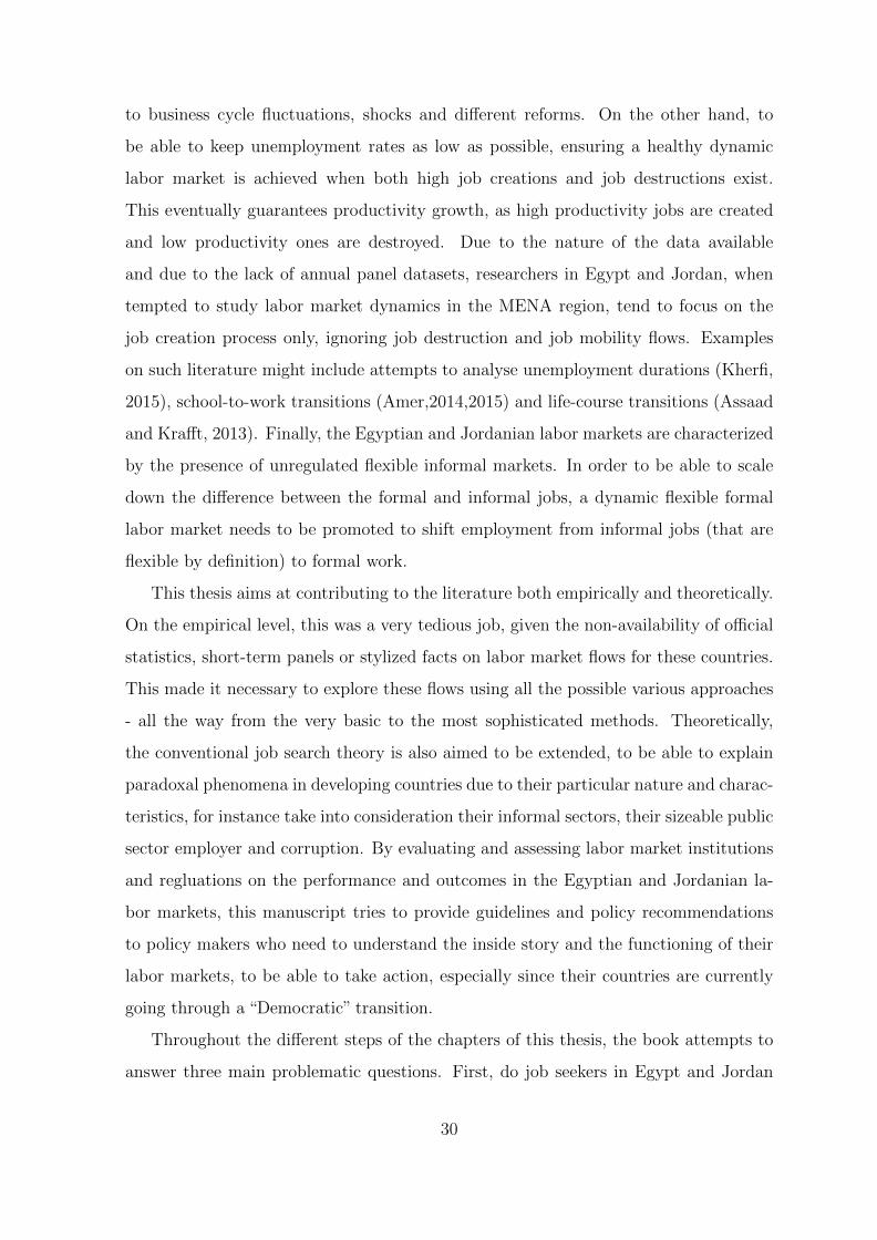
to business cycle fluctuations, shocks and different reforms. On the other hand, to

be able to keep unemployment rates as low as possible, ensuring a healthy dynamic

labor market is achieved when both high job creations and job destructions exist.

This eventually guarantees productivity growth, as high productivity jobs are created

and low productivity ones are destroyed. Due to the nature of the data available

and due to the lack of annual panel datasets, researchers in Egypt and Jordan, when

tempted to study labor market dynamics in the MENA region, tend to focus on the

job creation process only, ignoring job destruction and job mobility flows. Examples

on such literature might include attempts to analyse unemployment durations (Kherfi,

2015), school-to-work transitions (Amer,2014,2015) and life-course transitions (Assaad

and Krafft, 2013). Finally, the Egyptian and Jordanian labor markets are characterized

by the presence of unregulated flexible informal markets. In order to be able to scale

down the difference between the formal and informal jobs, a dynamic flexible formal

labor market needs to be promoted to shift employment from informal jobs (that are

flexible by definition) to formal work.

This thesis aims at contributing to the literature both empirically and theoretically.

On the empirical level, this was a very tedious job, given the non-availability of official

statistics, short-term panels or stylized facts on labor market flows for these countries.

This made it necessary to explore these flows using all the possible various approaches

- all the way from the very basic to the most sophisticated methods. Theoretically,

the conventional job search theory is also aimed to be extended, to be able to explain

paradoxal phenomena in developing countries due to their particular nature and charac-

teristics, for instance take into consideration their informal sectors, their sizeable public

sector employer and corruption. By evaluating and assessing labor market institutions

and regluations on the performance and outcomes in the Egyptian and Jordanian la-

bor markets, this manuscript tries to provide guidelines and policy recommendations

to policy makers who need to understand the inside story and the functioning of their

labor markets, to be able to take action, especially since their countries are currently

going through a “Democratic” transition.

Throughout the different steps of the chapters of this thesis, the book attempts to

answer three main problematic questions. First, do job seekers in Egypt and Jordan

30

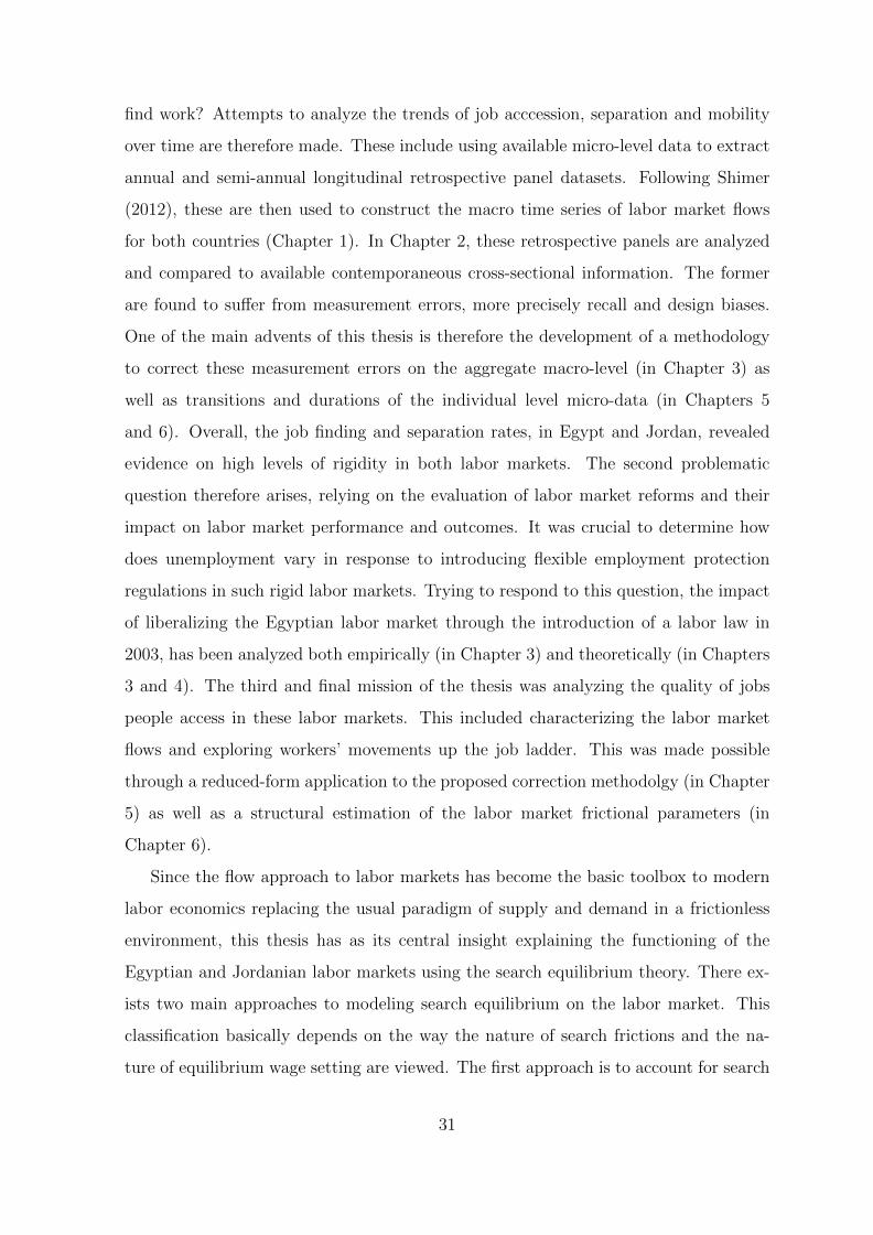
find work? Attempts to analyze the trends of job acccession, separation and mobility

over time are therefore made. These include using available micro-level data to extract

annual and semi-annual longitudinal retrospective panel datasets. Following Shimer

(2012), these are then used to construct the macro time series of labor market flows

for both countries (Chapter 1). In Chapter 2, these retrospective panels are analyzed

and compared to available contemporaneous cross-sectional information. The former

are found to suffer from measurement errors, more precisely recall and design biases.

One of the main advents of this thesis is therefore the development of a methodology

to correct these measurement errors on the aggregate macro-level (in Chapter 3) as

well as transitions and durations of the individual level micro-data (in Chapters 5

and 6). Overall, the job finding and separation rates, in Egypt and Jordan, revealed

evidence on high levels of rigidity in both labor markets. The second problematic

question therefore arises, relying on the evaluation of labor market reforms and their

impact on labor market performance and outcomes. It was crucial to determine how

does unemployment vary in response to introducing flexible employment protection

regulations in such rigid labor markets. Trying to respond to this question, the impact

of liberalizing the Egyptian labor market through the introduction of a labor law in

2003, has been analyzed both empirically (in Chapter 3) and theoretically (in Chapters

3 and 4). The third and final mission of the thesis was analyzing the quality of jobs

people access in these labor markets. This included characterizing the labor market

flows and exploring workers’ movements up the job ladder. This was made possible

through a reduced-form application to the proposed correction methodolgy (in Chapter

5) as well as a structural estimation of the labor market frictional parameters (in

Chapter 6).

Since the flow approach to labor markets has become the basic toolbox to modern

labor economics replacing the usual paradigm of supply and demand in a frictionless

environment, this thesis has as its central insight explaining the functioning of the

Egyptian and Jordanian labor markets using the search equilibrium theory. There ex-

ists two main approaches to modeling search equilibrium on the labor market. This

classification basically depends on the way the nature of search frictions and the na-

ture of equilibrium wage setting are viewed. The first approach is to account for search

31

frictions in the form of incomplete information about the available vacancies, which

generates a time delay until the matching between the unemployed workers and firms

with vacancies takes place. Diamond (1982), Mortensen (1982) and Pissarides (1985)

adopted this approach. Wages are determined in this case through a Nash bargaining

process as long as the application of the Nash solution to the equilibrium wage deter-

mination is justified (Binmore, Rubinstein, and Wolinsky, 1986). The second class of

models assumes that search frictions result from workers’ incomplete information about

the offered wages. In this case workers receive take-it or leave-it wage offers (one per

period) and have the choice to either accept or reject the offer before they can draw

a new one. Early job search models adopted this approach that was added later on

to the search equilibrium framework by Diamond (1971), Albrecht and Axell (1984)

and Burdett and Mortensen (1998). Wages are hence determined in these models via

a wage posting game among employers.

Assessing the inflows and outflows of unemployment becomes possible using the

first approach where the transition rates can be obtained in function of labor market

tightness, workers’ search intensities..etc (Pissarides, 1990). Chapters 3 and 4 therefore

choose to adopt this approach in an attempt to understand the nature of the dynamics

of the Egyptian labor market, in terms of whether workers find jobs or not and how

jobs are destroyed. This method however does not allow to portray the quality of

jobs and movements of workers up the job ladder since it is less informative about on-

the-job search and no endogenous wage offer distributions can be obtained. Empirical

applications are consequently very limited using the first approach. In contrast, the

second approach adopts a model with wage posting and on-the-job search which solves

for a unique endogenous wage offer distribution which is a crucial feature that facilitates

the estimation and the empirical application of the model. In an attempt to cover all

the methods, Chapter 6 therefore chooses to focus on the second class of models.

The rest of this thesis manuscript is divided as follows. Chapter 1 serves as an

introductory chapter, of which the primary objective is to describe the main develop-

ments in, and establish a number of key facts and descriptives about the recent history

of these important Egyptian and Jordanian labor market flows. The chapter provides

the main guidelines to how semi-annual and annual longitudinal retrospective panels

32

are extracted for Egypt and Jordan using the available Labor Market Panel Surveys

(ELMPS and JLMPS), which are to be used through out the thesis. The chapter also

provides a summary of the two countries’ institutional frameworks. It examines the

descriptive statistics of the labor market flows showing the similarities and differences

between the two countries. Overall, tThe findings of this chapter on the dynamics of

the Egyptian and Jordanian labor markets are not re-assuring. These show that job

accession and separation rates are extremely low in both economies, and even job-to-

job transitions do take place mainly in the informal sectors with the possibility that

people might be experiencing worsening job statuses rather than becoming more pro-

ductive and moving up the job ladders. The Jordanian labor market appear to be

relatively more mobile and flexible than the Egyptian labor market. However, with

no big differences between the job finding rates in the Jordanian formal and informal

sectors, the figures and patterns observed suggest that the Jordanian labor market is

more segmented than the Egyptian.

Previous literature such as Artola and Bell (2001), Bound, Brown, and Mathiowetz

(2001), and Magnac and Visser (1999) show that retrospective data suffer from prob-

lems such as difficulties in recalling dates or even that certain events occurred at all.

Panel data, that is data that are collected contemporaneously at different points in time

for the same individual, avoid this problem but because they are collected at discrete

points in time, they only provide information at those points in time and not on the

course of events between those points (Blossfeld, Golsch, and Rohwer, 2012). These

are also likely to suffer from sample attrition and misclassification errors (Artola and

Bell, 2001). In Chapter 2, due to these potential problems with both retrospective

and panel data, it becomes worthwhile to compare results on basic indicators related

to labor market dynamics from retrospective and contemporaneous panel data on the

same sample of individuals, in order to determine the conditions under which they

provide similar or substantially different results. To date, no study has undertaken

such a comparison in the MENA region. This chapter therefore takes advantage of

a unique opportunity to undertake such a comparison, where both panel and retro-

spective data are available for the same individuals in the Egypt Labor Market Panel

Survey (ELMPS) using 1998, 2006 and 2012 waves. Not only do the reference periods

33

of the retrospective data of each wave overlap with the dates of the previous waves

of the survey, allowing for comparisons of retrospective and panel data at the same

point in time, but the retrospective periods from different waves of the survey overlap

with each other as well, allowing for comparison of past events in one wave with the

same events as captured in another wave. In countries, where data collection budgets

represent a big issue, this chapter therefore tries to demonstrate whether it is possible

to collect information about labor market dynamics using retrospective data or is recall

error so great as to make panel data the only viable option. Findings show that it is

possible although caution is required on the type of information concluded from the

analysis and the level of detail used in the analysis (for instance differentiation between

very detailed categories such as self-employed and employers or regular and irregular

workers might be mis-leading). Past employment spells from retrospective data are

shown to be fairly reliable so long no fine distinctions between employment states are

made. Interspersed non-employment spells (unemployment and out-of labor force) be-

tween employment spells are however hard to recall. Retrospective questions eliciting

monetary amounts proved to be unreliable. Respondents tend to inflate the amount to

their equivalent value at the time of the survey. This chapter also provides guidelines

and lessons on how to use existing retrospective data from the ELMPS or other similar

surveys.

After having discussed the data and its issues in the first part, the second part of

this thesis is dedicated to evaluating the impact of introducing flexible employment

protection regulations on unemployment rates in developing countries. This becomes

possible in chapter 3 which proposes to evaluate an Egyptian labor market law which

was introduced in 2003, aiming to enhance the flexibility of the hiring and firing pro-

cesses. In general, only one earlier study by Wahba (2009) investigated the short term

impact (i.e after two years) of the law but on the formalization process in Egypt. The

Egypt labor market panel surveys (ELMPS 2006 and ELMPS 2012) are used to mea-

sure the impact of this reform on the dynamics of separation and job finding rates, and

to quantify their contributions to overall unemployment variability. Using extracted

longitudinal retrospective panel datasets created from the retrospective accounts of the

2006 and 2012 cross-sections and by overlapping the two surveys, the chapter estimates

34

annual and semi-annual transition probabilities of workers among employment, unem-

ployment and inactivity labor market states. A unique novel model is built to correct

for the recall and design bias observed in the aggregate labor market transitions ob-

tained from retrospective data. Using the ”corrected” data , it is then shown that the

reform increases significantly the separation rates in Egypt but leads to non-significant

effects on the job finding rates. The combined net effect is therefore an increase in the

levels of the Egyptian unemployment rate: separations increase whereas hirings remain

unchanged. This partial failure of the liberalization of the Egyptian labor market is

then explained theoretically by an increase in the set-up costs, interpreted as a capture

by the corrupt agent of the new surplus, in the Mortensen and Pissarides (1994) model.

Chapter 4 takes the analysis to a further step and attempts to explain to what extent

the Mortensen and Pissarides (1994) model is applicable to developing countries, such

as Egypt, where big shares of their employment lies in the informal and public sectors.

Limiting the analysis, as previous traditional literature, to only an unsegmented or

segmented Private labor market might be insufficient or might fail to explain the inside

story of the underlying different transitions and the particular nature of the MENA re-

gion labor markets. While recent attempts tried to include within the job search model

an informal sector (such as Albrecht, Navarro, and Vroman (2009), Meghir, Narita, and

Robin (2012), Bosch and Esteban-Pretel (2012), Charlot, Malherbet, and Ulus (2013,

2014) and Charlot, Malherbet, and Terra (2015)) or a public sector and an unsegmented

private sector (Burdett (2012) , Bradley, Postel-Vinay, and Turon (2013)), Chapter 4

aims to add both an informal and a public sector to the conventional Mortensen and

Pissarides (1994) model. A worker’s employment/non-employment choices are there-

fore based on the comparisons between his/her expected job values in the current or

all prospective jobs i.e in any of the three employment sectors. The model built in

this paper also takes into consideration fiscal realities faced by the public sector. It’s

true that the public sector can increase its wages but given its budgetary constraint,

it is likely to decrease the rate at which it hires employees. This could be done, as in

Egypt for instance, by rationing public sector vacancies. This chapter therefore makes

it possible to offer another explanation to the empirical paradox observed in chapter3

following the introduction of flexible employment protection in Egypt. Even though

35

the policy is directed to the formal private sector, it surely affects the interaction and

the flow of workers between the different employment sectors. Using qualitative ana-

lytics, the model is calibrated and simulations for the impact of the structural reforms,

particularly the Egypt Labor Law implemented in 2004, are provided. Supporting

evidence from available data on flows in Egypt between the employment sectors and

unemployment, before and after the 2004 reform are also shown. The main findings

suggest that introducing flexible employment protection rules, modelled as reduced fir-

ing taxes, favors job creation and job destruction in the private formal sector which

is the main aim of the policy. It increases job separations in the informal sector and

decreases workers finding informal jobs. Indeed, it is shown that the liberalization of

the labor market plays against the informal employment by increasing the profitability

of the formal jobs. But, if at the same time, the wages offered by the public sector

are increased,as what happened in Egypt (Said, 2015), this would create a crowding

out effect, where the new surpluses created by the labor market reform are more than

compensated by the new costs of worker mobility induced by the increase in the attrac-

tiveness of the public sector. This result is robust, even if the introduction of reduced

firing taxes decreases the proportion of on-the job search towards the public sector of

both workers in the formal and informal sectors.

The last part of the thesis aims at characterizing the labor market flows in the

Egyptian and Jordanian markets by exploiting the micro-level information available

in the data. Since as has been discussed earlier, the data suffers from measurement

errors, Chapter 5 serves as a methodological applied econometrics section that building

on the macro model developped in Chapter 3, it proposes a method to correct the

data on the individual transaction level (i.e. micro level). It creates user-friendly

weights that can be readily used by researchers relying on the ELMPS and JLMPS

retrospective panels. It is suggested that it is sufficient to match the retrospective

moments with true unbiased population moments, from auxiliary information such as

contemporaneous information from other waves of the same survey, or even external

data sources, so long comparability between the varaibles’ definitions is verified. As

a measurement error is estimates, this can be then distributed among the sample’s

individual observations/transactions in the form of micro-data weights. The chapter

36

proposes two types of weights: naive proportional weights and differentiated predicted

weights. The chapter shows that naive proportional weights offer the advantage of being

simple to calculate and handy. However, since retrospective panels are not random,

the predicted differentaiated weights attempt to re-obtain random samples within these

panels. This is mainly based in the assumption that if the individual is more probable

to transit, then he is more probable to mis-report. Both transaction-level weights i.e.

for each transition at a certain point in time, as well as panel weights i.e. for an entire

spell are created. The effect of these weights is shown significant through an application

using these weights. The determinants of labor market transitions are analyzed via

a multinomial regression analysis with and without the weights. The impact of these

weights on the regressions estimations and coefficients is therefore examined and shown

significant among the different labor market transitions, particularly separations.

Finally Chapter 6 uses a rudimentary partial equilibrium job search model a la

(Burdett and Mortensen, 1998) to estimate the structural labor market transitions

between employment and non-employment states in Egypt and Jordan, exploiting the

corrected extracted longitudinal retrospective panels obtained from 6-year panels using

retrospective information available in the Egypt labor market panel suvey (ELMPS)

fielded in 2012 and the Jordan labor market panel survey (JLMPS) fielded in 2010. The

chapter uses the close correspondance between the determinants of labor turnover and

wage mobility, and the determinants of the cross-sectional wage distribution, as per

Jolivet, Postel-Vinay, and Robin (2006) to be able to exploit the datasets available for

the countries in question, (i) to provide a quantitative measure of the search frictions

and (ii) to test to what extent the model fits the data i.e. reality and the particular

nature of these developing countries’ labor markets. The analysis adopts Bontemps,

Robin, and Van den Berg (2000) two-step semi-parametric estimation procedure. The

estimations are carried out using maximum likelihood techniques delivering frictional

transition parameters for each country, for the samples with and without longitudianl

correcting panel weights, as well as for two different age groups.The chapter shows

that correcting for the recall and design bias in the used datasets matters significantly

to the estimation of the job destruction parameters. The estimates of the index of

search frictions is as a result sensitive to this correction. The frictional parameters

37

in both countries are generally very low reflecting the rigidity of these labor markets.

Findings also show that in general the Jordanian labor market is more flexible than

the Egyptian, especially among the younger group of workers, where job durations are

relatively shorter. In contrast, Egyptian young workers have shorter non-employment

spells. In Egypt, the duration of remaining non-employed declines with age. In Jordan,

however, non-employment durations get shorter for the old group of workers and are

shorter than that for the Egyptian old workers. Young Egyptian workers are found to

have the highest level of search frictions, relative to the older Egyptian workers and

Jordanian workeres -both young and old. This implies that the firms’ monopsony power

in this trench of the Egyptian market is the highest leading to low levels of salaries.

Since small firms tend to pay lower wages, a higher density of small sized firms is

captured for the Egyptian market. This result is confirmed by the empirical data.

38

References

Albrecht, J., L. Navarro, and S. Vroman (2009): “The Effects of Labour Market

Policies in an Economy with an Informal Sector*,” The Economic Journal, 119(539),

1105–1129.

Albrecht, J. W., and B. Axell (1984): “An equilibrium model of search unem-

ployment,” The Journal of Political Economy, pp. 824–840.

Amer, M. (2014): “The School-to-Work Transition of Jordanian Youth,” in The Jor-

danian Labor Market in the New Millenium, pp. 64–104. Oxford University Press.

(2015): “Patterns of Labor Market Insertion in Egypt 1998–2012,” in The

Egyptian labor market in an era of revolution, pp. 70–89. Oxford University Press.

Artola, C., and U.-L. Bell (2001): “Identifying labour market dynamics using

labour force survey data,” .

Assaad, R., and C. Krafft (2013): “The Egypt labor market panel survey: intro-

ducing the 2012 round,” IZA Journal of Labor & Development, 2(1), 8.

Binmore, K., A. Rubinstein, and A. Wolinsky (1986): “The Nash bargaining

solution in economic modelling,” The RAND Journal of Economics, pp. 176–188.

Blossfeld, H.-P., K. Golsch, and G. Rohwer (2012): Event history analysis

with Stata. Psychology Press.

Bontemps, C., J.-M. Robin, and G. J. Van den Berg (2000): “Equilibrium search

with continuous productivity dispersion: Theory and nonparametric estimation,”

International Economic Review, pp. 305–358.

39

Bosch, M., and J. Esteban-Pretel (2012): “Job creation and job destruction in

the presence of informal markets,” Journal of Development Economics, 98(2), 270–

286.

Bound, J., C. Brown, and N. Mathiowetz (2001): “Measurement error in survey

data,” Handbook of econometrics, 5, 3705–3843.

Bradley, J., F. Postel-Vinay, and H. Turon (2013): “Public sector wage policy

and labor market equilibrium: a structural model,” Unpublished manuscript, 2, 14.

Burdett, K. (2012): “Towards a theory of the labor market with a public sector,”

Labour Economics, 19(1), 68–75.

Burdett, K., and D. T. Mortensen (1998): “Wage differentials, employer size,

and unemployment,” International Economic Review, pp. 257–273.

Charlot, O., F. Malherbet, and C. Terra (2015): “Informality in develop-

ing economies: Regulation and fiscal policies,” Journal of Economic Dynamics and

Control, 51, 1–27.

Charlot, O., F. Malherbet, and M. Ulus (2013): “Efficiency in a search and

matching economy with a competitive informal sector,” Economics Letters, 118(1),

192–194.

(2014): “Unemployment compensation and the allocation of labor in develop-

ing countries,” Journal of Public Economic Theory.

Diamond, P. A. (1971): “A model of price adjustment,” Journal of economic theory,

3(2), 156–168.

(1982): “Wage determination and efficiency in search equilibrium,”The Review

of Economic Studies, 49(2), 217–227.

Jolivet, G., F. Postel-Vinay, and J.-M. Robin (2006): “The empirical content

of the job search model: Labor mobility and wage distributions in Europe and the

US,” European Economic Review, 50(4), 877–907.

40

Kherfi, S. (2015): “Determinants of Unemployment Duration,” in The Egyptian labor

market in an era of revolution, pp. 90–107. Oxford University Press.

Klugman, J. (2010): “Human Development Report 2010–20th Anniversary Edition.

The Real Wealth of Nations: Pathways to Human Development,” .

Magnac, T., and M. Visser (1999): “Transition models with measurement errors,”

Review of Economics and Statistics, 81(3), 466–474.

Meghir, C., R. Narita, and J.-M. Robin (2012): “Wages and informality in

developing countries,” Discussion paper, National Bureau of Economic Research.

Mortensen, D. T. (1982): “The matching process as a noncooperative bargaining

game,” in The economics of information and uncertainty, pp. 233–258. University of

Chicago Press.

Mortensen, D. T., and C. A. Pissarides (1994): “Job creation and job destruction

in the theory of unemployment,” The review of economic studies, 61(3), 397–415.

Pissarides, C. A. (1985): “Short-run equilibrium dynamics of unemployment, vacan-

cies, and real wages,” The American Economic Review, pp. 676–690.

(1990): Equilibrium unemployment theory. MIT press.

Said, M. (2015): “JWages and inequality in the Egyptian labor market in an era of

financial crisis and revolution,” Discussion paper, Economic Research Forum, Cairo.

Shimer, R. (2012): “Reassessing the ins and outs of unemployment,” Review of Eco-

nomic Dynamics, 15(2), 127–148.

Wahba, J. (2009): “The impact of Labor market reforms on informality in Egypt:

Gender and work in the MENA region,” Discussion paper, The Population Council

Working Papers, 3. 0.

41

Part I

Data and Descriptives

42

Chapter 1

Labor Market Flows: Facts from

Egypt and Jordan 1

1.1 Introduction

The issue of labor market dynamics is crucial and central to understanding how they

function and how they create more and better jobs. Previous traditional literature on

Middle East and North Africa (MENA) countries, where analyses relied on static and

aggregate approaches, as well as repeated cross-sections to view stocks and changes

in stocks, are severly limited. It’s true that via stocks, one is able to point out if an

individual occupies an informal type of work, is unemployed or is even out of the labor

force. However, what really matters and might be extremely problematic is how long an

individual stays in that state and what is likely to be the destination after leaving that

state. In most developing countries, especially the MENA region, the readily available

cross-sectional data allow to only capture the stocks or the changes in stocks, but not

the flows underlying these stocks.

The recent introduction of new waves of surveys in the region as well as new empir-

ical techniques has now made possible more profound and thorough dynamic research.

Researchers, demographers and policy makers became increasingly interested in under-

standing employment histories or the worker’s life course after schooling, with a focus

1This chapter is mainly based on the paper“Job accession, separation and mobility in the Egyptianlabor market over the past decade” (Yassine, 2015).

43

on events, their sequence, ordering and transitions that people make from one labor

market state to another. Since the Arab Spring, the MENA countries are continously

debating on how to respond to the economic crises and on how to provide more equi-

table opportunities through their labor markets. Consequently, policy-relevant research

on labor market dynamics becomes particularly valuable.

Given the availability of data, the research conducted in this thesis provides evi-

dence from two developing MENA arab countries, Egypt and Jordan. Previous research

on labor markets in Egypt and Jordan has paid close attention to the stocks of the em-

ployed, the unemployed and the inactive (i.e., those not working or looking for work), as

well as to the balance between labor demand and supply often referred to as“tightness”.

However, the labor market stocks and aggregate indicators are fundamentally driven by

the behaviour of flows between employment, unemployment and inactivity. Egyptian

and Jordanian labor market dynamics remain therefore an unexplored research topic

where even official statistics lack records of these flows, namely job accession (transi-

tions from non-employment to employment) , separation (transitions from employment

to non-employment) and mobility (job-to-job transitions).

An understanding of all the relevant flows is essential to the comprehension of la-

bor market dynamics and business cycle fluctuations. For policy makers, knowledge

of those facts can help improve the monitoring of business cycles, the detection of in-

flection (turning) points and the assessment of labor market tightness. To guarantee

productivity growth along with economic (GDP) growth, it is important to ensure a

healthy dynamic labor market where low productivity jobs are being destroyed, higher

productivity jobs are being created and existing jobs are getting more productive. Lib-

eralizing labor markets is also important in the case of developing countries to scale

down the difference between formal and informal jobs, that are flexible by definition

given that this a part of the economy that is not taxed or monitored by any form

of legal-institutional framework. This paper can hence be seen as a guideline to the

creation of a number of measures of dynamics from the Egyptian and Jordanian avail-

able datasets. It provides a summary of the two countries’ institutional frameworks.

The paper examines the descriptive statistics of the labor market flows showing the

similarities and differences between the two countries.

44

The preliminary results of this paper are not reassuring in terms of the dynamics of

the Egyptian and Jordanian labor markets where job accession and separation seem to

be extremely low in the economy, and even job-to-job transitions do take place mainly in

the informal sectors with the possibility that people might be experiencing worsening

job statuses rather than becoming more productive and moving up the job ladders.

The Jordanian labor market appear to be relatively more mobile and more flexible

than the Egyptian labor market. With no big differences between the job finding rates

in the formal and informal sectors in Jordan, the figures and patterns observed suggest

that the Jordanian labor market is more segmented than the Egyptian market though.

Overall, the key answer to a healthy and dynamic labor market is simply firms and

workers becoming better at what they do, and for this to take place, policies in these

countries should encourage in the formal private sector all three types of transitions:

job accession, separation and mobility.

To the best of my knowledge, this paper is the first attempt to assess from a descrip-

tive point of view the transitions within/between employment and non-employment

states in the Egyptian and Jordanian labor markets. Discussions and debates in the

region’s seminars suggest that these labor markets are very rigid, where a worker can

spend his entire working lifetime in only one job. There is a need however to assess

such claims with concrete descriptive evidence, using recent panels and datasets, which

shall be the mission of this paper.

Thus the objective of this paper is to describe the main developments in, and

establish a number of key facts and descriptives about the recent history of these

important Egyptian and Jordanian labor market flows. The paper points out the

characteristics of labor market transitions, stayers and movers among the different

labor market states, and explores the key determinants to move, leave or quit a job.

The analysis tries to highlight remarks, if any, particularly for Egypt, on the period

after the January 2011 Uprising, after which it has been claimed that many workers

lost their jobs.

In this paper, both semi-annual and annual longitudinal retrospective panels over

the period 1998-2012 for Egypt and 1996-2010 for Jordan are extracted. This is done

by combining information obtained from retrospective job histories, unemployment

45

spells, a life events calendar (when available) and current job status details available in

the Egypt and Jordan Labor Market Panel Surveys (ELMPS and JLMPS respectively).

The innovation of obtaining an employment/non-employment vector for each and every

individual every six months over a period of ten years (for each country) allows to

monitor the fullest possible range of job accession, separation or job-to-job transitions

occurring in the Egyptian and Jordanian labor market during the observed period.

I am therefore able to quantify and characterize these transitions and hence provide

the literature with stylized facts and descriptives about Egyptian and Jordanian labor

market dynamics that even official statistics have lacked.

The rest of the paper is divided as follows. The second section surveys previous

literature on the evolution of the institutional framework of the Egyptian and Jordanian

labor markets. The third section briefly presents the structure of the questionnaires

and the data used in the analysis, the creation of semi-annual longitudinal retrospective

panels, and the resulting potential errors. The fourth section provides an overview of

the average gross flows of jobs and the macroeconomic labor market trends in Egypt.

The fifth section explores the characteristics of job leavers/losers and movers as opposed

to job stayers. Section 6 concludes.

1.2 Stylized Facts About Labor Markets in Egypt

and Jordan

Egypt and Jordan are two arab MENA labor markets which share certain common

characteristics with their neighboring arab countries. In general, these are countries

that are characterized by oversized public sectors, high rates of youth unemployment,

very weak formal private sectors and high shares of informality. The educational level

of the labor supply in these countries is rapidly growing on the one hand but highly

distorted on the other (Assaad, 2014a). It has also been well established that these

are countries with stagnant low female labor force participation rates when compared

to other regions. This section surveys the stylized facts and indicators provided by

previous literature, not only showing the key features of these two labor markets but

even showing more evidence to how it is crucial to study the flows driving their stocks.

46

Showing evidence from Gatti, Morgandi, Grun, Brodmann, Angel-Urdinola, and

Moreno (2013) in figure 1.1, Assaad (2014a) shows that the public sector constitutes

high shares of employment in arab countries as opposed to countries, either developing

or developed in other regions. Jordan is at the lead of these arab countries where on

average 40% of employment in the 2000’s has been concentrated in the public sector.

Egypt, on the other hand, has been experiencing a relatively retreating share of public

sector in employment which reached 25% in the 2000’s. This however has not always

been the case. In the 70’s and 80’s, all industrial employment was virtually public

sector and heavily unionized. The crisis of the beginning of the 90’s, compelled the

government however to look to the International Monetary Fund (IMF), World Bank

and the Paris Club for support, and that was when Egypt was required to undergo

a structural adjustment package as a counterpart to receiving a stand-by credit. The

result was an increase in economic activity, and a relatively stronger growth in the

private-sector since then.

Figure 1.1: Employment shares in the public sector (%), averages in the 2000s.

Source: Assaad (2014a) based on Gatti, Morgandi, Grun, Brodmann, Angel-Urdinola, and Moreno(2013)

Assaad (2014a) argues in his paper that the public employment in the arab countries

constitute an important share of the employment of politically significant groups such

as the educated middle class (which is mainly the case of Egypt and Jordan), citizens

of oil monarchies, and members of key sects, tribes or ethnic groups. These are also

authoritarian regimes that sort of offer implicit deals to these polically significant groups

as in to provide them with such stable well-compensated jobs in the bureaucracy or

47

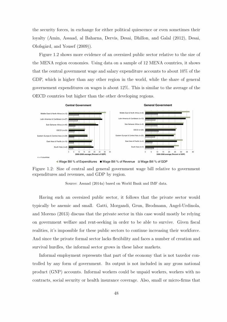
the security forces, in exchange for either political quiescence or even sometimes their

loyalty (Amin, Assaad, al Baharna, Dervis, Desai, Dhillon, and Galal (2012), Desai,

Olofsgard, and Yousef (2009)).

Figure 1.2 shows more evidence of an oversized public sector relative to the size of

the MENA region economies. Using data on a sample of 12 MENA countries, it shows

that the central government wage and salary expenditure accounts to about 10% of the

GDP, which is higher than any other region in the world, while the share of general

governement expenditures on wages is about 12%. This is similar to the average of the

OECD countries but higher than the other developing regions.

Central Government

0 5 10 15 20 25 30 35 40

South Asia (n=8)

East Asia & Pacific (n=10)

Eastern Europe & Central Asia (n=28)

OECD (n=24)

Sub-Saharan Africa (n=45)

Latin America & Caribbean (n=27)

Middle East & North Africa (n=12)

2000-2008 average (Percent of GDP)

General Government

0 5 10 15 20 25 30 35 40

South Asia (n=4)

East Asia & Pacific (n=4)

Eastern Europe & Central Asia (n=25)

OECD (n=25)

Sub-Saharan Africa (n=9)

Latin America & Caribbean (n=13)

Middle East & North Africa (n=6)

2000-2008 average (Percent of GDP)

Wage Bill % of Expenditures Wage Bill % of Revenue Wage Bill % of GDP

n = # countries

Figure 1.2: Size of central and general government wage bill relative to governmentexpenditures and revenues, and GDP by region.

Source: Assaad (2014a) based on World Bank and IMF data.

Having such an oversized public sector, it follows that the private sector would

typically be anemic and small. Gatti, Morgandi, Grun, Brodmann, Angel-Urdinola,

and Moreno (2013) discuss that the private sector in this case would mostly be relying

on government welfare and rent-seeking in order to be able to survive. Given fiscal

realities, it’s impossible for these public sectors to continue increasing their workforce.

And since the private formal sector lacks flexibility and faces a number of creation and

survival hurdles, the informal sector grows in these labor markets.

Informal employment represents that part of the economy that is not taxedor con-

trolled by any form of government. Its output is not included in any gross national

product (GNP) accounts. Informal workers could be unpaid workers, workers with no

contracts, social security or health insurance coverage. Also, small or micro-firms that

48

operate outside the regulatory framework, and formal(small or large) registered firms

that partially evade taxes and social security contributions might be considered infor-

mal. The literature uses three main measures of informality (1) the Schneider Index

(Schneider, Buehn, and Montenegro, 2010) which uses a broad set of country correlates

to estimate the share of production not declared to tax and regulatory authorities, (2)

the share of employed workers without social security coverage, and (3) the prevalence

of self-employment.

Figure 1.3 shows that a typical non-GCC MENA country produces about 28% of

its GDP and employs 65% of its labor force informally. It also shows how the MENA

region ranks using the different informality definitions, among the other regions of the

world both developped and developing regions. The question becomes where do Egypt

and Jordan rank among these MENA countries. In figure 1.4, it is obvious that while

Egypt is below the MENA region median of employing workers informally, it produces

35% of its output in the shadow economy. As for Jordan, it employs like a typical

median MENA country about 61% of its labor force informally and its undeclared

output amounts to 20% of its GDP (slightly below the MENA median). In order

to be able to capture the vulnerability of employment as a result of informality, the

analysis throughout this thesis relies on the first definition of informality, i.e. the lack

of contribution to social security. The data used relies, as will be discussed in the

next section, on labor market surveys. The individuals are asked if they are employed

whether they have (1) an official registered contract with the employer and (2) social

insurance. Based on a positive response to any of these two questions, an individual is

categorized as formally employed.

The above structure of the labor market gives a sense of the framework of the labor

markets in the two countries in question, namely Egypt and Jordan. It’s important

to recall at this point that the MENA region where these countries belong displays on

average low levels of employment and high levels of unemployment in comparison to

other regions of the world (Gatti, Angel-Urdinola, Silva, and Bodor, 2014).

Another important point that the reader has to keep in mind all throughout the

analysis conducted in this thesis is the differences in the labor law regulations of these

two countries. Contextualizing the analysis according to the labor market regulations

49

of each country is crucial in order to be able to build robust conclusions about their

labor market dynamics outcomes.

The legal framework in Jordan is mainly comprised of the Jordanian Labour Law

(8) of the year 1996 and its amendments. This regulates the relationship between the

Employer and the Employee. In this law, two types of contracts are considered; definite

duration contracts and indefinite durations contracts. The termination of the contract

without legitimate and adequate justification is possible, so long either party shall

compensate the other for the harm incurred. The contract of employment terminates

at the expiry of a fixed-term contract or at the completion of the task for which the

contract was concluded. The contract is considered renewed if both parties continue to

abide to the contract after its expiry. This legal framework for employment contracts

in Jordan has been applied since 1996. However in Egypt, the definite duration type

of contracts and the right of an employer to terminate an employee has only been

introduced via the 2003 Egypt Labor Law (12), which was implemented in 2004. Before

2004, workers were at some sort appointed for their entire working lifetime in the private

sector. The employer had very weak rights to terminate employers or to put end to

their contracts. It’s important however to note that the 2004 law regulations were only

applied to those who accessed jobs and signed their contracts after 2004. Having said

that, one can conclude that the Jordanian government has been trying to liberalize its

labor market way before the Egyptian.

50

Figure 1.3: Informality in the MENA region Versus other world regions.

Source: Gatti, Angel-Urdinola, Silva, and Bodor (2014) based on Schneider, Buehn, and Montenegro(2010) and WDI data.Note: GCC: Gulf Co-operation Council, ECA: Europe and Central Asia, LAC: Latin America and theCaribbean, EAP: East Asia Pacific, SA: South Asia, SSA: Sub-Saharan Africa

51

Figure 1.4: Informality in Egypt and Jordan versus a selected number of non-GCCMENA countries.

Source: Gatti, Angel-Urdinola, Silva, and Bodor (2014) based on Loayza and Wada (2010)

52

1.3 Methodology: From Stocks to Flows

1.3.1 Questionnaires

The analysis relies mainly on the Egypt Labor Market Panel Survey (ELMPS)

fielded in 2012 and the Jordan Labor Market Panel Survey (JLMPS) fielded in 2010.

The ElMPS 2012 is the third round of a periodic longitudinal survey that tracks the

labor market and demographic characteristics of households and individuals interviewed

in 2006 and 1998. The JLMPS 2010 is however the first round of the survey in Jordan.

A second round in 2016 is planned to track the same individuals that were interviewed

in the first wave. Both datasets are designed to be nationally representative.

The ELMPS 2012 has a total sample of 12,060 households and 49,186 individu-

als, who were interviewed. The JLMPS 2010 has a total sample of 5102 households

and 25,969 individuals. The questionnaires have similar structures with some minor

differences some of which will be discussed in the next paragraph.

The samples used in the analysis through out this thesis rely heavily on retrospec-

tive accounts available in both questionnaires. These are questions that apply to all

individuals who ever worked and who are above the age of 6. In the ELMPS 2012, these

retrospective questions were asked in a chronological order, starting at the first status

of the individual in the labor market or as he exits school (whichever is earlier) and

ending at the the fourth status (if needed). Individuals were also asked explicitly about

their status three months before the January 2011 Uprising in case it was not similar to

their current status at the time of the interview in 2012. For the JLMPS 2010 as well

as the ELMPS 2006 and 1998, the order of the statuses was reversed. Individuals were

asked about their current status2, their previous status and the previous-to-previous

status. It’s important to note that these statuses in both questionnaires can be em-

ployment, unemployment or inactivity states. For the JLMPS 2010, ELMPS 2006 and

ELMPS 1998, there was also an extra section to ask about the first job. Table 1.1

shows the list of questions asked for each of the above individual’s statuses, as well as

their responses’ codes .

2This usually coincides with the current status obtained from the current employment and unem-ployment chapters of the questionnaire. The latter chapters included much more detailed questionsabout the job and the unemployment spells though.

53

Date of start of the status (month and year)

Employment status1. waged employee 9. full time student2. employer 10. <15 years old and neither works nor studies *3. self employed 11. does not want work*4. unpaid working for family 12. retired (<65 years old) does not work and has no desire to work5. unpaid working for others 13. temporarily disabled6. unemployed worked before 14. Unpaid leave for a year or more7. new unemployed 15. more than 65 years old8. housewife 16. other

Occupation ( 6 digit - based on ISCO88)

Economic activity (4 digit - based on ISIC 4)

Inside Establishment/ In same or another Establishment/Out of Establishment1. Same establishment/ in establishment 2. Another establishment3. Outside establishment

Economic sector1. government 4. investment**2. public enterprise 5. foreign**3. private 6. non-profitable NGO**7. other including co-operatives

The size of the economic unit*1. 1 - 4 5. 50 - 992. 5 - 9 6. more than 1003. 10 - 24 7. don’t know, very large4. 25 - 49 8. don’t know

Job stability1. permanent 3. seasonal2. temporary 4. casual

Contract1. Yes, indefinte duration2. Yes, definite duration3. No ———-> 114. N.A ———–> 11Did you acquire this contract at the time you obtained your job?*1. Yes ———>12 2. NoWhen did you acquire this contract?* ————>12Did any other workers within your firm have a contract?*1. Yes 2. No 3. N.A.

Social security1. Yes 2. No ——> 15Did you acquire social security at the time you obtained your job?*1. Yes ——> 16 2. NoWhen did you acquire this social security?* ——>16Did any other workers within your firm have social security?*1. Yes 2. No

Work location

Reason for change from this status to the next status *1. terminated by the employer 4. Suspension of the project (employers and self- employed)2. Contract ended and not renewed by the employer 5. No change3. Quit volutarily/resigned 6. Other (Specify)

Table 1.1: Questions asked to individuals in the retrospective sections of the Egyptand Jordan Labor Market Panel Surveys

(*) These are questions/categories that are only available in the ELMPS2012.(**) The distinction between these three categories was not made in the JLMPS 2010. There was onlya category for co-operatives and a category for international organizations.

54

Exploiting the raw data from these retrospective accounts allows to extract a

worker’s lifetime trajectory every six months3 for only individuals who ever worked.

These showed when and for how long the individual has been employed, unemployed

or inactive in a certain spell. These semi-annual panels are then augmented by adding

in information from sections about current employment and current unemployment in

the questionnaires. These are large and detailed sections that include detailed ques-

tions on employment and unemployment detection over the past 7 days, all the job’s

and firm’s characteristics in terms of contracts, social insurance, stability, vacations

(in case of employment) and all unemployment search and reasons for not working

questions (in case of unemployment) 4. Finally, people who were never employed or

unemployed are added to the sample as inactives throughout the entire panel. It was

possible in the case of Egypt (ELMPS 2012) to cross validate the dates of start and

end of statuses/jobs, due to the availability of a life events’ calendar. This calendar

pointed out changes in and spells of employment, education, marriage and residence.

1.3.2 Definitions and Potential Problems

The available information on the individual’s career trajectory, not only allows to tell

if the individual is/was employed at some point in time, but also enables the detection

of the type of employment he/she occupied as well as some of the job’s characteristics.

Distinction is made in the analysis between public sector wage workers, private formal

wage workers, private informal wage workers and non-wage workers (including self-

employed, employers and unpaid workers).

As mentioned above, a worker is defined to be employed in a formal job if he or she

has a contract and/or social insurance. Only the ELMPS 2012 questionnaire makes it

possible to determine the formality of the firm where a firm is defined as formal when

the worker interviewed has a formal job or other workers in the firm have contracts

and/or social insurance. These are firms that partially evade taxes and social security

contributions. Questions about the firm’s formality are more detailed in the current

employment section; e.g. workers are asked explicitly whether their employer keeps

3It was impossible to draw these trajectories every month given the size of the samples and thehigh rate of missing observations obtained when asking about the month of start of the status.

4The full questionnaires are publicly available on the website http://www.erfdataportal.com

55

registers and accounting books or not. These are questions that are not asked in the

retrospective chapter.

The extra questions added to the ELMPS 2012 questionnaire about the time lag

between accessing a job and acquiring a contract or social insurance made it possible to

capture as fully as possible informal-to-formal job-to-job transitions that the individuals

have gone through during their work history. It is important to make this distinction

even if it is within the same job in the same firm. Not only that this allows to capture an

extra job-to-job transition, but also to detect for how long this employment has lasted

informally with no legal framework i.e. no government monitoring, no tax payment and

no contribution to the social security system. Moreover, assuming that an indiviual

was first employed informally in a job, which then became formalized and then later on

this indiviudal moved to the public sector. If one ignores the formalization of the job,

the final transition would be recorded as Informal → public, which does not actually

convey the true story. In reality, this individual moved from his job even though it

got formalized (i.e. a formal private sector job) to the public sector for some specific

reason. The motive behind a formal → public transition would definitely be different

than the motive of an informal → public transition.

Due to missing observations of the month of the start of a certain status, the ob-

served transitions were not realisticly distributed over the 2 semesters of each year.

The semi-annual transitions where therefore not representative for the size of these

transitions during a period of 6 months. In attempt to make use of the maximum pos-

sible information available in the surveys, two longitudinal retrospective panels were

extracted, one where the individuals are being followed every six months (i.e. semi-

annually) and the other where they are being followed annually. Stocks refer to and are

calculated based on a specific aggregate at the beginning of the year. These stocks are

therefore derived from the annual trajectories. For the transitions however (job acces-

sion, separation and switches), these are flows that occur during the year in question,

and since the aim is to capture the most possible number of transitions the inter-

viewed individuals went through during the year t, transitions are derived from the two

semestrial panels of year t and then aggregated to give the total number of transitions

observed in the year t.

56

Given the above steps adopted to create the longitudinal retrospective panels, the

final sample obtained from the raw data includes all individuals, 6 years and older, who

have ever worked in the Egyptian and Jordanian labor markets as well as the new labor

market entrants (i.e new unemployed) and individuals who have been permanently out

of the labor force. Throughout the rest of the thesis, different sub-samples are used

and hence are described in detail in the relevant section.

In general, using panel surveys may suffer from attrition bias, which is addressed

by using the attrition weights attributed in this dataset and which are used to expand

figures to the population level (Assaad and Krafft (2013)). These are referred to,

hereafter, by expansion weights.

Missing values about the month of start of a job tend to be problematic when

creating the longitudinal retrospective panels. A set of assumptions, when creating the

data sets, are therefore being adopted. In the survey, a status could not be recorded

unless an individual has spent at least 6 months in it. If the month values are missing

and two job statuses started in the same year, it is assumed that an individual has

spent the first half of the year in one job and the second in the other. If the month of

start of a job is missing and only one job status started in that year, I assume that the

status started at the begining of the year. If the year of start of the status was missing,

nothing could be done about this and the individual would have had to be dropped

from the sample. Fortunately enough, very few number of individuals had the last case

and the missing dates were mostly among the very old statuses. If one limits the panel

to the most recent 10 years for example, these missings should therefore not affect the

final sample.

Another potential type of measurement error the data is susceptible to is response

error. This includes recall error which I try to reduce by limiting the analysis to

the most recent years prior to the year of the survey i.e. not going too far back in

time. Response errors also include “present” mis-report bias, that is when some people

deliberately mis-report their current employment status and information, even though

they have given exact and correct information about their work history, just to avoid

57

taxes and government registers5. That both these types of error are occurring becomes

obvious when the analyses using ELMPS 2012 and ELMPS 2006 were overlapped and

when unemployment rates from stocks and flows were compared. Further research and

investigation are done in Assaad, Krafft, and Yassine (2015) (chapter 2) to explore

the extent of bias (whether recall or response) comparing longitudinal retrospective

panel data sets constructed using the retrospective questions and the available ELMPS

cross-sections 1998, 2006 and 2012.Langot and Yassine (2015) (chapter 3) proposes a

method to correct this bias.

The analysis is carried out over the period 1998-2012 for Egypt and 1996-2010 for

Jordan. Going back in time, the sample should have included people who were alive in

the past but passed away before 2012 and hence did not respond to the ELMPS. This

is defined as “backward attrition”. In an attempt to avoid this type of attrition, the

age of individuals in the sub-samples is limited to between 15 and 49 years old in year

t in the retrospective panel constructed prior to the year of the survey.

1.3.3 Concepts of Labor Market Dynamics 6

In this paper, the working age population at year t (Wt) comprises 3 stocks of

individuals; employed Et , unemployed Ut and inactive (out of the labor force) It.

Wt = Et + Ut + It (1.1)

The labor force Lt is made up of the employed and unemployed.

Lt = Et + Ut (1.2)

Total employment in year t+ 1 is determined by the employment in the previous year

t , the hiring flow from the pool of unemployed MUEt and inactive M IE

t , less the gross

5The ELMPS 2012 and JLMPS 2010 survey were conducted by the official National statisticaloffices’ personnel and hence for the interviewed households, it was government authorities collectingthe information.

6In this section, concepts discussed by Gomes (2012) and Shimer (2012) are summarized.

58

separation flows to unemployed and inactive respectively; SEUt and SEIt .7

Et+1 = Et +MUEt +M IE

t − SEUt − SEIt (1.3)

Similarly, the unemployment stock changes over time, however this time flows between

the unemployed and inactive stocks GUI and GIU are added.

Ut+1 = Ut −MUEt + SEUt −GUI

t +GIUt (1.4)

The empirical literature has studied labor market dynamics using different ap-

proaches. Emphasis has been put on gross flows in work Blanchard, Diamond, Hall,

and Murphy (1990) and Bleakley, Ferris, and Fuhrer (1999), and also on transition rates

like work by Shimer (2012) , Fujita and Ramey (2009) and Davis, Haltiwanger, and

Schuh (1996). Since this paper is a first attempt to explore facts and statistics about

the Egyptian and Jordanian labor market dynamics, the best would be to provide a

thorough survey of both approaches using the ELMPS 2012 and the JLMPS 2010. It

is extremely important to note that throughout the paper when talking about job ac-

cession, I differentiate between hiring rates h and job finding rates f . The hiring rate

measures the rate at which employment expands between two points in time calculating

new jobs created as a rate relative to the existing number of jobs. It resembles the job

creation rate discussed from the firm dynamics point of view (Davis, Haltiwanger, and

Schuh, 1996)8. The job finding rate represents the probability that a non-employed

individual finds a job (Shimer, 2012). To be able to understand this difference, it is

crucial at this point to distinguish between two concepts used in the analyses of labor

market dynamics; job turnover and labor turnover. The economy-wide job turnover

rate is simply the absolute sum of net employment changes across all establishments or

7The superscipts ij, where i 6= j, denote the origin state i (the state from which an invidual istransiting) and the destination state j ( the state to which an individual is transiting).

8This is what is referred to in the literature as job creation rate (in this analysis it does not includeunfilled vacancies, since estimates are obtained from an individual workers’ survey). This is usuallycalculated from individual firms’ level data. I therefore choose to call it hiring rate. It is also importantto note that the job turnover by definition does not include job vacancies that remain unfilled, whichexplains why the ELMPS synthetic panel data set can be used to calculate the Egyptian job turnover.

59

firms, expressed as a proportion of total employment. By simply comparing two points

in time, it is an indicator of the expansion or contraction of employment within estab-

lishments or firms in the economy. Labor turnover is simply the sum of job turnover

and the movement of workers into and out of ongoing jobs in establishments or firms.

Workers find and leave jobs regardless of whether the firm, or even employment in

the economy itself is growing or declining. For this reason, the analysis in this paper

distinguishes between the hiring rate (new jobs as a proportion of employment i.e. the

expansion of employment in the economy) and the job finding rate , which is simply the

probability an unemployed worker finds a job and moves into the stock of employed.

To summarize, the flows discussed in this paper, can be categorized into three types;

• Job Accession: when a non-employed individual (unemployed or inactive) gets

a job. This is described by the hiring and job finding rates.

• Job-to-Job Transitions: when an employed worker changes jobs (employers),

or changes formality status within the same job.

• Separation: when an employed worker exits his or her job. It is important to

note that this includes voluntary (quits) and involuntary (job loss) exits, which

will be discussed in detail below. 9

1.4 General Macroeconomic Trends

Labor market stocks and aggregate indicators are fundamentally driven by flows

between employment, unemployment and inactivity. This section discusses these flows

and their evolution over time as well as the characteristics of individuals who are at

risk of these transitions. The sample includes only male workers within the working

age population (between 15 and 64 years of age). Female workers are excluded from

the sample since transitions of female workers follow special patterns and are related

to different factors such as marriage, child-birth and sector of employment.

9For details about how the gross flows and transition rates are formalized in equations, see appendix1.A.

60

1.4.1 Average Gross Flows and Transition Probabilities over

the period 2002-2012 for Egypt and 2000-2010 for Jor-

dan

Figures 1.5, 1.6, 1.7 and 1.8 summarize the average annual gross worker flows for

males between 15 and 64 years of age over the periods 2000-2010 and 2002-2012 in

Jordan and Egypt respectively. These figures report the total (expanded) number of

people that changed status in thousands (t) and as a percentage of the working age

population (p) and as a transition rate out of the stock of employed workers (e).

According to the ELMPS data, over the period 2002-2006, there was an average

400,000 net increase in employment in Egypt every year whilst over 2007-2012 the

increase was 300,000. The JLMPS showed that over both periods 2000-2004 and 2005-

2010, the annual net employment increase in Jordan amounted to 20,000 jobs. Of course

substantial gross flows hide behind these values. An annual average of 190,000 Egyp-

tian male workers moved out of employment over the period 2000-2006, approximately

80% of whom moved into inactivity. Over the period 2007-2012, 290,000 Egyptian

workers per year moved out of employment, of whom about 70% to inactivity. In Jor-

dan, over the period 2000-2004, about 20,000 moved out of employment yearly, 50% of

them leaving the labor force. Over the period 2005-2010, the number of people leaving

employment every year increased to 35,000 and only 40% of them moved to inactivity.

During the first Egyptian sub-period (2002-2006), 590,000 male workers moved into

employment and over 2007-2012, it was 550,000, while in Jordan these transitions in-

creased from a yearly average of 43,000 during the first sub-period to a yearly average of

56,000 during the second. The majority of people transiting from non-employment to

employment, over both periods in Egypt, were entrants from inactivity, being 78% over

2002-2006 and 72% over 2007-2012.In Jordan, the share of entrants from inactivity in

transitions into employment was lower, being 62% over 2000-2004 and 44% over 2005-

2010. In general and in both countries, the percentage of the working age population

that moves out of employment into unemployment almost doubles between the two pe-

riods and increases slightly for employment-to-inactivity moves. Hiring from inactivity

(which is most likely new labor market entrants) slows down in both Egypt and Jordan.

61

Hiring slightly increases for workers entering the employed pool from unemployment

in Egypt but almost doubles in Jordan. The flows in these figures also show very low

transitions between unemployment and inactivity, which is normal and expected since

usually the frontiers between unemployment and inactivity are not perfectly defined.

This also mainly comes from the fact that the information obtained from the retrospec-

tive accounts of non-employment spells depend on the interpretation of the interviewer

and the interviewee of the definition of unemployment. As previously mentioned, the

retrospective section doesnot contain detailed unemployment detection questions as in

the case of the current status. Moreover, given the questionnaire’s structure, it is hard

to detect in case the individual has never worked if he has ever been unemployed in

the past. Unless, the never worked individual is currently unemployed, the data would

contain no record of unemployment spells for him/her.

It is also worth noting here that the values reported in this paper maybe inap-

propriate to compare with other countries’ estimates (with panel surveys of different

structures) due to the existence of multiple transitions. To avoid people reporting sum-

mer internships and very short-term type of jobs, the ELMPS 2012 and JLMPS 2010

questionnaires are only designed to capture a job status that has lasted for at least

6 months. Now, suppose someone is unemployed in the first month, then moves to

inactivity in the second, and then back to unemployment. While a monthly survey (as

in the case of many developed countries’ labor market data) would pick up all transi-

tions, the semi-annual synthetic panel would not detect any. It is possible to overcome

the problem of multiple transitions by correcting for time aggregation (as in Shimer

(2012)). For this to hold true, one has to assume that the conditional probabilities

are equal across monthly transitions that generate the observed semi-annual proba-

bilities. It is therefore impossible to make final conclusions about the rigidity of the

Egyptian and Jordanian labor market at this stage, not only because of the multiple

transitions problem but also given the recall error and other data problems discussed

in the previous section.

62

Employment 15,840(t) 80.8(p)

Unemployment 523(t) 2.7(p)

Inac;vity 3247(t) 16.6(p)

Into W.A.P E – 184 (t) U – 11 (t) I – 534 (t)

Out of W.A.P E – 51 (t) U – 1 (t) I – 44 (t)

37 (t) 0.19 (p) 125 (t)

0.64 (p) 461 (t) 2.35 (p) 8 (t)

0.04 (p)

117 (t) 0.60 (p)

154 (t) 0.79 (p)

519 (t) 2.65 (p)

(a) 2002-2006

Employment 17,960 (t) 79.99 (p)

Unemployment 643 (t) 2.86 (p)

Inac<vity 3,852 (t) 17.15 (p)

Into W.A.P E – 156 (t) U – 13 (t) I – 506 (t)

Out of W.A.P E – 74 (t) U – 2 (t) I – 64 (t)

88 (t) 0.39 (p) 149 (t)

0.66 (p) 400 (t) 1.78 (p)

6 (t) 0.02 (p)

103 (t) 0.46 (p)

201 (t) 0.89 (p)

733 (t) 3.26 (p)

(b) 2007-2012

Figure 1.5: Average annual gross flows, over the period 2002-2012, for Egyptian maleworkers between 15 & 64 years of age

W.A.P: working age populationp: percentage of working age populationt: thousandsSource: Author’s own calculations using ELMPS 2012. Yearly expanded and unexpanded number oftransitions are provided in the appendix 1.B.

Employment 15,840(t) 80.8(p)

Unemployment 523(t) 2.7(p)

Inac;vity 3247(t) 16.6(p)

0.23 (e) 0.79 (e) 2.91 (e)

0.05 (e)

0.74 (e)

0.97 (e)

3.27 (e)

(a) 2002-2006

Employment 17,960 (t) 79.99 (p)

Unemployment 643 (t) 2.86 (p)

Inac<vity 3,852 (t) 17.15 (p)

0.49 (e) 0.83 (e) 2.23 (e)

0.03 (e)

0.57 (e)

1.12 (e)

4.08 (e)

(b) 2007-2012

Figure 1.6: Average annual transitions (as a percentage of employment), over the period2002-2012, for Egyptian male workers between 15 & 64 years of age

e: transition rate out of stock of employedp: percentage of working age populationt: thousandsSource: Author’s own calculations using ELMPS 2012. Yearly expanded and unexpanded number oftransitions are provided in the appendix 1.B.

63

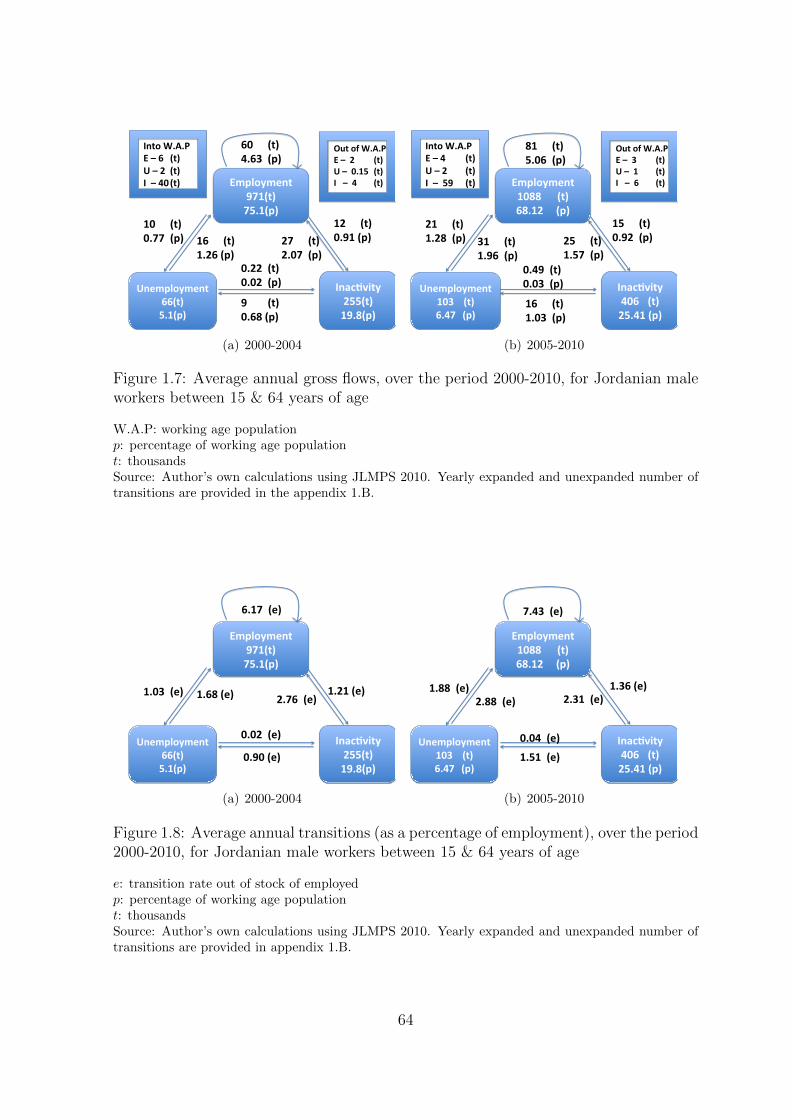
Employment 971(t) 75.1(p)

Unemployment 66(t) 5.1(p)

Inac7vity 255(t) 19.8(p)

Into W.A.P E – 6 (t) U – 2 (t) I – 40 (t)

Out of W.A.P E – 2 (t) U – 0.15 (t) I – 4 (t)

10 (t) 0.77 (p) 16 (t)

1.26 (p) 27 (t) 2.07 (p) 0.22 (t)

0.02 (p)

9 (t) 0.68 (p)

12 (t) 0.91 (p)

60 (t) 4.63 (p)

(a) 2000-2004

Employment 1088 (t) 68.12 (p)

Unemployment 103 (t) 6.47 (p)

Inac:vity 406 (t) 25.41 (p)

Into W.A.P E – 4 (t) U – 2 (t) I – 59 (t)

Out of W.A.P E – 3 (t) U – 1 (t) I – 6 (t)

21 (t) 1.28 (p) 31 (t)

1.96 (p) 25 (t) 1.57 (p)

0.49 (t) 0.03 (p)

16 (t) 1.03 (p)

15 (t) 0.92 (p)

81 (t) 5.06 (p)

(b) 2005-2010

Figure 1.7: Average annual gross flows, over the period 2000-2010, for Jordanian maleworkers between 15 & 64 years of age

W.A.P: working age populationp: percentage of working age populationt: thousandsSource: Author’s own calculations using JLMPS 2010. Yearly expanded and unexpanded number oftransitions are provided in the appendix 1.B.

Employment 971(t) 75.1(p)

Unemployment 66(t) 5.1(p)

Inac7vity 255(t) 19.8(p)

1.03 (e) 1.68 (e) 2.76 (e)

0.02 (e)

0.90 (e)

1.21 (e)

6.17 (e)

(a) 2000-2004

Employment 1088 (t) 68.12 (p)

Unemployment 103 (t) 6.47 (p)

Inac:vity 406 (t) 25.41 (p)

1.88 (e) 2.88 (e) 2.31 (e)

0.04 (e)

1.51 (e)

1.36 (e)

7.43 (e)

(b) 2005-2010

Figure 1.8: Average annual transitions (as a percentage of employment), over the period2000-2010, for Jordanian male workers between 15 & 64 years of age

e: transition rate out of stock of employedp: percentage of working age populationt: thousandsSource: Author’s own calculations using JLMPS 2010. Yearly expanded and unexpanded number oftransitions are provided in appendix 1.B.

64

1.4.2 Evolution of Labor Market Flows & Business Cycles

Figure 1.9 shows the evolution of hiring, separation and job-to-job transition rates

over the period 1998-2011 in Egypt and 1996-2010 in Jordan, for both male and female

workers. The figure also includes jobs created, jobs lost, and the GDP growth rate over

time. In Egypt, the trend of the aggregate job flows is relatively stable within the sample

over time. However, for male workers, there appears an inflection point at the year 2009.

It is a possibility that part of this abrupt change in trends observed, particularly in

both the job accession and separation rates, is a result of the downturn of the economy

after the financial crisis and the January 2011 Uprising. The following chapters however

show that this increase is mostly artificial and is driven by measurement errors in the

data (see Assaad, Krafft, and Yassine (2015) (chapter 2) and Langot and Yassine (2015)

(chapter 2)). This turning point in trends happens earlier for the Egyptian job-to-job

transition rates. Assaad, Krafft, and Yassine (2015) (chapter 2) show that conclusions

built on trends of job-to-job flows from retrospective data are relatively reliable. Levels

however can be underestimated. As for Jordan, the general trend of these job flows,

whether hiring, separation or job-to-job, is an increase over time. Separation and hiring

rates were stable or slightly increasing between 1996-2004, with a much steeper increase

afterwards especially for separtion rates between 2009-2010. The job-to-job and hiring

flows continue to increase up to 2009, where again a turning point is observed, dropping

the rates abruptly by 1 percentage point for the hiring and about 3 percentage points

for the job switches. The magnitude of these flows, for both males and females, is in

general higher than their counterparts in the Egyptian labor market. Even if these

trends or levels are partially artificial and biased, they provide preliminary evidence to

the Jordanian labor market being more flexible and mobile than the Egyptian.

In both countries, female workers have higher separation rates than their male

peers. They usually move out of employment for personal reasons such as marriage

and child-birth. This is why most labor market transitions analyses exclude female

workers from their samples. It is worth noting here, that since female workers stay for

a much shorter period in the labor market, they experience higher hiring rates than

the male workers, other wise the stock of female employment would not have been

maintained in the economy. However, this does not mean that females are more likely

65

to get hired. It simply shows the rate at which female employment expands with respect

to already existing jobs occupied by female workers. When comparing the female and

male workers’ job finding rates (i.e. the probability a non-employed worker finds a

job) over time in both countreis, in figures 1.10 and 1.11, it is quite obvious that the

probability of finding a job for a non-employed female worker is much lower than a

non-employed male worker. It is true that this can partially be explained by employers

preferring to hire male workers rather than female workers. Yet, it can also be explained

by female job-seekers being more selective about what jobs they will take. Moreover,

since female workers tend to stay for a shorter period in the labor market, they tend

not to move much between jobs and therefore they have lower job-to-job transition

rates than their male peers in the same country (figure1.9). It is interesting how the

job-to-job transition rates of Jordanian female workers (the lowest in the Jordanian

market) are on average similar, or even slightly higher, than the levels of the job-to-

job transition rates of Egyptian male workers (the highest in the Egyptian market).

This shows more evidence to the flexibility of the Jordanian labor with repsect to the

Egyptian. This definitely originates from the differences in the history and evolution

of the labor market legal institutions over time. It might also suggest differences in

employment cultures between the two MENA countries.

When limiting the age to 15-49 years old, the above trends are more or less the

same for both male and female workers, in Egypt and Jordan. The sharp increase in

separation rates in the most recent years still persists in figure 1.12, showing a one

percentage point jump between 2010 and 2011 in Egypt and 2009 and 2010 in Jordan.

Throughout the rest of the paper, the analysis tries to investigate and characterizes

this observation; this increase in separation rates in Egypt for instance seems to be log-

ical knowing the precariousness of the Egyptian labor market after the January 2011

Uprising. Yet, doing the same exercise using the ELMPS 2006 dataset and overlap-

ping the retrospective panels obtained from the two waves (2006 & 2012), the same

sharp increase in separation rates was observed in figure 1.13 between 2004 & 2005 ag-

gregates, which suggests an underestimation of the job transitions using retrospective

data. Figure 1.11 supports this argument for Jordan as well. Calculating separation

rates over the period 2007-2010 based on annual transitions data from the Jordanian

66

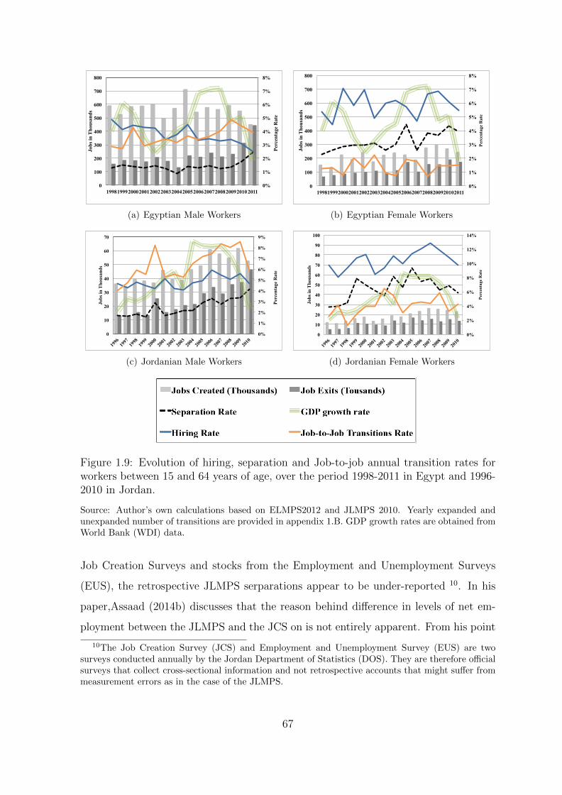
0%

1%

2%

3%

4%

5%

6%

7%

8%

0

100

200

300

400

500

600

700

800

1998 1999 2000 2001 2002 2003 2004 2005 2006 2007 2008 2009 2010 2011

Perc

enta

ge R

ate

Jobs

in T

hous

ands

(a) Egyptian Male Workers

0%

1%

2%

3%

4%

5%

6%

7%

8%

0

100

200

300

400

500

600

700

800

1998 1999 2000 2001 2002 2003 2004 2005 2006 2007 2008 2009 2010 2011

Perc

enta

ge R

ate

Jobs

in T

hous

ands

(b) Egyptian Female Workers

0%

1%

2%

3%

4%

5%

6%

7%

8%

9%

0

10

20

30

40

50

60

70

1996

19

97

1998

19

99

2000

20

01

2002

20

03

2004

20

05

2006

20

07

2008

20

09

2010

Perc

enta

ge R

ate

Jobs

in T

hous

ands

(c) Jordanian Male Workers

0%

2%

4%

6%

8%

10%

12%

14%

0

10

20

30

40

50

60

70

80

90

100

1996

19

97 19

98 19

99 20

00 20

01 20

02 20

03 20

04 20

05 20

06 20

07 20

08 20

09 20

10

Perc

enta

ge R

ate

Jobs

in T

hous

ands

(d) Jordanian Female Workers

Figure 1.9: Evolution of hiring, separation and Job-to-job annual transition rates forworkers between 15 and 64 years of age, over the period 1998-2011 in Egypt and 1996-2010 in Jordan.

Source: Author’s own calculations based on ELMPS2012 and JLMPS 2010. Yearly expanded andunexpanded number of transitions are provided in appendix 1.B. GDP growth rates are obtained fromWorld Bank (WDI) data.

Job Creation Surveys and stocks from the Employment and Unemployment Surveys

(EUS), the retrospective JLMPS serparations appear to be under-reported 10. In his

paper,Assaad (2014b) discusses that the reason behind difference in levels of net em-

ployment between the JLMPS and the JCS on is not entirely apparent. From his point

10The Job Creation Survey (JCS) and Employment and Unemployment Survey (EUS) are twosurveys conducted annually by the Jordan Department of Statistics (DOS). They are therefore officialsurveys that collect cross-sectional information and not retrospective accounts that might suffer frommeasurement errors as in the case of the JLMPS.

67

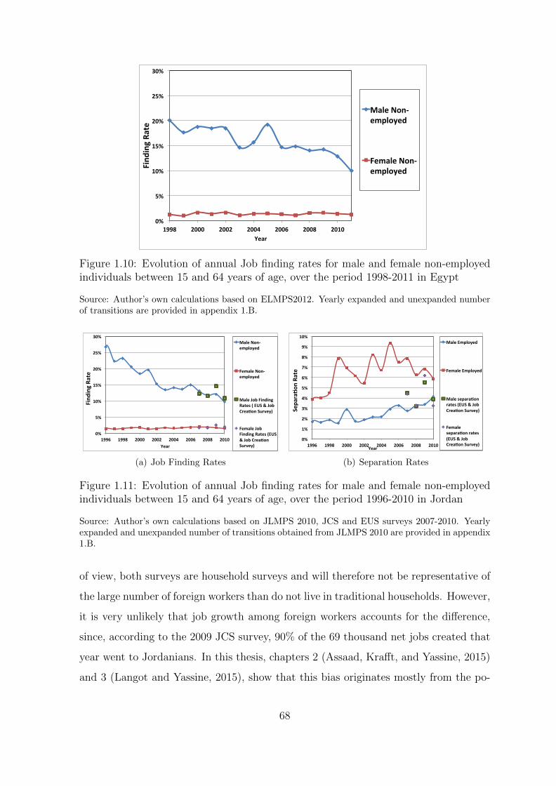
0%

5%

10%

15%

20%

25%

30%

1998 2000 2002 2004 2006 2008 2010

Find

ing Ra

te

Year

Male Non-­‐employed

Female Non-­‐employed

Figure 1.10: Evolution of annual Job finding rates for male and female non-employedindividuals between 15 and 64 years of age, over the period 1998-2011 in Egypt

Source: Author’s own calculations based on ELMPS2012. Yearly expanded and unexpanded numberof transitions are provided in appendix 1.B.

0%

5%

10%

15%

20%

25%

30%

1996 1998 2000 2002 2004 2006 2008 2010

Find

ing Ra

te

Year

Male Non-­‐employed

Female Non-­‐employed

Male Job Finding Rates ( EUS & Job CreaHon Survey)

Female Job Finding Rates (EUS & Job CreaHon Survey)

(a) Job Finding Rates

0%

1%

2%

3%

4%

5%

6%

7%

8%

9%

10%

1996 1998 2000 2002 2004 2006 2008 2010

Sepa

ra2o

n Ra

te

Year

Male Employed

Female Employed

Male separa2on rates (EUS & Job Crea2on Survey)

Female separa2on rates (EUS & Job Crea2on Survey)

(b) Separation Rates

Figure 1.11: Evolution of annual Job finding rates for male and female non-employedindividuals between 15 and 64 years of age, over the period 1996-2010 in Jordan

Source: Author’s own calculations based on JLMPS 2010, JCS and EUS surveys 2007-2010. Yearlyexpanded and unexpanded number of transitions obtained from JLMPS 2010 are provided in appendix1.B.

of view, both surveys are household surveys and will therefore not be representative of

the large number of foreign workers than do not live in traditional households. However,

it is very unlikely that job growth among foreign workers accounts for the difference,

since, according to the 2009 JCS survey, 90% of the 69 thousand net jobs created that

year went to Jordanians. In this thesis, chapters 2 (Assaad, Krafft, and Yassine, 2015)

and 3 (Langot and Yassine, 2015), show that this bias originates mostly from the po-

68

tential measurement errors discussed in the data section, particularly recall and design

bias. Given the availability of data, the comparison between the ELMPS retrospective

data and panel data would therefore be of a valuable further investigation in a separate

research paper to reveal all aspects of such a bias (see chapter 2 (Assaad, Krafft, and

Yassine, 2015)).

It is intuitive and very likely that when reporting their job market histories, indi-

viduals would not recall all (sometimes any of) their unemployment spells, especially

the short ones. Consequently estimates of the separation rates over previous years are

likely to be underestimated. Still, considering the highest value of separation rate in

both time series, Egypt and Jordan, these rates are of an extremely low level. This sug-

gest how rigid the Egyptian and Jordanian labor markets are, where once an individual

finds a job, he/she rarely quits or loses that job before retirement.

It is striking how the Egyptian and Jordanian transition rates, particularly separa-

tion rates, are very low when compared to other countries, even those known for the

rigidity of their labor markets and high employment protection regimes. For instance,

using the French LFS, Hairault, Le Barbanchon, and Sopraseuth (2012) obtained a

corrected monthly French separation probability of 1.2% which is 14.4% yearly.Gomes

(2012) estimated a quarterly average rate of about 3.2% of separations in the UK, which

is 12.8% yearly. In Peru, Herrera and Rosas Shady (2003) estimated the separation

rate of men between 1997 and 1998 of about 12.5% in the urban areas and 4.2% in the

rural areas.

In general, the low transitions rates obtained from the ELMPS and JLMPS retro-

spective panels may be driven by the fact that all spells in the data, whether employ-

ment or non-employment, are truncated from below at six months. The questionnaire

of the survey is designed that way however to avoid all types of casual very short-term

jobs, summer internships..etc. The extent to which such an assumption biases the

transition rates downwards is not thought to be however of a substantial magnitude

given the culture of employment and the nature of labor market institutions in these

countries.

Since recall error is suspected among unemployment spells, these transitions might

be observed in the panel as a job-to-job movement and not necessarily an employment

69

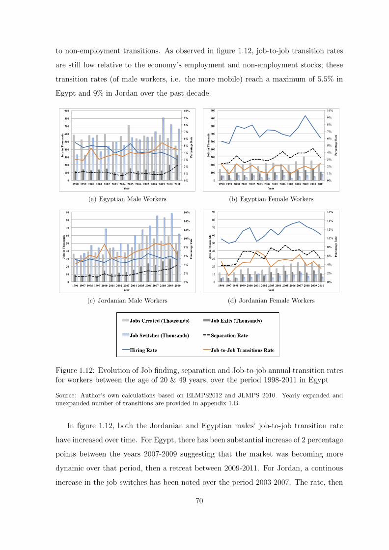
to non-employment transitions. As observed in figure 1.12, job-to-job transition rates

are still low relative to the economy’s employment and non-employment stocks; these

transition rates (of male workers, i.e. the more mobile) reach a maximum of 5.5% in

Egypt and 9% in Jordan over the past decade.

0%

1%

2%

3%

4%

5%

6%

7%

8%

9%

10%

0

100

200

300

400

500

600

700

800

900

1998 1999 2000 2001 2002 2003 2004 2005 2006 2007 2008 2009 2010 2011

Perc

enta

ge R

ate

Jobs

in T

hous

ands

Year

(a) Egyptian Male Workers

0%

1%

2%

3%

4%

5%

6%

7%

8%

9%

10%

0

100

200

300

400

500

600

700

800

900

1998 1999 2000 2001 2002 2003 2004 2005 2006 2007 2008 2009 2010 2011

Perc

enta

ge R

ate

Jobs

in T

hous

ands

Year

(b) Egyptian Female Workers

0%

2%

4%

6%

8%

10%

12%

14%

16%

0

10

20

30

40

50

60

70

80

90

1996 1997 1998 1999 2000 2001 2002 2003 2004 2005 2006 2007 2008 2009 2010

Perc

enta

ge R

ate

Jobs

in T

hous

ands

Year

(c) Jordanian Male Workers

0%

2%

4%

6%

8%

10%

12%

14%

16%

0

10

20

30

40

50

60

70

80

90

1996 1997 1998 1999 2000 2001 2002 2003 2004 2005 2006 2007 2008 2009 2010

Perc

enta

ge R

ate

Jobs

in T

hous

ands

Year

(d) Jordanian Female Workers

Figure 1.12: Evolution of Job finding, separation and Job-to-job annual transition ratesfor workers between the age of 20 & 49 years, over the period 1998-2011 in Egypt

Source: Author’s own calculations based on ELMPS2012 and JLMPS 2010. Yearly expanded andunexpanded number of transitions are provided in appendix 1.B.

In figure 1.12, both the Jordanian and Egyptian males’ job-to-job transition rate

have increased over time. For Egypt, there has been substantial increase of 2 percentage

points between the years 2007-2009 suggesting that the market was becoming more

dynamic over that period, then a retreat between 2009-2011. For Jordan, a continous

increase in the job switches has been noted over the period 2003-2007. The rate, then

70

stabilizes between 2007 and 2009 and finally slowing down between 2009 and 2010.

The increase in the job-to-job transitions in Jordan followed (1)the increase in the

GDP growth rates i.e. the up-turn in the economy and (2)the return of the many

Jordanian emigrants, after the Iraq war in 2003. As the economic growth slows down

in 2007, the increase in the job-to-job transition rates retreats. It is very unlikely that

people change their jobs during the economy’s downturn, i.e. in times of recession

when labor slagness is usually at its maximum. The same scenario applies in Egypt,

especially for the decrease in job switches noted between 2009-2011. This decrease

follows the financial crisis as well as the 25th of January Uprising. The next section

shows that the biggest share of these job-to-job transitions tend to occur within the

informal sector (by workers moving from or to the informal sector), which can simply

be explained by the fact that these are workers, who can not afford being unemployed

and hence move from one informal job to the other, until they are able to find a formal

private or public sector job, if ever.

0.0%

1.0%

2.0%

3.0%

4.0%

5.0%

6.0%

1998

19

99 20

00 20

01 20

02 20

03 20

04 20

05 20

06 20

07 20

08 20

09 20

10 20

11

Perc

enta

ge R

ate

Year

Separation Rate (2006)

Hiring Rate (2006)

Separation Rate (2012)

Hiring Rate (2012)

Figure 1.13: Evolution of job finding and separation (annual) rates for workers betweenthe age of 15 & 49 years, over the period 1998-2011 in Egypt, using ELMPS 2006 andELMPS 2012.

Source: Author’s own calculations based on ELMPS 2006 and ELMPS 2012. Yearly expanded andunexpanded number of transitions obtained from ELMPS 2012 are provided in appendix 1.B. Thepercentage of transitions made by individuals who have also been interviewed in 2006 is also reported.This is particularly important to note how small the sample size can get if one tries to correct mea-surement errors in the data on the micro level (see chapter 5).

Job accession and separation rates are equally important determinants of unem-

ployment fluctuations; it is therefore necessary to analyze the trend of each separately.

71

Figure 1.14 shows the employment inflows, specifically hiring and job finding rates

from inactivity and unemployment, for male workers between 15 and 49 years of age,

in Egypt and Jordan. As explained earlier, when referring to hiring rates, the reference

stock is the stock of employed in year t− 1 while the job finding rates are based on the

unemployed and/or inactive stock in the year t−1. In figure 1.14(a), the unemployment

to employment hiring rate in Egypt is flat over time, while the inactivity to employ-

ment hiring rate has a decreasing trend parallel to the declining working age population

growth. This shows that the general declining trend in the expansion of employment

has been tracking the decline in the growth of the working age population, as the Egyp-

tian youth bulge moves forward over time and gradually gets absorbed in the Egyptian

labor market. In Jordan (figure 1.14(c)), the growth of the working age population has

been constant over time. This has been tracked by a constant trend in the expansion

of employment over time. The composition of hirings has however changed. While

the rate of hirings from inactivity has been declining, it has been compensated by the

increasing hirings from unemployment. As the non-employment to employment finding

rates are plotted in figures 1.14(b) and 1.14(d), it is noted that they decline at a much

faster rate than the hiring and working age population growth rates. The probability

for a non-employed individual to find a job decreases substantially over time especially

among the new labor entrants, as shown by the decreasing inactivity to employment

finding rates. A sudden decline in the inactivity to employment finding rate is observed

in Egypt between 2009-2011, showing possibly that the situation gets even worse with

the financial crisis and the January 2011 Uprising after which the rate dropped by

about 10 percentage points from 25% to 15%. This drop suggests that new entrants

are taking longer to find jobs after the January 2011 Uprising. Consequently, in 2011,

an Egyptian inactive person (most probably a new entrant) has an annual probability

of 15% to find a job, while an unemployed person has an annual probability of 30%.

Again, the fact that this sudden decline is the image of the sharp increase observed

in the separation rates and that it is kind of observed in similar patterns in both the

ELMPS and the JLMPS, suggests that this might be partially artificial and requires

further investigation. In Jordan, in 2009, the gap between the job finding probability

between an unemployed and inactive is even wider than in Egypt, with a job finding

72

rate of 40% for the unemployed and 7% for the inactives. These estimates therefore

suggest that an Egyptian unemployed can stay up to 3 years until he finds his next

job, while in Jordan, it would take him about 2.5 years. Comparing these values to

other countries the Egyptian and Jordanian labor markets have a problem in the job

finding process. Even among existing jobs (whether old or newly created), there are

obstacles on both the labor demand and supply sides to becoming matched. According

to Hairault, Le Barbanchon, and Sopraseuth (2012), the average monthly French job

finding probability amounts to 7.5%(90% yearly).

0%

1%

2%

3%

4%

5%

1998 2000 2002 2004 2006 2008 2010

Flow

s Rate

Year

(a) Hiring Rates and Working Populationgrowth rate in Egypt

0%

5%

10%

15%

20%

25%

30%

35%

40%

1998 2000 2002 2004 2006 2008 2010

Flow

s Rate

Year

(b) Job Finding Rates and Working Populationgrowth rate in Egypt

0%

1%

2%

3%

4%

5%

6%

1996 1998 2000 2002 2004 2006 2008

Fows R

ate

Year

(c) Hiring Rates and Working Populationgrowth rate in Jordan

0%

5%

10%

15%

20%

25%

30%

35%

40%

45%

1996 1998 2000 2002 2004 2006 2008

Fows R

ate

Year

(d) Job Finding Rates and Working Populationgrowth rate in Jordan

Figure 1.14: Employment Inflows Annual Hiring and Job Finding Rates, Male Workersbetween 15 & 49 years of age, over the period 2000-2011.

Source: Author’s own calculations based on ELMPS2012 and JLMPS 2010. Yearly expanded andunexpanded number of transitions are provided in appendix 1.B.

73

Turning now to the employment outflows in figures 1.15 and 1.16, the observation

period has been dominated by two main trends for both employment to unemploy-

ment and employment to inactivity transition rates in Egypt and for employment to

unemployment in Jordan. In Egypt, between 2000-2009, the employment to unem-

ployment separation rate follows a slightly increasing trend, while the employment to

inactivity rate declines from about 0.6% to 0.3%. This further analysis of employment

outflows has revealed that the separation rates, both employment to unemployment

and employment to inactivity, experienced a huge increase after 2009 of almost 0.8 (to

unemployment) and 0.5 percentage points (to inactivity). In Jordan, the employment

to unemployment separation rate reamined constant over the period 1996-2003, then

increased substantially after 2003 by about 1.7 percent. The employment to inactiv-

ity separations, on the other side, have been continously slightly increasing over time.

These trends, as have been mentioned previously, are questionable and are to be studied

in the following chapters.

0.0%

0.2%

0.4%

0.6%

0.8%

1.0%

1.2%

1998 1999 2000 2001 2002 2003 2004 2005 2006 2007 2008 2009 2010 2011

Flow

s Rate

Year

Figure 1.15: Employment Outflows Annual Separation Rates, Male Workers between15 and 49 years of age, Egypt 1998-2011.

Source: Author’s own calculations based on ELMPS2012. Yearly expanded and unexpanded numberof transitions are provided in appendix 1.B.

It is important to note however that the separation rates remain at relatively low

levels with respect to the persistent high non-employment stock in both economies.

Moreover, the detection of the inflection point in the separations in Egypt could be

partly explained by a reaction to the slowdown of economic growth following the fi-

74

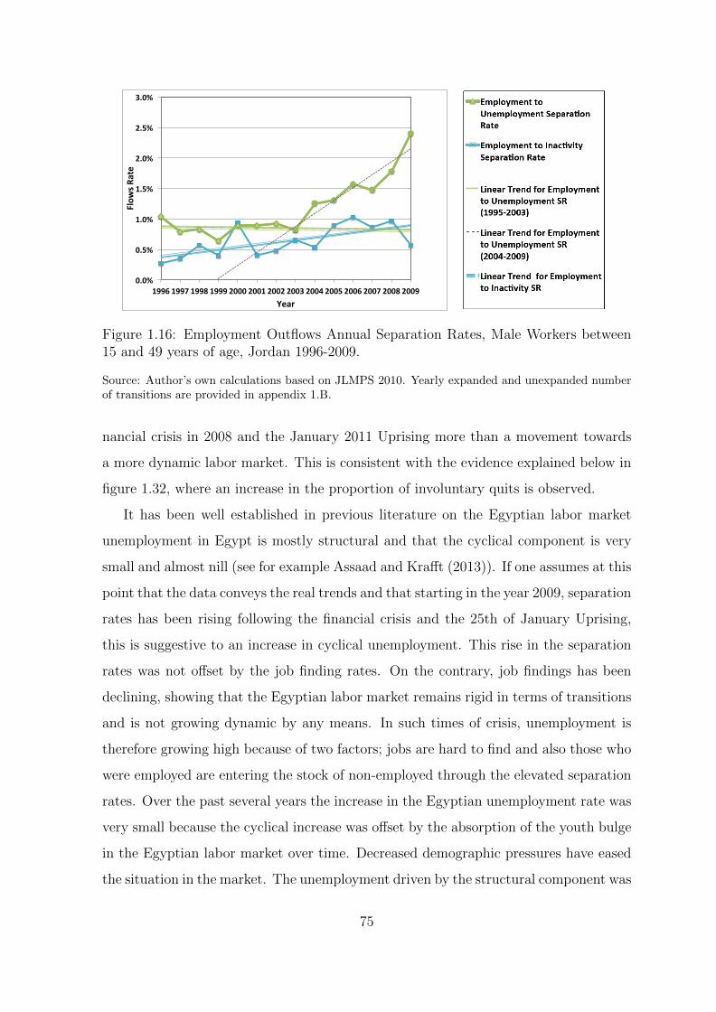
0.0%

0.5%

1.0%

1.5%

2.0%

2.5%

3.0%

1996 1997 1998 1999 2000 2001 2002 2003 2004 2005 2006 2007 2008 2009

Flow

s Rate

Year

Figure 1.16: Employment Outflows Annual Separation Rates, Male Workers between15 and 49 years of age, Jordan 1996-2009.

Source: Author’s own calculations based on JLMPS 2010. Yearly expanded and unexpanded numberof transitions are provided in appendix 1.B.

nancial crisis in 2008 and the January 2011 Uprising more than a movement towards

a more dynamic labor market. This is consistent with the evidence explained below in

figure 1.32, where an increase in the proportion of involuntary quits is observed.

It has been well established in previous literature on the Egyptian labor market

unemployment in Egypt is mostly structural and that the cyclical component is very

small and almost nill (see for example Assaad and Krafft (2013)). If one assumes at this

point that the data conveys the real trends and that starting in the year 2009, separation

rates has been rising following the financial crisis and the 25th of January Uprising,

this is suggestive to an increase in cyclical unemployment. This rise in the separation

rates was not offset by the job finding rates. On the contrary, job findings has been

declining, showing that the Egyptian labor market remains rigid in terms of transitions

and is not growing dynamic by any means. In such times of crisis, unemployment is

therefore growing high because of two factors; jobs are hard to find and also those who

were employed are entering the stock of non-employed through the elevated separation

rates. Over the past several years the increase in the Egyptian unemployment rate was

very small because the cyclical increase was offset by the absorption of the youth bulge

in the Egyptian labor market over time. Decreased demographic pressures have eased

the situation in the market. The unemployment driven by the structural component was

75

actually decreasing (Assaad and Krafft, 2013). This should be a source of worry, since in

the near future, the echo of the youth bulge in Egypt will enter the labor market causing

extra pressure and a rising structural unemployment trend worsening the situation and

causing the rate of unemployment to increase substantially. Consequently and in that

case, one would expect, over the long run, a substantial increase in the prevailing

Egyptian unemployment rate if job finding probability of the non-employed continues

to fall, separation rate continues to rise along with the increasing demographic pressures

resulting from the echo of the youth bulge.

1.5 Characterizing Labor Market Flows

In this section, the aim is to characterize the job flows observed above, specifically

job accession, separation and mobility. With a focus on the observed transitions out

of employment after 2009 for Egypt and after 2003 for Jordan, the analysis illustrates

the individuals’ and firms’ characteristics that tend to affect the likelihood of staying

in, leaving/quitting or switching jobs. It is important to note at this point that when

analyzing a job quit/leave or a job-to-job switch, the characteristics of the job before

the change occurs (the characteristics of the origin job status) are explored. When

discussing a job accession, the characteristics of the new job created after transition

(the destination job status) are analyzed.

1.5.1 Characteristics of the Egyptian and Jordanian Job Flows

Figures 1.17-1.19 show the evolution of the mean age of male workers in each type

of transition over the observation period for both Egypt and Jordan. In both countries,

entrants to the labor market from inactivity are younger than those entering from the

unemployment stocks. This verifies the fact that these represent the new labor market

entrants, who are accessing jobs for the first time in their labor market history. Indi-

viduals accessing jobs in Jordan from unemployment are however slightly older than

their Egyptian peers. In Jordan, workers moving out of employment to an unemploy-

ment spell are on average younger than those transiting from employment to inactivity.

These job quitters/losers are older than the sample’s average and are also much older

76

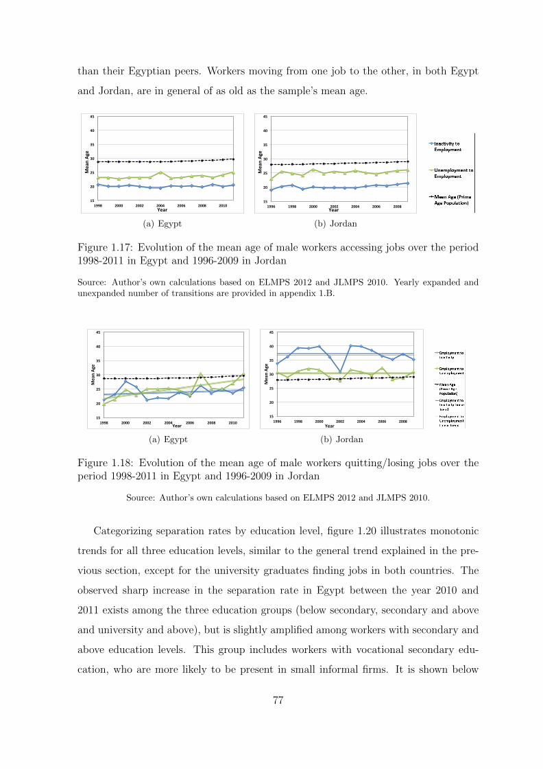
than their Egyptian peers. Workers moving from one job to the other, in both Egypt

and Jordan, are in general of as old as the sample’s mean age.

15

20

25

30

35

40

45

1998 2000 2002 2004 2006 2008 2010

Mean Ag

e

Year

(a) Egypt

15

20

25

30

35

40

45

1996 1998 2000 2002 2004 2006 2008

Mean Ag

e

Year

(b) Jordan

Figure 1.17: Evolution of the mean age of male workers accessing jobs over the period1998-2011 in Egypt and 1996-2009 in Jordan

Source: Author’s own calculations based on ELMPS 2012 and JLMPS 2010. Yearly expanded andunexpanded number of transitions are provided in appendix 1.B.

15

20

25

30

35

40

45

1998 2000 2002 2004 2006 2008 2010

Mean Ag

e

Year

(a) Egypt

15

20

25

30

35

40

45

1996 1998 2000 2002 2004 2006 2008

Mean Ag

e

Year

(b) Jordan

Figure 1.18: Evolution of the mean age of male workers quitting/losing jobs over theperiod 1998-2011 in Egypt and 1996-2009 in Jordan

Source: Author’s own calculations based on ELMPS 2012 and JLMPS 2010.

Categorizing separation rates by education level, figure 1.20 illustrates monotonic

trends for all three education levels, similar to the general trend explained in the pre-

vious section, except for the university graduates finding jobs in both countries. The

observed sharp increase in the separation rate in Egypt between the year 2010 and

2011 exists among the three education groups (below secondary, secondary and above

and university and above), but is slightly amplified among workers with secondary and

above education levels. This group includes workers with vocational secondary edu-

cation, who are more likely to be present in small informal firms. It is shown below

77

15

20

25

30

35

40

45

1998 2000 2002 2004 2006 2008 2010

Mean Ag

e

Year

(a) Egypt

15

20

25

30

35

40

45

1996 1998 2000 2002 2004 2006 2008

Mean Ag

e

Year

(b) Jordan

Figure 1.19: Evolution of the mean age of male workers switching from job to the otherover the period 1998-2011 in Egypt and 1996-2009 in Jordan

Source: Author’s own calculations based on ELMPS 2012 and JLMPS 2010.

that workers within informal employment experienced a large increase in separation

rates of about 1.5 percentage points between the years 2010 and 2011. In Jordan, the

continously increasing trend is observed for the below secondary and secondary groups.

For the university graduates, the increasing trend is observed up to 2006, but after-

wards the curve gets fuzzy possibly due to the small number of observations (the point

in 2006 is most probably an outlier). Generally however and in both countries, the

most educated group of workers are the least probable to quit or lose their jobs. Their

separation rates are the lowest (sometimes almost nil). For the labor market entrants,

education seems to play an important role over the observation period. Observing the

trends for the job finding probability of a non-employed person, it is interesting that

over time and in both countries, it is first observed up to 3 years before the year of the

survey, that it’s the most difficult for a university graduate to find a job. This ranking

is however reversed in the last three years, which again confirms a potential bias in

these trends especially in the very old years of the retrospective panels. It is interesting

to note however, that the university and above educated group appear to be the least

affected by the drop in the job finding rates observed after the financial crisis and the

January 2011 Uprising, in the case of Egypt. Yet again, these trends seem to be very

artificial with an abrupt increase in the finding rates 3 years prior to the survey in both

countries.

As for the transitions from one job to the other, the least educated group in Egypt

seems to be the most stable. These workers are more likely to be poor. They can not

78

afford to be unemployed and since their job finding probability from unemployment is

low, they will not search (on-the-job search) unless they are forced to leave their job.

In Jordan, no much difference is observed between the different education groups.

To examine dynamics by the type and sector of employment, figures 1.21-1.28 show

that generally non-wage workers experience very little changes over time of relatively

lower transition rates (accession, separation and mobility). Interestingly, for the job-to-

job transitions in both countries, some points are as high as the wage workers’ though.

All the observed turnover however seems to occur among the wage workers whether

discussing job accession, separation or mobility. Moreover as public and private wage

employment are distinguished, one notes that job-to-job transitions for the public sector

are generally lower in both Egypt and Jordan, while separations are extremely low for

the government employees in Egypt. Wage workers who are losing their jobs are mainly

workers in the informal sector while those moving from one job to the other are those

employed in both informal and formal private sector (with the informal sector having

slightly higher rates). In Jordan, the differences between the formal and informal sectors

in terms of both their separations and job-to-job transitions are much less emphasized

than in Egypt. It’s true that this might be due to the fact that the Jordanian labor

market has been liberalized earlier than the Egyptian, but could also be a signal to how

much more segmented it might be, especially that the difference between the different

sectors’ job finding rates is minimal while in Egypt, the sector that a job seeker is

targeting matters a lot. In Egypt, workers tend to take the informal sector as an

intermediary waiting for a formal job either in the private or the public sector (which

have much lower job finding rates) depending on their preference. In Jordan, this does

not seem to be the case, where the labor market appears to be segmented and its

segments are functioning in parallel. Workers are finding jobs in the three sectors at

the same rate, probably because workers are getting hired in the sector that is most

suitable for them and relevant for their case. It is also important to note that private

wage workers have the highest job-to-job transition rates especially in the most recent

years, which are most likely the most reliable years. The sharp increase in separations

in Egypt was exclusively limited to the private sector wage workers. According to these

raw data flows, both formal and informal private wage workers experienced an increase

79

0.0%

1.0%

2.0%

3.0%

4.0%

5.0%

1998 1999 2000 2001 2002 2003 2004 2005 2006 2007 2008 2009 2010 2011

Percen

tage Rate

Year

(a) Employment to Non-employment (Egypt)

0.0%

0.5%

1.0%

1.5%

2.0%

2.5%

3.0%

3.5%

4.0%

4.5%

5.0%

1996 1997 1998 1999 2000 2001 2002 2003 2004 2005 2006 2007 2008 2009

Percen

tage Rate

Year

(b) Employment to Non-employment (Jordan)

0%

5%

10%

15%

20%

25%

30%

35%

40%

45%

50%

1998 1999 2000 2001 2002 2003 2004 2005 2006 2007 2008 2009 2010 2011

Percen

tage Rate

Year

(c) Non-Employment to Employment (Egypt)

0%

5%

10%

15%

20%

25%

30%

35%

40%

45%

50%

1996 1997 1998 1999 2000 2001 2002 2003 2004 2005 2006 2007 2008 2009

Percen

tage Rate

Year

(d) Non-Employment to Employment (Jordan)

0%

2%

4%

6%

8%

10%

12%

1998 1999 2000 2001 2002 2003 2004 2005 2006 2007 2008 2009 2010 2011

Percen

tage Rate

Year

(e) Job-to-Job (Egypt)

0%

2%

4%

6%

8%

10%

12%

1996 1997 1998 1999 2000 2001 2002 2003 2004 2005 2006 2007 2008 2009

Percen

tage Rate

Year

(f) Job-to-Job (Jordan)

Figure 1.20: Evolution of transition rates for male workers, between 15 and 49 years ofage, by education level in Egypt and Jordan

Source: Author’s own calculations based on ELMPS 2012 and JLMPS 2010.

80

0%

2%

4%

6%

8%

10%

12%

14%

16%

18%

20%

1998 1999 2000 2001 2002 2003 2004 2005 2006 2007 2008 2009 2010 2011

Percen

tage Rate

Year

Wage Workers Non-­‐Wage Workers

(a)

0% 2% 4% 6% 8% 10% 12% 14% 16% 18% 20%

1998 1999 2000 2001 2002 2003 2004 2005 2006 2007 2008 2009 2010 2011

Percen

tage Rate

Year

Public WW Formal PRWW Informal PRWW

(b)

Figure 1.21: Evolution of job finding rates for male workers, between 15 and 49 yearsof age, by type and sector of employment in Egypt.

Source: Author’s own calculations based on ELMPS 2012.

0%

1%

2%

3%

4%

5%

6%

7%

1998 1999 2000 2001 2002 2003 2004 2005 2006 2007 2008 2009 2010 2011

Percen

tage Rate

Year Wage Workers Non-­‐Wage Workers

(a)

0%

1%

2%

3%

4%

5%

6%

7%

8%

9%

1998 1999 2000 2001 2002 2003 2004 2005 2006 2007 2008 2009 2010 2011

Percen

tage Rate

Year

Public WW Formal PRWW Informal PRWW

(b)

Figure 1.22: Evolution of hiring rates for male workers, between 15 and 49 years ofage, by type and sector of employment, in Egypt.

Source: Author’s own calculations based on ELMPS 2012.

in separations, of about two percentage points each. Following the reasoning that part

of this increase is tracking the downturn in the economy, obviously both formal and

informal employers resorted to large-scale layoffs during the crises of 2009 and 2011, in

addition to hours or wages reductions.

Figure 1.29 highlights the distribution of wage workers who quit or lose their jobs

over time. The pattern in general confirms that the majority of workers losing or quit-

ting their jobs are originally wage workers in the informal sector. The most noticeable

though is the slightly increasing trend in Egypt in the share of formal wage employment

over time. This share has however been stable or slightly declining in Jordan.

As observed based on the job-to-job transitions in figure 1.30, the increasing trend

81

0.0%

0.5%

1.0%

1.5%

2.0%

2.5%

3.0%

3.5%

1998 1999 2000 2001 2002 2003 2004 2005 2006 2007 2008 2009 2010 2011

Percen

tage Rate

Year Wage Workers Non-­‐Wage Workers

(a)

0.0%

0.5%

1.0%

1.5%

2.0%

2.5%

3.0%

3.5%

1998 1999 2000 2001 2002 2003 2004 2005 2006 2007 2008 2009 2010 2011

Percen

tage Rate

Year Public WW Formal PRWW Informal PRWW

(b)

Figure 1.23: Evolution of separation rates for male workers, between 15 and 49 yearsof age, by type and sector of employment, in Egypt.

Source: Author’s own calculations based on ELMPS 2012.

0%

1%

2%

3%

4%

5%

6%

7%

1998 1999 2000 2001 2002 2003 2004 2005 2006 2007 2008 2009 2010 2011

Percen

tage Rate

Year

Wage Workers Non-­‐Wage Workers

(a)

0%

1%

2%

3%

4%

5%

6%

7%

8%

1998 1999 2000 2001 2002 2003 2004 2005 2006 2007 2008 2009 2010 2011

Percen

tage Rate

Year

Public Formal WW Informal WW

(b)

Figure 1.24: Evolution of job-to-job transition rates for male workers, between 15 and49 years of age, by type and sector of employment, in Egypt.

Source: Author’s own calculations based on ELMPS 2012.

0%

5%

10%

15%

20%

25%

30%

1995 1996 1997 1998 1999 2000 2001 2002 2003 2004 2005 2006 2007 2008

Percen

tage Rate

Year

Wage Workers Non-­‐Wage Workers

(a)

0%

2%

4%

6%

8%

10%

12%

14%

16%

18%

20%

1995 1996 1997 1998 1999 2000 2001 2002 2003 2004 2005 2006 2007 2008

Percen

tage Rate

Year

Public WW Formal PRWW Informal PRWW

(b)

Figure 1.25: Evolution of job finding rates for male workers, between 15 and 49 yearsof age, by type and sector of employment, in Jordan.

Source: Author’s own calculations based on JLMPS 2010.

82

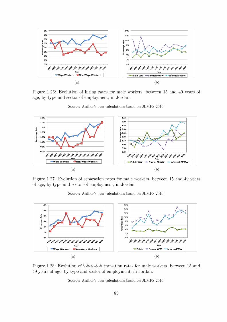
0%

1%

2%

3%

4%

5%

6%

7%

8%

1995 1996 1997 1998 1999 2000 2001 2002 2003 2004 2005 2006 2007 2008

Percen

tage Rate

Year Wage Workers Non-­‐Wage Workers

(a)

0%

2%

4%

6%

8%

10%

12%

14%

1995 1996 1997 1998 1999 2000 2001 2002 2003 2004 2005 2006 2007 2008

Percen

tage Rate

Year

Public WW Formal PRWW Informal PRWW

(b)

Figure 1.26: Evolution of hiring rates for male workers, between 15 and 49 years ofage, by type and sector of employment, in Jordan.

Source: Author’s own calculations based on JLMPS 2010.

0.0%

0.5%

1.0%

1.5%

2.0%

2.5%

3.0%

3.5%

1995 1996 1997 1998 1999 2000 2001 2002 2003 2004 2005 2006 2007 2008

Percen

tage Rate

Year Wage Workers Non-­‐Wage Workers

(a)

0.0%

0.5%

1.0%

1.5%

2.0%

2.5%

3.0%

3.5%

4.0%

4.5%

1995 1996 1997 1998 1999 2000 2001 2002 2003 2004 2005 2006 2007 2008

Percen

tage Rate

Year Public WW Formal PRWW Informal PRWW

(b)

Figure 1.27: Evolution of separation rates for male workers, between 15 and 49 yearsof age, by type and sector of employment, in Jordan.

Source: Author’s own calculations based on JLMPS 2010.

0%

2%

4%

6%

8%

10%

12%

1995 1996 1997 1998 1999 2000 2001 2002 2003 2004 2005 2006 2007 2008

Percen

tage Rate

Year Wage Workers Non-­‐Wage Workers

(a)

0%

2%

4%

6%

8%

10%

12%

14%

16%

1995 1996 1997 1998 1999 2000 2001 2002 2003 2004 2005 2006 2007 2008

Percen

tage Rate

Year

Public Formal WW Informal WW

(b)

Figure 1.28: Evolution of job-to-job transition rates for male workers, between 15 and49 years of age, by type and sector of employment, in Jordan.

Source: Author’s own calculations based on JLMPS 2010.

83

0%

10%

20%

30%

40%

50%

60%

70%

1998 2000 2002 2004 2006 2008 2010

Percen

t

Year

(a) Egypt

0%

10%

20%

30%

40%

50%

60%

70%

80%

90%

1996 1998 2000 2002 2004 2006 2008 2010

Percen

t

Year

(b) Jordan

Figure 1.29: Distribution of private wage workers who quit/lose their jobs over time byformality and in/out of establishment.

Source: Author’s own calculations based on ELMPS 2012 and JLMPS 2010.

0%

10%

20%

30%

40%

50%

1998 2000 2002 2004 2006 2008 2010

Percen

t

Year

(a) Egypt

0%

10%

20%

30%

40%

50%

1996 1998 2000 2002 2004 2006 2008 2010

Percen

t

Year

(b) Jordan

Figure 1.30: Distribution of private wage workers who move from one job to another(job-to-job transition) over time by formality and in/out of establishment of the sourcejob.

Source: Author’s own calculations based on ELMPS 2012 and JLMPS 2010.

of transitions over time is driven primarily by informal workers. The distribution of

workers who switch to new jobs over the observation period by formality and in/out

of establishment (for their job destination) in figure 1.31 shows that on average only

about 40% of wage workers transiting from previous jobs (whether formal or informal)

move to formal jobs afterwards. The trend of this share has either been stable over time

(as in Egypt) or declining (as in Jordan). The remaining 60% are distributed between

workers who find jobs the informal wage work sector inside and outside establishments.

In Jordan, 60% of the job-to-job transitions originated from the informal sector. The

share of workers who manage to move to a formal job destination declined from 45% to

40% over the period 1996-2010. This is another source of worry for both the Egyptian

84

0%

10%

20%

30%

40%

50%

1998 2000 2002 2004 2006 2008 2010

Percen

t

Year

(a) Egypt

0%

10%

20%

30%

40%

50%

1996 1998 2000 2002 2004 2006 2008 2010

Percen

t

Year

(b) Jordan

Figure 1.31: Distribution of private wage workers who who move from one job to an-other (job-to-job transition) by formality and in/out of establishment of the destinationjob.

Source: Author’s own calculations based on ELMPS 2012 and JLMPS 2010.

and Jordanian labor markets, which are not only characterized by relatively low job-to-

job transition rates but if these transitions do take place, they occur among workers who

have a low “reservation” package or low expectations ( reservation offer including the

wage level, work conditions, job quality, formality, productivity, skills level required...).

These workers do get affected by the downturns of the economy and the slowdown in

economic growth but since they cannot afford to stay unemployed, they would rather

move to and accept informal jobs. This for instance might explain the small increase

noted in the unemployment rates in Egypt in recent years even though one would have

expected a large increase in these rates after the financial crisis and the January 2011

Uprising.

Having discussed the age, education and sector of employment of wage workers

transiting from one state or job to another, it is crucial at this point to explore the

reason of transition for these workers. Unfortunately, this question was not available in

the JLMPS (see section 1.3.1). The analysis is therefore only done for Egypt. In figure

1.32, the evolution of the share of voluntary and involuntary movers is plotted. An

involuntary leave or job switch is one which was out of the worker’s hands and where

he was forced to transit to another state or job.

In general, job quits and job-to-job transitions have been mainly driven over the

past decade by the worker’s will and desire. In the year 2005, 90% of male workers who

moved out of employment were quitting their jobs voluntarily, and 85% were willingly

85

0%

10%

20%

30%

40%

50%

60%

70%

80%

90%

100%

1998 2000 2002 2004 2006 2008 2010

Percen

t

Year

Involuntary Separa=ons

Voluntary Separa=ons

Linear Trend of Involuntary Separa=ons

Linear Trend of Voluntary Separa=ons

(a) Employment to non-employment transi-tions

0%

10%

20%

30%

40%

50%

60%

70%

80%

90%

100%

1998 2000 2002 2004 2006 2008 2010

Percen

t

Year

Involuntary Job-­‐to-­‐Job Transi2ons

Voluntary Job-­‐to-­‐Job Transi2ons

Linear Trend of involuntary job-­‐to-­‐job transi2ons

Linear Trend of voluntary job-­‐to-­‐job transi2ons

(b) Job-to-job transitions

Figure 1.32: Distribution of employment to non-employment (separations) and job-to-job transitions over the period 1998-2012 in Egypt, by reason of change.

Source: Author’s own calculations based on ELMPS 2012.

switching to another job. Unsurprisingly, the share of involuntary leaves increased over

the period 2009-2012. These were mainly workers who reported that their contracts

were ended and not renewed by the employer. This might provide additional evidence

that the increase in separations observed in the previous sections was a reaction to the

economic downturn, and not purely an artificial increase due to recall and misreporting

problems. Trends in involuntary job switches have remained stable with a slight increase

between the years 2010 and 2011. This increase was mainly due to workers who searched

for other jobs because they were terminated by their employers or were working in a

project that got suspended.

1.6 Conclusion

The objective of this paper is to set out a number of stylized facts about the Egyp-

tian and Jordanian labor market flows over the past decade using the ELMPS and

JLMPS datasets. Although it is descriptive by nature, the main contribution of this

paper is to provide a summary of a wide range of information about Egyptian and

Jordanian labor market dynamics from several different angles. The paper provides

a survey of the different labor market institutions in Egypt and Jordan. These are

markets with generally low levels of employment, higher youth unemployment rate,

oversized public sectors and large informal sectors. This paper also provides a descrip-

86

tion of the questionnaires structures of the datasets to be used in this thesis. It also

details the steps adopted to extract longitudinal retrospective datasets. This is crucial

for developing countries such as Egypt and Jordan where limited budget constraints do

not allow regular panel data collection needed for analysis of labor market dynamics.

The labor market dynamics stylized facts deduced in this paper are the first of

this kind and may prove useful to researchers and policy-makers working on various

aspects of the Egyptian and Jordanian labor markets. Knowledge of those facts is

crucial to be able to monitor business cycles, detect inflection points and assess labor

market tightness (how labor demand and supply are balanced within the economy).

It is important to ensure a healthy dynamic labor market where productive jobs are

being created, existing jobs are getting more productive and less productive jobs are

being destroyed. This does not seem to be happening at all in the Egyptian and

Jordanian labor markets where most of the turnover is occurring in small informal

sector jobs, job-to-job transitions are extremely low and when they occur it is because

people are moving within or to the informal sector. One has to note though that the

Jordanian labor market, given the history and evolution of its regulatory institutional

framework, it is more flexible and mobile than the Egyptian labor market. Yet, there is

some evidence that suggests that the Jordanian labor market is much more segmented

than the Egyptian; the informal sector serving mostly as an intermediary in Egypt,

while in Jordan it appears to be a segment in the market that functions on its own

attracting specific workers. The informality aspect of both markets surely requires more

investigation and further research. In Egypt, the formal public and private sectors

suffer from an extremely rigid environment where workers, once they access jobs in

these sectors, would hardly ever leave or move to other jobs. In general, separation

rates in Egypt are extremely low. The trends of flows in this paper show however that

there have been better responses to the economic slowdown from the private formal

sector than before, especially after January 2011 Uprising. Overall, the sluggishness

of the Egyptian and Jordanian labor markets is surely hindering to a large extent the

productivity levels and growth within the economy.

The main findings of this paper confirm the fact that unemployment in Egypt tends

to be dominated by structural rather than cyclical. The trends obtained from the raw

87

data might suggest an increasing role of cyclical unemployment in the Egyptian labor

market starting in 2009, as a reaction to the financial crisis as well as the January

2011 Uprising. In Jordan, the unemployment components, namely job findings and

separations seem to be changing trends after 2003, i.e. after the return of Jordanians

after the Iraq war and also after the slowdown of the GDP growth rates in 2007.

The Egyptian and Jordanian labor markets are two arab MENA countries that suffer

from low job accession, separation and mobility rates relative to stocks of employment

and unemployment. The paper notes a declining trend in the Egyptian hiring rates,

mirroring the falling trend in the working age population growth rate, showing that

the youth bulge was successfully absorbed in the Egyptian Labor Market over the past

decade. It also shows a constant trend of employment expansion in Jordan tracking the

stagnant population growth rate. However, trends show that it became more difficult

for a non-employed individual to find jobs. Rates of workers quitting their jobs or

getting laid off remain at a low level even after an apparent increase in the most recent

years of the retrospective panels i.e. the years right before the year of the survey.

One has to be cautious when analysing such results given the potential biases and

measurement errors in the datasets used that might result in artificial variations in levels

or trends. Indeed, the results suggest that separation rates reach their highest levels in

2011 in Egypt and 2010 in Jordan, however this is only 2% of the total employment in

Egypt and 4% in Jordan. The analysis shows that the share of involuntary job loss has

increased over the period 2009-2011 in Egypt. This supports that these trends reflect

the response of the Egyptian labor market to the financial crisis and the January 2011

Uprising rather than a more dynamic labor market. However, one cannot confirm this

conclusion given potential recall errors and questionnaire design bias. The following

chapters investigate these errors and offer possible solutions and corrections to be able

to use the data to analyze the dynamics of the labor market in question.

The analysis also shows evidence of increasing trends of job-to-job transition rates

in Egypt, especially among informal workers. In general, the formal sector remains

rigid although evidence of better responses to the economic slowdown from the private

formal sector, than from the public sector, has been documented. The overall picture

suggests that the Egyptian and Jordanian labor markets should be a source of worry.

88

Future unemployment rates, particularly in Egypt, are expected to be substantially

higher due to the the increasing separations and declining job finding, as well as higher

demographic pressures resulting from the echo of the youth bulge.

89

References

Amin, M., R. Assaad, N. al Baharna, K. Dervis, R. M. Desai, N. S.

Dhillon, and A. Galal (2012): After the spring: Economic transitions in the

Arab world. Oxford University Press.

Assaad, R. (2014a): “Making sense of Arab labor markets: the enduring legacy of

dualism,” IZA Journal of Labor & Development, 3(1), 1–25.

(2014b): “The structure and evolution of employment in Jordan,” The Jorda-

nian Labour Market in the New Millennium, pp. 1–38.

Assaad, R., and C. Krafft (2013): “The Egypt labor market panel survey: intro-

ducing the 2012 round,” IZA Journal of Labor & Development, 2(1), 8.

Assaad, R., C. Krafft, and C. Yassine (2015): “Comparing Retrospective and

Panel Data Collection Methods to Assess Labor Market Dynamics,” Discussion pa-

per, Economic Research Forum, Cairo.

Blanchard, O. J., P. Diamond, R. E. Hall, and K. Murphy (1990): “The

cyclical behavior of the gross flows of US workers,” Brookings Papers on Economic

Activity, pp. 85–155.

Bleakley, H., A. E. Ferris, and J. C. Fuhrer (1999): “New data on worker

flows during business cycles,” New England Economic Review, pp. 49–76.

Davis, S. J., J. C. Haltiwanger, and S. Schuh (1996): “Job Creation and De-

struction,” Massachusetts Institute of Technology, Cambridge, MA.

Desai, R. M., A. Olofsgard, and T. M. Yousef (2009): “The logic of authori-

tarian bargains,” Economics & Politics, 21(1), 93–125.

90

Fujita, S., and G. Ramey (2009): “The cyclicality of separation and job finding

rates,” International Economic Review, 50(2), 415–430.

Gatti, R., D. F. Angel-Urdinola, J. Silva, and A. Bodor (2014): Striving

for Better Jobs: The Challenge of Informality in the Middle East and North Africa.

World Bank Publications.

Gatti, R., M. Morgandi, R. Grun, S. Brodmann, D. Angel-Urdinola, and

J. M. Moreno (2013): Jobs for shared prosperity: time for action in the Middle

East and North Africa. World Bank Publications.

Gomes, P. (2012): “Labour market flows: facts from the United Kingdom,” Labour

Economics, 19(2), 165–175.

Hairault, J.-O., T. Le Barbanchon, and T. Sopraseuth (2012): “The cyclical-

ity of the separation and job finding rates in France,”Discussion paper, Forschungsin-

stitut zur Zukunft der Arbeit.

Herrera, J., and G. D. Rosas Shady (2003): “Labor market transitions in Peru,”

Discussion paper, DIAL.

Langot, F., and C. Yassine (2015): “Reforming employment protection in Egypt:

An evaluation based on transition models with measurement errors,” Discussion pa-

per, Economic Research Forum, Cairo.

Loayza, N., and T. Wada (2010): “Informal labor in the Middle East and North

Africa: Basic measures and determinants,” Washington, DC: World Bank.

Schneider, F., A. Buehn, and C. E. Montenegro (2010): “New Estimates for

the Shadow Economies all over the World,” International Economic Journal, 24(4),

443–461.

Shimer, R. (2012): “Reassessing the ins and outs of unemployment,” Review of Eco-

nomic Dynamics, 15(2), 127–148.

91

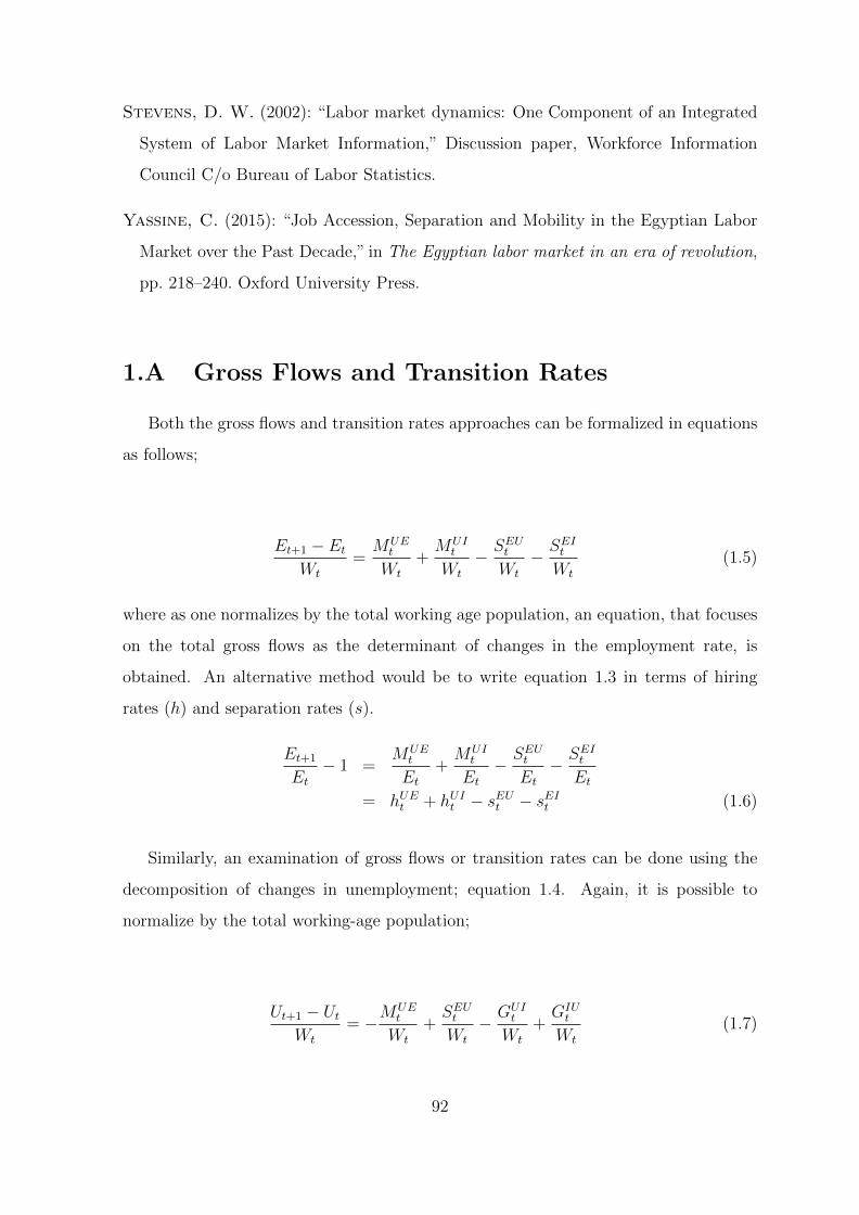
Stevens, D. W. (2002): “Labor market dynamics: One Component of an Integrated

System of Labor Market Information,” Discussion paper, Workforce Information

Council C/o Bureau of Labor Statistics.

Yassine, C. (2015): “Job Accession, Separation and Mobility in the Egyptian Labor

Market over the Past Decade,” in The Egyptian labor market in an era of revolution,

pp. 218–240. Oxford University Press.

1.A Gross Flows and Transition Rates

Both the gross flows and transition rates approaches can be formalized in equations

as follows;

Et+1 − EtWt

=MUE

t

Wt

+MUI

t

Wt

− SEUtWt

− SEItWt

(1.5)

where as one normalizes by the total working age population, an equation, that focuses

on the total gross flows as the determinant of changes in the employment rate, is

obtained. An alternative method would be to write equation 1.3 in terms of hiring

rates (h) and separation rates (s).

Et+1

Et− 1 =

MUEt

Et+MUI

t

Et− SEUt

Et− SEIt

Et= hUEt + hUIt − sEUt − sEIt (1.6)

Similarly, an examination of gross flows or transition rates can be done using the

decomposition of changes in unemployment; equation 1.4. Again, it is possible to

normalize by the total working-age population;

Ut+1 − UtWt

= −MUEt

Wt

+SEUtWt

− GUIt

Wt

+GIUt

Wt

(1.7)

92

or write the unemployment decomposition equation in terms of job finding rate f

and separation rates as follows;

Ut+1

Ut− 1 = −M

UEt

Ut+SEUtUt− GUI

t

Ut+GIUt

Ut

= −fUEt + sEUtEtUt

+GIUt −GUI

t

Ut(1.8)

Figure 1.33 summarizes the above combination of labor market stocks and flows, to

simplify for the reader each of the concepts used in this paper.

*Note: Courtesy Stevens (2002)

Figure 1.33: A simplified view of labor market stocks and flows*

1.B Samples and Number of Transitions

The tables below show the unexpanded and expanded number of transitions for both

males and females between 15 and 49 years of age. These are the samples obtained

from the raw data and upon which the analyses, all throughout the thesis, are based on.

93

For Egypt, the tables report the percentage of these transitions, made by individuals

who were interviewed in the ELMPS 2006.

94

Emp.→

Emp.

Emp.→

Unemp.

Emp.→

Inactivity

Number

Expanded

%oftransitions

%of

Number

Expanded

%oftransitions

Number

Expanded

%oftransitions

ofobse

rved

No.of

by

individ

uals

job-to-job

of

No.of

by

individ

uals

of

No.of

by

individ

uals

transitions

transitions

inte

rviewed

transitions

transitions

transitions

inte

rviewed

transitions

transitions

inte

rviewed

year

(000’s)

in2006

(000’s)

in2006

(000’s)

in2006

1998

6232

10600

73%

3%

15

28.49

60%

54

93.67

67%

1999

6552

11100

72%

3%

23

38.71

57%

54

86.03

59%

2000

6836

11500

71%

4%

21

28.86

71%

65

105.84

65%

2001

7147

11900

71%

3%

16

22.66

75%

58

106.00

55%

2002

7413

12300

70%

4%

24

49.24

54%

64

116.33

58%

2003

7714

12700

70%

4%

19

25.75

53%

54

75.60

54%

2004

7940

13000

69%

4%

20

27.82

40%

56

70.42

66%

2005

8186

13300

69%

4%

24

36.70

63%

69

105.79

55%

2006

8503

13700

68%

4%

23

34.59

57%

58

99.42

59%

2007

8718

14000

68%

4%

23

34.94

78%

52

99.03

63%

2008

8983

14300

68%

5%

30

45.37

70%

43

70.86

60%

2009

9181

14600

67%

5%

36

60.27

78%

41

56.51

61%

2010

9336

14900

67%

5%

44

71.16

75%

81

114.11

68%

2011

9424

15000

67%

4%

55

92.14

71%

89

152.61

63%

Unemp.→

Emp.

Unemp.→

Unemp.

Unemp.→

Inactivity

Number

Expanded

%oftransitions

Number

Expanded

%oftransitions

Number

Expanded

%oftransitions

of

No.of

by

individ

uals

of

No.of

by

individ

uals

of

No.of

by

individ

uals

transitions

transitions

inte

rviewed

transitions

transitions

inte

rviewed

transitions

transitions

inte

rviewed

year

(000’s)

in2006

(000’s)

in2006

(000’s)

in2006

1998

52

81.14

71%

158

271.93

73%

56.05

60%

1999

46

74.95

74%

185

301.14

71%

613.83

67%

2000

63

94.59

68%

197

312.15

70%

611.35

100%

2001

72

133.74

65%

212

305.30

70%

45.36

75%

2002

81

120.46

62%

204

286.14

70%

11.33

100%

2003

68

90.82

68%

226

352.93

68%

510.03

80%

2004

60

109.39

60%

247

380.66

67%

810.95

38%

2005

100

153.98

65%

240

361.40

63%

710.29

57%

2006

88

144.07

56%

250

359.65

64%

56.33

40%

2007

73

107.37

59%

281

424.51

67%

68.49

83%

2008

84

129.56

70%

285

430.04

68%

35.71

100%

2009

107

156.74

68%

274

425.34

73%

11.56

100%

2010

94

165.77

76%

283

440.37

73%

45.00

75%

2011

83

134.36

73%

305

493.45

74%

11.12

100%

Inactivity

→Emp.

Inactivity

→Unemp.

Inactivity

→In

activity

Number

Expanded

%oftransitions

Number

Expanded

%oftransitions

Number

Expanded

%oftransitions

of

No.of

by

individ

uals

of

No.of

by

individ

uals

of

No.of

by

individ

uals

transitions

transitions

inte

rviewed

transitions

transitions

inte

rviewed

transitions

transitions

inte

rviewed

year

(000’s)

in2006

(000’s)

in2006

(000’s)

in2006

1998

302

529.88

67%

60

84.58

72%

1534

2318.90

63%

1999

304

462.85

63%

51

69.49

67%

1586

2370.80

62%

2000

322

472.18

63%

67

102.81

70%

1600

2372.92

61%

2001

301

459.71

61%

54

74.72

56%

1655

2452.95

63%

2002

317

473.69

58%

69

114.96

68%

1709

2518.57

64%

2003

297

421.94

60%

68

121.39

59%

1785

2694.49

66%

2004

335

459.73

64%

80

117.75

59%

1759

2697.32

69%

2005

357

536.58

60%

75

104.12

60%

1736

2671.17

73%

2006

297

429.82

68%

77

129.13

73%

1812

2813.88

73%

2007

326

466.30

64%

63

94.83

76%

1786

2862.48

74%

2008

272

411.43

68%

66

104.67

83%

1848

2981.33

73%

2009

279

451.19

65%

66

116.37

74%

1873

3009.36

75%

2010

237

382.78

71%

56

105.50

77%

1928

3075.66

75%

2011

195

298.46

74%

44

77.17

82%

2099

3362.75

74%

Tab

le1.

2:L

abor

mar

ket

tran

siti

ons

bet

wee

nem

plo

ym

ent,

unem

plo

ym

ent

and

inac

tivit

yst

ates

,m

ales

bet

wee

n15

and

49ye

ars

ofag

e,in

Egy

pt,

1998

-201

1.

95

Emp.→

Emp.

Emp.→

Unemp.

Emp.→

Inactivity

Number

Expanded

%oftransitions

%of

Number

Expanded

%oftransitions

Number

Expanded

%oftransitions

ofobse

rved

No.of

by

individ

uals

job-to-job

of

No.of

by

individ

uals

of

No.of

by

individ

uals

transitions

transitions

inte

rviewed

transitions

transitions

transitions

inte

rviewed

transitions

transitions

inte

rviewed

year

(000’s)

in2006

(000’s)

in2006

(000’s)

in2006

1998

1467

2500

75%

1%

815.21

88%

25

42.11

80%

1999

1517

2572

75%

1%

57.05

80%

26

56.91

85%

2000

1534

2604

75%

2%

815.21

88%

40

80.88

83%

2001

1588

2707

75%

2%

11

18.76

82%

28

52.86

71%

2002

1629

2776

74%

1%

98.40

44%

37

80.28

86%

2003

1697

2859

73%

1%

820.10

63%

32

69.56

75%

2004

1751

2949

72%

1%

10

13.42

60%

33

65.00

73%

2005

1804

3031

72%

2%

11

17.73

73%

44

79.65

57%

2006

1843

3064

71%

2%

18

30.33

67%

53

87.48

66%

2007

1894

3139

72%

1%

20

30.73

60%

53

92.78

47%

2008

1911

3131

72%

2%

16

26.33

63%

59

97.67

61%

2009

1929

3139

72%

2%

22

32.04

68%

56

97.70

61%

2010

1989

3201

71%

2%

19

39.32

68%

61

98.79

52%

2011

2031

3276

72%

2%

15

19.92

73%

52

86.54

54%

Unemp.→

Emp.

Unemp.→

Unemp.

Unemp.→

Inactivity

Number

Expanded

%oftransitions

Number

Expanded

%oftransitions

Number

Expanded

%oftransitions

of

No.of

by

individ

uals

of

No.of

by

individ

uals

of

No.of

by

individ

uals

transitions

transitions

inte

rviewed

transitions

transitions

inte

rviewed

transitions

transitions

inte

rviewed

year

(000’s)

in2006

(000’s)

in2006

(000’s)

in2006

1998

15

28.42

87%

174

318.55

83%

00.00

–1999

16

31.23

75%

207

361.09

81%

11.97

100%

2000

21

39.73

67%

238

410.56

82%

23.59

100%

2001

17

31.00

82%

290

505.69

79%

00.00

–2002

22

39.45

73%

335

579.85

79%

35.11

67%

2003

28

57.86

82%

386

629.78

77%

00.00

–2004

26

53.62

65%

443

725.57

76%

00.00

–2005

43

58.27

67%

479

785.57

75%

11.45

100%

2006

44

72.08

66%

524

861.17

75%

10.10

0%

2007

37

48.38

78%

591

972.86

72%

33.47

33%

2008

34

59.78

62%

662

1061.02

70%

00.00

–2009

56

91.10

64%

720

1124.21

69%

12.26

100%

2010

61

90.26

75%

759

1186.11

68%

33.20

67%

2011

47

73.45

70%

803

1254.34

68%

11.12

100%

Inactivity→

Emp.

Inactivity→

Unemp.

Inactivity→

Inactivity

Number

Expanded

%oftransitions

Number

Expanded

%oftransitions

Number

Expanded

%oftransitions

of

No.of

by

individ

uals

of

No.of

by

individ

uals

of

No.of

by

individ

uals

transitions

transitions

inte

rviewed

transitions

transitions

inte

rviewed

transitions

transitions

inte

rviewed

year

(000’s)

in2006

(000’s)

in2006

(000’s)

in2006

1998

66

124.01

79%

41

59.61

71%

6389

10900

74%

1999

67

108.57

66%

46

81.83

80%

6718

11400

74%

2000

96

168.99

75%

62

113.41

69%

6975

11800

73%

2001

95

180.14

72%

58

98.06

76%

7242

12100

72%

2002

90

160.13

58%

70

99.39

73%

7588

12600

71%

2003

91

149.77

55%

72

124.78

67%

7910

13000

70%

2004

101

156.03

75%

68

104.54

71%

8163

13300

69%

2005

95

143.60

61%

78

127.18

68%

8454

13700

68%

2006

102

166.00

67%

87

130.60

59%

8630

13900

67%

2007

110

172.35

61%

85

117.22

54%

8800

14000

67%

2008

92

137.11

71%

97

127.29

60%

8966

14300

66%

2009

134

196.19

63%

80

122.08

64%

9104

14600

66%

2010

110

193.37

70%

73

103.48

74%

9192

14700

66%

2011

84

131.27

69%

79

123.41

68%

9337

14900

66%

Tab

le1.

3:L

abor

mar

ket

tran

siti

ons

bet

wee

nem

plo

ym

ent,

unem

plo

ym

ent

and

inac

tivit

yst

ates

,fe

mal

esb

etw

een

15an

d49

year

sof

age,

inE

gypt,

1998

-201

1.

96

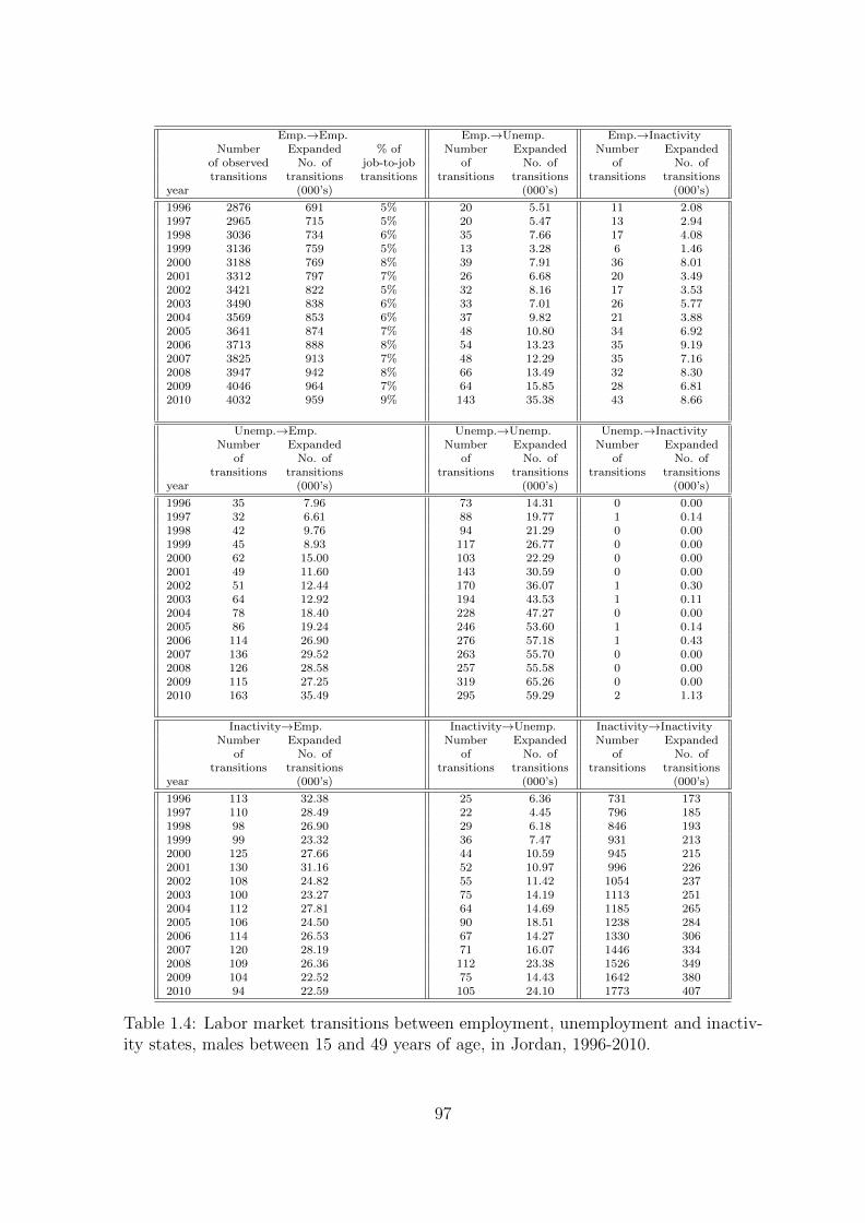
Emp.→Emp. Emp.→Unemp. Emp.→InactivityNumber Expanded % of Number Expanded Number Expanded

of observed No. of job-to-job of No. of of No. oftransitions transitions transitions transitions transitions transitions transitions

year (000’s) (000’s) (000’s)

1996 2876 691 5% 20 5.51 11 2.081997 2965 715 5% 20 5.47 13 2.941998 3036 734 6% 35 7.66 17 4.081999 3136 759 5% 13 3.28 6 1.462000 3188 769 8% 39 7.91 36 8.012001 3312 797 7% 26 6.68 20 3.492002 3421 822 5% 32 8.16 17 3.532003 3490 838 6% 33 7.01 26 5.772004 3569 853 6% 37 9.82 21 3.882005 3641 874 7% 48 10.80 34 6.922006 3713 888 8% 54 13.23 35 9.192007 3825 913 7% 48 12.29 35 7.162008 3947 942 8% 66 13.49 32 8.302009 4046 964 7% 64 15.85 28 6.812010 4032 959 9% 143 35.38 43 8.66

Unemp.→Emp. Unemp.→Unemp. Unemp.→InactivityNumber Expanded Number Expanded Number Expanded

of No. of of No. of of No. oftransitions transitions transitions transitions transitions transitions

year (000’s) (000’s) (000’s)

1996 35 7.96 73 14.31 0 0.001997 32 6.61 88 19.77 1 0.141998 42 9.76 94 21.29 0 0.001999 45 8.93 117 26.77 0 0.002000 62 15.00 103 22.29 0 0.002001 49 11.60 143 30.59 0 0.002002 51 12.44 170 36.07 1 0.302003 64 12.92 194 43.53 1 0.112004 78 18.40 228 47.27 0 0.002005 86 19.24 246 53.60 1 0.142006 114 26.90 276 57.18 1 0.432007 136 29.52 263 55.70 0 0.002008 126 28.58 257 55.58 0 0.002009 115 27.25 319 65.26 0 0.002010 163 35.49 295 59.29 2 1.13

Inactivity→Emp. Inactivity→Unemp. Inactivity→InactivityNumber Expanded Number Expanded Number Expanded

of No. of of No. of of No. oftransitions transitions transitions transitions transitions transitions

year (000’s) (000’s) (000’s)

1996 113 32.38 25 6.36 731 1731997 110 28.49 22 4.45 796 1851998 98 26.90 29 6.18 846 1931999 99 23.32 36 7.47 931 2132000 125 27.66 44 10.59 945 2152001 130 31.16 52 10.97 996 2262002 108 24.82 55 11.42 1054 2372003 100 23.27 75 14.19 1113 2512004 112 27.81 64 14.69 1185 2652005 106 24.50 90 18.51 1238 2842006 114 26.53 67 14.27 1330 3062007 120 28.19 71 16.07 1446 3342008 109 26.36 112 23.38 1526 3492009 104 22.52 75 14.43 1642 3802010 94 22.59 105 24.10 1773 407

Table 1.4: Labor market transitions between employment, unemployment and inactiv-ity states, males between 15 and 49 years of age, in Jordan, 1996-2010.

97

Emp.→Emp. Emp.→Unemp. Emp.→InactivityNumber Expanded % of Number Expanded Number Expanded

of observed No. of job-to-job of No. of of No. oftransitions transitions transitions transitions transitions transitions transitions

year (000’s) (000’s) (000’s)

1996 468 114 5% 1 0.32 13 3.241997 489 118 2% 3 0.83 17 5.411998 519 126 3% 4 1.02 14 3.001999 529 128 3% 3 0.86 25 7.612000 541 130 5% 3 1.23 36 8.972001 560 135 7% 4 0.72 32 8.112002 585 141 5% 10 3.38 24 5.212003 607 144 4% 8 1.90 29 7.562004 627 150 5% 7 2.03 40 9.642005 639 151 5% 9 2.10 45 11.802006 677 161 5% 8 1.43 33 9.282007 716 168 7% 9 2.46 40 11.252008 737 174 4% 15 3.93 33 7.782009 807 189 4% 9 2.54 33 8.472010 814 191 5% 17 4.05 47 11.52

Unemp.→Emp. Unemp.→Unemp. Unemp.→InactivityNumber Expanded Number Expanded Number Expanded

of No. of of No. of of No. oftransitions transitions transitions transitions transitions transitions

year (000’s) (000’s) (000’s)

1996 17 4.68 48 10.82 0 0.001997 15 3.06 52 11.44 1 0.151998 5 1.13 60 13.22 1 0.121999 13 2.87 64 14.26 0 0.002000 13 3.80 67 14.35 0 0.002001 18 3.73 61 13.35 0 0.002002 16 3.28 68 15.03 0 0.002003 16 3.64 74 17.64 1 0.312004 15 3.65 90 21.55 2 0.742005 24 6.72 105 23.67 0 0.002006 37 9.19 107 23.64 0 0.002007 33 8.90 126 25.46 0 0.002008 53 11.87 140 26.12 3 1.002009 39 7.79 198 36.23 1 0.112010 53 11.25 239 45.31 0 0.00

Inactivity→Emp. Inactivity→Unemp. Inactivity→InactivityNumber Expanded Number Expanded Number Expanded

of No. of of No. of of No. oftransitions transitions transitions transitions transitions transitions

year (000’s) (000’s) (000’s)

1996 28 6.84 17 3.18 3500 8181997 37 10.12 12 2.43 3618 8471998 35 9.91 13 2.87 3710 8671999 47 12.84 13 3.03 3825 8862000 51 12.92 9 1.49 3946 9172001 43 11.22 18 3.94 4087 9482002 45 9.88 13 3.19 4241 9832003 55 14.37 25 6.39 4357 10092004 56 12.70 32 6.81 4501 10452005 60 15.31 30 7.06 4652 10742006 58 13.34 42 8.66 4785 11042007 43 11.09 61 11.07 4926 11372008 67 15.92 83 14.07 5064 11762009 45 13.64 85 17.80 5237 12132010 45 10.38 104 22.27 5325 1229

Table 1.5: Labor market transitions between employment, unemployment and inactiv-ity states, females between 15 and 49 years of age, in Jordan, 1996-2010.

98

Chapter 2

Comparing Retrospective and Panel

Data Collection Methods to Assess

Labor Market Dynamics in Egypt 1

2.1 Introduction

The analysis of labor market dynamics requires the availability of data about the

same individuals at multiple points in time. This kind of data allows for the examina-

tion of flows between different labor market states rather than simply assessing labor

market stocks over time, which is what is usually possible with cross-sectional data.

Data about the same individuals over time can either be in the form of panel data,

where individuals are visited and interviewed multiple times over the course of several

months or years, or retrospective data, where individuals are asked about their past la-

bor market trajectories at one point in time. Although both methods of data collection

suffer from different kinds of measurement errors, panel data are often deemed superior

because they minimize recall error, which could be substantial in retrospective data.

Panel data, however, are expensive and difficult to collect and are, therefore, rarely

available to researchers in developing countries. If available, they are generally not col-

lected frequently enough to observe complete labor market trajectories and transitions.

1This chapter is mainly based on work conducted jointly with Ragui Assaad and Caroline Krafft(Assaad, Krafft, and Yassine, 2015).

99

It is therefore useful to examine how well retrospective data perform in assessing labor

market dynamics and the extent to which analyses that depend on them conform to

results obtained from panel data.

It is well known that retrospective data suffer from problems such as difficulties

in recalling dates or even that certain events occurred at all (Artola and Bell (2001);

Bound, Brown, and Mathiowetz (2001); Magnac and Visser (1999)). Panel data, that

is data that are collected contemporaneously at different points in time for the same

individual, are unlikely to suffer from recall errors but may have other problems. Be-

cause they are collected at discrete points in time, they only provide information at

those points in time and not on the course of events between those points (Blossfeld,

Golsch, and Rohwer, 2012). Moreover, panel data can suffer from sample attrition

and misclassification errors (Artola and Bell, 2001). They can also suffer from the

fact that individuals may be unwilling to accurately report their current status due

to fear of taxation or other government interference. Due to potential problems with

both retrospective (as has been discussed in chapter 1) and panel data, it is worth-

while to compare results on basic indicators related to labor market dynamics from

retrospective and panel data on the same sample of individuals, in order to determine

the conditions under which they provide similar or substantially different results. To

date, no study has undertaken such a comparison in the Middle East and North Africa

(MENA) region. This paper takes advantage of a unique opportunity to undertake

such a comparison, where both panel and retrospective data are available for the same

individuals in the Egypt Labor Market Panel Survey (ELMPS). Three waves of the

ELMPS were carried out by the Economic Research Forum (ERF) in 1998, 2006 and

2012. All three waves of the ELMPS contain both contemporaneous and retrospective

data, including detailed labor market histories for all individuals 15 and older who have

ever worked as well as other life course variables. Not only do the reference periods

of the retrospective data overlap with the dates of the previous waves of the survey,

allowing for comparisons of retrospective and panel data at the same point in time, but

the retrospective periods from different waves of the survey overlap with each other

as well, allowing for comparison of past events in one wave with the same events as

captured in another wave.

100

In this paper we assess the soundness of both the distribution of past statuses and

transitions among them obtained from the two sources of data. Specifically, we (i)

assess the consistency of reporting of time-invariant characteristics in different waves of

the panel, (ii) compare the retrospective and panel data results on past labor market

statuses, including the estimation of multivariate models of the determinants of align-

ment between the two data sources, (iv) assess the consistency of estimates of labor

market transition rates across two specific dates by comparing panel and retrospective

data, (v) assess the consistency of estimates of the level and trends of annual labor

market transition rates across retrospective data from two different waves of the sur-

vey, and (vi) assess whether retrospective data can provide accurate trends of labor

market aggregates, such as employment-to-population ratios and unemployment rates.

The rest of the paper is organized as follows. Section 2 reviews the theory and

past evidence on measurement error in contemporaneous and recalled data. Section

3 includes a discussion of our data source and methods of analysis. Section 4 lays

out all our findings on the various comparisons we make and section 5 concludes with

recommendations as to what kinds of information can be reliably collected using ret-

rospective questions, how to improve retrospective data collection strategies to obtain

more reliable information, and potential methods for correcting measurement errors.

2.2 Theories and Past Evidence on Measurement

Problems in Current and Recalled Data

Whether labor market states and transitions can be accurately represented by cur-

rent (contemporaneous panel) or recalled (retrospective) data is essentially an issue of

measurement error. Surveys are attempting to measure a certain phenomenon such as

the current labor market status, or the date of the first job but the data reported may

be erroneous. The literature on measurement error suggests a wide variety of issues

that might contribute to measurement errors in both current and recalled information.

This section begins with a summary of the threats to research created by measurement

error, then discusses some of the key issues that contribute to measurement error in

current and recalled data. The section concludes with the evidence to date character-

101

izing these problems, with a particular focus on findings relating to labor markets in

developing countries.

2.2.1 The Implications of Measurement Errors

The implications of measurement error depend substantially on the nature of the

problems. Truly random errors in continuous variables sometimes do not present a

substantial problem to research, as they will not affect estimates of key statistics such

as means. In estimating linear regression models with a mis-measured continuous de-

pendent variable, y, so long as the measurement error in y is random, results will not be

biased (although standard errors will be increased) (Bound, Brown, and Mathiowetz,

2001). Random errors in an explanatory variable, x, will downward-bias or attenu-

ate the estimated coefficient on x in a linear regression model (Bound, Brown, and

Mathiowetz, 2001).

Random errors in categorical or binary variables are more problematic. For example,

if a variable is binary, such as whether or not an individual is employed, an error must

always be the opposite of the true value. That is, if the true value of some y∗ = 1,

then the measured value, y, may be 0 or 1, and it is always the case that y − y∗ ≤ 0.

Likewise if y∗ = 0, then the measured value, y, may be 0 or 1, and it is always the case

that y − y∗ ≥ 0. Thus, the correlation between the true value and the error is always

negative (Bound, Brown, and Mathiowetz, 2001). In the case of even random errors

in a limited (categorical, binary) dependent variable, unlike in the continuous case,

regression results will be biased downwards (attenuated). As in the continuous variable

case, when the mis-measured variable is an independent, explanatory variable, this

will lead to downward-biased (attenuated) estimates (Bound, Brown, and Mathiowetz,

2001).

Often, measurement errors are not random, but are instead systematic that is, re-

lated to characteristics or covariates. In this case, measurement errors will bias both

basic statistics and regression coefficients in complex ways (Bound, Brown, and Math-

iowetz, 2001). For instance, when studying the incomes of the self-employed, individuals

with more education may keep accounting books and be able to more accurately report

their incomes. If less educated individuals systematically under-report their incomes,

102

this will systematically bias a regression estimating the relationship between years of

education and income.

2.2.2 Why do measurement errors occur?

A variety of different processes can generate errors in data. Measurement problems

can be either unintentional or intentional misreporting, and we discuss here a number

of the processes that contribute to these different types of misreporting.

The process of respondents providing information to survey data collectors can suffer

from a number of errors. The question answering process for a respondent requires, first,

comprehension of the question, the recollection of the information from one’s memory,

comparing the retrieved information with the original question, and communicating

this information to an enumerator (Bound, Brown, and Mathiowetz, 2001). A large

body of literature focuses on the recall or retrieval process and the nature of errors in

recall. These are particularly likely to be affected by the recall period. That is, the

longer the recall period (the further back in time the event in question is), the more

likely that respondents will report with error, although the extent to which this is a

problem varies substantially over studies of different outcomes (Bound, Brown, and

Mathiowetz, 2001).

In reporting the dates of various events, the misreporting of dates may be a function

of how far back in time the event occurred. Respondents are more likely to move forward

the date (“forward telescoping”) an event that has a short reference period (a few weeks)

while respondents are more likely to move back in time an event that occurred a year

or more in the past (Bound, Brown, and Mathiowetz, 2001). Studies of panel data on

dates have identified what is commonly referred to as a “seam effect”, i.e. excessive

numbers of changes at the “seam” between one study period and the next (Bound,

Brown, and Mathiowetz, 2001).

The “salience” or importance of events may affect the accuracy with which they

are reported (Bound, Brown, and Mathiowetz (2001); Judge and Schechter (2009)).

For instance, unemployment spells of only a few weeks may be of lower salience than

unemployment spells that last a year and therefore be more likely to be forgotten.

Individuals may forget when, or even whether, certain events occurred at all. If indi-

103

viduals do remember events, they may not readily remember the exact timing of events.

This leads to measurement errors such as “heaping”, where individuals tend to report

certain numbers as responses (Roberts and Brewer, 2001). For instance, respondents

often report adult ages in years in multiples of 5 or child ages in months rounded to

the nearest year or half year (Heitjan and Rubin (1990); Roberts and Brewer (2001)).

Question and questionnaire design can play an important role in whether respondent

errors occur. Identifying the best respondent within a household, deciding on the level

of aggregation for data, and asking for information in the most appropriate units and

for the most appropriate reference period are important elements of design that will

affect the accuracy of measurement (Grosh and Glewwe (2000); Puetz, Von Braun, and

Puetz (1993)). As well as unintentional errors, primarily due to difficulties accurately

recollecting information about states and events, responses in surveys may suffer from

intentional respondent misreporting. Particularly for topics that relate to behaviors

or states that have strong connotations of social (un)desirability, such as the inten-

tion to send children to school or the receipt of charity, respondents may misreport.

Under-reporting will occur for socially undesirable phenomena, and over-reporting for

desirable phenomena, generating “social desirability bias” (Bound, Brown, and Math-

iowetz, 2001).

As well as respondents providing inaccurate information, interviewer practices and

data processing may generate inaccurate information. Differences arise in the quality

of government-collected and academic researcher-collected data (Judge and Schechter,

2009), which may be due to differences in the qualities and characteristics of inter-

viewers and data processing. As well as subtler issues such as interviewers with poor

training and weak incentives (Puetz, Von Braun, and Puetz, 1993), outright fieldworker

fraud may occur. Such fraud is particularly likely to bias panel data estimates (Finn

and Ranchhod, 2013). Quality control during data collection can help address such

issues (Puetz, Von Braun, and Puetz, 1993).

2.2.3 Evidence on the extent of errors in survey data

The Malaysian Family Life Survey (MFLS), with panel data 12 years apart and

substantial retrospective elements, suggests some of the issues that may occur in devel-

104

oping country data. The survey focused on issues of fertility and health and therefore

targeted ever-married women. The MFLS also collected life histories on issues such

as employment, migration, and marriage. The findings demonstrate that substantial

errors can occur, but also that reporting of retrospective events can be quite accurate.

For instance, while 95% of the ever-married sample reported being currently married in

the first wave of the survey in 1976, twelve years later, only 84% of panel respondents

reported in 1988 that they had been married in 1976. This difference is substantial and

statistically significant. However, the same rate of mortality for children born prior

to 1976 results from both the 1976 and 1988 interviews (Beckett, Da Vanzo, Sastry,

Panis, and Peterson, 2001). The level of detail in the question affected the accuracy

of reporting as well; for instance, agreement was much higher in reporting whether

a child was ever breastfed than the duration of breastfeeding. The salience of events

also mattered; women reported inter-district moves (a more substantial move) more

consistently in 1976 compared to 1988 than intra-district moves (only 80% of the rate

of moves prior to 1976 was reported in 1988). Substantial “blurring” of dates also oc-

curred, with mothers not reporting exact months or years for children’s births when

they were relatively further back in time across the two waves. Quantities were more

likely to be rounded (akin to heaping), with rounding increasing with the length of

recall. Studies have found different reporting errors with the MFLS to be related to

respondent characteristics (Beckett, Da Vanzo, Sastry, Panis, and Peterson, 2001).

A number of studies have also been conducted on measurement of income, assets,

and consumption. A study of boat-based fisherman in India looked at self-reported

income over 34 months and compared it to administrative data from the fishermen

society (De Nicola and Gine, 2014). The study found that the mean of income is

maintained but variance reduced when going back 24 months. Findings suggested

that boat owners reverted to inference, i.e. reporting mean income, as recall periods

lengthened. Asking about the date of boat purchase directly elicited responses of similar

quality to asking in relation to time cues (anchoring) important to the respondent;

using unimportant time cues generated substantially worse results. The timing of the

question within the survey did not, however, affect results (De Nicola and Gine, 2014).

Using data from Africa, Beegle, Carletto, and Himelein (2012) look for recall bias

105

in agricultural data from three household surveys in African countries. Agricultural

data usually refer to an agricultural season or year, and may be subject to recall bias of

varying degrees depending on, for example, the time since harvest. The authors regress

information on harvest sales and input use on the time elapsed between harvest and

interview. They find little recall bias, although more salient events may be reported

more accurately.

As well as examining income data, a number of studies have examined recall er-

rors in expenditure and consumption data. Using household survey from Vietnam and

resurveying respondents, Hiroyuki, Yasuyuki, and Mari (2010) find that questions on

total rather than categorical expenditure suffer less recall bias. They also find that

errors are systematically related to household size, and that errors are more serious

for goods produced for own consumption than purchased goods. Errors tend to be

mean-reverting, which will bias coefficients downward. Beegle, De Weerdt, Friedman,

and Gibson (2012) compare eight different methods for measuring household consump-

tion, comparing to a benchmark of personal diary use other diary and retrospective

approaches. Recall is lower for other approaches than diaries, with particularly acute

problems for poorer, larger, and less educated households.

Using United States data including a longitudinal survey, long-term retrospective re-

call data, and company records, comparisons demonstrated that the means of earnings

were very similar in retrospective responses and company records. However, transitory

variations were under-reported, generating another case of mean-reverting errors (Gib-

son and Kim, 2010). In a similar vein to our work on labor market dynamics, Dercon

and Shapiro (2007) examine the role of measurement problems in poverty dynamics in

panel data. They review past work on poverty mobility and discuss several key errors

that are also relevant in our work: (1) inaccurate measures of income or consumption

(2) price deflation and (3) mismatching of households over survey waves.

One way to test for problems in survey data is using Benford’s law, which de-

scribes the distribution of first significant digits that should occur in large sets of data.

Comparisons of observed distributions with the distributions implied by Benford’s law

allows for an assessment of respondent and enumerator response problems (Finn and

Ranchhod (2013); Judge and Schechter (2009)). An application of Benford’s law to

106

multiple surveys noted that certain questions were particularly likely to suffer from

response irregularities and that there were quality differences between government and

academic survey data (Judge and Schechter, 2009). Applications of Benford’s law and

other methods for detecting fieldworker fabrication of data in South Africa’s National

Income Dynamics study found around 7% of the sample was affected. While cross-

sectional estimation was not substantially affected by fabrication, panel estimators

were (Finn and Ranchhod, 2013).

2.3 Data and Methods

2.3.1 Data Sources

To compare results from panel and retrospective data, it is necessary to have a

survey that collects contemporaneous data at different points in time as well as retro-

spective data for the same individuals. The only survey that meets these criteria in

the MENA region is the Egypt Labor Market Panel Survey (ELMPS). With waves in

1998, 2006, and 2012, it is possible to use the ELMPS to compare retrospective and

panel data over multiple periods. The ELMPS is a nationally representative household

survey with detailed modules on current and past labor market statuses. Of the origi-

nal 23,997 individuals interviewed in 1998, 13,218 (55.1%) were re-interviewed in both

2006 and 2012. Of the 37,140 individuals interviewed in 2006, 18,770 (77.5%) were

re-interviewed in 2012 2. A retrospective panel of annual statuses is constructed from

retrospective data in each wave and compared to panel and retrospective data from

previous waves. Reporting of time invariant information, such as parent’s education,

is also compared based on reports in different waves of the survey.

A particularly important element of our analyses relies on the labor market history

section of the ELMPS surveys, which is administered to all individuals 15 and older

who ever worked. In 2012, this section asks for the start and end dates (year, month)

and characteristics of labor market statuses lasting six months or more from the time

2See Assaad and Roushdy (2009) and Assaad and Krafft (2013) for a discussion of attrition fromthe various waves of the ELMPS.

107

the individual exited school 3. A status is defined as any labor market state lasting

six months or more, be it employment, unemployment or out of the labor force. If

the individual is employed in that status, she or he is asked about the details of such

employment, including employment status (wage work, self-employment, etc.), sector

of employment, occupation, economic activity, incidence of a formal contract and/or

social insurance coverage, location of work, and reason for changing the status. The

questionnaire inquires about the first four statuses lasting six months or more. Statuses

of less than six months are dropped and if four statuses are not enough to reach the

current status, the fifth and later statuses are also dropped. However, the total number

of employment spells and their start and end dates can be obtained from the life events

calendar section of the questionnaire. In addition to the first four statuses and the cur-

rent status, which is obtained elsewhere in the questionnaire, the questionnaire inquires

whether the individual’s current status (in early 2012) was different from their status

in the month prior to the January 25th 2011 revolution. If it was, the questionnaire

elicits information about the individual’s status during that month.

It is important to note that in the preceding waves of the ELMPS survey (1998

and 2006), the labor market history questions were sequenced differently. Specifically,

these waves of the survey used a reverse chronological order in eliciting labor market

trajectories as compared to the chronological method used in 2012. In 1998 and 2006,

the questionnaire first inquired about the current labor market status, then the previous

status and the status previous to that, collecting information about the date of start of

each of these statuses. In addition, information was collected in a separate part of the

questionnaire about the first job in which the individual was engaged for a period of

more than six months. Unlike the 2012 wave, the 1998 and 2006 waves did not contain

a life events calendar and therefore no information on the total number of primary

jobs the individual engaged over his/her lifetime. This questionnaire design implies

that initial unemployment and out of labor force states could be missed, as well as

employment states between the first job and the pre-previous status.

3For individuals who never went to school, the retrospective period starts at age 6.

108

2.3.2 Methods

To compare retrospective and panel data, the retrospective data were mapped on to

panel data from previous waves in such a way that retrospective and current information

is available for the same individual at the same point in time. We then draw on the

econometric literature on measurement error to assess and compare the data sources

and suggest possible corrections to account for measurement error (Black, Berger, and

Scott (2000); Bound, Brown, and Mathiowetz (2001); Carroll, Ruppert, Stefanski, and

Crainiceanu (2006); Fuller (2009); Magnac and Visser (1999)).

As a first check on the accuracy of the panel data, we begin by comparing the

consistency of time invariant information across different waves of the panel. We do

that for own education for adults 30-54 in 1998, father’s sector of work when the

individual was 15 years of age, and recalled costs of marriage. We then compare labor

market statuses at a given point in time (1998 and 2006) across retrospective and panel

data to assess the accuracy of recall and identify statuses that are particularly prone

to erroneous recall. We subsequently estimate a multivariate model of the probability

of alignment in labor market status between the two kinds of data as a function of

individual characteristics, whether the information was elicited from the individual

him/herself or a proxy respondent, the nature of the past employment status itself,

and the contemporaneous employment status in 2012.

The next step is to assess the consistency of reporting of labor market transitions

in retrospective and panel data. To do this, we convert the retrospective data into an

annual retrospective panel, which contains information about the main labor market

variables every year since the individual exited school for the first time. Using this

retrospective panel we calculate the rate of change in employment status from 1998

to 2006 using the respective waves of the panel for those dates to the rates of change

over the same period as reported by the 2012 retrospective data. We then move to

comparing annual transition rates derived from the retrospective data in different waves

of the survey.

In examining labor market transitions, we examine two types of transitions of par-

ticular interest to the study of labor market dynamics: transitions among employment,

unemployment and out-of-labor-force states, and job-to-job transitions among the em-

109

ployed. Within the first type, we include job-finding rates for the unemployed and those

out of the labor force, and separation rates from employment to either unemployment

or out of the labor force. The second type includes two-way transitions across different

types of jobs, such as public and private employment and wage and non-wage work.

We examine how different waves of the retrospective data generate transition rates, by

type of transition. Finally, we revisit the question of whether the levels and trends in

important labor market ratios of stocks, such as the employment-to-population ratio

and the unemployment rate, can be accurately assessed using the retrospective data,

by comparing across different waves of retrospective data and between them and con-

temporaneous sources of these data, such as the official labor force survey.

2.4 Findings

2.4.1 Consistency of reporting of time-invariant information

across different waves of a panel survey

Own Education for Adults

The accuracy of the characteristics individuals report in any survey, such as their

age, education, or labor market characteristics, plays an important role in researchers’

ability to accurately describe economies and labor markets. Often researchers are

focusing on cross-sectional, contemporaneous labor market characteristics. Comparing

how individuals report static characteristics over time can help researchers understand

how accurately contemporaneous characteristics are reported in cross-sectional data.

Because the ELMPS is a panel, we can compare characteristics that should remain

unchanged, such as education (for adults) as reported in different waves of the survey

in order to assess their accuracy.

Figure 2.1 compares the reporting of education in 1998 with that in 20064 for

individuals ages 30-54 in 1998. It is important to keep in mind that either the 1998 or

the 2006 response could be inaccurate when they disagree, or both could be consistent

4Comparisons are not made with 2012 because, to reduce the burden of responding to the survey,respondents who answered educational questions in 2006 and had no change in education status werenot re-interviewed about education.

110

(but still inaccurate) over time. Education is examined categorically, in terms of eight

different categories. Overall, 79% of responses are the same over time, but there is

substantial variation in terms of which education categories are reported consistently.

For instance, 90% of those who reported being illiterate in 1998 report being illiterate

again in 2006. The remainder primarily report being able to read and write but having

no education certificate (7%), which could be a genuine change in literacy, or having

primary education (3%). The ability to read and write appears to be the most poorly

reported, with only 34% of those reporting they could read and write but having no

education certificate in 1998 reporting the same status in 2006. The most common

response in 2006 for this group is being illiterate, which may represent a genuine decay

in reading and writing ability. In general, when reporting is different, the reported

alternative is usually a proximate level of education. For instance, 20% of those who

reported general secondary in 1998 then report they attended vocational secondary in

20065. Likewise 22% of those who reported post-secondary education in 1998 reported

being vocational secondary graduates in 2006. Since the distinction is not always

clear between special five-year vocational secondary programs and three-year vocational

secondary plus two-year post-secondary programs, this may contribute to the lower

consistency.

Figure 2.1: Education (8 categories) as reported in 1998 vs. 2006, Ages 30-54 in 1998

Source: Authors’ calculations based on ELMPS 1998 and ELMPS 2006Notes: See Table 2.4 for values underlying figure.

5Smaller categories, such as general secondary, may suffer from more mis-reporting due to theirtiny size. For instance, if random typos are uniformly distributed across the categories, more responsesin the smallest categories are likely to be errors.

111

Although every effort is made to collect data from the individual him or herself, one

dimension of data collection that is likely to affect measurement problems is whether or

not the respondent is, in fact, the individual in question. Data consistency can also be

assessed along this dimension of reporting. We compare the education status in 1998

and 2006 of individuals who were consistently responding for themselves and those

who were not consistently responding for themselves6. Among individuals in the panel

who were 30-54 in 1998, 71.3% reported for themselves in both waves (94.9% in 1998

and 75.7% in 2006). When the individual in question is consistently the respondent,

there is a slight (but not dramatic) improvement in the consistency of data. There is

only a one percentage point increase in consistency of illiteracy, primary, and university

reporting, but larger improvements in read and write (5 percentage points), preparatory

(6 percentage points), vocational secondary (6 percentage points) and post-secondary

(4 percentage points) reporting.

Figure 2.2: Education (8 categories) as reported in 1998 vs. 2006, by respondent, ages30-54 in 1998

Source: Authors’ calculations based on ELMPS 1998 and ELMPS 2006Notes: See Table 2.5 for values underlying figure.

Creating less finely aggregated categories, such as only four education levels, can

6When individuals were not consistently responding for themselves, it is possible that the sameindividual was responding in their place in both waves (i.e. a spouse) but the data does not allow usto determine whether this is so.

112

Figure 2.3: Education (4 categories) as reported in 1998 vs. 2006, Ages 30-54 in 1998

Source: Authors’ calculations based on ELMPS 1998 and ELMPS 2006Notes: See Table 2.6 for values underlying figure.

lead to more consistency in reporting (Figure 2.3). Combining illiterate and read &

write leads to a category that is consistently reported 93% of the time. Combining

primary and preparatory education into a single category leads to 76% of respondents

reporting consistently over time. A category that combines general, vocational and

post-secondary into the definition “secondary” is 91% accurately reported over time.

University and above was consistently reported as 94% over the two waves. Overall, it

is clear that using more aggregated categories leads to more consistent reporting; more

detailed categories should be viewed with some caution (particularly read and write

and general secondary).

Father’s sector of work

Particularly for analyzing patterns across generations, it is necessary to gather in-

formation on parents’ characteristics, even if they are not present in the respondent’s

household. The ELMPS collects information on father’s characteristics when the re-

spondent was age 15 from respondents when the father is not in the household. Figure

2.4 shows the consistency of responses over time (2006 versus 2012) among respon-

dents age 30-54 whose father was not present in 2006 or 2012. Approximately 71%

of respondents who reported their father worked in government in 2006 then report

that their father worked in government in 2012, while 7% said their father worked in

public enterprise and 22% worked in the private sector. Private sector work is rela-

113

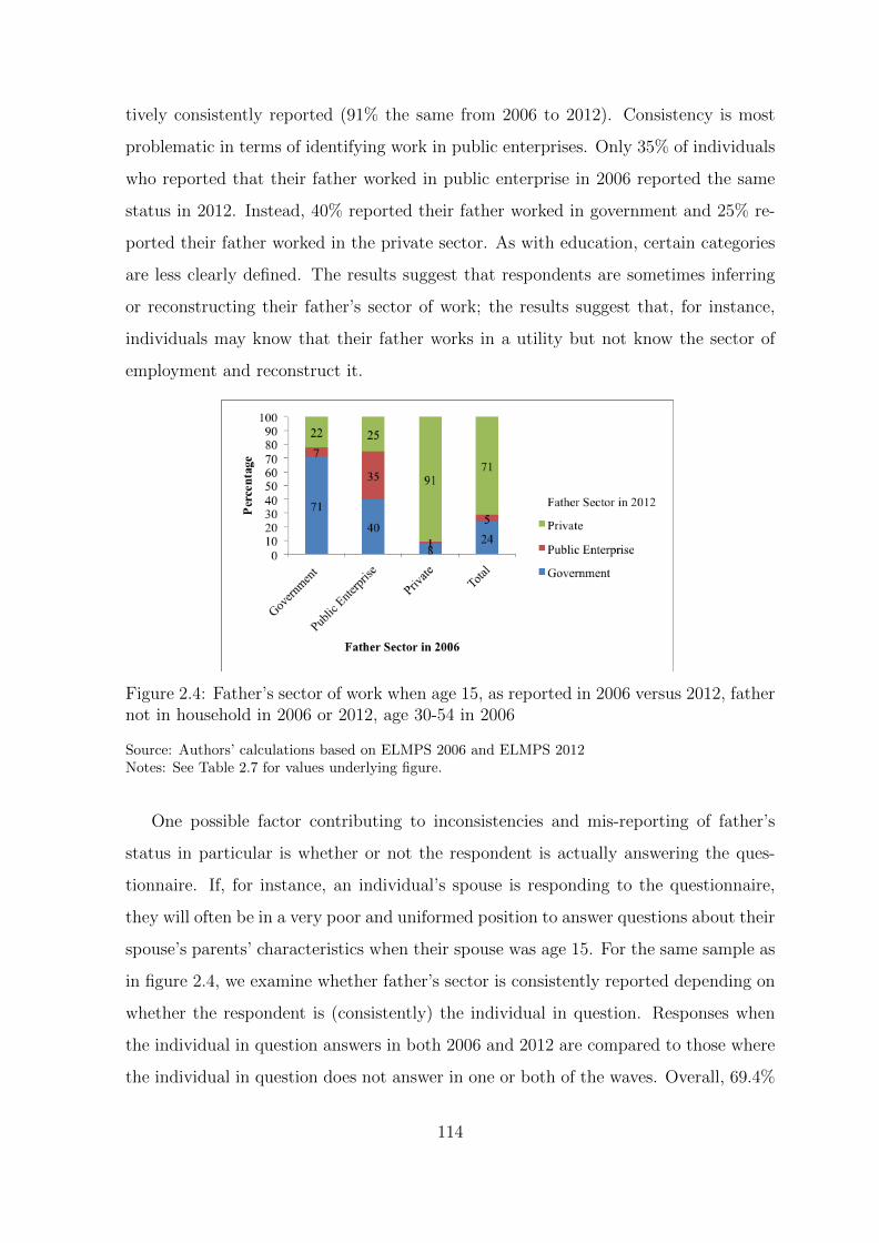
tively consistently reported (91% the same from 2006 to 2012). Consistency is most

problematic in terms of identifying work in public enterprises. Only 35% of individuals

who reported that their father worked in public enterprise in 2006 reported the same

status in 2012. Instead, 40% reported their father worked in government and 25% re-

ported their father worked in the private sector. As with education, certain categories

are less clearly defined. The results suggest that respondents are sometimes inferring

or reconstructing their father’s sector of work; the results suggest that, for instance,

individuals may know that their father works in a utility but not know the sector of

employment and reconstruct it.

Figure 2.4: Father’s sector of work when age 15, as reported in 2006 versus 2012, fathernot in household in 2006 or 2012, age 30-54 in 2006

Source: Authors’ calculations based on ELMPS 2006 and ELMPS 2012Notes: See Table 2.7 for values underlying figure.

One possible factor contributing to inconsistencies and mis-reporting of father’s

status in particular is whether or not the respondent is actually answering the ques-

tionnaire. If, for instance, an individual’s spouse is responding to the questionnaire,

they will often be in a very poor and uniformed position to answer questions about their

spouse’s parents’ characteristics when their spouse was age 15. For the same sample as

in figure 2.4, we examine whether father’s sector is consistently reported depending on

whether the respondent is (consistently) the individual in question. Responses when

the individual in question answers in both 2006 and 2012 are compared to those where

the individual in question does not answer in one or both of the waves. Overall, 69.4%

114

Figure 2.5: Father’s sector of work when age 15, as reported in 2006 versus 2012, byrespondent, father not in household in 2006 or 2012, age 30-54 in 2006

Source: Authors’ calculations based on ELMPS 2006 and ELMPS 2012Notes: See Table 2.8 and Table 2.9 for values underlying figure.

of individuals in the sample were consistently reporting for themselves. The patterns

of reporting by respondent are presented in figure 2.5. Having the respondent consis-

tently be the individual in question improves the results at most a little. Reporting of

private sector work and public sector work is nearly identical. Only in regards to pub-

lic enterprise work does having the respondent consistently report appreciably improve

consistency, 39% reporting public enterprise in both waves when consistently reported

by the respondent and 33% otherwise.

Recalled costs of Marriage

Understanding the investments individuals have made over time often requires ask-

ing about past outlays of expenditure. Individuals are expected to provide the costs of

expenditures and investments when they occurred. However, especially when individ-

uals are inferring or reconstructing the value of an investment, for instance inferring

the cost of their housing at the time of marriage based on their current cost or value of

housing, this can cause problems in assessing trends over time. Essentially, individuals

may (fully or partially) update past expenditures from nominal to real terms. Figure

115

2.6 shows the trends in the total costs of marriage over time for individuals who were

married in 2012 and present in both the 2006 and 2012 waves (they may not have yet

been married). Marriage is an enormous investment for young people and their families,

and the cost of marriage and its trends in Egypt and the MENA region are the sub-

ject of substantial concern and discussion (Assaad and Krafft (2015a,2015b); Assaad

and Ramadan (2008); Dhillon, Dyer, and Yousef (2009); Salem (no date, 2015,2012);

Singerman and Ibrahim (2001); Singerman (2007)). The figure shows both the nominal

(reported) costs and the real (inflated to 2012 LE) costs by year, as reported in both

2006 and 2012. Nominal marriage costs are clearly rising over time using both the

2006 and 2012 data, and the difference between those reports (when they overlap) may

be due to inflation. Using the 2006 data and 2012 prices, it appears that from 2000

to 2006, marriage costs were flat or slightly declining, and averaged around 60,000 to

70,000 LE. Using the 2012 data and 2012 prices, looking at the same respondents re-

ported marriage costs from 2000 to 2006, it appears marriage costs were flat or slightly

declining, but averaged around 90,000 LE. This is clearly inconsistent with what was

reported in 2006, even when updated to 2012 prices. It appears individuals are partially

(but not fully) updating nominal costs into real terms, as nominal costs for 2000-2006

as reported in 2012 are too high compared to 2006 nominal costs, but real costs for

2000-2006 as reported and then inflated using 2012 data are too high compared to 2006

reports updated into 2012 prices. Additionally, further investigation suggests different

elements of marriage costs are updated differentially, likely related to how easy they

are to recall or reconstruct.

Continuing to examine the 2012 data out to 2012 in real terms, it appears that

marriage costs have fallen substantially over time, from around 90,000 in 2000-2006 to

around 60,000-70,000 by 2012. This implies the cost of marriage over the 2000-2012

period decreased almost a third. By this comparison, marriage costs are falling over

time. However, looking back at marriage costs as reported in 2001-2006, and updated

to 2012 terms, marriage costs have remained essentially constant, in the 60,000-70,000

range (in 2012 LE). This is evidence that, particularly when asked about events that

are now a number of years in the past, individuals may be inferring their value or

inflating into current terms. Thus suggests that retrospective data should not be used

116

Figure 2.6: Total Marriage Costs, as reported in 2006 versus 2012, respondents in bothwaves, answering marriage section in 2012 (may not yet have been married in 2006)

Source: Authors’ calculations based on ELMPS 2006 and ELMPS 2012.

to assess time trends for investments and financial outlays; repeated cross sections or

panel data are required. Comparing investments in the few years preceding a survey

wave to investments in the few years preceding different survey waves will be more

accurate for such cost data.

2.4.2 Comparing labor market statuses across retrospective

versus panel data

Alignment of labor market statuses in general

Individuals’ labor market statuses, namely whether they are out of the labor force,

unemployed, or employed, and if employed, their employment status, are at the heart

of labor market surveys. Both the accuracy of individuals’ contemporaneous statuses

and the accuracy of the labor market histories they report are of great interest. The

latter are particularly important for assessing labor market dynamics. This section first

assesses whether aggregate statistics vary by data source and then whether individuals

report consistently across contemporaneous and retrospective data.

Figure 2.7 presents aggregate labor market statistics by gender for 1998 and 2006

using both contemporaneous statistics from the waves of the panel and retrospective

reports from 2012 for those years. Notably, for males the aggregates from both the

retrospective and contemporaneous data are quite similar, with a few exceptions. Re-

117

porting of public sector work, private formal and informal regular wage workers, and

self-employment are fairly similar. Irregular wage work is differentially reported in the

retrospective data, which is likely because hours of work fluctuate over time; individuals

may remain at the same job over time, but report that it is irregular in 2012 and map

that back onto their status in previous years. Changes in regularity within the same

job are also not captured within the labor market history and are difficult to detect.

Employers are more likely to be reported in the contemporaneous than retrospective

data.

Figure 2.7: Labor market status, as reported contemporaneously for 1998 and 2006 andas reported retrospectively for those years from 2012 data, by sex, respondents ages30-54 in 2012 present in both waves

Source: Authors’ calculations based on ELMPS 1998, ELMPS 2006 and ELMPS 2012Notes: See Table 2.10 and Table 2.11 for values underlying figure.

For individuals 30-54 in 2012, their ages would have been approximately 24-48 in

2006 and approximately 16-40 in 1998. Thus, it is only in 1998 that many would have

been out of or transitioning into the labor force (unemployed). These statuses appear

to be under-reported in the retrospective data comparing 1998 contemporaneous data

to the retrospective data for 1998 from 2012. For instance, while 7% of males were

unemployed in 1998 contemporaneously, in the retrospective data only 2% of males

118

report being unemployed. Likewise in the 1998 contemporaneous data, more individuals

report being out of the labor force. There are so few females in a number of labor

market statuses that our assessment focuses primarily on the public sector, unpaid

family work, unemployed women, and women out of the labor force. Public sector

work is quite consistently reported in the aggregates, which may be due in part to the

stability of this employment status. Unpaid family work, which includes subsistence

work, is much more frequently reported in the contemporaneous data (6-10% across

years) than in retrospective data (3-4%). This may be in part because individuals are

only asked the labor market history in 2012 if they report having ever worked in market

work, and unpaid family workers may switch into and out of market work, sometimes

producing agricultural goods for their own subsistence and sometimes selling them on

the market. Unemployment is also more frequently reported in the contemporaneous

data than in the retrospective data. This is likely due to the fact that many women

who search for work never end up working (Assaad and Krafft, 2014) and thus are

not asked the questions in the labor market history. As a result of these patterns in

reporting employment, being out of the labor force is higher in the retrospective than

contemporaneous data for women.

A number of labor market statuses are particularly prone to misreporting over

time, comparing retrospective and contemporaneous data. Figure 2.8 presents the dis-

tribution of retrospective statuses going back from 2012 to various years by the status

reported contemporaneously from 2006 or 1998 for individuals 30-54 in 2012, by sex.

There also is somewhat greater inconsistency comparing 1998 statuses than 2006 sta-

tuses, which is likely due to recall deteriorating over time. While public sector employ-

ment tends to be reported quite consistently, other labor market statuses are frequently

not reported consistently. Formal private sector work tends to be more consistently re-

ported than informal work. Most reporting of wage work is consistent, but the type

of wage work is not consistently reported. Distinctions between self-employment and

being employers are likewise blurred. Those who were unemployed or out of the labor

force show a high degree of inconsistencies. Some of this may be because the duration

of these statuses is shorter, so the contemporaneous status may be off relative to the

status that is measured as predominant for the year. Females have a much higher

119

probability than males of reporting that they are out of the labor force (which is their

predominant status). Less formal forms of employment in the contemporaneous data,

such as being an employer, self-employment, and unpaid family work are particularly

likely to be reported as being out of the labor force. Being unemployed suffers from a

similar problem, likely, as mentioned earlier, due to the large share of women who are

unemployed but ultimately never find work. These patterns, as with education, suggest

a number of issues for analyzing labor market statuses and dynamics. For instance,

a category of private wage work, incorporating regular formal and informal and irreg-

ular workers would be more consistently reported than the disaggregated categories,

and transitions between regular/irregular and formal/informal may be poorly reported

over time. Self-employment and being an employer also often are mixed up, and might

be better combined into a single category. For females, retrospective data should be

treated with particular caution, as women may not report ever working when they have

done so, or report being out of the labor force when they were in fact working in the

private sector. Although it is not certain from the comparison of the contemporane-

ous and retrospective data which is correct, contemporaneous information on women’s

status shows greater differences from retrospective data than the same comparison for

men.

Using more aggregated categories of employment status leads to somewhat greater

consistency in responses. Figure 2.9 compares the distribution of retrospective statuses

going back from 2012 to various years of by the status reported contemporaneously

from 2006 or 1998, using only four categories: public, private wage, non-wage, and

not working. Public sector wage work continues to be the most consistently reported

category, as before. For males, private wage work is fairly consistently reported com-

paring 2012 retrospective statuses to 2006 (72%) and 1998 (66%). More males tended

to report that they were not working retrospectively who were working in private wage

work in 1998 (10%) than 2006 (3%). Only around half of those who reported being

non-wage workers in 1998 or 2006 reported the same status in the retrospective data

(55% for 2006 and 47% for 1998). Most of the remainder reported private sector wage

work. Although half (57%) of those who reported not working in the 1998 wave also

reported not working in the 2012 retrospective data for 1998. Despite the recall time

120

Figure 2.8: Labor market status, as reported in 1998 or 2006 versus 2012 retrospectivedata for 1998 or 2006, by sex, respondents ages 30-54 in 2012 present in both waves

Source: Authors’ calculations based on ELMPS 1998, ELMPS 2006 and ELMPS 2012Notes: See Table 2.12, Table 2.13, Table 2.14, and Table 2.15 for values underlying figure.

121

being shorter, there was less consistency between those who reported not working in

2006 and the 2012 recall data for 2006 (27% consistency). This may be because those

males 30-54 in 2012 were 16-40 in 1998, and therefore were more likely to have a long-

term status of not working (preceding entry into work for the first time). Those males

30-54 in 2012 were 24-48 in 2006, and so time spent not working would more likely

have been short in duration. Not working, for instance short spells of unemployment,

may not have even met the definition for a status lasting six months and therefore not

been included in the labor history.

Although aggregating labor market statuses causes some important improvements

in consistency across males’ labor market histories and contemporaneous statuses, there

is less improvement in consistency in females’ statuses, primarily because they fail to

report employment at all. Those in public sector work according to their 1998 or 2006

reporting do consistently report that in the retrospective data and those not working

according to the 1998 and 2006 waves report not working in the retrospective status.

However, less than half of those in private wage work in one wave reported this in their

retrospective data for 2012 (43% for 2006 and 24% for 1998). Consistent reporting of

non-wage work is even lower (27% for 2006 and 13% for 1998). The inconsistencies

are primarily due to individuals saying they were not working at the time. Further

examination of the data demonstrated that a key problem is detection of whether

women ever worked at all. Among the women examined, just two-thirds (67%) of

those who were identified in 2006 as engaging in market work reported that they ever

worked in 2012. Likewise just 73% of females who were identified as engaged in market

work in 1998 reported ever working in 2012. This was not a problem for men (<1%).

The problem was driven by women who were no longer working in 2012; all of those

working in 2012 were, of course, identified as having ever worked. However, among

women who were not working in 2012 but were working in 2006, only 16% reported

ever working in 2012. Among women who were not working in 2012 but were working

in 1998, only 18% reported ever working in 2012. Only those who report ever working

are asked the labor market history, and thus these women are considered to never have

worked and no labor market history data is collected.

We had initially expected substantially more consistent reporting of labor market

122

Figure 2.9: Collapsed labor market status, as reported in 1998 or 2006 versus 2012retrospective data for 1998 or 2006, by sex, respondents ages 30-54 in 2012 present inboth waves i.e. Status in 1998 or 2006 from 2012 retrospective data.

Source: Authors’ calculations based on ELMPS 1998, ELMPS 2006 and ELMPS 2012Notes: See Table 2.16, Table 2.17, Table 2.18, and Table 2.19 for values underlying figure.

123

Figure 2.10: Collapsed labor market status, as reported in 2006 versus 2012 retrospec-tive data for 2006, by sex and reported, respondents ages 30-54 in 2012 present in bothwaves i.e. Status in 2006 from 2012 retrospective data

Source: Authors’ calculations based on ELMPS 1998, ELMPS 2006 and ELMPS 2012Notes: See Table 2.16, Table 2.17, Table 2.18, and Table 2.19 for values underlying figure.

124

statuses when the respondent was the reporter. However, that does not appear to be the

case. Figure 2.10 shows the collapsed labor market statuses by sex and reporter status

comparing the 2006 contemporaneous data to the 2012 retrospective data for 2006.

Some statuses are more consistently reported but others are not. For men, consistency

in reporting public sector work is slightly higher but for women rates are similar. For

both men and women private wage work is lower when the individual is consistently

the respondent. When the individual reported being a non-wage worker in the 2006

wave, for both males and females this is much more consistently reported when the

respondent is reporting (60% consistency for males when the individual is consistently

the respondent, 48% if not and 34% consistency for females when the individual is

consistently the respondent, 12% otherwise). Reporting not working tends to be more

consistent for males when the individual is not consistently the respondent, but is

similar for females. The lack of higher consistency when the individual is reporting for

him or herself could be due to a variety of reasons. It may be that respondents are

more accurate reporters, but not necessarily more consistent reporters, in that when

others are reporting on behalf of an individual they provide consistent but potentially

inaccurate responses, or increase consistency by simplifying the labor market history.

Further analysis of the data demonstrated that reporting whether women ever

worked at all varied substantially by the respondent. Among the women examined

where the respondent was not providing data, just 55% of those who were identified

in 2006 as engaging in market work reported that they ever worked in 2012, compared

to 71% when the respondent was consistently the individual. Among women who were

not working in 2012 but were working in 2006, only 11% reported ever working in

2012 when it was not consistently the respondent reporting, and only 19% when it was

the respondent reporting. While both illustrate extremely low rates of reporting work,

having the respondent as the reporter did lead to increased accuracy in regards to ever

working.

Recalling past unemployment spells

While in the aggregate labor market statistics are not substantially different, the

inconsistency of individuals’ responses over time is troubling. This section attempts to

125

analyze some of the patterns and sources of disagreement in the data sources, focusing

on the case of unemployment, the occurrence and duration of which is of particular in-

terest within the Egyptian and MENA labor markets (Assaad and Krafft (2014); Kherfi

(2015)). The inconsistencies between contemporaneous unemployment and retrospec-

tive unemployment reporting could be occurring for a variety of reasons. Because only

individuals who ever worked are asked the retrospective questions, excluding women

who sought for but never began work, this section focuses solely on the unemployment

dynamics of individuals who ever worked and examines several different questions es-

sentially revolving around the issue of why there are inconsistencies across the data

sources. Do individuals report unemployment in their retrospective histories, but just

during a different year? Are shorter spells of unemployment more likely to be forgotten

over time? Are certain characteristics related to misreporting unemployment?

Since the primary concern is that unemployment is under-reported in the retro-

spective data, in Table 2.1, for those who reported unemployment in the 2006 or 1998

waves7, we examine the reports of unemployment in the retrospective data and a num-

ber of characteristics, including the mean current unemployment duration at the time

of survey, and the percentage of individuals who experienced short (less than six month)

current unemployment durations as of the time when they were surveyed. Notably, for

those unemployed in the contemporaneous data for 1998, just 9% of unemployment sta-

tuses in the 2012 retrospective data for 1998 included a report of unemployment. The

alignment was slightly better in 2006, when 13% were aligned. Individuals who were

unemployed in 2006 were more likely to report unemployment within one year (5%)

or two-five years (12%) than those unemployed in 1998 (1% reported unemployment

within one year and 7% within two to five years). More individuals reported being

unemployed at some point more than five years out in 1998 (11%) than in 2006 (7%).

Reporting of unemployment is less accurate, both in terms of reporting at all and the

timing of unemployment, going further back in time. Notably, 71% of individuals who

were contemporaneously unemployed in 1998 did not ever report being unemployed in

the labor market histories. Because the labor market histories in 2012 go forward in

time, it is possible that unemployment occurred after the fourth status (the last status

7Data is not separated by gender or restricted by age so as to ensure an adequate sample size.

126

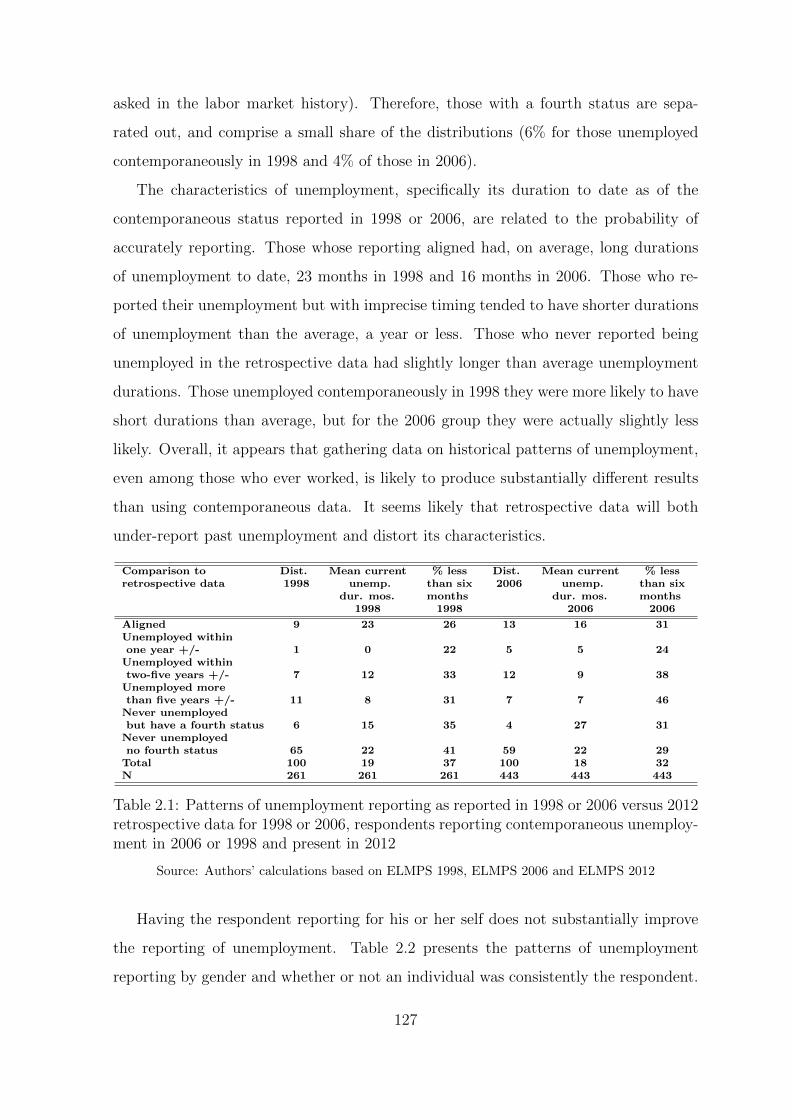
asked in the labor market history). Therefore, those with a fourth status are sepa-

rated out, and comprise a small share of the distributions (6% for those unemployed

contemporaneously in 1998 and 4% of those in 2006).

The characteristics of unemployment, specifically its duration to date as of the

contemporaneous status reported in 1998 or 2006, are related to the probability of

accurately reporting. Those whose reporting aligned had, on average, long durations

of unemployment to date, 23 months in 1998 and 16 months in 2006. Those who re-

ported their unemployment but with imprecise timing tended to have shorter durations

of unemployment than the average, a year or less. Those who never reported being

unemployed in the retrospective data had slightly longer than average unemployment

durations. Those unemployed contemporaneously in 1998 they were more likely to have

short durations than average, but for the 2006 group they were actually slightly less

likely. Overall, it appears that gathering data on historical patterns of unemployment,

even among those who ever worked, is likely to produce substantially different results

than using contemporaneous data. It seems likely that retrospective data will both

under-report past unemployment and distort its characteristics.

Comparison to Dist. Mean current % less Dist. Mean current % lessretrospective data 1998 unemp. than six 2006 unemp. than six

dur. mos. months dur. mos. months1998 1998 2006 2006

Aligned 9 23 26 13 16 31Unemployed withinone year +/- 1 0 22 5 5 24

Unemployed withintwo-five years +/- 7 12 33 12 9 38

Unemployed morethan five years +/- 11 8 31 7 7 46

Never unemployedbut have a fourth status 6 15 35 4 27 31

Never unemployedno fourth status 65 22 41 59 22 29

Total 100 19 37 100 18 32N 261 261 261 443 443 443

Table 2.1: Patterns of unemployment reporting as reported in 1998 or 2006 versus 2012retrospective data for 1998 or 2006, respondents reporting contemporaneous unemploy-ment in 2006 or 1998 and present in 2012

Source: Authors’ calculations based on ELMPS 1998, ELMPS 2006 and ELMPS 2012

Having the respondent reporting for his or her self does not substantially improve

the reporting of unemployment. Table 2.2 presents the patterns of unemployment

reporting by gender and whether or not an individual was consistently the respondent.

127

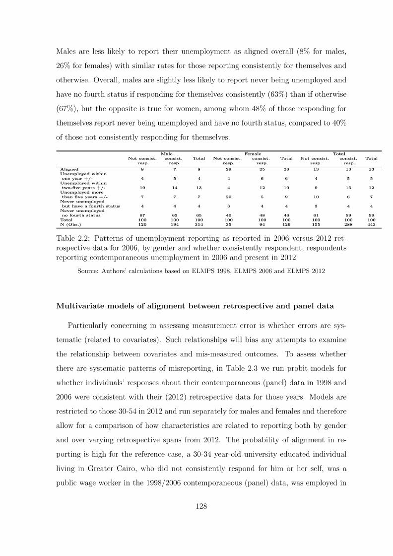
Males are less likely to report their unemployment as aligned overall (8% for males,

26% for females) with similar rates for those reporting consistently for themselves and

otherwise. Overall, males are slightly less likely to report never being unemployed and

have no fourth status if responding for themselves consistently (63%) than if otherwise

(67%), but the opposite is true for women, among whom 48% of those responding for

themselves report never being unemployed and have no fourth status, compared to 40%

of those not consistently responding for themselves.

Male Female TotalNot consist. consist. Total Not consist. consist. Total Not consist. consist. Total

resp. resp. resp. resp. resp. resp.

Aligned 8 7 8 29 25 26 13 13 13Unemployed withinone year +/- 4 5 4 4 6 6 4 5 5

Unemployed withintwo-five years +/- 10 14 13 4 12 10 9 13 12

Unemployed morethan five years +/- 7 7 7 20 5 9 10 6 7

Never unemployedbut have a fourth status 4 4 4 3 4 4 3 4 4

Never unemployedno fourth status 67 63 65 40 48 46 61 59 59

Total 100 100 100 100 100 100 100 100 100N (Obs.) 120 194 314 35 94 129 155 288 443

Table 2.2: Patterns of unemployment reporting as reported in 2006 versus 2012 ret-rospective data for 2006, by gender and whether consistently respondent, respondentsreporting contemporaneous unemployment in 2006 and present in 2012

Source: Authors’ calculations based on ELMPS 1998, ELMPS 2006 and ELMPS 2012

Multivariate models of alignment between retrospective and panel data

Particularly concerning in assessing measurement error is whether errors are sys-

tematic (related to covariates). Such relationships will bias any attempts to examine

the relationship between covariates and mis-measured outcomes. To assess whether

there are systematic patterns of misreporting, in Table 2.3 we run probit models for

whether individuals’ responses about their contemporaneous (panel) data in 1998 and

2006 were consistent with their (2012) retrospective data for those years. Models are

restricted to those 30-54 in 2012 and run separately for males and females and therefore

allow for a comparison of how characteristics are related to reporting both by gender

and over varying retrospective spans from 2012. The probability of alignment in re-

porting is high for the reference case, a 30-34 year-old university educated individual

living in Greater Cairo, who did not consistently respond for him or her self, was a

public wage worker in the 1998/2006 contemporaneous (panel) data, was employed in

128

2012, was a regular worker in 2012, and was a formal worker in 2012. For retrospec-

tive data referring to 1998, the reference case has a probability of alignment between

retrospective and panel data of more than 0.9. This is actually lower, around 0.8, for

retrospective data referring to 2006. Those 30-54 in 2012 would have been 24-48 in

2006 and 16-40 in 1998. Individuals may have an easier probability with retrospective

recall about first statuses than subsequent non-current statuses that causes the 1998

data, with more first statuses, to be more consistent. Compared to the university ed-

ucated, for males recalling distant (1998) statuses, all other education levels perform

significantly worse, but this pattern does not hold for females or males recalling less

distant (2006) statuses.

For males, compared to those 30-34 in 2012, those 35-44 in 2012, but not those

45-50 had significantly less alignment. For women there was at most a small increase

in consistency in reporting among older females (45-50) for more recent (2006) statuses.

Few regional differences occurred, with only slightly better alignment in Upper Egypt

for male’s more recent (2006) statuses. After controlling for other characteristics, there

were not significant differences in consistency dependent on whether or not the respon-

dent was consistently the individual in question. Where large differences did occur was

by both the retrospective status and 2012 employment characteristics. Compared to

public wage workers in the contemporaneous data (1998/2006), private wage workers

were significantly less likely to have consistent reports, non-wage workers even more so.

For men, those not working in the contemporaneous data were also significantly less

likely to report consistently, but there were no such differences for women. The magni-

tude of the differences is substantial; non-wage males had around a 30 percentage point

higher probability of disagreement, and non-wage women 66-72 percentage points. For

males, there are mixed differences comparing the effect sizes back to 2006 versus 2012.

For females, more recent reporting is consistently more aligned, although not by large

margins. In terms of 2012 employment characteristics, females not employed in 2012

are significantly more likely to consistently report their 1998 status, but not their 2006

status, while for males those not employed in 2012 are significantly less likely to re-

port their 2006 status but not their 1998 status. Both males and females who were

irregular in 2012 were significantly less likely to report their 2006 statuses consistently

129

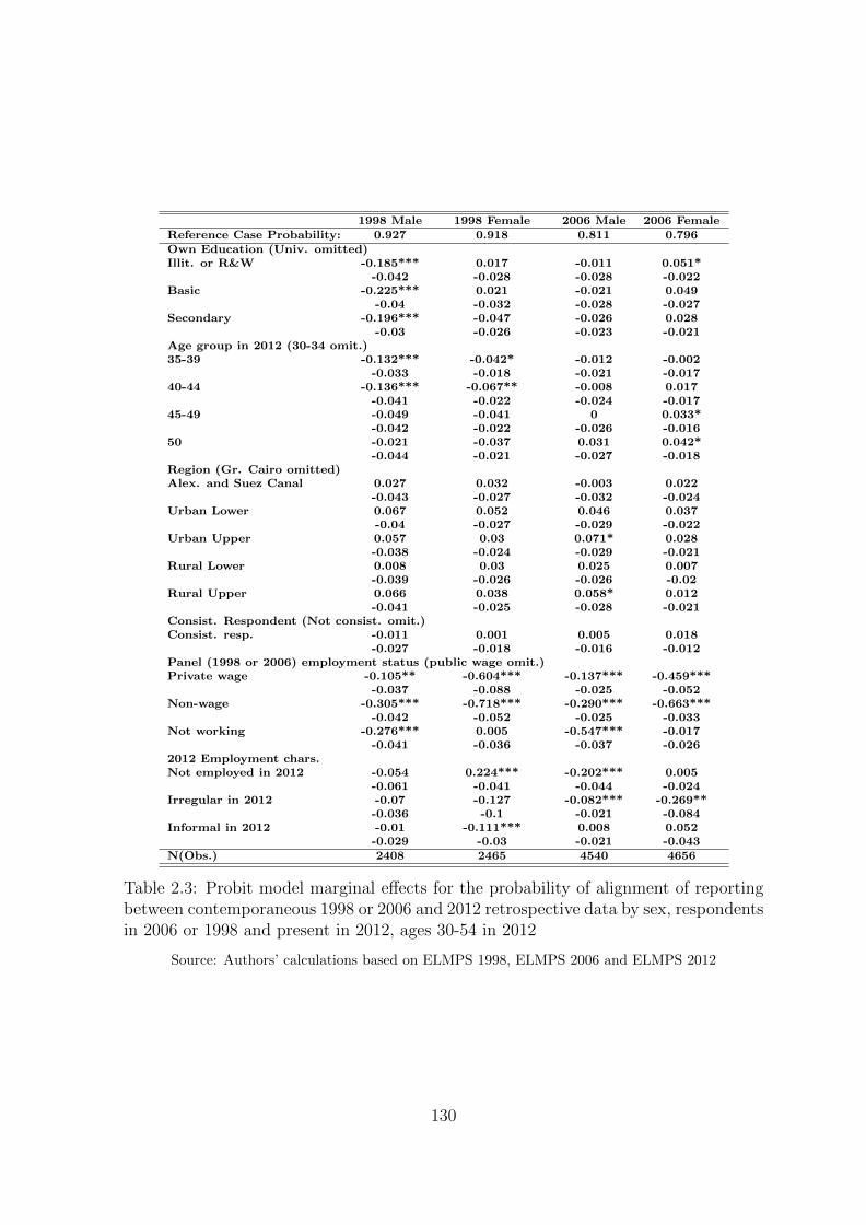
1998 Male 1998 Female 2006 Male 2006 FemaleReference Case Probability: 0.927 0.918 0.811 0.796Own Education (Univ. omitted)Illit. or R&W -0.185*** 0.017 -0.011 0.051*

-0.042 -0.028 -0.028 -0.022Basic -0.225*** 0.021 -0.021 0.049

-0.04 -0.032 -0.028 -0.027Secondary -0.196*** -0.047 -0.026 0.028

-0.03 -0.026 -0.023 -0.021Age group in 2012 (30-34 omit.)35-39 -0.132*** -0.042* -0.012 -0.002

-0.033 -0.018 -0.021 -0.01740-44 -0.136*** -0.067** -0.008 0.017

-0.041 -0.022 -0.024 -0.01745-49 -0.049 -0.041 0 0.033*

-0.042 -0.022 -0.026 -0.01650 -0.021 -0.037 0.031 0.042*

-0.044 -0.021 -0.027 -0.018Region (Gr. Cairo omitted)Alex. and Suez Canal 0.027 0.032 -0.003 0.022

-0.043 -0.027 -0.032 -0.024Urban Lower 0.067 0.052 0.046 0.037

-0.04 -0.027 -0.029 -0.022Urban Upper 0.057 0.03 0.071* 0.028

-0.038 -0.024 -0.029 -0.021Rural Lower 0.008 0.03 0.025 0.007

-0.039 -0.026 -0.026 -0.02Rural Upper 0.066 0.038 0.058* 0.012

-0.041 -0.025 -0.028 -0.021Consist. Respondent (Not consist. omit.)Consist. resp. -0.011 0.001 0.005 0.018

-0.027 -0.018 -0.016 -0.012Panel (1998 or 2006) employment status (public wage omit.)Private wage -0.105** -0.604*** -0.137*** -0.459***

-0.037 -0.088 -0.025 -0.052Non-wage -0.305*** -0.718*** -0.290*** -0.663***

-0.042 -0.052 -0.025 -0.033Not working -0.276*** 0.005 -0.547*** -0.017

-0.041 -0.036 -0.037 -0.0262012 Employment chars.Not employed in 2012 -0.054 0.224*** -0.202*** 0.005

-0.061 -0.041 -0.044 -0.024Irregular in 2012 -0.07 -0.127 -0.082*** -0.269**

-0.036 -0.1 -0.021 -0.084Informal in 2012 -0.01 -0.111*** 0.008 0.052

-0.029 -0.03 -0.021 -0.043N(Obs.) 2408 2465 4540 4656

Table 2.3: Probit model marginal effects for the probability of alignment of reportingbetween contemporaneous 1998 or 2006 and 2012 retrospective data by sex, respondentsin 2006 or 1998 and present in 2012, ages 30-54 in 2012

Source: Authors’ calculations based on ELMPS 1998, ELMPS 2006 and ELMPS 2012

130

but not their 1998 ones, possibly due to the rising volatility of their employment being

relatively recent (Assaad and Krafft, 2015c). Those males who were informal in 2012

were significantly less likely to report their 1998 status consistently. Overall, there are

mixed relationships between 2012 status and recall of past statuses, but definite dis-

agreements related to the contemporaneous (panel) employment type in the preceding

1998 or 2006 wave.

2.4.3 4.3 Comparing labor market transition rates across ret-

rospective versus panel data

An important application of retrospective and panel data on labor market statuses

is measuring transition rates between different labor market statuses in order to as-

sess labor market dynamics. We have demonstrated that there could be substantial

misalignment between contemporaneously measured statuses and ones measured by

means of retrospective questions, but also that the overall distribution of statuses is

fairly similar (Figure 2.7). If the measurement errors are primarily an issue of random

errors in the reporting of the timing of statuses, measures of labor market transition

rates could still be fairly sound. However, if entire statuses are lost (as appears to be

the case for unemployment), then measures of labor market dynamics will be under-

stated and will point to a more rigid labor market than is actually the case. Because

the ELMPS contains three panel waves, it is actually possible to assess labor market

transition rates by using either purely retrospective or purely panel data. This section

specifically compares transition rates, by status, from 1998 to 2006, based at first on

the 1998 and 2006 panel data, and second, on the retrospective data collected in 2012

for 1998 and 2006. This analysis is performed only for individuals who appear in all

three waves and who were 30-54 in 2012. The status used for classification purposes

comes from either the retrospective or the panel data, depending on which data are

being used to calculate the transition rates.

There are some key points to keep in mind when considering this comparison. The

contemporaneous status is (as is the case throughout this paper) the “usual” status in

the 3-month period preceding the survey, if an individual is employed. In the retrospec-

131

tive data coming from the labor market history module of the survey, statuses have to

be at least six months long to be reported. It is therefore likely that in the panel data

some of the transitions that are detected relate to statuses that lasted less than six

months and that would not be observed by definition in the retrospective data. This

would tend to inflate panel data transition rates upward, but probably not by much.

We know from the 2012 contemporaneous data that only 1.6% of employed individuals

have a different primary job in the reference week than in the reference three months,

suggesting that short-term transitions are rare. Transition rates in the panel data

are therefore only likely to be inflated by a few percentage points at most. Although

the probability of reporting statuses across panel and retrospective data is fairly sim-

ilar (Figure 2.7), the differences that do exist are going to affect the measurement of

transition rates as well.

In Figure 2.11, the rates of change in the various labor market statuses are assessed

using panel and retrospective data sources, according to the 1998 status. Notably, tran-

sition rates for males are under-stated by about half in the retrospective data relative to

the panel data (35% versus 59%) and by about two-thirds for females (9% versus 33%).

Looking across statuses, every employment status in 1998 suffers from under-reporting

problems, but to varying degrees. For males, transitions out of unemployment and

OLF statuses are fairly comparable, but this is not the case for females.

As well as differential rates of change, there are differential patterns of change in

terms of which transitions are detected or not detected (not shown). More subtle tran-

sitions, such as transitions from informal to formal private wage work or from employer

to self-employed and vice versa, are more likely to be missed in the retrospective data.

More distinctive transitions-such as those between public and private sector jobs and

between wage and non-wage work are also somewhat under-reported in the retrospec-

tive data, but to a lesser extent. Particularly for women, the retrospective data is less

able to detect transitions into and out of the out of the labor force. The problems

associated with detecting employment even contemporaneously among marginally em-

ployed women in agriculture and animal husbandry in Egypt are well known (Anker

(1995); Assaad (1997); Langsten and Salen (2008)). These problems are compounded

when the question refers to a reference period well in the past. Women in the public

132

Figure 2.11: Rates of status change in panel data for 1998 to 2006 versus rates of statuschange in retrospective data from 2012 for changes from 1998 to 2006 by sex and statusin 1998

Source: Authors’ calculations based on ELMPS 1998, ELMPS 2006 and ELMPS 2012 // Notes:Based only on individuals in all three waves. Status in 1998 is from either retrospective or panel datadepending on whether transition rates are being examined for retrospective or panel data. See Table2.20 for values underlying figure.

133

sector are much more likely to report being employed in the past. Since they typically

have low transition rates, this tends to understate overall transition rates for women.

2.4.4 Comparing the levels and trends of annualized labor

market transitions rates across two sets of retrospective

data from different waves of the survey

Measuring annualized transition rates from retrospective data

In order to further investigate the extent to which the ELMPS retrospective data

suffers from measurement problems, we compare the transition probabilities obtained

from the retrospective data for the same time period as assessed by different waves

of the survey. This analysis could serve as a guide for researchers wishing to use

similar surveys to generate annualized data from retrospective questions. Our overall

conclusion is that retrospective data tends to greatly understate the degree of dynamism

of the labor market and the longer the recall period, the greater the information loss.

The retrospective data from the ELMPS suffers from two major problems, the first

being the typical recall bias that attenuates the number of past transitions and the

second being the tendency of respondents to only recall past employment spells and

overlook non-employment spells. The latter problem may be an artifact of the confu-

sion on the part of interviewers and respondents between past labor market statuses

and past jobs. Accordingly, this section aims to deliver two key messages about the

retrospective data obtained from the ELMPS surveys. First, transition rates tend to be

underestimated when calculated using the annualized retrospective data. Second, the

time trends of these transitions are relatively reliable when analysing job-to-job flows,

especially if the time-series curves are smoothed. However, the trends for job/non-

employment flows are not well identified; these trends are distorted not only because of

recall errors but also due to the way the labor market history questions are interpreted

in the field. Throughout the restrospective accounts, non-employment spells are often

skipped, whether they are initial spells preceding first employment or interim spells

between two employment statuses.

To illustrate some of the challenges in working with retrospective data, we demon-

134

strate three different approaches to constructing retrospective data on the labor mar-

ket. Firstly, a naive basic panel of annualized labor market statuses is constructed

using only the retrospective chapter of the questionnaire. Respondents are therefore

limited to individuals who have ever worked and who report their past labor market

statuses. Second we augment this labor market history data with information about

recent unemployment spells from the current unemployment section of the question-

naire. We also incorporate information from the life events calendar on the timing of

non-employment spells of those who are currently out of the labor force. We refer to

this type of retrospective panel data as the “augmented panel”. Finally, we incorporate

information from those who have never worked, which should be considered in all anal-

yses of dynamics. By means of this analysis, we show that it would be quite misleading

to rely only on the labor market history information for those who have ever worked to

assess labor market dynamics. For these retrospective data to be useful, they must be

combined with the information on current unemployment for new entrants as well as

those who ever worked and with the longer employment history obtained from the life

events calendar. The dynamics we focus on are primarily the job finding (f) and sepa-

ration rates (s), which can be defined as the share of employed, E, and non-employed,

NE, changing states over time, t;

f =NEt−1 − EtNEt−1

(2.1)

s =Et−1 −NEt

Et−1

(2.2)

Separation rates

Turning first to the dynamics of separation rates, Figure 2.12 compares the differ-

ences across the three different annualized retrospective data construction approaches

using the 2012 retrospective data. The ELMPS 2012 questionnaire was redesigned to

ask about the past labor market statuses in a chronological order. Consequently, the

135

fourth status does not necessarily coincide with the current status for certain individ-

uals and moving from the labor market history data to the current state information

detects additional separations. Since separation rates are calculated relative to the

employed, adding in the never worked is irrelevant. The addition of the life events

calendar in the ELMPS 2012 might have also played a role, given that now individuals

who have gone recently out of the labor force have been captured, using the start date

of their inactivity status.

Although some dynamics are still mising in the new ELMPS 2012 design, as we

show below, the new structure of the retrospective questionnaire has generated smaller

bias in the dynamics obtained using the ELMPS 2012 than those obtained using the

ELMPS 2006 and the ELMPS 1998, especially when going back further in time. Yet a

subtantial amount of information about states individuals have occupied between the

fourth status of the labor market history and the current status is lost. According to

calculations from ELMPS 2012, about 34% of individuals who ever worked and had a

fourth status have exited that status. These two points indicate that while the new

design represents an improvement in the retrospective chapter in the questionnaire, the

addition of a fifth and sixth status to the labor market history section of the survey

might be valuable.

Figure 2.12: Comparing retrospective panels for employment to non-employment sep-aration rates, males 15-54 years of age, 1995-2011

Source: Authors’ calculations based on ELMPS 2012

136

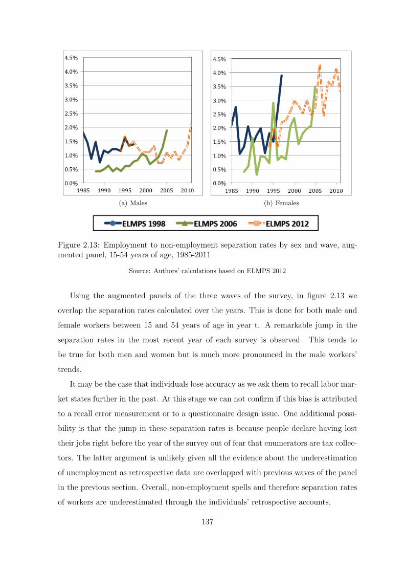
(a) Males (b) Females

Figure 2.13: Employment to non-employment separation rates by sex and wave, aug-mented panel, 15-54 years of age, 1985-2011

Source: Authors’ calculations based on ELMPS 2012

Using the augmented panels of the three waves of the survey, in figure 2.13 we

overlap the separation rates calculated over the years. This is done for both male and

female workers between 15 and 54 years of age in year t. A remarkable jump in the

separation rates in the most recent year of each survey is observed. This tends to

be true for both men and women but is much more pronounced in the male workers’

trends.

It may be the case that individuals lose accuracy as we ask them to recall labor mar-

ket states further in the past. At this stage we can not confirm if this bias is attributed

to a recall error measurement or to a questionnaire design issue. One additional possi-

bility is that the jump in these separation rates is because people declare having lost

their jobs right before the year of the survey out of fear that enumerators are tax collec-

tors. The latter argument is unlikely given all the evidence about the underestimation

of unemployment as retrospective data are overlapped with previous waves of the panel

in the previous section. Overall, non-employment spells and therefore separation rates

of workers are underestimated through the individuals’ retrospective accounts.

137

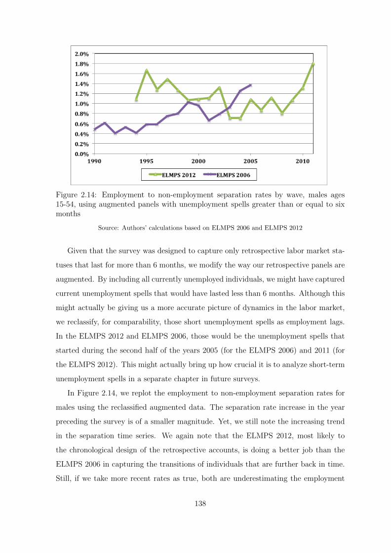
Figure 2.14: Employment to non-employment separation rates by wave, males ages15-54, using augmented panels with unemployment spells greater than or equal to sixmonths

Source: Authors’ calculations based on ELMPS 2006 and ELMPS 2012

Given that the survey was designed to capture only retrospective labor market sta-

tuses that last for more than 6 months, we modify the way our retrospective panels are

augmented. By including all currently unemployed individuals, we might have captured

current unemployment spells that would have lasted less than 6 months. Although this

might actually be giving us a more accurate picture of dynamics in the labor market,

we reclassify, for comparability, those short unemployment spells as employment lags.

In the ELMPS 2012 and ELMPS 2006, those would be the unemployment spells that

started during the second half of the years 2005 (for the ELMPS 2006) and 2011 (for

the ELMPS 2012). This might actually bring up how crucial it is to analyze short-term

unemployment spells in a separate chapter in future surveys.

In Figure 2.14, we replot the employment to non-employment separation rates for

males using the reclassified augmented data. The separation rate increase in the year

preceding the survey is of a smaller magnitude. Yet, we still note the increasing trend

in the separation time series. We again note that the ELMPS 2012, most likely to

the chronological design of the retrospective accounts, is doing a better job than the

ELMPS 2006 in capturing the transitions of individuals that are further back in time.

Still, if we take more recent rates as true, both are underestimating the employment

138

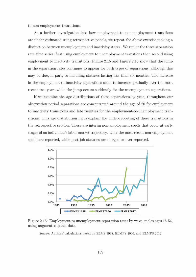
to non-employment transitions.

As a further investigation into how employment to non-employment transitions

are under-estimated using retrospective panels, we repeat the above exercise making a

distinction between unemployment and inactivity states. We replot the three separation

rate time series, first using employment to unemployment transtions then second using

employment to inactivity transitions. Figure 2.15 and Figure 2.16 show that the jump

in the separation rates continues to appear for both types of separations, although this

may be due, in part, to including statuses lasting less than six months. The increase

in the employment-to-inactivity separations seem to increase gradually over the most

recent two years while the jump occurs suddently for the unemployment separations.

If we examine the age distributions of these separations by year, throughout our

observation period separations are concentrated around the age of 20 for employment

to inactivity transitions and late twenties for the employment-to-unemployment tran-

sitions. This age distribution helps explain the under-reporting of these transitions in

the retrospective section. These are interim non-employment spells that occur at early

stages of an individual’s labor market trajectory. Only the most recent non-employment

spells are reported, while past job statuses are merged or over-reported.

Figure 2.15: Employment to unemployment separation rates by wave, males ages 15-54,using augmented panel data

Source: Authors’ calculations based on ELMS 1998, ELMPS 2006, and ELMPS 2012

139

Figure 2.16: Employment to inactivity separation rates for male workers between 15and 54 years of age

Source: Authors’ calculations based on ELMS 1998, ELMPS 2006, and ELMPS 2012

Apart from measurement error issues, the observed dynamics confirm the static

nature of the Egyptian labor market once an individual gets stabilized in a job. A lot

of churning occurs among the young, either between employment and unemployment

until they find what is probably a“suitable”job from their perspective, or either between

employment and inactivity, most likely for their military service. This explanation does

not mean however that if we exclude the young age group from our sample, we avoid

this separation uptick.

Job-finding rates

Moving now to the dynamics of the job finding process, recall that these rates are

the flow of workers from non-employment to employment relative to the stock of non-

employed. In this case, augmenting our retrospective panels, first with the currently

unemployed and then with the never worked does make a difference. Figure 2.17 shows

that adding information about current unemployment and inactivity spells is not trivial;

it gives a higher estimate of the stock of non-employed especially during the last two

to three years before the survey. These are most likely initial unemployment spells, i.e

people who have never had a job and consequently are not captured in the retrospective

140

part of the survey. Including everybody (ever and never work) in the analysis gives the

conceptually correct estimate of the stock of non-employed. Yet, it is only through the

current unemployment information that we can differentiate between unemployed and

inactive individuals with more than four statuses.

Figure 2.17: Comparing retrospective panels for non-employment to employment jobfinding rates by sex, ages 15-54, 1995-2011

Source: Authors’ calculations based on ELMS 1998, ELMPS 2006, and ELMPS 2012

As was true for the job finding rates time series, we again suspect an underesti-

mation of the non-employed as we go back in time. This time, the job-finding rates

calculated from our retrospective panels are over-estimated. The most reliable point,

in terms of the level of the job-finding rate, is likely to be the most recent point. Figure

2.18 shows the overlap of the the three finding rates time series calculated from the

three retrospective panels using augmented data and incorporating those who never

worked. We note likely over-estimation in the job finding rates mirroring the likely

under-estimation we noted above in the separation rates. If we set aside the levels

issue, and focus of the trend of both finding and separation rates over time, we note

that there has been a very slight increase in the job finding rates over time for males

and almost no substantial chnge for the females. A relatively higher increase in the

separation rates over time is observed for both male and female workers.

141

Figure 2.18: Non-employment to employment job finding rates by sex and wave, ages15-54, using augmented panel data and incorporating those who never worked

Source: Authors’ calculations based on ELMS 1998, ELMPS 2006, and ELMPS 2012

Job-to-job transitions

Having examined states and transitions between employment and non-employment,

we now examine job-to-job transitions among the employed. The comparisons of retro-

spective and panel data showed that more aggregated employment statuses are likely to

be more consistently reported. For instance, it appears that respondents have difficulty

distinguishing between informal and formal employment states as well as regular and

irregular work. Therefore, we limit the analysis of the retrospective transitions rates

to three broad employment sectors, namely public wage work, private wage work and

non-wage work.

In Figure 2.19, we overlap the job-to-job transition rates calculated using the

ELMPS 2006 and ELMPS 2012 retrospective panels. These rates are obtained by

dividing the number of workers transitioning from one sector to another between years

t and t+1 by the number of workers employed in the origin sector in year t. Generally,

we observe a close overlap of the job-to-job transition rates obtained using the two

different retrospective panel data sets. This finding suggests that using retrospective

accounts give consistent conclusions about the trends of job-to-job transition rates over

time, especially when these trends are smoothed. However, it’s crucial to note that the

142

(a) Public to Private wage work (b) Public to Non-wage work

(c) Private to Public wage work (d) Private to Non-wage work

(e) Non-wage to Public wage work (f) Non-wage to Private wage work

Figure 2.19: Job-to-job transitions by wave, male workers, ages 15-54 calculated fromretrospective panels

Source: Authors’ calculations based on ELMPS 2006 and ELMPS 2012

143

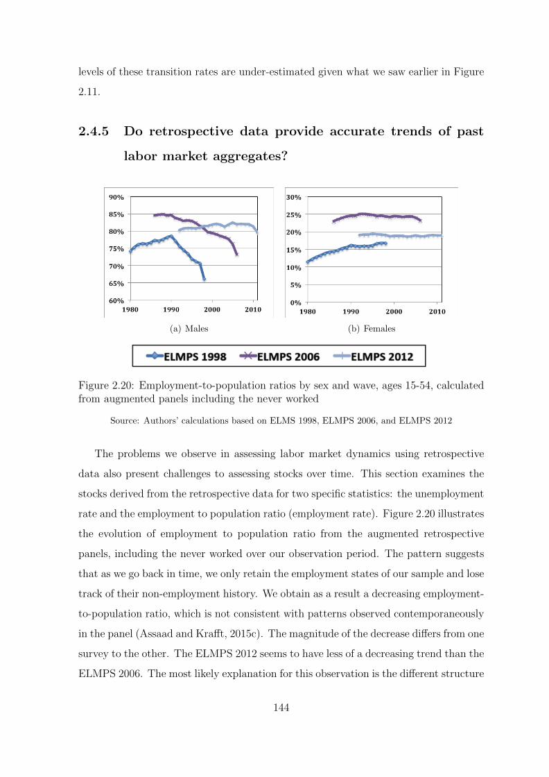
levels of these transition rates are under-estimated given what we saw earlier in Figure

2.11.

2.4.5 Do retrospective data provide accurate trends of past

labor market aggregates?

(a) Males (b) Females

Figure 2.20: Employment-to-population ratios by sex and wave, ages 15-54, calculatedfrom augmented panels including the never worked

Source: Authors’ calculations based on ELMS 1998, ELMPS 2006, and ELMPS 2012

The problems we observe in assessing labor market dynamics using retrospective

data also present challenges to assessing stocks over time. This section examines the

stocks derived from the retrospective data for two specific statistics: the unemployment

rate and the employment to population ratio (employment rate). Figure 2.20 illustrates

the evolution of employment to population ratio from the augmented retrospective

panels, including the never worked over our observation period. The pattern suggests

that as we go back in time, we only retain the employment states of our sample and lose

track of their non-employment history. We obtain as a result a decreasing employment-

to-population ratio, which is not consistent with patterns observed contemporaneously

in the panel (Assaad and Krafft, 2015c). The magnitude of the decrease differs from one

survey to the other. The ELMPS 2012 seems to have less of a decreasing trend than the

ELMPS 2006. The most likely explanation for this observation is the different structure

144

Figure 2.21: Unemployment rates, males, ages 15-64, calculated from augmented ret-rospective panels including the never worked compared to those reported in the LFSS

Source: Authors’ calculations based on ELMS 1998, ELMPS 2006, ELMPS 2012, and LFSS data(based on CAPMAS’s bulletin of the Labor Force Sample Survey for 1989-2011)

of the ELMPS 2012 questionnaire. Asking individuals about their past statuses in a

chronological order, starting with the first status, rather than backward in time as

was the case in 1998 and 2006, may have increased consistency of employment trends.

However, none of these approaches recovers the pattern of employment observed in the

panel contemporaneous statuses, which is an increase in employment rates over time

for men and a rise and fall in employment rates for women.

Superimposing the retrospective data and the unemployment rates from the official

Labor Force Sample Survey (LFSS) further illustrates how the proportions of different

labor market states and consequently labor market transitions get distorted if one uses

retrospective data. Figure 2.21 shows that the retrospective data does not align with

the evolution of Egypt’s unemployment rate over the past two decades as reported in

official statistics.

2.5 Conclusion

The primary objective of this paper is to assess whether it is possible to collect

information about labor market dynamics using retrospective data or if recall error is so

great as to make panel data the only viable option. As expected, we conclude that it is

possible to garner useful information on labor market dynamics from retrospective data,

145

but one must be cautious about which information to trust and at what level of detail.

One of our most basic conclusions is that information on past employment collected

using retrospective data can be fairly reliable, so long as fine distinctions between

employment states are not made. For instance, the distinctions between employer

and self-employed, between formal and informal wage work, or regular and irregular

wage work are not easily made using retrospective data. The regularity of work is

something that can change frequently depending on the state of labor demand in the

economy and should therefore not be a subject of retrospective questions. Even the

distinction between self-employment and irregular wage work is sometimes difficult to

make especially for men engaged in small-scale agriculture. Smallholders often do not

have enough land to keep them fully occupied on their small farms and must often

engage in multiple livelihood strategies that may either involve non-agricultural self-

employment or irregular wage work.

In the case of women engaged in self-employment, whether in agriculture or outside

agriculture, the distinction between being employed and not employed is hard enough

to make in contemporaneous data, let alone in retrospective data. In Egypt, women

in this kind of employment typically do not consider themselves to be employed and

may move frequently between employment and non-employment states, as defined by

international labor statisticians. To assess their current status accurately, researchers

must use complex keyword-based questions that inquire about a large number of ac-

tivities, and even this detailed approach often fails to elicit reliable estimates of female

participation in home-based self-employment and unpaid family labor (Anker (1995);

Assaad and El-Hamidi (2009); Assaad (1997); Langsten and Salen (2008)). It is im-

possible to ask questions at this level of detail about a retrospective period, casting

doubt on the employment transitions obtained from retrospective data for women in

self-employment. Conversely, transitions across well-defined employment states, such

as between public and private wage work, or between public wage work and non-wage

work can be captured fairly reliably using retrospective data. Spells of non-employment

interspersed between employment spells are usually hard to recall, whether they are

unemployment spells or spells outside the labor force altogether. For instance, 71% of

those observed as unemployed in the 1998 wave and 64% of the unemployed in 2006

146

wave of the survey never reported any unemployment at any time in the past in the

retrospective data obtained from them in the 2012 wave. Thus transitions from non-

employment to employment and vice-versa will be understated in retrospective data,

with important implications for the accurate reporting of separation rates for the em-

ployed and job-finding rates for either the unemployed or those outside the labor force,

and the stock of unemployed in past dates. Generally, these rates will be understated,

and possibly increasingly so as we go back in time, confounding any measurement

of trends. In contrast, trends describing job-to-job transitions can be captured more

reliably using retrospective data.

Another conclusion we derived from analyzing the reporting of recalled marriage

costs is that retrospective questions eliciting monetary amounts are unreliable at best.

Even when asked to report the nominal amount paid at the time, at least some respon-

dents tend to inflate the amount to their equivalent value at the time of the survey.

It thus becomes impossible to ascertain monetary trends over time when some of the

data is inflated and some of it is not.

This research has also produced valuable lessons about how to use existing ret-

rospective data from the ELMPS or other similar surveys. It is tempting to create

annualized retrospective panel data from the labor market history module of the ques-

tionnaire and use those to calculate various transition rates. However, the labor market

history module of the questionnaire is only applicable to people who have ever worked,

excluding people at risk of transitioning to employment who may not have ever worked.

Moreover, because of the limitations on the number of states that the questionnaire

inquires about (up to four), the retrospective data may not reach up to the current

state. To correct for the possible biases than can result from this, the labor market

history data must be augmented by information from the current employment or un-

employment sections of the questionnaire and from the life events calendar, which can

potentially include more transitions to and from employment. Finally, it needs to be

augmented by adding individuals who have never worked but who are currently either

unemployed or out of the labor force. In adding data from the current section of the

survey, it is important to correct for the fact that current spells may last for less than

six months and may therefore not be comparable to spells captured in the retrospective

147

data. Individuals currently unemployed for less than six months should potentially be

reclassified to their previous status to ensure compatibility of definitions.

Finally, this experience has allowed us to derive some important lessons on how

to improve questionnaire design to collect more accurate retrospective data. First, in

comparing the retrospective data from 2012 to the data from previous rounds, we de-

termined it is preferable to ask questions about the individual’s labor market trajectory

in chronological rather than in reverse chronological order. It elicits better informa-

tion about labor market insertion and in particular about any initial unemployment

spells prior to first employment. Second, we suspect that many respondents (and pos-

sibly interviewers) interpreted status to mean job, contributing to the underreporting

of non-employment spells. It is probably a good idea to explicitly ask about whether

there was an initial non-employment or unemployment spell prior to the first job and to

explicitly ask whether the end of each job was followed by a period of non-employment

that exceeded a six-month duration. Third, it is necessary to ask those who have never

worked and are currently inactive about whether they have ever sought employment

and about the timing and length of the spell in which they were seeking employment,

at least for the first time. Fourth, although the addition of a life events calendar that

elicits information about the start and end dates of all employment states helps fill some

of the gaps, it may still be valuable to elicit information in the labor market history

module about a fifth and possibly sixth labor market state to capture the transitions

of individuals with more numerous transitions.

Given budgetary and availability constraints, the retrospective panels are currently

the only available panels in the MENA region that allow researchers study labor mar-

ket dynamics, particularly short-term transitions or flows. Having discussed the errors

encountered in retrospective data, it is important to note however that it is possible

to use some remedies that attenuate these measurement errors and eventually pro-

duce unbiased (or possibly less biased) results. A possible solution would be to match

biased moments obtained from retrospective data with reliable accurate moments ob-

tained from auxiliary contemporaneous cross-sectional data. Of course, this could be

obtained from the same dataset or an external data source, so long comparability be-

tween the data sets is verified. In this case, one assumes that the information obtained

148

from the contemporaneous data is the most accurate. Assumptions about the (func-

tional) form of the “forgetting rate” or information loss in the retrospective data would

also be required. Langot and Yassine (2015) (chapter 3) correct the ELMPS aggre-

gate labor market transition rates between employment, unemployment and inactivity

states, obtained from the retrospective panels, using this methodology. They assume

that the most recent year of the latter panels are the most accurate and that people

report more distant events less accurately. The measurement error has a functional

form that increases exponentially as one goes back in time. This methodology can al-

low the re-construction of corrected separation and job finding time series that can be

used in the analysis of the macroeconomic trends of the labor market. This can even be

extended to make use of the micro-level information available about the labor market

transitions. Using the aggregate measurement errors estimated for the different types

of transitions, one could distribute these errors in the form of weights to the individuals

in the survey (Yassine (no date), chapter 5). Again, assumptions need to be made on

how to attribute weights to the individuals. Yassine (no date) (chapter 5) discusses two

ways of doing so: (1) a naive method: where all individuals are assumed to be corrected

similarly i.e. proportional weights and (2) a differentiated method: where weights are

predicted based on the probability an individual would make a certain type of transi-

tion. All the above assumed that the information in retrospective panels is correct, just

a little bit over reported or under-reported with respect to the true contemporaneous

points (i.e. true moments). Another possible solution, with a different assumption,

would be to estimate the alignment rate, possibly the rate of telling the truth, and

eventually creating a weight such that individuals who report the truth have higher

weights. This requires however the availability of both micro-level contemporaneous

and retrospective information for the same individuals. In our case, it could be applied

to the ELMPS but not to other datasets, for instance the Jordan Labor Market Panel

Survey (JLMPS) and the Tunisia Labor Market Panel Survey, where only one wave is

available. Drawbacks of how representative the sample becomes after the creation of

such weights need to be also discussed.

One possible solution to the missing non-employment states problem would be

stressing on the targeted meaning of retrospective statuses in the training of the enu-

149

merators. Additionally, we suggest adding questions about the end dates of each status

throughout the retrospective section rather than relying on the start date of the next

status. Even if people interpret the retrospective state as a job status, this additional

information could help to capture the interim non-employment state, which starts at

the end date of the prior job and ends at the start date of the next job.

To conclude, we believe that panel data with short retrospective modules to fill in the

gaps between waves of the panel are the best data we can hope for, short of continuous

administrative data, to study labor market dynamics. However, in the absence of such

panel data, useful information can be obtained from retrospective questions, so long as

some of the lessons we draw here are kept in mind.

150

References

Anker, R. (1995): “Measuring Female Labour Force with Emphasis on Egypt Richard

Anker and Martha Anker,” Gender and Development in the Arab World: Women’s

Economic Participation: Patterns and Policies, p. 148.

Artola, C., and U.-L. Bell (2001): “Identifying labour market dynamics using

labour force survey data,” .

Assaad, R. (1997): “The employment crisis in Egypt: Current trends and future

prospects,” Research in Middle East Economics, 2(1), 39–66.

Assaad, R., and F. El-Hamidi (2009): “Women in the Egyptian labor market:

an analysis of developments, 1988-2006,” The Egyptian Labor Market Revisited, pp.

259–284.

Assaad, R., and C. Krafft (2013): “The Egypt labor market panel survey: intro-

ducing the 2012 round,” IZA Journal of Labor & Development, 2(1), 1–30.

(2014): “Youth Transitions in Egypt: School, Work, and Family Formation

in an Era of Changing Opportunities,” Discussion Paper 14-1, Silatech.

(2015a): “The Economics of Marriage in North Africa: A Unifying Theoret-

ical Framework,” in The Oxford Handbook of Africa and Economics: Contexts and

Concepts (Vol. 1), pp. 72–85. Oxford University Press.

(2015b): “An Empirical Analysis of the Economics of Marriage in Egypt,

Morocco, and Tunisia,” in The Oxford Handbook of Africa and Economics: Contexts

and Concepts (Vol. 2), pp. 533–555. Oxford University Press.

151

(2015c): “The Structure and Evolution of Employment in Egypt: 1998-2012,”

in The Egyptian Labor Market in an Era of Revolution, pp. 27–51. Oxford University

Press.

Assaad, R., C. Krafft, and C. Yassine (2015): “Comparing Retrospective and

Panel Data Collection Methods to Assess Labor Market Dynamics,” Discussion pa-

per, Economic Research Forum, Cairo.

Assaad, R., and M. Ramadan (2008): “Did housing policy reforms curb the delay in

marriage among young men in Egypt?,” Middle East Youth Initiative Policy Outlook,

1, 1–8.

Assaad, R., and R. Roushdy (2009): “An analysis of sample attrition in the Egypt

Labor Market Panel Survey 2006,” The Egyptian labor market revisited, pp. 303–315.

Beckett, M., J. Da Vanzo, N. Sastry, C. Panis, and C. Peterson (2001):

“The quality of retrospective data: An examination of long-term recall in a developing

country,” Journal of Human Resources, pp. 593–625.

Beegle, K., C. Carletto, and K. Himelein (2012): “Reliability of recall in agri-

cultural data,” Journal of Development Economics, 98(1), 34–41.

Beegle, K., J. De Weerdt, J. Friedman, and J. Gibson (2012): “Methods of

household consumption measurement through surveys: Experimental results from

Tanzania,” Journal of Development Economics, 98(1), 3–18.

Black, D. A., M. C. Berger, and F. A. Scott (2000): “Bounding parameter

estimates with nonclassical measurement error,” Journal of the American Statistical

Association, 95(451), 739–748.

Blossfeld, H.-P., K. Golsch, and G. Rohwer (2012): Event history analysis

with Stata. Psychology Press.

Bound, J., C. Brown, and N. Mathiowetz (2001): “Measurement error in survey

data,” Handbook of econometrics, 5, 3705–3843.

152

Carroll, R. J., D. Ruppert, L. A. Stefanski, and C. M. Crainiceanu (2006):

Measurement error in nonlinear models: a modern perspective. CRC press.

De Nicola, F., and X. Gine (2014): “How accurate are recall data? Evidence from

coastal India,” Journal of Development Economics, 106, 52–65.

Dercon, S., and J. S. Shapiro (2007): “Moving On, Staying Behind, Getting Lost:

Lessons on poverty mobility from longitudinal data.,” .

Dhillon, N., P. Dyer, and T. Yousef (2009): “Generation in Waiting: An

Overview of School to Work and Family Formation Transitions,” Generation in Wait-

ing: The Unfulfilled Promise of Young People in the Middle East, pp. 11–38.

Finn, A., and V. Ranchhod (2013): Genuine Fakes: The prevalence and implica-

tions of fieldworker fraud in a large South African survey. Southern Africa Labour

and Development Research Unit.

Fuller, W. A. (2009): Measurement error models, vol. 305. John Wiley & Sons.

Gibson, J., and B. Kim (2010): “Non-Classical Measurement Error in Long-Term

Retrospective Recall Surveys,” Oxford Bulletin of Economics and Statistics, 72(5),

687–695.

Grosh, M., and P. Glewwe (2000): Designing Household Survey Questionnaires for

Developing Countries: Lessons from 15 Years of the Living Standards Measurement

Study, Volume 2. Washington, DC: World Bank.

Heitjan, D. F., and D. B. Rubin (1990): “Inference from coarse data via multiple

imputation with application to age heaping,” Journal of the American Statistical

Association, 85(410), 304–314.

Hiroyuki, N., S. Yasuyuki, and T. Mari (2010): “Asking Retrospective Questions

in Household Surveys: Evidence from Vietnam,” Discussion paper.

Judge, G., and L. Schechter (2009): “Detecting problems in survey data using

Benford’s Law,” Journal of Human Resources, 44(1), 1–24.

153

Kherfi, S. (2015): “Determinants of Unemployment Duration in Egypt,” in The Egyp-

tian Labor Market in an Era of Revolution, pp. 90–107. Oxford University Press.

Langot, F., and C. Yassine (2015): “Reforming employment protection in Egypt:

An evaluation based on transition models with measurement errors,” Discussion pa-

per, Economic Research Forum, Cairo.

Langsten, R., and R. Salen (2008): “Two approaches to measuring women’s work

in developing countries: A comparison of survey data from Egypt,” Population and

Development Review, 34(2), 283–305.

Magnac, T., and M. Visser (1999): “Transition models with measurement errors,”

Review of Economics and Statistics, 81(3), 466–474.

Puetz, D., J. Von Braun, and D. Puetz (1993): “Improving data quality in house-

hold surveys,” Data Needs for Food Policy in Developing Countries: New Directions

for Household Surveys.

Roberts, J. M., and D. D. Brewer (2001): “Measures and tests of heaping in

discrete quantitative distributions,” Journal of Applied Statistics, 28(7), 887–896.

Salem, R. (2012): “Trends and Differentials in Jordanian Marriage Behavior: Mar-

riage Timing, Spousal Characteristics, Household Structure, and Matrimonial Ex-

penditures,” .

(2015): “Changes in the Institution of Marriage in Egypt from 1998 to 2012,” in

The Egyptian Labor Market in an Era of Revolution, pp. 162–181. Oxford University

Press.

(no date): “Imagined Crises: Assessing Evidence of Delayed Marriage and

Never-Marriage in Contemporary Egypt,” in Domestic Tensions, National Anxieties:

Global Perspectives on Marriage Crisis. Oxford University Press.

Singerman, D. (2007): “The economic imperatives of marriage: Emerging practices

and identities among youth in the Middle East,” Middle East Youth Initiative Work-

ing Paper, (6).

154

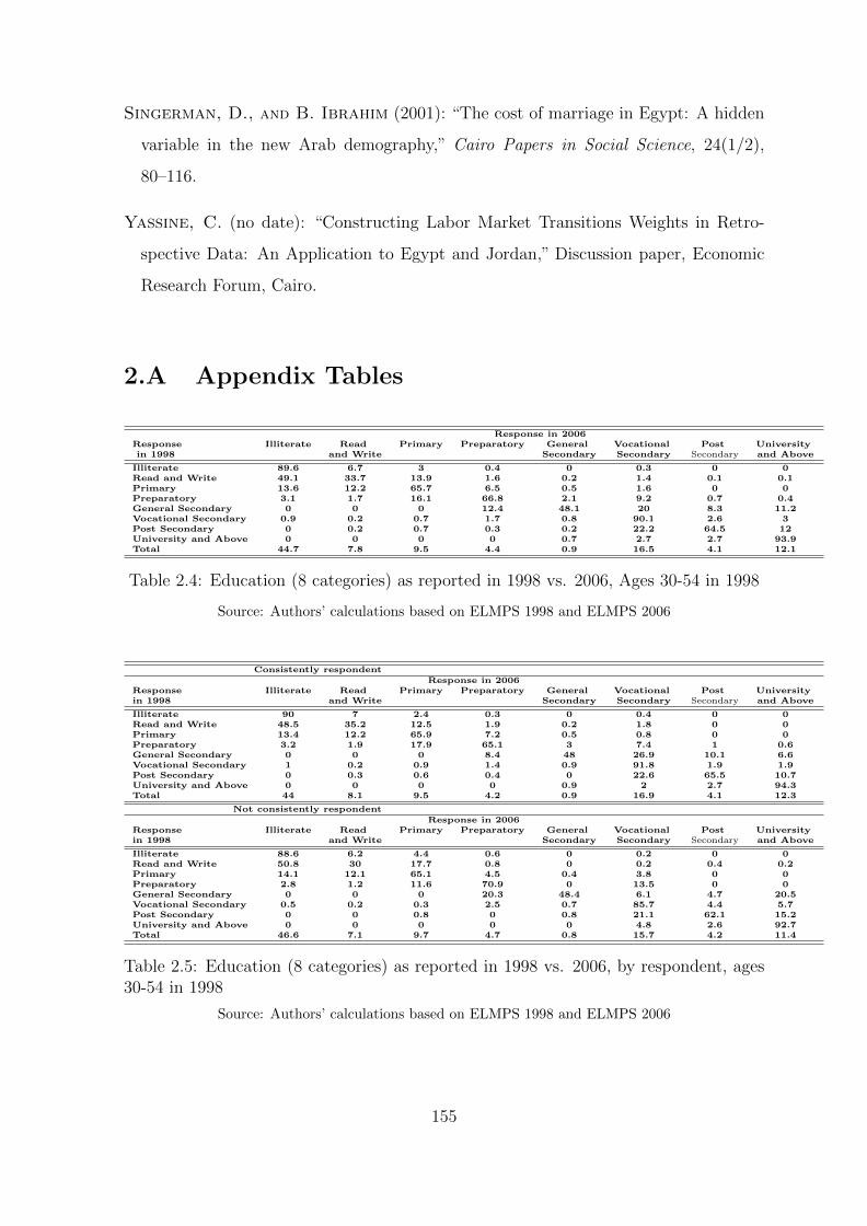
Singerman, D., and B. Ibrahim (2001): “The cost of marriage in Egypt: A hidden

variable in the new Arab demography,” Cairo Papers in Social Science, 24(1/2),

80–116.

Yassine, C. (no date): “Constructing Labor Market Transitions Weights in Retro-

spective Data: An Application to Egypt and Jordan,” Discussion paper, Economic

Research Forum, Cairo.

2.A Appendix Tables

Response in 2006Response Illiterate Read Primary Preparatory General Vocational Post Universityin 1998 and Write Secondary Secondary Secondary and Above

Illiterate 89.6 6.7 3 0.4 0 0.3 0 0Read and Write 49.1 33.7 13.9 1.6 0.2 1.4 0.1 0.1Primary 13.6 12.2 65.7 6.5 0.5 1.6 0 0Preparatory 3.1 1.7 16.1 66.8 2.1 9.2 0.7 0.4General Secondary 0 0 0 12.4 48.1 20 8.3 11.2Vocational Secondary 0.9 0.2 0.7 1.7 0.8 90.1 2.6 3Post Secondary 0 0.2 0.7 0.3 0.2 22.2 64.5 12University and Above 0 0 0 0 0.7 2.7 2.7 93.9Total 44.7 7.8 9.5 4.4 0.9 16.5 4.1 12.1

Table 2.4: Education (8 categories) as reported in 1998 vs. 2006, Ages 30-54 in 1998

Source: Authors’ calculations based on ELMPS 1998 and ELMPS 2006

Consistently respondentResponse in 2006

Response Illiterate Read Primary Preparatory General Vocational Post Universityin 1998 and Write Secondary Secondary Secondary and Above

Illiterate 90 7 2.4 0.3 0 0.4 0 0Read and Write 48.5 35.2 12.5 1.9 0.2 1.8 0 0Primary 13.4 12.2 65.9 7.2 0.5 0.8 0 0Preparatory 3.2 1.9 17.9 65.1 3 7.4 1 0.6General Secondary 0 0 0 8.4 48 26.9 10.1 6.6Vocational Secondary 1 0.2 0.9 1.4 0.9 91.8 1.9 1.9Post Secondary 0 0.3 0.6 0.4 0 22.6 65.5 10.7University and Above 0 0 0 0 0.9 2 2.7 94.3Total 44 8.1 9.5 4.2 0.9 16.9 4.1 12.3

Not consistently respondentResponse in 2006

Response Illiterate Read Primary Preparatory General Vocational Post Universityin 1998 and Write Secondary Secondary Secondary and Above

Illiterate 88.6 6.2 4.4 0.6 0 0.2 0 0Read and Write 50.8 30 17.7 0.8 0 0.2 0.4 0.2Primary 14.1 12.1 65.1 4.5 0.4 3.8 0 0Preparatory 2.8 1.2 11.6 70.9 0 13.5 0 0General Secondary 0 0 0 20.3 48.4 6.1 4.7 20.5Vocational Secondary 0.5 0.2 0.3 2.5 0.7 85.7 4.4 5.7Post Secondary 0 0 0.8 0 0.8 21.1 62.1 15.2University and Above 0 0 0 0 0 4.8 2.6 92.7Total 46.6 7.1 9.7 4.7 0.8 15.7 4.2 11.4

Table 2.5: Education (8 categories) as reported in 1998 vs. 2006, by respondent, ages30-54 in 1998

Source: Authors’ calculations based on ELMPS 1998 and ELMPS 2006

155

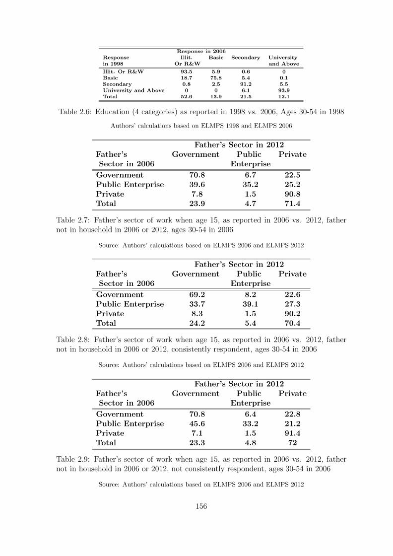
Response in 2006Response Illit. Basic Secondary Universityin 1998 Or R&W and Above

Illit. Or R&W 93.5 5.9 0.6 0Basic 18.7 75.8 5.4 0.1Secondary 0.8 2.5 91.2 5.5University and Above 0 0 6.1 93.9Total 52.6 13.9 21.5 12.1

Table 2.6: Education (4 categories) as reported in 1998 vs. 2006, Ages 30-54 in 1998

Authors’ calculations based on ELMPS 1998 and ELMPS 2006

Father’s Sector in 2012Father’s Government Public PrivateSector in 2006 Enterprise

Government 70.8 6.7 22.5Public Enterprise 39.6 35.2 25.2Private 7.8 1.5 90.8Total 23.9 4.7 71.4

Table 2.7: Father’s sector of work when age 15, as reported in 2006 vs. 2012, fathernot in household in 2006 or 2012, ages 30-54 in 2006

Source: Authors’ calculations based on ELMPS 2006 and ELMPS 2012

Father’s Sector in 2012Father’s Government Public PrivateSector in 2006 Enterprise

Government 69.2 8.2 22.6Public Enterprise 33.7 39.1 27.3Private 8.3 1.5 90.2Total 24.2 5.4 70.4

Table 2.8: Father’s sector of work when age 15, as reported in 2006 vs. 2012, fathernot in household in 2006 or 2012, consistently respondent, ages 30-54 in 2006

Source: Authors’ calculations based on ELMPS 2006 and ELMPS 2012

Father’s Sector in 2012Father’s Government Public PrivateSector in 2006 Enterprise

Government 70.8 6.4 22.8Public Enterprise 45.6 33.2 21.2Private 7.1 1.5 91.4Total 23.3 4.8 72

Table 2.9: Father’s sector of work when age 15, as reported in 2006 vs. 2012, fathernot in household in 2006 or 2012, not consistently respondent, ages 30-54 in 2006

Source: Authors’ calculations based on ELMPS 2006 and ELMPS 2012

156

2006 2006 retro. 1998 1998 retro.contemp. from 2012 contemp. from 2012

Public 27.9 29.9 20.7 21.5Private formal regular wage workers 12.3 11 5.3 7.5Private informal regular wage workers 16.3 16 10.5 13.6Irregular wage workers 8.9 16.3 14.2 16.8Employers 14.1 11.1 7.3 6.4Self-Employed 9.5 9.7 5.2 6.4Unpaid Family Work 5 2.6 6.5 5.1Unemployed 2.8 0.9 7.3 2.3OLF 3.4 2.7 23.1 20.3Total 100 100 100 100

Table 2.10: Labor Market Status, as reported contemporaneously for 1998 and 2006and as reported retrospectively for those years from 2012 data, male respondents ages30-54 in 2012 present in both waves

Source: Authors’ calculations based on ELMS 1998, ELMPS 2006 and ELMPS 2012

2006 2006 retro. 1998 1998 retro.contemp. from 2012 contemp. from 2012

Public 12.9 13.4 10.6 11.3Private formal regular wage workers 1.1 1.2 0.7 0.5Private informal regular wage workers 1.3 1.7 1.3 1.4Irregular wage workers 0.6 0.9 0.8 0.8Employers 1 0.7 0.3 0.3Self-Employed 4 1.9 1.9 1.5Unpaid Family Work 10 4.4 5.5 2.8Unemployed 4.5 1.5 6.6 1.4OLF 64.5 74.3 72.3 80Total 100 100 100 100

Table 2.11: Labor Market Status, as reported contemporaneously for 1998 and 2006and as reported retrospectively for those years from 2012 data, female respondents ages30-54 in 2012 present in both waves

Source: Authors’ calculations based on ELMS 1998, ELMPS 2006 and ELMPS 2012

Public Private Private Irregular Employers Self-Employed Unpaid Unemployed OLFformal informal wage Familyregular regular worker Workwage wage

Public 87.6 4.3 2.6 1.6 1.3 1.3 0.2 0.3 0.8

Private formalregular wage 14.8 43.6 20.4 10.8 3.2 4.9 0.6 1.2 0.5

Private informalregular wage 7 14 32.8 24.6 7.7 8.1 1.9 1.2 2.7

Irregularwage worker 6.6 4.6 19.8 45.7 8.3 10.8 2.3 1 1.1

Employers 5 2.9 13.8 17.7 39.8 15.3 4.2 0.2 1.2

Self-Employed 3.6 4.9 13.2 20.4 16.9 36.7 1.7 0.4 2.1

UnpaidFamily Work 4.6 5.3 23.6 19.7 16.8 8.7 19.4 0.9 1

Unemployed 13.7 14.9 27.1 16.8 1.8 5.4 5.7 5.1 9.5

OLF 7.9 6.9 15.2 16.8 6.6 7.2 1.7 3.4 34.3

Total 29.9 11 16 16.3 11.1 9.7 2.6 0.9 2.7

Table 2.12: Labor Market Status, as reported in 2006 versus 2012 retrospective datafor 2006, male respondents ages 30-54 in 2012 present in both waves

Source: Authors’ calculations based on ELMPS 2006 and ELMPS 2012

157

Public Private Private Irregular Employers Self-Employed Unpaid Unemployed OLFformal informal wage Familyregular regular worker Workwage wage

Public 85 4.2 2.6 4 1.4 0.4 0.4 1.1 1

Private formalregular wage 9.7 47.8 19 10.8 1.2 4.8 2.5 0.2 3.9

Private informalregular wage 5.6 10.2 34 21.1 8.6 6 1.1 3.5 10

Irregularwage worker 5.5 5.4 19.4 38.1 8.2 8.7 5.7 1.2 7.8

Employers 3.6 7.3 15 17.4 28.3 17.3 9.3 0.4 1.4

Self-Employed 7.8 2.2 13.5 21.4 11.8 25 10.9 0.2 7.1

UnpaidFamily Work 2.2 0.9 13.4 21.9 10.8 6.4 19.6 5.1 19.6

Unemployed 3.9 12 15.1 26.4 3.5 6.5 4.9 6.3 21.5

OLF 4.2 3.1 8.7 9.1 1.4 3.2 4.5 3.1 62.7

Total 21.5 7.5 13.6 16.8 6.4 6.4 5.1 2.3 20.3

Table 2.13: Labor Market Status, as reported in 1998 versus 2012 retrospective datafor 1998, male respondents ages 30-54 in 2012 present in both waves

Source: Authors’ calculations based on ELMPS 1998 and ELMPS 2012

Public Private Private Irregular Employers Self-Employed Unpaid Unemployed OLFformal informal wage Familyregular regular worker Workwage wage

Public 88.7 2.6 0.6 0 0 0.3 0 1.1 6.8

Private formalregular wage 18.1 32.7 17.3 0 0 0 0 2.1 29.9

Private informalregular wage 4.4 7.8 26.5 3 1.2 4 0 8.2 45

Irregularwage worker 0 0 8.5 34.5 0 11.2 7.1 1.9 36.8

Employers 0.9 0 3.3 0 17.7 14 9.7 0 54.4

Self-Employed 0.9 0 2.2 1.3 3.9 17.7 8.1 0.3 65.7

UnpaidFamily Work 1.2 0 0 0.5 1.6 3.3 20.2 1.2 72

Unemployed 4.9 3.1 4.8 0 0 0.7 1.8 5.5 79.2

OLF 2 0.4 1.1 0.8 0.2 0.9 2.9 1.3 90.4

Total 13.4 1.2 1.7 0.9 0.7 1.9 4.4 1.5 74.3

Table 2.14: Labor Market Status, as reported in or 2006 versus 2012 retrospective datafor 2006, female respondents ages 30-54 in 2012 present in both waves

Source: Authors’ calculations based on ELMPS 2006 and ELMPS 2012

158

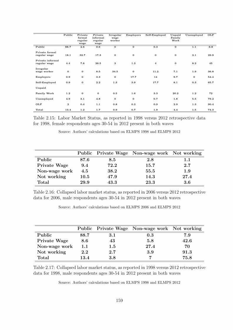
Public Private Private Irregular Employers Self-Employed Unpaid Unemployed OLFformal informal wage Familyregular regular worker Workwage wage

Public 88.7 2.6 0.6 0 0 0.3 0 1.1 6.8

Private formalregular wage 18.1 32.7 17.3 0 0 0 0 2.1 29.9

Private informalregular wage 4.4 7.8 26.5 3 1.2 4 0 8.2 45

Irregularwage worker 0 0 8.5 34.5 0 11.2 7.1 1.9 36.8

Employers 0.9 0 3.3 0 17.7 14 9.7 0 54.4

Self-Employed 0.9 0 2.2 1.3 3.9 17.7 8.1 0.3 65.7

Unpaid

Family Work 1.2 0 0 0.5 1.6 3.3 20.2 1.2 72

Unemployed 4.9 3.1 4.8 0 0 0.7 1.8 5.5 79.2

OLF 2 0.4 1.1 0.8 0.2 0.9 2.9 1.3 90.4

Total 13.4 1.2 1.7 0.9 0.7 1.9 4.4 1.5 74.3

Table 2.15: Labor Market Status, as reported in 1998 versus 2012 retrospective datafor 1998, female respondents ages 30-54 in 2012 present in both waves

Source: Authors’ calculations based on ELMPS 1998 and ELMPS 2012

Public Private Wage Non-wage work Not working

Public 87.6 8.5 2.8 1.1Private Wage 9.4 72.2 15.7 2.7Non-wage work 4.5 38.2 55.5 1.9Not working 10.5 47.9 14.3 27.4Total 29.9 43.3 23.3 3.6

Table 2.16: Collapsed labor market status, as reported in 2006 versus 2012 retrospectivedata for 2006, male respondents ages 30-54 in 2012 present in both waves

Source: Authors’ calculations based on ELMPS 2006 and ELMPS 2012

Public Private Wage Non-wage work Not working

Public 88.7 3.1 0.3 7.9Private Wage 8.6 43 5.8 42.6Non-wage work 1.1 1.5 27.4 70Not working 2.2 2.7 3.9 91.3Total 13.4 3.8 7 75.8

Table 2.17: Collapsed labor market status, as reported in 1998 versus 2012 retrospectivedata for 1998, male respondents ages 30-54 in 2012 present in both waves

Source: Authors’ calculations based on ELMPS 1998 and ELMPS 2012

159

Public Private Wage Non-wage work Not working

Public 85 10.7 2.3 2Private Wage 6.3 66.3 17.7 9.7Non-wage work 4.3 37.8 46.8 11.2Not working 4.1 28.8 10.5 56.7Total 21.5 38 17.8 22.6

Table 2.18: Collapsed labor market status, as reported in 2006 versus 2012 retrospectivedata for 2006, female respondents ages 30-54 in 2012 present in both waves

Source: Authors’ calculations based on ELMPS 2006 and ELMPS 2012

Public Private Wage Non-wage work Not working

Public 86.7 1.6 0 11.7Private Wage 9.4 24.2 9.9 56.6Non-wage work 1.2 3.2 12.8 82.9Not working 2.2 2 4.3 91.5Total 11.3 2.7 4.6 81.4

Table 2.19: Collapsed labor market status, as reported in 1998 versus 2012 retrospectivedata for 1998, female respondents ages 30-54 in 2012 present in both wave

Source: Authors’ calculations based on ELMPS 1998 and ELMPS 2012

Male FemaleRetrospective Panel Retrospective Panel

Public 2 11 6 11Private formal regular wage workers 21 45 20 55Private informal regular wage workers 27 63 41 82Irregular wage workers 25 73 49 95Employers 7 43 0 68Self-Employed 15 61 17 69Unpaid Family Work 66 74 11 77Unemployed 97 90 56 85OLF 88 89 8 25Total 35 59 9 33

Table 2.20: Rates of status change in panel data for 1998 to 2006 versus rates of statuschange in retrospective data from 2012 for changes from 1998 to 2006 by sex and statusin 1998

Authors’ calculations based on ELMPS 1998, ELMPS 2006 and ELMPS 2012

160

Part II

The Impact of Labor Market

Policies and Institutions on Labor

Market Outcomes

161

Chapter 3

Reforming Employment Protection

in Egypt: An Evaluation Based on

Transition Models with

Measurement Errors 1

3.1 Introduction

The history of institutions in most developing countries led their labor markets to be

very rigid, where private sector contractual opportunities approached the rules of public

sector appointments. Major international organizations have therefore encouraged re-

forms, to introduce more flexibility in these labor markets. The importance of ensuring

a healthy dynamic labor market lies in creating more productive jobs and destroying

less productive ones (see Veganzones-Varoudakis and Pissarides (2007)). Increased dy-

namics also scales down the difference between formal employment and informal work,

which is very flexible by definition. By attracting more workers to formal jobs, the

1This chapter is based on work conducted jointly with Francois Langot. This work has benefitedfrom a financial grant from the Economic Research Forum. The contents and recommendations donot necessarily reflect the views of the Economic Research Forum. We thank R. Assaad, D. Margolis,F. Fontaine and J. Wahba for helpful comments as well as seminar participants at University ofParis 1 Pantheon-Sorbonne, Paris School of Economics (SIMA-Maison des Sciences Economique) andUniversity of Maine (GAINS-TEPP). Participants at the Economic Research Forum workshop“Impactof Labor Market Regulations and Institutions on Labor Market Performance and Outcomes”and WorldBank conference on“Markets, Labor and Regulations”also provided valuable remarks and suggestions.

162

shift of employment into the formal sector allows an increase in the fiscal revenues of

governments and hence reduces their budgetary deficits.

The importance of a more flexible labor market was recognized by the Egyptian

Government in 2003, as they introduced the new labor law (No.12). The new Egypt

labor law came to action in 2004 aiming at increasing the flexibility of the hiring and

firing processes in Egypt. The law provides comprehensive guidelines for recruitment,

hiring, compensation and termination of employees. It directly addresses the right

of the employer to terminate an employee’s contract and the conditions in which it

performs under.

Although flexible employment protection strategies have been recommended, eco-

nomic theory predicts ambiguous effects of increased flexibility on the performance

of labor markets. Indeed, when the policy change is perfectly anticipated, the conven-

tional model of Mortensen and Pissarides (1994) shows that facilitating the termination

of employees leads to increased job finding rates, but also has a direct positive effect

on transitions from employment to unemployment. Since the employment rate is an

increasing function of job finding rates but a decreasing function of separations, eval-

uating a policy that increases labor market flexibility necessitates the analysis of the

different elasticities of these two rates of transitions to the reform in question. Even if

the policy change is unexpected, given that the hirings and separations are jump vari-

ables, the same reasoning applies. Even if the effects on unemployment are ambiguous,

the liberalization of the labor market promotes new job and hence high productivity.

It hence becomes crucial to assess the adjustment of the Egyptian overall separation

and job finding rates (the two main components of Egypt’s unemployment rate) to such

a more flexible employment protection strategy, introduced by the new 2003 labor law.

In general, only one earlier study by Wahba (2009) investigated the short term impact

(i.e after two years) of the law but on the formalization process in Egypt. Our paper

is able to reply to the following research questions:

1. Investigate the evolution of worker flows trend over the period 1998-2012, and

link changes in the job finding and separation rates to the New Egyptian Labor

Law implemented in 2004.

163

2. Build up a model in a way that enables us to simulate labor market policies and

examine their implications on dynamics of the Egyptian labor market.2

From a methodological point of view, the construction of the observed labor market

transitions from microeconomic data, as developed by Shimer (2005, 2012), seems to

be a perfect fit to assess this type of labor market reforms. It’s a methodology that

allows to exploit rich labor market surveys, to disentangle the changes in all transitions

and to deduce using a simple balance of flows, the impact on aggregates, such as the

rate of unemployment. In this paper, we try to use this construction methodology, to

create aggregate flows from microeconomic surveys in the spirit of the work of Shimer.

From an econometric point of view, the reform will be analyzed as a break in the series

of job finding and separation rates. The aggregated effect on unemployment will be

deduced from the composition of the differentiated effects of transition rates.

The originality of our work lies in the construction of the flow dynamics time series

of the Egyptian labor market. As in most countries in the project development process,

micro surveys which trace the history of each individual every month are unavailable.

Only a labor market panel survey where individuals report their retrospective and cur-

rent accounts of their labor market states is repeated almost every 6 years. Even with

high quality collection methods and accurate cross-validated questions, such surveys

and retrospective information are subject to a memory bias (recall error).3 De Nicola

and Gine (2014) have shown that the magnitude of the recall error increases over time,

in part because respondents resort to inference rather than memory. Their findings

are based on a comparison between administrative records and retrospective survey

data from a developing country, more precisely a sample of self-employed households

engaged in fishing in costal India. Using data of a developed country (USA), Poterba

and Summers (1986) find through audits of employment surveys that correcting em-

ployment self-reports can change the estimated duration of unemployment by a factor

of two. Thus, the methodological contribution of our paper is to propose an original

2This can be made without any problem concerning the Lucas (1976) criticisim because separationand job finding rates are jump variables, and given that the policy change is unexpected.

3Given the long time interval between the waves of the survey, we can not use simple methodsof memory bias correction used in annual surveys to reconstruct monthly data from retrospectivecalendars. See e.g. Hairault, Le Barbanchon, and Sopraseuth (2013) for such methods applied onFrench data.

164

method correcting this recall error, using the markovian structure of the labor market

transitions. We structurally estimate using Simulated Method of Moments (SMM) a

function representing the ”forgetting rate” conditional on the individual’s state in the

labor market. Our model is close to the one developed by Magnac and Visser (1999).

Given the importance of taking into consideration the entry and exit of the labor force,

in an attempt to portray the Egyptian labor market as fully as possible, and to test

the robustness of our method, we extend our analysis to a three-state model of the

labor market (employment, unemployment and inactivity) and check if the results on

unemployment rates, reconstructed from a series of corrected labor market flows, are

consistent. We show that estimates of corrections then yield similar results, suggest-

ing that our statistical correction method produces robust series. Consequently, we can

conclude that our method can be applied to multiple surveys only available between two

relatively spaced dates (points in time), which is often the case in developing countries.

The paper uses the Egypt labor market panel surveys (ELMPS 2006 and ELMPS

2012) to extract annual and semi-annual synthetic retrospective panel data sets over

the period 1999-2012. As mentioned above, given the nature of our data (with a wave

repeated almost every 6 years), we were concerned with recall error. We were also

concerned by a potential design bias in our data due to the very rich information

obtained about the most recent employment/non-employment vector versus relatively

limited information about past trajectories. We hence develop our novel methodology

to correct for the “recall and design” error in the labor market transitions time series.

In his 2012 article, Shimer shows that reconstructing workers flows from microeco-

nomic surveys gives the advantage to job finding rates in explaining fluctuations of the

US unemployment. His results therefore contrast with those obtained by Blanchard

and Diamond (1990) and Davis and Haltiwanger (1990, 1992): these authors showed

that, based on statistics of job creations and destructions (job flows), the majority of

fluctuations in the US unemployment rate arise from the job destruction rate. In our

article, despite the use of a methodology similar to that proposed by Shimer (2012),

we show that the new 2003 labor law had significant positive effects on the separation

rates, but barely any on the job finding rates. The increase in separation rates therefore

outweighs the no significant change in job finding rates leading to an increase in the

165

unemployment rates after the reform. These results are valid whether we include or

exclude the inactivity state from our analysis. By performing counterfactuals analysis,

we show evidence of the increasing dominant role of the separation rates in account-

ing for Egyptian unemployment fluctuations. It’s important to note however that the

separation and job finding rates remain at extremely low levels reflecting a very rigid

nature of the Egyptian labor market.

These empirical results can be viewed as inconsistent with the usual Mortensen and

Pissarides (1994) model, where an increase in the labor market flexibility (modeled

as a downward shift of the firing costs) would definitely increase the separation and

the finding rates. Indeed, such a policy which reduces tax distortions should lead

as well to increasing the match surplus (even if the job duration will be reduced),

and consequently the job finding rate. At this point, it becomes therefore difficult to

explain the no change in job finding rates even though there has been a decrease in

the firing costs using the conventional Mortensen and Pissarides (1994) model. It’s

true one can explain this by the time lag between the employers reaction to the reform

between separating more workers directly after the implementation of the policy and

hiring more workers only when they feel confident enough about the market. However,

among the possible explanations behind such an observed unusual phenomenon could

be the fact that Egypt is a developing country where corruption is one of the main

barriers to business encountered by the entrepreneurs. We show theoretically how the

Mortensen and Pissarides (1994) can account for this phenomenon and hence to match

our data.4

The rest of the paper is divided as follows. The second section surveys the literature

and exposes the value added by our paper. Section 3 briefly presents the data used

in our analysis, the creation of the synthetic retrospective panel data sets and the

potential error treatments. Section 4 discusses the presence of recall and design bias

4Another way to explain this puzzle is to extend the Mortensen and Pissarides (1994) to accountfor the informal and public sectors, which represent big shares of employment. Even though the policyis directed to the formal private sector, it surely affects the interaction and the flow of workers betweenthe different employment sectors. The conventional aggregate Mortensen and Pissarides (1994) modelfails to explain the inside story of these inter-sectoral transitions. Langot and Yassine (2015) (chapter4) attempt to extend the Mortensen and Pissarides (1994) to model the different transitions betweenthe formal, informal and public sectors and hence try to explain the possible reasons behind onlyseparations increasing in response to a more flexible labor market.

166

in our transition matrices and hence a model is built and estimated to correct for the

bias. Section 5 explores the econometric methodology adopted. Section 6 presents our

estimation methodology and results. Section 7 provides counterfactual experiments and

policy implications. Section 8 surveys the (Mortensen and Pissarides, 1994) theoretical

model and shows how it fails to explain our empirical results, except if we introduce

corruption. We then finally conclude.

3.2 Value Added and Literature Survey

Egypt has long been ranked as a country with very rigid labor laws (see WorldBank

(2014)). This has stemmed from the time when virtually all industrial employment was

public sector and heavily unionized. In 1990, the private sector accounted at most for

23 percent of Egypt’s manufacturing sector output, and 25 percent of its employees.

Very bureaucratic rules were established. Fear of social costs of privatization may

have kept these rules rigid, especially the costs of paying off fired workers.5 Different

labor regulations indices have unsurprisingly shown that Egypt, was ranked one of the

most rigid among the MENA region countries, which are themselves the most restrictive

developing countries, after the Latin American region (see (Veganzones-Varoudakis and

Pissarides, 2007) and (Campos and Nugent, 2012))6. This index decreases substantially

to reach a level lower than 1.5 during the period 2000-2004 after a long period of

stagnation around a level of 1.8 for about three decades since 1970. Indeed, the Law 12

of the New 2003 Labor Code seems to have relatively reduced the state’s role, giving

greater leeway to employers to hire and fire.7 With such a reform, should an employer

need to go out of business, he gets the right to lay off all workers. In case of economic

necessity, an employer has the right to lay off workers or modify contracts given that he

5The crisis of the beginning of the 90’s, compelled the government to look to the InternationalMonetary Fund (IMF), World Bank and the Paris Club for support, where Egypt was required toundergo a structural adjustment package as a counterpart to receiving a stand-by credit. The resultwas an increase in economic activity, and strong growth in private-sector manufacturing. By 2003,the share of the Egyptian total industrial value added reached 70 percent and employment increasedsubstantially to 60 percent.

6Veganzones-Varoudakis and Pissarides (2007) underline the ranking of the different developingcountry regions from the least to the most rigid as follows: South Asia (1.25), Sub-Saharan Africa(1.45), East Asia (1.6), MENA (1.65), Latin America (2.05), with the index of labor market regulationbetween parenthesis.

7The new 2003 law also gives greater leeway to employers to set wages and benefits.

167

provides a notice period of 2 months for an employee of less than 10 years seniority, and

3 months if seniority is over 10 years. Severance payments of an amount of 1 month

per year for workers with less than 5 years experience and of an amount of 1.5 months

per year after that are implemented (see WorldBank (2014) for more details).

Unfortunately , the impact of the new 2003 labor market reform has been rarely as-

sessed. It’s extremely important to measure whether the policy has achieved its direct

objective on the labor market’s flexibility in general, the separation and finding rates in

particular, as well as it’s consequent effect on the national unemployment. Policy eval-

uation techniques necessitate the availability of time series labor market flows to detect

structural changes in a given labor market. In a country like Egypt where available

data and analyses are hinged on static, cross-sectional and aggregate approaches, our

mission becomes difficult. The limitations and potential errors synthetic panel data,

constructed from retrospective accounts, are subject to, prevents research from con-

firming trends and results obtained by simple descriptive statistics8. Previous research

as a result hardly satisfied the urge to explore the true story of the dynamics of the

Egyptian Labor market and the effect of reforms on the labor market outcomes. This

paper therefore aims at enriching the existing literature and exploring the effect of the

new labor law implemented in 2004 on separation and job finding rates, about which we

know very little from the official aggregate data and statistics (as has been explained

in chapters 1 and 2).

The paper also overcomes the budget constraints limiting annual data collection

to follow workers through their careers by benefiting from the existing two waves of

the Egypt Labor Market Panel Survey (2006 and 2012) as well as by the improved

techniques we adopt to construct trajectory panels for individuals within these surveys

from the retrospective accounts to provide us with annual panel data sets. Our tech-

niques don’t limit to only capturing these trajectories and labor market dynamics but

8See Assaad, Krafft, and Yassine (2015) (chapter 2) for detailed evidence on how different labormarket statuses, especially unemployment, are prone to misreporting over time, comparing retrospec-tive and contemporaneous data for the same individuals over time using the Egypt Labor MarketPanel Surveys 1998, 2006 and 2012.

168

also to correcting the recall and design9 bias from which our retrospective data tend

to suffer.10 Like previous research, as for example De Nicola and Gine (2014), we were

concerned by the recall bias observed in our retrospective calendars. Uncorrected pre-

liminary descriptives might give false impressions about the dynamics of worker flows

and unemployment in Egypt. In the literature on measurement error in transition

models, two approaches are used. The first approach, in the tradition of the semi-

nal papers of Poterba and Summers (1986, 1995), uses either validation or reinterview

data (assuming that these data is error free) to estimate the measurement error. While

Poterba and Summers (1986) use the reinterview data from the Current Population

Survey to study the impact of measurement error on the estimated number of labor

market transitions, Magnac and Visser (1999) use prospective and retrospective data

for the same time period to study labor mobility of French workers with the Labor

Force Survey, where the prospective data was being treated as error-free. The second

approach, used for example by Rendtel, Langeheine, and Berntsen (1998), is applied

when no auxiliary (error-free) information is available. Based on the assumption of

the Independent Classification Errors11, these methods use latent Markov model with

measurement error. In Magnac and Visser (1999) and Bassi, Hagenaars, Croon, and

Vermunt (2000), this method is extended to the case where correlation between errors

are possible, also by using retrospective data.

Nevertheless, these methods are designed for short term analysis of the labor market

(the impact of the business cycle on labor market transitions). They use surveys where

annual waves are available, and which include intra-annual information. In this per-

spective, the measurement error can be approximated as a small noise, with an update

9Recall bias is defined as respondents mis-reporting their retrospective trajectory because theytend to forget some events or spells, especially the short ones. The design bias arises from thefact that different types of questions are being asked for current versus recall/retrospective statuses.There is therefore a question of salience/cognitive recognition by the respondents where by asking thequestions differently, respondents, or even sometimes the enumerators themselves, can interpret themdifferently. Yassine (2014) (chapter 1) and Assaad, Krafft, and Yassine (2015) (chapter 2) show forinstance that due to the questionnaire design of the ELMPS, statuses in the retrospective sections arebeing interpreted more of job statuses rather than labor market states.

10In an investigation of the effect of measurement error on poverty transitions in the German Socio-Economic Panel (GSOEP), Rendtel, Langeheine, and Berntsen (1998) conclude that approximatelyhalf of the observed transitions are due to measurement error. Lollivier and Daniel (2002) corroboratethis result for the European Community Household Panel (ECHP).

11This assumption means that the errors made at two subsequent time periods are conditionallyindependent given the true states

169

each year at the time of the interview. In our case, the delay between the two interviews

is much longer, requiring a new method to correct for long-term memory recall bias. In

addition to the recall bias, we also suspect a potential design bias in our constructed

synthetic panel data sets, due to differences in the nature of questions asked about the

current or most recent labor market status and those asked about the individuals’ his-

tories. We therefore add to the existing literature by applying a new theoretical model

to correct for the bias observed in our data, for both a two-state and a multiple state

labor market. Empirically, the technique we use to extract a retrospective panel and

correct for “recall and design” bias using the Egyptian Labor market data sets would

definitely allow researchers and policy-makers (who use the same or similar data sets)

to use these data sets for further research and needed investigations about labor market

dynamics. We also use the cross-sectional information obtained from a third wave of

the Egypt Labor Market Panel Survey in 1998, to verify the results we obtain using our

corrected transition rates time series. We explain in the data section the limitations of

this data set and why we choose not to use it in our econometric estimations.

3.3 Data and Sample Selection

Our paper relies on the Egypt Labor Market Panel Surveys 1998, 2006 and 2012,

the first, second and third rounds of a periodic longitudinal survey that tracks the labor

market and demographic characteristics of households and individuals interviewed in

1998. The households selected in the longitudinal data are national-representative and

randomly selected. The final sample interviewed in 2012 consists of 12060 households,

which includes 6752 original households (out of 8371 interviewed in 2006, which followed

itself 4816 households interviewed in 1998), 3308 split households and a refresher sample

of 2000 households. The attrition cross-sectional and panel weights attributed in these

data sets by Assaad and Krafft (2013) allow to expand sample figures to a macro

population level.

We make use in this paper of the rich retrospective information available in both

questionnaires as well as current state information and the newly added chapter (in

ELMPS12) of life events’ calendar. Unfortunately, the ELMPS 1998 round did not

170

contain what we require as “full” (compared to ELMPS06 and ELMPS12) retrospective

accounts about the interviewed individuals. The type and different characteristics of an

individual’s first state in the labor market have not been collected. We therefore choose

to only use the cross-section stocks from this round in our analysis, for identification

and comparability reasons in the correction model, given that it does not contain the

minimal information required to extract the longitudinal retrospective panel data.

Following the methodology adopted by Yassine (2014) (chapter 1), we extract two

retrospective panel datasets for the periods 1999-2006 (from ELMPS06) and 1999-2012

(from ELMPS12). ELMPS06 records only the year of start of an individuals’ state

allowing us to just extract an annual panel data set between 1999-2006. The availability

of the month and year of the date of start of a state in ELMPS12, on the other

hand, enables the extraction of both semi-annual and annual transitions. Since missing

values about the month and year of start of a state are problematic when creating such

synthetic panels, we adopted the same assumptions made in Yassine (2014) (chapter

1) to create the ELMPS12 panel datasets. Consequently, the cross-state transitions do

not get evenly distributed over the 2 semesters of the year. Semi-annual transitions are

not representative for a 6 months period. However as they are lumped into an annual

trajectory, this allows us to capture the maximum range of transitions an individual

went through during the year t. Cross-state labor market transitions such as job finding

and job separations are therefore derived from the semi-annual constructed panel, but

then lumped into annual transitions in order to be representative as well as comparable

with the 1999-2006 panel extracted from the ELMPS0612.

The general sample of the retrospective panel datasets includes individuals who

answered the retrospective question i.e those who ever worked in the Egyptian labor

market, the young unexperienced new entrants and the individuals who are perma-

nently out of the labor force.

In this paper, we focus on employed, unemployed and inactive male individuals

between 15 and 49 years of age. Our analysis exclude female workers since their move-

ment in and out of the labor market most of the time follow personal motives such

as marriage and child birth. Moreover, going back in time, our sample should have

12See Yassine (2014) (chapter 1) for a detailed discussion of this procedure.

171

included people who were alive back then but passed away by the year of the survey

i.e. 2006 and 2012 and hence did not respond to the ELMPS questionnaire. Due to

this backward attrition, we were obliged to limit the age of our analysis group to what

we refer to as the prime age group (i.e. between 15 and 49 years old). Another reason

why one would want to avoid including old people within our analysis group is to limit

recall error which is intuitively likely to increase with advanced age.

A potential type of error that our data is susceptible to face is the response error

including the “present” mis-report bias and recall bias (Yassine, 2014). We cannot deal

with the bias resulting from people deliberately mis-reporting their present employment

status and information to avoid taxes and government registers. We therefore assume

the non-existence of this bias. The extent of recall bias is examined and corrected by

our constructed model in the next section.

In addition to the recall error, we also suspect the presence of what we call the “de-

sign”bias that leads to a systematic inaccuracy (in the same direction of the recall bias)

in our constructed synthetic panels. The ELMPS survey contains very detailed (almost

complete) questions about an individual’s current employment/unemployment/inactivity

state. Questions about retrospective accounts are however minimal and very broad,

where people mostly end up recording their jobs history ignoring histories about their

unemployment spells. It’s also worth noting that individuals responding to the retro-

spective chapter in the survey are required to to have at least one work experience.

Consequently, using the available collected data, we obtain correct estimate for current

labor market state and increasingly biased estimates as we move backwards, especially

among the unemployed and inactive who have never worked before. We examine in the

next section the nature of the bias observed in the data and suggest a methodology to

correct for it.

Finally, it’s important to note that in this paper we have two stages of analysis;

one where an individual can occupy one of two states, namely employment (E) or

unemployment (U). The transition from employment to unemployment is referred to

as job separation and the transition from unemployment to employment is referred to

as job finding. A three-state (Employment [E] - Unemployment [U] - Inactivity [I])

model is also developed where all inter- and intra- state transitions are illustrated and

172

are used to calculate the job finding and separation rates of the three-state economy

following Shimer (2012).

3.4 Recall and Design Bias

We first describe the link between worker flows and stocks data. Secondly, we

present our method that corrects the data from the ”recall and design bias”. In the last

part of this section, we present our “corrected” data.

3.4.1 Descriptive Statistics

Following Diamond-Mortensen-Pissarides (DMP) matching model of unemployment,

in steady-state equilibrium, flows into unemployment (“separations”) equal flows from

unemployment (“finds”). Using the flow balance equation, we therefore have

fU︸︷︷︸Probability to find a job × no. of unemployed

= sE︸︷︷︸Probability to quit/lose a job × no. of employed

(3.1)

We can therefore show that in equilibrium, unemployment rate is

U

L︸︷︷︸Unemployment Rate

=s

s+ f(3.2)

This represents the rate of unemployment to which the economy naturally gravitates

in the long run. The natural rate of unemployment is determined by looking at the rate

people are finding jobs, compared with the rate of job separation (i.e. People quitting

either voluntarily or involuntarily in our case), and not the size of the population or

the economy. In any given period, people are either employed or unemployed. As a

result, the sum of structural and frictional unemployment 13 is referred to as the natural

rate of unemployment also called “full employment” unemployment rate. This is the

13Frictional unemployment occurs naturally in any economy. People have to search to find anemployer who needs their specific skills. Finding the right employee-employer match takes time andenergy. Individuals have to look for the right job, and firms have to screen individuals for the rightqualifications. This takes some time. Therefore, there will always be some level of unemployment inthe healthiest of economies.

173

average level of unemployment that is expected to prevail in an economy and in the

absence of cyclical unemployment. A healthy dynamic economy is therefore one with

high separation and finding rates, keeping natural unemployment rate at its minimum.

0%

1%

2%

3%

4%

5%

6%

7%

1997 1999 2001 2003 2005 2007 2009 2011

ELMPS06 Theore6cal Unemployment Rate: u = s/(s+f)

ELMPS12 Empirical Unemployment Rate

ELMPS12 Theore6cal Unemployment Rate: u = s/(s+f)

ELMPS06Empirical Unemployment Rate

Source: LFSS surveys by CAPMAS and Authors’ own calculations using ELMPS12.

Figure 3.1: Empirical Versus Theoretical Unemployment Rate, Male Workers between15 and 49 years of age

Using the job finding and job separation rates obtained from our constructed syn-

thetic panel data sets, we plot in figure 3.1 the theoretical steady state versus the

empirical unemployment (the rate of unemployed in the labor force). It is very obvious

that the theoretical unemployment rate is correctly estimated and hence a good proxy

for the prevailing unemployment rate in the economy only for the year 2011 i.e. the

most recent year. The gap between the empirical and theoretical unemployment rate

increases as we go back in time. As we examine the data thoroughly , we note that

this gap can be mainly attributed to two factors acting in the same direction, namely

to the recall error and the design nature of the ELMPS survey.

On the one hand, it’s intuitive and very likely that when reporting their labor

market histories, individuals would not recall their unemployment spells especially the

short ones. On the other hand, as previously mentioned the design of our survey

tends to under-record the unemployment and inactivity spells through the retrospective

accounts. Consequently our estimations for the job separation rates over previous years

are likely to be underestimated. On the other hand, people are more likely subject to

174

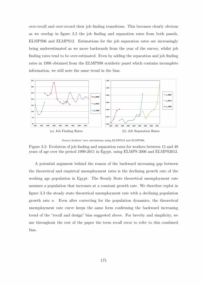
over-recall and over-record their job finding transitions. This becomes clearly obvious

as we overlap in figure 3.2 the job finding and separation rates from both panels,

ELMPS06 and ELMPS12. Estimations for the job separation rates are increasingly

being underestimated as we move backwards from the year of the survey, whilst job

finding rates tend to be over-estimated. Even by adding the separation and job finding

rates in 1998 obtained from the ELMPS98 synthetic panel which contains incomplete

information, we still note the same trend in the bias.

0%

5%

10%

15%

20%

25%

30%

35%

1994 1996 1998 2000 2002 2004 2006 2008 2010

f_2006

f_2012

f_1998

(a) Job Finding Rates

0.00%

0.20%

0.40%

0.60%

0.80%

1.00%

1.20%

1994 1996 1998 2000 2002 2004 2006 2008 2010

s_2006

s_2012

s_1998

(b) Job Separation Rates

Source:Authors’ own calculations using ELMPS12 and ELMPS06.

Figure 3.2: Evolution of job finding and separation rates for workers between 15 and 49years of age over the period 1999-2011 in Egypt, using ELMPS 2006 and ELMPS2012.

A potential argument behind the reason of the backward increasing gap between

the theoretical and empirical unemployment rates is the declining growth rate of the

working age population in Egypt. The Steady State theoretical unemployment rate

assumes a population that increases at a constant growth rate. We therefore replot in

figure 3.3 the steady state theoretical unemployment rate with a declining population

growth rate n. Even after correcting for the population dynamics, the theoretical

unemployment rate curve keeps the same form confirming the backward increasing

trend of the “recall and design” bias suggested above. For brevity and simplicity, we

use throughout the rest of the paper the term recall error to refer to this combined

bias.

175

(a) Working Age Population Growth (b) Steady-State Theoretical UnemploymentRate

Source: Authors’ own calculations using ELMPS12 and ELMPS06.

Figure 3.3: Steady-State unemployment rates, with a constant versus decreasing pop-ulation growth rate, male workers between 15 and 49 years of age.

3.4.2 A Model Correcting Recall Error

We present two models: the first one is a simple two-state model (here employment

and unemployment), and the second is a three-state model (employment, unemploy-

ment and inactivity)14.

A two-state model

We suppose that the true labor market histories are generated by a discrete-time

Markov chain. The vector of the true labor market state occupied at year t is

X(t) =

E(t)

U(t)

(3.3)

where E(t) and U(t) represent the true proportion of employed and unemployed re-

spectively in the labor force in year t. These are therefore the unbiased true moments

14The model can be easily extended to multiple state to be able to correct detailed labor markettransitions, for instance among the different employment sectors and non-employment. However, giventhe nature of the data used and the available samples’ sizes, as has been shown in chapter 1, it is notpossible to estimate a multiple-state model using the longitudinal retrospective panels extracted fromthe ELMPS surveys.

176

of the population stocks obtained from the data. The vector

x(t) =

e(t)u(t)

(3.4)

denotes the observed empirical labor market state proportions at time t, with e(t) and

u(t) being the observed proportion of employed and unemployed in the labor force in

year t. These are the observed moments that decay,i.e. get biased due to the recall and

design measurement errors as one goes back in time from the year of the survey.With

λlk(t − 1, t) being the transition rates from state l occupied in t − 1 to the state k

occupied in t, the matrix

M(t− 1, t) =

λEE(t− 1, t) λEU(t− 1, t)

λUE(t− 1, t) λUU(t− 1, t)

15 (3.5)

gives the observed transition probabilities between the year t− 1 and the year t. These

are obtained by aggregating the expanded number of individuals making the transition

lk from the year t− 1 to year t in the constructed retrospective panels and dividing by

the stock of l in the year t− 1. There exists a restriction on these transition rates: the

sum of the elements of each column must be equal to one,

λEU(t− 1, t) = 1− λEE(t− 1, t) (3.6)

λUE(t− 1, t) = 1− λUU(t− 1, t) (3.7)

The transition matrix in equation 5.14 leads to

x(t) = M ′(t− 1, t)x(t− 1) (3.8)

where M ′(t − 1, t) is the transposed matrix of M(t − 1, t). The observed transition

probabilities, as have been explained above, are biased due to recall and design mea-

surement errors. To be able to correct this bias, an error term ϕz(t−1, t), for z = E,U ,

is defined and associated to the z-type agents. These error terms vary in time and in-

crease as one goes back in history, showing the loss of accuracy and memory as older

177

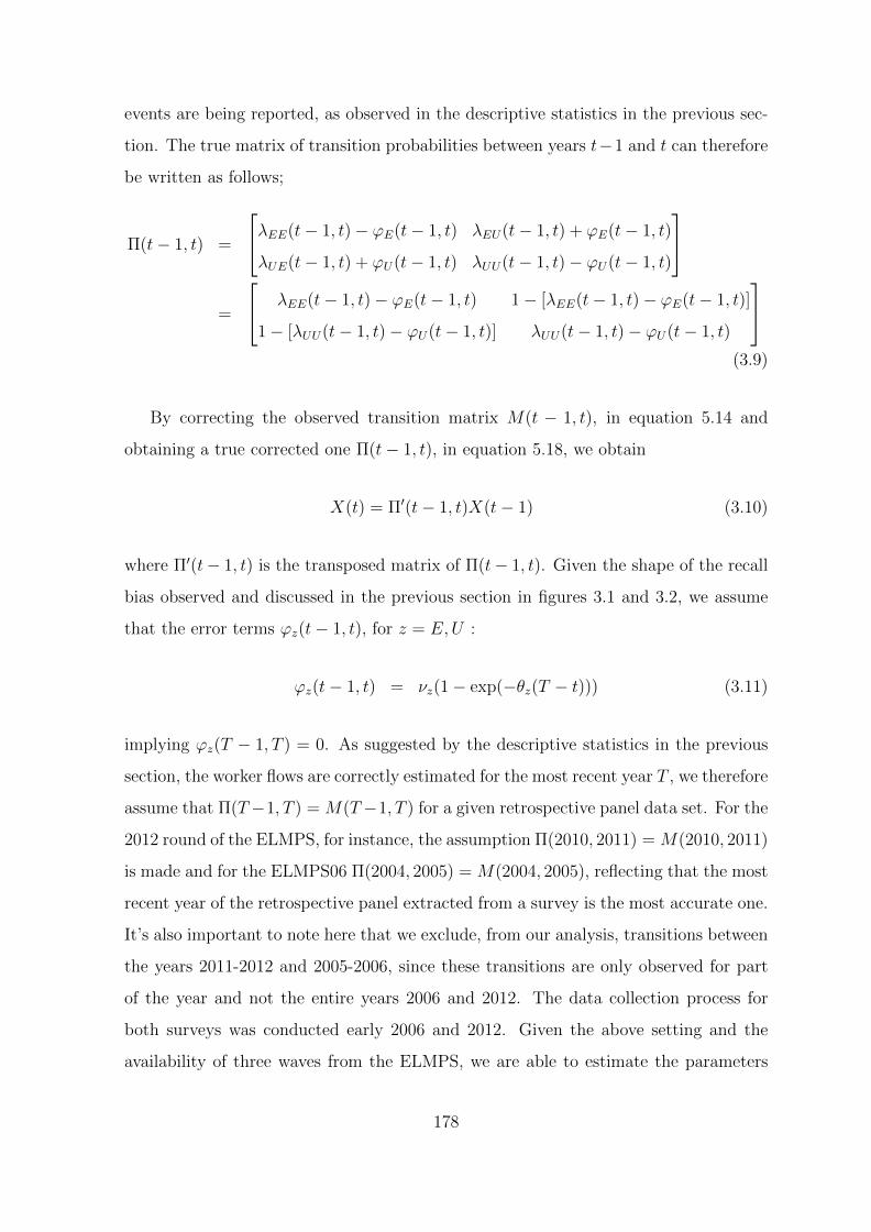
events are being reported, as observed in the descriptive statistics in the previous sec-

tion. The true matrix of transition probabilities between years t−1 and t can therefore

be written as follows;

Π(t− 1, t) =

λEE(t− 1, t)− ϕE(t− 1, t) λEU(t− 1, t) + ϕE(t− 1, t)

λUE(t− 1, t) + ϕU(t− 1, t) λUU(t− 1, t)− ϕU(t− 1, t)

=

λEE(t− 1, t)− ϕE(t− 1, t) 1− [λEE(t− 1, t)− ϕE(t− 1, t)]

1− [λUU(t− 1, t)− ϕU(t− 1, t)] λUU(t− 1, t)− ϕU(t− 1, t)

(3.9)

By correcting the observed transition matrix M(t − 1, t), in equation 5.14 and

obtaining a true corrected one Π(t− 1, t), in equation 5.18, we obtain

X(t) = Π′(t− 1, t)X(t− 1) (3.10)

where Π′(t− 1, t) is the transposed matrix of Π(t− 1, t). Given the shape of the recall

bias observed and discussed in the previous section in figures 3.1 and 3.2, we assume

that the error terms ϕz(t− 1, t), for z = E,U :

ϕz(t− 1, t) = νz(1− exp(−θz(T − t))) (3.11)

implying ϕz(T − 1, T ) = 0. As suggested by the descriptive statistics in the previous

section, the worker flows are correctly estimated for the most recent year T , we therefore

assume that Π(T−1, T ) = M(T−1, T ) for a given retrospective panel data set. For the

2012 round of the ELMPS, for instance, the assumption Π(2010, 2011) = M(2010, 2011)

is made and for the ELMPS06 Π(2004, 2005) = M(2004, 2005), reflecting that the most

recent year of the retrospective panel extracted from a survey is the most accurate one.

It’s also important to note here that we exclude, from our analysis, transitions between

the years 2011-2012 and 2005-2006, since these transitions are only observed for part

of the year and not the entire years 2006 and 2012. The data collection process for

both surveys was conducted early 2006 and 2012. Given the above setting and the

availability of three waves from the ELMPS, we are able to estimate the parameters

178

Θ = θE, θU , νE, νU, using a Simulated Method of Moments (SMM). We solve the

following system

g(xT ,Θ) =

X(2011)ELMPS12

X(2005)ELMPS06

λEE(2004, 2005)|2006

λUU(2004, 2005)|2006

−

Π1(Θ)

Π2(Θ)

Π3(Θ)

Π4(Θ)

= [ψT − ψ(Θ)] (3.12)

where

Π1(Θ) =

(2011∏t=2006

Π′(t− 1, t)

)X(2005)ELMPS06

Π2(Θ) =

(2011∏t=1998

Π′(t− 1, t)

)X(1997)ELMPS98

Π3(Θ) = λEE(2004, 2005)|2012 − νE(1− exp(−θE(2011− 2005)))

Π4(Θ) = λUU(2004, 2005)|2012 − νU(1− exp(−θU(2011− 2005)))

This set of restrictions lead to 4 identifying equations. The fist two line of g(xT ,Θ) are

a 2× 2 system with only one independent equation16,

E(2011) = π1,EEE(2005) + (1− π1,UU)(1− E(2005))

E(2005) = π2,EEE(1997) + (1− π2,UU)(1− E(1997))

The two additional identifying restrictions are given by the 2×2 system leading to two

16These two first lines of g(xT ,Θ) are

E(2011) = π1,EEE(2005) + (1− π1,UU )(1− E(2005))

1− E(2011) = (1− π1,EE)E(2005) + π1,UU (1− E(2005))

E(2005) = π2,EEE(1997) + (1− π2,UU )(1− E(1997))

1− E(2005) = (1− π2,EE)E(1997) + π2,UU (1− E(1998))

where the two first lines lead to the same restriction, as the the two last lines.

179

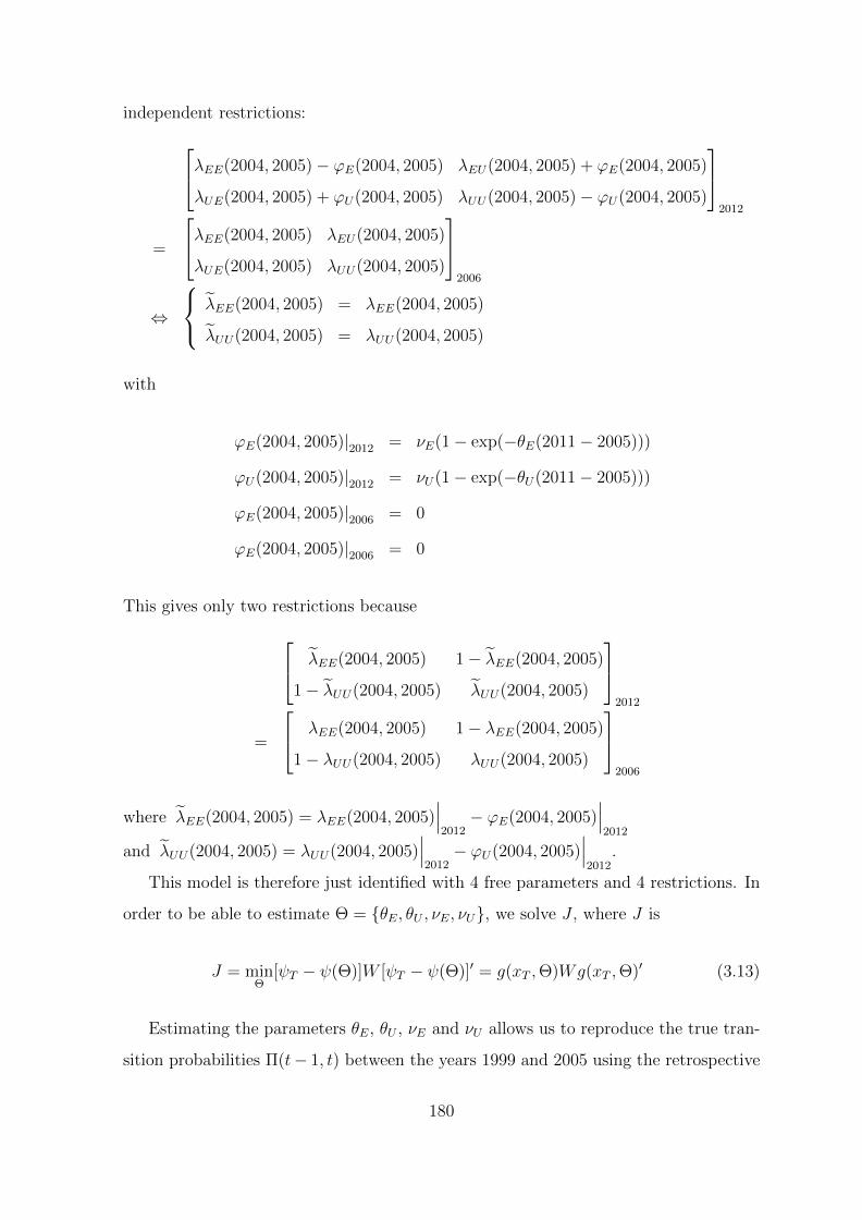
independent restrictions:λEE(2004, 2005)− ϕE(2004, 2005) λEU(2004, 2005) + ϕE(2004, 2005)

λUE(2004, 2005) + ϕU(2004, 2005) λUU(2004, 2005)− ϕU(2004, 2005)

2012

=

λEE(2004, 2005) λEU(2004, 2005)

λUE(2004, 2005) λUU(2004, 2005)

2006

⇔

λEE(2004, 2005) = λEE(2004, 2005)

λUU(2004, 2005) = λUU(2004, 2005)

with

ϕE(2004, 2005)|2012 = νE(1− exp(−θE(2011− 2005)))

ϕU(2004, 2005)|2012 = νU(1− exp(−θU(2011− 2005)))

ϕE(2004, 2005)|2006 = 0

ϕE(2004, 2005)|2006 = 0

This gives only two restrictions because λEE(2004, 2005) 1− λEE(2004, 2005)

1− λUU(2004, 2005) λUU(2004, 2005)

2012

=

λEE(2004, 2005) 1− λEE(2004, 2005)

1− λUU(2004, 2005) λUU(2004, 2005)

2006

where λEE(2004, 2005) = λEE(2004, 2005)∣∣∣2012− ϕE(2004, 2005)

∣∣∣2012

and λUU(2004, 2005) = λUU(2004, 2005)∣∣∣2012− ϕU(2004, 2005)

∣∣∣2012

.

This model is therefore just identified with 4 free parameters and 4 restrictions. In

order to be able to estimate Θ = θE, θU , νE, νU, we solve J , where J is

J = minΘ

[ψT − ψ(Θ)]W [ψT − ψ(Θ)]′ = g(xT ,Θ)Wg(xT ,Θ)′ (3.13)

Estimating the parameters θE, θU , νE and νU allows us to reproduce the true tran-

sition probabilities Π(t− 1, t) between the years 1999 and 2005 using the retrospective

180

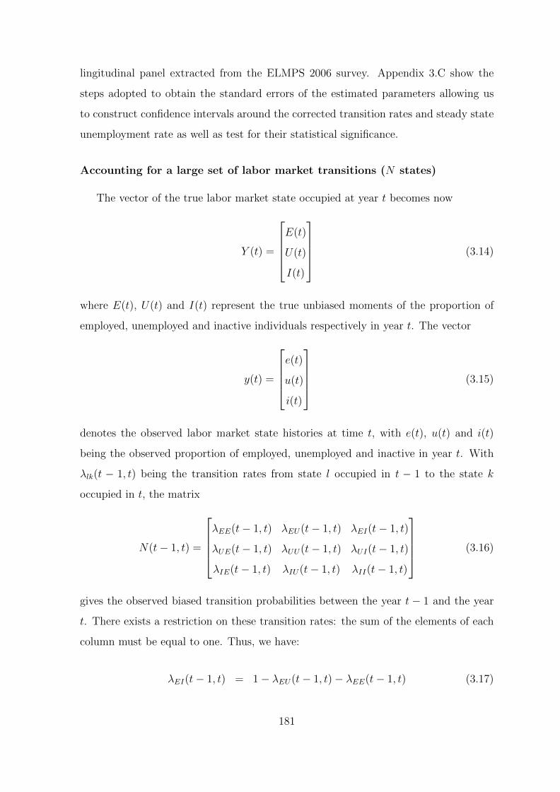
lingitudinal panel extracted from the ELMPS 2006 survey. Appendix 3.C show the

steps adopted to obtain the standard errors of the estimated parameters allowing us

to construct confidence intervals around the corrected transition rates and steady state

unemployment rate as well as test for their statistical significance.

Accounting for a large set of labor market transitions (N states)

The vector of the true labor market state occupied at year t becomes now

Y (t) =

E(t)

U(t)

I(t)

(3.14)

where E(t), U(t) and I(t) represent the true unbiased moments of the proportion of

employed, unemployed and inactive individuals respectively in year t. The vector

y(t) =

e(t)

u(t)

i(t)

(3.15)

denotes the observed labor market state histories at time t, with e(t), u(t) and i(t)

being the observed proportion of employed, unemployed and inactive in year t. With

λlk(t − 1, t) being the transition rates from state l occupied in t − 1 to the state k

occupied in t, the matrix

N(t− 1, t) =

λEE(t− 1, t) λEU(t− 1, t) λEI(t− 1, t)

λUE(t− 1, t) λUU(t− 1, t) λUI(t− 1, t)

λIE(t− 1, t) λIU(t− 1, t) λII(t− 1, t)

(3.16)

gives the observed biased transition probabilities between the year t − 1 and the year

t. There exists a restriction on these transition rates: the sum of the elements of each

column must be equal to one. Thus, we have:

λEI(t− 1, t) = 1− λEU(t− 1, t)− λEE(t− 1, t) (3.17)

181

λUI(t− 1, t) = 1− λUE(t− 1, t)− λUU(t− 1, t) (3.18)

λIU(t− 1, t) = 1− λIE(t− 1, t)− λII(t− 1, t) (3.19)

This transition matrix leads to

y(t) = N ′(t− 1, t)y(t− 1) (3.20)

As previously, the observation of the transition probabilities can be biased due to the

recall error. To correct this bias, we propose to estimate, in this case, three functions,

one for each subgroup. We define ϕz(t − 1, t), for z = E,U, I, as the associated error

terms to the z-type agents (the subgroup). These errors also vary in time and increase

as we go back in history. Again, these simply reflect that people tend to lose accuracy

and memory as they report older events. This allows us to write the true matrix of

transition probabilities between years t− 1 and t as follows;

Ω(t− 1, t) =

λEE − ϕE λEU + a1ϕE λEI + (1− a1)ϕE

λUE + b1ϕU λUU − ϕU λUI + (1− b1)ϕg

λIE + c1ϕI λIU + (1− c1)ϕI λII − ϕI

λEE − ϕE λEU + a1ϕE (1− λEE − λEU) + (1− a1)ϕE

λUE + b1ϕU λUU − ϕU (1− λUE − λUU) + (1− b1)ϕU

λIE + c1ϕI (1− λIE − λII) + (1− c1)ϕI λII − ϕI

(3.21)

With the correction, we obtain

Y (t) = Ω′(t− 1, t)Y (t) (3.22)

As in the two state model, the error terms ϕz(t−1, t) are assumed to have the following

functional forms:

ϕz(t− 1, t) = νz(1− exp(−θz(T − t)))

182

implying ϕz(T − 1, T ) = 0. Since as we show in the previous section, our worker

flows are correctly estimated for the most recent year T , we therefore assume that

Ω(T − 1, T ) = N(T − 1, T ) for a given synthetic panel data set. This implies that for

the ELMPS12 constructed panel Ω(2010, 2011) = N(2010, 2011) and for the ELMPS06

Ω(2004, 2005) = N(2004, 2005). Given this new three-state setting, we are now able to

estimate the parameters

Θ3 = θE, θU , θI , νE, νU , νI , a1, b1, c1

where dim(Θ3) = 9, by solving the following system

g(xT ,Θ3) =

Y (2011)ELMPS12

Y (2005)ELMPS06

λEE(2004, 2005)|2006

λUU(2004, 2005)|2006

λII(2004, 2005)|2006

λEU(2004, 2005)|2006

λUE(2004, 2005)|2006

λIE(2004, 2005)|2006

−

Ω1(Θ3)

Ω2(Θ3)

Ω3(Θ3)

Ω4(Θ3)

Ω5(Θ3)

Ω6(Θ3)

Ω7(Θ3)

Ω8(Θ3)

= [ψT − ψ(Θ3)] (3.23)

183

where

Ω1(Θ3) =

(2011∏t=2006

Ω′(t− 1, t)

)Y (2005)ELMPS06

Ω2(Θ3) =

(2011∏t=1998

Ω′(t− 1, t)

)Y (1997)ELMPS98

Ω3(Θ3) = λEE(2004, 2005)|2012 − νE(1− exp(−θE(2011− 2005)))

Ω4(Θ3) = λUU(2004, 2005)|2012 − νU(1− exp(−θU(2011− 2005)))

Ω5(Θ3) = λII(2004, 2005)|2012 − νI(1− exp(−θI(2011− 2005)))

Ω6(Θ3) = λEU(2004, 2005)|2012 − νE(1− exp(−θE(2011− 2005)))

Ω7(Θ3) = λUE(2004, 2005)|2012 − νU(1− exp(−θU(2011− 2005)))

Ω8(Θ3) = λIE(2004, 2005)|2012 − νI(1− exp(−θI(2011− 2005)))

Similar to the derivation done for the two state model, we therefore find out that the

identification of Ω relies on restrictions laid out by equations that serve to guarantee

the consistency of Ω with the evolution of stocks between 2005 and 2011 as well as 1997

and 2005. Since 1 = E + U + I, these would yield 4 restrictions only allowing us to

identify only four free parameters. We therefore add six more restrictions identified by

Ω(2004, 2005)ELMPS06 = Ω(2004, 2005)ELMPS12

The relations between the transition rates in equations 3.17, 3.18 and 3.19 is the reason

that we only yield six restrictions. Given the structure imposed by the three states

model, we have ten restrictions and nine free parameters: the model is therefore over-

identified. Further tests after estimation can therefore be developed in this case to test

for its goodness of fit.

The same estimation methodology, as for the two-state model, is adopted where to

estimate Θ = θE, θU , θI , νE, νU , νI, we solve J , where J is

J = minΘ3

[ψT − ψ(Θ3)]W [ψT − ψ(Θ3)]′ = g(xT ,Θ3)Wg(xT ,Θ3)′ (3.24)

We use our estimated θz, νz, a1, b1 and c1, for z = E,U, I, to reproduce the

184

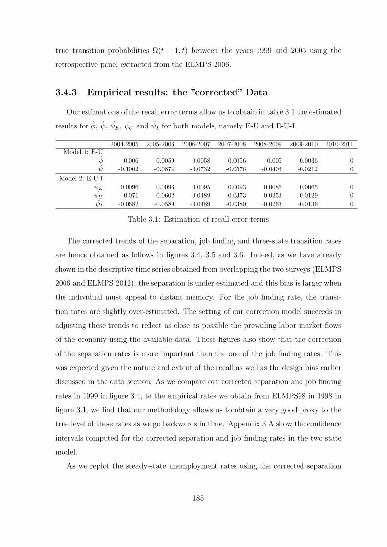
true transition probabilities Ω(t − 1, t) between the years 1999 and 2005 using the

retrospective panel extracted from the ELMPS 2006.

3.4.3 Empirical results: the ”corrected” Data

Our estimations of the recall error terms allow us to obtain in table 3.1 the estimated

results for φ, ψ, ψE, ψU and ψI for both models, namely E-U and E-U-I.

2004-2005 2005-2006 2006-2007 2007-2008 2008-2009 2009-2010 2010-2011Model 1: E-U

φ 0.006 0.0059 0.0058 0.0056 0.005 0.0036 0

ψ -0.1002 -0.0874 -0.0732 -0.0576 -0.0403 -0.0212 0

Model 2: E-U-I

ψE 0.0096 0.0096 0.0095 0.0093 0.0086 0.0065 0

ψU -0.071 -0.0602 -0.0489 -0.0373 -0.0253 -0.0129 0

ψI -0.0682 -0.0589 -0.0489 -0.0380 -0.0263 -0.0136 0

Table 3.1: Estimation of recall error terms

The corrected trends of the separation, job finding and three-state transition rates

are hence obtained as follows in figures 3.4, 3.5 and 3.6. Indeed, as we have already

shown in the descriptive time series obtained from overlapping the two surveys (ELMPS

2006 and ELMPS 2012), the separation is under-estimated and this bias is larger when

the individual must appeal to distant memory. For the job finding rate, the transi-

tion rates are slightly over-estimated. The setting of our correction model succeeds in

adjusting these trends to reflect as close as possible the prevailing labor market flows

of the economy using the available data. These figures also show that the correction

of the separation rates is more important than the one of the job finding rates. This

was expected given the nature and extent of the recall as well as the design bias earlier

discussed in the data section. As we compare our corrected separation and job finding

rates in 1999 in figure 3.4, to the empirical rates we obtain from ELMPS98 in 1998 in

figure 3.1, we find that our methodology allows us to obtain a very good proxy to the

true level of these rates as we go backwards in time. Appendix 3.A show the confidence

intervals computed for the corrected separation and job finding rates in the two state

model.

As we replot the steady-state unemployment rates using the corrected separation

185

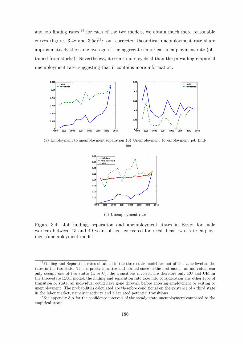
and job finding rates 17 for each of the two models, we obtain much more reasonable

curves (figures 3.4c and 3.5c)18: our corrected theoretical unemployment rate share

approximatively the same average of the aggregate empirical unemployment rate (ob-

tained from stocks). Nevertheless, it seems more cyclical than the prevailing empirical

unemployment rate, suggesting that it contains more information.

1998 2000 2002 2004 2006 2008 2010 20120

0.002

0.004

0.006

0.008

0.01

0.012

data

corrected

(a) Employment to unemployment separation

1998 2000 2002 2004 2006 2008 2010 20120.1

0.15

0.2

0.25

0.3

0.35

data

corrected

(b) Unemployment to employment job find-ing

1998 2000 2002 2004 2006 2008 2010 20120

0.01

0.02

0.03

0.04

0.05

0.06

0.07

0.08

SS data

SS corrected

data

(c) Unemployment rate

Figure 3.4: Job finding, separation and unemployment Rates in Egypt for maleworkers between 15 and 49 years of age, corrected for recall bias, two-state employ-ment/unemployment model

17Finding and Separation rates obtained in the three-state model are not of the same level as therates in the two-state. This is pretty intuitive and normal since in the first model, an individual canonly occupy one of two states (E or U), the transitions involved are therefore only EU and UE. Inthe three-state E,U,I model, the finding and separation rate take into consideration any other type oftransition or state, an individual could have gone through before entering employment or exiting tounemployment. The probabilities calculated are therefore conditional on the existence of a third statein the labor market, namely inactivity and all related potential transitions.

18See appendix 3.A for the confidence intervals of the steady state unemployment compared to theempirical stocks

186

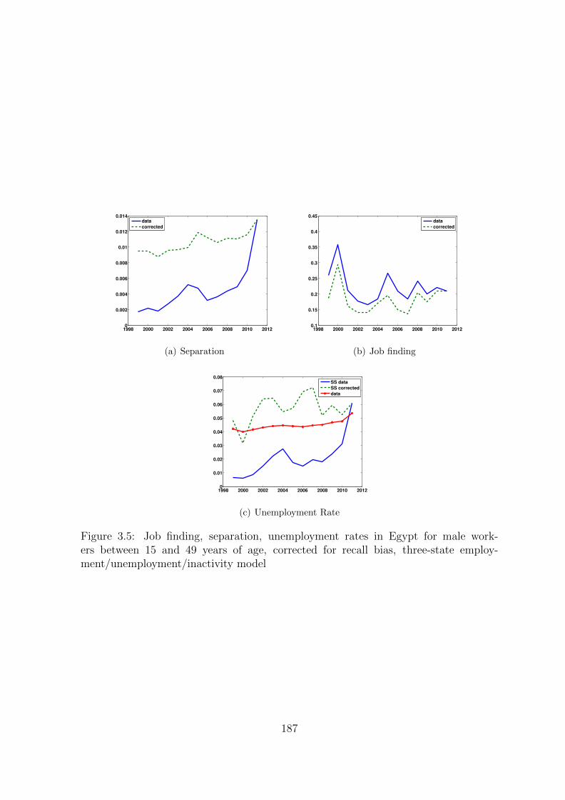
1998 2000 2002 2004 2006 2008 2010 20120

0.002

0.004

0.006

0.008

0.01

0.012

0.014

data

corrected

(a) Separation

1998 2000 2002 2004 2006 2008 2010 20120.1

0.15

0.2

0.25

0.3

0.35

0.4

0.45

data

corrected

(b) Job finding

1998 2000 2002 2004 2006 2008 2010 20120

0.01

0.02

0.03

0.04

0.05

0.06

0.07

0.08

SS data

SS corrected

data

(c) Unemployment Rate

Figure 3.5: Job finding, separation, unemployment rates in Egypt for male work-ers between 15 and 49 years of age, corrected for recall bias, three-state employ-ment/unemployment/inactivity model

187

1998 2000 2002 2004 2006 2008 2010 20120.978

0.98

0.982

0.984

0.986

0.988

0.99

0.992

0.994

0.996

0.998

data

corrected

(a) ΛEE

1998 2000 2002 2004 2006 2008 2010 20120

0.002

0.004

0.006

0.008

0.01

0.012

data

corrected

(b) ΛEU

1998 2000 2002 2004 2006 2008 2010 20120.004

0.006

0.008

0.01

0.012

0.014

0.016

data

corrected

(c) ΛEI

1998 2000 2002 2004 2006 2008 2010 20120.12

0.14

0.16

0.18

0.2

0.22

0.24

0.26

0.28

0.3

0.32

data

corrected

(d) ΛUE

1998 2000 2002 2004 2006 2008 2010 2012

0.65

0.7

0.75

0.8

0.85

0.9

0.95

data

corrected

(e) ΛUU

1998 2000 2002 2004 2006 2008 2010 20120

0.01

0.02

0.03

0.04

0.05

0.06

data

corrected

(f) ΛUI

1998 2000 2002 2004 2006 2008 2010 20120.04

0.06

0.08

0.1

0.12

0.14

0.16

0.18

data

corrected

(g) ΛIE

1998 2000 2002 2004 2006 2008 2010 20120.02

0.025

0.03

0.035

0.04

0.045

data

corrected

(h) ΛIU

1998 2000 2002 2004 2006 2008 2010 20120.8

0.82

0.84

0.86

0.88

0.9

0.92

0.94

data

corrected

(i) ΛII

Figure 3.6: All transition rates in Egypt for male workers between 15 and 49 years ofage, corrected for recall bias, three-state employment/unemployment/inactivity model

188

3.5 Policy Evaluation of the reform

In this section, our objective is to detect a structural break, linked to a permanent

and unexpected change in the labor market policy. We first present our simple econo-

metric methodology allowing us to identify a permanent change linked to the reform,

and then, we present and comment our empirical findings.

3.5.1 Econometric Methodology

A two-state labor market. In our time series, there are two components. The

first one accounts for the business cycle, whereas the second accounts for long run

component. Only this last part matters for our analysis. It is therefore necessary to

purge the time series from their cyclical components. We extract the high frequency

component of each series using the first difference of the observed output (in log):

our final data are then the trend of the original time obtained after a projection on

aggregate business cycle measures: we obtain a measure of the long run components

of the worker flows. We test the robustness of your statistical approach by using the

cyclical component of the output (in log) extracted by the Hodrick-Prescott (HP) filter

instead to use the first difference of the output.

Any policy, that changes the natural rate of the worker flows (x?), introduces an

instability on the relation

xt = b+ Iaγ + εt for x = f, s.

This allows us to test the impact of the 2003 reform in the Egyptian labor market.

Without any observed policy change (γ = 0), the variations in xt are driven by un-

observable changes in the matching and the separation processes. Remark that the

time series xst , built under the assumption of a stable relationship over time, can be

interpreted as the counterfactual of an economy without any policy changes (this time

series is build with γ = 0). If the policy change the natural rate of the worker flows,

then the “true” series of the natural worker flows are given by xt. The gap between xt

and xst measures the impact of the reform.

189

Given that the unemployment rate is well approximated by its stationary value at

the flow equilibrium, we can use our estimations of the natural flows to construct the

implied natural unemployment. More formally, we have u = ss+f

. Thus, if we only

focus on the component of the worker flows purged from the cyclical component linked

to the GDP, we have ut = stst+ft

and ust =sst

sst+fst.

Finally, in order to measure the relative contribution of the worker flows in the

unemployment dynamics, one can compute uft = stst+fst

: this time series gives the un-

employment dynamics if only the job finding rate is affected by the reform, or in other

words, the contribution of the change in the job finding rate to the natural unemploy-

ment variation.

Extension: Entry and exit from the labor force. In a developing rigid labor

market such as Egypt, flows to and from inactivity play an important role as a determi-

nant of final labor market outcomes. Examining the gross flows of workers, between the

three labor market states, employment (E), unemployment (U) and inactivity, becomes

essential to portray as fully as possible the real story and the particular nature of the

market.

In such case we adopt the same econometric methodology described above to mea-

sure the impact of the 2003 new labor law on the three-state labor market transitions.

However, as mentioned previously, we now have a 3 × 3 matrix of the corrected tran-

sition probabilities, Ω(t − 1, t). With Λji(t − 1, t) being the corrected transition rates

from state j occupied in t − 1 to the state i occupied in t, we re-write Ω(t − 1, t) as

follows;

Ω(t− 1, t) =

ΛEE ΛEU ΛEI

ΛUE ΛUU ΛUI

ΛIE ΛIU ΛII

This therefore extract the cyclical component of the workers flows using the first dif-

ference of the observed output (in log)19, and we analyze the behavior of the ”natural”

19As previously, a robustness check is provided by the use of the HP filter instead of the firstdifference of the output.

190

rate of worker flows using the model

xt = b+ Iaγ + εt for x = ΛEE,ΛEU ,ΛEI ,ΛUE,ΛUU ,ΛUI ,ΛIE,ΛIU ,ΛII .

This allows us to test if the policy changes the natural rate of the worker flows or not.

We then use our estimations of the natural flows to construct the implied natural

unemployment. Following Shimer (2012), in a three-state E-U-I model, the number

of employed, unemployed and inactive individuals are determined by the following

equations;

E = k(ΛUIΛIE + ΛIUΛUE + ΛIEΛUE)

U = k(ΛEIΛIU + ΛIEΛEU + ΛIUΛEU)

I = k(ΛEUΛUI + ΛUEΛEI + ΛUIΛEI)

where k is a constant set so that E, U and I sum to the relevant population. The

steady-state unemployment rate (u = ss+f

) in a three-state labor market can therefore

be written as

u =ΛEIΛIU + ΛIEΛEU + ΛIUΛEU

(ΛEIΛIU + ΛIEΛEU + ΛIUΛEU) + (ΛUIΛIE + ΛIUΛUE + ΛIEΛUE)

The relative contribution of the worker flows in the unemployment dynamics is then

calculated. One can compute uft = stst+fst

, a time series that gives the unemployment

dynamics if only job finding rate is affected by the reform given no change in the

separation rates. In the three-state model (where individuals can also be inactive), the

separation and job finding rates take into account all intermediate states/transitions, an

individual could have gone through before exiting into unemployment or entering into

employment. The hypothetical separation and job finding rates are therefore calculated

as follows;

st = ΛEIΛIU + ΛIEΛEU + ΛIUΛEU

f st = ΛUIΛIE + ΛIUΛUE + ΛIEΛUE.

In other words, we show the unemployment dynamics if the three-state model separa-

191

tion rate followed the same dynamics as before the 2003 reform.

3.5.2 Estimation and Results

In this section, we show that correcting for the recall bias enables us, to investigate

the ”true”evolution of worker flows trends over the period 1998-2012 in our both models;

E-U and E-U-I. To illustrate the interest of our approach, we propose, in a first ”naive”

estimation, the impact of the reform suing non-corrected data. In a second step, using

the corrected data, we provide a more robust analysis. We are then able to link changes

in the job finding and separation rates to the 2003 New Labor Law implemented in

Egypt in 2004.

A Naive Econometric Model

In a naive econometric scenario, the above recall error would be neglected: the

data used in this ”naive” approach are the non-corrected data. The job finding and

separation rates are purged from their business cycle component. In order to account

for the increase of the recall bias, we also introduce a linear and a quadratic trend: this

is the ”naive” method which allows this simple econometric model to have stationary

residuals, given the shape of the non-corrected time series of separation and job finding

rates. We hence use the following econometric model:

xt = β1t+ β2t2 + b+ Iaγ + εt for x = f, s

where ft and st are respectively the observed job finding and job separation rates. β1

and β2 are two constants representing the linear and quadratic trends (in our case

the increasing slope) of the time series. b is a constant term that encompasses the

“true” constant and the structural rate of worker flows (hiring or separation). We also

introduce a dummy Ia = 1 after the reform and 0 before. By running such a regression,

one obtains the following results reported in table 3.2.

By neglecting the recall error, or more precisely, by using a reduced form analysis

which does not use the restrictions provided by the data and the stock-flow models,

the law seems to have reduced the unemployment rate. There has been a significant

192

f f s sβ1 -0.0360** -0.0348 -0.000028 0.000214β2 0.0025* 0.0035 0.000042** 0.00044***b 0.2534*** 0.2253* 0.0017** -0.0004γ -0.0310 -0.002337***

Table 3.2: OLS regression results, a naive econometric model

decrease in the separation rates and non-significant effect on the job finding rates. In

such a case, the law seems inefficient in terms of flexibilizing the labor market, i.e. fa-

cilitating the hiring and firing process. Yet, the policy makers would be relieved seeing

the unemployment rates reduced (see the section 3.6 for a figure of this unsatisfying

correction of the unemployment rate). Unfortunately, the above naive scenario does

not reflect not even part of the reality. By neglecting the structural interaction between

the job finding and separation rates, and detrending each time series apart, one ob-

tains misleading results: some data restrictions are not used in order to constraint the

estimation. We show in the rest of the paper the impact of the reform after correcting

for this recall bias given the underlying interaction between the structural stock-flow

approach of the labor market model and the data.

1998 2000 2002 2004 2006 2008 20100

0.5

1

1.5

2

2.5

3

3.5 x 10−3 Job separation rate

without reformwith reform

(a) Separation rate

1998 2000 2002 2004 2006 2008 20100.06

0.08

0.1

0.12

0.14

0.16

0.18

0.2

0.22Job finding rate

without reformwith reform

(b) Job finding rate

Figure 3.7: Job Finding and Separation Rates with and without the new labor marketreform in 2004, a naive econometric model

The evaluation of the reform with corrected data

After correcting the labor market flows from the recall error, we compute the steady-

state unemployment rate (u = ss+f

), our proxy to the prevailing unemployment rate

193

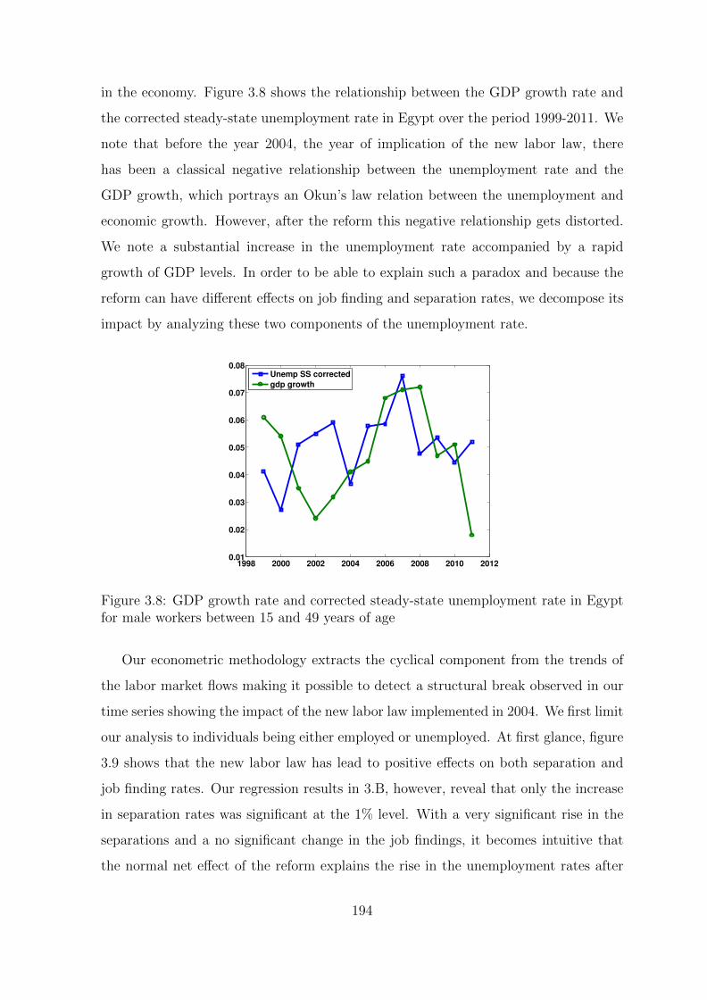
in the economy. Figure 3.8 shows the relationship between the GDP growth rate and

the corrected steady-state unemployment rate in Egypt over the period 1999-2011. We

note that before the year 2004, the year of implication of the new labor law, there

has been a classical negative relationship between the unemployment rate and the

GDP growth, which portrays an Okun’s law relation between the unemployment and

economic growth. However, after the reform this negative relationship gets distorted.

We note a substantial increase in the unemployment rate accompanied by a rapid

growth of GDP levels. In order to be able to explain such a paradox and because the

reform can have different effects on job finding and separation rates, we decompose its

impact by analyzing these two components of the unemployment rate.

1998 2000 2002 2004 2006 2008 2010 20120.01

0.02

0.03

0.04

0.05

0.06

0.07

0.08

Unemp SS corrected

gdp growth

Figure 3.8: GDP growth rate and corrected steady-state unemployment rate in Egyptfor male workers between 15 and 49 years of age

Our econometric methodology extracts the cyclical component from the trends of

the labor market flows making it possible to detect a structural break observed in our

time series showing the impact of the new labor law implemented in 2004. We first limit

our analysis to individuals being either employed or unemployed. At first glance, figure

3.9 shows that the new labor law has lead to positive effects on both separation and

job finding rates. Our regression results in 3.B, however, reveal that only the increase

in separation rates was significant at the 1% level. With a very significant rise in the

separations and a no significant change in the job findings, it becomes intuitive that

the normal net effect of the reform explains the rise in the unemployment rates after

194

2004.

1998 2000 2002 2004 2006 2008 2010 20120.007

0.008

0.009

0.01

0.011

0.012

0.013

0.014

without reform

with reform

(a) E-to-U separation rate

1998 2000 2002 2004 2006 2008 2010 20120.1

0.12

0.14

0.16

0.18

0.2

0.22

0.24

0.26

without reform

with reform

(b) U-to-E job finding rate

Figure 3.9: Trends of Job Finding and Separation Rates with and without the newlabor market reform in 2004, a two-state E/U model

The full story of the Egyptian labor market is never however complete as one ex-

cludes flows entering and exiting the labor force. According to Yassine (2014), the

new entrants (inactivity to employment) constitute a substantial flow of workers, that

one can not ignore when analyzing the Egyptian labor market. As a matter of fact it

has been argued that, being a developing country, looking at participation rates might

portray a better picture of the health of the labor market. Consequently, the detrended

job finding and separation rates are reconstructed but this time for a three-state model

where individuals can either be employed, unemployed or inactive. By modeling all

possible labor market flows, we calculate separation and job finding rates, but this

time accounting for the existence of the inactivity state. Our results are robust and

coherent with the two-state E/U system. The 2003 reform lead to a significant increase

in the separation rates and barely any impact on the job finding rates. Looking at

the more detailed labor market transitions, we show that even though the structural

break, observed in 2004, favored the unemployment-to-employment (ΛUE) flows, as well

as inactivity-to-employment (ΛIE) labor market flows, the impact has been insignifi-

cant for both (The coefficients when (γ 6= 0) were insignificant for these flows.). The

introduction of the dummy at the time of the reform neither improved the fit of the

regressions for (ΛIE) nor (ΛUE). On the other hand, the coefficients of the dummy γ

for the regressions of (ΛEI) and (ΛEU) were statistically significant (Table 3.5). It’s im-

195

portant to note at this point that the E-to-I has been slightly affected negatively after

the 2003 law. This impact was only significant at the 10% level and was mainly domi-

nated by the very significant increment of the E-to-U flows. All regressions’ estimations

used in this section are illustrated in appendix 3.B. We also redo our regressions, by

detrending our flows using the Hodrick and Prescott (1997) filter, in the appendix 3.B,

showing that we obtain the same robust results.

In general, we note that the residuals of the regressions that omit the 2003 reform

are non-stationary. For the significant cases (especially separations), the residuals be-

come centered around zero when the reform is taken into account. This supports the

significant impact of the dummy variable reported in the tables 3.3, 3.4 and 3.5.

1998 2000 2002 2004 2006 2008 2010 20120.0095

0.01

0.0105

0.011

0.0115

0.012

0.0125

0.013

0.0135

0.014

0.0145

without reform

with reform

(a) Separation rate

1998 2000 2002 2004 2006 2008 2010 20120.1

0.15

0.2

0.25

0.3

0.35

without reform

with reform

(b) Job finding rate

Figure 3.10: Job Finding and Separation Rates with and without the new labor marketreform in 2004, a three-state E-U-I model

196

1998 2000 2002 2004 2006 2008 2010 20120.978

0.979

0.98

0.981

0.982

0.983

0.984

0.985

without reform

with reform

(a) ΛEE

1998 2000 2002 2004 2006 2008 2010 20120.007

0.008

0.009

0.01

0.011

0.012

0.013

0.014

without reform

with reform

(b) ΛEU

1998 2000 2002 2004 2006 2008 2010 20120.006

0.007

0.008

0.009

0.01

0.011

0.012

0.013

0.014

without reform

with reform

(c) ΛEI

1998 2000 2002 2004 2006 2008 2010 20120.1

0.12

0.14

0.16

0.18

0.2

0.22

0.24

0.26

without reform

with reform

(d) ΛUE

1998 2000 2002 2004 2006 2008 2010 20120.7

0.75

0.8

0.85

0.9

0.95

without reform

with reform

(e) ΛUU

1998 2000 2002 2004 2006 2008 2010 2012−0.02

−0.01

0

0.01

0.02

0.03

0.04

without reform

with reform

(f) ΛUI

1998 2000 2002 2004 2006 2008 2010 20120.075

0.08

0.085

0.09

0.095

0.1

0.105

0.11

0.115

0.12

0.125

without reform

with reform

(g) ΛIE

1998 2000 2002 2004 2006 2008 2010 20120.02

0.025

0.03

0.035

0.04

0.045

without reform

with reform

(h) ΛIU

1998 2000 2002 2004 2006 2008 2010 20120.83

0.84

0.85

0.86

0.87

0.88

0.89

0.9

0.91

without reform

with reform

(i) ΛII

Figure 3.11: Trends of labor market transition rates with and without the new labormarket reform in 2004, a three-state E-U-I model

197

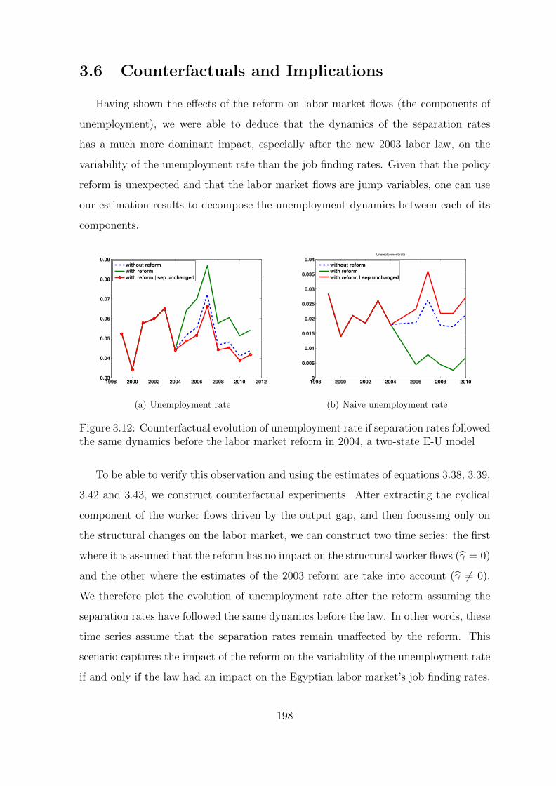
3.6 Counterfactuals and Implications

Having shown the effects of the reform on labor market flows (the components of

unemployment), we were able to deduce that the dynamics of the separation rates

has a much more dominant impact, especially after the new 2003 labor law, on the

variability of the unemployment rate than the job finding rates. Given that the policy

reform is unexpected and that the labor market flows are jump variables, one can use

our estimation results to decompose the unemployment dynamics between each of its

components.

1998 2000 2002 2004 2006 2008 2010 20120.03

0.04

0.05

0.06

0.07

0.08

0.09

without reform

with reform

with reform | sep unchanged

(a) Unemployment rate

1998 2000 2002 2004 2006 2008 20100

0.005

0.01

0.015

0.02

0.025

0.03

0.035

0.04Unemployment rate

without reformwith reformwith reform | sep unchanged

(b) Naive unemployment rate

Figure 3.12: Counterfactual evolution of unemployment rate if separation rates followedthe same dynamics before the labor market reform in 2004, a two-state E-U model

To be able to verify this observation and using the estimates of equations 3.38, 3.39,

3.42 and 3.43, we construct counterfactual experiments. After extracting the cyclical

component of the worker flows driven by the output gap, and then focussing only on

the structural changes on the labor market, we can construct two time series: the first

where it is assumed that the reform has no impact on the structural worker flows (γ = 0)

and the other where the estimates of the 2003 reform are take into account (γ 6= 0).

We therefore plot the evolution of unemployment rate after the reform assuming the

separation rates have followed the same dynamics before the law. In other words, these

time series assume that the separation rates remain unaffected by the reform. This

scenario captures the impact of the reform on the variability of the unemployment rate

if and only if the law had an impact on the Egyptian labor market’s job finding rates.

198

We reproduce the same exercise with the ”naive” econometric model presented in the

section 3.5.2.20 The two panels of figure 3.12 show that the use of the corrected data,

that take into account the restrictions of the markovian processes of the workers flows,

does not lead to the same predictions of a reduced form estimation. Our correction

clearly matters, even for a policy evaluation.

Figures 3.12 and 3.13 show that, whether we take into consideration the existence

of a third state of inactivity in the market or not, the relative contribution of the sep-

aration rates to the Egyptian unemployment dynamics is substantial and significant.

The structural increase in the unemployment rates after the reform is mainly due to

the increase in separation rates. The positive responses (decrease in unemployment)

due to the insignificant increase in the job finding rates were definitely outweighed by

the significant impact of the augmented separations (figure 3.12). Adding inactivity as

a third state in the economy, the positive impact of the job findings on the unemploy-

ment is no more observed (since job findings hardly changed in this model) and all the

unemployment variations are attributed to the separations increase in this case. The

Egyptian unemployment rate was therefore more responsive and had a larger elasticity

vis-a-vis the variation in the level of the separation rate. It is true that it’s important

for an economy, in order to promote higher productivity levels associated with economic

growth, to increase job destruction (i.e separations). This phenomenon should however

be accompanied by new productive jobs being created in a much greater magnitude;

in other words a more proportional increase in the job findings. This assures a healthy

dynamic labor market with natural unemployment rates maintained at low levels. Gen-

erally, the law achieved only part of its double-sided mission, where the firing process

was to some extent facilitated. Yet it has not been offset by a sufficiently increased

and facilitated hiring. As a matter of fact, the law did not affect by any means the

hiring process in the Egyptian labor market. In simple words, more jobs were being

destructed, than before the law, while the same number of jobs were being created.

A normal consequence would be a rise in the unemployment even if the economy has

been experiencing rising rates of economic growth.

20Given the non-stationarity of the uncorrected job flows data, the average of the job finding andseparation rates are x = 1

T

∑t(β1t+ β2t

2) + b.

199

1998 2000 2002 2004 2006 2008 2010 20120.03

0.04

0.05

0.06

0.07

0.08

0.09

0.1

without reform

with reform

with reform | sep unchanged

Figure 3.13: Counterfactual evolution of unemployment rate if separation rates followedthe same dynamics before the labor market reform in 2004, a three-state E-U-I model

3.7 A theoretical attempt to evaluate the partial

failure of the reform

In this section, we survey the conventional Mortensen and Pissarides (1994) theo-

retical model, showing the impact of a reduction of firing costs on the labor market’s

equilibrium. According to the model, the introduction of such reform, modelled as a

decrease in the firing taxes, would lead to the increase of both separation and job find-

ing rates. These theoretical predictions supports the liberalization of the labor market.

Nevertheless, according to our empirical results, following the introduction of a more

flexible employment protection policy in the market, only the job separations in Egypt

increased while the job findings remain unchanged. We therefore try to explain this

phenomenon using the theoretical model. We show that an increase in corruption can

explain the partial failure of the reform.

3.7.1 Setting the Model

We set an equilibrium search model with a matching function m(v, u) that charac-

terizes the search and recruiting process by which new job-worker matches are created.

The recruiting intensities across employers and workers are the same. The matching

function is characterized by constant returns where m(v, u) = m(1, uv)v ≡ q(θ)v with

200

θ = vu

being the market tightness. A vacant job is filled at a rate q(θ); this rate de-

creases in θ since q(θ) = m(1, 1θ). Consequently with increasing market tightness, the

vacancy takes longer to be filled (duration of the vacancy = 1q(θ)

). A worker finds a

job at a rate θq(θ), which increases with θ. It follows that with increased labor market

tightness, a worker takes a shorter duration to find a job (duration of being unemployed

= 1θq(θ)

).

An existing match is destroyed if the idiosyncratic productivity falls below a reserva-

tion threshold, an endogenous variable R. It therefore follows that the unemployment

incidence (E→U) is given by λF (R). If R increases, extra jobs will fall below the

productivity threshold and λF (R) increases. The expected duration of a job is 1λF (R)

.

At steady-state, we have u = λF (R)(1− u)− θq(θ)u = 0. Steady-state unemploy-

ment rate can therefore be expressed as follows: u = λF (R)λF (R)+θq(θ)

= ss+f

. As θ increases,

the steady state unemployment decreases. As the reservation product pR increases (p

being a worker’s skill), more separations take place and the steady state unemployment

increases.

A firm incurs two types of costs and they both increase as the skill sophistica-

tion/level becomes higher: (i) a set-up cost: pC (these are sunk up costs once the

match is formed), and (i) a recruiting cost cp.

An employer and a worker meet, they bargain and agree on an initial wage w0(p).

The job is created, production occurs until they get a shock and that’s when they

renegotiate a wage w(x, p). If x ever falls below the reservation product, that’s when

the job is destructed. The firm pays a firing cost pT (imposed by the employment

protection regulation). This increases with the skill of the worker because it costs more

to get rid of a skilled worker than a less skilled one.

Firm Values

The value of a continuing match to the employer

rJ(x) = px− w(x) + λ

∫ 1

R

[J(z)− J(x)]dF (z) + λF (R)[V − pT − J(x)] (3.25)

201

The asset pricing equation of the present value of an unfilled vacancy is :

rV = q(θ)[J0 − V − pC]− pc (3.26)

Initial value of the match to the employer:

rJ0 = p− w0 + λ

∫ 1

R

[J(z)− J0]dF (z) + λF (R)[V − pT − J0] (3.27)

New vacancies are posted until the capital value of holding a vacancy is equal to zero.

i.e. replace V = 0 in equation 3.26

J0 =pc

q(θ)+ pC (3.28)

This represents that , at the free-entry condition, the cost of recruiting and hiring a

worker should be equal to the anticipated discounted profit the employer gets from the

job.

Worker Values

The value of the worker for the initial and the continuing matches are:

rW0 = w0 + λ

∫ 1

R

[(W (z)−W0]dF (z) + λF (R)[U −W0] (3.29)

rW (x) = w(x) + λ

∫ 1

R

[(W (z)−W (x)]dF (z) + λF (R)[U −W (x)] (3.30)

Value of being unemployed:

rU = b+ θq(θ)[W0 − U ] (3.31)

Wage Determination and Nash Bargaining

The threatpoint is looking for an alternative match partner. β is the worker’s

bargaining power and consequently 1 − β is the employer’s. For the initial and the

202

continuing wages, we have:

w0 = argmax[W0 − U ]β[J0 − pC − V ]1−β w(x) = argmax[W (x)− U ]β[J(x)− V + pT ]1−β

Differentiating with respect to the wage (w0 or w(x)) and equating the derivative to

zero, for a surplus S0 = J0 − V − pC +W0 −U or S(x) = J(x)− V + pT +W (x)−U ,

we obtain:

W0 − U = βS0 and J0 − V + pT = (1− β)S0

W (x)− U = βS(x) and J(x)− V + pT = (1− β)S(x)

For the continuing wage, we will neither have the set-up costs nor the job creation

subsidy, but we will have the firing tax (not in the initial value since this is a cost that

does not exist if the match is not formed initially). Hence, the wage rules are21

w0 = (1− β)b+ βp(1 + cθ − (r + λ)C − λT )

w(x) = (1− β)b+ βp(θc+ x+ rT )

3.7.2 Equilibrium

The job creation condition

Substituting the wage equations into the initial and continuing match value equa-

tions, we obtain:22

(1− β)[(1−R)

r + λ− T − C] =

c

q(θ)(3.32)

The job destruction condition

A firm destroys a job if it becomes more profitable to keep the job vacant i.e.

V > J(z) + pT and a worker prefers to stay unemployed if U > W (z). The reservation

21See the appendix 3.C for the complete derivation of the wage equations.22See the appendix 3.C for the complete derivation of the job creation curve.

203

productivity is therefore R = maxRe, Rw, with Re being the reservation productivity

of the employer and Rw being the reservation productivity of the worker. It therefore

follows that the necessary and sufficient condition is R = Re = Rw ⇒ J(R) +W (R) =

V −pT +U . The separation rule should be jointly optimal that it maximizes the “total

wealth” (Employer + worker).

Again, substituting the wage equation w(x) into the asset value equation, then

evaluating ((r+λ)J(x)) at z and R, we are able to calculate J(z)−J(R) = 1−βr+λ

p(z−R).

This enables us to obtain the job destruction curve as follows:

b

p− rT +

β

1− βcθ = R +

λ

r + λ

∫ 1

R

(z −R)dF (z) = R +λ

r + λ

∫ 1

R

(1− F (z))dz(3.33)

3.7.3 The impact of the New Labor Law 2004

Employment protection laws are translated in the theoretical model via the firing

tax T . Since we are dealing with a developing country where corruption is a common

phenomenon, we can also think of the set up costs C as a corruption fixed cost. With

a probability µ the employer is forced to pay at the start of a job an amount κ to a

corrupt agent and with a probability 1−µ he pays nothing. To be able to measure the

impact of the new Egypt labor law 2004 on the equilibrium pair (R∗, θ∗), the effect on

R∗ and θ∗ is obtained by differentiating the equilibrium conditions.

For the job creation condition, we obtain

c

1− βdθ =

1

r + λ

q2(θ)

q′(θ)dR +

q2(θ)

q′(θ)(dT + dC) (3.34)

and differentiating the job destruction condition, we get

db

p− rdT +

β

1− βcdθ =

r + λF (R)

r + λdR (3.35)

204

Rewriting equation 3.34 as follows, and introducing it in equation 3.35, we obtain

dθ =1− βc

1

r + λ

q2(θ)

q′(θ)dR +

1− βc

q2(θ)

q′(θ)(dT + dC)

⇒ db

p+ β

q2(θ)

q′(θ)︸ ︷︷ ︸−

dC +

[βq2(θ)

q′(θ)− r]

︸ ︷︷ ︸−

dT =

[r + λF (R)− β q

2(θ)

q′(θ)

]︸ ︷︷ ︸

+

dR

r + λ

This implies that the variation of θ at the equilibrium is given by

dθ =1− βc

q2(θ)

q′(θ)

[1p

r + λF (R)− β q2(θ)q′(θ)

db+r + λF (R)

r + λF (R)− β q2(θ)q′(θ)

dC +λF (R)

r + λF (R)− β q2(θ)q′(θ)

dT

]

If db = 0, then the model reveals that C and T must change at the same time in order

to observe a constant job finding rate, as in the data. Indeed, we have dθ = 0, iff

dC = − λF (R)

r + λF (R)dT (3.36)

In this case, the equation 3.35 is reduced to

−rdT =r + λF (R)

r + λdR

which shows that when dT < 0, we have dR > 0. Hence, the joint evolution of T

and C can explain why we observe more separations but not more creations when

liberalization reforms are introduced in the labor market, as it is always the case in

the usual Mortensen and Pissarides model.23 Remark that if dC = 0, whereas db > 0,

it is not immediate, without parameter restrictions to obtain a increase in separations

without any changes in the job finding rate.

The empirical results, discussed above, show that in response to the new Egypt

labor law, there has been a substantial increase in separations and almost no change

(or a very trivial increase) in the job creation. A simple way to explain this via the

23If db = dC = 0, we have[β q

2(θ)q′(θ) − r

]dT =

[r + λF (R)− β q

2(θ)q′(θ)

]dRr+λ implying that dT < 0

leads to dR > 0, whereas the evolution of the job finding rate is driven by the evolution of θ, given

by dθ = 1−βc

q2(θ)q′(θ)

λF (R)

r+λF (R)−β q2(θ)

q′(θ)

dT > 0. Hence, in the classical Mortensen and Pissarides model, we

have dθ > 0 and dR > 0 when dT < 0. A more flexible employment protection reform, modelled asreduced firing taxes, would increase in this case, both job creations and destructions.

205

theoretical model is therefore by setting dC 6= 0, as in equation 3.36.

Even if the firing taxes are reduced (dF < 0), but the corruption costs increase

(dC > 0), the positive effect on job creation can be attenuated or even totally nullified.

Explaining this in real world terms, it is possible to say that employers might perceive

this reform as a potential increase for their surplus. Nevertheless, at the same time, it

is possible for the corrupt agent to capture this new surplus by increasing the set-up

costs: separations then rise instantaneously but hiring decisions do not change.

Is this explanation possible? It is not possible to measure corruption directly. Hence,

our theoretical analysis can reveal the impact of the phenomenon on the labor market

equilibrium. Corruption may be thought of as a form of rent seeking which adds a cost

to transactions, in particular for new entrants or for the job creation. Do we observe

an increase of corruption in Egypt at the time of the reform, or a change in the trend

of perceived corruption at the time the new labor law came to action? If it is the

case, then one can not reject our interpretation of our empirical results, based on the

Mortensen and Pissarides model perturbed by changes in firing taxes (the labor market

reform) and changes in corruption ( installation/set-up costs). The Transparency Inter-

national24 provides a Corruption Perceptions Index (CPI) that allows to rank countries

and territories based on how corrupt their public sector is perceived to be. It is a

composite index constructed from a combination of polls and opinion surveys drawing

on corruption-related data collected by a variety of reputable institutions. The CPI

reflects the views of observers from around the world and residents of the surveyed

countries. Using this index, countries are ranked according to a scale ranging from

0 to 10; 0 indicating high levels of perceived corruption and 10 indicating perceived

corruption being very low. Figure 3.14 shows that according to the CPI, Egypt has

known a significant increase in the perceived corruption after 2004. Before 2004, the

corruption trend was perceived as declining (where the index has been increasing over

time), this phenomenon was reversed after 2004 (CPI has declined significantly betwen

24Transparency International (TI) is a German INGO whose main purpose is to fight againstcorruption of governments and international governemental institutions. It was founded by PeterEigen in 1993 and today has an international reputation, having autonomous sections in 80 countriesall over the world (North as well as South).

206

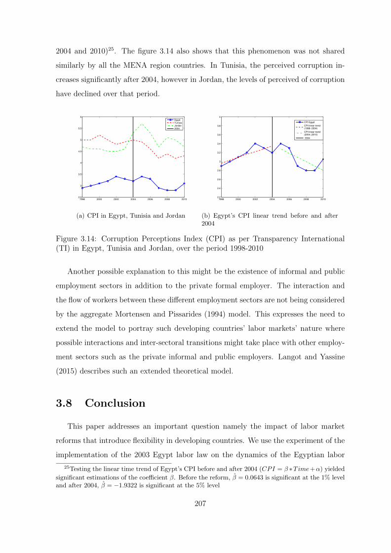
2004 and 2010)25. The figure 3.14 also shows that this phenomenon was not shared

similarly by all the MENA region countries. In Tunisia, the perceived corruption in-

creases significantly after 2004, however in Jordan, the levels of perceived of corruption

have declined over that period.

1998 2000 2002 2004 2006 2008 20102.5

3

3.5

4

4.5

5

5.5

6

Egypt

Tunisia

Jordan

2004

(a) CPI in Egypt, Tunisia and Jordan

1998 2000 2002 2004 2006 2008 20102.2

2.4

2.6

2.8

3

3.2

3.4

3.6

3.8

4

CPI Egypt

CPI linear trend(1998−2004)

CPI linear trend(2004−2010)

2004

(b) Egypt’s CPI linear trend before and after2004

Figure 3.14: Corruption Perceptions Index (CPI) as per Transparency International(TI) in Egypt, Tunisia and Jordan, over the period 1998-2010

Another possible explanation to this might be the existence of informal and public

employment sectors in addition to the private formal employer. The interaction and

the flow of workers between these different employment sectors are not being considered

by the aggregate Mortensen and Pissarides (1994) model. This expresses the need to

extend the model to portray such developing countries’ labor markets’ nature where

possible interactions and inter-sectoral transitions might take place with other employ-

ment sectors such as the private informal and public employers. Langot and Yassine

(2015) describes such an extended theoretical model.

3.8 Conclusion

This paper addresses an important question namely the impact of labor market

reforms that introduce flexibility in developing countries. We use the experiment of the

implementation of the 2003 Egypt labor law on the dynamics of the Egyptian labor

25Testing the linear time trend of Egypt’s CPI before and after 2004 (CPI = β ∗Time+α) yielded

significant estimations of the coefficient β. Before the reform, β = 0.0643 is significant at the 1% leveland after 2004, β = −1.9322 is significant at the 5% level

207

market, one of the most rigid markets at the end of the nineties. This reform came

to action in 2004, with the aim of enhancing the flexibility of the hiring and the firing

processes. Given the two components of unemployment, separation and job finding

rates, we measure the impact of the reform on each. Using constructed synthetic

retrospective panel datasets from the Egypt labor market panel surveys 2006 and 2012,

we are able to build a model to control for the recall and design bias such retrospective

data sets are likely to encounter. We therefore obtain the corrected trends of separation

and job finding rates over the period 1999-2011. These time series of workers’ flows,

that even official statistics fail to reproduce, are extremely important to be able to

understand the behavior of the dynamics of the Egyptian labor market necessary for

policy evaluation.

Our findings suggest that the new labor market reform increased significantly the

separation rates and had no significant impact on the job finding rates. Having decom-

posed the impact of the new law on both components and also by using counterfactual

experiments, we were able to conclude that the dynamics of the separation rates have

had an increasing dominant role in accounting for the changes in the unemployment

rate in Egypt especially after 2004. With increased separations and unchanged job

findings, the unemployment rates in the Egyptian labor market were shifted upwards

after 2004.

In the traditional Mortensen and Pissarides (1994) model, these empirical findings

can be explained only if the liberalization of the labor market is accompanied by a

capture of the new potential surpluses by corrupt agents. Indeed, in the Mortensen

and Pissarides (1994) model, the decrease in the firing costs allows the entrepreneurs to

take advantage of the facility to fire employees occupying obsolete jobs. But this decline

of taxes also gives incentive to create new jobs: this last phenomenon is not observed in

the data. Hence, we deduce that, expecting these increases in job surpluses, the corrupt

agents capture the value of these new opportunities: the costs due to corruption will

rise, and hence no hirings are encouraged. Knowing that the firms benefit from a larger

job surplus, a corrupt agent is more likely to charge extra costs (corruption costs) from

the firm than before the application of the reform. In addition to introducing hiring

subsidies to commit himself, the policymaker needs to make sure that corruption and

208

other set-up costs do not increase following such a reform. On the contrary, rules should

be set to fight against corruption to decrease such costs for the firms.

From a policy evaluation point of view, the law achieved only part of its mission,

where the firing (particularly to unemployment) process was largely facilitated. Yet it

has not been offset by a sufficiently increased and facilitated hiring process.

Extensions: The correction methodology proposed in this paper assumes a specific

parametric functional form of the estimated error terms. Further work is needed to

expand on the role of this functional form and to test to what extent the obtained

results depend on it. Moreover, since the three-state correction model is over-identified,

given nine free parameters and ten identifying restrictions, we shall be able to develop

tests of fit for the estimated error terms and hence the corrected transition matrices.

Computing the standard errors of the estimated parameters in the three state model,

would also enable us to test for their significance and construct confidence intervals for

the corrected flows and theoretical steady state stocks as has already been done for

the two state correction model. Calculating boot-strapped standard errors of both the

two-state and three-state models is also considered for future work.

209

References

Assaad, R., and C. Krafft (2013): “The Egypt labor market panel survey: intro-

ducing the 2012 round,” IZA Journal of Labor & Development, 2(1), 8.

Assaad, R., C. Krafft, and C. Yassine (2015): “Comparing Retrospective and

Panel Data Collection Methods to Assess Labor Market Dynamics,” .

Bassi, F., J. A. Hagenaars, M. A. Croon, and J. K. Vermunt (2000): “Es-

timating true changes when categorical panel data are affected by uncorrelated and

correlated classification errors an application to unemployment data,” Sociological

Methods & Research, 29(2), 230–268.

Blanchard, O. J., and P. Diamond (1990): “The cyclical behavior of the gross

flows of US workers,” Brookings Papers on Economic Activity, pp. 85–155.

Campos, N. F., and J. B. Nugent (2012): “The dynamics of the regulation of labor

in developing and developed countries since 1960,” Discussion paper, IZA Discussion

Paper Series.

Davis, S. J., and J. Haltiwanger (1990): “Gross job creation and destruction: Mi-

croeconomic evidence and macroeconomic implications,” in NBER Macroeconomics

Annual 1990, Volume 5, pp. 123–186. MIT Press.

(1992): “Gross job creation, gross job destruction and employment realloca-

tion,” Quarterly Journal of Economics, 107(3), 819–863.

De Nicola, F., and X. Gine (2014): “How accurate are recall data? Evidence from

coastal India,” Journal of Development Economics, 106, 52–65.

210

Hairault, J.-O., T. Le Barbanchon, and T. Sopraseuth (2013): “The cycli-

cality of the separation and job finding rates in France,” Discussion paper, Institute

for the Study of Labor, IZA.

Hodrick, R. J., and E. C. Prescott (1997): “Postwar US business cycles: an

empirical investigation,” Journal of Money, credit, and Banking, pp. 1–16.

Langot, F., and C. Yassine (2015): “Informal and Public Employment in developing

countries: Theory and application to the Egyptian case,” .

Lollivier, S., and V. Daniel (2002): “Erreurs de mesure et entrees-sorties de pau-

vrete (Documents de travail sur le site web),” .

Lucas, R. E. (1976): “Econometric policy evaluation: A critique,” in Carnegie-

Rochester conference series on public policy, vol. 1, pp. 19–46. Elsevier.

Magnac, T., and M. Visser (1999): “Transition models with measurement errors,”

Review of Economics and Statistics, 81(3), 466–474.

Mortensen, D. T., and C. A. Pissarides (1994): “Job creation and job destruction

in the theory of unemployment,” The review of economic studies, 61(3), 397–415.

Poterba, J. M., and L. H. Summers (1986): “Reporting errors and labor market

dynamics,” Econometrica: Journal of the Econometric Society, pp. 1319–1338.

(1995): “Unemployment benefits and labor market transitions: A multinomial

logit model with errors in classification,” The Review of Economics and Statistics,

pp. 207–216.

Rendtel, U., R. Langeheine, and R. Berntsen (1998): “The estimation of

poverty dynamics using different measurements of household income,” Review of

Income and Wealth, 44(1), 81–98.

Shimer, R. (2005): “The cyclical behavior of equilibrium unemployment and vacan-

cies,” American economic review, pp. 25–49.

(2012): “Reassessing the ins and outs of unemployment,” Review of Economic

Dynamics, 15(2), 127–148.

211

Veganzones-Varoudakis, M.-A., and C. Pissarides (2007): Labor markets and

economic growth in the MENA region, no. 278. Elsevier.

Wahba, J. (2009): “The impact of Labor market reforms on informality in Egypt:

Gender and work in the MENA region,” Discussion paper, The Population Council

Working Papers, 3. 0.

WorldBank (2014): “More Jobs, Better Jobs: A Priority for Egypt,” World Bank

Other Operational Studies, 19993.

Yassine, C. (2014): “Job Accession, Separation and Mobility in the Egyptian Labor

Market over the Past Decade,” Discussion paper, Economic Research Forum, Cairo.

Appendix

3.A Statistical Inference of the Correcting Param-

eters

3.A.1 Computing the Variance of Θ

In order to be able to test for the statistical significance of our correction method-

ology, we adopt the following steps to be able to calculate the standard deviations of

the estimated matrix of the unknown parameters Θ. We have

g(xT , Θ) = g(xT ,Θ0) +Dg(xT ,Θ0)(Θ−Θ0)

Dg(xT , Θ)′Wg(xT , Θ)︸ ︷︷ ︸=0 FOC

= Dg(xT , Θ)′Wg(xT ,Θ0) +Dg(xT , Θ)′WDg(xT ,Θ0)(Θ−Θ0)

where the left hand side of this last equation is equal to zero because it corresponds

the the FOC of the problem minΘ J :

Dg(xT , Θ)′Wg(xT , Θ) = 0 (3.37)

212

Hence, we deduce that

√T (Θ−Θ0) =

[Dg(xT , Θ)′WDg(xT ,Θ0)′

]−1

Dg(xT , Θ)′W√Tg(xT ,Θ0)

Given that Dg(xT , Θ) = −Dψ(ΘT ), we have

√T (Θ−Θ0) =

[Dψ(Θ)′WDψ(Θ0)′

]−1

Dψ(Θ)′W√T [ψT − ψ(ΘT )]

If, asymptotically,√T [ψT − ψ(ΘT )]→ N (0,W−1), then

√T (Θ−Θ0)→ N (0,ΣΘ)

with

ΣΘ =[Dψ(Θ)′WDψ(Θ0)′

]−1

Dψ(Θ)′WW−1WDψ(Θ)[Dψ(Θ)′WDψ(Θ0)

]−1

=[Dψ(Θ)′WDψ(Θ0)′

]−1

3.A.2 Corrected Flows and Steady-state Unemployment with

Confidence Intervals

The proposed correction methodology produces sugnificant estimated parameters.

In figure 3.15, we show the confidence intervals computed around the corrected time

deries of the separation and job finding rates, as well as the theoretical steady state

unemployment. The corrected flows are significantly different from the biased raw data

flows and the corrected steady state unemployment rate is significantly not different

from the empirical unemployment rate and can therefore be used as a proxy for the

unemployment rate in Egypt over the period 1999-2011 in our analysis.

213

1996 1998 2000 2002 2004 2006 2008 2010 20120

0.002

0.004

0.006

0.008

0.01

0.012

0.014

0.016Job separation rate

95% COnfidence IntervalsCorrected DataRaw Data

(a) Employment to unemployment separation

1996 1998 2000 2002 2004 2006 2008 2010 20120.05

0.1

0.15

0.2

0.25

0.3

0.35

0.4Job Finding rate

95% Confidence IntervalsCorrected DataRaw Data

(b) Unemployment to employment job finding

1996 1998 2000 2002 2004 2006 2008 2010 20120

0.02

0.04

0.06

0.08

0.1

0.12Unemployment rate

95%Confidence IntervalsSteady State U (data)Steady State U (corrected)Empirical unemp rate

(c) Unemployment rate

Figure 3.15: Job finding, separation and unemployment Rates in Egypt for maleworkers between 15 and 49 years of age, corrected for recall bias, two-state employ-ment/unemployment model

214

3.B OLS Regression Estimations

We report in the table 3.3 and 3.4 the ols regression estimations, of the two-state E-

U model, for the equations 3.38 and 3.39 (where ∆yt is used as an approximation for the

difference between the observed and the potential output), as well as the equations 3.40

and 3.41 (where yHPt is the detrended output series using the (Hodrick and Prescott,

1997) filter).

xt = α∆yt + b+ εt for x = f, s (3.38)

xt = α∆yt + b+ Iaγ + εt for x = f, s (3.39)

xt = αyHPt + b+ εt for x = f, s (3.40)

xt = αyHPt + b+ Iaγ + εt for x = f, s (3.41)

f f s sα -0.1436 -0.2577 -0.0122 -0.0430***b 0.1633*** 0.1629*** 0.0086*** 0.0085***γ 0.0108 0.0029***

Table 3.3: OLS regression results, a two-state E-U model

f f s sα 0.6980 0.6880 -0.0033 -0.0072b 0.1564*** 0.1532*** 0.0080*** 0.0067***γ 0.0062 0.0024***

Table 3.4: OLS regression results, a two-state E-U model (with HP filter)

In table 3.5, the three-state E-U-I ols regression estimations for the following equa-

tions 3.42, 3.43, 3.44 and 3.45 are illustrated.

xt = α∆yt + b+ εt for x = s, f,ΛEE,ΛEU ,ΛEI ,ΛUE,ΛUU ,ΛUI ,ΛIE,ΛIU ,ΛII (3.42)

xt = α∆yt + b+ Iaγ + εt for x = s, f,ΛEE,ΛEU ,ΛEI ,ΛUE,ΛUU ,ΛUI ,ΛIE,ΛIU ,ΛII(3.43)

xt = αyHPt + b+ εt for x = s, f,ΛEE,ΛEU ,ΛEI ,ΛUE,ΛUU ,ΛUI ,ΛIE,ΛIU ,ΛII (3.44)

xt = αyHPt + b+ Iaγ + εt for x = s, f,ΛEE,ΛEU ,ΛEI ,ΛUE,ΛUU ,ΛUI ,ΛIE,ΛIU ,ΛII(3.45)

215

f f s s

α -0.0570 0.2447 0.0020 -0.0302***b 0.1748*** 0.1727*** 0.0107*** 0.0107***γ -0.0029 0.0024***

ΛUE ΛUE ΛUU ΛUU ΛUI ΛUI

α 0.1259 0.0485 -0.2484 -0.3243 0.1224 0.2758b 0.1682*** 0.1679*** 0.8259*** 0.8257*** 0.0059 0.0064γ 0.0074 0.0072 -0.0146*

ΛEE ΛEE ΛEU ΛEU ΛEI ΛEI

α 0.0043 0.0190 -0.0167 -0.0487*** 0.0124 0.0296b 0.9813*** 0.9814*** 0.0085*** 0.0084*** 0.0102*** 0.0102***γ -0.0014 0.0030*** -0.0016*

ΛIE ΛIE ΛIU ΛIU ΛII ΛII

α -0.3293 -0.3744 -0.0148 -0.0029 0.3441 0.3774b 0.0998*** 0.0997*** 0.0313*** 0.0314*** 0.8688*** 0.8690***γ 0.0043 -0.0011 -0.0032

With HP filter f f s s

α 0.8679 0.8712 -0.0149 -0.0183*b 0.1828*** 0.1838*** 0.0106*** 0.0095***γ -0.0020 0.0021***

Table 3.5: OLS regression results, a three-state E-U-I model

216

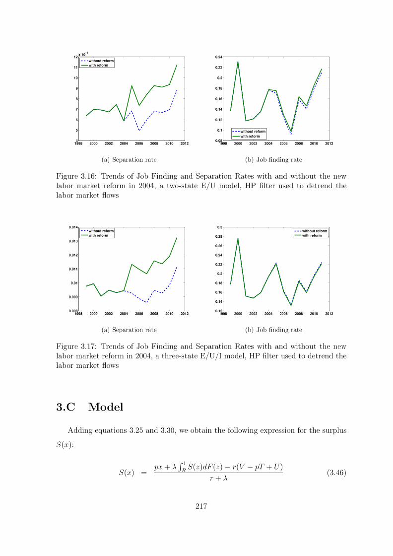
1998 2000 2002 2004 2006 2008 2010 20124

5

6

7

8

9

10

11

12x 10

−3

without reform

with reform

(a) Separation rate

1998 2000 2002 2004 2006 2008 2010 20120.08

0.1

0.12

0.14

0.16

0.18

0.2

0.22

0.24

without reform

with reform

(b) Job finding rate

Figure 3.16: Trends of Job Finding and Separation Rates with and without the newlabor market reform in 2004, a two-state E/U model, HP filter used to detrend thelabor market flows

1998 2000 2002 2004 2006 2008 2010 20120.008

0.009

0.01

0.011

0.012

0.013

0.014

without reform

with reform

(a) Separation rate

1998 2000 2002 2004 2006 2008 2010 20120.12

0.14

0.16

0.18

0.2

0.22

0.24

0.26

0.28

0.3

without reform

with reform

(b) Job finding rate

Figure 3.17: Trends of Job Finding and Separation Rates with and without the newlabor market reform in 2004, a three-state E/U/I model, HP filter used to detrend thelabor market flows

3.C Model

Adding equations 3.25 and 3.30, we obtain the following expression for the surplus

S(x):

S(x) =px+ λ

∫ 1

RS(z)dF (z)− r(V − pT + U)

r + λ(3.46)

217

Since S(R) = 0, we have λ∫ 1

RS(z)dF (z) = r(V − pT + U)− pR. This implies that

S(x) =p(x−R)

r + λ(3.47)

Now we go back to the S(R):

pR + λ∫ 1

RS(z)dF (z)− r(V − pT + U)

r + λ= 0

⇔ pR +λp

r + λ

∫ 1

R

(z −R)dF (z) = r(V − pT + U)

The reservation product, pR, plus the option value of continuing the match attributable

to the possibility that match product will increase in the future, the left-hand side,

equals the flow value of continuation to the pair, the right-hand side of the equation.

Using the sharing rule, we obtain the following :

(1− β)((W (x)− Ur + λ

) = β(J(x)− V + pT

r + λ) (3.48)

The option value cancels out, and so we are left with:

w(x) = (1− β)rU + β(px− r(V − pT ))

For the initial surplus, we add equations 3.27 and 3.29, and we use λ∫ 1

RS(z)dF (z) =

r(V − pT + U)− pR to obtain:

(r + λ)S0 = p(1−R)− (r + λ)p(C + T ) (3.49)

We also know that S(x) = p(x−R)r+λ

and for S0, x = 1, we can therefore write:

(r + λ)S0 = (r + λ)(S(x)− p(C + T ))

To obtain w0, we use the sharing rule:

β(J0 − pC − V ) = (1− β)(W0 − U)

218

The option value cancels and we finally obtain

w0 = (1− β)rU + β(p− r(V + U)− (r + λ)pC − λpT (3.50)

The free entry condition as mentioned previously is J0 = pcq(θ)

+ pC and so we can

re-write it as J0 − pC = pcq(θ)

. With V = 0, the sharing rule is J0 − pC = (1− β)S0 ⇒pc

1−β = q(θ)S0.

The value of an unemployed worker is therefore re-written as linear in θ as follows:

rU = b+ βθpc

1− β(3.51)

We substitute in the equations w0 and w(x), with V = 0:

w0 = (1− β)b+ βp(1 + cθ − (r + λ)C − λT )

w(x) = (1− β)b+ βp(θc+ x+ rT )

Subtituting the wage equations into the initial and continuing match value equations,

we obtain:

(r + λ)J0 = (1− β)p(1− x) + βp(r + λ)C + β(r + λ)pT − (r + λ)pT + (r + λ)(J(x) + pT )

Knowing that a job is destroyed when it’s no more profitable to the employer, we

can write J(R) + pT = 0. By evaluating equation 3.52 at R and since at free entry

J0 = pcq(θ)

+ pC, the job creation curve becomes:

(1− β)[(1−R)

r + λ− T − C] =

c

q(θ)(3.52)

219

Chapter 4

Informality, Public Employment

and Employment Protection:

Theory Using Evidence from Egypt1

4.1 Introduction

In chapter 1, it has been shown that the arab MENA countries in general, Egypt

in particular, are developing countries with rigid labor markets (low job finding and

separation rates). The public sector occupies a sizeable share of the jobs’ market and

has always been the main employer for workers in the region. With the democratic

transition as well as fiscal realities, the role of the public sector as the main employer

retreats allowing the development of the private sector and boosting the competitive-

ness of the labor market. However, the structure of the labor markets in developing

countries in general and in the MENA region in particular is much more complex. The

segmentation of these labor markets and the existence of an informal sector, due to the

lack of flexibility in the private formal sector 2, is almost a fact, where informality in

Egypt for instance counts up to approximately 40% of employment.

To date, very little is known about the internal dynamics of these labor markets.

The special features of the region’s labor markets make an understanding of the in-

1This chapter is based on work conducted jointly with Francois Langot2For descriptive statistics and a more detailed discussion of the labor market institutions in the

MENA region, paticularly Egypt and Jordan, see Chapter 1.

220

teraction between its different sectors crucial. The limited evidence to date indicates

that MENA labor markets suffer from high levels of inertia and rigidity, with rates of

job creation and destruction well below the levels observed in Europe and the United

States (Yassine (2014) (chapter 1, Langot and Yassine (2015) (chapter 3).

Since the flow approach to labor markets has become the basic toolbox to mod-

ern labor macroeconomics replacing the usual paradigm of supply and demand in a

frictionless environment, this paper proposes a dynamic job search model, that fits de-

veloping countries in general and MENA region countries in particular, where we take

into account the interaction between the public, formal private and informal private

sectors. A worker’s employment/non-employment choices are therefore based on the

comparisons between his/her expected job values in the current or all prospective jobs

i.e in any of the three employment sectors. If the theory omits any of these sectors, the

measures of the job turnovers, as well as transitions between sectors, can be biased.

This approach has as its central insight the assessement of the interactions between

the the three employment sectors namely public, private formal and private informal,

being crucial to explain the main labor market outcomes, one observes overtime. Limit-

ing the analysis, as previous traditional literature, to only an unsegmented or segmented

Private labor market might be insufficient or might fail to explain the inside story of

the underlying different transitions and the particular nature of the MENA region labor

markets. There have been recent attempts to include within the job search model an

informal sector (such as Albrecht, Navarro, and Vroman (2009), Meghir, Narita, and

Robin (2012), Bosch and Esteban-Pretel (2012), Charlot, Malherbet, and Ulus (2013,

2014) and Charlot, Malherbet, and Terra (2015)) or a public sector and an unseg-

mented private sector (Burdett (2012) , Bradley, Postel-Vinay, and Turon (2013)). In

this paper, we aim to add both an informal and a public sector to the conventional

Mortensen and Pissarides (1994) model.

In the previous chapter (Langot and Yassine, 2015), we adapted the aggregate

Mortensen and Pissarides (1994) to try to explain the impact of the implementation

of the 2003 Egypt labor law on the dynamics of the Egyptian labor market, one of the

most rigid markets at the end of the nineties. This reform came to action in 2004, with

the aim of enhancing the flexibility of the hiring and the firing processes. The empirical

221

findings suggest that the new labor market reform increased significantly the separation

rates and had no significant impact on the job finding rates. Theoretically, the intro-

duction of reduced firing taxes in a conventional Mortensen and Pissarides (1994), both

job creation and job destruction increase. The aggregate model can be adapted due to

the nature of a developing country where corruption exists and hence even if reducing

the firing tax, increases the surplus of the employer allowing him to create more jobs,

the corrupted agents knowing this can from their side increase the corruption set-up

cost they impose on the employers and hence nullify the positive effect of the new law

on job creation. However, another possible explanation to this might be the existence

of informal and public employment sectors in addition to the private formal employer.

Even though the policy is directed to the formal private sector, it surely affects the

interaction and the flow of workers between the different employment sectors. It is not

possible to explain using the conventional aggregate Mortensen and Pissarides (1994)

model the hidden inside story of these inter-sectoral flows underlying these outcomes.

In this paper, we therefore aim at testing for the robustness of these results by mod-

elling such developing countries’ labor markets’ nature where possible interactions and

inter-sectoral transitions might take place with other employment sectors such as the

private informal and public employers.

This paper therefore aims at the following main objectives:

1. Extend a theoretical job search equilibrium model a la Mortensen and Pissarides

(1994) showing the interaction between the 3 employment sectors namely (public,

formal and informal) and non-employment state.

2. Using qualitative analytics, calibrate the model and provide simulations for the

impact of the structural reforms following the democratic transitions of the MENA

region countries, particularly the Egypt Labor Law implemented in 2004.

3. Show supporting evidence from available data on flows in Egypt between the

employment sectors (private formal wage work, private informal wage work and

public sector wage work) and unemployment, before and after the 2004 reform.

In this paper, we choose to focus on exploring the effects of firing taxes and public

sector wage policies on job creation, job destruction, on-the-job search and employ-

222

ment. It is worth noting however that the model developed in this paper can be used

to explore the effect of changes of many other parameters such as subsidies, cost of

maintaining jobs, productivity shocks on labor market outcomes. For the purpose of

this chapter, we limit the analysis to firing taxes and public sector wage policies. The

model can therefore provide results and simulations that can provide main guidelines to

how the MENA region future employment policies, whether public or private, should

be directed in order to obtain the most efficient labor market outcomes during and

after the democratic transition period.

This paper should also be viewed as an attempt to explain to what extent the

Mortensen and Pissarides model is applicable to developing countries, such as Egypt,

where big shares of their employment lies in the informal 3 and public sectors. It

confirms the limitations of how the inside story of inter-sectoral transitions are not

displayed by the aggregate model. How can these interactions between sectors be

illuminating? First, the workers’ mobilities between sectors imply that their outside

options depend on opportunities in all sectors: when they bargain their wages in a

particular sector, they integrate their potential opportunities in other sectors. Hence,

if the formal sector becomes more profitable, the threat point of the employees in each

sector goes up, leading to wage pressures in the informal sector. If this last one does not

observe changes in its profitability, workers move to the formal sector, the most able

to support these high wages. The interaction between private (formal and informal)

sector and public sector is also interesting. Indeed, if the public sector provides high

wages, it is profitable for the employees to search on-the-job, in order to move to these

types of jobs. Hence, the public sector can act as an additional tax for the firms: they

pay an opening cost in order to hire workers, but during the duration of the contract,

some of these workers would choose to move for a better opportunity, in the public

sector. The model built in this paper also takes into consideration fiscal realities faced

by the public sector. It’s true that the public sector can increase its wages but given

its budgetary constraint, it is likely to decrease the rate at which it hires employees.

This could be done, as in Egypt for instance, by rationing public sector vacancies.

3The informal sector in this chapter, as throughout the entire thesis, is defined as employmentthat is not taxed or controlled by any form of government. The lack of a contract and social insuranceidentify informal wage workers in our dataset. See Chapter 1.

223

Our main findings suggest that introducing flexible employment protection rules,

modelled as reduced firing taxes, favors job creation and job destruction in the private

formal sector which is the main aim of the policy. It increases job separations in the

informal sector and decreases workers finding informal jobs. In general, introducing

flexibility into developing countries’ labor markets is important not only to promote

productivity growth along with economic growth, but also to scale down the difference

between formal and informal jobs. Such a reform causes a shift of employment from

informal jobs, which are very flexible by definition given that they are not controlled

by any institutional regulations, to formal work. The model developed in this paper

supports this. Indeed, it is shown that the liberalization of the labor market plays

against the informal employment by increasing the profitability of the formal jobs. But,

if at the same time, the wages offered by the public sector are increased, this would

create a crowding out effect: the new surpluses created by the labor market reform are

more than compensated by the new costs of worker mobility induced by the increase

in the attractiveness of the public sector. We show that this result is robust, even if

the introduction of reduced firing taxes decreases the proportion of on-the job search

towards the public sector of both workers in the formal and informal sectors. This paper

supports the view that since reducing firing taxes has been accompanied simultaneously

by a trending increase in the real wages of public sector workers 4, relatively higher

than the increase in the wages of private sector workers, formal and informal workers

are encouraged to search more on-the-job in the public sector: this tends to nullify

the positive effect on the private formal sector’s job creation, it even reduces it. The

net effect of the reform would therefore be an increase in the unemployment rates

since job separations in all cases are enhanced, but job findings remain unchanged or

even dampened. This therefore explains the empirical paradox of the Egyptian case

discussed in (Langot and Yassine, 2015), showing that following the liberalization of

the labor market, only job separations increase and job findings remain unchanged.

4Said (2015) shows that over the period 1998-2006, i.e. from a point in time before the reform toa point in time after, there has been a 40% increase in the median real monthly wages of governmentemployees, a 26% increase in the median real monthly wages of public enterprises’ employees and onlya 9% increase in the median real wage of the private sector.

224

4.2 A Model with Formal, Informal and Public Sec-

tors

4.2.1 Setting the Model

In this section, we propose an extension to the Mortensen and Pissarides (1994)

model to include the 3 sectors of the developing countries’ labor market; private formal

wage work (F), private informal wage work (I) and public sector (G). Our model is

founded, as the conventional Mortensen and Pissarides model, on the following concepts

for each of the private sectors, namely the formal (F ) and the informal (I):

1. A matching function that characterizes the search and recruiting process by which

a new job-worker matchis created in sector.

2. An idiosyncratic productivity shock captuing the reason for resource reallocation

across alternative activities in that specific sector.

3. An on-th-job search option allowing for an option that the job-worker match can

get destroyed as a worker transits to the public sector.

Given the above concepts, decisions about creation of new jobs, about recruiting

and search effort, and about the conditions that induce job-worker separations within

each sector can be formalized. Since our main focus is to study the job creation and de-

struction processes in the market, transitions between the formal and informal sectors

are not allowed in this model. These transitions are important to study the formaliza-

tion process of jobs and the way the quality of one’s job is improving, which is beyond

the study of this paper.

Job and worker matching in the private sector is viewed as a production process.

The functionmi(vi, u) represents the matching rate in sector i = F, I associated with

every possible vacancy in that sector and unemployment pair. Following Mortensen

and Pissarides (1994) and based on evidence from Petrongolo and Pissarides (2001),

constant returns is considered a convenient assumption, such that for i = F, I

mi(vi, u) = mi(1,u

vi) ≡ qi(θi) (4.1)

225

where θi = viu

, is the labor market tightness in sector i i.e. the ratio of vacancies in

that specific sector to the overall unemployment. These are endogenous variables and

are determined by the model.

In either the formal or the informal private sector, a vacant job is taken by a worker

at the rate qi(θi). The rate at which workers find jobs is θiqi(θi). Given that the

matching functions are assumed to be concave, homogenous and linear, qi(θi) decreases

in θi, while θiqi(θi) increases in θi.

Following the conventional model, the source of job-worker separations is job de-

struction attributable to an idisynchratic shock to match productivity (Mortensen and

Pissarides, 2001). Modelling this idea, the output of a job in sector i is the product

of two components pi, a common productivity of all jobs in a particular skill group

in sector i, and x, the idisyncratic component taking values on the unit interval and

arriving from time to time at the Poisson rate λi. Given an arrival of an idiosyncratic

shock, x is distributed according to the c.d.f. F (x). The sequence of shocks are iid.

In a specific sector, an existing match is destroyed if the idiosyncratic productivity

shock falls below an endogenous reservation threshold Ri specific to each sector. The

average rate of transition from employment in sector i to unemployment is therefore

λiF (Ri), which increases with the reservation threshold. Since certain workers, as has

been discussed in chapter 1, take the private sector (whether formal or informal) as

an intermediary till they get their appointment in the public sector, we allow for these

types of transitions among a productivity level (x) below a certain qualification thresh-

old (Qi). Offers from the public sector arrive at an exogenous poisson rate λiG, with

i = F, I depending on where the worker receing the offer is hired. In simple words,

when it’s a good/high productivity job, there is no interest to search for another and

when it’s a bad/low productivity job, it’s only an intermediate step till the public sec-

tor’s appointment arrives. In each of the private sectors, formal (F) and informal (I),

there are therefore 3 values: the initial value (0), when x is at its highest i.e. x = 1 ,

the no-search value (NS) when Qi < x ≤ 1 and the on-the-job search value (S), when

Ri ≤ x ≤ Qi.

226

0 Ri Qi 1

Match destroyed On-the-job search (S) No search (NS)

The Public sector is added as an a exogenous player. Wages, as well as the employ-

ment strategy are determined by the policy maker and should not be determined by

the Nash bargaining rule. The exogenous wages and number of individuals hired in the

public sector are however constrained by a government budget D. Workers within the

public sector are neither hit by productivity reallocation shocks nor get laid off. In all

sectors, workers retire at an exogenous rate δ.

The notations used in the model are close to the notations used in the conventional

literature on job search theory, just with the difference of being specific to the type of

private sector studied in our model. In general a firm with a profit opportunity in the

private sector, whether formal or informal opend a job vacancy for a worker with skill

indexed pi with i = F, I. The flow cost of recruiting in each sector is cipi. Applications

in each sector begin arriving at a hazard rate qi(θi(pi)), and one is received on average

1qi(θi(pi))

after the posting of the vacancy. As they meet, the worker and employer in

whichever sector start to bargain till they agree on an initial wage w0i (pi). Note that

the initial wage differs from one sector to the other and is dependent on the worker’s

skill. Job creation therefore takes place. Only in the formal sector, the firm is required

to pay a set-up cost pFC. This includes the cost of hiring in terms of legal formalities,

training and other forms of match specific investments. The informal sector being not

controlled by any form of government is assumed not incurr any of these costs. Wage

renegociation occurs with wage outcome wi(x, pi) prevailing on any continuing job, one

that generally reflects the new information x. As discussed above, if x falls below

some qualification level Qi(pi), on-the-job search towards the public sector becomes

an outside option for the workers. If x falls below some reservation level Ri(pi), job

destruction takes place. Only formal firms in that case pay a firing cost pFT . This

is an implicit firing tax imposed by employment protection regulations. Other policy

parameters are also considered in our model and only appear in the formal sector’s

equations. These include job creation or hiring subsidies denoted as pFH and payroll

taxes τ . Hiring subsidies are payments made to the employer when a worker is hired.

227

Finally, unemployed workers in the model enjoy imputed income during unemployment

b > 0. This income is independent of skill and represents the imputed value of leisure

to the worker, as well as all other forms of income that must be given up as the worker

moves from unemployment to employment. We formalize below the firm’ and workers’

behaviour in each sector.

4.2.2 Firms

Formal Firms

The initial value of an occupied job in the formal sector is given by the equation :

(r + δ)J0F (1) = pF − w0

F + τ + λF

∫ 1

RF

[maxJNSF (z), JSF (z) − J0

F (1)]dF (z)

+ λFFF (RF )[VF − pFT − J0F (1)] (4.2)

r represents the risk free interest rate. VF is the value of a vacancy in the formal private

sector. Since the idisyncratic component of a new job is x = 1 and due to the existence

of job creation costs pFC and policy parameters pFH and pFT , we define JF0 (1) as the

expected profit of a new match to the employer, given an initial formal sector wage w0F .

A continuing match has a specific productivity x. However, as explained in the

previous section, we define two intervals: (i) no search and (ii) on-the-job search.

QF is the skill threshold that determines whether workers are on the job-search or

not. If it’s a good (high productivity) job i.e x > QF , the workers will not be looking

for a job in the public sector i.e. no on-the-job search (NS). In that case, the worker

is paid a wage wNSF (x). The match can end in the future if a new match specific shock

z arrives and is less than some reservation threshold RF . The capital value of the job

to the employer JNSF (x) therefore solves the sollowing asset pricing equation for each

p:

(r + δ)JNSF (x) = pFx− wNSF (x) + τ + λF

∫ 1

RF

[maxJNSF (z), JSF (z) − JNSF (x)

]dF (z)

+ λFFF (RF )[VF − pFT − JNSF (x)] (4.3)

If it’s a bad (low-productivity) job x ≤ QF , the workers are looking for better

228

options in the public sector (on-the-job search S). This decreases the capital value of

the job to the employer. In the asset pricing equation, an outside option being the

transition of the worker from the formal sector to the public sector is added. This

becomes an additional possibility to why the match can end in the future. The worker

is paid a wage wSF (x) in that case.

(r + δ)JSF (x) = pFx− wSF (x) + τ + λF

∫ 1

RF

[maxJNSF (z), JSF (z) − JSF (x)

]dFF (z)

+ λFFF (RF )[VF − pFT − JSF (x)] + λFG(VF − JSF ) (4.4)

Given the definitions of the policy parameters described in the setting of the model,

the present value of an unfilled vacancy for a formal firm, VF , is:

rVF = −pF cF + qF (θF )(J0F (1)− pF (C −H)− VF ) (4.5)

Free entry requires that new vacancies are created until the capital value of holding

one is driven to zero i.e. VF = 0. The free entry condition for formal jobs can therefore

be formalized using the equation:

pF c

qF (θF )+ pF (C −H) = J0

F (1) (4.6)

The free entry condition therefore equates the cost of recruiting and hiring a worker to

the expected discounted future profit stream.

Informal Firms

The logic behind the behaviour of the informal firms is similar to that of the for-

mal firms except that any form of government regulation or policy parameter is being

excluded. It follows that, in the informal sector, there will neither be firing costs nor

setting up costs. The initial job value with an idiosyncratic productivity x = 1 in that

case would be exactly equal to the capital value of a job in a continuing match over the

no search interval i.e. if QI < x ≤ 1, formally J0I (1) = JNSI (1). QI is the skill threshold

that determines whether workers are on the job-search or not.

In the case of a high-productivity job i.e. x > QI , the only way the match can end

229

is in the future is if a new match with a specific showk z arrives and this shock being

less than than the reservation threshold Ri. With a wage wNSI (x), the expected profit

of the job to the employer is:

(r + δ)JNSI (x) = pIx− wNSI (x) + λI

∫ 1

RI

[maxJNSI (z), JSI (z) − JNSI (x)

]dFI(z)

+ λIFI(RI)[VI − JNSI (x)] (4.7)

When it’s a bad low-productivity job, i.e. x ≤ QI , on-the-job search towards the

public sector becomes an outside option and threatens the match to end in the future.

The capital value to an employer JSI (x) is therefore the solution of the asset-pricing

equation:

(r + δ)JSI (x) = pIx− wSI (x) +

∫ 1

RI

maxJNSI (z), JSI (z) − JSI (x)dFI(z)

+ λIFI(RI)(VI − JSI (x)) + λIG(VI − JSI (x)) (4.8)

In the informal sector there are no policy parameters,the value of a vacant job is

therefore:

rVI = −pIc+ qI(θI)JNSI (1) (4.9)

The free entry condition for informal firms therefore equates the cost of recruiting

and the anticipated profit of the match to the employer:

pIc

qI(θI)= JNSI (1) (4.10)

4.2.3 Workers

An analogous reasoning to that described in the behavior of the firms, is used to

analyse the workers’ behaviour. In general, an employed worker can be either employed

in the formal or the informal sector i = F, I respectively. According to the level of

productivity x, the worker decides whether to search on-the-job for better options in

the public sector or not.

230

The initial job value of a worker, W 0i (1), in sector i = F, I is when the idiosyncratic

component is at its highest value i.e. x = 1. This is expressed by the equation:

(r + δ)W 0i (1) = w0

i (1) + λi

∫ 1

Ri

[maxWNS

i (z),W Si (z) −W 0

i

]dFi(z)

+ λiF (Ri)(U −W 0i (1)) (4.11)

For a continuing match, as the specific productivity x is below the the on-the-job

search threshold of the sector, Qi, the worker will be searching for better options in the

public sector with an exogenous poisson rate of arrival of public sector offers λiG. The

rate at which the public sector hires workers is therefore specific to the sector i where

the worker is employed as he/she receives the offer. The worker’s value W Si (x) in that

case would solve the following asset pricing equation:

(r + δ)W Si (x) = wSi (x) + λi

∫ 1

Ri

[maxWNS

i (z),W Si (z) −W S

i (x)]dFi(z)

+ λiFi(Ri)(U −W Si (x)) + λiG(WG −W S

i (x)) (4.12)

If the specific productivity x exceeds the threshold Qi, the only outside option for

the worker becomes being unemployed. No on-the-job search takes place in that case.

The worker’s value over the no search interval is expressed by:

(r + δ)WNSi (x) = wNSi (x) + λi

∫ 1

Ri

[maxWNS

i (z),W Si (z) −WNS

i

]dFi(z)

+ λiFi(Ri)(U −WNSi (x)) (4.13)

Being unemployed in this economy, the individual receives an imputed income b > 0.

In the future, the unemployed can get hired by either of the three sectors, private formal,

private informal or public. The following bellman equation therefore solves for the value

of being unemployed, U :

(r + δ)U = b+ θF qF (W 0F (1)− U) + θIqI(W

0I (1)− U) + λUG(WG − U) (4.14)

By arriving to the public sector, the workers in our model are content with their

jobs. Evidence from the Egypt Labor Market Panel Survey in chapter 2 has shown that

231

transitions from the public sector to other sectors including the private sector (whether

formal or informal) and non-wage work are very few, sometimes nil. In the model, the

government employees are therefore assumed not to be searching for jobs in the private

sector. Moreover, transitions from employment to unemployment are very rare among

public sector workers and are therefore set to zero. The value of an employed worker

in the public sector is therefore, WG:

(r + δ)WG = wg (4.15)

In the formal sector, given a match product showk z, a firm decides to destroy a

job, whether on the on-the-job search or no search interval, if and only if the value of

holding it as a vacancy exceeds its value as a continuing job plus the firing costs pFT .

In other words, V jF > J jF (z) + pFT where j = NS, S. Similarly, a worker in the formal

sector prefers to stay unemployed if and only if U > Wi(z). Since, under the wage

rule, and as we will show below, J jF (z) and W jF (z) are increasing, separation occurs

when a new value of the shock arrives and falls below a reservation threshold RF . This

reservation productivity RF is defined as maxReF , RwF, where W jF (RwF ) = U and

J jF (ReF ) = VF − pFT . The separation rule in our case, a bilateral bargain, should be

jointly optimal in the sense that it maximizes the total wealth. The neccesary and

sufficient condition for this joint optimization is therefore RF = ReF = RwF implying

that J(RF ) +W (RF ) = VF − pFT + U .

Similarly, the same reasonong applies to come up with the reservation threshold and

the necessary and sufficient condition for the joint optimization in the informal sector.

The only difference is that no firing costs should be paid by the employer as jobs are

destroyed. It therefore follows that RI is defined as maxReI , RwI, where W jI (RwI) =

U and J jI (ReI) = VI , with j = S,NS. The necessary and sufficient condition for the

joint optimization would be RI = ReI = RwI leading to J(RI) +W (RI) = VI + U .

4.2.4 On-the-job Search

After deriving the value of the surplus in every sector, as shown in appendix 4.A, it

becomes possible to determine the threshold at which workers would decide to search

232

on-the-job or not.

Formal Sector

In the formal sector, the productivity threshold QF is defined when the surplus

obtained from a job with on-the-job search is equal to the surplus obtained from one

with no search, such that SNSF (QF ) = SSF (QF ). By doing so, one obtains

λFGSSF (QF ) = λFG[pFT + (WG − U)] (4.16)

which allows us to derive a unique value for QF , only if λFG > 0. If λFG = 0, the

threshold QF can not be defined.

Using equations 4.16 and 4.46, the expression for QF , the on-the-job threshold in

the formal sector, when λFG > 0 is :

QF = RF + (r + δ + λF + λFG)(T +WG − UpF

) (4.17)

Informal Sector

Similarly in the informal sector, the productivity threshold QI is defined when the

surplus obtained from an informal job with on-the-job search is equal to the surplus

obtained from one with no search, such that SNSI (QI) = SSI (QI). By doing so, one

obtains

λIGSSI (QI) = λIG(WG − U) (4.18)

As in the formal sector, the QI threshold is only defined if λIG > 0 and is conse-

quently expressed as follows:

QI = RI + (r + δ + λI + λIG)(WG − U

pI) (4.19)

233

4.2.5 Nash Bargaining and Wage Determination

As has been well established in the search equilibrium literature such as Diamond

(1981, 1982), Mortensen (1978, 1982), Pissarides, Layard, and Hellwig (1986), and

Pissarides (1990), the generalized aximatix Nash bilateral bargaining outcome with

threat point being the option to look for an alternative match partner is the baseline for

the wage determination. The wages are therefore bargained, with β being the worker’s

bargaining power and 1− β the employer’s, and setting Vi = 0 (i = F, I) according to

the free-entry condition. By using the definitions and expressions of surpluses derived

in appendix 4.A, we are able to build up the first order conditions of the standard

wage optimization problem for each sector i = F, I, during the absence and presence

of on-the-job search.

For the initial wage of a job in the formal sector:

β(J0F (1)− VF − pF (C −H)) = 1− β(W 0

F (1)− U) (4.20)

For a continuing job in the formal sector with x ≤ QF

β(JSF (x)− VF − pFT ) = 1− β(W SF (x)− U) (4.21)

For a continuing job in the formal sector with x > QF

β(JNSF (x)− VF − pFT ) = 1− β(WNSF (x)− U) (4.22)

Recalling that the initial wage in the informal sector is the same as the wage of a

no-search job when x = 1, i.e. w0I (1) = wNSI (1), the first order condition for a job in

the informal sector with x > QI

β(JNSI (x)− VI) = 1− β(WNSI (x)− U) (4.23)

For a job in the informal sector with x ≤ QI

β(JSI (x)− VI) = 1− β(W SI (x)− U) (4.24)

234

Using the free entry conditions for the formal and informal sectors pF cqF (θF )

+pF (C−H) =

J0F (1) and pIc

qI(θI)= JNSI (1) respectively, we can re-write (W 0

F (1) − U) = β1−β

pF cqF (θF )

and

(WNSI (1)− U) = β

1−βpIcqI(θI)

. This implies :

(r + δ)U = b+β

1− β(cF θFpF + cIθIpI) + λUG(WG − U) (4.25)

Using the public sector worker’s value function (r + δ)WG = wg:

WG − U =wG − b− βc

1−β (θFpF + θIpI)

r + δ + λUG(4.26)

Plugging WG − U into the value equation of the unemployed, we obtain:

(r + δ)U =r + δ

r + δ + λUG(b+

βc

1− β(θFpF + θIpI)) +

λUGr + δ + λUG

wG (4.27)

Introducing these results in the wage equations, we obtain the expressions for the intial

wages and wages in continuing jobs in both the formal and informal sectors.

• Formal Sector: The initial wage expression in the formal sector therefore be-

comes:

w0F (1) = β(pF + τ − (r + δ + λF )pF (C −H)− λFpFT +

r + δ

r + δ + λUGc(θFpF + θIpI))

+ (1− β)[r + δ

r + δ + λUGb+

λUGr + δ + λUG

wG]

For the wages of jobs occupied by workers who are looking out for outside options

in the public sector, i.e. x ≤ QF

wSF (x) = β[pFx+ τ − (r + δ + λFG)pFT +r + δ + λFGr + δ + λUG

c(θFpF + θIpI)]

+ (1− β)[r + δ + λFGr + δ + λUG

b+λUG − λFGr + δ + λUG

wG]

For a continuing match, when workers are not searching on the job, x > QF , we

235

have:

wNSF (x) = β(pFx+ τ − (r + δ)pFT +r + δ

r + δ + λUGc(θFpF + θIpI))

+ (1− β)[r + δ

r + δ + λUGb+

λUGr + δ + λUG

wG]

As in the conventional Mortensen and Pissarides model, the wages of the formal

sector depend on the policy parameters. By introducing the informal sector in the

model, these wages not only depend on the labor market tightness in the formal

segment of the market, but also on the labor market tightness in the informal

sector. As the tightness θi increases in any of the sectors, the net share of match

product obtained by the employer increases. Adding the public sector increases

the bargained share by the worker, whether at the start of the job since now the

outside option is not only being unemployed and receiving an imputed income

b. It is now possible for an unemployed worker to get hired by the public sector

and this therefore adds to the his net share of the bargained wage. Moreover,

the on-the-job search possibility acts as a liability to the employer. It therefore

strengthens the worker’s hand in the wage bargain.

• Informal Sector: Similarly in the informal sector, the wages depend on the

labor market tightness in both segments of the private sector, θI and θF . Since

the informal sector is any form of employment that is not regulated by the gov-

ernment, the wages in this sector do not depend by any means of the policy

parameters. The outside option of getting hired by the public sector, however,

strengthens the worker’s bargain and acts as a tax or liability to the employer.

The informal wage in a continuing match in the informal sector, when workers

are searching on-the-job, i.e. x ≤ QI , becomes:

wNSI (x) = β[pIx+r + δ

r + δ + λUGc(θFpF + θIpI)]

+ (1− β)[r + δ

r + δ + λUGb+

λUGr + δ + λUG

wG] (4.28)

236

When, there is no on-the-job search, x > QI , the wage equation is defined as:

wSI (x) = β[pIx+r + δ + λiGr + δ + λUG

c(θFpF + θIpI)]

+ (1− β)[r + δ + λiGr + δ + λUG

b+λUG − λiGr + δ + λUG

wG]

4.2.6 Equilibrium

It remains to substitute the wage equations we derived in the previous section

into the asset value equations, the job creation, job destruction and on-the-job search

conditions, in order to derive the overall market equilibrium. This equilibrium would

be characterized by the labor market tightness in each segment of the private sector,

θF and θI , the reservation productivity threshold for each sector, RF and RI , and the

on-the-job search threshold in each sector QF and QI .

Job Creation Condition

Recalling the free-entry conditoin in the formal sector, presented in equation 4.6

and by using S0F (1) = SNSF (1) − pF (C − H + T ), the job creation condition for the

formal sector is can be deduced as follows:

pF cFqF (θF )

= (1− β)[pF (1−RF )− λFGpFT − λFG(WG − U)

r + δ + λF− pF (C −H + T )]

(4.29)

For the informal sector, the free-entry condition in equation 4.10 allows us to write the

informal sector’s job creation condition as follows:

pIcIqI(θI)

= (1− β)[pI(1−RI)− λIG(WG − U)

r + δ + λI] (4.30)

Job Destruction Condition

In the formal sector, we derive the job destruction condition by the equation:

pFRF = (r + δ)U − τ − λF∫ 1

RF

SF (z)dFF (z)− (r + δ + λFG)pFT − λFG(WG − U)(4.31)

237

while for the informal sector, we obtain

pIRI = (r + δ)U − λI∫ 1

RI

SI(z)dFI(z)− λIG(WG − U)

The job destruction conditions suggest that the at the worst possible surplus,

whether for the formal or informal sector, the reservation productivity does not only

depend on the possible gains from the match in the sector itself. It depends as well on

the potential gains one could have from passing on eventually to a job in the public

sector after being for a while in the formal or the informal sector. A worker might

prefer having a low salary in the private sector i.e. a low reservation productivity Ri,

whether formal or informal i = F, I, knowing that eventually he/she can access the

public sector via this job.

On-the-job search Condition

As have been previously derived, the on-the job search condition in the formal sector

is re-written as:

pFQF = pFRF + (r + δ + λF + λFG)(pFT +WG − U) (4.32)

and for the informal sector as:

pIQI = pIRI + (r + δ + λI + λIG)(WG − U) (4.33)

All the above labor market conditions use the folowing expressions which are func-

tions of the endogenous θi, Ri and Qi, i = F, I, to be determined by solving the model:

∫ 1

RF

SF (z)dFF (z) =pF

r + δ + λF + λFG

−(QF −RF )(1− FF (QF )) +

∫ QF

RF

[1− FF (x)]dx

pF

r + δ + λF

(QF −RF )(1− FF (QF )) +

∫ 1

QF

[1− FF (x)]dx

+λFGpFT − λFG(WG − U)

r + δ + λF(1− FF (QF ))

238

∫ 1

RI

SI(z)dFI(z) =pI

r + δ + λI + λIG

−(QI −RI)(1− FI(QI)) +

∫ QI

RI

[1− FI(x)]dx

pI

r + δ + λI

(QI −RI)(1− FI(QI)) +

∫ 1

QI

[1− FI(x)]dx

+λIG(1− FI(Q1))

r + δ + λI(WG − U)

(r + δ)U =r + δ

r + δ + λUG(b+

βc

1− β(θFpF + θIpI)) +

λUGr + δ + λUG

wG

WG − U =wG − b− βc

1−β (θFpF + θIpI)

r + δ + λUG

4.3 Steady-state Stocks

The entire Population of the eocnomy, Pop, is sub-divided into four sub-populations:

the unemployed u, public sector employees nG, formal private sector wage workers nF

and informal private sector wage workers nI .

1 = nF + nI + nG + u (Pop) (4.34)

Since the model is assumed to be in steady-state, for each sub-population, inflows

are equal to the outflows. This can be formalized by the equations

δnG = λUGu+ λFGnF + λIGnI (NG) (4.35)

fFu = λFFF (RF )nF + λFGnF (NF ) (4.36)

fIu = λIFI(RI)nI + λIGnI (NI) (4.37)

Given the above relationship, the number of workers hired in the public sector is given

239

by the equation:

nG =λUG

δ + λUG+λFG − λUGδ + λUG

fFλFFF (RF ) + λFG

u+λIG − λUGδ + λUG

fIλIFI(RI) + λIG

u

(4.38)

It’s important to note at this point that due to fiscal realities, even though the hiring

and wage policies in the public sector, they are constrained by the government’s budget.

This is defined as D such that

D = nG(λUG, λFG, λIG)× wG (4.39)

Finally the steady-state unemployment rate is obtained.

u =δ(λIFI(RI) + λIG)(λFFF (RF ) + λFG) (λIFI(RI) + λIG)(λFG + δ)fF + (λFFF (RF ) + λFG)(λIG + δ)fI

+(λIFI(RI) + λIG)(λFFF (RF ) + λFG)(λUG + δ)

(4.40)

4.4 A Numerical Analysis of the Model

One of the main aims of this paper is to explain how the labor market equilibrium,

particularly job creations and job destructions, in developing countries, such as Egypt,

react as flexible employment protection is introduced in their markets. Liberalizing

the labor market is modelled theoretically by reduced firing taxes T . Although the

model developped in this paper can be used to analyse the impact of changing many

parameters such as hiring subsidies, cost of maintaining jobs, productivity shocks on

labor market outcomes. We choose to focus on the Egyptian case and the introduction

of the 2004 Labor Law, to try to explain the paradoxal empirical result obtained in

Langot and Yassine (2015) (chapter 3). In the latter chapter, identifying the reform as

a structural break in the job findings and separations time series, it has been shown

that as the firing taxes were reduced, only separations increased significantly. Job

creations remain unchanged. Moreover, evidence from Said (2015), pointed out, during

the period 1998-2006, i.e. during the time period where the reform came into action,

a relatively higher increase in the median real wages of public sector employees. Since

240

the public sector can not continue hiring employees at increased salaries due to budget

constraints, there has been a decline in the public sector hiring over the same period. In

this section, we therefore focus on exploring the effects of firing taxes and public sector

wage policies on job creation, job destruction, on-the-job search and employment.

We present computed solutions to the model that provide some numerical feel for

its policy implications. Parsimonious functional forms are assumed. The parameters

are set at reasonable values and are chosen to match unemployment spell durations and

incidences typically experienced by the Egyptian workers in the different sectors. The

next section provide empirical evidence on the labor market transition probabilities in

the Egyptian labor market over the period 1999-2011 (i.e before and after the reform).

Chapters 1 and 2 also provide detailed descriptive statistics in the labor market tran-

sition probabilities, sectors’ shares and unemployment rates obtained from the Egypt

Labor Market Panel Survey, fielded in 2012. Some of these descriptive statistics provide

guidelines in our numerical analysis to choose the baseline parameters.

Following (Mortensen and Pissarides, 2001), the matching function of sector i = F, I

is log-linear. Formally,

qi(θi) = θ−ηii

where without loss of generality the scale parameter is normalized to one (this assump-

tion simply determines the units in which vi, and so θi, are measured) and ηi is the

constant elasticity of each sector’s matching function with respect to unemployment.

The distribution of the idiosyncratic shock to match productivity is uniform over the

interval [γi, 1]. We therefore have:

Fi(x) =x− γi1− γi

The baseline parameter used for the policy cases under study are presented in Table

4.1. This table also justifies the choice of the value of the baseline parameters. This

could be chosen following previous search equilibrium literature, inspired by the data

or modified to fit results that match the economy in question. The normalized skill

parameter value pF = 1 is interpreted as the initial match product of a worker of

241

average ability in the formal sector. The skill parameter of a worker in the informal

sector is assumed to be lower, pI = .9. The analysis considers only the case of an

efficient equilibrium solution to the model, where β = η

The Egypt Labor Law, implemented in 2004, introduced lower levels of employment

protection in the Egyptian Labor market. Theoretically, this is modelled as a reduction

in the firing tax T . In Figure 4.1, we show the impact of decreasing the firing taxes on

the steady-state labor market outcomes, assuming that all other baseline parameters

have remained unchanged after the reform. The blue line in the steady state outcomes

subpanel (a) represent the reference economy obtained using the baseline parameters

and T = 2. We note that both separations in the formal and informal sectors increase,

since both RF and RI (the reservation productivity levels) shift upwards after the re-

form. The increase in separations is proportional in magnitude to the decrease in the

firing taxes, i.e the larger the reduction in Taxes, the larger the increase in job destruc-

tion. For the job creations, the story is different. As suggested by the conventional

Mortensen and Pissarides (1994) model, the decrease in the firing tax leads to an in-

crease in the job creations of the formal sector. This is the direct effect, corresponding

to the shift of the job creation curve in the plane (labor market tightness, reservation

productivity) which always dominates the reduction of the employment duration im-

plied by the increase in the separation (the shift of the job destruction curve in the plane

(labor market tightness, reservation productivity)). Extending the model to include the

informal sector, shows that such a reform decreases the job creations in the informal

sector: the new opportunities in the formal sector push up the real wages in all sectors,

and hence reduce the hiring in the sector where this increase of labor costs is not over-

compensated by a reduction of tax (the firing taxes in the formal sector). The reform,

therefore scales down the difference between the formal and informal sector by shifting

employment favoring the formal sector. Moreover, our simulations show that decreas-

ing firing taxes reduces substantially the on-the-job search of private formal workers

towards the public sector jobs. It is shown that if the decrease in T is huge,the share

of workers on-the-job search in the formal sector, described by the difference between

QF and RF , might be very small. This is mainly driven by combined effect of the small

decrease in the on-the-job search threshold QF along with a substantial increase in the

242

reservation productivity RF for a given dT . In the informal sector, on-the job search

towards the public sector almost remains unchanged or slightly decreases, following a

relatively small increase in the reservation productivity RI and almost no change in the

on-the-job search threshold QI . Figure 4.1 also shows following the reduction in firing

taxes, overall steady-state unemployment shifts upwards.

Parameters Benchmark Reason for setting this value

Output per worker in Formal pF 1 Previous LiteratureOutput per worker in Informal pI 0.9 Lower than the Formal SectorWorker Bargaining power β 0.5 Previous LiteratureInterest rate r 0.09 Average interest rate in EgyptReallocation Shock (Formal) λF 0.01 very low to reflect low separationsReallocation Shock (Informal) λI 0.02 Separations are more frequent than in the Formal SectorTransition from Formal to Public λFG 0.012 Transition rate from ELMPS 2012 DataTransition from Formal to Public λIG 0.009 Transition rate from ELMPS 2012 DataTransition from unemployment to Public λUG 0.015 Transition rate from ELMPS 2012 DataFixed cost of maintaining a formal job cF 0.3 Previous LiteratureFixed cost of maintaining an informal job cI 0.3 Previous LiteratureCost of Setting up a costC 0.3 Previous LiteratureHiring Subsidy H 0 Does not existDuration Elasticity (Formal Sector) ηF 0.5 To obtain an efficient equilibrium solutionDuration Elasticity (Informal Sector) ηI 0.5 To obtain an efficient equilibrium solutionLower productivity shock support (Formal) γF 0.1 Adjusted to obtain reasonable results

and typically lower than developed countries in previous literatureLower productivity shock support (Informal) γI 0.08 Lower than the Formal sectorValue of Leisure b 0.3 Previous LiteratureMatching Efficiency (Formal) qF 0.07 differentiated from the informal sectorMatching Efficiency (Informal) qI 0.1 Assumed to be easier to match worker-jobPublic Sector Wage wG 0.8 Adjusted to obtain reasonable resultspayroll tax τ 0.2 Typical payroll taxFiring Tax T 2 Adjusted to obtain reasonable resultsRetirement rate δ 0.007 Public Sector separations in the data

Table 4.1: Baseline parameters

243

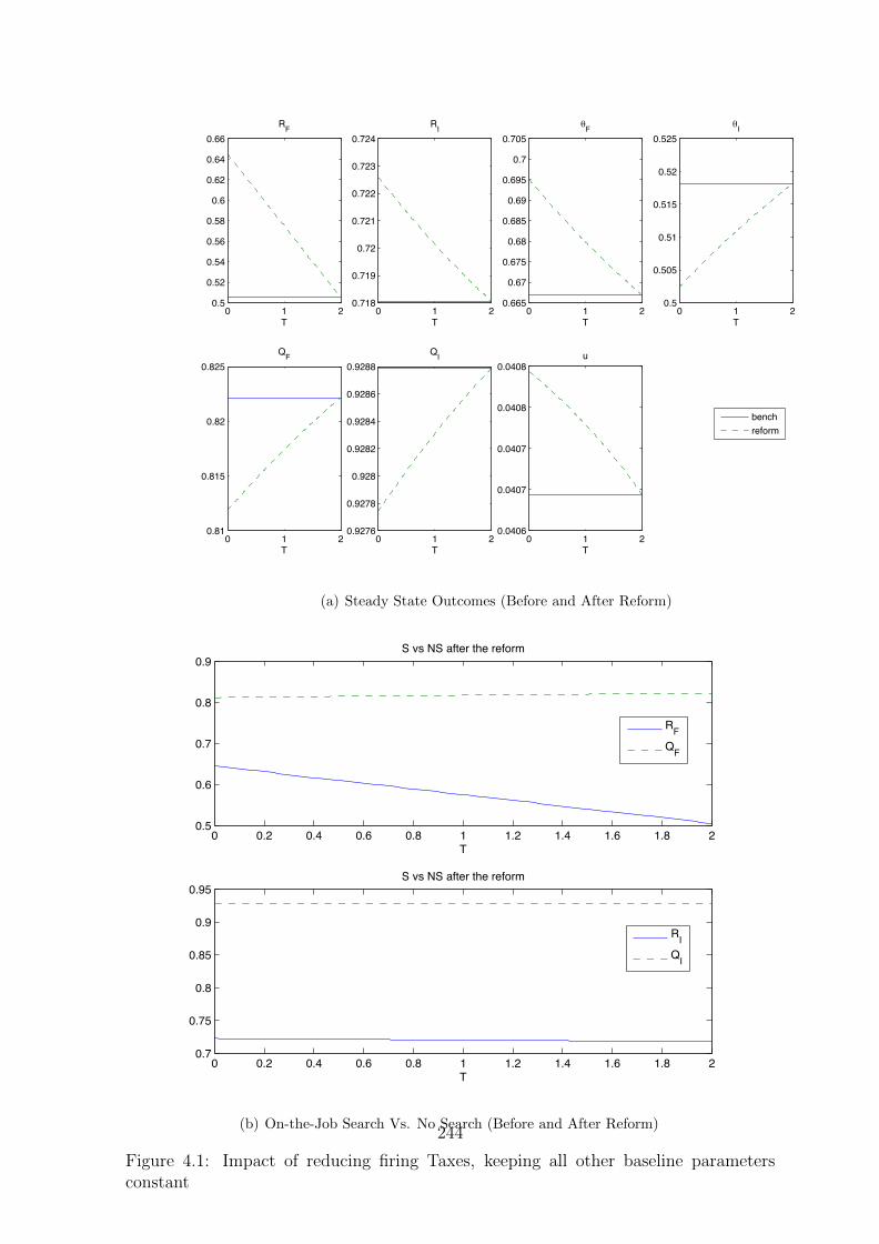
0 1 20.5

0.52

0.54

0.56

0.58

0.6

0.62

0.64

0.66

T

RF

benchreform

0 1 20.718

0.719

0.72

0.721

0.722

0.723

0.724RI

T0 1 2

0.665

0.67

0.675

0.68

0.685

0.69

0.695

0.7

0.705θF

T0 1 2

0.5

0.505

0.51

0.515

0.52

0.525θI

T

0 1 20.81

0.815

0.82

0.825QF

T0 1 2

0.9276

0.9278

0.928

0.9282

0.9284

0.9286

0.9288QI

T0 1 2

0.0406

0.0407

0.0407

0.0408

0.0408u

T

(a) Steady State Outcomes (Before and After Reform)

0 0.2 0.4 0.6 0.8 1 1.2 1.4 1.6 1.8 20.5

0.6

0.7

0.8

0.9

T

S vs NS after the reform

RFQF

0 0.2 0.4 0.6 0.8 1 1.2 1.4 1.6 1.8 20.7

0.75

0.8

0.85

0.9

0.95

T

S vs NS after the reform

RIQI

(b) On-the-Job Search Vs. No Search (Before and After Reform)

Figure 4.1: Impact of reducing firing Taxes, keeping all other baseline parametersconstant

244

Evidence from Said (2015) has shown, however, that during the period 1998-2006,

i.e. during the time period where the reform came into action, there has been a rela-

tively higher increase in the median real wages of public sector employees. Said (2015)

shows that there has been a 40% increase in the median real monthly wages of gov-

ernment employees and a 26% increase in the median real monthly wages of public

firms’ employees, as opposed to only a 9% increase in the median real wage of the

private sector. The government is faced however by fiscal realities, in other words it

is constrained by a budget, denoted by D in the model. Even if the wages increase,

the government will have to decrease its hiring rate. In reality, this could be done via

rationing public sector jobs, as in Egypt. To be able to calibrate this theoretically, we

fix a budget constraint, given the initial public sector wage w0G and the initial share

of public sector employees n0G, D0 = n0

G(λ0FG, λ

0IG, λ

0UG) × w0

G. As the public sector

wage increases and the budget remains unchanged, the resulting nG(λFG, λIG, λUG) is

deduced assuming the functional form :

λiG =λ0iG

(1 + exp(a× wG)− exp(a× w0G))

(4.41)

where λiG is the new public sector hiring rate from i = F, I, U , wG is the public sector

wage after the increase and a is a parameter that is determined endogenously as the

model is solved given D0 and the new nG.

In figure 4.2, we show how the steady-state labor market outcomes vary in response

to only a variation in the public sector wages. The blue line in subpanel (a) there-

fore represents the reference economy obtained using the baseline parameters. We

choose however a lower level of firing tax T = 1, reflecting that the market has already

been liberalized by the reform. Interestingly, the increase in public sector wages show

opposite effects to the decrease in firing costs on the reservation productivity levels

of both sectors RF and RI . These effects are non-linear given that the increase in

wages is accompanied by a non-linear decrease in the public sector hiring rate from all

sectors. As has been explained in the theoretical model, as the public sector jobs be-

come more attractive, the reservation productivities RF and RI are pushed downwards.

Consequently, increasing the public sector’s wages while keeping all other parameters

245

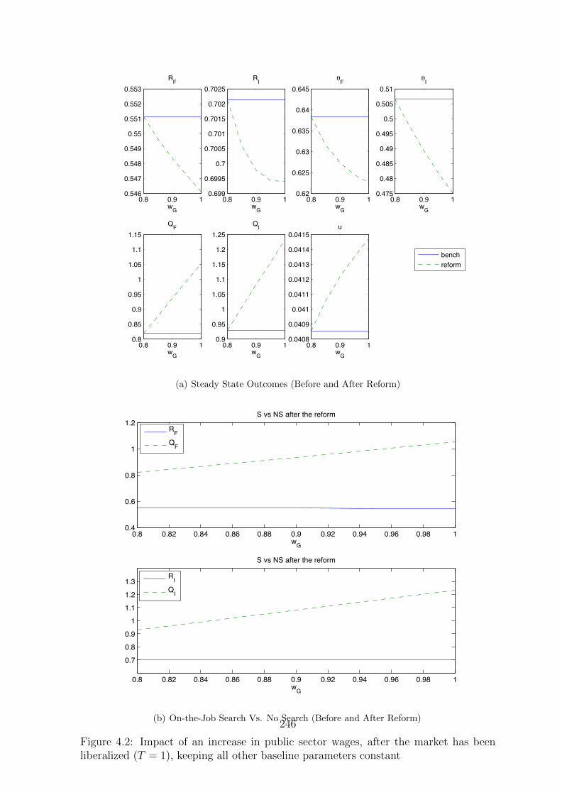
0.8 0.9 10.546

0.547

0.548

0.549

0.55

0.551

0.552

0.553

wG

RF

benchreform

0.8 0.9 10.699

0.6995

0.7

0.7005

0.701

0.7015

0.702

0.7025RI

wG

0.8 0.9 10.62

0.625

0.63

0.635

0.64

0.645θF

wG

0.8 0.9 10.475

0.48

0.485

0.49

0.495

0.5

0.505

0.51θI

wG

0.8 0.9 10.8

0.85

0.9

0.95

1

1.05

1.1

1.15QF

wG

0.8 0.9 10.9

0.95

1

1.05

1.1

1.15

1.2

1.25QI

wG

0.8 0.9 10.0408

0.0409

0.041

0.0411

0.0412

0.0413

0.0414

0.0415u

wG

(a) Steady State Outcomes (Before and After Reform)

0.8 0.82 0.84 0.86 0.88 0.9 0.92 0.94 0.96 0.98 10.4

0.6

0.8

1

1.2

wG

S vs NS after the reform

RFQF

0.8 0.82 0.84 0.86 0.88 0.9 0.92 0.94 0.96 0.98 1

0.70.80.9

11.11.21.3

wG

S vs NS after the reform

RIQI

(b) On-the-Job Search Vs. No Search (Before and After Reform)

Figure 4.2: Impact of an increase in public sector wages, after the market has beenliberalized (T = 1), keeping all other baseline parameters constant

246

constant, separations are dampened in both sectors. It is interesting for workers to stay

temporarily in these private sector jobs knowing that eventually there are potentials to

move to the public sector. It is worth noting that it might be possible however, that

even if the public sector wages increase, in case the hiring rate encounters a substan-

tial relative decrease, in other words λiG is very elastic, there exists less potential to

move to public sector jobs. In that case the reservation productivities might on the

contrary increase or remain unchanged. Figure 4.3 shows an example to this possible

phenomenon. This shows the response of the steady-state labor market outcomes in

response to only a variation in the public sector wages at a higher level of firing tax

T = 2 i.e. a more rigid formal sector.

Moreover, following the rise of wG, it becomes more attractive for all workers to

search for better options and potential jobs in the Public sector. Job creations in both

private formal and informal sectors are discouraged. Again this decrease is non-linear

depending on the way job finding rate in the public sector decreases. Generally, by

raising its attractiveness, the public sector reduces the expected employment duration

of each job, and hence the expected surplus. This implies that θF and θI decrease.

On-the-job search in both sectors also increases, given that workers can now gain more

with higher wages in the public sector.

That being said, we can conclude our analysis by studying the simultaneous changes

of firing taxes and public wages, and precisely by a decrease in the firing taxes, accom-

panied by an increase in the public sector wages. In table 4.4, we detail the impact of

the change in each of these parameters on the model’s equilibrium, trying to sum up

the expected combined net effect on the labor market outcomes. Figures 4.4 and 4.5

show the analytical results using a three-dimensional display of the impact of variations

in both firing taxes and public sector wages simultaneously on steady-state outcomes.

On-the job search towards the public sector is encouraged in both sectors the formal

and informal, thanks to the rise in wG. This is obvious in figure 4.4. The positive

effects on job creations resulting from the liberalization of the labor market, following

the reform, becomes nullified or sometimes worsened (where creations are dampened)

by an increase in the public sector wage.

Overall for the formal sector’s separtions, i.e. RF (Figure 4.5), there has been

247

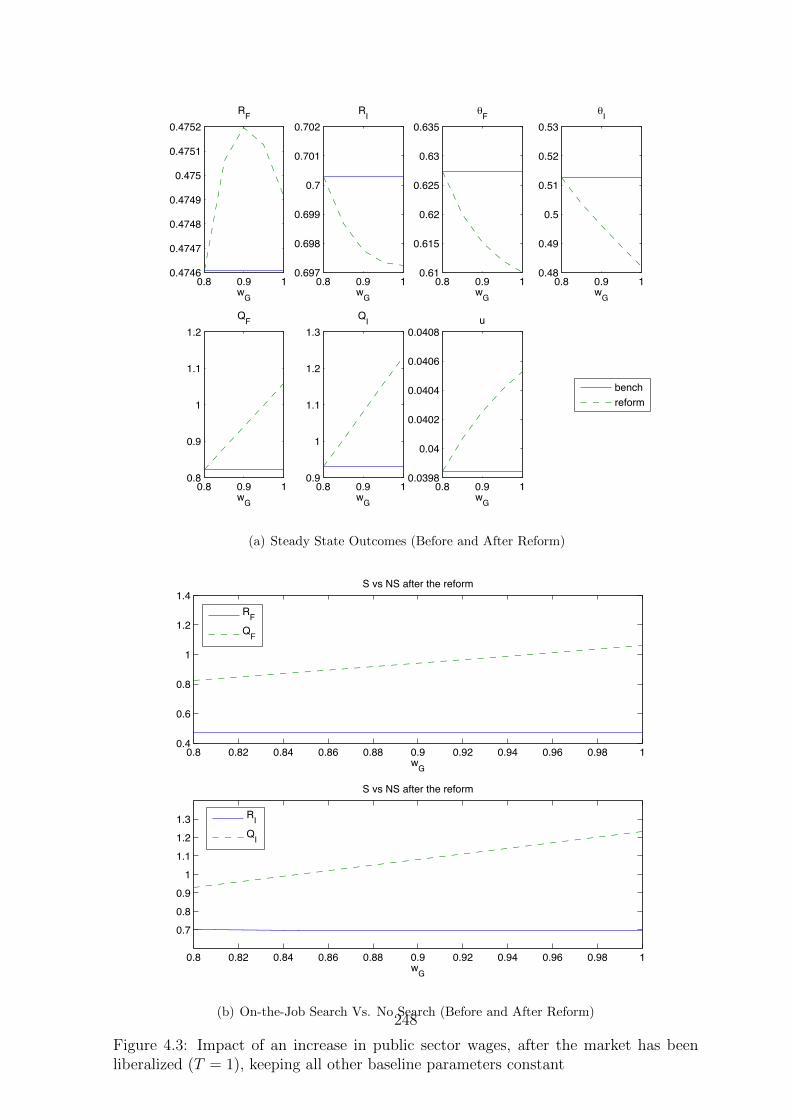
0.8 0.9 10.4746

0.4747

0.4748

0.4749

0.475

0.4751

0.4752

wG

RF

benchreform

0.8 0.9 10.697

0.698

0.699

0.7

0.701

0.702RI

wG

0.8 0.9 10.61

0.615

0.62

0.625

0.63

0.635θF

wG

0.8 0.9 10.48

0.49

0.5

0.51

0.52

0.53θI

wG

0.8 0.9 10.8

0.9

1

1.1

1.2QF

wG

0.8 0.9 10.9

1

1.1

1.2

1.3QI

wG

0.8 0.9 10.0398

0.04

0.0402

0.0404

0.0406

0.0408u

wG

(a) Steady State Outcomes (Before and After Reform)

0.8 0.82 0.84 0.86 0.88 0.9 0.92 0.94 0.96 0.98 10.4

0.6

0.8

1

1.2

1.4

wG

S vs NS after the reform

RFQF

0.8 0.82 0.84 0.86 0.88 0.9 0.92 0.94 0.96 0.98 1

0.70.80.9

11.11.21.3

wG

S vs NS after the reform

RIQI

(b) On-the-Job Search Vs. No Search (Before and After Reform)

Figure 4.3: Impact of an increase in public sector wages, after the market has beenliberalized (T = 1), keeping all other baseline parameters constant

248

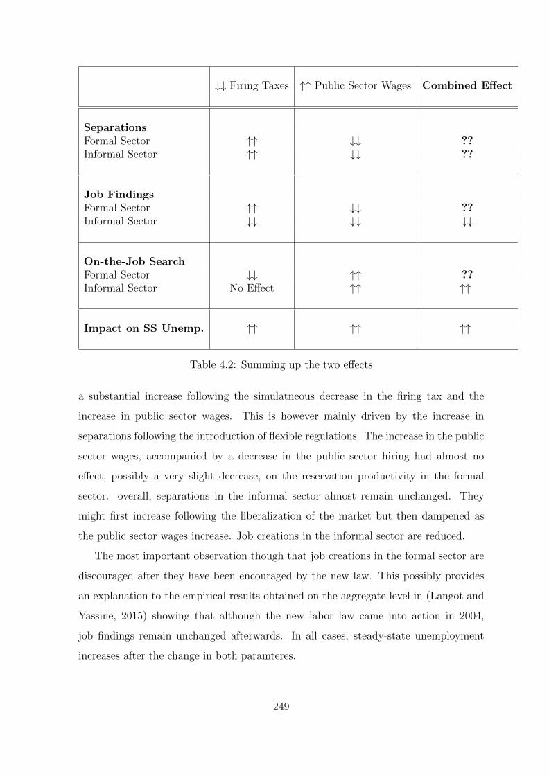
↓↓ Firing Taxes ↑↑ Public Sector Wages Combined Effect

SeparationsFormal Sector ↑↑ ↓↓ ??Informal Sector ↑↑ ↓↓ ??

Job FindingsFormal Sector ↑↑ ↓↓ ??Informal Sector ↓↓ ↓↓ ↓↓

On-the-Job SearchFormal Sector ↓↓ ↑↑ ??Informal Sector No Effect ↑↑ ↑↑

Impact on SS Unemp. ↑↑ ↑↑ ↑↑

Table 4.2: Summing up the two effects

a substantial increase following the simulatneous decrease in the firing tax and the

increase in public sector wages. This is however mainly driven by the increase in

separations following the introduction of flexible regulations. The increase in the public

sector wages, accompanied by a decrease in the public sector hiring had almost no

effect, possibly a very slight decrease, on the reservation productivity in the formal

sector. overall, separations in the informal sector almost remain unchanged. They

might first increase following the liberalization of the market but then dampened as

the public sector wages increase. Job creations in the informal sector are reduced.

The most important observation though that job creations in the formal sector are

discouraged after they have been encouraged by the new law. This possibly provides

an explanation to the empirical results obtained on the aggregate level in (Langot and

Yassine, 2015) showing that although the new labor law came into action in 2004,

job findings remain unchanged afterwards. In all cases, steady-state unemployment

increases after the change in both paramteres.

249

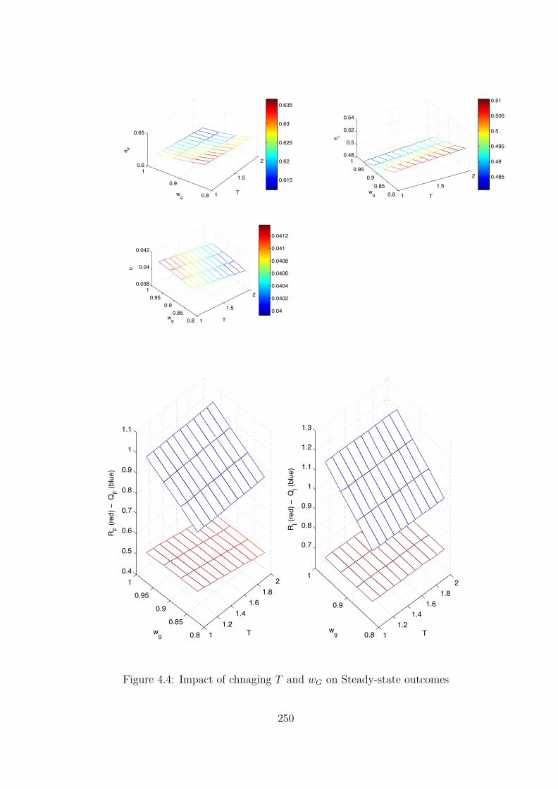
1

1.5

2

0.8

0.9

10.6

0.65

Twg

θ F

1

1.5

2

0.80.85

0.90.95

10.48

0.5

0.52

0.54

Twg

θ I

1

1.5

2

0.80.85

0.90.95

10.038

0.04

0.042

Twg

u

0.04

0.0402

0.0404

0.0406

0.0408

0.041

0.0412

0.615

0.62

0.625

0.63

0.635

0.485

0.49

0.495

0.5

0.505

0.51

11.2

1.41.6

1.82

0.8

0.85

0.9

0.95

10.4

0.5

0.6

0.7

0.8

0.9

1

1.1

Twg

RF (r

ed) −

QF (b

lue)

11.2

1.41.6

1.82

0.8

0.9

1

0.7

0.8

0.9

1

1.1

1.2

1.3

Twg

RI (r

ed) −

QI (b

lue)

Figure 4.4: Impact of chnaging T and wG on Steady-state outcomes

250

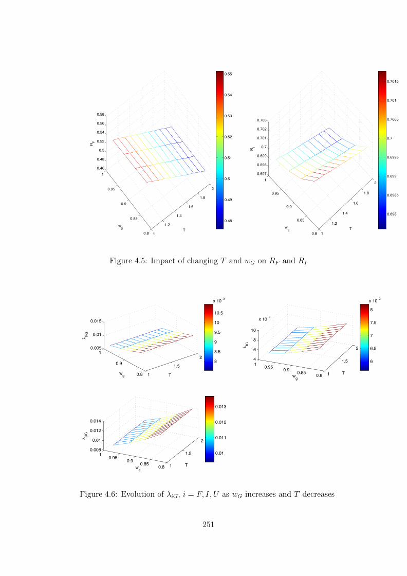
1

1.2

1.4

1.6

1.8

2

0.8

0.85

0.9

0.95

10.46

0.48

0.5

0.52

0.54

0.56

0.58

Twg

R F

1

1.2

1.4

1.6

1.8

2

0.8

0.85

0.9

0.95

10.697

0.698

0.699

0.7

0.701

0.702

0.703

Twg

R I

0.698

0.6985

0.699

0.6995

0.7

0.7005

0.701

0.7015

0.48

0.49

0.5

0.51

0.52

0.53

0.54

0.55

Figure 4.5: Impact of changing T and wG on RF and RI

1

1.5

2

0.8

0.9

10.005

0.01

0.015

Twg

λ FG

1

1.5

2

0.80.850.90.9514

6

8

10

x 10−3

Twg

λ IG

1

1.5

2

0.80.850.90.9510.008

0.01

0.012

0.014

Twg

λ UG

6

6.5

7

7.5

8

x 10−3

8

8.5

9

9.5

10

10.5

x 10−3

0.01

0.011

0.012

0.013

Figure 4.6: Evolution of λiG, i = F, I, U as wG increases and T decreases

251

4.5 Empirical Evidence from ELMPS 2012

In this section, we use the Egypt Labor Market Panel Survey, fielded in 2012 to

extract, as has been done in chapter 1, a longitudinal retrospective panel for the period

1998-2011. This allows us to construct time series for the job findings and separations

before and after the reform. The data also allows us to categorize employed workers

by sector of employment namely, public, formal and informal wage work. It has been

shown in chapters 2 and 3 that the retrospective panel extracted from the ELMPS

2012 suffer from a recall and design bias. Moreover, chapters 2 and 5 shows that the

characteristics of the sample are not kept random as we go back in time. Following

the correction methodology based on matching population moments and creating dif-

ferentiated weights, we are able to reconstruct corrected flows between the employment

sectors as well as unemployment5

Given these flows, we use the econometric methodology adopted in chapter 3 to

purge the time series of each type of transition, namely separations form formal and

informal sectors, job findings to the formal and informal sectors as well as transitions

from formal and informal sectors to the public sector, from the the macroeconomic

trend. The reform is then detected as a structural break in the series allowing us to

construct the counterfactual time series if the reform has not been implemented in

2004. To be able to estimate the impact of the reform on each type of flow, we model

the first approximation of the labor market flows as follows:

xt − x?t = α(yt − y?t ) + β + εt for x = sF , sI , fF , fI , λFG, λIG (4.42)

For i = F, I, si and fi are respectively the observed job finding and job separation

rates. λiG is the transition rate from a job in sector i to a job in the public sector. x?t

represents the natural rate of the labor market flows (whether job finding, separation

or transitions towards the public sector). yt is the log of the observed output and y?t

is the log of the potential output. The left-hand side term represents the flow gap,

5See chapters 1 and 2 for the raw labor market flows obtained form the ELMPS12 dataset. Theregressions in this section use the corrected flows.

252

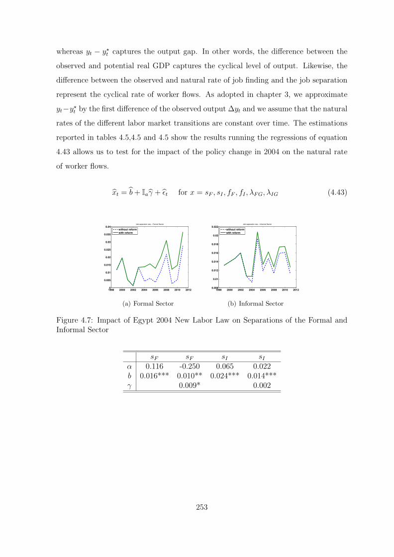
whereas yt − y?t captures the output gap. In other words, the difference between the

observed and potential real GDP captures the cyclical level of output. Likewise, the

difference between the observed and natural rate of job finding and the job separation

represent the cyclical rate of worker flows. As adopted in chapter 3, we approximate

yt−y?t by the first difference of the observed output ∆yt and we assume that the natural

rates of the different labor market transitions are constant over time. The estimations

reported in tables 4.5,4.5 and 4.5 show the results running the regressions of equation

4.43 allows us to test for the impact of the policy change in 2004 on the natural rate

of worker flows.

xt = b+ Iaγ + εt for x = sF , sI , fF , fI , λFG, λIG (4.43)

1998 2000 2002 2004 2006 2008 2010 20120

0.005

0.01

0.015

0.02

0.025

0.03

0.035

0.04

Job separation rate − Formal Sector

without reform

with reform

(a) Formal Sector

1998 2000 2002 2004 2006 2008 2010 20120.008

0.01

0.012

0.014

0.016

0.018

0.02

0.022

Job separation rate − Informal Sector

without reform

with reform

(b) Informal Sector

Figure 4.7: Impact of Egypt 2004 New Labor Law on Separations of the Formal andInformal Sector

sF sF sI sIα 0.116 -0.250 0.065 0.022b 0.016*** 0.010** 0.024*** 0.014***γ 0.009* 0.002

253

1998 2000 2002 2004 2006 2008 2010 20120

0.02

0.04

0.06

0.08

0.1

0.12

Job finding rate − Formal Sector

without reform

with reform

(a) Formal Sector

1998 2000 2002 2004 2006 2008 2010 20120.06

0.07

0.08

0.09

0.1

0.11

0.12

0.13

0.14

0.15

0.16

Job finding rate − Informal Sector

without reform

with reform

(b) Informal Sector

Figure 4.8: Impact of Egypt 2004 New Labor Law on Job Findings of the Formal andInformal Sector

fF fF fI fIα 0.628 0.307 -0.363 0.143b 0.044*** 0.052*** 0.010*** 0.010***γ -0.011 -0.000174

1998 2000 2002 2004 2006 2008 2010 20120.002

0.004

0.006

0.008

0.01

0.012

0.014

0.016

0.018

On−the−Job Search − Formal to Public

without reform

with reform

(a) Formal to Public

1998 2000 2002 2004 2006 2008 2010 20120.006

0.007

0.008

0.009

0.01

0.011

0.012

0.013

0.014

On−the−Job Search − Informal to Public

without reform

with reform

(b) Informal to Public

Figure 4.9: Impact of Egypt 2004 New Labor Law on the On-the-Job Search towardsthe Public Sector

λFG λFG λIG λIGα -0.064 -0.082 -0.025 -0.041b 0.010*** 0.011*** 0.009*** 0.009***γ -0.002 0.001

The results of these regressions using the ELMPS 2012 show that only the sepa-

rations in the formal sector increased significantly after the reform. The impact on

all other flows was insignificant. This however maybe due to the fact that we’re over

exploiting the data by detailing the transitions between the different employment sec-

tors, given the structure of the data set and the samples’ sizes discussed in chapter 1.

254

What is interesting however is that the direction of change in the natural rates of these

flows is coherent with the theoretical model presented in the previous section. Separa-

tions in both sectors increased showing that the effect of the reduced firing taxes has

dominated in that case. Findings in both sectors retreated slightly. For the informal

sector, this is due to both the decrease in the firing taxes as well as the increase in the

public sector wages. For the formal sector, it shows that the job creations were still

taxed by the increase in the public sector wages even though the hiring has declined.

Workers considering on-the-job search are now more than before. Interestingly how-

ever, this was not followed by more people really moving to the public sector. On the

contrary, actual transitions occurring to the public sector from the formal sector de-

creased. This comes however from the two contradicting forces acting in two different

directions; where decreasing firing taxes discouraged transitions to the public sector

while increasing public sector wages encouraged them. Since the firing taxes do not

have any effect on the on-the-job search towards the public sector in the informal jobs,

these increased following the rise in the public sector wages.

4.6 Conclusion

According to Assaad (2014), the dualism and segmented nature of MENA labor

markets plays an important role in their lack of dynamism. High levels of public sector

employment were used as part of the authoritarian bargain, where public employment

was exchanged for political acquiescence under authoritarian regimes. Labor was there-

fore allocated in line with political goals, which undermined the primary function of

labor markets, which is to distribute human capital to its most productive uses. With

an aim to portray the nature of labor markets in developing countries, we extend in

this paper a Mortensen-Pissarides model to add to the conventional private formal sec-

tor, public and informal wage employment sectors. The public sector is added as an

exogenous player where wage and employment policies are decided exogenously. How-

ever these policies are constrained by the government’s budget. The model shows the

different interactions between the sectors, and particularly endogenizes job creations,

job destructions as well as on-the job search towards the public sector, in both the

255

formal and the informal sector.

One example of a reform attempting but struggling to encourage dynamism in

MENA labor markets is observed in the case of Egypt. In Egypt, a new labor law

(Law 12 of 2003) was enacted with the goal of increasing the dynamism of the private

sector by making hiring and firing workers easier. Langot and Yassine (2015) (chapter

3) show using empirical evidence, that following the reform, modelled as a decrease in

the firing taxes imposed on employers, only separations increased significantly while

job findings hardly change. Trying to explain this partial failure of the reform, in

Langot and Yassine (2015) (chapter 3), we tried to adapt the Mortensen-Pissarides

model by adding corruption set up costs to explain such an empirical paradox. Yet,

another possible explanation might lie in the nature of the labor market of a developing

country such as Egypt, due to the existence of informal sectors and a sizeable public

employer. In the absence of a clear understanding of the inside story of the inter-

sectoral transitions, such policy reforms are unlikely to be effective and are unlikely to

achieve their objectives.

Using our model and numerical analysis, we show that the reduction in the firing

taxes increase job separations in both sectors formal and informal sectors. The reform

also discourages on-the-job search towards the public sector. Following the conven-

tional Mortensen-Pissarides mode, it is shown that job creations in the formal sector

is increased after a decrease in the firing taxes while job findings in the informal sector

is dampened. This is consistent with the fact that such reform aim at scaling down

the difference between formal and informal sectors by shifting employment towards the

formal sector by liberalizing it. An increase in formal job creations accompanied by a

decrease in informal job creations would result in ambiguous impact on the aggregate

job creations depending on the magnitude of each variation.

The new Labor law introduced in 2004 has however been accompanied simultane-

ously by a trending increase in the real wages of public sector workers, as proposed by

Said (2015). However, due to fiscal realities, this has been acompanied by less hiring

in the public sector. Both qualitative numerical analysis of the model and empirical

evidence from the data show that both formal and informal workers are encouraged

to search more on-the-job in the public sector. Moreover, simulating these variations,

256

the model reveals that the increase in public sector wages tends to nullify the positive

effect on the private formal sector’s job creation, it even reduces it. The increase in

public sector wages in this case acts as an extra taxation to the job creations in the

formal and informal sector. The net effect of observed after the 2004 Egypt labor law

is therefore an increase in the unemployment rates since job separations in all cases are

enhanced, but job creations remain unchanged or even dampened. This explains the

empirical paradox of the Egyptian case discussed in (Langot and Yassine, 2015), show-

ing that following the liberalization of the labor market, only job separations increase

and job findings remain unchanged. From a political evaluation point of view, the 2004

reform achieves its mission in liberalizing the market by favoring the formal sector to

the informal sector, boosting both its job creations and separations. These positive

effects, and particularly the increase in job creations, have been dampened and even

nullified by raising the levels of public sector wages at the same time. It becomes more

attractive to search for jobs in the public sector which becomes more remunerating.

Extensions: As has been explained in the paper, the model does not limit to

explaining the impact of firing taxes T and public sector wages wG. The aim is to

take this work further by testing for the impact of changes in other policy parameters

on the labor market equilibrium and generalizing the study to other developing labor

markets. Hiring subsidies, paryoll taxes and productivity shocks surely play important

roles in determining the different labor market outcomes. Another process that has been

neglected in this model and is worth exploring in a future research agenda is the jobs

formalization. Adding transitions from the informal to the formal sector to the model

might be interesting in terms of how the structure and segmentation of these labor

markets can get affected by the different policy parameters. For instance, liberalizing

the labor market not only that it favors creations from unemployment to the formal

sector but it surely favors transitions from informal jobs to formal ones. Endogenizing

productivities and when would jobs be formal or informal is also an interesting question

that can be used to extend the model.

257

References

Albrecht, J., L. Navarro, and S. Vroman (2009): “The Effects of Labour Market

Policies in an Economy with an Informal Sector*,” The Economic Journal, 119(539),

1105–1129.

Assaad, R. (2014): “Making sense of Arab labor markets: the enduring legacy of

dualism,” IZA Journal of Labor & Development, 3(1), 1–25.

Bosch, M., and J. Esteban-Pretel (2012): “Job creation and job destruction in

the presence of informal markets,” Journal of Development Economics, 98(2), 270–

286.

Bradley, J., F. Postel-Vinay, and H. Turon (2013): “Public sector wage policy

and labor market equilibrium: a structural model,” Unpublished manuscript, 2, 14.

Burdett, K. (2012): “Towards a theory of the labor market with a public sector,”

Labour Economics, 19(1), 68–75.

Charlot, O., F. Malherbet, and C. Terra (2015): “Informality in develop-

ing economies: Regulation and fiscal policies,” Journal of Economic Dynamics and

Control, 51, 1–27.

Charlot, O., F. Malherbet, and M. Ulus (2013): “Efficiency in a search and

matching economy with a competitive informal sector,” Economics Letters, 118(1),

192–194.

(2014): “Unemployment compensation and the allocation of labor in develop-

ing countries,” Journal of Public Economic Theory.

258

Diamond, P. A. (1981): “Mobility costs, frictional unemployment, and efficiency,”

The Journal of Political Economy, pp. 798–812.

(1982): “Wage determination and efficiency in search equilibrium,”The Review

of Economic Studies, 49(2), 217–227.

Langot, F., and C. Yassine (2015): “Reforming employment protection in Egypt:

An evaluation based on transition models with measurement errors,” Discussion pa-

per, Economic Research Forum, Cairo.

Meghir, C., R. Narita, and J.-M. Robin (2012): “Wages and informality in

developing countries,” Discussion paper, National Bureau of Economic Research.

Mortensen, D. T. (1978): “Specific capital and labor turnover,” The Bell Journal of

Economics, pp. 572–586.

(1982): “The matching process as a noncooperative bargaining game,” in The

economics of information and uncertainty, pp. 233–258. University of Chicago Press.

Mortensen, D. T., and C. A. Pissarides (1994): “Job creation and job destruction

in the theory of unemployment,” The review of economic studies, 61(3), 397–415.

(2001): “Taxes, subsidies and equilibrium labour market outcomes,” Discus-

sion paper, CEPR.

Petrongolo, B., and C. A. Pissarides (2001): “Looking into the black box: A

survey of the matching function,” Journal of Economic literature, pp. 390–431.

Pissarides, C., R. Layard, and M. Hellwig (1986): “Unemployment and vacan-

cies in Britain,” Economic policy, pp. 500–559.

Pissarides, C. A. (1990): Equilibrium unemployment theory. MIT press.

Said, M. (2015): “JWages and inequality in the Egyptian labor market in an era of

financial crisis and revolution,” Discussion paper, Economic Research Forum, Cairo.

Yassine, C. (2014): “Job Accession, Separation and Mobility in the Egyptian Labor

Market over the Past Decade,” Discussion paper, Economic Research Forum, Cairo.

259

4.A Deriving the Market’s Surplus

Formal Sector

The initial surplus in the formal sector is defined as S0F = J0

F − VF − pF (C −H) +

W 0F (1) − U , while the continuing job surplus is SF (x) = maxJNSF (x) + pFT − VF +

WNSF (x)− U, JSF (x) + pFT − VF +W S

F (x)− U.

At the time of hiring, when the idiosyncratic component is at its highest value x = 1

, the initial match surplus in the formal sector is therefore :

(r + δ + λF )S0F (1) = pF + τ + λF

∫ 1

RF

SF (z)dFF (z)− (r + δ)(U + VF )

− (r + δ + λF )pF (C −H)− λFpFT (4.44)

For a continuing match, and in case on-the-job search takes place i.e. if x ≤ QF ,

the surplus of the job, SSF (x) solves the following equation:

(r + δ + λF + λFG)SSF (x) = pFx+ τ + λF

∫ 1

RF

SF (z)dFF (z) + (r + δ + λFG)pFT

− (r + δ)(VF + U) + λFG(WG − U) (4.45)

If x > QF , the workers do not search on-th-job for better options in the public sector.

The only outside option in this case is the destruction of the job and the worker

becoming unemployed. The surplus, SNSF (x), in this case solves the following equation:

(r + δ + λF )SNSF (x) = pFx+ τ + λF

∫ 1

RF

SF (z)dFF (z)− (r + δ)(VF − pFT + U)

Since the separation rule has to maximize the total wealth in a bilateral agreement,

we know that J(RF ) + W (RF ) = VF − pFT + U , where j = S,NS. It follows that

SjF (RF ) = 0. This allows us to derive SSF (x) as

SSF (x) =pF (x−RF )

r + δ + λF + λFG(4.46)

260

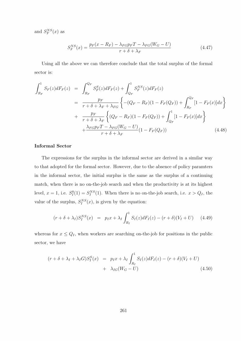
and SNSF (x) as

SNSF (x) =pF (x−RF )− λFGpFT − λFG(WG − U)

r + δ + λF(4.47)

Using all the above we can therefore conclude that the total surplus of the formal

sector is:

∫ 1

RF

SF (z)dFF (z) =

∫ QF

RF

SSF (z)dFF (z) +

∫ 1

QF

SNSF (z)dFF (z)

=pF

r + δ + λF + λFG

−(QF −RF )(1− FF (QF )) +

∫ QF

RF

[1− FF (x)]dx

+

pFr + δ + λF

(QF −RF )(1− FF (QF )) +

∫ 1

QF

[1− FF (x)]dx

+λFGpFT − λFG(WG − U)

r + δ + λF(1− FF (QF )) (4.48)

Informal Sector

The expressions for the surplus in the informal sector are derived in a similar way

to that adopted for the formal sector. However, due to the absence of policy paramters

in the informal sector, the initial surplus is the same as the surplus of a continuing

match, when there is no on-the-job search and when the productivity is at its highest

level, x = 1, i.e. S0I (1) = SNSI (1). When there is no on-the-job search, i.e. x > QI , the

value of the surplus, SNSI (x), is given by the equation:

(r + δ + λI)SNSI (x) = pIx+ λI

∫ 1

RI

SI(z)dFI(z)− (r + δ)(VI + U) (4.49)

whereas for x ≤ QI , when workers are searching on-the-job for positions in the public

sector, we have

(r + δ + λI + λIG)SSI (x) = pIx+ λI

∫ 1

RI

SI(z)dFI(z)− (r + δ)(VI + U)

+ λIG(WG − U) (4.50)

261

Since SSI (RI) = 0, subtracting SSI (RI) from SSI (x) allows us to obtain:

SSI (x) =pI(x−RI)

r + δ + λI + λIG(4.51)

and subtracting SSI (RI) from SNSI (x) gives:

SNSI (x) =pI(x−RI)− λIG(WG − U)

r + δ + λI(4.52)

Using all the above we can therefore conclude that the total surplus in the informal

sector is derived as follows:

∫ 1

RI

SI(z)dFI(z) =

∫ QI

RI

SSI (z)dFI(z) +

∫ 1

QI

SNSI (z)dFI(z)

=pI

r + δ + λI + λIG

−(QI −RI)(1− FI(QI)) +

∫ QI

RI

[1− FI(x)]dx

+

pIr + δ + λI

(QI −RI)(1− FI(QI)) +

∫ 1

QI

[1− FI(x)]dx

+λIG(1− FI(Q1))

r + δ + λI(WG − U) (4.53)

262

Part III

Quality of Jobs and Labor Market

Search Frictions

263

Chapter 5

Constructing Labor Market

Transitions Weights in

Retrospective Data: An

Application to Egypt and Jordan 1

5.1 Introduction

As has been well established in the previous chapters, researchers, demographers

and policy makers in the MENA region became increasingly interested in understanding

employment histories or the worker’s life course after schooling, with a focus on events,

their sequence, ordering and transitions that people make from one labor market state

to another. The Arab Spring countries, in particular, are currently continously debating

on how to respond to the economic crises and also on how to provide more equitable

opportunities through their labor markets. Consequently, policy-relevant research on

labor market dynamics becomes particularly valuable.

Given that there are no official statistics on labor market dynamics in the MENA

1Acknowledgements are due to Francois Langot and David Margolis for all the discussions, helpand guide provided through out the different phases of this paper. I would like to thank AntoineTerracol and Govert Bijwarrd for their generosity to share their STATA do files on duration models.Insan Tunali, Ragui Assaad, Jackline Wahba and Aysit Tansel provided very useful comments. Igratefully acknowledge financial support from the Economic Research Forum, grant ERF2014-050 forthe paper, as part of the project “Labor Market Dynamics in the Middle East and North Africa”.

264

region, as has been explained in parts I and II of this thesis, very little research has

so far been done on the issue in the region. It has also been shown that in order to

assess labor market dynamics in the two countries in question (Egypt and Jordan),

detailed annual panel data on labor market statuses is required. The only possible

way to obtain such panel data is to extract longitudinal retrospective panel datasets

from the Egypt Labor Market Panel Survey fielded in 2006 and 2012 (ELMPS 2006

and 2012), and the Jordan Labor Market Panel Survey fielded in 2010 (JLMPS 2010).

Yassine (2015) and Assaad, Krafft, and Yassine (2015) (part I in this thesis) explain

that these datasets provide detailed labor market histories for those who ever worked

as well as current employment/non-employment information for all interviewed indi-

viduals. This consequently allows the creation of retrospective longitudinal panels of

the individuals’ labor market states on an annual or semi-annual basis, going back in

time from the year of the survey for each country. These retrospective panels suffer

however from measurement errors. According to Langot and Yassine (2015) (chapter

3) and Assaad, Krafft, and Yassine (2015) (chapter 2), the retrospective information

obtained from these surveys suffer from what is referred to as recall and design bias.

Recall bias is defined as respondents mis-reporting their retrospective trajectory be-

cause they tend to forget some events or spells, especially the short ones. The design

bias arises from the fact that different types of questions are being asked for current

versus recall/retrospective statuses. There is therefore a question of salience/cognitive

recognition by the respondents where by asking the questions differently, respondents,

or even sometimes the enumerators, can interpret them differently. Yassine (2015)

(chapter 1) and Assaad, Krafft, and Yassine (2015) (chapter 2) show for instance that

due to the design of the questionnaires of the ELMPS and the JLMPS, statuses in the

retrospective sections are sometimes being interpreted more of job statuses rather than

labor market states. Langot and Yassine (2015) proposes a methodology to correct for

this bias producing corrected aggregate transition rates obtained from the retrospec-

tive data. This methodology assumes that the contemporaneous (panel data) aggregate

transition rates, obtained from the ELMPS 1998, 2006 and 2012, are the correct ones 2.

2See Assaad, Krafft, and Yassine (2015) (chapter 2) and Langot and Yassine (2015) (chapter 3)for more details.

265

The latter approach therefore limits to analyzing the macro aggregate indicators (time

series) of the labor market transitions. Exploiting the micro-level individual informa-

tion available on the workers’ and jobs’ characteristics underlying these transitions is

however very important, especially if available in the data. Characterizing movements

within the labor market, for instance, can help policy makers design various effective

policies to address unemployment, informality or non-participation and reduce their

adverse consequences. Tansel and Ozdemir (2015) provided an analysis of labor mar-

ket dynamics in Egypt with an emphasis on formal/informal labor market states using

contemporaneous panel data for the period 2006-2012, showing that increasing educa-

tion levels can play an important role in reducing transitions into informal states of

labor market. Their paper however studies labor market transitions over a period of

six years. A lot of incidents and transitions can occur in between and these transitions

need to be assessed on at least an annual basis.

This paper therefore builds on the methodology proposed by Langot and Yassine

(2015) (chapter 3) and extends it to correct the data on the individual transaction

level (i.e. micro level). The model proposed in this paper creates user-friendly weights

that can be readily used by researchers relying on the ELMPS and JLMPS retrospective

panels. The recall and design bias in the data cannot be ignored. As has been clarified in

Bound, Brown, and Mathiowetz (2001), errors (even if random) in categorical or binary

variables (which is the case of labor market transitions) are problematic. Whether

the mis-measured variable is the dependant or independent variable, the regression

estimates would be biased downwards (attenuated). In Assaad, Krafft, and Yassine

(2015) (chapter 2), it was also shown that these errors are systematic i.e. related

to covariates. Such relationships will bias any attempts to examine the relationship

between covariates and mis-measured outcomes. Consequently, one can not ignore

such measurement errors and the results of the applications shown at the end of this

paper support this argument. Moreover, given the nature and the sample sizes of

the datasets used, it’s not possible to structurally estimate the bias, simultaneously

with the estimation of any other model. First, the JLMPS is the first wave of the

survey in Jordan. The retrospective responses can therefore not be overlapped with

contemporaneous responses from another wave to identify whether an individual is mis-

266

reporting a labor market state in the past. Even when other waves are available as in the

case of Egypt, the number of individuals who were interviewed in both surveys and can

therefore be identified for mis-reporting, provides small sized samples when classified

by the type of transitions (see Appendix 1.B in Chapter 1). These are even the sizes of

the samples before categorizing them by observable characteristics, which means that

estimations in that case would be based in some cases on only one observation, if not

sometimes none.

The technique suggested by this paper shows that it is sufficient to have popu-

lation, stocks and transitions, moments to correct over- or under-reporting biases in

retrospective data. The true unbiased moments can be obtained from auxiliary infor-

mation such as contemporaneous information from other waves of the same survey, or

even external data sources, so long comparability between the varaibles’ definitions is

verified. Once the moments are matched on the aggregate level, a measurement error

for each type of transition at a point in time t is estimated. This measurement error is

then distributed among the sample’s individual observations/transactions in the form

of micro-data weights, such as observations that are being under-reported take higher

weights and those over-reported take lower weights. The paper proposes two types of

weights: (1)naive proportional weights and (2)differentiated predicted weights. Naive

proportional weights offer the advantage of being simple to calculate and handy. How-

ever, Assaad, Krafft, and Yassine (2015) show that not only retrospective data will

under-report past unemployment but also distort its characteristics. The retrospective

panels are therefore not random. In an attempt, to re-obtain random samples within

these panels, the differentiated predicted weights are constructed. Following an accu-

rate random sample (which in our case is the most recent year of the retrospective

panels), one can estimate the probability for an individual to make a specific type of

labor market transition as a function of observable characteristics. If the individual is

more probable to transit, then he is more probable to mis-report. Distributing the mea-

surement error among the sample’s observations according to these probabilities, via

differentiated weights, allows to redress the retrospective panels into random samples

readily used for micro-data analysis of labor market dynamics. Both transaction-level

weights i.e. for each transition at a certain point in time, as well as panel weights i.e.

267

for an entire spell are built. In order to highlight the importance of these weights, the

last section of this paper offers an application using these weights. The determinants

of labor market transitions are analyzed via a multinomial regression analysis with

and without the weights. The impact of these weights on the regressions estimations

and coefficients is therefore examined and shown significant among the different labor

market transitions, particularly separations.

The application demonstrated in this paper using the recall weights allows to esti-

mate the markov transition probabilities for labor market states over time as function

of observable characteristics. On the one hand such analysis allows to point out the

chances of transitioning between and within employment and non-employment states.

On the other hand, the obtained estimations are suggestive of the roles of state depen-

dence in these labor market transitions. The markov transition probabilities are mainly

estimated between the three labor market states, namely employment, unemployment

and inactivity, over time as function of observable worker’s, firm’s characteristics as

well as macroeconomic indicators such as labor market tightness. The paper also

provides desaggregated labor market transitions, when possible, namely public wage

work, private formal wage work, private informal wage work, self-employment and non-

employment. Although it was not possible, given the samples’ sizes and the nature of

transitions, to construct the recall weights for female workers, transition probabilities

using a gender-specific multinomial logit specification were predicted. The tansition

matrices are conditioned on different individual characteristics like gender, age, region

of residence...etc and firm/job characteristics such as the size of the firm, the sector of

employment..etc.

The rest of the paper is structured as follows. The next section describes the data

treatment and the creation of transitions and panel weights. Section 3 surveys corrected

and uncorrected descriptive statistics, as well as a counting analysis of the transition

matrices. Section 4 provides an application showing results from multinomial logit

regression models. Section 5 concludes.

268

5.2 Creating Weights

5.2.1 Data and Sampling

Data from Egypt and Jordan are used. The three rounds of the Egypt Labor Mar-

ket Panel Survey (ELMPS), fielded in 1998, 2006 and 2012 and the first round of the

Jordan Labor Market Panel Survey (JLMPS) fielded in 2010 are exploited. The two

surveys are nationally representative including both detailed current employment and

nonemployment information as well as labor market histories that allow for an assess-

ment of employment and nonemployment transitions and spells’ durations. The surveys

elicit information on detailed individual characteristics as well as job (or firm) charac-

teristics. Following the methodology and assumptions adopted by (Yassine, 2015), a

retrospective longitudinal panel dataset is extracted for each country, going back ten

years from the year of the survey, i.e. 2001-2011 for Egypt, and 2000-2010 for Jordan

3.

The sample used in this paper includes male individuals between 15 and 49 years

of age. The sample includes those who ever worked, the young unexperienced new

labor market entrants and the individuals who are permanently out of the labor force.

Female workers in this context are being excluded since their behaviour of entry and

exit into/from the labor market is likely to be driven by personal motives such as

marriage and child birth. Theory and steady-state assumptions made in the recall

correction model can therefore be distorted and might not be fully applicable if female

workers are included in the analysis. Female individuals between 15 and 49 years of

age are also added to the analysis when non-corrected gender-specific regressions are

estimated.

3As the surveys are fielded at the begining of the survey year, the last year’s transitions arenot captured fully and are therefore ommitted from the observation period. For Jordan, the casewas exceptional, even though the survey was fielded from February to April 2014 i.e during the firstsemester of the year, whether 2009/2010 was included or not to the analysis, the same results areobtained. It has been therefore opted to keep 2009/2010 in the analysis for sample size reasons.

269

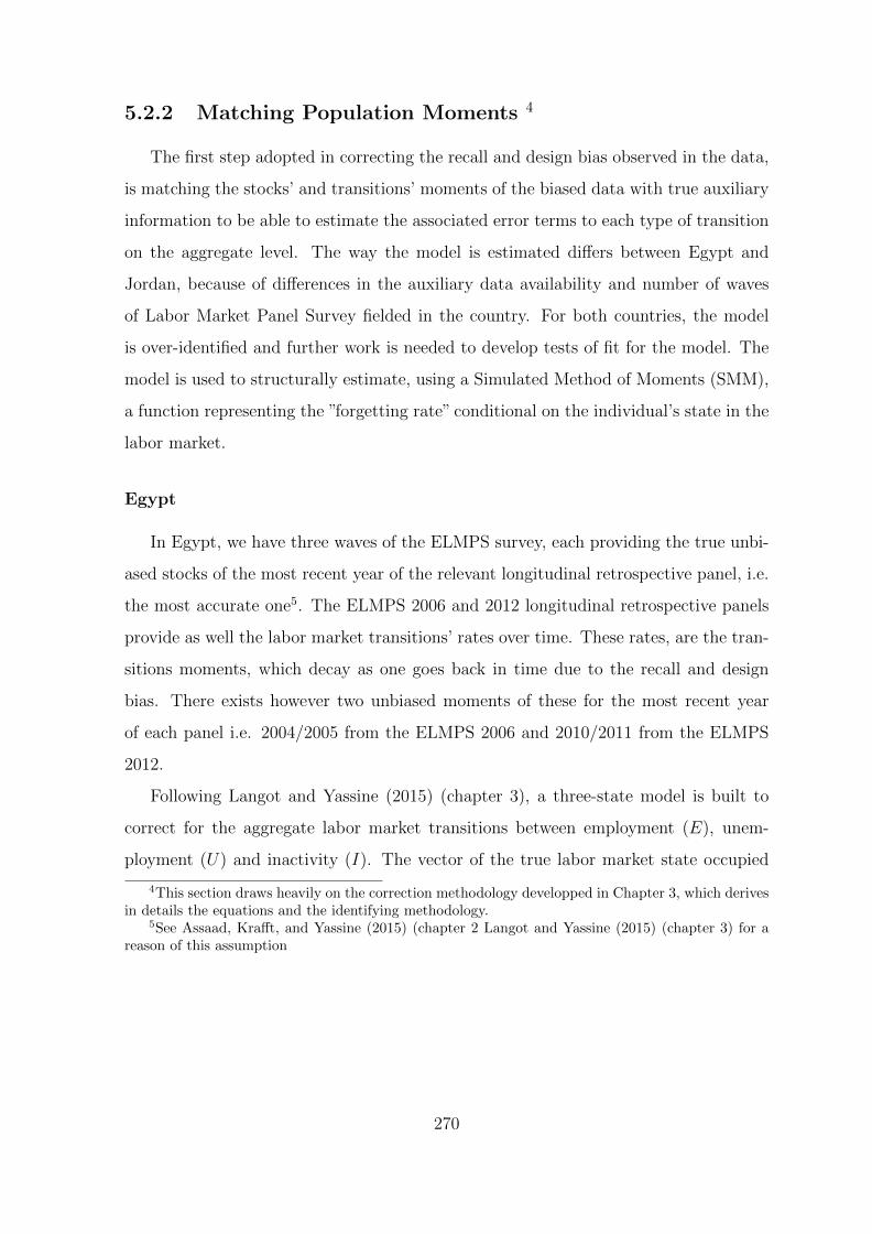
5.2.2 Matching Population Moments 4

The first step adopted in correcting the recall and design bias observed in the data,

is matching the stocks’ and transitions’ moments of the biased data with true auxiliary

information to be able to estimate the associated error terms to each type of transition

on the aggregate level. The way the model is estimated differs between Egypt and

Jordan, because of differences in the auxiliary data availability and number of waves

of Labor Market Panel Survey fielded in the country. For both countries, the model

is over-identified and further work is needed to develop tests of fit for the model. The

model is used to structurally estimate, using a Simulated Method of Moments (SMM),

a function representing the ”forgetting rate” conditional on the individual’s state in the

labor market.

Egypt

In Egypt, we have three waves of the ELMPS survey, each providing the true unbi-

ased stocks of the most recent year of the relevant longitudinal retrospective panel, i.e.

the most accurate one5. The ELMPS 2006 and 2012 longitudinal retrospective panels

provide as well the labor market transitions’ rates over time. These rates, are the tran-

sitions moments, which decay as one goes back in time due to the recall and design

bias. There exists however two unbiased moments of these for the most recent year

of each panel i.e. 2004/2005 from the ELMPS 2006 and 2010/2011 from the ELMPS

2012.

Following Langot and Yassine (2015) (chapter 3), a three-state model is built to

correct for the aggregate labor market transitions between employment (E), unem-

ployment (U) and inactivity (I). The vector of the true labor market state occupied

4This section draws heavily on the correction methodology developped in Chapter 3, which derivesin details the equations and the identifying methodology.

5See Assaad, Krafft, and Yassine (2015) (chapter 2 Langot and Yassine (2015) (chapter 3) for areason of this assumption

270

at year t is

Y (t) =

E(t)

U(t)

I(t)

(5.1)

where E(t), U(t) and I(t) represent the true proportion of employed, unemployed and

inactive individuals respectively in year t (i.e. the unbiased moments of the population

stocks). The vector

y(t) =

e(t)

u(t)

i(t)

(5.2)

denotes the observed empirical labor market state proportions at time t, with e(t), u(t)

and i(t) being the observed proportion of employed, unemployed and inactive in year

t. With λlk(t−1, t) being the transition rates from state l occupied in t−1 to the state

k occupied in t, the matrix

N(t− 1, t) =

λEE(t− 1, t) λEU(t− 1, t) λEI(t− 1, t)

λUE(t− 1, t) λUU(t− 1, t) λUI(t− 1, t)

λIE(t− 1, t) λIU(t− 1, t) λII(t− 1, t)

(5.3)

gives the observed transition probabilities between the year t− 1 and the year t. These

are obtained by aggregating the expanded number of individuals making the transition

lk from the year t− 1 to year t in the constructed retrospective panels and dividing by

the stock of l in the year t − 16. This resembles the methodology adopted by Shimer

(2012) to extract macro time-series of labor market flows from individual transaction-

level micro-data. There exists a restriction on these transition rates: the sum of the

elements of each column must be equal to one. Thus, we have:

λEI(t− 1, t) = 1− λEU(t− 1, t)− λEE(t− 1, t) (5.4)

6See chapter 1 for the way flows, such as job finding and separation rates, are being calculated

271

λUI(t− 1, t) = 1− λUE(t− 1, t)− λUU(t− 1, t) (5.5)

λIU(t− 1, t) = 1− λIE(t− 1, t)− λII(t− 1, t) (5.6)

This transition matrix in equation 5.3 leads to

y(t) = N ′(t− 1, t)y(t− 1) (5.7)

As previously mentioned, the observed transition probabilities are biased due to recall

or design issues. An error term ϕz(t − 1, t), for z = E,U, I, is therefore defined and

associated to the z-type agents. These error terms vary in time and increase as one

goes back in history, showing the loss of accuracy and memory as older events are

being reported. The true matrix of transition probabilities between years t − 1 and t

can therefore be written as follows;

Ω(t− 1, t) =

λEE − ϕE λEU + a1ϕE λEI + (1− a1)ϕE

λUE + b1ϕU λUU − ϕU λUI + (1− b1)ϕg

λIE + c1ϕI λIU + (1− c1)ϕI λII − ϕI

=

λEE − ϕE λEU + a1ϕE (1− λEE − λEU) + (1− a1)ϕE

λUE + b1ϕU λUU − ϕU (1− λUE − λUU) + (1− b1)ϕU

λIE + c1ϕI (1− λIE − λII) + (1− c1)ϕI λII − ϕI

(5.8)

The above correction therefore allows to obtain:

Y (t) = Ω′(t− 1, t)Y (t− 1) (5.9)

where Ω′(t− 1, t) is the transposed matrix of Ω(t− 1, t). A parametric functional form

is imposed on these error terms ϕz(t− 1, t) :

ϕz(t− 1, t) = νz(1− exp(−θz(T − t)))

272

implying ϕz(T − 1, T ) = 0 , i.e. assuming that the transition rates are correctly

estimated for the most recent year T of the survey (as per the descriptive statis-

tics shown in chapters 2 and 3). For the correction of the transition rates obtained

from the ELMPS 2012, this characteristic becomes very useful and allows one to

write Ω(T − 1, T ) = N(T − 1, T ) for a given extracted retrospective panel data set.

For the 2012 round, the assumption Ω(2010, 2011) = N(2010, 2011) is made and

Ω(2004, 2005) = N(2004, 2005) for the 2006 round. This reflects that the most re-

cent year of the retrospective panel extracted from a survey is the most accurate one.

Given this three-state setting, one is able to estimate the parameters

Θ3 = θE, θU , θI , νE, νU , νI , a1, b1, c1

where dim(Θ3) = 9, by solving the following system

g(xT ,Θ3) =

Y (2011)ELMPS12

Y (2005)ELMPS06

λEE(2004, 2005)|2006

λUU(2004, 2005)|2006

λII(2004, 2005)|2006

λEU(2004, 2005)|2006

λUE(2004, 2005)|2006

λIE(2004, 2005)|2006

−

Ω1(Θ3)

Ω2(Θ3)

Ω3(Θ3)

Ω4(Θ3)

Ω5(Θ3)

Ω6(Θ3)

Ω7(Θ3)

Ω8(Θ3)

= [ψT − ψ(Θ3)] (5.10)

273

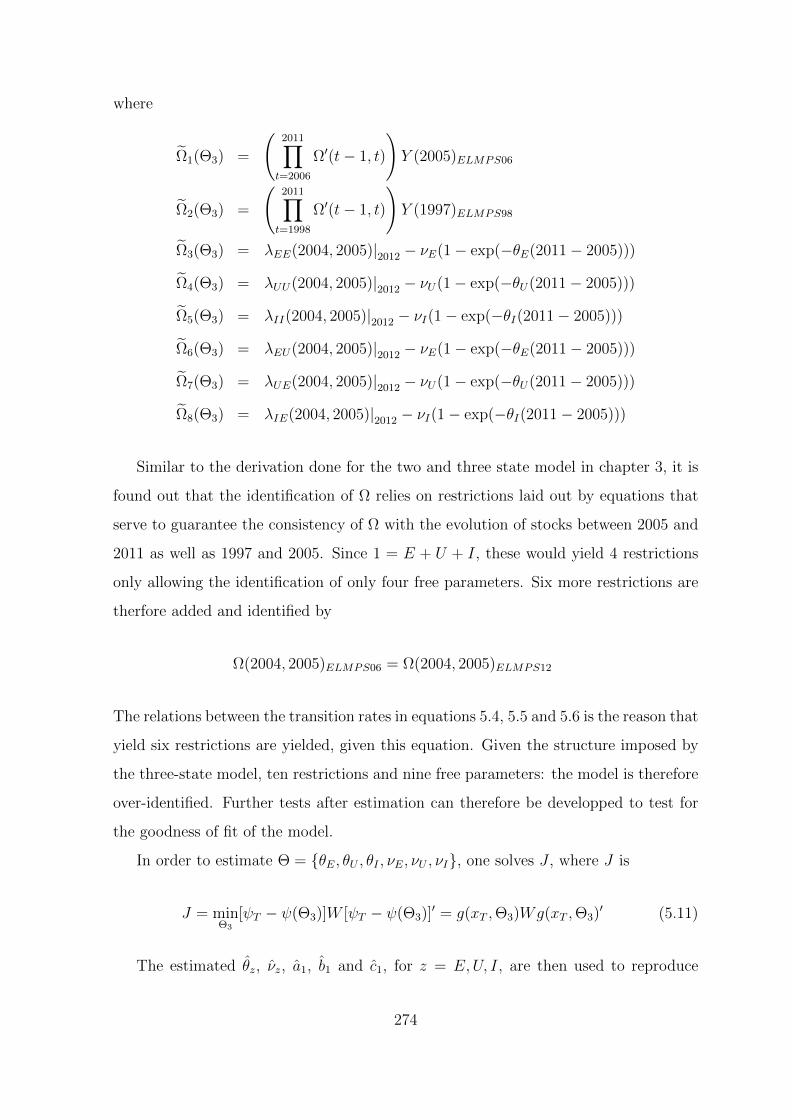
where

Ω1(Θ3) =

(2011∏t=2006

Ω′(t− 1, t)

)Y (2005)ELMPS06

Ω2(Θ3) =

(2011∏t=1998

Ω′(t− 1, t)

)Y (1997)ELMPS98

Ω3(Θ3) = λEE(2004, 2005)|2012 − νE(1− exp(−θE(2011− 2005)))

Ω4(Θ3) = λUU(2004, 2005)|2012 − νU(1− exp(−θU(2011− 2005)))

Ω5(Θ3) = λII(2004, 2005)|2012 − νI(1− exp(−θI(2011− 2005)))

Ω6(Θ3) = λEU(2004, 2005)|2012 − νE(1− exp(−θE(2011− 2005)))

Ω7(Θ3) = λUE(2004, 2005)|2012 − νU(1− exp(−θU(2011− 2005)))

Ω8(Θ3) = λIE(2004, 2005)|2012 − νI(1− exp(−θI(2011− 2005)))

Similar to the derivation done for the two and three state model in chapter 3, it is

found out that the identification of Ω relies on restrictions laid out by equations that

serve to guarantee the consistency of Ω with the evolution of stocks between 2005 and

2011 as well as 1997 and 2005. Since 1 = E + U + I, these would yield 4 restrictions

only allowing the identification of only four free parameters. Six more restrictions are

therfore added and identified by

Ω(2004, 2005)ELMPS06 = Ω(2004, 2005)ELMPS12

The relations between the transition rates in equations 5.4, 5.5 and 5.6 is the reason that

yield six restrictions are yielded, given this equation. Given the structure imposed by

the three-state model, ten restrictions and nine free parameters: the model is therefore

over-identified. Further tests after estimation can therefore be developped to test for

the goodness of fit of the model.

In order to estimate Θ = θE, θU , θI , νE, νU , νI, one solves J , where J is

J = minΘ3

[ψT − ψ(Θ3)]W [ψT − ψ(Θ3)]′ = g(xT ,Θ3)Wg(xT ,Θ3)′ (5.11)

The estimated θz, νz, a1, b1 and c1, for z = E,U, I, are then used to reproduce

274

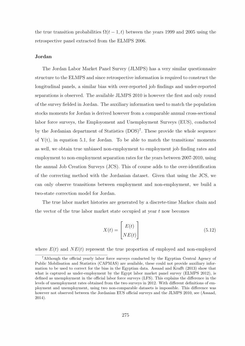
the true transition probabilities Ω(t− 1, t) between the years 1999 and 2005 using the

retrospective panel extracted from the ELMPS 2006.

Jordan

The Jordan Labor Market Panel Survey (JLMPS) has a very similar questionnaire

structure to the ELMPS and since retrospective information is required to construct the

longitudinal panels, a similar bias with over-reported job findings and under-reported

separations is observed. The available JLMPS 2010 is however the first and only round

of the survey fielded in Jordan. The auxiliary information used to match the population

stocks moments for Jordan is derived however from a comparable annual cross-sectional

labor force surveys, the Employoment and Unemployment Surveys (EUS), conducted

by the Jordanian department of Statistics (DOS)7. These provide the whole sequence

of Y(t), in equation 5.1, for Jordan. To be able to match the transitions’ moments

as well, we obtain true unbiased non-employment to employment job finding rates and

employment to non-employment separation rates for the years between 2007-2010, using

the annual Job Creation Surveys (JCS). This of course adds to the over-identification

of the correcting method with the Jordanian dataset. Given that using the JCS, we

can only observe transitions between employment and non-employment, we build a

two-state correction model for Jordan.

The true labor market histories are generated by a discrete-time Markov chain and

the vector of the true labor market state occupied at year t now becomes

X(t) =

E(t)

NE(t)

(5.12)

where E(t) and NE(t) represent the true proportion of employed and non-employed

7Although the official yearly labor force surveys conducted by the Egyptian Central Agency ofPublic Mobilisation and Statistics (CAPMAS) are available, these could not provide auxiliary infor-mation to be used to correct for the bias in the Egyptian data. Assaad and Krafft (2013) show thatwhat is captured as under-employment by the Egypt labor market panel survey (ELMPS 2012), isdefined as unemployment in the official labor force surveys (LFS). This explains the difference in thelevels of unemployment rates obtained from the two surveys in 2012. With different definitions of em-ployment and unemployment, using two non-comparable datasets is impossible. This difference washowever not observed between the Jordanian EUS official surveys and the JLMPS 2010, see (Assaad,2014).

275

respectively in the labor force in year t. These are therefore the unbiased true moments

of the population stocks obtained from the data. The vector

x(t) =

e(t)ne(t)

(5.13)

denotes the observed empirical labor market state proportions at time t, with e(t) and

ne(t) being the observed proportion of employed and unemployed in the labor force in

year t. These are the observed moments that decay, i.e. get biased due to the recall

and design measurement errors as one goes back in time from the year of the survey.

With λlk(t− 1, t) being the transition rates from state l occupied in t− 1 to the state

k occupied in t, the matrix

M(t− 1, t) =

λE−E(t− 1, t) λE−NE(t− 1, t)

λNE−E(t− 1, t) λNE−NE(t− 1, t)

8 (5.14)

gives the observed transition probabilities between the year t− 1 and the year t. These

are obtained by aggregating the expanded number of individuals making the transition

lk from the year t− 1 to year t in the constructed retrospective panels and dividing by

the stock of l in the year t− 1. There exists a restriction on these transition rates: the

sum of the elements of each column must be equal to one,

λE−NE(t− 1, t) = 1− λEE(t− 1, t) (5.15)

λNE−E(t− 1, t) = 1− λNE−NE(t− 1, t) (5.16)

The transition matrix in equation 5.14 leads to

x(t) = M ′(t− 1, t)x(t− 1) (5.17)

where M ′(t−1, t) is the transposed matrix of M(t−1, t). The observed transition prob-

abilities, as have been explained above, are biased due to recall and design measurement

errors. To be able to correct this bias, an error term ϕz(t− 1, t), for z = E,NE, is de-

fined and associated to the z-type agents. These error terms vary in time and increase

276

as one goes back in history, showing the loss of accuracy and memory as older events

are being reported, as observed in the descriptive statistics in the previous section.

The true matrix of transition probabilities between years t− 1 and t can therefore be

written as follows;

Π(t− 1, t) =

λE−E(t− 1, t)− ϕE(t− 1, t) λE−NE(t− 1, t) + ϕE(t− 1, t)

λNE−E(t− 1, t) + ϕNE(t− 1, t) λNE−NE(t− 1, t)− ϕNE(t− 1, t)

=

λE−E(t− 1, t)− ϕE(t− 1, t) 1− [λE−E(t− 1, t)− ϕE(t− 1, t)]

1− [λNE−NE(t− 1, t)− ϕNE(t− 1, t)] λNE−NE(t− 1, t)− ϕNE(t− 1, t)

(5.18)

By correcting the observed transition matrix M(t − 1, t), in equation 5.14 and

obtaining a true corrected one Π(t− 1, t), in equation 5.18, we obtain

X(t) = Π′(t− 1, t)X(t− 1) (5.19)

where Π′(t−1, t) is the transposed matrix of Π(t−1, t). For simplicity, the error terms

ϕz(t−1, t), for z = E,NE, are assumed to have the same functional form as in Egypt9

:

ϕz(t− 1, t) = νz(1− exp(−θz(T − t))) (5.20)

implying ϕz(T−1, T ) = 0. The worker flows are correctly estimated for the most recent

year T , we therefore assume that Π(T − 1, T ) = M(T − 1, T ) for a given retrospective

panel data set. The assumption Π(2009, 2010) = M(2009, 2010) is therefore made.

The parameters Θ = θE, θNE, νE, νNE are estimated given the above setting and

available data, using a Simulated Method of Moments (SMM). We solve the following

9Further work is needed to expand on the role of this parametric assumption and to check to whatextent this affects the results.

277

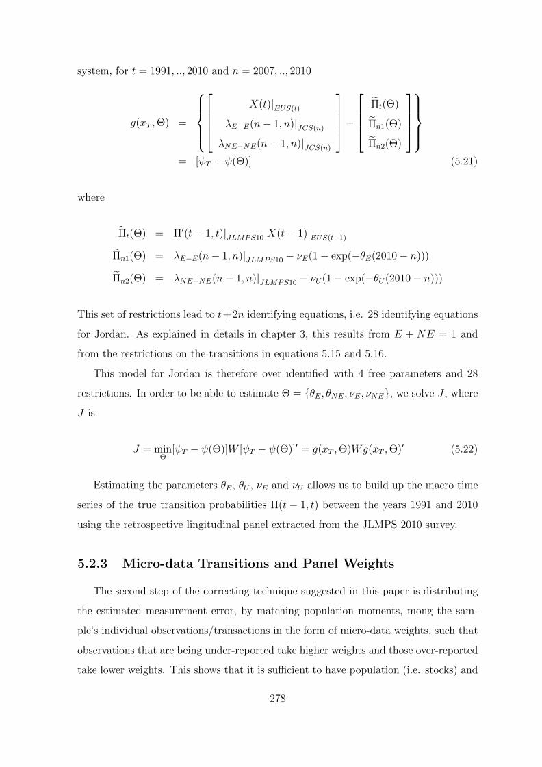
system, for t = 1991, .., 2010 and n = 2007, .., 2010

g(xT ,Θ) =

X(t)|EUS(t)

λE−E(n− 1, n)|JCS(n)

λNE−NE(n− 1, n)|JCS(n)

−

Πt(Θ)

Πn1(Θ)

Πn2(Θ)

= [ψT − ψ(Θ)] (5.21)

where

Πt(Θ) = Π′(t− 1, t)|JLMPS10 X(t− 1)|EUS(t−1)

Πn1(Θ) = λE−E(n− 1, n)|JLMPS10 − νE(1− exp(−θE(2010− n)))

Πn2(Θ) = λNE−NE(n− 1, n)|JLMPS10 − νU(1− exp(−θU(2010− n)))

This set of restrictions lead to t+2n identifying equations, i.e. 28 identifying equations

for Jordan. As explained in details in chapter 3, this results from E + NE = 1 and

from the restrictions on the transitions in equations 5.15 and 5.16.

This model for Jordan is therefore over identified with 4 free parameters and 28

restrictions. In order to be able to estimate Θ = θE, θNE, νE, νNE, we solve J , where

J is

J = minΘ

[ψT − ψ(Θ)]W [ψT − ψ(Θ)]′ = g(xT ,Θ)Wg(xT ,Θ)′ (5.22)

Estimating the parameters θE, θU , νE and νU allows us to build up the macro time

series of the true transition probabilities Π(t − 1, t) between the years 1991 and 2010

using the retrospective lingitudinal panel extracted from the JLMPS 2010 survey.

5.2.3 Micro-data Transitions and Panel Weights

The second step of the correcting technique suggested in this paper is distributing

the estimated measurement error, by matching population moments, mong the sam-

ple’s individual observations/transactions in the form of micro-data weights, such that

observations that are being under-reported take higher weights and those over-reported

take lower weights. This shows that it is sufficient to have population (i.e. stocks) and

278

transitions moments to correct over- or under-reporting biases in retrospective data.

Once the moments are matched on the aggregate level, a measurement error for each

type of transition at a point in time t is estimated. This measurement error can then be

attributed among the sample’s individual observations, reported for this specific type

of transition in year t, in the form of micro-data transitions (per transition transaction

per year) or panel (per spell per individual) weights. This can be done via two ways:

a simple proportional attributing method or a differentiated predicting method. Both

are discussed below in details.

Naive Proportional Weights

For the sake of simplicity, the error terms can be distributed proportionally in

the form of an adjustment factor (rjt) among the sample’s individuals depending on

the type of transition lk he/she undergoes between the years t and t − 1, with lk =

EE,EU,EI, UE,UU, UI, IE, II, IU . First, a total correction factor is calculated for

each type of transition lk (from state l in year t− 1 to k in year t). For a specific type

of transition in a certain year, this is done by dividing the corrected transition rate by

the observed transition rate and multiplying by the number of individuals who made

this transition in that year. In simple words, this measures by how much the observed

biased transition rate in year t need to be redressed on the aggregate level to obtain

the true corrected rate. This can be written formally as follows;

Rlk(t− 1, t) =λlk(t− 1, t)±Ψz

λlk(t− 1, t)× nlk(t− 1, t) (5.23)

where n is the number of individuals experiencing the transition lk from year t − 1

to year t and Ψz is the associated error term estimated on the macro aggregate level

(depending on the way it was estimated for each country). An individual (rilk(t− 1, t))

adjustment factor is then calculated to be the attributed weight to the micro-data

transitions lk. This is done here proportionally, i.e. assuming that all individuals mis-

report the same way and hence they are all equiprobable and get the same weight, if

they make the same type of transition between the year t−1 and the year t. This leads

279

to :

rilk(t− 1, t) =1

nlk(t− 1, t)×Rlk(t− 1, t)

=λlk(t− 1, t)±Ψz

λlk(t− 1, t)(5.24)

Differentiated Predicted Weights

The second method of attributing weights to the micro-data observations assumes

that individuals mis-report differently. Assaad, Krafft, and Yassine (2015) show that

not only retrospective data will under-report past unemployment but also distort its

characteristics. The retrospective panels are therefore not random. In an attempt, to

re-obtain random samples within these panels, the differentiated predicted weights are

constructed. Following an accurate random sample (which in this case is the most re-

cent year of the retrospective panels of each country), one can estimate the probability

for an individual to make a specific type of labor market transition as a function of

observable characteristics. If the individual is more probable to transit, then he is more

probable to mis-report. Distributing the measurement error among the sample’s obser-

vations according to these probabilities, via differentiated weights, allows to redress the

retrospective panels into random corrected samples readily used for micro-data analysis

of labor market dynamics. A 3-step procedure is therefore adopted:

1. First as in the naive proportional method, a total correction factor is calculated

for each type of transition lk (from l in year t−1 to k in year t). For a specific type

of transition in a certain year, this is done by dividing the corrected transition

rate by the observed transition rate and multiplying by the number of individuals

who made this transition. This can be written formally as follows;

Rlk(t− 1, t) =λlk(t− 1, t)±Ψz

λlk(t− 1, t)× nlk(t− 1, t) (5.25)

, where n is the number of individuals experiencing the transition lk from year

t− 1 to year t and Ψz is the associated error term estimated on tha macro level.

2. The second step consists of determining the probability of individual i to tran-

280

sit from job l in year t − 1 to job k in year t. This is done by predicting the

probabilities of a transition lk after estimating a simple probit model (y=1 for

making a certain transition, y=0 otherwise10) for each type of transition in the

most recent year of each survey11 as a function of a vector of observable charac-

teristics/explanatory variables X. The detailed results of these probit regressions

are provided in the appendix 5.A. These probabilities are denoted as follows

pilk(t− 1, t). It is the probability that an individual i in the sample make a tran-

sition from state l in year t−1 to state k in year t in year t, given his observables

in the most recent year of the retrospective panel.

3. An adjustment factor is then created for each individual i for each of his tran-

sitions lk from year t − 1 to year t over the observation period of each country.

This is calculated as follows:

rilk(t− 1, t) =pilk(t− 1, t)

Σnlk(t−1,t)i=1 pilk(t− 1, t)

×Rlk(t− 1, t) (5.26)

In simple words, if it is more probable for an individual to make a specific tran-

sition lk, it is more probable that he mis-reports. Consequently, the correction

weight should be higher than for others who are less probable to make the tran-

sition. The aim of the rilk(t − 1, t) adjustment factor is to be able to redress

the micro-data transitions of each individual not only to the corrected level, but

also to give a higher weight to an individual, who according to the distribution of

observable characteristics obtained from the probit regressions in (appendix 5.A),

is more probable to have gone through this type of transition. It is important to

note that this correction methodology does not alter the trends in transitions, or

the changes in the characteristics distribution over time, neither it replicates the

distribution of observables in the most recent year of the retrospective panel of

the country. It serves only to distribute the weights among individuals who are

already recorded as having reported the transition, to be able to obtain random

10A separate model is conducted for each type of transition.11The most recent year of the survey is 2010/2011 for Egypt and 2009/2010 for Jordan. Accord-

ing to the correction model’s main assumption, these most recent years are the most accurate andhence reflect the true random distribution of observable characteristics for each type of labor markettransition.

281

corrected retrospective panles. The adjustment factor rilk(t − 1, t) are referred

to as transition recall weights through out the rest of the paper. These are

used to weigh the data in estimations when only transitions are relevant and du-

rations are not needed, for instance in the descriptive statistics of the counting

method and the multinomial logit regressions. It is also important to note that

the data attrition and expansion weights are rescaled such that representative

expanded totals are not distorted by the recall weights. This was not a problem

when proportional weights were created.

Panel Weights for Duration Analysis

The final step would be to create weights for the spells to be used in estimations

when spells durations are needed such as survival analysis. For this purpose longitudinal

panel recall weights for each spell s of each individual v are created, such that the weight

is the product of all the adjustment factors rvij(t − 1, t) from the start year t till the

end year of the spell t+ k. This is given by the following expression:

wis(t, t+ k) =t+k∏t=t

rilk(t− 1, t) (5.27)

In appendix 5.B, preliminary attempts are shown on how these panel weights can be

used in non-parametric survival analysis estimations and how they correct the Kaplan-

Meier and Cumulative Incidence estimators. These panel weights are constructed in

chapter 6 and used for the structural estimation of the Burdett-Mortensen model.

5.3 Corrected Versus Uncorrected Descriptive Statis-

tics

5.3.1 Stocks and Flows

Figures 5.1 to 5.6 show how these transitions recall weights correct labor market

flows and stocks obtained form the retrospective longitudinal panels. It is obvious from

282

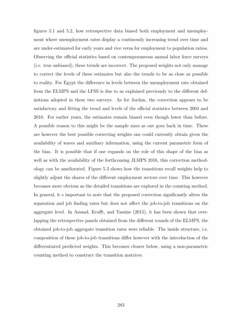
figures 5.1 and 5.2, how retrospective data biased both employment and unemploy-

ment where unemployment rates display a continously increasing trend over time and

are under-estimated for early years and vice versa for employment to population ratios.

Observing the official statistics based on contemporaneous annual labor force surveys

(i.e. true unbiased), these trends are incorrect. The proposed weights not only manage

to correct the levels of these estimates but also the trends to be as close as possible

to reality. For Egypt the difference in levels between the unemployment rate obtained

from the ELMPS and the LFSS is due to as explained previously to the different def-

initions adopted in these two surveys. As for Jordan, the correction appears to be

satisfactory and fitting the trend and levels of the official statistics between 2004 and

2010. For earlier years, the estimates remain biased even though lower than before.

A possible reason to this might be the sample sizes as one goes back in time. These

are however the best possible correcting weights one could currently obtain given the

availability of waves and auxiliary information, using the current parametric form of

the bias. It is possible that if one expands on the role of this shape of the bias as

well as with the availability of the forthcoming JLMPS 2016, this correction method-

ology can be ameliorated. Figure 5.3 shows how the transitions recall weights help to

slightly adjust the shares of the different employment sectors over time. This however

becomes more obvious as the detailed transitions are explored in the counting method.

In general, it s important to note that the proposed correction significantly alters the

separation and job finding rates but does not affect the job-to-job transitions on the

aggregate level. In Assaad, Krafft, and Yassine (2015), it has been shown that over-

lapping the retrospective panels obtained from the different rounds of the ELMPS, the

obtained job-to-job aggregate transition rates were reliable. The inside structure, i.e.

composition of these job-to-job transitions differ however with the introduction of the

differentiated predicted weights. This becomes clearer below, using a non-parametric

counting method to construct the transition matrices.

283

.02

.04

.06

.08

2000 2002 2004 2006 2008 2010

Unemp rate (raw) Unemp rate (corrected)

National estimate of unemp rate (CAPMAS)

(a) Egypt

.02

.04

.06

.08

.1

.12

.14

2000 2002 2004 2006 2008 2010

Unemp rate (raw) Unemp rate (corrected)

National estimate of unemp rate

(b) Jordan

Source: Author’s own calculations from ELMPS 2012, JLMPS2010, LFSS 2001-2011 and EUS 2000-2010.

Figure 5.1: Evolution of official, corrected and uncorrected unemployment rate overtime, Egypt 2001-2011 and Jordan 2000-2010, male workers, 15-49 years of age.

.65

.7.7

5.8

2000 2002 2004 2006 2008 2010

Emp/Pop ratio (raw) Emp/Pop ratio (corrected)

National estimate of emp/pop ratio (CAPMAS)

(a) Egypt

.55

.6.6

5.7

.75

2000 2002 2004 2006 2008 2010

Emp/Pop ratio (raw) Emp/Pop ratio (weighted)

National estimate of emp/pop ratio

(b) Jordan

Source: Author’s own calculations from ELMPS 2012, JLMPS2010, LFSS 2001-2011 (CAPMAS) and EUS 2000-2010 (DOS).

Figure 5.2: Evolution of official, corrected and uncorrected employment to populationratio over time, Egypt 2001-2011 and Jordan 2000-2010, male workers, 15-49 years ofage.

.1.2

.3.4

2001 2002 2004 2006 2008 2010year

Private Formal Wage Work (weighted) Private Informal Wage Work (weighted)

Public Sector (weighted) Non−wage work (weighted)

Private Formal Wage Work (raw) Private Informal Wage Work (raw)

Public Sector (raw) Non−wage work (raw)

(a) Egypt

.15

.2.2

5.3

.35

2000 2002 2004 2006 2008 2010year

Private Formal Wage Work (weighted) Private Informal Wage Work (weighted)

Public Sector (weighted) Non−wage work (weighted)

Private Formal Wage Work (raw) Private Informal Wage Work (raw)

Public Sector (raw) Non−wage work (raw)

(b) Jordan

Source: Author’s own calculations from ELMPS 2012, JLMPS2010, LFSS 2001-2011 (CAPMAS) and EUS 2000-2010 (DOS).

Figure 5.3: Evolution of corrected and uncorrected employment sectors’ shares in themarket over time, Egypt 2001-2011 and Jordan 2000-2010, male workers, 15-49 yearsof age.

284

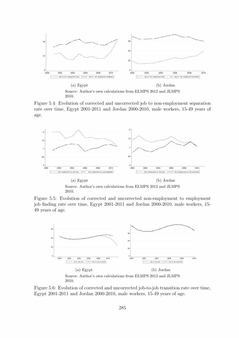
0

.01

.02

2000 2002 2004 2006 2008 2010

Job−to−non−employment (raw) Job−to− non−employment (weighted)

(a) Egypt

0

.02

.04

.06

2000 2002 2004 2006 2008 2010

Job−to−non−employment (raw) Job−to− non−employment (corrected)

(b) Jordan

Source: Author’s own calculations from ELMPS 2012 and JLMPS2010.

Figure 5.4: Evolution of corrected and uncorrected job to non-employment separationrate over time, Egypt 2001-2011 and Jordan 2000-2010, male workers, 15-49 years ofage.

0

.05

.1

.15

.2

2000 2002 2004 2006 2008 2010

Non−employment−to−Job (raw) Non−employment−to−Job (weighted)

(a) Egypt

0

.05

.1

.15

.2

2000 2002 2004 2006 2008 2010

Non−employment−to−Job (raw) Non−employment−to−Job (corrected)

(b) Jordan

Source: Author’s own calculations from ELMPS 2012 and JLMPS2010.

Figure 5.5: Evolution of corrected and uncorrected non-employment to employmentjob finding rate over time, Egypt 2001-2011 and Jordan 2000-2010, male workers, 15-49 years of age.

0

.02

.04

.06

2000 2002 2004 2006 2008 2010

Job−to−Job (raw) Job−to−Job (corrected)

(a) Egypt

0

.02

.04

.06

2000 2002 2004 2006 2008 2010

Job−to−Job (raw) Job−to−Job (corrected)

(b) Jordan

Source: Author’s own calculations from ELMPS 2012 and JLMPS2010.

Figure 5.6: Evolution of corrected and uncorrected job-to-job transition rate over time,Egypt 2001-2011 and Jordan 2000-2010, male workers, 15-49 years of age.

285

5.3.2 Counting

In this section, to be able to point out changes in the samples and their structure

as the recall weights are introduced, average transition probabilities between labor

market states are claculated via a simple non-parametric counting method. All types

of annual transitions are pooled over the constructed longitudinal panel of 10 years for

each country. An individual can therefore for example be at time t in one of five states

namely public wage work, private formal wage work, private informal wage work, self-

employment and non-employment. An individual can contribute up to 10 transitions

(over 10 years). It’s important to note that an individual who has reported being in the

public sector for the 10 years contribute to 10 transitions of type Public→ Public. The

same methodology applies when transitions are being considered between employment,

unemployment and inactivity, except that I choose to differentiate in that case between

individuals staying in the same job (SJ) and those who move to another job (JJ). This

distinction is interesting in how its estimates might be suggestive of how mobile the

labor market in question is.

The tables 5.1-5.4 group these transitions (obtained from raw data) by gender for

Egypt and Jordan. For males, these transitions are re-tabulated with both proportional

and predicted transition recall weights, to point out the difference and the advantage

of using a characteristics-specific weighting method. The realization of a particular

transition as follows. Given a random variable of a labor market state realization

at time t as Y (t) where the realizations of this variable is y(t) ∈ 1, 2, 3, 4, 5. The

realization of a particular transition from state l to state k is therefore defined as

follows:

Nlk = ΣNi=1ΣT

t=0I(yi(t) = k, yi(t− 1) = l) (5.28)

where i counts for all individuals and t counts for the time periods over the 10 year

panel specific for each country. yi(t) is therefore the realization of the labor market

state of individual i in year t. The average transition probability is then calculated

over the 10 year panel from state l to state k as Plk as follows:

286

Plk(t) = P (Yt = k|Yt−1 = l) =Nlk

ΣNi=1ΣT

t=0I(yi(t− 1) = l)(5.29)

For each country these transitions are first reported for the total sample as well as

for males and females in both transition probabilities and actual frequencies (expanded

counts). The labor market states defined in this analysis are public wage (G) work,

private formal wage work (F), private informal wage work (I), self-employment (NW)

and non-employment (NE). Aggregated labor market states are classified as follows:

Employed(E), Unemployed (U) and Out of Labor Force (O).

In order to make the paper reader friendly and to the point, the analysis is divided

below into two main comparisons: (i) comparisons between gender-specific transitions

and (ii) camparisons between the estimated transitions before and after correcting the

bias.

1. Males Versus Females:

In both countries, job-to-job transitions rate is higher for male than for female workers.

Given that the latter stay for a shorter period in the labor market and are more likely

to exit faster, they do not experience a lot of movements from one job to another.

Another possible explanation would be since its already more difficult for females to

find a job than males (job finding probability whether from unemployment or inactivity

is much lower for females in both Egypt and Jordan), it’s very unlikely that a female

worker would still for another job if she has got already one. Yassine (2015) shows that

in Egypt almost 80% of the job transitions are voluntary.

Both countries share a much higher job exit probability for females than for males.

Intuitively, these are more likely females exiting the labor market i.e. moving to inac-

tivity most likely after getting married or child birth. This becomes clarified and sup-

ported as one goes through the multinomial regressions’ estimations below. Two rates

strongly support this argument, the females’ formal sector separation rate (F–>NE)

and the females’ informal sector separation rates (I–>NE). These rates are strikingly

high and show how the private sector does not provide a flexible program in terms of

working hours, vacations..etc as the public sector

287

Going through the more detailed transitions, unsurprisingly the females highest job

finding rates are transitions towards the public sector. The public sector provides a

stable flexible job position for a female in the MENA region . Females in Jordan however

seem to access jobs in the formal private sector much easier than their Egyptian peers

though. In Egypt, evidence about the informal private sector being at a second resort

after the public is noted.

Discussing employment dynamics in general, the Jordanian labor market is more

mobile than the Egyptian labor market with much more churning as in higher job-to-

job transition rates and higher separation rates. However the Jordanian labor market

is much more segmented; inter-sectorial transitions for instance between the formal

private and informal private wage work is much lower than in Egypt. A possible ex-

planation to this might be the fact that Jordan has introduced flexibility in terms of

contracts and employers’ rights to laying off workers much earlier than Egypt. On the

one had, this tends to boost mobility in the labor market pushing to more high pro-

ductivity jobs being created and more low-productivity jobs beng destroyed. Moreover,

this flexibility scales down the difference between the formal and informal sector which

is clear in the Jordanian case. Not only that the size of the informal sector is lower than

the Egyptian labor market but the transitions between these sectors are minimized.

2. Adding transitions recall weights:

In general adding the transition recall weights corrects the over-estimated job find-

ing rates and the under-estimated separation rates. Using proportional or predicted

weights does not make a difference when correcting aggregated labor market transitions

i.e. between the states E, U and O12. However, it is obvious how the detailed labor mar-

ket transitions are modified once we introduce the predicted transition recall weights.

This shows that these weights do make a difference and emphasize the importance of

characterizing these weights according to the distribution of observed characteristics

among the transitions if one wants to characterize labor market flows later on or study

a more detailed level of transitions. Going back in time, the individuals who are more

12Expansion weights are re-scaled with the prediction weights in order to preserve the nationalrepresentativity of the sample.

288

probable to make a certain type of transition mis-report it, the structure and the char-

acteristics of the sample therefore get distorted. Since the retrospective samples are

in this case not random, adding the differentiated predicted weights, these samples

are redressed to become random, under the assumption that the determinants of the

probability of labor market transitions in the most recent year of the survey are the de-

terminants of mis-reporting back in time. The next section confirms how the predicted

recall weights are crucial if one needs to study labor market transitions by observable

characteristics.

289

Male

sF

emale

s

GF

IN

WN

ET

ota

lG

FI

NW

NE

Tota

lG

3.4

5E

+07

73136.2

592173.2

541416.8

4153018.3

3.4

9E

+07

G1.6

7E

+07

2.9

4E

+04

2.0

3E

+04

1.0

4E

+04

2.5

4E

+05

1.7

0E

+07

F181675.9

1.8

1E

+07

239673.1

215920

128636.5

1.8

9E

+07

F1.6

7E

+04

2.0

0E

+06

5.0

6E

+03

1.6

8E

+03

1.7

8E

+05

2.2

0E

+06

I559075

712592.3

5.9

3E

+07

673075.7

1009761

6.2

3E

+07

I3.1

4E

+04

2.7

1E

+04

4.0

7E

+06

3.9

7E

+04

5.5

8E

+05

4.7

2E

+06

NW

210394.9

151851.1

337294.7

3.4

3E

+07

275904.9

3.5

3E

+07

NW

5.9

1E

+03

0.0

0E

+00

2.1

8E

+04

1.0

2E

+07

1.7

6E

+05

1.0

4E

+07

NE

765374.2

866283.2

3484579

1121628

3.6

6E

+07

4.2

8E

+07

NE

1.0

3E

+06

3.0

1E

+05

6.4

0E

+05

4.9

3E

+05

1.6

2E

+08

1.6

4E

+08

Tota

l3.6

2E

+07

1.9

9E

+07

6.3

5E

+07

3.6

4E

+07

3.8

2E

+07

1.9

4E

+08

Tota

l1.7

8E

+07

2.3

6E

+06

4.7

6E

+06

1.0

7E

+07

1.6

3E

+08

1.9

9E

+08

EU

OT

ota

lE

UO

Tota

lE

1.5

0E

+08

500631.5

1066689

1.5

2E

+08

E3.3

3E

+07

257071.9

908325.6

3.4

5E

+07

U1446242

4259803

66169.3

95.7

7E

+06

U675243.7

9686185

16712.4

51.0

4E

+07

O4791622

1160618

3.1

1E

+07

3.7

1E

+07

O1785958

1278017

1.5

1E

+08

1.5

4E

+08

Tota

l1.5

6E

+08

5.9

2E

+06

3.2

2E

+07

1.9

4E

+08

Tota

l3.5

8E

+07

1.1

2E

+07

1.5

2E

+08

1.9

9E

+08

sam

ejo

bnew

job

NE

Tota

lsa

me

job

new

job

NE

Tota

lE

1.4

4E

+08

6050821

1567321

1.5

2E

+08

E3.2

7E

+07

565217.8

1165397

3.4

5E

+07

NE

6237864

3.6

6E

+07

4.2

8E

+07

NE

2461202

1.6

2E

+08

1.6

4E

+08

Tota

l1.5

6E

+08

38167321

1.9

4E

+08

Tota

l3.5

8E

+07

163165397

1.9

9E

+08

Male

s(%

)F

emale

s(%

)

GF

IN

WN

ET

ota

lG

FI

NW

NE

Tota

lG

98.9

7%

0.2

1%

0.2

6%

0.1

2%

0.4

4%

100.0

0%

G98.1

5%

0.1

7%

0.1

2%

0.0

6%

1.4

9%

100.0

0%

F0.9

6%

95.9

4%

1.2

7%

1.1

4%

0.6

8%

100.0

0%

F0.7

6%

90.8

7%

0.2

3%

0.0

8%

8.0

6%

100.0

0%

I0.9

0%

1.1

4%

95.2

5%

1.0

8%

1.6

2%

100.0

0%

I0.6

6%

0.5

7%

86.1

2%

0.8

4%

11.8

0%

100.0

0%

NW

0.6

0%

0.4

3%

0.9

6%

97.2

3%

0.7

8%

100.0

0%

NW

0.0

6%

0.0

0%

0.2

1%

98.0

4%

1.7

0%

100.0

0%

NE

1.7

9%

2.0

2%

8.1

3%

2.6

2%

85.4

4%

100.0

0%

NE

0.6

2%

0.1

8%

0.3

9%

0.3

0%

98.5

0%

100.0

0%

Tota

l18.6

6%

10.2

5%

32.6

9%

18.7

3%

19.6

6%

100.0

0%

Tota

l8.9

4%

1.1

9%

2.3

9%

5.4

0%

82.0

7%

100.0

0%

EU

OT

ota

lE

UO

Tota

lE

98.9

7%

0.3

3%

0.7

0%

100.0

0%

E96.6

2%

0.7

5%

2.6

4%

100.0

0%

U25.0

6%

73.8

0%

1.1

5%

100.0

0%

U6.5

1%

93.3

3%

0.1

6%

100.0

0%

O12.9

3%

3.1

3%

83.9

4%

100.0

0%

O1.1

6%

0.8

3%

98.0

1%

100.0

0%

Tota

l80.3

7%

3.0

5%

16.5

8%

100.0

0%

Tota

l17.9

8%

5.6

4%

76.3

8%

100.0

0%

sam

ejo

bnew

job

NE

Tota

lsa

me

job

new

job

NE

Tota

lE

94.9

7%

3.9

9%

1.0

3%

100.0

0%

E94.9

8%

1.6

4%

3.3

8%

100.0

0%

NE

14.5

6%

85.4

4%

100.0

0%

NE

1.5

0%

98.5

0%

100.0

0%

Tota

l80.3

7%

19.6

3%

100.0

0%

Tota

l17.9

8%

82.0

2%

100.0

0%

Tab

le5.

1:C

ount

ofL

abor

Mar

ket

Tra

nsi

tion

Pro

bab

ilit

ies

(obta

ined

from

raw

dat

a-

EL

MP

S20

12),

Mal

ean

dF

emal

ew

orke

rs,

Age

s15

-49

year

sol

d,

Egy

pt

2001

-201

1

290

Pre

dic

ted

Pro

port

ional

Wei

ghts

Wei

ghts

GF

IN

WN

ET

ota

lG

FI

NW

NE

Tota

lG

3.5

0E

+07

38952.0

75.0

6E

+04

17257.2

392075.9

93.5

2E

+07

G3.4

2E

+07

72485.3

691434.5

741067.4

2268685

3.4

7E

+07

F218926.5

1.7

7E

+07

239669.3

1.9

3E

+05

2.6

3E

+05

1.8

6E

+07

F180231.9

1.7

9E

+07

237755.7

214098.8

233337.1

1.8

8E

+07

I6.2

0E

+05

856441.4

5.8

2E

+07

623274.4

2051949

6.2

4E

+07

I554438

706544.5

5.8

8E

+07

667504.6

1786911

6.2

5E

+07

NW

182146.9

1.4

1E

+05

2.9

3E

+05

3.4

1E

+07

351098.4

3.5

1E

+07

NW

208637

150487.1

334348.1

3.4

0E

+07

469233.4

3.5

2E

+07

NE

676054.4

719916.3

2316746

756191.4

3.8

3E

+07

4.2

8E

+07

NE

552968.7

617960

2495886

802093.7

3.8

3E

+07

4.2

8E

+07

Tota

l3.6

7E

+07

1.9

5E

+07

6.1

1E

+07

3.5

7E

+07

4.1

1E

+07

1.9

4E

+08

Tota

l3.5

7E

+07

1.9

4E

+07

6.2

0E

+07

3.5

7E

+07

4.1

1E

+07

1.9

4E

+08

EU

OT

ota

lE

UO

Tota

lE

1.4

8E

+08

1149816

1608351

1.5

1E

+08

E1.4

8E

+08

1149816

1608351

1.5

1E

+08

U1172505

4483965

45109.1

25.7

0E

+06

U1172505

4483965

45109.1

25.7

0E

+06

O3296403

1156815

3.2

6E

+07

3.7

1E

+07

O3296403

1156815

3.2

6E

+07

3.7

1E

+07

Tota

l1.5

2E

+08

6.7

9E

+06

3.4

3E

+07

1.9

4E

+08

Tota

l1.5

2E

+08

6.7

9E

+06

3.4

3E

+07

1.9

4E

+08

sam

ejo

bnew

job

NE

Tota

lsa

me

job

new

job

NE

Tota

lE

1.4

2E

+08

5999967

2758167

1.5

1E

+08

E1.4

2E

+08

5999967

2758167

1.5

1E

+08

NE

4468908

3.8

3E

+07

4.2

8E

+07

NE

4468908

3.8

3E

+07

4.2

8E

+07

Tota

l1.5

2E

+08

41058167

1.9

4E

+08

Tota

l1.5

2E

+08

41058167

1.9

4E

+08

Pre

dic

ted

Pro

port

ional

Wei

ghts

(%)

Wei

ghts

(%)

GF

IN

WN

ET

ota

lG

FI

NW

NE

Tota

lG

99.4

3%

0.1

1%

0.1

4%

0.0

5%

0.2

6%

100.0

0%

G98.6

3%

0.2

1%

0.2

6%

0.1

2%

0.7

7%

100.0

0%

F1.1

8%

95.0

9%

1.2

9%

1.0

4%

1.4

1%

100.0

0%

F0.9

6%

95.3

9%

1.2

7%

1.1

4%

1.2

4%

100.0

0%

I0.9

9%

1.3

7%

93.3

4%

1.0

0%

3.2

9%

100.0

0%

I0.8

9%

1.1

3%

94.0

6%

1.0

7%

2.8

6%

100.0

0%

NW

0.5

2%

0.4

0%

0.8

4%

97.2

4%

1.0

0%

100.0

0%

NW

0.5

9%

0.4

3%

0.9

5%

96.6

9%

1.3

3%

100.0

0%

NE

1.5

8%

1.6

8%

5.4

2%

1.7

7%

89.5

5%

100.0

0%

NE

1.2

9%

1.4

4%

5.8

4%

1.8

8%

89.5

5%

100.0

0%

Tota

l18.9

2%

10.0

3%

31.4

9%

18.4

0%

21.1

6%

100.0

0%

Tota

l18.4

1%

10.0

3%

31.9

6%

18.4

3%

21.1

8%

100.0

0%

EU

OT

ota

lE

UO

Tota

lE

98.1

7%

0.7

6%

1.0

7%

100.0

0%

E98.1

7%

0.7

6%

1.0

7%

100.0

0%

U20.5

6%

78.6

4%

0.7

9%

100.0

0%

U20.5

6%

78.6

4%

0.7

9%

100.0

0%

O8.9

0%

3.1

2%

87.9

8%

100.0

0%

O8.9

0%

3.1

2%

87.9

8%

100.0

0%

Tota

l78.7

9%

3.5

1%

17.7

0%

100.0

0%

Tota

l78.7

9%

3.5

1%

17.7

0%

100.0

0%

sam

ejo

bnew

job

NE

Tota

lsa

me

job

new

job

NE

Tota

lE

94.1

9%

3.9

8%

1.8

3%

100.0

0%

E94.1

9%

3.9

8%

1.8

3%

100.0

0%

NE

10.4

5%

89.5

5%

100.0

0%

NE

10.4

5%

89.5

5%

100.0

0%

Tota

l78.7

8%

21.2

2%

100.0

0%

Tota

l78.7

8%

21.2

2%

100.0

0%

Tab

le5.

2:C

ount

ofL

abor

Mar

ket

Tra

nsi

tion

Pro

bab

ilit

ies

(obta

ined

from

corr

ecte

dw

eigh

ted

dat

a-

EL

MP

S20

12),

Mal

ew

orke

rs,

Age

s15

-49

year

sol

d,

Egy

pt

2001

-201

1

291

Male

sF

emale

s

GF

IN

WN

ET

ota

lG

FI

NW

NE

Tota

lG

3074467

19899.6

921188.6

21172.8

469435.2

43.2

1E

+06

G789017.7

1841.3

63

2739.7

65

194.4

097

29388.2

78.2

3E

+05

F57645.7

1725089

6716.8

38

4275.6

42

26166.5

71.8

2E

+06

F11969.9

6460233.2

1606.8

58

033037.7

35.0

7E

+05

I7976.2

69

15226.0

42844811

79832.3

288348.9

63.0

4E

+06

I977.6

423

2601.7

78

324181.6

3393.2

48

55331.8

73.8

6E

+05

NW

18982.4

614066.9

435359.2

1671810

28391.7

61.7

7E

+06

NW

1178.6

08

512.3

67

2205.7

29

132473

7600.2

71

1.4

4E

+05

NE

159661.9

126229.2

182187.8

54693.8

13954051

4.4

8E

+06

NE

66082.1

973912.2

857439.9

117143.9

81.2

2E

+07

1.2

4E

+07

Tota

l3.3

2E

+06

1.9

0E

+06

3.0

9E

+06

1.8

3E

+06

4.1

7E

+06

1.4

3E

+07

Tota

l8.6

9E

+05

5.3

9E

+05

3.8

8E

+05

1.5

3E

+05

1.2

3E

+07

1.4

3E

+07

EU

OT

ota

lE

UO

Tota

lE

9618520

140610.4

71732.0

99.8

3E

+06

E1735127

25768.3

899589.7

61.8

6E

+06

U237352.8

526357.9

2115.2

17.6

6E

+05

U73816.8

7262359.8

2151.1

73.3

8E

+05

O285419.8

172624.7

3252953

3.7

1E

+06

O140761.5

102750.6

1.1

8E

+07

1.2

0E

+07

Tota

l1.0

1E

+07

8.4

0E

+05

3.3

3E

+06

1.4

3E

+07

Tota

l1.9

5E

+06

3.9

1E

+05

1.1

9E

+07

1.4

2E

+07

sam

ejo

bnew

job

NE

Tota

lsa

me

job

new

job

NE

Tota

lE

8.9

0E

+06

723167.1

212342.5

9.8

3E

+06

E1.6

4E

+06

94712.5

5125358.1

1.8

6E

+06

NE

522772.7

3.9

5E

+06

4.4

8E

+06

NE

214578.4

1.2

2E

+07

1.2

4E

+07

Tota

l1.0

1E

+07

4166393.5

1.4

3E

+07

Tota

l1.9

5E

+06

12325358.1

1.4

3E

+07

Male

s(%

)F

emale

s(%

)

GF

IN

WN

ET

ota

lG

FI

NW

NE

Tota

lG

95.8

9%

0.6

2%

0.6

6%

0.6

6%

2.1

7%

100.0

0%

G95.8

5%

0.2

2%

0.3

3%

0.0

2%

3.5

7%

100.0

0%

F3.1

7%

94.7

9%

0.3

7%

0.2

3%

1.4

4%

100.0

0%

F2.3

6%

90.8

0%

0.3

2%

0.0

0%

6.5

2%

100.0

0%

I0.2

6%

0.5

0%

93.7

0%

2.6

3%

2.9

1%

100.0

0%

I0.2

5%

0.6

7%

83.8

8%

0.8

8%

14.3

2%

100.0

0%

NW

1.0

7%

0.8

0%

2.0

0%

94.5

3%

1.6

1%

100.0

0%

NW

0.8

2%

0.3

6%

1.5

3%

92.0

1%

5.2

8%

100.0

0%

NE

3.5

7%

2.8

2%

4.0

7%

1.2

2%

88.3

2%

100.0

0%

NE

0.5

3%

0.6

0%

0.4

6%

0.1

4%

98.2

7%

100.0

0%

Tota

l23.2

0%

13.2

8%

21.6

0%

12.8

0%

29.1

2%

100.0

0%

Tota

l6.0

9%

3.7

8%

2.7

2%

1.0

7%

86.3

4%

100.0

0%

EU

OT

ota

lE

UO

Tota

lE

97.8

4%

1.4

3%

0.7

3%

100.0

0%

E93.2

6%

1.3

9%

5.3

5%

100.0

0%

U30.9

9%

68.7

3%

0.2

8%

100.0

0%

U21.8

2%

77.5

5%

0.6

4%

100.0

0%

O7.6

9%

4.6

5%

87.6

6%

100.0

0%

O1.1

7%

0.8

5%

97.9

8%

100.0

0%

Tota

l70.8

8%

5.8

7%

23.2

5%

100.0

0%

Tota

l13.6

9%

2.7

4%

83.5

7%

100.0

0%

sam

ejo

bnew

job

NE

Tota

lsa

me

job

new

job

NE

Tota

lE

90.4

8%

7.3

6%

2.1

6%

100.0

0%

E88.1

7%

5.0

9%

6.7

4%

100.0

0%

NE

11.6

8%

88.3

2%

100.0

0%

NE

1.7

3%

98.2

7%

100.0

0%

Tota

l70.8

8%

29.1

2%

100.0

0%

Tota

l13.6

6%

86.3

4%

100.0

0%

Tab

le5.

3:C

ount

ofL

abor

Mar

ket

Tra

nsi

tion

Pro

bab

ilit

ies

(obta

ined

from

raw

-JL

MP

S20

10),

Mal

ean

dF

emal

ew

orke

rs,

Age

s15

-49

year

sol

d,

Jor

dan

2000

-201

0

292

Pre

dic

ted

Pro

port

ional

Wei

ghts

Wei

ghts

GF

IN

WN

ET

ota

lG

FI

NW

NE

Tota

lG

3083520

6883.4

94

7979.1

21

7419.8

3189640

3.3

0E

+06

G2948064

19097.3

220335.0

120265.8

1206777

3.2

1E

+06

F78273.0

91639251

8912.4

64

5696.6

56

45374.4

61.7

8E

+06

F55326.6

11654437

6415.2

31

4077.9

98

74156.5

91.7

9E

+06

I8823.0

79

17414.7

32620413

78337.6

5296877

3.0

2E

+06

I7657.4

84

14530.6

32727062

76556.4

8237406.4

3.0

6E

+06

NW

15802.0

811148.1

929494.5

31602657

59344.2

91.7

2E

+06

NW

18191.7

713485.2

733948.6

61602575

72895.8

21.7

4E

+06

NE

131417.4

118343.4

146522.5

51074.2

64072086

4.5

2E

+06

NE

137517.4

108053.2

156032.2

45754.7

34072086

4.5

2E

+06

Tota

l3.3

2E

+06

1.7

9E

+06

2.8

1E

+06

1.7

5E

+06

4.6

6E

+06

1.4

3E

+07

Tota

l3.1

7E

+06

1.8

1E

+06

2.9

4E

+06

1.7

5E

+06

4.6

6E

+06

1.4

3E

+07

EU

OT

ota

lE

UO

Tota

lE

9222027

380089.9

211145.9

9.8

1E

+06

E9222027

380089.9

211145.9

9.8

1E

+06

U210814.6

541675.3

2146.9

38

7.5

5E

+05

U210814.6

541675.3

2146.9

38

7.5

5E

+05

O236542.9

177679.5

3350584

3.7

6E

+06

O236542.9

177679.4

3350584

3.7

6E

+06

Tota

l9.6

7E

+06

1.1

0E

+06

3.5

6E

+06

1.4

3E

+07

Tota

l9.6

7E

+06

1.1

0E

+06

3.5

6E

+06

1.4

3E

+07

sam

ejo

bnew

job

NE

Tota

lsa

me

job

new

job

NE

Tota

lE

8.5

3E

+06

693952.3

591235.8

9.8

1E

+06

E8.5

3E

+06

693952.3

591235.8

9.8

1E

+06

NE

447357.5

4.0

7E

+06

4.5

2E

+06

NE

447357.5

4.0

7E

+06

4.5

2E

+06

Tota

l9.6

7E

+06

4663321.8

1.4

3E

+07

Tota

l9.6

7E

+06

4663321.8

1.4

3E

+07

Pre

dic

ted

Pro

port

ional

Wei

ghts

(%)

Wei

ghts

(%)

GF

IN

WN

ET

ota

lG

FI

NW

NE

Tota

lG

93.5

7%

0.2

1%

0.2

4%

0.2

3%

5.7

5%

100.0

0%

G91.7

1%

0.5

9%

0.6

3%

0.6

3%

6.4

3%

100.0

0%

F4.4

0%

92.2

2%

0.5

0%

0.3

2%

2.5

5%

100.0

0%

F3.0

8%

92.2

0%

0.3

6%

0.2

3%

4.1

3%

100.0

0%

I0.2

9%

0.5

8%

86.7

2%

2.5

9%

9.8

2%

100.0

0%

I0.2

5%

0.4

7%

89.0

3%

2.5

0%

7.7

5%

100.0

0%

NW

0.9

2%

0.6

5%

1.7

2%

93.2

6%

3.4

5%

100.0

0%

NW

1.0

4%

0.7

7%

1.9

5%

92.0

4%

4.1

9%

100.0

0%

NE

2.9

1%

2.6

2%

3.2

4%

1.1

3%

90.1

0%

100.0

0%

NE

3.0

4%

2.3

9%

3.4

5%

1.0

1%

90.1

0%

100.0

0%

Tota

l23.1

5%

12.5

1%

19.6

3%

12.1

8%

32.5

4%

100.0

0%

Tota

l22.0

9%

12.6

3%

20.5

4%

12.2

0%

32.5

4%

100.0

0%

EU

OT

ota

lE

UO

Tota

lE

93.9

8%

3.8

7%

2.1

5%

100.0

0%

E93.9

8%

3.8

7%

2.1

5%

100.0

0%

U27.9

4%

71.7

8%

0.2

8%

100.0

0%

U27.9

4%

71.7

8%

0.2

8%

100.0

0%

O6.2

8%

4.7

2%

89.0

0%

100.0

0%

O6.2

8%

4.7

2%

89.0

0%

100.0

0%

Tota

l67.4

6%

7.6

7%

24.8

7%

100.0

0%

Tota

l67.4

6%

7.6

7%

24.8

7%

100.0

0%

sam

ejo

bnew

job

NE

Tota

lsa

me

job

new

job

NE

Tota

lE

86.9

0%

7.0

7%

6.0

2%

100.0

0%

E86.9

0%

7.0

7%

6.0

2%

100.0

0%

NE

9.9

0%

90.1

0%

100.0

0%

NE

9.9

0%

90.1

0%

100.0

0%

Tota

l67.4

6%

32.5

4%

100.0

0%

Tota

l67.4

6%

32.5

4%

100.0

0%

Tab

le5.

4:C

ount

ofL

abor

Mar

ket

Tra

nsi

tion

Pro

bab

ilit

ies

(obta

ined

from

corr

ecte

dw

eigh

ted

-JL

MP

S20

10),

Mal

ew

orke

rs,

Age

s15

-49

year

sol

d,

Jor

dan

2000

-201

0

293

5.4 Determinants of Labor Market Transitions in

Egypt and Jordan: An Application Using Tran-

sitions Weights

Why are the transitions’ recall weights important? As an application to the tran-

sitions’ recall weights, created in the previous section, this paper estimates the labor

market transition probabilities in the two MENA countries Egypt and Jordan as a

function of the workers’ and firms’ observable characteristics, with a focus on the em-

ployment dynamics. This section therefore aims mainly at estimating the turnover

patterns and at exploring differences in the mobility behaviour. Although, this can be

done empirically by duration models13, as will be done in the next section, it was sug-

gested previously by Royalty (1998) that the interpretation of the estimated coefficients

on event probabilities using discrete choice models is easier and the results are more

accessible to policymakers14. I therefore choose to estimate the transition probabilities

in this section using a multinomial logit (MNL) specification. The labor market transi-

tions are modeled as a function of individual, household and job characteristics. Tansel

and Ozdemir (2015) provided similar estimations of detailed sectorial transitions over a

six-year using the ELMPS 2006 and 2012. A lot of short term transitions can however

take place in between six years. Given the nature and type of data available for the

countries in question, this paper chooses to pool all annual transitions from year t to

year t+ 1 over a period of 10 years, for each country, using the retrospective informa-

tion15. The methodology used in this section resembles that adopted by Theodossiou

and Zangelidis (2009). They choose to focus on employment dynamics as in transitions

13It is intended to extend this work to estimate a multi-state multi-spell model using the proposedpanel weights to test for the duration dependence of the labor market transitions in these countries.

14A principle objective of this thesis in general is to address the importance of studying the dy-namism of the labor market to policymakers. It is aimed to be perceived as a guide in countries whereeven official statistics fail to provide indicators about the labor market basic transitions (job findingand separations). Looking through the labor market transitions not only delivers a thorough idea(more than stocks) about the labor market’s status quo but also gives hints on how to adjust stocksto targeted levels via flows going into and out of these stocks.

15An eventual test to the robustness of the proposed correction methodology and to compare tran-sitions probabilities and coefficients obtained from retrospective and contemporaneous panel datasets,is to re-run the MNL regressions for Egypt for transitions between 2005 and 2011 (i.e. the closest 6year period available from the retrospective data to the transitions discussed in Tansel and Ozdemir(2015).

294

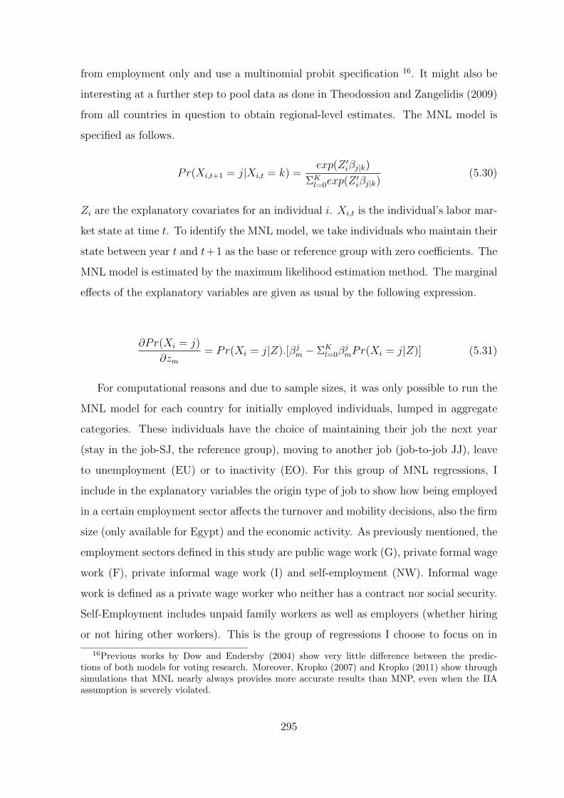
from employment only and use a multinomial probit specification 16. It might also be

interesting at a further step to pool data as done in Theodossiou and Zangelidis (2009)

from all countries in question to obtain regional-level estimates. The MNL model is

specified as follows.

Pr(Xi,t+1 = j|Xi,t = k) =exp(Z ′iβj|k)

ΣKl=0exp(Z

′iβj|k)

(5.30)

Zi are the explanatory covariates for an individual i. Xi,t is the individual’s labor mar-

ket state at time t. To identify the MNL model, we take individuals who maintain their

state between year t and t+1 as the base or reference group with zero coefficients. The

MNL model is estimated by the maximum likelihood estimation method. The marginal

effects of the explanatory variables are given as usual by the following expression.

∂Pr(Xi = j)

∂zm= Pr(Xi = j|Z).[βjm − ΣK

l=0βjmPr(Xi = j|Z)] (5.31)

For computational reasons and due to sample sizes, it was only possible to run the

MNL model for each country for initially employed individuals, lumped in aggregate

categories. These individuals have the choice of maintaining their job the next year

(stay in the job-SJ, the reference group), moving to another job (job-to-job JJ), leave

to unemployment (EU) or to inactivity (EO). For this group of MNL regressions, I

include in the explanatory variables the origin type of job to show how being employed

in a certain employment sector affects the turnover and mobility decisions, also the firm

size (only available for Egypt) and the economic activity. As previously mentioned, the

employment sectors defined in this study are public wage work (G), private formal wage

work (F), private informal wage work (I) and self-employment (NW). Informal wage

work is defined as a private wage worker who neither has a contract nor social security.

Self-Employment includes unpaid family workers as well as employers (whether hiring

or not hiring other workers). This is the group of regressions I choose to focus on in

16Previous works by Dow and Endersby (2004) show very little difference between the predic-tions of both models for voting research. Moreover, Kropko (2007) and Kropko (2011) show throughsimulations that MNL nearly always provides more accurate results than MNP, even when the IIAassumption is severely violated.

295

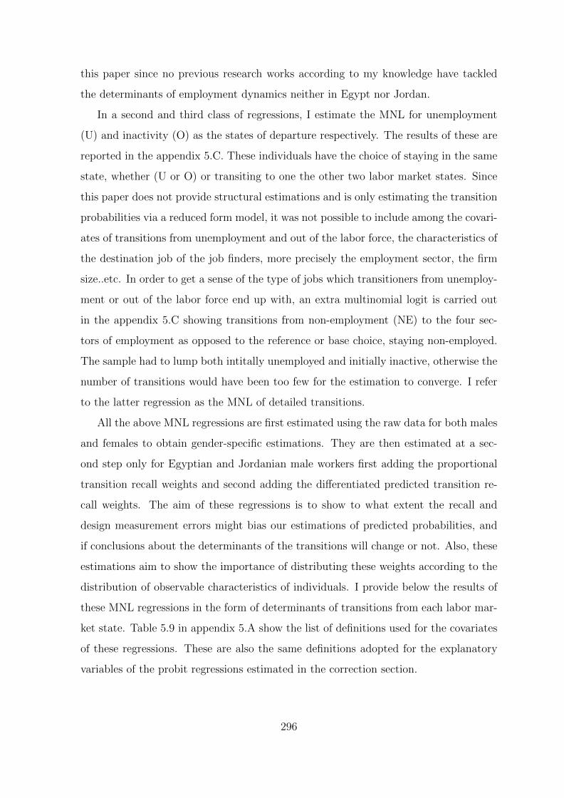
this paper since no previous research works according to my knowledge have tackled

the determinants of employment dynamics neither in Egypt nor Jordan.

In a second and third class of regressions, I estimate the MNL for unemployment

(U) and inactivity (O) as the states of departure respectively. The results of these are

reported in the appendix 5.C. These individuals have the choice of staying in the same

state, whether (U or O) or transiting to one the other two labor market states. Since

this paper does not provide structural estimations and is only estimating the transition

probabilities via a reduced form model, it was not possible to include among the covari-

ates of transitions from unemployment and out of the labor force, the characteristics of

the destination job of the job finders, more precisely the employment sector, the firm

size..etc. In order to get a sense of the type of jobs which transitioners from unemploy-

ment or out of the labor force end up with, an extra multinomial logit is carried out

in the appendix 5.C showing transitions from non-employment (NE) to the four sec-

tors of employment as opposed to the reference or base choice, staying non-employed.

The sample had to lump both intitally unemployed and initially inactive, otherwise the

number of transitions would have been too few for the estimation to converge. I refer

to the latter regression as the MNL of detailed transitions.

All the above MNL regressions are first estimated using the raw data for both males

and females to obtain gender-specific estimations. They are then estimated at a sec-

ond step only for Egyptian and Jordanian male workers first adding the proportional

transition recall weights and second adding the differentiated predicted transition re-

call weights. The aim of these regressions is to show to what extent the recall and

design measurement errors might bias our estimations of predicted probabilities, and

if conclusions about the determinants of the transitions will change or not. Also, these

estimations aim to show the importance of distributing these weights according to the

distribution of observable characteristics of individuals. I provide below the results of

these MNL regressions in the form of determinants of transitions from each labor mar-

ket state. Table 5.9 in appendix 5.A show the list of definitions used for the covariates

of these regressions. These are also the same definitions adopted for the explanatory

variables of the probit regressions estimated in the correction section.

296

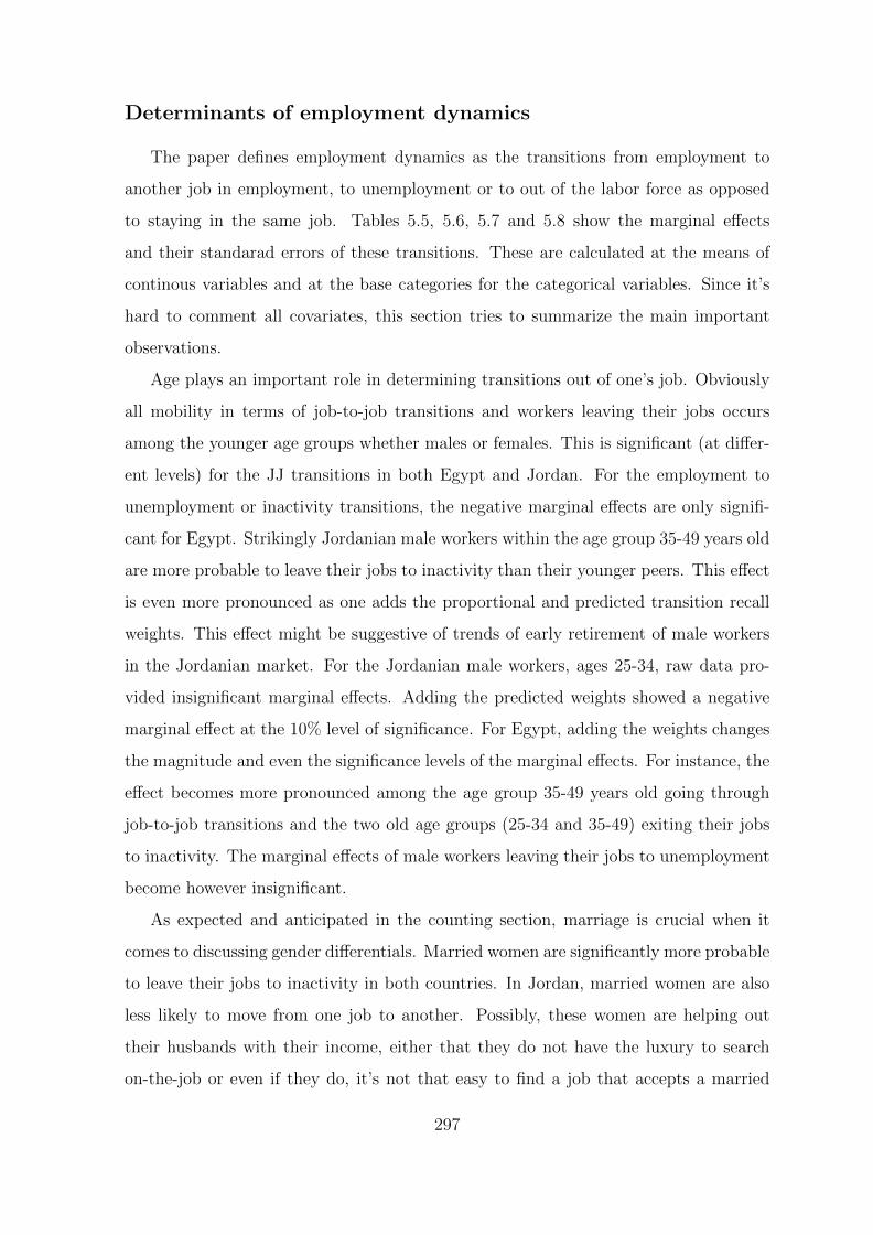
Determinants of employment dynamics

The paper defines employment dynamics as the transitions from employment to

another job in employment, to unemployment or to out of the labor force as opposed

to staying in the same job. Tables 5.5, 5.6, 5.7 and 5.8 show the marginal effects

and their standarad errors of these transitions. These are calculated at the means of

continous variables and at the base categories for the categorical variables. Since it’s

hard to comment all covariates, this section tries to summarize the main important

observations.

Age plays an important role in determining transitions out of one’s job. Obviously

all mobility in terms of job-to-job transitions and workers leaving their jobs occurs

among the younger age groups whether males or females. This is significant (at differ-

ent levels) for the JJ transitions in both Egypt and Jordan. For the employment to

unemployment or inactivity transitions, the negative marginal effects are only signifi-

cant for Egypt. Strikingly Jordanian male workers within the age group 35-49 years old

are more probable to leave their jobs to inactivity than their younger peers. This effect

is even more pronounced as one adds the proportional and predicted transition recall

weights. This effect might be suggestive of trends of early retirement of male workers

in the Jordanian market. For the Jordanian male workers, ages 25-34, raw data pro-

vided insignificant marginal effects. Adding the predicted weights showed a negative

marginal effect at the 10% level of significance. For Egypt, adding the weights changes

the magnitude and even the significance levels of the marginal effects. For instance, the

effect becomes more pronounced among the age group 35-49 years old going through

job-to-job transitions and the two old age groups (25-34 and 35-49) exiting their jobs

to inactivity. The marginal effects of male workers leaving their jobs to unemployment

become however insignificant.

As expected and anticipated in the counting section, marriage is crucial when it

comes to discussing gender differentials. Married women are significantly more probable

to leave their jobs to inactivity in both countries. In Jordan, married women are also

less likely to move from one job to another. Possibly, these women are helping out

their husbands with their income, either that they do not have the luxury to search

on-the-job or even if they do, it’s not that easy to find a job that accepts a married

297

woman with all potential maternity leaves and housework obligations. For men, it’s

the total opposite. In both countries, married men seems to be continously on the

move i.e. more probable to go through job-to-job transitions. This can be explained by

the fact that a married man is always looking for better jobs or maybe does not have

the luxury to stay unemployed or inactive if he leaves his job (whether voluntarily or

involuntarily). This is confirmed in both Egypt and Jordan, by the negative marginal

effects associated with the employment to unemployment and inactivity transitions of

married men. These effects are even more pronounced as one adds the transitions recall

weights in both countries especially the predicted weights.

Higher mobility patterns and job exits to unemployment are observed significantly

among the more educated groups of individuals for both males and females in Egypt. In

Jordan, these marginal effects are only significant for job-to-job transitions among male

university graduates and job to unemployment transitions among female university

graduates. Higher levels of education including intermediate and university levels also

lowers the probability that male workers exit the labor market (EO). In general the

effect of education gets more pronounced for Egypt as one adds the transition recall

weights. For Jordan, it becomes significantly less probable to exit the labor market as

a male university graduate. Also, literate males who do not have a formal education

are less probable to move from one job to another than their illiterate peers. This effect

becomes after being totally insignificant without weights to significant at the 10% level

after using weights.

One of the very interesting determinants providing common grounds between both

countries is the effect of time spent in the job before one transits to another job or

state. This provides an indication to the duration dependence, that will thoroughly be

examined through the next section. In both countries, the longer one stays in a job, the

less probable he/she leaves this job in search for another i.e. job-to-job transitioners.

This negative duration dependence is also significant for Egyptian workers moving to

unemployment and inactivity. It only becomes significant for the Jordanian workers as

the predicted transition recall weights are added to the estimation process.

Another major determinant of transitions in both countries is the type of employ-

ment occupied in the orgin status of the initially employed individuals. Intuitively,

298

higher job-to-job mobility patterns are observed among the private male wage and

non-wage workers than their peers employed in the public sector. This is also true for

the informal female wage workers. Evidence of higher probability to exits to unem-

ployment, in both countries among both males and females employed in the informal

sector. This reflects the instability and flexibility of this sector as opposed to its formal

counterpart. Confirming what has been previously discussed in the first non-parametric

section, females employed in the formal and informal private sector are generally more

likely to exit the labor market and become non-participants than when employed in

the public sector.

Having a child below the age of six revealed as an insignificant determinant of all

types of employment transitions except for the female jordanian workers. This is actu-

ally in line with what has been discussed previously in an unpublished manuscript by

Hendy (2012) that Egyptian females tend to have an unpaid work for family or become

self- employed after marriage and child birth contrarily to their Jordanian counterparts

who mostly become housewives. Interestingly, adding the predicted transition recall

weights reveals significant positive marginal effect of male workers having a child at

home to exit the labor market. This might be suggestive to male workers helping the

mothers of taking care of the children.

299

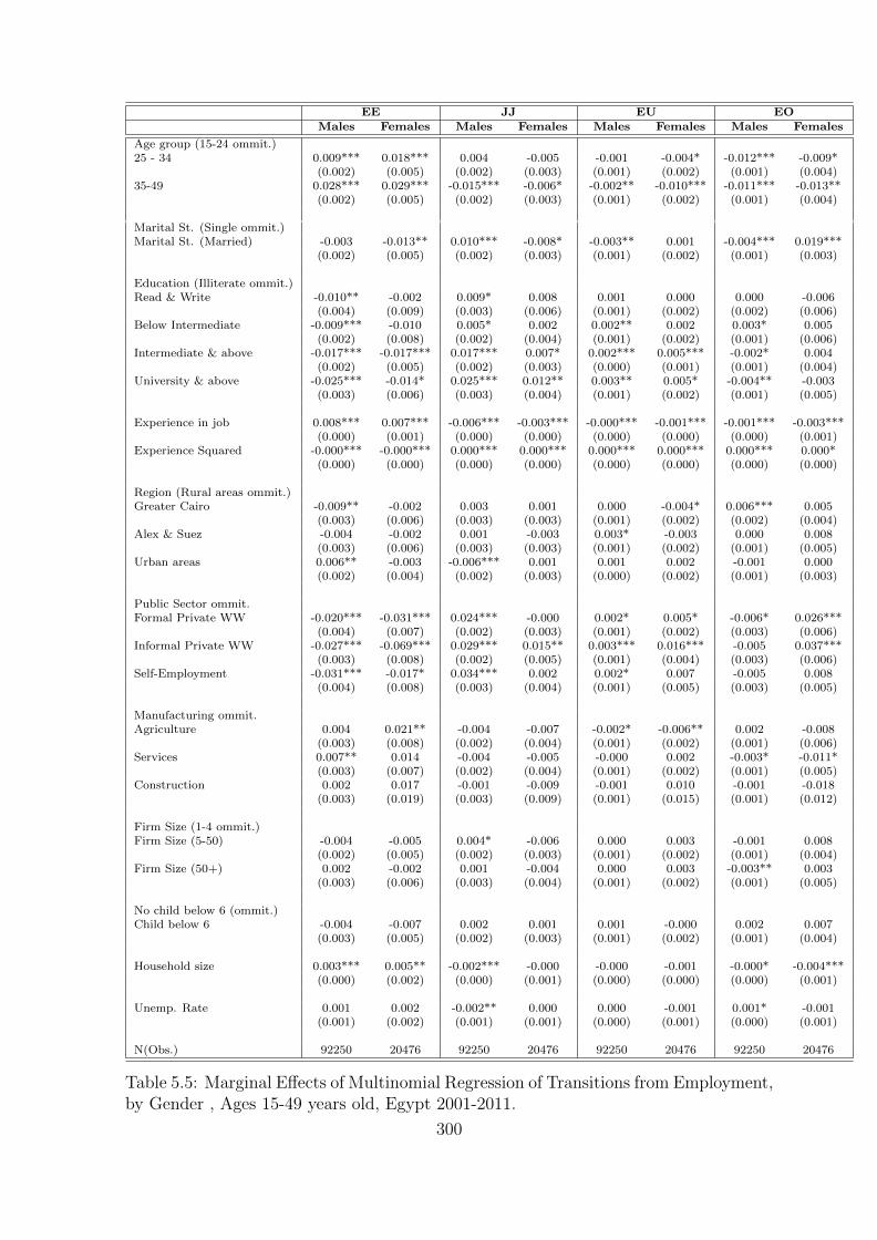
EE JJ EU EOMales Females Males Females Males Females Males Females

Age group (15-24 ommit.)25 - 34 0.009*** 0.018*** 0.004 -0.005 -0.001 -0.004* -0.012*** -0.009*

(0.002) (0.005) (0.002) (0.003) (0.001) (0.002) (0.001) (0.004)35-49 0.028*** 0.029*** -0.015*** -0.006* -0.002** -0.010*** -0.011*** -0.013**

(0.002) (0.005) (0.002) (0.003) (0.001) (0.002) (0.001) (0.004)

Marital St. (Single ommit.)Marital St. (Married) -0.003 -0.013** 0.010*** -0.008* -0.003** 0.001 -0.004*** 0.019***

(0.002) (0.005) (0.002) (0.003) (0.001) (0.002) (0.001) (0.003)

Education (Illiterate ommit.)Read & Write -0.010** -0.002 0.009* 0.008 0.001 0.000 0.000 -0.006

(0.004) (0.009) (0.003) (0.006) (0.001) (0.002) (0.002) (0.006)Below Intermediate -0.009*** -0.010 0.005* 0.002 0.002** 0.002 0.003* 0.005

(0.002) (0.008) (0.002) (0.004) (0.001) (0.002) (0.001) (0.006)Intermediate & above -0.017*** -0.017*** 0.017*** 0.007* 0.002*** 0.005*** -0.002* 0.004

(0.002) (0.005) (0.002) (0.003) (0.000) (0.001) (0.001) (0.004)University & above -0.025*** -0.014* 0.025*** 0.012** 0.003** 0.005* -0.004** -0.003

(0.003) (0.006) (0.003) (0.004) (0.001) (0.002) (0.001) (0.005)

Experience in job 0.008*** 0.007*** -0.006*** -0.003*** -0.000*** -0.001*** -0.001*** -0.003***(0.000) (0.001) (0.000) (0.000) (0.000) (0.000) (0.000) (0.001)

Experience Squared -0.000*** -0.000*** 0.000*** 0.000*** 0.000*** 0.000*** 0.000*** 0.000*(0.000) (0.000) (0.000) (0.000) (0.000) (0.000) (0.000) (0.000)

Region (Rural areas ommit.)Greater Cairo -0.009** -0.002 0.003 0.001 0.000 -0.004* 0.006*** 0.005

(0.003) (0.006) (0.003) (0.003) (0.001) (0.002) (0.002) (0.004)Alex & Suez -0.004 -0.002 0.001 -0.003 0.003* -0.003 0.000 0.008

(0.003) (0.006) (0.003) (0.003) (0.001) (0.002) (0.001) (0.005)Urban areas 0.006** -0.003 -0.006*** 0.001 0.001 0.002 -0.001 0.000

(0.002) (0.004) (0.002) (0.003) (0.000) (0.002) (0.001) (0.003)

Public Sector ommit.Formal Private WW -0.020*** -0.031*** 0.024*** -0.000 0.002* 0.005* -0.006* 0.026***

(0.004) (0.007) (0.002) (0.003) (0.001) (0.002) (0.003) (0.006)Informal Private WW -0.027*** -0.069*** 0.029*** 0.015** 0.003*** 0.016*** -0.005 0.037***

(0.003) (0.008) (0.002) (0.005) (0.001) (0.004) (0.003) (0.006)Self-Employment -0.031*** -0.017* 0.034*** 0.002 0.002* 0.007 -0.005 0.008

(0.004) (0.008) (0.003) (0.004) (0.001) (0.005) (0.003) (0.005)

Manufacturing ommit.Agriculture 0.004 0.021** -0.004 -0.007 -0.002* -0.006** 0.002 -0.008

(0.003) (0.008) (0.002) (0.004) (0.001) (0.002) (0.001) (0.006)Services 0.007** 0.014 -0.004 -0.005 -0.000 0.002 -0.003* -0.011*

(0.003) (0.007) (0.002) (0.004) (0.001) (0.002) (0.001) (0.005)Construction 0.002 0.017 -0.001 -0.009 -0.001 0.010 -0.001 -0.018

(0.003) (0.019) (0.003) (0.009) (0.001) (0.015) (0.001) (0.012)

Firm Size (1-4 ommit.)Firm Size (5-50) -0.004 -0.005 0.004* -0.006 0.000 0.003 -0.001 0.008

(0.002) (0.005) (0.002) (0.003) (0.001) (0.002) (0.001) (0.004)Firm Size (50+) 0.002 -0.002 0.001 -0.004 0.000 0.003 -0.003** 0.003

(0.003) (0.006) (0.003) (0.004) (0.001) (0.002) (0.001) (0.005)

No child below 6 (ommit.)Child below 6 -0.004 -0.007 0.002 0.001 0.001 -0.000 0.002 0.007

(0.003) (0.005) (0.002) (0.003) (0.001) (0.002) (0.001) (0.004)

Household size 0.003*** 0.005** -0.002*** -0.000 -0.000 -0.001 -0.000* -0.004***(0.000) (0.002) (0.000) (0.001) (0.000) (0.000) (0.000) (0.001)

Unemp. Rate 0.001 0.002 -0.002** 0.000 0.000 -0.001 0.001* -0.001(0.001) (0.002) (0.001) (0.001) (0.000) (0.001) (0.000) (0.001)

N(Obs.) 92250 20476 92250 20476 92250 20476 92250 20476

Table 5.5: Marginal Effects of Multinomial Regression of Transitions from Employment,by Gender , Ages 15-49 years old, Egypt 2001-2011.

300

EE

JJ

EU

EO

raw

prop

ortio

nal

predic

ted

raw

prop

ortio

nal

predic

ted

raw

prop

ortio

nal

predic

ted

raw

prop

ortio

nal

predic

ted

data

weig

hts

weig

hts

data

weig

hts

weig

hts

data

weig

hts

weig

hts

data

weig

hts

weig

hts

Agegro

up

(15-2

4ommit.)

25

-34

0.009***

0.017***

0.017***

0.004

0.004

0.001

-0.001

-0.004*

0.002

-0.012***

-0.018***

-0.020***

(0.002)

(0.003)

(0.003)

(0.002)

(0.002)

(0.002)

(0.001)

(0.001)

(0.002)

(0.001)

(0.001)

(0.001)

35-4

90.028***

0.035***

0.044***

-0.015***

-0.015***

-0.030***

-0.002**

-0.006**

0.004

-0.011***

-0.015***

-0.018***

(0.002)

(0.003)

(0.005)

(0.002)

(0.002)

(0.002)

(0.001)

(0.002)

(0.004)

(0.001)

(0.002)

(0.002)

Marita

lSt.

(Sin

gle

ommit.)

Marita

lSt.

(Married)

-0.003

-0.000

0.013*

0.010***

0.010***

0.015***

-0.003**

-0.005**

-0.017***

-0.004***

-0.005***

-0.011***

(0.002)

(0.003)

(0.005)

(0.002)

(0.002)

(0.002)

(0.001)

(0.002)

(0.005)

(0.001)

(0.001)

(0.002)

Education

(Illitera

teommit.)

Read

&W

rite

-0.010**

-0.009*

-0.013**

0.009*

0.008*

0.008**

0.001

0.001

0.002

0.000

-0.000

0.004

(0.004)

(0.004)

(0.004)

(0.003)

(0.003)

(0.003)

(0.001)

(0.002)

(0.001)

(0.002)

(0.003)

(0.004)

Below

Inte

rmediate

-0.009***

-0.012***

-0.015***

0.005*

0.005*

0.008***

0.002**

0.004*

0.005*

0.003*

0.003

0.003

(0.002)

(0.003)

(0.003)

(0.002)

(0.002)

(0.002)

(0.001)

(0.002)

(0.002)

(0.001)

(0.002)

(0.002)

Inte

rmediate

&above

-0.017***

-0.017***

-0.035***

0.017***

0.017***

0.031***

0.002***

0.003**

0.009***

-0.002*

-0.004**

-0.005**

(0.002)

(0.003)

(0.003)

(0.002)

(0.002)

(0.002)

(0.000)

(0.001)

(0.001)

(0.001)

(0.001)

(0.002)

University

&above

-0.025***

-0.024***

-0.038***

0.025***

0.025***

0.043***

0.003**

0.005*

0.006**

-0.004**

-0.006**

-0.011***

(0.003)

(0.004)

(0.004)

(0.003)

(0.003)

(0.003)

(0.001)

(0.002)

(0.002)

(0.001)

(0.002)

(0.002)

Experiencein

job

0.008***

0.009***

0.010***

-0.006***

-0.006***

-0.007***

-0.000***

-0.001***

-0.001***

-0.001***

-0.002***

-0.002***

(0.000)

(0.000)

(0.001)

(0.000)

(0.000)

(0.000)

(0.000)

(0.000)

(0.000)

(0.000)

(0.000)

(0.000)

ExperienceSquare

d-0

.000***

-0.000***

-0.000***

0.000***

0.000***

0.000***

0.000***

0.000***

0.000***

0.000***

0.000***

0.000***

(0.000)

(0.000)

(0.000)

(0.000)

(0.000)

(0.000)

(0.000)

(0.000)

(0.000)

(0.000)

(0.000)

(0.000)

Region

(Rura

lare

asommit.)

Gre

ate

rCairo

-0.009**

-0.012***

-0.033***

0.003

0.003

0.019***

0.000

0.001

0.007**

0.006***

0.008**

0.007*

(0.003)

(0.004)

(0.004)

(0.003)

(0.003)

(0.003)

(0.001)

(0.002)

(0.003)

(0.002)

(0.002)

(0.003)

Alex

&Suez

-0.004

-0.007

-0.008

0.001

0.001

0.003

0.003*

0.006**

0.012***

0.000

0.000

-0.007***

(0.003)

(0.004)

(0.004)

(0.003)

(0.003)

(0.003)

(0.001)

(0.002)

(0.004)

(0.001)

(0.002)

(0.001)

Urb

an

are

as

0.006**

0.004

0.007**

-0.006***

-0.006***

-0.007***

0.001

0.002

0.004**

-0.001

-0.000

-0.005***

(0.002)

(0.002)

(0.002)

(0.002)

(0.002)

(0.002)

(0.000)

(0.001)

(0.002)

(0.001)

(0.001)

(0.001)

PublicSecto

rommit.

Form

alPrivate

WW

-0.020***

-0.019***

-0.031***

0.024***

0.025***

0.031***

0.002*

0.003

0.006**

-0.006*

-0.008*

-0.006

(0.004)

(0.004)

(0.005)

(0.002)

(0.002)

(0.002)

(0.001)

(0.002)

(0.002)

(0.003)

(0.004)

(0.005)

Inform

alPrivate

WW

-0.027***

-0.028***

-0.050***

0.029***

0.029***

0.042***

0.003***

0.005**

0.010***

-0.005

-0.005

-0.002

(0.003)

(0.004)

(0.005)

(0.002)

(0.002)

(0.002)

(0.001)

(0.002)

(0.002)

(0.003)

(0.004)

(0.004)

Self-E

mployment

-0.031***

-0.031***

-0.037***

0.034***

0.033***

0.040***

0.002*

0.003

0.001*

-0.005

-0.006

-0.004

(0.004)

(0.005)

(0.005)

(0.003)

(0.003)

(0.003)

(0.001)

(0.002)

(0.001)

(0.003)

(0.004)

(0.004)

Manufactu

ring

ommit.

Agriculture

0.004

0.005

0.003

-0.004

-0.003

-0.005

-0.002*

-0.005**

-0.002

0.002

0.003

0.004

(0.003)

(0.003)

(0.004)

(0.002)

(0.002)

(0.003)

(0.001)

(0.002)

(0.003)

(0.001)

(0.002)

(0.002)

Serv

ices

0.007**

0.008**

0.003

-0.004

-0.004

-0.002

-0.000

-0.000

0.000

-0.003*

-0.004*

-0.001

(0.003)

(0.003)

(0.003)

(0.002)

(0.002)

(0.002)

(0.001)

(0.002)

(0.002)

(0.001)

(0.002)

(0.002)

Constru

ction

0.002

0.003

0.000

-0.001

-0.000

-0.000

-0.001

-0.001

-0.001

-0.001

-0.001

0.001

(0.003)

(0.004)

(0.004)

(0.003)

(0.003)

(0.003)

(0.001)

(0.002)

(0.003)

(0.001)

(0.002)

(0.002)

Firm

Size(1

-4ommit.)

Firm

Size(5

-50)

-0.004

-0.004

-0.004

0.004*

0.004*

0.004*

0.000

0.001

0.001

-0.001

-0.001

-0.001

(0.002)

(0.003)

(0.003)

(0.002)

(0.002)

(0.002)

(0.001)

(0.001)

(0.002)

(0.001)

(0.001)

(0.001)

Firm

Size(5

0+)

0.002

0.003

-0.003

0.001

0.001

0.004

0.000

0.000

0.004

-0.003**

-0.004*

-0.004

(0.003)

(0.004)

(0.004)

(0.003)

(0.003)

(0.003)

(0.001)

(0.002)

(0.003)

(0.001)

(0.002)

(0.002)

No

child

below

6(o

mmit.)

Child

below

6-0

.004

-0.005

-0.009**

0.002

0.002

0.005

0.001

0.001

0.002

0.002

0.002

0.002

(0.003)

(0.003)

(0.003)

(0.002)

(0.002)

(0.002)

(0.001)

(0.001)

(0.002)

(0.001)

(0.001)

(0.002)

House

hold

size

0.003***

0.003***

0.005***

-0.002***

-0.002***

-0.003***

-0.000

-0.000

-0.001

-0.000*

-0.001*

-0.001*

(0.000)

(0.001)

(0.001)

(0.000)

(0.000)

(0.001)

(0.000)

(0.000)

(0.001)

(0.000)

(0.000)

(0.000)

Unemp.Rate

0.001

0.002*

0.002*

-0.002**

-0.002**

-0.002**

0.000

-0.000

-0.000

0.001*

0.000

0.000

(0.001)

(0.001)

(0.001)

(0.001)

(0.001)

(0.001)

(0.000)

(0.000)

(0.001)

(0.000)

(0.000)

(0.000)

N(O

bs.)

92250

92250

92250

92250

92250

92250

92250

92250

92250

92250

92250

92250

Tab

le5.

6:M

argi

nal

Eff

ects

ofM

ult

inom

ial

Reg

ress

ion

ofT

ransi

tion

sfr

omE

mplo

ym

ent,

Mal

eW

orke

rs,

Age

s15

-49

year

sol

d,

Egy

pt

2001

-201

1.

301

EE JJ EU EO

Males Females Males Females Males Females Males FemalesAge group (15-24 ommit.)25 - 34 0.033*** 0.028 -0.031*** -0.014 -0.001 0.006 -0.001 -0.019

(0.006) (0.015) (0.005) (0.011) (0.002) (0.004) (0.002) (0.011)35-49 0.040*** 0.055*** -0.043*** -0.037** -0.002 -0.001 0.005* -0.017

(0.007) (0.016) (0.006) (0.011) (0.003) (0.004) (0.002) (0.012)

Marital St. (Single ommit.)Marital St. (Married) 0.010 -0.029** 0.010* -0.014 -0.012*** -0.000 -0.008** 0.044***

(0.006) (0.010) (0.004) (0.008) (0.003) (0.004) (0.003) (0.006)

Education (Illiterate ommit.)Read & Write 0.009 0.028 -0.003 -0.026 -0.002 0.001 -0.004 -0.003

(0.009) (0.028) (0.008) (0.017) (0.004) (0.006) (0.003) (0.021)Below Intermediate -0.004 -0.023 0.008 -0.015 0.001 0.010 -0.005 0.028

(0.008) (0.023) (0.007) (0.015) (0.004) (0.006) (0.003) (0.015)Intermediate & above -0.004 -0.015 0.008 -0.008 -0.001 0.005 -0.003 0.018

(0.009) (0.022) (0.007) (0.015) (0.004) (0.005) (0.003) (0.013)University & above -0.014 -0.015 0.022** 0.015 -0.003 0.014** -0.005 -0.014

(0.009) (0.023) (0.008) (0.015) (0.004) (0.005) (0.003) (0.013)

Experience in job 0.003** 0.008** -0.003*** -0.005** -0.000 -0.002 0.000* -0.002(0.001) (0.003) (0.001) (0.002) (0.000) (0.001) (0.000) (0.002)

Experience Squared -0.000*** -0.000** 0.000*** 0.000** 0.000*** 0.000 0.000 0.000*(0.000) (0.000) (0.000) (0.000) (0.000) (0.000) (0.000) (0.000)

Region (Middle ommit.)North -0.004 0.003 -0.002 -0.011 0.004* 0.008 0.002* -0.001

(0.004) (0.009) (0.003) (0.007) (0.002) (0.004) (0.001) (0.007)South 0.015** 0.043*** -0.015*** -0.015 0.002 -0.003 -0.002 -0.026***

(0.005) (0.011) (0.004) (0.008) (0.002) (0.004) (0.001) (0.007)

Public Sector ommit.Formal Private WW -0.060*** -0.060*** 0.064*** 0.028*** 0.002 0.015*** -0.006*** 0.016*

(0.005) (0.011) (0.005) (0.008) (0.002) (0.004) (0.001) (0.008)Informal Private WW -0.060*** -0.129*** 0.050*** 0.027** 0.009*** 0.030*** 0.000 0.071***

(0.005) (0.015) (0.004) (0.009) (0.002) (0.006) (0.001) (0.011)Self-Employment -0.025*** -0.034 0.027*** 0.023 0.002 0.005 -0.003* 0.006

(0.005) (0.018) (0.004) (0.014) (0.002) (0.005) (0.001) (0.010)

Manufacturing ommit.Agriculture -0.006 0.022 0.013 0.000 -0.004 -0.004 -0.003 -0.018

(0.008) (0.019) (0.008) (0.014) (0.003) (0.005) (0.002) (0.013)Services 0.004 -0.010 -0.006 0.016* 0.001 0.005 0.001 -0.011

(0.005) (0.012) (0.004) (0.008) (0.002) (0.004) (0.002) (0.009)Construction 0.003 0.019 -0.003 -0.025 0.001 0.013 -0.001 -0.007

(0.007) (0.037) (0.006) (0.014) (0.003) (0.019) (0.002) (0.028)

No child below 6 (ommit.)Child below 6 0.013 -0.022 -0.012 -0.001 -0.004 -0.004 0.003 0.028***

(0.007) (0.012) (0.007) (0.010) (0.004) (0.005) (0.002) (0.008)

Household size 0.001 0.008*** -0.002* -0.002 0.000 -0.002 0.000 -0.004*(0.001) (0.002) (0.001) (0.002) (0.000) (0.001) (0.000) (0.002)

Unemp. Rate 0.009*** 0.003 -0.006*** 0.002 -0.002*** -0.001 -0.000 -0.004*(0.001) (0.003) (0.001) (0.002) (0.000) (0.001) (0.000) (0.002)

N(Obs.) 41101 7801 41101 7801 41101 7801 41101 7801

Table 5.7: Marginal Effects of Multinomial Regression of Transitions from Employment,by Gender , Ages 15-49 years old, Jordan 2000-2010.

302

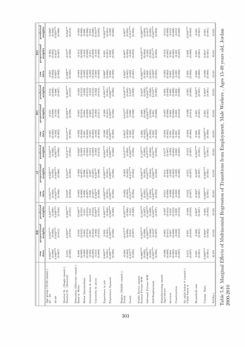
EE

JJ

EU

EO

raw

prop

ortio

nal

predic

ted

raw

prop

ortio

nal

predic

ted

raw

prop

ortio

nal

predic

ted

raw

prop

ortio

nal

predic

ted

data

weig

hts

weig

hts

data

weig

hts

weig

hts

data

weig

hts

weig

hts

data

weig

hts

weig

hts

Agegro

up

(15-2

4ommit.)

25

-34

0.033***

0.043***

0.037***

-0.031***

-0.028***

-0.043***

-0.001

-0.011

0.012

-0.001

-0.004

-0.006*

(0.006)

(0.009)

(0.008)

(0.005)

(0.005)

(0.006)

(0.002)

(0.008)

(0.006)

(0.002)

(0.005)

(0.003)

35-4

90.040***

0.042***

0.036***

-0.043***

-0.040***

-0.067***

-0.002

-0.016

0.006

0.005*

0.014*

0.025***

(0.007)

(0.011)

(0.010)

(0.006)

(0.006)

(0.006)

(0.003)

(0.009)

(0.007)

(0.002)

(0.007)

(0.006)

Marita

lSt.

(Sin

gle

ommit.)

Marita

lSt.

(Married)

0.010

0.029**

0.094***

0.010*

0.012**

0.014***

-0.012***

-0.023**

-0.064***

-0.008**

-0.017*

-0.044**

(0.006)

(0.010)

(0.015)

(0.004)

(0.004)

(0.004)

(0.003)

(0.008)

(0.010)

(0.003)

(0.008)

(0.014)

Education

(Illitera

teommit.)

Read

&W

rite

0.009

0.018

0.048**

-0.003

-0.002

-0.022*

-0.002

-0.001

-0.023

-0.004

-0.014

-0.003

(0.009)

(0.015)

(0.015)

(0.008)

(0.007)

(0.009)

(0.004)

(0.010)

(0.012)

(0.003)

(0.009)

(0.006)

Below

Inte

rmediate

-0.004

0.004

0.011

0.008

0.008

-0.014

0.001

0.004

-0.002

-0.005

-0.016

0.006

(0.008)

(0.014)

(0.014)

(0.007)

(0.007)

(0.009)

(0.004)

(0.009)

(0.012)

(0.003)

(0.009)

(0.006)

Inte

rmediate

&above

-0.004

0.001

0.015

0.008

0.007

-0.014

-0.001

0.003

-0.013

-0.003

-0.011

0.012

(0.009)

(0.014)

(0.014)

(0.007)

(0.007)

(0.009)

(0.004)

(0.010)

(0.012)

(0.003)

(0.009)

(0.006)

University

&above

-0.014

-0.002

0.040**

0.022**

0.021**

-0.003

-0.003

-0.003

-0.022

-0.005

-0.016

-0.015**

(0.009)

(0.015)

(0.015)

(0.008)

(0.008)

(0.010)

(0.004)

(0.011)

(0.013)

(0.003)

(0.009)

(0.005)

Experiencein

job

0.003**

0.002

0.005***

-0.003***

-0.003***

-0.004***

-0.000

-0.000

-0.005***

0.000*

0.001

0.003***

(0.001)

(0.001)

(0.002)

(0.001)

(0.001)

(0.001)

(0.000)

(0.001)

(0.001)

(0.000)

(0.001)

(0.001)

ExperienceSquare

d-0

.000***

-0.000***

-0.000***

0.000***

0.000***

0.000***

0.000***

0.000**

0.000***

0.000

0.000

-0.000

(0.000)

(0.000)

(0.000)

(0.000)

(0.000)

(0.000)

(0.000)

(0.000)

(0.000)

(0.000)

(0.000)

(0.000)

Region

(Mid

dle

ommit.)

North

-0.004

-0.017**

-0.037***

-0.002

-0.003

0.013***

0.004*

0.012**

0.018***

0.002*

0.007*

0.007*

(0.004)

(0.006)

(0.006)

(0.003)

(0.003)

(0.003)

(0.002)

(0.005)

(0.005)

(0.001)

(0.003)

(0.003)

South

0.015**

0.013

0.014

-0.015***

-0.014***

-0.022***

0.002

0.006

0.019*

-0.002

-0.005

-0.011***

(0.005)

(0.007)

(0.008)

(0.004)

(0.004)

(0.004)

(0.002)

(0.006)

(0.008)

(0.001)

(0.003)

(0.003)

PublicSecto

rommit.

Form

alPrivate

WW

-0.060***

-0.053***

-0.104***

0.064***

0.062***

0.123***

0.002

0.009

0.010*

-0.006***

-0.018***

-0.029***

(0.005)

(0.008)

(0.007)

(0.005)

(0.005)

(0.005)

(0.002)

(0.006)

(0.004)

(0.001)

(0.004)

(0.004)

Inform

alPrivate

WW

-0.060***

-0.069***

-0.120***

0.050***

0.047***

0.077***

0.009***

0.024***

0.054***

0.000

-0.003

-0.011*

(0.005)

(0.008)

(0.008)

(0.004)

(0.004)

(0.004)

(0.002)

(0.006)

(0.006)

(0.001)

(0.004)

(0.005)

Self-E

mployment

-0.025***

-0.016*

-0.033***

0.027***

0.026***

0.041***

0.002

0.001

0.018**

-0.003*

-0.011**

-0.027***

(0.005)

(0.007)

(0.007)

(0.004)

(0.004)

(0.003)

(0.002)

(0.006)

(0.006)

(0.001)

(0.004)

(0.004)

Manufactu

ring

ommit.

Agriculture

-0.006

0.003

-0.007

0.013

0.014

0.017*

-0.004

-0.007

0.004

-0.003

-0.010

-0.014

(0.008)

(0.011)

(0.014)

(0.008)

(0.008)

(0.007)

(0.003)

(0.008)

(0.009)

(0.002)

(0.005)

(0.009)

Serv

ices

0.004

0.001

0.010

-0.006

-0.005

-0.004

0.001

0.003

0.005

0.001

0.001

-0.012

(0.005)

(0.008)

(0.010)

(0.004)

(0.004)

(0.004)

(0.002)

(0.006)

(0.006)

(0.002)

(0.005)

(0.008)

Constru

ction

0.003

-0.000

0.009

-0.003

-0.003

0.000

0.001

0.005

0.004

-0.001

-0.001

-0.013

(0.007)

(0.013)

(0.012)

(0.006)

(0.006)

(0.005)

(0.003)

(0.010)

(0.008)

(0.002)

(0.007)

(0.009)

No

child

below

6(o

mmit.)

Child

below

60.013

0.021

-0.004

-0.012

-0.011

-0.013

-0.004

-0.020

-0.001

0.003

0.009

0.018***

(0.007)

(0.014)

(0.010)

(0.007)

(0.007)

(0.007)

(0.004)

(0.014)

(0.009)

(0.002)

(0.006)

(0.003)

House

hold

size

0.001

-0.000

0.003*

-0.002*

-0.002*

-0.004***

0.000

0.001

0.002**

0.000

0.001

-0.001

(0.001)

(0.001)

(0.001)

(0.001)

(0.001)

(0.001)

(0.000)

(0.001)

(0.001)

(0.000)

(0.001)

(0.001)

Unemp.Rate

0.009***

0.004*

0.003

-0.006***

-0.006***

-0.007***

-0.002***

0.001

0.003*

-0.000

0.001*

0.001

(0.001)

(0.002)

(0.002)

(0.001)

(0.001)

(0.001)

(0.000)

(0.001)

(0.001)

(0.000)

(0.001)

(0.001)

N(O

bs.)

41101

41101

41101

41101

41101

41101

41101

41101

41101

41101

41101

41101

Tab

le5.

8:M

argi

nal

Eff

ects

ofM

ult

inom

ialR

egre

ssio

nof

Tra

nsi

tion

sfr

omE

mplo

ym

ent,

Mal

eW

orke

rs,

Age

s15

-49

year

sol

d,

Jor

dan

2000

-201

0

303

5.5 Conclusion

Given that there are no official statistics on labor market dynamics in the MENA

region, as has been explained in parts I and II of this thesis, the only way to study

short-term labor market transitions in Egypt and Jordan is by extracting longitudinal

retrospective panels. These panels were shown to suffer from recall and design measure-

ment errors. This paper suggests a correction technique that shows that it is sufficient

to have population, stocks and transitions, moments to correct over- or under-reporting

biases in retrospective data. The true unbiased moments can be obtained from auxiliary

information such as contemporaneous information from other waves of the same survey,

or even external data sources, so long comparability between the varaibles’ definitions

is verified. Once the moments are matched on the aggregate level, a measurement error

for each type of transition at a point in time t can be estimated. This measurement er-

ror is then distributed among the sample’s individual observations/transactions in the

form of micro-data weights, such as observations that are being under-reported take

higher weights and those over-reported take lower weights. The paper proposes two

types of weights: (1)naive proportional weights and (2)differentiated predicted weights.

The paper shows significant different results as these weights are added showing how

crucial correcting recall and design measurement errors is to be able to obtain unbi-

ased estimations for labor market transition probabilities. These weights, especially

the differentiated predicted weights, make significant changes to the levels and compo-

sition of the labor market transitions obtained from the retrospective data since now

the samples are redressed to become random under the assumptions of the model. The

correction methodology proposed in this paper alters significant the rates of separations

and job findings in Egypt and Jordan which have been shown, in previous chapters, to

be under-estimated and over-estimated respectively.

The paper also shows the importance of these weights via an application by ex-

ploring the determinants of labor market transitions in general in two MENA region

countries, Egypt and Jordan. The methodology discussed explores in particular the

employment turnover patterns among the different groups of individuals in the market

as well as their job-to-job mobility behaviour. The analysis is also done, even though

304

for using uncorrected data, on a gender-specific basis to be able to make conclusions

about gender differentials in transitions.

The main findings of this paper show that Jordan has a much more mobile labor

market than that of Egypt. For both male and female workers, job-to-job transitions

rates and job to non-employment separation rates are higher. Age and gender play

important roles as determinants to job turnover and mobility in both markets. More

educated male workers are more mobile and prone to leaving to unemployment than

their less educated/illiterate peers, especially in Egypt. The public sector in both

countries is very stagnant as opposed to the private wage and non-wage employment.

Public wage workers tend to remain employed during their entire careeer and only leave

to inactivity as they wish to retire. The public sector also provides a flexible employer

for the female workers in both Egypt and Jordan otherwise these workers are found to

leave the labor market after their marriage or as they have a child (as in the case of

Jordan for instance). The significant effects of the type of employment in the origin job

are suggestive to the extent of state dependence of these labor market/state transitions.

Preliminary evidence from both the multinomial logit regressions and the non-

parametric survival analysis show obvious negative duration dependence of these em-

ployment transitions. In both countries, Egypt and Jordan, for male workers, employ-

ment to unemployment transitions appear to accelerate at the early years of a job and

then flatten out over time. The same pattern is observed for the job-to-job transitions,

however these transitions tend to decelerate a bit later than the job leaves. For the

Egyptian job to out of the labor force transitions, one observes a similar behavior to

that of the job to unemployment. However, for Jordan, the pattern is a bit surprising

where quits out of the labor market starts accelerating substantially between 10 years

after appointment up to around 25 years after appointment. Female workers exhibit

more or less similar patterns to those of the male workers except that they tend to

leave employment much earlier and their job-to-job transitions are much less probable.

Extensions: This paper is a preliminary milestone in a bigger project, where first

the correction methodology is aimed to be developped. Given the over-identification of

the model, tests of goodness of fit are required to prove how reliable the obtained esti-

mates are. Expanding on the role of the parametric form of the recall and design bias

305

is crucial to explore to what extent the obtained results rely on it. Among the applica-

tions of the weights, a multi-state multi-spell model is aimed to be built and estimated

for the transitions in Egypt and Jordan and estimated using panel weights. These panel

weights are also used in the next chapter (chapter 6) for the structural estimation of

the Burdett-Mortensen model using duration data from Egypt and Jordan. Finally,

cross-country comparisons are usually problematic if one ignores contextualizing the

analysis to the nature of the market and institutions of each country. A country where

flexible employment protection laws have been implemented long ago, such as Jordan,

would definitely be expected to be more flexible in terms of job-to-job transitions and

separations than another where short term contracts have just been introduced and

allowed in the market. In order to be able to conclude some policy implications for

each of the countries analyzed in this paper, the reduced form transitions estimated in

this paper serve as a tool for a further step which would be pluging these estimates into

a job search equilibrium model to simulate for the wage dispersion among the different

soci-economic groups, the different labor market policies and hence conclude robust

policy recommendations. These can also be compared to the results obtained from the

structural estimation of the job-search model in chapter 6. Combining these techniques,

where transition rates from state and duration dependence models are injected into a

job search equilibrium model to simulate for policy implications, is a novel technique

that according to my knowledge has not been previously adopted by the literature

and is worth exploring in a future research agenda. Usually these models are used for

simulations using a memoryless process such as poisson for the transitions.

306

References

Assaad, R. (2014): “The structure and evolution of employment in Jordan,” in The

Jordanian Labour Market in the New Millennium, pp. 1–38. Oxford University Press.

Assaad, R., and C. Krafft (2013): “The Egypt labor market panel survey: intro-

ducing the 2012 round,” IZA Journal of Labor & Development, 2(1), 8.

Assaad, R., C. Krafft, and C. Yassine (2015): “Comparing Retrospective and

Panel Data Collection Methods to Assess Labor Market Dynamics,” Discussion pa-

per, Economic Research Forum, Cairo.

Bound, J., C. Brown, and N. Mathiowetz (2001): “Measurement error in survey

data,” Handbook of econometrics, 5, 3705–3843.

Dow, J. K., and J. W. Endersby (2004): “Multinomial probit and multinomial

logit: a comparison of choice models for voting research,” Electoral studies, 23(1),

107–122.

Hendy, R. (2012): “Is the Labor Market Fair Enough?,” .

Kropko, J. (2007): Choosing between multinomial logit and multinomial probit models

for analysis of unordered choice data. ProQuest.

(2011): “New approaches to discrete choice and time-series cross-section

methodology for political research,” Ph.D. thesis, THE UNIVERSITY OF NORTH

CAROLINA AT CHAPEL HILL.

Langot, F., and C. Yassine (2015): “Reforming employment protection in Egypt:

An evaluation based on transition models with measurement errors,” Discussion pa-

per, Economic Research Forum, Cairo.

307

Royalty, A. B. (1998): “Job-to-job and job-to-nonemployment turnover by gender

and education level,” Journal of Labor Economics, 16(2), 392–433.

Shimer, R. (2012): “Reassessing the ins and outs of unemployment,” Review of Eco-

nomic Dynamics, 15(2), 127–148.

Tansel, A., and Z. A. Ozdemir (2015): “Determinant of transitions across for-

mal/informal sectors in Egypt,” Discussion paper, IZA discussion paper.

Theodossiou, I., and A. Zangelidis (2009): “Should I stay or should I go? The

effect of gender, education and unemployment on labour market transitions,” Labour

Economics, 16(5), 566–577.

Yassine, C. (2015): “Job Accession, Separation and Mobility in the Egyptian Labor

Market over the Past Decade,” in The Egyptian labor market in an era of revolution,

pp. 218–240. Oxford University Press.

5.A Appendix

308

Age group Age is a set of three dummies.Age 15-24 being the base categoryAge 25-34Age 35-44

Married is a dumy variable taking value one if the individual is married and 0 otherwise

Region For Egypt: is a set of four dummiesRural areas being the base categoryGreater CairoAlexandria and SuezUrban areasFor Jordan: is a set of three dummiesMiddle area being the base categoryNorth areaSouth area

Education is a set of five dummies1. The base category includes all illiterate individuals2. A group of individuals who can read and write i.e. literate but never graduated from school3. Below Intermediate education includes maily primary and prepartory education.4. A group of individuals who got intermediate & above education. This includesSecondry and Post-Sec diplomas (General and Technical)5. A group of individuals who attained university degrees and post graduate studies.

Experience For initially employed workers, this is the number of years an individual has been in this specific job.This gives a sense of duration dependence.For initially unemployed and inactive, this is the number of years since entry into the labor market.i.e. since his/her date of start of first job. This is equal to zero if the individual has never worked.(Further work is considered to change this in later versions to the number of years the individualhas been unemployed/inactive)

Origin Job This is only applicable for the initially employed individuals.It’s a set of four dummies showing the type of employment in the origin job1. Public wage work as the base category2. Private formal wage work3. Private Informal wage work4. Non-Wage work

Economic activity This is only applicable for the initially employed individuals.is a set of four dummies.1. Manufacturing as the base category2. Agriculture3. Services/ Tertiary sector4. Construction

Child below 6 is a dummy variable taking the value of 1 if a child of age 6 or less is present in the individual’s household,and 0 otherwise

Household size a continous variable showing the number of individuals in the household.

Unemployment rate The official unemployment rate in the country at the year of the transition.*The provincial unemployment rate is being considered for later versions of the paper.

Table 5.9: List of explanatory variables/ regressions’ covariates

309

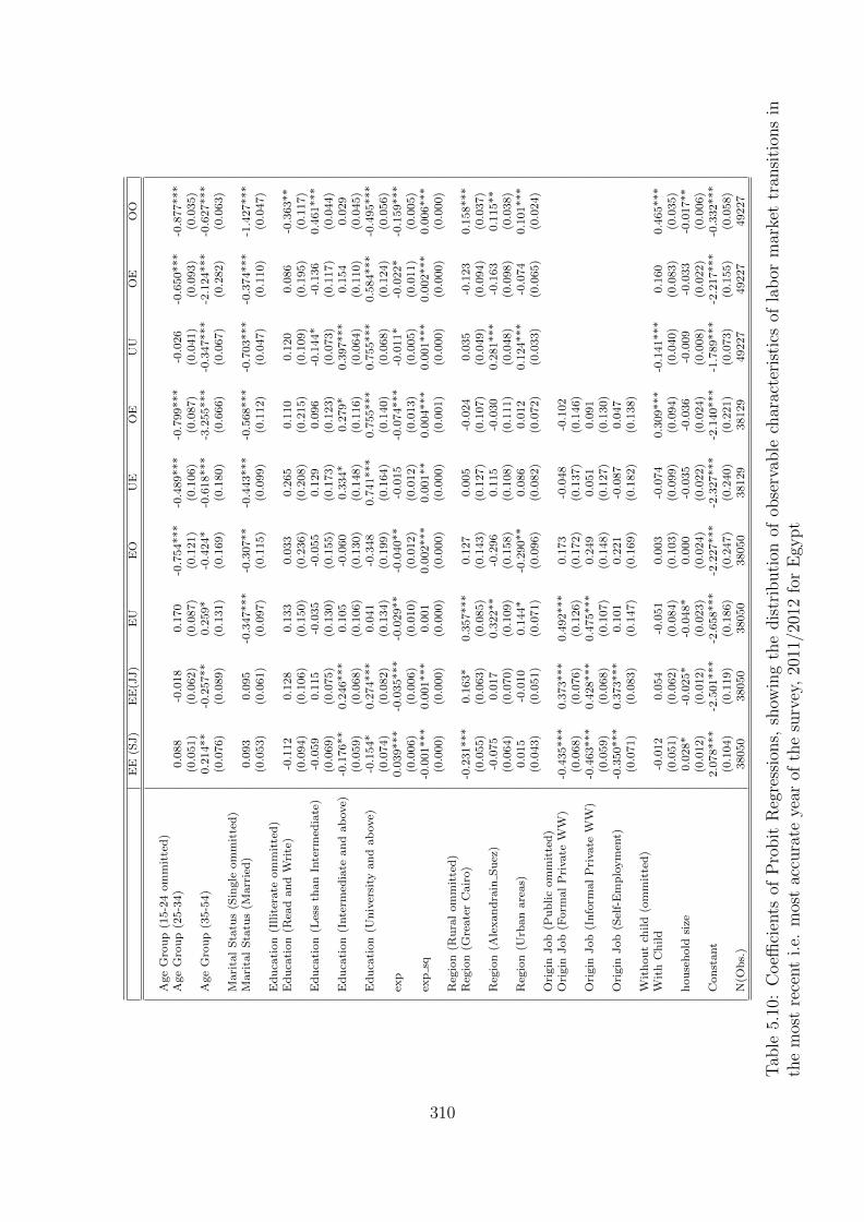
EE

(SJ)

EE

(JJ)

EU

EO

UE

OE

UU

OE

OO

Age

Gro

up

(15-2

4om

mit

ted)

Age

Gro

up

(25-3

4)

0.0

88

-0.0

18

0.1

70

-0.7

54***

-0.4

89***

-0.7

99***

-0.0

26

-0.6

50***

-0.8

77***

(0.0

51)

(0.0

62)

(0.0

87)

(0.1

21)

(0.1

06)

(0.0

87)

(0.0

41)

(0.0

93)

(0.0

35)

Age

Gro

up

(35-5

4)

0.2

14**

-0.2

57**

0.2

59*

-0.4

24*

-0.6

18***

-3.2

55***

-0.3

47***

-2.1

24***

-0.6

27***

(0.0

76)

(0.0

89)

(0.1

31)

(0.1

69)

(0.1

80)

(0.6

66)

(0.0

67)

(0.2

82)

(0.0

63)

Mari

tal

Sta

tus

(Sin

gle

om

mit

ted

)M

ari

tal

Sta

tus

(Marr

ied

)0.0

93

0.0

95

-0.3

47***

-0.3

07**

-0.4

43***

-0.5

68***

-0.7

03***

-0.3

74***

-1.4

27***

(0.0

53)

(0.0

61)

(0.0

97)

(0.1

15)

(0.0

99)

(0.1

12)

(0.0

47)

(0.1

10)

(0.0

47)

Ed

uca

tion

(Illit

erate

om

mit

ted

)E

du

cati

on

(Rea

dan

dW

rite

)-0

.112

0.1

28

0.1

33

0.0

33

0.2

65

0.1

10

0.1

20

0.0

86

-0.3

63**

(0.0

94)

(0.1

06)

(0.1

50)

(0.2

36)

(0.2

08)

(0.2

15)

(0.1

09)

(0.1

95)

(0.1

17)

Ed

uca

tion

(Les

sth

an

Inte

rmed

iate

)-0

.059

0.1

15

-0.0

35

-0.0

55

0.1

29

0.0

96

-0.1

44*

-0.1

36

0.4

61***

(0.0

69)

(0.0

75)

(0.1

30)

(0.1

55)

(0.1

73)

(0.1

23)

(0.0

73)

(0.1

17)

(0.0

44)

Ed

uca

tion

(Inte

rmed

iate

and

ab

ove)

-0.1

76**

0.2

46***

0.1

05

-0.0

60

0.3

34*

0.2

79*

0.3

97***

0.1

54

0.0

29

(0.0

59)

(0.0

68)

(0.1

06)

(0.1

30)

(0.1

48)

(0.1

16)

(0.0

64)

(0.1

10)

(0.0

45)

Ed

uca

tion

(Un

iver

sity

an

dab

ove)

-0.1

54*

0.2

74***

0.0

41

-0.3

48

0.7

41***

0.7

55***

0.7

55***

0.5

84***

-0.4

95***

(0.0

74)

(0.0

82)

(0.1

34)

(0.1

99)

(0.1

64)

(0.1

40)

(0.0

68)

(0.1

24)

(0.0

56)

exp

0.0

39***

-0.0

35***

-0.0

29**

-0.0

40**

-0.0

15

-0.0

74***

-0.0

11*

-0.0

22*

-0.1

59***

(0.0

06)

(0.0

06)

(0.0

10)

(0.0

12)

(0.0

12)

(0.0

13)

(0.0

05)

(0.0

11)

(0.0

05)

exp

sq-0

.001***

0.0

01***

0.0

01

0.0

02***

0.0

01**

0.0

04***

0.0

01***

0.0

02***

0.0

06***

(0.0

00)

(0.0

00)

(0.0

00)

(0.0

00)

(0.0

00)

(0.0

01)

(0.0

00)

(0.0

00)

(0.0

00)

Reg

ion

(Ru

ral

om

mit

ted)

Reg

ion

(Gre

ate

rC

air

o)

-0.2

31***

0.1

63*

0.3

57***

0.1

27

0.0

05

-0.0

24

0.0

35

-0.1

23

0.1

58***

(0.0

55)

(0.0

63)

(0.0

85)

(0.1

43)

(0.1

27)

(0.1

07)

(0.0

49)

(0.0

94)

(0.0

37)

Reg

ion

(Ale

xand

rain

Suez

)-0

.075

0.0

17

0.3

22**

-0.2

96

0.1

15

-0.0

30

0.2

81***

-0.1

63

0.1

15**

(0.0

64)

(0.0

70)

(0.1

09)

(0.1

58)

(0.1

08)

(0.1

11)

(0.0

48)

(0.0

98)

(0.0

38)

Reg

ion

(Urb

an

are

as)

0.0

15

-0.0

10

0.1

44*

-0.2

90**

0.0

86

0.0

12

0.1

24***

-0.0

74

0.1

01***

(0.0

43)

(0.0

51)

(0.0

71)

(0.0

96)

(0.0

82)

(0.0

72)

(0.0

33)

(0.0

65)

(0.0

24)

Ori

gin

Job

(Pub

lic

om

mit

ted)

Ori

gin

Job

(Form

al

Pri

vate

WW

)-0

.435***

0.3

73***

0.4

92***

0.1

73

-0.0

48

-0.1

02

(0.0

68)

(0.0

76)

(0.1

26)

(0.1

72)

(0.1

37)

(0.1

46)

Ori

gin

Job

(Info

rmal

Pri

vate

WW

)-0

.463***

0.4

28***

0.4

75***

0.2

49

0.0

51

0.0

91

(0.0

59)

(0.0

68)

(0.1

07)

(0.1

48)

(0.1

27)

(0.1

30)

Ori

gin

Job

(Sel

f-E

mplo

ym

ent)

-0.3

50***

0.3

73***

0.1

01

0.2

21

-0.0

87

0.0

47

(0.0

71)

(0.0

83)

(0.1

47)

(0.1

69)

(0.1

82)

(0.1

38)

Wit

hou

tch

ild

(om

mit

ted

)W

ith

Ch

ild

-0.0

12

0.0

54

-0.0

51

0.0

03

-0.0

74

0.3

09***

-0.1

41***

0.1

60

0.4

65***

(0.0

51)

(0.0

62)

(0.0

84)

(0.1

03)

(0.0

99)

(0.0

94)

(0.0

40)

(0.0

83)

(0.0

35)

hou

sehold

size

0.0

28*

-0.0

25*

-0.0

48*

0.0

00

-0.0

35

-0.0

36

-0.0

09

-0.0

33

-0.0

17**

(0.0

12)

(0.0

12)

(0.0

23)

(0.0

24)

(0.0

22)

(0.0

24)

(0.0

08)

(0.0

22)

(0.0

06)

Con

stant

2.0

78***

-2.5

01***

-2.6

58***

-2.2

27***

-2.3

27***

-2.1

40***

-1.7

89***

-2.2

17***

-0.3

32***

(0.1

04)

(0.1

19)

(0.1

86)

(0.2

47)

(0.2

40)

(0.2

21)

(0.0

73)

(0.1

55)

(0.0

58)

N(O

bs.

)38050

38050

38050

38050

38129

38129

49227

49227

49227

Tab

le5.

10:

Coeffi

cien

tsof

Pro

bit

Reg

ress

ions,

show

ing

the

dis

trib

uti

onof

obse

rvab

lech

arac

teri

stic

sof

lab

orm

arke

ttr

ansi

tion

sin

the

mos

tre

cent

i.e.

mos

tac

cura

teye

arof

the

surv

ey,

2011

/201

2fo

rE

gypt

310

EE

(SJ)

EE

(JJ)

EU

EO

UE

OE

UU

OU

OO

Age

Gro

up

(15-2

4om

mit

ted)

Age

Gro

up

(25-3

4)

0.0

26

-0.0

47

0.0

57

-0.2

22

-0.3

09***

-0.8

63***

-0.0

91

-0.3

75*

-0.8

17***

(0.0

62)

(0.0

73)

(0.0

90)

(0.1

67)

(0.0

78)

(0.1

35)

(0.0

50)

(0.1

63)

(0.0

40)

Age

Gro

up

(35-5

4)

0.0

32

-0.1

63

0.2

32*

0.4

12*

-0.7

59***

-0.7

72***

-0.4

18***

-0.1

99

-0.6

30***

(0.0

78)

(0.0

91)

(0.1

13)

(0.1

77)

(0.1

33)

(0.1

76)

(0.0

79)

(0.2

37)

(0.0

80)

Mari

tal

Sta

tus

(Sin

gle

om

mit

ted

)M

ari

tal

Sta

tus

(Marr

ied)

0.1

02

0.0

22

-0.3

07***

-0.5

24***

-0.3

62***

-0.6

16***

-0.6

54***

-0.1

19

-0.7

25***

(0.0

60)

(0.0

69)

(0.0

87)

(0.1

29)

(0.0

89)

(0.1

15)

(0.0

56)

(0.2

34)

(0.0

68)

Ed

uca

tion

(Illit

erate

om

mit

ted

)0.0

00

Ed

uca

tion

(Rea

dan

dW

rite

)0.0

00

-0.0

44

-0.0

49

0.4

04

-0.0

27

0.0

80

-0.0

44

-0.1

85

-0.1

60

(0.1

44)

(0.1

75)

(0.1

85)

(0.2

82)

(0.2

64)

(0.4

62)

(0.1

14)

(0.3

86)

(0.0

96)

Ed

uca

tion

(Les

sth

an

Inte

rmed

iate

)-0

.028

-0.0

50

0.1

16

0.2

73

0.2

57

0.1

05

0.3

87***

0.2

11

-0.7

65***

(0.1

34)

(0.1

62)

(0.1

64)

(0.2

76)

(0.2

18)

(0.4

07)

(0.1

04)

(0.3

58)

(0.0

86)

Ed

uca

tion

(Inte

rmed

iate

and

ab

ove)

-0.0

13

-0.0

34

0.0

10

0.3

74

0.1

61

0.3

75

0.0

80

0.0

58

-0.4

01***

(0.1

37)

(0.1

66)

(0.1

68)

(0.2

72)

(0.2

22)

(0.4

04)

(0.1

06)

(0.3

64)

(0.0

86)

Ed

uca

tion

(Un

iver

sity

an

dab

ove)

0.0

58

-0.0

42

-0.1

06

-0.5

57

0.3

57

0.6

34

0.5

43***

0.8

28*

-1.0

46***

(0.1

42)

(0.1

69)

(0.1

97)

(0.3

94)

(0.2

24)

(0.4

15)

(0.1

10)

(0.3

63)

(0.1

02)

exp

0.0

31***

-0.0

17

-0.0

50***

0.0

29

-0.0

55***

-0.1

58***

-0.0

05

-0.2

76***

-0.3

27***

(0.0

09)

(0.0

10)

(0.0

14)

(0.0

19)

(0.0

15)

(0.0

34)

(0.0

07)

(0.0

66)

(0.0

15)

exp

sq-0

.001***

0.0

01

0.0

02***

-0.0

00

0.0

04***

0.0

06***

0.0

02***

0.0

08***

0.0

12***

(0.0

00)

(0.0

00)

(0.0

00)

(0.0

01)

(0.0

00)

(0.0

01)

(0.0

00)

(0.0

02)

(0.0

01)

Reg

ion

(Ru

ral

Mid

dle

om

mit

ted)

0.0

00

Reg

ion

(Ru

ral

Nort

h)

-0.1

07

0.0

69

0.1

68

0.1

50

0.0

27

0.1

19

0.0

29

0.2

43

-0.0

31

(0.0

81)

(0.0

91)

(0.1

40)

(0.1

99)

(0.1

14)

(0.1

44)

(0.0

58)

(0.1

30)

(0.0

49)

Reg

ion

(Ru

ral

Sou

th)

0.1

06

-0.1

09

0.0

43

-0.3

27

-0.2

91*

-0.5

66*

0.2

27***

-0.0

05

-0.3

52***

(0.0

93)

(0.1

05)

(0.1

53)

(0.2

90)

(0.1

41)

(0.2

32)

(0.0

62)

(0.1

56)

(0.0

55)

Reg

ion

(Urb

an

Mid

dle

)0.0

42

-0.1

07

0.1

50

0.0

05

-0.1

63

-0.1

27

-0.1

25*

0.0

45

-0.1

39***

(0.0

64)

(0.0

73)

(0.1

08)

(0.1

59)

(0.0

96)

(0.1

16)

(0.0

49)

(0.1

15)

(0.0

39)

Reg

ion

(Urb

an

Nort

h)

-0.0

24

-0.0

34

0.1

78

0.0

04

-0.0

43

0.0

70

0.0

72

0.0

08

0.0

38

(0.0

68)

(0.0

77)

(0.1

13)

(0.1

77)

(0.0

96)

(0.1

24)

(0.0

50)

(0.1

20)

(0.0

42)

Reg

ion

(Urb

an

South

)0.0

14

-0.1

87

0.3

37*

0.0

34

-0.0

95

-0.2

73

0.2

72***

0.1

54

-0.2

83***

(0.0

90)

(0.1

07)

(0.1

43)

(0.2

10)

(0.1

35)

(0.1

70)

(0.0

59)

(0.1

44)

(0.0

58)

Ori

gin

/D

est.

Job

(Pub

lic

om

mit

ted)

0.0

00

Ori

gin

/D

est.

Job

(Form

al

Pri

vate

WW

)-0

.381***

0.5

05***

-0.0

19

-0.2

36

0.1

55

0.1

55

(0.0

58)

(0.0

67)

(0.1

11)

(0.2

04)

(0.0

92)

(0.1

14)

Ori

gin

/D

est.

Job

(Info

rmal

Pri

vate

WW

)-0

.461***

0.4

46***

0.3

70***

0.2

28*

0.1

65*

0.2

03

(0.0

54)

(0.0

65)

(0.0

82)

(0.1

15)

(0.0

84)

(0.1

09)

Ori

gin

/D

est.

Job

(Sel

f-E

mplo

ym

ent)

-0.3

15***

0.3

31***

0.2

55**

-0.0

20

-0.0

44

0.4

26***

(0.0

65)

(0.0

78)

(0.0

97)

(0.1

45)

(0.1

08)

(0.1

24)

Wit

hou

tch

ild

(om

mit

ted)

Wit

hC

hild

-0.0

01

-0.0

10

0.0

13

0.1

77

0.0

21

-0.3

55

0.1

85*

0.5

71

-0.1

28

(0.0

87)

(0.1

02)

(0.1

14)

(0.2

15)

(0.1

32)

(0.2

86)

(0.0

82)

(0.3

51)

(0.0

89)

hhsi

ze0.0

17

-0.0

24*

0.0

04

-0.0

04

0.0

14

0.0

18

0.0

12

0.0

18

0.0

11*

(0.0

10)

(0.0

12)

(0.0

12)

(0.0

22)

(0.0

13)

(0.0

15)

(0.0

06)

(0.0

15)

(0.0

05)

Con

stant

1.6

18***

-1.7

17***

-2.4

05***

-3.2

68***

-1.9

43***

-1.5

47**

-1.9

51***

-3.0

64***

1.1

80***

(0.1

86)

(0.2

24)

(0.2

34)

(0.3

65)

(0.2

72)

(0.4

73)

(0.1

41)

(0.4

88)

(0.1

20)

N(O

bs.

)16858

16858

16858

16858

17036

17036

25925

25925

25925

Tab

le5.

11:

Coeffi

cien

tsof

Pro

bit

Reg

ress

ions,

show

ing

the

dis

trib

uti

onof

obse

rvab

lech

arac

teri

stic

sof

lab

orm

arke

ttr

ansi

tion

sin

the

mos

tre

cent

i.e.

mos

tac

cura

teye

arof

the

surv

ey,

2009

/201

0fo

rJor

dan

311

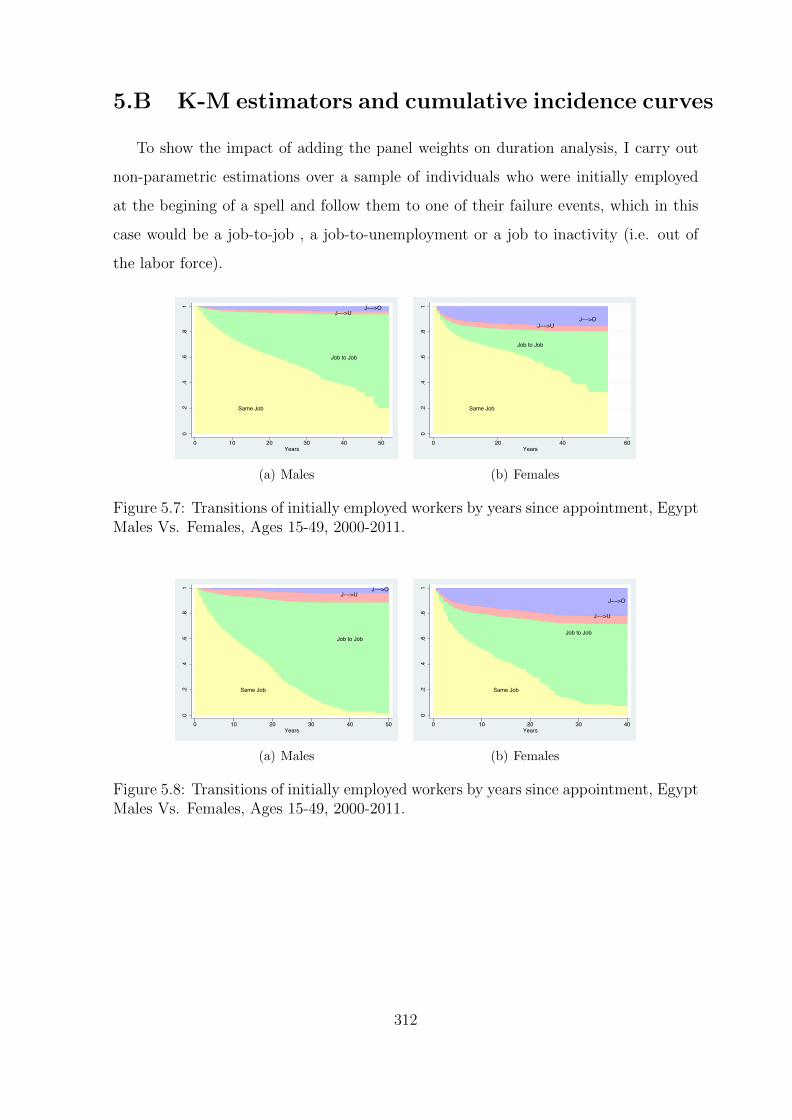
5.B K-M estimators and cumulative incidence curves

To show the impact of adding the panel weights on duration analysis, I carry out

non-parametric estimations over a sample of individuals who were initially employed

at the begining of a spell and follow them to one of their failure events, which in this

case would be a job-to-job , a job-to-unemployment or a job to inactivity (i.e. out of

the labor force).

Same Job

Job to Job

J−−>U J−−>O

0.2

.4.6

.81

0 10 20 30 40 50Years

(a) Males

Same Job

Job to Job

J−−>U J−−>O

0.2

.4.6

.81

0 20 40 60Years

(b) Females

Figure 5.7: Transitions of initially employed workers by years since appointment, EgyptMales Vs. Females, Ages 15-49, 2000-2011.

Same Job

Job to Job

J−−>U J−−>O

0.2

.4.6

.81

0 10 20 30 40 50Years

(a) Males

Same Job

Job to Job

J−−>U

J−−>O

0.2

.4.6

.81

0 10 20 30 40Years

(b) Females

Figure 5.8: Transitions of initially employed workers by years since appointment, EgyptMales Vs. Females, Ages 15-49, 2000-2011.

312

.2.4

.6.8

1

0 10 20 30 40 50Years since appointment

Raw Data Adding Proportional WeightsAdding Predicted Weights

(a) KM Survival Function

0.0

5.1

.15

.2.2

5

0 10 20 30 40 50Years since appointment

Raw Data Adding Proportional WeightsAdding Predicted Weights

(b) Job-to-job

0.0

1.0

2.0

3.0

4.0

5

0 10 20 30 40Years since appointment

Raw Data Adding Proportional WeightsAdding Predicted Weights

(c) Employment to Unemployment

0.0

2.0

4.0

6

0 10 20 30 40 50Years since appointment

Raw Data Adding Proportional WeightsAdding Predicted Weights

(d) Employment to Inactivity

Figure 5.9: The impact of adding proportional and predicted longitudinal panel weightsto the non-parametric Kaplan-Meier Survival and Cumulative Incidence Estimations,Male Workers, ages 15-49, Egypt.

313

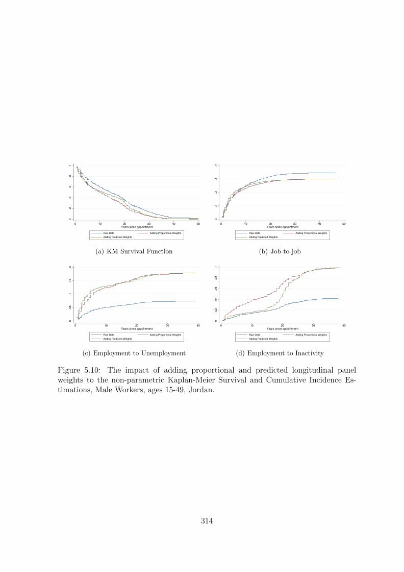
0.2

.4.6

.81

0 10 20 30 40 50Years since appointment

Raw Data Adding Proportional WeightsAdding Predicted Weights

(a) KM Survival Function

0.1

.2.3

.4

0 10 20 30 40 50Years since appointment

Raw Data Adding Proportional WeightsAdding Predicted Weights

(b) Job-to-job

0.0

5.1

.15

.2

0 10 20 30 40Years since appointment

Raw Data Adding Proportional WeightsAdding Predicted Weights

(c) Employment to Unemployment

0.0

2.0

4.0

6.0

8.1

0 10 20 30 40Years since appointment

Raw Data Adding Proportional WeightsAdding Predicted Weights

(d) Employment to Inactivity

Figure 5.10: The impact of adding proportional and predicted longitudinal panelweights to the non-parametric Kaplan-Meier Survival and Cumulative Incidence Es-timations, Male Workers, ages 15-49, Jordan.

314

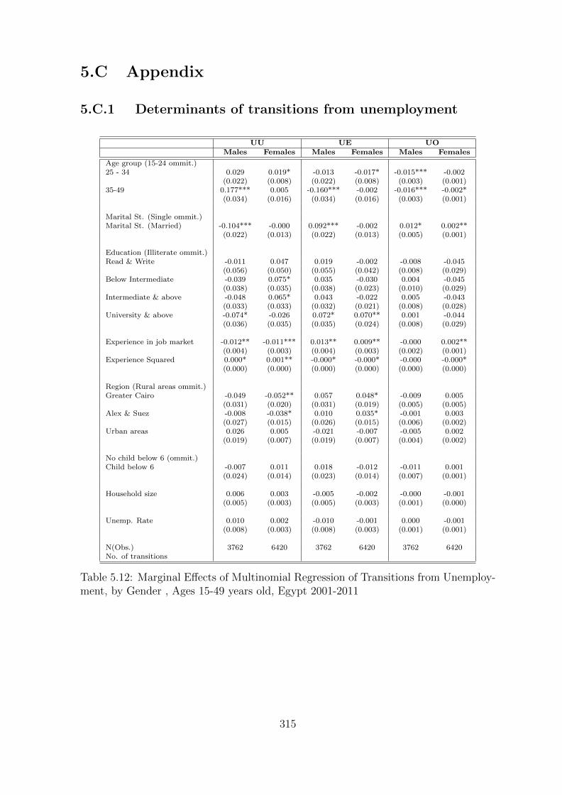
5.C Appendix

5.C.1 Determinants of transitions from unemployment

UU UE UOMales Females Males Females Males Females

Age group (15-24 ommit.)25 - 34 0.029 0.019* -0.013 -0.017* -0.015*** -0.002

(0.022) (0.008) (0.022) (0.008) (0.003) (0.001)35-49 0.177*** 0.005 -0.160*** -0.002 -0.016*** -0.002*

(0.034) (0.016) (0.034) (0.016) (0.003) (0.001)

Marital St. (Single ommit.)Marital St. (Married) -0.104*** -0.000 0.092*** -0.002 0.012* 0.002**

(0.022) (0.013) (0.022) (0.013) (0.005) (0.001)

Education (Illiterate ommit.)Read & Write -0.011 0.047 0.019 -0.002 -0.008 -0.045

(0.056) (0.050) (0.055) (0.042) (0.008) (0.029)Below Intermediate -0.039 0.075* 0.035 -0.030 0.004 -0.045

(0.038) (0.035) (0.038) (0.023) (0.010) (0.029)Intermediate & above -0.048 0.065* 0.043 -0.022 0.005 -0.043

(0.033) (0.033) (0.032) (0.021) (0.008) (0.028)University & above -0.074* -0.026 0.072* 0.070** 0.001 -0.044

(0.036) (0.035) (0.035) (0.024) (0.008) (0.029)

Experience in job market -0.012** -0.011*** 0.013** 0.009** -0.000 0.002**(0.004) (0.003) (0.004) (0.003) (0.002) (0.001)

Experience Squared 0.000* 0.001** -0.000* -0.000* -0.000 -0.000*(0.000) (0.000) (0.000) (0.000) (0.000) (0.000)

Region (Rural areas ommit.)Greater Cairo -0.049 -0.052** 0.057 0.048* -0.009 0.005

(0.031) (0.020) (0.031) (0.019) (0.005) (0.005)Alex & Suez -0.008 -0.038* 0.010 0.035* -0.001 0.003

(0.027) (0.015) (0.026) (0.015) (0.006) (0.002)Urban areas 0.026 0.005 -0.021 -0.007 -0.005 0.002

(0.019) (0.007) (0.019) (0.007) (0.004) (0.002)

No child below 6 (ommit.)Child below 6 -0.007 0.011 0.018 -0.012 -0.011 0.001

(0.024) (0.014) (0.023) (0.014) (0.007) (0.001)

Household size 0.006 0.003 -0.005 -0.002 -0.000 -0.001(0.005) (0.003) (0.005) (0.003) (0.001) (0.000)

Unemp. Rate 0.010 0.002 -0.010 -0.001 0.000 -0.001(0.008) (0.003) (0.008) (0.003) (0.001) (0.001)

N(Obs.) 3762 6420 3762 6420 3762 6420No. of transitions

Table 5.12: Marginal Effects of Multinomial Regression of Transitions from Unemploy-ment, by Gender , Ages 15-49 years old, Egypt 2001-2011

315

UU

UE

UO

raw

prop

orti

on

al

predic

ted

raw

prop

orti

on

al

predic

ted

raw

prop

orti

on

al

predic

ted

data

weig

hts

weig

hts

data

weig

hts

weig

hts

data

weig

hts

weig

hts

Age

gro

up

(15-2

4om

mit

.)25

-34

0.0

29

0.0

17

0.1

77***

-0.0

13

-0.0

06

-0.1

68***

-0.0

15***

-0.0

11***

-0.0

09***

(0.0

22)

(0.0

20)

(0.0

20)

(0.0

22)

(0.0

20)

(0.0

20)

(0.0

03)

(0.0

03)

(0.0

02)

35-4

90.1

77***

0.1

39***

0.2

51***

-0.1

60***

-0.1

27***

-0.2

41***

-0.0

16***

-0.0

12***

-0.0

10***

(0.0

34)

(0.0

31)

(0.0

20)

(0.0

34)

(0.0

31)

(0.0

20)

(0.0

03)

(0.0

03)

(0.0

02)

Mari

tal

St.

(Sin

gle

om

mit

.)M

ari

tal

St.

(Marr

ied

)-0

.104***

-0.0

61**

-0.1

41***

0.0

92***

0.0

55**

0.1

19***

0.0

12*

0.0

06

0.0

21**

(0.0

22)

(0.0

20)

(0.0

25)

(0.0

22)

(0.0

20)

(0.0

25)

(0.0

05)

(0.0

03)

(0.0

07)

Ed

uca

tion

(Illit

erate

om

mit

.)R

ead

&W

rite

-0.0

11

-0.0

10

-0.0

36

0.0

19

0.0

16

0.0

49

-0.0

08

-0.0

05

-0.0

13

(0.0

56)

(0.0

48)

(0.0

49)

(0.0

55)

(0.0

48)

(0.0

48)

(0.0

08)

(0.0

06)

(0.0

12)

Bel

ow

Inte

rmed

iate

-0.0

39

-0.0

36

-0.0

80*

0.0

35

0.0

32

0.0

63*

0.0

04

0.0

04

0.0

17

(0.0

38)

(0.0

33)

(0.0

34)

(0.0

38)

(0.0

32)

(0.0

31)

(0.0

10)

(0.0

08)

(0.0

19)

Inte

rmed

iate

&ab

ove

-0.0

48

-0.0

42

-0.0

74**

0.0

43

0.0

39

0.0

77**

0.0

05

0.0

03

-0.0

03

(0.0

33)

(0.0

28)

(0.0

27)

(0.0

32)

(0.0

27)

(0.0

25)

(0.0

08)

(0.0

06)

(0.0

12)

Un

iver

sity

&ab

ove

-0.0

74*

-0.0

73*

-0.1

29***

0.0

72*

0.0

71*

0.1

37***

0.0

01

0.0

02

-0.0

09

(0.0

36)

(0.0

31)

(0.0

33)

(0.0

35)

(0.0

31)

(0.0

31)

(0.0

08)

(0.0

06)

(0.0

13)

Exp

erie

nce

injo

bm

ark

et-0

.012**

-0.0

12**

-0.0

24***

0.0

13**

0.0

11**

0.0

23***

-0.0

00

0.0

01

0.0

01

(0.0

04)

(0.0

04)

(0.0

05)

(0.0

04)

(0.0

04)

(0.0

04)

(0.0

02)

(0.0

01)

(0.0

01)

Exp

erie

nce

Square

d0.0

00*

0.0

00*

0.0

01**

-0.0

00*

-0.0

00*

-0.0

01**

-0.0

00

-0.0

00

-0.0

00

(0.0

00)

(0.0

00)

(0.0

00)

(0.0

00)

(0.0

00)

(0.0

00)

(0.0

00)

(0.0

00)

(0.0

00)

Reg

ion

(Ru

ral

are

as

om

mit

.)G

reate

rC

air

o-0

.049

-0.0

45

-0.1

00**

0.0

57

0.0

49

0.1

05**

-0.0

09

-0.0

04

-0.0

05

(0.0

31)

(0.0

29)

(0.0

35)

(0.0

31)

(0.0

28)

(0.0

35)

(0.0

05)

(0.0

04)

(0.0

04)

Ale

x&

Su

ez-0

.008

-0.0

07

0.0

44

0.0

10

0.0

03

-0.0

42

-0.0

01

0.0

04

-0.0

01

(0.0

27)

(0.0

24)

(0.0

28)

(0.0

26)

(0.0

23)

(0.0

28)

(0.0

06)

(0.0

07)

(0.0

05)

Urb

an

are

as

0.0

26

0.0

19

0.0

28

-0.0

21

-0.0

16

-0.0

24

-0.0

05

-0.0

02

-0.0

04

(0.0

19)

(0.0

17)

(0.0

21)

(0.0

19)

(0.0

16)

(0.0

21)

(0.0

04)

(0.0

03)

(0.0

03)

No

child

bel

ow

6(o

mm

it.)

Child

bel

ow

6-0

.007

-0.0

15

-0.0

20

0.0

18

0.0

20

0.0

23

-0.0

11

-0.0

06

-0.0

02

(0.0

24)

(0.0

21)

(0.0

24)

(0.0

23)

(0.0

21)

(0.0

24)

(0.0

07)

(0.0

05)

(0.0

04)

Hou

seh

old

size

0.0

06

0.0

07

0.0

13

-0.0

05

-0.0

06

-0.0

12

-0.0

00

-0.0

01

-0.0

01

(0.0

05)

(0.0

05)

(0.0

07)

(0.0

05)

(0.0

05)

(0.0

07)

(0.0

01)

(0.0

01)

(0.0

01)

Un

emp

.R

ate

0.0

10

0.0

06

0.0

07

-0.0

10

-0.0

04

-0.0

06

0.0

00

-0.0

01

-0.0

01

(0.0

08)

(0.0

08)

(0.0

10)

(0.0

08)

(0.0

08)

(0.0

10)

(0.0

01)

(0.0

01)

(0.0

01)

N(O

bs.

)3762

3762

3762

3762

3762

3762

3762

3762

3762

No.

of

tran

siti

on

s

Tab

le5.

13:

Mar

ginal

Eff

ects

ofM

ult

inom

ial

Reg

ress

ion

ofT

ransi

tion

sfr

omU

nem

plo

ym

ent,

Mal

eW

orke

rs,

Age

s15

-49

year

sol

d,

Egy

pt

2001

-201

1

316

UU UE a

Males Females Males Females

15-2425 - 34 0.045 0.041 -0.045 -0.041

(0.033) (0.028) (0.033) (0.028)35-49 0.166*** -0.061 -0.166*** 0.061

(0.048) (0.050) (0.048) (0.050)

married=0married=1 -0.045 -0.015 0.045 0.015

(0.029) (0.030) (0.029) (0.030)

Ill.R&W -0.061 0.430 0.061 -0.430

(0.058) (0.322) (0.058) (0.322)Less than Int. -0.120* 0.365 0.120* -0.365

(0.052) (0.319) (0.052) (0.319)Int. & above -0.143** 0.441 0.143** -0.441

(0.054) (0.314) (0.054) (0.314)Univ & above -0.209*** 0.362 0.209*** -0.362

(0.059) (0.317) (0.059) (0.317)

exp -0.023*** -0.031* 0.023*** 0.031*(0.005) (0.012) (0.005) (0.012)

exp sq 0.001*** 0.002* -0.001*** -0.002*(0.000) (0.001) (0.000) (0.001)

middlenorth 0.043* 0.054 -0.043* -0.054

(0.020) (0.029) (0.020) (0.029)south 0.068** 0.118*** -0.068** -0.118***

(0.023) (0.029) (0.023) (0.029)

child=0child=1 -0.068 -0.006 0.068 0.006

(0.041) (0.046) (0.041) (0.046)

hhsize 0.006 -0.003 -0.006 0.003(0.004) (0.006) (0.004) (0.006)

UR official 0.022*** 0.008 -0.022*** -0.008(0.006) (0.008) (0.006) (0.008)

N(Obs.) 3544 1599 3544 1599No. of transitions

Table 5.14: Marginal Effects of Multinomial Regression of Transitions from Unemploy-ment, by Gender , Ages 15-49 years old, Jordan 2000-2010

aOnly 6 male transitions were observed for Jordan from Unemployment to inactivity. I thereforechose to drop this category from the analysis.

317

UU UEraw proportional predicted raw proportional predicteddata weights weights data weights weights

Age group (15-24 ommit.)25 - 34 0.045 0.044 0.130*** -0.045 -0.044 -0.130***

(0.033) (0.031) (0.030) (0.033) (0.031) (0.030)35-49 0.166*** 0.153*** 0.273*** -0.166*** -0.153*** -0.273***

(0.048) (0.045) (0.045) (0.048) (0.045) (0.045)

Marital St. (Single ommit.)Marital St. (Married) -0.045 -0.021 -0.045 0.045 0.021 0.045

(0.029) (0.027) (0.029) (0.029) (0.027) (0.029)

Education (Illiterate ommit.)Read & Write -0.061 -0.049 -0.100 0.061 0.049 0.100

(0.058) (0.053) (0.113) (0.058) (0.053) (0.113)Below Intermediate -0.120* -0.111* -0.058 0.120* 0.111* 0.058

(0.052) (0.048) (0.089) (0.052) (0.048) (0.089)Intermediate & above -0.143** -0.125* -0.112 0.143** 0.125* 0.112

(0.054) (0.050) (0.090) (0.054) (0.050) (0.090)University & above -0.209*** -0.193*** -0.141 0.209*** 0.193*** 0.141

(0.059) (0.055) (0.093) (0.059) (0.055) (0.093)

Experience in job market -0.023*** -0.023*** -0.013* 0.023*** 0.023*** 0.013*(0.005) (0.004) (0.005) (0.005) (0.004) (0.005)

Experience Squared 0.001*** 0.001*** 0.000 -0.001*** -0.001*** -0.000(0.000) (0.000) (0.000) (0.000) (0.000) (0.000)

Region (Middle ommit.)Region (North) 0.043* 0.041* 0.062* -0.043* -0.041* -0.062*

(0.020) (0.019) (0.024) (0.020) (0.019) (0.024)Region (South) 0.068** 0.068** 0.207*** -0.068** -0.068** -0.207***

(0.023) (0.021) (0.022) (0.023) (0.021) (0.022)

No child below 6 (ommit.)Child below 6 -0.068 -0.060 -0.014 0.068 0.060 0.014

(0.041) (0.038) (0.043) (0.041) (0.038) (0.043)

Household size 0.006 0.006 0.006 -0.006 -0.006 -0.006(0.004) (0.004) (0.004) (0.004) (0.004) (0.004)

Unemp. Rate 0.022*** 0.038*** 0.039*** -0.022*** -0.038*** -0.039***(0.006) (0.006) (0.006) (0.006) (0.006) (0.006)

N(Obs.) 3544 3544 3544 3544 3544 3544

Table 5.15: Marginal Effects of Multinomial Regression of Transitions from Unemploy-ment, Male Workers , Ages 15-49 years old, Jordan 2000-2010

318

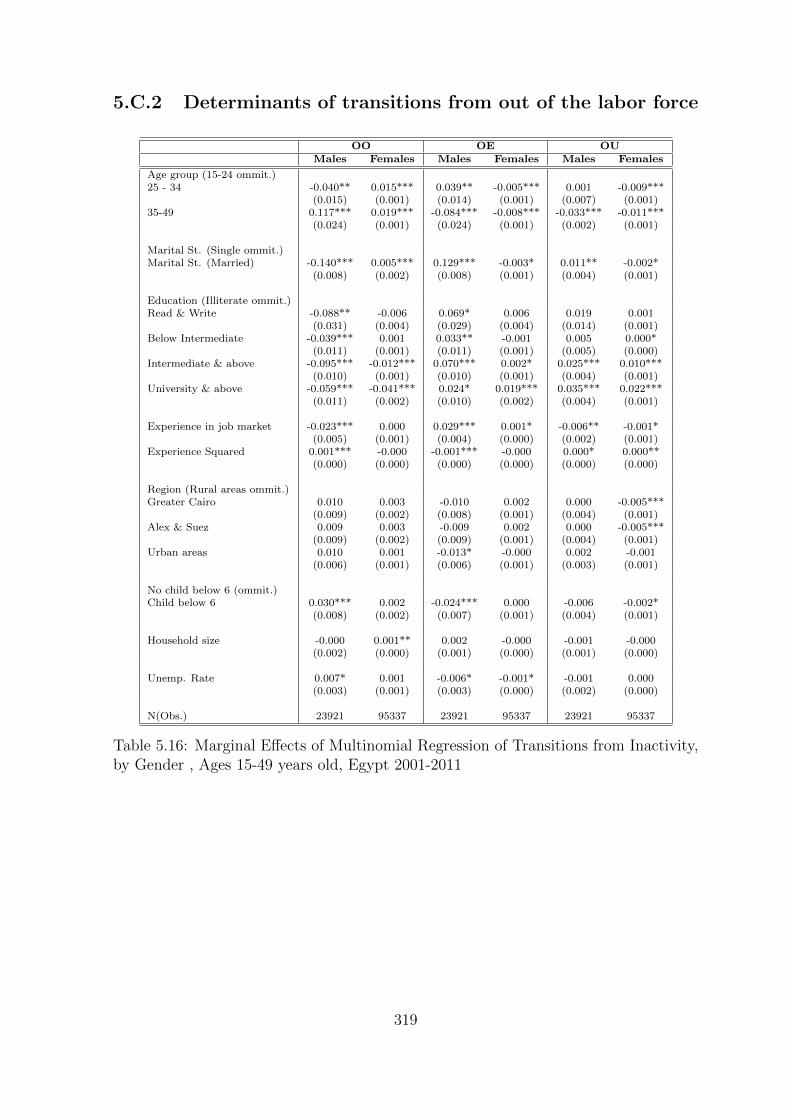
5.C.2 Determinants of transitions from out of the labor force

OO OE OUMales Females Males Females Males Females

Age group (15-24 ommit.)25 - 34 -0.040** 0.015*** 0.039** -0.005*** 0.001 -0.009***

(0.015) (0.001) (0.014) (0.001) (0.007) (0.001)35-49 0.117*** 0.019*** -0.084*** -0.008*** -0.033*** -0.011***

(0.024) (0.001) (0.024) (0.001) (0.002) (0.001)

Marital St. (Single ommit.)Marital St. (Married) -0.140*** 0.005*** 0.129*** -0.003* 0.011** -0.002*

(0.008) (0.002) (0.008) (0.001) (0.004) (0.001)

Education (Illiterate ommit.)Read & Write -0.088** -0.006 0.069* 0.006 0.019 0.001

(0.031) (0.004) (0.029) (0.004) (0.014) (0.001)Below Intermediate -0.039*** 0.001 0.033** -0.001 0.005 0.000*

(0.011) (0.001) (0.011) (0.001) (0.005) (0.000)Intermediate & above -0.095*** -0.012*** 0.070*** 0.002* 0.025*** 0.010***

(0.010) (0.001) (0.010) (0.001) (0.004) (0.001)University & above -0.059*** -0.041*** 0.024* 0.019*** 0.035*** 0.022***

(0.011) (0.002) (0.010) (0.002) (0.004) (0.001)

Experience in job market -0.023*** 0.000 0.029*** 0.001* -0.006** -0.001*(0.005) (0.001) (0.004) (0.000) (0.002) (0.001)

Experience Squared 0.001*** -0.000 -0.001*** -0.000 0.000* 0.000**(0.000) (0.000) (0.000) (0.000) (0.000) (0.000)

Region (Rural areas ommit.)Greater Cairo 0.010 0.003 -0.010 0.002 0.000 -0.005***

(0.009) (0.002) (0.008) (0.001) (0.004) (0.001)Alex & Suez 0.009 0.003 -0.009 0.002 0.000 -0.005***

(0.009) (0.002) (0.009) (0.001) (0.004) (0.001)Urban areas 0.010 0.001 -0.013* -0.000 0.002 -0.001

(0.006) (0.001) (0.006) (0.001) (0.003) (0.001)

No child below 6 (ommit.)Child below 6 0.030*** 0.002 -0.024*** 0.000 -0.006 -0.002*

(0.008) (0.002) (0.007) (0.001) (0.004) (0.001)

Household size -0.000 0.001** 0.002 -0.000 -0.001 -0.000(0.002) (0.000) (0.001) (0.000) (0.001) (0.000)

Unemp. Rate 0.007* 0.001 -0.006* -0.001* -0.001 0.000(0.003) (0.001) (0.003) (0.000) (0.002) (0.000)

N(Obs.) 23921 95337 23921 95337 23921 95337

Table 5.16: Marginal Effects of Multinomial Regression of Transitions from Inactivity,by Gender , Ages 15-49 years old, Egypt 2001-2011

319

OO

OE

OU

raw

prop

orti

on

al

predic

ted

raw

prop

orti

on

al

predic

ted

raw

prop

orti

on

al

predic

ted

data

weig

hts

weig

hts

data

weig

hts

weig

hts

data

weig

hts

weig

hts

Age

gro

up

(15-2

4om

mit

.)25

-34

-0.0

40**

-0.0

35**

-0.0

99***

0.0

39**

0.0

32**

0.0

19

0.0

01

0.0

03

0.0

79***

-0.0

15

(0.0

13)

(0.0

19)

-0.0

14

(0.0

12)

(0.0

13)

-0.0

07

(0.0

07)

(0.0

18)

35-4

90.1

17***

0.0

93***

0.1

19***

-0.0

84***

-0.0

61***

-0.0

89***

-0.0

33***

-0.0

32***

-0.0

31***

-0.0

24

(0.0

13)

(0.0

03)

-0.0

24

(0.0

13)

(0.0

03)

-0.0

02

(0.0

02)

(0.0

01)

Mari

tal

St.

(Sin

gle

om

mit

.)M

ari

tal

St.

(Marr

ied

)-0

.140***

-0.0

93***

-0.2

97***

0.1

29***

0.0

81***

0.1

93***

0.0

11**

0.0

12**

0.1

04***

-0.0

08

(0.0

07)

(0.0

12)

-0.0

08

(0.0

06)

(0.0

11)

-0.0

04

(0.0

04)

(0.0

11)

Ed

uca

tion

(Illit

erate

om

mit

.)R

ead

&W

rite

-0.0

88**

-0.0

67**

-0.1

39**

0.0

69*

0.0

47*

0.0

95*

0.0

19

0.0

20

0.0

43

-0.0

31

(0.0

26)

(0.0

47)

-0.0

29

(0.0

22)

(0.0

44)

-0.0

14

(0.0

15)

(0.0

27)

Bel

ow

Inte

rmed

iate

-0.0

39***

-0.0

28**

-0.0

08

0.0

33**

0.0

22**

0.0

04

0.0

05

0.0

05

0.0

04

-0.0

11

(0.0

09)

(0.0

07)

-0.0

11

(0.0

08)

(0.0

06)

-0.0

05

(0.0

04)

(0.0

04)

Inte

rmed

iate

&ab

ove

-0.0

95***

-0.0

73***

-0.0

69***

0.0

70***

0.0

48***

0.0

46***

0.0

25***

0.0

25***

0.0

23***

-0.0

1(0

.008)

(0.0

06)

-0.0

1(0

.007)

(0.0

06)

-0.0

04

(0.0

04)

(0.0

04)

Un

iver

sity

&ab

ove

-0.0

59***

-0.0

49***

-0.1

58***

0.0

24*

0.0

15*

0.1

16***

0.0

35***

0.0

35***

0.0

42***

-0.0

11

(0.0

08)

(0.0

09)

-0.0

1(0

.007)

(0.0

09)

-0.0

04

(0.0

04)

(0.0

05)

Exp

erie

nce

injo

bm

ark

et-0

.023***

-0.0

16***

-0.0

32***

0.0

29***

0.0

21***

0.0

31***

-0.0

06**

-0.0

05*

0.0

01

-0.0

05

(0.0

04)

(0.0

08)

-0.0

04

(0.0

03)

(0.0

09)

-0.0

02

(0.0

02)

(0.0

02)

Exp

erie

nce

Square

d0.0

01***

0.0

01**

0.0

01

-0.0

01***

-0.0

01***

-0.0

01

0.0

00*

0.0

00

-0.0

00

(0.0

00)

(0.0

00)

(0.0

01)

(0.0

00)

(0.0

00)

(0.0

01)

(0.0

00)

(0.0

00)

(0.0

00)

Reg

ion

(Ru

ral

are

as

om

mit

.)G

reate

rC

air

o0.0

10.0

11

0.0

35***

-0.0

1-0

.011

-0.0

30***

0.0

00

-0.0

00

-0.0

05

-0.0

09

(0.0

07)

(0.0

07)

-0.0

08

(0.0

06)

(0.0

06)

-0.0

04

(0.0

04)

(0.0

04)

Ale

x&

Su

ez0.0

09

0.0

07

0.0

23**

-0.0

09

-0.0

08

-0.0

20**

0.0

00

0.0

00

-0.0

03

-0.0

09

(0.0

08)

(0.0

08)

-0.0

09

(0.0

06)

(0.0

07)

-0.0

04

(0.0

04)

(0.0

04)

Urb

an

are

as

0.0

10.0

08

0.0

22***

-0.0

13*

-0.0

11*

-0.0

20***

0.0

02

0.0

02

-0.0

01

-0.0

06

(0.0

05)

(0.0

06)

-0.0

06

(0.0

04)

(0.0

05)

-0.0

03

(0.0

03)

(0.0

03)

No

child

bel

ow

6(o

mm

it.)

Child

bel

ow

60.0

30***

0.0

20**

0.0

31***

-0.0

24***

-0.0

13*

-0.0

10

-0.0

06

-0.0

06

-0.0

22***

-0.0

08

(0.0

06)

(0.0

07)

-0.0

07

(0.0

05)

(0.0

06)

-0.0

04

(0.0

04)

(0.0

04)

Hou

seh

old

size

-0.0

00

0.0

01

0.0

02

0.0

02

0.0

01

-0.0

02

-0.0

01

-0.0

01

-0.0

01

-0.0

02

(0.0

01)

(0.0

02)

-0.0

01

(0.0

01)

(0.0

01)

-0.0

01

(0.0

01)

(0.0

01)

Un

emp

.R

ate

0.0

07*

0.0

02

0.0

02

-0.0

06*

-0.0

01

-0.0

01

-0.0

01

-0.0

01

-0.0

01

-0.0

03

(0.0

03)

(0.0

03)

-0.0

03

(0.0

02)

(0.0

03)

-0.0

02

(0.0

02)

(0.0

02)

N(O

bs.

)23921

23921

23921

23921

23921

23921

23921

23921

23921

Tab

le5.

17:

Mar

ginal

Eff

ects

ofM

ult

inom

ial

Reg

ress

ion

ofT

ransi

tion

sfr

omIn

acti

vit

y,M

ale

Wor

kers

,A

ges

15-4

9ye

ars

old,

Egy

pt

2001

-201

1

320

OO OE OUMales Females Males Females Males Females

15-24 0.000 0.000 0.000 0.000 0.000 0.000(.) (.) (.) (.) (.) (.)

25 - 34 0.037* 0.008*** -0.048*** -0.008*** -0.048*** -0.000(0.016) (0.002) (0.010) (0.002) (0.010) (0.001)

35-49 0.084*** 0.017*** -0.058*** -0.011*** -0.058*** -0.006***(0.012) (0.002) (0.009) (0.002) (0.009) (0.001)

married=0 0.000 0.000 0.000 0.000 0.000 0.000(.) (.) (.) (.) (.) (.)

married=1 -0.086*** 0.009*** 0.070*** -0.002 0.070*** -0.008***(0.013) (0.002) (0.011) (0.001) (0.011) (0.001)

Ill. 0.000 0.000 0.000 0.000 0.000 0.000(.) (.) (.) (.) (.) (.)

R&W -0.027* -0.000 0.008 0.000 0.008 -0.000(0.011) (0.002) (0.008) (0.002) (0.008) (0.001)

Less than Int. -0.135*** -0.004 0.067*** 0.001 0.067*** 0.003***(0.009) (0.002) (0.008) (0.002) (0.008) (0.001)

Int. & above -0.067*** -0.012*** 0.043*** 0.005* 0.043*** 0.007***(0.008) (0.002) (0.007) (0.002) (0.007) (0.001)

Univ & above -0.101*** -0.061*** 0.051*** 0.028*** 0.051*** 0.033***(0.010) (0.004) (0.008) (0.003) (0.008) (0.003)

exp -0.018*** -0.003*** 0.023*** 0.004*** 0.023*** -0.001(0.004) (0.001) (0.004) (0.001) (0.004) (0.000)

exp sq 0.001*** 0.000** -0.001*** -0.000*** -0.001*** 0.000(0.000) (0.000) (0.000) (0.000) (0.000) (0.000)

middle 0.000 0.000 0.000 0.000 0.000 0.000(.) (.) (.) (.) (.) (.)

north 0.008 -0.002 -0.016*** -0.002* -0.016*** 0.004***(0.006) (0.002) (0.004) (0.001) (0.004) (0.001)

south -0.012 -0.010*** -0.013* -0.003* -0.013* 0.013***(0.008) (0.002) (0.005) (0.001) (0.005) (0.002)

child=0 0.000 0.000 0.000 0.000 0.000 0.000(.) (.) (.) (.) (.) (.)

child=1 -0.002 0.015** -0.006 -0.013** -0.006 -0.003(0.018) (0.005) (0.014) (0.004) (0.014) (0.003)

hhsize 0.001 0.000 -0.001 -0.000 -0.001 -0.000(0.001) (0.000) (0.001) (0.000) (0.001) (0.000)

UR official 0.004* 0.003*** -0.003* -0.000 -0.003* -0.003***(0.002) (0.000) (0.001) (0.000) (0.001) (0.000)

N(Obs.) 16280 52191 16280 52191 16280 52191No. Of transitions

Table 5.18: Marginal Effects of Multinomial Regression of Transitions from Inactivity,by Gender , Ages 15-49 years old, Jordan 2000-2010

321

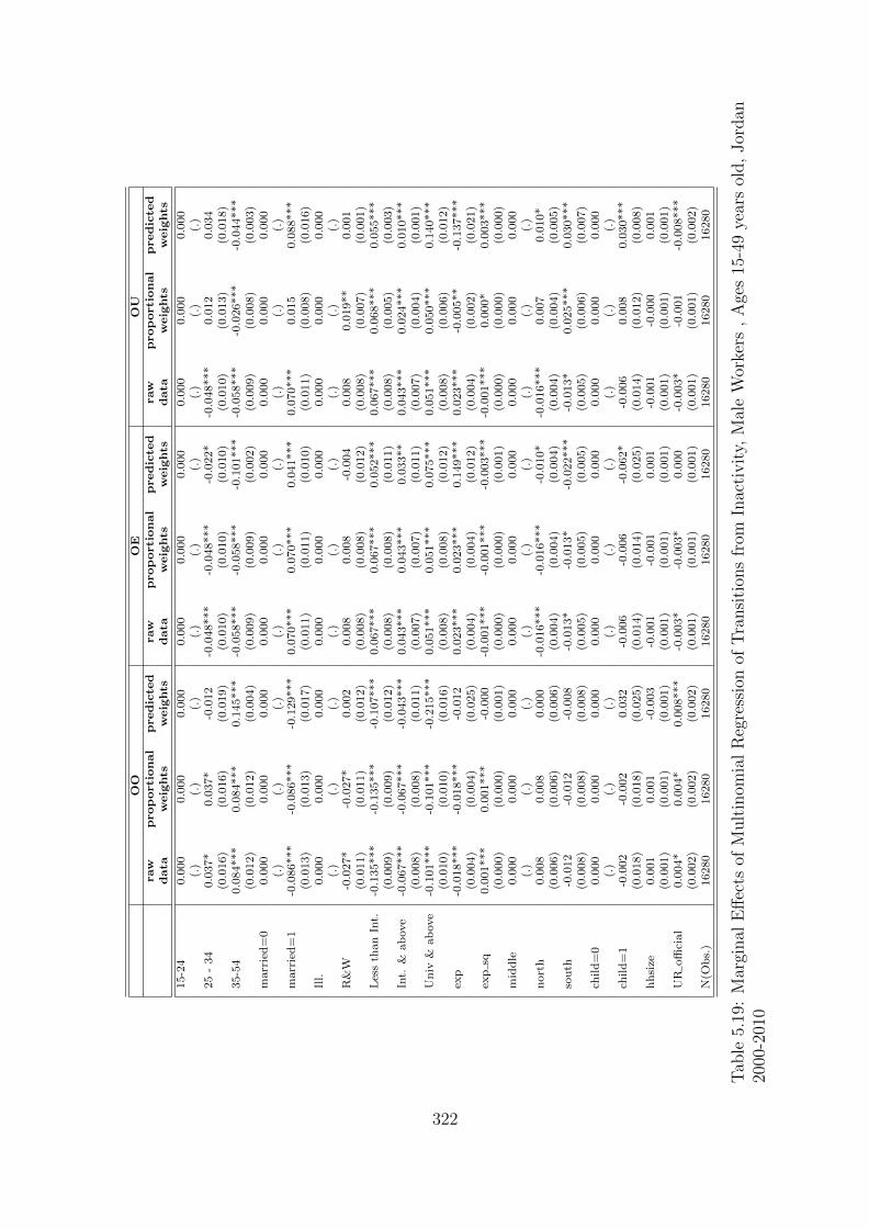
OO

OE

OU

raw

prop

orti

on

al

predic

ted

raw

prop

orti

on

al

predic

ted

raw

prop

orti

on

al

predic

ted

data

weig

hts

weig

hts

data

weig

hts

weig

hts

data

weig

hts

weig

hts

15-2

40.0

00

0.0

00

0.0

00

0.0

00

0.0

00

0.0

00

0.0

00

0.0

00

0.0

00

(.)

(.)

(.)

(.)

(.)

(.)

(.)

(.)

(.)

25

-34

0.0

37*

0.0

37*

-0.0

12

-0.0

48***

-0.0

48***

-0.0

22*

-0.0

48***

0.0

12

0.0

34

(0.0

16)

(0.0

16)

(0.0

19)

(0.0

10)

(0.0

10)

(0.0

10)

(0.0

10)

(0.0

13)

(0.0

18)

35-5

40.0

84***

0.0

84***

0.1

45***

-0.0

58***

-0.0

58***

-0.1

01***

-0.0

58***

-0.0

26***

-0.0

44***

(0.0

12)

(0.0

12)

(0.0

04)

(0.0

09)

(0.0

09)

(0.0

02)

(0.0

09)

(0.0

08)

(0.0

03)

marr

ied=

00.0

00

0.0

00

0.0

00

0.0

00

0.0

00

0.0

00

0.0

00

0.0

00

0.0

00

(.)

(.)

(.)

(.)

(.)

(.)

(.)

(.)

(.)

marr

ied=

1-0

.086***

-0.0

86***

-0.1

29***

0.0

70***

0.0

70***

0.0

41***

0.0

70***

0.0

15

0.0

88***

(0.0

13)

(0.0

13)

(0.0

17)

(0.0

11)

(0.0

11)

(0.0

10)

(0.0

11)

(0.0

08)

(0.0

16)

Ill.

0.0

00

0.0

00

0.0

00

0.0

00

0.0

00

0.0

00

0.0

00

0.0

00

0.0

00

(.)

(.)

(.)

(.)

(.)

(.)

(.)

(.)

(.)

R&

W-0

.027*

-0.0

27*

0.0

02

0.0

08

0.0

08

-0.0

04

0.0

08

0.0

19**

0.0

01

(0.0

11)

(0.0

11)

(0.0

12)

(0.0

08)

(0.0

08)

(0.0

12)

(0.0

08)

(0.0

07)

(0.0

01)

Les

sth

an

Int.

-0.1

35***

-0.1

35***

-0.1

07***

0.0

67***

0.0

67***

0.0

52***

0.0

67***

0.0

68***

0.0

55***

(0.0

09)

(0.0

09)

(0.0

12)

(0.0

08)

(0.0

08)

(0.0

11)

(0.0

08)

(0.0

05)

(0.0

03)

Int.

&ab

ove

-0.0

67***

-0.0

67***

-0.0

43***

0.0

43***

0.0

43***

0.0

33**

0.0

43***

0.0

24***

0.0

10***

(0.0

08)

(0.0

08)

(0.0

11)

(0.0

07)

(0.0

07)

(0.0

11)

(0.0

07)

(0.0

04)

(0.0

01)

Un

iv&

ab

ove

-0.1

01***

-0.1

01***

-0.2

15***

0.0

51***

0.0

51***

0.0

75***

0.0

51***

0.0

50***

0.1

40***

(0.0

10)

(0.0

10)

(0.0

16)

(0.0

08)

(0.0

08)

(0.0

12)

(0.0

08)

(0.0

06)

(0.0

12)

exp

-0.0

18***

-0.0

18***

-0.0

12

0.0

23***

0.0

23***

0.1

49***

0.0

23***

-0.0

05**

-0.1

37***

(0.0

04)

(0.0

04)

(0.0

25)

(0.0

04)

(0.0

04)

(0.0

12)

(0.0

04)

(0.0

02)

(0.0

21)

exp

sq0.0

01***

0.0

01***

-0.0

00

-0.0

01***

-0.0

01***

-0.0

03***

-0.0

01***

0.0

00*

0.0

03***

(0.0

00)

(0.0

00)

(0.0

01)

(0.0

00)

(0.0

00)

(0.0

01)

(0.0

00)

(0.0

00)

(0.0

00)

mid

dle

0.0

00

0.0

00

0.0

00

0.0

00

0.0

00

0.0

00

0.0

00

0.0

00

0.0

00

(.)

(.)

(.)

(.)

(.)

(.)

(.)

(.)

(.)

nort

h0.0

08

0.0

08

0.0

00

-0.0

16***

-0.0

16***

-0.0

10*

-0.0

16***

0.0

07

0.0

10*

(0.0

06)

(0.0

06)

(0.0

06)

(0.0

04)

(0.0

04)

(0.0

04)

(0.0

04)

(0.0

04)

(0.0

05)

south

-0.0

12

-0.0

12

-0.0

08

-0.0

13*

-0.0

13*

-0.0

22***

-0.0

13*

0.0

25***

0.0

30***

(0.0

08)

(0.0

08)

(0.0

08)

(0.0

05)

(0.0

05)

(0.0

05)

(0.0

05)

(0.0

06)

(0.0

07)

child

=0

0.0

00

0.0

00

0.0

00

0.0

00

0.0

00

0.0

00

0.0

00

0.0

00

0.0

00

(.)

(.)

(.)

(.)

(.)

(.)

(.)

(.)

(.)

child

=1

-0.0

02

-0.0

02

0.0

32

-0.0

06

-0.0

06

-0.0

62*

-0.0

06

0.0

08

0.0

30***

(0.0

18)

(0.0

18)

(0.0

25)

(0.0

14)

(0.0

14)

(0.0

25)

(0.0

14)

(0.0

12)

(0.0

08)

hhsi

ze0.0

01

0.0

01

-0.0

03

-0.0

01

-0.0

01

0.0

01

-0.0

01

-0.0

00

0.0

01

(0.0

01)

(0.0

01)

(0.0

01)

(0.0

01)

(0.0

01)

(0.0

01)

(0.0

01)

(0.0

01)

(0.0

01)

UR

offi

cial

0.0

04*

0.0

04*

0.0

08***

-0.0

03*

-0.0

03*

0.0

00

-0.0

03*

-0.0

01

-0.0

08***

(0.0

02)

(0.0

02)

(0.0

02)

(0.0

01)

(0.0

01)

(0.0

01)

(0.0

01)

(0.0

01)

(0.0

02)

N(O

bs.

)16280

16280

16280

16280

16280

16280

16280

16280

16280

Tab

le5.

19:

Mar

ginal

Eff

ects

ofM

ult

inom

ial

Reg

ress

ion

ofT

ransi

tion

sfr

omIn

acti

vit

y,M

ale

Wor

kers

,A

ges

15-4

9ye

ars

old,

Jor

dan

2000

-201

0

322

5.C.3 Detailed Transitions

323

NE–>NE

NE

–>

GNE

–>

FFemales

Males

Males

Males

Females

Males

Males

Males

Females

Males

Males

Males

No

weights

Pro

p.W

eights

Pre

d.W

eights

No

weights

Pro

p.W

eights

Pre

d.W

eights

No

weights

Pro

p.W

eights

Pre

d.W

eights

Agegro

up

(15-2

4ommit.)

25

-34

0.004**

-0.027**

-0.031***

0.065***

-0.001

0.031***

0.027***

-0.002

-0.001

0.012**

0.011**

-0.008***

(0.001)

(0.010)

(0.009)

(0.006)

(0.001)

(0.005)

(0.004)

(0.003)

(0.001)

(0.005)

(0.004)

(0.002)

35-5

40.008***

0.092***

0.061***

0.107***

-0.002*

-0.002

0.001

-0.014***

-0.001*

-0.009

-0.007*

-0.014***

(0.001)

(0.015)

(0.011)

(0.005)

(0.001)

(0.006)

(0.005)

(0.002)

(0.001)

(0.005)

(0.003)

(0.001)

Marita

lSt.

(Sin

gle

ommit.)

Marita

lSt.

(Married)

0.004**

-0.128***

-0.082***

-0.183***

0.001

0.024***

0.016***

0.035***

-0.001*

0.026***

0.018***

0.031***

(0.001)

(0.007)

(0.006)

(0.010)

(0.001)

(0.003)

(0.002)

(0.005)

(0.001)

(0.003)

(0.002)

(0.005)

Education

(Illitera

teommit.)

Read

&W

rite

-0.007*

-0.067**

-0.048*

-0.086*

0.004*

0.002

0.002

0.002

0.000

0.008

0.006

0.008

(0.004)

(0.025)

(0.020)

(0.034)

(0.002)

(0.004)

(0.003)

(0.003)

(0.000)

(0.005)

(0.004)

(0.005)

Below

Inte

rmediate

-0.000

-0.027*

-0.019*

-0.002

0.000

0.004

0.003

0.000

0.000

0.007**

0.005**

0.001

(0.001)

(0.011)

(0.008)

(0.006)

(0.000)

(0.002)

(0.002)

(0.001)

(0.000)

(0.003)

(0.002)

(0.001)

Inte

rmediate

&above

-0.006***

-0.061***

-0.044***

-0.049***

0.004***

0.011***

0.008***

0.005***

0.002***

0.015***

0.011***

0.006***

(0.001)

(0.009)

(0.007)

(0.006)

(0.000)

(0.002)

(0.001)

(0.001)

(0.000)

(0.002)

(0.001)

(0.001)

University

&above

-0.031***

-0.022*

-0.017*

-0.123***

0.028***

0.026***

0.019***

0.035***

0.004***

0.027***

0.019***

0.032***

(0.002)

(0.010)

(0.008)

(0.009)

(0.002)

(0.003)

(0.002)

(0.005)

(0.001)

(0.003)

(0.002)

(0.003)

Experiencein

job

mark

et

-0.003***

-0.025***

-0.019***

-0.031***

0.001**

0.001

0.001

0.002**

0.001***

0.006***

0.005***

0.008***

(0.001)

(0.003)

(0.002)

(0.005)

(0.000)

(0.001)

(0.001)

(0.001)

(0.000)

(0.001)

(0.001)

(0.002)

ExperienceSquare

d0.000***

0.001***

0.001***

0.001**

-0.000

-0.000

-0.000

-0.000

-0.000**

-0.000***

-0.000***

-0.001*

(0.000)

(0.000)

(0.000)

(0.000)

(0.000)

(0.000)

(0.000)

(0.000)

(0.000)

(0.000)

(0.000)

(0.000)

Region

(Rura

lare

asommit.)

Gre

ate

rCairo

-0.001

0.004

0.005

0.019**

-0.002*

0.000

-0.001

-0.007**

0.003***

0.014***

0.009***

0.010***

(0.002)

(0.008)

(0.006)

(0.007)

(0.001)

(0.003)

(0.002)

(0.002)

(0.001)

(0.003)

(0.002)

(0.003)

Alex

&Suez

-0.001

0.007

0.006

0.024**

0.000

0.011**

0.006*

0.007

0.002**

0.012**

0.008**

0.004

(0.001)

(0.008)

(0.006)

(0.008)

(0.001)

(0.004)

(0.003)

(0.004)

(0.001)

(0.004)

(0.003)

(0.004)

Urb

an

are

as

0.001

0.011*

0.009*

0.018**

0.001

-0.001

-0.001

-0.002

-0.000

-0.003

-0.002

-0.001

(0.001)

(0.006)

(0.004)

(0.005)

(0.001)

(0.002)

(0.002)

(0.003)

(0.000)

(0.002)

(0.001)

(0.002)

No

child

below

6(o

mmit.)

Child

below

60.001

0.025***

0.014**

0.018**

0.000

-0.001

-0.001

-0.003

-0.002*

-0.005

-0.004*

-0.007*

(0.001)

(0.007)

(0.005)

(0.007)

(0.001)

(0.002)

(0.002)

(0.003)

(0.001)

(0.003)

(0.002)

(0.003)

House

hold

size

0.001**

-0.000

0.000

0.003

-0.000

0.001

0.000

0.001

0.000

-0.001*

-0.001

-0.001

(0.000)

(0.001)

(0.001)

(0.002)

(0.000)

(0.000)

(0.000)

(0.001)

(0.000)

(0.001)

(0.001)

(0.001)

Unemp.Rate

0.001*

0.008**

0.003

0.003

-0.000

-0.002

-0.001

-0.002

0.000

-0.003*

-0.002

-0.004

(0.000)

(0.003)

(0.002)

(0.003)

(0.000)

(0.001)

(0.001)

(0.002)

(0.000)

(0.001)

(0.001)

(0.002)

N(O

bs.)

101757

27683

27683

27683

101757

27683

27683

27683

101757

27683

27683

27683

Tab

le5.

20:

Egy

pt

324

NE

–>

IN

E–>

NW

Fem

ale

sM

ale

sM

ale

sM

ale

sF

emale

sM

ale

sM

ale

sM

ale

sN

ow

eights

Pro

p.

Wei

ghts

Pre

d.

Wei

ghts

No

wei

ghts

Pro

p.

Wei

ghts

Pre

d.

Wei

ghts

Age

gro

up

(15-2

4om

mit

.)25

-34

-0.0

02**

-0.0

12

-0.0

04

-0.0

40***

0.0

00

-0.0

04

-0.0

02

-0.0

15***

(0.0

01)

(0.0

08)

(0.0

06)

(0.0

04)

(0.0

01)

(0.0

04)

(0.0

03)

(0.0

02)

35-5

4-0

.004***

-0.0

71***

-0.0

48***

-0.0

61***

-0.0

00

-0.0

08

-0.0

07

-0.0

19***

(0.0

01)

(0.0

08)

(0.0

06)

(0.0

04)

(0.0

01)

(0.0

10)

(0.0

06)

(0.0

02)

Mari

tal

St.

(Sin

gle

om

mit

.)M

ari

tal

St.

(Marr

ied

)-0

.003**

0.0

58***

0.0

36***

0.0

90***

-0.0

01

0.0

20***

0.0

12***

0.0

28***

(0.0

01)

(0.0

06)

(0.0

04)

(0.0

08)

(0.0

01)

(0.0

03)

(0.0

02)

(0.0

04)

Ed

uca

tion

(Illit

erate

om

mit

.)R

ead

&W

rite

0.0

01

0.0

44

0.0

30

0.0

67*

0.0

01

0.0

13

0.0

10

0.0

09

(0.0

02)

(0.0

23)

(0.0

18)

(0.0

33)

(0.0

02)

(0.0

08)

(0.0

06)

(0.0

05)

Bel

ow

Inte

rmed

iate

0.0

01

0.0

03

0.0

01

-0.0

03

-0.0

01

0.0

12**

0.0

10**

0.0

05**

(0.0

01)

(0.0

09)

(0.0

07)

(0.0

05)

(0.0

01)

(0.0

04)

(0.0

03)

(0.0

02)

Inte

rmed

iate

&ab

ove

0.0

01

0.0

18*

0.0

13

0.0

27***

-0.0

01

0.0

16***

0.0

12***

0.0

12***

(0.0

01)

(0.0

09)

(0.0

07)

(0.0

05)

(0.0

01)

(0.0

03)

(0.0

02)

(0.0

01)

Un

iver

sity

&ab

ove

0.0

01

-0.0

38***

-0.0

27***

0.0

32***

-0.0

02***

0.0

07*

0.0

05*

0.0

24***

(0.0

01)

(0.0

09)

(0.0

06)

(0.0

07)

(0.0

01)

(0.0

03)

(0.0

02)

(0.0

03)

Exp

erie

nce

injo

bm

ark

et0.0

01**

0.0

13***

0.0

10***

0.0

16***

0.0

00

0.0

04***

0.0

03***

0.0

04***

(0.0

00)

(0.0

02)

(0.0

02)

(0.0

04)

(0.0

00)

(0.0

01)

(0.0

01)

(0.0

01)

Exp

erie

nce

Square

d-0

.000

-0.0

01**

-0.0

00***

-0.0

01

-0.0

00

-0.0

00***

-0.0

00***

-0.0

00**

(0.0

00)

(0.0

00)

(0.0

00)

(0.0

00)

(0.0

00)

(0.0

00)

(0.0

00)

(0.0

00)

Reg

ion

(Ru

ral

are

as

om

mit

.)G

reate

rC

air

o0.0

03***

0.0

02

0.0

02

-0.0

03

-0.0

03***

-0.0

20***

-0.0

15***

-0.0

20***

(0.0

01)

(0.0

07)

(0.0

05)

(0.0

06)

(0.0

01)

(0.0

03)

(0.0

02)

(0.0

02)

Ale

x&

Su

ez0.0

03**

-0.0

09

-0.0

05

-0.0

16**

-0.0

03***

-0.0

21***

-0.0

15***

-0.0

19***

(0.0

01)

(0.0

06)

(0.0

05)

(0.0

06)

(0.0

00)

(0.0

03)

(0.0

02)

(0.0

02)

Urb

an

are

as

0.0

01

-0.0

06

-0.0

04

-0.0

12**

-0.0

02***

-0.0

01

-0.0

01

-0.0

03

(0.0

00)

(0.0

04)

(0.0

03)

(0.0

04)

(0.0

00)

(0.0

03)

(0.0

02)

(0.0

03)

No

child

bel

ow

6(o

mm

it.)

Child

bel

ow

6-0

.000

-0.0

10

-0.0

04

-0.0

03

0.0

01

-0.0

09*

-0.0

06*

-0.0

04

(0.0

01)

(0.0

05)

(0.0

04)

(0.0

05)

(0.0

01)

(0.0

04)

(0.0

03)

(0.0

03)

Hou

seh

old

size

-0.0

01***

-0.0

01

-0.0

01

-0.0

03**

0.0

00

0.0

02***

0.0

01***

0.0

01

(0.0

00)

(0.0

01)

(0.0

01)

(0.0

01)

(0.0

00)

(0.0

01)

(0.0

00)

(0.0

01)

Un

emp

.R

ate

-0.0

00

-0.0

02

0.0

01

0.0

03

-0.0

00*

-0.0

01

-0.0

00

0.0

00

(0.0

00)

(0.0

02)

(0.0

02)

(0.0

02)

(0.0

00)

(0.0

01)

(0.0

01)

(0.0

01)

N(O

bs.

)101757

27683

27683

27683

101757

27683

27683

27683

No.

of

tran

siti

on

s

Tab

le5.

21:

Egy

pt

325

NE–>NE

NE

–>

GNE

–>

FFemales

Males

Males

Males

Females

Males

Males

Males

Females

Males

Males

Males

No

weights

Pro

p.W

eights

Pre

d.W

eights

No

weights

Pro

p.W

eights

Pre

d.W

eights

No

weights

Pro

p.W

eights

Pre

d.W

eights

Agegro

up

(15-2

4ommit.)

25

-34

0.007**

0.017

0.017

0.053***

0.001

-0.004

-0.004

-0.015**

-0.005***

0.002

0.002

-0.003

(0.002)

(0.013)

(0.013)

(0.014)

(0.001)

(0.005)

(0.005)

(0.005)

(0.001)

(0.007)

(0.007)

(0.008)

35-5

40.012***

0.069***

0.069***

0.115***

-0.002*

-0.022***

-0.022***

-0.029***

-0.006***

-0.015***

-0.015***

-0.023***

(0.002)

(0.011)

(0.011)

(0.015)

(0.001)

(0.004)

(0.004)

(0.006)

(0.001)

(0.005)

(0.005)

(0.005)

Marita

lSt.

(Sin

gle

ommit.)

Marita

lSt.

(Married)

0.006***

-0.068***

-0.068***

-0.050***

0.001

0.045***

0.045***

0.026***

-0.004***

0.012*

0.012*

0.015*

(0.002)

(0.010)

(0.010)

(0.011)

(0.001)

(0.007)

(0.007)

(0.007)

(0.001)

(0.005)

(0.005)

(0.006)

Education

(Illitera

teommit.)

Read

&W

rite

-0.001

-0.021*

-0.021*

0.003

0.000

0.003

0.003

-0.003

0.001

0.002

0.002

-0.008

(0.002)

(0.010)

(0.010)

(0.015)

(0.001)

(0.004)

(0.004)

(0.004)

(0.001)

(0.004)

(0.004)

(0.008)

Below

Inte

rmediate

-0.004*

-0.093***

-0.093***

-0.084***

0.001*

0.028***

0.028***

0.027***

0.001

0.015***

0.015***

0.007

(0.002)

(0.008)

(0.008)

(0.014)

(0.001)

(0.003)

(0.003)

(0.005)

(0.001)

(0.003)

(0.003)

(0.008)

Inte

rmediate

&above

-0.009***

-0.057***

-0.057***

-0.034*

0.003***

0.022***

0.022***

0.014**

0.004***

0.014***

0.014***

0.004

(0.002)

(0.008)

(0.008)

(0.013)

(0.001)

(0.003)

(0.003)

(0.005)

(0.001)

(0.003)

(0.003)

(0.008)

University

&above

-0.045***

-0.083***

-0.083***

-0.120***

0.023***

0.034***

0.034***

0.047***

0.018***

0.041***

0.041***

0.053***

(0.004)

(0.009)

(0.009)

(0.015)

(0.002)

(0.004)

(0.004)

(0.006)

(0.002)

(0.005)

(0.005)

(0.010)

Experiencein

job

mark

et

-0.007***

-0.024***

-0.024***

-0.031***

0.002***

0.007***

0.007***

0.009***

0.003**

0.005***

0.005***

0.009***

(0.001)

(0.002)

(0.002)

(0.003)

(0.000)

(0.001)

(0.001)

(0.002)

(0.001)

(0.001)

(0.001)

(0.001)

ExperienceSquare

d0.000***

0.001***

0.001***

0.001***

-0.000*

-0.000***

-0.000***

-0.000**

-0.000

-0.000***

-0.000***

-0.000***

(0.000)

(0.000)

(0.000)

(0.000)

(0.000)

(0.000)

(0.000)

(0.000)

(0.000)

(0.000)

(0.000)

(0.000)

Region

(Mid

dle

ommit.)

Region

(North)

0.001

0.018***

0.018***

0.010

0.002**

0.022***

0.022***

0.026***

-0.003**

-0.016***

-0.016***

-0.018***

(0.001)

(0.005)

(0.005)

(0.006)

(0.001)

(0.003)

(0.003)

(0.003)

(0.001)

(0.002)

(0.002)

(0.003)

Region

(South

)-0

.000

0.011

0.011

0.039***

0.007***

0.042***

0.042***

0.026***

-0.003**

-0.017***

-0.017***

-0.023***

(0.002)

(0.006)

(0.006)

(0.006)

(0.001)

(0.004)

(0.004)

(0.004)

(0.001)

(0.003)

(0.003)

(0.003)

No

child

below

6(o

mmit.)

Child

below

60.017***

-0.009

-0.009

0.069**

-0.004

-0.002

-0.002

-0.030*

-0.009**

0.007

0.007

-0.015

(0.005)

(0.013)

(0.013)

(0.022)

(0.002)

(0.006)

(0.006)

(0.012)

(0.003)

(0.005)

(0.005)

(0.013)

House

hold

size

0.000

0.003*

0.003*

0.000

0.000

0.001*

0.001*

0.002**

-0.000

0.000

0.000

0.001

(0.000)

(0.001)

(0.001)

(0.001)

(0.000)

(0.000)

(0.000)

(0.001)

(0.000)

(0.000)

(0.000)

(0.001)

Unemp.Rate

0.001*

0.011***

0.011***

0.011***

-0.000

-0.005***

-0.005***

-0.005***

-0.001*

-0.004***

-0.004***

-0.005***

(0.000)

(0.002)

(0.002)

(0.002)

(0.000)

(0.001)

(0.001)

(0.001)

(0.000)

(0.001)

(0.001)

(0.001)

N(O

bs.)

53790

19824

19824

19824

53790

19824

19824

19824

53790

19824

19824

19824

Tab

le5.

22:

Jor

dan

326

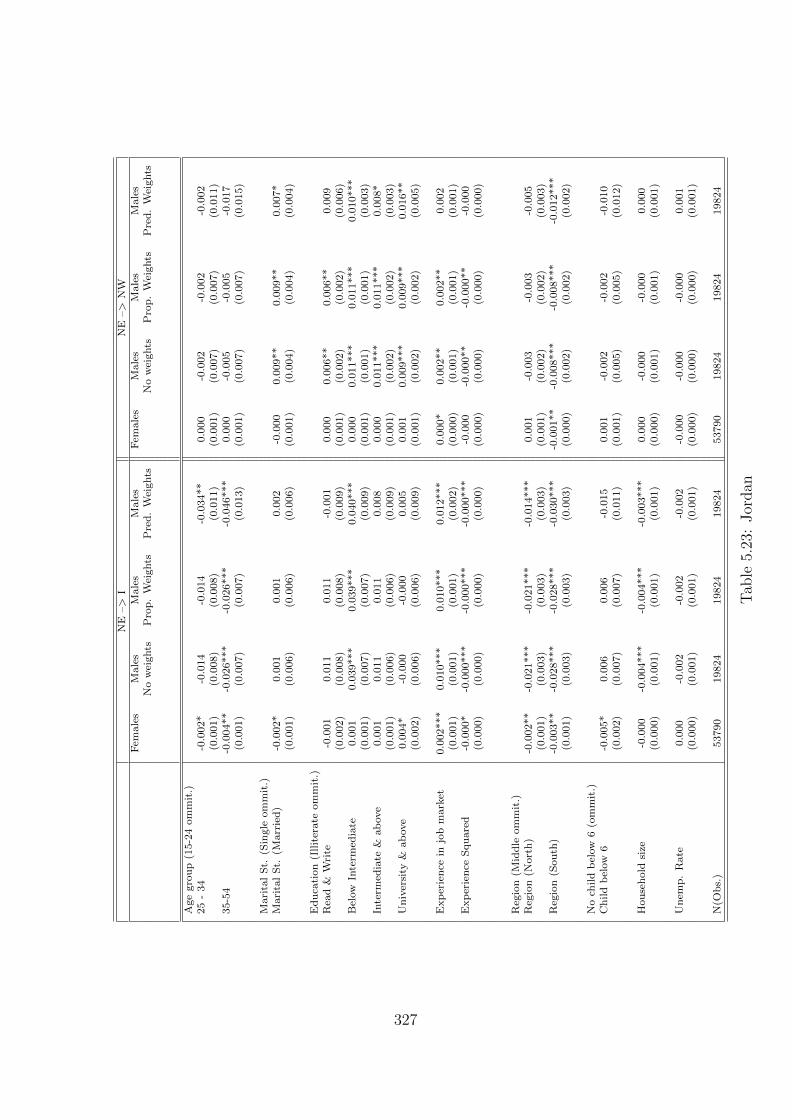
NE

–>

IN

E–>

NW

Fem

ale

sM

ale

sM

ale

sM

ale

sF

emale

sM

ale

sM

ale

sM

ale

sN

ow

eights

Pro

p.

Wei

ghts

Pre

d.

Wei

ghts

No

wei

ghts

Pro

p.

Wei

ghts

Pre

d.

Wei

ghts

Age

gro

up

(15-2

4om

mit

.)25

-34

-0.0

02*

-0.0

14

-0.0

14

-0.0

34**

0.0

00

-0.0

02

-0.0

02

-0.0

02

(0.0

01)

(0.0

08)

(0.0

08)

(0.0

11)

(0.0

01)

(0.0

07)

(0.0

07)

(0.0

11)

35-5

4-0

.004**

-0.0

26***

-0.0

26***

-0.0

46***

0.0

00

-0.0

05

-0.0

05

-0.0

17

(0.0

01)

(0.0

07)

(0.0

07)

(0.0

13)

(0.0

01)

(0.0

07)

(0.0

07)

(0.0

15)

Mari

tal

St.

(Sin

gle

om

mit

.)M

ari

tal

St.

(Marr

ied

)-0

.002*

0.0

01

0.0

01

0.0

02

-0.0

00

0.0

09**

0.0

09**

0.0

07*

(0.0

01)

(0.0

06)

(0.0

06)

(0.0

06)

(0.0

01)

(0.0

04)

(0.0

04)

(0.0

04)

Ed

uca

tion

(Illit

erate

om

mit

.)R

ead

&W

rite

-0.0

01

0.0

11

0.0

11

-0.0

01

0.0

00

0.0

06**

0.0

06**

0.0

09

(0.0

02)

(0.0

08)

(0.0

08)

(0.0

09)

(0.0

01)

(0.0

02)

(0.0

02)

(0.0

06)

Bel

ow

Inte

rmed

iate

0.0

01

0.0

39***

0.0

39***

0.0

40***

0.0

00

0.0

11***

0.0

11***

0.0

10***

(0.0

01)

(0.0

07)

(0.0

07)

(0.0

09)

(0.0

01)

(0.0

01)

(0.0

01)

(0.0

03)

Inte

rmed

iate

&ab

ove

0.0

01

0.0

11

0.0

11

0.0

08

0.0

00

0.0

11***

0.0

11***

0.0

08*

(0.0

01)

(0.0

06)

(0.0

06)

(0.0

09)

(0.0

01)

(0.0

02)

(0.0

02)

(0.0

03)

Un

iver

sity

&ab

ove

0.0

04*

-0.0

00

-0.0

00

0.0

05

0.0

01

0.0

09***

0.0

09***

0.0

16**

(0.0

02)

(0.0

06)

(0.0

06)

(0.0

09)

(0.0

01)

(0.0

02)

(0.0

02)

(0.0

05)

Exp

erie

nce

injo

bm

ark

et0.0

02***

0.0

10***

0.0

10***

0.0

12***

0.0

00*

0.0

02**

0.0

02**

0.0

02

(0.0

01)

(0.0

01)

(0.0

01)

(0.0

02)

(0.0

00)

(0.0

01)

(0.0

01)

(0.0

01)

Exp

erie

nce

Square

d-0

.000*

-0.0

00***

-0.0

00***

-0.0

00***

-0.0

00

-0.0

00**

-0.0

00**

-0.0

00

(0.0

00)

(0.0

00)

(0.0

00)

(0.0

00)

(0.0

00)

(0.0

00)

(0.0

00)

(0.0

00)

Reg

ion

(Mid

dle

om

mit

.)R

egio

n(N

ort

h)

-0.0

02**

-0.0

21***

-0.0

21***

-0.0

14***

0.0

01

-0.0

03

-0.0

03

-0.0

05

(0.0

01)

(0.0

03)

(0.0

03)

(0.0

03)

(0.0

01)

(0.0

02)

(0.0

02)

(0.0

03)

Reg

ion

(Sou

th)

-0.0

03**

-0.0

28***

-0.0

28***

-0.0

30***

-0.0

01**

-0.0

08***

-0.0

08***

-0.0

12***

(0.0

01)

(0.0

03)

(0.0

03)

(0.0

03)

(0.0

00)

(0.0

02)

(0.0

02)

(0.0

02)

No

child

bel

ow

6(o

mm

it.)

Child

bel

ow

6-0

.005*

0.0

06

0.0

06

-0.0

15

0.0

01

-0.0

02

-0.0

02

-0.0

10

(0.0

02)

(0.0

07)

(0.0

07)

(0.0

11)

(0.0

01)

(0.0

05)

(0.0

05)

(0.0

12)

Hou

seh

old

size

-0.0

00

-0.0

04***

-0.0

04***

-0.0

03***

0.0

00

-0.0

00

-0.0

00

0.0

00

(0.0

00)

(0.0

01)

(0.0

01)

(0.0

01)

(0.0

00)

(0.0

01)

(0.0

01)

(0.0

01)

Un

emp

.R

ate

0.0

00

-0.0

02

-0.0

02

-0.0

02

-0.0

00

-0.0

00

-0.0

00

0.0

01

(0.0

00)

(0.0

01)

(0.0

01)

(0.0

01)

(0.0

00)

(0.0

00)

(0.0

00)

(0.0

01)

N(O

bs.

)53790

19824

19824

19824

53790

19824

19824

19824

Tab

le5.

23:

Jor

dan

327

Chapter 6

A Structural Estimation of Labor

Market Frictions Using Data with

Measurement Error: Evidence from

Egypt and Jordan1

6.1 Introduction

Research on labor market dynamics of the MENA region and its policy implications

remains disturbingly limited and at its infant phase. With high persistent unemploy-

ment rates over the last decade, there has been an increasing urge to explore the

dynamics of these labor markets under the presence of search frictions awaiting to re-

solve the current paradox, where increasing GDP growth rates do not seem to create

enough jobs to absorb new labor market entrants. Pissarides (2002) shows that the

search equilibrium environment allows modeling an equilibrium in the labor market

1This paper has previously been circulated under a different title “Structural labor market transi-tions and wage dispersion in Egypt and Jordan”. The construction of spells has been modified, recentwaves of data sets are now used and recall/design measurement errors are now being considered. Theestimation methodology is also modified to allow for both right and left censoring. The novel idea ofthis paper is mainly based on my Masters thesis at the University of Paris 1 Pantheon-Sorbonne. Iwould like to thank my masters’ thesis supervisor Fabien Postel-Vinay as well as my PhD supervisorFrancois Langot for all the help and guidance. Microeconomics seminar Participants at the ETE mas-ters program (2009-2010) also provided valuable remarks. Comments and suggestions, at early stagesof this reasearch paper, from Ragui Assaad and Nicolas Jacquemet, are gratefully acknowledged.

328

in the presence of search frictions. Consequently, the time delay for an unemployed

worker to access a job or for a firm to fill an open vacancy, is possibly explained.

In his review of the search equilibrium literature, Launov (2006) shows that there

exists two main approaches to modeling search equilibrium on the labor market. This

classification basically depends on the way the nature of search frictions and the na-

ture of equilibrium wage setting are viewed. The first approach is to account for search

frictions in the form of incomplete information about the available vacancies, which

generates a time delay until the meeting/matching between the unemployed workers

and firms with vacancies takes place. Diamond (1982), Mortensen (1982) and Pis-

sarides (1985) adopted this approach. Wages are determined in this case through a

Nash bargaining process as long as the application of the Nash solution to the equilib-

rium wage determination is justified (Binmore, Rubinstein, and Wolinsky, 1986). The

second class of models assumes that search frictions result from workers’ incomplete

information about the offered wages. In this case workers receive take-it or leave-it

wage offers (one per period) and have the choice to either accept or reject the offer

before they can draw a new one. Early job search models adopted this approach that

was added later on to the search equilibrium framework by Diamond (1971), Albrecht

and Axell (1984) and Burdett and Mortensen (1998). Wages are hence determined in

these models via a wage posting game among employers.

Assessing the inflows and outflows of unemployment becomes possible using the

first approach where the transition rates can be obtained in function of labor mar-

ket tightness, workers’ search intensities..etc (Pissarides, 1990). Langot and Yassine

(2015,2015b) (Chapters 3 and 4) choose to adopt this approach in an attempt to un-

derstand the nature of the dynamics of the Egyptian labor market, in terms of whether

workers find jobs or not and how jobs are destroyed. This method however does not

allow to portray the quality of jobs and movements of workers up the job ladder since it

is less informative about on-the-job search and no endogenous wage offer distributions

can be obtained. Empirical applications are consequently very limited using the first

approach. In contrast, the second approach adopts a model with wage posting and

on-the-job search which solves for a unique endogenous wage offer distribution which

is a crucial feature that facilitates the estimation and the empirical application of the

329

model. This paper therefore chooses to focus on the second class of models.

These theoretical research efforts have been followed by a growing empirical lit-

erature dealing with the structural estimation of equilibrium search models to study

persistent wage and unemployment differentials. Mortensen and Pissarides (1999) show

that job and worker flows along with wage dispersion are the two main empirical phe-

nomena that enable labor market analysis via the search framework. Eckstein and

Van den Berg (2007) and Van Den Berg (1999) survey the empirical literature and

discuss most applications of these models. Bowlus (1997) studies gender wage differ-

entials, Bontemps, Robin, and Van den Berg (2000) discuss evidence of sectorial wage

differences, Bowlus, Kiefer, and Neumann (2001) analyze the transition from school

to work for young workers while Bowlus and Eckstein (2002) allow for discrimination

and skill differentials in their estimations. Finally, Ridder and Berg (2003) and Jolivet,

Postel-Vinay, and Robin (2006) provide cross-country comparisons of estimates from

equilibrium search models.

In this paper, a rudimentary partial equilibrium job search model is used to esti-

mate the structural labor market transitions between employment and non-employment

states. No previous attempts, to the best of my knowledge, were made to estimate job

search equilibrium models for the two MENA countries in question namely Egypt and

Jordan. Employment and non-employment spells are obtained from extracted synthetic

6-year panels using retrospective information available in the Egypt labor market panel

suvey (ELMPS) fielded in 2012 and the Jordan labor market panel survey fielded in

2010.

Jolivet, Postel-Vinay, and Robin (2006) estimate a similar partial equilibrium job

search model a la Burdett-Mortensen. They however allow for wage cuts when workers

move from one job to the other, refering to those as involuntary job moves. This paper’s

labor turnover model and estimation methodology resemble theirs except that it is not

possible to allow for wage cuts given the information available in the datasets used.

Jolivet, Postel-Vinay, and Robin (2006) also show the close correspondance between the

determinants of labor turnover and wage mobility, and the determinants of the cross-

sectional wage distribution. This correspondance is used in this paper to be able to

exploit the datasets available for the countries in question, (i) to provide a quantitative

330

measure of the search frictions and (ii) to test to what extent the model fits the data

i.e. reality and the particular nature of these developing countries’ labor markets.

The analysis in this paper adopts Bontemps, Robin, and Van den Berg (2000) two-

step semi-parametric estimation procedure. First, the accepted earnings distribution

is non-parametrically estimated. Second, these estimates are used to recover frictional

parameters using maximum likelihood techniques. Along with Mortensen (2003), Bon-

temps, Robin, and Van den Berg (2000) have also demonstrated that both heterogeneity

in firms’ productivity and search frictions are necessary to fit the wage distribution.

Although, this paper focuses on the labor supply side, this context is implicitly taken

into consideration to allow for a theoretical wage distribution that fits its empirical

counterpart.

Previous literature using the same or similar datasets such as Assaad, Krafft, and

Yassine (2015) (chapter 2 and Langot and Yassine (2015) (chapter 3) have shown

however that the retrospective information obtained from Egypt labor market panel

surveys (ELMPS) for instance, suffer from what is referred to as recall and design bias.

Following the same steps as in Yassine (no date) (chapter 5), the aggregate labor market

transition rates are corrected by estimating the measurement errors using auxiliary

information for each country to match true unbiased population moments (whether

transitions or stocks). These are then used to create readily-used longitudianl panel

weights for each individual spell dependent on the state occupied at the start and at

the end of the spell as well as its duration and the type of transition occuring after it

ends. Not only that the paper is used to study the labor market differentials between

the two MENA countries (Egypt and Jordan), it also aims at measuring to what extent

the estimated labor market frictional parameters can be biased due to measurement

error in retrospective accounts.

The analysis in this paper focuses on the labor market imperfections and provides

a quantitative measure of the importance of frictions for each country for a sample of

male private wage workers between 15 and 49 years of age in the year 2006 and 2004 for

Egypt and Jordan respectively. The frictional parameters are also examined among two

age-groups, namely “the youngs 15-24 years old” and “the olds 25-49 years old”. The

estimations are carried out using maximum likelihood techniques delivering frictional

331

transition parameters for each country, for the samples with and without longitudianl

correcting panel weights, as well as for two different age groups. Indeed, the data used

contains sufficient information on wages, labor markets states, durations and transitions

required to identify the model’s structural transition parameters. However, the major

advantage of using these labor market panel surveys (ELMPS and JLMPS) is that

they have similar questionnaires’ structures. This paper is therefore using homogenised

similar data for the two MENA countries. This allows for interesting intra and inter-

country comparisons.

The main findings of the paper can be summarized as follows. In general, the Jor-

danian labor market is more flexible than the Egyptian, especially among the younger

group of workers; job durations are relatively shorter. In contrast, Egyptian young

workers have shorter non-employment spells. In Egypt, the duration of remaining non-

employed declines with age; as one gets older (more precisely moves from the 15-24

years old group to the 25-49 years old group), job offers arrive at a faster rate. In

Jordan, however, non-employment durations get shorter for the old group of workers

and are shorter than that for the Egyptian old workers. Young Egyptian workers are

found to have the highest level of search frictions (κ1 estmates being the smallest),

relative to the older Egyptian workers and Jordanian workeres -both young and old.

This implies that the firms’ monopsony power in this trench of the Egyptian market is

the highestleading to low levels of salaries. Since small firms tend to pay lower wages,

a higher density of small sized firms is captured for the Egyptian market. This result

is confirmed by the empirical data. This paper also shows that correcting for the recall

and design bias in the used datasets matters significantly to the estimation of the job

destruction probabilities. The estimates of the index of search frictions is as a result

sensitive to this correction.

The rest of the paper is divided as follows. Section 2 overviews the data treatment

and the descriptive statistics of the analysis samples used. A model, along the lines of

chapters 3 and 5, is built to correct for the recall and design bias allowing to attribute

332

proportional weights2 to the micro-data to be able to use it the estimations. The third

section provides a description of the partial equilibrium job search model estimated.

Section 4 describes the estimation methodology, the empirical results obtained and

compares the extent and nature of search frictions when using or not using correcting

panel weights, across the three countries and across the different age groups. Section 5

concludes.

6.2 Data and Sampling

6.2.1 A Brief Description of the Samples

Data from Egypt and Jordan are used. The third rounds of the Egypt Labor Market

Panel Survey (ELMPS), fielded in 2012 and the Jordan Labor Market Panel Survey

(JLMPS) of 2010 are exploited. The surveys are nationally representative including

both detailed current employment and nonemployment information as well as labor

market histories that allow for an assessment of employment and nonemployment tran-

sitions and spells’ durations. The surveys elicit information on cross-sectional earned

wages and detailed individual characteristics. The major advantage of the two surveys

used, lies in the similarity between their questionnaires’ structures3. The datasets are

therefore closely homogenized and harmonized for the three countries allowing inter-

esting inter-country comparisons.

The analysis sample of this study consists of a cohort of private male wage workers,

between 15 and 49 years of age for each country. Using guidelines and assumptions from

Yassine (2014) (chapter 1), semi-annual employment/non-employment retrospective

trajectories have been extracted over a period of 6 years preceding the year of survey,

i.e. 2006-2012 for Egypt and 2004-2010 for Jordan.

Female workers are excluded to avoid gender wage differentials’ and labor force

participation issues. Female workers’ movements in and out of employment are likely

2Proportional weights are currently used for simplicity, assuming that all individuals making thesame type of transition in the same year mis-report retrospectively the same way. Further work isneeded to relax this assumption and to carry out the estimations using differentiated predicted weights,as in chapter 5.

3See chapter 1 for a detailed discussion of the structure of these surveys, the type of questionsused to survey the respondents and the way the answers are coded in the data.

333

to be driven by personal motives such as child birth and marriage. Moreover, since I rely

on retrospective information to create synthetic panel datasets, the sample is limited

to ages 15-49, to avoid backward attrition as discussed by (Yassine, 2014). This is

mainly done to avoid including in the analysis old groups of people that may not be

well representative in the retrospective panel since some old people might have been

alive back in 2006 and 2004 for Egypt and Jordan respectively but were not present to

be interviewed in the year of the survey. One of the aims of the paper is to capture,

if any, the differentials between the younger and older group of the sample in terms

of frictional transition parameters and wage dispersion. For this purpose, distinction

is made between two age group sub-samples, 15 to 24 years of age and 25 to 49 years

of age. The estimations are therefore re-run separately for each sub-sample for each

country.

Table 6.1 provides an overview of the descriptive statistics of the samples and sub-

samples used in the estimations. All durations are estimated in years and the wages are

in local currency rates. The wage distributions were observed to have very long tails.

To avoid the estimation procedure being sensitive to outliers in the wage data, the

lowest and highest 0.75% (for Egypt) and 1.5% (for Jordan) of the wage observations

in each sample and sub-sample are trimmed.

334

Egypt Jordan

ALL 15-24 years 25-49 years ALL 15-24 years 25-49 years

No. of individuals 7001 4001 3000 3218 1798 1420

Employed 4776 1999 2777 1683 577 1106Unemployed 2225 2002 223 1535 1221 314

Age 25.13 19.30 32.91 25.76 18.77 34.62(std. dev.) (8.35) (2.82) (6.81) (9.32) (2.79) (6.84)

Unemployed 31.78% 50.04% 7.43% 47.70% 67.91% 22.11%utoj 927 873 54 437 373 64

41.66% 43.61% 24.22% 28.47% 30.55% 20.38%Mean spell length 5.11 4.83 9.55 10.31 10.91 6.77(std. dev.) 3.13 (2.60) (6.21) (5.99) (6.04) (4.26)

Right Censored 1298 1129 169 1098 848 25058.34% 56.39% 75.78% 71.53% 69.45% 79.62%

Left Censored 1918 1712 206 1317 1033 28486.20% 85.51% 92.38% 85.80% 84.60% 90.45%

Employed 68.22% 49.96% 92.57% 52.30% 32.09% 77.89%jtoj 767 420 347 513 226 287

16.06% 21.01% 12.50% 30.48% 39.17% 25.95%Mean spell length 8.41 6.14 11.16 8.73 5.98 10.89(std. dev.) (6.06) (3.67) (7.15) (5.99) (3.52) (6.61)

jtou 318 186 132 225 69 1566.66% 9.30% 4.75% 13.37% 11.96% 14.10%

Mean spell length 10.03 6.55 14.94 11.91 6.71 14.21(std. dev.) (7.27) (3.35) (8.40) (7.85) (3.54) (8.14)

Right Censored 3691 1393 2298 945 282 66377.28% 69.68% 82.75% 56.15% 48.87% 59.95%

Left Censored 4405 1719 2686 1558 500 105892.23% 85.99% 96.72% 92.57% 86.66% 95.66%

Wage DistributionMin 108.33 100 120 52 48 60Max 8000 7000 12966.67 5720 4180 7870P10 403.24 400 433.33 150 150 150Median 864.5 842 900 250 250 270P90 1562 1542.67 2000 600 500 833.33P90/P10 3.87 3.86 4.62 4.00 3.33 5.56Skewness 3.49 3.47 5.81 5.51 6.09 4.90Kurtosis 23.49 23.98 49.76 35.74 42.78 28.97Mean 1006.09 972.6 1174.28 407.05 347.61 538.84(std. dev.) (709.15) (658.78) (1199.64) (664.13) (504.95) (1007.83)

a. Durations are expressed in years. These spells’ lengths account for left censored observations i.e. those spells whichstarted before 2006 (for Egypt) and 2004 (for Jordan). They exclude right censored observations.b. Wages are monthly wages expressed in local currencies.

Table 6.1: Descriptive Statistics

335

6.2.2 Creating Longitudinal Recall Weights

Since the structural estimations of the job search model rely mainly on duration

data, I was concerned by how biased the results might be if start and end dates of spells

are mis-reported or if some spells are even reported at all. The limitations and poten-

tial errors synthetic panel data, constructed from retrospective accounts, are subject

to, were discussed by previous literature working with the same data attempting to

build conclusions on the dynamics of the labor markets in the MENA region. Assaad,

Krafft, and Yassine (2015) (chapter 2) have provided detailed evidence on how different

labor market statuses, especially unemployment, are prone to misreporting over time,

comparing retrospective and contemporaneous data for the same individuals over time

using the Egypt Labor Market Panel Surveys (ELMPS) 1998, 2006 and 2012. In an

attempt to measure the impact of the new Egypt labor law implemented in 2004 on the

job finding and separation time series flows of the country, (Langot and Yassine, 2015)

(chapter 3) were concerned by the recall and design bias observed in the data. Even

with high quality collection methods and accurate cross-validated questions, the Egypt

labor market panel survey and retrospective information are subject to a memory bias

(recall error), where individuals tend to over-report their past employment statuses

and under-report their non-employment spells especially the short ones. The way the

survey is designed and questions are interpreted might have also contributed to what

(Langot and Yassine, 2015) refer to as a potential design bias in the data. Given the

very rich information obtained about the most recent employment/non-employment

vector versus relatively limited information about past trajectories, the observed un-

derestimation of separations and over-estimation of job findings as one goes back in

time is accentuated.

(Langot and Yassine, 2015) porposed a theoretical model to correct the aggregate

transition rates obtained from the retrospective data with the assumption that the

contemopraneous panel data transitions and stocks rates are the correct ones. In the

latter paper, this methodology has been adopted given that three waves of the Egypt

labor market panel survey 1998, 2006 and 2012 are available. To be able to correct

the aggregate transition rates obtained from the retrospective accounts of the ELMPS

2012, auxiliary information is therefore used from the contemporaneous information

336

(i.e. the unbiased information) obtained from the ELMPS 1998 and 2006 surveys. The

retrospective panels extracted for Jordan, given the similar structure of the survey’s

questionnaire, are biased as well due to the recall and design errors. The available

JLMPS 2010 is however the first and only round of the survey fielded in Jordan. Yas-

sine (no date) (chapter 5) proposed to derive auxiliary information on true unbiased

population stocks moments from comparable annual cross-sectional labor force surveys,

the Employent and Unemployment Surveys (EUS), conducted by the Jordanian depart-

ment of Statistics (DOS) as well as non-employment to employment job finding rates

and employment to non-employment separation rates for the years between 2007-2010,

from the annual Job Creation Surveys (JCS), to be able to identify the correction model

in this case.

Following the same steps as in chapter 5, the first step adopted in correcting the

recall and design bias observed in the data, is matching the stocks’ and transitions’

moments of the biased data with true auxiliary information to be able to estimate the

associated error terms to each type of transition on the aggregate level. Consequently,

the way the model is estimated differs between Egypt and Jordan, because of the dif-

ferences in the auxiliary data availability and the number of waves of Labor Market

Panel Survey fielded in the country. For both countries, the model is over-identified

and further work is needed to develop tests of fit for the model. The model is used to

structurally estimate, using a Simulated Method of Moments (SMM), a function repre-

senting the “forgetting rate” conditional on the individual’s state in the labor market.

Chapters 3 and 5 describe in details the setting of the model and the identification

strategy for each of the two countries using the relevant datasets.

The second step of the correcting technique is then distributing the estimated mea-

surement errors among the sample’s individual observations/transactions in the form of

micro-data weights, such that observations that are being under-reported take higher

weights and those over-reported take lower weights. This shows that it is sufficient

to have population (i.e. stocks) and transitions moments to correct over- or under-

reporting biases in retrospective data. Once the moments are matched on the aggregate

level, a measurement error for each type of transition at a point in time t is estimated.

This measurement error can then be attributed among the sample’s individual obser-

337

vations, reported for this specific type of transition in year t, in the form of micro-data

transitions weights per transition transaction per year. This can be done via two ways,

as explained in chapter 5: a simple proportional attributing method or a differentiated

predicting method. These two methods depend on whether one assumes if individuals

making the same transition in year t mis-report the same way or not.

For the sake of simplicity at this stage of the paper, the error terms are distributed

proportionally in the form of an adjustment factor (rilk(t − 1, t) among the sample’s

individuals depending on the type of transition lk the individual undergoes between

the years t − 1 and t, with lk = EE,EU,EI, UE,UU, UI, IE, II, IU . First, a total

correction factor is calculated for each type of transition lk (from state l in year t− 1

to k in year t). For a specific type of transition in a certain year, this is done by

dividing the corrected transition rate by the observed transition rate and multiplying

by the number of individuals who made this transition in that year. In simple words,

this measures by how much the observed biased transition rate in year t need to be

redressed on the aggregate level to obtain the true corrected rate. This can be written

formally as follows;

Rlk(t− 1, t) =λlk(t− 1, t)±Ψz

λlk(t− 1, t)× nlk(t− 1, t) (6.1)

where λlk(t − 1, t) is the transition rate from state l occupied in t − 1 to the state

k occupied in t. These rates are obtained by aggregating the expanded number of

individuals making the transition lk from the year t − 1 to year t in the constructed

retrospective panels and dividing by the stock of l in the year t− 14. n is the number

of individuals experiencing the transition lk from year t − 1 to year t and Ψz is the

associated error term estimated on the macro aggregate level (depending on the way

it was estimated for each country). An individual (rilk(t − 1, t)) adjustment factor is

then calculated to be the attributed weight to the micro-data transitions lk. This is

done here proportionally, i.e. assuming that all individuals mis-report the same way

and hence they are all equiprobable and get the same weight, if they make the same

4See chapter 1 for the way flows, such as job finding and separation rates, are calculated.

338

type of transition between the year t− 1 and the year t. This leads to :

rilk(t− 1, t) =1

nlk(t− 1, t)×Rlk(t− 1, t)

=λlk(t− 1, t)±Ψz

λlk(t− 1, t)(6.2)

Figures 6.1 and 6.2 show how these weights correct labor market flows and stocks

obtained form the longitudinal retrospective panel datastes.

The final step of the correction methodology would be how to use these weights in

the structural estimation of the job search model, which relies mainly on spell duration

data. For this purpose longitudinal panel weights for each spell are created, such that

the panel weight is the product of all the adjustment factors rjt from the start year till

end year of a given spell. The longitudinal panel weight for a given spell n of individual

i that starts in year t and ends in year T is therefore given by the following expression:

win =T∏t=t

rjti

Figure 6.3 uses the average job turnover indicators over a 6-year period for both

Egypt and Jordan that we obtain in table 6.1. It shows the weighted non-parametric

Kaplan-Meier smoothed job spell hazard rates for the overall samples of both countries

as well as by age groups. Although these estimates might not be very precise due

to the high percentage of censored observations in the samples, but they demonstrate

very interesting and obvious inter-country differences. It is noted that the Jordanian

labor market is more flexible than the Egyptian, especially among the younger group

of workers; job durations are shorter. These curves suggest a slight negative dura-

tion dependence in Egypt and in contrast a positive duration dependence in Jordan,

particularly among the old workers.

Figure 6.4 finally plots the non-parametric Kaplan-Meier estimates on the non-

employment spell smoothed hazard rates i.e. the job accession rates. These estimates

include both new labor market entrants and job re-accessions after a job separation.

Once again, different patterns in the duration dependence in both countries are ob-

339

.02

.04

.06

.08

2000 2002 2004 2006 2008 2010

Unemp rate (raw) Unemp rate (corrected)

National estimate of unemp rate (CAPMAS)

(a) Unemployment rate

0

.02

.04

.06

2000 2002 2004 2006 2008 2010

Job−to−Job (raw) Job−to−Job (corrected)

(b) Job-to-job transition rates

0

.05

.1

.15

.2

2000 2002 2004 2006 2008 2010

Non−employment−to−Job (raw) Non−employment−to−Job (weighted)

(c) Non-employment to Employment jobfinding rates

0

.01

.02

2000 2002 2004 2006 2008 2010

Job−to−non−employment (raw) Job−to− non−employment (weighted)

(d) Employment to non-employment sepa-ration rates

Figure 6.1: Corrected descriptive statistics for stocks and flows obtained using syntheticpanel data of ELMPS 2012, male workers in all sectors, ages 15-49 years old

.02

.04

.06

.08

.1

.12

.14

2000 2002 2004 2006 2008 2010

Unemp rate (raw) Unemp rate (corrected)

National estimate of unemp rate

(a) Unemployment rate

0

.02

.04

.06

2000 2002 2004 2006 2008 2010

Job−to−Job (raw) Job−to−Job (corrected)

(b) Job-to-job transition rates

0

.05

.1

.15

.2

2000 2002 2004 2006 2008 2010

Non−employment−to−Job (raw) Non−employment−to−Job (corrected)

(c) Non-employment to Employment jobfinding rates

0

.02

.04

.06

2000 2002 2004 2006 2008 2010

Job−to−non−employment (raw) Job−to− non−employment (corrected)

(d) Employment to non-employment sepa-ration rates

Figure 6.2: Corrected descriptive statistics for stocks and flows obtained using syntheticpanel data of JLMPS 2010, male workers in all sectors, ages 15-49 years old

340

0

.025

.05

.075

.1

0 10 20 30 40analysis time (years)

Egypt

(a) Overall sample

0

.025

.05

.075

.1

0 10 20 30 40analysis time (years)

Jordan

(b) Overall sample

0

.025

.05

.075

.1

0 10 20 30 40analysis time (years)

15−24 years old 25−49 years old

Egypt

(c) By age group

0

.025

.05

.075

.1

0 10 20 30 40analysis time (years)

15−24 years old 25−49 years old

Jordan

(d) By age group

Figure 6.3: Job spell hazard rates (job durations in years), male private wage workers,15-49 years of age

served. For Egypt, job accession rate is high at relatively short durations (i.e. early

years of the labor market career) then drops abruptly to remain constant at longer

durations. This negative duration dependence is observed for both young and old

Egyptian workers. In Jordan the pattern is different. In general, Jordanian workers

seem to access jobs later than their Egyptian peers (late labor market entrants)5. Job

accession rates are in general low for the 15-24 years old group, yet are relatively high

at shorter durations and reveal a negative duration dependence pattern. Positive du-

ration dependence is observed however for the old group of workers till it reaches the

peak at about 20 years then drops abruptly afterwards.

5It’s important to note here that in the construction of the non-employment spells, when theelapsed duration could not be deduced through the retrospective accounts, this is assumed to be thedate at which the individual turned 15 years old i.e. the minimum age to be considered in the analysissample.

341

0

.025

.05

.075

.1

0 10 20 30 40analysis time (years)

Egypt

(a) Overall sample

0

.025

.05

.075

.1

0 10 20 30 40analysis time (years)

Jordan

(b) Overall sample

0

.025

.05

.075

.1

0 10 20 30 40analysis time (years)

15−24 years old 25−49 years old

Egypt

(c) By age group

0

.025

.05

.075

.1

0 10 20 30 40analysis time (years)

15−24 years old 25−49 years old

Jordan

(d) By age group

Figure 6.4: Non-employment hazard rates (non-employment durations in years), maleprivate wage workers, 15-49 years of age

6.3 The Burdett-Mortensen Model

6.3.1 The environment

This section provides a description of the partial equilibrium job search model to

be estimated, along the lines of Burdett and Mortensen (1998) and Bontemps, Robin,

and Van den Berg (2000). Focus is made on the supply side that is populated by a

continuum of exante identical workers whose behavior is characterized by the standard

job search model with on-the-job search. These workers are risk-neutral agents who

maximize their expected present value of future income stream with infinite horizon;

m is the large number of these homogenous workers in the economy. It is assumed

that the worker can be in one of two states, employed or unemployed and u is the

number of unemployed. Workers are assumed to search for jobs both when employed

and when unemployed. In both cases the probability of receiving an offer is distributed

according to a standard poisson process where (λ0) is the arrival rate of job offers while

unemployed, and (λ1) when employed. φ is the reservation wage when unemployed,

whereas the wage earned w is the reservation wage when employed. When unemployed

342

a worker has utility flow given by b; this is assumed equal among workers and can be

interpreted as the value of leisure (or non-market time) or the level of unemployment

benefit per period net of search costs.

When employed, workers earn their wage w. There is no endogenous job destruction

deriving from productivity shocks, but δ is the exogenous probability that a job is

destroyed at every moment in time. Define κ0 = λ0/δ and κ1 = λ1/δ. κ1 is used

later on as a measure of the importance of search frictions in the market. Finally, let

F (w) represent the distribution of wages offered to workers and G(w) the distribution

of wages actually paid to (i.e. accepted by) the employed workers. The latter is the

earnings distribution.

6.3.2 Worker behavior

Given this framework, the present value of being unemployed, U , solves the contin-

uous asset pricing equation

ρU = b+ λ0(

∫ w

w

maxV (x), UdF (x)− U) (6.3)

where ρ is the common discount rate, V (w) is the lifetime utility that a worker

derives from working for a wage of w, w is the upper bound of the support of F and w

is the lowest posted wage (the lower support of F ) ; w = maxφ,wmin , where wmin

can be any institutional wage floor. This equation simply states that the opportunity

cost of unemployment, the left-hand side of 6.3, is equal to the sum of the value of

non-market time and the expected gain of finding an acceptable job, the right-hand

side of 6.3. Analogously, the present value of being employed at wage w, solves

ρV (w) = w + δ(U − V (w)) + λ1(

∫ w

w

maxV (x), V (w)dF (x)− V (w)) (6.4)

which consists of the current wage, the likelihood and value of becoming unemployed

(getting laid off) and the likelihood and value of receiving an alternative job offer. It

is obvious that the utility flow of the employed worker is assumed to be equal to his

343

current wage (i.e. w).

Since V (w) increases with w 6 and U is independant of it, there exists a reservation

wage φ such that the indifference condition V (w) = U . By Virtue of 6.3 and 6.4 and

integrating by parts, one obtains a formal definition of φ as follows:

φ = b+ (λ0 − λ1)

∫ w

φ

F (x)

ρ+ δ + λ1F (x)dx. (6.5)

Burdett and Mortensen (1998) shows that focusing on the limiting case of zero

discounting and setting ρ = 0, equation 6.5 can be re-written in the following simpler

form:

φ = b+ (κ0 − κ1)

∫ w

φ

F (x)

1 + κ1F (x)dx (6.6)

This equation defines the reservation wage φ as a function of the structural param-

eters of the model.

Equation 6.6 explains how the possibility on-the-job search affects the optimal

search strategy of an unemployed worker. If wage offers arrive more frequently when

unemployed than when employed (λ0 > λ1), the reservation wage φ exceeds the value

of non-market time b. In that case it is more rewarding to search while unemployed

and the worker rejects wage offers in the interval (b, φ), even though this might cause

a utility loss over the short run. When the arrival rate is independant of employment

status (λ0 = λ1), the worker is indifferent between searching while employed and while

unemployed. Any job that compensates for the foregone value of non-market time is

acceptable in this case and thus φ = b. If on-the-job search is not possible (λ1 = 0),

the expression in (6) reduces to the standard optimality condition. This discussion

is crucial for the interpretation of the model’s estimated parameters and is used in

explaining the estimation results over the next section.

6V ′(w) = 1ρ+δ+λ1F (w)

344

6.3.3 Steady-state stocks and flows

The equation of motion of unemployment in this economy is given by the difference

between the inflow and the outflow of the stock. It therefore follows that in steady

state,

δ(m− u) = λ0[1− F (φ)]u (6.7)

Since no worker would be willing to accept a wage lower than the reservation wage,

F (φ) is therefore equal to zero. This implies using further manipulations that the

equilibrium unemployment rate is as follows:

u

m=

δ

δ + λ0

=1

1 + κ0

, (6.8)

Using an analogous argument the steady-state earnings distribution G can be de-

rived. This represents the cross-sectional wage distribution of currently employed work-

ers, associated with a given wage offer distribution F . Given the initial allocation of

workers to firms, the number of workers employed receiving a wage no greater than w

is G(w)(m− u); the evolution of this stock over time is therefore

dG(w)(m− u)

dt= λ0F (w)u− δ + λ1[1− F (w)]G(w)(m− u), (6.9)

The outflow (second term of the right-hand side of equation 6.9) is simply equal to

the sum of workers previously holding a job that has been destroyed (i.e. laid off, losing

their job due to a demand shock) and those who find a better opportunity (receiving

an offer greater than w) and hence quit their old job. The inflow consists of those

workers who are already unemployed and receive an offer greater than φ but still less

than w (the first term on the right-hand side of 6.9). In a steady state, these flows

should be equal. A structural relationship between the distribution of wages actually

paid to employed workers and the distribution of wages offered can therefore be derived

as follows:

345

G(w) =F (w)

δ + λ1[1− F (w)]· λ0u

m− u(6.10)

=F (w)

1 + κ1[1− F (w)]

⇔

1− F (w) =1−G(w)

1 + κ1G(w)

for all w on the common support of F and G. Since workers tend to move up

the wage range over time, the earnings distribution lies to the right of the wage offer

distribution, or more formally, G first-order stochastically dominates F as F (w) −

G(w) ≥ 0 for all w and κ1 ≥ 0. The discrepancy between the earnings and wage offer

distributions depends on κ1 which is equal to the expected number of wage offers during

a spell of employment (which may consist of several consecutive job spells) and can

be thought of a relative measure of competition among firms for workers. With g(w)

and f(w) being the densities of the corresponding cumulative distributions, it is also

possible to re-write the above structural relationship between the earnings and offered

wages as in equation 6.11.

f(w) =1 + κ1

[1 + κ1G(w)]2g(w) (6.11)

The model also allows to predict the average size of a firm l(w|φ, F ), in equation

6.12, offering a wage w given φ and F . This specifies the steady state number of workers

available to a firm offering a particular wage conditional on the wage offered by other

firms (i.e. F ) and the workers’ reservation wage φ, given uniform random sampling of

firms. l(w|φ, F ) is increasing in w and continuous on the support of the distribution F .

l(w|φ, F ) =g(w)

f(w)(m− u) (6.12)

⇔ l(w|φ, F ) =[1 + κ1G(w)]2

1 + κ1

(m− u)

346

6.4 Estimation

6.4.1 The Likelihood Function

In the analysis sample, individuals are sampled from the stock of nonemployed and

employed workers, rather than the flow. The contribution of an individual’s spell to

the likelihood function therefore depends on the state he/she is in at the year t = 0, i.e

2006 for the Egyptian sample and 2004 for the Jordanian. A binary variable indicates

the state of the agent in year t = 0, where unemployed workers take 0 and employed

1. Only the first spell that is in progress at the date t = 0 when the individuals are

sampled, is used. Information on subsequent spells are not used. Individuals who were

self-employed or employed by the government for some period during the time span

of the 6-year observation period are dropped. The behaviour of public and non-wage

workers as well as their employers are likely to differ to a great extent from the behavior

explained by the model. It is also important to note that no distinction is made between

unemployed and out of the labor force. The empirical counterpart of the theoretical

state of unemployment in the model is therefore nonemployment; this includes both

the unemployed as well as the non-participants.

Some spells might have started before the date of sampling t = 0. These spells are

left censored and are denoted by an indicator cil with i = 0, 1. An elapsed duration til

(with i = 0, 1) is therefore defined as the duration from the moment a spell started until

the sampling date. For individuals who ever worked, the elapsed date is deduced from

the retrospective accounts of the surveys. For individuals who never worked, if the spell

started before the year t = 0 amd the elapsed date is not provided by the retrospective

questions of the survey, this is assumed to be the date at which the individual turns 15

years old (which is the minimum age to be considered in our sample). Right-censored

observations are those spells in progress beyond the observation period. These are

denoted by the indicator cir, with i = 0, 1. The duration from the sampling date until

the moment at which the spell ends is defined as the residual duartion tir. The total

duration of an individual’s spell ti is therefore the sum of the elapsed til and residual

tir durations.

For each worker in the sample, the earned wage; denoted by w, is observed. Since

347

wages are not available in the retrospective information obtained from the ELMPS and

the JLMPS, only the cross-sectional wages’ distributions of 2012 and 2010 in Egypt

and Jordan respectively, are used as a proxy for all wage purposes in the model 7

About the distribution of the spells’ durations, it is known that at a certain time

ti after the start of the spell, a renewal of states (a transition) takes place. Since the

backbone process of the model is Poisson, the waiting time between any two adjacent

events is then exponentially distributed with parameter θ. Renewal probability for

Poi(θ) is shown to be equal to θ (see Lancaster (1990)). The appropriate density for

the spells’ durations can therefore be defined as follows:

f(ti) = θe−θti (6.13)

For the unemployed agents, the corresponding Poisson rate is just λ0. For the employed

ones, the Poisson rate is a sum of transition intensities to either unemployment δ or a

better-paid job λ1F (w) ,i.e. θ = δ + λ1F (w).

To complete the formulation of the individual contributions to the likelihood one

notes that:

• For Unemployed: Equilibrium probability of sampling an unemployed agent

is given by um

= δδ+λ

= 11+κ0

. In case an unemployment-to-job (utoj) transition

is observed, the offered wage and the value of the wage offer density f(w0) are

known and can be recorded.

• For Employed: Equilibrium probability of sampling an agent who earns wage w

is g(w)λ0/(δ+λ0) = g(w)κ0/(1+κ0). The model allows for two types of transitions

from employment: employment to unemployment (jtou) and job-to-job transition

(jtoj). The probabilities of renewal to unemployment and to another job are

Pr(j → u) = δ/(δ+λ1F (w)) and Pr(j → j) = λ1F (w)/(δ+λ1F (w)) respectively.

7This should not be a strong assumption. In the estimation, wages are needed to obtain the earnedwages density. This is done for the unemployed who have acquired a job at the end of their spell orfor the employed who have switched jobs. The cross-sectional years represent the last year of a 6-yearpanel observation period. In developing countries such as Egypt and Jordan, the occurence of multiplespells over a period of 6 years is not very common. The wage observed by the end of the observationperiod is therefore most likely the wage accepted by the end of a recorded individual’s spell.

348

For both the employed and the unemployed, an incompletely observed spell duration

(i.e. a right censored spell duration) is taken into consideration where renewal proba-

bilities are dropped and the density is replaced by the survivor function.

With this, the likelihood functions of an unemployed individual L0 and of an em-

ployed individual L1 become

L0 =λ2−c0r−c0l

0

1 + κ0

exp−λ0 × t0f(w)1−c0r (6.14)

L1 =κ0

1 + κ0

g(w)[δ + λF (w)]1−c1l exp−[δ + λ1F (w)](t1)× [ λ1F (w)

δ + λ1F (w)]v

× [δ

δ + λ1F (w)]1−v1−c1r

(6.15)

where v = 1, if there is a job-to-job transition,and 0 otherwise.

Since labor force surveys are being exploited, the theoretical wage offer distribution

and density functions are unknown. No analytical solution for F (w) is available. A

“nonparametric two-step procedure” is therefore adopted as proposed by (Bontemps,

Robin, and Van den Berg, 2000) for the estimation of the structural parameters.

1. On the first step, the non-parametric estimates of G(w) and g(w) are computed,

using a gaussian kernel estimator for the density g(w) and the empirical cumula-

tive distribution for G(w). Let G(w) and g(w) denote such estimates. Conditional

on κ1, consistent estimates of F and f are

F =1− G(w)

1 + κ1G(w)

and

f(w) =1 + κ1

[1 + κ1G(w)]2g(w)

2. F and f are then replaced in the likelihood function by the preceding expressions

349

to be able to obtain a baseline set of parameter estimates λ0, λ1, δ and κ1 by

maximizing the sample log-likelihood function separately for each country and for

each age agroup. Since one of the aims of this paper is to test to what extent the

search frictions parameters’ estimates might be biased due to recall and design

bias, the estimation for each sample (or sub-sample) is conducted twice, with and

without the created longitudinal panel recall weights.

6.4.2 Empirical Results

Egypt Jordan

Raw Data With panel weights Raw Data With panel weightsAllλ0 0.173 0.173 0.0885 0.0916

[0.161,0.184] [0.162,0.184] [0.0810,0.0961] [0.0846,0.0985]

λ1 0.18 0.171 0.171 0.187[0.163,0.197] [0.152,0.191] [0.154,0.188] [0.166,0.208]

δ 0.106 0.131 0.0533 0.0768[0.0986,0.113] [0.119,0.143] [0.0485,0.0581] [0.0698,0.0837]

κ1 1.698 1.305 3.208 2.435[1.518,1.878] [1.120,1.490] [2.796,3.620] [2.10,2.77]

15-24 years

λ0 0.189 0.191 0.0793 0.0787[0.176,0.202] [0.179,0.202] [0.0717,0.0870] [0.0716,0.0859]

λ1 0.267 0.262 0.328 0.401[0.236,0.299] [0.221,0.302] [0.283,0.373] [0.339,0.463]

δ 0.178 0.224 0.0847 0.117[0.164,0.192] [0.200,0.248] [0.0743,0.0950] [0.102,0.131]

κ1 1.500 1.170 3.872 3.427[1.303,1.697] [0.951,1.388] [3.185,4.560] [2.768,4.068]

25-49 years

λ0 0.158 0.15 0.204 0.212[0.130,0.186] [0.116,0.185] [0.164,0.244] [0.180,0.244]

λ1 0.151 0.144 0.133 0.139[0.128,0.174] [0.121,0.166] [0.114,0.152] [0.117,0.160]

δ 0.0395 0.0448 0.0366 0.0538[0.0342,0.0447] [0.0373,0.0524] [0.0313,0.0419] [0.0464,0.0612]

κ1 3.823 3.214 3.634 2.584[3.084,4.561] [2.462,3.967] [2.925,4.343] [2.071,3.096]

Table 6.2: Estimation Results

This section presents in table 6.2 the estimation results obtained for each country

with and without the longitudinal panel recall weights. Generally among all the samples

and sub-samples, the estimates for λ0 and λ1 are robust. Almost the same results are

350

obtained whether the recall weights are being used or not. The panel weights however

play a crucial role in the estimation of the job destruction parameter δ and consequently

the search frictions index κ1. The job destruction estimates are significantly under-

estimated if one does not take into consideration the recall and design bias in the data.

Conclusions about the magnitude of search frictions can therefore be mislead. With

higher job destruction rates, the level of search frictions is higher driving the estimates

of κ1 to be significantly smaller after correction. It’s important to highligh here that

the estimations of the frictional parameters in this paper are obtained using annual

durations over a 6-year observation period. That being said, these rates are relatively

low when compared to other countries’ estimations reflecting the rigidity of these labor

markets.

Examining the results obtained from the Egyptian sample, the arrival rate of ac-

ceptable wage offers when unemployed is found to be significantly lower than when

employed for the young workers. For this young group of workers, searching on the job

is more rewarding than searching when unemployed. Interestingly, their reservation

wage φ is extremely low to the extent that it might be lower than the non-market time

b. Young Egyptian workers do however have a higher rate of finding jobs, whether

unemployed or employed, than the older workers. For the older group 25-49 years,

however, the difference between searching for a job when unemployed or employed be-

comes nil. Their reservation wage φ is relatively higher but just as high as the foregone

value of the non-market time. In Jordan, the pattern is slightly similar except that as

it has been shown in the descriptive statistics, Jordanians access jobs later than the

Egyptians. This could possibly be explained by Jordanians spending more years in

education (i.e. non-participation) than Egyptians. The rate of arrival of acceptable

wage offers when unemployed for the old group (25-49 years old) is much higher (more

than double) than that of the youngs. Yet, the same pattern applies as one compares

the λ0 and λ1. Again for the youngs, it is more worth it to search on-the-job than when

unemployed. The situation for the unemployed ameliorates as one gets older, where λ0

exceeds λ1. The reservation wage of this group is higher than the value of non-market

time.

According to these results, the estimated average duration of non-employment in

351

Egypt is 5.7 years and 11 years in Jordan. It’s crucial to note here that the empirical

counterpart of the unemployment state in the theoretical model is non-employment.

These durations of non-employent therefore include years of inactivity as well, which

might be the reason why these durations do seem lengthy. The non-employment dura-

tion varies by age group where in Egypt the young workers might take up to 5 years

to access a job while older workers can stay up to 6.7 years. It’s very interesting that

for Jordan it’s the other way around. Older unemployed agents in Jordan only take

up to 4.7 years to access jobs, while the young unemployed agents can stay trapped

(voluntarily in case of education) in non-employment up to 12 years.

In both countries, the young group of workers experience more job-to-job transitions

(i.e. more churning in this market), with the young Jordanians being the most mobile.

The average duration (for the overall sample) of an employment relationship terminated

by a job-to-job transition is almost the same for both countries, of about 5.3-5.8 years.

The estimated parameters for the age group sub samples however show that much of

the churning occurs in both countries among the young aged groups. That’s when the

on-the-job search activity is relatively high. As an individual grows older, the λ1 rate

slows down to almost the half in Egypt and the third in Jordan.

The very rigid and immobile nature of these MENA region countries becomes even

confirmed as one examines the rate at which jobs are being destroyed. Unsurprisingly,

the rate at which a job is destroyed for an individual of age 15-24 years old is signifi-

cantly higher than that of a worker aged 25-49 years. Generally, the δ estimates, even

after correction from the measurement error, are strikingly low. The extent to how

measurement errors are able to bias our estimates become obvious as we compare the

weighted and unweighted average duration of a job ending with a separation. Indeed,

estimates of the job destruction parameters become significantly distorted when the

recall and design bias is ignored.

In general the estimated parameters are very low, reflecting the rigidity of these

labor markets. One might think that this might be partly artificial due to the fact

that all spells are truncated from below at six months8. These parameters would be

in that case biased downwards. In a non-truncated sample, the estimated parameter

8See chapter 1 for a discussion on the questionnaires and the data recorded by the enumerators.

352

converges to the true parameter 1/E(d), where d is a variable of observed durations

d1, d2, d3....dn of n individuals. When the sample is truncated, the biased parameter

would converge to 1/E(d|d ≥ D), where D is the duration below which the spells are

truncated. By how much the estimated parameter in that case would be biased mainly

depends on the probability of having durations that are below D, i.e. in our case

below six months. If this probability is very small, which is thought to be the case

in Egypt and Jordan given their labor market institutional framework as well as their

employment culture (chapter 1), the difference between the estimated parameter using

truncated and non-truncated spells would be negligeable.

In addition to the transition parameters of the model, table 6.2 provides estimates

of the “summary index of search frictions”κ1 = λ1/δ. This index gives a measure of the

speed at which workers climb the wage ladder, as well as the average number of offers

received in the time interval before the next worker becomes unemployed. One notes

that the two labor markets suffer from high levels of search frictions with relatively

low estimates of κ1. This is particularly true for the young Egyptian private waged

workers. It is also important to note that the significant difference in the magnitude

of these indices when weighted and unweighted originates mainly from the differences

between the corrected and unncorrected delta. Again, this confirms the importance

of correcting the data before building up conclusions on these labor markets since

estimates of frictional parameters in this case can be misleading and over-estimated as

in the case of the κ1. Assuming an equal opportunity of receiving better offers during

the year, young workers in Egypt receive more job offers during the year than their

older peers, but the opposite is true in Jordan.

Moreover, the theoretical model shows that the distribution of earned wages G(w)

first-order stochastically dominates F (w). The extent of this phenomenon depends

on the magnitude κ1. It’s simply a measure of inter-firm competition on the labor

market. If κ1 tends to zero, this means that λ1 tends to zero, meaning that employed

workers never get higher job values than what firms are offering them. In simple

words, it means that once a worker draws from F (w) (i.e. accepts a job), he/she

actually gets stuck there since it’s very unlikely to find a better job with a better

offer. G(w) becomes confounded then with F (w) and the workers tend to accept what

353

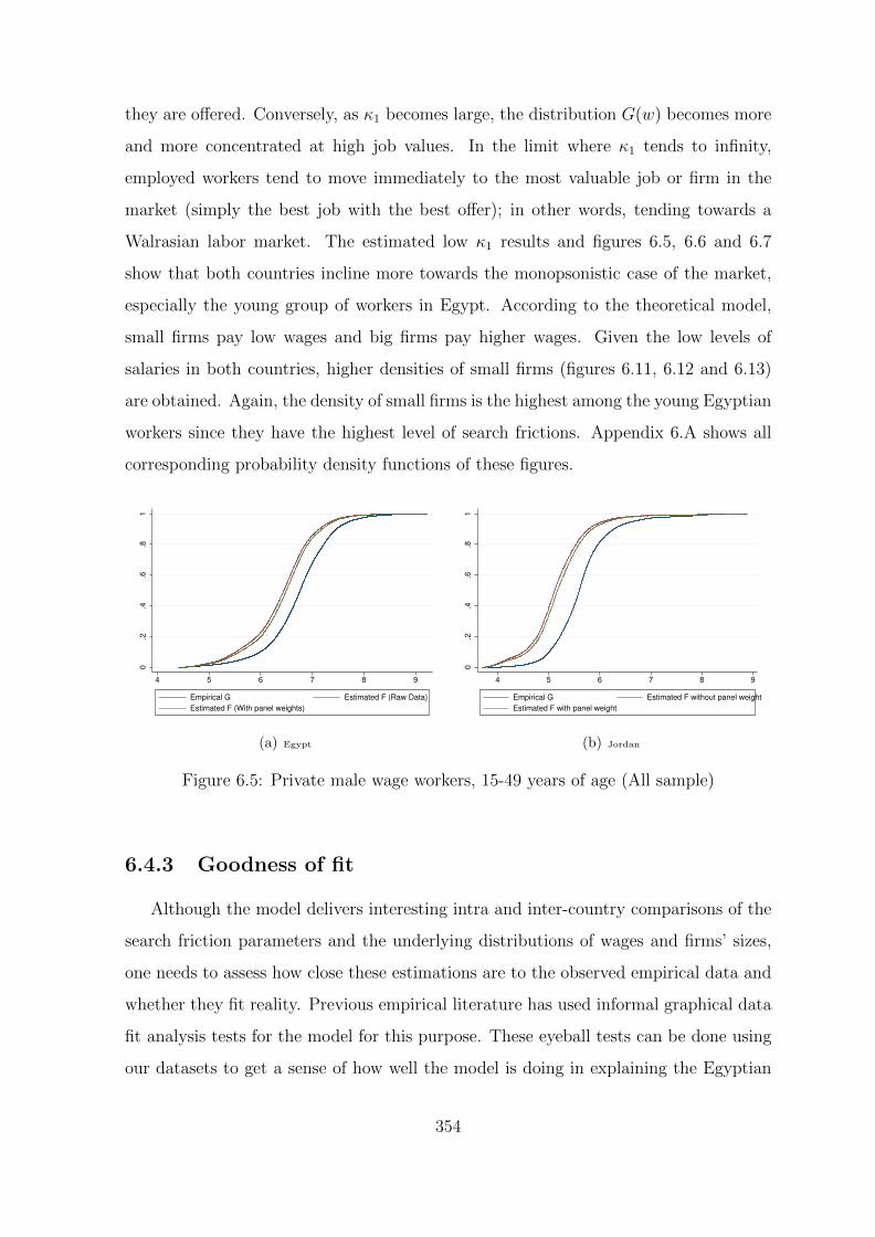
they are offered. Conversely, as κ1 becomes large, the distribution G(w) becomes more

and more concentrated at high job values. In the limit where κ1 tends to infinity,

employed workers tend to move immediately to the most valuable job or firm in the

market (simply the best job with the best offer); in other words, tending towards a

Walrasian labor market. The estimated low κ1 results and figures 6.5, 6.6 and 6.7

show that both countries incline more towards the monopsonistic case of the market,

especially the young group of workers in Egypt. According to the theoretical model,

small firms pay low wages and big firms pay higher wages. Given the low levels of

salaries in both countries, higher densities of small firms (figures 6.11, 6.12 and 6.13)

are obtained. Again, the density of small firms is the highest among the young Egyptian

workers since they have the highest level of search frictions. Appendix 6.A shows all

corresponding probability density functions of these figures.

0.2

.4.6

.81

4 5 6 7 8 9

Empirical G Estimated F (Raw Data)

Estimated F (With panel weights)

(a) Egypt

0.2

.4.6

.81

4 5 6 7 8 9

Empirical G Estimated F without panel weight

Estimated F with panel weight

(b) Jordan

Figure 6.5: Private male wage workers, 15-49 years of age (All sample)

6.4.3 Goodness of fit

Although the model delivers interesting intra and inter-country comparisons of the

search friction parameters and the underlying distributions of wages and firms’ sizes,

one needs to assess how close these estimations are to the observed empirical data and

whether they fit reality. Previous empirical literature has used informal graphical data

fit analysis tests for the model for this purpose. These eyeball tests can be done using

our datasets to get a sense of how well the model is doing in explaining the Egyptian

354

0.2

.4.6

.81

4 5 6 7 8 9

Empirical G Estimated F (Raw Data)

Estimated F (With panel weights)

(a) Egypt

0.2

.4.6

.81

4 5 6 7 8 9

Empirical G Estimated F without panel weight

Estimated F with panel weight

(b) Jordan

Figure 6.6: Private male wage workers, 15-24 years of age

0.2

.4.6

.81

4 6 8 10

Empirical G Estimated F (Raw Data)

Estimated F (With panel weight)

(a) Egypt

0.2

.4.6

.81

4 5 6 7 8 9

Empirical G Estimated F without panel weight

Estimated F with panel weight

(b) Jordan

Figure 6.7: Private male wage workers, 25-49 years of age

and Jordanian labor markets.

Following Jolivet, Postel-Vinay, and Robin (2006), the cdf of wages accepted by

workers who were just hired from unemployment can be used as a direct estimator

F 0(.) of the wage offers sampling estimated sampling distribution F (.). Empirically,

this direct estimator confirms the first stochastic dominance of the earnings distribution

over the offered wages as suggested in the theoretical model, for the overall sample and

the young age groups. The wage distributions however get slightly distorted for the

old Egyptian age group, probably due to the small number of observations used in the

non-parametric estimation. Figure 6.10 still plots the empirical F, of the old Egyptian

workers however, to get at least an idea of the level of F . The predicted theoretical

F (.) obtained using the maximum likelihood estimate of κ1, is then compared to the

355

0.2

.4.6

.81

4 5 6 7 8 9

F_unemployed Estimated F (Raw Data)

Estimated F (With panel weights)

(a) Egypt

0.2

.4.6

.81

2 4 6 8 10

Empirical F from new hires Estimated F without panel weight

Estimated F with panel weight

(b) Jordan

Figure 6.8: Private male wage workers, 15-49 years of age (All sample)

observed F 0(.) obtained from the cross-sectional wages’ distribution of workers who

were just hired from non-employment in the ELMPS 2012, JLMPS 2010 and TLMPS

2012.

F (ω; κ1) =(1 + κ1)G(ω)

1 + κ1G(ω)(6.16)

In general, the model’s predicted wage offer distributions are close to their empirical

estimators in both countries Egypt and Jordan and for all age groups, except for the

Egyptian old group of workers. As figures 6.8, 6.9 and 6.10 are scrutinized carefully

though, it is found that the model is doing much better in replicating reality in the

Jordanian labor market. Only the lowest 10-20% of the wage distributions are not

perfectly captured. For Egypt, however, this is only true for the lowest 50% of the

wage distributions and the highest wages in the distribution.

The availability of a categorized empirical distribution of the sizes of firms in the

data makes it possible to compare in figures 6.11, 6.12 and 6.13 the empirical and

theoretical (l(w)) distributions of firms’ sizes in these labor markets. These comparisons

confirm the above discussion about the high peaks and concentrations in the densities

of small sized firms in these countries. This phenomenon is confirmed by the empirical

histograms of the categories of firms’ sizes. In general, the theoretical model is capturing

the overall picture of the labor markets, both Egypt and Jordan. It might be however

356

0.2

.4.6

.81

4 5 6 7 8 9

F_unemployed Estimated F (Raw Data)

Estimated F (With panel weights)

(a) Egypt

0.2

.4.6

.81

2 4 6 8 10

Empirical F from new hires Estimated F without panel weight

Estimated F with panel weight

(b) Jordan

Figure 6.9: Private male wage workers, 15-24 years of age

0.2

.4.6

.81

4 6 8 10

F_unemployed Estimated F (Raw Data)

Estimated F (With panel weight)

(a) Egypt

0.2

.4.6

.81

2 4 6 8 10

Empirical F from new hires Estimated F without panel weight

Estimated F with panel weight

(b) Jordan

Figure 6.10: Private male wage workers, 25-49 years of age

357

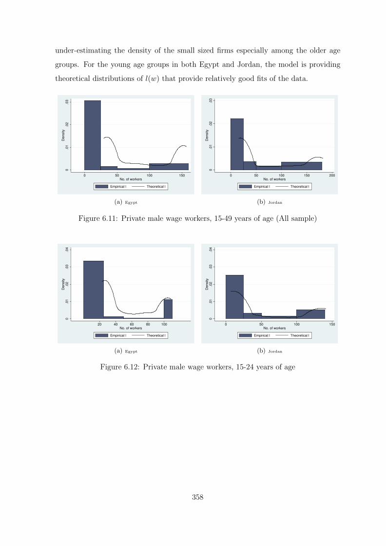
under-estimating the density of the small sized firms especially among the older age

groups. For the young age groups in both Egypt and Jordan, the model is providing

theoretical distributions of l(w) that provide relatively good fits of the data.

0.0

1.0

2.0

3D

ensity

0 50 100 150No. of workers

Empirical l Theoretical l

(a) Egypt

0.0

1.0

2.0

3D

ensity

0 50 100 150 200No. of workers

Empirical l Theoretical l

(b) Jordan

Figure 6.11: Private male wage workers, 15-49 years of age (All sample)

0.0

1.0

2.0

3.0

4D

ensity

20 40 60 80 100No. of workers

Empirical l Theoretical l

(a) Egypt

0.0

1.0

2.0

3.0

4D

ensity

0 50 100 150No. of workers

Empirical l Theoretical l

(b) Jordan

Figure 6.12: Private male wage workers, 15-24 years of age

358

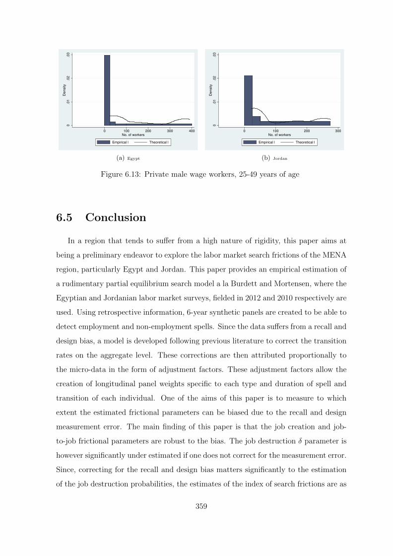
0.0

1.0

2.0

3D

ensity

0 100 200 300 400No. of workers

Empirical l Theoretical l

(a) Egypt

0.0

1.0

2.0

3D

ensity

0 100 200 300No. of workers

Empirical l Theoretical l

(b) Jordan

Figure 6.13: Private male wage workers, 25-49 years of age

6.5 Conclusion

In a region that tends to suffer from a high nature of rigidity, this paper aims at

being a preliminary endeavor to explore the labor market search frictions of the MENA

region, particularly Egypt and Jordan. This paper provides an empirical estimation of

a rudimentary partial equilibrium search model a la Burdett and Mortensen, where the

Egyptian and Jordanian labor market surveys, fielded in 2012 and 2010 respectively are

used. Using retrospective information, 6-year synthetic panels are created to be able to

detect employment and non-employment spells. Since the data suffers from a recall and

design bias, a model is developed following previous literature to correct the transition

rates on the aggregate level. These corrections are then attributed proportionally to

the micro-data in the form of adjustment factors. These adjustment factors allow the

creation of longitudinal panel weights specific to each type and duration of spell and

transition of each individual. One of the aims of this paper is to measure to which

extent the estimated frictional parameters can be biased due to the recall and design

measurement error. The main finding of this paper is that the job creation and job-

to-job frictional parameters are robust to the bias. The job destruction δ parameter is

however significantly under estimated if one does not correct for the measurement error.

Since, correcting for the recall and design bias matters significantly to the estimation

of the job destruction probabilities, the estimates of the index of search frictions are as

359

a result sensitive to this correction. These are consequently smaller reflecting higher

search frictions in these labor markets.

Overall, the Jordanian labor market is found to be more flexible than the Egyptian,

especially among the younger group of workers; job durations are relatively shorter.

In contrast, Egyptian young workers have shorter non-employment spells. In Egypt,

job offers arrive at a faster rate for the non-employed as they get older, however in

Jordan, it is the reverse. Non-employment durations for the Jordanian old group of

workers is shorter than that for the Egyptian old workers. This shows that Jordanian

workers tend to access jobs later than their Egyptian peers, probably due to longer

years of schooling. Young Egyptian workers are found to have the highest level of

search frictions (κ1 estmates being the smallest), relative to the older Egyptian workers

and Jordanian workeres - both young and old. This implies that the firms’ monopsony

power in this trench of the Egyptian market is the highest leading to low levels of

salaries. Since small firms tend to pay lower wages, a higher density of small sized

firms is captured for the Egyptian market. This result is confirmed by the empirical

data.

This analysis is likely to contribute to the new emerging literature dealing with

the MENA region labor markets. To the best of my knowledge, it represents the first

attempt to estimate the dynamics and search frictions of these labor markets in a

framework of equilibrium job search models. Since a lot of nature-specific aspects, such

as informality, awaiting queues for the public sector and non-wage mobility determi-

nants, need to be taken into consideration, it’s likely that this paper’s estimates might

be slightly overestimating rigidity by limiting the analysis to only the private wage

employment sector of these labor markets.

Extensions: Further work is needed to re-run estimations carried out in this chap-

ter, using the differentiated predicted weights built in chapter 5. This is likely to affect

the results since the sample limits to private wage workers, who are likely to mis-report

differently than public and non-wage workers for instance. Moreover, this becomes par-

ticularly valuable as the distinction between the two age groups is made. The youngs

and the olds do not simply mis-report in the same way. Moreover, since the proposed

correction has a significant impact on the final estimates of the BM parameters, more

360

investigation is needed to expand on the role of the parametric function assumed for the

decay of information as one goes back in time, especially that differences are possible

between the way the loss of memory and accuracy occurs in Egypt and Jordan. The

over-identification of the model should allow for the development of tests of fit for the

model. Finally, since the available data allows the distinction between the different

employment sectors, namely public, informal and formal wage work, it should be in-

teresting to extend the model as has been done Meghir, Narita, and Robin (2012) and

Bradley, Postel-Vinay, and Turon (2013), and estimate the frictional parameters as the

market is segmented into different sectors. The comparison between the simple and

extended Burdett Mortensen parameters might reveal interesting conclusions relevant

to the particular nature of the developing countries in question characterized by the

presence of oversized public sectors and unreglauted private informal jobs9.

9See chapter 1 for a survey on the labor market institutional framework in Egypt and Jordan.

361

References

Albrecht, J. W., and B. Axell (1984): “An equilibrium model of search unem-

ployment,” The Journal of Political Economy, pp. 824–840.

Assaad, R., C. Krafft, and C. Yassine (2015): “Comparing Retrospective and

Panel Data Collection Methods to Assess Labor Market Dynamics,” Discussion pa-

per, Economic Research Forum, Cairo.

Binmore, K., A. Rubinstein, and A. Wolinsky (1986): “The Nash bargaining

solution in economic modelling,” The RAND Journal of Economics, pp. 176–188.

Bontemps, C., J.-M. Robin, and G. J. Van den Berg (2000): “Equilibrium search

with continuous productivity dispersion: Theory and nonparametric estimation,”

International Economic Review, pp. 305–358.

Bowlus, A. J. (1997): “A search interpretation of male-female wage differentials,”

Journal of Labor Economics, 15(4), 625–657.

Bowlus, A. J., and Z. Eckstein (2002): “Discrimination and Skill Differences in

an Equilibrium Search Model*,” International Economic Review, 43(4), 1309–1345.

Bowlus, A. J., N. M. Kiefer, and G. R. Neumann (2001): “Equilibrium search

models and the transition from school to work,” International Economic Review,

42(2), 317–343.

Bradley, J., F. Postel-Vinay, and H. Turon (2013): “Public sector wage policy

and labor market equilibrium: a structural model,” Unpublished manuscript, 2, 14.

Burdett, K., and D. T. Mortensen (1998): “Wage differentials, employer size,

and unemployment,” International Economic Review, pp. 257–273.

362

Diamond, P. A. (1971): “A model of price adjustment,” Journal of economic theory,

3(2), 156–168.

(1982): “Wage determination and efficiency in search equilibrium,”The Review

of Economic Studies, 49(2), 217–227.

Eckstein, Z., and G. J. Van den Berg (2007): “Empirical labor search: A survey,”

Journal of Econometrics, 136(2), 531–564.

Jolivet, G., F. Postel-Vinay, and J.-M. Robin (2006): “The empirical content

of the job search model: Labor mobility and wage distributions in Europe and the

US,” European Economic Review, 50(4), 877–907.

Lancaster, T. (1990): The analysis of transition data. Cambridge University Press.

Langot, F., and C. Yassine (2015): “Reforming employment protection in Egypt:

An evaluation based on transition models with measurement errors,” Discussion pa-

per, Economic Research Forum, Cairo.

(2015b): “Informal and Public Employment in developing countries: Theory

and application to the Egyptian case,” .

Launov, A. (2006): “Structural Estimation of Search Equilibrium Models with Wage

Posting,” Ph.D. thesis, Ludwig Maximilians University, Munich.

Meghir, C., R. Narita, and J.-M. Robin (2012): “Wages and informality in

developing countries,” Discussion paper, National Bureau of Economic Research.

Mortensen, D. T. (1982): “The matching process as a noncooperative bargaining

game,” in The economics of information and uncertainty, pp. 233–258. University of

Chicago Press.

(2003): “Wage Dispersion: Why Are Similar Workers Paid Differently, Zeuthen

lecture book series,” .

Mortensen, D. T., and C. A. Pissarides (1999): “New developments in models

of search in the labor market,” Handbook of labor economics, 3, 2567–2627.

363

Pissarides, C. (2002): “Economics of Search,” in International Encyclopedia of Social

and Behavioural Sciences, pp. 13760–13768. Elsevier.

Pissarides, C. A. (1985): “Short-run equilibrium dynamics of unemployment, vacan-

cies, and real wages,” The American Economic Review, pp. 676–690.

(1990): Equilibrium unemployment theory. MIT press.

Ridder, G., and G. J. Berg (2003): “Measuring Labor Market Frictions: A Cross-

Country Comparison,”Journal of the European Economic Association, 1(1), 224–244.

Van Den Berg, G. J. (1999): “Empirical inference with equilibrium search models

of the labour market,” The Economic Journal, 109(456), 283–306.

Yassine, C. (2014): “Job Accession, Separation and Mobility in the Egyptian Labor

Market over the Past Decade,” in The Egyptian labor market in an era of revolution,

pp. 218–240. Oxford University Press.

(no date): “Constructing Labor Market Transitions Weights in Retrospective

Data: An Application to Egypt and Jordan,” Discussion paper, Economic Research

Forum, Cairo.

6.A Empirical Estimations

This section reports the probability density functions (PDFs) of the empirical and

estimated wage offers and earnings obtained from the data and from the model’s esti-

mations. These correspond to the cumulative distribution functions presented in the

chapter.

364

0.2

.4.6

.8

4 5 6 7 8 9

Empirical g Estimated f (Raw Data)Estimated f (With panel weights)

(a) Egypt

0.5

1

4 5 6 7 8 9

Empirical g Estimated f (Raw Data)Estimated f (With panel weights)

(b) Jordan

Figure 6.14: Theoretical PDFs of wage offers and earnings, private male wage workers,15-49 years of age (All sample)

0.2

.4.6

.81

4 5 6 7 8 9

Empirical g Estimated f (Raw Data)Estimated f (With panel weights)

(a) Egypt

0.5

11.

5

4 5 6 7 8 9

Empirical g Estimated f (Raw Data)Estimated f (With panel weights)

(b) Jordan

Figure 6.15: Theoretical PDFs of wage offers and earnings, private male wage workers,15-24 years of age

0.2

.4.6

.8

4 5 6 7 8 9

Empirical g Estimated f (Raw Data)Estimated f (With panel weights)

(a) Egypt

0.2

.4.6

.81

4 5 6 7 8 9

Empirical g Estimated f (Raw Data)Estimated f (With panel weights)

(b) Jordan

Figure 6.16: Theoretical PDFs of wage offers and earnings, private male wage workers,25-49 years of age

365

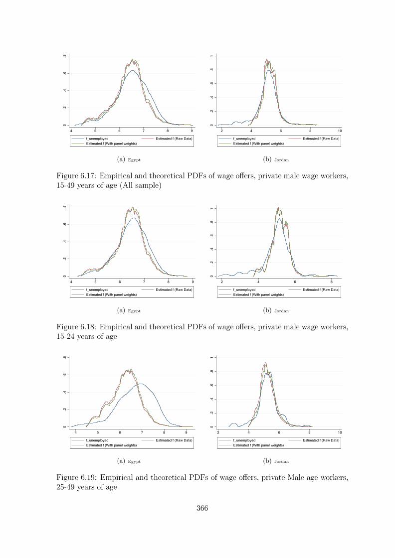
0.2

.4.6

.8

4 5 6 7 8 9

f_unemployed Estimated f (Raw Data)Estimated f (With panel weights)

(a) Egypt

0.2

.4.6

.81

2 4 6 8 10

f_unemployed Estimated f (Raw Data)Estimated f (With panel weights)

(b) Jordan

Figure 6.17: Empirical and theoretical PDFs of wage offers, private male wage workers,15-49 years of age (All sample)

0.2

.4.6

.8

4 5 6 7 8 9

f_unemployed Estimated f (Raw Data)Estimated f (With panel weights)

(a) Egypt

0.2

.4.6

.81

2 4 6 8

f_unemployed Estimated f (Raw Data)Estimated f (With panel weights)

(b) Jordan

Figure 6.18: Empirical and theoretical PDFs of wage offers, private male wage workers,15-24 years of age

0.2

.4.6

.8

4 5 6 7 8 9

f_unemployed Estimated f (Raw Data)Estimated f (With panel weights)

(a) Egypt

0.2

.4.6

.81

2 4 6 8 10

f_unemployed Estimated f (Raw Data)Estimated f (With panel weights)

(b) Jordan

Figure 6.19: Empirical and theoretical PDFs of wage offers, private Male age workers,25-49 years of age

366

General Conclusion

The history of institutions in most developing countries led their labor markets to

be very rigid, where private sector contractual opportunities approached the rules of

public sector appointments. This thesis outsets novel questions about the understand-

ing of labor markets dynamics and the role of insitutions in these developing nations,

particularly Egypt and Jordan. Such markets are generally charcterized by low levels

of employment, high rates of youth unemployment, oversized public sectors and large

unregulated informal sectors. In order to be able to analyze the reasons behing these

stagnant stocks, an exhaustive study of the flows underlying these stocks is needed.

The main objective of this thesis is therefore to look at those specific labor markets,

particularly their labor market flows, under the lens of well-understood and tested

structural models.

Given budgetary and availabilty constraints, it has been shown that panel data,

fielded at relatively spaced dates (points in time), with short retrospective modules to

fill in the gaps between waves are the only best available data one can obtain, short of

continous administrative data, to study the short-term transitions of these labor mar-

kets. These spaced panels can even be absent in some cases, where information can only

be obtained from retrospective questions of a cross-sectional survey. The originality of

the work lies therefore in the extraction of flow dynamics time series of the Egyptian

and Jordanian labor markets from these retrospective accounts. Even with high quality

collection methods and accurate cross-validated questions, these retrospective informa-

tion are however subject to what is referred to as a recall and design bias. Given the

long time interval between, and sometimes the absence of, the waves of the surveys

used, it was not possible to use simple methods of memory bias correction used in pre-

vious literature. A methodological contribution to the literature is therefore provided,

367

where an original method correcting this recall and design error, using the markovian

structure of the labor market transitions, is proposed. Using a Simulated Method of

Moments (SMM), a function representing the ”forgetting rate” conditional on the indi-

vidual’s state in the labor market, is structurally estimated. The correction technique is

very useful in the case of developing countries’ data showing that it is sufficient to have

population, stocks and transitions, moments to correct over- or under-reporting biases

in retrospective data. The correction is done over the different chapters both for the

macro aggregate transitions as well as for the transition and duration individual-level

data. The latter was done by the creation of readily user-friendly micro-data weights.

These could be naive proportional as well as differentiated predicted weights. These

weights, especially the differentiated predicted weights, make significant changes to the

levels and composition of the labor market transitions obtained from the retrospective

data and allows the samples to be corrected and redressed to become random under

the assumptions of the model. The proposed correction methodology assumes a spe-

cific parametric functional form of the estimated error terms. Further work is needed

to expand on the role of this functional form and to test to what extent the obtained

results depend on it. The over-identification of the model can also allow one to develop

tests of fit for the estimated error terms and hence the corrected transition matrices.

Calculating boot-strapped standard errors can also prove very useful in testing for the

significance of the correction methodology and is considered for future work.

The labor market dynamics stylized facts deduced as these flows are constructed and

corrected are the first of this kind and may prove useful to researchers and policy-makers

working on various aspects of the Egyptian and Jordanian labor markets. Knowledge of

those facts is crucial to be able to monitor business cycles, detect inflection points and

assess labor market tightness. It is important to ensure a healthy dynamic labor market

where productive jobs are being created, existing jobs are getting more productive and

less productive jobs are being destroyed. This does not seem to be happening at all

in the Egyptian and Jordanian labor markets where most of the turnover is occurring

in small informal sector jobs, job-to-job transitions are extremely low and when they

occur it is because people are moving within or to the informal sector. One has to

note though that the Jordanian labor market, given the history and evolution of its

368

regulatory institutional framework, is more flexible and mobile than the Egyptian labor

market. Yet, there is some evidence that suggests that the Jordanian labor market is

much more segmented than the Egyptian; the informal sector serving mostly as an

intermediary in Egypt, while in Jordan it appears to be a segment in the market that

functions on its own attracting specific workers. The informality aspect of both markets

surely requires more investigation and further research.

Given the rigidity of these labor markets, major international organizations have

therefore encouraged reforms, to introduce more flexibility in these labor markets. The

second part of the thesis investigates the impact of introducing such flexible employment

protection regulations on the labor market outcomes of these developing countries. In

order to be able to do so, the introduction of the labor law (No.12) in Egypt in 2003 is

evaluated. This Egypt labor law came to action in 2004 aiming at increasing the flexi-

bility of the hiring and firing processes in Egypt. The empirical findings suggest that

the labor market reform increased significantly the separation rates and had no signif-

icant impact on the job finding rates. With increased separations and unchanged job

findings, the unemployment rates in the Egyptian labor market were shifted upwards

after 2004.

These empirical results can be viewed as inconsistent with the usual equilibrium

search Mortensen and Pissarides model, where an increase in the labor market flexi-

bility, modeled as a downward shift of the firing costs, would definitely increase the

separation and the finding rates. Among the possible proposed explanations behind

such an observed unusual phenomenon could be the fact that Egypt is a developing

country where corruption is one of the main barriers to business encountered by the

entrepreneurs. A model is therefore developped to show theoretically how the conven-

tional equilibrium search model can account for this phenomenon and hence to match

the empirical data. In another chapter, this puzzle was also explained by extending

the Mortensen and PIssarides (1994) model to account for the informal and public

sectors, which represent big shares of employment. Even though the policy is directed

to the formal private sector, it surely affects the interaction and the flow of workers

between the different employment sectors. Using the model and numerical analysis, it

was shown that the reform succeeded in scaling down the difference between formal

369

and informal sectors by shifting employment towards the formal sector by liberalizing

it. This has however been accompanied simultaneously by a trending increase in the

real wages of public sector workers and eventually less hiring by government jobs due

to the government’s budegt constraint. Simulating these variations, the model reveals

that the increase in public sector wages tends to crowd out the positive effect on the

private formal sector’s job creation, it even reduces it. The increase in public sector

wages in this case acts as an extra taxation to the job creations in the formal and

informal sector. The net effect observed after the 2004 Egypt labor law is therefore

an increase in the unemployment rates, due to the partial failure of the reform, since

job separations in all cases are enhanced, but job creations remain unchanged or even

dampened.

The developped theoretical model does not limit to explaining the impact of firing

taxes and public sector wages. The aim is to take this work further by testing for

the impact of changes in other policy parameters on the labor market equilibrium and

generalizing the study to other developing labor markets. Another process that has

been neglected in this model and is worth exploring in a future research agenda is

the jobs formalization. Endogenizing productivities and when would jobs be formal or

informal is also an interesting question that can be used to extend the model.

The final part of this thesis investigates the labor market search frictions in the

Egyptian and Jordanian labor market, where these frictions result from the wrokers’

incomplete information about the offered wages. These are important to look through

the quality of jobs accessed by these workers and investigate their movements up the

job ladder. An empirical estimation of a rudimentary partial equilibrium search model

a la Burdett and Mortensen is done, where the Egyptian and Jordanian labor market

surveys are used. The estimated frictional parameters are extremely low confirming

the rigidity of the labor markets in question. The Jordanian labor market proved to

be more flexible than the Egyptian, especially among the younger group of workers.

In Egypt, job offers arrive at a faster rate for the non-employed as they get older,

however in Jordan, it is the reverse. Young Egyptian workers are found to have the

highest level of search frictions, relative to the older Egyptian workers and the Jordanian

workers, implying that the firms’ monopsony power in this trench of the Egyptian

370

market is the highest leading to low levels of salaries. Further work is needed to

re-run estimations of this model, using the differentiated predicted weights. This is

likely to affect the results since the sample limits to private wage workers, who are

likely to mis-report differently than public and non-wage workers for instance. This

also becomes particularly valuable as the distinction between two age groups, who

do not necessarily mis-report the same way, is made. Since the available data allows

the distinction between the different employment sectors, namely public, informal and

formal wage work, it should be interesting to extend the model to include these sectors,

and estimate the frictional parameters as the market is segmented. The comparison

between the simple and extended Burdett-Mortensen frictional parameters might reveal

interesting conclusions relevant to the particular nature of developing countries.

371

Abstract

Policy prescriptions for poor developing countries struggle to expand employment opportunities to

raise their income levels. Among these are the MENA Arab countries that have recently experienced

an unprecedented tide of popular uprisings following the rising poverty, inequality and exclusion, much

of which is related to the labor market. Since the flow approach to labor markets has become the basic

toolbox to modern labor economics, this thesis has at its central insight explaining the functioning of

those specific labor markets, particularly the Egyptian and Jordanian, using the search equilibrium

theory. It looks at analyzing job accession, separations and mobility trends. Overall, evidence of high

levels of rigidity is revealed. The impact of introducing flexible employment protection regulations in

these rigid markets is then discussed both empirically and theoretically. Findings show that lowering

firing costs in Egypt increased significantly the job separations, but had no impact on job creations.

This partial failure of the liberalization reform is interpreted theoretically by a crowding out effect due

to increased corruption set up costs or increased public sector wages. A novel theoretical matching

model a la Mortensen Pissarides is developped allowing for the existence of public, formal private and

informal private sectors, reflecting the particular nature of developing countries. Workers’ movements

up the job ladder is then explored through a structural estimation of the frictional parameters in

a job search model a la Burdett Mortensen. These markets are found to have very high levels of

search frictions especially among the young workers. Given the non-availability of panel data to study

labor market flows, longitudinal retrospective panel datasets are extracted from the Egypt and Jordan

Labor Market Panel Surveys. These panels are then compared to available contemporaneous cross-

sectional information, showing that they suffer from recall and design measurement erros. An original

methodology is therefore proposed and developped to correct the biased labor market transitions

both on the aggregate macro-level, using a Simulated Method of Moments (SMM), as well as on the

micro-individual transaction level, using constructed micro-data weights.

Keywords: Equilibrium search models, recall measurement error, informality, public sector, unem-

ployment, separation, job finding, on-the-job search, Egypt, Jordan.

372

Resume

Dans les pays en voie de developpement, les politiques visent a augmenter les opportunites d’emploi afin

d’elever les revenus et les niveaux de vie des populations. Parmi ces pays, les pays arabes de la region

MENA ont recemment connu une vague de soulevement populaires, faisant suite aux accroissements de

la pauvrete, des inegalites et de l’exclusion, resultats des faibles performances du marche du travail.

Comme l’analyse des flux est devenu l’outil de base de l’economie du travail moderne, cette these

propose d’expliquer le fonctionnement de ces marches du travail assez specifiques, particulierement

ceux de l’Egypte et de la Jordanie, en utilisant la theorie de la recherche d’emploi. Elle se penche sur

l’analyse des creations et destructions d’emploi ainsi que des mobilites entre emplois. Elle montre que

ces marches sont tres rigides. L’impact de l’introduction des reformes structurelles, visant a flexibiliser

l’emploi est ensuite discute de maniere empirique ainsi que theorique. Les resultats montrent que la

baisse des couts de licenciement en Egypte a augmente significativement les destructions d’emploi,

mais n’a eu aucun impact sur les creations. Cet echec partiel de la reforme est un paradoxe empirique,

qui est interprete theoriquement par un effet d’eviction du a l’augmentation du cout de la corruption

ou/et a l’augmentation des salaires du secteur public. Une extension originale du modele theorique de

Mortensen-Pissarides est alors developpe, permettant l’existence de trois secteurs, public, prive formel

et privee informel. Ce cadre rend compte de la nature particuliere des pays en voie de developpement.

Pour examiner la qualite des emplois et pour etudier les avancements dans l’echelle des salaires, une

estimation structurelle du modele de Burdett-Mortensen est ensuite proposee. Elle permet d’etudier

et mesurer les frictions d’appariement sur les marches du travail egyptien et jordanien. Les parametres

estimes sont extremement faibles, soulignant la forte rigidite de ces marches. Le marche du travail

jordanien s’avere, par contre, etre plus flexible que l’egyptien. Compte tenu de la non-disponibilite

de donnees de panels annuelles dans ces pays, il est montre que des donnees de panel retrospectives

peuvent etre utilisees, pour etudier les transitions de court terme sur ces marches du travail. Ces

donnees de panel sont par contre soumises a un biais de memoire. Une methode originale de correction

du biais de memoire est donc proposee et developpee. Elle vise a corriger les transitions a la fois au

niveau macro, en utilisant une methode de moments simules, ainsi qu’au niveau micro, en construisant

des matrices de poids.

Mots-cles: Modeles de recherche d’emploi, biais de rappel, informalite, secteur public, chomage,

creations et destructions d’emploi, mobilite, Egypte, Jordanie.

373