christian gérard - arxiv

Microlocal Analysis of Quantum Fieldson Curved Spacetimes

Christian Gérard

Département de Mathématiques, Université Paris-Saclay, 91405 Or-say Cedex, France

Email address: [email protected]

arX

iv:1

901.

1017

5v2

[m

ath.

AP]

22

Mar

202

1

Contents

Chapter 1. Introduction 11.1. Introduction 11.2. Content 21.3. Notation 4

Chapter 2. Free Klein-Gordon fields on Minkowski spacetime 52.1. Minkowski spacetime 52.2. The Klein-Gordon equation 62.3. Pre-symplectic space of test functions 92.4. The complex case 10

Chapter 3. Fock quantization on Minkowski space 113.1. Bosonic Fock space 113.2. Fock quantization of the Klein-Gordon equation 133.3. Quantum spacetime fields 133.4. Local algebras 14

Chapter 4. CCR algebras and quasi-free states 174.1. Vector spaces 174.2. Bilinear and sesquilinear forms 184.3. Algebras 194.4. States 204.5. CCR algebras 204.6. Quasi-free states 224.7. Covariances of quasi-free states 244.8. The GNS representation of quasi-free states 274.9. Pure quasi-free states 294.10. Examples 33

Chapter 5. Free Klein-Gordon fields on curved spacetimes 355.1. Background 355.2. Lorentzian manifolds 385.3. Stationary and static spacetimes 415.4. Globally hyperbolic spacetimes 425.5. Klein-Gordon equations on Lorentzian manifolds 465.6. Symplectic spaces 48

Chapter 6. Quasi-free states on curved spacetimes 516.1. Quasi-free states on curved spacetimes 516.2. Consequences of unique continuation 536.3. Conformal transformations 54

Chapter 7. Microlocal analysis of Klein-Gordon equations 577.1. Wavefront set of distributions 577.2. Operations on distributions 59

v

vi CONTENTS

7.3. Hörmander’s theorem 617.4. The distinguished parametrices of a Klein-Gordon operator 62

Chapter 8. Hadamard states 658.1. The need for renormalization 658.2. Old definition of Hadamard states 678.3. The microlocal definition of Hadamard states 688.4. The theorems of Radzikowski 698.5. The Feynman inverse associated to a Hadamard state 708.6. Conformal transformations 708.7. Equivalence of the two definitions 708.8. Examples of Hadamard states 728.9. Existence of Hadamard states 72

Chapter 9. Vacuum and thermal states on stationary spacetimes 759.1. Ground states and KMS states 759.2. Klein-Gordon operators 799.3. The Klein-Gordon equation on stationary spacetimes 809.4. Reduction 819.5. Ground and KMS states for P 829.6. Hadamard property 82

Chapter 10. Pseudodifferential calculus on manifolds 8510.1. Pseudodifferential calculus on Rn 8510.2. Pseudodifferential operators on a manifold 8710.3. Riemannian manifolds of bounded geometry 8910.4. The Shubin calculus 9110.5. Time-dependent pseudodifferential operators 9310.6. Seeley’s theorem 9310.7. Egorov’s theorem 93

Chapter 11. Construction of Hadamard states by pseudodifferential calculus 9511.1. Hadamard condition on Cauchy surface covariances 9511.2. Model Klein-Gordon operators 9611.3. Parametrices for the Cauchy problem 9711.4. The pure Hadamard state associated to a microlocal splitting 10111.5. Spacetime covariances and Feynman inverses 10111.6. Klein-Gordon operators on Lorentzian manifolds of bounded

geometry 10211.7. Conformal transformations 10411.8. Hadamard states on general spacetimes 104

Chapter 12. Analytic Hadamard states and Wick rotation 10712.1. Boundary values of holomorphic functions 10712.2. The analytic wavefront set 10912.3. Analytic Hadamard states 11012.4. The Reeh-Schlieder property of analytic Hadamard states 11112.5. Existence of analytic Hadamard states 11212.6. Wick rotation on analytic spacetimes 11212.7. The Calderón projectors 11312.8. The Hadamard state associated to Calderón projectors 11412.9. Examples 115

Chapter 13. Hadamard states and characteristic Cauchy problem 117

CONTENTS vii

13.1. Klein-Gordon fields inside future lightcones 11713.2. The boundary symplectic space 11913.3. The Hadamard condition on the boundary 12013.4. Construction of pure boundary Hadamard states 12213.5. Asymptotically flat spacetimes 12313.6. The canonical symplectic space on I − 126

Chapter 14. Klein-Gordon fields on spacetimes with Killing horizons 12914.1. Spacetimes with bifurcate Killing horizons 13014.2. Klein-Gordon fields 13114.3. Wick rotation 13114.4. The double β-KMS state inM+ ∪M− 13314.5. The extended Euclidean metric and the Hawking temperature 13414.6. The Hartle-Hawking-Israel state 134

Chapter 15. Hadamard states and scattering theory 13715.1. Klein-Gordon operators on asymptotically static spacetimes 13715.2. The in and out vacuum states 13815.3. Reduction to a model case 140

Chapter 16. Feynman propagator on asymptotically Minkowski spacetimes 14316.1. Klein-Gordon operators on asymptotically Minkowski spacetimes 14416.2. The Feynman inverse of P 14416.3. Construction of the Feynman inverse 145

Chapter 17. Dirac fields on curved spacetimes 15117.1. CAR ∗-algebras and quasi-free states 15117.2. Clifford algebras 15217.3. Clifford representations 15317.4. Spin groups 15417.5. Weyl bi-spinors 15517.6. Clifford and spinor bundles 15617.7. Spin structures 15817.8. Spinor connections 15817.9. Dirac operators 15917.10. Dirac equation on globally hyperbolic spacetimes 16017.11. Quantization of the Dirac equation 16217.12. Hadamard states for the Dirac equation 16217.13. Conformal transformations 16317.14. The Weyl equation 16417.15. Relationship between Dirac and Weyl Hadamard states 166

Bibliography 167

CHAPTER 1

Introduction

1.1. Introduction

Quantum Field Theory arose from the need to unify Quantum Mechanics withspecial relativity. It is usually formulated on the flat Minkowski spacetime, on whichclassical field equations, such as the Klein-Gordon, Dirac or Maxwell equations areeasily defined. Their quantization rests on the so-called Minkowski vacuum, whichdescribes a state of the quantum field containing no particles. The Minkowskivacuum is also fundamental for the perturbative or non-perturbative constructionof interacting theories, corresponding to the quantization of non-linear classical fieldequations.

Quantum Field Theory on Minkowski spacetime relies heavily on its symmetryunder the Poincaré group. This is apparent in the ubiquitous role of plane waves inthe analysis of classical field equations, but more importantly in the characterizationof the Minkowski vacuum as the unique state which is invariant under the Poincarégroup and has some energy positivity property.

Quantum Field Theory on curved spacetimes describes quantum fields in anexternal gravitational field, represented by the Lorentzian metric of the ambientspacetime. It is used in situations when both the quantum nature of the fields andthe effect of gravitation are important, but the quantum nature of gravity can beneglected in a first approximation. Its non-relativistic analog would be for exampleordinary Quantum Mechanics, i.e. the Schrödinger equation, in a classical exteriorelectromagnetic field.

Its most important areas of application are the study of phenomena occurringin the early universe and in the vicinity of black holes, and its most celebrated resultis the discovery by Hawking that quantum particles are created near the horizon ofa black hole.

The symmetries of the Minkowski spacetime, which play such a fundamentalrole, are absent in curved spacetimes, except in some simple situations, like sta-tionary or static spacetimes. Therefore, the traditional approach to quantum fieldtheory has to be modified: one has first to perform an algebraic quantization, whichfor free theories amounts to introducing an appropriate phase space, which is ei-ther a symplectic or an Euclidean space, in the bosonic or fermionic case. Fromsuch a phase space one can construct CCR or CAR ∗-algebras, and actually nets of∗-algebras, each associated to a region of spacetime.

The second step consists in singling out, among the many states on these ∗-algebras, the physically meaningful ones, which should resemble the Minkowskivacuum, at least in the vicinity of any point of the spacetime. This leads to thenotion of Hadamard states, which were originally defined by requiring that theirtwo-point functions have a specific asymptotic expansion near the diagonal, calledthe Hadamard expansion.

A very important progress was made by Radzikowski, [R1, R2], who intro-duced the characterization of Hadamard states by the wavefront set of their two-point functions. The wavefront set of a distribution is the natural way to describe

1

2 1. INTRODUCTION

its singularities in the cotangent space, and lies at the basis of microlocal analysis,a fundamental tool in the analysis of linear and non-linear partial differential equa-tions. Among its avatars in the physics literature are, for example, the geometricaloptics in wave propagation and the semi-classical limit in Quantum Mechanics.

The introduction of microlocal analysis in quantum field theory on curvedspacetimes started a period of rapid progress, non only for free (i.e. linear) quantumfields, but also for the perturbative construction of interacting fields by Brunettiand Fredenhagen [BF]. For free fields it allowed to use several fundamental resultsof microlocal analysis, like Hörmander’s propagation of singularities theorem andthe classification of parametrices for Klein-Gordon operators by Duistermaat andHörmander.

1.2. Content

The goal of these lecture notes is to give an exposition of microlocal analysismethods in the study of Quantum Field Theory on curved spacetimes. We willfocus on free fields and the corresponding quasi-free states and more precisely onKlein-Gordon fields, obtained by quantization of linear Klein-Gordon equations onLorentzian manifolds, although the case of Dirac fields will be described in Chapter17.

There exist already several good textbooks or lecture notes on quantum fieldtheory in curved spacetimes. Among them let us mention the book by Bär, Ginouxand Pfaeffle [BGP], the lecture notes [BFr] and [BDFY], the more recent bookby Rejzner [Re], and the survey by Benini, Dappiagi and Hack [BDH]. Thereexist also more physics oriented books, like the books by Wald [W2], Fulling [F]and Birrell and Davies [BD]. Several of these texts contain important developmentswhich are not described here, like the perturbative approach to interacting theories,or the use of category theory.

In this lecture notes we focus on advanced methods from microlocal analysis,like for example pseudodifferential calculus, which turn out to be very useful in thestudy and construction of Hadamard states.

Pure mathematicians working in partial differential equations are often deterredby the traditional formalism of quantum field theory found in physics textbooks,and by the fact that the construction of interacting theories is, at least for the timebeing, restricted to perturbative methods.

We hope that these lecture notes will convince them that quantum field theoryon curved spacetimes is full of interesting and physically important problems, witha nice interplay between algebraic methods, Lorentzian geometry and microlocalmethods in partial differential equations. On the other hand, mathematical physi-cists with a traditional education, which may lack familiarity with more advancedtools of microlocal analysis, can use this text as an introduction and motivation tothe use of these methods.

Let us now give a more detailed description of these lecture notes. The readermay also consult the introduction of each chapter for more information.

For pedagogical reasons, we have chosen to devote Chapters 2 and 3 to abrief outline of the traditional approach to quantization of Klein-Gordon fieldson Minkowski spacetime, but the impatient reader can skip them without trouble.

Chapter 4 deals with CCR ∗-algebras and quasi-free states. A reader with aPDE background may find the reading of this chapter a bit tedious. Nevertheless,we think it is worth the effort to get familiar with the notions introduced there.

In Chapter 5 we describe well-known concepts and results concerning Lorentzianmanifolds and Klein-Gordon equations on them. The most important are the notion

1.2. CONTENT 3

of global hyperbolicity, a property of a Lorentzian manifold implying global solvabil-ity of the Cauchy problem, and the causal propagator and the various symplecticspaces associated to it.

In Chapter 6 we discuss quasi-free states for Klein-Gordon fields on curvedspacetimes, which is a concrete application of the abstract formalism in Chapter 4.Of interest are the two possible descriptions of a quasi-free state, either by it space-time covariances, or by its Cauchy surface covariances, which are both importantin practice. Another useful point is the discussion of conformal transformations.

Chapter 7 is devoted to the microlocal analysis of Klein-Gordon equations. Wecollect here various well-known results about wavefront sets, Hörmander’s propaga-tion of singularities theorem and its related study with Duistermaat of distinguishedparametrices for Klein-Gordon operators, which play a fundamental role in quan-tized Klein-Gordon fields.

In Chapter 8 we introduce the modern definition of Hadamard states due toRadzikowski and discuss some of its consequences. We explain the equivalence withthe older definition based on Hadamard expansions and the well-known existenceresult by Fulling, Narcowich and Wald.

In Chapter 9 we discuss ground states and thermal states, first in an abstractsetting, then for Klein-Gordon operators on stationary spacetimes. Ground statesshare the symmetries of the background stationary spacetime and are the naturalanalogs of the Minkowski vacuum. In particular, they are the simplest examples ofHadamard states.

Chapter 10 is devoted to an exposition of a global pseudodifferential calculus onnon compact manifolds, the Shubin calculus. This calculus is based on the notionof manifolds of bounded geometry and is a natural generalization of the standarduniform calculus on Rn. Its most important properties are the Seeley and Egorovtheorems.

In Chapter 11 we explain the construction of Hadamard states using the pseu-dodifferential calculus in Chapter 10. The construction is done, after choosing aCauchy surface, by a microlocal splitting of the space of Cauchy data obtained froma global construction of parametrices for the Cauchy problem. It can be appliedto many spacetimes of physical interest, like the Kerr-Kruskal and Kerr-de Sitterspacetimes.

In Chapter 12 we construct analytic Hadamard states by Wick rotation, a well-known procedure in Minkowski spacetime. Analytic Hadamard states are definedon analytic spacetimes, by replacing the usual C∞ wavefront set by the analyticwavefront set, which describes the analytic singularities of distributions. Like theMinkowski vacuum, they have the important Reeh-Schlieder property. After Wickrotation, the hyperbolic Klein-Gordon operator becomes an elliptic Laplace oper-ator, and analytic Hadamard states are constructed using a well-known tool fromelliptic boundary value problems, namely the Calderón projector.

In Chapter 13 we describe the construction of Hadamard states by the charac-teristic Cauchy problem. This amounts to replacing the space-like Cauchy surfacein Chapter 11 by a past or future lightcone, choosing its interior as the ambientspacetime. From the trace of solutions on this cone one can introduce a boundarysymplectic space, and it turns out that it is quite easy to characterize states onthis symplectic space which generate a Hadamard state in the interior. Its mainapplication is the conformal wave equation on spacetimes which are asymptoticallyflat at past or future null infinity. We also describe in this chapter the BMS groupof asymptotic symmetries of these spacetimes, and its relationship with Hadamardstates.

4 1. INTRODUCTION

In Chapter 14 we discuss Klein-Gordon fields on spacetimes with Killing hori-zons. Our aim is to explain a phenomenon loosely related with the Hawking ra-diation, namely the existence of the Hartle-Hawking-Israel vacuum, on spacetimeshaving a stationary Killing horizon. The construction and properties of this statefollow from the Wick rotation method already used in Chapter 12, the Calderónprojectors playing also an important role.

Chapter 15 is devoted to the construction of Hadamard states by scatteringtheory methods. We consider spacetimes which are asymptotically static at past orfuture time infinity. In this case one can define the in and out vacuum states, whichare states asymptotic to the vacuum state at past or future time infinity. Using thetools from Chapters 10, 11 we prove that these states are Hadamard states.

In Chapter 16 we discuss the notion of Feynman inverses. It is known that aKlein-Gordon operator on a globally hyperbolic spacetime admits Feynman para-metrices, which are unique modulo smoothing operators and characterized by thewavefront set of its distributional kernels. One can ask if one can also define aunique, canonical true inverse, having the correct wavefront set. We give a positiveanswer to this question on spacetimes which are asymptotically Minkowski.

Chapter 17 is devoted to the quantization of the Dirac equation and to thedefinition of Hadamard states for Dirac quantum fields. The Dirac equation ona curved spacetime describes an electron-positron field which is a fermionic field,and the CCR ∗-algebra for the Klein-Gordon field has to be replaced by a CAR∗-algebra. Apart from this difference, the theory for fermionic fields is quite parallelto the bosonic case. We also describe the quantization of the Weyl equation, whichoriginally was thought to describe massless neutrinos.

1.2.1. Acknowledgments. The results described in Chapters 11, 12, 15, andpart of those in Chapters 10 and 13, originate from common work with MichalWrochna, over a period of several years.

I learned a lot of what I know about quantum field theory from my long collab-oration with Jan Derezinski, and several parts of these lecture notes, like Chapters4 and 5 borrow a lot from our common book [DG]. I take the occasion here toexpress my gratitude to him.

Finally, I also greatly profited from discussions with members of the AQFTcommunity. Among them I would like to especially thank Claudio Dappiagi, ValterMoretti, Nicola Pinamonti, Igor Khavkine, Klaus Fredenhagen, Detlev Bucholz,Wojciech Dybalski, Kasia Rejzner, Dorothea Bahns, Rainer Verch, Stefan Hollandsand Ko Sanders.

1.3. Notation

We now collect some notation that we will use.We set 〈λ〉 = (1 + λ2)

12 for λ ∈ R.

We write A b B if A is relatively compact in B.If X,Y are sets and f : X → Y we write f : X

∼−→ Y if f is bijective. If X,Yare equipped with topologies, we write f : X → Y if the map is continuous, andf : X

∼−→ Y if it is a homeomorphism.

1.3.1. Scale of abstract Sobolev spaces. Let H a real or complex Hilbertspace and A a selfadjoint operator on H. We write A > 0 if A ≥ 0 and KerA = 0.

If A > 0 and s ∈ R, we equip DomA−s with the scalar product (u|v)−s =(A−su|A−sv) and the norm ‖A−su‖. We denote by AsH the completion of DomA−s

for this norm, which is a (real or complex) Hilbert space.

CHAPTER 2

Free Klein-Gordon fields on Minkowski spacetime

Almost all textbooks on quantum field theory start with the quantization ofthe free (i.e. linear) Klein-Gordon and Dirac equations on Minkowski spacetime.The traditional exposition rests on the so-called frequency splitting, which amountsto splitting the space of solutions of, say, the Klein-Gordon equation into two sub-spaces, corresponding to solutions having positive/negative energy, or equivalentlywhose Fourier transforms are supported in the upper/lower mass hyperboloid.

One then proceeds with the introduction of Fock spaces and the definition ofquantized Klein-Gordon or Dirac fields using creation/annihilation operators.

Since it relies on the use of the Fourier transformation, this method does notcarry over to Klein-Gordon fields on curved spacetimes. More fundamentally, it hasthe drawback of mixing two different steps in the quantization of the Klein-Gordonequation.

The first, purely algebraic step consists in using the symplectic nature of theKlein-Gordon equation to introduce an appropriate CCR ∗-algebra. The secondstep consists in choosing a state on this algebra, which on the Minkowski spacetimeis the vacuum state.

Nevertheless it is useful to keep in mind the Minkowski spacetime as an impor-tant example. This chapter is devoted to the classical theory of the Klein-Gordonequation on Minkowski spacetime, i.e. to its symplectic structure. Its Fock quan-tization will be described in Chapter 3.

2.1. Minkowski spacetime

In the sequel we will use notation introduced later in Section 4.1.The elements of Rn = Rt × Rdx will be denoted by x = (t, x), those of the dual

(Rn)′ by ξ = (τ, k).

2.1.1. The Minkowski spacetime.

Definition 2.1.1. The Minkowski spacetime R1,d is R1+d equipped with thebilinear form η ∈ Ls(R1+d, (R1+d)′) given by

(2.1) x·ηx = −t2 + x2.

Definition 2.1.2. (1) A vector x ∈ R1,d is time-like if x ·ηx < 0, null ifx·ηx = 0, causal if x·ηx ≤ 0, and space-like if x·ηx > 0.

(2) C± ··= x ∈ R1,d : x ·ηx < 0, ±t > 0, resp. C± ··= x ∈ R1,d : x ·ηx ≤0, ±t ≥ 0 are called the open, resp. closed future/past (solid) lightcones.

(3) N ··= x ∈ R1,d : x · ηx = 0, resp. N± = N ∩ ±t ≥ 0 are called the nullcone resp. future/past null cones.

There is a similar classification of vector subspaces of R1,d.

Definition 2.1.3. A linear subspace V of R1,d is time-like if it contains bothspace-like and time-like vectors, null if it is tangent to the null cone N and space-likeif it contains only space-like vectors.

5

6 2. FREE KLEIN-GORDON FIELDS ON MINKOWSKI SPACETIME

Definition 2.1.4. (1) If K ⊂ R1,d, I±(K) ··= K + C±, resp. J±(K) ··=K + C±, is called the time-like, resp. causal future/past of K, and J(K) ··=J+(K) ∪ J−(K) the causal shadow of K.

(2) Two sets K1, K2 are called causally disjoint if K1∩J(K2) = ∅ or, equivalently,if J(K1) ∩K2 = ∅.

(3) A function f on Rn is called space-compact, resp. future/past space-compact,if supp f ⊂ J(K), resp. supp f ⊂ J±(K) for some compact set K b Rn. Thespaces of smooth such functions will be denoted by C∞sc (Rn), resp. C∞sc,±(Rn).

2.1.2. The Lorentz and Poincaré groups.

Definition 2.1.5. (1) The pseudo-Euclidean group O(R1+d, η) is denoted byO(1, d) and is called the Lorentz group.

(2) SO(1, d) is the subgroup of L ∈ O(1, d) with detL = 1.(3) If L ∈ O(1, d) one has L(J+) = J+ or L(J+) = J−. In the first case L is

called orthochronous and in the second anti-orthochronous.(4) The subgroup of orthochronous elements of SO(1, d) is denoted by SO↑(1, d)

and called the restricted Lorentz group.

Definition 2.1.6. The (restricted) Poincaré group is the set P (1, d) ··= Rn ×SO↑(1, d) equipped with the product

(a2, L2)× (a1, L1) = (a2 + L2a1, L2L1).

The Poincaré group acts on Rn by Λx ··= Lx+ a for Λ = (a, L) ∈ P (1, d).

2.2. The Klein-Gordon equation

We recall that the differential operator

P = −2 +m2 ··= ∂2t −

d∑i=1

∂2xi +m2,

for m ≥ 0 is called the Klein-Gordon operator.We set ε(k) = (k2 + m2)

12 and denote by ε = ε(Dx) the Fourier multiplier

defined by F(εu)(k) = ε(k)u(k), where Fu(k) = (2π)−d/2´

e−ik·xu(x)dx is the(unitary) Fourier transform. Note that −2 +m2 = ∂2

t + ε2.The Klein-Gordon equation

(2.2) −2φ+m2φ = 0

is the simplest relativistic field equation. Its quantization describes a scalar bosonicfield of massm. The wave equation (m = 0) is a particular case of the Klein-Gordonequation. Note that since −2 + m2 preserves real functions, the Klein-Gordonequation has real solutions, which are associated to neutral fields, correspondingto neutral particles, while the complex solutions are associated to charged fields,corresponding to charged particles.

It will be more convenient later to consider complex solutions, but in thischapter we will, as is usual in the physics literature, consider mainly real solutions.The case of complex solutions will be briefly discussed in Section 2.4.

We refer the reader to Chapter 4 for a general discussion of the real vs complexformalism in a more abstract framework.

We are interested in the space of its smooth, space-compact, real solutions de-noted by Solsc,R(KG). Solsc,R(KG) is invariant under the Poincaré group if weset

(2.3) αΛφ(x) ··= φ(Λ−1x), Λ ∈ P (1, d).

2.2. THE KLEIN-GORDON EQUATION 7

2.2.1. The Cauchy problem. If φ ∈ C∞(Rn) and t ∈ R we set φ(t)(x) ··=φ(t, x) ∈ C∞(Rd). Any solution φ ∈ Solsc,R(KG) is determined by its Cauchy dataon the Cauchy surface Σs = t = s ∼ Rd, defined by the map

(2.4) %sφ ··=(

φ(s)∂tφ(s)

)= f ∈ C∞0 (Rd;R2).

The unique solution in Solsc,R(KG) of the Cauchy problem

(2.5)

(−2 +m2)φ = 0,%sφ = f,

is denoted by φ = Usf and given by

(2.6) φ(t) = cos(ε(t− s))f0 + ε−1 sin(ε(t− s)f1, f =

(f0

f1

).

The map Us is called the Cauchy evolution operator. The following propositionexpresses the important causality property of Us.

Proposition 2.2.1. One has

suppUsf ⊂ J(s × supp f).

2.2.2. Advanced and retarded inverses. Let us now consider the inhomo-geneous Klein-Gordon equation

(2.7) (−2 +m2)u = v,

where for simplicity v ∈ C∞0 (Rn). Since there are plenty of homogeneous solutions,it is necessary to supplement (2.7) by support conditions to obtain unique solutions,by requiring that φ vanishes for large negative or positive times.

Theorem 2.2.2. (1) there exist unique solutions uret/adv = Gret/advv ∈ C∞±sc (Rn)of (2.7). Setting

(2.8) Gret/adv(t) ··= ±θ(±t)ε−1 sin(εt),

where θ(t) = 1l[0,+∞[(t) is the Heaviside function, one has

(2.9) Gret/advv(t, ·) =

ˆRGret/adv(t− s)v(s, ·)ds;

(2) one has suppGret/advv ⊂ J±(supp v).

The operators Gret/adv are called the retarded/advanced inverses of P . Let usequip C∞0 (Rn) with the scalar product

(2.10) (u|v)Rn ··=ˆRnuvdx,

and C∞0 (Rd;C2) with the scalar product

(2.11) (f |g)Rd =

ˆRd

(f1g1 + f0g0

)dx.

It follows from (2.8) thatG∗ret/adv = Gadv/ret,

where A∗ denotes the formal adjoint of A with respect to the scalar product (·|·)Rn .The operator

(2.12) G ··= Gret −Gadv

is called in the physics literature the Pauli-Jordan or commutator function, or alsothe causal propagator. Note that

(2.13) G = −G∗, suppGv ⊂ J(supp v),


and

(2.14) Gv(t, ·) =

ˆRε−1 sin(ε(t− s))v(s, ·)ds.

There is an important relationship between G and Us. Namely, if we denote by%∗s : D′(Rd;R2) → D′(Rn) the formal adjoint of %s : C∞0 (Rn) → C∞0 (Rd;R2) withrespect to the scalar products (2.10) and (2.11), then:

(2.15) %∗sf(t, x) = δs(t)⊗ f0(x)− δ′s(t)⊗ f1(x), f ∈ C∞(Rd;R2).

The following lemma follows from (2.6), (2.8) by a direct computation.

Lemma 2.2.3. One has

Usf = G∗ %∗s σf, f ∈ C∞0 (Rd;R2),

for σ =

(0 −1l1l 0

).

2.2.3. Symplectic structure. It is well-known that the Klein-Gordon equa-tion is a Hamiltonian equation. Indeed let us equip C∞0 (Rd;R2) with the symplecticform:

(2.16) f ·σg ··=ˆRd

(f1g0 − f0g1

)dx.

If we identify bilinear forms on C∞0 (Rd;R2) with linear operators using the scalarproduct (·|·)Rd , we have

f ·σg = (f |σg)Rd ,

where the operator σ is defined in Lemma 2.2.3. If we introduce the classicalHamiltonian

f ·Ef ··=1

2

ˆRd

(f2

1 + f0ε2f0

)dx

and define A ∈ L(C∞0 (Rd;R2)) by

(2.17) f ·σAg ··= f ·Eg, f, g ∈ C∞0 (Rd;R2),

we obtain that

A =

(0 1l−ε2 0

).

Setting f(t) = %tU0f for f ∈ C∞0 (Rd;C2) we have, by an easy computation

(2.18) f(t) = etAf,

which shows that f 7→ f(t) is the symplectic flow generated by the classical Hamil-tonian E and the symplectic form σ. In particular, if fi(t) = etAfi, i = 1, 2,f1(t)·σf2(t) is independent on t.

Equivalently, we can equip Solsc,R(KG) with the symplectic form

(2.19) φ1 ·σφ2 ··= %tφ1 ·σ%tφ2,

where the right-hand side is independent on t. Fixing the reference Cauchy surfaceΣ0 ∼ Rd, we obtain the following proposition:

Proposition 2.2.4. The Cauchy data map on Σ0

%0 : (Solsc,R(KG), σ) −→ (C∞0 (Rd;R2), σ),

is symplectic, with %−10 = U0, where the Cauchy evolution operator Us was intro-

duced in Subsection 2.2.1.

2.3. PRE-SYMPLECTIC SPACE OF TEST FUNCTIONS 9

This leads to another interpretation of (2.18): the space Solsc,R(KG) is invari-ant under the group of time translations

τsφ(·, x) ··= φ(· − s, x),

and τs is symplectic on (Solsc,R(KG), σ). Then (2.18) can be rewritten as

%0 τs %−10 = esA, s ∈ R.

2.3. Pre-symplectic space of test functions

By Proposition 2.2.4, (Solsc,R(KG), σ) is a symplectic space. It is easy to seethat αΛ defined in (2.3) is symplectic if Λ is orthochronous, for example using The-orem 2.3.2 below. If Λ is anti-orthochronous, αΛ is anti-symplectic, i.e. transformsσ into −σ.

Identifying (Solsc,R(KG), σ) with (C∞0 (Rd;R2), σ) using %0 is convenient forconcrete computations, but destroys Poincaré invariance, since one fixes the Cauchysurface Σ0. It would be useful to have another isomorphic symplectic space whichis Poincaré invariant and at the same time easier to understand than Solsc,R(KG).It turns out that one can use the space of test functions C∞0 (Rn;R), which is afundamental step in formulating the notion of locality for quantum fields.

Proposition 2.3.1. Consider the map G : C∞0 (Rn;R)→ C∞sc (Rn). Then:

(1) RanG = Solsc,R(KG),

(2) KerG = PC∞0 (Rn;R).

Moreover, we have(3) (%0G)∗ σ (%0G) = G.

Proof. (1) By P G = 0 and Theorem 2.2.2 (2), we see that RanG ⊂ Solsc,R(KG).Conversely let φ ∈ Solsc,R(KG). If fs = %sφ, then by Lemma 2.2.3 we obtain thatφ = −G %∗s σfs for s ∈ R. Hence, if χ ∈ C∞0 (R) with

´χ(s)ds = 1 we obtain

thatφ =

ˆRχ(s)φds = Gv,

for v = −´R χ(s)%∗s σfsds ∈ C∞0 (Rn).

(2) Since G P = 0 we have PC∞0 (Rn;R) ⊂ KerG. Conversely let v ∈C∞0 (Rn;R) with Gv = 0. Then for uret/adv = Gret/advv we have uret = uadv =·· u,u ∈ C∞0 (Rn) by Theorem 2.2.2 (2) and v = Pu since P Gret/adv = 1l.

(3) We have, using (2.14)

%0Gu =

(−´ε−1 sin(εs)u(s)ds´cos(εs)u(s)ds

),

hence

σ (%0G)u = −( ´

cos(εs)u(s)ds´ε−1 sin(εs)u(s)ds

),

and(%0G)∗f = −G%∗0f

= −´ε−1 sin(ε(t− s))(δ0(s)⊗ f0 − δ′0(s)⊗ f1)ds

= −ε−1 sin(εt)f0 + cos(εt)f1,

which yields

(%0G)∗ σ (%0G)u

=´ε−1 sin(εt) cos(εs)u(s)ds+

´ε−1 cos(εt) sin(εs)u(s)ds

=´ε−1 sin(ε(t− s))u(s)ds = Gu.


This completes the proof of the proposition. 2

One can summarize Propositions 2.2.4 and 2.3.1 in the following theorem:

Theorem 2.3.2. (1) The following spaces are symplectic spaces:

(C∞0 (Rn;R)

PC∞0 (Rn;R), (·|G·)Rn), (Solsc,R(KG), σ), (C∞0 (Rd;R2), σ).

(2) The following maps are symplectomorphisms:

(C∞0 (Rn;R)

PC∞0 (Rn;R), (·|G·)Rn)

G−→(Solsc,R(KG), σ)%0−→(C∞0 (Rd;R2), σ).

The first and last of these equivalent symplectic spaces are the most useful forthe quantization of the Klein-Gordon equation.

2.4. The complex case

Let us now discuss the space Solsc,C(KG) of complex space-compact solutions.We refer to Section 4.2 for notation and terminology.

It is more natural to use the map

(2.20) %sφ ··=(

φ(s)i−1∂tφ(s)

)as Cauchy data map and to equip the space C∞0 (Rd;C2) of Cauchy data with theHermitian form

(2.21) f ·qg ··=ˆRd

(f1g0 + f0g1

)dx.

The space Solsc,C(KG) is similarly equipped with the form

φ1 ·qφ2 ··= %tφ1 ·q%tφ2,

which is independent on t. The Cauchy evolution operator becomes

(2.22) U0f(t) = cos(εt)f0 + iε−1 sin(εt)f1.

We have then the following analog of Theorem 2.3.2:

Theorem 2.4.1. (1) The following spaces are Hermitian spaces:

(C∞0 (Rn;C)

PC∞0 (Rn;C), (·|iG·)Rn), (Solsc,C(KG), q), (C∞0 (Rd;C2), q).

(2) The following maps are unitary:

(C∞0 (Rn;C)

PC∞0 (Rn;C), (·|iG·)Rn)

G−→(Solsc,C(KG), q)%0−→(C∞0 (Rd;C2), q).

CHAPTER 3

Fock quantization on Minkowski space

We describe in this chapter the Fock quantization of the Klein-Gordon equationon Minkowski spacetime. We recall the definition of the bosonic Fock space over aone-particle space and of the creation/annihilation operators, which are ubiquitousnotions in quantum field theory.

For example, it is common in the physics oriented literature to specify a statefor the Klein-Gordon field by defining first some creation/annihilation operators.We will see in Chapter 4 that this is nothing else than choosing a particular Kählerstructure on a certain symplectic space.

In this approach the quantum Klein-Gordon fields are defined as linear oper-ators on the Fock space, so one has to pay attention to domain questions. Thesetechnical problems disappear if one uses a more abstract point of view and intro-duces the appropriate CCR ∗-algebra, as will be done in Chapter 4. Fock spaceswill reappear as the (Gelfand-Naimark-Segal) GNS Hilbert spaces associated to apure quasi-free state on this algebra. Apart from this fact, they can be forgotten.

3.1. Bosonic Fock space

3.1.1. Bosonic Fock space. Let h be a complex Hilbert space whose unitvectors describe the states of a quantum particle. If this particle is bosonic, then thestates of a system of n such particles are described by unit vectors in the symmetrictensor power ⊗ns h, where we take the tensor products in the Hilbert space sense,i.e. complete the algebraic tensor products for the natural Hilbert norm.

A system of an arbitrary number of particles is described by the bosonic Fockspace

(3.1) Γs(h) ··=∞⊕n=0

⊗ns h,

where the direct sum is again taken in the Hilbert space sense and ⊗0sh = C by

definition. We recall that the symmetrized tensor product is defined by

Ψ1 ⊗s Ψ2 ··= Θs(Ψ1 ⊗Ψ2),

whereΘs(u1 ⊗ · · · ⊗ un) =

1

n!

∑σ∈Sn

uσ(1) ⊗ · · · ⊗ uσ(n).

The vector Ωvac = (1, 0, . . . ) is called the vacuum and describe a state with noparticles at all. A useful observable on Γs(h) is the number operator N , whichcounts the number of particles, defined by

N |⊗ns h = n1l.

The operator N is an example of a second quantized operator, namely N = dΓ(1l),where

dΓ(a)|⊗ns h ··=n∑j=1

1l⊗j−1 ⊗ a⊗ 1l⊗n−j ,

11

12 3. FOCK QUANTIZATION ON MINKOWSKI SPACE

for a a linear operator on h.

3.1.2. Creation/annihilation operators. Since Γs(h) describes an arbitrarynumber of particles, it is useful to have operators that create or annihilate particles.One defines the creation/annihilation operators by

a∗(h)Ψn ··=√n+ 1h⊗s Ψn,

a(h)Ψn ··=√n(h| ⊗ 1l⊗n−1Ψn, Ψn ∈ ⊗ns (h), h ∈ h,

where one sets (h|u = (h|u) for u ∈ h. It is easy to see that a(∗)(h) are well definedon DomN

12 and that (Ψ1|a∗(h)Ψ2) = (a(h)Ψ1|Ψ2), i.e. a(h)∗ ⊂ a∗(h) on DomN

12 .

Moreover

(3.2) h 3 h 7→ a∗(h), resp. a(h) is C-linear, resp. anti-linear,

and as quadratic forms on DomN12 one has

(3.3)[a(h1), a(h2)] = [a∗(h1), a∗(h2)] = 0,

[a(h1), a∗(h2)] = (h1|h2)1l, h1, h2 ∈ h,

where [A,B] = AB −BA, which a version of the canonical commutation relations,abbreviated CCR in the sequel.

3.1.3. Field and Weyl operators. One then introduces the field operatorsin the Fock representation

(3.4) φF(h) ··=1√2

(a(h) + a∗(h)), h ∈ h,

which can be easily shown to be essentially selfadjoint on DomN12 . One has

(3.5) φF(h1 + λh2) = φF(h1) + λφF(h2), λ ∈ R, hi ∈ h, on DomN12 ,

i.e. h 7−→ φF(h) is R-linear, and the Heisenberg form of the CCR are satisfied asquadratic forms on DomN

12

(3.6) [φF(h1), φF(h2)] = ih1 ·σh21l.

for

(3.7) h1 ·σh2 = Im(h1|h2).

Denoting again by φF(h) the selfadjoint closure of φF(h), one can then define theWeyl operators

(3.8) WF(h) ··= eiφF(h),

which are unitary and satisfy the Weyl form of the CCR

WF(h1)WF(h2) = e−ih1·σh2WF(h1 + h2).

If hR denotes the real form of h, i.e. h as a real vector space, then (hR, σ) is areal symplectic space. Moreover i, considered as an element of L(hR), belongs toSp(hR, σ) and one has

ν ··= σ i = Re(·|·) ≥ 0.

3.3. QUANTUM SPACETIME FIELDS 13

3.1.4. Kähler structures. In general, a triple (X , σ, j), where (X , σ) is a realsymplectic space and j ∈ L(X ) satisfies j2 = −1l and σ j ∈ Ls(X ,X ′), is calleda pseudo-Kähler structure on X . If σ j ≥ 0, it is called a Kähler structure. Theanti-involution j is called a Kähler anti-involution. We will come back to this notionin Section 4.1. Given a Kähler structure on X , one can turn X into a complex pre-Hilbert space by equipping it with the complex structure j and the scalar product:

(3.9) (x1|x2)F ··= x1 ·σjx2 + ix1 ·σx2.

If we choose as one-particle Hilbert space the completion of X for (·|·)F, we canconstruct the Fock representation by the map

X 3 x 7−→ φF(x)

which satisfies (3.5), (3.6).

3.2. Fock quantization of the Klein-Gordon equation

From the above discussion we see that the first step in the construction of quan-tum Klein-Gordon fields is to fix a Kähler anti-involution on one of the equivalentsymplectic spaces in Theorem 2.3.2, the most convenient one being (C∞0 (Rd;R2), σ).

3.2.1. The Kähler structure. There are plenty of choices of Kähler anti-involutions. The most natural one is obtained as follows: let us denote by h thecompletion of C∞0 (Rd;C) with respect to the scalar product

(h1|h2)F ··= (h1|ε−1h2)Rd .

If m > 0, this space is the (complex) Sobolev space H−12 (Rd) and if m = 0 the

complex homogeneous Sobolev space H−12 (Rd), except when d = 1, since the in-

tegral´R |k|

−1dk diverges at k = 0. This is an example of the so-called infraredproblem for massless fields in two spacetime dimensions.

To avoid a somewhat lengthy digression, we will assume that m > 0 if d = 1.Let us introduce the map

(3.10) V : C∞0 (Rd;R2) 3 f 7−→ εf0 − if1 ∈ h.

An easy computation shows that:

Im(V f |V g)F = f ·σg,

i V =·· V j, for j =

(0 ε−1

−ε 0

),

eitε V = V etA.

In other words, j is a Kähler anti-involution on C∞0 (Rd;R2) and the associated one-particle Hilbert space is unitarily equivalent to h. Moreover, after identification byV , the symplectic group etAt∈R becomes the unitary group eitεt∈R with positivegenerator ε. This positivity is the distinctive feature of the Fock representation.

3.3. Quantum spacetime fields

Let us set

(3.11) ΦF(u) =

ˆRφF(e−itεu(t, ·))dt, u ∈ C∞0 (Rn;R),

the integral being for example norm convergent in B(DomN12 ,Γs(h)). We obtain

from (2.14) and (3.7) that

(3.12) [ΦF(u),ΦF(v)] = i(u|Gv)Rn1l,

14 3. FOCK QUANTIZATION ON MINKOWSKI SPACE

and ΦF(Pu) = 0. Setting formally

ΦF(u) =··ˆRn

ΦF(x)u(x)dx,

we obtain the spacetime fields ΦF(x), which satisfy

(3.13)[ΦF(x),ΦF(x′)] = iG(x− x′)1l, x, x′ ∈ Rn,

(−2 +m2)ΦF(x) = 0.

3.3.1. The vacuum state. Let us denote by CCRpol(KG) the ∗-algebra gen-erated by the ΦF(u), u ∈ C∞0 (Rn;R), see Subsections 4.3.1 and 4.5.1 below fora precise definition. The vacuum vector Ωvac ∈ Γs(h) induces a state ωvac onCCRpol(KG), called the Fock vacuum state, by

ωvac(

N∏i=1

ΦF(ui)) ··= (Ωvac|N∏i=1

ΦF(ui)Ωvac)Γs(h)

Clearly, ωvac induces linear maps

⊗nC∞0 (Rn;R) 3 u1 ⊗ · · · ⊗ uN 7−→ ωvac(

N∏i=1

ΦF(ui)) ∈ C,

which are continuous for the topology of C∞0 (Rn;R), and hence one can write

ωvac(

N∏i=1

ΦF(ui)) =··ˆRNn

ωN (x1, . . . , xN )

N∏i=1

ui(xi)dx1 . . . dxN ,

where the distributions ωN ∈ D′(RNn) are called in physics the N -point functions.Among them the most important one is the 2-point function ω2, which equals

(3.14) ω2(x, x′) = (2π)−nˆRd

1

2ε(k)ei(t−t′)ε(k)+ik·(x−x′)dk.

If we write similarly the distributional kernel of G, we obtain by (2.14)

(3.15) G(x, x′) = (2π)−nˆRd

1

ε(k)sin((t− t′)ε(k))eik·(x−x′)dk.

The fact that ω2(x, x′) and G(x− x′) depend only on x− x′ reflects the invarianceof the vacuum state ωvac under space and time translations.

3.4. Local algebras

We recall that a double cone is a subset

O = I+(x1) ∩ I−(x2), x1, x2 ∈ Rn with x2 ∈ J+(x1).

We denote by A(O) the norm closure of Vect(eiΦF(u) : suppu ⊂ O) in B(Γs(h)).From (2.13) and (3.12) it follows that

[A(O1),A(O2)] = 0, if O1, O2 are causally disjoint.

We obtain a representation of the Poincaré group P (1, d) by ∗-automorphisms ofCCRpol(KG) by setting αΛΦF(x) = ΦF(Λ−1x) for Λ ∈ P (1, d). From the invarianceof the vacuum state under translations, we obtain that α(a,1l)(A) = U(a)AU(a)−1

for A ∈ CCRpol(KG), where Rn 3 a 7→ U(a) is a strongly continuous unitary groupon Γs(h).

We have αΛ(A(O)) = A(LO + a), for Λ = (a, L) ∈ P (1, d).

3.4. LOCAL ALGEBRAS 15

3.4.1. The Reeh-Schlieder property. One might expect that the closedsubspace generated by the vectors AΩvac for A ∈ A(O) depends on O, since itdescribes excitations of the vacuum Ωvac localized in O. This is not the case, andactually the following Reeh-Schlieder property holds:

Proposition 3.4.1. For any double cone O the space AΩvac : A ∈ A(O) isdense in Γs(h).

Proof. Let u ∈ Γs(h) such that (u|AΩvac) = 0 for all A ∈ A(O). If O1 b O is asmaller double cone and A ∈ A(O1), the function f : Rn 3 x 7→ (u|U(x)AΩvac) hasa holomorphic extension F to Rn + iC+, i.e. f(x) = F (x+ iC+0), as distributionalboundary values, see Section 12.1.

Since U(x)AU∗(x) ∈ A(O), we have f(x) = 0 for x close to 0, hence by theedge of the wedge theorem, see Subsection 12.1.2, F = 0 and f = 0 on Rn. Vectorsof the form U(x)AΩvac for x ∈ Rn, A ∈ A(O1) are dense in Γs(h), hence u = 0. 2

CHAPTER 4

CCR algebras and quasi-free states

In this chapter we collect various well-known results on the CCR ∗-algebrasassociated to a symplectic space and on quasi-free states. We will often work withcomplex symplectic spaces, which will be convenient later on when one considersKlein-Gordon fields. We follow the presentation in [DG, Section 17.1] and [GW1,Section 2].

4.1. Vector spaces

In this subsection we collect some useful notation, following [DG, Section 1.2].

4.1.1. Real vector spaces. Real vector spaces will be usually denoted by X .The complexification of a real vector space X will be denoted by CX = x1 + ix2 :x1, x2 ∈ X.

4.1.2. Complex vector spaces. Complex vector spaces will be usually de-noted by Y. If Y is a complex vector space, its real form, i.e. Y, regarded as avector space over R, will be denoted by YR.

Conversely, a real vector space X equipped with an anti-involution j (also calleda complex structure), i.e. j ∈ L(X ) with j2 = −1l can be equipped with the structureof a complex space by setting

(λ+ iµ)x = λx+ µjx, x ∈ X , λ+ iµ ∈ C.

If Y is a complex vector space, we denote by Y the conjugate vector space of Y, i.e.Y = YR as a real vector space, equipped with the complex structure −j, if j ∈ L(YR)is the complex structure of Y. The identity map 1l : Y → Y will be denoted byy 7→ y, i.e. y equals y, but considered as an element of Y. The map 1l : Y → Y isanti-linear.

4.1.3. Duals and antiduals. Let X be a real vector space. Its dual will bedenoted by X ′.

Let Y be a complex vector space. Its dual will be denoted by Y ′, and its anti-dual, i.e. the space of C-anti-linear forms on Y, by Y∗. By definition, Y∗ = Y ′.Note that we have a C-linear identification Y ′ ∼ Y ′ defined as follows: if y ∈ Y andw ∈ Y ′, then

w·y ··= w·y.This identifies w ∈ Y ′ with an element of Y ′. Similarly, we have a C-linear identi-fication Y∗ ∼ Y∗.

4.1.4. Linear operators. If Xi, i = 1, 2, are real or complex vector spacesand a ∈ L(X1,X2), we denote by a′ ∈ L(X ′2,X ′1) or ta its transpose. If Yi, i = 1, 2are complex vector spaces we denote by a∗ ∈ L(Y∗2 ,Y∗1 ) its adjoint, and by a ∈L(Y1,Y2) its conjugate, defined by a y1 = ay1. With the above identifications wehave a∗ = a′ = a′. If Xi, i = 1, 2 are real vector spaces and a ∈ L(X1,X2), wedenote by aC ∈ L(CX1,CX2) its complexification.

17

18 4. CCR ALGEBRAS AND QUASI-FREE STATES

4.2. Bilinear and sesquilinear forms

If X is a real or complex vector space, a bilinear form on X is given by anoperator a ∈ L(X ,X ′), its action on a couple (x1, x2) is denoted by x1 ·ax2. Wedenote by Ls/a(X ,X ′) the symmetric/antisymmetric forms on X . A form a isnon-degenerate if Ker a = 0.

Similarly, if Y is a complex vector space, a sesquilinear form on Y is given byan operator a ∈ L(Y,Y∗), and its action on a couple (y1, y2) will be denoted by

(4.1) (y1|ay2) or y1 ·ay2,

the last notation being a reminder that Y∗ ∼ Y ′. We denote by Lh/a(Y,Y∗) theHermitian/anti-Hermitian forms on Y. Non-degenerate forms are defined as in thereal case.

If X is a real vector space and a ∈ L(X ,X ′), we denote by aC ∈ L(CX ,CX ∗)its sesquilinear extension.

4.2.1. Real symplectic spaces. An antisymmetric form σ ∈ L(X ,X ′) iscalled a pre-symplectic form. A non-degenerate pre-symplectic form is called sym-plectic and a couple (X , σ) where σ is (pre) symplectic a (real) (pre) symplecticspace.

If (X , σ) is symplectic, the symplectic group Sp(X , σ) is the set of invertible r ∈L(X ) such that r′σr = σ equipped with the usual product. The Lie algebra sp(X , σ)is the set of a ∈ L(X ) such that a′σ = −σa, equipped with the commutator.

4.2.2. Pseudo-Euclidean spaces. A pair (X , ν) with ν ∈ L(X ,X ′) non-degenerate and symmetric is called a pseudo-Euclidean space. If ν > 0, it is calledan Euclidean space. The orthogonal group O(X , ν) is the set of invertible r ∈ L(X )such that r′νr = ν, equipped with the usual product. The Lie algebra o(X , ν) isthe set of a ∈ L(X ) such that a′ν = −νa, equipped with the commutator.

4.2.3. Hermitian spaces. A space (Y, q) with q Hermitian is called a pre-Hermitian space. If q is non-degenerate, (Y, q) is called a Hermitian space. If q > 0it is called a pre-Hilbert space.

The (pseudo)-unitary group U(Y, q) is the set of invertible u ∈ L(Y) such thatu∗qu = q equipped with the usual product.

4.2.4. Complex symplectic spaces. An anti-Hermitian form σ on Y iscalled a (complex) pre-symplectic form. One sets then q ··= iσ ∈ Lh(Y,Y∗) calledthe charge. One identifies in this way complex (pre-)symplectic spaces with (pre-)Hermitian spaces. The complex structure on Y is sometimes called the chargecomplex structure and will often be denoted by j to avoid confusion with the imag-inary unit i ∈ C.

4.2.5. Charge reversal.

Definition 4.2.1. Let (Y, q) a pre-Hermitian space. A map χ ∈ L(YR) iscalled a charge reversal if χ2 = 1l or χ2 = −1l and

χy1 ·qχy2 = −y2 ·qy1 y1, y2 ∈ Y.

Note that a charge reversal is anti-linear.

4.3. ALGEBRAS 19

4.2.6. Pseudo-Kähler structures. Let (Y, q) be a Hermitian space whosecomplex structure is denoted by j ∈ L(YR). Note that (YR, Imq) is a real symplecticspace with j ∈ Sp(YR, Imq) and j2 = −1l. The converse construction is as follows:a real symplectic space (X , σ) with a map j ∈ L(X ) such that

j2 = −1l, j ∈ Sp(X , σ),

is called a pseudo-Kähler space. If in addition ν ··= σj is positive definite, it is calleda Kähler space. We set now

Y = (X , j),which is a complex vector space, whose elements are logically denoted by y. If(X , σ, j) is a pseudo-Kähler space we can set

y1qy2 ··= y1 · σjy2 + iy1 · σy2, y1, y2 ∈ Y,

and check that q ∈ Lh(Y,Y∗) is non-degenerate.

4.3. Algebras

A unital algebra over C equipped with an anti-linear involution A 7→ A∗ suchthat (AB)∗ = B∗A∗ is called a ∗-algebra. A ∗-algebra which is complete for anorm such that ‖A‖ = ‖A∗‖ and ‖AB‖ ≤ ‖A‖‖B‖ is called a Banach ∗-algebra. Ifmoreover ‖A∗A‖ = ‖A‖2, it is called a C∗-algebra.

4.3.1. Algebras defined by generators and relations. In physics manyalgebras are defined by specifying a set of generators and the relations they satisfy.Let us recall the corresponding rigorous definition.

Let A be a set, called the set of generators, and Cc(A;K) be the vector spaceof functions A → K with finite support (usually K = C). Denoting the indicatorfunction 1la simply by a, we see that every element of Cc(A;K) can be written as∑a∈B λaa, with B ⊂ A finite, λa ∈ K.Thus Cc(A;K) can be seen as the vector space of finite linear combinations of

elements of A. We setA(A,K) ··= ⊗Cc(A;K),

where ⊗E is the tensor algebra over the K-vector space E. Usually one writesa1 · · · an instead of a1 ⊗ · · · ⊗ an for ai ∈ A.

Let now R ⊂ A(A,K) (the set of ’relations’). We denote by I(R) the two-sidedideal of A(A;K) generated by R. Then the quotient

A(A,K)/I(R)

is called the unital algebra with generators A and relations R = 0, R ∈ R.

4.3.2. ∗-algebras defined by generators and relations. Assume that K =C and let i : A → A some fixed involution. A typical example is obtained as follows:denote by A another copy of A and by A 3 a 7→ a ∈ A the identity. Then A t Ahas a canonical involution i mapping a to a (and hence a to a).

One then defines the anti-linear involution ∗ on A(A,K) by

(a1 · · · an)∗ = ian · · · ia1, 1l∗ = 1l.

If R is invariant under ∗, then I(R) is also a ∗-ideal, and A(A,K)/I(R) is calledthe unital ∗-algebra with generators A and relations R = 0, R ∈ R. In this caseone usually defines the involution ∗ by adding to R the elements a∗− ia, for a ∈ A,i.e. by adding the definition of ∗ on the generators to the set of relations.


4.4. States

A state on a ∗-algebra A is a linear map ω : A → C which is normalized, i.e.ω(1l) = 1, and positive, i.e. ω(A∗A) ≥ 0 for A ∈ A.

The set of states on A is a convex set. Its extreme points are called purestates. Note that if A ⊂ B(H) for some Hilbert space H, a state ω on A given byω(A) = (Ω|AΩ) for some unit vector Ω may not be pure.

4.4.1. The GNS (Gelfand-Naimark-Segal) construction. If ω is a state onA, one can perform the so-called GNS construction, which we now recall. Let usequip A with the scalar product

(A|B)ω ··= ω(A∗B).

From the Cauchy-Schwarz inequality one obtains that I = A ∈ A : ω(A∗A) = 0is a ∗-ideal of A. We denote by Hω the completion of A/I for ‖·‖ω and by [A] ∈ Hωthe image of A ∈ A. The fact that I is a ∗-ideal implies that for A ∈ A the map

πω(A) : Hω 3 [B] 7−→ [AB] ∈ Hω

is well defined and defines a linear operator with Dω = [B] : B ∈ A as invariantdomain. If Ωω ··= [1l], then

(4.2) ω(A) = (Ωω|πω(A)Ωω)ω.

The triple (Hω, πω,Ωω) is called the GNS triple associated to ω. It provides aHilbert space Hω, a representation πω of A by densely defined operators on Hω anda unit vector Ωω such that (4.2) holds. Vectors in Hω are physically interpreted aslocal excitations of the ground state Ωω.

If A is a C∗-algebra, then one can show that πω(A) ∈ B(Hω) with ‖πω(A)‖ ≤‖A‖.

4.5. CCR algebras

In this subsection we recall the definition of various ∗-algebras related to thecanonical commutation relations.

4.5.1. Polynomial CCR ∗-algebra.

Definition 4.5.1. Let (X , σ) be a real pre-symplectic space. The polynomialCCR ∗-algebra over (X , σ), denoted by CCRpol(X , σ), is the unital complex ∗-algebra generated by elements φ(x), x ∈ X , with relations

(4.3)φ(x1 + λx2) = φ(x1) + λφ(x2), φ∗(x) = φ(x),

φ(x1)φ(x2)− φ(x2)φ(x1) = ix1 ·σx21l,x1, x2, x ∈ X , λ ∈ R.

The elements φ(x) are called real or selfadjoint fields.

4.5.2. Weyl ∗-algebra. One problem with CCRpol(X , σ) is that its elementscannot be faithfully represented as bounded operators on a Hilbert space. To curethis problem one uses Weyl operators, which lead to the Weyl ∗-algebra.

Definition 4.5.2. The algebraic Weyl ∗-algebra over (X , σ), denoted Weyl(X , σ),is the ∗-algebra generated by the elements W (x), x ∈ X , with relations

(4.4)W (0) = 1l, W (x)∗ = W (−x),

W (x1)W (x2) = e−i2x1·σx2W (x1 + x2),

x, x1, x2 ∈ X .

4.5. CCR ALGEBRAS 21

The elements W (x) are called Weyl operators.There is a distinguished state ω0 on Weyl(X , σ)defined by

ω0(W (x)) =

0 if x 6= 01 if x = 0,

and ω0 is faithful ie ω(A∗A) = 0 implies A = 0. One can then define the (minimal)Weyl C∗−algebra, see [MSTV] as follows:

Definition 4.5.3. The Weyl C∗-algebra WeylC∗(X,σ) is the completion of

Weyl(X , σ) for the norm

(4.5) ‖A‖ = supω∈F

ω(A∗A)12 , A ∈Weyl(X , σ),

where F is the set of states on Weyl(X , σ).

The elements of Weyl(X , σ) are finite linear combinations A =∑Ni=1 λiW (xi),

xi ∈ X , λi ∈ C and one can equip Weyl(X , σ) with the norm ‖A‖1 =∑Ni=1 |λi|. If

ω is a state on Weyl(X , σ) then from Cauchy-Schwartz inequality, one obtains that|ω(A)| ≤ ‖A‖1, A ∈Weyl(X , σ), so the sup in (4.5) is finite. so the sup in (4.5) isfinite. Moreover since the state ω0 is faithful the rhs in (4.5) is indeed a norm.

One can show, see eg [MSTV] that ‖ · ‖ is a C∗ norm. If σ is non-degenerate,then it is the unique C∗ norm on Weyl(X , σ).

Note also that a state on Weyl(Y, σ) induces a unique state on WeylC∗(X , σ).

We will mostly work with CCRpol(X , σ), but it is sometimes important to workwith the C∗-algebra WeylC

∗(X , σ), for example in the discussion of pure states, see

Section 4.9 below. Of course, the formal relation between the two approaches is

W (x) = eiφ(x), x ∈ X ,

which does not make sense a priori, but from which mathematically correct state-ments can be deduced.

4.5.3. Charged CCR algebra. Let (Y, q) a pre-Hermitian space. As ex-plained above, we denote the complex structure on Y by j. The CCR algebraCCRpol(YR, Im q) can be generated instead of the selfadjoint fields φ(y) by thecharged fields:

(4.6) ψ(y) ··=1√2

(φ(y) + iφ(jy)), ψ∗(y) ··=1√2

(φ(y)− iφ(jy)), y ∈ Y.

From (4.3) we see that they satisfy the relations

(4.7)

ψ(y1 + λy2) = ψ(y1) + λψ(y2),

ψ∗(y1 + λy2) = ψ(y1) + λψ∗(y2), y1, y2 ∈ Y, λ ∈ C,

[ψ(y1), ψ(y2)] = [ψ∗(y1), ψ∗(y2)] = 0,

[ψ(y1), ψ∗(y2)] = y1 · qy21l, y1, y2 ∈ Y,

ψ(y)∗ = ψ∗(y), y ∈ Y.

Note the similarity with the CCR in (3.3) expressed in terms of creation/annihilationoperators, the difference being the fact that q is not necessarily positive.

We will denote CCRpol(YR, Im q) resp. Weyl(C∗)(YR, Im q) by CCRpol(Y, q)

resp. Weyl(C∗)(Y, q).


4.6. Quasi-free states

In this subsection we discuss states on CCRpol(X , σ) or (equivalently) on Weyl(X , σ)which are natural for free theories, the so-called quasi-free states. We start by dis-cussing general states on Weyl(X , σ), or equivalently on WeylC

∗(X , σ).

4.6.1. States on Weyl(X , σ). Let (X , σ) be a real pre-symplectic space andω a state on Weyl(X , σ). The function:

(4.8) X 3 x 7−→ ω(W (x)) =·· G(x)

is called the characteristic function of the state ω, and is an analog of the Fouriertransform of a probability measure.

There is also an analog of Bochner’s theorem:

Proposition 4.6.1. A map G : X → C is the characteristic function of a stateon Weyl(X , σ) iff for any n ∈ N and any xi ∈ X , the n× n matrix[

G(xj − xi)ei2xi·σxj

]1≤i,j≤n

is positive.

Proof. =⇒ For x1, . . . , xn ∈ X , λ1, . . . , λn ∈ C set A ··=∑nj=1 λjW (xj). Such A

are dense in Weyl(X , σ). One computes A∗A using the CCR and obtains

(4.9) A∗A =

n∑i,j=1

λiλjW (xj − xi)ei2xi·σxj ,

from which =⇒ follows.⇐= One defines ω using (4.8), and (4.9) shows that ω is positive. 2

4.6.2. Quasi-free states on Weyl(X , σ).

Definition 4.6.2. Let (X , σ) be a real pre-symplectic space.(1) A state ω on Weyl(X , σ) is a quasi-free state if there exists η ∈ Ls(X ,X ′) such

that

(4.10) ω(W (x)

)= e−

12x·ηx, x ∈ X .

(2) The form η is called the covariance of the quasi-free state ω.

Quasi-free states are generalizations of Gaussian measures. In fact, let us as-sume that X = Rn and σ = 0. CCRpol(Rn, 0) is simply the algebra of complexpolynomials on (Rn)′ if we identify φ(x) with the function ξ 7→ x·ξ. If we considerthe Gaussian measure on (Rn)′ with covariance η

dµη ··= (2π)n/2(det η)−12 e−

12 ξ·η

−1ξdξ,

then ˆeix·ξdµη(ξ) = e−

12x·ηx,

which is (4.8). Note also that if xi ∈ Rn, thenˆ 2n+1∏

1

xi · ξdµη(ξ) = 0,

ˆ 2n∏1

xi · ξdµη(ξ) =∑

σ∈Pair2n

n∏j=1

xσ(2j−1) · ηxσ(2j),

which should be compared with Definition 4.6.5 below. We recall that Pair2m

denotes the set of pairings, i.e. the set of partitions of 1, . . . , 2m into pairs. Anypairing can be written as i1, j1, · · · , im, jm for ik < jk and ik < ik+1, hence

4.6. QUASI-FREE STATES 23

can be uniquely identified with a permutation σ ∈ S2m such that σ(2k − 1) = ik,σ(2k) = jk.

It will be useful later on to collect some properties of the GNS triple associatedto a quasi-free state ω on Weyl(X , σ), see Subsection 4.4.1. For ease of notation,we omit the subscript ω.

Lemma 4.6.3. Let us set Wπ(x) ··= π(W (x)) ∈ U(H) for x ∈ X . Then:(1) the one-parameter group Wπ(tx)t∈R is a strongly continuous unitary group

on H;(2) let φπ(x) be its selfadjoint generator. Then Ω ∈ Dom(

∏ni=1 φπ(xi)) for n ∈ N,

xi ∈ X .

Proof. (1) It suffices to prove the continuity of t 7→ Wπ(tx)u for u ∈ H at t = 0.By density and linearity, we can assume that u = Wπ(y)Ω, y ∈ X . Then

‖u−Wπ(tx)u‖2 = (Ω|Wπ(−y)(1l−Wπ(−tx))(1l−Wπ(tx))Wπ(y)Ω),

and using the CCR (4.4) we have

Wπ(−y)(1l−Wπ(−tx))(1l−Wπ(tx))Wπ(y)

= 21l−W (−tx)eitx·σy −W (tx)e−itx·σy.

Therefore

‖u−Wπ(tx)u‖2 = ω(21l−W (−tx)eitx·σy −W (tx)e−itx·σy)

= 2− e−12 t

2x·ηx+itx·σy − e−12 t

2x·ηx−itx·σy,

which tends to 0 when t→ 0.(2) By [DG, Theorem 8.29], it suffices to check that if Xfin ⊂ X is a finite-

dimensional subspace, then Xfin 3 x 7→ (Ω|Wπ(x)Ω) belongs to the Schwartz classS(Xfin) of rapidly decaying smooth functions. This is obvious by (4.10). 2

Proposition 4.6.4. (1) One has

Domφπ(x1) ∩Domφπ(x2) ⊂ Domφπ(x1 + x2),

φπ(x1 + x2) = φπ(x1) + φπ(x2) on Domφπ(x1) ∩Domφπ(x2),

[φπ(x1), φπ(x2)] = ix1 ·σx21l as quadratic forms on Domφπ(x1) ∩Domφπ(x2).

(2) One has

(4.11) (Ω|φπ(x1)φπ(x2)Ω) = x1 ·ηx2 +i

2x1 ·σx2, x1, x2 ∈ X .

(3) One has

(Ω|φπ(x1) · · ·φπ(x2m−1)Ω) = 0,(4.12)

(Ω|φπ(x1) · · ·φπ(x2m)Ω) =∑

σ∈Pair2m

m∏j=1

(Ω|φπ(xσ(2j−1))φπ(xσ(2j)Ω).(4.13)

Proof. (1) follows from [DG, Theorem 8.25].(2) We have (Ω|Wπ(tx)Ω) = e−

12 t

2x·ηx, which when differentiated twice withrespect to t at t = 0 gives (Ω|φ2

π(x)Ω) = x·ηx. We then apply (1), i.e. linearity andthe CCR to obtain (4.11).

(3) in(Ω|φπ(x1) · · ·φπ(xn)Ω) is the coefficient of t1 · · · tn in the power series ex-pansion of ω(W (t1x1) · · ·W (tnxn)). One then uses the CCR and (4.10) to computethis function. Details can be found e.g. in [DG, Proposition 17.8]. 2


4.6.3. Quasi-free states on CCRpol(X , σ). From Proposition 4.6.4 one seesthat a quasi-free state ω on Weyl(X , σ) induces a state ω on CCRpol(X , σ) bysetting

ω(

n∏i=1

φ(xi)) ··= (Ω|n∏i=1

φπ(xi)Ω).

Indeed, ω is well defined on CCRpol(X , σ) since it vanishes on elements of the idealI(R) for R introduced in (4.3), by Proposition 4.6.4 (1).

This leads to the following definition of quasi-free states on CCRpol(X , σ).

Definition 4.6.5. (1) A state ω on CCRpol(X , σ) is quasi-free if for any m ∈N and xi ∈ X one has

ω(φ(x1) · · ·φ(x2m−1)

)= 0,(4.14)

ω(φ(x1) · · ·φ(x2m)

)=

∑σ∈Pair2m

m∏j=1

ω(φ(xσ(2j−1))φ(xσ(2j)

).(4.15)

(2) The symmetric form η ∈ Ls(X ,X ′) defined by

(4.16) ω(φ(x1)φ(x2)) =·· x1 ·ηx2 +i

2x1 ·σx2

is called the covariance of the state ω.

4.7. Covariances of quasi-free states

Proposition 4.7.1. Let η ∈ Ls(X ,X ′). Then the following are equivalent:(1) there exists a quasi-free state ω on CCRWeyl/pol(X , σ) with covariance η.(2) ηC + i

2σC ≥ 0 on CX , where ηC, σC ∈ L (CX , (CX )∗) are the sesquilinearextensions of η, σ.

(3) η ≥ 0 and |x1·σx2| ≤ 2(x1·ηx1)12 (x2·ηx2)

12 , x1, x2 ∈ X .

Proof. (1) =⇒ (2) If η is the covariance of a state ω on Weyl(X , σ) one intro-duces complex fields φπ(w) = φπ(x1) + iφπ(x2), w = x1 + ix2 ∈ CX with domainDomφπ(x1)∩Domφπ(x2). By Proposition 4.6.4, (φπ(w)Ω|φπ(w)Ω) is well defined,positive, and equals w ·(ηC + i

2σC)w. The same argument, with φπ(·) replaced byφ(·), gives the proof for CCRpol(X , σ).

(2) =⇒ (1) Let us fix x1, . . . , xn ∈ X and set bij = xi · ηxj + i2xi · σxj . Then,

for λ1, . . . , λn ∈ C,n∑

i,j=1

λibijλj = w·ηCw + i2w·ωCw, w =

n∑i=1

λixi ∈ CX .

By (2), the matrix[bij]is positive. The pointwise product of two positive matrices

is positive, see e.g. [DG, Proposition 17.6], which implies that[ebij]is positive, and

hence[e−

12xi·ηxiebije−

12xj ·ηxj

]is positive. This matrix equals

[G(xj − xi)e

i2xi·σxj

]with G(x) = e−

12x·ηx. By Proposition 4.6.1, η is the covariance of a quasi-free

state on Weyl(X , σ). By the discussion following Subsection 4.6.3, it is also thecovariance of a quasi-free state on CCRpol(X , σ).

The proof of (2)⇐⇒ (3) is an exercise in linear algebra. 2

We will identify in the sequel the two states on Weyl(X , σ) and CCRpol(X , σ)having the same covariance η.

4.7. COVARIANCES OF QUASI-FREE STATES 25

4.7.1. Quasi-free states on CCRpol(Y, q). Let now (Y, q) a pre-Hermitianspace. Recall that if X = YR and σ = Im q, then (X , σ) is a real pre-symplecticspace, and by definition CCRpol(Y, q) = CCRpol(X , σ).

The complex structure j of Y belongs to Sp(X , σ) and also to sp(X , σ) sincej2 = −1l. It follows that ejθθ∈S1 is a one-parameter group of symplectic transfor-mations.

Therefore, one can define a group αθθ∈S1 of automorphisms of CCRpol(X , σ)by

(4.17) αθφ(x) ··= φ(ejθx).

The gauge transformations αθ are global gauge transformations, which should notbe confused with the local gauge transformations arising for example in electro-magnetism.

Definition 4.7.2. A quasi-free state ω on CCRpol(X , σ) is called gauge invari-ant if

ω(αθ(A)) = ω(A), A ∈ CCRpol(X , σ), θ ∈ S1.

The following lemma follows immediately from Definition 4.7.2.

Lemma 4.7.3. A quasi-free state ω on CCRpol(X , σ) with covariance η is gaugeinvariant iff j ∈ O(X , η) iff j ∈ o(X , η). One can then define η ∈ Lh(Y,Y∗) by

(4.18) y1 ·ηy2 ··= y1 ·ηy2 − iy1 ·ηjy2, y1, y2 ∈ Y.It is then natural to consider the action of ω on products of the charged fields

ψ(y), ψ∗(y) introduced in (4.6). Note that by the CCR (4.7), ω is completelydetermined by its action on elements

(4.19) A =

n∏i=1

ψ∗(yi)

m∏j=1

ψ(y′j).

Proposition 4.7.4. A quasi-free state ω on CCRpol(Y, q) is gauge invariantiff

ω(

n∏i=1

ψ∗(yi)

m∏j=1

ψ(y′j)) = 0, if n 6= m,(4.20)

ω(

n∏i=1

ψ∗(yi)

n∏j=1

ψ(y′j)) =∑σ∈Sn

n∏i=1

ω(ψ∗(yi)ψ(y′σ(i))).(4.21)

Proof. Using that αθ(ψ∗(y)) = ejθψ∗(y), we obtain that if A is as in (4.19) αθ(A) =ej(n−m)θA, which implies (4.20). The proof of (4.21) is a routine computation, using(4.6) and Definition 4.6.5. 2

Definition 4.7.5. The sesquilinear forms λ± ∈ Lh(Y,Y∗) defined by

(4.22)ω(ψ(y1)ψ∗(y2)) =·· y1 ·λ+y2,

ω(ψ∗(y2)ψ(y1)) =·· y1 ·λ−y2, y1, y2 ∈ Y,are called the complex covariances of the quasi-free state ω.

Note that since [ψ(y1), ψ∗(y2)] = y1 ·qy21l, we have λ+ − λ− = q. Therefore ωis completely determined by either λ+ or λ−. Nevertheless, it is more convenientto consider the pair λ± when discussing properties of ω. λ− is usually called thecharge density associated to ω.

Introducing the selfadjoint fields φ(y), we obtain that

(4.23) ω(φ(y1)φ(y2)) = Re(y1 ·(λ+ − 1

2q)y2) +

i

2Im(y1 ·qy2).


It follows that the real and complex covariances of a gauge invariant quasi-free stateare connected by the relations

(4.24) η = Re(λ± ∓ 1

2q), λ± = η ± 1

2q,

where η is defined in (4.18).In this situation we will call η the real covariance of the state ω, to distinguish

it from the complex covariances λ±.It is easy to characterize the complex covariances of a gauge invariant quasi-free

state.

Proposition 4.7.6. Let λ± ∈ Lh(Y,Y∗). Then the following are equivalent:(1) λ± are the covariances of a gauge invariant quasi-free state on CCRpol(Y, q);(2) λ± ≥ 0 and λ+ − λ− = q.

Proof. The implication (1) =⇒ (2) is immediate using the CCR and the fact thatψ(y)ψ∗(y) and ψ∗(y)ψ(y) are positive. Let us now prove that (2) =⇒ (1). Let λ±satisfying (2). We obtain that ±q ≤ λ+ + λ−, which implies that

(4.25) |y1 ·qy2| ≤ (y1 ·(λ+ + λ−)y1)12 (y2 ·(λ+ + λ−)y2)

12 , y1, y2 ∈ Y.

Let X = YR and η ··= 12Re(λ+ + λ−) ∈ Ls(X ,X ′), σ ··= Imq ∈ La(X ,X ′). We have

η ≥ 0 and from (4.25) we obtain that

|x1 ·σx2| ≤ 2(x1 ·ηx1)12 (x2 ·ηx2)

12 , x1, x2 ∈ X .

By Proposition 4.7.1 we obtain that η is the real covariance of a quasi-free state ωon CCRpol(X , σ). Since λ±, q are sesquilinear, we have j ∈ O(X , η) ∩ Sp(X , σ) i.e.ω is gauge invariant. Since η = Re(λ± ∓ 1

2q), λ± are the complex covariances of

the state ω. This completes the proof of (2) =⇒ (1). 2

4.7.2. Complexification of a quasi-free state. Let (X , σ) be a real pre-symplectic space. We equip CX with q = iσC, obtaining a pre-Hermitian space.The canonical complex conjugation on CX is a charge reversal on (CX , q).

Clearly ((CX )R, Im q) is isomorphic to (X ⊕ X , σ ⊕ σ) as real pre-symplecticspaces. If ω is a quasi-free state on CCRpol(X , σ) with covariance η, then we canconsider the quasi-free state ω on CCRpol(CX )R, Im q) with covariance Re ηC.

It is easy to see that ω is gauge invariant with covariances λ± equal to

(4.26) λ± = ηC ±1

2q.

Moreover, ω is invariant under charge reversal.Therefore, by complexifying a quasi-free state ω on a real pre-symplectic space

(X , σ), we obtain a gauge invariant quasi-free state ω on A(CX , σC). It follows that,possibly after complexifying the real pre-symplectic space (X , σ), one can alwaysrestrict the discussion to gauge invariant quasi-free states.

Remark 4.7.7. Let (Y, q) pre-Hermitian and ω a quasi-free state on CCRpol(Y, q).Assume that ω is not gauge invariant. This means that the complex structure j ofY is irrelevant for the analysis of ω and hence can be forgotten.

Therefore, we consider ω simply as a quasi-free state on the real pre-symplecticspace (X , σ) = (YR, Imq). If we want to recover a gauge invariant quasi-free state,we consider the state ω on CCRpol(CX , iσC).

4.8. THE GNS REPRESENTATION OF QUASI-FREE STATES 27

4.8. The GNS representation of quasi-free states

Let us now discuss the GNS representation of a quasi-free state on CCRpol(X , σ).We will assume for simplicity that its real covariance η is non degenerate, i.e.Ker η = 0. From Proposition 4.7.1 (3) we see that Ker η ⊂ Kerσ, hence inparticular Ker η = 0 if σ is symplectic.

Let X cpl the completion of X for (x·ηx)12 , which is a real Hilbert space. The

extension σcpl is bounded on X cpl, but may be degenerate on X cpl. Moreover, ωinduces a unique quasi-free state ωcpl on Weyl(X cpl, σcpl).

To simplify notation, we forget the superscripts cpl in this subsection and as-sume that X is complete for (x·ηx)

12 .

The GNS representation was first constructed by Manuceau and Verbeure [MV]in the case where σ is non-degenerate. Its extension to the general case was givenby Kay and Wald [KW, Appendix A], where it was called a one-particle Hilbertspace structure. Another equivalent representation if σ is non-degenerate is calledthe Araki-Woods representation, see [AW].

An important fact in this context is the following result, due to Leyland,Roberts and Testard [LRT, Theorem 1.3.2], about dense subspaces of a Fock spaceΓs(h). Another proof can be deduced from the results in [DG, Section 17.3].

Theorem 4.8.1. Let h a complex Hilbert space and X ⊂ h a real vectorsubspace. Then the space VectWF(x)Ωvac : x ∈ X is dense in Γs(h) iff CXis dense in h.

Note that if we denote by X⊥, resp. X perp the space orthogonal to X withrespect to the scalar product (·|·)h, resp. Re(·|·)h, we have (iX )perp = iX perp,X⊥ = X perp ∩ iX perp and iX perp is also the space orthogonal to X with respect tothe symplectic form σ = Im (·|·)h. Therefore, an equivalent condition in Theorem4.8.1 is that X perp ∩ iX perp = 0.

4.8.1. Kähler structures.

Proposition 4.8.2. Let η be the real covariance of a quasi-free state on CCRpol(X , σ)

such that η is non-degenerate and X is complete for (x·ηx)12 . Then if dim Kerσ is

even or infinite, there exists an anti-involution j on X such that (η, j) is Kähler.

Proof. By Proposition 4.7.1 (3), there exists a bounded anti-symmetric operatorc ∈ La(X ) with ‖c‖ ≤ 1 such that

(4.27) σ = 2ηc.

We have of course Ker c = Kerσ and we set Xsing ··= Ker c, Xreg ··= X⊥sing. Since cis anti-symmetric, it preserves Xreg and Xsing. If creg is the restriction of c to Xreg

then one can perform its polar decomposition creg = −jreg|c|reg, and using the anti-symmetry of creg one obtain that j2reg = −1l, jreg ∈ O(Xreg, η) and [|creg|, jreg] = 0,see e.g. [DG, Proposition 2.84].

Since dimXsing is even or infinite, we can choose an arbitrary anti-involutionjsing ∈ O(Xsing, η). Then j = jreg ⊕ jsing has the required properties. 2

4.8.2. The GNS representation. Let us equip X with a complex structurej as in Proposition 4.8.2, and with the scalar product

(4.28) (x1|x2)KW ··= x1 ·ηx2 − ix1 ·ηjx2.

The completion of X for this scalar product is denoted by XKW in the sequel. Weset

hKW ··= XKW ⊕ 1lR\1(|c|)XKW,


where c is as in (4.27) and

(4.29) φKW(x) = φF((1 + |c|) 12x⊕ (1− |c|) 1

2x), x ∈ X .acting on Γs(hKW).

Proposition 4.8.3. The triple (HKW, πKW,ΩKW), defined by

HKW = Γs(hKW), πKWφ(x) = φKW(x), x ∈ X , ΩKW = Ωvac,

is the GNS triple of the quasi-free state ω.

Proof. Using (4.28) we check by standard computations that

[φKW(x1), φKW(x2)] = iIm (x1|x2)hKW = ix1 ·σx2,

(Ωvac|φKW(x1)φKW(x2)Ωvac) = x1 ·ηx2 + i2x1 ·σx2.

Using the CCR on Γs(hKW), we then check that ω(A) = (Ωvac|π(A)Ωvac) for allA ∈ CCRpol(X , σ).

It remains to prove that πKW(Weyl(X , σ))ΩKW is dense in HKW, i.e. by The-orem 4.8.1, that CRX is dense in hKW for Rx = (1 + |c|) 1

2x ⊕ (1 − |c|) 12x. This

follows easily from the fact that the complex structure on hKW is j⊕−j. 2

If σ is non-degenerate, another equivalent version of the GNS representation isgiven by the Araki-Woods representation: one equips X with the complex structurej = −c|c|−1 given in Proposition 4.8.2, and with the scalar product

(4.30) (x1|x2)AW ··= x1 ·σjx2 + ix1 ·σx2.

The completion of X for this scalar product is denoted by XAW and equals to|c|− 1

2XKW, with the notation introduced in Subsection1.3.1. One sets then

% =1− |c||c|

as a (possibly unbounded) operator on XAW. From (4.27), (4.30) we obtain that(x|%x)AW = x ·ηx, hence X ⊂ Dom %

12 . The Araki-Woods representation is then

obtained by settinghAW = XAW ⊕ 1lR\1(|c|)XAW,

and defining the left Araki-Woods representation

(4.31) φAW,l(x) ··= φF((1 + %)12x⊕ % 1

2x), x ∈ X .Setting

HAW = Γs(hAW), πAW,lφ(x) = φAW,l(x), x ∈ X , ΩAW = Ωvac,

one can show by the same arguments that (HAW, πAW,l,ΩAW) is an equivalent GNSrepresentation for ω.

4.8.3. Doubling procedure. Let us assume that 1l1(|c|) = 0, i.e. hAW =

XAW ⊕XAW. One defines the right Araki-Woods representation

φAW,r(x) ··= φF(%12x⊕ (1 + %)

12x), x ∈ X ,

which satisfies

[φAW,r(x1), φAW,r(x2)] = −ix1 ·σx2, [φAW,l(x1), φAW,r(x2)] = 0, x1, x2 ∈ X .One can now combine the left and right Araki-Woods representations by doublingthe phase space. This doubling procedure is due to Kay [Ky2]. One sets

(Xd, σd) ··= (X , σ)⊕ (X ,−σ),

φd(xd) ··= φAW,l(x) + φAW,r(x′), xd = (x, x′) ∈ Xd,

4.9. PURE QUASI-FREE STATES 29

and the vacuum vector Ωvac induces a quasi-free state ωd on CCRpol(Xd, σd) by

ωd(φ(x1,d)φ(x2,d)) = (Ωvac|φd(x1,d)φd(x2,d)Ωvac)HAW.

This state is a pure state, see Section 4.9. If we embed CCRpol(X , σ) intoCCRpol(Xd, σd) by the map X 3 x 7→ (x, 0) ∈ Xd, then the restriction of ωd toCCRpol(X , σ) equals ω.

4.8.4. Charged versions. Let us now describe the complex versions of theabove constructions.

Let λ± be the complex covariances of a quasi-free state on CCRpol(Y, q). As-sume that λ+ + λ− is non-degenerate, which is the case if q is non-degenerate, andthat Y is complete for the scalar product λ+ + λ−. Then there exists d ∈ Lh(Y)with ‖d‖ ≤ 1 such that

(4.32) q = (λ+ + λ−)d.

Setting X = YR, we have η = 12Re(λ+ + λ−) and σ = Im q which implies that

the operator c in Proposition 4.8.2 equals −id and hence that jreg = isgn(d). SinceKerσ = Ker q, its (real) dimension is even or infinite.

Assuming for simplicity that Ker d = 0 we can rewrite (·|·)KW as

(4.33) 2(y1|y2)KW = y1 ·(λ+ + λ−)1lR+(d)y2 + y2 ·(λ+ + λ−)1lR−(d)y1.

Similarly, we can rewrite (·|·)AW as

(y1|y2)AW = y1 ·q1lR+(d)y2 − y2 ·q1lR−(d)y1.

Finally, let us discuss the doubling procedure in the charged case. We start from aHermitian space (Y, q) and consider

(Yd, qd) ··= (Y ⊕ Y, q ⊕−q).

Let us denote by λ±d the complex covariances of the doubled state ωd. One canshow, see e.g. [G2, Subsection 5.4] that

λ±d = ±qd c±d ,

where

(4.34)c+d =

((%+ 1)1lR+(d)− %1lR−(d) −% 1

2 (%+ 1)12 sgn(d)

%12 (%+ 1)

12 sgn(d) −%1lR+(d) + (%+ 1)1lR−(d)

),

c−d =

(−%1lR+(d) + (%+ 1)1lR−(d) %

12 (%+ 1)

12 sgn(d)

−% 12 (%+ 1)

12 sgn(d) (%+ 1)1lR+(d)− %1lR−(d)

),

where d is defined above and % = 1−|d||d| . One can check that c±d are a pair of

complementary projections, which is related to the fact that ωd is a pure state.

4.9. Pure quasi-free states

Let us now discuss pure quasi-free states, which are often called vacuum statesin physics. We will assume that (X , σ) is pre-symplectic, and the covariance η isnon-degenerate.

A basic result, see e.g. [BR, Theorem 2.3.19], says that a state ω on a C∗-algebra A is pure iff its GNS representation (H, π) is irreducible, i.e. iff H does notcontain non-trivial closed subspaces, invariant under π(A).

To be able to apply this result, we will say that a quasi-free state ω onCCRpol(X , σ) is pure if it is pure as a state on WeylC

∗(X , σ).


4.9.1. Pure quasi-free states on CCRpol(X , σ). We use the notation X cpl, σcpl, ωcpl

introduced in Section 4.8.

Proposition 4.9.1. A quasi-free state on CCRpol(X , σ) with covariance η ispure iff (2ηcpl, σcpl) is Kähler, i.e. there exists an anti-involution jcpl ∈ Sp(X cpl, σcpl)such that σcpljcpl = 2ηcpl.

Note that this implies that σcpl is non-degenerate on X cpl. Equivalent char-acterizations of pure quasi-free states are given in [MV, Proposition 12] or [KW,Lemma A.2].Proof. Let us set A(cpl) = WeylC

∗(X (cpl), σ(cpl)) and let (H(cpl), π(cpl),Ω(cpl)) be

the GNS triple for ω(cpl). Using that X is dense in X cpl for η, we first obtain thatH = Hcpl, Ω = Ωcpl and πcpl|A = π.

We then claim that π(A) is strongly dense in πcpl(Acpl). Indeed, if

A =

N∑1

πcpl(W (xcpli )) ∈ πcpl(Acpl)

and xi,n ∈ X with xi → xcpli for η, we obtain that An =

∑N1 λiπ(W (xi,n)) is

bounded by∑N

1 |λi| and that An → A strongly on the dense subspace π(A)Ω, andhence on H.

From this fact we see that a closed subspace K ⊂ H is invariant under π(A) iffit is invariant under πcpl(Acpl), hence ω is pure iff ωcpl is pure. The statement ofthe proposition is now proved for example in [DG, Theorem 17.13]. 2

There is an alternative characterization of pure quasi-free states, due to Kayand Wald [KW, eq. (3.34) ] which is sometimes very useful.

Proposition 4.9.2. A quasi-free state on CCRpol(X , σ) with covariance η ispure iff

(4.35) x·ηx = supx1 6=0

1

4

|x·σx1|2

x1 ·ηx1, x ∈ X .

Proof. It is easy to see that (4.35) on X is equivalent to (4.35) on X cpl, so we canassume that X is complete for η. Note also that from Proposition 4.7.1 (3) x·ηx isan upper bound of the rhs in (4.35).

If ω is pure we have 2η = σj by Proposition 4.9.1, hence x·ηjx = 12x·ηx, which

implies (4.35). Let us now prove the converse implication.Let c ∈ La(X ) with ‖c‖ ≤ 1 and σ = 2ηc, as in the beginning of Section 4.8.

Note that Ker c = 0 by (4.35). Performing the polar decomposition of c, seee.g. [DG, Proposition 2.84], we can write c = u|c| = |c|u, where u ∈ O(Y, η) andu2 = −1l. Let us check that |c| = 1l, which will prove that ω is pure. If |c| 6= 1l, thenthere exist δ ∈ [0, 1[ and x 6= 0 with x = 1l[0,δ](|c|)x, and hence, by Cauchy-Schwarz∣∣x·σx1

∣∣ = 2∣∣|c|x·ηux1

∣∣ ≤ 2(|c|x·η|c|x)12 (ux1 ·ηux1)

12 = 2δ(x·ηx)

12 (x1 ·ηx1)

12 ,

which contradicts (4.35). 2

4.9.2. Pure quasi-free states on CCRpol(Y, q). Let us now translate theabove results in the case of Hermitian spaces.

We will assume that λ+ + λ− is non degenerate.Note that if q is non degenerate, then λ+ + λ− also by Proposition 4.7.6 (2).If λ+ +λ− is non degenerate then ‖y‖2ω ··= y·λ+y+ y·λ−y is a Hilbert norm on

Y.

4.9. PURE QUASI-FREE STATES 31

Denoting by Ycpl the completion of Y for ‖ · ‖ω, the Hermitian forms q, λ±extend uniquely to qcpl, λ±,cpl on Ycpl, and ω extends uniquely to a state ωcpl onCCRpol(Ycpl, qcpl). As in the real case, qcpl may be degenerate on Ycpl.

If Y1 ⊂ Ycpl with Y ⊂ Y1 densely for ‖·‖ω, then we also obtain unique objectsq1, λ

±1 , ω1 that extend q, λ±, ω.The next proposition is the version of Proposition 4.9.1 in the charged case.

Proposition 4.9.3. (1) gauge invariant quasi-free state ω is pure on CCRpol(Y, q)iff there exists Y1 ⊂ Ycpl with Y ⊂ Y1 densely for ‖ · ‖ω and projectionsc±1 ∈ L(Y1) such that

(4.36) c+1 + c−1 = 1l, λ±1 = ±q1 c±1 .(2) (4.36) implies that c±∗1 q1c

∓1 = 0.

Note that (4.36) implies that q1 is non-degenerate on Y1.Proof.

We first prove (1).Let us first assume that Y is complete for ‖ · ‖ω, in which case Y1 = Y. Recall

that j is the complex structure on Y. The real pre-symplectic space (X , σ) forX = YR, σ = Im q is then complete for the norm (x·ηx)

12 and η = Re(λ± ∓ 1

2q) =12Re(λ+ + λ−).

By Proposition 4.9.1, ω is pure iff there exists an anti-involution j1 with 2η =(Im q)j1 or equivalently 2ηj1 = −(Im q). Since ω is gauge invariant, we have j ∈sp(X , Im q) ∩ o(X , η) (see Lemma 4.7.3), hence

2ηj1j = −(Im q)j = j Im q = −2jηj1 = 2ηjj1,

so [j, j1] = 0, i.e. j1 is C-linear on Y. Since we know that j1 ∈ Sp(X , Im q) thisimplies that j1 ∈ U(Y, q). Moreover, since η = Re(λ+− 1

2q), we have Re(2λ+−q) =(Im q)j1, which using that j1 is C- linear and λ+, q are sesquilinear yields 2λ+− q =−qjj1. We now set κ = −jj1 so that κ2 = 1l and κ ∈ U(Y, q), λ+ = 1

2 (q(1l + κ)).Setting now c± = 1

2 (1l + κ), we see that c± are projections with c+ + c− = 1l,λ± = ±qc±. This completes the proof of (1) =⇒.

To prove (1) ⇐= if Y is complete, assume that (4.36) holds for Y and setj1 = j(c+ − c−) so that j1 ∈ U(Y, q) ⊂ Sp(X , Im q) is an anti-involution. We have2λ+ − q = q(c+ − c−) = −qjj1 = −iqj1 hence 2η = 2Re(λ+ − q) = (Im q)j1. ByProposition (4.9.1) this implies that ω is pure.

Let us now prove the proposition in the general case. Assume first that ω ispure. Then by the argument in the proof of Proposition 4.9.1 ωcpl is pure. By theprevious result, this implies (4.36) for Y1 = Ycpl. Conversely, if (4.36) holds forsome space Y1, then an easy computation shows that as identities on L(Y1,Y∗1 ),one has

c±∗1 λ±1 c±1 = λ±1 , c±∗1 λ∓1 c

±1 = 0,

hence c±1 are bounded for ‖ · ‖ω. Therefore, they extend to projections on Ycpl

satisfying (4.36). This implies that ωcpl is pure, hence that ω is pure.Finally since λ±1 = λ±∗1 , we obtain from (4.36) that

q1c±1 = c±∗1 q1 = c±∗1 q1c

±1 = c±∗1 q1(c+1 + c−1 ),

which proves (2). 2

Finally let us prove the analog of Proposition 4.9.2 in the charged case.

Proposition 4.9.4. A gauge invariant quasi-free state ω with complex covari-ances λ± is pure iff

(4.37) y · (λ+ + λ−)y = supy1∈Y,y1 6=0

|y · qy1|2

y1 · (λ+ + λ−)y1, ∀y ∈ Y.


Proof. Let us set as before (X , σ) = (YR, Im q) and let η be the real covariance ofω. By Proposition 4.9.2 ω is pure iff

y · ηy1 =1

4supy1 6=0

|y · Im qy1|2

y1 · ηy1, y ∈ Y.

Since η = 12Re(λ+ + λ−) and q is sesquilinear, this is equivalent to (4.37). 2

4.9.3. The GNS representation of pure quasi-free states. The GNS rep-resentation of a pure quasi-free state is particularly simple, being a Fock represen-tation. In fact with the notations in Section 4.8 we have |c| = 1 and σ = −2ηj.

Set

(4.38) (x1|x2)F ··= x1 ·ηx2 +i

2x1 ·σx2,

and XF ··= (X , j, (·|·)F) as a complex Hilbert space. Then the GNS representationof ω is (HF, πF,ΩF), with

HF = Γs(XF), πFφ(x) = φF(x), ΩF = Ωvac.

Let us rephrase this in the complex case, where (Y, q) is a Hermitian space and ω agauge invariant quasi-free state with complex covariances λ±. We have, by (4.24),

(4.39) 2η = Re(λ+ + λ−), σ = Im (λ+ − λ−) = −Re((λ+ − λ−)i).

which yields by an easy computation as in (4.33)

(4.40) 2(y1|y2)F = y1 ·λ+y2 + y2 ·λ−y1.

Recall that the Hilbert space Ycpl was introduced in Subsection 4.9.2. We setj1 = j(c+ − c−), and YF ··= (Ycpl, j1, (·|·)F), which is a complex Hilbert space. TheGNS representation of ω is (HF, πF,ΩF) with

HF = Γs(YF), πFψ∗(y) = a∗F(c+y) + aF(c−y), ΩF = Ωvac.

Note that the sesquilinear forms λ± extend continuously to YF (as R-bilinear forms).

4.9.4. The Reeh-Schlieder property for quasi-free states. Let ω be apure quasi-free state on CCRpol(X , σ). If X1 ⊂ X is a (real) vector subspace, thenby Theorem 4.8.1 we know that VectWF(x)ΩF : x ∈ X1 is dense in the GNSHilbert space HF iff CX1 is dense in the Hilbert space XF introduced above.

It is convenient to have a version of this result in the complex case. We fix aspace (Y, q) and a pure gauge invariant quasi-free state ω on CCRpol(Y, q), withcomplex covariances λ±. Let us denote by j the charge complex structure of Y.

Proposition 4.9.5. Let Y1 ⊂ Y be a complex vector subspace of Y. ThenVectWF(y)ΩF : y ∈ Y1 is dense in the GNS Hilbert space HF iff

(4.41) y ·λ+y1 = y ·λ−y1 = 0 ∀ y1 ∈ Y1 =⇒ y = 0, for y ∈ Ycpl.

Proof. By (4.38) and Theorem 4.8.1, VectWF(y)ΩF : y ∈ Y1 is dense in HF iff

(4.42) y ·ηy1 = y ·σy1 = 0 ∀ y1 ∈ Y1 =⇒ y = 0.

Next we use (4.39) and the fact that jY1 = Y1 to obtain that (4.42) is equivalentto (4.41). 2

4.10. EXAMPLES 33

4.10. Examples

4.10.1. The vacuum state for real Klein-Gordon fields. We can takeas real symplectic space (X , σ) either the space (C∞0 (Rd;R2), σ) with σ defined in(2.16), or the space (

C∞0 (Rn;R)PC∞0 (Rn;R) , (·|G·)Rn).

If we take the first version we obtain from (3.10) that

(4.43) f ·ηg =1

2(f0|εg0)L2(Rd) +

1

2(f1|ε−1g1)L2(Rd), f, g ∈ (C∞0 (Rd;R2), σ).

In the second version, we obtain from (3.14) and (3.15) that

u·ηv =

ˆRn×Rn

u(x)η(x, x′)v(x′)dxdx′, u, v ∈ C∞0 (Rn;R)

where

(4.44) η(x, x′) = (2π)−nˆRd

1

2ε(k)cos((t− t′)ε(k))eik·(x−x′)dk.

4.10.2. The vacuum state for complex Klein-Gordon fields. It is moreconvenient to consider complex solutions of the Klein-Gordon equation. We take asHermitian space (Y, q) either (C∞0 (Rd;C2), q) with q defined in (2.21), or (

C∞0 (Rn;C)PC∞0 (Rn;C) , (·|iG·)Rn),

see Theorem 2.4.1.In the first case the complex covariances λ± of the vacuum state ωvac are given

by

(4.45) λ± =1

2

(ε ±1l±1l ε−1

),

where we identify sesquilinear forms with operators using the scalar product onL2(Rd;C2). The projections c± in Proposition 4.9.3 equal

(4.46) c± =1

2

(1l ±ε−1

±ε 1l

).

Note thatU0(t)c±f = e±iεt(f0 ± ε−1f1),

so c± are the projections on the spaces of Cauchy data of solutions with posi-tive/negative energy.

If we take the second version and denote by

Λ± = (%0 G)∗λ±(%0 G)

the corresponding complex covariances, their distributional kernels are given by

(4.47) Λ±(x, x′) = (2π)−nˆ

1

2ε(k)e±i(t−t′)ε(k)+ik·(x−x′)dk.

4.10.3. Vacuum and kms states for abstract Klein-Gordon equations.Let us fix a complex Hilbert space h and ε2 > 0 a selfadjoint operator on h. Let usconsider the following abstract Klein-Gordon equation:

(4.48) ∂2t φ(t) + ε2φ(t) = 0, φ : R→ h.

The main example is the Klein-Gordon equation on an ultra-static spacetime M =R × S, where (S, h) is a complete Riemannian manifold and M is equipped withthe Lorentzian metric g = −dt2 +hij(x)dxidxj . We take then h = L2(Σ, dVolh) andε2 = −∆h +m2, where −∆h is the Laplace-Beltrami operator on (Σ, h).

We take as Hermitian space

Y = ε−12 h⊕ ε 1

2 h, f ·qf = (f1|f0)h + (f0|f1)h.


The vacuum state ωvac is now defined by the complex covariances λ± in (4.45),where we again identify sesquilinear forms and operators using the scalar producton h⊕ h.

Another natural quasi-free state is the kms state ωβ at temperature β−1, givenby the covariances

(4.49) λ±β =1

2

(εth(βε/2) ±1l±1l ε−1th(βε/2)

),

which is not a pure state. ωvac resp. ωβ , is a ground state, resp. a β-KMS statefor the dynamics rss∈R defined by rsφ(·) = φ(·+ s), for φ solution of (4.48). Werefer the reader to Section 9.1 for a general discussion of KMS states.

CHAPTER 5

Free Klein-Gordon fields on curved spacetimes

In this chapter we describe some well-known results about Klein-Gordon equa-tions on Lorentzian manifolds. An important notion is the causal structure obtainedfrom a Lorentzian metric, which leads to the notion of globally hyperbolic spacetimes,originally introduced by Leray [Le].

Globally hyperbolic spacetimes are Lorentzian manifolds which admit a Cauchysurface, i.e. a hypersurface intersected only once by each inextensible causal curve.

On a globally hyperbolic spacetime M , one can pose and globally solve theCauchy problem for the Klein-Gordon operators P associated to the metric g.Equivalently one can uniquely solve the inhomogeneous Klein-Gordon equation withsupport conditions, i.e. introduce the retarded/advanced inverses Gret/adv for P .

The causal propagator G = Gret−Gadv is anti-symmetric and hence can be usedto equip the space of test functions on the spacetimeM with the structure of a pre-symplectic space, see Lichnerowicz [Li1] and Dimock [Di1]. If one fixes a Cauchysurface Σ, one can equivalently use the symplectic space of Cauchy data on Σ, i.e. ofpairs of compactly supported smooth functions on Σ. This is particularly importantfor the construction of states for quantized Klein-Gordon fields, see Chapter 6.

5.1. Background

We now collect some background material on vector bundles and connectionson them. Most of it will be used only in Chapter 17 and can be skipped in firstreading.

5.1.1. Fiber bundles. Let E,M be two smooth manifolds and π : E → Msurjective with Deπ surjective for each e ∈ E. The set Ex = π−1(x) is called thefiber over x ∈ M . Let F be another smooth manifold. E π−→ M is a fiber bundlewith typical fiber F if there exists an open covering Uii∈I ofM such that for eachUi there exists φi : π−1(Ui)

∼−→ Ui × F such that

πM φi = π on π−1(Ui).

The maps φi are called local trivializations of the bundle E π−→ M . The collection(Ui, φi)i∈I is called a bundle atlas for the bundle E π−→ M . For Ui, Uj withUij ··= Ui ∩ Uj 6= ∅, we have

φi φ−1j (x, f) = (x, tij(x)(f)),

where the maps tij : Uij → Aut(F ) are called transition maps. One has

(5.1) tii(x) = Id, tik(x) = tij(x) tjk(x), x ∈ Ui ∩ Uj ∩ Uk.

A fiber bundle E π−→ M can be reconstructed from a covering Uii∈I of M andfrom a set of transition maps satisfying (5.1).

35

36 5. FREE KLEIN-GORDON FIELDS ON CURVED SPACETIMES

5.1.2. Morphisms of bundles. If E π−→ M and E′π′−→ M are two fiber

bundles with typical fibers F and F ′, a smooth map χ : E → E′ is a bundlemorphism if π′ χ = π. If tij , resp. t′ij are the transition maps of E, resp E′, thenthere exists χi : Ui → Hom(F, F ′) such that

(5.2) t′ij χj = χi tij on Uij .

A fiber bundle E π−→M is trivial if there exists a bundle isomorphism χ : E →M × F . By (5.2), this is the case iff there exists χi : Ui → Aut(F ) such that

(5.3) tij = χ−1i χj on Uij .

5.1.3. Sections of a bundle. A (smooth) section of a bundle E π−→ M is asmooth map f : M → E such that π f = Id. The space of smooth sections ofE

π−→M will be denoted (somewhat improperly) by C∞(M ;E).

5.1.4. Fiber bundles with structure group G. Let E π−→M a fiber bundleand G a group with an injective morphism ρ : G → Aut(F ), where F is thetypical fiber of E. One says that E π−→M has G as structure group and one writesG→ E

π−→M if for all compatible i, j one has

tij(x) = ρ(gij(x)), with gij : Uij −→ G.

The maps gij satisfy of course (5.1).

5.1.5. Principal bundles. There is a canonical injective morphism ρ : G→Aut(G) given by leftmultiplication. A bundle P π−→M with G as fiber and structuregroup for the above action is called a G-principal bundle. Its transition maps aregiven by maps

gij : Uij −→ G ⊂ Aut(G).

Equivalently, a bundle P π−→M is a G-principal bundle if there is a right action ofG on P , which preserves the fibers and acts freely and transitively on the fibers. Itis known that a principal bundle is trivial iff it has a global section.

5.1.6. Vector bundles. Let K = R or C. A bundle E π−→ M with typicalfiber Kn is called a vector bundle of rank n if Ex is an n-dimensional vector spaceover K for each x ∈M and the maps

φi,x = πF φi|Ex : Ex → Kn, x ∈ Ui

are K-linear. If tij are the transition functions of E one has tij : Uij → GLn(K). Ifeach fiber Ex is oriented and the maps φi,x : Ex → Kn are orientation preserving,the vector bundle E π−→ M is said to be oriented, and in this case the transitionmaps tij(x) take values in GL+

n (K).If E π−→ M is a vector bundle, we denote by C∞(M ;E), resp. C∞0 (M ;E), the

space of smooth resp. smooth compactly supported, sections of E.Similarly, one denotes by D′(M ;E), E ′(M ;E) the space of distributional, resp.,

compactly supported distributional sections of E.If (M, g) is a spacetime, one denotes by C∞sc (M ;E) the space of smooth space-

compact sections of E, see Subsection 5.2.6 for terminology.

5.1. BACKGROUND 37

5.1.7. Tangent and cotangent bundles. If M is a smooth manifold of di-mension n, its tangent bundle TM π−→ M is the vector bundle with fiber Rn andtransition maps

Uij 3 x 7→ Dxχij ∈ GLn(R),

where (Ui, χi)i∈I is an atlas of M and χij = χi χ−1j . Likewise its cotangent

bundle T ∗M π−→M is the vector bundle with fiber Rn and transition maps

Uij 3 x 7→ (tDxχij)−1 ∈ GLn(R).

We denote by ∧p(M) the bundle of p-forms on M and set

∧(M) =

n⊕p=0

∧p(M).

M is orientable if ∧n(M) admits a non-zero global section. If this is the case thetransition maps tij of TM can be chosen so that det tij > 0 on Uij .

5.1.8. Metric vector bundles. A vector bundle E π−→ M is a metric vectorbundle (of signature (q, p)) if each fiber Ex is equipped with a non-degenerate scalarproduct hx and

φi,x : (Ex, hx) −→ Rq,p is orthogonal for x ∈ Ui,

where Rq,p is Rq+p with the canonical scalar product −∑qi=1 x

2i +

∑p+qi=q+1 x

2i .

5.1.9. Dual vector bundle. Let E π−→ M a vector bundle of rank n. Thedual bundle E′ π−→ M is defined by the fibers E′x = (Ex)′ and the transition maps(t−1ij )′.

5.1.10. Bundle of frames. Let E π−→ M a vector bundle of rank n. We canassociate to it the bundle of frames of E, denoted by Fr(E)

π−→ M and defined asfollows: one sets

Fr(E) =⊔x∈M

Fr(Ex),

where Fr(V ) is the set of ordered bases (i.e. frames) of the vector space V , i.e. oflinear isomorphisms F : Kn ∼−→ Ex. The transition functions of Fr(E) are

Tij(x) : GLn(K) ∈ A 7−→ tij(x) A ∈ GLn(K), x ∈ Uij ,

where tij : Uij → GLn(K) are the transition functions of E. The bundle Fr(E)π−→

M is a GLn(K)-principal bundle.

5.1.11. The bundle End(E). Let E π−→ M a vector bundle of rank n. Onedefines the vector bundle End(E)

π−→ M with fibers End(E)x = End(Ex) andtransition maps A→ tij(x) A t−1

ij (x), x ∈M , A ∈ End(Kn).

5.1.12. The bundle E1 E2. Let Eiπ−→ Mi be vector bundles of rank ni,

i = 1, 2. One can form the vector bundle E1 E2π−→ M1 × M2, with fibers

E1,x1⊗ E2,x2

over (x1, x2). If Ui,jiji∈Ii and ti,ji,ki are coverings and transitionmaps for Ei

π−→Mi, then one takes U1,j1×U2,j2(j1,j2)∈I1×I2 as covering ofM1×M2

and t1,j1,k1⊗ t2,j2,k2

as transition maps.

5.1.13. The bundle End(E,E∗). If E π−→ M is a complex vector bundleof rank n, the bundle End(E,E∗)

π−→ M is the bundle with fibers End(E,E∗)x =End(Ex, E

∗x) and transition mapsA→ tij(x)∗Atij(x), x ∈M , A ∈ End(Cn,Cn∗).

A vector bundle E equipped with a smooth section λ of End(E,E∗) such thatλ(x) is a non-degenerate Hermitian form on Ex for all x ∈M is called a Hermitianvector bundle.


5.1.14. Connections on vector bundles. Let E a complex vector bundleover M . Note that C∞(M ;E) is a C∞(M) module. A connection ∇ on E is abilinear map

∇ : C∞(M ;TM)× C∞(M ;E) −→ C∞(M ;E)

such that∇X(fϕ) = X(f)ϕ+ f∇Xϕ,

∇fXϕ = f∇Xϕ, f ∈ C∞(M), X ∈ C∞(M ;TM), ϕ ∈ C∞(M ;E).

If g is a metric onM , there exists a unique connection on TM , called the Levi-Civitaconnection, denoted by ∇g or often simply by ∇, such that

(5.4)X(X1 ·gX2) = ∇XX1 ·gX2 +X1 ·g∇XX2, X,X1, X2 ∈ C∞(M ;TM),

∇X1X2 −∇X2

X1 = [X1, X2], X1, X2 ∈ C∞(M ;TM).

5.1.15. Stokes formula. LetM be a smooth n-dimensional manifold, Σ ⊂Ma smooth hypersurface, i : Σ → M the canonical injection, and i∗ : ∧(M) → ∧(Σ)the pullback by i.

A vector field X over Σ, i.e. a smooth section of TΣM is said to be transverseto Σ if TxM = RXx⊕TxΣ for each x ∈ Σ. One still denotes by X any of its smoothextensions as a section of TM , supported in a neighborhood of Σ in M .

If ω ∈ C∞(M ;∧p(M)), then Xyω ∈ C∞(M ;∧p−1(M)), where y denotes theinterior product, and one sets:

i∗Xω ··= i∗(Xyω) ∈ C∞(Σ,∧p−1(Σ)).

One uses the same procedure to pullback densities on M to densities on Σ: ifµ = |ω| for ω ∈ C∞(M ;∧n(M)) is a smooth density on M , we set i∗Xµ ··= |i∗Xω|which is a smooth density on Σ.

In local coordinates (x1, . . . , xn), in which Σ = x1 = 0, X is transverse to Σiff X1(0, x2, . . . , xn) 6= 0, and if µ = fdx1 · · · dxn, then

i∗Xµ = f(0, x2, . . . , xn)|X1(0, x2, . . . , xn)|dx2 · · · dxn.

We will always assume thatM is orientable, see Subsection 5.1.7, and fix a smooth,nowhere vanishing n-form ωor on M .

If U ⊂M is an open set such that ∂U is a finite union of smooth hypersurfaces,then one orients ∂U by the (n− 1)-form i∗Xωor, where X is an outwards pointing,transverse vector field to ∂U and i : ∂U →M is the canonical injection. We recallStokes’ formula:

(5.5)ˆU

dω =

ˆ∂U

i∗ω, ω ∈ C∞(M ;∧n−1(M)).

5.2. Lorentzian manifolds

A Lorentzian manifold is a pair (M, g), where M is a smooth n-dimensionalmanifold and g is a Lorentzian metric on M , i.e. a smooth map M 3 x 7→ g(x),where g(x) ∈ Ls(TxM,T ′xM) has signature (1, n− 1). It is customary to write g asgµν(x)dxµdxν or g(x)dx2 and to denote the inverse metric g−1(x) ∈ Ls(TxM

′, TxM)as gµν(x)dξµdξν or g−1(x)dξ2.

Definition 5.2.1. (1) A vector v ∈ TxM is time-like if v · g(x)v < 0, null ifv · g(x)v = 0, causal if v·g(x)v ≤ 0, and space-like if v·g(x)v > 0.

(2) Similarly, a vector field v on M is time-like, etc., if v(x) is time-like, etc., foreach x ∈M .

5.2. LORENTZIAN MANIFOLDS 39

(3) The cone of time-like, resp. null vectors in TxM is denoted by C(x), resp.N(x).

Definition 5.2.2. A vector subspace V ⊂ TxM is time-like if it contains bothspace-like and time-like vectors, null if it is tangent to the lightcone N(x), andspace-like if it contains only space-like vectors.

Lemma 5.2.3. If V ⊂ TxM is a vector subspace, one denotes by V ⊥ its orthog-onal for g(x). Then V is time-like, resp. null, space-like iff V ⊥ is space-like, resp.null, time-like.

We refer to [Fr, Lemma 3.1.1] for the proof.There is a similar terminology for submanifolds N ⊂M .

Definition 5.2.4. A submanifold N ⊂ M is time-like resp. space-like, null ifTxN is time-like resp. space-like, null for each x ∈ N .

Null submanifolds are also called characteristic.

5.2.1. Volume forms and volume densities. The metric g induces a scalarproduct (·|·)g on the fibers ∧px(M) = ∧pT ′xM , defined by

(5.6) (u1 ∧ · · · ∧ up|v1 ∧ · · · ∧ vp)g(x) = det(ui ·g−1(x)vj) 1 ≤ p ≤ n.Assuming that M is orientable, one obtains a unique n-form Ωg ∈ C∞(M ;∧nM),called the volume form, such that (Ωg|Ωg)g(x) = 1 for all x ∈M and Ωg is positivelyoriented. The volume density is the 1-density

dVolg ··= |Ωg|.If (x1, . . . , xn) are local coordinates on M such that dx1 ∧ · · · ∧ dxn is positivelyoriented, then one has:

(5.7) Ωg = |g(x)| 12 dx1 ∧ · · · ∧ dxn, dVolg = |g(x)| 12 dx1 · · · dxn,where |g(x)| = det(gij(x)).

5.2.2. Distributions on M . We denote by D′(M), resp. E ′(M), the spaceof distributions on M , resp. compactly supported distributions, see e.g. [H1,Section 6.3] for definitions. The topological dual of C∞0 (M), resp. C∞(M), is thespace of distribution densities, resp. distribution densities of compact support. Oneidentifies each distribution u with the distribution density udVolg. Setting

(5.8) (u|v)M ··=ˆM

uv dVolg,

leads to the following natural notation

(5.9) (u|v)M ··= 〈u dVolg|v〉, for u ∈ D′(M), v ∈ C∞0 (M),

where 〈·|·〉 is the duality bracket.

5.2.3. Normal vector field. If Σ ⊂ M is a smooth hypersurface which isnot null, there is a unique (up to sign) transverse vector field n, which is normaland normalized, i.e.

n(x)·g(x)v = 0, |n(x)·g(x)n(x)| = 1, ∀v ∈ TxΣ, x ∈ Σ.

The induced metric on Σ, h ··= i∗g, is non-degenerate and one has

(5.10) Ωh = i∗nΩg, i∗XΩg = Xa · naΩh,

if X is a vector field on Σ. This can be easily checked in local coordinates, using(5.7).


5.2.4. Gauss formula. If X is a vector field on M , then

(5.11) ∇aXaΩg = d(XyΩg),

where ∇ is the Levi-Civita connection associated to g, hence Stokes’ formula canbe rewritten as

(5.12)ˆU

∇aXadVolg =

ˆ∂U

i∗XdVolg.

To express the right-hand side of (5.12), we fix a vector field l that is transverseto ∂U and outwards pointing. Let ν be a 1-form on M such that Ker ν = T∂U ,normalized such that ν ·l = 1. It follows that if X is a vector field on M we have

X = (ν ·X)l +R, where R is tangent to ∂U.

Since R is tangent to ∂U , we have i∗(Ry dVolg) = 0, hence

i∗XdVolg = (ν ·X)i∗l (dVolg).

Thus, we obtain the Gauss formula

(5.13)ˆU

∇aXadVolg =

ˆ∂U

νaXai∗l dVolg.

Let Σ be one of the connected components of ∂U .If Σ is given by f = 0 for some function f with df 6= 0 on Σ, and if we can

complete f near Σ with coordinates y1, . . . , yn−1 such that df ∧ dy1 ∧ · · · ∧ dyn−1

is direct, with ∂f pointing outwards, then we take l = ∂f , ν = df and obtain

(5.14) i∗X(dVolg) = Xa∇af |g|12 dy1 · · · dyn−1 on Σ.

5.2.5. Non-characteristic boundaries. If Σ is non-characteristic, we cantake l = n, the outwards pointing normal vector field to Σ. Since i∗ndVolg = dVolhwe obtain

(5.15) i∗XdVolg = naXadVolh on Σ.

5.2.6. Causal structures. We now recall some notions related to the causalstructure on M induced by the metric g. All the objects below are of course un-changed under a conformal transformation g → c2g of the metric, where c ∈ C∞(M)is a strictly positive function.

Definition 5.2.5. (1) A Lorentzian manifold is time orientable if it carriesa continuous time-like vector field v. Given such a vector field, one denotes byC±(x) the connected component of C(x) such that ±v(x) ∈ C±(x).

(2) The vectors in C±(x) are called future/past directed, and one uses the sameterminology for time-like vector fields. Such a continuous choice of C±(x) iscalled a time orientation.

(3) A time oriented Lorentzian manifold is called a spacetime.

In the sequel, we will always assume that the Lorentzian manifold M is ori-entable, see Subsection 5.1.6, and by spacetime we will always mean an orientablespacetime.

Definition 5.2.6. Let (M, g) be a spacetime and γ : I 3 s 7→ x(s) ∈ M apiecewise C1 curve.(1) γ is time-like, resp. null, space-like, future/past directed if all its tangent

vectors x′(s), s ∈ I are so.(2) γ is inextensible if no piecewise C1 reparametrization of γ can be continuously

extended beyond its endpoints.

5.3. STATIONARY AND STATIC SPACETIMES 41

Definition 5.2.7. (1) The time-like resp. causal future/past of x ∈ M ,denoted by I±(x), resp. J±(x), is the set of points belonging to time-like, resp.causal future/past directed curves γ starting at x.

(2) For K ⊂M one sets I±(K) =⋃x∈K I±(x), J±(K) =

⋃x∈K J±(x)

(3) The time-like, resp. causal shadow of K ⊂M is I(K) = I+(K)∪I−(K), resp.J(K) = J+(K) ∪ J−(K).

(4) Two sets K1,K2 are causally disjoint if J(K1) ∩ K2 = ∅, or, equivalently ifJ(K2) ∩K1 = ∅.

(5) A closed set A ⊂ M is space-compact, resp. future/past space-compact ifA ⊂ J(K), resp. A ⊂ J±(K) for some compact set K bM .

(6) A closed set A ⊂ M is time-compact, resp. future/past time compact ifA ∩ J(K), resp. A ∩ J∓(K) is compact for each compact set K bM .

K

a space-compact set a time-compact set

Fig. 1

Note that if U ⊂M is an open subset of the spacetime (M, g), then (U, g) is aspacetime as well. In this case if K ⊂ U , we use the notation JU± (K), resp. JM± (K)for the future/past causal shadows of K in U resp. in M .

One says that U ⊂ M is causally compatible if JU± (x) = JM± (x) ∩ U for eachx ∈ U . This is equivalent to the property that a causal curve in M betweentwo points x, x′ ∈ U is entirely contained in U . The same terminology is usedfor an isometric embedding i : (M ′, g′) → (M, g). An example of a non-causallycompatible domain U in Minkowski spacetime is given in Fig. 2 below.

JU+ (x)

xx UU

JM+ (x) ∩ U

Fig. 2

5.3. Stationary and static spacetimes

5.3.1. Killing vector fields. Let X a smooth vector field on M whose flows 7→ φX(s) is complete. X is called a Killing vector field for (M, g) if φX(s) areisometries of (M, g), i.e. φX(s)∗(g) = g for s ∈ R. Equivalently, X should satisfyKilling’s equation

∇aXb +∇bXa = 0,

where ∇ is the Levi-Civita connection for g.


5.3.2. Stationary spacetimes.

Definition 5.3.1. The spacetime (M, g) is stationary if it admits a complete,time-like future directed Killing vector field X.

The standard model of a stationary spacetime is as follows: let (S, h) be aRiemannian manifold , N ∈ C∞(S) with N > 0, and widxi be a smooth 1-form onS. Let M = Rt × Sx and

g = −N2(x)dt2 + (dxi + wi(x)dt)hij(x)(dxj + wj(x)dt).

Then (M, g) is stationary with Killing vector field ∂t if N2(x) > wi(x)hij(x)wj(x),x ∈ S.

It is known, see e.g. [S2, Proposition 3.1], that a stationary spacetime whichis also globally hyperbolic (see Section 5.4) is isometric to such a model.

5.3.3. Static spacetimes. A stationary spacetime (M, g) with Killing vectorfield X is called static if there exists a smooth hypersurface S which is everywhereg-orthogonal to X. The standard model of a static spacetime is the one above forwidx

i = 0. A static, globally hyperbolic spacetime is isometric to the standardmodel iff one can choose S to be a Cauchy surface, see [S2, Proposition 3.2].

An ultra-static space time is a spacetimeM = R×S with the Lorentzian metricg = −dt2 +h(x)dx2, where (S, h) is a Riemannian manifold. It is known that (M, g)is globally hyperbolic iff (S, h) is complete, see [S, Theorem 3.1], [Ky1, Proposition5.2].

5.4. Globally hyperbolic spacetimes

Definition 5.4.1. A Cauchy surface S is a closed set S ⊂ M which is inter-sected exactly once by each inextensible time-like curve.

Definition 5.4.2. A spacetime (M, g) is globally hyperbolic if the followingconditions hold:(1) J+(x) ∩ J−(x′) is compact for all x, x′ ∈M ,(2) M is causal, i.e. there are no closed causal curves in M .

The original definition of global hyperbolicity required the stronger conditionof strong causality, see e.g. [BGP, Definition 1.3.8], [W1, Section 8.3]. The factthat the two definitions are equivalent is due to Bernal and Sanchez [BS3].

Here are three elementary examples of non-globally hyperbolic spacetimes:(1) M = R1,1\x0: J+(x) ∩ J−(x′) may not be compact;(2) M = Rt× ]0, 1[ x: J+(x) ∩ J−(x′) may not be compact;(3) M = S1

t × Rx: J±(x) = M .

J+(x) ∩ J−(x′) J+(x) ∩ J−(x′)

x0

x

x′

x

x′

x

(1) R1,1\x0 (2) Rt× ]0, 1[ x (3) S1t × Rx

Fig. 3

Later on we will need the following result, which is proved in [BGP, Lemma A.5.7].

5.4. GLOBALLY HYPERBOLIC SPACETIMES 43

Lemma 5.4.3. Let (M, g) be globally hyperbolic and K1,K2 b M be compact.Then J+(K1) ∩ J−(K2) is compact.

The following theorem is also due to Bernal and Sanchez [BS1, BS2]. Itextends an earlier result of Geroch [Ge].

Theorem 5.4.4. The following conditions are equivalent:(1) (M, g) is globally hyperbolic.(2) M admits a Cauchy surface S.(3) There exists an isometric diffeomorphism:

χ : (M, g) −→ (R× Σ,−β(t, x)dt2 + ht(x)dx2),

where Σ is a smooth (n−1)-dimensional manifold, β > 0 is a smooth functionon R×Σ, t 7→ ht(x)dx2 is a smooth family of Riemannian metrics on Σ, andT × Σ is a smooth space-like Cauchy surface in R× Σ for each T ∈ R.

5.4.1. Orthogonal decompositions of the metric. An isometry χ : M →R×Σ such that g = χ∗(−βdt2 +htdx2) as in Theorem 5.4.4 is called an orthogonaldecomposition. Orthogonal decompositions are very useful to analyze Klein-Gordonequations on (M, g). The decomposition in Theorem 5.4.4 is related to the notionof temporal functions.

Definition 5.4.5. A smooth function t : M → R is called a temporal functionif its gradient ∇t = g−1dt is everywhere time-like and past directed. It is called aCauchy temporal function if, in addition, its level sets t−1(T ) are Cauchy surfacesfor all T ∈ t(M).

Clearly, if χ : M → R × Σ is the diffeomorphism in Theorem 5.4.4 (3), thent = πR χ is a Cauchy temporal function.

Now let t be a Cauchy temporal function. Without loss of generality we canassume that t(M) = R and set Σ ··= t−1(0), which is a smooth, space-like Cauchysurface. We equip M with an auxiliary complete Riemannian metric h and set

v = ‖∇t‖−1

h∇t,

which is a complete, time-like vector field. Since Σ is a Cauchy surface, its integralcurve through x ∈M intersects Σ at a unique point ψ(x) ∈ Σ, and we set

χ : M 3 x 7−→ (t(x), ψ(x)) ∈ R× Σ,

which is a smooth diffeomorphism. If we set Σs = t−1(s), then TxΣs is orthogonalto Rv(x), hence is space-like by Lemma 5.2.3. The image of TxΣs, resp. Rv(x),under Dxχ is 0 × TyΣ, resp. R × 0. Therefore, the metric (χ−1)∗g is of theform −βdt2 + ht, with β and t 7→ ht as in Theorem 5.4.4.

It is known, see [BS4, Theorem 1.2], that for any smooth, space-like Cauchysurface Σ, there exists a Cauchy temporal function t : M → R such that Σ =t−1(0).

Therefore, any smooth space-like Cauchy surface Σ can be chosen in Theorem5.4.4 (3), and the isometry χ is completely determined by fixing Σ and a Cauchytemporal function t with Σ = t−1(0).

5.4.2. Neighborhoods of a space-like Cauchy surface.

Lemma 5.4.6. Let Σ ⊂ M be a smooth, space-like Cauchy surface. Then theopen neighborhoods V of Σ such that V ⊂M is causally compatible form a basis ofneighborhoods of Σ in M .


Proof. We can assume that M = R × Σ with metric −βdt2 + htdx2 and identifyΣ with 0 ×Σ. We can also assume that β = 1 by a conformal transformation. IfU is a neighborhood of Σ, we can find a strictly positive function r ∈ C∞(Σ) suchthat for V ··= (t, x) : |t| < r(x) one has

(5.16)

(i) V ⊂ U,

(ii) 14h0(x) ≤ ht(x) ≤ 4h0(x), ∀ (t, x) ∈ V,

(iii) ∇r(x)·h0(x)∇r(x) ≤ 116 , ∀ x ∈ Σ.

In fact, it suffices to fix an open covering Uii∈N of Σ and intervals Iii∈N suchthat

⋃i∈N Ii × Ui ⊂ U and choose r =

∑i∈N εiχi, where χii∈N is a partition of

unity of Σ subordinate to Uii∈N and the εi are chosen small enough.Let now γ : [−1, 1] 3 s 7→ x(s) be a future directed causal curve in (M, g)

with x(0), x(1) ∈ V . Since Σ is a Cauchy surface, we can assume, modulo areparametrization of γ, that ±t(s) ≥ 0 for ±s ∈ [0, 1]. By (5.16) (ii), we have

t′(s) ≥ 1

2(x′(s)·h0(x(s))x′(s))

12 for s ∈ [−1, 1].

If f(s) = t(s) − r(x(s)) for s ∈ [0, 1], then we deduce from (5.16) (iii) and theCauchy-Schwarz inequality that f ′(s) > 0 as long as s ∈ [0, 1] and f(s) < 0. Sincex(1) ∈ V , we have f(1) < 0, hence f(s) < 0 for s ∈ [0, 1], i.e. x(s) ∈ V for s ∈ [0, 1].For s ∈ [−1, 0] we use the same argument for f(s) = t(s) + r(x(s)). 2

5.4.3. Gaussian normal coordinates. If Σ ⊂ M is a smooth space-likeCauchy surface, there is another orthogonal decomposition of the metric usingGaussian normal coordinates to Σ. It does not depend on the choice of a Cauchytemporal function having Σ as one of its level sets, but Gaussian normal coordinatesexist only in a neighborhood of Σ in M . Let n ∈ TΣM be the future directed unitnormal vector field to Σ, so that ny is g-orthogonal to TyΣ, future directed, andsatisfies ny ·g(y)ny = −1. We denote by expgx for x ∈M the exponential map at xfor the metric g.

Proposition 5.4.7. Let Σ ⊂M be a smooth space-like Cauchy surface. Then(1) there exist neighborhoods U of 0 × Σ in R × Σ and V of Σ in M such that

V ⊂M is causally compatible and

χ : U 3 (t, x) 7−→ expgx(tnx) ∈ V is a diffeomorphism;

(2) one has χ∗g = −dt2 +ht(x)dx2, where ht is a t-dependent Riemannian metricon Σ over U .

Proof. The map χ is clearly a local diffeomorphism. The existence of U, V as in(1) is shown in [O, Proposition 26, Chap. 7] , and V can be chosen to be causallycompatible in M by Lemma 5.4.6.

Let us explain the proof of (2), following [W1, Section 3.3]. Using local co-ordinates xi, 1 ≤ i ≤ n − 1 on Σ near a point y ∈ Σ we obtain by means of χlocal coordinates t, xi near a point x ∈ V . Let T = ∂t, Xi = ∂xi be the associatedcoordinate vector fields. Recall that if ∇ is the Levi-Civita connection, then

T b∇bT a = 0,(5.17)

T b∇bXai −Xb

i∇bT a = [T,Xi]a = 0.(5.18)

(5.17) is the geodesic equation, and the Lie bracket [T,Xi] vanishes since T,Xi

are coordinate vector fields. Denoting by X = Xa one of the vector fields Xi, wecompute:

T b∇b(TaXa) = XaT b∇bTa + TaTb∇bXa = TaT

b∇bXa,

5.4. GLOBALLY HYPERBOLIC SPACETIMES 45

using (5.17) and ∇agbc = 0. Next,

TaTb∇bXa = XbTa∇bT a =

1

2Xb∇b(T aTa),

by (5.18) and the Leibniz rule for∇. Finally, since T aTa = −1 on Σ and T b∇b(T aTa) =0, we have T aTa = −1 everywhere, which implies that T b∇b(TaXa) = 0. SinceTaX

a = 0 on Σ, we obtain TaXa = 0, T aTa = −1 everywhere. This implies (2). 2

5.4.4. Spaces of distributions on globally hyperbolic spacetimes. Wenow recall some useful spaces of distributions on M , characterized by their supportproperties. We refer the reader to [S1, Section 4] for a complete discussion.

Definition 5.4.8. A distribution u ∈ D′(M) is space, (time), future/past com-pact if its support is space, (time), future/past compact. The spaces of such dis-tributions are denoted by D′sc(M), D′tc(M), D′sc,±(M), D′tc,±(M). Similarly, onedefines the space, of smooth functions C∞sc (M), C∞tc (M), C∞sc,±(M), C∞tc,±(M).

The most useful space is C∞sc (M); the other spaces appear naturally whendiscussing properties of the retarded/advanced inverses for Klein-Gordon operators,see Section 5.5 below.

It is proved in [S1, Theorem 3.1] that a closed set A ⊂ M is future/past timecompact iff there exists a Cauchy surface Σ in M such that A ⊂ J±(Σ).

Now let us describe the topologies of these spaces. If B ⊂ M is closed, wedenote by C∞(B), resp. D′(B), the smooth functions, resp. distributions withsupport in B, equipped with the C∞(M), resp. D′(M) topology. The topologiesof the above spaces are defined as the following inductive limits:(5.19)

(i) C∞sc (M) =⋃KbM C∞(J(K)), D′sc(M) =

⋃KbM D′(J(K)),

(ii) C∞sc,+(M) =⋃KbM C∞(J−(K)), D′sc,+(M) =

⋃KbM D′(J−(K)),

(iii) C∞sc,−(M) =⋃KbM C∞(J+(K)), D′sc,−(M) =

⋃KbM D′(J+(K)),

(iv) C∞tc,+(M) =⋃

Σ⊂M C∞(J−(Σ)), D′tc,+(M) =⋃

Σ⊂M D′(J−(Σ)),

(v) C∞tc,−(M) =⋃

Σ⊂M C∞(J+(Σ)), D′tc,−(M) =⋃

Σ⊂M D′(J+(Σ)),

(vi) C∞tc (M) =⋃

Σ1,Σ2⊂M C∞(J+(Σ1) ∩ J−(Σ2)),

(vii) D′tc(M) =⋃

Σ1,Σ2⊂M D′(J+(Σ1) ∩ J−(Σ2)).

In (i), (ii), and (iii) the set of compact subsets K bM is equipped with the orderrelation K1 ≤ K2 if K1 ⊂ K2; in (iv), resp. (v) the set of Cauchy surfaces Σ ⊂M isequipped with the order relation Σ ≤ Σ′ if J−(Σ) ⊂ J−(Σ′), resp. J+(Σ) ⊂ J+(Σ′);and finally, in (vi) and (vii) the set of pairs of Cauchy surfaces (Σ1,Σ2) is equippedwith the order relation (Σ1,Σ2) ≤ (Σ′1,Σ

′2) if J+(Σ1)∩J−(Σ2) ⊂ J+(Σ′1)∩J−(Σ′2).

The various duality relations between these spaces are as follows, see [S1, The-orem 4.3].

Proposition 5.4.9. One has

D′sc(M) = C∞tc (M)′, D′tc(M) = C∞sc (M)′,

D′sc,±(M) = C∞tc,∓(M)′, D′tc,±(M) = C∞sc,∓(M)′,

and all the spaces above are reflexive.


5.5. Klein-Gordon equations on Lorentzian manifolds

5.5.1. Klein-Gordon operator. Let us fix a smooth real 1-formA = Aµ(x)dxµ

on M and a real function V ∈ C∞(M ;R). A Klein-Gordon operator on (M, g) is adifferential operator

(5.20) P = −(∇µ − iqAµ(x))(∇µ − iqAµ(x)) + V (x),

where ∇µ = |g|− 12 (x)∇ν |g|

12 (x)gµν(x), Aµ(x) = gµν(x)Aν(x), and q ∈ R.

The quantization of the Klein-Gordon equation Pφ = 0 for φ ∈ C∞(M ;C)describes a charged bosonic field of charge q in the external electro-magnetic po-tential Aµ(x)dxµ. If Aµ(x)dxµ = 0, then P = −2g + V (x), where 2g = ∇µ∇µ isthe d’Alembertian. A typical example of V is V = ξScalg +m2, where Scalg is thescalar curvature on (M, g), which for ξ = n−2

4(n−1) ,m = 0 yields the conformal waveoperator.

Recall that we defined the scalar product

(u|v)M =

ˆM

uvdVolg,

on C∞0 (M). Clearly, P is formally selfadjoint with respect to (·|·)M .Actually, every differential operator of the form

P = −2g +R(x, ∂x),

where R(x, ∂x) is a first-order differential operator on M such that P is formallyselfadjoint with respect to (·|·)M , is of the form (5.20).

We are interested in the Klein-Gordon equation

Pφ = 0,

and we will always consider its complex solutions in D′(M) or C∞(M).

5.5.2. Conserved currents. Let us set

∇Aa ··= ∇a − iqAa, ∇aA ··= ∇a − iqAa

and introduce on M the 1-form

(5.21) Ja(u1, u2) ··= ∇Aa u1u2 − u1∇Aa u2, u1, u2 ∈ C∞(M).

We have

(5.22) ∇aAJa(u1, u2) = −u1Pu2 + Pu1u2.

It follows that if ui ∈ C∞(M) with Pui ∈ C∞0 (M) and U ⊂M is an open set with∂U a finite union of non-characteristic hypersurfaces, we obtain from Subsection5.2.4 the Green formula

(5.23)ˆU

(u1Pu2 − Pu1u2

)dVolg =

ˆ∂U

(na∇Aa u1u2 − u1n

a∇Aa u2

)dVolh,

where h is the induced metric on ∂U .To have a satisfactory global theory of Klein-Gordon equations on M , we need

to make some assumptions on its causal structure. It turns out that if (M, g) isglobally hyperbolic the theory is particularly nice and complete.

5.5. KLEIN-GORDON EQUATIONS ON LORENTZIAN MANIFOLDS 47

5.5.3. Advanced and retarded inverses. The following extension of Theo-rem 2.2.2 is originally due to Leray [Le]. A proof can be found in [BGP, Theorem3.3.1].

Theorem 5.5.1. Let (M, g) be globally hyperbolic and let P be a Klein-Gordonoperator on M . Then for v ∈ E ′(M) there exist unique solutions uret/adv ∈D′sc,±(M) of the equation

Puret/adv = v.

One has uret/adv = Gret/advv, where(5.24)

(i) Gret/adv : E ′(M)→ D′(M), Gret/adv : C∞0 (M)→ C∞(M) continuously;

(ii) P Gret/adv = Gret/adv P = 1l;

(iii) suppGret/advv ⊂ J±(supp v).

Using the continuity and support properties of Gret/adv and the topologies ofthe spaces introduced in Definition 5.4.8, one easily obtains the following corollary.

Corollary 5.5.2. The maps Gret/adv extend continuously as follows

Gret/adv : C∞sc,±(M) −→ C∞sc,±(M), D′sc,±(M) −→ D′sc,±(M),

Gret/adv : C∞tc,±(M) −→ C∞tc,±(M), D′tc,±(M) −→ D′tc,±(M)

The operator

(5.25) G = Gret −Gadv

is called in physics the Pauli-Jordan function or causal propagator. Using thatP = P ∗ and the uniqueness of Gret/adv, we obtain that Gret/adv = G∗adv/ret onC∞0 (M), hence

(5.26) G = −G∗, suppGv ⊂ J(supp v).

5.5.4. The Cauchy problem. We now discuss the Cauchy problem for P .Let Σ be a smooth, space-like Cauchy surface in M , n the future unit normal toΣ, see Subsection 5.4.3, and ∂An = na∇Aa . As in Section 2.4, we define the Cauchydata map %Σ by:

(5.27) %Σφ ··=(

φΣi−1∂An φΣ

), φ ∈ C∞(M).

The proof of the following result can be found in [BGP, Theorem 3.2.11].

Theorem 5.5.3. The Cauchy problem

(5.28)Pφ = 0,%Σφ = f,

has a unique solution φ = UΣf ∈ C∞(M) for each f =

(f0

f1

)∈ C∞0 (Σ;C2).

Moreover the map UΣ : C∞0 (Σ;C2)→ C∞(M) is continuous and

suppUΣf ⊂ J(supp f0 ∩ supp f1).

Let us recall a well-known relation between the Cauchy evolution operator UΣ

and G. We first introduce some notation. Since %Σ : C∞0 (M) → C∞0 (Σ;C2) weobtain by duality the map

(5.29) %∗Σ : D′(Σ;C2) −→ D′(M),


where in (5.29) we identify the space C∞0 (M)′ (resp. C∞0 (Σ)′), of distributiondensities on M (resp. on Σ), with D′(M) (resp. D′(Σ)) using the density dVolg(resp. dVolh). A concrete expression of %∗Σ is

(5.30) %∗Σf = f0 ⊗ δΣ + i−1f1 ⊗ n·∇δΣ,

where the distribution δΣ is defined by

〈δΣdVolg, u〉 =

ˆΣ

u dVolh, u ∈ C∞0 (M).

We also set

(5.31) qΣ ··=(

0 1l1l 0

)∈ L(C∞0 (Σ;C2)).

Proposition 5.5.4. Set GΣ = i−1qΣ. Then

UΣ = (%ΣG)∗GΣ, on C∞0 (Σ;C2).

Proof. We apply Green’s formula (5.23) to u2 = u = UΣf , u1 = Gadv/retv,v ∈ C∞0 (M) and U = J±(Σ). This yields

ˆJ+(Σ)

vu dVolg =

ˆΣ

(−Gadvvn

a∇Aa u+ na∇AaGadvvu)dVolh,

ˆJ−(Σ)

vu dVolg =

ˆΣ

(Gretvn

a∇Aa u−Gretvna∇Aa u

)dVolh.

Adding the two equations above, we get, since J(Σ) = M ,ˆM

vudVolg = −ˆ

Σ

naJa(Gv, u)dVolh.

By the definition of %∗Σ and the fact that G = −G∗ we obtain the proposition. 2

From Proposition 5.5.4 and Corollary 5.5.2 we obtain the following continuousextensions of UΣ:

(5.32) UΣ : E ′(Σ;C2) −→ D′sc(M), D′(Σ;C2) −→ D′(M).

5.6. Symplectic spaces

5.6.1. Symplectic space of Cauchy data. We equip C∞0 (Σ;C2) with theHermitian form

(5.33) g ·qΣf ··=ˆ

Σ

(g1f0 + g0f1

)dVolh.

Abusing the notation, we have

g ·qΣf = (g|qΣf)Σ,

for

(5.34) (g|f)Σ =

ˆΣ

(g0f0 + g1f1

)dVolh,

and the operator qΣ is defined in (5.31). Clearly, (C∞0 (Σ;C2), qΣ) is a Hermitianspace, see Subsection 4.2.4.

5.6. SYMPLECTIC SPACES 49

5.6.2. Symplectic space of solutions. Let us denote by Solsc(P ) the spaceof smooth complex space-compact solutions of the Klein-Gordon equation Pφ = 0.

Proposition 5.6.1. (1) The Hermitian form q on Solsc(P ) defined by:

(5.35) φ1 ·qφ2 = i

ˆΣ

naJAa (φ1, φ2)dVolh

is independent on the choice of the space-like Cauchy surface Σ and (Solsc(P ), q)is a Hermitian space.

(2) If Σ is a space-like Cauchy surface, the map

%Σ : (C∞0 (Σ;C2, qΣ) −→ (Solsc(P ), q)

is unitary with inverse UΣ.

Proof. If φ1, φ2 ∈ Solsc(P ), then by (5.22) we have ∇Aa Ja(φ1, φ2) = 0. If Σ,Σ′

are two space-like Cauchy surfaces with Σ′ ⊂ J+(Σ), we apply the Gauss formulato U = Int(J+(Σ) ∩ J−(Σ′)) and obtain thatˆ

Σ

naJAa (φ1, φ2)dVolh =

ˆΣ′naJAa (φ1, φ2)dVolh.

In the general case we pick another Cauchy surface Σ′′ ⊂ J+(Σ)∩J+(Σ′) and applythe same argument to obtain (1). Statement (2) follows immediately. 2

5.6.3. Pre-symplectic space of test functions.

Theorem 5.6.2. (1) The sequence

0 −→ C∞0 (M)P−→C∞0 (M)

G−→C∞sc (M)P−→C∞sc (M) −→ 0

is an exact complex.(2) Let Σ be a space-like Cauchy surface. Then one has

(%ΣG)∗GΣ(%ΣG) = G on C∞0 (M).

(3) The map

G : (C∞0 (M)

PC∞0 (M), (· |iG ·)M ) −→ (Solsc(P ), q)

is unitary.

Proof. (1) The above sequence is clearly a complex since GP = 0 and P G = 0on C∞0 (M). Let us check that it is exact.

Let u ∈ C∞0 (M) with Pu = 0. Since u ∈ C∞sc (M) we have u = Gret0 = 0 byTheorem 5.5.1, which proves exactness at the first C∞0 (M).

Let u ∈ C∞0 (M) with Gu = 0. We have v ··= Gretu = Gadvu ∈ C∞0 (M) sincesupp v ⊂ J+(suppu) ∩ J−(suppu) is compact by Lemma 5.4.3. Then u = Pv, andso u ∈ PC∞0 (M), which proves exactness at the second C∞0 (M).

Let φ ∈ C∞sc (M) with Pφ = 0, i.e. φ ∈ Solsc(P ). We can find cutoff functionsχ± ∈ C∞sc,±(M) such that χ+ + χ− = 1 on suppφ, see Fig. 4 below. We havesuppφ ⊂ J(K) and suppχ± ⊂ J±(K±) for K,K± compact. Since ∇χ+ = −∇χ−on suppφ we have suppφ∩supp∇χ± ⊂ J(K)∩J+(K+)∩J−(K−) which is compactby Lemma 5.4.3. We set φ± = χ±φ and v = Pφ+ = −Pφ−, which belongs toC∞0 (M), by the compactness of suppφ∩ supp∇χ±. Since φ± ∈ C∞sc,±(M) we haveφ± = ±Gret/advv hence φ = Gv, which proves exactness at the first C∞sc (M).

Let v ∈ C∞sc (M) and χ± ∈ C∞sc,±(M) such that χ+ + χ− = 1 on supp v. FromTheorem 5.5.1 (iii) we see that Gret/adv can be extended as a map from C∞sc,∓(M)to C∞sc,±(M). We set then u = Gretχ−v+Gadvχ+v and Pu = v, u ∈ C∞sc (M) whichproves exactness at the second C∞sc (M).


(2) From UΣ%Σ = 1l on Solsc(P ), UΣ = (%ΣG)∗GΣ on C∞0 (Σ;C2) and Solsc(P ) =GC∞0 (M) we obtain (2).

(3) The map G and the Hermitian form (· |iG ·)M are well defined on C∞0 (M)PC∞0 (M)

since G P = P G = 0. By (1), the map G :C∞0 (M)PC∞0 (M) → Solsc(P ) is bijective, and

by (2) and the definition of q in (5.35), it is unitary. 2

suppφ

Σ

suppχ+

suppχ−

Fig. 4

Let us summarize the above discussion.

Theorem 5.6.3. The maps

(C∞0 (M)

PC∞0 (M), (· |iG ·)M )

G−→ (Solsc(P ), q)ρΣ−→ (C∞0 (Σ;C2), qΣ)

are isomorphisms of Hermitian spaces.

As in the Minkowski case, the first and last Hermitian spaces are the mostuseful.

5.6.4. Time-slice property. We end this subsection with a remark which isrelated to the time-slice axiom see e.g. [BGP, Theorem 4.5.1].

Proposition 5.6.4. Let Σ a space-like Cauchy surface and V ⊂ M a neigh-borhood of Σ such that V ⊂M is causally compatible. Then the maps

(C∞0 (V )

PC∞0 (V ), (· |iG ·)M )

G−→ (Solsc(P ), q)ρΣ−→ (C∞0 (Σ;C2), qΣ)

are isomorphisms of Hermitian spaces.

Proof. The space (V, g) is globally hyperbolic. Let P |V be the restriction of P toV . Since V ⊂M is causally compatible, the causal propagator for P |V equals G|V .If [u] ∈ C∞0 (V )

PC∞0 (V ) , then G|V u = (Gu)|V . Applying this remark and Theorem 5.6.3for V we obtain the proposition. 2

CHAPTER 6

Quasi-free states on curved spacetimes

We saw in Chapter 5 that to a Klein-Gordon operator P on a globally hyper-bolic spacetime (M, g) one can associate the Hermitian space (

C∞0 (M)PC∞0 (M) , (· |iG ·)M ).

Following Chapter 4, one can then consider the associated CCR ∗-algebra andquasi-free states on it.

The complex covariances of a quasi-free state induce sesquilinear forms onC∞0 (M) and it is natural to assume their continuity for the topology of C∞0 (M),which allows to introduce their distributional kernels.

By Proposition 5.6.4 one can equivalently use the Hermitian space (C∞0 (Σ,C2), qΣ)if Σ is a space-like Cauchy surface. The associated covariances are called Cauchysurface covariances and are very useful for the concrete construction of states.

6.1. Quasi-free states on curved spacetimes

Definition 6.1.1. We denote by CCR(P ) the ∗-algebra CCRpol(Y, q), see Sub-section 4.5.3, for

(Y, q) = (C∞0 (M)

PC∞0 (M), (· |iG ·)M ).

6.1.1. Space-time covariances. We will identify distribution densities onM , resp. M ×M with distributions using the density dVolg, resp. dVolg × dVolg.

Let ω be a gauge invariant quasi-free state on CCR(P ). Its complex covariancesare sesquilinear forms on C∞0 (M)

PC∞0 (M) , or equivalently sesquilinear forms Λ± on C∞0 (M)

such thatu·Λ±Pv = Pu·Λ±v = 0, u, v ∈ C∞0 (M),

or in more compact notation Λ± P = P ∗ Λ±, where P ∗ is the formal adjoint ofP defined in Subsection 4.1.4.

It is natural to require that Λ± : C∞0 (M) → D′(M) are continuous, whichwe will always assume in the sequel. By the Schwartz kernel theorem, Λ± havedistributional kernels, still denoted by Λ± ∈ D′(M ×M), defined by

(6.1) u·Λ±v =·· (Λ±|u⊗ v)M×M , u, v ∈ C∞0 (M).

Definition 6.1.2. The maps Λ± : C∞0 (M)→ D′(M) are called the spacetimecovariances of ω.

By Proposition 4.7.6 we have:

Proposition 6.1.3. Two maps Λ± : C∞0 (M) → D′(M) are the spacetimecovariances of a gauge invariant quasi-free state ω iff

(i) Λ± : C∞0 (M)→ D′(M) are linear and continuous,

(ii) (u|Λ±u)M ≥ 0, u ∈ C∞0 (M),

(iii) Λ+ − Λ− = iG,

(iv) P Λ± = Λ± P = 0.

51

52 6. QUASI-FREE STATES ON CURVED SPACETIMES

6.1.2. Cauchy surface covariances. Let Σ ⊂ M a space-like Cauchy sur-face. We again identify distributions on Σ with distribution densities using thevolume form dVolh, where h is the induced Riemannian metric on Σ.

By Theorem 5.6.3, we can use equivalently the symplectic space (C∞0 (Σ;C2), qΣ)to describe CCR(P ). Therefore a quasi-free state ω as above can equivalently bedefined by a pair λ±Σ of sesquilinear forms on C∞0 (Σ;C2), or equivalently linearmaps λ±Σ : C∞0 (Σ;C2)→ D′(Σ;C2). We will see later that Λ± : C∞0 (M)→ D′(M)is linear and continuous iff λ± : C∞0 (Σ;C2)→ D′(Σ;C2) is linear and continuous.

Definition 6.1.4. The maps λ±Σ are called the Cauchy surface covariances ofthe state ω.

We recall that the scalar product (·|·)Σ on C∞0 (Σ;C2) was defined in (5.34).

Proposition 6.1.5. Two maps λ±Σ : C∞0 (Σ;C2) → D′(Σ;C2) are the Cauchysurface covariances of a gauge invariant quasi-free state ω iff

(i) λ±Σ : C∞0 (Σ;C2)→ D′(Σ;C2) are linear and continuous,

(ii) (f |λ±Σf)Σ ≥ 0, f ∈ C∞0 (Σ;C2),

(iii) λ+Σ − λ

−Σ = qΣ.

We recall that qΣ is defined in (5.31) and that GΣ = i−1qΣ. Let us now lookat the relationship between Λ± and λ±Σ .

Proposition 6.1.6. (1) Let λ±Σ be Cauchy surface covariances of a quasi-freestate ω. Then

Λ± ··= (%ΣG)∗λ±Σ(%ΣG)

are the spacetime covariances of ω.(2) let Λ± be the spacetime covariances of a quasi-free state ω. Then

λ±Σ ··= (%∗ΣGΣ)∗Λ±(%∗ΣGΣ).

are the Cauchy surface covariances of ω.

Proof. (1) Since %∗Σλ±Σ%ΣG : C∞0 (M)→ D′tc(M) and λ±Σ : C∞(Σ;C2)→ D′(Σ;C2)

are continuous, we see that Λ± : C∞0 (M) → D′(M) is continuous, by Corollary5.5.2. The rest of the conditions in Proposition 6.1.3 follow from the equalitiesP G = G P = 0 and the fact that

%ΣG : (C∞0 (M)

PC∞0 (M), (· |iG ·)M ) −→ (C∞0 (Σ;C2), qΣ)

is unitary.(2) The fact that λ±Σ : C∞0 (Σ;C2)→ D′(Σ;C2) is continuous uses properties of

the wavefront set of Λ± deduced from the equalities P Λ± = Λ± P = 0 and willbe explained later on in Chapter 7, see Subsection 7.2.9.

Item (ii) in Proposition 6.1.5 follows from item (ii) in Proposition 6.1.3. Tocheck item (iii) in Proposition 6.1.5, we write

λ+Σ − λ

−Σ = (%∗ΣGΣ)∗iG(%∗ΣGΣ) = −GΣ%ΣiG%∗ΣGΣ = qΣ,

since %Σ(%ΣG)∗GΣ = 1l, by Proposition 5.5.4. Therefore λ±Σ are the Cauchy surfacecovariances of a quasi-free state ω1. To check that ω1 = ω, we use (1) and the factthat %Σ(%ΣG)∗GΣ = 1l to conclude that Λ± are the spacetime covariances of ω1,and hence ω1 = ω. 2

6.2. CONSEQUENCES OF UNIQUE CONTINUATION 53

6.1.3. The case of real fields. For comparison with the literature, let usbriefly explain the framework for real Klein-Gordon fields. Let P be a real Klein-Gordon operator, i.e. such that Pu = Pu. Clearly, Gret/adv and hence G are alsoreal operators.

Consider the real symplectic space

(X , σ) ··= (C∞0 (M ;R)

PC∞0 (M ;R), (·|G·)M ),

and denote by CCRR(P ) the ∗-algebra CCRpol(X , σ). The real covariance of aquasi-free state ω is a (continuous) bilinear form H on C∞0 (M ;R), i.e. a continuousmap H : C∞0 (M ;R) → D′(M ;R). It satisfies H P = P H = 0. The two-pointfunction ω2 of ω, defined byˆ

M×Mω2(x, x′)u(x)v(x′)dVolg × dVolg ··= ω(φ(u)φ(v))

is equal by (4.16) to

ω2 = H +i

2G,

and we denote by

ω2C = HC +i

2GC : C∞0 (M) −→ D′(M)

its sesquilinear extension.Let us formulate the version of Proposition 6.1.3 in the real case, which follows

from Proposition 4.7.1.

Proposition 6.1.7. A map ω2 : C∞0 (M ;R)→ D′(M ;R) is the two-point func-tion of a quasi-free state for the real Klein-Gordon operator P iff

(i) ω2C : C∞0 (M)→ D′(M) is continuous,

(ii) (u|ω2Cu)M ≥ 0, u ∈ C∞0 (M),

(iii) ω2C −tω2C = iGC.

6.2. Consequences of unique continuation

Next let us examine some consequences on CCR(P ) of unique continuationresults for the Klein-Gordon operator P . We first introduce some terminologytaken from [KW, Section 2].

Definition 6.2.1. Let O ⊂ M be an open set. The domain of determinacyD(O) is the largest open set U ⊂ M such that Pφ = 0, φ|O = 0 implies φ|U = 0for all φ ∈ D′(M).

From the existence and uniqueness for the Cauchy problem, see Theorem 5.5.3,one sees that if Σ is a Cauchy surface inM , the interior of the domain of dependenceD(Σ∩O), defined as the set x ∈M : J(x)∩Σ ⊂ O, is included in D(O). Also, ifO⊥ ··= x ∈M : x∩J(O) = ∅ is the causal complement of O, then D(O)∩O⊥ = ∅.From uniqueness results for the Cauchy problem, see e.g. [H4, Section 28.4], onecan get some geometric information on D(O). In particular, it was shown byStrohmaier in [St] that the envelope of O, see [St, Subsection 2.4] for the precisedefinition, is always included in D(O), provided the operator P is locally analyticin time. This condition means that near any point x0 ∈ M , there exists localcoordinates (t, x) such that ∂t is time-like and the coefficients of P (and hence themetric g) are locally analytic in t.

54 6. QUASI-FREE STATES ON CURVED SPACETIMES

Following Definition 6.1.1 we set

Y(O) =··C∞0 (O)

P (C∞0 (O)), for O ⊂M open.

Proposition 6.2.2. Let ω be a quasi-free state on CCR(P ) with spacetimecovariances Λ± and O ⊂ M be open. Then Y(O) is dense in Y(D(O)) for thescalar product Λ+ + Λ−.

Proof. Let Ycpl be the completion of Y for Λ+ + Λ− and A⊥ the orthogonalcomplement of A ⊂ Ycpl. For u ∈ Ycpl we set

w±u (f) ··= u·Λ±f, f ∈ C∞0 (M).

Since Λ± ≥ 0, the Cauchy-Schwarz inequality yields

|w±u (f)| ≤ (u·Λ±u)12 (f ·Λ±f)

12 ,

which implies that w±u ∈ D′(M). Moreover since Λ±P = 0 we have Pw±u = 0. Ifu ∈ Y(0)⊥ we have w±u = 0 in O hence w±u = 0 in D(O) hence u ∈ Y(D(O))⊥. 2

Note that the density result in Proposition 6.2.2 is valid for any quasi-free stateω. It is hence different from the Reeh-Schlieder property, see Section 12.4, which isa property of a given state ω and asserts that Y(O) is dense in Y(O′) for any opensets O,O′ ⊂M .

6.3. Conformal transformations

If (M, g) is globally hyperbolic and c ∈ C∞(M) with c(x) > 0, then (M, g) forg = c2g is also globally hyperbolic, with the same Cauchy surfaces as (M, g). It iseasy to see from (5.4) that the Levi-Civita connection ∇ for g is given by:

(6.2) ∇XY = ∇XY + c−1((X ·dc)Y + (Y ·dc)X −X ·gY∇c

).

If P is a Klein-Gordon operator on (M, g) and

W : L2(M,dVolg) 3 u 7−→ cn/2−1u ∈ L2(M,dVolg)

then

P ··= W ∗PW = c−n/2−1Pcn/2−1

is a Klein-Gordon operator on (M, g). In particular, if P = −2g + n−24(n−1)Scalg is

the conformal wave operator for g, then P is the conformal wave operator for g,see e.g. [W1, App. D].

Denoting with tildas the objects associated with g, P , we have:

(6.3) Gret/adv = WGret/advW∗, G = WGW ∗.

6.3.1. Conformal transformations of phase spaces. Let us denote byM the manifold M equipped with the density dVolg = cndVolg. If Σ ⊂ M is aspace-like Cauchy surface, then n = c−1n, h = c2h. From (6.2) we obtain that∇A = W−1∇AW . Let us set

U : C∞0 (Σ;C2) 3 f 7−→ Uf =

(c1−n/2f0

c−n/2f1

)∈ C∞0 (Σ;C2).

The next proposition follows by easy computations.

6.3. CONFORMAL TRANSFORMATIONS 55

Proposition 6.3.1. The following diagram is commutative, with all arrowsunitary:

(C∞0 (M)PC∞0 (M) , (· |iG ·)M )

G−−−−→ (Solsc(P ), q)%Σ−−−−→ (C∞0 (Σ;C2), qΣ)yW∗ yW−1

yU(C∞0 (M)

PC∞0 (M), (· |iG ·)M )

G−−−−→ (Solsc(P ), q)%Σ−−−−→ (C∞0 (Σ;C2), qΣ)

6.3.2. Conformal transformations of quasi-free states. Let Λ± be thespacetime covariances of a quasi-free state ω for P . From (6.3) and Proposition6.1.3 we obtain that

(6.4) Λ± = c1−n/2Λ±c−1−n/2

are the spacetime covariances of a quasi-free state ω for P .Let us denote by Σ the manifold Σ equipped with the volume element dVolh.

Then

U∗f =

(cn/2f0

cn/2−1f1

), f ∈ C∞0 (Σ;C2)

andλ±Σ = (U∗)−1λ±ΣU

−1,

if λ±Σ , resp. λ±Σ are the Cauchy surface covariances of ω, resp. ω.

CHAPTER 7

Microlocal analysis of Klein-Gordon equations

The use of microlocal analysis in quantum field theory on curved spacetimesstarted with the fundamental papers of Radzikowski [R1, R2], who gave a def-inition of the Hadamard states by means of the wavefront set of their two-pointfunctions, instead of their singularity structure, see e.g. Section 8.2. The work ofRadzikowski relied on the analysis by Duistermaat and Hörmander [DH] of distin-guished parametrices for Klein-Gordon operators, which was actually motivated bythe desire to understand the notion of ‘Feynman propagators’ on curved spacetimes.

On Minkowski spacetime the interplay of microlocal analysis and quantum fieldtheory is much older, see for example the proceedings [P].

In this chapter we first recall basic facts on wavefront sets of distributions onmanifolds. We then describe the result of [DH] on distinguished parametrices andsome related results due to Junker [J1].

7.1. Wavefront set of distributions

We recall the well-known definition of the wavefront set of a distribution u ∈D′(M) for M a smooth manifold. We equip M with a smooth density, for whichone usually takes dVolg if (M, g) is a spacetime. We use the notation (·|·)M in (5.9)for the duality bracket between D′(M) and C∞0 (M).

Let o ⊂ T ∗M be the zero section. The points in T ∗M \o will be denoted byX = (x, ξ), x ∈M , ξ ∈ T ∗xM \ 0.

We recall that Γ ⊂ T ∗M \o is conic if (x, ξ) ∈ Γ ⇒ (x, λξ) ∈ Γ for all λ > 0.The cosphere bundle S∗M is the quotient of T ∗M \o by the relation X1 ∼ X2 ifx1 = x2 and ξ1 = λξ2 for some λ > 0. A conic set Γ can be seen as a set in S∗Mand it is called closed if it is closed in S∗M in the quotient topology.

Definition 7.1.1. Let Ω ⊂ Rn an open set. A point (x0, ξ0) ∈ T ∗Ω \o doesnot belong to the wavefront set WFu of u ∈ D′(Ω) if there exist χ ∈ C∞0 (Ω) withχ(x0) = 1 and a conic neighborhood Γ of ξ0, such that

|F(χu)(ξ)| ≤ CN 〈λ〉−N , ∀N ∈ N, ξ ∈ Γ.

One can show that the wavefront set transforms covariantly under diffeomor-phisms, i.e. if ψ : Ω1

∼−→ Ω2 is a diffeomorphism, then

(7.1) WF(ψ∗u2) = ψ∗(WF(u2)), ∀u2 ∈ D′(Ω2).

Another useful equivalent definition of WFu is as follows. We set

(7.2) vλY (x) ··= eiλ(x−y)·η, Y = (y, η) ∈ T ∗Ω, x ∈ Rn, λ ≥ 1.

Lemma 7.1.2. Let Ω ⊂ Rn be an open set, (x0, ξ0) ∈ T ∗Ω \o and u ∈ D′(Ω).Then (x0, ξ0) 6∈WFu iff there exist χ ∈ C∞0 (Ω) with χ(x0) 6= 0 and a neighborhoodW of (x0, ξ0) in T ∗Ω such that

|(χvλY |u)Ω| ≤ CNλ−N , Y ∈W, λ ≥ 1, N ∈ N.

57

58 7. MICROLOCAL ANALYSIS OF KLEIN-GORDON EQUATIONS

From (7.1) we see that Definition 7.1.1 immediately extends to distributions onmanifolds.

Definition 7.1.3. A point X0 = (x0, ξ0) ∈ T ∗M \o does not belong to thewavefront set WFu of u ∈ D′(M) if there exist a neighborhood U of x0 and a chartdiffeomorphism χ : U

∼−→ B(0, 1) such that (χ−1)∗X0 6∈WF(χ−1)∗u|Ω.

The wavefront set WFu is a closed conic subset of T ∗M \o with πMWFu =singsuppu, the singular support of u.

From Definition 7.1.3 we obtain immediately the covariance property of thewavefront set under diffeomorphisms.

Proposition 7.1.4. Let M1,M2 be two smooth manifolds and χ : M1 →M2 adiffeomorphism. Then

WF(χ∗u2) = χ∗(WF(u2)) ∀ u2 ∈ D′(M2).

The following well-known result, see e.g. [SVW, Theorem 2.8], [H1, Theorem8.4.8] allows to estimate the wavefront set of distributions defined as partial limitsof holomorphic functions. It is usually expressed in terms of the analytic wavefrontset, see Section 12.2.

Proposition 7.1.5. Let I ⊂ R be an open interval, S a smooth manifold andlet F : I ± i ]0, δ[3 z 7→ F (z) ∈ D′(S) be a holomorphic function with values inD′(S). Assume that f(t, ·) = limε→0+ F (t± iε, ·) exists in D′(I × S). Then

WF(f) ⊂ (t, τ) : t ∈ I, ±τ > 0 × T ∗S.

Proof. We only prove the + case, and we can assume that S = Ω ⊂ Rn. We writet = x0, x = (x0, x′) for x′ ∈ S and Y = (Y 0, Y ′) for Y 0 ∈ T ∗I, Y ′ ∈ T ∗S. Withthe notation in (7.2) we have vλY (x) = vλY 0(x0)vλY ′(x

′). By Lemma 7.1.2, we needto show that

(7.3) (vλY |χf)I×S ∈ O(〈λ〉−∞), uniformly for Y ∈W,

where χ0 ∈ C∞0 (I), χ′ ∈ C∞0 (S), χ(x) = χ0(x0)χ′(x′) and W b Y ∈ T ∗I × S :η0 < 0 is relatively compact.

Arguing as in the proof of [H1, Theorem 3.1.14], we first obtain that if K b S,there exist N0 ∈ N and a semi-norm ‖ · ‖k of C∞0 (K), such that

|(v|F (z, ·))S | ≤ C|Imz|−N0‖v‖k, ∀v ∈ C∞0 (K), z ∈ I + i ]0, δ[ .

For v = χ′vλY ′ we obtain:(7.4)|(χ′vλY ′ |F (z, ·))S | ≤ C|Imz|−N0〈λ〉k, k ∈ N, uniformly for Y ′ ∈W ′ b T ∗S.

Let χ1 ∈ C∞0 ( ]− δ, δ[ ) with χ1 = 1 in |s| ≤ δ/2 and

χ0(t+ is) =

N∑j=0

∂jtχ0(t)

(is)j

j!χ1(s).

We haveχ0 ∈ C∞0 (C), χ0R= χ0, and ∂zχ0 ∈ O(|Imz|N ),

and χ0 is called an (N -th order) almost analytic extension of χ0. Let us set

ϕλY 0(z) = e−λ2 (z−x0)2−iλ(z−x0)·ξ0

,

which is holomorphic in C and equals vλY 0 on R. We apply Stokes formula

(7.5)ˆ

Ω

∂zg(z)dz ∧ dz =

‰∂Ω

g(z)dz

7.2. OPERATIONS ON DISTRIBUTIONS 59

to gλY (z) = ϕλY 0(z)χ0(z)(χ′vλY ′ |F (z, ·))S , Ω = Im z > 0. The right-hand side in(7.5) equals

limε→0

ˆR(χ′vλY ′ |F (t+ iε, ·))SϕλY 0(t+ iε)χ0(t+ iε)dt = (χvλY |f)I×S .

Since ∂zgλY (z) = ϕλY 0(z)(χ′vλY ′ |F (z, ·))S ∂χ0

∂z (z), we obtain using also (7.4) that theintegrand in the lhs is bounded by C|Imz|N−N0e−cλ|Imz|〈λ〉k, uniformly for Y ∈W b η0 < 0, z ∈ supp χ0. Therefore the integral in the left-hand side is boundedby C〈λ〉k+N0−N . Since N was arbitrary, we obtain (7.3). 2

7.2. Operations on distributions

We refer the reader to [H1, Chap. 8].

7.2.1. Operations on conic sets. We first introduce some notation.If Γ ⊂ T ∗M \o is conic, we set

−Γ ··= (x,−ξ) : (x, ξ) ∈ Γ,

and if Γ1,Γ2 ⊂ T ∗M \o are conic, we set

Γ1 + Γ2 ··= (x, ξ1 + ξ2) : (x, ξi) ∈ Γi.

Let Mi, i = 1, 2 be two manifolds, oi the zero section of T ∗Mi, M = M1 ×M2,and let Γ ⊂ T ∗M \o be a conic set. The elements of T ∗M \o will be denoted by(x1, ξ1, x2, ξ2), which allows to consider Γ as a relation between T ∗M2 and T ∗M1,still denoted by Γ. Clearly Γ maps conic sets into conic sets. We set

Γ′ ··= (x1, ξ1, x2,−ξ2) : (x1, ξ1, x2, ξ2) ∈ Γ ⊂ T ∗(M1 ×M2) \o,

Exch(Γ) ··= Γ−1 ⊂ (T ∗M2 × T ∗M1) \o,

M1Γ ··= (x1, ξ1) : ∃ x2 such that (x1, ξ1, x2, 0) ∈ Γ = Γ(o2) ⊂ T ∗M1 \o1,

ΓM2··= (x2, ξ2) : ∃ x1 such that (x1, 0, x2, ξ2) ∈ Γ = Γ−1(o1) ⊂ T ∗M2 \o2.

7.2.2. Distribution kernels. If Mi, i = 1, 2, are smooth manifolds equippedwith smooth densities dµi and K : C∞0 (M2) → D′(M1) is continuous, we will stilldenote by K ∈ D′(M1 × M2) its distribution kernel. Such a kernel is properlysupported if the projection π2 : suppK → M2 is proper. If this is the case, thenK : C∞0 (M2)→ E ′(M1).

7.2.3. Complex conjugation and adjoints. If u ∈ D′(M), then

(7.6) WF(u) = −WF(u).

Similarly, if K : C∞0 (M2)→ D′(M1) is continuous and K∗ : C∞0 (M1)→ D′(M2) isits adjoint with respect to some smooth densities dµ1, dµ2 then:

(7.7) WF(K∗)′ = Exch(WF(K)′).

7.2.4. Pullback and restriction to submanifolds. Under a condition onWFu it is possible to extend the pullback χ∗u to general smooth maps χ : M1 →M2. Indeed, let us set χ∗u = u χ for u ∈ C∞(M2) and

N∗χ ··= (χ(x1), ξ2) ∈ T ∗M2 \o2 : tDχ(x1)ξ2 = 0.

Then there is a unique extension of the pullback χ∗ to distributions u ∈ D′(M2)such that

(7.8) N∗χ ∩WF(u) = ∅,


and one has

(7.9) WF(χ∗u) ⊂ χ∗WF(u).

In particular, if S ⊂ M is a smooth submanifold and i : S → M is the canonicalinjection, the set N∗i is denoted by N∗S and called the conormal bundle to S. Onehas:

N∗S = (x, ξ) ∈ T ∗M : x ∈ S, ξ|TxS = 0.

The restriction uS= i∗u of u ∈ D′(M) is then well defined if

(7.10) WFu ∩N∗S = ∅,

and one has

(7.11) WF(uS) ⊂ i∗WFu.

7.2.5. Tensor products. If ui ∈ D′(Mi) then

WF (u1 ⊗ u2)

⊂(WF (u1)×WF (u2)) ∪ (suppu1 × 0)×WF (u2) ∪WF (u1)× (suppu2 × 0)

⊂(WF (u1)×WF (u2)) ∪o1 ×WF (u2) ∪WF (u1)×o2.

7.2.6. Products. The map C∞0 (M)2 3 (u1, u2) 7→ u1u2 uniquely extends todistributions u1, u2 ∈ D′(M) such that:

(7.12) (WFu1 + WFu2) ∩o = ∅,

and one has

WF(u1u2) ⊂WFu1 ∪WFu2 ∪ (WFu1 + WFu2).

7.2.7. Kernels. If K ∈ D′(M1 ×M2), then the map K : C∞0 (M2)→ D′(M1)uniquely extends to distributions such that

(7.13) u ∈ E ′(M2), WF(u) ∩WF(K)′M2= ∅,

and one has:

(7.14) WF(Ku) ⊂ M1WF(K)′ ∪ (WF(K)′(WFu)),

where we interpret WF(K)′ as a relation in T ∗M1 × T ∗M2. Quite often one hasM1

WF(K)′ = ∅, and (7.14) simplifies to

(7.15) WF(Ku) ⊂WF(K)′(WFu),

which justifies the use of WF(K)′ instead of WF(K). Note for example thatWF(Id)′ is equal to the diagonal

(7.16) ∆ = (X,X) : X ∈ T ∗M \o

which is the relation associated to Id : T ∗M → T ∗M . Similarly, if P is a (properlysupported) pseudodifferential operator (see Chapter 10) one has:

(7.17) WF(P )′ ⊂ ∆, hence WF (Pu) ⊂WF(u), u ∈ D′(M).

7.3. HÖRMANDER’S THEOREM 61

7.2.8. Composition of kernels. Finally, let K1 ∈ D′(M1 × M2), K2 ∈D′(M2 × M3), where K2 is properly supported. Then K1 K2 is well definedif

(7.18) WF(K1)′M2 ∩ M2WF(K2)′ = ∅,

and then(7.19)WF(K1 K2)′ ⊂ (WF(K1)′ WF(K2)′) ∪ ( M1

WF(K1)′×o3) ∪ (o1×WF(K2)′M3).

Again, it often happens that MiWF(Ki)′ and WF(Ki)

′Mi+1 are empty. Then (7.18)

is automatic and (7.19) simplifies to the beautiful formula:

(7.20) WF(K1 K2)′ ⊂WF(K1)′ WF(K2)′.

7.2.9. Proof of Proposition 6.1.6. We end this subsection by completing theproof of (2) in Proposition 6.1.6. Consider the map %∗ΣGΣ : C∞0 (Σ;C2) → D′(M).It is clearly continuous and introducing local coordinates (t, x) near x0 ∈ Σ suchthat Σ = t = 0 we see that

WF(%∗ΣGΣ)′ ⊂ (X,Y ) ∈ T ∗M × T ∗Σ : X = i∗Y ,

where i : Σ→M is the canonical embedding. From P Λ± = Λ± P = 0 we obtain(see the proof of Lemma 7.4.3) that WF(Λ±)′ ⊂ N × N . Since Σ is space-likeand hence non-null, we have N ∩ N∗Σ = ∅, which using Subsection 7.2.8 showsthat Λ± %∗ΣGΣ : C∞0 (Σ;C2) → D′(M) is well defined and continuous. The sameargument shows that (%∗ΣGΣ)∗Λ±%∗ΣGΣ : C∞0 (Σ;C2)→ D′(Σ;C2) is well definedand continuous. 2

7.3. Hörmander’s theorem

We now state the famous result of Hörmander on propagation of singularities,see e.g. [H3, Theorem 26.1.1] or [H4, Theorem 3.2.1]. To this end we need somenotions from pseudodifferential calculus, which will be recalled later on in Chapter8.

The space of (classical) pseudodifferential operators of orderm on a manifold Xis denoted by Ψm(X). If P ∈ Ψm(X), its principal symbol p = σpr(P ) is a smoothfunction on T ∗X, homogeneous of degree m in ξ. Its characteristic manifold is

Char(P ) = p−1(0) \o,

where o is the zero section in T ∗X. P is said of real principal type if p is realvalued with dp 6= 0 on Char(P ), which is then a smooth, conic hypersurface inT ∗M , invariant under the flow of the Hamiltonian vector field Hp. The integralcurves of Hp in Char(P ) are traditionally called bicharacteristic curves for P .Note also that a Klein-Gordon operator P on a Lorentzian manifold (M, g) is ofreal principal type with principal symbol p(x, ξ) = ξ ·g−1(x)ξ.

A submanifold S ⊂M is non-characteristic for P iff Char(P ) ∩N∗S = ∅.

Theorem 7.3.1. Let X be a smooth manifold and P ∈ Ψm(X) a properlysupported pseudodifferential operator. Then for u ∈ D′(X) one has:(1) WF(u) \WF(Pu) ⊂ Char(P ) (microlocal ellipticity).(2) If P is of real principal type, then WF(u) \WF(Pu) is invariant under the

flow of Hp (propagation of singularities).


7.4. The distinguished parametrices of a Klein-Gordon operator

We will recall some deep results of Duistermaat and Hörmander [DH] on dis-tinguished parametrices of P . These results played a very important role in thework of Radzikowski [R1]. Let us first introduce some notation.

Recall that C±(x) ⊂ TxM are the cones of future/past time-like vectors. Wedenote by C±(x)∗ ⊂ T ∗xM the dual cones

C±(x)∗ = ξ ∈ T ∗xM : ξ · v > 0, ∀v ∈ C±(x), v 6= 0.We write ξ 0 if ξ ∈ C+(x)∗.

In this subsection P will be a Klein-Gordon operator on (M, g). We recall thatits principal symbol is

σpr(P )(x, ξ) = p(x, ξ) = ξ ·g−1(x)ξ.

Duistermaat and Hörmander introduce in [DH] the pseudo-convexity condition ofM with respect to P , which says that for any compact set K b M there existsa compact K ′ b M such that the projection on M of any bicharacteristic curvefor P with endpoints in K is entirely contained in K ′. Since projections on Mof bicharacteristic curves are null geodesics, and hence causal curves, the pseudo-convexity of M follows easily from global hyperbolicity, using Lemma 5.4.3.

The characteristic manifold Char(P ) will be denoted by N ; it splits into theupper/lower energy shells

(7.21) N = N+ ∪N−, N± = N ∩ ±ξ 0.Recall that X = (x, ξ) denote the points in T ∗M \o. We write X1 ∼ X2 if X1, X2 ∈N and X1, X2 lie on the same integral curve of Hp.

For X1 ∼ X2, we write X1 > X2, resp. X1 < X2 if x1 ∈ J+(x2), resp.x1 ∈ J−(x2) and x1 6= x2 and we write X1 X2, resp. X1 ≺ X2 if X1 comesstrictly after, resp. before X2 with respect to the natural parameter on the integralcurve of Hp through X1 and X2. Finally, we set

C = (X1, X2) ∈ N ×N : X1 ∼ X2,and we introduce the following subsets of C:

(7.22)

C± ··= C ∩ (N± ×N±),

Cret ··= (X1, X2) ∈ C : X1 > X2,

Cadv ··= (X1, X2) ∈ C : X1 < X2,

CF ··= (X1, X2) ∈ C : X1 ≺ X2,

CF ··= (X1, X2) ∈ C : X1 X2.Note that

Cret ∪ Cadv = CF ∪ CF = C \∆.

Using an orthogonal decomposition of the metric g, one easily obtains that

(7.23)CF = (Cret ∩ C+) ∪ (Cadv ∩ C−),

CF = (Cret ∩ C−) ∪ (Cadv ∩ C+).

7.4.1. Parametrices.

Definition 7.4.1. A continuous map G : C∞0 (M) → D′(M) is a left, resp.right parametrix of P if

G P = 1l +R, resp. P G = 1l +R′,

where R, resp. R′ has a smooth kernel. If G is both a left and a right parametrix,it is called a parametrix of P .

7.4. THE DISTINGUISHED PARAMETRICES OF A KLEIN-GORDON OPERATOR 63

Parametrices play in microlocal analysis the role played by pseudo-inverses inFredholm theory.

7.4.2. Distinguished parametrices. We now state a theorem of Duister-maat and Hörmander [DH, Theorem 6.5.3].

Theorem 7.4.2. For ] = ret, adv,F,F there exists a parametrix G] of P suchthat

(7.24) WF(G])′ = ∆ ∪ C].

Any other left or right parametrix G with WF(G)′ ⊂ ∆ ∪ C] equals G] modulo asmooth kernel.

The parametrices in Theorem 7.4.2 are called distinguished parametrices. Thosewith WF(G′) ⊂ ∆∪Cret/adv are called retarded/advanced parametrices, while thosewith WF(G′) ⊂ ∆ ∪ CF/F are called Feynman/anti-Feynman parametrices.

Note that the closed conic subsets Γ of T ∗(M ×M) \o that can be equal toWF(G)′ for some parametrix G of P were also completely characterized in [DH,Theorems 6.5.6, 6.5.8]. They can be very different from the sets in Theorem 7.4.2.

Lemma 7.4.3. The retarded/advanced inverses Gret/adv introduced in Subsec-tion 5.5.3 are advanced/retarded parametrices.

Proof. We note first that since P is a differential operator, P ⊗ 1l and 1l⊗ P arepseudodifferential operators on M ×M . Let now G be a parametrix of P . Weapply (7.17) and Theorem 7.3.1 (1) to P ⊗1l or 1l⊗P , using the fact that P G−1l

and G P − 1l have smooth kernels, and obtain that

∆ ⊂WF(G)′ ⊂ (N ×N ) ∪∆.

Let us assume now that there exists (X1, X2) ∈WF(Gret)′ with (X1, X2) 6∈ ∆∪Cret.

If X1 ∼ X2, then necessarily x1 6∈ J+(x2), hence (x1, x2) 6∈ suppGret, which is acontradiction. If X1 6∼ X2, then necessarily X1, X2 ∈ N . If B(X) denotes thebicharacteristic curve through X, then B(X1)×X2 ∩∆ = ∅. We can apply thenTheorem 7.3.1 (2) to P ⊗ 1l, using that P Gret − 1l has a smooth kernel, to obtainthat B(X1)× X2 ⊂WF(Gret)

′. In particular, WF(Gret)′ contains (X3, X2) with

x3 6∈ J+(x2), which is a contradiction. The proof for Gadv is similar. 2

By Lemma 7.4.3, there are canonical advanced/retarded parametrices, namelythe advanced/retarded inverses. No such canonical choice exists of Feynman/anti-Feynman inverses, at least on general spacetimes (M, g), a fact already noted byDuistermaat and Hömander. This fact is related to the absence of a canonicalchoice of Hadamard states for P , see Chapter 8 below. We will come back to thisquestion in Chapter 16.

We end this subsection with a proposition about the wavefront set of differencesof distinguished parametrices, due to Junker, see [J1, Theorem 2.29].

Proposition 7.4.4. One has:

(1) WF(Gret − Gadv)′ = C,

(2) WF(GF − GF)′ = C,

(3) WF(GF − Gret)′ = C−,

(4) WF(GF − Gadv)′ = C+.


Proof. We will apply the following observation: let S be any of the differences inProposition 7.4.4. Since PS, SP ∈ C∞(M ×M), applying Theorem 7.3.1 to P ⊗ 1land 1l⊗ P we obtain that

(7.25)(i) WFS′ ⊂ N ×N ,

(ii) (X1, X2) ∈ (N ×N ) \WFS′ ⇒ B(X1)×B(X2) ∩WFS′ = ∅,where we recall that B(X) is the bicharacteristic curve through X. In the sequelwe set ∆N = (N ×N ) ∩∆.

Let us prove assertion (1). Since WF(Gret)′ \ ∆N and WF(Gadv)′ \ ∆N are

disjoint, we obtain that(7.26)

WF(Gret − Gadv)′ \∆N =(

WF(Gret)′ \∆N

)∪(

WF(Gadv)′ \∆N

)= C \∆N .

Next, (7.25) (i) implies that WF(Gret − Gadv)′ ⊂ N ×N , and (7.25) (ii) combinedwith (7.26) implies that ∆N ⊂WF(Gret − Gadv)′. This completes the proof of (1).The proof of (2) is similar.

Now let us prove (3). Since WF(Gret)′ ∩ (X1, X2) ∈ N ×N : X1 < X2 = ∅,

we have:

(7.27)

WF(GF − Gret)′ ∩ (X1, X2) ∈ N ×N : X1 < X2

= WFG′F ∩ (X1, X2) ∈ N ×N : X1 < X2

= CF ∩ Cadv = Cadv ∩ C−,where in the last step we used (7.23). Applying then (7.25) we obtain (3). Theproof of (4) is similar. 2

CHAPTER 8

Hadamard states

The main problem one encounters when considering quantum Klein-Gordonfields on a curved spacetime is that there is no notion of a vacuum state. Unless thespacetime is stationary, see Chapter 9, there is no one-parameter group of Killingisometries that can be used to define a vacuum state.

One is forced to find a more general class of physically acceptable states, whichshould be those for which the renormalized stress-energy tensor Tab(φ)(x), see Sec-tion 8.1, can be rigorously defined. Alternatively one can require that the shortdistance behavior of their two-point functions, expressed for example in normalcoordinates at any point x ∈ M , should mimic the one of the vacuum state onMinkowski spacetime.

These states are called Hadamard states and play a fundamental role in quan-tum field theory on curved spacetimes. In this chapter we describe the characteri-zation of Hadamard states due to Radzikowski, [R1, R2], relying on the wavefrontset of their two-point functions and various existence and uniqueness theorems forHadamard states. The microlocal definition of Hadamard states is very convenientand natural for applications.

8.1. The need for renormalization

Let us now consider a non-linear Klein-Gordon equation like

(8.1) −2gφ(x) +m2φ(x) + φn(x) = 0,

or a Klein-Gordon equation coupled to another classical field equation, like theEinstein Klein-Gordon system:

(8.2)

Rµν(g)− 1

2R(g)gµν = Tµν(φ),

−2gφ+m2φ = 0.

Here Tab(φ) is the stress-energy tensor of φ, defined as

(8.3) Tab(φ) = ∇aφ∇bφ−1

2gab(∇cφ∇cφ+m2φ2),

for a real solution φ. For complex solutions the stress-energy tensor is defined as

(8.4) Tab(φ) = ∇aφ∇bφ+∇bφ∇aφ− gab(∇cφ∇cφ+m2φφ).

Note that if φ ∈ C∞(M) solves the Klein-Gordon equation

−2gφ+ V (x)φ = 0,

then one has the identity

(8.5) ∇aTab(φ) = (V −m2)(φ∇bφ+∇bφφ),

(this vanishes if V = m2), which is the basic ingredient of energy estimates forKlein-Gordon equations.

To quantize such classical equations, one would like to define expressions likeφn(x), or Tab(φ)(x) as operator-valued distributions.

65

66 8. HADAMARD STATES

It is hopeless to define´Mφn(x)u(x)dVolg or

´MTab(φ)(x)u(x)dVolg for u ∈

C∞0 (M) as elements of an abstract ∗-algebra.Instead one can hope that given a state ω for the free Klein-Gordon field, those

expressions may have a meaning as unbounded operators on the GNS Hilbert spaceHω. More precisely one can try to proceed as follows:

Let φω(u) for u ∈ C∞0 (M), be the image of the abstract field φ(u) underthe map πω of the GNS triple (Hω, πω,Ωω), and let φω(x) be the operator-valueddistribution on M defined by φω(u) =··

´Mφω(x)u(x)dVolg. Then one can try to

defineφ2ω(x) = lim

x′→xφω(x)φω(x′),

i.e. φ2ω(x) will be the trace on the diagonal ∆ = x = x′ of the operator valued

distribution φω(x)φω(x′) on M × M . If this is possible, then one would expectthat (Ωω|φ2

ω(x)Ωω)Hω will be a well-defined (scalar) distribution on M . In theMinkowski case this means that the two-point function ω2(x, x′) has a well-definedtrace on ∆. This is clearly impossible, since by (3.14)

ω2(x, x) =

ˆRdε(k)−1dk =∞,

an example of ultraviolet divergence. Note also that one has

(8.6) WF(ω2) = ((x, ξ), (x′, ξ′)) : (x, ξ) ∈ N+, (x′, ξ′) ∈ N−, (x, ξ) ∼ (x′,−ξ′),

so trying to define ω2|∆ by the arguments of Section 7.2 does not work either.

8.1.1. The Wick ordering. The solution to this problem for the vacuumstate on Minkowski is well-known, and called the Wick ordering: it consists insetting

(8.7) :φ(x)φ(x′) := φ(x)φ(x′)− ω2(x, x′)1l.

If ω is any quasi-free state, then :φω(x)φω(x′) : is clearly well defined as an operator-valued distribution on M ×M . If ω = ωvac, let us try to define the operator-valueddistribution: φ2

ωvac(x) : as the trace on ∆ of : φωvac

(x)φωvac(x′) :. To this end, we

consider the distribution

:φω(x)φω(x′) : × :φω(y)φω(y′) := φω(x)φω(x′)φω(y)φω(y′)

− φω(x)φω(x′)ω2(y, y′)− φω(y)φω(y′)ω2(x, x′) + ω2(x, x′)ω2(y, y′)1l.

Using the fact that ω is quasi-free, see Proposition 4.6.4, we obtain that

ω(

:φω(x)φω(x′) : × :φω(y)φω(y′))

= ω2(x, y)ω2(x′, y′) + ω2(x, y′)ω2(x′, y).

The right-hand side above has a well-defined trace on x = x′, y = y′, which equals2ω2(x, y)2. Note that ω2(x, y)2 is well defined as an element of D′(M ×M), sinceif Γ is the right-hand side in (8.6) we have (Γ + Γ) ∩o = ∅.

Summarizing we have shown that the vectorˆM

:φ2(x) : u(x)dVolgΩω, u ∈ C∞0 (M)

is well defined as an element of Hω for u ∈ C∞0 (M) (since its norm in Hω isfinite). Using the same argument one can show that the (unbounded) operator´M

:φ2(x) : u(x)dVolg is well defined with domain

D = Vectn∏i=1

φω(ui)Ωω : ui ∈ C∞0 (M), n ∈ N.

8.2. OLD DEFINITION OF HADAMARD STATES 67

8.2. Old definition of Hadamard states

The Wick ordering is well understood for the Klein-Gordon field on Minkowskispacetime. The search for a natural class of vacuum states for Klein-Gordon fields onmore general globally hyperbolic spacetimes led physicists to introduce the notionof Hadamard states.

Originally, Hadamard states were defined by specifying the singularity of theirtwo-point functions ω2(x, x′) = ω(φ(x)φ(x′)) for pair of points (x, x′) ∈ M ×Mnear the diagonal, see e.g. [KW, Section 3.3].

We will follow here the exposition of Radzikowski in [R1, Section 5], see alsothe PhD thesis of Viet Dang [D, Sections 5.2, 5.3].

Let us first consider the Minkowski case and set Q(x) = x·ηx for x ∈ Rn. Wefirst claim that

(8.8) Q(x+ iy) ∈ C\ ]−∞, 0], x ∈ Rn, y ∈ C,

where we recall from Section 2.1 that C = C+ ∪ C− ⊂ Rn is the cone of time-likevectors. Indeed we have

Q(x+ iy) = x·ηx− y ·ηy + 2ix·ηy.

If ImQ(x+iy) = 0 and y ∈ C, then x is space-like by Lemma 5.2.3, hence ReQ(x+iy) > 0, which proves our claim. Moreover, if Γ b C+ is a closed cone and K b Rnis compact, then there exist δ > 0 and R > 0 such that

(8.9) |Q(x+ iy)| ≥ δ|y|2, ∀x ∈ K, y ∈ Γ ∩ |y| ≤ R.

Writing|Q(x+ iy)|2 = (x·ηx− y ·ηy)2 + 4(x·ηy)2,

we see that (8.9) is clearly satisfied for x ∈ K,x · ηx ≥ 0 and y ∈ Γ, since −y · ηy ≥c|y|2 for y ∈ Γ. If x · ηx < 0, x ∈ K, then from Lemma 5.2.3 we obtain that|x · ηy| ≥ c|y| for y ∈ Γ. This implies (8.9).

In the sequel we take the determination of log z which is defined in C\ ] −∞, 0]. It follows from (8.8), (8.9) that Q−1(z), logQ(z) are holomorphic functionsof moderate growth in Rn + iC+, see Section 12.1, hence the boundary values

(8.10) (Q−1)+(x) ··= Q−1(x+ iC+0), (logQ)+(x) ··= logQ(x+ iC+0)

are well defined as distributions on Rn.The limit in (8.10) can be taken in particular along any vector y ∈ C+, see

Subsection 12.1.2, which implies that the distributions (Q−1)+ and (logQ)+ areinvariant under the action of the restricted Lorentz group SO↑(1, d).

Now let (M, g) be a spacetime. There exists a neighborhood U of the zerosection in TM such that the map:

exp : U 3 (x, v) 7−→ (x, expgx(v)) ∈M ×M

is a diffeomorphism onto its range, with V = exp(U) being a neighborhood of thediagonal ∆ in M ×M . Clearly, such sets V form a basis of neighborhoods of ∆.

Let us also fix a smooth map

R : M 3 x 7−→ R(x) ∈ L(TxM,Rn)

such that R(x) : (TxM, g(x)) → (Rn, η) is pseudo-orthogonal and maps the futurelightcone C+(x) into C+, i.e. preserves the time orientation. One can then definethe map

(8.11) F : V 3 (x, x′) 7−→ R(x′) (expgx′)−1(x) ∈ Rn,


which has a surjective differential. Note that QF (x, x′) equals the (signed) squaregeodesic distance σ(x, x′) between x and x′. Since N∗F = ∅, we can by Subsection7.2.4 define the pullbacks of (Q−1)+ and (logQ)+ by F

(σ−1)+ ··= F ∗((Q−1)+), and (log σ)+ ··= F ∗((logQ)+) ∈ D′(V ).

From the invariance of (Q−1)+ and (logQ)+ under SO↑(1, d), we deduce that(σ−1)+ and (log σ)+ are independent of the choice of R(x).

One defines also the van Vleck-Morette determinant

∆(x, x′) := −det(−∇α∇β′σ(x, x′))|g|− 12 (x)|g|− 1

2 (x′).

Definition 8.2.1. Let P be a real Klein-Gordon operator. A quasi-free state ωon CCRR(P ) is a Hadamard state if there exist a neighborhood V of the diagonalin M ×M as above and functions v, w ∈ C∞(V ), such that

(8.12)ω2C(x, x′) = 1

(2π)2 ∆12 (x, x′)(σ−1)+(x, x′)

+ v(x, x′)(log σ)+(x, x′) + w(x, x′) on V.

Note that the function v(x, x′) is not arbitrary, since Pxω2 = Px′ω2 = 0. Onehas

v(x, x′) ∼∞∑i=0

vi(x, x′)σ(x, x′)i,

where vi(x, x′) are the so-called Hadamard coefficients and the ∼ symbol meansthat

v −n∑i=0

viσi ∈ O(|σ|n+1), ∀n ∈ N

together with all derivatives.

8.3. The microlocal definition of Hadamard states

The situation was radically simplified by Radzikowski, who in [R1] introducedthe definition of a Hadamard state via the wavefront set of its two-point function.Let us first introduce the original definition, which deals with real fields, see Sub-section 6.1.3.

8.3.1. Hadamard condition for real fields. We use the notation for realKlein-Gordon fields recalled in Subsection 6.1.3.

Definition 8.3.1. Let ω be a quasi-free state on CCRR(P ), with real covarianceH. Then ω is a Hadamard state if

(8.13) WF(ω2C)′ = (X,X ′) ∈ T ∗M × T ∗M : X,X ′ ∈ N+, X ∼ X ′.

8.3.2. The Hadamard condition for complex fields. As already explainedin Chapter 4, it is much more convenient to work with complex fields and gaugeinvariant states, i.e. in the framework of Chapter 6. In this case the followingdefinition was introduced in [GW1].

Definition 8.3.2. Let ω be a (gauge invariant) quasi-free state, with spacetimecovariances Λ± : C∞0 (M)→ D′(M). Then ω is a Hadamard state if

WF(Λ±)′ = (X,X ′) ∈ T ∗M × T ∗M : X,X ′ ∈ N±, X ∼ X ′.

8.4. THE THEOREMS OF RADZIKOWSKI 69

8.4. The theorems of Radzikowski

We now prove the theorems of Radzikowski [R1, R2] on the microlocal char-acterization of Hadamard states. We will use the formalism of complex fields, inwhich case Theorem 8.4.2 is due to Wrochna [W1].

Let us first introduce a list of conditions.

Definition 8.4.1. A pair of continuous maps Λ± : C∞0 (M)→ D′(M) satisfy

(Herm) if Λ± − Λ±∗ = 0 modulo C∞;

(Pos) if Λ± ≥ 0 modulo C∞;

(CCR) if Λ+ − Λ− = iG modulo C∞;

(KG) if PΛ± = Λ±P = 0 modulo C∞;

(Had) if WF(Λ±)′ = (X,X ′) ∈ T ∗M × T ∗M : X,X ′ ∈ N±, X ∼ X ′;

(genHad) if WF(Λ±)′ ⊂ X : ±ξ 0 × X : ±ξ 0;

(genHadloc) if WF(Λ±)′ ∩∆ ⊂ (X,X) : ±ξ 0;

(Feynm) if i−1Λ+ +Gadv, i−1Λ− +Gret are Feynman parametrices of P.

Theorem 8.4.2. The following conditions are equivalent:(1) Λ± satisfy (Had), (KG), (CCR);(2) Λ± satisfy (genHad), (KG), (CCR);(3) Λ± satisfy (Feynm).

Proof. (1)=⇒ (2) is obvious. Let us prove the implication (2)=⇒(3). Let GF bea Feynman parametrix of P . If S± = i(GF − Gadv/ret) we have WF(S±)′ ⊂ C±,by Proposition 7.4.4 and WF(Λ±)′ ⊂ N± ×N± by (genHad) and Theorem 7.3.1.Hence, WF(Λ± − S±)′ ⊂ N± ×N± and

WF(Λ+ − S+)′ ∩WF(Λ− − S−)′ = ∅.On the other hand, by (CCR) we obtain

(Λ+ − S+)− (Λ− − S−) = (Λ+ − Λ−)− (S+ − S−) = iG− iG = 0.

Therefore, S± − Λ± has a smooth kernel, which implies (3).Finally we prove that (3)=⇒(1). (KG) and (CCR) are immediate and (Had)

follows from Proposition 7.4.4. 2

Since the spacetime covariances Λ± of a Hadamard state satisfy (CCR), (KG)and (Had), we immediately obtain the following corollary, which says that thesecovariances are unique, modulo smooth kernels.

Corollary 8.4.3. Let Λ±i , i = 1, 2 be the spacetime covariances of two Hadamardstates ωi. Then Λ±1 − Λ±2 have smooth kernels.

Another important result is the following theorem, due to Duistermaat andHörmander [DH, Theorem 6.6.2] in a more general context. The proof we givefollows from the existence of Hadamard states, see Section 8.7.

Theorem 8.4.4. (Feynm) implies (Pos).

Proof. We know from Thm 8.9.1 that Hadamard states for P exist. Let Λ±1 be thespacetime covariances of a Hadamard state for P , which satisfy (Had), (KG) and(CCR), hence (Feynm). If Λ± satisfy also (Feynm), then Λ± − Λ±1 have smoothkernels. Since Λ±1 ≥ 0, Λ± satisfy (Pos). 2

Finally we prove a variant of a result of Radzikowski [R2] called there a ‘local-to-global theorem’.


Proposition 8.4.5. (Pos) and (genHadloc) imply (genHad).

The proof follows immediately from Lemma 8.4.6 below.

Lemma 8.4.6. Let K ∈ D′(M ×M) such that K ≥ 0 modulo a smooth kernel.Then for X ∈ T ∗M \o we have

(X,X) 6∈WF(K)′ ⇒ (X1, X), (X,X2) 6∈WF(K)′, ∀Xi ∈ T ∗M \o.

Proof. We may assume that K ≥ 0 and that M = Ω ⊂ Rn. Let vλY be defined in(7.2). We see that (X1, X2) 6∈WF(K)′ iff there exists χi ∈ C∞0 (M) with χi(xi) 6= 0and neighborhoods Wi b T ∗M of Xi such that

(χ1vλY1|Kχ2v

λY2

)M ∈ O(〈λ〉−∞), uniformly for Yi ∈Wi.

Note also that since K : C∞0 (M)→ D′(M) is continuous, we have

|(χvλY |KχvλY )M | ≤ C〈λ〉N0 uniformly for Y ∈W b T ∗M,

for some N0 depending on χ,W . By the Cauchy-Schwarz inequality, we obtain

|(χ1vλY1|Kχ2v

λY2

)M | ≤ (χ1vλY1|Kχ1v

λY1

)12

M (χ1vλY2|Kχ2v

λY2

)12

M ,

which yields the lemma. 2

8.5. The Feynman inverse associated to a Hadamard state

Let ω a Hadamard state with spacetime covariances Λ±. Then

(8.14) GF ··= i−1Λ+ +Gadv = i−1Λ− +Gret

is a Feynman inverse of P , i.e. one has

PGF = GFP = 1l, WF(GF)′ = ∆ ∪ CF.

The operator GF will be called the Feynman inverse associated to ω.


We use the notation in Section 6.3. Let ω be a quasi-free state for P andω the associated quasi-free state for P obtained from (6.4), where we recall thatP = c−n/2−1Pcn/2−1 and g = c2g.

Clearly, ω is Hadamard iff ω is Hadamard.

8.7. Equivalence of the two definitions

In this subsection we prove the equivalence of Definition 8.2.1 and Definition8.3.1, following [R1].

Theorem 8.7.1. A quasi-free state ω for a real Klein-Gordon operator Psatisfies Definition 8.2.1 iff it satisfies Definition 8.3.1.

Proof. Let Λ± the complex covariances of the complexification of the state ω2,see Subsection 4.7.2. By (4.26) we have

Λ+ = ω2C, Λ− = ω2C − iGC =tω2C,

since ω2C −tω2C = iGC, see Proposition 6.1.7. Note that if K : C∞0 (M) → D′(M)we have WF(tK)′ = −WF(K)′. Assume that ω2C satisfies (8.12). By Proposition8.7.2, ω2C satisfies (genHadloc), hence (genHad) by Proposition 8.4.5. By the aboveremark, Λ± satisfy (genHad), and of course (CCR) and (KG). By Theorem 8.4.2,we obtain that i−1ω2C + Gadv is a Feynman parametrix for P , hence ω2C satisfies(8.13), again by Theorem 8.4.2.

8.7. EQUIVALENCE OF THE TWO DEFINITIONS 71

Conversely, if ω2C satisfies (8.13), then by the same argument i−1ω2C + Gadv

is a Feynman parametrix for P , hence satisfies (8.12) by the above discussion andthe uniqueness of Feynman parametrices modulo smooth kernels. 2

Proposition 8.7.2. Let ω2C ∈ D′(V ) a distribution as in Definition 8.2.1.Then

(8.15) WF(ω2C)′ ⊂ N+ ×N+.

The proof below shows that actually WF(ω2C)′ ⊂ C+, where C+ is defined in(7.22).Proof. We first estimate the wavefront set of (Q−1)+ and (logQ)+.

If x0 ·ηx0 6= 0, then near x0 we have (Q−1)+(x) = Q−1(x) and (logQ)+(x) =log |Q(x)| + iθ, where θ = 0 if x0 ·ηx0 > 0, and θ = ±π if x0 ∈ C±. In particular,(Q−1)+ and (logQ)+ are smooth in x·ηx 6= 0.

If x0 ·ηx0 = 0 and x0 6= 0, then Q(x0 + iy) = −y ·ηy + 2ix0 ·ηy. It follows thatQ−1(x+ iy) and logQ(x+ iy) are holomorphic in Ux0

+ iΓx0where Ux0

⊂ Rn is asmall neighborhood of x0 and Γx0

= y ∈ Rn : ±x0 ·ηy > 0 for x0 ∈ N±.Finally, we saw in Section 8.2 that Q−1(x+iy) and logQ(x+iy) are holomorphic

in U0+iΓ0, where U0 ⊂ Rn is a small neighborhood of 0 and Γ0 = C+, and that Q−1

and logQ are of moderate growth in Ux0 + iK, where Ux0 is a small neighborhoodof x0 and K b Γx0

is any relatively compact cone. Note that the cone Γx0always

contains C+.From Section 12.2 we obtain the estimate

WF((Q−1)+),WF((logQ)+) ⊂⋃x0∈N

x0 × Γx0,

where the polar cone Γ of a cone Γ ⊂ Rn is the set

(8.16) Γ ··= ξ ∈ (Rn)′ \o : x·ξ ≥ 0, ∀x ∈ Γ.It follows that

(8.17)WF((Q−1)+),WF((logQ)+)

⊂ (x,±ληx) : x ∈ N±, x 6= 0, λ > 0 ∪ (0, ξ) : ξ · η−1ξ = 0, ξ0 > 0,

where ξ0 = ξ ·e0, e0 = (1, . . . , 0).Let now u = (Q−1)+ or (logQ)+ ∈ D′(Rn), and let F : V → Rn be the map in

(8.11). By Subsection 7.2.4, we have

(8.18) WF(F ∗u)′ ⊂ ((x,tDxFξ), (x

′,−tDx′Fξ))

: (F (x, x′), ξ) ∈WFu.Note that we can forget the isometry R(x′) in the definition of F if we introducethe orthonormal frame ei(x) = R−1(x)ei, where (e1, . . . , en) is the canonical basisof Rn.

Let us first estimate WF(F ∗u)′ away from the diagonal x = x′. We obtainfrom (8.17) that the right-hand side in (8.18) is included in

((x, λtDxFηv), (x′,−λtDx′Fηv)

): v = F (x, x′) ∈ N,λv ∈ N+.

Since σ(x, x′) = F (x, x′)·ηF (x, x′), we have

Dxσ(x, x′) = 2DxF (x, x′)·ηF (x, x′), Dxσ(x, x′) = 2Dx′F (x, x′)·ηF (x, x′),

hence the set above equals

(8.19) ((x, λDxσ), (x′,−λDx′σ)) : v = F (x, x′) ∈ N,λv ∈ N+.By the Gauss lemma, the radial geodesic between x′ and x is normal to the hyper-surface σ(·, x′) = Cst, which implies that the vectors λ∇xσ(x, x′),−λ∇x′σ(x, x′)are tangent to the (null) geodesic between x′ and x, and future pointing. This


implies that the set in (8.19) is included in N+×N+ (actually in C+). Let us nowestimate WF(F ∗u)′ above the diagonal x = x′. If we work in normal coordinatesat x, we have DxF = 1l, Dx′F = −1l at (x, x) hence above the diagonal we havealso WF(F ∗u)′ ⊂ (X,X) : X ∈ N+.

In conclusion we have shown that WF((σ−1)+)′ and WF((log σ)+)′ are includedin the right-hand side of (8.15). This implies the same estimate for WF(ω2)′. 2

8.8. Examples of Hadamard states

Let us consider one of the simplest examples of globally hyperbolic spacetimes,namely ultra-static spacetimes, see Section 5.3. We assume that (S, h) is complete.More examples will be given in Chapter 9.

The associated Klein-Gordon operator P = −2g +m2 for m > 0 is

∂2t + ε2,

where ε2 = −∆h+m2 is essentially selfadjoint on C∞0 (S). By Subsection 4.10.3, wecan construct the vacuum state ωvac for P , whose spacetime covariances are givenby the analog of (4.47):

(u|Λ±vacv) =

ˆR

(u(t, ·)| 1

2εe±itεv(t, ·))Sdt, u, v ∈ C∞0 (R× S),

where (u|v)S =´Suv dVolh and ut(·) = u(t, ·).

One can similarly express the Feynman inverse associated to ωvac, which equals

GFu(t, ·) =

ˆRGF(t− t′)u(t′, ·)dt′,

with

(8.20) GF(t) = (2iε)−1(eitεθ(t) + e−itεθ(−t)

).

Theorem 8.8.1. The vacuum state ωvac is a pure Hadamard state.

Proof. We saw in Subsection 4.10.3 that ωvac is a pure state. It suffices thento verify (genHad). Since m > 0, we see that Λ±vac : L2(R × S) → L2(R × S)have distributional kernels. We have Λ±vac(t, t, x, x′) = F±(t − t′, x, x′) for F±u =(2ε)−1e±itεu, u ∈ C∞0 (S). By Subsection 7.2.4, it suffices to show that WF(F±)′ ⊂±τ > 0 × T ∗S × T ∗S. But this follows from Proposition 7.1.5, since if we setG±(z)u = (2ε)−1e±izεu, u ∈ C∞0 (S), functional calculus shows that G±(z, ·) isholomorphic in ±Im z > 0 with values in D′(S×S) with F±(t, ·) = G±(t± i0, ·).2

8.9. Existence of Hadamard states

In this subsection we prove the important result of Fulling, Narcowich andWald [FNW], about existence of Hadamard states.

Theorem 8.9.1. Let P be a Klein-Gordon operator on a globally hyperbolicspacetime (M, g). Then there exists a pure Hadamard state for P .

Proof. By Theorem 5.4.4 we can assume that M = R× Σ and g = −β(t, x)dt2 +ht(x)dx2, where Σ is a Cauchy surface of (M, g). We fix an ultra-static metricgus = −dt2 + h(x)dx2 and an interpolating metric gint = χ−(t)gus + χ+(t)g, withcutoff functions χ± such that gint = gus in t ≤ −T + 1, gint = g in t ≥ T − 1.

We set Pus = −2gus+m2, m > 0, and fix a Klein-Gordon operator Pint for gint

such that Pint = Pus in t ≤ −T + 1, Pint = P in t ≥ T − 1.

8.9. EXISTENCE OF HADAMARD STATES 73

For Σ±T = ±T × Σ, we denote by λ±−T,vac the Cauchy surface covarianceson Σ−T of the vacuum state ωus for Pus. By Proposition 6.1.5, λ±−T,vac are also theCauchy surface covariances of a pure state ωint for Pint.

Since Pus = Pint on a causally compatible neighborhood V of Σ−T , we haveGvac = Gint on V ×V . Therefore, the spacetime covariances of ωint and ωus, given inProposition 6.1.6, coincide on V ×V . Since ωus is a Hadamard state, the spacetimecovariances Λ±int of ωint satisfy (Had) over V ×V , hence everywhere by propagationof singularities, see e.g. (7.25).

Let now λ±T,int be the Cauchy surface covariances of ωint on ΣT . Again byProposition 6.1.5, they are the Cauchy surface covariances of a pure state ω for P .By the same argument as above ω is a Hadamard state. 2

CHAPTER 9

Vacuum and thermal states on stationaryspacetimes

In this chapter we introduce the notions of vacuum and thermal states forKlein-Gordon fields on stationary spacetimes, see [Ky1], [S2]. These states areimportant examples of Hadamard states, the vacuum state giving in particular apreferred pure Hadamard state on a stationary spacetime.

9.1. Ground states and KMS states

It is convenient to introduce these notions first in an abstract framework. Wework in the complex framework (to which the real one can be reduced).

Thus, let (Y, q) be a Hermitian space and rss∈R be a unitary group on (Y, q),i.e. such that r∗sqrs = q for s ∈ R. It follows that rss∈R induces a group τss∈Rof ∗-automorphisms of CCRpol(Y, q) defined by τs(ψ(∗)(y)) = ψ(∗)(rsy).

We recall the definitions, see e.g. [S2, Definitions 2.3, 2.4 ], of ground statesand KMS states for τss∈R. We set Dβ = R+i ]0, β[ for β > 0, D∞ = R+i ]0,+∞[.

Let ω be a state on CCRpol(Y, q) which is invariant under τss∈R i.e. ω(A) =

ω(τs(A)) for s ∈ R, A ∈ CCRpol(Y, q). Assume moreover that the function

(9.1) R 3 s 7−→ ω(A∗τsB) ∈ C is continuous for all A,B ∈ CCRpol(Y, q).

It follows that if (Hω, πω,Ωω) is the GNS triple for ω, see Subsection 4.4.1, thereexists a selfadjoint operator H on Hω such that

πω(τs(A)) = eisHπω(A)e−isH , HΩω = 0.

Definition 9.1.1. A state ω is a non-degenerate ground state for rss∈R ifω is invariant under τss∈R, (9.1) holds, and moreover

(9.2) H ≥ 0, KerH = CΩω.

Let us assume in addition that ω is gauge-invariant and quasi-free and let λ±be its complex covariances. Since ω(ψ(∗)(y)) = 0, we know that πω(ψ(∗)(y))Ωω isorthogonal to Ωω.

It follows then from (9.2) and the spectral theorem that for all y1, y2 ∈ Y thereexists a function F±y1,y2

holomorphic in D∞, bounded and continuous in D∞, suchthat

(9.3)F+y1,y2

(s) = y1 ·λ+rsy2, F−y1,y2(s) = rsy1 ·λ+y2,

limσ→+∞ sups∈R |F±y1,y2(s+ iσ)| = 0.

Definition 9.1.2. A state ω is a KMS state at temperature T = β−1 if forall A1, A2 ∈ CCR(Y, q) there exists a function FA1,A2

holomorphic in Dβ, boundedand continuous in Dβ, such that

FA1,A2(s) = ω(A1τs(A2)),

FA1,A2(s+ iβ) = ω(τs(A2)A1), s ∈ R.

75

76 9. VACUUM AND THERMAL STATES ON STATIONARY SPACETIMES

If ω is gauge-invariant and quasi-free, taking A1 = ψ(y1), A2 = ψ∗(y2), weobtain as above that for all y1, y2 ∈ Y there exists a function Fy1,y2

holomorphic inDβ , bounded and continuous in Dβ , such that

(9.4) Fy1,y2(s) = y1 ·λ+rsy2, Fy1,y2(s+ iβ) = y1 ·λ−rsy2.

9.1.1. Positivity of the energy. We now prove an important result, due toKay and Wald [KW, Section 6.2], which relates the existence of ground or KMSstates to the positivity of the classical energy associated to rss∈R.

Theorem 9.1.3. Let (Y, q, rss∈R) be as above and ω be a quasi-free non-degenerate ground state or a quasi-free KMS state. Assume moreover that Y isequipped with a vector space topology for which λ±, q are continuous and such that∂srsy = ibrsy, for all y ∈ Y for some b ∈ L(Y). Then the classical energy associatedto rss∈R E = qb is positive.

Proof. Since q = λ+ − λ− is non-degenerate, (·|·)ω = λ+ + λ− is a Hilbertianscalar product on Y and we denote by Ycpl the completion of Y with respect to(·|·)ω. We still denote by λ±, q the bounded extensions of λ±, q to Ycpl.

The state ω is τs invariant, which implies that r∗sλ±rs = λ±. Moreover byDefinitions 9.1.1 and 9.1.2, the map R 3 s 7→ y1 ·λ±rsy2 ∈ C is continuous fory1, y2 ∈ Y. It follows that rss∈R extends to a weakly, hence strongly continuousunitary group eisbcpls∈R on Ycpl, with bcpl selfadjoint on Ycpl. We have bcpl|Y = band Y is a core for bcpl by Nelson’s invariant domain theorem.

We first check that (9.3), (9.4) extend to yi ∈ Ycpl with rs replaced by eisbcpl

.Let y1, y2 ∈ Ycpl, yi,n ∈ Y with yi,n → yi in Ycpl, and let Fn = Fy1,n,y2,n . Note thatFn(t) → y1 ·λ+eitbcpl

y2 and Fn(t + iβ) → y1 ·λ−eitbcpl

y2 uniformly on R. It followsfrom the three lines theorem that

supz∈Dβ |Fn(z)− Fm(z)| ≤ sups∈R∪R+iβ |Fn(s)− Fm(s)|, β <∞

supz∈D∞ |Fn(z)− Fm(z)| ≤ sups∈R |Fn(s)− Fm(s)|.

Therefore, Fn converges uniformly in Dβ to Fy1,y2, which is holomorphic in Dβ ,

bounded and continuous in Dβ for β ∈ ]0,+∞] and satisfies (9.3), resp. (9.4).Let us first assume that β < ∞. If we choose y1, y2 ∈ Ycpl with y2 an entire

vector for bcpl, we have Fy1,y2(z) = y1 ·λ+eizbcpl

y2, which using (9.4) implies that

y1 ·λ+e−βbcpl

y2 = y1 ·λ−y2,

and hence, using that λ+ − λ− = q,

λ+(1− e−βbcpl

) = λ−(eβbcpl

− 1) = q.

This implies that (λ+ + λ−) tanh(βbcpl/2) = q. Let us set B = bcpl tanh(βbcpl/2).By functional calculus DomB = Dom bcpl. If y ∈ Y ⊂ DomB, we have

(y|By)ω = y ·(λ+ + λ−)By = y ·qbcply = y ·qby = y ·Ey,

where E = qb is the classical energy associated to rss∈R. Since B ≥ 0 for (·|·)ωthis proves the proposition for β <∞.

Now assume that β =∞. For y an entire vector for bcpl, we have

F+y,y(z) = y ·λ+eizbcpl

y, F−y,y(z) = eizbcply ·λ−y.

Let A± ∈ B(Ycpl) be such that y1 ·λ±y2 = (y1|A±y2)ω. We have A± ≥ 0 and[A±, eisbcpl

] = 0 by the invariance of ω under τs. From (9.3) we obtain that

limσ→+∞

(y|A+e−σbcpl

y)ω = limσ→+∞

(y|eσbcpl

A−y)ω = 0,

9.1. GROUND STATES AND KMS STATES 77

i.e. limσ→+∞ ‖e∓σbcpl/2(A±)

12 y‖ = 0. This implies that

1lR−(bcpl)(A+)12 y = 1lR+(bcpl)(A−)

12 y = 0, R± = ±[0,+∞[ ,

hence λ±1lR±(bcpl) = 0 by density. For y ∈ Y we then have

y ·qby = y ·λ+by − y ·λ−by = y ·λ+1lR+(bcpl)bcply − y ·λ−1lR−(bcpl)bcply

= (y|(A+ +A−)|bcpl|y)ω = (y||bcpl| 12 (A+ +A−)|bcpl| 12 y)ω ≥ 0,

which completes the proof if β =∞. 2

9.1.2. Existence of ground and KMS states. We saw in Theorem 9.1.3that the positivity of the classical energy is a necessary condition for the existenceof a ground or KMS state. Let us now describe the converse result.

Let (Y, q) be a Hermitian space and E ∈ Lh(Y,Y∗) with E > 0, the functionY 3 y 7→ y ·Ey being the classical energy. The energy space Yen is the completionof Y for the scalar product (y1|y2)en = y1·Ey2 and is a complex Hilbert space. Letrs = eisb be a strongly continuous unitary group on Yen with selfadjoint generator b.We assume that rs : Y → Y, Y ⊂ Dom b. From Nelson’s invariant domain theoremit follows that b is essentially selfadjoint on Y.

We assume also that

(9.5) Ker b = 0.If one applies this abstract framework to Klein-Gordon equations on stationaryspacetimes, the stronger condition 0 6∈ σ(b) correspond to the massive case.

Since Ker b = 0, one can introduce the dynamical Hilbert space

Ydyn ··= |b|12Yen,

see [DG, Subsection 18.2.1], with the scalar product (y1|y2)dyn = (y1||b|−1y2)en.The group rss∈R extends obviously as a unitary group on Ydyn whose generatorwill be still denoted by b.

We will assume that

(9.6) Y ⊂ Ydyn, i.e. Y ⊂ Dom |b|− 12 ,

where we consider b as acting on Yen, and

(9.7) y1 ·qy2 = (y1|b−1y2)en = (y1|sgn(b)y2)dyn, y1, y2 ∈ Y.This implies that

y1 ·Ey2 = y1 ·qby2, y1, y2 ∈ Y,which means that rss∈R is the symplectic evolution group associated to the clas-sical energy y ·Ey and the symplectic form σ = i−1q.

It follows that we can equip Ydyn with the bounded hermitian form

y1 ·qdyny2 ··= (y1|sgn(b)y2)dyn,

which is non-degenerate by (9.5), and we have qdyn = q on Y. Note that one cannotextend q as a bounded hermitian form on Yen, unless 0 6∈ σ(b).

Definition 9.1.4. The ground state ω∞ is the quasi-free state on CCR(Ydyn, qdyn)defined by the covariances

(9.8) y1 ·λ±∞y2 = (y1|1lR±(b)y2)dyn.

The norm ‖ · ‖ω on Ydyn associated to ω∞ defined in Subsection 4.9.2 equals‖ · ‖dyn, hence by Proposition 4.9.3 ω∞ is a pure state on CCR(Ydyn, qdyn).

Since qdyn = q on Y, we can also view ωvac as a quasi-free state on CCR(Y, q).It is not clear that ωvac is pure on CCR(Y, q). However by Proposition 4.9.3. thisis the case if Y is dense in Ydyn.


Definition 9.1.5. The β-KMS state ωβ is the quasi-free state on CCR(Ydyn ∩|b| 12Ydyn, qdyn) defined by the covariances

(9.9)y1 ·λ+

β y2 = y1 ·qdyn(1− e−βb)−1y2,

y1 ·λ−β y2 = y1 ·qdyn(eβb − 1)−1y2.

9.1.3. Infrared problem. The covariances λ±∞ and λ±β are a priori not de-fined on Y if 0 ∈ σ(b). This is usually called an infrared problem.

However, if

(9.10) Y ⊂ Ydyn ∩ |b|12Ydyn

then using that (1 − eλ)−1 behaves like λ−1 near λ = 0, we see that λ±∞ and λ±βare well defined on Y, and hence ω∞ and ωβ are well defined quasi-free states onCCRpol(Y, q).

Note that (9.10) is equivalent to

y ·E|b|−1y <∞, y ·Eb−2y <∞, ∀y ∈ Y,

which follows from

(9.11) y ·Eb−2y <∞, ∀y ∈ Y,

since Y ⊂ Yen.

9.1.4. Pure invariant states. Let (Y, q) be a Hermitian space with a unitarygroup rss∈R. Assume that rs = eisb on Y and that the classical energy E = qbis positive definite on Y. Then any pure state invariant under the induced groupτss∈R is actually equal to the ground state ω∞.

As in Theorem 9.1.3, by rs = eisb on Y we mean that Y is equipped with avector space topology for which q is continuous and such that ∂srsy = ibrsy, forall y ∈ Y for some b ∈ L(Y). The classical energy E = qb ∈ Lh(Y,Y∗) is thus welldefined.

Proposition 9.1.6. Let ω a quasi-free state on CCR(Y, q) such that its co-variances λ± are continuous in the topology of Y. Assume that ω is pure andinvariant under the induced group τss∈R, and that E is positive definite on Y.Then ω = ω∞.

Proof. As in the proof of Theorem 9.1.3, we obtain that rss∈R extends as astrongly continuous unitary group on the completion Ycpl of Y for (·|·)ω, whosegenerator bcpl has Y as a core.

Since ω is pure, we deduce from Proposition 4.9.3 that there exist projectionsc± ∈ B(Ycpl), selfadjoint for (·|·)ω, with c+ + c− = 1l, λ± = ±qc±. From theinvariance of ω we see that [c±, bcpl] = 0. Next we compute for y ∈ Y:

(y|(c+ − c−)bcply)ω = y ·qby = y ·Ey.

Since Y is a core for bcpl, this implies, by the uniqueness of the polar decompositionof bcpl, that c+ − c− = sgn(bcpl), i.e. c± = 1lR±(bcpl).

From this fact we deduce that Ycpl is the dynamical Hilbert space Ydyn intro-duced in 9.1.2, and hence ω = ω∞. 2

9.2. KLEIN-GORDON OPERATORS 79

9.2. Klein-Gordon operators

Let us now go back to a concrete situation and consider a globally hyperbolicspacetime (M, g) with a complete Killing vector field X. For the moment we do notassume X to be time-like. Assume that there exists a space-like Cauchy surface Σtransverse to X. If n is the future directed normal vector field to Σ, we have

(9.12) X = Nn+ w on Σ,

where N ∈ C∞(Σ;R) is called the lapse function and wi is a smooth vector fieldon Σ called the shift vector field.

We can identify M with Rt × Σy by the map

χ : R× Σ 3 (t, y) 7−→ ψt(y) ∈M,

where ψt is the flow of X. We have

(9.13) χ∗g = −N2(y)dt2 + hij(y)(dyi + wi(y)dt)(dyj + wj(y)dyj), χ∗X =∂

∂t.

It follows that X is time-like at y iff

(9.14) N2(y) > wi(y)hij(y)wj(y),

and space-like at y iff

(9.15) N2(y) < wi(y)hij(y)wj(y),

where h is the induced metric on Σ.We fix a Klein-Gordon operator on (M, g) of the form

(9.16) P = −2g + V, V ∈ C∞(M ;R) with X ·V = 0.

The flow ψss∈R of X induces then a unitary group rss∈R on the Hermitianspaces (

C∞0 (M)PC∞0 (M) , (· |iG ·)M ), (Solsc(P ), q), defined as:

rs[u] = [u ψs], u ∈ C∞0 (M), rsφ = φ ψs, φ ∈ Solsc(P ).

9.2.1. A non-existence result. The next proposition, due to Kay and Wald[KW, Subsection 6.2], shows that the fact that X is everywhere time-like on Σ, i.e.that (M, g) is stationary, is a necessary condition for the existence of a ground orKMS state for X.

Proposition 9.2.1. Let (M, g) a globally hyperbolic spacetime with a completeKilling vector field X and let P = −2g + V , where V ∈ C∞(M ;R) with X ·V = 0.Let τss∈R be the group of ∗-automorphisms of CCR(P ) induced by X.

Assume that there exists a Cauchy surface Σ such that X is transverse to Σand space-like at some y0 ∈ Σ. Then there exists no KMS state nor non-degenerateground state on CCR(P ) for τss∈R.

Proof. We identifyM with R×Σ, the metric g being then as in (9.13). We choose(Y, q) = (Solsc(P ), q) with q defined in (5.35) and rsφ(t, y) = φ(t+ s, y).

We identify (Solsc(P ), q) with (C∞0 (Σ);C2, qΣ) for qΣ defined in (5.31) using%Σ and denote still by rss∈R the image of rs on (C∞0 (Σ);C2, qΣ). A standardcomputation shows that for f ∈ C∞0 (Σ;C2), ∂srsf = iNHrsf , where H is definedin (9.21). The associated energy E = qH is given by (9.22) below.

For y0 ∈ Σ we introduce local coordinates on Σ near y0, fix χ ∈ C∞0 (U) for Ua small neighborhood of y0 in Σ, and set fλ0 (y) = eiλη0·yχ(y), fλ1 = iN−1wfλ0 forλ 1 and η0 ∈ T ∗y0

Σ. Then we have

(9.17) fλ ·Efλ = λ2

ˆΣ

χ2(y)(η0 ·h−1(y)η0 −N−2(y)(η0 ·w(y))2)|h| 12 dy +O(λ).


If X = ∂∂t is space-like at y0, then N2(y0) < wi(y0)hij(y0)wj(y0), and so there

exists a neighborhood U of y0 in Σ such that

η0 ·h−1(y)η0 −N−2(y)(η0 ·w(y))2 < 0, y ∈ U, for η0 = h(y0)w(y0).

By (9.17) we obtain that fλ·Efλ < 0 for λ 1. This is a contradiction by Theorem9.1.3. 2

9.3. The Klein-Gordon equation on stationary spacetimes

We assume now that the Killing vector field is everywhere time-like and considera Klein-Gordon operator P = −2g +V . We will assume that V is preserved by theKilling field X and is strictly positive:

X ·V = 0, V > 0.

Remark 9.3.1. Of course, the condition X ·V = 0 is necessary for P to beinvariant under the flow of X. The condition V > 0 is used in Section 9.5toensure that the covariances of the vacuum and thermal state are well defined onC∞0 (Σ;C2), i.e. to avoid a possible infrared problem. If V takes large negativevalues the conserved energy E defined in (9.22) may not be positive. In this case itseems impossible to construct vacuum or KMS states.

The Klein-Gordon operator P takes the form

(9.18) P = (∂t + w∗)N2(∂t + w) + h0,

with

(9.19) h0 = ∇∗h−1∇+ V, w = wi∂yi ,

where in (9.18) and (9.19) the adjoints are computed with respect to the scalarproduct

(u|v) =

ˆR×Σ

uvN |h| 12 dtdy.

We denote by H the Hilbert space L2(Σ, N |h| 12 dy). Let us point out a usefuloperator inequality which follows from (9.14).

Lemma 9.3.2. One has

h0 ≥ w∗N−2w + V on C∞0 (Σ), for the scalar product of H.

Proof. Let X be a real vector space, k ∈ Ls(X ,X ′) be strictly positive, and c ∈ X .Then for γ = kc ∈ X ′ and ξ ∈ CX ′ we have

(ξ − 〈ξ|c〉γ)·k−1(ξ − 〈ξ|c〉γ)

= ξ ·k−1ξ − 2Re(〈ξ|c〉γ ·k−1ξ) + |〈ξ|c〉|2γ ·k−1γ

= ξ ·k−1ξ − (2− c·kc)|〈ξ|c〉|2,

whence

(9.20) k−1 − |c〉〈c| ≥ (1− c·kc〉|c〉〈c|.

For u ∈ C∞0 (Σ) we write

(u|(h0 − w∗N−2w)u) =

ˆΣ

[(∂yiu(hij − wiN−2wj)∂yju+ V |u|2

]N |h| 12 dy.

Applying (9.20) under the integral sign for k = h(y) and c = N−1(y)wi(y), weobtain the lemma. 2

9.4. REDUCTION 81

If %t : Solsc(P )→ C∞0 (Σ;C2) is the Cauchy data map on Σt = t×Σ we have,by (9.12) that

%tφ =

(φ(t, ·)

i−1N−1(∂t − w)φ(t, ·)

),

and if we identify Solsc(P ) with C∞0 (Σ;C2) using the map %0, we obtain thatrs : C∞0 (Σ;C2)→ C∞0 (Σ;C2) is given by

rsf = %sU0f, f ∈ C∞0 (Σ;C2),

where φ = U0f is the solution of the Cauchy problemPφ = 0,%0φ = f.

An easy computation shows that:

(9.21) N−1∂srsf = iHrsf,H =

(−iN−1w 1l

h0 iw∗N−1

), f ∈ C∞0 (Σ;C2).

The classical energy

(9.22) f ·Ef = ‖f1 − iN−1wf0‖2H + (f0|h0f0)H − (wf0|N−2wf0)H,

and the charge

(9.23) f ·qf = (f1|N−1f0)H + (f0|N−1f1)H,

are both conserved by the evolution eisH on C∞0 (Σ;C2).

9.4. Reduction

It is useful to reduce (9.21) to a simpler evolution equation. To this end oneintroduces

P = NPN = (∂t + w∗)(∂t − w) + h0,

for

(9.24) h0 = Nh0N, w = N−1wN, w∗ = Nw∗N−1.

Setting

(9.25) %tφ =

(φ(t, ·)

i−1(∂t − w)φ(t, ·)

), H =

(−iw 1l

h0 iw∗

),

we have

(9.26)%tN = Z%t on C∞(M),

N−1∂s − iH = Z ′(∂s − iH)Z−1 on C∞0 (Σ;C2),

where

(9.27) Z =··(N 00 1l

), Z ′ ··=

(1l 00 N−1

),

Settingf ·Ef = ‖f1 − iwf0‖2H + (f0|h0f0)H − (wf0|wf0)H,

f ·qf = (f1|f0)H + (f0|f1)H,

we have

(9.28) Z∗EZ = E, Z∗qZ = q on C∞0 (Σ;C2).


9.5. Ground and KMS states for P

We would like to apply the abstract constructions in Subsection 9.1.2 to Y =C∞0 (Σ;C2). From Lemma 9.3.2 we obtain that

(9.29) h0 − w∗w ≥ NVN,which using that V > 0 implies that E > 0 on C∞0 (Σ;C2).

Let h be the Friedrichs extension of h0− w∗w on C∞0 (Σ), acting on the Hilbertspace H. By the Kato-Heinz theorem, we have h−1 ≤ (NVN)−1, hence C∞0 (Σ) ⊂Dom(NVN)−

12 ⊂ Dom h−

12 .

To apply the constructions in Subsection 9.1.2, we need to check (9.11). Tocheck this condition we note that bg = f is equivalent to

(h0 − w∗w)g0 = f1 − iw∗f0, g1 − iwg0 = f0.

For f ∈ C∞0 (Σ;C2), we can express g = b−1f as

g0 = h−1(f1 − iw∗f0), g1 = g0 + iwh−1(f1 − iw∗f0),

noting that f1 − iw∗f0 ∈ C∞0 (Σ). We have

(f |b−2f)en = (g|g)en = ‖f0‖2H + (f1 − iw∗f0|h−1(f1 − iw∗f0))H <∞,

since f1 − iw∗f0 ∈ C∞0 (Σ) ⊂ Dom h−12 . Therefore, (9.11) is satisfied and one can

define ground and thermal states ωβ , β ∈ ]0,∞] for P , whose covariances, denotedby λ±β are introduced in Definitions 9.1.4 and 9.1.5.

It is now easy to define the vacuum and thermal states for P , since by (9.28)Z : (C∞0 (Σ;C2), q)→ (C∞0 (Σ;C2), q) is unitary.

Definition 9.5.1. The ground state ω∞ associated to the Killing vector fieldX is the quasi-free state on CCRpol(C∞0 (Σ;C2), q) defined by the covariances

(9.30) λ±∞ = (Z−1)∗λ±∞Z−1.

Definition 9.5.2. The β-KMS state ωβ associated to the Killing vector fieldX is the quasi-free state on CCRpol(|b|C∞0 (Σ;C2), q) defined by the covariances

(9.31) λ±β = (Z−1)∗λ±β Z−1.

The state ωβ is not a pure state.

Remark 9.5.3. If the shift vector field w vanishes, then the spacetime (M, g) isstatic and the reduction in Section 9.4 produces an abstract Klein-Gordon operatorP of the form considered in Subsection 4.10.3. The formulas giving λ±∞ and λ±βsimplify greatly using (4.46), (4.49).

9.6. Hadamard property

In this subsection we prove that ωβ , β ∈ ]0,+∞] are Hadamard states, a resultdue to Sahlmann and Verch [SV1].

Theorem 9.6.1. The states ωβ with β ∈ ]0,+∞] are Hadamard states.

Proof. Let Λ±β ∈ D′(M ×M) be the spacetime covariances of ωβ for 0 < β ≤ ∞.In the Killing time coordinates (t, y) we have Λ±β (t1, t2, y1, y2) = T±β (t1− t2, y1, y2),with T±β ∈ D′(R× Σ× Σ), since ωβ is τt invariant.

From the ground state or KMS condition, it follows that there exist F±β :

R± i ]0, β[→ D′(Σ×Σ) holomorphic such that T±β (t, y1, y2) = F±β (t± i0, y1, y2). ByProposition 7.1.5, we obtain that

WF(T±β ) ⊂ ±τ > 0.

9.6. HADAMARD PROPERTY 83

Applying then the results on the pullback of distributions in 7.2.4 we see that

WF(Λ±β )′ ⊂ ±τ1 > 0 × ±τ2 > 0.

Since WF(Λ±β )′ ⊂ N × N , this implies that WF(Λ±β )′ ⊂ N+ × N+, using thatX = ∂

∂t is future directed time-like. 2

CHAPTER 10

Pseudodifferential calculus on manifolds

In this chapter we describe various versions of pseudodifferential calculus onmanifolds. The pseudodifferential calculus is a standard tool in microlocal analysis,but it is also useful for the global analysis of partial differential equations on smoothmanifolds. Of particular interest to us is the Shubin calculus, which is a globalcalculus on non compact manifolds relying on the notion of bounded geometry. Itstwo important properties are the Seeley and Egorov theorems.

In applications to quantum field theory the manifold is taken to be a Cauchysurface Σ in a spacetime (M, g). It turns out that the Cauchy surface covariancesof pure Hadamard states can be constructed as pseudodifferential operators on Σ.This will be treated in detail in Chapter 11.

10.1. Pseudodifferential calculus on Rn

We now recall standard facts about the uniform pseudodifferential calculus onRn. We refer the reader to [H3, Section 18.1] or [Sh1, Chap. 4] for details.

10.1.1. Symbol classes. Let U ⊂ Rn an open set. We denote by Sm(T ∗U),m ∈ R the symbol class defined by:(10.1)

a ∈ Sm(T ∗U) if |∂αx ∂βξ a(x, ξ)| ≤ Cαβ(〈ξ〉m−|β|), ∀ α, β ∈ Nd, (x, ξ) ∈ T ∗U.

We denote by Smh (T ∗U) the subspace of Sm(T ∗U) of symbols homogeneous ofdegree m in the ξ variable (outside a neighborhood of the origin)

(10.2) a ∈ Smh (T ∗U) if a ∈ Sm(T ∗U) and a(x, λξ) = λma(x, ξ), λ ≥ 1, |ξ| ≥ 1.

If am−k ∈ Sm−k(T ∗U) for k ∈ N and a ∈ Sm(T ∗U) we write

a ∼∞∑k=0

am−k

if

(10.3) rm−n−1(a) = a−n∑k=0

am−k ∈ Sm−n−1(T ∗U), ∀ n ∈ N.

If am−k ∈ Sm−k(T ∗U) for k ∈ N, then there exists a ∈ Sm(T ∗U), unique moduloS−∞(T ∗U), such that a ∼

∑∞k=0 am−k.

We say that a symbol a ∈ Sm(T ∗U) is poly-homogeneous if a ∼∑∞k=0 am−k

for am−k ∈ Sm−kh (T ∗U). The symbols am−k are then clearly unique moduloS−∞(T ∗U). The subspace of poly-homogeneous symbols of degree m will be de-noted by Smph(T ∗U).

We equip Sm(T ∗U) with the Fréchet space topology given by the semi-norms

‖a‖m,N := sup|α|+|β|≤N,(x,ξ)∈T∗U

|〈ξ〉−m+|β|∂αx ∂βξ a|.

85

86 10. PSEUDODIFFERENTIAL CALCULUS ON MANIFOLDS

The topology of Smph(T ∗U) is a bit different: we equip Smph(T ∗U) with the semi-norms of am−k in Sm−k(T ∗U) and of rm−n−1(a) in Sm−n−1(T ∗U), for 0 ≤ k ≤ n ∈N, where am−k and rm−n−1(a) are defined in (10.3).

We set

S∞(ph)(T∗U) :=

⋃m∈R

Sm(ph)(T∗U), S−∞(T ∗U) :=

⋂m∈R

Sm(T ∗U).

equipped with the inductive, resp. projective limit topology.

10.1.2. Principal part and characteristic set. The principal part of a ∈Sm(T ∗Rn), denoted by σpr(a), is the equivalence class of a in Sm/Sm−1. If a ∈ Smph,then a+Sm−1 has a unique representative in Smh , namely the function am in (10.3).Therefore, in this case the principal part of a is a function on T ∗Rn, homogeneousof degree m in ξ.

The characteristic set of a ∈ Smph is defined as

(10.4) Char(a) := (x, ξ) ∈ T ∗Rn \o : am(x, ξ) = 0;

it is clearly conic in the ξ variable.A symbol a ∈ Sm(T ∗Rn) is elliptic if there exist C,R > 0 such that

|a(x, ξ)| ≥ C〈ξ〉m, |ξ| ≥ R.

Clearly, a ∈ Smph(T ∗Rn) is elliptic iff Char(a) = ∅.

10.1.3. Pseudodifferential operators on Rn. For a ∈ Smph(T ∗Rn), we de-note by Op(a) the Kohn-Nirenberg quantization of a, defined by

Op(a)u(x) = a(x,D)u(x) := (2π)−n¨

ei(x−y)ξa(x, ξ)u(y)dydξ, u ∈ C∞0 (Rn).

10.1.4. Mapping properties. Denote by Hs(Rn) the Sobolev space of orders and put

H∞(Rn) ··=⋂s∈R

Hs(Rn), H−∞(Rn) ··=⋃s∈R

Hs(Rn)

Then if a ∈ Smph(T ∗Rn) we have the continuous mapping

Op(a) : Hs(Rn) −→ Hs−m(Rn),

hence Op(a) : H∞(Rn)→ H∞(Rn) and Op(a) : H−∞(Rd)→ H−∞(Rd).We denote by Ψm(Rn) the space Op(Smph(T ∗Rn)) and set

Ψ∞(Rn) =⋃m∈R

Ψm(Rn), Ψ−∞(Rn) =⋂m∈R

Ψm(Rn).

We will often write Ψm instead of Ψm(Rn). We equip Ψm(Rn) with the Fréchetspace topology obtained from the topology of Smph(T ∗Rn).

10.1.5. Principal symbol. IfA = a(x,Dx) ∈ Ψm(Rn), then them-homogeneousfunction σpr(A) =: am(x, ξ) is called the principal symbol of A.

10.2. PSEUDODIFFERENTIAL OPERATORS ON A MANIFOLD 87

10.1.6. Composition and adjoint. If we equip Ψ∞(Rn) with the productand ∗ involution of L(H∞(Rn)), then Ψ∞(Rn) is a graded ∗-algebra with

A∗ ∈ Ψm(Rn), A1A2 ∈ Ψm1+m2(Rn), for A ∈ Ψm(Rn), Ai ∈ Ψmi(Rn).

One hasσpr(A

∗) = σpr(A), σpr(A1A2) = σpr(A1)σpr(A2),

σpr([A1, A2]) = σpr(A1), σpr(A2),where a, b = ∂ξa · ∂xb− ∂xa · ∂ξb is the Poisson bracket of a and b.

Let s,m ∈ R. Then the map

(10.5) Smph(T ∗Rn) 3 a 7−→ Op(a) ∈ B(Hs(Rn), Hs−m(Rn))

is continuous.

10.1.7. Ellipticity. An operator A ∈ Ψm is elliptic if its principal symbolσpr(A) is elliptic. If A ∈ Ψm is elliptic, then there exists B ∈ Ψ−m, unique moduloΨ−∞, such that AB− 1l, BA− 1l ∈ Ψ−∞. Such an operator B is a parametrix of Ain the sense of Definition 7.4.1. We denote it by A(−1).

10.1.8. Seeley’s theorem. The uniform pseudodifferential calculus on Rnenjoys plenty of nice properties. For example, if A ∈ Ψm(Rn), m > 0 is elliptic,then A with domain DomA = Hm(Rn) is closed as an unbounded operator onL2(Rn).

If z ∈ res(A), where res(A) ⊂ C is the resolvent set of A, the resolvent (A−z)−1

belongs to Ψ−m(Rn) and its principal symbol equals σpr(A)−1. If moreover A issymmetric on S(Rn), then it is selfadjoint on Hm(Rn). If 0 ∈ res(A) then As fors ∈ R belongs to Ψms(Rn) with principal symbol σpr(A)s. This last result is anexample of Seeley’s theorem.

10.2. Pseudodifferential operators on a manifold

The uniform pseudodifferential calculus transforms covariantly under local dif-feomorphisms. This means that if Ui ⊂ Vi are precompact open sets, ψ = V1 → V2

is a diffeomorphism and χi ∈ C∞0 (Vi) with χi = 1 on Ui, for A ∈ Ψm(Rn) one has

χ1Aψ∗(χ2u) = Bu, ∀u ∈ D′(Rn),

where B ∈ Ψm(Rn) and

(10.6) σpr(B)(x, ξ) = σpr(A)(ψ(x),tDψ(x)−1ξ), (x, ξ) ∈ T ∗U1.

This allows to extend the pseudodifferential calculus to smooth manifolds. Wefollow the exposition in [Sh1, Chap. 1], [H3, Section 18.1].

10.2.1. Pseudodifferential calculus on a manifold. Let M be a smooth,n-dimensional manifold. Let U ⊂M be a precompact chart open set and ψ : U →U a chart diffeomorphism, where U ⊂ Rn is precompact, open. We denote byψ∗ : C∞0 (U)→ C∞0 (U) the map defined by ψ∗u(x) ··= u ψ(x).

Definition 10.2.1. A linear continuous map A : C∞0 (M) → C∞(M) belongsto Ψm(M) if the following condition holds:

Let U ⊂ M be precompact open, ψ : U → U a chart diffeomorphism, χ1, χ2 ∈C∞0 (U) and χi = χi ψ−1. Then there exists A ∈ Ψm(Rn) such that

(10.7) (ψ∗)−1χ1Aχ2ψ∗ = χ1Aχ2.

The elements of Ψm(M) are called (classical) pseudodifferential operators of orderm on M .

The subspace of Ψm(M) of pseudodifferential operators with properly supportedkernels is denoted by Ψm

c (M).


We setΨ∞(c)(M) ··=

⋃m∈R

Ψm(c)(M).

We also denote by

R−∞(M) ··= L(E ′(M), C∞(M))

the space of smoothing operators, or equivalently of operators with kernels inC∞(M ×M).

If A ∈ Ψm(M) there exists (many) Ac ∈ Ψmc (M) such that A−Ac ∈ R−∞(M).

10.2.2. Mapping properties. If A ∈ Ψm(M), then

A : Hsc (M) −→ Hs−m

loc (M), E ′(M) −→ D′(M), C∞0 (M) −→ C∞(M) continuously,

while if A ∈ Ψmc (M)

A :Hs

c (M) −→ Hs−mc (M), E ′(M) −→ E ′(M), C∞0 (M) −→ C∞0 (M),

Hsloc(M) −→ Hs−m

loc (M), D′(M) −→ D′(M), C∞(M) −→ C∞(M),

where Hsloc(M), resp. Hs

c (M) are the local, resp. compactly supported Sobolevspaces on M .

10.2.3. Principal symbol. From (10.6) and (10.7) it follows that to A ∈Ψm(M) one can associate its principal symbol σpr(A) ∈ C∞(T ∗M \o), which ishomogeneous of degree m in the fiber variable ξ in T ∗xM , in |ξ| ≥ 1. The operatorA is called elliptic in Ψm(M) at X0 ∈ T ∗M \o if σpr(A)(X0) 6= 0.

10.2.4. Composition and adjoint. Note that if Ψ∞(c)(M) ··=⋃m∈R Ψm

(c)(M),then Ψ∞c (M) is an algebra, but Ψ∞(M) is not, since without the proper supportcondition, pseudodifferential operators cannot in general be composed. Of course,if M is compact, then Ψ∞(M) = Ψ∞c (M), so this problem disappears.

If we fix a smooth density dµ on M , then we can define the adjoint A∗ ofA ∈ Ψ∞c (M). Then Ψ∞c (M) is a graded ∗-algebra with

A∗ ∈ Ψmc (M), A1A2 ∈ Ψm1+m2

c (M), for A ∈ Ψmc (M), Ai ∈ Ψmi

c (M).

One hasσpr(A


σpr([A1, A2]) = σpr(A1), σpr(A2),where a, b is again the Poisson bracket of a and b.

10.2.5. Ellipticity. For A ∈ Ψm(M) we set

Char(A) ··= X ∈ T ∗M \o : σpr(A)(X) = 0,

which is a closed, conic subset of T ∗M \o, called the characteristic set of A. IfX0 6∈ Char(A) one says that A is elliptic at X0. If Char(A) = ∅, we say that A iselliptic in Ψm(M).

An elliptic operator A ∈ Ψm(M) has properly supported parametrices B ∈Ψ−mc (M), unique modulo R−∞(M) such that AB − 1l, 1l−AB ∈ R−∞(M). Againsuch a parametrix will be denoted by A(−1).

The essential support essupp(A) of A ∈ Ψ∞(M) is the closed conic subset ofT ∗X \o defined by X0 6∈ essupp(A) if there exists B ∈ Ψ∞c (M) elliptic at X0 suchthat A B is smoothing.

10.3. RIEMANNIAN MANIFOLDS OF BOUNDED GEOMETRY 89

10.2.6. The wavefront set. It is well known that the wavefront set of distri-butions on M can be characterized by means of pseudodifferential operators. Wesummarize this type of results in the next proposition.

Proposition 10.2.2. (1) Let u ∈ D′(M), X0 ∈ T ∗M \o. Then X0 6∈WFu iffthere exists A ∈ Ψ0

c(M), elliptic at X0 such that Au ∈ C∞(M).(2) Let A ∈ Ψ∞(M). Then

WF(A)′ = (X,X) : X ∈ essupp(A).

(3) Let K : C∞0 (M1)→ D′(M2). Then (X1, X2) 6∈WF(K)′ for Xi ∈ T ∗Mi \oi iffthere exists Ai ∈ Ψ0

c(Mi), elliptic at Xi such that A1KA2 is smoothing.

The above pseudodifferential calculus is sufficient for a large part of microlocalanalysis, as long as we study distributions onlymicrolocally, i.e. if nearX0 ∈ T ∗M\owe identify two distributions u1 and u2 if X0 6∈WF(u1 − u2).

However, it is not sufficient for more advanced topics. For example, if M isequipped with a complete Riemannian metric h, the Laplace-Beltrami operator−∆h is elliptic in Ψ2

c(M), with principal symbol ξ · h−1(x)ξ. It is also essentiallyselfadjoint on C∞0 (M). One can show that its resolvent (−∆h+i)−1 does not belongto Ψ−2

c (M), but only to Ψ−2(M).So if M is not compact, one needs an intermediate calculus, lying between

Ψ∞c (M) and Ψ∞(M), which is large enough to be stable under taking resolvents,and small enough to remain a ∗-algebra. There are many possible choices, essen-tially determined by the behavior of symbols near infinity in M . One of them isShubin’s calculus, [Sh2], which relies on the notion of bounded geometry.

This calculus turns out to be sufficient for constructing Hadamard states onmany physically relevant spacetimes, like cosmological spacetimes, Kerr, Kerr-deSitter, Kerr-Kruskal spacetimes, or cones, double cones and wedges in Minkowskispacetime, see Section 11.7.

10.3. Riemannian manifolds of bounded geometry

The notion of a Riemannian manifold (M, g) of bounded geometry was intro-duced by Gromov, see e.g. [CG], [Ro]. For our purposes the only use of the metricg is to provide local coordinates near any x ∈ M , namely the normal coordinatesat x, and to equip the spaces of sections of tensors on M with Euclidean norms.Therefore we will use an alternative definition of bounded geometry, which is easierto check in practice.

We denote by δ the flat metric on Rn and by Bn(y, r) ⊂ Rn the open ball ofcenter y and radius r. If U ⊂ Rn is open, we denote by BT pq(U, δ) the space ofsmooth (q, p) tensors on U , bounded together with all their derivatives on U . Weequip BT pq(U, δ) with its Fréchet space topology. For q = p = 0 we obtain the spaceC∞b (U) of smooth functions bounded together with all their derivatives.

Definition 10.3.1. A Riemannian manifold (M, g) is of bounded geometry iffor each x ∈M , there exist an open neighborhood Ux of x and a smooth diffeomor-phism

ψx : Ux∼−→ Bn(0, 1)

with ψx(x) = 0, such that if gx ··= (ψ−1x )∗g, then

(1) the family gxx∈M is bounded in BT 02 (Bn(0, 1), δ),

(2) there exists c > 0 such that c−1δ ≤ gx ≤ cδ, x ∈M .A family Uxx∈M resp. ψxx∈M as above will be called a family of bounded chartneighborhoods, resp. bounded chart diffeomorphisms.


One can show, see e.g. [GOW, Theorem 2.4 ] that Definition 10.3.1 is equiva-lent to the usual definition, which requires that the injectivity radius r = infx∈M rxis strictly positive and that (∇g)kRg is a bounded tensor for all k ∈ N, where Rgand ∇g are the Riemann curvature tensor and Levi-Civita connection associatedto g. Here the norm on (q, p)-tensors is the norm inherited from the metric g. Thecanonical choice of Ux, ψx is as follows: one fixes for all x ∈ M a linear isometryex : (Rn, δ)→ (TxM, g(x)) and sets

Ux = BgM (x, r/2), ψ−1x (v) = expgx((r/2)exv), v ∈ Bn(0, 1),

whereBgM (x, r) is the geodesic ball of center x and radius r and expgx : Bg(x)TxM

(0, rx)→M the exponential map at x.

10.3.1. Atlases and partitions of unity. It is known (see [Sh2, Lemma1.2]) that if (M, g) is of bounded geometry, there exist coverings by bounded chartneighborhoods

M =⋃i∈N

Ui, Ui = Uxi , xi ∈M,

which in addition are uniformly finite, i.e. there exists N ∈ N such that⋂i∈I Ui = ∅

if ]I > N . Setting ψi = ψxi , we will call Ui, ψii∈N a bounded atlas of M . Onecan associate (see [Sh2, Lemma 1.3]) to a bounded atlas a partition of unity

1 =∑i∈N

χ2i , χi ∈ C∞0 (Ui)

such that (ψ−1i )∗χii∈N is a bounded sequence in C∞b (Bn(0, 1)). Such a partition

of unity will be called a bounded partition of unity.

10.3.2. Bounded tensors. We now recall the definition of bounded tensorson a manifold (M, g) of bounded geometry, see [Sh2].

Definition 10.3.2. Let (M, g) be of bounded geometry. We denote by BT pq (M, g)

the spaces of smooth (q, p) tensors T on M such that if Tx = (ψ−1x )∗T , then the

family Txx∈M is bounded in BT pq (Bn(0, 1)). We equip BT pq (M, g) with its naturalFréchet space topology.

The Fréchet space topology on BT pq (M, g) is independent on the choice of thefamily of bounded chart diffeomorphisms ψxx∈M .

10.3.3. Bounded differential operators. Form ∈ N we denote by Diffmb (Bn(0, 1))the Fréchet space ofm-th order differential operators on Bn(0, 1) with C∞b (Bn(0, 1))coefficients. We denote by Diffb(M) the space of m-th order differential opera-tors on M such that if Px = (ψ−1

x )∗P , then the family Pxx∈M is bounded inDiffmb (Bn(0, 1)).

10.3.4. Sobolev spaces. Let−∆g be the Laplace-Beltrami operator on (M, g),defined as the closure of its restriction to C∞0 (M).

Definition 10.3.3. For s ∈ R we define the Sobolev space Hs(M, g) as

Hs(M, g) ··= 〈−∆g〉−s/2L2(M,dVolg),

with its natural Hilbert space topology.One sets

H∞(M, g) ··=⋂m∈R

Hs(M ; g), H−∞(M, g) ··=⋃m∈R

Hs(M, g),

equipped with the inductive, resp. projective limit topology.

10.4. THE SHUBIN CALCULUS 91

It is known (see e.g. [Kr, Section 3.3]) that if Ui, ψii∈N is a bounded atlasand 1 =

∑i χ

2i is a subordinate bounded partition of unity, then an equivalent

norm on Hs(M, g) is given by

(10.8) ‖u‖2s =∑i∈N‖(ψ−1

i )∗χiu‖2Hs(Bn(0,1)).

10.3.5. Equivalence classes of Riemannian metrics. If g′ is another Rie-mannian metric on M , we write g′ ∼ g if g′ ∈ BT 0

2(M, g) and (g′)−1 ∈ BT 20(M, g).

One can show, see [GOW, Section 2.5], that then (M, g′) is also of bounded ge-ometry, that BT pq(M, g) = BT pq(M, g′) and Hs(M, g) = Hs(M, g′) as topologicalvector spaces, and that ∼ is an equivalence relation.

10.3.6. Examples. Compact Riemannian manifolds are clearly of boundedgeometry, as are compact perturbations of Riemannian manifolds of bounded ge-ometry.

Gluing two Riemannian manifolds of bounded geometry along a compact regionor taking their cartesian product produces again a Riemannian manifold of boundedgeometry.

If (K,h) is of bounded geometry, then the warped product (Rs × K, g) forg = ds2 + F 2(s)h is of bounded geometry if

F (s) ≥ c0 > 0, ∀s ∈ R for some c0 > 0,

|F (k)(s)| ≤ ckF (s), ∀s ∈ R, k ≥ 1,

see [GOW, Proposition 2.13].

10.4. The Shubin calculus

We now define the Shubin pseudodifferential calculus, see [Sh2], [Kr], which isa version of the uniform calculus of Section 10.1, adapted to manifolds of boundedgeometry. We fix a manifold (M, g) of bounded geometry.

10.4.1. Symbol classes. Let us first define the symbol classes of Shubin’scalculus. Recall that the topology of Smph(T ∗Bn(0, 1)) was defined in Subsection10.1.1.

Definition 10.4.1. We denote by BSmph(T ∗M) the space of all a ∈ C∞(T ∗M)

such that for each x ∈ M , ax ··= (ψ−1x )∗a ∈ Smph(T ∗Bn(0, 1)) and the family

axx∈M is bounded in Smph(T ∗Bn(0, 1)). We equip BSmph(T ∗M) with the semi-norms

‖a‖m,i,p,α,β = supx∈M‖ax‖m,i,p,α,β ,

where ‖ · ‖m,i,p,α,β are the semi-norms defining the topology of Smph(T ∗Bn(0, 1)).

The definition of BSmph(T ∗M) and its Fréchet space topology is independent ofthe choice of the atlas Ux, ψxx∈M with the above properties. As usual, we set

BS∞ph(T ∗M) =⋃m∈R

BSmph(T ∗M).

A symbol a ∈ BSmph(T ∗M) has a principal part am ∈ BSmh (T ∗M) which is homo-geneous of degree m in the fiber variables.

A symbol a ∈ BSmph(T ∗M) is elliptic if there exists C,R > 0 such that

|ax(y, η)| ≥ C|η|m, ∀x ∈M, (y, η) ∈ T ∗Bn(0, 1),

hence ellipticity in BSmph(T ∗M) means uniform ellipticity.


10.4.2. Pseudodifferential operators. Let Ui, ψii∈N be a bounded atlasof M and ∑

i∈Nχ2i = 1l

a subordinate bounded partition of unity, see Subsection 10.3.1. Let

(ψ−1i )∗dVolg =·· midx,

so that mii∈N is bounded in C∞b (Bn(0, 1)). We set also

Ti : L2(Ui, dVolg) −→ L2(Bn(0, 1), dx),

u 7−→ m12i (ψ−1

i )∗u,

so that Ti : L2(Ui, dVolg)→ L2(Bn(0, 1), dx) is unitary.

Definition 10.4.2. Let a ∈ BSm(T ∗M). We set

Op(a) ··=∑i∈N

χiT∗i Op(Eai) Tiχi,

where ai = axi (see Definition 10.4.1), and E : Smph(T ∗B(0, 1))→ Smph(T ∗Rn) is anextension map.

Such a map Op constructed by means of a bounded atlas and a bounded par-tition of unity will be called a bounded quantization map.

Note that if a ∈ BS∞ph(T ∗M), then the distributional kernel of Op(a) is sup-ported in

(x, y) ∈M ×M : d(x, y) ≤ C,for some C > 0, where d is the geodesic distance on M . In particular, Op(a) ∈Ψ∞c (M), hence such operators can be composed. However, because of the abovesupport property, Op(S∞c (T ∗M)) is not stable under composition.

To obtain an algebra of operators, it is necessary to add to Op(BS∞ph(T ∗M)) anideal of smoothing operators, which we introduce below. In the sequel the Sobolevspaces Hs(M, g) will be simply denoted by Hs(M).

Definition 10.4.3. We set

W−∞(M) ··=⋂m∈N

B(H−m(M), Hm(M)),

equipped with its natural topology given by the semi-norms

‖A‖m = ‖(−∆g + 1)m/2A(−∆g + 1)m/2‖B(L2(M)).

Note that W−∞(M) is strictly included in the ideal R−∞(M) of smoothingoperators.

The next result shows the independence moduloW−∞(M) of Op(BS∞(T ∗M))on the above choices of Ui, ψi, E, χi.

Proposition 10.4.4. Let Op′ be another bounded quantization map. Then

Op−Op′ : BS∞ph(T ∗M) −→W−∞(M).

is continuous.

Definition 10.4.5. We set for m ∈ R ∪ ∞:Ψm

b (M) ··= Op(BSmph(T ∗M)) +W−∞(M).

Clearly, Ψmc (M) ⊂ Ψm

b (M) ⊂ Ψm(M).One can show that

Ψmb (M) : Hs(M) −→ Hs−m(M), continuously for s ∈ R ∪ ±∞.

10.7. EGOROV’S THEOREM 93

10.4.3. Composition and adjoint. To A ∈ Ψmb (M) one can associate its

principal symbol σpr(A) ∈ C∞(T ∗M \o), which is homogeneous of degree m on thefibers.

Again, A is elliptic in Ψmb (M) if σpr(A) is elliptic in the sense of Subsection

10.4.1. An elliptic operator A ∈ Ψmb (M) has parametrices B ∈ Ψ−mb (M), unique

modulo W−∞(M) such that AB − 1l, 1l − AB ∈ W−∞(M). As before, such aparametrix will be denoted by A(−1). If we equip M with the density dVolg, thenwe can define the adjoint A∗ of A ∈ Ψ∞b (M). Then Ψ∞b (M) is a graded ∗-algebrawith

A∗ ∈ Ψmb (M), A1A2 ∈ Ψm1+m2

b (M), for A ∈ Ψmb (M), Ai ∈ Ψmi

b (M).

We haveσpr(A


σpr([A1, A2]) = σpr(A1), σpr(A2),where a, b is the Poisson bracket of a and b. The results on adjoints are still trueif dVolg is replaced by an arbitrary smooth, bounded density dµ on M .

10.5. Time-dependent pseudodifferential operators

We also need a time-dependent version of the calculus in Section 10.4, whichwe will briefly outline, referring to [GOW, Section 5] for details.

If I ⊂ R is an open interval and F is a Fréchet space whose topology is definedby the semi-norms ‖ · ‖n, n ∈ N, then the space C∞b (I;F) is also a Fréchet space,with semi-norms supt∈I ‖∂kt f(t)‖n, k, n ∈ N.

One can define in this way the spaces C∞b (I;BSmph(T ∗M)), C∞b (I;W−∞(M))and

C∞b (I; Ψmb (M)) ··= Op(C∞b (I;BSmph(T ∗M))) + C∞b (I;W−∞(M)),

where Op refers of course to quantization in the (x, ξ) variables. An element Aof C∞b (I; Ψm

b (M)) will be usually denoted by A(t). All the results in Section 10.4extend naturally to the time-dependent situation.

10.6. Seeley’s theorem

The most important property of the Shubin calculus is its invariance undercomplex powers, which was shown in [ALNV] and is an extension of a classicalresult of Seeley [Se]. We consider here the simpler case of real powers, see [GOW,Theorem 5.12]. The Hilbert space L2(M,dVolg) is denoted simply by L2(M).

Theorem 10.6.1. Let a = a(t) ∈ C∞b (I; Ψmb (M)), be elliptic and symmetric

on C∞0 (I;H∞(M)). Then a is selfadjoint with domain L2(I;Hm(M)). If a(t) ≥ c1lfor some c > 0 then as(t) ∈ C∞b (I; Ψms

b (M)) for all s ∈ R and

σpr(as)(t) = (σpr(a))s(t), t ∈ I.

10.7. Egorov’s theorem

We now state another important property of the Shubin calculus, namelyEgorov’s theorem, see [GOW, Section 5.4]. Let us consider an operator ε(t) =ε1(t) + ε0(t), such that

(10.9)εi(t) ∈ C∞b (I; Ψi

b(M)), i = 0, 1,

ε1(t) is elliptic, symmetric and bounded from below on H∞(M).


By Theorem 10.6.1, ε1(t) with domain Dom ε(t) = H1(M) is selfadjoint, henceε(t) with the same domain is closed, with non-empty resolvent set. We denote byTexp

(i´ tsε(σ)dσ

)the associated propagator, defined by

(10.10)

∂

∂tTexp

(i

ˆ t

s

ε(σ)dσ

)= iε(t)Texp

(i

ˆ t

s

ε(σ)dσ

), t, s ∈ I,

∂

∂sTexp

(i

ˆ t

s

ε(σ)dσ

)= −iTexp

(i

ˆ t

s

ε(σ)dσ

)ε(s), t, s ∈ I,

Texp

(i

ˆ s

s

ε(σ)dσ

)= 1l, s ∈ I.

The notation Texp comes from the time-ordered exponential, which is the standardtool to solve (10.10) when ε(t) is bounded. The existence of Texp

(i´ tsε(σ)dσ

)is

a classic result of Kato, see [SG] for a recent summary.

Theorem 10.7.1. Let a ∈ Ψm(M) and ε(t) satisfying (10.9). Then

a(t, s) ··= Texp

(i

ˆ t

s

ε(σ)dσ

)aTexp

(i

ˆ s

t

ε(σ)dσ

)∈ C∞b (I2,Ψm(M)).

Moreover,σpr(a)(t, s) = σpr(a) Φ(s, t),

where Φ(t, s) : T ∗M \o → T ∗M \o is the flow of the time-dependent Hamiltonianσpr(ε)(t).

One can show, see [GOW, Lemma 5.14], that Texp(

i´ tsε(σ)dσ

)∈ B(Hm(M))

for m ∈ R ∪ ±∞, hence a(t, s) above is well defined.

CHAPTER 11

Construction of Hadamard states bypseudodifferential calculus

In this chapter we explain the construction in [GW1, GOW] of pure Hadamardstates using the global pseudodifferential calculus described in Chapter 10. TheseHadamard states are constructed via their Cauchy surface covariances with respectto some fixed Cauchy surface Σ. It is important to assume that the normal geodesicflow, see Subsection 5.4.3, exists for some uniform time interval. This apparentlystrong condition can actually be considerably relaxed, since one can perform confor-mal transformations on the metric. For example the Kerr or Kerr-de Sitter exteriorspacetimes and the Kerr-Kruskal spacetime can be treated by this method.

An interesting pair of notions that appears in this context is the one of Lorentzianmetrics and Cauchy surfaces of bounded geometry , with respect to some referenceRiemannian metric. If Σ and (M, g) are of bounded geometry, Klein-Gordon opera-tors on (M, g) can be reduced to a simple model form, which fits into the frameworkof Chapter 10.

It is rather clear that the construction of Hadamard states is intimately relatedto parametrices for the Cauchy problem on Σ. Traditionally those parametricesare constructed as Fourier integral operators, using solutions of the eikonal andtransport equations.

Since we need to control the conditions in Proposition 6.1.5 on Cauchy surfacecovariances, like for example positivity, we need a global construction of paramet-rices, and it turns out that an approach via time-ordered exponentials is moreconvenient and, we think, more elegant, see Section 11.3.

Our construction is also equivalent to a factorization of the Klein-Gordon oper-ator as a product of two first-order pseudodifferential operators, which was alreadyused by Junker [J1, J2], who gave the first construction of the Cauchy covari-ances of Hadamard states using pseudodifferential calculus. His constructions werehowever restricted to the case when Σ is compact.

11.1. Hadamard condition on Cauchy surface covariances

The Hadamard condition in Section 8.3 is formulated in terms of the spacetimecovariances Λ±. We need a condition in term of the Cauchy surface covariances λ±Σfor a space-like Cauchy surface Σ. We recall that UΣ : E ′(Σ;C2) → D′sc(M) is theCauchy evolution operator for P , see Theorem 5.5.3.

Proposition 11.1.1. Let c± be linear maps that are continuous from C∞0 (Σ;C2)to C∞(Σ;C2) and from E ′(Σ;C2) to D′(Σ;C2), such that for some neighborhood Uof Σ in M we have

WF(UΣ c±)′ ⊂ N± × (T ∗Σ \o), over U.

LetΛ± = ±(%ΣG)∗qΣc

±(%ΣG).

Then

(11.1) WF(Λ±)′ ⊂ N± × (T ∗M \o).

95

96 11. CONSTRUCTION OF HADAMARD STATES BY PSEUDODIFFERENTIAL CALCULUS

Proof. Clearly Λ± : C∞0 (M) → D′(M) are continuous. By Proposition 5.5.4,we have UΣ = i−1(%ΣG)∗qΣ, and so Λ± = ±i−1UΣc

±(%ΣG). We apply Subsection7.2.8 for M1 = U , M2 = Σ, M3 = M , K1 = UΣc

±, K2 = %ΣG and obtain (11.1),first over U ×M , and then over M ×M by propagation of singularities, using thatPΛ± = 0. 2

11.2. Model Klein-Gordon operators

We now describe a rather simple class of Klein-Gordon operators to which morecomplicated ones can be reduced.

We fix an (n − 1)-dimensional Riemannian manifold (Σ, k0) of bounded ge-ometry and an open interval I ⊂ R with 0 ∈ I. Let I 3 t 7→ ht a time-dependent Riemannian metric on Σ such that ht ∈ C∞b (I;BT 0

2 (Σ, k0)) and h−1t ∈

C∞b (I;BT 20 (Σ, k0)).

We equip M = I × Σ with the Lorentzian metric g = −dt2 + ht(x)dx2 andconsider a Klein-Gordon operator P on (M, g) such that moreover P ∈ Diff2

b(M,k)for k = dt2 + k0dx

2.It is easy to see that P is then of the form

(11.2) P = ∂2t + r(t, x)∂t + a(t, x, ∂x),

where a(t, x, ∂x) ∈ C∞b (I; Diffb(Σ; k0)) such that

(i) σpr(a)(t, x, ξ) = ξ ·ht(x)ξ,

(ii) a(t, x, ∂x) = a∗(t, x, ∂x),

where the adjoint is defined with respect to the time-dependent scalar product

(11.3) (u|v)t =

ˆΣ

uv dVolht ,

and rt = |ht|−12 ∂t|ht|

12 . The two energy shells for P are

N± = (t, x, τ, ξ) : τ = ±(ξ ·ht(x)ξ)12 , ξ 6= 0.

We set Σt = t × Σ in M equipped with the density dVolht .

11.2.1. Cauchy problem. It is usual to rewrite the Klein-Gordon equation

(∂2t + r(t)∂t + a(t))φ(t) = 0

as a first-order system

(11.4) i−1∂tψ(t) = H(t)ψ(t), where H(t) =

(0 1la(t) ir(t)

),

by setting

ψ(t) =

(φ(t)

i−1∂tφ(t)

)=·· %tφ.

We denote by

(11.5) UH(t, s) ··= Texp

(i

ˆ t

s

H(σ)dσ

), s, t ∈ I,

the evolution operator associated to H(t). We equip L2(Σt;C2) with the time-dependent scalar product obtained from (11.3), by setting

(f |g)t ··=ˆ

Σt

(f1g1 + f0g0

)dVolht .

11.3. PARAMETRICES FOR THE CAUCHY PROBLEM 97

We will use it to define adjoints of linear operators and to identify sesquilinearforms on L2(Σ;C2) with linear operators. For

q ··=(

0 1l1l 0

)we have

(11.6) q = U∗H(s, t)q UH(s, t), s, t ∈ I,

i.e. the evolution operator UH(t, s) is symplectic.

11.3. Parametrices for the Cauchy problem

Let U0 : E ′(Σ;C2) → D′sc(M) be the Cauchy evolution operator for P , whichsolves

(11.7)PU0 = 0,%0U0 = 1l.

We will construct a parametrix U0 for (11.7) such thatPU0 = 0,

%0U0 = 1l,modulo smoothing errors.

The theory of Fourier integral operators, one of the important topics in microlocalanalysis, originated from the construction of parametrices by Lax [La] and Ludwig[Lu] for the Cauchy problem for wave equations (or, more generally, strictly hyper-bolic systems). It amounts to looking for U0 as a sum of two oscillatory integrals

(2π)−dˆ

ei(ϕ±(t,x,ξ)−y·ξ)a±(t, x, ξ)dξ.

The phase functions ϕ±(t, x, ξ) are solutions of the eikonal equation(∂tϕ

±(t, x, ξ))2 − a(t, x, ∂xϕ±(t, x, ξ)) = 0,

ϕ±(0, x, ξ) = x·ξ,

and the amplitudes a±(t, x, ξ) solve a first-order differential equation along thebicharacteristics of P .

It is actually simpler and more convenient to use a more operator theoretical ap-proach. Instead, we will try to find time-dependent operators b±(t) ∈ C∞b (I; Ψ1

b(Σ))such that

U±(t) = Texp

(i

ˆ t

0

b±(σ)dσ

)solve the equation

(11.8) PU±(t) = 0, modulo smoothing errors.

If we try to solve (11.8) exactly, we see that b(t) should satisfy the Riccati equation

(11.9) i∂tb± − (b±)2 + a+ irb± = 0.

A straightforward computation shows that (11.9) is equivalent to a factorization

(11.10) P = (∂t + ib± + r)(∂t − ib±).

Such a factorization was already used by Junker [J1, J2] to construct Hadamardstates by pseudodifferential calculus, in the case where the Cauchy surface Σ iscompact.

98 11. CONSTRUCTION OF HADAMARD STATES BY PSEUDODIFFERENTIAL CALCULUS

11.3.1. Solving the Riccati equation. We now explain how to solve (11.9),modulo smoothing errors. The first step consists in reducing the task to the casewhen a(t) ··= a(t, x, ∂x) is strictly positive, as an operator on L2(Σ, |ht|

12 dx).

One can find, see [GOW, Proposition 5.11], an operator c−∞(t) ∈ C∞b (I;W−∞(Σ))and a constant c > 0 such that a(t) + c−∞(t) ≥ c1l, for all t ∈ I. One sets thenε(t) ··= (a(t) + c−∞(t))

12 , which by Theorem 10.6.1 belongs to C∞b (I; Ψ1

b(Σ)), withprincipal symbol (ξ ·ht(x)ξ)

12 .

Proposition 11.3.1. There exists an operator b(t) ∈ C∞b (I; Ψ1b(Σ)), unique

modulo C∞b (I;W−∞(Σ)), such that

(i) b(t) = ε(t) + C∞b (I; Ψ0b(Σ)),

(ii) (b(t) + b∗(t))−1 = (2ε(t))−12 (1l + r−1)(2ε(t))−

12 , r−1 ∈ C∞b (I; Ψ−1

b (Σ)),

(iii) (b(t) + b∗(t))−1 ≥ cε(t)−1, for some c > 0,

(iv) i∂tb±(t)− (b±)2(t) + a(t) + ir(t)b±(t) = r±−∞(t) ∈ C∞b (I;W−∞(Σ)),

for b+(t) ··= b(t), b− ··= −b∗(t).

Proof. We follow the proof in [GOW, Theorem 6.1]. Discarding error terms inC∞b (I;W−∞(Σ)), we can assume that ε(t) = Op(ε)(t), ε(t) ∈ C∞b (I;BS1

ph(T ∗Σ)).We look for b(t) of the form b(t) = ε(t) + d(t) for

d(t) = Op(d)(t), d(t) ∈ C∞b (I;BS0ph(T ∗Σ)).

Since ε(t) is elliptic, it admits a parametrix

ε(−1)(t) = Op(c)(t), c(t) ∈ C∞b (I;BS−1ph (Σ)).

The equation (11.9) becomes, modulo error terms in C∞b (I;W−∞(Σ)),

(11.11) d(t) =i

2

(ε(−1)(t)∂tε(t) + ε(−1)(t)r(t)ε(t)

)+ F (d)(t),

with

F (d)(t) =1

2ε(−1)(t)

(i∂td(t) + [ε(t), d(t)] + ir(t)d(t)− d2(t)

).

By means of symbolic calculus, we obtain that

F (d)(t) = Op(F (d))(t) + C∞b (I;W−∞(Σ)),

with

F (d)(t) =1

2c(t)]

(i∂td(t) + ε(t)]d(t)− d(t)]ε(t) + ir(t)]d(t)− d(t)]d(t)

),

where the operation ] (sometimes called the Moyal product) is defined by

Op(a)Op(b) = Op(a]b) modulo BS−∞(Σ).

The equation (11.11) becomes

(11.12) d(t) = d0(t) + F (d)(t),

for

d0(t) =i

2

(c(t)]∂tε(t) + c(t)]r(t)]ε(t)

)∈ C∞b (I;BS0

ph(T ∗Σ)).

The map F has the following property:(11.13)

d1(t), d2(t) ∈ C∞b (I;BS0ph(T ∗Σ)), d1(t)− d2(t) ∈ C∞b (I;BS−jph (T ∗Σ))

=⇒ F (d1)(t)− F (d2)(t) ∈ C∞b (I;BS−j−1ph (T ∗Σ)).

11.3. PARAMETRICES FOR THE CAUCHY PROBLEM 99

This allows to solve (11.13) symbolically by setting

d−1(t) = 0, dn(t) ··= d0(t) + F (dn−1)(t),

andd(t) ∼

∑n∈N

dn(t)− dn−1(t),

which is an asymptotic series, since, by (11.13), dn(t)−dn−1(t) ∈ C∞b (I;BS−nph (T ∗Σ)).It follows that ε(t) + d(t) solves (11.9) modulo C∞b (I;W−∞(Σ)), hence satisfies (i)and (iv) in the proposition.

In the rest of the proof ε(t) will again denote the square root ε(t) = (a(t) +

c−∞(t))12 , which differs from Op(ε)(t) by an error in C∞b (I;W−∞(Σ)), so that

ε(t) + d(t) still solves (11.9) modulo C∞b (I;W−∞(Σ)).To satisfy (ii), (iii) we need to further modify ε(t) + d(t) by an error term in

C∞b (I;W−∞(Σ)), which will not invalidate (i) and (iv). We set

s(t) = ε(t) + d(t) + ε∗(t) + d∗(t),

which is selfadjoint, with principal symbol equal to 2(ξ ·h−1t (x)ξ)

12 . By [GOW,

Proposition 5.11], there exist an r−∞ ∈ C∞b (I;W−∞(Σ)) and a constant c > 0such that

(11.14) c−1ε(t) ≤ s(t) + r−∞(t) ≤ cε(t), t ∈ I.

Now set

b(t) ··= ε(t) + d(t) +1

2r−∞(t).

Property (iii) follows from (11.14) and the Kato-Heinz theorem. To prove property(ii), we write

b(t) + b∗(t) = (2ε)12 (t)(1l + r−1(t))(2ε)

12 (t),

where r−1(t) ∈ C∞b (I; Ψ−1b (Σ)), by Theorem 10.6.1. Since (1l+ r−1)(t) is boundedly

invertible, we have, again by Theorem 10.6.1, that

(1l + r−1)−1(t) = 1l + r−1(t), r−1(t) ∈ C∞b (I; Ψ−1b (Σ)),

which implies (ii).We observe then that if b(t) ∈ C∞b (I; Ψ∞b (Σ)) we have

(∂tb)∗(t) = ∂t(b

∗)(t) + r(t)b∗(t)− b∗(t)r(t).

Note that the adjoint is computed with respect to the time-dependent scalar product(11.3), so (∂tb)

∗ 6= ∂t(b∗). This implies that −b∗(t) is also a solution of (11.9)

modulo C∞b (I;W−∞(Σ)). The proof of the proposition is complete. 2

11.3.2. Parametrices for the Cauchy problem. We can now constructparametrices for the Cauchy problem (11.7). In fact, if

(11.15) u±f = (b+ − b−)−1(0)(∓b∓(0)f0 ± f1), f ∈ H∞(Σ),

we obtain by an easy computation that

(11.16) U0f(t) ··= U+(t)u+f + U−(t)u−f

solves PU0 ∈ C∞b (I;W−∞(Σ)),

%0U0 = 1l,

hence is a parametrix for the Cauchy problem (11.7).

10011. CONSTRUCTION OF HADAMARD STATES BY PSEUDODIFFERENTIAL CALCULUS

11.3.3. Microlocal splitting of Cauchy data. It is easy to see that ifu ∈ H∞(Σ), then WF(U±(·)u) ⊂ N±. Therefore, if f ∈ Keru∓, one has alsoWF(U0f) ⊂ N±.

It turns out that Keru∓ are complementary spaces, for example in H∞(Σ;C2),which are moreover orthogonal with respect to q. This is summarized in the nextproposition.

Proposition 11.3.2. Let

T ··=(

1l −1lb+(0) −b−(0)

)(b+ − b−)−

12 (0).

Then:(1)

T−1 = (b+ − b−)−12 (0)

(−b−(0) 1l−b+(0) 1l

).

(2)

T ∗qT =

(1l 00 −1l

).

(3) Let

π+ =

(1l 00 0

), π− =

(0 00 1l

)and

c± ··= Tπ±T−1 =

(∓(b+ − b−)−1b∓ ±(b+ − b−)−1

∓b+(b+ − b−)−1b− ±b±(b+ − b−)−1

)(0);

thenc+ + c− = 1l, (c±)2 = c±, Keru∓ = Ranc±,

(c∓)∗qc± = 0, ±(c±)∗qc± ≥ 0,

on H∞(Σ;C2).(4)

WF(U0c±)′ ⊂ N± × (T ∗Σ \o).

(5) The map T : L2(Σ)⊕ L2(Σ)→ H12 (Σ)⊕H− 1

2 (Σ) is an isomorphism.

Proof. The proof of (1) and (2) is a routine computation, and (3) follows from(2). Note that c± are bounded on H∞(Σ;C2) and H−∞(Σ;C2), since their entriesbelong to Ψ∞b (Σ).

We have U0c± = U0c

± modulo C∞(M × M) and U0c± = U±(·)c± by (3),

so WF(U0c±)′ = WF(U+(·)c±)′. By (11.10), we have PU±(·)c± ∈ C∞(M ×M)

hence WF(U+(·)c±)′ ⊂ N × (T ∗Σ \o). Furthermore, (∂t − ib±(t)U+(·)c± = 0, but∂t − ib±(t) is not a classical pseudodifferential operator on M . However, one canfind χ± ∈ Ψ0

c(M), elliptic near N±, such that χ± (∂t− ib±(t)) belongs to Ψ1(M).We have χ± (∂t − ib±(t))U+(·)c± = 0 and χ± (∂t − ib±(t)) is elliptic near N∓.Now applying Theorem 7.3.1 we conclude that WF(U+(·)c±)′ ⊂ N± × (T ∗Σ \o),which proves (4).

It remains to prove (5). Using the expression of T−1 in (2), we see thatthe norm ‖T−1f‖L2(Σ;C2) is equivalent to the norm ‖(b+ − b−)

12 f0‖L2(Σ) + ‖(b+ −

b−)−12 f1‖L2(Σ;C2). By (11.14), we have

c−1ε(0) ≤ b+(0)− b−(0) ≤ cε(0),

which by the Kato-Heinz theorem implies that ‖T−1f‖L2(Σ;C2) is equivalent to‖ε(0)

12 f0‖L2(Σ) +‖ε(0)−

12 f1‖L2(Σ). By the ellipticity of ε(0), this norm is equivalent

to the norm of H12 (Σ)⊕H− 1

2 (Σ). 2

11.5. SPACETIME COVARIANCES AND FEYNMAN INVERSES 101

Remark 11.3.3. c± are complementary projections, with Ran c± = Keru∓.Moreover, Ranc± are orthogonal for q, with WFU0c

±f ⊂ N± for f ∈ H−∞(Σ).Therefore the pair of projections c± will be called a microlocal splitting of Cauchydata.

The space H12 (Σ)⊕H− 1

2 (Σ) is the charge space, which appears in the quantiza-tion of Klein-Gordon equations. It is more natural in this context than the energyspace H1(Σ)⊕ L2(Σ), which is usually considered in the PDE literature.

11.4. The pure Hadamard state associated to a microlocal splitting

It is now straightforward to associate a pure Hadamard state to the pair ofprojections c± in Proposition 11.3.2.

Theorem 11.4.1. Let c± be a microlocal splitting and

(11.17) λ±0 ··= ±qc±.

Then λ±0 are the Σ0 covariances of a pure Hadamard state ωb for P .

Proof. We first check the conditions in Proposition 6.1.5. (i) is obvious and (iii)follows from c+ + c− = 1. To check (ii), we note that c± : C∞0 (Σ;C2)→ L2(Σ;C2)since c± : H∞(Σ;C2)→ H∞(Σ;C2). We have then(

f |λ±0 f)

0= ±

((c+ + c−)f |qc±f

)0

= ±(c±f |qc±f

)0≥ 0,

by Proposition 11.3.2 (3). Therefore λ±0 are the Σ0 covariances of a quasi-free stateωb for P .

If Λ± are the spacetime covariances of ωb, we deduce from Proposition 11.1.1and Proposition 11.3.2 (4) that WF(Λ±)′ ⊂ N± ×N . Since (Λ±)∗ = Λ± we haveWF(Λ±)′ ⊂ N± ×N±, hence by Theorem 8.4.2 ωb is a Hadamard state.

It remains to prove that ωb is pure. To that end, let us first examine the norm‖ · ‖ω associated to ωb, see Subsection 4.9.2. By Proposition 11.3.2, we have

λ+0 + λ−0 = qT (π+ − π−)T−1 = (T−1)∗(π+ − π−)2T−1 = (T−1)∗T−1.

Therefore, ‖f‖2ω = (f |(λ++λ−)f)L2(Σ;C2) = ‖T−1f‖2L2(Σ;C2). By Proposition 11.3.2(5), the completion Ycpl of Y = C∞0 (Σ;C2) with respect to the norm ‖ · ‖ω equalsH

12 (Σ)⊕H− 1

2 (Σ).Again by Proposition 11.3.2 (5), we obtain that c± = Tπ±T−1 extend by

density to projections on Ycpl that satisfy (4.36) in Proposition 4.9.3. Therefore,ωb is a pure state. 2

11.5. Spacetime covariances and Feynman inverses

We now give more explicit formulas expressing the spacetime covariances Λ±

of ωb and the Feynman inverse associated to ωb, see Section 8.5.It is convenient to formulate these results using the ‘time kernel’ notation:

namely, if A : C∞0 (M ;Cp) → C∞(M ;Cq) we denote by A(t, s) : C∞0 (Σ;Cp) →C∞(Σ;Cq) its operator-valued kernel, defined by

Au(t) =

ˆRA(t, s)u(s)ds, u ∈ C∞0 (M ;Cp).

If UH(t, s) is the propagator introduced in (11.5), we set

U±H (t, s) ··= UH(t, 0)c±UH(0, s).

The following theorem is shown in [GOW, Theorems 6.8, 7.10].


Theorem 11.5.1. Let Λ± and GF be the spacetime covariances and the Feyn-man inverse, respectively, of the state ωb constructed in Theorem 11.4.1. Then

(11.18)Λ±(t, s) = ±π0U±H (t, s)π∗1 ,

GF(t, s) = i−1π0

(U+H(t, s)θ(t− s)− U−H (t, s)θ(s− t)

)π∗1 ,

where πi(f0

f1

)= fi and θ(t) is the Heaviside function.

Let us conclude this subsection by stating without proofs some more resultstaken from [GOW, Section 7].

11.5.1. Regular states. Recall that Σs = s × Σ for s ∈ I and let λ±s bethe Cauchy surface covariances of ωb on Σs. Then one can show that

λ±s = ±qc±(s),

where c±(s) = T (s)π±T−1(s) and T (s) is defined as in Proposition 11.3.2, withb±(0) replaced by b±(s).

A quasi-free state ω for P is called regular if its Cauchy surface covariances λ±son Σs belong to Ψ∞b (Σ;M2(C)) for some s ∈ I. One can show that if ω is regular,then λ±s on Σs ∈ Ψ∞b (Σ;M2(C)) for all s ∈ I.

11.5.2. Bogoliubov transformations. It is well known, see e.g. [DG, The-orem 11.20] that if (Y, q) is a Hermitian space and if ω, ω are two pure quasi-freestates on CCRpol(Y, q), then there exists u ∈ U(Y, q) such that

λ± = u∗λ±u.

Such a map u corresponds to a Bogoliubov transformation.One can show that if ω is a pure, regular Hadamard state for P , with covariances

λ±0 on Σ0, then there exists a ∈ W−∞(Σ) such that

λ±0 = ±T−1(0)∗U∗π±UT−1(0), with U =

((1l + aa∗)

12 a

a∗ (1l + a∗a)12

).

11.6. Klein-Gordon operators on Lorentzian manifolds of boundedgeometry

We now introduce a class of spacetimes and associated Klein-Gordon equationswhose analysis can be reduced to the model situation in Section 11.2. The results inthis subsection are taken from [GOW, Section 3]. We start with some definitions.

11.6.1. Lorentzian manifolds of bounded geometry. Let M a smoothmanifold equipped with a reference Riemannian metric h such that (M, h) is ofbounded geometry.

Definition 11.6.1. If g is a Lorentzian metric on M , we say that (M, g) is ofbounded geometry if g ∈ BT 0

2 (M, h) and g−1 ∈ BT 20 (M, h).

Definition 11.6.2. Let Σ an (n− 1)-dimensional submanifold. An embeddingi : Σ → M is called of bounded geometry if there exists a family Ux, ψxx∈M ofbounded chart diffeomorphisms for h such that if Σx ··= ψx(i(Σ) ∩ Ux) we have

Σx = (v′, vn) ∈ Bn(0, 1) : vn = Fx(v′),

where Fxx∈M is a bounded family in C∞b (Bn−1(0, 1)).

11.6. KLEIN-GORDON OPERATORS ON LORENTZIAN MANIFOLDS OF BOUNDED GEOMETRY103

The typical example of an embedding of bounded geometry is as follows: letM = I × S, where I is an open interval and (S, h) is of bounded geometry, and leth = dt2 + h(x)dx2. Then the submanifolds t = F (x) for F ∈ BT 0

0(S, h) are ofbounded geometry in (M, h).

Definition 11.6.3. A space-like Cauchy surface Σ ⊂ M is of bounded geom-etry if:(1) the injection i : Σ→M is of bounded geometry for h;(2) if n(y) for y ∈ Σ is the future directed unit normal to Σ for g, then

supy∈Σ

n(y) · h(y)n(y) <∞.

Clearly, the above definitions depend only on the equivalence class of h for theequivalence relation ∼ in Subsection 10.3.5.

11.6.2. Gaussian normal coordinates. The following result is proved in[GOW, Theorem 3.5]. It says that the bounded geometry property of g and Σcarries over to the Gaussian normal coordinates to Σ.

Theorem 11.6.4. Let (M, g) a Lorentzian manifold of bounded geometry andΣ a Cauchy surface of bounded geometry. Then the following holds:(1) there exists δ > 0 such that the normal geodesic flow to Σ:

χ :]− δ, δ[×Σ −→M(t, y) 7−→ expgy(tn(y))

is well defined and is a smooth diffeomorphism onto its range;(2) χ∗g = −dt2 +ht, where htt∈ ]−δ,δ[ is a smooth family of Riemannian metrics

on Σ such that

(i) (Σ, h0) is of bounded geometry,

(ii) t 7→ ht ∈ C∞b ( ]− δ, δ[, BT 02(Σ, h0)),

(iii) t 7→ h−1t ∈ C∞b ( ]− δ, δ[, BT 2

0(Σ, h0)).

11.6.3. Klein-Gordon operators on Lorentzian manifolds of boundedgeometry. Let (M, g) a globally hyperbolic spacetime of bounded geometry, withrespect to a reference Riemannian metric h. We fix a 1-form Aµdx

µ ∈ BT 01 (M, h)

and a real function V ∈ BT 00 (M, h), and consider the associated Klein-Gordon

operator P as in Subsection 5.5.1. Note that P ∈ Diff2b(M, h).

Let χ : ]− δ, δ[×Σ→ M the diffeomorphism in Theorem 11.6.4 and let us stilldenote by Aµdxµ, V and P their respective pullbacks by χ. Then P equals

P = |ht|−12 (∂t − iqA0)|ht|

12 (∂t − iqA0)− |ht|−

12 (∂j − iqAj)|ht|

12hjkt (∂k − iqAk) + V.

Setting F (t, x) = q´ t

0A0(s, x)dx, we have e−iF (∂t − iqA0)eiF = ∂t, hence

Pred = e−iFP eiF

is a model Klein-Gordon operator of the form (11.2).If Λ±red are the spacetime covariances of the pure Hadamard state for Pred

constructed in Theorem 11.4.1, then Λ± = eiFΛ±rede−iF are the covariances of apure Hadamard state for P , on ]− δ, δ [×Σ. Pushing Λ± to M by χ, we obtain apure Hadamard state for the original Klein-Gordon operator on M .



The conditions in Section 11.6 are rather strong, since they imply in particularthat (M, g) has a Cauchy surface Σ such that the normal geodesic flow to Σ existsfor some uniform time interval. However it is possible to greatly enlarge the classof Klein-Gordon equations which can reduced to the model case in Section 11.2.

Thus, letP = −(∇µ − iqAµ(x))(∇µ − iqAµ(x)) + V (x)

be a Klein-Gordon operator on (M, g), Σ be a space-like Cauchy surface for (M, g)

and h be a reference Riemannian metric on M such that (M, h) is of boundedgeometry.

As in Section 6.3, we consider g = c2g and P = c−n/2−1Pcn/2−1.One can check that if

(i) (M, g) is of bounded geometry for h,

(ii) Σ is of bounded geometry in (M, g),

(iii) c−2V ∈ BT 00 (M, h), Aµdx

µ, c−1∇µcdxµ ∈ BT 01(M, h),

then P is Klein-Gordon operator on (M, g) belonging to Diffb(M, h). Therefore,P can be reduced to the model case, over a causally compatible neighborhood ofΣ in M . The pure Hadamard state for P constructed as in Section 11.4 yields bySection 8.6 a pure Hadamard state for P .

11.7.1. Examples. As mentioned in the introduction, the above reductioncan be applied for example to the Kerr or Kerr-de Sitter exterior spacetimes andthe Kerr-Kruskal spacetime for Aµ = 0, V = m2. Other examples are cones, doublecones and wedges in Minkowski spacetime. We refer the reader to [GOW, Section4] for details.

11.8. Hadamard states on general spacetimes

Let us now go back to the general situation, where (M, g) is a globally hyper-bolic spacetime and P a Klein-Gordon operator on (M, g). Let us fix a space-likeCauchy surface Σ in (M, g). We will prove the following theorem, which followsfrom a construction in [GW1, Section 8.2]. The classes Ψ∞(c)(Σ) were introducedin Section 10.2.

Theorem 11.8.1. Let P a Klein-Gordon operator on the globally hyperbolicspacetime (M, g) and Σ a space-like Cauchy surface Σ in (M, g). Then:(1) there exists a Hadamard state ω for P whose Cauchy surface covariances λ±Σ

belong to Ψ∞c (Σ;M2(C));(2) the Cauchy surface covariances λ±Σ of any Hadamard state ω for P belong to

Ψ∞(Σ;M2(C)).

Proof. Let us first note that (2) follows from (1). Indeed, let ω1 be the Hadamardstate in (1) and let ω be another Hadamard state. By Corollary 8.4.3, Λ± − Λ±1have smooth kernels, hence λ±Σ−λ

±Σ,1 have smooth kernels by Proposition 6.1.6 (2).

Since λ±Σ,1 ∈ Ψ∞c (Σ;M2(C)), we see that λ±Σ ∈ Ψ∞(Σ;M2(C)).It remains to prove (1). By Proposition 5.4.7, we can assume that M is a

neighborhood U of 0 ×Σ in R×Σ and g = −dt2 + ht(x)dx2. Let us fix an atlasVi, ψii∈N of Σ with Vi relatively compact and relatively compact open intervalsIi, i ∈ N with 0 ∈ Ii and Ii × Vi b U .

The metrics (ψ−1i )∗ht can be extended to metrics hit on Rd such that hit ∈

C∞b (R;BT 02 (Rd)) and h−1

it ∈ C∞b (R;BT 20 (Rd)), where we equip Rd with the flat

metric δ. This means that for each i ∈ N the derivatives in (t, x) of hit and h−1it

11.8. HADAMARD STATES ON GENERAL SPACETIMES 105

are uniformly bounded on R × Rd. The Klein-Gordon operators ψi P ψ−1i can

similarly be extended as Klein-Gordon operators Pi on R × Rd which belong toDiffb(R1+d).

We fix a partition of unity 1 =∑i∈N χ

2i subordinate to the cover Vii∈N. Note

that if q =

(0 1l1l 0

), then in view of the expression (5.31) of qΣ we have

(11.19) qΣ =∑i∈N

χiψ∗i (q)χi.

Let λ±i be the Cauchy surface covariances in Theorem 11.4.1 for Pi and theCauchy surface t = 0 in R× Rd. We set

λ± ··=∑i∈N

χiψ∗i (λ±i )χi.

By (11.19), we have λ+Σ−λ

−Σ = qΣ. Moreover, λ±Σ ≥ 0, since λ±i ≥ 0. Let ωU be the

associated quasi-free state for P on (U, g). By Proposition 11.1.1 and the covarianceof the wavefront set under diffeomorphisms, we obtain that ωU is a Hadamard statefor P on (U, g).

Now we apply the time-slice property Proposition 5.6.4 and the propagationof singularity theorem to extend ωU to a Hadamard state ω for P on (M, g).Its Cauchy surface covariances on Σ are of course equal to λ±Σ . Since λ±i ∈Ψ∞b (Rd;M2(C)), we obtain that λ±Σ ∈ Ψ∞c (Σ;M2(C)), by the definition of Ψ∞c (Σ).This completes the proof of (1). 2

CHAPTER 12

Analytic Hadamard states and Wick rotation

In Minkowski spacetime the Wick rotation consists in the substitution t 7→ is.The Minkowski space R1,d becomes the Euclidean space R1+d and the wave operator−2 becomes the Laplacian −∆.

Being elliptic, the operator −∆ +m2 has a unique inverse GE, given by

GEv(s, ·) =

ˆRGE(s− s′)v(s′, ·)ds′,

withGE(s) = (2ε)−1(e−sεθ(s) + esεθ(−s)),

where we recall that ε = (−∆x +m2)12 . A remarkable fact is that

i−1GE(it) = GF(t),

where, see (8.20), GF(t) is the kernel of the Feynman inverse associated to thevacuum state for −2+m2. The Wick rotation or Euclidean approach is particularlyimportant when one tries to construct interacting field theories. It is the basis ofthe constructive field theory, whose most celebrated achievements are the rigorousconstructions of the P (ϕ)2 and ϕ4

3 theories. We refer the reader to the booksof Glimm and Jaffe [GJ] and Simon [Si], or to [DG, Chap. 21], for a detailedexposition.

In the Euclidean approach the main goal is the construction of an ‘interacting’probability measure on a path space, or the construction of its moments, whichare called Schwinger functions. The return to the Lorentzian world can be doneby ’reconstruction theorems’, like the Osterwalder-Schrader theorem. This step isactually often forgotten, to such an extent that physicists speaking of quantum fieldtheories often have in mind their Euclidean versions.

It is clear that the Wick rotation can be defined if we replace R1,d by an ultra-static spacetime, see Section 5.3, if we set ε = (−∆h + m2)

12 . Static spacetimes

are reduced to ultra-static ones by the procedure explained in Section 9.4 and withsome more effort stationary spacetimes can be treated as well, see [G2].

For general spacetimes, its not clear what the Wick rotation should mean, sincethere is no canonical time coordinate. In this chapter we will explain a result of[GW5], where the Wick rotation is performed in the Gaussian time coordinate neara Cauchy surface of (M, g). To the elliptic operator obtained by Wick rotation onecan associate the so-called Calderón projectors, which are a standard tool in ellipticboundary value problems.

It turns out that it is possible to use the Calderón projectors to define a purequasi-free state for a Klein-Gordon operator on (M, g). This state has the importantproperty of being an analytic Hadamard state. As a consequence, it satisfies theReeh-Schlieder property.

12.1. Boundary values of holomorphic functions

Let us recall the well-known definition of distributions as boundary values ofholomorphic functions.

107

108 12. ANALYTIC HADAMARD STATES AND WICK ROTATION

12.1.1. Notation. We first introduce some notation.- A cone of vertex 0 in Rn, which is convex open and proper, will be simply

called a convex open cone. If Γ,Γ′ are two cones of vertex 0 in Rn we write Γ′ b Γif (Γ′ ∩ Sn−1) b (Γ ∩ Sn−1).

- We recall that Γ denotes the polar of Γ, see (8.16). Γ is a closed convexcone.

- Let Ω ⊂ Rn be open and let Γ ⊂ Rn be a convex open cone. Then a domainD ⊂ Cn is called a tuboid of profile Ω + iΓ if(1) D ⊂ Ω + iΓ,(2) for any x0 ∈ Ω and any subcone Γ′ b Γ there exists a neighborhood Ω′ of x0

in Ω and r > 0 such that

Ω′ + iy ∈ Γ′ : 0 < |y| ≤ r ⊂ D.

- If D ⊂ Cn is open, we denote by O(D) the space of holomorphic functions inD.

- We write F ∈ Otemp(Ω + iΓ0) and say that F is temperate, if F ∈ O(D) forsome tuboid D of profile Ω + iΓ and if for any K b Ω, any subcone Γ′ b Γ, thereexist C, r > 0 and N ∈ N such that K + iy ∈ Γ′ : 0 < |y| ≤ r ⊂ D and

(12.1) |F (x+ iy)| ≤ C|y|−N , x ∈ K, y ∈ Γ′, 0 < |y| ≤ r.

12.1.2. Boundary values of holomorphic functions. If F ∈ Otemp(Ω +iΓ0) the limit

(12.2) limΓ′3y→0

F (x+ iy) = f(x) exists in D′(Ω),

for any Γ′ b Γ and is denoted by F (x+ iΓ0), (see e.g. [Ko, Theorem 3.6]).If Γ1, . . . ,ΓN are convex open cones such that

⋃N1 Γi = Rn, then any u ∈ D′(Ω)

can be written as

(12.3) u(x) =

N∑j=1

Fj(x+ iΓj0),

for some Fj ∈ Otemp(Ω + iΓj0). This fact comes from the construction of a so-called decomposition of δ, see e.g. [H1, Theorem 8.4.11]. If n = 1 this is simplythe identity δ(x) = (2iπ)−1((x+ i0)−1 − (x− i0)−1).

The non-uniqueness of the decomposition (12.3) is described by Martineau’sedge of the wedge theorem, which states that

N∑j=1

Fj(x+ iΓj0) = 0 in D′(Ω)

for Fj ∈ Otemp(Ω + iΓj0) iff there exist Hjk ∈ Otemp(Ω + iΓjk0), with Γjk =(Γj + Γk)conv (Aconv denotes the convex hull of A) such that

Fj =∑k

Hjk in Ω + iΓj , Hjk = −Hkj in Γjk,

see for example [Ko, Theorem 3.9].

12.1.3. Partial boundary values. One can also obtain distributions as bound-ary values of partially holomorphic distributions in one variable, as in Proposition7.1.5. Let us assume that Ω = I×Y , where I ⊂ R is an open interval and Y ⊂ Rn−1

is open, writing x ∈ Ω as (t, y).We denote by Otemp(I ± i0;D′(Y )) the space of temperate D′(Y )-valued holo-

morphic functions on some tuboid D of profile I ± i0. This means that for each

12.2. THE ANALYTIC WAVEFRONT SET 109

K b I there exist r > 0 and N ∈ N, such that for each bounded set B ⊂ D(Y )there exist CB > 0 such that

supϕ∈B|〈u(z, ·), ϕ(·)〉Y | ≤ CB |Im z|−N , Re z ∈ K, ±Im z > 0, |Im z| ≤ r,

where 〈·, ·〉Y is the duality bracket between D′(Y ) and D(Y ).Let us set ϕz(s) = (s − z)−1 for z ∈ C \ R. If u ∈ D′(R × Rn−1) has compact

support, then

F (z, y) =1

2iπ〈ϕz(·), F (·, y)〉R

belongs to Otemp(R± i0;D′(Rn−1)) and

u(s, y) = F (s+ i0, y)− F (s− i0, y),

where F (s± i0, y) = limε→0± F (s+ iε, y) in D′(R× Rn−1).

12.2. The analytic wavefront set

We now recall the definition of the analytic wavefront set of a distribution onRn originally due to Bros and Iagolnitzer [BI], following [Sj]. We set

ϕλz (x) ··= e−λ2 (z−x)2

, z ∈ Cn, x ∈ Rn, λ ≥ 1.

Definition 12.2.1. Let Ω ⊂ Rn be an open set. A point (x0, ξ0) ∈ T ∗Ω\o doesnot belong to the analytic wavefront set WFau of u ∈ D′(Ω) if there exist a cutofffunction χ ∈ C∞0 (Ω) with χ = 1 near x0, a neighborhood W of x0 − iξ0 in Cn, andconstants C, ε > 0 such that

(12.4) |〈u|χϕλz 〉| ≤ Ceλ2 ((Imz)2−ε), z ∈W, λ ≥ 1,

where 〈·|·〉 is the duality bracket between D′(Rn) and C∞0 (Rn).

Note that in Definition 12.2.1 one identifies Rn with (Rn)′ using the quadraticform x·x appearing in the definition of ϕλz .

If u ∈ E ′(Rn), the holomorphic function Cn 3 z 7→ Tλu(z) = 〈u|ϕλz 〉 is calledthe F.B.I. transform of u.

The C∞ wavefront set WFu can also be characterized by the F.B.I. transform,if one requires instead of (12.4) that

(12.5) |〈u|χϕλz 〉| ≤ CNeλ2 (Imz)2

λ−N , z ∈W, λ ≥ 1, N ∈ N,

see e.g. [De, Corollary 1.4]. The projection of WFau on Rn is equal to the analyticsingular support singsuppau.

The analytic wavefront set is covariant under analytic diffeomorphisms, whichallows to extend its definition to distributions on a real analytic manifold M in theusual way.

There is an equivalent definition of WFau based on the representation of adistribution as sum of boundary values of temperate holomorphic functions. Theequivalence of the two definitions was shown by Bony [Bo], who also showed theequivalence with a third definition due to Hörmander, see [H1, Definition 8.4.3].

Definition 12.2.2. Let u ∈ D′(Ω) for Ω ⊂ Rn open and (x0, ξ0) ∈ Ω×Rn\0.Then (x0, ξ0) does not belong to WFau if there exist N ∈ N, a neighborhood Ω′ ofx0 in Ω, and convex open cones Γj, 1 ≤ j ≤ N , such that

u(x) =

N∑j=1

Fj(x+ iΓj0) over Ω′,

for Fj ∈ Otemp(Ω′ + iΓj0), 1 ≤ j ≤ N , and Fj holomorphic near x0 if ξ0 ∈ Γj .


Theorem 7.3.1 extends to the analytic wavefront set, at least when one considersdifferential operators. For completeness let us state this extension, see (see [Kw,Theorem 3.3’] or [H5, Theorems 5.1, 7.1]).

Theorem 12.2.3. Let X be a real analytic manifold and P ∈ Diffm(X) be ananalytic differential operator of order m. Then for u ∈ D′(X) we have(1) WFa(u) \WFa(Pu) ⊂ Char(P ) (microlocal ellipticity),(2) If P is of real principal type with ∂ξpm(x, ξ) 6= 0 on Char(P ), then WFa(u) \

WFa(Pu) is invariant under the flow of Hp (propagation of singularities).

The analytic wavefront set of a distribution has deep relations with its support.An example of such a relation is the Kashiwara-Kawai theorem, which we nowexplain.

If F ⊂M is a closed set, the normal set N(F ) ⊂ T ∗M \o is the set of (x0, ξ0)such that x0 ∈ F , ξ0 6= 0, and there exists a real function f ∈ C2(M) suchthat df(x0) = ξ0 or df(x0) = −ξ0 and F ⊂ x : f(x) ≤ f(x0). Note thatN(F ) ⊂ T ∗∂FM and N(F ) = N∗(∂F ) if ∂F is a smooth hypersurface.

The Kashiwara-Kawai theorem (see e.g. [H2, Theorem 8.5.6′]) states that

(12.6) N(suppu) ⊂WFa(u), ∀u ∈ D′(M).

We end this subsection by stating the analog of Proposition 7.1.5 for the ana-lytic wavefront set, which is proved in [K, Theorem 4.3.10].

Proposition 12.2.4. Let F ∈ Otemp(I ± i0;D′(Y )). Then

WFa(F (t± i0, y)) ⊂ τ ≥ 0.

12.3. Analytic Hadamard states

A spacetime (M, g) is called analytic if M is a real analytic manifold and g isan analytic Lorentzian metric on M . Similarly, a Klein-Gordon operator P as inSubsection 5.5.1 is analytic if (M, g) and Aµdxµ, V are analytic.

In [SVW] Strohmaier, Verch and Wollenberg introduced the notion of analyticHadamard states, obtained from Definition 8.3.2 by replacing the C∞ wavefront setWF by the analytic wavefront set WFa.

Definition 12.3.1. A quasi-free state for P is an analytic Hadamard state ifits spacetime covariances Λ± satisfy

(12.7) WFa(Λ±)′ ⊂ N± ×N±.

Note that in [SVW] the analytic Hadamard condition is defined also for moregeneral states for P by extending the microlocal spectrum condition of Brunetti,Fredenhagen and Köhler [BFK] on the n-point functions to the analytic case.

It is quite likely that the results of Section 7.4 on distinguished parametrices forKlein-Gordon operators extend to the analytic setting, although we do not know apublished reference. We content ourselves with stating the extension of Corollary8.4.3, see [GW5, Proposition 2.8]

Proposition 12.3.2. Let Λ±i , i = 1, 2 be the spacetime covariances of twoanalytic Hadamard states ωi. Then Λ±1 − Λ±2 have analytic kernels.

Proof. Let R± = Λ±1 − Λ±2 . Since Λ+1 − Λ−1 = Λ+

2 − Λ−2 = iG, we have R+ =−R−. On the other hand, from (12.7) we have WFa(R±)′ ⊂ N± × N±, henceWFa(R+)′ ∩WFa(R−)′ = ∅. Since R− = −R+, this implies that WFa(R±)′ = ∅,and so R± have analytic kernels. 2

12.4. THE REEH-SCHLIEDER PROPERTY OF ANALYTIC HADAMARD STATES 111

12.4. The Reeh-Schlieder property of analytic Hadamard states

An important property of analytic Hadamard states, proved in [SVW], is thatthey satisfy the Reeh-Schlieder property. The Reeh-Schlieder property of a state hasimportant consequences. For example, it allows us to apply the Tomita-Takesakimodular theory to the local von Neumann algebras associated to a bounded regionO ⊂M .

We start with a lemma, related to a result of Strohmaier, Verch and Wollenberg,see [SVW, Propositions 2.2, 2.6]. Note that the notion of Hilbert space valueddistributions, used in [SVW], is not necessary. We first recall some notation.

If Λ± are the spacetime covariances of a Hadamard state for P , we denote byYcpl the completion of Y = C∞0 (M) with respect to the scalar product (f |g)ω =(f |Λ+g)M + (f |Λ−g)M . Note that Λ± extend as bounded, positive sesquilinearforms on Ycpl, still denoted by Λ±.

As in Section 6.2 we set for u ∈ Ycpl

w±u (f) ··= u·Λ±f, f ∈ C∞0 (M),

and we recall that w±u ∈ D′(M) and

(12.8) |w±u (f)| ≤ (u·Λ±u)12 (f ·Λ±f)

12 .

Lemma 12.4.1. Let X0 = (x0, ξ0) ∈ T ∗Rn \o. Then for any u ∈ Ycpl one has

X0 ∈WF(a)(w±u ) =⇒ (X0, X0) ∈WF(a)(Λ

±)′.

Proof. We can assume thatM = Rn. Let X0 = (x0, ξ0) ∈ T ∗Rn\o with (X0, X0) 6∈WFa(Λ±)′. By (12.8), we have for χ ∈ C∞0 (Rn)

(12.9) |w±u (χϕλz )| ≤ C(χϕzλ ·Λ±χϕλz )

12 ,

χϕzλ ·Λ±χϕλz = 〈Λ±|χϕλz ⊗ χϕλz 〉.

Note that ϕλz1 ⊗ ϕλz2 = ϕλ(z1,z2), with the obvious notation. Since (X0, X0) 6∈WFa(Λ±)′ we can, by Definition 12.2.1, find χ equal to 1 near x0, a neighborhoodW of ξ0 in Cn, and C, ε > 0 such that

〈Λ±|χϕλz ⊗ χϕλz 〉 ≤ Ceλ2 ((Imz)2+(Imz)2−ε).

By (12.9), this implies that X0 6∈ WFa(w±u ). Using (12.5) one obtains the sameresult for the C∞ wavefront set. 2

Theorem 12.4.2. Let P an analytic Klein-Gordon operator on (M, g) and ω apure, analytic Hadamard state for P . Then ω satisfies the Reeh-Schlieder property,i.e. if (Hω, πω,Ωω) is the GNS triple of ω and O ⊂ M is an open set, the spaceVectWω(u)Ωω : u ∈ C∞0 (O) is dense in Hω.

Proof. We will apply Proposition 4.9.5 for Y =C∞0 (M)

PC∞0 (M)and Y1 =

C∞0 (O)

PC∞0 (O).

Let u ∈ Ycpl such that u · Λ+f = u · Λ−f = 0, ∀f ∈ C∞0 (O), i.e. suppw±u ⊂M \ O. By (12.6), N(suppw±u ) ⊂ WFa(w±u ), hence N(suppw±u ) ×N(suppw±u ) ⊂WFa(Λ±)′. This contradicts the fact that ω is an analytic Hadamard state, sinceit is impossible that both (x, ξ) and (x,−ξ) belong to N+ or to N−. Therefore,∂ suppw±u = ∅, i.e. w± = 0. This implies that u is orthogonal to C∞0 (M) for (·|·)ω,hence u = 0. 2

Remark 12.4.3. Note that much weaker conditions than the Hadamard propertyof ω are sufficient to ensure that the Reeh-Schlieder property holds: it suffices thatif (X,X) ∈ WFa(Λ±)′, then (−X,−X) 6∈ WFa(Λ±)′, where −X = (x,−ξ) ifX = (x, ξ).


12.5. Existence of analytic Hadamard states

The question of the existence of analytic Hadamard states cannot be settled aseasily as in the C∞ case. In fact, the deformation argument of Fulling, Narcowichand Wald presented in Section 8.9 relies on cutoff functions, and hence does notapply in the analytic case.

Strohmaier, Verch and Wollenberg [SVW, Theorem 6.3] proved that if (M, g)is stationary, then the vacuum and thermal states associated to the group of Killingisometries are analytic Hadamard states.

The following theorem, which essentially settles the existence question, is provedin [GW5] using a general Wick rotation argument.

Theorem 12.5.1. Let (M, g) be an analytic, globally hyperbolic spacetime hav-ing an analytic Cauchy surface. Let P be an analytic Klein-Gordon operator on(M, g). Then there exists a pure analytic Hadamard state for P .

12.6. Wick rotation on analytic spacetimes

Let (M, g) be an analytic, globally hyperbolic spacetime and assume that Σadmits an analytic, space-like Cauchy surface. Let P an analytic Klein-Gordonoperator on M .

Clearly the diffeomorphism χ : U → V in Proposition 5.4.7 given by Gaussiannormal coordinates to Σ is analytic. We have χ∗g = −dt2 + h(t, x)dx2, whereh(t, x)dx2 is a t-dependent Riemannian metric on Σ, analytic in (t, x) on U .

One can moreover ensure, after an analytic conformal transformation, that theRiemannian manifold (Σ, h(0, x)dx2) is complete, see [GW5, Subsection 3.1].

After conjugation by an analytic function of the form eiF , see Subsection 11.6.3,the pullback of P to U can be reduced to a model Klein-Gordon operator

P = ∂2t + r(t, x)∂t + a(t, x, ∂x),

as in Section 11.2.

12.6.1. The Wick rotated operator. The function t 7→ r(t, ·) and the dif-ferential operator t 7→ a(t, x, ∂x) extend holomorphically in t in a neighborhood Wof 0×Σ in C×Σ. Therefore, there exists a neighborhood V of 0×Σ in R×Σon which the Wick rotated operator

(12.10) K ··= −∂2s − ir(is, x)∂s + a(is, x, ∂x)

obtained from P by the substitution t = is is well defined and analytic in (s, x) on V .Shrinking V we can assume that V is invariant under the reflection (s, x) 7→ (−s, x).We have σpr(K) = σ2 + ξ ·h(is, x)ξ, hence after further shrinking V , we can alsoassume that K is elliptic on V .

Note that for the moment K has no realization as an unbounded operator. Tofix such a realization, one introduces Dirichlet boundary conditions on the boundaryof some open set Ω ⊂ V . The natural way to do this is by sesquilinear formarguments. Namely, we set h(s, x) = (h(is, x)∗h(is, x))

12 , which is positive definite,

and denote by L2(Ω) the space L2(Ω, |h(s, x)| 12 dxds). Similarly, we denote byL2(Σ;C2) the space L2(Σ, |h(0, x)| 12 dx;C2).

Let H10 (Ω) be the closure of C∞0 (Ω) with respect to the norm

‖u‖2H1(Ω) =

ˆΩ

(|∂su|2 + ∂juh

jk0 ∂ku+ |u|2

)|h(0, x)| 12 dxds,

and letQΩ(v, u) = (v|Ku)L2(Ω), DomQΩ = C∞0 (Ω).

12.7. THE Calderón PROJECTORS 113

One can show, see [GW5, Proposition 3.2], that one can choose Ω close enoughto 0 × Σ so that QΩ is closeable on C∞0 (Ω) and its closure QΩ is sectorial withdomain H1

0 (Ω), see [Ka, Chapter 6] for terminology.One denotes by KΩ the closed operator associated to QΩ. One can show that

0 6∈ σ(KΩ) if Ω is close enough to 0×Σ. This is deduced from the one-dimensionalPoincaré inequality

´ a−a |∂su|

2ds ≥ ( π2a )2´ a−a |u|

2ds.

12.7. The Calderón projectors

The Calderón projectors are a well-known tool in the theory of elliptic boundaryvalue problems. Let us first explain this in an informal way.

Let X a smooth manifold and Ω ⊂ X an open set with smooth boundary. IfF(X) ⊂ D′(X) is a space of distributions, we denote by F(Ω) ⊂ D′(Ω) the spaceof restrictions to Ω of elements in F(X). So, for example, D′(Ω) is the space ofextendable distributions on Ω and any u ∈ D′(Ω) has an extension eu with eu = 0in X \ Ωcl.

Now letK be an elliptic, second-order differential operator onX. Let us assumethat K has some realization as an unbounded operator, still denoted by K with0 6∈ σ(K). Set Ω+ = Ω and Ω− = X \ Ωcl. If u ∈ D′(Ω±) satisfies Ku = 0 in Ω±,then its trace

γ±u =

(u∂Ω

∂νu∂Ω

)∈ D′(∂Ω;C2)

is well defined, where ∂ν is some fixed transverse vector field to ∂Ω. Let

Z± = f ∈ D′(∂Ω;C2) : f = γ±u, for some u ∈ D′(Ω±), Ku = 0.

Then Z+, Z− are complementary subspaces in D′(∂Ω). The Calderón projectorsC±Ω are the projectors on Z± along Z∓.

Let us assume for example that X = Rs × S, where (S, h) is a compact Rie-mannian manifold, K = −∂2

s −∆h + m2 and Ω± = R± × S. Then if u ∈ D′(Ω±)satisfies Ku = 0 in Ω± we have u(s, ·) = e∓sεv(·) for v ∈ D′(S) and ε2 = −∆h+m2.

Further, we have γ±u =

(v±εv

)and an easy computation shows that

C±Ω =1

2

(1l ±ε−1

±ε 1l

),

which are exactly the projections c± in (4.46) associated to the vacuum state forthe ultra-static spacetime (Rt × S, g), g = −dt2 + h(x)dx2 and the Klein-Gordonoperator −2g +m2.

We now define the Calderón projectors in our concrete situation. We takeΩ± = Ω ∩ ±s > 0, set

γu =

(uΣ−∂suΣ

), u ∈ C∞(Ω),

and denote by γ± the analogous trace operators defined on C∞(Ω±). Let also

γ∗f = δ(s)⊗ f0 + δ′(s)⊗ f1, f =

(f0

f1

)∈ C∞0 (Σ)2,

which is the formal adjoint of γ : L2(Ω)→ L2(Σ;C2), and

S =

(2i∂td(0, y) −1l

1l 0

),

where d(t, y) = |h(t, x)|1/4|h(0, x)|−1/4.


Definition 12.7.1. The Calderón projectors for KΩ are the operators

C±Ω ··= ∓γ±K−1

Ω γ∗S.

Note that it is not a priori clear that C±Ω are well defined, even as maps fromC∞0 (Σ)2 to D′(Σ)2. Despite their name, it is even less clear whether C±Ω are projec-tors on suitable spaces. The first issue is fixed by the following result from [GW5],which is well known if Σ = ∂Ω± is compact.

Proposition 12.7.2. The maps C±Ω belong to Ψ∞(Σ;M2(C)). In particular,they are well defined from C∞0 (Σ;C2) to C∞(Σ;C2).

12.8. The Hadamard state associated to Calderón projectors

We recall that q =

(0 1l1l 0

).

Theorem 12.8.1. Let λ±Wick = ±q C±Ω . Then λ±Wick are the Cauchy surfacecovariances on Σ of a pure analytic Hadamard state ωWick for P .

The proof that λ±Wick are the covariances of a quasi-free state is rather technical.It relies on various integration by parts formulas and also on the fact thatKΩ+K∗Ω ≥0. This positivity is a version of reflection positivity in this context.

The proof of the purity of ωWick is also quite delicate, since to show that C±Ωare projections, one has to give a meaning to C±Ω C

±Ω , which seems difficult in this

very general situation. One has to use the characterization of quasi-free states inProposition 4.9.4 and an approximation argument, see [GW5, Section 4].

The essential ingredient for establishing the analytic Hadamard property ofωWick is the following proposition, whose proof is sketched below.

Proposition 12.8.2.

WFa(UΣC±Ω f) ⊂ N±, ∀f ∈ E ′(Σ)2.

Proof. We prove the result for the + case. Let us set

v ··= −K−1Ω γ∗Sf, g ··= γ+v = C+

Ω f, u ··= UΣC+Ω f,

where UΣ is the Cauchy evolution operator for P . Let us assume for simplicity thatP is defined and analytic in I × Σ for I 3 0 an open interval, and that it extendsholomorphically in t to (I × iI) × Σ. This can easily be ensured by a localizationargument. Writing z = t + is, we denote the holomorphic extension of P by Pz,and hence P by Pt and K by Pis. We set also

Ir/l = I ∩ ±t > 0, I± = I ∩ ±s > 0,

D = I × iI, D+ = I × iI+, Dr/l = Ir/l × iI.

Step 1:we can write v as:

v(s, y) = vr(is+ 0, y)− vl(is− 0, y),

with vr/l ∈ Otemp(Dr/l;D′(Σ)). We have

Pisv = δ(s)⊗ h0(x) + δ′(s)⊗ h1(x) on I × Σ.

Using that δ(s) =1

2iπ

( 1

s+ i0− 1

s− i0

), this implies that Pzvr/l = w in Dr/l × Σ,

where

w(z, y) =1

2πz⊗ h0(x) +

1

2iπz2⊗ h1(x) + r(z, x),

12.9. EXAMPLES 115

and r(z, x) ∈ O(D;D′(Σ)). Note that w ∈ Otemp(D+;D′(Σ)). We now definedistributions ur/l(t, x) on Ir/l × Σ by

ur/l(t, x) ··= vr/l(t+ i0, y),

so that Ptur/l(t, x) = Pzvr/l(t+ i0, x) = w(t+ i0, x). In Fig. 5 below we explain the

relation between v, vr/l and ur/l, the arrows corresponding to boundary values.

00

t

is

vvl vr

ul ur

Σ

Fig. 5.

Since Pt is hyperbolic with respect to dt, we can extend ur/l as ur/l ∈ D′(I×Σ)with

Ptur/l(t, x) = w(t+ i0, x), ur/l(t, x) = ur/l(t, x) in Ir/l.

By Proposition 12.2.4, WFa(w(t + i0, x)) ⊂ τ ≥ 0 and WFaur/l ⊂ τ ≥ 0 over

Ir/l × Σ, and so by Theorem 12.2.3 we know that WFaur/l ⊂ τ ≥ 0 over I × Σ.

One can then deduce from Martineau’s edge of the wedge theorem that thereexist vr/l(z, x) ∈ Otemp(D+;D′(Σ)) such that ur/l(t, x) = vr/l(t+ i0, x), Pz vr/l = w

and vr/l(z, x) = vr/l(z, x) for z ∈ D+ ∩Dr/l.Now let v(z, x) = vr(z, x) − vl(z, x) ∈ Otemp(D+;D′(Σ)) and u = v(t + i0, x).

We have Pz v = 0 hence Ptu = 0 and WFa(u) ⊂ τ ≥ 0, and so WFa(u) ⊂ N+ bymicrolocal ellipticity.

It remains to check that u = UΣC+ω f or, equivalently, that %Σu = γ+v, which

will complete the proof of the proposition.Note that since v(z, x) = vr(z, x) − vl(z, x), we have v(s, x) = v(is, x) for

s > 0. If we were allowed to take directly the limit s→ 0+, this would imply thatu(0, x) = lims→0+ v(is, x) = lims→0+ v(0, x), and similarly i−1∂tu(0, x) = lims→0+ -psv(0, x) i.e. %Σu = γ+v = C+

Ω f .To justify this computation we use the fact that u ∈ C∞(I;D′(Σ)), which in

turn follows from the fact that Ptu = 0. If ϕ ∈ C∞0 (Σ), then we have 〈u(t, ·)|ϕ〉 =limε→0+〈v(t+iε, ·)|ϕ〉 inD′(I). Since 〈u(t, ·)|ϕ〉 ∈ C∞(I), we actually have 〈u(t, ·)|ϕ〉 =limε→0+〈v(t+ iε, ·)|ϕ〉 in C∞(I), which justifies the above computation. 2

12.9. Examples

We conclude this chapter by giving some explicit examples of Calderón pro-jectors and of the quasi-free state they generate in the ultra-static case. We havethen

P = ∂2t + ε2, K = −∂2

s + ε2, for ε = (−∆h +m2)12 .

One can realize K as a selfadjoint operators in various ways. Let us list a fewexamples.


12.9.1. Boundary conditions at infinity. Let K∞ the natural selfadjointrealization of K on L2(R) ⊗ L2(Σ). We saw in Section 12.7 that the associatedCalderón projectors for Ω+ = R+ × Σ are

C±∞ =1

2

(1l ±ε−1

±ε 1l

),

and the associated state is the vacuum ωvac for P .

12.9.2. Dirichlet boundary conditions. Let now KT be the selfadjointrealization of K on L2( ] − T, T [ ) ⊗ L2(Σ) with Dirichlet boundary conditions ons = ±T . We can easily compute K−1

T , namely K−1T v = u− r, where

u(s) = (2ε)−1

ˆ +∞

−∞

(θ(s− s′)e−(s−s′)ε + θ(s′ − s)e(s−s′)ε

)v(s′)ds′,

and

r(s) = (2ε)−1(

e4Tε − 1)−1(

e(2T−s)εv+ − esεv+ − e−sεv− + e(s+2T )εv−),

v± =

ˆ T

−Te±s

′εv(s′)ds′.

Taking Ω+ = ]0, T [×Σ, the Calderón projectors are

(12.11) C±T =1

2

(1l ±ε−1th(Tε)

±ε coth(Tε) 1l

).

The associated state is a pure Hadamard state for P . If m = 0 the infraredsingularity at ε = 0 is smoothed out by the Dirichlet boundary condition. WhenT →∞, C±T converge to C±∞.

12.9.3. β-periodic boundary conditions. Let Sβ = ]−β/2, β/2 [ with end-points identified be the circle of length β and Kper

β be the β-periodic realizationof K on L2(Sβ) ⊗ L2(Σ). The kernel of (Kper

β )−1 has the following well-knownexpression:

(Kperβ )−1(s) =

e−sε + e(s−β)ε

2ε(1− e−βε), s ∈ ] 0, β [,

extended to s ∈ R by β-periodicity. Let us take Ω+ = ] 0, β/2 [. Since ∂Ω+ =0 × Σ ∪ β/2 × Σ, we can identify C∞0 (∂Ω+;C2) with C∞0 (Σ;C2)⊕ C∞0 (Σ;C2)by writing f ∈ C∞0 (∂Ω+;C2) as f = f (0) ⊕ f (β/2) for f (i) ∈ C∞0 (Σ;C2). We set

T (f (0) ⊕ f (β/2)) = f (β/2) ⊕ f (0)

and denote by εd the operator ε⊕ ε.Then an easy computation shows that the Calderón projectors are:

C±β =1

2

(1l ±ε−1

d (coth(β2 εd)) + T sh−1((β2 εd))

±εd(coth(β2 εd))− T sh−1((β2 εd)) 1l

).

Since ∂Ω+ consists of two copies of Σ, the projections C±β are associated to apure quasi-free state on the doubled phase space (Yd, qd) obtained from (Y, q) =(C∞0 (Σ;C2), q), see Subsection 4.8.4.

If we restrict this state to CCR(Y, q), we obtain the thermal state ωβ at tem-perature β−1 for P , see Subsection 4.10.3.

CHAPTER 13

Hadamard states and characteristic Cauchyproblem

In this chapter we describe a different construction of Hadamard states whichrelies on the use of characteristic cones and is due to Moretti [Mo1, Mo2]. Theoriginal motivation was to construct a canonical Hadamard state on spacetimeswith some asymptotic symmetries. The class of spacetimes considered are thosethat are asymptotically flat at past (or future) null infinity. After a conformaltransformation, the original spacetime (M, g) can be regarded as the interior of afuture light cone I −, called the past null infinity in some larger space time (M, g),where g = Ω2g in M .

Since I − is a null hypersurface, any normal vector field to I − is also tangentto I −, so the trace on I − of a solution φ ∈ Solsc(P ) of the Klein-Gordon equationin M consists of a single scalar function. The symplectic form on Solsc(P ) inducesa boundary symplectic form qI− on a space HI− of scalar functions on I −. Onecan use this boundary symplectic space as a new phase space and a quasi-free stateωI− on CCRpol(HI− , qI−) induces a quasi-free state ω on CCR(P ).

The Hadamard condition for ω is rather easy to characterize in terms of ωI− ,since the covariances of ωI− are simply scalar distributions, and not 2×2 matricesas in the case of a space-like Cauchy surface Σ considered in Chapter 11.

The past null infinity in an asymptotically flat spacetime (M, g) is traditionallydenoted by I − and the metric g and conformal factor Ω induce on I − a conformalframe, consisting of a degenerate Riemannian metric h on I − and a vector field n.The group of diffeomorphisms of I − leaving the set of conformal frames invariantis called the (Bondi-Metzner-Sachs) BMS group, which is interpreted as the groupof asymptotic symmetries of M at past null infinity.

At the end of this chapter we give a short description of these objects. The BMSgroupGBMS acts onHI− by symplectic transformations, and a natural state on I −

should be invariant under the action of GBMS. We will describe the construction ofthis state due to Moretti [Mo1].

13.1. Klein-Gordon fields inside future lightcones

13.1.1. Future lightcones. Let (M, g) a globally hyperbolic spacetime andp ∈M a base point. It is known, see [W1, Section 8.1], that on any spacetime M ,I+(p) is open with I+(p)cl = J+(p)cl, ∂I+(p) = ∂J+(p). Moreover, any causal curvefrom p to q ∈ ∂I+(p) must be a null geodesic. Since (M, g) is globally hyperbolic,J+(p) is closed, see [BGP, Appendix A.5], hence I+(p)cl = J+(p).

We set

(13.1) M0 ··= I+(p), C ··= ∂I+(p) \ p,

so C is the future lightcone from p, with its tip p removed and M0 is the interior ofC. The following results on the causal structure of M0 are due to Moretti [Mo1,Theorem 4.1] and [Mo2, Lemma 4.3].

117

118 13. HADAMARD STATES AND CHARACTERISTIC CAUCHY PROBLEM

Proposition 13.1.1. The spacetime (M, g0) is globally hyperbolic. Moreover

(13.2) JM0+ (K) = JM+ (K), JM0

− (K) = JM− (K) ∩M0, ∀K ⊂M0.

Proposition 13.1.2. Let K b M0. Then there exists a neighborhood U of pin M such that no null geodesic starting from K intersects Ccl ∪ U .

13.1.2. Klein-Gordon fields in M0. Let P = P (x, ∂x) be a Klein-Gordonoperator in M , Gret/adv its retarded/advanced inverses and P0 = P0(x, ∂x) therestriction of P to M0. From Proposition 13.1.1 we obtain immediately that theretarded/advanced inverses Gret/adv,0 of P0 are the restrictions of Gret/adv to M0

and henceG0 = GM0×M0

,

where G,G0 are the Pauli-Jordan functions for P, P0.

13.1.3. Null coordinates near C. Clearly, the cone C will in general notbe an embedded submanifold of M , due to the possible presence of caustics.

Let us introduce some assumptions from [GW2], which avoid this problem andare a version of the notion of asymptotic flatness (with past time infinity). We willcome back to this notion in Section 13.5.

We assume that there exists a function f ∈ C∞(M) such that(13.3)

(1) C ⊂ f−1(0), ∇af 6= 0 on C, ∇af(p) = 0, ∇a∇bf(p) = −2gab(p),

(2) the vector field ∇af is complete on C.

It follows that C is a smooth hypersurface, although Ccl is not. Moreover, since Cis a null hypersurface, ∇af is tangent to C.

To construct null coordinates near C, one needs to fix a compact submanifoldS ⊂ C, of codimension 2 in M , such that ∇af is transverse to S. Then S isdiffeomorphic to Sn−2 and C to R× Sn−2.

One can then, see e.g., [GW2, Lemmas 2.5, 2.6], prove the following standardfact:

Proposition 13.1.3. There exist a neighborhood U of C in M and a diffeo-morphism

χ : U −→ R× R× Sn−2

x 7−→ (f(x), s(x), θ(x))

such that

(13.4) (χ−1)∗(∇afC) = −∂s,((χ−1)∗g

)C= −2dfds+ hij(s, θ)dθ

idθj ,

where hij(s, θ)dθidθj is a smooth s-dependent Riemannian metric on Sn−2. More-over, if hij(θ)dθidθj is the standard metric on Sn−2 one has

(13.5) |hij(s, θ)|12 = O(e2s(n−2))|hij(θ)|

12 for s ∈ ]−∞, R], R > 0.

The above diffeomorphism depends only on f satisfying (13.3) and on the choiceof the submanifold S.

Restricting χ to C gives a diffeomorphism χC : C → R × Sn−2 that is rathereasy to describe: let us first fix normal coordinates (y0, y) at p such that in aneighborhood of p, C = (y0)2 − |y|2 = 0, y0 > 0.

If φtt∈R is the flow of ∇af on C, we define s = s(x) for x ∈ C by x = φs(x′)

for a unique x′ ∈ S. One sees that φt(x′) → p when t → −∞ and one definesθ(x) = limt→−∞

y|y| (φt(x

′)) ∈ Sn−2.

13.2. THE BOUNDARY SYMPLECTIC SPACE 119

13.1.4. Change of gauge. One can view the choice of (f, S) as the choice ofa gauge. If ω ∈ C∞(M) is such that ω > 0 on C and ω(p) = 1, then f ′ = ωf alsosatisfies (13.3). Let also S′ be another submanifold transverse to ∇af .

If χ′ : U ′ → R× R× Sn−2 is the corresponding diffeomorphism in Proposition13.1.3 one can easily see that

ψ ··= (χ′C) (χC)−1 : (s, θ) 7−→ (s′(s, θ), θ),

for some function s′(s, θ) on R × Sn−2. Explicitly, if S′ is given in the (s, θ) coor-dinates by s = b(θ), one has

(13.6) s′(s, θ) = −b(θ) +

ˆ s

0

ω−1(σ, θ)dθ.

The map ψ is quite similar to the so-called supertranslations, see Section 13.5. Ifh′(s′, θ′)dθ′2 is the corresponding metric in (13.4), then h′dθ′2 = (ψ)∗hdθ2.

13.2. The boundary symplectic space

Let us consider the symplectic space (Solsc(P0), q). Clearly, any solution φ0 ∈Solsc(P0) extends to a solution φ ∈ Solsc(P ), hence its trace on C

(13.7) %Cφ0 ··= φ0C ,

is well defined. Note that since C is null, a vector field n normal to C is also tangentto C, so ∂nφ0C is determined by φ0C .

We would like to introduce a boundary symplectic space (HC , qC) of functionson C which will play the role of (C∞0 (Σ;C2), q) for a Cauchy surface Σ in M0 andsuch that

%C : (Solsc(P0), q) −→ (HC , qC)

is weakly symplectic, i.e. such that %∗CqC%C = q. Note that this implies that %C isinjective. The map %C is sometimes called a bulk-to-boundary correspondence.

The space HC should be small enough to admit interesting quasi-free states,and depend only on C, not on a particular gauge (f, S).

Let us denote by H∞f,S the set of g ∈ D′(C) such thatˆR×Sn−2

∣∣∂αs ∂βθ g(s, θ)∣∣2∣∣h(s, θ)

∣∣ 12 dsdθ <∞, ∀(α, β) ∈ Nn−1.

equipped with its Fréchet space topology and

H∞f,S,R ··= g ∈ H∞f,S : supp g ⊂ ]−∞, R], R ∈ R.

The space H∞f,S depends on (f, S), but the inductive limit

HC ··=⋃R∈R

H∞f,S,R

does not. This can be verified quite easily using (13.6) and the estimates in [GW2,Lemmas 2.7, 2.8].

Proposition 13.2.1. Set

(13.8) g1 ·qCg2 ··= i

ˆR×Sn−2

(∂sg1g2 − g1∂sg2

)|h(s, θ)| 12 dsdθ, g1, g2 ∈ HC .

Then:(1) qC is well defined and independent on the choice of the gauge (f, S),(2) (HC , qC) is a Hermitian space,(3) %C : (Solsc(P0), q)→ (HC , qC) is unitary.


Proof. qC is clearly well defined on HC . Its independence on the choice of thegauge follows from the discussion of changes of gauge in Subsection 13.1.4.

Let us now prove (2). We denote by m(θ)dθ2 the canonical metric on Sn−2 andset

(13.9) Ug(s, θ) = |m|−1/4|h|1/4g (χC)−1(s, θ).

We have

g1 ·qCg2 = i−1

ˆR×Sn−2

(∂sUg1Ug2 − Ug1∂sUg2

)|m| 12 (θ)dsdθ.

We can integrate by parts in s with no boundary terms since Ug → 0 when s→ −∞and suppUg ⊂ ]−∞, R] and obtain that

(13.10) g1 ·qCg2 = 2i−1

ˆR×Sn−2

Ug1∂sUg2|m|12 (θ)dsdθ.

Hence, if g1 ·qCg2 = 0 for all g1 ∈ HC , we have ∂sUg2 = 0, and so Ug2 = 0.Now let us prove (3). We first show that %C maps Solsc(P0) into HC . Let us

verify that

(13.11) %C : C∞0 (M) −→ HC continuously.

This can be easily deduced from [GW2, Lemma 2.8]. Next, if φ0 ∈ Solsc(P0) withsuppφ0 ⊂ JM0(K) for some K bM0, then we can extend φ0 as φ ∈ Solsc(P ) withsuppφ ⊂ J(K) and suppφ ∩ C ⊂ (J+(K) ∩ J+(p)) ∪ J−(K) ∩ J+(p). The first setis empty by Proposition 13.1.1, the second is compact by Lemma 5.4.3. Therefore,%Cφ0 = %Cu for some u ∈ C∞0 (M) hence belongs to HC .

We now fix a Cauchy surface Σ in M0 and pick φ1, φ2 ∈ Solsc(P0), gi = %Cφi.For Ja(φ1, φ2) as in Subsection 5.5.2 we have φ1 · qφ2 =

´ΣJa(φ1, φ2)nadVolh.

Applying the Gauss formula as in Subsection 5.2.4 using the coordinates (f, s, θ)on C, we obtain that φ1 · qφ2 = g1 ·qCg2.

To justify the application of the Gauss formula to the non-smooth surface Ccl,it suffices to replace Ccl in an ε-neighborhood of p by a piece of a smooth Cauchysurface in M , the contribution of the integral on this part tends then to 0 whenε→ 0. 2

13.3. The Hadamard condition on the boundary

Let ωC a quasi-free state on CCRpol(HC , qC), with covariances λ±C . We willcall ωC a boundary state. From Proposition 13.2.1 we see that ωC induces a stateω0 for CCR(P0) , called the induced bulk state, by setting

(13.12) Λ±0 ··= (%C G0)λ±C(%C G0).

We would like to give sufficient conditions on λ±C which ensure that the inducedstate ω0 is a Hadamard state.

Recall that we use the density dVolg to identify distributions with distributionaldensities onM0. Similarly, we use the density |h(s, θ)| 12 dsdθ to identify distributionswith distributional densities on C. Changing the gauge (f, S) amounts to multiply-ing distributions on C by a smooth, non-zero function hence does not change theirwavefront set.

We will denote by X = (x, ξ) resp. Y = (y, η) the elements of T ∗X \o resp.T ∗C \o. If necessary, we introduce near C the local coordinates (f, s, θ) as in Propo-sition 13.1.3, which we will denote by (r, s, y), the dual variables being (%, σ, η).

Let i∗ : T ∗CM → T ∗C be the pullback by the injection i : C →M and recall thatN∗C = (i∗)−1(o) is the conormal bundle of C in M , see Subsection 7.2.4. Recall

13.3. THE HADAMARD CONDITION ON THE BOUNDARY 121

also that N± ⊂ T ∗M \o are the two connected components of the characteristicmanifold N of p.

Lemma 13.3.1. Consider the function F (y, η) = η·∇af(y) on T ∗C and denote

(13.13) T ∗C± ··= Y ∈ T ∗C : ±F (Y ) > 0, T ∗C0 ··= Y ∈ T ∗C : F (Y ) = 0.Then(1) i∗ : T ∗CM ∩N± −→ T ∗C± is bijective.(2) (i∗)−1(T ∗C0) ∩N = N∗C,(3) For Y ∈ T ∗C, X ∈ T ∗M let us write Y ∼ X if Y ∈ T ∗C± and (i∗)−1(Y ) ∼ X.

Let χ, ψ ∈ C∞0 (M) with p 6∈ suppψ. Then WF(%CψGχ)′ ⊂ (Y,X) : Y ∼X,x ∈M0.The sets T ∗C±, T ∗C0 are clearly independent on the choice of f .

Proof. Let us use the above coordinates, so that F (Y ) = σ. By Proposition 13.1.3we have

(13.14) p(X) = −2%σ + h(0, y, η), X ∈ T ∗CM.

for h(s, y, η) = η ·h−1(s, y)η and N∗C = r = σ = η = 0. The proof of (1) and(2) is then easy. Let us prove (3). Since p 6∈ suppψ, the singularity of C at p isharmless. We check that WF(%C)′ = (Y,X) ∈ T ∗C \o× T ∗M \o : Y = i∗X andknow that WF(ψGχ)′ ⊂ (X1, X2) : X1 ∼ X2, x2 ∈ M0, see Proposition 7.4.4.Then we apply the composition rule in Subsection 7.2.8. 2

T ∗C+T ∗C−

T ∗C0

Fig. 6

Theorem 13.3.2. Let λ±C be the covariances of a boundary state ωC . Assumethat λ±C : HC → H∗C are continuous and let

Λ±0 = (%C G0)∗λ±C(%C G0).

Then(1) Λ±0 ∈ D′(M0 ×M0) are the spacetime covariances of a quasi-free state ω0 for

P0.(2) Assume that

(13.15) WF(λ±C)′ ∩ T ∗C∓ × T ∗C = ∅.Then the bulk state ω0 is a Hadamard state for P0.

Proof. Assertion (1) follows from (13.11).The proof of assertion (2) relies on a idea due to Moretti [Mo2], which allows

to avoid the difficulties caused by the tip p of C. Note first that since λ±C = λ±∗Cwe deduce from (13.15) that

(13.16) WF(λ±C)′ ⊂ (T ∗C± ∪ T ∗C0)× (T ∗C± ∪ T ∗C0).


It clearly suffices to estimate WF(χΛ±0 χ)′ for χ ∈ C∞0 (M0).Observe first that %CG0χ = %CGχ since G0 = G M0×M0

. By the supportproperty of G, we can pick ψ ∈ C∞0 (M) such that %CGχ = %CψGχ. By Proposition13.1.2, we can split ψ as ψ0 + ψ∞, where ψi ∈ C∞0 (M), ψ0 = 1 near p, and no nullgeodesics from suppχ intersect C in suppψ0. Using that WF(G)′ ⊂ C we obtainthat ψ0Gχ : D′(M0)→ C∞0 (M) continuously, hence

%ψ0Gχ : D′(M) −→ HCcontinuously, by (13.11). Since by assumption λ±C : HC → H∗C is continuous, in thedefinition of Λ±0 we can replace %CGχ by %Cψ∞Gχ, modulo a smoothing operatoron M0.

From Lemma 13.3.1 we know thatWF(%Cψ∞Gχ)′ ⊂ (Y,X) : Y ∼ X,x ∈M0,

WF((%Cψ∞Gχ)∗)′ ⊂ (X,Y ) : Y ∼ X,x ∈M0.

We observe that if Y ∼ X for x ∈ M0, then Y 6∈ T ∗Y 0. Indeed, if we assume thatY ∈ T ∗Y 0 and Y = i∗X ′ for X ′ ∼ X, then necessarily X ′ ∈ N∗C, by Lemma13.3.1. Since C is null, N∗C is invariant under the Hamiltonian flow of p, henceX ∈ N∗C and x ∈ C, which is a contradiction.

This implies that we can find a pseudodifferential operator Q ∈ Ψ0c(C) with

essential support (see Subsection 10.2.5) disjoint from T ∗C0 such that

%Cψ∞Gχ = Q%Cψ∞Gχ modulo a smoothing operator,

and hence we can replace λ±C by Q∗λ±CQ with

WF(Q∗λ±CQ) ⊂ T ∗C+ × T ∗C+,

by (13.16). We can then apply twice the rules for composition of kernels in Sub-section 7.2.8 and obtain by Lemma 13.3.1 that

WF(χΛ±0 χ)′ ⊂ N± ×N±,i.e. condition (genHad) in Definition 8.4.1 is satisfied. By Thm 8.4.2 ω0 is aHadamard state for P0. 2

13.4. Construction of pure boundary Hadamard states

It is now rather easy to construct, for each given gauge (f, S), a boundary stateωC which induces a Hadamard state ω0 in M0. We denote L2(R× Sn−2; |m| 12 dθds)simply by L2(R × Sn−2) and recall that the map U : HC → L2(R × Sn−2) wasdefined in (13.9).

Theorem 13.4.1. Set

g1 ·λ±Cg2 ··= 2(Ug1|1lR±(Ds)|Ds|Ug2)L2(R×Sn−2).

Then the following holds:(1) λ±C are the covariances of a pure quasi-free state ωC on CCRpol(HC , qC).(2) ωC depends on the choice of f but not of S.(3) ωC induces a Hadamard state ω0 in P0.(4) Assume that dimM ≥ 4. Then the state ω0 is pure.

Proof. The fact that λ±C are the covariances of a quasi-free state is obvious. Toprove that ωC is pure, we can apply Proposition 4.9.3. The completion of UHC forthe norm obtained from λ±C is equal to |Ds|

12L2(R × Sn−2), on which 1l±R (Ds) are

complementary projections. This completes the proof of (1).Changing the surface S amounts to replacing s by s′ = s−b(θ) for some function

b on Sn−2, so Ds′ = Ds, which proves (2). Statement (3) follows from Theorem

13.5. ASYMPTOTICALLY FLAT SPACETIMES 123

13.3.2 and the fact that in the coordinates (f, θ) on C, T ∗C± is given by ±σ > 0.We refer the reader to [GW2] for details.

It remains to explain the proof of (4). The fact that ωC is pure does notautomatically ensure that ω0 is pure. To prove this one has to show, again byProposition 4.9.3, that U%CSolsc(P0) is dense in |Ds|

12L2(R× Sn−2).

This can be deduced from the solvability of the characteristic Cauchy problem

(13.17)P0φ = 0 in M0,φC= g,

in energy spaces, by adapting a method due to Hörmander [H6]. We refer againthe reader to [GW2]. The restriction to n ≥ 4 comes from the use of a Hardy-typeinequality on the cone C. 2

13.5. Asymptotically flat spacetimes

The above method of constructing a bulk Hadamard state from a boundarystate was originally developed by Moretti [Mo1, Mo2] for spacetimes that areasymptotically flat at past (or future) null infinity. In this case it is importantto consider only the conformal wave equation and to assume that the spacetimedimension n is equal to 4 (the value of n is important when one takes the trace ofsome identities between tensors). In this subsection we would like to explain thisnotion and its relationship to the previous subsections. Our exposition below follows[Mo2], [DMP1] or [W1, Section 11], with some slight differences. For example,the conformal factor Ω already incorporates a change of gauge Ω→ Ω′ = ωΩ suchthat (13.18) is satisfied.

Definition 13.5.1. A spacetime (M, g) is asymptotically flat at past null in-finity if there exists another spacetime (M, g) such that:(1) M ⊂ M is open, I − ··= ∂M is a smooth hypersurface homeomorphic to R×S2,(2) there exists Ω ∈ C∞(M) with Ω > 0 on M , Ω = 0, dΩ 6= 0 on I −,(3) g|M = Ω2|Mg and I − ∩ JM+ (M) = ∅,(4) gab∇aΩ∇bΩ = 0 on I −,(5) If i : I − → M is the canonical injection, then

(13.18)(i) na = ∇aΩ is complete on I −,

(ii) i∗(∇a∇bΩ) = 0.

Let us denote byM the set of (g,Ω) such that conditions (2), (3), (4), (5) hold.From conditions (2), (3) we see that if (g,Ω) and (g′,Ω′) belong toM, then thereexists ω ∈ C∞(M), ω > 0 such that Ω′ = ωΩ, g′ = ω2g. Moreover from conditions(4) and (5) it follows that na∇aω = 0 on I −, see Lemma 13.5.3 below.

13.5.1. Conformal frames. Let (g,Ω) ∈M. The manifold I − is null for gand is naturally equipped with the vector field n, which is tangent to I − and withh = gI− , which is a degenerate Riemannian metric with kernel spanned by n.

Definition 13.5.2. The pair (h, n) is called the conformal frame on I − as-sociated to (g,Ω). The set of all conformal frames associated to elements of M isdenoted by C.

The above change of conformal factor Ω→ Ω′ = ωΩ is called a gauge transfor-mation and induces the change (h, n) → (h′, n′) = (ω2h, ω−1n) on the associatedconformal frames.


Lemma 13.5.3. (1) Let (g,Ω) ∈ M. Then the associated conformal frame(h, n) satisfies:

(13.19) Ker h(x) = Rn(x), x ∈ I −, Lnh = 0, n is complete.

(2) Let (h, n), (h′, n′) ∈ C. Then there exists ω ∈ C∞(I −) with ω > 0 andLnω = 0 such that (h′, n′) = (ω2h, ω−1n).

Proof. Let us complete x0 = Ω with local coordinates xi, 1 ≤ i ≤ 3, and removethe tildes to simplify notation. Then if b = i∗(∇i∇jΩ), we have bij = −Γ0

ij =

− 12g

0k(∂igjk + ∂jgik − ∂kgij) since g00 = 0 on I −. We compute the Lie derivativeLnhij = nk∂kgij + ∂in

kgkj + gik∂ink. Using again that g00 = 0, we see that

g0kgkj = δ0j = 0. Taking derivatives of this identity we obtain that bij = 1

2Lnhij ,which proves (1).

Let us prove (2). The existence of ω ∈ C∞(I −) with ω > 0 is obvious. Toshow that Lnω = 0 we compute

Ln(ω2h) = ω2Lnh+ 2ωLn(ω)h,

Lω−1n(h) = ω−1Lnh+ dω−1 ⊗ hn+ hn⊗ dω−1,

whenceLω−1n(ω2h) = ωLnh+ 2Lnωh− d lnω ⊗ hn− hn⊗ d lnω.

Using (1) for (h, n) and (h′, n′) this implies that Lnω = 0. 2

13.5.2. Bondi frames. Let now (h, n) be a conformal frame and S, S′ ⊂ I −

be two smooth surfaces transverse to n. Since n is complete, its flow defines adiffeomorphism

φS′←S : S −→ S′,

by identifying points in S and S′ which are on the same integral curve of n. Thisdiffeomorphism is independent on (h, n). Moreover, the flow of n defines a diffeo-morphism

(13.20)ψn,S : Ru × S −→ I −, with

S = ψn,S(0 × S), n = (ψn,S)∗∂∂u , (ψn,S)∗h = hS(y)dy2,

where hS(y)dy2 is a Riemannian metric on S, independent on u. We have ψ−1n,S(S′) =

(u, y) : u = f(y)) for some f ∈ C∞(S) and

(13.21) ψ−1n,S′ ψn,S(u, y) = (u− f(y), φS′←S(y)), (u, y) ∈ Ru × S.

Since I − is diffeomorphic to R× S2, S is diffeomorphic to S2. Let mS denotethe unique Riemannian metric on S of constant Gaussian curvature equal to 1. Byuniqueness, we have mS = (φS′←S)∗mS′ .

Definition 13.5.4. A conformal frame (h, n) is a Bondi frame if for some (andhence for all) surface S transverse to n one has hS= mS.

Lemma 13.5.5. The set C of conformal frames contains a unique Bondi frame(hB , nB).

Proof. Let us fix (h, n) ∈ C and S transverse to n. After transportation by ψn,S ,all conformal frames are of the form (ω2

ShS , ω−1S ∂u) for some ωS ∈ C∞(S), ωS > 0.

It is well known that any Riemannian metric on S2 is conformal to the standardmetric. This means that there is a unique such ωS with ω2

ShS = mS . 2

If we fix a transverse surface S and identify S with S2 we can introduce theso-called Bondi coordinates on I −, (u, θ, ϕ), such that nB = ∂u and hB = dθ2 +sin2 θdϕ2.

13.5. ASYMPTOTICALLY FLAT SPACETIMES 125

The existence of a unique Bondi frame implies the following rigidity result: wesaw that there exists a diffeomorphism ψ : I − → Ru × S2 such that the naturalimage of C under ψ is the set of pairs (ω2mS2 , ω−1∂u) for ω > 0 an arbitrarysmooth function on S2.This implies that if (Mi, gi) i = 1, 2, are two asymptoticallyflat spacetimes, there exists a diffeomorphism ψ : I −1 → I −2 such that ψ(C1) = C2.Another illustration of this rigidity is the fact that the BMS group defined belowis independent of the asymptotically flat spacetime (M, g).

13.5.3. The BMS group. We now recall the definition of the Bondi-Metzner-Sachs group, see e.g. [W1, Section 11] or [DMP1]. Its physical interpretation is thegroup of asymptotic symmetries of (M, g) near past null infinity. If χ : I − → I −

is a diffeomorphism, we let χ act on (h, n) by

αχ(h, n) ··= ((χ−1)∗h, χ∗n).

Definition 13.5.6. The BMS group GBMS is the group of diffeomorphismsχ : I − → I − such that αχ(C) ⊂ C.

One can associate to χ ∈ GBMS a conformal factor ωχ by the rule

(13.22) αχ(hB , nB) =·· (ω2χ(χ−1)∗hB , ω

−1χ χ∗nB),

where (hB , nB) is the Bondi frame. From αχ1αχ2

= αχ1χ2we obtain the identity

(13.23) ωχ1χ2= (ωχ1

χ2)ωχ2.

It is convenient to describe the action of the BMS group in Bondi coordinates(u, θ, ϕ) on I − associated to the Bondi frame.

Let us identify S2 with C by stereographic projection: (θ, ϕ) 7→ z = eiϕ coth( θ2 ),so that dθ2 + sin2 θdϕ2 = 4(1 + zz)−2dzdz.

Functions on C will be denoted by f(z, z), to emphasize the fact that they donot need to be holomorphic (nor anti-holomorphic). One can prove that GBMS canbe identified with the semi-direct product of SO↑(1, 3) and C∞(S2) as follows, see[DMP1]:

Let Π : SL(2,C) → SO↑(1, 3) be the covering map with Π−1(1l) = ±1l. For

Λ = Π

(aΛ bΛcΛ dΛ

)one sets

KΛ(z, z) =1 + |z|2

|aΛz + bΛ|2 + |cΛz + dΛ|2

and one associates to (Λ, f) ∈ SO↑(1, 3)× C∞(S2) the map: χ : I − → I − givenin the Bondi coordinates fixed above by the rule

(u, z, z) 7−→ (u′, z′, z′),

where

(13.24) u′ = KΛ(z, z)(u+ f(z, z)) and z′ =aΛz + bΛcΛz + dΛ

.

We have

(13.25) ωχ(z, z) = KΛ(z, z)−1.

The diffeomorphisms obtained for Λ = 1l are called supertranslations.


13.6. The canonical symplectic space on I −

Assume that (M, g) and (M, g) (and hence (M, g)) are globally hyperbolic andthe inclusion i : (M, g) → (M, g) is causally compatible, see Subsection 5.2.6. LetP = −2g + 1

6Scalg, resp. P , be the conformal wave operator on (M, g), resp.(M, g). By Proposition 6.3.1, the map

(Solsc(P ), q) 3 φ 7−→ φ = Ω−1φ ∈ Solsc(P , q)

is an injective homomorphism of pseudo-Hermitian spaces, and we can consider

v ··= φI−∈ C∞(I −).

Since an element χ of the BMS group corresponds to a change Ω→ Ω′ = ωχΩ, wesee that the natural action of χ ∈ GBMS on functions on I − is

(13.26) Uχv ··= (ωχv) χ−1,

and by (13.23) GBMS 3 χ 7→ Uχ ∈ L(C∞(I −)) is a group homomorphism.In analogy with Proposition 13.2.1, one can now equip suitable subspaces of

C∞(I −), such as, for example, C∞0 (I −), with a canonical Hermitian form. Let(hB , nB) be the Bondi frame and S be transverse to nB .

Definition 13.6.1. We set for v1, v2 ∈ C∞0 (I −)

v1 ·qv2 ··= i

ˆR×S

(∂uw1w2 − w1∂uw2

)du dVolmS ,

where

(13.27) w = v ψnB ,S .

Proposition 13.6.2. (1) the Hermitian form q is independent on the choiceof the transverse surface S,

(2) one has (Uχ)∗qUχ = q for χ ∈ GBMS, i.e. GBMS acts as unitary transforma-tions of (C∞0 (I +), q).

Proof. Let us first prove (1). If S′ is another tranverse surface and w′ = vψnB ,S′ ,then from (13.21) it follows that

(13.28) w′j(u′, y′) = wj(u

′ + f ′(y′), φS←S′(y′)),

and (φS←S′)∗mS′ = mS , which implies (1).

To prove (2), we work again with the Bondi frame (hB , nB), and identify I −

with R× S using ψnB ,S and S with C as in Subsection 13.5.3. The charge q takesthe form

v1 ·qv2 = i

ˆR×C

(∂uw1w2 − w1∂uw2

) 4

(1 + zz)2dudzdz.

We equip R×C with the density 4(1 + |z|2)−2dudzdz and denote by w 7→ Vχw theaction of χ ∈ GBMS obtained from Uχ and the identification (13.27). The operatorDu = i−1∂u is essentially selfadjoint on C∞0 (R × C), and integrating by parts weobtain that

v1 ·qv2 = 2(w1|Duw2)L2(R×C).

From (13.24) it follows, by an easy computation, that

(13.29) V ∗χ Vχ = KΛ1l, V ∗χDuVχ = Du,

where we consider Vχ as an operator on L2(R × C) and KΛ is the operator ofmultiplication by KΛ(z, z). This implies (2). 2

There is a considerable freedom in the choice of a symplectic space Y on whichq is defined.

13.6. THE CANONICAL SYMPLECTIC SPACE ON I− 127

A natural canonical choice is the space H1(I −) defined as the completion ofC∞0 (I −) with respect to the norm

‖v‖21 = ‖w‖2L2(R×S) + ‖∂uw‖2L2(R×S),

where as above w = v ψnB ,S and R× S is equipped with the density du dVolmS .The operator Du = i−1∂u acting on L2(R × S) is essentially selfadjoint on

C∞0 (R× S) and H1(I −) is the inverse image of DomDu under the map v 7→ w =v ψnB ,S .

A change of transverse surface S does not change the space H1(I −), butsimply equips it with an equivalent norm. The group GBMS acts on (H1(I −), q)by bounded unitary transformations and q is non-degenerate on H1(I −), since Du

is injective.

13.6.1. The canonical quasi-free state on I −. We now describe the con-struction of a canonical quasi-free state ωI− on CCRpol(H1(I −), q), due to Moretti[Mo1].

Proposition 13.6.3. Let us set

v1 ·Λ±v2 ··= 2(w1|1lR±(Du)|Du|w2)L2(R×S), vi ∈ H1(I −),

for wi = vi ψnB ,S. Then(1) Λ± are independent of the choice of the transverse surface S,(2) Λ± are the covariances of a pure, quasi-free state ωI− on CCRpol(H1(I −), q)

which is invariant under the action of GBMS.

Proof. If S, S′ are two transverse surfaces and w = v ψnB ,S , w′ = v ψnB ,S′ ,then w′ = US′←Sw, where US′←S is given in (13.28). We check that US′←S :L2(R× S)→ L2(R× S′) is unitary with US′←SDuU

∗S′←S = Du. This implies that

Λ± are independent of the choice of S.To prove (2), we use the notation in the proof of Proposition 13.6.2. Let Sχ =

VχK− 1

2

Λ , which is unitary by (13.29). SinceKΛ commutes withDu we have S∗ΛDuSΛ

= Du, hence S∗Λ1lR±(Du)|Du|SΛ = 1lR±(Du)|Du| by functional calculus. Usingagain the fact that KΛ commutes with Du, this implies that V ∗Λ 1lR±(Du)|Du|VΛ =1lR±(Du)|Du|, i.e. that U∗χΛ±Uχ = Λ±. 2

Moretti proved in [Mo1] that ωI− is the unique pure quasi-free state ω onCCRpol(H1(I −), q) with the following two properties:(1) ω is invariant under GBMS,(2) if Tss∈R ⊂ GBMS is the one-parameter subgroup of translations in u and

αs = UTs , then ω is a non-degenerate ground state for αss∈R, see Definition9.1.1.

13.6.2. Construction of a quasi-free state in M . To obtain quasi-freestates for P in M from states on CCRpol(H1(I −), q), %I−Solsc(P ) should becontained in H1(I −) for %I−φ = (Ω−1φ)I− .

If we introduce coordinates (u, y) on I − as in Subsection 13.5.2, then it followsfrom Definition 13.5.1 (3) that JM (K)∩I − is included in ψ−1

n,S(u ≤ CK) for anyK bM , so the support of %I−φ for φ ∈ Solsc(P ) only extends towards −∞ in theu variable.

If (M, g) is asymptotically flat with past time infinity, see [Mo2, Appendix A]for a precise definition, then u = −∞ corresponds to an actual point i− of M , andthe situation is essentially the same as the one in Section 13.1, i.e. (M, g) is moduloa conformal transformation the interior of a smooth, future lightcone.


In more complicated situations, like the Schwarzschild spacetime, see [DMP3]or cosmological spacetimes, see [DMP4], it is necessary to prove some decay esti-mates of %I−φ and its derivative in u when u→ −∞ to ensure that %I−Solsc(P ) ⊂H1(I −). The discussion of these estimates is beyond the scope of this survey.

CHAPTER 14

Klein-Gordon fields on spacetimes with Killinghorizons

As recalled in the Introduction, one of the most spectacular results of QFT oncurved spacetimes is the Hawking effect, discovered by Hawking [Ha]. Hawkingconsidered a Klein-Gordon field in a spacetime describing the formation of a blackhole by gravitational collapse of a spherically symmetric star, the spacetime beingeventually equal to the Schwarzschild spacetime in the exterior of the black holehorizon. Considering the state which in the past is the vacuum state for the regionoutside of the star, he gave some heuristic arguments to show that in the far futureand far away from the horizon this state is a thermal state at Hawking temperatureTH = κ(2π)−1.

The first complete justification of the Hawking effect is due to Bachelot [B],who considered the same situation as Hawking.

Another derivation of the Hawking effect is due to Fredenhagen and Haag [FH].They considered the same situation as Hawking and the more general case of a statefor the Klein-Gordon field whose two-point function is assumed to be asymptoticto that of the vacuum at spatial infinity and of Hadamard form near the horizon.

We discuss in this chapter another phenomenon related to the Hawking radia-tion, namely, the existence of a ‘vacuum state’ for a Klein-Gordon field on space-times with a bifurcate Killing horizon, see Section 14.1 for a precise definition. Theexistence of such a state is related to the so-called Unruh effect, [U], which we nowbriefly describe.

In the Minkowski spacetime (R1,d, η) one considers a right wedgeM+ = (t, x) :|t| < x1, where x1 is a space coordinate. The spacetime (M+, η) is invariant underthe Lorentz boosts with generator

X = a(x1∂t + t∂x1),

where a > 0 is an arbitrary constant. Although X is not globally time-like in R1,d,it is time-like in M+ and its integral curves in M+ are worldlines of uniformlyaccelerated observers, with acceleration equal to a.

Since X is time-like in M+, one can construct, for any β > 0, the associ-ated β-KMS state ωβ for the Klein-Gordon operator −2 + m2 restricted to M+,see Chapter 9. Unruh proved that if β = (2π)a−1, then ωβ is the restriction toM+ of the Minkowski vacuum ωvac. This result is interpreted as the fact that theMinkowski vacuum state is seen by uniformly accelerated observers with accelera-tion a as a thermal state at temperature a(2π)−1.

Note that the Killing vector field X vanishes at B = t = x1 = 0, which isthe intersection of the two null hyperplanes t = ±x1, whose union is an exampleof a bifurcate Killing horizon. In spacetimes with a bifurcate Killing horizon, theexistence of a state analogous to the Minkowski vacuum, called the Hartle-Hawking-Israel state, was conjectured by Hartle and Hawking [HH] and Israel [Is], usingformal Wick rotation arguments.

129

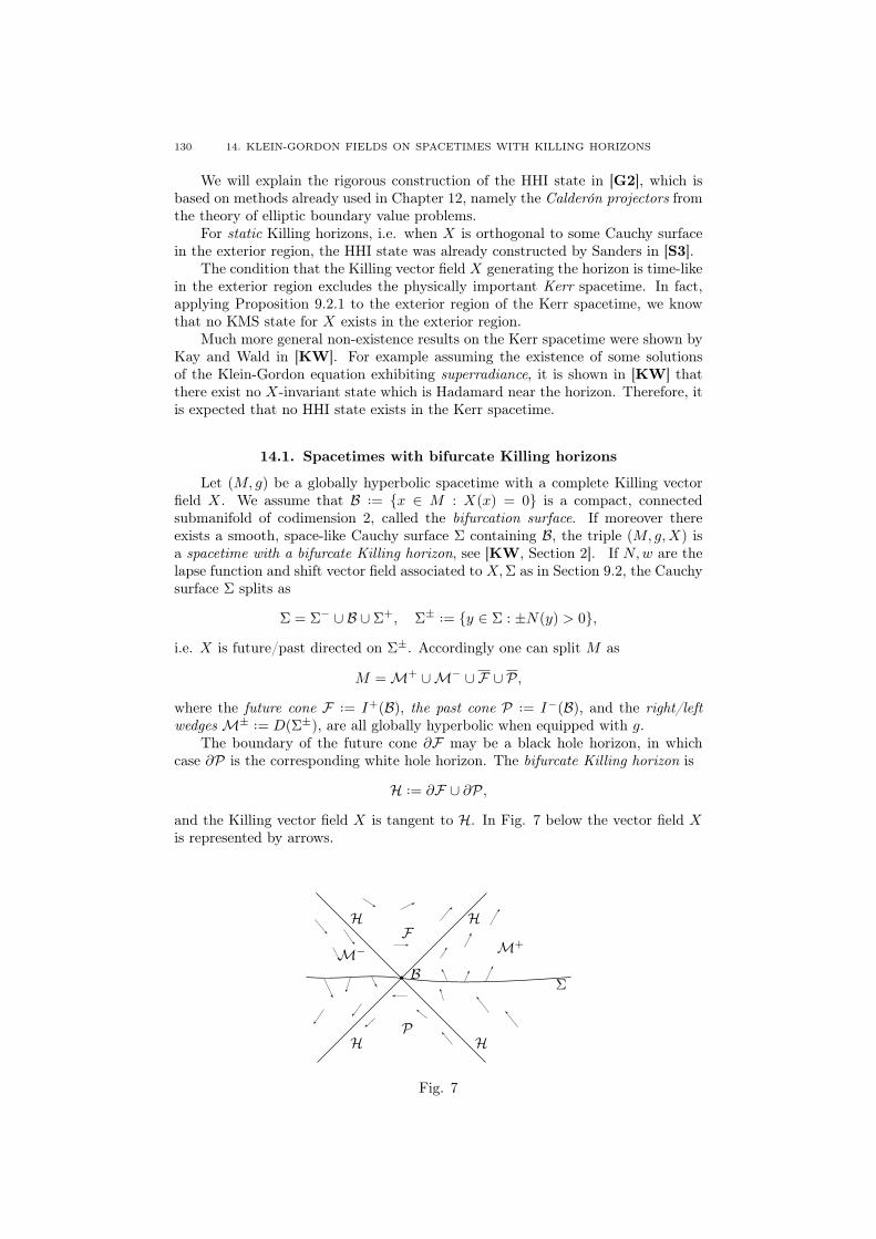
130 14. KLEIN-GORDON FIELDS ON SPACETIMES WITH KILLING HORIZONS

We will explain the rigorous construction of the HHI state in [G2], which isbased on methods already used in Chapter 12, namely the Calderón projectors fromthe theory of elliptic boundary value problems.

For static Killing horizons, i.e. when X is orthogonal to some Cauchy surfacein the exterior region, the HHI state was already constructed by Sanders in [S3].

The condition that the Killing vector field X generating the horizon is time-likein the exterior region excludes the physically important Kerr spacetime. In fact,applying Proposition 9.2.1 to the exterior region of the Kerr spacetime, we knowthat no KMS state for X exists in the exterior region.

Much more general non-existence results on the Kerr spacetime were shown byKay and Wald in [KW]. For example assuming the existence of some solutionsof the Klein-Gordon equation exhibiting superradiance, it is shown in [KW] thatthere exist no X-invariant state which is Hadamard near the horizon. Therefore, itis expected that no HHI state exists in the Kerr spacetime.

14.1. Spacetimes with bifurcate Killing horizons

Let (M, g) be a globally hyperbolic spacetime with a complete Killing vectorfield X. We assume that B ··= x ∈ M : X(x) = 0 is a compact, connectedsubmanifold of codimension 2, called the bifurcation surface. If moreover thereexists a smooth, space-like Cauchy surface Σ containing B, the triple (M, g,X) isa spacetime with a bifurcate Killing horizon, see [KW, Section 2]. If N,w are thelapse function and shift vector field associated to X,Σ as in Section 9.2, the Cauchysurface Σ splits as

Σ = Σ− ∪ B ∪ Σ+, Σ± ··= y ∈ Σ : ±N(y) > 0,

i.e. X is future/past directed on Σ±. Accordingly one can split M as

M =M+ ∪M− ∪ F ∪ P,

where the future cone F ··= I+(B), the past cone P ··= I−(B), and the right/leftwedgesM± ··= D(Σ±), are all globally hyperbolic when equipped with g.

The boundary of the future cone ∂F may be a black hole horizon, in whichcase ∂P is the corresponding white hole horizon. The bifurcate Killing horizon is

H ··= ∂F ∪ ∂P,

and the Killing vector field X is tangent to H. In Fig. 7 below the vector field Xis represented by arrows.

Σ

M+M−

F

P

HH

HH

B

Fig. 7

14.3. WICK ROTATION 131

14.1.1. The surface gravity. An important quantity associated to the Killinghorizon H is its surface gravity, defined by

κ2 = −1

2(∇bXa∇bXa)|B, κ > 0.

It is a fundamental fact, see [KW, Section 2], that the scalar κ is constant on Band actually on the whole horizon H.

14.1.2. Wedge reflection. In concrete situations, like the Schwarzschild orKerr spacetimes, the metric g is originally defined only on the right wedgeM+ andfirst extended to the future cone F by a new choice of coordinates. The regionsP,M− are constructed as copies of F ,M+, with reversed time orientation, gluedtogether along B. This motivates one to assume the existence of a wedge reflection,i.e. an isometric involution R ofM− ∪ U ∪M+, where U is a neighborhood of Bin M , such that R reverses the time orientation, R = Id on B and R∗X = X.

It can be shown, see [S3], that there exists a smooth, space-like Cauchy surfaceΣ with B ⊂ Σ such that R : Σ

∼−→ Σ. The restriction r of R to Σ is called a weakwedge reflection. We have

(14.1) r|B = Id, r : Σ±∼−→ Σ∓.

In the sequel we will fix such a Cauchy surface.

14.1.3. Stationary Killing horizons. The bifurcate Killing horizon H iscalled stationary, resp. static, if the Killing vector field X is time-like inM+, resp.time-like and orthogonal to Σ inM+.

14.2. Klein-Gordon fields

Let us consider a Klein-Gordon operator

P = −2g + V,

where V ∈ C∞(M ;R) has the same invariance properties as g, i.e. X ·V = 0,V R = V . We also strengthen the condition V > 0 in Section 9.3 to

V (x) ≥ m2, x ∈M, m > 0,

i.e. we restrict our attention to massive Klein-Gordon fields.If X is time-like in M+, we can apply Sections 9.3, Subsection 9.5 to the

Klein-Gordon operator P , on the globally hyperbolic spacetime (M+, g), withCauchy surface Σ+. We obtain, for each β > 0 the β-KMS state ωβ acting onCCRpol(C∞0 (Σ+;C2), q).

Following Section 4.8, we can associate to ωβ the doubled state ωd, which isassociated to the doubled Hermitian space

(14.2) (C∞0 (Σ+;C2)⊕ C∞0 (Σ+;C2), q ⊕−q).

14.3. Wick rotation

The key step in the construction of the Hartle-Hawking state is the inter-pretation of the double β-KMS state ωD using the Wick rotation in Killing timecoordinates. We will now explain this important step.


14.3.1. The Wick rotated metric. As in Section 9.2, we can identifyM+

with R× Σ+, the metric g taking the form

g = −N2(y)dt2 + hij(y)(dyi + wi(y)dt)(dyj + wj(y)dt),

see (9.13). As in Chapter 12, we can perform the Wick rotation, replacing theKilling time coordinate t by is. In this way we obtain from g the complex metric

geucl = N2(y)ds2 + hij(y)(dyi + iwi(y)ds

)(dyj + iwj(y)ds

).

If ξ = (τ, η) ∈ CTyM and y ∈ Σ+, then

ξ ·geucl(y)ξ = (N2(y)− w(y)·h(y)w(y))ττ + η ·h(y)η

+i(w(y)·h(y)ητ + τw(y)·h(y)η).

Since X = ∂∂t is time-like in M+, we know that N2(y) > wi(y)hij(y)wj(y), from

which we deduce that

(14.3) |Im(ξ ·geucl(y)ξ)| ≤ c(y)Re(ξ ·geucl(y)ξ), y ∈ Σ+,

for some c(y) > 0. It is convenient to have some uniformity in y in the inequality(14.3), which follows if we require that there exists δ > 0 such that

(14.4) X(y) + δw(y) is time-like for y ∈ Σ.

One can show that it suffices to assume that (14.4) holds away from a compactneighborhood of B in Σ, i.e. near spatial infinity. From (14.4) we deduce theuniform version of (14.3), namely, there exists c > 0 such that

(14.5) |Im(ξ ·geucl(y)ξ)| ≤ cRe(ξ ·geucl(y)ξ), y ∈ Σ+.

Another useful fact is that |geucl|(y) = |det geucl(y)| = N2(y)|h(y]) > 0 for ally ∈ Σ, so the density dVolgeucl = |geucl| 12 dsdy is positive.

14.3.2. The Wick rotated operator. The Klein-Gordon operator P takesthe form

P = (∂t + w∗)N−2(∂t + w) + h0,

see (9.18), and becomes after Wick rotation the differential operator

P eucl = (−∂s + iw∗)N−2(∂s + iw) + h0.

One can define the Laplace-Beltrami operator ∆geucl associated to the complexmetric geucl as in the Riemannian case and one has P eucl = −∆geucl +V (y). It alsofollows from (14.5) that P eucl is an elliptic differential operator.

Let us now associate to P eucl some densely defined operator. It is a well-knownfact that to describe quantum fields at temperature β−1 by Euclidean methods, theEuclidean time s should belong to the circle Sβ of length β.

Therefore, we set M eucl ··= Sβ × Σ+ and consider the sesquilinear form

Qβ(u, u) =

ˆMeucl

uP euclu dVolgeucl , DomQβ = C∞0 (M eucl).

It follows from (14.5) that Qβ is sectorial, i.e.,

|ImQβ(u, u)| ≤ cReQβ(u, u), u ∈ DomQβ ,

and hence closeable. The domain of its closure Qclβ equals the Sobolev space

H1(M eucl), defined as the completion of C∞0 (M eucl) with respect to the norm

‖u‖21 =

ˆMeucl

(∇u·Re(geucl)−1(y)∇u+ V (y)uu

)dVolgeucl .

By the Lax-Milgram theorem, one associates to Qclβ a boundedly invertible operator

P euclβ : H1(M eucl)

∼−→ H1(M eucl)∗,

14.4. THE DOUBLE β-KMS STATE IN M+ ∪M− 133

which corresponds to imposing β-periodic boundary conditions for the operatorP eucl.

14.3.3. Calderón projectors. Consider the open set

Ω ··= ]0, β/2[×Σ+ ⊂M eucl.

Note that ∂Ω has two connected components 0 × Σ+ and β/2 × Σ+, bothidentified with Σ+. We will use the notation introduced in Section 12.7 for spacesof distributions on Ω.

One defines the outer unit normal to ∂Ω for the complex metric geucl as theunique complex vector field ν such that

(i) ν(x)·geucl(x)v = 0, ∀v ∈ Tx∂Ω,

(ii) ν(x)·geucl(x)ν(x) = 1,

(iii) Re ν(x) is outwards pointing.

We see that ν equals −N−1( ∂∂s − iw) on 0×Σ+ and its opposite on β/2×Σ+.One can then define the trace

γu =

(u∂Ω

ν ·∇u∂Ω

)∈ C∞(∂Ω;C2)

for u ∈ C∞(Ω) with P euclu = 0 in Ω and the Calderón projectors c±β associatedto (P eucl

β ,Ω) as in Section 12.7, see [G2, Subsection 8.7] for the precise definitions.The important observation now is that the doubled state ωd constructed from ωβcan be expressed in terms of the Calderón projectors c±β . In fact one has, see [G2,Proposition 8.8]:

Proposition 14.3.1. The covariances of ωd are equal to

λ±d = ±Q (1l⊕ T )−1c±β (1l⊕ T ), Q = q ⊕ q,

where T =

(1l 00 −1l

).

Two comments are in order at this point. First, the Calderón projectors c±βare defined on C∞0 (∂Ω;C2), or equivalently on C∞0 (Σ+;C2) ⊕ C∞0 (Σ+;C2), whichis exactly the doubled phase space on which the doubled state ωd is defined.

Second the operator T takes care of the fact that ωd is associated to the Her-mitian form q ⊕−q, see (14.2), and not Q = q ⊕ q.

14.4. The double β-KMS state in M+ ∪M−

Recall that the wedge reflection R maps M+ to M− and reverses the timeorientation. It is hence easy to obtain from ωd a pure quasi-free state ωD inM+ ∪M−, called the double β-KMS state. This provides a first extension of the thermalstate ωβ inM+ to a pure state inM+ ∪M−. The Cauchy surface covariances λ±Dof ωD are the sesquilinear forms on (C∞0 (Σ+;C2), q)⊕ (C∞0 (Σ−;C2), q) given by

λ±D = ±Q (1l⊕ r∗)−1c±β (1l⊕ r∗),

where r∗f(y) = f(r(y)). Note that

RΣ = Tr∗ : (C∞0 (Σ−;C2), q)∼−→(C∞0 (Σ+;C2),−q).

is exactly the unitary map on Cauchy data induced by the wedge reflection R :C∞0 (M+)

∼−→ C∞0 (M−).


14.5. The extended Euclidean metric and the Hawking temperature

The constructions carried out up to now are valid for any β > 0. The Euclideanmetric geucl usually degenerates at the bifurcation surface B. In fact, for ω ∈ B, letnω the unit normal to B for the induced metric h on Σ, pointing towards Σ+. Usingnω one can introduce Gaussian normal coordinates (u, ω) on a neighborhood of Bin Σ, with Σ+ corresponding to u > 0. One can then show that in the coordinates(s, u, ω), the Euclidean metric geucl near u = 0 takes the form

κ2u2ds2 + du2 + k(ω)dω2,

modulo higher-order terms depending only on (u2, ω), where the Riemannian metrick(ω)dω2 is the restriction of h(y)dy2 to B, see [G2, App. A].

We recognize in the first two terms the expression of the flat Riemannian metricdX2 + dY 2, if X = u cos(κs), Y = u sin(κs), i.e. if (u, s) are polar coordinates.

Since s ∈ Sβ , we see that if β = (2π)κ−1, i.e. if β−1 equals the Hawkingtemperature κ(2π)−1, then geucl extends across B to a smooth complex metric geucl

ext ,living on a smooth manifold M eucl

ext , which near B is diffeomorphic to R2 × B. Forother values of β, no such smooth extension exists, and geucl has a conical singularityat B.

It is also important to understand the open set Ωext ⊂ M euclext corresponding

to Ω ⊂ M eucl. Its boundary ∂Ωext is obtained by gluing together along B thetwo connected components 0 × Σ+ and β/2 × Σ+ of ∂Ω. Actually, ∂Ωext isdiffeomorphic to Σ. The reason for this is that in coordinates (u, ω), the weak wedgereflection r becomes simply the reflection (u, ω) 7→ (−u, ω), and Σ+ is identifiedwith Σ− by r.

14.6. The Hartle-Hawking-Israel state

One can associate to the extended metric geuclext a Laplace-Beltrami operator

P euclext and consider its Calderón projectors c±ext for the open set Ωext.

Since the boundary ∂Ωext is diffeomorphic to Σ, it is tempting to use c±ext

to construct Cauchy surface covariances on Σ, which, if the required positivityproperties are satisfied, will define a quasi-free state on the whole of M . It turnsout that this is indeed the case, the resulting state being the sought-for Hartle-Hawking-Israel state. Let us thus summarize the main result of [G2].

In addition to the geometric assumptions explained in Section 14.1, one needsto impose some conditions on the behavior of the metric g on Σ. Namely oneassumes that there exists a neighborhood U of B in Σ such that

(H1) X + δw is time-like on Σ \ U for some δ > 0,

(H2) N−2wi ·(∇hiN), N−1∇hi wi are bounded on Σ \ U,

where we recall that h is the restriction of g to Σ, and X = Nn+w is the decompo-sition of the Killing vector field, see (9.12). To prove that the Hartle-Hawking-Israelstate is a pure state, one also needs to impose

(H3) (Σ, h) is complete.

Theorem 14.6.1. Assume hypotheses (H1)– (H3). Then:(1) λ±HHI = ±q c±ext are the Cauchy surface covariances of a quasi-free state ωHHI

for P in M , called the HHI state.(2) The restriction of ωHHI to M+ ∪ M− is the double β−KMS state ωD for

β = (2π)κ−1.(3) ωHHI is a pure Hadamard state in M .

14.6. THE HARTLE-HAWKING-ISRAEL STATE 135

(4) Let ω be a quasi-free state for P in M whose restriction toM+ ∪M− equalsωD and such that its space-time covariances map C∞0 (M) into C∞(M). Thenω = ωHHI.

Proof. Let us now explain some ingredients of the proof of Theorem 14.6.1, whichessentially relies on known results on Calderón projectors and Sobolev spaces. Werecall that Hs

loc(N), resp. Hsc (N) denote the local, resp. compactly supported

Sobolev spaces on the manifold N .Let us first check that ωHHI is indeed an extension of ωD, i.e., that λ±HHI equal

λ±D on C∞0 (Σ \ B;C2).The Calderón projectors c±ext are constructed using the inverse of P eucl

ext , whichas for P eucl is constructed from a sesquilinear form Qext. Clearly, Qext and Qβcoincide on C∞0 (M eucl

ext \ B). Near B the topology of the domain of the closure ofQext is the topology of H1

loc(M euclext ). Since B is of codimension 2 in M eucl

ext , thisimplies that C∞0 (M eucl

ext \ B) is a form core for Qext. This immediately implies thatλ±HHI and λ

±D coincide on C∞0 (Σ \ B;C2).

From this fact one can also easily deduce that λ±HHI are indeed the Cauchysurface covariances of a state, i.e., that

(14.6) λ±HHI ≥ 0, λ+HHI − λ

−HHI = q.

Let us explain this argument: it is known that Calderón projectors for second-orderelliptic operators, hence in particular c±, are continuous from H

12c (Σ)⊕H−

12

c (Σ) toH

12

loc(Σ)⊕H−12

loc (Σ). From this we deduce immediately that λ±HHI are continuous on

H12c (Σ)⊕H−

12

c (Σ).Since B is of codimension 1 in Σ, we know that the space C∞0 (Σ\B;C2) is dense

in H12c (Σ)⊕H−

12

c (Σ). The restrictions of λ±HHI to C∞0 (Σ \ B;C2) equal λ±D, and sosatisfy (14.6), since they are the Cauchy surface covariances of the state ωD. Bythe above density result, this implies that (14.6) holds on C∞0 (Σ;C2), as claimed.

To prove that ωHHI is a pure state, one would like to show that c±ext are pro-jections on some space containing C∞0 (Σ;C2) and apply Proposition 4.9.3. Thisis not obvious unless Σ is compact. Instead one can use Proposition 4.9.4 and anapproximation argument similar to the one used in [GW5, Section 4].

Further, let us explain how to prove that ωHHI is a Hadamard state. Therestriction of ωHHI to M+ is a Hadamard state for P , since it is a (2π)κ−1-KMSstate for a time-like, complete Killing vector field. The restriction of ωHHI toM−is also a Hadamard state for P .

This implies that the restriction of ωHHI to M+ ∪M− is a Hadamard state.The same is true of the restriction of a reference Hadamard state ωref in M (seeTheorem 11.8.1) toM+∪M−. Passing to Cauchy surface covariances on Σ+∪Σ−,this implies that if χ ∈ C∞0 (Σ±), then χ (λ±HHI−λ

±ref) χ is a smoothing operator

on Σ. This implies that λ±HHI − λ±ref is smoothing, which shows that ωHHI is aHadamard state.

If fact let a be one of the entries of λ±HHI − λ±ref , which is a scalar pseudodif-

ferential operator belonging to Ψm(Σ) for some m ∈ R. We know that χ a χis smoothing for any χ ∈ C∞0 (Σ\B). Then its principal symbol σpr(a) vanishes onT ∗(Σ\B) hence on T ∗Σ by continuity, so a ∈ Ψm−1(Σ). Iterating this argument,we obtain that a is smoothing.

For the proof of the uniqueness statement (3) we refer the reader to [G2]. 2

CHAPTER 15

Hadamard states and scattering theory

In this chapter we study the construction of Hadamard states from scatteringdata, i.e., from data at future or past time infinity. This construction is related tothe construction of Hadamard states from past or future null infinity on asymptot-ically flat spacetimes, which we reviewed in Chapter 13. The geometric assumptionon the spacetime (M, g) is that it should be asymptotically static, at past or futuretime infinity, see Section 15.1. Roughly speaking, this means that M should be ofthe form R×Σ and g should tend to a standard static metric gout/in, see Subsections5.3.3, when t→ ±∞.

The existence of the out and in vacuum states ωout/in for a Klein-Gordon opera-tor P on (M, g), i.e., of states looking like the Fock vacua for the static Klein-Gordonoperators Pout/in on (M, gout/in) at large positive or negative times, is often takenfor granted in the physics literature.

We will explain the result of [GW3], which provides a proof of the existenceof ωout/in and more importantly of their Hadamard property.

15.1. Klein-Gordon operators on asymptotically static spacetimes

Let us now introduce a class of spacetimes that are asymptotically static atfuture and past time infinity and corresponding Klein-Gordon operators We fix an(n−1)-dimensional manifold Σ and set M = Rt×Σy, y = (t, y). We equip M withthe Lorentzian metric

(15.1) g = −c2(y)dt2 +(dyi + bi(y)dt

)hij(y)

(dyj + bj(y)dt

),

where c ∈ C∞(M), h(t, y)dy2, resp. b(t, y) is a smooth t-dependent Riemannianmetric, resp. vector field on Σ.

If there exist a reference Riemannian metric k(y)dy2 on Σ and constants c0, c1 >0 such that(15.2)

h(t, y) ≤ c1k(y), b(t, y)·h(t, y)b(t, y) ≤ c1, c0 ≤ c(t, y) ≤ c1, (t, y) ∈M,

then it follows from [CC, Theorem 2.1] that t : M → R is a Cauchy temporalfunction for (M, g), see Definition 5.4.5, hence in particular (M, g) is globally hy-perbolic.

It is natural to use the framework of bounded geometry and to equip Σ witha reference Riemannian metric k such that (Σ, k) is of bounded geometry. Theversion of (15.2) is then

(15.3) (bg)

h ∈ C∞b (R;BT 0

2 (Σ, k)), h−1 ∈ C∞b (R;BT 20 (Σ, k)),

b ∈ C∞b (R;BT 10 (Σ, k)) c, c−1 ∈ C∞b (R;BT 0

0 (Σ, k)).

A concrete example of (Σ, k) is Rd equipped with the uniform metric.

15.1.1. Asymptotically static spacetimes. Let us consider a Klein-Gordonoperator

P = −(∇µ − iqAµ(x))(∇µ − iqAµ(x)) + V (x)

137

138 15. HADAMARD STATES AND SCATTERING THEORY

on (M, g). We now impose conditions on h, b, c, A, V which mean that (M, g) isasymptotically static at t = ±∞. Let us first introduce a convenient notation.

Definition 15.1.1. Let F be a Fréchet space whose topology is defined by thesemi-norms ‖ · ‖n, n ∈ N. For I ⊂ R an interval, we denote by Sδ(I;F), δ ∈ R,the space of functions I 3 t 7→ X(t) ∈ F such that

supt∈I〈t〉−δ+m‖∂mt X(t)‖n <∞, ∀m,n ∈ N.

We introduce two static metrics

gout/in = −c2out/in(y)dt2 + hout/in(y)dy2

and time-independent potentials Vout/in and assume the following conditions

(as)

h(y)− hout/in(y) ∈ S−µ(R±;BT 02(Σ, k)),

b(y) ∈ S−µ′(R;BT 10(Σ, k)), A(y) ∈ S−µ′(R;BT 0

1(Σ, k)),

c(y)− cout/in(y) ∈ S−µ(R±;BT 00(Σ, k)),

V (y)− Vout/in(y) ∈ S−µ(R±;BT 00(Σ, k)),

for some µ > 0, µ′ > 1. Here the space Sδ(R;BT pq (Σ, k)), δ ∈ R is defined as inDefinition 15.1.1.

The above conditions are standard scattering type conditions, with µ, µ′ mea-suring the rate of convergence of h, b, etc. to their limits at t = ±∞. The conditionµ′ > 1 is traditionally called a short-range condition in the scattering theory forSchrödinger equations, while µ > 0 corresponds to the weaker long-range condition.

15.2. The in and out vacuum states

15.2.1. The asymptotic Klein-Gordon operators. It follows from condi-tion (as) that when t→ ±∞, P is asymptotic to the Klein-Gordon operator

Pout/in = −2gout/in+ Vout/in,

associated to the static metric gout/in. We can introduce the ultra-static metric

gout/in = c−2out/ingout/in = −dt2 + hout/in(y)dy

and obtain from Section 6.3 that

Pout/in = c−n/2−1out/in Pout/inc

n/2−1out/in ,

where

Pout/in = −2gout/in+

n− 2

4(n− 1)Scalgout/in

+ c−2out/inVout/in,

and Vout/in = Vout/in − n−24(n−1)Scalgout/in

. The ultra-static Klein-Gordon operatorPout/in equals ∂2

t + aout/in(y, ∂y), and to avoid technical complications coming frominfrared problems we will assume that

(pos)n− 2

4(n− 1)Scalgout/in

+ c−2out/inVout/in ≥ m2, for some m > 0,

which simply means that

aout/in ≥ m2 > 0 on L2(Σ, |hout/in|12 (y)dy),

for hout/in = c−2out/inhout/in.

15.2. THE IN AND OUT VACUUM STATES 139

It follows that Pout/in admits a vacuum state ωvacout/in, see Subsection 4.10.2,

whose Cauchy surface covariances are

λ±,vacout/in =

1

2

(εout/in ±1l±1l ε−1

out/in

), εout/in = a

12

out/in.

By Subsection 6.3.2, Pout/in admit the vacuum state ωvacout/in, whose Cauchy surface

covariances on Σ0 = 0 × Σ are

λ±,vacout/in = (U∗out/in)−1 λ±,vac

out/in U−1out/in, U =

(c1−n/2out/in 0

0 c−n/2out/in

).

15.2.2. The out and in vacuum states. We have seen that Σs = s × Σare Cauchy surfaces for (M, g). Denoting by %s : Solsc(P ) → C∞0 (Σs;C2) theCauchy data map on Σs, see (5.27) and by Usf , f ∈ C∞0 (Σs;C2), the solution ofthe Cauchy problem on Σs we set

U(t, s) ··= %tUs : C∞0 (Σs;C2) −→ C∞0 (Σt;C2).

If ω is a quasi-free state for P , with spacetime covariances Λ±, we will denote byλ±t its Cauchy surface covariances on Σt, called the time t covariances of the stateω.

From Propositions 5.5.4, 6.1.6 it easily follows that

(15.4) λ±s = U(t, s)∗ λ±t U(t, s), s, t ∈ R.We would like to define quasi-free states ωout/in for P , called the out/in vacua

which look like the ‘free’ vacua ωvacout/in when t→ ±∞. Taking (15.4) into account,

we see that ωout/in should be defined by the time 0 covariances:

(15.5) λ±out/in(0) = limt→±∞

U(t, 0)∗ λ±,vacout/in U(t, 0),

where the limit above is taken as sesquilinear forms on C∞0 (Σ0;C2). Of course, thereference time t = 0 is completely arbitrary.

The following theorem is the main result of [GW3].

Theorem 15.2.1. Assume the conditions (bg), (as) and (pos). Then:(1) the limits (15.5) when t→ +∞, resp. −∞, exist and are the time 0 covariances

of a quasi-free state for P denoted by ωout, resp. ωin, called the out resp. invacuum state.

(2) ωout/in are pure Hadamard states.

15.2.3. Wave operators. The static vacua ωvacout/in are invariant under time

translations: if Uout/in(t, s) is the Cauchy evolution operator for Pout/in, thenUout/in(t, s) = Uout/in(t+ T, s+ T ) and

λ±,vacout/in = Uout/in(t, s)∗ λ±,vac

out/in Uout/in(t, s).

Therefore we can rewrite (15.5) as

λ±out/in(0) = limt→±∞

(Uout/in(0, t) U(t, 0))∗ λ±,vacout/in (Uout/in(0, t) U(t, 0)).

If the exponent µ in conditions (as) satisfies µ > 1, then one can prove that thestrong limits

(15.6) Wout/in = s− limt→±∞

Uout/in(0, t) U(t, 0)

exist on some natural energy spaces. The operators Wout/in are called (inverse)wave operators and (15.5) takes the more familiar form

λ±out/in(0) = W ∗out/inλ±,vacout/inWout/in,


which is often found in the physics literature. Note however that the existence ofWout/in requires µ > 1, while the existence of ωout/in only requires µ > 0.

15.3. Reduction to a model case

We now give some ideas of the proof of Theorem 15.2.1. The existence of ωout/in,at least in the short-range case µ > 1, is not very difficult, using the argumentsoutlined in Subsection 15.2.3.

The Hadamard property is more delicate. For example, the covariances U(t, 0)∗λ±,vac

out/in U(t, 0) in the right-hand side of (15.5) are not Hadamard for P for finitet. In fact, the free vacua ωvac

out/in are Hadamard states for Pout/in, but not for P . Itis only after taking the limit t→∞ that one obtains a Hadamard state for P .

The proof of Theorem 15.2.1 is done by reduction to a model case, similar tothe one considered in Section 11.2. Since we want to use the time coordinate tand not the Gaussian time, we use the orthogonal decomposition associated to texplained in Subsection 5.4.1.

15.3.1. Orthogonal decomposition. One can identify 0 × Σ with Σ anduse the vector field

v = (∇t·g∇t)−1∇t = ∂t + bi(y)∂yi

as in Subsection 5.4.1 to construct an orthogonal decomposition of g by the diffeo-morphism

χ : R× Σ 3 (t, x) 7−→ (t, y(t, 0, x)) ∈ R× Σ,

where y(t, s, ·) : Σ→ Σ is the flow of the time-dependent vector field bi(y)∂yi on Σ.The metric χ∗g takes the form

χ∗g = c2(t, x)dt2 + h(t, x)dx2.

After a further conformal transformation, the operator

P ··= c1−n/2χ∗P c1+n/2

take on the form, see [GW3, Subsection 5.2]

P = ∂2t + r(t, x)∂t + a(t, x, ∂x),

i.e. is a model Klein-Gordon operator of the type considered in Section 11.2.

15.3.2. Properties of the model operator. In the sequel the model oper-ator P will be denoted by P for simplicity.

Let us first introduce classes of time-dependent pseudodifferential operatorson Σ that are analogs of the classes of time-dependent tensors Sδ(R;BT pq (Σ, k))defined in Subsection 15.1.1. We set

Ψm,δtd (I; Σ) ··= Op(Sδ(I;BSmph(Σ))) + Sδ(I;W−∞(Σ)),

where BSmph(Σ) and W−∞(Σ) are defined in Definitions 10.4.1, 10.4.3, and we useDefinition 15.1.1.

One can show that the conditions (bg), (as), (pos) imply the conditions

(td)

a(t, x, ∂x) = aout/in(x, Dx) + Ψ2,−δ

td (R±; Σ), δ > 0,

r(t) ∈ Ψ0,−1−δtd (R; Σ),

aout/in(x, ∂x) ∈ Ψ2(Σ) elliptic, aout/in(x, Dx) = aout/in(x, Dx)∗ ≥ C∞ > 0,

for δ = min(µ, µ′ − 1). The asymptotic Klein-Gordon operators are now

Pout/in = ∂2t + aout/in(x, ∂x).

15.3. REDUCTION TO A MODEL CASE 141

The decay conditions (td) lead to an improvement of the properties of thegenerator b(t) constructed in Section 11.3. Indeed, setting ε(t) = a(t, x, ∂x)

12 and

εout/in = a12

out/in one can show that b(t) in Proposition 11.3.1 can be chosen so that

(15.7)b(t) = ε(t) + Ψ0,−1−δ

td (R;±Σ) = εout/in + Ψ1,−δtd (R±; Σ),

i∂tb− b2 + a+ irb ∈ Ψ−∞,−1−δtd (R; Σ).

15.3.3. Almost diagonalization. In Chapter 11 the microlocal splitting de-duced from a solution b(t) was used to construct a pure Hadamard state. It isalso possible, see [GOW, Section 6], to use it to diagonalize the evolution U(t, s)associated to P , modulo smoothing error terms. Let us set

T (t) ··= i−1

(1l −1lb+ −b−

)(b+ − b−)−

12 (t),

where we recall that b+(t) = b(t), b−(t) = −b∗(t). Then one can check that

T−1(t) = i(b+ − b−)−12

(−b− 1l−b+ 1l

)(t).

We now define

(15.8) U(t, s) =·· T (t) Uad(t, s) T (s)−1, t, s ∈ R

which is (at least formally) a two-parameter group. Computing the infinitesimalgenerator of Uad(t, s)t,s∈R one obtains

(15.9) Had(t) =

(−b− + r−b 0

0 −b+ + r+b

)(t) +R−∞(t),

where R−∞ ∈ Ψ−∞,−1−δtd (R; Σ) ⊗ M(C2) and r±b ∈ Ψ0,−1−δ

td (R; Σ), i.e. Had(t)is diagonal, modulo the regularizing in space and decaying in time error termR−∞(t). There is a similar well-known exact diagonalization of the Cauchy evolu-tions Uout/in(t, s) for Pout/in. If

Tout/in = (i√

2)−1

ε− 1

2

out/in −ε−12

out/in

ε12

out/in ε12

out/in

, εout/in = a12

out/in,

thenUout/in(t, s) = Tout/in Uad

out/in(t, s) T−1out/in,

and the (time-independent) generator Hadout/in of Uad

out/in(t, s) equals

Hadout/in =

(εout/in 0

0 −εout/in

).

The vacua ωvacout/in are pure states associated to the projections

c±out/in = Tout/in π+ T−1out/in, for π+ =

(1l 00 0

), π− = 1l− π+.

Rather straightforward arguments show that the existence of the limits in Theorem15.2.1 follows from the existence of

(15.10) limt→±∞

Wout/in(t)π±Wout/in(t)−1, for Wout/in(t) = Uad(0, t)Uadout/in(t, 0),

for example in B(L2(Σ;C2)). Using the properties of Had(t) one can actually provethat

(15.11) s− limt→±∞

Wout/in(t) π± Wout/in(t)−1 = π± +W−∞(Σ)⊗M(C2).


This implies not only the existence of the out/in vacuum states, but also theirHadamard property. Indeed, if c± = T (0)π±T (0)−1 then λ±(0) = ±q c± arethe Cauchy surface covariances on Σ0 of the Hadamard state associated to themicrolocal splitting obtained from b, see Section 11.4. From (15.11) we obtain thatλ±out/in(0) differ from λ±(0) by a smoothing error, which proves that ωout/in areHadamard states.

CHAPTER 16

Feynman propagator on asymptotically Minkowskispacetimes

We have seen in Section 7.4 that a Klein-Gordon operator P on a globally hyper-bolic spacetime (M, g) possesses four distinguished parametrices, the retarded/advancedparametrices Gret/adv and the Feynman/anti-Feynman parametrices GF/F, uniquemodulo smooth kernels and uniquely characterized by the wavefront set of theirdistributional kernels.

One can ask if there exist true inverses of P , corresponding to the above para-metrices and canonically associated to the spacetime (M, g).

By Lemma 7.4.3, there exists true retarded/advanced inverses of P , namelyGret/adv, see Theorem 5.5.1, which are uniquely determined by the causal structureof (M, g).

The situation is more complicated for the Feynman/anti-Feynman inverses. Ofcourse, given a Hadamard state ω for P , the Feynman inverse associated to ω, see(8.14), has the correct wavefront set, but it depends on the choice of the Hadamardstate ω, and hence is not canonical.

There are some situations where such a canonical Feynman inverse exists. If(M, g) is stationary with Killing vector field X and P is invariant under X, one can,under the conditions in Chapter 9, construct the vacuum state ωvac associated toX and the corresponding Feynman inverse GF is a canonical choice of a Feynmaninverse, respecting the symmetries of (M, g).

In the particular case of the Minkowski spacetime R1,d and P = ∂2t − ∆x +

m2, the Feynman inverse obtained from the vacuum state is equal to the Fouriermultiplier by the distribution

−1

τ2 − (k2 +m2) + i0.

In this chapter we will describe the results of [GW4, GW6], devoted to thisquestion on spacetimes which are asymptotically Minkowski, and hence have ingeneral no global symmetries, only asymptotic ones.

It turns out that it is possible in this case to define a canonical Feynman inverseGF, which is the inverse of P between some appropriate Sobolev type spaces.

More concretely, one introduces spaces Ym, XmF for m ∈ R, see Section 16.3,where Ym is a space of functions decaying fast enough when t → ±∞, while thefunctions in XmF satisfy asymptotic conditions at t = ±∞ which are analogs of thewavefront set condition which characterizes Feynman parametrices.

One can show that P : XmF → Ym is invertible, and that its inverse GF is aFeynman parametrix in the sense of Subsection 7.4.2.

Vasy [Va] considered the same problem by working directly on the scalar oper-ator P using microlocal methods. He constructed the Feynman inverse GF betweenmicrolocal Sobolev spaces, as the boundary value (P − i0)−1 of the resolvent of P .

143

144 16. FEYNMAN PROPAGATOR ON ASYMPTOTICALLY MINKOWSKI SPACETIMES

16.1. Klein-Gordon operators on asymptotically Minkowski spacetimes

In this subsection we recall the framework considered in [GW4].

16.1.1. Asymptotically Minkowski spacetimes. We consider M = R1+d

equipped with a Lorentzian metric g such that

(aM(i)) gµν(x)− ηµν ∈ S−δstd(R1+d), δ > 1,

(aM(ii)) (R1+d, g) is globally hyperbolic,

(aM(iii)) (R1+d, g) has a temporal function t with t− t ∈ S1−εstd (R1+d) for ε > 0,

where ηµν is the Minkowski metric and Sδstd(R1+d) denotes the class of smoothfunctions f such that, for 〈x〉 = (1 + |x|) 1

2 ,

∂αx f ∈ O(〈x〉δ−|α|), α ∈ N1+d.

Recall that t is called a temporal function if ∇t is a time-like vector field, and iscalled a Cauchy temporal function if in addition its level sets are Cauchy surfacesfor (M, g).

It is shown in [GW4] that if (aM(i)) holds, then (aM(ii)) is equivalent to thefamiliar non trapping condition for null geodesics of g, and if (aM(i), (ii), (iii)) hold,then there exists a Cauchy temporal function t such that t− t ∈ C∞0 (M).

Replacing t by t − c, t by t − c for c 1 we can also assume that Σ ··= t =0 = t = 0 is a Cauchy surface for (M, g), which can be canonically identifiedwith Rd. In the sequel we will fix such a temporal function t.

16.1.2. Klein-Gordon operator. We fix a real function V ∈ C∞(M ;R)such that

(aM(iv)) V (x)−m2 ∈ S−δstd(R1+d), for some m > 0, δ > 1,

and consider the Klein-Gordon operator

P = −2g + V.

16.2. The Feynman inverse of P

We now introduce the Hilbert spaces XmF , Ym between which P will be invert-ible. The spaces Ym are standard spaces of right-hand sides for the Klein-Gordonequations, their essential property being that their elements are L1 in t, with val-ues in some Sobolev spaces of order m. The spaces XmF incorporate the Feynmanboundary conditions, which are imposed at t = ±∞.

16.2.1. Hilbert spaces. Using the Cauchy temporal function t we can iden-tify M with R×Σ using the flow φt of the vector field v = g−1dt

dt·g−1dt, and obtain the

diffeomorphism

(16.1) χ : R× Σ 3 (t, x) 7−→ φt(x) ∈M,

such thatχ∗g = −c2(t, x)dt2 + h(t, x)dx2.

For m ∈ R we denote by Hm(Rd) the usual Sobolev spaces on Rd. We set, for12 < γ < 1

2 + δ

Ym ··= u ∈ D′(M) : χ∗u ∈ 〈t〉−γL2(R;Hm(Rd)),with norm ‖v‖Ym = ‖χ∗u‖L2(R;Hm(Rd)). The exponent γ is chosen such that〈t〉−γL2(R) ⊂ L1(R). Similarly we set

Xm ··= u ∈ D′(M) : χ∗u ∈ C0(R;Hm+1(Rd)) ∩ C1(R;Hm(Rd)), Pu ∈ Ym.

16.3. CONSTRUCTION OF THE FEYNMAN INVERSE 145

We equip Xm with the norm

‖u‖Xm = ‖%0u‖Em + ‖Pu‖Ym ,

where %su =

(uΣs

i−1∂nuΣs

)is the Cauchy data map on Σs ··= t−1(s) and

Em ··= Hm+1(Rd)⊕Hm(Rd) is the energy space of orderm. From the well-posednessof the inhomogeneous Cauchy problem for P one easily deduces that Xm is a Hilbertspace.

16.2.2. Feynman boundary conditions. Let us set

c±free =1

2

(1l ±

√−∆x +m2

±√−∆x +m2 1l

).

Of course, λ±free = ±q c±free for q =

(0 1l1l 0

)are the Cauchy surface covariances

on Σ of the free vacuum state ωfree associated to Pfree. We set then

XmF ··= u ∈ Xm : limt→∓∞

c±free%tu = 0 in Em.

It is easy to see that XmF is a closed subspace of Xm.The following theorem is proved in [GW6].

Theorem 16.2.1. Assume (aM). Then P : XmF → Ym is boundedly invertiblefor all m ∈ R. Its inverse GF is called the Feynman inverse of P . It satisfies

WF(GF)′ = ∆ ∪ CF.

We recall that CF was defined in Section 7.4. In particular GF is a Feynmanparametrix for P .

16.3. Construction of the Feynman inverse

We now give some ideas of the proof of Theorem 16.2.1. As in Section 15.3,the first step consists in the reduction to a model Klein-Gordon equation, by usingsuccessively the diffeomorphism χ in Subsection 16.2.1 and the conformal transfor-mation χ∗g → c−2(t, x)χ∗g. After this reduction, we work on R1+d with elementsx = (t, x) equipped with the Lorentzian metric

g = −dt2 + hij(t, x)dxidxj ,

where t 7→ ht = hij(t, x)dxidxj is a smooth family of Riemannian metrics on Rd.The Klein-Gordon operator P = −2g + V takes the form

(16.2) P = ∂2t + r(t, x)∂t + a(t, x, ∂x),

wherea(t) = a(t, x, ∂x) = −|h|− 1

2 ∂ihij |h| 12 ∂j + V (t, x),

r(t) = r(t, x) = |h|− 12 ∂t(|h|

12 )(t, x).

The operator a(t) is formally selfadjoint for the time-dependent scalar product

(u|v)t =

ˆΣ

uv|ht|12 dx,

and P is formally selfadjoint for the scalar product

(u|v) =

ˆR×Σ

uv|ht|12 dxdt.


Conditions (aM) on the original metric g and potential V imply similar asymptoticconditions on a(t, x, ∂x) and r(t, x) when t→ ±∞. More precisely, one has

(Hstd)

a(t, x, ∂x) = aout/in(x, ∂x) + Ψ2,−δstd (R±;Rd),

r(t) ∈ Ψ0,−1−δstd (R;Rd),

aout/in(x, ∂x) ∈ Ψ2,0sc (Rd) is elliptic,

aout/in(x, ∂x) = aout/in(x, ∂x)∗ ≥ C∞ > 0,

where Ψm,δstd (R±;Rd) is the class of time-dependent pseudodifferential operators on

Rd associated to symbols m(t, x, k) such that

∂γt ∂αx ∂

βkm(t, x, k) ∈ O((〈t〉+ 〈x〉)δ−γ−|α|〈k〉m−|β|), γ ∈ N, α, β ∈ Nd, t ∈ R±.

Similarly, Ψm,δsc (Rd) is the class of pseudodifferential operators on Rd associated to

symbols m(x, k) such that

∂αx ∂βkm(x, k) ∈ O(〈x〉δ|α|〈k〉m−|β|), α, β ∈ Nd.

We refer the reader to [GW4, Subsection 2.3] for more details.The Hilbert spaces Ym and Xm become

Ym = 〈t〉−γL2(R;Hm(Rd)),

Xm = u ∈ C0(R;Hm+1(Rd)) ∩ C1(R;Hm(Rd)) : Pu ∈ Ym,

equipped with the norm

‖u‖2Xm = ‖%0u‖2Em + ‖Pu‖2Ym ,

where %tu =

(u(t)

i−1∂tu(t)

)and the energy space Em is defined in Subsection 16.2.1.

The subspaces XmF become

XmF ··= u ∈ Xm : limt→−∞

c−out%tu = limt→+∞

c+in%tu = 0 in Em

where

c±out/in =1

2

1 ±a12

out/in

±a12

out/in 1

are the projections for the out/in vacuum state ωout/in associated to the Klein-Gordon operator ∂2

t + aout/in(x, ∂x).

16.3.1. A further reduction. It is convenient to perform a further reductionto the case r = 0. Namely, setting R = |h0|

14 |ht|−

14 , we see that

L2(Σ, |h0|12 dx) 3 u 7−→ Ru ∈ L2(Σ, |ht|

12 dx)

is unitary and thatR−1PR =·· P = ∂2

t + a(t, x, ∂x),

wherea(t) = rR−1∂tR+R−1(∂2

tR) +R−1a(t)R

is formally selfadjoint for (·|·)0. Clearly, a(t, x, ∂x) satisfies also (Hstd), with thesame asymptotic aout/in(x, ∂x). It is also immediate that the Hilbert spaces Ym,Xm and XmF introduced in Section 2.2 are invariant under the map u 7→ Ru andhence we can assume that r(t, x) = 0.


16.3.2. Almost diagonalization. One can then perform the same almostdiagonalization as in Subsection 15.3.3. The stronger spacetime decay in conditions(Hstd) give stronger decay conditions on the off diagonal terms. More precisely, if

H(t) =

(0 1la(t) 0

)is the generator of the Cauchy evolution for P and T (t) is as

in Subsection 15.3.3 we have

T−1(Dt −H(t))T = Dt −Had(t) =·· P ad,

where Had(t) is almost diagonal, i.e.

Had(t) = Hd(t) + V ad−∞(t),

(16.3) Hd(t) =

(ε+(t) 0

0 ε−(t)

),

where ε±(t) belong to Ψ1,0(R;Rd), with principal symbols equal to ±(k·h−1(t, x)k)12 ,

and V ad−∞(t) is an off-diagonal matrix of time-dependent operators on Rd such that

(16.4) (〈x〉+ 〈t〉)mV ad−∞(t)(〈x〉+ 〈t〉)−m+δ : H−p(Rd) −→ Hp(Rd)

is uniformly bounded in t for all m, p ∈ R. Compared with the situation in Section15.3, we obtain extra decay in x and hence compactness properties of V ad

−∞.We denote by U(t, s), resp. Uad(t, s), for t, s ∈ R, the Cauchy evolution gener-

ated by H(t), resp. Had(t). Recall from (15.8) that

(16.5) U(t, s) = T (t) Uad(t, s) T (s)−1.

Moreover, U(t, s)(ad) are unitary with respect to the Hermitian scalar product

(16.6) f ·q(ad)g = (f |q(ad)g)H0 , q =

(0 1l1l 0

), qad ··=

(1l 00 −1l

)where H0 = L2(Rd, |h0|

12 dx;C2), which implies the identity

(16.7) Had(t)∗qad = qadHad(t),

where the adjoint is computed with respect to the scalar product of H0.The spaces corresponding to Ym, XmF with the scalar operator P replaced by

the matrix operator Dt −Had(t) are the following:

Yad,m = 〈t〉−γL2(R,Hm),

X ad,m = uad ∈ C0(R;Hm+1) ∩ C1(R;Hm) : P aduad ∈ Yad,m,equipped with the norm

‖uad‖2X ad,m = ‖%0uad‖2Hm + ‖P adu‖2Yad,m ,

where Hm = Hm(Rd) ⊕ Hm(Rd) and %adt u

ad = uad(t). The subspace X ad,mF is

defined as

X ad,mF

··= uad ∈ X ad,m : limt→−∞

π+%adt u

ad = limt→+∞

π−%adt u

ad = 0 in Hm,

where

π+ =

(1 00 0

), π− =

(0 00 1

).

Note that π± are the spectral projections on R± for the Hamiltonian

Hadout/in =

a12

out/in 0

0 −a12

out/in

and we will denote by Uad

out/in(t, s) the evolution generated by Hadout/in.


Proposition 16.3.1. Assume (aM). Then the operator P ad : X ad,mF → Ym is

Fredholm of index 0.

Proof. Set P d = Dt −Hd(t). Then P d : X ad,mF → Yad,m is boundedly invertible,

with inverse GdF given by

GdFv

ad(t) ··= i

ˆ t

−∞Ud(t, 0)π+Ud(0, s)vad(s)ds

− i

ˆ +∞

t

Ud(t, 0)π−Ud(0, s)vad(s)ds.

It is easy to show, see [GW4, Lemma 3.7], that V ad−∞ is compact from X ad,m to

Ym, hence also from X ad,mF to Ym since X ad,m

F is closed in X ad,m. 2

Now let us prove that P ad : X ad,mF → Ym is injective, and hence boundedly

invertible by Proposition 16.3.1. The proof of Lemma 16.3.2 below is inspired bythe work of Vasy [Va, Proposition 7], which in turn relies on arguments of Isozaki[I] from N -body scattering theory.

Lemma 16.3.2. One has:

KerP ad|X ad,mF

= 0 for all m ∈ R.

Proof. We first note that if uad ∈ KerP ad|X ad,mF

, we have uad = −GdFV

ad−∞u

ad,

from which we deduce that uad ∈ X ad,m′

F for any m′, using that V ad−∞ is smoothing

in x. Therefore, it suffices to prove the lemma for m ≥ 1.Let us set χε(t) =

´ +∞|t| 1l[1,2](εs)s

−rds for some 0 < r < 1. Note that suppχε ⊂|t| ≤ 2ε−1. Let us still denote by χε the operator χε ⊗ 1lC2 . Recalling that qad isdefined in (16.6), we compute for u ∈ X ad,m

F :ˆR

(P aduad(t)|qadχε(t)u

ad(t))H0 −

(χε(t)u

ad(t)|qadP aduad(t))H0dt

=

ˆR

(Dtu

ad(t)|qadχε(t)uad(t)

)H0 −

(uad(t)|qadχε(t)Dtu

ad(t))H0dt

+

ˆR

(uad(t)|qad[Had(t), χε(t)]u

ad(t))H0dt,

using that Had∗(t)qad = qadHad(t), χε(t)∗qad = qadχε(t) and uad(t) ∈ DomHad(t)since m ≥ 1. We have [Had(t), χε(t)] = 0, and since χε is compactly supported int we can integrate by parts in t in the second line and obtain(16.8) ˆ

R

(P aduad(t)|qadχε(t)u

ad(t))H0dt−

ˆR

(χε(t)u

ad(t)|qadP aduad(t))H0dt

= −i

ˆR

(uad(t)|qad∂tχε(t)u

ad(t))H0dt.

Note that we used here that the scalar product in H0 does not depend on t, whichis the reason for the reduction to r = 0 in Subsection 16.3.1.

Since P aduad = 0, this yields

(16.9)ˆR


ad(t))H0dt = 0.

We claim that:

(16.10)(i) ‖π±uad(t)‖2H0 ∈ O(t1−δ), when t→ ∓∞,

(ii) ‖π±uad(t)‖2H0 = c± +O(t1−δ), when t→ ±∞,


for c± = limt→± ‖π±uad(t)‖2H0 . The proof of (16.10) is elementary: we haveHad(t) − Had

out/in ∈ O(t−δ) in B(H0) when t → ±∞, see e.g. [GW1, Subsection2.5], which using that δ > 1 and the Cook argument yields

W †out/inuad = limt→± Uad

out/in(0, t)uad(t) exists in H0,

‖W †out/inuad − Uad

out/in(0, t)uad(t)‖H0 ∈ O(t1−δ).

Since Uadout/in(0, t) is unitary on H0, this yields (16.10). We then computeˆR


ad(t))H0dt

=

ˆR∂tχε(t)‖π+uad(t)‖2H0dt−

ˆR∂tχε(t)‖π−uad(t)‖2H0dt =·· I+ + I−.

Since ∂tχε(t) = −sgn(t)1l[ε−1,2ε−1](|t|)|t|−r, we have, using (16.10):

0 ≤ˆR∓|∂tχε(t)|‖π±uad(t)‖2H0dt ≤ C

ˆ1l[ε−1,2ε−1](|t|)|t|−r−δ+1dt ∈ O(εr+δ−2),

ˆR±

∂tχε(t)‖π±uad(t)‖2H0dt = ∓ˆR±

1l[ε−1,2ε−1](|t|)c+|t|−rdt+O(εr+δ−2)

= ∓Cc±εr−1 +O(εr+δ−1).

Using (16.9), this yields Cεr−1(c+ + c−) ∈ O(εr+δ−2), hence c+ = c− = 0, sinceδ > 1. Therefore by (16.10) we have limt→±∞ ‖uad(t)‖H0 = 0. Since the Cauchyevolution Uad(t, s) is uniformly bounded in B(H0) we have uad(0) = 0, hence u = 0.2

The reduction explained at the beginning of Section 16.3 shows that Theorem16.2.1 follows from

Theorem 16.3.3. P : XmF → Ym is boundedly invertible, with inverse

GF = −π0TGadF T−1π∗1 .

Moreover, GF is a Feynman inverse of P , i.e.

(16.11) WF(GF)′ = ∆ ∪ CF.

Proof. It is straightforward using the expression of T to check that

π0T ∈ B(X ad,m+ 12 ,Xm), T−1π∗1 ∈ B(Ym,Yad,m+ 1

2 ),

and so GF : Ym → Xm. Since (Dt −H(t))TGadF T−1 = TGad

F T−1(Dt −H(t)) = 1l,we obtain that PGF = GFP = 1l. We have also %π0TG

adF T−1π∗1 = TGad

F T−1π∗1v.From [GW4, equ. (3.25)] we obtain that π0T : X ad,m+ 1

2

F → XmF , hence %FGF = 0,i.e. GF : Ym → XmF .

To prove the second statement, let GF = −π0TGdFT−1π∗1 . We have Gd

F−GadF =··

R−∞ = GdFV

ad−∞G

adF by the resolvent identity. It is shown in [GW1, Lemma 3.7]

that V ad−∞ : X ad,m → Ym′ is bounded for all m′ > m, hence R−∞ : Yad,m → X ad,m′

for all m′ > m, i.e. is smoothing in the x variables. We use then that DtR−∞ =Hd(t)R−∞+V ad

−∞GadF , R−∞Dt = R−∞H

ad(t) +GdFV

ad−∞ to gain regularity in the t

variable and obtain that R−∞ : E ′(R1+d;C2)→ C∞(R1+d;C2). Therefore, GF−GF

is a smoothing operator.Let also GF,ref be defined as GF with Ud(t, s) replaced by Uad(t, s). From

(16.4) it follows that Ud(·, ·)−Uad(·, ·), and hence GF,ref − GF have smooth kernelsin M ×M .


Using (16.5), we see thatGF,ref is the Feynman inverse associated to a Hadamardstate, see Theorems 11.4.1, 11.5.1. Therefore, WF(GF,ref)

′ = ∆ ∪ CF, which com-pletes the proof of the theorem. 2

CHAPTER 17

Dirac fields on curved spacetimes

In this chapter we will give a brief description of quantized Dirac fields oncurved spacetimes. Usually Dirac equations on a Lorentzian manifold are intro-duced starting from spin structures, see [Di2, Li2] or [LM, Chaps. 1, 2]. Herewe use the approach through spinor bundles, with which analysts may be morecomfortable. We will follow the exposition by Trautman [T] and refer to [FT] fora comparison between the two approaches.

The quantization of Dirac fields on curved spacetimes is due to Dimock [Di2].The definition of Hadamard states for quantized Dirac fields on globally hyperbolicspacetimes was given by Hollands [Ho1] and Sahlmann and Verch [SV2] and iscompletely analogous to the Klein-Gordon case. Another nice reference is [S4].

The massless Dirac equation can be written as a pair of uncoupled Weyl equa-tions which were for some time supposed to describe neutrinos and anti-neutrinos.We describe the quantization of the Weyl equation, the corresponding definition ofHadamard states, and the relationship between Hadamard states for Weyl and forDirac fields.

17.1. CAR ∗-algebras and quasi-free states

The fermionic version of Chapter 4, namely CAR ∗- algebras and quasi-freestates on them, is quite parallel to the bosonic case. A detailed exposition can befound for example in [DG, Sections 12.5, 17.2]. The complex case, correspondingto charged fermions, is the most important in practice, although the real casecorresponding to neutral or Majorana fermions is sometimes also considered. Forsimplicity we will only consider the complex case.

Definition 17.1.1. Let (Y, ν) be a pre-Hilbert space. The CAR ∗-algebra over(Y, ν), denoted by CAR(Y, ν), is the unital complex ∗-algebra generated by elementsψ(y), ψ∗(y), y ∈ Y, with the relations

(17.1)

ψ(y1 + λy2) = ψ(y1) + λψ(y2),

ψ∗(y1 + λy2) = ψ(y1) + λψ∗(y2), y1, y2 ∈ Y, λ ∈ C,

[ψ(y1), ψ(y2)]+ = [ψ∗(y1), ψ∗(y2)]+ = 0,

[ψ(y1), ψ∗(y2)]+ = y1 · νy21l, y1, y2 ∈ Y,

ψ(y)∗ = ψ∗(y),

where [A,B]+ = AB +BA is the anti-commutator.

Quasi-free states on CAR(Y, ν) are defined in a way quite similar to the bosoniccase.

Definition 17.1.2. A state ω on CAR(Y, ν) is a (gauge invariant) quasi-freestate if

ω(∏ni=1 ψ

∗(yi)∏mj=1 ψ(y′j)) = 0, if n 6= m,

ω(∏ni=1 ψ

∗(yi)∏nj=1 ψ(y′j)) =

∑σ∈Sn sgn(σ)

∏ni=1 ω(ψ∗(yiψ(yσ(i))).

151

152 17. DIRAC FIELDS ON CURVED SPACETIMES

A quasi-free state is again characterized by its covariances λ± ∈ Lh(Y,Y∗),defined by

ω(ψ(y1)ψ∗(y2)) =·· y1 ·λ+y2, ω(ψ∗(y2)ψ(y1)) =·· y1 ·λ−y2, y1, y2 ∈ Y.

One has the following analog of Proposition 4.7.6.

Proposition 17.1.3. Let λ± ∈ Lh(Y,Y∗). Then the following statements areequivalent:(1) λ± are the covariances of a gauge invariant quasi-free state on CAR(Y, ν);(2) λ± ≥ 0 and λ+ + λ− = ν.

Let us note an important difference with the bosonic case. Since ν > 0, onecan always consider the completion (Ycpl, ν) of (Y, ν) and uniquely extend anyquasi-free state ω to CAR(Ycpl, ν). This is related to the fact that the ∗-algebraCAR(Y, ν) can be equipped with a unique C∗-norm, see e.g. [DG, Proposition12.50]. Therefore, if necessary, one can assume that (Y, ν) is a Hilbert space.

Let us conclude this subsection with the characterization of pure quasi-freestates, see e.g. [DG, Theorem 17.31].

Proposition 17.1.4. A quasi-free state ω on CAR(Y, ν) is pure iff there existprojections c± ∈ L(Y) such that

λ± = ν c±, c+ + c− = 1l.

Note that c± are bounded selfadjoint projections on (Y, ν).

17.2. Clifford algebras

We now collect some standard facts about Clifford algebras. For simplicity, wewill only discuss the case of Lorentzian signature. Let X be an n-dimensional realvector space and ν ∈ Lh(X ,X ′) be a symmetric non-degenerate bilinear form ofsignature (1, d).

Definition 17.2.1. The Clifford algebra Cliff(X , ν) is the abstract real algebragenerated by the elements γ(x), x ∈ X , and the relations

γ(x1 + λx2) = γ(x1) + λγ(x2),

γ(x1)γ(x2) + γ(x2)γ(x1) = 2x1 ·νx21l, x1, x2 ∈ X , λ ∈ R.

As a vector space Cliff(X , ν) is isomorphic to ∧X .Cliff(X , ν) has an involutive automorphism α defined by α(γ(x)) = −γ(x),

which defines a Z2-grading Cliff(X , ν) = Cliff0(X , ν)⊕Cliff1(X , ν). The set Cliff0(X , ν)of elements of even degree is a sub-algebra of Cliff(X , ν).

The Clifford algebras Cliff(0)(R1,d) will be simply denoted by Cliff(0)(1, d).

17.2.1. Volume element. Let (x1, . . . , xn) be an orthonormal basis of (X , ν),i.e. such that x1 · νx1 = −1, xi · νxi = 1 for 2 ≤ i ≤ n. In particular, this fixes anorientation of X . Set

η = γ(x1) · · · γ(xn);

η is called the volume element and is independent of the choice of the orientedorthonormal basis (x1, . . . , xn). One has

(17.2) ηγ(x) = (−1)n+1γ(x)η, η2 =

−1l, if n ∈ 0, 1 mod 4,1l, if n ∈ 2, 3 mod 4.

17.3. CLIFFORD REPRESENTATIONS 153

17.2.2. Pseudo-Euclidean group. Each r ∈ O(X , ν) induces an automor-phism r of Cliff(X , ν), defined by

r(γ(x)) = γ(rx), x ∈ X .

The map O(X , ν) 3 r 7→ r ∈ Aut(Cliff(X , ν)) is a group morphism. More generally,if r : (X , ν)→ R1,d is orthogonal, then it induces an isomorphism r : Cliff(X , ν)→Cliff(R1,d).

17.3. Clifford representations

Let S a complex vector space. A morphism

ρ : Cliff(X , ν) −→ L(S)

is called a representation of Cliff(X , ν) in S. It is called faithful if it is injective.It is called irreducible if [B, ρ(A)] = 0 for all A ∈ Cliff(X , ν) implies B = λ1lS forλ ∈ C. We set γρ(x) = ρ(γ(x)) for x ∈ X . Let ı ∈ 1, i such that

(17.3) η2 = ı21l, i.e.ı = i, if n ∈ 0, 1 mod 4,ı = 1l, if n ∈ 2, 3 mod 4.

Proposition 17.3.1. (1) Assume that n = 2m is even.Then there is a unique up to equivalence, faithful and irreducible represen-

tation of Cliff(X , ν), called the Dirac representation in a space S of dimension2m, whose elements are called Dirac spinors. One has C ⊗ ρ(Cliff(X , ν)) =End(S).

Setting H = ıρ(η), we have H2 = 1l and [H, ρ(Cliff0(X , ν))] = 0. SettingWe/o = ψ ∈ S : Hψ = ±ψ, the representation ρ restricted to Cliff0(X , ν)splits as the direct sum ρ+ ⊕ ρ− of two irreducible representations on We/o.The elements of We/o are called even/odd Weyl spinors.

(2) Assume that n = 2m+ 1 is odd.Then there is a unique up to equivalence, faithful and irreducible represen-

tation of Cliff0(X , ν), called the Pauli representation in a space S of dimension2m, whose elements are called Pauli spinors.

Setting ρ(η) = ı1l, the representation of Cliff0(X , ν) extends to an irre-ducible representation ρ of Cliff(X , ν) in S. One has C ⊗ ρ(Cliff(X , ν)) =C⊗ ρ(Cliff0(X , ν)) = End(S).

The representations ρ α and ρ are not equivalent, and none of them isfaithful.

If n is odd then ηCliff0(X , ν) = Cliff0(X , ν)η = Cliff1(X , ν), which is used in(2) of Proposition 17.3.1 to extend ρ from Cliff0(X , ν) to Cliff(X , ν).

In the sequel ρ will denote a representation of Cliff(X , ν) as in Proposition17.3.1, which will be called a spinor representation. We have

(17.4) C⊗ ρ(Cliff(X , ν)) = End(S).

17.3.1. Charge conjugations. Let ρ a spinor representation.

Proposition 17.3.2. (1) Assume that n is even. Then there exists κ ∈ End(SR)anti-linear such that κγρ(x) = γρ(x)κ and κ2 = 1l if n ∈ 2, 4 mod 8, κ2 = −1lif n ∈ 0, 6 mod 8.

(2) Assume that n is odd. Then there exists κ ∈ End(SR) anti-linear such thatκγρ(x) = (−1)(n+1)/2γρ(x)κ and κ2 = 1l if n ∈ 1, 3 mod 8, κ2 = −1l ifn ∈ 5, 7 mod 8.


We refer, e.g. to [DG, Theorem 15.19] for the proof. An anti-linear map κ asabove is called a charge conjugation, with some abuse of terminology if κ2 = −1l (ifκ2 = −1l, then S becomes a quaternionic vector space).

Later on we will be only interested in the existence of a true charge conjugation,i.e. with κ2 = 1l, which is the case iff n ∈ 1, 2, 3, 4 mod 8. We have κγ(x) = γ(x)κiff n ∈ 1, 2, 4 mod 8, κγ(x) = −γ(x)κ iff n = 3 mod 8.

If κ, κ are two such charge conjugations, then κ−1κ ∈ Aut(S) (in particular, itis C-linear) and commutes with γρ(x) for all x ∈ X . Since ρ is irreducible, we haveκ = λκ, λ ∈ C and from κ2 = κ2 we obtain that λλ = 1.

Let us denote by C(ρ) the set of charge conjugations in Proposition 17.3.2. Bythe above discussion, we have

(17.5) C(ρ) ∼ S1,

or, more pedantically, the group S1 acts freely and transitively on C(ρ).

17.3.2. Positive energy Hermitian forms.

Proposition 17.3.3. Let us equip (X , ν) with an orientation and a time ori-entation, so that (X , ν) ∼ R1,d. Let ρ : Cliff(X , ν)→ End(S) be a spinor represen-tation. Then there exists a Hermitian form β ∈ Lh(S, S∗) such that

γρ∗(x)β = −βγρ(x), x ∈ X , iβγρ(e) > 0,

for all time-like, future directed e ∈ X .

Hermitian forms β as above are called positive energy Hermitian forms.Proof. Let us fix a positively oriented orthonormal basis (e0, e1, . . . , en) of (X , ν)with e0 time-like and future directed. We set

φ0 = iγρ(e0), φj = γρ(ej), 1 ≤ j ≤ n.From the φj we obtain an irreducible representation of Cliff(Rn), defined as inDefinition 17.2.1 with ν replaced by the Euclidean scalar product on Rn. It is wellknown that one can equip S with a positive definite scalar product λ ∈ Lh(S, S∗)such that φj = φ∗j for this scalar product. Setting β = iλ γ0, we obtain thatγ∗j β = −βγj and iβγ0 > 0. Let now e ∈ X be time-like future directed. We canassume that e·νe = −1, and hence there exists r ∈ SO↑(X , ν) such that e = re0.

It is well known that there exists an element U of the restricted spin groupSpin↑(X , ν), see Section 17.4, such that γ(rx) = Uγ(x)U−1, for x ∈ X .

Denoting by A∗ the adjoint of A ∈ End(S) for the Hermitian form β, onethen checks that γ(rx) = U∗γ(x)(U∗)−1 hence UU∗ = ±1l. Since Spin↑(X , ν) isconnected, we have UU∗ = 1l. Now we have γρ(e) = Uγρ(x0)U∗, hence iβγρ(e) > 0.2

As in Subsection 17.3.1, we denote by B(ρ) the set of positive energy Hermitianforms on S. Then the same argument yields

(17.6) B(ρ) ∼ R+∗,

with the same meaning that the group R+∗ acts freely and transitively on B(ρ).

17.4. Spin groups

The spin group Spin(X , ν) is the group

Spin(X , ν) ··= γ(x1) · · · γ(x2p) : xi ·νxi = ±1, p ∈ N ⊂ Cliff(X , ν).

The restricted spin group Spin↑(X , ν) is the connected component of 1l in Spin(X , ν).One can show that a = γ(x1) · · · γ(x2p) belongs to Spin↑(X , ν) iff the number ofindices i, 1 ≤ i ≤ p, with xi ·νxi = −1 is even.

17.5. WEYL BI-SPINORS 155

The spin groups Spin(↑)(R1,d) will be simply denoted by Spin(↑)(1, d).If a ∈ Spin(↑)(X , ν), then

(17.7) aγρ(x)a−1 = γρ(Ad(a)x), Ad(a) ∈ SO(↑)(X , ν),

and we have the exact sequence of groups:

1 −→ Z2−→ Spin(↑)(X , ν)Ad−→SO(↑)(X , ν)−→ 1.

Let us fix a spinor representation ρ0 : Cliff(1, d) → L(S0) (recall that S0 is acomplex vector space of dimension 2[n/2]). We denote ρ0(γ(v)) by γ0(v) for v ∈ R1,d

and identify Spin↑(1, d) with its image in L(S0). We fix a positive energy Hermitianform β0 and a charge conjugation κ0 on S0.

One can show that Spin↑(1, d) is the set of elements a ∈ GL(S0) such that

(17.8)(i) a∗β0a = β0, aκ0 = κ0a,

(ii) aγ0(v)a−1 = γ0(Ad(a)v), ∀v ∈ R1,d.

This characterization of Spin↑(1, d) inside GL(S0) is independent on the choice ofβ0, κ0.

17.5. Weyl bi-spinors

Let us assume that n = 4, and let ρ : Cliff(X , ν) → End(S) be a spinorrepresentation, so that dimC S = 4. To simplify notation, we denote ρ(A) simplyby A for A ∈ Cliff(X , ν).

Let κ be a charge conjugation as in Proposition 17.3.2 and let β ∈ Lh(S, S∗)be a positive energy Hermitian form as in Proposition 17.3.3. Recall that

(17.9)κγ(x) = γ(x)κ, κ2 = 1l,

γ∗(x)β = −βγ(x), iβγ(e) > 0 for e ∈ X future directed time-like.

If η is the volume element we have η2 = −1l, η∗β = βη, hence H = iη satisfiesH2 = 1l, H∗β = −βH. We recall that S =We ⊕Wo for We/o = Ker(H ∓ 1l). Sinceκη = ηκ we have κH = −Hκ hence dimCWe/o = 2 and

(17.10) κ :We/o∼−→Wo/e.

We obtain also that

(17.11) ue/o ·βve/o = 0, ue/o, ve/o ∈ We/o

hence

(17.12) β =We/o∼−→W∗o/e.

Let β = κ∗βκ ∈ Lh(S, S∗), i.e.

v1 ·βv2 ··= κv2 ·βκv1, v1, v2 ∈ S.

From (17.9) we obtain that γ(x)∗β = −βγ(x) for x ∈ X . Moreover, we have

iβγ(e) = iκ∗βκγ(e) = −κ∗iβγ(e)κ < 0,

if e ∈ X is future directed time-like, using that κ and hence κ∗ is anti-linear andthat [κ, γ(e)] = 0. Therefore, by (17.6), we have β = αβ, α ∈ R−. Using thatκ2 = 1l we obtain that α2 = 1, hence

(17.13) v2 ·βκv1 = −v1 ·βκv2, vi ∈ S.


17.5.1. Weyl bi-spinors. We know that S =We ⊕Wo, but we can use β toobtain a different decomposition. We introduce the space of Weyl spinors:

S ··=W∗e ,

and identify linearly S with S∗ ⊕ S′ by the map

S 3 ψ 7−→ ψe ⊕ κψo =: χ⊕ φ ∈ S∗ ⊕ S′,

where ψ = ψe ⊕ ψo with ψe/o ∈ We/o. We have ψ = χ⊕ κφ.The space S is canonically equipped with the symplectic form

ε ··=1√2

(βκ)−1 ∈ L(S,S′).

The fact that ε is anti-symmetric follows from (17.13), and Ker ε = 0 sinceKerβ = 0.

17.5.2. Another identification. We can identify X with La(S∗,S) as realvector spaces by

(17.14) X 3 x 7−→ βγ(x) ∈ La(We,W∗e ).

This map is injective, since ρ is faithful, and since both spaces have the samedimension, it is bijective. By complexification we obtain an isomorphism

(17.15) T : CX 3 z 7−→ βγ(z) ∈ L(We,W∗e ) ∼ W∗e ⊗W ′e = S⊗ S.

In the next proposition we still denote by ν ∈ Ls(CX , (CX )′) the bilinear extensionof ν.

Proposition 17.5.1. The map

T : (CX , ν)∼−→(S⊗ S, ε⊗ ε).

is an isomorphism, i.e.

(17.16) T ′ (ε⊗ ε) T = ν.

Proof. Let a(x) = κγ(x) ∈ L(We,We). Since a(x)2 = x·νx1l, we have (det a(x))2 =(x·νx)2, hence det a(x) = ±x·νx, where the sign ± is independent on x by connect-edness. Note also that a(x) =

√2ε βγ(x).

Let B = (s1, s2) be a symplectic basis of S with s1 ·εs2 = 1. We denote by B′the dual basis of S′ and by B the basis B considered as a basis of S. Computing thedeterminants of a(x), ε and βγ(x) in the above bases, we obtain that 2 detβγ(x) =2 detβγ(x) det ε = det a(x) = ±x ·νx. Since iβγ(e) > 0 for e ∈ X time-like andfuture directed, we have detβγ(e) < 0 so det a(e) = e·νe and det a(x) = x·νx forall x ∈ X .

If [γjk(x)] is the matrix of βγ(x) in B′,B, so that T (x) =∑j,k γjk(x)sj ⊗ sk,

we check that 〈T (x)|(ε⊗ ε)T (x)〉 = 2 det[βγ(x)] = det a(x) = x·νx. 2

17.6. Clifford and spinor bundles

In this subsection and the next two we will use notions on fiber bundles, recalledin Section 5.1.

Let (M, g) be an orientable and time orientable Lorentzian manifold. Afterfixing an orientation and a time orientation ofM , we can assume that the transitionmaps oij of TM , see Subsection 5.1.7, take values in SO↑(R1,d). Equivalently, onecan view oij as the transition maps of the principal bundle Fr↑on(TM) of orientedand time oriented orthonormal frames of TM .

17.6. CLIFFORD AND SPINOR BUNDLES 157

Definition 17.6.1. The Clifford bundle Cliff(M, g) is the bundle over M withtypical fiber Cliff(R1,d) defined by the transition maps oij ∈ Aut(Cliff(R1,d)), whereoij : Uij → SO↑(R1,d) are the transition maps of TM .

Note that Cliff(M, g) is a bundle of algebras.

Definition 17.6.2. Let (M, g) a Lorentzian manifold. A complex vector bundleS π−→M is a spinor bundle over (M, g) if there exists a morphism

ρ : Cliff(M, g) −→ End(S)

of bundles of algebras overM such that for each x ∈M the map ρx : Cliff(TxM, gx)→End(Sx) is a spinor representation.

Let us fix a spinor representation ρ0 : Cliff(1, d) → L(S0), a positive energyHermitian form β0 and a charge conjugation κ0 on S0 as at the end of Section 17.4.

Lemma 17.6.3. Let S π−→M be a spinor bundle over M . Then one can assumethat its transition maps tij : Uij → GL(S0) satisfy:

(17.17) tij ρ0(a) t−1ij = ρ0(oij(a)), a ∈ Cliff(1, d) on Uij .

Proof. By Subsections 5.1.2 and 5.1.11, we deduce from the existence of the bundlemorphism ρ that there exist χi : Ui → Hom(Cliff(1, d), L(S0)) such that

tij χj(a) t−1ij = χi(oij(a)), a ∈ Cliff(1, d).

By irreducibility of the spinor representation, there exists Vi : Ui → GL(S0) suchthat

χi(a) = Vi ρ0(a) V −1i , a ∈ Cliff(1, d).

Let us set tij = V −1i tij Vj . We check that tij satisfy (17.17) and note that

changing tij to tij corresponds by Subsection 5.1.2 to a vector bundle isomorphism.This completes the proof of the lemma. 2

17.6.1. The bundles B(ρ) and C(ρ). Let B(ρ0), resp. C(ρ0), the sets ofpositive energy Hermitian forms, resp. of charge conjugations, associated to ρ0, seeSubsections 17.3.1 and 17.3.2.

Definition 17.6.4. Let S π−→ M be a spinor bundle and ρ : Cliff(M, g) →End(S) the associated morphism.

The bundle B(ρ)π−→ M is the bundle with typical fiber B(ρ0) and transition

mapsβ 7→ t∗ijβtij , β ∈ B(ρ0).

The bundle C(ρ)π−→M is the bundle with typical fiber C(ρ0) and transition maps

κ 7→ t−1ij κtij , κ ∈ C(ρ0).

Note that using that t−1ij γ0(v)tij = γ0(oijv) for v ∈ R1,d, we obtain that the

transition maps above preserve the fibers. By the definition of B(ρ) and C(ρ), weimmediately obtain the following proposition.

Proposition 17.6.5. There exist canonical bundle morphisms

B(ρ) −→ End(S,S∗), C(ρ) −→ End(S, S).

From Subsections 17.3.2 and 17.3.1, we see that B(ρ), resp. C(ρ) are principalbundles over M with fiber R+∗, resp. S1. Being principal, these bundles are trivialiff they admit a global section.

Remark 17.6.6. Local sections of B(ρ) can be pieced together using a partitionof unity on M , since the set B(ρ0) is convex. Therefore B(ρ) is a trivial bundle.


17.7. Spin structures

Next, let us explain the relationship between spin structures and spinor bundles,following [T].

Definition 17.7.1. A spin structure on M is a Spin↑(1, d)-principal bundle

Spin(M)π−→M

with a bundle map χ : Spin(M)→ Fr↑on(TM) such that

(17.18) ∀a ∈ Spin↑(1, d), q ∈ Spin(M) one has χ(qa) = χ(q)Ad(a).

We recall that a principal bundle admits a right action of its structure group,see Subsection 5.1.5, which is used in (17.18). If sij : Uij → Spin↑(1, d) are thetransition maps of Spin(M) and oij : Uij → SO↑(1, d) are the transition maps ofFr↑on(TM), (17.18) means that

oij(x) = Ad(sij)(x), x ∈ Uij .

Theorem 17.7.2. Let (M, g) be an orientable and time-orientable Lorentzianmanifold and let Spin(M)

π−→M be a spin structure over (M, g). Then there existsa canonical spinor bundle S π−→M with canonical global sections β, κ of the bundlesB(ρ), C(ρ).

Remark 17.7.3. Conversely, one can show that if S π−→ M is a spinor bundleover (M, g) such that the bundle C(ρ) is trivial, then M admits a spin structureSpin(M)

π−→M . The two constructions are inverse to one another, modulo bundleisomorphisms.

Proof. Recall that sij : Uij → Spin↑(1, d) are the transition maps of Spin(M).Let S π−→M be the vector bundle with typical fiber S0 and transition maps

tij = ρ0(sij) : Uij → GL(S0).

We define the bundle morphism ρ : Cliff(M, g)→ End(S) by

ρi = ρ0 : Ui → Hom(Cliff(1, d), L(S0)),

see Subsection 5.1.2. From (17.8) (ii), we obtain that ρ is indeed a morphism ofbundles of algebras, ie that S is a spinor bundle over M .

From (17.8) (i) and the definition of tij , we see that the local sections of B(ρ),resp. C(ρ) defined by βi(x) = β0, resp. κi(x) = κ0 for x ∈ Ui can be patchedtogether as global sections of B(ρ), resp. C(ρ). This completes the proof of thetheorem. 2

17.8. Spinor connections

Let ∇ be the Levi-Civita connection on (M, g). Since Cliff(M, g) is a vectorsub-bundle of

⊕nk=0⊗kTM , ∇ induces a unique connection ∇Cl, defined by

∇ClX γ(Y ) = γ(∇XY ), X, Y ∈ C∞(M ;TM).

Since ∇ is metric for g, ∇Cl is adapted to the algebra structure of Cliff(M, g), i.e.

∇ClX (γ(Y1)γ(Y2)) = ∇ClX γ(Y1)γ(Y2) + γ(Y1)∇ClX γ(Y2).

Let now S π−→M be a spinor bundle and let us denote ρ(γ(X)) simply by γ(X) forX a vector field on M . One can show, see [T], that there exists a (non unique)connection ∇S on S such that

∇SX(γ(Y )ψ) = γ(∇XY )ψ + γ(Y )∇SXψ, X, Y ∈ C∞(M ;TM), ψ ∈ C∞(M ;S).

The following result is shown in [T, Proposition 9].

17.9. DIRAC OPERATORS 159

Theorem 17.8.1. Let S π−→M a spinor bundle. Assume that the bundle C(ρ)is trivial. Then given a section β ∈ C∞(M ;B(ρ)) and a section κ ∈ C∞(M ;C(ρ)),there exists a unique connection ∇S on S such that

(17.19)

(i) ∇SX(γ(Y )ψ) = γ(∇XY )ψ + γ(Y )∇SXψ,

(ii) X((ψ|βψ)) = (∇SXψ|βψ) + (ψ|β∇SXψ),

(iii) ∇SX(κψ) = κ∇SXψ,

for all X,Y ∈ C∞(M ;TM) and ψ ∈ C∞(M ;S).

From Theorem 17.7.2 we see that if Spin(M)π−→M is a spin structure over M ,

then there exists a canonical spinor bundle S π−→ M , canonical sections β, κ andspin connection ∇S .

17.9. Dirac operators

In the rest of this chapter we will assume that the hypotheses of Theorem17.8.1 are satisfied. One defines a Dirac operator, acting on smooth sections of Sas follows:

let U ⊂ M a chart open set for S and the bundle of frames Fr(TM). Choosesections eµ, 1 ≤ µ ≤ n of Fr(TM) over U , i.e. (e1(x), · · · en(x)) is a ordered basisof TxM for x ∈M (not necessarily orthogonal). We define

(17.20)/D = gµνγ(eµ)∇Seν ,

D = /D +m(x)

where ∇S is the connection on S from Theorem 17.8.1 and m ∈ C∞(M ;End(S))is such that m∗β = βm where β is the section of B(ρ) in Theorem 17.8.1. Such anoperator will be called a Dirac operator.

17.9.1. Characteristic manifold. Denoting by X = (x, ξ) the elements ofT ∗M \o, the principal symbol d(x, ξ) of D is the section of C∞(T ∗M \o;End(S)),homogeneous of degree 1 in ξ, given by

d(x, ξ) = γ(g−1(x)ξ).

From the Clifford relations we obtain that

(17.21) d2(x, ξ) = ξ ·g−1(x)ξ1l.

The characteristic manifold of D is

Char(D) ··= (x, ξ) ∈ T ∗M \o : d(x, ξ) is not invertible,

and by (17.21) we have

Char(D) = (x, ξ) ∈ T ∗M \o : ξ ·g−1(x)ξ = 0 = N .

As usual, we denote by N± the two connected components of N .

17.9.2. Charge conjugation. Assume that the charge conjugation κ satisfiesκ2 = 1l, i.e. that n ∈ 1, 2, 3, 4 mod 8 by Proposition 17.3.2. By (17.19), we have[κ,∇SX ] = 0. Assuming also that m is real, i.e. [m,κ] = 0, we obtain that

Dκ = κD if n ∈ 1, 2, 4 mod 8,

Dκ = −κD if n = 3 mod 8 and m = 0.


17.9.3. Conserved current. Let ψ1, ψ2 ∈ C∞(M ;S). Define the 1-formJ(ψ1, ψ2) ∈ C∞(M ;T ∗M) by

J(ψ1, ψ2)·X ··= ψ1 ·βγ(X)ψ2, X ∈ C∞(M ;TM).

The following lemma follows easily from (17.19).

Lemma 17.9.1. We have

∇µJµ(ψ1, ψ2) = −Dψ1 ·βψ2 + ψ1 ·βDψ2, ψi ∈ C∞(M ;S).

Proposition 17.9.2. The Dirac operator D is formally selfadjoint on C∞0 (M ;S)with respect to the Hermitian form

(17.22) (ψ1|ψ2)M ··=ˆM

ψ1 ·βψ2 dVolg.

Proof. We apply the identity ∇µJµΩg = d(JµyΩg), where Ωg is the volume formon (M, g), and the Stokes formula (5.11)

´Udω =

´∂U

ω to ω = JµyΩg, U bM anopen set with smooth boundary, containing suppψi. 2

17.9.4. Decomposition of the Dirac operator. Let us assume that n = 4and that m in (17.20) is scalar, i.e. m(x) = m(x)1l for m ∈ C∞(M ;R).

Section 17.5 provides a section H ∈ C∞(M ;End(S)) locally defined by H =iγ(e1) · · · γ(e4), where (e1, . . . , e4) is an oriented orthonormal frame of TM . Wehave

H2 = 1l, Hγ(X) = −γ(X)H, X ∈ C∞(M ;TM).

Using (17.19), the fact that ∇ is metric for g, and the Clifford relations, one canprove that ∇ClH = 0, which implies that /DH = −H /D.

Using Pe/o = 12 (1±H), we can construct the vector bundlesWe/o = Pe/oS and

identify C∞(M ;S) with C∞(M ;We)⊕ C∞(M ;Wo). The Dirac operator becomes

(17.23) D =

(m /Do

/De m

), with /De/o = (gµνγ(eµ)∇eν )C∞(M ;We/o) .

By Subsection 17.9.2, there exists a charge conjugation κ with κ2 = 1l andDκ = κD, κ :We/o

∼−→Wo/e, and we obtain that

(17.24) /De/o = κ /Do/eκ.

As in Subsection 17.5.1, we identify Sπ−→ M with S∗ ⊕ S′ π−→ M and a section

ψ ∈ C∞(M ;S) with (χ, φ) ∈ C∞(M ;S∗) ⊕ C∞(M ;S′). We can rewrite the Diracequation

/Dψ +mψ = 0

as

(17.25)

β /Dχ+ m√

2ε−1φ = 0,

κ′β /Dκφ+ m√2ε−1χ = 0.

17.10. Dirac equation on globally hyperbolic spacetimes

Assume now that (M, g) is a globally hyperbolic spacetime. We denote bySolsc(D) the space of smooth, space compact solutions of the Dirac equation

Dψ = 0.

17.10. DIRAC EQUATION ON GLOBALLY HYPERBOLIC SPACETIMES 161

17.10.1. Retarded/advanced inverses. Since (M, g) is globally hyperbolic,D admits unique retarded/advanced inverses Gret/adv : C∞0 (M ;S) → C∞sc (M ;S)such that

DGret/adv = Gret/advD = 1l,

suppGret/advu ⊂ J±(suppu), u ∈ C∞0 (M ;S),

see eg [DG, Theorem 19.61]. Using the fact that D is formally selfadjoint withrespect to (·|·)M and the uniqueness of Gret/adv we obtain that

G∗ret/adv = Gadv/ret,

where the adjoint is computed with respect to (·|·)M . Therefore, the causalpropagator

G ··= Gret −Gadv

satisfies

(17.26)

DG = GD = 0,

suppGu ⊂ J(suppu), u ∈ C∞0 (M ;S),

G∗ = −G.

17.10.2. The Cauchy problem. Let Σ ⊂M be a smooth, space-like Cauchysurface and denote by n its future directed unit normal and by SΣ the restrictionof the spinor bundle S to Σ, so that

ρΣ : C∞(M ;S) 3 ψ 7−→ ψΣ∈ C∞(Σ;SΣ)

is surjective. The Cauchy problemDψ = 0,ρΣψ = f, f ∈ C∞0 (Σ;SΣ),

is globally well-posed, the solution being denoted by ψ = UΣf . From [DG, Theorem19.63], we obtain that

(17.27) UΣf(x) = −ˆ

Σ

G(x, y)γ(n(y))f(y)dVolh,

where h is the Riemannian metric induced by g on Σ.We equip C∞0 (Σ;SΣ) with the Hermitian form

(17.28) (f1|f2)Σ ··=ˆ

Σ

f1 ·βf2 dVolh.

For g ∈ E ′(Σ;SΣ), we define ρ∗Σg ∈ D′(M ;S) byˆM

ρ∗Σg ·βu dVolg ··=ˆ

Σ

g ·βρΣudVolh, u ∈ C∞(Σ;SΣ),

i.e. ρ∗Σ is the adjoint of ρΣ with respect to the scalar products (·|·)M and (·|·)Σ. Wecan rewrite (17.27) as

(17.29) UΣf = (ρΣG)∗γ(n)f, f ∈ C∞0 (Σ;SΣ).


17.11. Quantization of the Dirac equation

For ψ1, ψ2 ∈ Solsc(D) we set

(17.30) ψ1 ·νψ2 ··=ˆ

Σ

iJµ(ψ1, ψ2)nµdVolh = (ρΣψ1|iγ(n)ρΣψ2)Σ.

Since ∇µJµ(ψ1, ψ2) = 0, the right-hand side of (17.28) is independent on the choiceof Σ, and ν is a positive definite scalar product on Solsc(D). Setting

f1 ·νΣf2 ··= i

ˆΣ

f1 ·βγ(n)f2dVolh,

we obtain thatρΣ : (Solsc(D), ν)→ (C∞0 (Σ;SΣ), νΣ)

is unitary, with inverse UΣ. We also get that G : C∞0 (M ;S)→ Solsc(D) is surjectivewith kernel DC∞0 (M ;S) and, see e.g. [DG, Theorem 19.65], that

G : (C∞0 (M ;S)

DC∞0 (M ;S), i(·|G·)M )→ (Solsc(D), ν)

is unitary. Summarizing, the maps

(17.31) (C∞0 (M ;S)DC∞0 (M ;S) , i(·|G·)M )

G−→ (Solsc(D), ν)ρΣ−→ (C∞0 (Σ;SΣ), νΣ)

are unitary.

17.12. Hadamard states for the Dirac equation

We denote by CAR(D) the ∗-algebra CAR(Y, ν) for (Y, ν) one of the equivalentpre-Hilbert spaces in (17.31). We use the Hermitian form (·|·)M in (17.22) topair C∞0 (M ;S) with D′(M ;S) and to identify continuous sesquilinear forms onC∞0 (M ;S) with continuous linear maps from C∞0 (M ;S) to D′(M ;S).

Thus, a quasi-free state ω on CAR(D) is defined by its spacetime covariancesΛ± which satisfy

(17.32)

(i) Λ± : C∞0 (M ;S)→ D′(M ;S) are linear continuous,

(ii) Λ± ≥ 0 with respect to (·|·)M ,

(iii) Λ+ + Λ− = iG,

(iv) D Λ± = Λ± D = 0.

Alternatively, one can define ω by its Cauchy surface covariances λ±Σ , which satisfy

(17.33)

(i) λ±Σ : C∞0 (Σ;SΣ)→ D′(Σ;SΣ) are linear continuous,

(ii) λ±Σ ≥ 0 for (·|·)Σ,

(iii) λ+Σ + λ−Σ = iγ(n).

Using (17.29) one can show as in Proposition 6.1.6 that

(17.34)Λ± = (ρΣG)∗λ±Σ(ρΣG),

λ±Σ = (ρ∗Σγ(n))∗Λ±(ρ∗Σγ(n)).

By the Schwartz kernel theorem, we can identify Λ± with distributional sections inD′(M ×M ;S S), still denoted by Λ±.

The wavefront set of such sections is defined in the natural way: choosing alocal trivialization of S S, one can assume that S S is trivial with fiber Mp(C)for p = rankS, and the wavefront set of a matrix valued distribution is simply theunion of the wavefront sets of its entries.

We recall that N± are the two connected components of N , see 17.9.1.

17.13. CONFORMAL TRANSFORMATIONS 163

Definition 17.12.1. ω is a Hadamard state if

WF(Λ±) ⊂ N± ×N±.

The following version of Proposition 11.1.1 gives a sufficient condition for theCauchy surface covariances λ±Σ to generate a Hadamard state. Its proof is analogous,using (17.34).

Proposition 17.12.2. Let λ±Σ =·· iγ(n)c±, where c± are linear continuous fromC∞0 (Σ;SΣ) to C∞(Σ;SΣ) and from E ′(Σ;SΣ) to D′(Σ;SΣ). Assume that

WF(UΣ c±)′ ⊂ N± × (T ∗Σ \o), over U × Σ,

for some neighborhood U of Σ in M . Then ω is a Hadamard state.

The existence of Hadamard states for Dirac equations on globally hyperbolicspacetimes can be shown by the same deformation argument as in the Klein-Gordoncase, see e.g. [Ho1].


Let c ∈ C∞(M) with c(x) > 0 and g = c2g. If γ(X) are the generators ofCliff(M, g), we have γ(X) = cγ(X).

To define the spinor connection ∇S on S for the metric g we need to fix aHermitian form β and a charge conjugation κ. It is natural to choose κ = κ, butseveral choices of β are possible. The choice that we will adopt is

β = c−1β

which has the advantage that if n = 4 the isomorphism T in Proposition 17.5.1 isunchanged. From Theorem 17.8.1 we deduce that

∇SX = ∇SX +1

2c−1γ(X)γ(∇c)− c−1X ·dc 1l.

If /D is the associated Dirac operator, we have

(17.35) /D = c−n/2 /Dcn/2−1.

Equivalently, if we introduce the map

W : C∞0 (M ;S) 3 ψ 7−→ cn/2−1ψ ∈ C∞0 (M ;S),

and denote by (·|·)M the Hermitian form (17.22) with β and dVolg replaced by βand dVolg, respectively, we have

(17.36) (ψ1|Wψ2)M = (W ∗ψ1|ψ2)M , W ∗ψ = c−n/2ψ,

and (17.35) can be rewritten as:

D ··= W ∗DW = c−n/2Dcn/2−1 = /D + c−1m.

We have then G = WGW ∗.

Remark 17.13.1. The choice β = β is often used in the mathematics literature.It leads to

∇SX = ∇SX + 12c−1γ(X)γ(∇c)− 1

2c−1X ·dc 1l,

/D = c−(n+1)/2 /Dc(n−1)/2.


17.13.1. Conformal transformations of phase spaces. Setting

U : C∞0 (Σ;SΣ) 3 f 7−→ Uf = c1−n/2f 3 C∞0 (Σ;SΣ),

we obtain the following analog of Proposition 6.3.1.

Proposition 17.13.2. The following diagram is commutative, with all arrowsunitary:

(C∞0 (M ;S)DC∞0 (M ;S) , (· |iG ·)M )

G−−−−→ (Solsc(D), ν)%Σ−−−−→ (C∞0 (Σ;SΣ), νΣ)yW∗ yW−1

yU(C∞0 (M ;S)

DC∞0 (M ;S), (· |iG ·)M )

G−−−−→ (Solsc(D), ν)%Σ−−−−→ (C∞0 (Σ;SΣ), νΣ)

17.13.2. Conformal transformations of quasi-free states. Let Λ± be thespacetime covariances of a quasi-free state ω for D. Then

(17.37) Λ± = c1−n/2Λ±cn/2

are the spacetime covariances of a quasi-free state ω for D, and

λ±Σ = (U∗)−1λ±ΣU−1 = c1−n/2λ±Σc

n/2−1,

if λ±Σ , resp. λ±Σ are the Cauchy surface covariances of ω, resp. ω.

17.14. The Weyl equation

We consider now the massless Dirac equation /Dψ = 0 and assume n = 4. Ac-cording to 17.9.4, the Dirac equation decouples as two independent Weyl equations

(17.38)

β /Dχ = 0,

κ′β /Dκφ = 0.

Let us setD ··= β /D : C∞(M ;S∗) −→ C∞(M ;S).

Note that D = D∗ by Proposition 17.9.2.

17.14.1. Characteristic manifold. The characteristic manifold of D is

Char(D) = (x, ξ) ∈ T ∗M \o : σpr(D)(x, ξ) not invertible.It is easy to see that

(17.39) Char(D) = N .Indeed, fix x ∈ M and choose a basis (w1, w2) of Wex. By (17.23), the matrix of

d(x, ξ) in the basis (w1, w2, κw1, κw2) of Sx equals(

0 de(x, ξ)de(x, ξ) 0

), where

de(x, ξ) ∈ M2(R). From (17.21) we obtain that de(x, ξ)2 = ξ ·g−1(x)ξ1l2, whichimplies (17.39).

17.14.2. Retarded/advanced inverses. D has the retarded/advanced in-verses

Gret/adv = Gret/advβ−1 : C∞0 (M ;S) −→ C∞sc (M ;S∗),

and the causal propagator

G ··= Gret −Gadv = Gβ−1.

Let us denote by rΣ : C∞(M ;S∗) → C∞(Σ; S∗Σ) the trace on Σ, and by r∗Σ :C∞(Σ;SΣ)→ C∞(M ;S) its adjoint, so that r∗Σ = βρ∗Σβ

−1. We also set

Γ(X) = βγ(X) : C∞(Σ,S∗Σ) −→ C∞(Σ;SΣ).

17.14. THE WEYL EQUATION 165

The Cauchy problem Dφ = 0,

rΣφ = f ∈ C∞0 (Σ;S∗Σ),

has the unique solution

φ = UΣf = −ˆ

Σ

G(x, y)Γ(n(y))f(y)dVolh,

or equivalentlyUΣ = (rΣG)∗Γ(n).

We see that (Solsc(D), ν) is a pre-Hilbert space, and from (17.31) we obtain theunitary maps:

(17.40) (C∞0 (M ;S)

DC∞0 (M ;S∗), iG)

G−→ (Solsc(D), ν)rΣ−→ (C∞0 (Σ; S∗Σ), νΣ).

17.14.3. Quasi-free states. As before, we denote by CAR(D) the ∗-algebraCAR(Y, ν) for (Y, ν) one of the equivalent pre-Hilbert spaces in (17.40). A quasi-free state ω on CAR(Y, ν) is defined by its spacetime covariances L±, which satisfy

(17.41)

(i) L± : C∞0 (M ;S)→ D′(M ;S∗) are linear continuous,

(ii) L± ≥ 0,

(iii) L+ + L− = iG,

(iv) DL± = L±D = 0.

Alternatively, one can define ω by its Cauchy surface covariances l±Σ which satisfy:

(17.42)

(i) l±Σ : C∞0 (Σ;S∗Σ)→ D′(Σ;SΣ) are linear continuous,

(ii) l±Σ ≥ 0,

(iii) l+Σ + l−Σ = iΓ(n).

One has

(17.43)L± = (rΣG)∗l±Σ (rΣG),

l±Σ = (r∗ΣΓ(n))∗L±(r∗ΣΓ(n)).

Here are the identities corresponding to those in Section 17.13, obtained by a con-formal transformation g = c2g:

(17.44)D = c−1−n/2Dcn/2−1, G = c1−n/2Gcn/2+1,

L± = c1−n/2L±cn/2+1, l±Σ = c1−n/2l±Σcn/2−1.

Definition 17.14.1. The state ω on CAR(D) is a Hadamard state if

WF(L±)′ ⊂ N± ×N±.

We have the following version of Proposition 17.12.2.

Proposition 17.14.2. Let l±Σ =·· iΓ(n)c±, where c± are linear continuous fromC∞0 (Σ;S∗Σ) to C∞(Σ;S∗Σ) and from E ′(Σ; S∗Σ) to D′(Σ;S∗Σ). Assume that

WF(UΣ c±)′ ⊂ N± × (T ∗Σ \o) over U × Σ,

for some neighborhood U of Σ in M . Then ω is a Hadamard state.


17.15. Relationship between Dirac and Weyl Hadamard states

Finally, let us describe the relationship between Hadamard states for the Weyland Dirac equations.

Proposition 17.15.1. Let ωD be a quasi-free Hadamard state for D with space-time covariances L±. Then

Λ± =

(0 L±β

−κL∓βκ 0

)are the spacetime covariances of a quasi-free Hadamard state ωD for /D.

Proof. We check (17.32). Condition (i) is obvious. We have (L+ +L−)β = iGβ =iG on C∞0 (M ;Wo), hence κ(L+ + L−)βκ = −iκGκ = −iG on C∞0 (M ;We), sinceκG = Gκ and κ is anti-linear, which proves condition (iii). Condition (iv) is alsoimmediate. To check the positivity condition (ii), we write using (17.13) and thefact that β = β∗:

(ψ|βΛ±ψ) = (ψo|βL±βψo)− (ψe|βκL∓βκψe)

= (ψo|βL±βψo) + (κψe|βL∓βκψe)

= (ψo|βL±βψo) + (βκψe|L∓βκψe) ≥ 0,

as needed. It remains to prove the Hadamard condition. The fact that WF(L±β)′ ⊂N±×N± follows from the Hadamard property of ωD. This implies that WF(κL±βκ) ⊂N∓ ×N∓ since κ is anti-linear, and completes the proof that ω /D is Hadamard. 2

The converse of Proposition 17.15.1 is much easier.

Proposition 17.15.2. Let Λ± be the spacetime covariances of a Hadamardstate for /D. Then setting Λ±o = Λ±|C∞0 (M ;Wo), the maps

L± = Λ±o β−1

are the covariances of a Hadamard state for D.

Bibliography

[ALNV] Ammann, B., Lauter, R., Nistor, V., Vasy, A.: Complex powers and non-compact mani-folds, Comm. in PDE 29 (2004), 671–705.

[AW] Araki, H., Woods, E. J.: Representations of the canonical commutation relations describinga non-relativistic infinite free Bose gas, J. Math. Phys. 4 (1963), 637–662.

[B] Bachelot, A.: The Hawking effect, Annales I.H.P. Phys. Theor, 70 (1999), 41–99.[BFr] Quantum Field Theory on Curved Spacetimes: Concepts and Mathematical Foundations,

R. Brunetti and K. Fredenhagen (Eds.), Springer Lect. Notes in Physics 786 (2009).[BGP] Bär C., Ginoux, N., Pfäffle F.: Wave Equations on Lorentzian Manifolds and Quantization,

ESI Lectures in Mathematics and Physics, EMS (2007).[BSt1] Bär C., Strohmaier A.: An index theorem for Lorentzian manifolds with compact space-like

Cauchy boundary, preprint arXiv:1506.00959 (2015).[BSt2] Bär C., Strohmaier A.: A rigorous geometric derivation of the chiral anomaly in curved

backgrounds, Comm. Math. Phys. 347 (2016), 703–721.[BDH] Benini, M., Dappiagi, C., Hack, T-P: Quantum Field Theory on curved backgrounds — a

primer, Int. J. of Mod. Physics 28 (2013), 1330023.[BS1] Bernal, A., Sanchez, M.: On smooth Cauchy hypersurfaces and Geroch’s splitting theorem,

Comm. Math. Phys. 243 (2003), 461–470.[BS2] Bernal, A., Sanchez, M.: Smoothness of time functions and the metric splitting of globally

hyperbolic spacetimes, Comm. Math. Phys. 257 (2005), 43–50.[BS3] Bernal, A., Sanchez, M.: Globally hyperbolic spacetimes can be defined as ‘causal’ instead

of ‘strongly causal’, Classical Quantum Gravity 24 (2007), 745–749.[BS4] Bernal, A., Sanchez, M.: Further results on the smoothability of Cauchy hypersurfaces and

Cauchy time functions, Lett. Math. Phys. 77 (2006), 183–197.[BD] Birrell, N., Davies, P.: Quantum Fields in Curved Space, Cambridge University Press (1982).[Bo] Bony, J.M.: Equivalence des diverses notions de spectre singulier analytique, Séminaire

Goulaouic-Schwartz, (1976-77).[BR] Bratteli, O., Robinson D. W.: Operator Algebras and Quantum Statistical Mechanics, Vol-

ume 1, Springer-Verlag, second edition, Berlin, (1987).[BI] Bros, J., Iagolnitzer, D.: Support essentiel et structure analytique des distributions, Sémi-

naire Goulaouic-Schwartz (1975–76).[BF] Brunetti, R., Fredenhagen, K.: Microlocal analysis and interacting quantum field theories:

Renormalization on physical backgrounds, Comm. Math. Phys. 208 (2000), 623–661.[BDFY] Advances in Algebraic Quantum Field Theory, R. Brunetti, C. Dappiagi, K. Fredenhagen,

J. Yngvason (Eds.), Mathematical Physics Studies Springer (2015).[BFK] Brunetti, R., Fredenhagen, K., Köhler, M.: The microlocal spectrum condition and Wick

polynomials of free fields on curved spacetimes, Comm. Math. Phys. 180 (1996), 633–652.[CC] Choquet-Bruhat, Y., Cotsakis, Y.: Global hyperbolicity and completeness, J. Geom. and

Phys. 43, (2002), 345–350.[CG] Cheeger, J., Gromov, M.: Bounds on the von Neumann dimension of L2-cohomology and

the Gauss-Bonnet theorem for open manifolds, J. Diff. Geom. 21 (1985), 1–34.[D] Dang, N. V.: Renormalization of quantum field theory on curved spacetimes, a causal

approach PhD thesis Université Paris VI, (2013), arXiv 1312.5674.[DMP1] Dappiagi, C., Moretti, V., Pinamonti, N.: Rigorous steps towards holography in asymp-

totically flat spacetimes, Rev. Math. Phys. 18 (2006), 349–405.[DMP2] Dappiagi, C., Moretti, V., Pinamonti, N.: Hadamard states from light-like hypersurfaces,

preprint ArXiv 1706.09666 (2017).[DMP3] Dappiagi, C., Moretti, V., Pinamonti, N.: Rigorous construction and Hadamard property

of the Unruh state in Schwarzschild spacetime, Adv. Theor. Math. Phys. 15 (2011) 355-447.[DMP4] Dappiagi, C., Moretti, V., Pinamonti, N.: Distinguished quantum states in a class of

cosmological spacetimes and their Hadamard property, J. Math. Phys. 50 (2009) 062304.[De] Delort, J.M.: F.B.I. Transformation, Second Microlocalization and Semilinear Caustics

Springer LNM 1522 (1992).

167

http://arxiv.org/abs/1506.00959

168 BIBLIOGRAPHY

[DG] Derezinski, J., Gérard, C.: Mathematics of Quantization and Quantum Fields, CambridgeMonographs in Mathematical Physics, Cambridge University Press (2013).

[Di1] Dimock, J.: Algebras of local observables on a manifold, Comm. Math. Phys. 77 (1980),219–228.

[Di2] Dimock, J.: Dirac quantum fields on a manifold, Trans. Amer. Math Soc. 269 (1982) ,133–147.

[DH] Duistermaat, J.J.; Hörmander, L.: Fourier integral operators. II, Acta Math. 128 (1972),183-269.

[El] Eldering, J.: Persistence of non compact normally hyperbolic invariant manifolds in boundedgeometry, PhD thesis Utrecht University, 2012.

[FP] Fewster, C., Pfenning, M.: A quantum weak energy inequality for spin-one fields in curvedspacetime, J. Math. Phys., 44 (2003), 4480-4513.

[FH] Fredenhagen, K., Haag R.: On the derivation of Hawking radiation associated with theformation of a black hole, Comm.. Math. Phys. 127 (1990), 273-284.

[Fr] Friedlander, F.: The Wave Equation on a Curved Space-time, Cambridge University Press,Cambridge (1975).

[FT] Friedrich T. , Trautman,A.: Spin spaces, Lipschitz groups, and spinor bundles, Ann. GlobalAnal. Geom., 18 (2000) 221-240.

[F] Fulling, S. A.:1989: Aspects of Quantum Field Theory in Curved Space-Time, CambridgeUniversity Press (1989).

[FNW] Fulling, S.A., Narcowich, F.J., Wald, R.M.: Singularity structure of the two-point functionin quantum field theory in curved spacetime, II, Annals of Physics, 136 (1981), 243-272.

[GHV] Gell-Redman J., Haber N., Vasy A.: The Feynman propagator on perturbations ofMinkowski space, Comm. Math. Phys., 342 (2016), 333-384.

[G1] Gérard, C.: On the Hartle-Hawking-Israel states for spacetimes with static bifurcate Killinghorizons, (2016) arXiv:1608.06739.

[G2] Gérard, C.: The Hartle-Hawking-Israel state on stationary black hole spacetimes, (2018)arXiv: 1806:07645.

[GOW] Gérard, C., Oulghazi, 0., Wrochna, M.: Hadamard states for the Klein-Gordon equationon Lorentzian manifolds of bounded geometry, Comm. Math. Phys. 352 (2017), 519-583.

[GW1] Gérard, C., Wrochna, M.: Construction of Hadamard states by pseudodifferential calculus,Comm. Math. Phys. 325 (2014), 713-755.

[GW2] Gérard, C., Wrochna, M.: Construction of Hadamard states by characteristic Cauchyproblem, Anal. PDE 9 (2016), 111-149.

[GW3] Gérard, C., Wrochna, M.: Hadamard property of the in and out states for Klein-Gordonfields on asymptotically static spacetimes, Ann. Henri Poincaré, 18 (2017), 2715-2756.

[GW4] Gérard, C., Wrochna, M.: The massive Feynman propagator on asymptotically Minkowskispacetimes I, (2016) arXiv:1609.00192, to appear in Amer. Journal of Math.

[GW5] Gérard, C., Wrochna, M.: Analytic Hadamard states, Calderón projectors and Wick ro-tation near analytic Cauchy surfaces, Comm. Math. Phys. 366 (2019), 29–65.

[GW6] Gérard, C., Wrochna, M.: The massive Feynman propagator on asymptotically Minkowskispacetimes II, (2018) arXiv: 1806.05076, to appear in Int. Math. Res. Notices.

[Ge] Geroch, R.: Domain of dependence, J. Math. Phys. 11 (1970), 437–449.[GJ] Glimm, J., Jaffe, A.: Quantum Physics. A Functional Integral Point of View, Springer

(1987).[Ha] Häfner, D.: Creation of fermions by rotating charged black holes, Mémoires de la SMF 117

(2009).[HH] Hartle, J., Hawking, S.: Path-integral derivation of black-hole radiance, Phys. Rev. D 13

(1976) 2188–2203.[H] Hawking, S. W.: Particle creation by black holes, Comm. Math. Phys. 43 (1975), 199–220.[Ho1] Hollands, S.: The Hadamard condition for Dirac fields and adiabatic states on Robertson-

Walker spacetimes, Comm. Math. Phys. 216 (2001), 635–661.[H1] Hörmander, L.: The Analysis of Linear Partial Differential Operators I. Distribution The-

ory and Fourier Analysis, Springer, Berlin Heidelberg New York (1985).[H2] Hörmander, L.: The Analysis of Linear Partial Differential Operators III. Distribution

Theory and Fourier Analysis, Springer, Berlin Heidelberg New York (1985).[H3] Hörmander, L.: The Analysis of Linear Partial Differential Operators IV. Distribution

Theory and Fourier Analysis Springer, Berlin Heidelberg New York (1985).[H4] Hörmander, L.: On the existence and regularity of solutions of linear pseudodifferential

equations, in L’ Enseignement Mathématique 17 (1971), 99–163.[H5] Hörmander; L.: Uniqueness theorems and wavefront sets for solutions of linear differential

equations with analytic coefficients, Comm. Pure Appl. Math. 24 (1971), 671–704.



BIBLIOGRAPHY 169

[H6] L. Hörmander, A remark on the characteristic Cauchy problem, J. Funct. Anal. 93 (1990),270–277.

[I] Isozaki H.: A generalization of the radiation condition of Sommerfeld for N-body Schrödingeroperators. Duke Math. J. 74 (1994) 557–584.

[Is] Israel, W.: Thermo-field dynamics of black holes, Phys. Lett. 57 (1976) 107–110.[J1] Junker, W.: Hadamard states, adiabatic vacua and the construction of physical states for

scalar quantum fields on curved spacetime, Rev. Math. Phys. 8 (1996), 1091–1159.[J2] Junker, W.: Erratum to “Hadamard states, adiabatic vacua and the construction of physical

states ...”, Rev. Math. Phys. 207 (2002), 511–517.[K] Kaneko, A.: Introduction to Hyperfunctions, Mathematics and Its Applications, Kluwer,

Dordrecht (1988).[Ka] Kato, T.: Perturbation Theory for Linear Operators, Springer Classics in Mathematics 123,

(1995).[Kw] Kawai, T.: Construction of local elementary solutions for linear partial differential operators

with real analytic coefficients, Publ. R.I.M.S. Kyoto Univ. 7 (1971), 363–397.[Ky1] Kay, B.: Linear spin-zero quantum fields in external gravitational and scalar fields, I,

Comm. Math. Phys. 62 (1978), 55-70.[Ky2] Kay, B.: Purification of KMS states, Helv. Phys. Acta 58 (1985), 1030–1040.[KW] Kay, B. S., Wald, R. M.: Theorems on the uniqueness and thermal properties of stationary,

nonsingular, quasifree states on spacetimes with a bifurcate Killing horizon, Phys. Rep. 207(1991), 49–136.

[Ko] Komatsu, H.: Microlocal analysis in Gevrey classes and in complex domains, in: MicrolocalAnalysis and Applications C.I.M.E. Lectures Montecatini Terme, L. Cattabriga L. Rodino(Eds.), Lecture Notes Math. 1495, Springer (1989).

[Kr] Kordyukov, Y.: Lp-theory of elliptic differential operators on manifolds of bounded geome-try, Acta Appl. Math. 23 (1991), 223–260.

[LM] Lawson, H. B., Michelsohn, M. L.: Spin Geometry Princeton University Press (1989).[La] Lax, P. D.: Asymptotic solutions of oscillatory initial value problems. Duke Math. J. 24

(1957), 627–646.[Le] Leray, J.: Lectures on Hyperbolic Differential Equations, Princeton I.A.S. (1955).[LRT] Leyland, P., Roberts, J., Testard, D.: Duality for quantum free fields, preprint CPT (1978).[Li1] Lichnerowicz, A.: Propagateurs et commutateurs en relativité générale, Publ. Math. IHES

10 (1961), 5–56.[Li2] Lichnerowicz, A.: Champs spinoriels et propagateurs en relativité générale, Bull. Soc. Math.

France 92 (1964), 11–100.[Lu] Ludwig, D.: Exact and asymptotic solutions of the Cauchy problem. Comm. Pure. Appl.

Math. 13 (1960), 473–508.[MV] Manuceau, J., Verbeure, A.: Quasi-free states of the CCR-algebra and Bogoliubov trans-

formations, Comm. Math. Phys. 9 (1968), 293–302.[MSTV] Manuceau, J., Sirugue, M., Testard, D., Verbeure, A.: The smallest C∗-algebra for

canonical commutation relations, Comm. Math. Phys. 32 (1973) 231-243.[Mo1] Moretti, V.: Uniqueness theorem for BMS-invariant states of scalar QFT on the null bound-

ary of asymptotically flat spacetimes and bulk-boundary observable algebra correspondence,Comm. Math. Phys. 268 (2006), 727–756.

[Mo2] Moretti, V.: Quantum out-states holographically induced by asymptotic flatness: invari-ance under spacetime symmetries, energy positivity and Hadamard property, Comm. Math.Phys. 279 (2008), 31–75.

[O] O’Neill B.: Semi-Riemannian Geometry. With Applications to Relativity, Pure and AppliedMathematics 103, Academic Press, London (1983).

[P] Pham, F.: Hyperfunctions and Theoretical Physics, Springer Lect. Notes in Math. 449(1973).

[R1] Radzikowski, M.: Micro-local approach to the Hadamard condition in quantum field theoryon curved spacetime, Comm. Math. Phys. 179 (1996), 529–553.

[R2] Radzikowski, M.: A local-to-global singularity theorem for quantum field theory on curvedspacetime, Comm. Math. Phys. 180 (1996), 1–22.

[Re] Rejzner, K.: Perturbative Algebraic Quantum Field Theory: An Introduction for Mathe-maticians Mathematical Physics Studies, Springer (2016).

[Ro] Roe, J.: An index theorem on open manifolds I, J. Diff. Geom. 27 (1988), 87–113.[SV1] Sahlmann H., Verch R.: Passivity and microlocal spectrum condition, Comm. Math. Phys.

214 (2000), 705–731.[SV2] Sahlmann H., Verch R.: Microlocal spectrum condition and Hadamard form for vector-

valued quantum fields in curved spacetime, Rev. Math. Phys. 13 (2001), 1203–1246.[S] Sanchez, M.: On the geometry of static spacetimes, Nonlinear Anal. 63 (2005), 455–463.

170 BIBLIOGRAPHY

[S1] Sanders, Ko.: A note on space-like and time-like compactness, Class. Quant. Grav. 30(2013), 115014.

[S2] Sanders, K.: Thermal equilibrium states of a linear scalar quantum field in stationary space-times, Int. J. Modern Phys. A 28 (2013), 1330010.

[S3] Sanders, K.: On the construction of Hartle-Hawking-Israel states across a static bifurcateKilling horizon, Letters in Math. Phys. 105 (2015) 575–640.

[S4] Sanders, K.: The locally covariant Dirac field, Rev. Math. Phys. 22 (2010), 381–430.[Se] Seeley, R.: Complex powers of an elliptic operator, in: Singular Integrals, Proc. Symp. Pure

Math., Amer. Math. Soc., Providence, RI, (1967), 288–307.[SG] Schmid, J. , Griesemer, M.: Kato theorem on the integration of non-autonomous linear

evolution equations, Math. Phys. Anal. Geom. 17 (2014) 265–271.[Sh1] Shubin, M.: Pseudodifferential Operators and Spectral Theory, Springer Series in Soviet

Mathematics, Springer (2001).[Sh2] Shubin, M.A.: Spectral theory of elliptic operators on non-compact manifolds, Astérisque

207 (1992), 37–108.[Si] Simon, B.: The P (φ)2 Euclidean (Quantum) Field Theory, Princeton University Press,

(1974).[Sj] Sjöstrand, J.: Singularités Analytiques Microlocales, Astérisque 95 (1982).[St] Strohmaier, A.: On the local structure of the Klein-Gordon field on curved spacetimes, Lett.

Math. Phys. 54 (2000), 249–261.[SVW] Strohmaier, A., Verch, R., Wollenberg, M.: Microlocal analysis of quantum fields on curved

spacetimes: analytic wavefront sets and Reeh-Schlieder theorems, J. Math. Phys. 43 (2002),5514–5530.

[SZ] Strohmaier, A., Zelditch, S.: A Gutzwiller trace formula for stationary spacetimes (2018)arXiv preprint 1808.08425.

[T] Trautman A.: Connections and the Dirac operators on spinor bundles, J. Geom. and Phys.58 (2008), 238–252.

[Va] Vasy, A.: Essential self-adjointness of the wave operator and the limiting absorption principleon Lorentzian scattering spaces (2017) arXiv:1712.09650.

[U] Unruh, W. G.: Notes on black-hole evaporation, Physical Review D 14 (1976), 870–892.[W1] R.M. Wald: General Relativity, University of Chicago Press (1984).[W2] R.M. Wald: Quantum Field Theory in Curved Spacetime and Black Hole Thermodynamics,

Chicago Lectures in Physics, University of Chicago Press (1994).


christian gérard - arxiv

Documents