ciria c635 designing for exceedance in urban drainage-guide

CIRIA C635 London, 2006

Designing for exceedance in

urban drainage – good

practice

David Balmforth MWH

Christopher Digman MWH

Richard Kellagher HR Wallingford

David Butler University of Exeter

Classic House, 174–180 Old Street, London EC1V 9BP

TEL: 020 7549 3300 FAX: 020 7253 0523

EMAIL: [email protected] WEBSITE: www.ciria.org

Summary

This guidance provides good practice advice to drainage engineers, regulators,

planners and the construction industry on the design and management of urban

sewerage and drainage systems to reduce the impacts from drainage exceedance.

It includes information on the effective design of both underground systems and

overland flood conveyance. It also provides advice on risk assessment procedures and

planning to reduce the impacts that extreme events may have on people and property

within the surrounding area.

This book constitutes Environment Agency R&D Report SC030219/TRI.

Designing for exceedance in urban drainage – good practice

Balmforth, D, Digman, C, Kellagher, R, Butler, D

CIRIA

Publication C635 © CIRIA 2006 RP699 ISBN 978-0-86017-635-0

Reprinted 2012 to incorporate changes since its publication in 2006

British Library Cataloguing in Publication Data

A catalogue record is available for this book from the British Library

Published by CIRIA, Classic House, 174–180 Old Street, London EC1V 9BP, UK

This publication is designed to provide accurate and authoritative information on the subject mattercovered. It is sold and/or distributed with the understanding that neither the authors nor the publisher isthereby engaged in rendering a specific legal or any other professional service. While every effort hasbeen made to ensure the accuracy and completeness of the publication, no warranty or fitness isprovided or implied, and the authors and publisher shall have neither liability nor responsibility to anyperson or entity with respect to any loss or damage arising from its use.

All rights reserved. No part of this publication may be reproduced or transmitted in any form or by anymeans, including photocopying and recording, without the written permission of the copyright holder,application for which should be addressed to the publisher. Such written permission must also beobtained before any part of this publication is stored in a retrieval system of any nature.

If you would like to reproduce any of the figures, text or technical information from this or any otherCIRIA publication for use in other documents or publications, please contact the Publishing Departmentfor more details on copyright terms and charges at: [email protected] Tel: 020 7549 3300.

CIRIA C6352

Keywords

Urban drainage, flooding, housing, land use planning, rivers and waterways,

sustainable construction

Reader interest

Developers, consulting engineers, local

authorities, architects, highway authorities,

environmental regulators, planners,

sewerage undertakers and other

organisations involved in the provision of

surface water drainage involved in the

provision of surface water drainage to new

and existing developments

Classification

AVAILABILITY Unrestricted

CONTENT Technical guidance

STATUS Committee-guided

USER Planners, developers,

engineers, regulators

Acknowledgements

Research contractor

This guidance has been produced as part of CIRIA Research Project 699. The detailed

research was carried out by MWH, HR Wallingford Ltd, Imperial College, London.

Authors

David Balmforth BSc PhD CEng FICE FCIWEM

Prof. David Balmforth has been actively involved in research into urban drainage for

over 25 years at Sheffield Hallam University where he was head of the Urban Drainage

Research Unit. He joined MWH in June 1999 and is knowledge manager of sewerage

design and construction for MWH’s European operations. He is particularly noted for

his work on the design and operation of combined sewer overflows, and for

investigating the effects of climate change on sewer system performance. He is a past

president of the engineering section of the British Association for the Advancement of

Science, a director of CIRIA and a visiting professor in the Department of Civil and

Environmental Engineering at Imperial College of Science, Technology and Medicine,

London.

Christopher Digman BEng (Hons) PhD CEng MICE

Dr Chris Digman is a senior engineer at MWH and has worked in the water and

wastewater industry for over nine years. He has primarily been involved in urban

drainage research and design. He has particular expertise in sewer solids modelling,

hydraulic modelling, sewerage design and urban flooding.

Richard Kellagher BSc MSc CEng MICE MCIWEM

Richard has been involved in drainage for most of his 28 years of professional life, the

last 18 of which have been at HR Wallingford. He has been at the forefront of drainage

modelling and SuDS research as well as having been involved in a number of European

projects on drainage. More recently he has become involved in drainage issues relating

to climate change. He has written a number of guidance documents on drainage

engineering.

David Butler BSc, MSc, PhD, DIC, CEng, CEnv, MICE, FCIWEM, ILTM

David Butler is professor of water engineering and co-director of the Centre for Water

Systems at the University of Exeter. He formerly headed the Urban Water Research

Group at Imperial College London. He specialises in sustainable urban water

management, water conservation and recycling, integrated modelling of urban water

systems, spatial water management, operational management of stormwater runoff and

urban flooding, in-sewer processes and decision support tool development. He is

currently director of EPSRC’s Sustainable Urban Environment Programme Water Cycle

Management for New Developments (WaND) consortium, director of the WATERSAVE

network, and is co-editor-in-chief of the Water and Environment Journal (CIWEM) and

the Urban Water Journal.

CIRIA C635 3

Project Steering Group

Following CIRIA’s usual practice, the research project was guided by a steering group

listed as follows:

Martin Osborne (chair) Ewan Group plc

(formerly Earth Tech Engineering Ltd)

Richard Allitt Richard Allitt Associates

William Apps Morrison/Brown and Root

Richard Ashley/John Blanksby Sheffield University

Mark Averill County Surveyors’ Society

David Barraclough RTPI

Brian Cafferkey WSP Development

Paul Davies/David Bowen Biwater plc plc

Graham Fairhurst Borough of Telford and Wrekin

Ray Farrow House Builder’s Federation

Phil Gelder Severn Trent Water

John Holmes Pannone & Partners

(formerly Weightman Vizards)

Matthew Kean Environment Agency

John Malone Ewan Group plc

Russ Wolstenholme WS Atkins (DTI representative)

Barry Luck Southern Water

Aidan Millerick Micro Drainage Ltd

Alison Peters EDAW

Leighton Roberts White Young and Green

John Wickham Norwich Union

David Wilson Scottish Water (now independent consultant)

Phil Reaney Yorkshire Water

Corresponding members

Peter Bide ODPM

Joe Howe University of Manchester

Iain Macnab Glasgow City Council

Christopher Mills NHBC

CIRIA project manager

CIRIA’s project manager was Paul Shaffer.

Project funders

Department for Trade and Industry

Biwater plc

Environment Agency

Ewan Group plc

Micro Drainage Ltd

Morrison/Brown & Root

CIRIA C6354

NHBC

Norwich Union

White Young and Green

WSP Development

Richard Allitt Associates

Scottish Water

Severn Trent Water

Southern Water

Contributors

CIRIA wishes to acknowledge the following individuals who attended a consultation

workshop for the project.

Andrew Blake Churchill Insurance Co ltd

Gail Cox Yorkshire Water

Paul Davies Independent Consultant

Sarah Davies MWH

Steve Evans Thames Water

Geoff Gibbs Environment Agency

Renuka Gunasekara Haskoning Ltd

James Hale Charles Haswell & Partners Ltd

Celine Jackson Weightman Vizards

Michael Johnson Office of the Deputy Prime Minister

Matthew Kean Environment Agency

James Lancaster Arup

Kevin McAlpine Fairview New Homes Plc

Clive Onions Arup

Nick Orman WRc Plc

John Packman CEH Wallingford

Santi Santhalingam Highways Agency

Andy Sharpe Black and Veatch

Joe Whiteman Countryside Properties plc

Contributors

CIRIA wishes to acknowledge the following individuals who provided substantial

additional information for the case studies.

John Blanksby Sheffield University

Steve Ball English Partnerships

Duncan Clarke Pell Frischmann

Aidan Millerick Micro Drainage Ltd

John O’Leary Severn Trent Water

John Taylor Pell Frischmann

David Wilson Independent consultant

(formerly with Scottish Water)

CIRIA C635 5

CIRIA C6356

Contents

Summary . . . . . . . . . . . . . . . . . . . . . . . . . . . . . . . . . . . . . . . . . . . . . . . . . . . . . . . . . . . . . 2

Acknowledgments . . . . . . . . . . . . . . . . . . . . . . . . . . . . . . . . . . . . . . . . . . . . . . . . . . . . . . 3

List of figures . . . . . . . . . . . . . . . . . . . . . . . . . . . . . . . . . . . . . . . . . . . . . . . . . . . . . . . . 13

List of tables . . . . . . . . . . . . . . . . . . . . . . . . . . . . . . . . . . . . . . . . . . . . . . . . . . . . . . . . . 18

List of boxes . . . . . . . . . . . . . . . . . . . . . . . . . . . . . . . . . . . . . . . . . . . . . . . . . . . . . . . . . . 19

1 Introduction to the guidance . . . . . . . . . . . . . . . . . . . . . . . . . . . . . . . . . . . . 21

1.1 Aims and objectives of the guidance . . . . . . . . . . . . . . . . . . . . . . . . 21

1.2 Limitations of this guidance . . . . . . . . . . . . . . . . . . . . . . . . . . . . . . 21

1.3 Structure of the guide . . . . . . . . . . . . . . . . . . . . . . . . . . . . . . . . . . . 22

1.4 Sources of information . . . . . . . . . . . . . . . . . . . . . . . . . . . . . . . . . . . 22

1.5 Associated publications . . . . . . . . . . . . . . . . . . . . . . . . . . . . . . . . . . 22

1.6 Background to drainage exceedance . . . . . . . . . . . . . . . . . . . . . . . 23

Part A Overview . . . . . . . . . . . . . . . . . . . . . . . . . . . . . . . . . . . . . . . . . . . . . . . . . . 27

2 The process of exceedance and definitions . . . . . . . . . . . . . . . . . . . . . . . . 28

3 Stakeholder roles and drainage performance . . . . . . . . . . . . . . . . . . . . . . . 31

3.1 Drainage stakeholders . . . . . . . . . . . . . . . . . . . . . . . . . . . . . . . . . . . 31

3.2 Managing extreme events in existing urban areas . . . . . . . . . . . . . 32

3.3 The role of the planner and developer in new developments . . . . 32

3.4 Drainage design and performance standards . . . . . . . . . . . . . . . . . 33

3.5 Key stakeholder lessons . . . . . . . . . . . . . . . . . . . . . . . . . . . . . . . . . . 33

4 Effective management of exceedance . . . . . . . . . . . . . . . . . . . . . . . . . . . . . 35

4.1 Identifying above ground flood pathways . . . . . . . . . . . . . . . . . . . 35

4.2 The capacity of surface pathways . . . . . . . . . . . . . . . . . . . . . . . . . . 36

4.3 Providing surface storage . . . . . . . . . . . . . . . . . . . . . . . . . . . . . . . . 37

4.4 The effect of building layout . . . . . . . . . . . . . . . . . . . . . . . . . . . . . . 38

4.5 Impact on downstream systems . . . . . . . . . . . . . . . . . . . . . . . . . . . . 38

4.6 Post event clean up . . . . . . . . . . . . . . . . . . . . . . . . . . . . . . . . . . . . . 39

Part B Detailed design . . . . . . . . . . . . . . . . . . . . . . . . . . . . . . . . . . . . . . . . . . . . . 41

5 Managing stakeholder interaction . . . . . . . . . . . . . . . . . . . . . . . . . . . . . . . . 42

5.1 The planning process . . . . . . . . . . . . . . . . . . . . . . . . . . . . . . . . . . . . 42

5.2 Stakeholder responsibilities . . . . . . . . . . . . . . . . . . . . . . . . . . . . . . . 43

5.2.1 Local authorities . . . . . . . . . . . . . . . . . . . . . . . . . . . . . . . . . 45

5.2.2 Sewerage undertakers . . . . . . . . . . . . . . . . . . . . . . . . . . . . . 46

5.2.3 Environmental regulators . . . . . . . . . . . . . . . . . . . . . . . . . . 47

5.3 Stakeholder consultation process . . . . . . . . . . . . . . . . . . . . . . . . . . 47

5.3.1 Initial stakeholder consultation phase . . . . . . . . . . . . . . . . 47

CIRIA C635 7

5.3.2 Stakeholder consultation phase . . . . . . . . . . . . . . . . . . . . . 48

5.4 Good practice in stakeholder interaction . . . . . . . . . . . . . . . . . . . . 48

5.4.1 Glasgow East urban flooding . . . . . . . . . . . . . . . . . . . . . . . 49

5.4.2 Yorkshire property flooding solutions . . . . . . . . . . . . . . . . 49

5.4.3 Flooding of residential area in Birmingham . . . . . . . . . . . 51

5.5 Ownership and legal rights . . . . . . . . . . . . . . . . . . . . . . . . . . . . . . . 52

5.6 Education – the public as stakeholders . . . . . . . . . . . . . . . . . . . . . . 53

5.7 Flood warning . . . . . . . . . . . . . . . . . . . . . . . . . . . . . . . . . . . . . . . . . 53

5.8 Stakeholder collaboration . . . . . . . . . . . . . . . . . . . . . . . . . . . . . . . . 53

6 Runoff from natural catchments . . . . . . . . . . . . . . . . . . . . . . . . . . . . . . . . . 55

6.1 Introduction . . . . . . . . . . . . . . . . . . . . . . . . . . . . . . . . . . . . . . . . . . . 55

6.2 Natural drainage processes . . . . . . . . . . . . . . . . . . . . . . . . . . . . . . . 55

6.3 Rainfall . . . . . . . . . . . . . . . . . . . . . . . . . . . . . . . . . . . . . . . . . . . . . . . 56

6.3.1 Spatial rainfall . . . . . . . . . . . . . . . . . . . . . . . . . . . . . . . . . . . 57

6.3.2 Seasonal rainfall. . . . . . . . . . . . . . . . . . . . . . . . . . . . . . . . . . 58

6.4 Rural runoff . . . . . . . . . . . . . . . . . . . . . . . . . . . . . . . . . . . . . . . . . . . 59

6.4.1 Characteristics of rainfall and rural runoff . . . . . . . . . . . . 59

6.5 Models for estimating rural runoff . . . . . . . . . . . . . . . . . . . . . . . . . 60

7 Hydrological processes and the effects of urbanisation . . . . . . . . . . . . . . 65

7.1 Hydrological processes . . . . . . . . . . . . . . . . . . . . . . . . . . . . . . . . . . . 65

7.1.1 Introduction . . . . . . . . . . . . . . . . . . . . . . . . . . . . . . . . . . . . 65

7.1.2 Interception. . . . . . . . . . . . . . . . . . . . . . . . . . . . . . . . . . . . . 65

7.1.3 Depression storage . . . . . . . . . . . . . . . . . . . . . . . . . . . . . . . 65

7.1.4 Infiltration . . . . . . . . . . . . . . . . . . . . . . . . . . . . . . . . . . . . . . 66

7.1.5 Surface flow . . . . . . . . . . . . . . . . . . . . . . . . . . . . . . . . . . . . . 66

7.1.6 Evaporation and evapo-transpiration. . . . . . . . . . . . . . . . . 66

7.2 Runoff . . . . . . . . . . . . . . . . . . . . . . . . . . . . . . . . . . . . . . . . . . . . . . . .66

7.3 Stream network and channel morphology . . . . . . . . . . . . . . . . . . . 68

7.4 Floods in natural catchments . . . . . . . . . . . . . . . . . . . . . . . . . . . . . . 68

7.5 The effects of urbanisation . . . . . . . . . . . . . . . . . . . . . . . . . . . . . . . 69

7.6 Urban runoff behaviour . . . . . . . . . . . . . . . . . . . . . . . . . . . . . . . . . 70

7.7 Urbanisation and Flooding . . . . . . . . . . . . . . . . . . . . . . . . . . . . . . . 72

8 Runoff from urban catchments . . . . . . . . . . . . . . . . . . . . . . . . . . . . . . . . . . 73

8.1 Urban Runoff models . . . . . . . . . . . . . . . . . . . . . . . . . . . . . . . . . . . 73

8.1.1 The constant (old UK) runoff model . . . . . . . . . . . . . . . . . 73

8.1.2 The variable (new UK) runoff model. . . . . . . . . . . . . . . . . 77

8.1.3 The fixed percentage runoff model . . . . . . . . . . . . . . . . . . 80

8.2 Estimation of the difference between greenfield and development

runoff . . . . . . . . . . . . . . . . . . . . . . . . . . . . . . . . . . . . . . . . . . . . . . . . 82

9 Interaction between major and minor systems . . . . . . . . . . . . . . . . . . . . . . 85

9.1 Principles of interaction . . . . . . . . . . . . . . . . . . . . . . . . . . . . . . . . . . 85

9.1.1 Flooding from manholes and other drainage connections . . 86

9.1.2 Limitation of inlet capacity . . . . . . . . . . . . . . . . . . . . . . . . . 87

9.1.3 Surface run-off from pervious area . . . . . . . . . . . . . . . . . . 89

CIRIA C6358

9.2 Calculating exceedance flow . . . . . . . . . . . . . . . . . . . . . . . . . . . . . . 89

9.3 Calculating flows in surface flood pathways . . . . . . . . . . . . . . . . . . 93

9.3.1 Surface run-off . . . . . . . . . . . . . . . . . . . . . . . . . . . . . . . . . . 93

9.3.2 Adding run-off from permeable areas . . . . . . . . . . . . . . . . 93

9.3.3 Surface conveyance . . . . . . . . . . . . . . . . . . . . . . . . . . . . . . . 94

9.4 Calculating drainage inlet capacity and exceedance . . . . . . . . . . . 97

9.4.1 Highway gullies . . . . . . . . . . . . . . . . . . . . . . . . . . . . . . . . . . 97

9.4.2 Roof drains . . . . . . . . . . . . . . . . . . . . . . . . . . . . . . . . . . . . 100

9.4.3 Yards and other paved area drainage gullies. . . . . . . . . . 101

9.4.4 Applying limiting inlet capacity to calculate exceedance

flows . . . . . . . . . . . . . . . . . . . . . . . . . . . . . . . . . . . . . . . . . . 102

9.5 Inlet capacity of SuDS systems . . . . . . . . . . . . . . . . . . . . . . . . . . . 103

10 Developing a risk assessment . . . . . . . . . . . . . . . . . . . . . . . . . . . . . . . . . . . 107

10.1 An introduction to exceedance flood risk assessment . . . . . . . . . 107

10.2 Components of the EFRA . . . . . . . . . . . . . . . . . . . . . . . . . . . . . . . 107

10.3 Determining the risk value . . . . . . . . . . . . . . . . . . . . . . . . . . . . . . 108

10.3.1 EFRA Process. . . . . . . . . . . . . . . . . . . . . . . . . . . . . . . . . . . 108

10.3.2 Selection of the appropriate EFRA level . . . . . . . . . . . . . 112

10.3.3 Level 1 EFRA – simple small areas. . . . . . . . . . . . . . . . . . 113

10.3.4 Level 2 EFRA – large or complex areas . . . . . . . . . . . . . . 114

10.3.5 Level 3 EFRA – large and complex areas. . . . . . . . . . . . . 114

10.4 Assessing the probability . . . . . . . . . . . . . . . . . . . . . . . . . . . . . . . . 115

10.5 Assessing the consequence . . . . . . . . . . . . . . . . . . . . . . . . . . . . . . . 115

10.5.1 Consequence hierarchy for building types or land use

as a result of flooding . . . . . . . . . . . . . . . . . . . . . . . . . . . . 116

10.5.2 Damage to property . . . . . . . . . . . . . . . . . . . . . . . . . . . . . 116

10.5.3 Damage due to depth . . . . . . . . . . . . . . . . . . . . . . . . . . . . 117

10.5.4 Damage due to depth and velocity. . . . . . . . . . . . . . . . . . 118

10.5.5 Health and Safety . . . . . . . . . . . . . . . . . . . . . . . . . . . . . . . 119

10.5.6 Loss of facility/business . . . . . . . . . . . . . . . . . . . . . . . . . . . 120

10.5.7 Emergency services . . . . . . . . . . . . . . . . . . . . . . . . . . . . . . 120

10.5.8 Social implications . . . . . . . . . . . . . . . . . . . . . . . . . . . . . . . 121

10.6 Calculation of risk . . . . . . . . . . . . . . . . . . . . . . . . . . . . . . . . . . . . . 121

11 Designing for surface conveyance . . . . . . . . . . . . . . . . . . . . . . . . . . . . . . . 123

11.1 Principles of design . . . . . . . . . . . . . . . . . . . . . . . . . . . . . . . . . . . . 123

11.2 Identifying flood pathways . . . . . . . . . . . . . . . . . . . . . . . . . . . . . . 127

11.3 Designing flood channels . . . . . . . . . . . . . . . . . . . . . . . . . . . . . . . . 127

11.3.1 Channel conveyance . . . . . . . . . . . . . . . . . . . . . . . . . . . . . 127

11.3.2 Velocity and depth of flow . . . . . . . . . . . . . . . . . . . . . . . . 129

11.3.3 Cross-section details . . . . . . . . . . . . . . . . . . . . . . . . . . . . . 129

11.4 Channel transitions . . . . . . . . . . . . . . . . . . . . . . . . . . . . . . . . . . . . 130

11.4.1 General principles . . . . . . . . . . . . . . . . . . . . . . . . . . . . . . . 130

11.4.2 Transition between single channel reaches . . . . . . . . . . . 131

11.4.3 Road junctions. . . . . . . . . . . . . . . . . . . . . . . . . . . . . . . . . . 131

CIRIA C635 9

11.4.4 Inlets . . . . . . . . . . . . . . . . . . . . . . . . . . . . . . . . . . . . . . . . . 133

11.4.5 Outlets . . . . . . . . . . . . . . . . . . . . . . . . . . . . . . . . . . . . . . . . 134

12 Designing for surface storage . . . . . . . . . . . . . . . . . . . . . . . . . . . . . . . . . . 135

12.1 Principles of design . . . . . . . . . . . . . . . . . . . . . . . . . . . . . . . . . . . . 135

12.2 Storage area design process . . . . . . . . . . . . . . . . . . . . . . . . . . . . . . 135

12.2.1 Size . . . . . . . . . . . . . . . . . . . . . . . . . . . . . . . . . . . . . . . . . . . 135

12.2.2 Health and safety. . . . . . . . . . . . . . . . . . . . . . . . . . . . . . . . 139

12.2.3 Maintenance . . . . . . . . . . . . . . . . . . . . . . . . . . . . . . . . . . . 140

12.2.4 Outfall design . . . . . . . . . . . . . . . . . . . . . . . . . . . . . . . . . . 141

12.2.5 Diversion control design . . . . . . . . . . . . . . . . . . . . . . . . . . 142

12.3 Types of storage areas . . . . . . . . . . . . . . . . . . . . . . . . . . . . . . . . . . 143

12.3.1 Storage options hierarchy . . . . . . . . . . . . . . . . . . . . . . . . . 143

12.3.2 Additional storage in SuDS. . . . . . . . . . . . . . . . . . . . . . . . 144

12.3.3 Car parks . . . . . . . . . . . . . . . . . . . . . . . . . . . . . . . . . . . . . . 144

12.3.4 Minor roads . . . . . . . . . . . . . . . . . . . . . . . . . . . . . . . . . . . . 146

12.3.5 Playing fields, recreational areas and parkland . . . . . . . . 148

13 Building layout and detail . . . . . . . . . . . . . . . . . . . . . . . . . . . . . . . . . . . . . 149

13.1 Design principles . . . . . . . . . . . . . . . . . . . . . . . . . . . . . . . . . . . . . . 149

13.2 Building type and layout . . . . . . . . . . . . . . . . . . . . . . . . . . . . . . . . 149

13.2.1 Layout and flood pathways. . . . . . . . . . . . . . . . . . . . . . . . 149

13.2.2 Utilising existing features of the site . . . . . . . . . . . . . . . . 152

13.3 Building detail . . . . . . . . . . . . . . . . . . . . . . . . . . . . . . . . . . . . . . . . 153

13.3.1 Building in protection measures . . . . . . . . . . . . . . . . . . . 153

13.3.2 Property elevation/threshold levels. . . . . . . . . . . . . . . . . . 154

13.3.3 Selection of the building materials . . . . . . . . . . . . . . . . . . 154

13.3.4 Venting. . . . . . . . . . . . . . . . . . . . . . . . . . . . . . . . . . . . . . . . 155

13.3.5 Entrance details . . . . . . . . . . . . . . . . . . . . . . . . . . . . . . . . . 155

13.3.6 Driveways and curtilage . . . . . . . . . . . . . . . . . . . . . . . . . . 155

13.3.7 Siting of services . . . . . . . . . . . . . . . . . . . . . . . . . . . . . . . . 156

13.3.8 Inadvertent modifications to existing flood pathways . . . 156

13.3.9 Under building flood paths . . . . . . . . . . . . . . . . . . . . . . . 157

14 Downstream impact assessment . . . . . . . . . . . . . . . . . . . . . . . . . . . . . . . . . 158

14.1 Conveyance and storage . . . . . . . . . . . . . . . . . . . . . . . . . . . . . . . . 158

14.1.1 Flood conveyance impacts. . . . . . . . . . . . . . . . . . . . . . . . . 158

14.1.2 Conveyance with storage. . . . . . . . . . . . . . . . . . . . . . . . . . 159

14.2 Procedure for assessing and mitigating impacts . . . . . . . . . . . . . . 159

14.3 Assessing the impact on downstream systems . . . . . . . . . . . . . . . . 159

14.4 Mitigating the effects of downstream impacts . . . . . . . . . . . . . . . . 162

Part C Case studies . . . . . . . . . . . . . . . . . . . . . . . . . . . . . . . . . . . . . . . . . . . . . . 165

15 Case study 1: Bishopbriggs South . . . . . . . . . . . . . . . . . . . . . . . . . . . . . . . 166

15.1 Introduction . . . . . . . . . . . . . . . . . . . . . . . . . . . . . . . . . . . . . . . . . . 166

15.2 Stakeholder involvement . . . . . . . . . . . . . . . . . . . . . . . . . . . . . . . . 166

15.3 Calculating exceedance flow . . . . . . . . . . . . . . . . . . . . . . . . . . . . . 167

CIRIA C63510

15.3.1 Collecting data. . . . . . . . . . . . . . . . . . . . . . . . . . . . . . . . . . 167

15.3.2 Using models to assess system performance . . . . . . . . . . 167

15.3.3 Verifying against historic flooding . . . . . . . . . . . . . . . . . . 168

15.3.4 Upgrading to a level 3 study . . . . . . . . . . . . . . . . . . . . . . 169

15.4 Exceedance risk assessment . . . . . . . . . . . . . . . . . . . . . . . . . . . . . . 172

15.5 Solution development . . . . . . . . . . . . . . . . . . . . . . . . . . . . . . . . . . 172

15.6 Impact on downstream systems . . . . . . . . . . . . . . . . . . . . . . . . . . . 174

16 Case Study 2: Upton, Northampton . . . . . . . . . . . . . . . . . . . . . . . . . . . . . 175

16.1 Introduction . . . . . . . . . . . . . . . . . . . . . . . . . . . . . . . . . . . . . . . . . . 175

16.2 Stakeholder involvement . . . . . . . . . . . . . . . . . . . . . . . . . . . . . . . . 175

16.3 Drainage of developed areas . . . . . . . . . . . . . . . . . . . . . . . . . . . . . 177

16.4 Interaction between the minor and major systems . . . . . . . . . . . 177

16.5 Risk assessment . . . . . . . . . . . . . . . . . . . . . . . . . . . . . . . . . . . . . . . 178

16.5.1 Collecting data and building a hydraulic model . . . . . . . 178

16.5.2 Assessing system performance (1 in 30 year return

period – 0.033 annual probability) . . . . . . . . . . . . . . . . . . 178

16.5.3 Assessing system performance (1 in 100 year return

period – 0.01 annual probability) . . . . . . . . . . . . . . . . . . . 179

16.5.4 Assessment of risk outside school. . . . . . . . . . . . . . . . . . . 180

16.6 Building layout and detail . . . . . . . . . . . . . . . . . . . . . . . . . . . . . . . 181

16.6.1 Amending building layout and threshold levels . . . . . . . 181

16.7 Impact on downstream system . . . . . . . . . . . . . . . . . . . . . . . . . . . 182

16.8 Conclusions . . . . . . . . . . . . . . . . . . . . . . . . . . . . . . . . . . . . . . . . . . 183

Part D: Appendices . . . . . . . . . . . . . . . . . . . . . . . . . . . . . . . . . . . . . . . . . . . . . . . . 185

A1 Modelling exceedance . . . . . . . . . . . . . . . . . . . . . . . . . . . . . . . . . . . . . . . . 186

A1.1 Surface flood pathways . . . . . . . . . . . . . . . . . . . . . . . . . . . . . . . . . .186

A1.2 Surface flooding . . . . . . . . . . . . . . . . . . . . . . . . . . . . . . . . . . . . . . .187

A1.3 Modelling inlet capacity . . . . . . . . . . . . . . . . . . . . . . . . . . . . . . . . .188

A1.4 Modelling flood risk . . . . . . . . . . . . . . . . . . . . . . . . . . . . . . . . . . . .189

A1.5 Further guidance . . . . . . . . . . . . . . . . . . . . . . . . . . . . . . . . . . . . . . .190

A2 Exceedance flow at highway gully inlets . . . . . . . . . . . . . . . . . . . . . . . . . 192

A3 Conveyance in surface flood pathways . . . . . . . . . . . . . . . . . . . . . . . . . . . 198

A3.1 Introduction . . . . . . . . . . . . . . . . . . . . . . . . . . . . . . . . . . . . . . . . . .198

A3.2 Flood pathway channels . . . . . . . . . . . . . . . . . . . . . . . . . . . . . . . . .198

A4 Assessment approach to determine flood volumes and rates

from SuDS . . . . . . . . . . . . . . . . . . . . . . . . . . . . . . . . . . . . . . . . . . . . . . . . . . 201

A4.1 Assessment approach . . . . . . . . . . . . . . . . . . . . . . . . . . . . . . . . . . .201

A4.2 Hydrology . . . . . . . . . . . . . . . . . . . . . . . . . . . . . . . . . . . . . . . . . . . .201

A4.3 Pervious pavement performance . . . . . . . . . . . . . . . . . . . . . . . . . .202

A4.3.1 Results . . . . . . . . . . . . . . . . . . . . . . . . . . . . . . . . . . . . . . . . 203

A4.3.2 Application of results and conclusions . . . . . . . . . . . . . . . 204

A4.4 Swale performance . . . . . . . . . . . . . . . . . . . . . . . . . . . . . . . . . . . . .204

A4.4.1 Contributing area . . . . . . . . . . . . . . . . . . . . . . . . . . . . . . . 205

CIRIA C635 11

A4.4.2 Gradient of the swale . . . . . . . . . . . . . . . . . . . . . . . . . . . . 205

A4.4.3 Length of the swale . . . . . . . . . . . . . . . . . . . . . . . . . . . . . . 205

A4.4.4 Outflow control from the swale . . . . . . . . . . . . . . . . . . . . 206


A4.5 Infiltration system performance . . . . . . . . . . . . . . . . . . . . . . . . . . .210


A5 Generic guidance on assessing flood volumes and rates from SuDS . . . 212

A5.1 Assumptions . . . . . . . . . . . . . . . . . . . . . . . . . . . . . . . . . . . . . . . . . . .212

A5.1.1 Inflow. . . . . . . . . . . . . . . . . . . . . . . . . . . . . . . . . . . . . . . . . 212

A5.1.2 Outflow . . . . . . . . . . . . . . . . . . . . . . . . . . . . . . . . . . . . . . . 213

A5.1.3 Storage . . . . . . . . . . . . . . . . . . . . . . . . . . . . . . . . . . . . . . . . 213

A5.2 The principles of the flood estimation method . . . . . . . . . . . . . . .213

A5.3 Method of application . . . . . . . . . . . . . . . . . . . . . . . . . . . . . . . . . . .215

A5.4 Check against modelling results . . . . . . . . . . . . . . . . . . . . . . . . . . .217

A5.4.1 Pervious pavement . . . . . . . . . . . . . . . . . . . . . . . . . . . . . . 217

A5.4.2 Infiltration trench . . . . . . . . . . . . . . . . . . . . . . . . . . . . . . . 218

A5.4.3 Swale . . . . . . . . . . . . . . . . . . . . . . . . . . . . . . . . . . . . . . . . . 218

A6 Design example of a permeable pavement . . . . . . . . . . . . . . . . . . . . . . . . 226

A7 Methods of estimating rural runoff . . . . . . . . . . . . . . . . . . . . . . . . . . . . . . 228

A7.1 Rational Method . . . . . . . . . . . . . . . . . . . . . . . . . . . . . . . . . . . . . . .228

A7.2 The TRRL method (Young and Prudhoe, 1973) . . . . . . . . . . . . .229

A7.3 Flood Studies Report (FSR) – (IOH, 1975) . . . . . . . . . . . . . . . . . .230

A7.4 FSSR 6 – flood prediction for small catchments . . . . . . . . . . . . . .232

A7.5 Poots and Cochrane method, 1979 . . . . . . . . . . . . . . . . . . . . . . . .233

A7.6 The ADAS method (Agricultural Development and Advisory

Service, 1980) . . . . . . . . . . . . . . . . . . . . . . . . . . . . . . . . . . . . . . . . .233

A7.7 The SCS method (Soil Conservation Service, 1985–1993) . . . . . .234

A7.8 Institute of Hydrology Report No. 124 (1994) . . . . . . . . . . . . . . .234

A7.9 Flood Estimation Handbook (FEH) (CEH, 1999) . . . . . . . . . . . . .235

A7.10 Statistical procedures for flood estimation . . . . . . . . . . . . . . . . . . .236

A7.11 Rainfall-runoff method for flood estimation . . . . . . . . . . . . . . . . .237

A7.12 Advantages and disadvantages of the Flood Estimation Handbook

techniques . . . . . . . . . . . . . . . . . . . . . . . . . . . . . . . . . . . . . . . . . . . .239

A7.13 FSR and FSSR 5 and 16 percentage runoff estimation . . . . . . . . .239

A7.14 FEH runoff model – variable percentage runoff . . . . . . . . . . . . . .240

References . . . . . . . . . . . . . . . . . . . . . . . . . . . . . . . . . . . . . . . . . . . . . . . . . . . . . . . . . . 242

British and international standards . . . . . . . . . . . . . . . . . . . . . . . . . . . . . . . . . . . . . . 248

UK Legislation and regulations . . . . . . . . . . . . . . . . . . . . . . . . . . . . . . . . . . . . . . . . . 248

Legal rulings . . . . . . . . . . . . . . . . . . . . . . . . . . . . . . . . . . . . . . . . . . . . . . . . . . . . . . . . 248

Glossary . . . . . . . . . . . . . . . . . . . . . . . . . . . . . . . . . . . . . . . . . . . . . . . . . . . . . . . . . . . 249

Abbreviations . . . . . . . . . . . . . . . . . . . . . . . . . . . . . . . . . . . . . . . . . . . . . . . . . . . . . . . . 253

CIRIA C63512

List of figures

Figure 1.1 Example of property damage due to storm sewage flooding . . . . . . . 25

Figure 2.1 Interaction between the minor and major system during an

extreme event . . . . . . . . . . . . . . . . . . . . . . . . . . . . . . . . . . . . . . . . . . . . 28

Figure 2.2 Conveyance of exceedance flow in surface flood pathways . . . . . . . . 29

Figure 2.3 Simplified representation of minor/major system flow . . . . . . . . . . . . 30

Figure 2.4 Runoff and exceedance flow for different return period events . . . . 30

Figure 4.1 Exceedance flow generated by runoff from fields to rear of property . . 35

Figure 4.2 Above ground flood pathways identified during a site development

study. Different shaded arrows refer to different types of above

ground pathway . . . . . . . . . . . . . . . . . . . . . . . . . . . . . . . . . . . . . . . . . . 36

Figure 4.3 Unplanned ponding of surface flood flow at a low spot leading to

property flooding . . . . . . . . . . . . . . . . . . . . . . . . . . . . . . . . . . . . . . . . . 37

Figure 5.1 Recommended good practice for managing drainage in the

development process . . . . . . . . . . . . . . . . . . . . . . . . . . . . . . . . . . . . . . 44

Figure 5.2 Discrete catchment flood volumes attributable to different sources

for 30 July Glasgow floods . . . . . . . . . . . . . . . . . . . . . . . . . . . . . . . . . . 49

Figure 5.3 Cellar flooding from infiltration from a local watercourse . . . . . . . . . 50

Figure 5.4 Property flooding by overland flow from the highway . . . . . . . . . . . . 50

Figure 5.5 Property location of flooding in a Birmingham suburb attributed

to a number of sources . . . . . . . . . . . . . . . . . . . . . . . . . . . . . . . . . . . . . 51

Figure 5.6 Plan showing overland flow paths for the flooding shown in

Figure 5.5 . . . . . . . . . . . . . . . . . . . . . . . . . . . . . . . . . . . . . . . . . . . . . . . 52

Figure 6.1 Distribution of rainfall at three locations across the UK . . . . . . . . . . . 56

Figure 6.2 100 year, 12 hour rainfall depths . . . . . . . . . . . . . . . . . . . . . . . . . . . . . 57

Figure 6.3 Rainfall radar image Bracknell area 7 May 2000 (1 km resolution) . 58

Figure 6.4 Predicted peak flows for the catchment for various return periods . . 64

Figure 7.1 The hydrological process . . . . . . . . . . . . . . . . . . . . . . . . . . . . . . . . . . . 65

Figure 7.2 Example of flood wave attenuation . . . . . . . . . . . . . . . . . . . . . . . . . . . 69

Figure 7.3 The response of a traditional pipe system to one, 30 and 100 year

events compared with a greenfield response . . . . . . . . . . . . . . . . . . . . 71

Figure 7.4 The response from two catchments (soil types 2 and 4) with a

development proportion of 10 per cent, for the 100 year event . . . . 71

Figure 7.5 Urban area suffering from river flooding . . . . . . . . . . . . . . . . . . . . . . 72

Figure 8.1 Process of constructing a drainage model . . . . . . . . . . . . . . . . . . . . . . 74

Figure 8.2 PR as a function of SOIL and PIMP (old UK PR equation) . . . . . . . . 76

Figure 8.3 Volume of runoff from a 1 ha paved catchment with a variable

amount of pervious area (constant and variable runoff models) . . . . 79

Figure 8.4 Percentage runoff as a function of rainfall depth using the variable

runoff model . . . . . . . . . . . . . . . . . . . . . . . . . . . . . . . . . . . . . . . . . . . . . 79

Figure 8.5a Comparison of percentage runoff between the variable runoff model

and fixed percentage model used in Sewers for Adoption 5th Edition (2001)

for a one year return period storm of six hour duration . . . . . . . . . .80

Figure 8.5b Comparison of percentage runoff between the variable runoff model


for a one year return period storm of 24 hour duration . . . . . . . . . . 81

CIRIA C635 13

Figure 8.5c Comparison of percentage runoff between the variable runoff model


for a 100 year return period storm of six hour duration . . . . . . . . . . 81

Figure 8.5d Comparison of percentage runoff between the variable runoff model


for a 100 year return period storm of 24 hour duration . . . . . . . . . . 81

Figure 8.6 Development plan of a modern high-density housing estate . . . . . . . 83

Figure 8.7 Difference in runoff volume for developments where all pervious

areas are assumed not to drain to the drainage network . . . . . . . . . . 84

Figure 8.8 Difference in runoff volume for developments where all pervious

areas are assumed to drain to the drainage network . . . . . . . . . . . . . 84

Figure 9.1 Urban flooding illustrating the difficulty of identifying the precise

cause of flooding . . . . . . . . . . . . . . . . . . . . . . . . . . . . . . . . . . . . . . . . . . 86

Figure 9.2 Computing exceedance flows and volumes . . . . . . . . . . . . . . . . . . . . . 87

Figure 9.3 Conceptual model of exceedance due to inlet capacity . . . . . . . . . . . 88

Figure 9.4 Flowchart for computing exceedance flows and volumes . . . . . . . . . . 91

Figure 9.5 Road flood pathway represented by vee section channel . . . . . . . . . . 94

Figure 9.6 Conceptual representation of fully interactive major/minor system

modelling . . . . . . . . . . . . . . . . . . . . . . . . . . . . . . . . . . . . . . . . . . . . . . . 96

Figure 9.7 Flow pattern in highway channel at gully inlet information . . . . . . . . 97

Figure 9.8 Illustration of conveyance flows on a highway surface . . . . . . . . . . . . 98

Figure 9.9a Flow characteristics of a gully inlet, maintenance factor = 1.0 . . . . . . 98

Figure 9.9b Flow characteristics of a gully inlet, maintenance factor = 0.7 . . . . . . 99

Figure 9.10 Flow of water from gutter into rainwater pipe . . . . . . . . . . . . . . . . . 101

Figure 10.1 Summary of the inputs, processes and outputs in the exceedance

flood risk assessment . . . . . . . . . . . . . . . . . . . . . . . . . . . . . . . . . . . . . . 108

Figure 10.2 Part 1 Generic EFRA process to determine the critical duration

for the area being assessed . . . . . . . . . . . . . . . . . . . . . . . . . . . . . . . . . 110

Figure 10.3 Part 2 – Generic EFRA process to determine the risk rating for

different storm return periods . . . . . . . . . . . . . . . . . . . . . . . . . . . . . . 111

Figure 10.4 Showing the risk value depending on the probability and consequence

value determined . . . . . . . . . . . . . . . . . . . . . . . . . . . . . . . . . . . . . . . . 112

Figure 10.5 Example of a possible risk band when there is low confidence in the

probability and consequence values . . . . . . . . . . . . . . . . . . . . . . . . . . 121

Figure 11.1 Designing for surface conveyance . . . . . . . . . . . . . . . . . . . . . . . . . . . 124

Figure 11.2 Flowchart for designing surface flood channels for extreme events 125

Figure 11.3 Flood wave caused by moving vehicle . . . . . . . . . . . . . . . . . . . . . . . . 129

Figure 11.4 Definitions of flows and slopes at four way road junction . . . . . . . . 132

Figure 11.5a Flow split at four way junction, subcritical flow . . . . . . . . . . . . . . . . 132

Figure 11.5b Flow split at four way junction, supercritical flow . . . . . . . . . . . . . . . 133

Figure 11.6a Depth of ponding governed by discharge to a mild sloping flood

channel . . . . . . . . . . . . . . . . . . . . . . . . . . . . . . . . . . . . . . . . . . . . . . . . 133

Figure 11.6b Depth of ponding governed by discharge to a steep sloping flood

channel . . . . . . . . . . . . . . . . . . . . . . . . . . . . . . . . . . . . . . . . . . . . . . . . 134

Figure 12.1 Concept of how exceedance flows are managed . . . . . . . . . . . . . . . . 135

Figure 12.2 Designing for surface storage . . . . . . . . . . . . . . . . . . . . . . . . . . . . . . . 136

Figure 12.3 Flowchart of the above ground storage design process . . . . . . . . . . 138

CIRIA C63514

Figure 12.4 Conceptual demonstration of the exceedance rainfall event

hydrograph . . . . . . . . . . . . . . . . . . . . . . . . . . . . . . . . . . . . . . . . . . . . . 139

Figure 12.5 Conceptual process of diverting excess flow . . . . . . . . . . . . . . . . . . . 142

Figure 12.6 Cross-section through an infiltration or detention pond designed to

accommodate exceedance . . . . . . . . . . . . . . . . . . . . . . . . . . . . . . . . . 144

Figure 12.7 Temporary ponding in car park showing the storage potential during

an extreme event . . . . . . . . . . . . . . . . . . . . . . . . . . . . . . . . . . . . . . . . 145

Figure 12.8 Example berm profile . . . . . . . . . . . . . . . . . . . . . . . . . . . . . . . . . . . . . 145

Figure 12.9 Conceptual arrangements to temporarily store exceedance runoff

in a car park . . . . . . . . . . . . . . . . . . . . . . . . . . . . . . . . . . . . . . . . . . . . 146

Figure 12.10 Example of the storage that can be achieved and examples of

berms . . . . . . . . . . . . . . . . . . . . . . . . . . . . . . . . . . . . . . . . . . . . . . . . . . 147

Figure 12.11 A dual-purpose recreational baseball pitch/storage area in Japan.

This is significantly lower than the surrounding ground level . . . . . 148

Figure 13.1 Processes involved with designing building layout for

exceedance events . . . . . . . . . . . . . . . . . . . . . . . . . . . . . . . . . . . . . . . . 150

Figure 13.2 Flowchart showing the process of including building detail and

layout in the design process when considering the exceedance flood

pathways . . . . . . . . . . . . . . . . . . . . . . . . . . . . . . . . . . . . . . . . . . . . . . . 151

Figure 13.3 Example of major and minor systems in a site layout. Note the

pathways created between housing clusters to allow overland flow

to drain from undeveloped areas behind property . . . . . . . . . . . . . 152

Figure 13.4 Theoretical position of property that has a high threshold level

and protection against flooding . . . . . . . . . . . . . . . . . . . . . . . . . . . . . 154

Figure 13.5 Periscope venting detail . . . . . . . . . . . . . . . . . . . . . . . . . . . . . . . . . . . 155

Figure 13.6 Plan view of how extensions to property can cause flooding by

removing an existing flood pathway . . . . . . . . . . . . . . . . . . . . . . . . . 157

Figure 14.1 Procedure for assessing the impact of exceedance flow on receptor

systems and developing appropriate mitigation measures . . . . . . . . . 16

Figure 15.1 Bishopbriggs South sewerage system . . . . . . . . . . . . . . . . . . . . . . . . . 167

Figure 15.2 Nodal flooding for the 30 year event, central area only . . . . . . . . . . 168

Figure 15.3 Nodal flooding for the 100 year event, central area only . . . . . . . . . 169

Figure 15.4 Springfield Works: location of flooding in July 2002 . . . . . . . . . . . . 169

Figure 15.5 Surface flood pathways identified by rolling ball model . . . . . . . . . . 170

Figure 15.6 Flooding for the 30 year event with surface pathways modelled . . . 170

Figure 15.7 Flooding for the 100 year event with surface pathways modelled . . 171

Figure 15.8 The Courtyard to Springfield Works showing the location of the

most significant flooding in the drainage area . . . . . . . . . . . . . . . . . 171

Figure 15.9 Exceedance flood risk assessment for 100 year event . . . . . . . . . . . . 173

Figure 15.10 Solutions model with 100 year event showing flood risk . . . . . . . . . 173

Figure 16.1 Overview of catchment D including details of the outfall from the

surface water drainage system . . . . . . . . . . . . . . . . . . . . . . . . . . . . . . 176

Figure 16.2 Plan and section of ground model including the position of the

highways, swales and surface water pipe system . . . . . . . . . . . . . . . . 179

Figure 16.3 3D view of ground model with conceptual view of the school and some

housing (for illustrative purposes) . . . . . . . . . . . . . . . . . . . . . . . . . . . 179

Figure 16.4 Flood flow paths for 100 year event with additional flooding due to

climate change indicated by the lighter colour . . . . . . . . . . . . . . . . . 180

CIRIA C635 15

Figure 16.5 3D view of the modelling of surface flood paths and the inter-

connections with the below ground sewerage system, in the vicinity

of the school . . . . . . . . . . . . . . . . . . . . . . . . . . . . . . . . . . . . . . . . . . . . 181

Figure 16.6 Modification to building layout with school threshold levels raised

and ground re-profiling adjacent to housing . . . . . . . . . . . . . . . . . . 182

Figure A1.1 3D graphical representation of surface flooding . . . . . . . . . . . . . . . . 187

Figure A1.2 Overland flow paths identified with “rolling ball” algorithm . . . . . . 188

Figure A1.3 Model of gully inlet . . . . . . . . . . . . . . . . . . . . . . . . . . . . . . . . . . . . . . . 189

Figure A1.4 Property below level of minor system, showing flooding due to

sewer surcharging . . . . . . . . . . . . . . . . . . . . . . . . . . . . . . . . . . . . . . . . 190

Figure A1.5 Property with cellar, showing flooding due to sewer surcharging . . 190

Figure A1.6 Property above level of minor system showing flooding due to local

surface flooding . . . . . . . . . . . . . . . . . . . . . . . . . . . . . . . . . . . . . . . . . 190

Figure A1.7 Flood risk scoring at the level of individual property . . . . . . . . . . . . 191

Figure A2.1 Flow split at highway gully inlet . . . . . . . . . . . . . . . . . . . . . . . . . . . . . 192

Figure A2.2 Effective area contributing to flow in channel – note that ç is

calculated at the design flow . . . . . . . . . . . . . . . . . . . . . . . . . . . . . . . 193

Figure A2.3 Cross-section of flow in the channel . . . . . . . . . . . . . . . . . . . . . . . . . 194

Figure A3.1 Typical cross-section of flood pathway in a minor highway, showing

surface conveyance for non-extreme events . . . . . . . . . . . . . . . . . . . 198

Figure A3.2 As Figure A3.1 but with exceedance flow contained within the

highway channel . . . . . . . . . . . . . . . . . . . . . . . . . . . . . . . . . . . . . . . . . 198

Figure A3.3 As Figure A3.2 but with exceedance flow above top of kerb level . . 199

Figure A3.4 As Figure A3.3 but showing dropped kerb detail on right

hand side . . . . . . . . . . . . . . . . . . . . . . . . . . . . . . . . . . . . . . . . . . . . . . . 199

Figure A3.5 Flood pathway on footpath between walls . . . . . . . . . . . . . . . . . . . . . 199

Figure A3.6 Flood pathway on footpath between grass banks . . . . . . . . . . . . . . . 200

Figure A3.7 Flood pathway in rough cut ditch . . . . . . . . . . . . . . . . . . . . . . . . . . . 200

Figure A3.8 Flood pathway in lined ditch . . . . . . . . . . . . . . . . . . . . . . . . . . . . . . . 200

Figure A4.1 FSR regions across the UK . . . . . . . . . . . . . . . . . . . . . . . . . . . . . . . . . 202

Figure A4.2 Swale cross-section . . . . . . . . . . . . . . . . . . . . . . . . . . . . . . . . . . . . . . . 205

Figure A5.1 Estimation of storage required . . . . . . . . . . . . . . . . . . . . . . . . . . . . . . 214

Figure A5.2 Estimation of flood volumes . . . . . . . . . . . . . . . . . . . . . . . . . . . . . . . . 215

Figure A5.3 Flowchart for estimating flood volumes and flood flow rates . . . . . . 216

Figure A5.4 Estimation of storage/flood volume for different return period

events (no lag) . . . . . . . . . . . . . . . . . . . . . . . . . . . . . . . . . . . . . . . . . . . 219

Figure A5.5 Estimation of storage/flood volume for different return period

events (six hour lag) . . . . . . . . . . . . . . . . . . . . . . . . . . . . . . . . . . . . . . 219

Figure A5.6 Flood volume for different levels of storage provision for 10 year

return period events (no lag) . . . . . . . . . . . . . . . . . . . . . . . . . . . . . . . 220

Figure A5.7 Flood volume for different levels of storage provision for 30 year return

period events (no lag) . . . . . . . . . . . . . . . . . . . . . . . . . . . . . . . . . . . . . 220





Figure A5.10 Flood volume for different levels of storage provision for 10 year return

period events (six hour lag) . . . . . . . . . . . . . . . . . . . . . . . . . . . . . . . . 221

CIRIA C63516


return period events (six hour lag) . . . . . . . . . . . . . . . . . . . . . . . . . . 221





Figure A5.14 Flood flow rate for different levels of storage provision for 10 year
















Figure A6.1 Flood flow rate from pervious pavement system – north . . . . . . . . . 227

Figure A6.2 Flood volume from pervious pavement system – north . . . . . . . . . . 227

Figure A7.1 Growth curve factors for UK hydrological regions . . . . . . . . . . . . . . 231

Figure A7.2 The growth curve regions of UK . . . . . . . . . . . . . . . . . . . . . . . . . . . . 231

Figure A7.3 WRAP map of SOIL type for UK . . . . . . . . . . . . . . . . . . . . . . . . . . . 232

Figure A7.4 FSR/FEH rainfall depth ratios for the one hour 25 year event . . . . 238

Figure A7.5 CWI vs SAAR – Flood Studies Report . . . . . . . . . . . . . . . . . . . . . . . . 240

CIRIA C635 17

List of tables

Table 3.1 Drainage design and performance standards . . . . . . . . . . . . . . . . . . . 34

Table 5.1 Stakeholders responsible for drainage in England and Wales . . . . . . 45

Table 6.1 Rainfall runoff characteristics for undeveloped areas . . . . . . . . . . . . . 59

Table 6.2 Probability of an extreme event happening . . . . . . . . . . . . . . . . . . . . 60

Table 6.3 Summary of the methods that can be used to estimate the peak

rate and runoff volume (the preferred method is shown in bold) . . . 61

Table 6.4 Catchment characteristics . . . . . . . . . . . . . . . . . . . . . . . . . . . . . . . . . . . 63

Table 6.5 Regional growth curve for the catchment . . . . . . . . . . . . . . . . . . . . . . 63

Table 6.6 Peak runoff (m³/s) assessment for the catchment (the preferred

method is shown in bold) . . . . . . . . . . . . . . . . . . . . . . . . . . . . . . . . . . 64

Table 8.1 Recommended values of IF . . . . . . . . . . . . . . . . . . . . . . . . . . . . . . . . . 77

Table 8.2 Relationship between soil type and CP . . . . . . . . . . . . . . . . . . . . . . . . 78

Table 9.1 Overflow rate (l/s) from pervious pavement system – south . . . . . . . 103

Table 9.2 Overflow rate (l/s) from pervious pavement system – north . . . . . . . 104

Table 9.3 Overflow volume (m³) from pervious pavement system – south . . . 104

Table 9.4 Overflow volume (m³) from pervious pavement system – north . . . 104

Table 9.5 Overflow rate (l/s) from 100m long swale system – south . . . . . . . . . 105

Table 9.6 Overflow rate (l/s) from 100m long swale system – north . . . . . . . . . 105

Table 9.7 Overflow rate (l/s) from an infiltration system designed to a 10 year

return period – south . . . . . . . . . . . . . . . . . . . . . . . . . . . . . . . . . . . . . 105

Table 9.8 Overflow volume (m³) from an infiltration system designed to a

10 year return period – south . . . . . . . . . . . . . . . . . . . . . . . . . . . . . . 105

Table 10.1 Summary of the phases used to undertake each level of study . . . . 113

Table 10.2 Probability rating for a storm event . . . . . . . . . . . . . . . . . . . . . . . . . . 115

Table 10.3 Type of consequence considered for each EFRA level . . . . . . . . . . . 115

Table 10.4 Initial hierarchy of the consequences of flooding certain

properties/locations . . . . . . . . . . . . . . . . . . . . . . . . . . . . . . . . . . . . . . . 116

Table 10.5 Flood damage for a typical residential property . . . . . . . . . . . . . . . . 117

Table 10.6 Consequence ratings for property dependent upon flood depth . . 118

Table 10.7 Consequence rating when velocity and depth are considered . . . . . 118

Table 10.8 Consequence rating for pedestrians in flood water. For children

and the elderly, increase the consequence rating by one . . . . . . . . . 119

Table 10.9 Description of the two condition extremes for pedestrians . . . . . . . 120

Table 10.10 Consequence rating for humans in cars and damage to the

car itself . . . . . . . . . . . . . . . . . . . . . . . . . . . . . . . . . . . . . . . . . . . . . . . . 120

Table 11.1 Values of Manning roughness coefficient ‘n’ for use with

Equation 9.3 . . . . . . . . . . . . . . . . . . . . . . . . . . . . . . . . . . . . . . . . . . . . 128

Table 12.1 Key health and safety areas that should be considered in the

design of exceedance storage areas . . . . . . . . . . . . . . . . . . . . . . . . . . 140

Table 12.2 Key maintenance considerations required in the design of

exceedance storage areas . . . . . . . . . . . . . . . . . . . . . . . . . . . . . . . . . . 141

Table 12.3 Summary of different storage options available . . . . . . . . . . . . . . . . 143

Table 15.1 Summary of maximum surface velocities and depths for the

100 year event . . . . . . . . . . . . . . . . . . . . . . . . . . . . . . . . . . . . . . . . . . . 172

Table A2.1 Values of K1 . . . . . . . . . . . . . . . . . . . . . . . . . . . . . . . . . . . . . . . . . . . . 197

CIRIA C63518

Table A4.1 Pervious pavements – modelling assumptions . . . . . . . . . . . . . . . . . . 203

Table A4.2 Swale – modelling assumptions . . . . . . . . . . . . . . . . . . . . . . . . . . . . . 206

Table A4.3 Overflow rate (l/s) from 20 m long swale system – south . . . . . . . . . 207

Table A4.4 Overflow rate (l/s) from 20 m long swale system – north . . . . . . . . . 207

Table A4.5 Overflow rate (l/s) from 50 m long swale system – south . . . . . . . . . 207

Table A4.6 Overflow rate (l/s) from 50 m long swale system – north . . . . . . . . . 207

Table A4.7 Overflow rate (l/s) from 100 m long swale system – south . . . . . . . . 208

Table A4.8 Overflow rate (l/s) from 100 m long swale system – north . . . . . . . . 208

Table A4.9 Overflow volume (m³) from 20 m long swale system – south . . . . . . 208

Table A4.10 Overflow volume (m³) from 20 m long swale system – north . . . . . . 208

Table A4.11 Overflow volume (m³) from 50 m long swale system – south . . . . . . 209

Table A4.12 Overflow volume (m³) from 50 m long swale system – north . . . . . . 209

Table A4.13 Overflow volume (m³) from 100 m long swale system – south . . . . . 209

Table A4.14 Overflow volume (m³) from 100 m long swale system – north . . . . . 209

Table A4.15 Infiltration system – test characteristics . . . . . . . . . . . . . . . . . . . . . . . 210

Table A4.16 Overflow rate (l/s) from infiltration system . . . . . . . . . . . . . . . . . . . . 211

Table A4.17 Overflow volume (m³) from infiltration system . . . . . . . . . . . . . . . . . 211

Table A6.1 Example of design data . . . . . . . . . . . . . . . . . . . . . . . . . . . . . . . . . . . .226

List of boxes

Box 6.1 Example of calculating the peak runoff . . . . . . . . . . . . . . . . . . . . . . . . 63

Box 9.1 Levels of detail for calculating exceedance flow . . . . . . . . . . . . . . . . . 90

CIRIA C635 19

CIRIA C63520

1 Introduction to the guidance

1.1 Aims and objectives of the guidance

This guidance aims to provide best practice advice for the design and management of

urban sewerage and drainage systems in order to reduce the problems that arise when

flows occur that exceed their capacity. It includes information on the effective design of

both underground systems and overland flood conveyance. It also provides advice on

risk assessment procedures and planning to reduce the impacts that extreme events

may have on people and property within the surrounding area.

The broad objective of the guidance is to improve the engineers, planners and

designers’ appreciation of the risks associated with urban drainage systems and their

understanding of how these risks may be mitigated. It provides guidance so that

systems can be designed to safely and sustainably accommodate periods when the

design capacity of drainage systems are exceeded during extreme events. The guidance

will be relevant to areas drained by piped systems or SuDS.

PPG25 Development and flood risk (DTLR, 2001) identifies that flooding can occur on a

local scale due to runoff exceeding the capacity of the minor system during extreme

events and it can only be addressed on a site-specific basis. Sewers for adoption 5th edition

(Water UK and WRc, 2001) states that properties should be protected against flooding

from extreme events and that flood pathways are identified when the drainage system

is exceeded. Yet there is no standard way to meet these challenges. This guidance aims

to address this anomaly. It complements CIRIA C624 Development and flood risk

(Lancaster et al, 2004) by focusing on those extreme events that are as a result of

flooding in the urban environment.

The specific objectives of the guidance are to:

� address the key issue of designing urban drainage systems that can cope with

periods of exceedance

� provide guidance on risk assessment procedures to determine the likelihood and

impacts of drainage exceedance

� provide guidance on planning and layout to reduce the impacts of exceedance in

drainage systems

� offer best practice guidance for the design of urban drainage systems that can

sustainably accommodate periods of exceedance.

1.2 Limitations of this guidance

This guidance presents information which will enable a variety of stakeholders to

identify risks and subsequently design mitigation measures. The publication focuses on

extreme events, and considers the water quantity aspects of volume, depth, velocity and

duration. Water quality issues are not considered in this document.

This guidance document is applicable across the UK. However different regional and

national planning policies, stakeholder interactions and legislation must be taken into

account when applying the guidance to each case. The guide is based on the planning

CIRIA C635 21

guidance and legislation in place from January 2005. The reader should ensure that

designs and processes are consistent with current regulatory and legislative frameworks.

1.3 Structure of the guide

The guidance is divided into four sections:

� Part A Overview is a strategic overview of the guidance. It covers the main issues

in general, and will be useful to planners, developers, regulators and other

stakeholders who wish to understand the principles, and obtain an overview of the

processes, but do not require an in depth understanding of detailed design.

� Part B Detailed design offers detailed risk assessment and design, and is aimed at

practitioners with a day-to-day responsibility for drainage design.

� Part C Case studies includes case studies demonstrating the important stages of

the design and risk assessment process covered in Part B.

� Part D Appendices give important supplemental information and details of further

information that the user can refer to.

1.4 Sources of information

This guide has been compiled following a worldwide literature review. There is

significant information available for flooding and its consequences, however

information regarding designing for exceedance events is less common. The guidance

identifies good practice from around the world and applies it to the UK.

A consultation workshop was held to gather information and opinions from

representatives of the various interested parties including water companies, planners,

local authorities, drainage engineers and regulators.

1.5 Associated publications

The work provides good practice guidance on assessing the risk from flooding in

extreme events and how to design mitigation measures which can prevent or limit

flooding through conveyance and storage. It can be used in conjunction with a variety

of other publications and sources of information, which are listed below:

B14 Design of flood storage reservoirs (Hall et al, 1993). Guidance to assist the practising

engineer with the detailed design of flood storage reservoirs for flood control in partly

urbanised catchment areas.

C521 Sustainable urban drainage systems – design manual for Scotland and Northern Ireland

(Martin et al, 2000a). Like C522 this manual describes good practice in Scotland and

Northern Ireland.

C522 Sustainable urban drainage systems – design manual for England and Wales (Martin et

al, 2000b). This manual describes current good practice in England and Wales, and sets

out the technical and planning considerations for designing SuDS.

C523 Sustainable urban drainage systems – best practice manual for England, Scotland, Wales

and Northern Ireland (Martin et al, 2001). This publication provides guidance on

employing sustainable methods for surface water drainage and implementing

sustainable development into practice.

CIRIA C63522

C609 Sustainable drainage systems. Hydraulic, structural and water quality advice (Wilson et al,

2004). This technical report summarises current knowledge on the best approaches to

design and construction of sustainable drainage systems.

C623 Standards for the repair of buildings following flooding (Garvin et al, 2005).

C624 Development and flood risk – guidance for the construction industry (Lancaster et al,

2004). This book offers practical guidance when assessing flood risk as part of the

development process.

X108 Drainage of development sites – a guide (Kellagher, 2004). This guidance is intended

to assist all those involved with foul and surface water drainage of development sites.

Information can also be found on CIRIA’s flooding and SuDS websites at:

<www.ciria.com/flooding/> and <www.ciria.com/suds/>

1.6 Background to drainage exceedance

It is inevitable that as a result of extreme rainfall the capacities of sewers, covered

watercourses and other drainage systems will be exceeded on occasion. Periods of

exceedance occur when the rate of surface runoff exceeds the drainage system inlet

capacity, when the pipe system becomes overloaded, or when the outfall becomes

restricted due to flood levels in the receiving water.

Underground conveyance cannot economically or sustainably be built large enough for

the most extreme events and, as a result, there will be occasions when surface water

runoff will exceed the design capacity of drains. This is especially problematic where

the drain is a combined sewer and sewage flooding can result. When drainage system

capacity is exceeded the excess water (exceedance flow) is conveyed above ground, and

will travel along streets and paths, between and through buildings and across open

space. Indiscriminate flooding of property can occur when this flow of water is not

controlled.

Flooding can have huge social, economic and environmental impact (ICE, 2001). The

Ofwat consultation on sewer flooding (Ofwat, 2002) highlighted that the damage to

property is a small element of the human impact of floods. This is evident if there is

internal flooding of property, as the impacts are a lot more severe and difficult to cope

with (Figure 1.1). The stress associated with losing personal belongings, living in

temporary accommodation, in addition to the trauma of the clean up and restoration

process can be considerable.

CIRIA C635 23

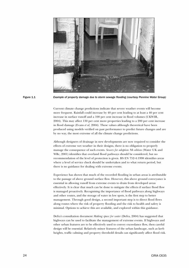
Figure 1.1 Example of property damage due to storm sewage flooding (courtesy Pennine Water Group)

Current climate change predictions indicate that severe weather events will become

more frequent. Rainfall could increase by 40 per cent leading to at least a 40 per cent

increase in surface runoff and a 100 per cent increase in flood volumes (UKWIR,

2004). This may affect 130 per cent more properties leading to a 200 per cent increase

in flood damage (Evans et al, 2004). These values although theoretical have been

produced using models verified on past performance to predict future changes and are

by no way, the most extreme of all the climate change predictions.

Although designers of drainage in new developments are now required to consider the

effects of extreme wet weather in their designs, there is no obligation to properly

manage the consequence of such events. Sewers for adoption 5th edition (Water UK and

WRc, 2001) identifies that overland flood pathways should be considered, but no

recommendation of the level of protection is given. BS EN 752-4:1998 identifies areas

where a level of service check should be undertaken and to what return period, but

there is no guidance for dealing with extreme events.

Experience has shown that much of the recorded flooding in urban areas is attributable

to the passage of above ground surface flow. However, this above ground conveyance is

essential in allowing runoff from extreme events to drain from developed areas

effectively. It is clear that much can be done to mitigate the effects if surface flood flow

is managed proactively. Recognising the importance of flood pathways along highways

and other routes, and the storage of water in low spots, is the first step to better

management. Through good design, a second important step is to direct flood flows

along routes where the risk of property flooding and the risk to health and safety is

minimal. Options to achieve this are available, and explored within this guidance.

Defra’s consultation document Making space for water (Defra, 2004) has suggested that

highways can be used to facilitate the management of extreme events. If highways and

other urban features are to be effectively used to convey exceedance flow, then careful

design will be essential. Relatively minor features of the urban landscape, such as kerb

heights, traffic calming and property threshold details can significantly affect flood risk.

CIRIA C63524

Engaging stakeholders to collectively manage and maintain flood routes, and designing

buildings to be more flood resistant, is another important factor in the equation. The

Building Regulations (2000) do not take into account property flooding and flood

resistance however in Approved Document C (HM Government, 2004), which came

into force in December 2004, provides advice on flood risk. It states that “…when local

considerations necessitate building in flood prone areas the buildings can be constructed to mitigate

some effects of flooding…”

A greater understanding of the mechanisms of drainage in extreme events and

improved guidance on how above-ground flood pathways can be effectively managed

can assist in reducing the risk of urban flooding. This guidance aims to address these

issues.

CIRIA C635 25

CIRIA C63526

Part A Overview

2 The process of exceedance and

definitions

Traditionally, urban drainage systems are designed to meet a particular and specified

level of service, known as the target level. This is normally expressed as a frequency of

property flooding. A level of protection of one in 100 years (annual probability of 0.01

being equalled or exceeded) might be defined for internal property flooding as a

suitable target for a new development. This can be delivered using a conventional

below ground piped drainage system, designed to a pipe full capacity using a one in

two year return period rainfall (annual probability of 0.5 being equalled or exceeded),

and then checking the performance for flood protection using a suitable sewer

simulation tool. Alternatively SuDS (sustainable urban drainage system) might be

specified. Its performance may be checked in a similar way. Following such checks, the

design may be amended to ensure that the desired level of protection is achieved across

the drainage area.

Existing drainage systems typically do not achieve the same level of service as that

required for new systems. This is in part due to the structural deterioration and

siltation of the existing network. More often, it is due to the network carrying increased

flows from expanding urban areas. Once system performance falls below an acceptable

level, known as the trigger level, early rehabilitation will be planned. This will then

raise system performance to an agreed target level. The performance target of a

rehabilitated system will of course be higher than the trigger level, but may be less than

the performance level for a new system. Further information on performance levels is

given in Table 3.1.

The formal or designed drainage system (piped or SuDS) is referred to in this guidance

as the minor system (Figure 2.1). For a piped system, the conveyance capacity will

normally be greater than the pipe full capacity, since additional conveyance can be

generated as flow backs up in manholes causing surcharging. The resulting slope of the

hydraulic gradient can be greater than the gradient of the pipes themselves, forcing

more flow through the system. A similar effect can occur with SuDS.

Figure 2.1 Interaction between the minor and major system during an extreme event

CIRIA C63528

Once the conveyance capacity of the minor system is exceeded, surface flooding will

occur. The excess flow that appears on the surface is known as the exceedance flow.

The rainfall events that result in exceedance flow are known as extreme events.

Exceedance flow will be conveyed on the ground by surface flood pathways. These

may be roads, paths or depressions in the surface (Figure 2.2). Where they have not

been specifically designed as flood pathways, they are known as default pathways.

Otherwise they are know as designed pathways. The system of above ground flood

pathways, including both open and culverted watercourses, is known as the major

system.

Even within the target level of service, often there will be some above ground flood

flow. Equally, there can be flooding of property before the capacity of the minor system

is exceeded. This may occur when the level of property is below the level of the

hydraulic gradient in the drainage pipes, especially where there is a direct drainage

connection. The connection between the minor and major systems is extremely

complex and can only be properly represented by a computer simulation model of

both systems. Even then, current capability of modelling above ground flood pathways

is limited. A simplified graphical representation of the interaction between the minor

and major system is given in Figure 2.3.

Figure 2.2 Conveyance of exceedance flow in surface flood pathways (courtesy Pennine Water Group)

The magnitude of surface flooding and the exceedance flow will depend on the return

period of the extreme event and the capacity of the minor system. Assuming that the

latter is equivalent to the runoff from a 10 year return period storm, Figure 2.4

illustrates typical relative magnitudes for different return periods.

It can be seen from Figure 2.4 (based upon data from a real catchment) that the

increase in runoff is by no means proportional to the increase in return period. For

example the 100 year runoff is only 1.54 × the 10 year amount. Additionally for the

100 year event, the exceedance flow to be conveyed by the major system is only 1.24

m³/s compared with the minor system flow (capacity) of 2.34 m³/s. The minor system

capacity is the difference between the exceedance flow of 0 m³/s and the runoff at

CIRIA C635 29

approximately the 10 year return period, assuming that all the runoff is drained to the

minor system. However, existing sewerage systems rarely convey the full 30 year flow

without some surface flooding, so that the surface conveyance can be expected to be

greater than this.

Figure 2.3 Simplified representation of minor/major system flow

Figure 2.4 Runoff and exceedance flow for different return period events

CIRIA C63530

3 Stakeholder roles and drainage

performance

3.1 Drainage stakeholders

The ultimate stakeholder of any drainage system is the public. Drainage provides for

an essential quality of life and effective drainage is known to be a major contributor to

the high levels of public health enjoyed by the developed world. For this reason,

effective drainage of wastewater and adequate protection against flooding are

prerequisites for both domestic dwellings and industrial and commercial property.

Property that frequently floods for example commands a lower value in the market

place. Effective drainage is important to property developers, investors and insurers as

well as the general public.

In the UK responsibility for drainage is divided between a number of organisations.

Sewerage undertakers are responsible for the public sewerage system that serves most

urban areas and some rural areas. In England and Wales, the sewerage undertaker is

the local water company, in Scotland it is Scottish Water, and in Northern Ireland this

function is delivered by the Department for the Environment (NI). Their responsibility

extends to the effectual drainage of flow arising from the land within the curtilage of

property. Recent English case law (Marcic, 2003) has shown that effectual drainage

would not be defined without limit, and that sewerage undertakers may set a

reasonable level of service that allows it to fairly distribute its investment in improving

sewerage infrastructure to the most needy areas. Sewerage undertakers will define a

target level of service, this typically being protection against flooding from storm flows

arising from a 30 year return period event. Priority will be given to cases where

flooding occurs more frequently, the trigger for early rehabilitation being set typically

at a one in 10 year frequency level.

The responsibility for the maintenance of minor watercourses in rural and urban areas

falls to riparian owners and the local drainage authority. Local authorities may be

unitary or, for example, district or borough councils as part of a two-tier system. For

ordinary water courses in England and Wales this lies with the local drainage board or

local authority. For statutory main rivers the function lies with the Environment

Agency. Similar mechanisms exist in Scotland and Northern Ireland. Highway drainage

is normally the responsibility of the local highway authority. Under a non-statutory

agreement, highway drains may discharge into public sewers and vice versa.

The responsibility for drainage is fragmented which makes management more complex.

Property owners are responsible for drainage within the curtilage of their property. They

are also responsible for insuring their property against flooding. Historically, insurers have

provided insurance for flooding (including flooding caused by the limiting capacities of the

minor system in extreme events) for all properties at the same levels of premium. This is

now changing because of the increased incidence of flooding in recent years, caused by

climate change. Insurers are gradually introducing risk based premiums for flooding.

They have advised that protection from a one in 200 year return period event (annual

probability of flooding of 0.005 being equalled or exceeded) is the minimum standard at

which flood insurance is likely to be available at what most would regard as normal

premiums. Where the risk is greater than one in 75 years (annual probability of 0.013

CIRIA C635 31

being equalled or exceeded), insurance may not be readily available for new business and

could be considered very expensive. A gap has opened between the level of service that

sewerage undertakers aim to provide and the minimum standard of protection that

insurers consider necessary to provide cover that is affordable.

As explained earlier in the previous chapter, effective management of the runoff from

extreme events is a growing consideration. Achieving this will require the co-operation

of the relevant stakeholders, these being the sewerage undertakers, highway

authorities, local authorities, Environment Agency/DOE (NI)/SEPA, property owners

and insurers. For new developments the role of the developer and the planning

authority will also be important. Further information can be found in PPG25

Development and flood risk (DTLR, 2001) and CIRIA C624 Development and flood risk –

guidance for the construction industry (Lancaster et al, 2004).

3.2 Managing extreme events in existing urban areas

One of the most challenging aspects of managing the effects of extreme events in

existing urban areas is the division of responsibility for drainage set out above. The

general public do not understand (and do not wish to understand) the technicalities of

current legislation. Government has indicated that urban drainage responsibilities may

need to be reviewed (Defra, 2004) however a pragmatic way forward needs to be found

in the interim.

In cases of actual flooding of property it is all too easy for one body to attempt to pass

the blame onto another. When flooding occurs it is usually difficult to be precise about

the return period of the event, whether or not flood water has originated from land

outside of a curtilage or from the highway, or if local watercourse flooding has

contributed.

The delivery of timely and robust solutions to urban flooding requires the effective co-

operation of the various stakeholders. Further guidance on managing stakeholder

interaction is given in Part B, Chapter 5.

3.3 The role of the planner and developer in new developments

Where new developments are proposed, the ability to effectively drain the site is very

important and should be a concern for both the planner and the developer. From the

developer’s perspective, effective drainage (in terms of the minor and major system) is

essential in order to deliver maximum value from investment as the inability to gain

flood insurance on normal terms can significantly affect property values. The planner’s

role is important, not only to ensure that the proposed development can be effectively

drained above and below ground, but also that there are no significant consequential

effects downstream.

Planning applications have to be determined in accordance with the provisions of the

“development plan”. There is a requirement for planners to consult the various bodies

responsible for drainage such as the Environment Agency, sewerage undertaker and

local authorities drainage engineers including highways. Further information is given

in Chapter 5 and in X108 Drainage of development sites – a guide (Kellagher, 2004).

Developers need to consider site drainage early in the development process, and

certainly no later than the stage of land acquisition, since drainage can affect land

value. The layout of a site can have a substantial impact on the ability to cost-effectively

CIRIA C63532

manage extreme events in the developed area (see Part B, Chapter 13). Designers

should consult responsible bodies at an early stage before submission of the planning

application (whether outline or full) and this would greatly assist planners in reaching

their decisions. This should be considered in detail by both developers and planners.

3.4 Drainage design and performance standards

It is apparent from the above that different stakeholders are responsible not only for

different drainage systems but also for different levels of performance of the same

system. There are numerous design guides that cover drainage design and recommend

appropriate standards. These standards often overlap and this can cause considerable

confusion with stakeholders. To help clarify some of these issues, Table 3.1 highlights

the main drainage performance standards and indicates where appropriate the

relevant responsible body.

At present there are no guidelines on the return period of event (extreme event) that

should be used for designing for exceedance. It is suggested that return periods of one

in 30 to one in 100 or one in 200 year events would form a suitable framework for

most applications. Where health and safety issues are important it could be argued that

the concept of “any conceivable event” inherent in the procedures set out in the

Reservoirs Act 1975 might be applicable. For this purpose the 1000 year event may be

suitable. Further guidance on design criteria is given in Chapter 11.

3.5 Key stakeholder lessons

The development of sustainable solutions to exceedance flooding will only be fully

realised through good stakeholder interaction. At the start of any project, stakeholders

should identify who is responsible for the flooding (which maybe a number of parties)

and establish who has an interest in its resolution. The problem should be clearly

defined and communicated to all parties. Flood liaison and advice groups (FLAGS see

Section 5.8) have been shown to be one way of effectively achieving this. The limits

within which various stakeholders operate should be clearly defined so that their

expectations are managed effectively (Ashley et al, 2005).

CIRIA C635 33

Table 3.1 Drainage design and performance standards

CIRIA C63534

Return

Period

(1 in n

years)

Description of hydraulic performance

Ge

ne

ral

de

sig

n

pri

nc

iple

s

Are

a f

loo

din

g

cri

teri

a

Pro

pe

rty

flo

od

ing

cri

teri

a

Code of practice or

standard

1

Pipes designed to run just full – sites with

average ground slopes greater than one

per cent×

Sewers for adoption

5th edition

1 Surface water highway design ×

Design manual for

roads and bridges

4th edition

1-2 Council highway drainage design × Council dependant

2Pipes designed to run just full – sites with

average ground slopes less than one per cent×

Sewers for adoption

5th edition

2 Design of highway sewers × Council dependant

5

Where there are consequences of severe

flooding (eg near basements) – pipes

designed to not surcharge×

Sewers for adoption

5th edition

5 No flooding of highway sewers × × Highway Agency

5 Design of channel drainage in highway × Highway Agency

10 Protection of rural areas from flooding × BS EN 752 Part 4

20Current Ofwat reporting level for internal

and external flooding× × Ofwat

20Protection of residential areas from

flooding× BS EN 752 Part 4

30

No flooding in any part of the residential

area×

Sewers for adoption

5th edition

Protection of city centre/commercial areas

from flooding× BS EN 752 Part 4

Level of service for no flooding for existing

systems×

Typical water

company criteria eg

Yorkshire Water,

Scottish Water and

Southern Water

50Protection of underground railways and

underpasses× BS EN 752 Part 4

50No flooding from the minor drainage

system for new sewers×

ABI lobbying through

response to Making

Space for Water

75 General level of protection from flooding ×

ABI – Statement of

Principles on the

Provision of Flooding

Insurance

100

Guidelines for new developments where all

flows are retained on site (with an

allowance for climate change [+20 per

cent] which is greater than 1 in 200 year

× EA guidance

100No flooding from the minor drainage

system×

Typical insurance

company lobbying eg

Norwich Union

50-

200Protection from river flooding Unclear

MAFF 99 (from

PPG25)

200

Minimum level of protection for residential

properties for flooding giving “normal terms

of cover”×

Statement of intent

by ABI

100-

333Protection from coastal flooding Unclear

MAFF 99 (from

PPG25)

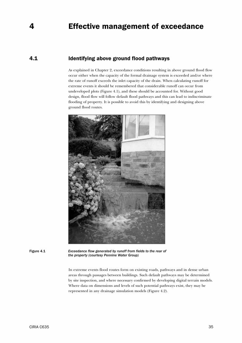
4 Effective management of exceedance

4.1 Identifying above ground flood pathways

As explained in Chapter 2, exceedance conditions resulting in above ground flood flow

occur either when the capacity of the formal drainage system is exceeded and/or where

the rate of runoff exceeds the inlet capacity of the drain. When calculating runoff for

extreme events it should be remembered that considerable runoff can occur from

undeveloped plots (Figure 4.1), and these should be accounted for. Without good

design, flood flow will follow default flood pathways and this can lead to indiscriminate

flooding of property. It is possible to avoid this by identifying and designing above

ground flood routes.

Figure 4.1 Exceedance flow generated by runoff from fields to the rear ofthe property (courtesy Pennine Water Group)

In extreme events flood routes form on existing roads, pathways and in dense urban

areas through passages between buildings. Such default pathways may be determined

by site inspection, and where necessary confirmed by developing digital terrain models.

Where data on dimensions and levels of such potential pathways exist, they may be

represented in any drainage simulation models (Figure 4.2).

CIRIA C635 35

Figure 4.2 Above ground flood pathways identified during a site development study. Different shadedarrows refer to different types of above ground pathway (courtesy Glasgow City Council)

4.2 The capacity of surface pathways

The capacity of drainage pathways may be determined by hand calculation. However,

by far the better method is to represent them in drainage simulation models. Modern

computer models readily allow modelling of such pathways by representing them

through open channels. Further information on this is given in Sections 11.3 and 11.4.

If property flooding is to be avoided, then the conveyance capacity of flood pathways

should be designed so as to convey the whole of the exceedance flow (design pathways).

The conveyance capacity can be significantly influenced by relatively minor detail such

as kerb heights. Often the effective conveyance of flood flow can be achieved by

modifying the detail of a carriageway cross-section, for example by revising the detail of

drop kerbs.

Surface pathways should be linked together in the same way as conventional drainage

networks, so as to provide a system of conduits that effectively conveys the exceedance

flows off the developed site. Flows should be prevented from accumulating at low spots

except where temporary surface storage is incorporated into the design strategy

(Figure 4.3).

When designing surface flood pathways the designer should remember that unlike

conventional drainage they will only convey significant flow very rarely. In practice they

will be used on a day to day basis for other purposes. For example, a grass lined

channel may be used to convey exceedance flow across an area of open space. The

channel will normally be used for recreational purposes and the designer needs to

consider the implications of this. For example:

CIRIA C63536

� what safeguards will be in place for its continued availability as a flood channel? Its

use for this might be compromised if a fence were to be constructed across its path.

� when the channel is in use for flood conveyance, the public may suddenly be

exposed to unexpected flow depths and velocities. What criteria will be used to

limit depth and velocity in order to protect public safety?

� after the event, what measures will be in place to clear out any sediment, litter or

polluting material? How will the public be warned about the potential hazards of a

flood pathway in their community?

Further details on the design and management of surface channels may be found in

Chapter 11.

Figure 4.3 Unplanned ponding of surface flood flow at a low spot leading to property flooding (courtesyPennine Water Group)

4.3 Providing surface storage

When providing effective surface flood pathways for extreme events in existing urban

areas one of the challenges faced is that the space may not be available to achieve the

required conveyance capacity. Where full surface conveyance capacity cannot

economically be provided, reduced capacity may be accommodated if flows can be

attenuated on site. This can be achieved by the planned provision of surface storage.

As with surface flood channels, surface storage can be accommodated using areas that

are used for other purposes for most of the time. When considering potential areas the

following questions should be answered:

1 What depth of storage would be necessary to achieve the required flooding

volume?

2 How long will it take for the area to drain after the event?

3 How will the temporary storage of flood volume affect the primary use of the area?

CIRIA C635 37

4 Will any damage or important loss of use occur?

5 Will standing water create an unacceptable risk to public health or safety?

Storage on an existing car park to a moderate depth less than kerb height might be

acceptable. Structural damage is likely to be insignificant, and if only surface runoff is

being stored, then health and safety risks are likely to be acceptable. There will be some

loss of use, but provided the area drains relatively quickly after the event, this should

not be a problem in most situations.

The required storage volume can in many cases be large. This is especially true where

storage is being used to mitigate the impacts of exceedance flow conveyance to

downstream systems (see Section 4.4 and Chapter 14). The designer should consider

the potential of sacrificial areas in such cases. These are areas of low value land to

which exceedance flood volumes can be discharged and retained for longer periods of

time. Such areas may not have identified outfalls with the water stored infiltrating slowly

into the ground and/or evaporating over a period of time after the event.

4.4 The effect of building layout

The spatial distribution of buildings on a site can greatly influence the potential for

creating flood pathways and considerably affect property flood risk. Little can be done

to affect the building layout in existing urban areas except where significant

redevelopment is anticipated. However, much can be done to manage cost effectively

exceedance flows in new developments by careful layout of buildings (see Chapter 13).

In any new development it is important that the drainage of the site, including extreme

events, is considered at the earliest possible date. Ideally its effects should be part of

initial negotiations for land acquisition as it may significantly affect land value. Flood

flow paths should be considered in the light of the natural drainage pathways on the

site, and space left between buildings to accommodate them. Where roads and

pathways can be arranged to act in a secondary capacity as flood pathways then the

management of exceedance flows will be much easier. Further details are provided in

Chapter 13.

In particular designers and developers should be wary of locating high value property

such as housing at low spots, as floodwater will always tend to accumulate there. If

unavoidable, special care should be taken to ensure that such property is protected

from accumulated flood volumes by raising threshold levels, and/or providing

additional drainage.

In many cases it may be more cost effective to amend site layout and the above ground

flood channels (major system) rather than alter the below ground (minor) drainage system.

4.5 Impact on downstream systems

The rapid transfer of exceedance flow over the surface can have a significant and

damaging impact on downstream receptor systems. The situation is exacerbated when

such systems themselves are subjected locally to the effects of an extreme event at the

same time, and this can impose significant additional liabilities on stakeholders.

Advice on assessing the impact on downstream systems and developing mitigation

measures is given in Chapter 14. However a few vital points are worth noting.

CIRIA C63538

It is important to understand the dynamic interaction between the upstream system

conveying the flow, and the downstream receptor system. As well as considering the

peak rate of runoff and the flood volume, the timing of the peak relative to that in the

receptor system is essential. For example, where a small upstream area discharges into

a large river system, the actual impact may be small, not because the rate of exceedance

flow is small, but because the maximum value occurs ahead of the peak in the receiving

river. It may pass downstream without detriment and in such cases it may be

detrimental to provide storage attenuation if this leads to the peak flows occurring at

around the same time.

The downstream system can also prevent the exceedance flow from freely discharging,

increasing the risk of upstream flooding. For example, when discharging to coastal

areas, tide levels may affect the performance of surface flood pathways. An extreme

event coinciding with a high tide may not drain as effectively as one occurring at the

time of a low tide. In such cases a joint probability analysis may be necessary.

Outfalls from surface flood pathways may require agreements/consents from the

owners of receiving watercourse, riparian owners and/or environmental regulators.

Early planning of such consents or agreements will greatly assist in land

(re)development.

Exceedance flows may convey large quantities of sediments, pollutants washed of

surface areas, and other pollutants discharged from wastewater collection systems.

These may also have a significant impact on receptor systems, however their

consideration is beyond the scope of this guidance.

4.6 Post-event clean-up

Any exceedance event may leave debris or even pollution in storage areas and overland

flow paths. In such designated areas procedures for a timely clean-up operation by the

responsible stakeholder should be agreed. This may require the removal of debris and

pollution, and the spraying down/disinfection of areas where combined sewage flooding

has occurred.

CIRIA C635 39

CIRIA C63540

Part B Detailed design

5 Managing stakeholder interaction

5.1 The planning process

It will be apparent from the previous section that exceedance flows generated from

extreme events will be conveyed on the surface of the flood pathways. Surface storage

for these may also be provided. The ability to manage such flows effectively, so as to

minimise a sudden increase in flow, will depend on topography, building layout and the

configuration of other infrastructure, especially highways. Consideration of site

drainage early in the planning process is essential.

Sewers for adoption 5th edition (Water UK and WRc, 2001) contains guidance on the

means of effectively draining a site, this includes a requirement to consider drainage of

flows and overland flow routes from extreme events. Planning applications should

explicitly refer to the drainage of exceedance flows. As stated above, and elaborated in

later chapters, the provision of effective surface flow pathways and storage areas may

have a significant impact on highway design, building layout, and the provision of

other infrastructure. It is essential that consultation with the stakeholders responsible

for this infrastructure takes place early in the planning process, and certainly before a

formal application for planning permission is submitted.

For new developments, consideration should be given to the existing natural drainage

of the site, as explained in Chapter 6. Wherever possible, surface flow pathways and

storage areas should take account of the natural topography and land form, and should

be included in the framework of the development. Further information on this given in

Chapters 12 and 13.

The general principles of the town and country planning systems in the four home

countries (England, Scotland, Wales and Northern Ireland) are broadly the same. They

all have both strategic and local development plans guiding the location and form of

development, and powers by which local planning authorities can control detail in

granting planning permission for individual developments. However there always have

been differences and divergence has tended to increase since devolution in the late

1990s.

The system described below is that operating in England since the Planning and

Compulsory Purchase Act came into effect at the end of September 2004. Details of the

arrangements in Scotland, Wales and Northern Ireland are available on the respective

websites: <www.scotland.gov.uk>, <www.wales.gov.uk>, and <www.drdni.gov.uk>. A

planning bill, introducing significant change, is expected in the current session of the

Scottish Parliament, 2005.

The planning process involves applying for planning permission to the relevant local

planning authority and can be in outline or detail. An outline application is

recommended where it is necessary to establish matters of principle in connection with

a large or complex development before proceeding to detailed design.

Under the “plan led” system, introduced by the Planning and Compensation Act 1991,

and now embodied in the Planning and Compulsory Purchase Act 2004, local planning

authorities are required to determine planning applications in accordance with the

CIRIA C63542

CIRIA C635 43

provisions of the development plan, unless material considerations dictate otherwise.

This gives the “development plan”, and the policies and proposals it contains, a

particular significance.

The statutory development plan is now composed of two main elements:

� the Regional Spatial Strategy (RSS), prepared by the regional planning body for

each English region

� the Local Development Framework (LDF) – a folder containing a range of

planning documents, prepared and adopted by each district and unitary authority.

The new plans, at both regional and local levels, are “spatial” plans. This means that

they can be much more integrative and inclusive than the old style plans that were

confined to a narrower land use planning remit. As a result, management issues such as

flood management for example are now a legitimate concern of development plans.

The more detailed, lower order plans that make up the LDF ought to be in general

conformity with the regional spatial strategy. So it is important for stakeholders to make

representations during the plan preparation process so that the RSS can contain the

right strategic policies to guide more detailed, local policies and proposals. For example

it might be appropriate to specify in the RSS that all new development should adopt

the principles of sustainable drainage.

Applicants for planning permission need to be aware of the details contained in the

development plan, not only about development in specific locations, but also in any

generic policies – about requirements for flood management or sustainable drainage,

for instance – that cover the whole plan area. Equally, “statutory consultees”, such as

the Environment Agency, have the facility to ensure that appropriate policies, covering

their area of interest, are included in the plan. Stakeholders who are not included in

the list of consultees in Annex E of PPS12 Local development frameworks (CLG, 2004a)

should still have the opportunity to make a contribution to the plan making process.

There is now a statutory requirement for local planning authorities to give greater

weight to stakeholder consultation and community involvement.

5.2 Stakeholder responsibilities

In the UK, currently there is no single body responsible for urban drainage and flood

control. However Defra’s consultation document, Making space for water (Defra, 2004),

which is applicable to England only, suggests a number of alternative options for the

management of surface water.

The delivery of effective drainage involves many organisations and is covered by

statute, formal and informal agreements. The process is complex, even more so where

above ground flows are concerned. To complicate matters further, legislation and

agreements in Wales, Scotland and Northern Ireland are different from England. The

main stakeholders relevant to drainage are summarised in Table 5.1 and discussed

further in this chapter.

Figure 5.1 Recommended good practice for managing drainage in the development process (adaptedfrom Woods-Ballard et al, 2007)

CIRIA C63544

Master plan for large

scale developments

Outline planning

permission

Stakeholder

consultation

Long-term

maintenance

agreement

Outline

drainage

Land purchase (before

or after planning

permission)

Detailed data

and modelling

Drainage design

(including major and

minor system), drainage

impact assessment

Initial stakeholder

consultation

Initial data/

characteristicsDevelopment concept

Develop initial

drainage concept

Input ProcessKey:

� planning permission

� Building Regulations approval

� drainage construction consent

� road construction consent

� consent to discharge.

Output

Table 5.1 Stakeholders responsible for drainage in England and Wales (after NSWG, 2004)

5.2.1 Local authorities

Local authorities have a large number of responsibilities including:

� planning

� building control

� local roads

� public landscaping

� highway drainage

� land drainage

� welfare.

There are two systems of local authorities in England, either unitary or two-tier. Their

responsibilities are either split or joint. Under a unitary authority the drainage and

highway departments will be under one body with the planners. However in a two-tier

system, highways are under the control of the county council whereas the detailed

planning issues and drainage are the responsibility of the district or borough council.

The local authority building control department (or an accredited private organisation)

is responsible for ensuring through their inspectors that the Building Regulations have

CIRIA C635 45

Name Function Authority

Local authority

drainage

departments

Drainage, flood alleviation and

regulation of watercourses, apart from

designated main rivers.

Particular responsibilities in

drainage districts. Set out in the

Land Drainage Act 1991.

Highway authorities Responsibility to keep the roads

(except trunk roads) free from flooding

and to make provision for runoff from

highways in a proper manner.

Relevant legislation includes the

Highways Act 1980 and the Land

Drainage Acts 1991 and 1994.

Internal drainage

boards

Supervisory duty over flood defence

and drainage for low-lying land in

England and Wales.

Regulation of watercourses apart from

designated main rivers within

specified areas.

Set out in the Land Drainage Acts

1991 and 1994, covering

maintenance, improvement and

operation of drainage systems,

conservation and revenue-raising.

Sewerage

undertakers

Responsibility for maintaining a public

sewerage system, which includes

sewers carrying surface water away

from impermeable areas.

Set out in the Water Industry Act

1991 and 1999, which obliges

sewerage undertakers to provide

and maintain a drainage and

sewerage system, and to authorise

and charge for the discharge of

trade effluent to sewers. Highly

regulated by Ofwat.

Environment Agency The Agency aims to protect and

enhance the environment and to

make a positive contribution towards

sustainable development in England

and Wales. Its water management

functions include:

� water resources regulation and

planning

� water quality regulation and

planning

� flood defence and drainage,

maintenance and operations in

statutory main rivers.

Powers and duties set out under the

Environment Act 1995 and related

legislation. Regulation and executive

action on water resources, land,

water and air quality, flood and

coastal defence, flood warning,

waste management, navigation,

conservation, fisheries and

recreation.

been adhered to. An important role for the inspectors is to be satisfied with the level of

drainage provided and that it does not affect the integrity of the property (this could

include above ground pathways).

The local authority planning departments are responsible for approving new

development that includes drainage and can influence the adoption of SuDS and the

introduction of above ground pathways. CIRIA C625 Model agreements for sustainable

water management systems (Shaffer et al, 2004) sets in place a process to enable SuDS

systems to be adopted. The funding for ongoing maintenance can be provided through

commuted sums (paid by the developer) or through a bond (Shaffer et al, 2004).

Highways authorities

The responsibility for the drainage of highways falls to the local highway authority. This

will usually be the unitary authority or the county council. Highway drainage may be

connected to sewerage and vice versa under a generic non-statutory agreement

between sewerage undertakers and highway authorities. Highway authorities are not

responsible for the trunk road network. This is the responsibility of the Highways

Agency in England, the Transport Directorate in Wales, the Roads Service in Northern

Ireland and the Scottish Executive in Scotland.

Land drainage authorities

Land drainage is the responsibility of the local land drainage authority who have

permissive powers and are normally the local authority, local land drainage board or

county council. For most areas this responsibility lies with the Environment Agency

(England and Wales), SEPA (Scotland) and the DOE (Northern Ireland). However in

Scotland the local authorities are responsible for the ‘primary flood management’ so

understanding the rate and volume of surface water runoff from any new development

is important.

5.2.2 Sewerage undertakers

In England and Wales, the sewerage undertaker is responsible for ensuring the

effective drainage of developed areas (Water Act 1989 and Water Industry Act 1991).

However, this responsibility is limited to runoff from areas that are within the curtilage

of individual properties. The adoption of sewers is generally constrained to adopting

piped systems with proper outfalls and can be legally defined as a “sewer” (NSWG,

2004). It does not include the drainage of any highway or undeveloped area, or

general land drainage. Views differ as to whether or not a sewerage undertaker has a

duty to drain large undeveloped areas within a property curtilage.

The drainage responsibility is normally delivered through the provision of a sewerage

system, and a sewerage undertaker is obliged to adopt such systems provided that

certain conditions are met. In England, Wales and Northern Ireland, there is a

statutory definition of a sewer that specifies its conveyance function but does not restrict

it to being a pipe. However the definition does not extend to include surface storage

provision. Legislation in Scotland allows for the inclusion of surface storage in order to

facilitate sewerage undertakers development. Sewerage undertakers may require a

licence to discharge to receiving water (British Waterways Board v Severn Trent Water

Plc, Court of Appeal, 2001) and may also require a consent for the outfall structure.

The drainage responsibility of sewerage undertakers does not extend to any

conceivable event, but is restricted to exclude extreme events. As set out in the Marcic

Appeal ruling (Court of Appeal, 2002), this is in recognition that sewerage undertakers

CIRIA C63546

have limited powers to raise charges and limited obligations, although there is a

requirement for them to set level of service standards as a means of prioritising that

investment. Sewerage may be separate (separate pipes for surface water and foul

sewage) or combined. A landowner has the right to connect to a public sewer, though

where a separate system is provided, this has to be the appropriate sewer. The sewerage

undertaker may specify the point of connection.

Within the curtilage, drainage is the responsibility of the land owner. However existing

developments may fall under Section 179 of the Water Industry Act 1991 where sewers

built before 1 October 1937 are the responsibility of the undertaker. This does not

prevent a sewerage undertaker making provision for flood protection within the

curtilage, say by providing reasonable flood barriers, but there is no statutory

obligation for them to do this, and it would have to be with the agreement of the land

owner. Landowners also have the responsibility for insuring against flood risk, although

the ability to secure such insurance may be influenced by factors outside their control.

5.2.3 Environmental regulators

In England and Wales the Environment Agency (EA) has a wide range of

responsibilities, of which the key ones are described in Table 5.1. It can exercise powers

to deal with flooding, however, it has no liability relating to it. It is directly responsible

for performance and maintenance of main rivers and critical ordinary water courses

(where they have been designated as main). The EA may operate and provide flood

warning systems (Section 166 of the Water Resources Act 1991).

The EA is a statutory consultee for specified activities as set out in the Town and

Country Planning (General Development Procedure) Order 1995. However, it is not a

statutory consultee for all drainage related applications requiring a consent to discharge

to a watercourse. It will offer guidance to the planning authority on the rate and

volume of surface runoff from new developments. In Scotland this is undertaken by the

local authority and in Northern Ireland by the Rivers Agency. Other responsibilities in

these areas lie with the Scottish Environmental Protection Agency and the Northern

Ireland Environment and Heritage Services.

The EA has the powers to serve conditional prohibition notices related to the quality of the

water but not to dictate the standards of how a drainage system should be constructed.

5.3 Stakeholder consultation process

5.3.1 Initial stakeholder consultation phase

The process of reaching early stakeholder agreement is achieved by undertaking the

following points:

� identifying criteria for drainage design

� understanding individual stakeholder responsibilities and requirements

� understanding the impact on local communities

� early and regular consultation

� the building of effective personal relationships and trust

� including drainage costs when the site is purchased.

The drainage stakeholders described in Section 5.2 and local authority planners should

be consulted during the initial stakeholder consultation phase. During this phase

CIRIA C635 47

stakeholders should be made aware of and contribute to further developing the surface

water network and drainage criteria. This should include proposals to manage

exceedance through above ground conveyance and storage if required.

Information collected at this stage of the planning process should enable the planning

authority to identify if further details of site drainage are required. This may be through

a drainage impact assessment using tools described in this publication for the exceedance

element where necessary prior to the submission of a planning application. In addition it

may be prudent to consult other stakeholders with interests around the development site.

A drainage impact assessment may be used to demonstrate how surface water will be

drained and identify the principles for controlling exceedance flows from extreme

events. This will enable the planning authority to set conditions to manage flooding

during extreme events.

5.3.2 Stakeholder consultation phase

The main stakeholder consultation phase will require outline drainage design to be

submitted which should include the above ground conveyance and/or storage locations

if deemed necessary. A risk assessment of the area should be undertaken to determine

levels of service and risk of flooding using this guidance. A flood risk assessment may be

required depending upon the planning policy in England (PPG25), Wales (TAN15),

Scotland (SPP7) and Northern Ireland (PPS15). A drainage impact assessment should

be included in any flood risk assessment.

It is critical during this phase that the developer and their drainage designer should

liaise with the regulatory authorities to agree the appropriate criteria. In particular, the

standards and protection to flooding should be confirmed to ensure the risks are

adequately designed and managed. A general summary for drainage design is provided

in CIRIA’s drainage and SuDS guidance. In areas where changes are being made to

existing drainage infrastructure to facilitate the improved management of drainage

exceedance, it will be necessary to consult and liaise with a wider range of stakeholders,

including existing residents and commercial businesses.

5.4 Good practice in stakeholder interaction

Good practice in stakeholder interaction requires a well planned and open process.

Completing a drainage impact assessment (North East Scotland Flooding Advisory

Group, 2002) helps to understand and manage the impacts of a proposed

development. In Scotland, local authorities are beginning to request this assessment

and this method. In conjunction with the guidance it will ensure that above ground

pathways are considered, designed and actively managed (NSWG, 2004). The EA in

England and Wales have provided guidance for flood risk assessments

<www.environment-agency.gov.uk/research/planning/33098.aspx> depending upon

location within flood zones which includes the assessment of surface water impacts and

exceedance.

There is little current experience in stakeholder collaboration in achieving designed

surface flood conveyance and storage systems for managing extreme events. However,

examples of good practice can be drawn from stakeholder collaboration to reach

solutions of other flooding problems where responsibilities are shared. Three examples

of good practice follow in Sections 5.4.1, 5.4.2 and 5.4.3.

CIRIA C63548

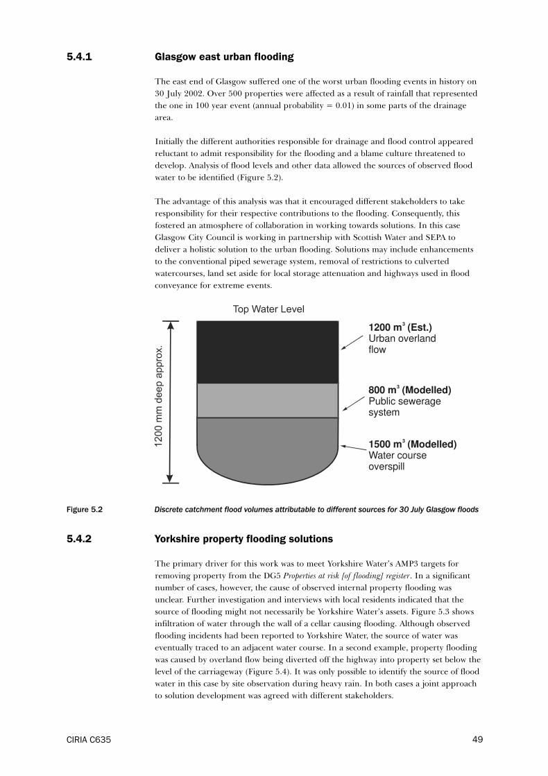
5.4.1 Glasgow east urban flooding

The east end of Glasgow suffered one of the worst urban flooding events in history on

30 July 2002. Over 500 properties were affected as a result of rainfall that represented

the one in 100 year event (annual probability = 0.01) in some parts of the drainage

area.

Initially the different authorities responsible for drainage and flood control appeared

reluctant to admit responsibility for the flooding and a blame culture threatened to

develop. Analysis of flood levels and other data allowed the sources of observed flood

water to be identified (Figure 5.2).

The advantage of this analysis was that it encouraged different stakeholders to take

responsibility for their respective contributions to the flooding. Consequently, this

fostered an atmosphere of collaboration in working towards solutions. In this case

Glasgow City Council is working in partnership with Scottish Water and SEPA to

deliver a holistic solution to the urban flooding. Solutions may include enhancements

to the conventional piped sewerage system, removal of restrictions to culverted

watercourses, land set aside for local storage attenuation and highways used in flood

conveyance for extreme events.

Figure 5.2 Discrete catchment flood volumes attributable to different sources for 30 July Glasgow floods

5.4.2 Yorkshire property flooding solutions

The primary driver for this work was to meet Yorkshire Water’s AMP3 targets for

removing property from the DG5 Properties at risk [of flooding] register. In a significant

number of cases, however, the cause of observed internal property flooding was

unclear. Further investigation and interviews with local residents indicated that the

source of flooding might not necessarily be Yorkshire Water’s assets. Figure 5.3 shows

infiltration of water through the wall of a cellar causing flooding. Although observed

flooding incidents had been reported to Yorkshire Water, the source of water was

eventually traced to an adjacent water course. In a second example, property flooding

was caused by overland flow being diverted off the highway into property set below the

level of the carriageway (Figure 5.4). It was only possible to identify the source of flood

water in this case by site observation during heavy rain. In both cases a joint approach

to solution development was agreed with different stakeholders.

CIRIA C635 49

1200 m (Est.)3

Urban overlandflow

800 m (Modelled)3

Public seweragesystem

1500 m (Modelled)3

Water courseoverspill

Figure 5.3 Cellar flooding from infiltration from a local watercourse

Figure 5.4 Property flooding by overland flow from the highway

CIRIA C63550

5.4.3 Flooding of residential area in Birmingham

In this case the flooding of an area of urban housing was traced to a number of sources

(O’Leary, 2004). In all, the following agencies were identified as having some

responsibility towards that flooding:

� Severn Trent Water.

� Environment Agency.

� Sandwell Council (Riparian Owners).

� Highways Agency.

� British Waterways Board.

Figure 5.5 shows the sources of and properties affected by flooding, while Figure 5.6

indicates the overland flow routes. An agreed scheme was developed where different

sub-schemes, each associated with a particular stakeholder, were identified. Subsequent

delivery of the sub-schemes is the responsibility of the respective stakeholder. Although

early benefits will be achieved from individual stakeholder sub-schemes, the full benefit

will only be realised when all are delivered. The process is self regulating and as the

various sub-schemes progress, the pressure on the remaining stakeholders to fulfil their

obligations increases.

Figure 5.5 Property location of flooding in a Birmingham suburb attributed to a number of sources(courtesy Seven Trent Water)

CIRIA C635 51

Figure 5.6 Plan showing overland flow paths for the flooding shown in Figure 5.5 (courtesy Seven TrentWater)

5.5 Ownership and legal rights

Traditionally as new sewerage is completed, a sewerage undertaker adopts it.

Ownership then transfers to the undertaker who is subsequently responsibly for

maintenance and periodic capital renewal, in order to assure the required level of

service. The situation is more complex with above ground conveyance and storage

systems for extreme events. There is no statutory requirement for a sewerage

undertaker to adopt since they are designed only to drain extreme events and may be

construed as being beyond the definition of “effectual” drainage. Moreover, in many

cases the drainage function will not be the primary function of the facility (see Chapter

11). A good example is where a highway is being used for the conveyance of

exceedance flows.

It is possible that the sewerage undertaker or other responsible drainage authority will

not be the owner of the facilities delivering effective flood control for extreme events.

The drainage authority’s responsibilities will have to be secured through a license

arrangement with the owner, entered into by voluntary agreement. For new

developments it would be possible to secure licence agreements by making it a

condition in the planning permission. However in retrofit scenarios securing such

agreements will be more difficult. No model agreements exist for this purpose, but the

model agreements for SuDS may form a useful starting point (Shaffer et al, 2004). The

license may include certain duties that the owner might be responsible for, such as

routine maintenance, and a responsible stakeholder may need to pay a commuted sum,

and/or indemnify the owner from liability in him exercising these duties.

CIRIA C63552

5.6 Education – the public as stakeholders

During the planning process, the general public will have very limited involvement.

However it is the general public who have to deal with the consequence of exceedance

and drainage failure as a result of flooding. Educating them to understand a new

strategic approach to managing exceedance is very important. The key areas that

should be addressed through an education programme are:

� the minor system cannot convey all flows

� flooding is ‘acceptable’ if controlled and managed

� it is not sustainable and especially cost effective to design sewers to convey flows

with a return period greater than one in 30 years (current standard in Sewers for

adoption 5th edition)

� explain the concept of return periods and probability with sewerage system design,

and the impact of climate change

� excess flows that do occur can be controlled and managed

� flows can be conveyed using a variety of above ground conveyance channels

including roads

� during periods of heavy rainfall it is advisable to not travel by foot or car along or

in urban flood pathways

� identifying areas for temporary storage will help prevent other areas being

flooded.

If these points are addressed, the general public may have a greater understanding of

the challenges that exist and how they can be managed.

5.7 Flood warning

The EA have a flood warning process that includes “monitoring weather, river and

coastal conditions, forecasting river and sea levels, disseminating flood warnings, and

influencing those at risk to take effective action to prepare for and respond to flood

warnings” (Murphy, 2003). It is possible for the EA to perform this function as it is one

body with national coverage and the drivers for fluvial flooding are slower than those

for pluvial.

It is unlikely that even if a national body existed representing the sewerage system, that

flooding in areas related to exceedance could be forecast in time to then issue a flood

warning. However, this guide promotes the use of above ground conveyance routes

and storage areas to control above ground flows. These need to be adequately signed to

warn users that during extreme events, access to the areas should be avoided or even

restricted. This is particularly important for storage areas where higher flow depths

may be experienced than in conveyance channels. A gradual transition of the build up

of flows, rather than a sudden increase, is also important, and will act as a warning to

the general public.

5.8 Stakeholder collaboration

The achievement of good exceedance design will be achieved through good

stakeholder interaction and dialogue. This should include stakeholders with drainage

interests, planners, developers, local interest groups and homeowners. However the

exact make up will depend on the location as well as whether it is an existing or new

CIRIA C635 53

54 CIRIA C635

development. The group of stakeholders should be established at the start of the

project with the objectives of each stakeholder and the boundaries of operation and

their responsibilities clearly set out.

Stakeholder interaction could be enhanced through the setting up of flood liaison and

advice groups (FLAGS) that are encouraged in PAN 69 (Scottish Government, 2004). In

Scotland their purpose is to share knowledge and act in the interest of private and

public stakeholders. FLAGS generally have an overseeing role, can cover a wide

catchment area and may meet several times per year. FLAGS could be used in a co-

ordination role over a wide area and help in the development of good relationships

between stakeholders.

6 Runoff from natural catchments

6.1 Introduction

Urban drainage has evolved over the centuries, but in recent times it has become clear

that the runoff characteristics of urban areas, both in terms of flow and water quality

impacts, can have an undesirable effect on the receiving environment. When natural

surfaces are paved, the volume and rate of runoff increases. More sediments and other

pollutants are mobilised and transported into the downstream system.

If the impact of urban drainage is to be minimised in the future, then it will need to

mimic natural drainage processes much more closely than at present. To achieve this,

engineers and practitioners will first need to understand how natural areas drain. From

this understanding, criteria for urban drainage can be developed to provide the most

appropriate system for a particular site or development:

� understanding rural or greenfield runoff is also important

� water levels in any natural watercourse that runs through a site can be estimated

� runoff that might enter a site from a rural hinterland area can be determined and

designed for

� development of a site requires stormwater management controls that relate to

greenfield runoff rates.

There are a variety of tools available for the prediction of both rainfall runoff volume

and peak flow rate from rural catchments. It should be recognised that the accuracy of

these predictions is limited particularly if their use is extrapolated (very steep to very

flat catchments, or small to large catchments). This means that the approach to their

use should be linked to the purpose for which the estimate is required.

This chapter provides:

� an overview of natural drainage processes

� an introduction to rainfall and the resulting runoff characteristics of rural areas

� and a summary of the tools that have been developed to enable the characteristics

of rural runoff to be estimated.

6.2 Natural drainage processes

Various characteristics influence the runoff response from natural catchments. This

includes the physical characteristics of the catchment such as soil type, size, shape and

topography. Other factors include rainfall, groundwater table and the antecedent

conditions (the time prior to the storm). The hydrological processes are described in

Chapter 7.

CIRIA C635 55

6.3 Rainfall

Although this guidance is aimed at addressing the problems associated with extreme

rainfall, drainage systems need to be designed to operate for virtually all rainfall

conditions. An understanding of rainfall as a whole and not just extreme rainfall, is

needed.

To understand a catchment’s response to rainfall, it is important to understand the

nature of the rainfall that occurs in UK. In the south of England the number of days in

which some rainfall takes place is around 130 to 150 days a year while in the north west

of England or Scotland it can be between 200 and 250 days. 50 per cent of the time the

rainfall depth in a day is less than 3 mm. However the number of days with more than

10 mm is around 30 in the south east of England while in the north west it is only 20 to

25 days. Around once a year, daily rainfall depths in the region of 40 to 50 mm can be

expected anywhere in the UK.

Figure 6.1 illustrates the distribution of rainfall depths at three locations across the UK

(the South East, Midlands and Scotland). Figure 6.1 also shows that the proportion of

days with large rainfall depths is greater in the south compared with the north.

Figure 6.1 Distribution of rainfall at three locations across the UK

Figure 6.2 shows the typical rainfall depths variation across the country for extreme

events, showing that considerably more rainfall occurs in the north west over 12 hours

than in the south east.

CIRIA C63556

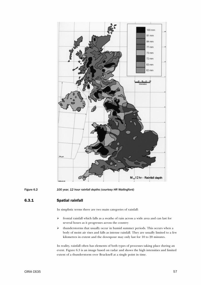
CIRIA C635 57

Figure 6.2 100 year, 12 hour rainfall depths (courtesy HR Wallingford)

6.3.1 Spatial rainfall

In simplistic terms there are two main categories of rainfall:

� frontal rainfall which falls as a swathe of rain across a wide area and can last for

several hours as it progresses across the country

� thunderstorms that usually occur in humid summer periods. This occurs when a

body of moist air rises and falls as intense rainfall. They are usually limited to a few

kilometres in extent and the downpour may only last for 10 to 20 minutes.

In reality, rainfall often has elements of both types of processes taking place during an

event. Figure 6.3 is an image based on radar and shows the high intensities and limited

extent of a thunderstorm over Bracknell at a single point in time.

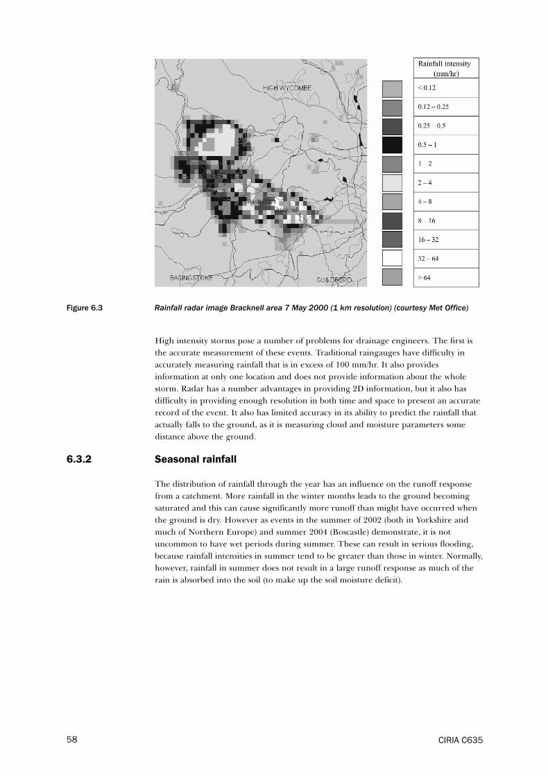
Figure 6.3 Rainfall radar image Bracknell area 7 May 2000 (1 km resolution) (courtesy Met Office)

High intensity storms pose a number of problems for drainage engineers. The first is

the accurate measurement of these events. Traditional raingauges have difficulty in

accurately measuring rainfall that is in excess of 100 mm/hr. It also provides

information at only one location and does not provide information about the whole

storm. Radar has a number advantages in providing 2D information, but it also has

difficulty in providing enough resolution in both time and space to present an accurate

record of the event. It also has limited accuracy in its ability to predict the rainfall that

actually falls to the ground, as it is measuring cloud and moisture parameters some

distance above the ground.

6.3.2 Seasonal rainfall

The distribution of rainfall through the year has an influence on the runoff response

from a catchment. More rainfall in the winter months leads to the ground becoming

saturated and this can cause significantly more runoff than might have occurred when

the ground is dry. However as events in the summer of 2002 (both in Yorkshire and

much of Northern Europe) and summer 2004 (Boscastle) demonstrate, it is not

uncommon to have wet periods during summer. These can result in serious flooding,

because rainfall intensities in summer tend to be greater than those in winter. Normally,

however, rainfall in summer does not result in a large runoff response as much of the

rain is absorbed into the soil (to make up the soil moisture deficit).

CIRIA C63558

6.4 Rural runoff

6.4.1 Characteristics of rainfall and rural runoff

Runoff characteristics of rural catchments are quite different from those of urban

catchments. With rural catchments, runoff depends primarily on the type of rainfall

and the nature of the catchment area, with a runoff hydrograph that is heavily

attenuated and a volume that is a function of the wetness of the soil. Table 6.1

summarises the rainfall runoff characteristics of rural catchments.

Table 6.1 Rainfall runoff characteristics for undeveloped areas

However the volume of runoff is only part of the issue. The rate of runoff is also

important. Rivers have base flows that are a function of rainfall as well as the

hydrogeology of the catchment. Rivers respond to rainfall in a matter of hours where

sufficient rain occurs. Runoff is rarely visible as overland flow except in the most

extreme conditions, and so the response to most rainfall is heavily attenuated. The

degree of attenuation is a function of the physical characteristics of the catchment.

The concept of frequency is important in the rainfall-runoff relationship. Frequency of

occurrence is related to the return period of the event. For a one in 50 year event

occurs on average once every 50 years, and will have an annual probability of

exceedance of 0.02. Probability of exceedance is the statistical probability of a hydrological

event (rainfall or flow) of a given magnitude being exceeded in any individual year.

Return period is the average time interval between occurrences of a hydrological event (rainfall

or flow) of a given or greater magnitude, usually expressed in years.

The probability of an event occurring or being exceeded during the system design life

can be determined using the following equation (Butler and Davies, 2004):

Pr = 1 - [1 – (1/T)]L (6.1)

where:

Pr = probability of event occurring or being exceeded within design life

T = return period

L = design life (years)

Using this equation the annual probability of exceedance has been calculated for a

range of return periods (Table 6.2). The table also includes the probability of an event

occurring during a 25 or 100 year design life.

CIRIA C635 59

Rainfall Catchment characteristics Catchment response

50 to 85 per cent of rainfall

events for all catchments.

Depending on soil type. No perceptible runoff.

Many events in winter.

Large summer events.

Response from less permeable

catchments.

Response in summer events normally

limited to steep catchments.

Small amount of runoff.

Extreme events, particularly

after an extended wet period.

Floods in winter.

Floods in summer normally limited to

steeper catchments.

Large amount of runoff.

Table 6.2 Probability of an extreme event happening

It should be noted that the return period of runoff is not the same as the rainfall event

for rural catchments. This is due to rainfall taking place on the days immediately prior

to the event making the catchment more liable to produce a flood response. The return

period of the flood response becomes proportionate to the rainfall as the catchment

becomes more developed (impermeable).

The return period of the events of interest to drainage engineers range from one to

200 years. Consideration of more extreme events is sometimes relevant, but usually

only when concerned with risk to life rather than flood damage. Consideration of

design exceedance and flood management is an open ended concept, but it should be

recognised that there comes a point where design will have limited influence in

managing the impact of a flood event. The flooding incident at Boscastle in 2004

illustrates that a rainfall event estimated at between 1000 and 5000 years (annual

probability of exceedance of up to 0.0002) cannot be managed directly. However it does

provide lessons in managing risk and protecting human life.

6.5 Models for estimating rural runoff

There are a number of tools available for estimating runoff from rural catchments,

however it should be recognised that rural areas are not homogenous. So the accuracy

of these tools will always be limited when not supported by reliable site measurement of

runoff rates.

There are three aspects to be determined when estimating runoff from rural areas:

� the volume of runoff

� the peak rate of flow

� the delay and shape of the runoff.

The next section looks at the methods available for estimating the peak flow rate and

this is followed by methods for estimating volumes of runoff. An example catchment is

then used to illustrate the differences between these methods.

The following methods are all regarded as “current” and no one method is considered

to be “right”, while the rest are “wrong”. However to avoid confusion a preferred

method is recommended as good practice. It is important to stress that using more than

one method can provide additional information on the decisions to be made. This can

be particularly useful in situations where the consequences of “failure” of a drainage

structure would be particularly serious. Table 6.3 summarises the various methods that

are currently used to determine peak flow rates and volumes of runoff. Appendix 7

provides a more complete summary of each of the methods and their formulae.

CIRIA C63560

Return period

(years)

Annual probability

of exceedance

Probability of exceedance during design life of…

25 years 50 years 100 years

2 50% ≈100% ≈100% ≈100%

5 20% ≈100% ≈100% ≈100%

10 10% 93% 99% ≈100%

30 3.33% 57% 82% 97%

50 2% 40% 64% 87%

100 1% 22% 39% 63%

200 0.50% 12% 22% 39%

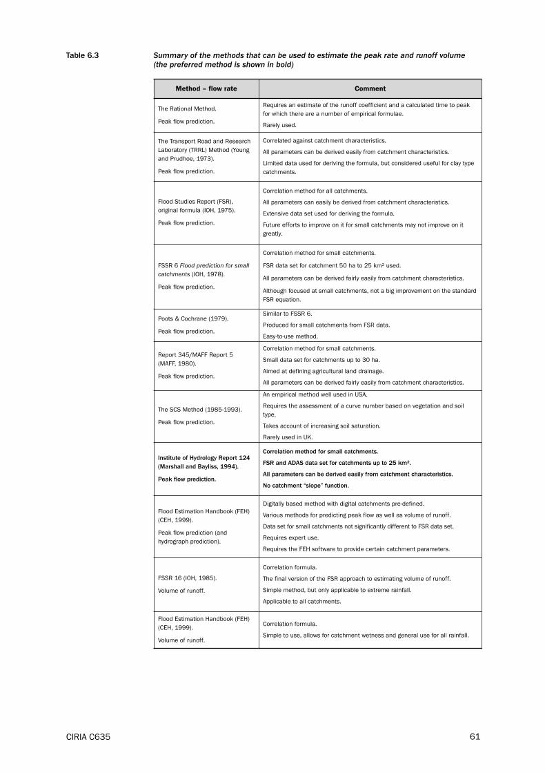
Table 6.3 Summary of the methods that can be used to estimate the peak rate and runoff volume(the preferred method is shown in bold)

CIRIA C635 61

Method – flow rate Comment

The Rational Method.

Peak flow prediction.

Requires an estimate of the runoff coefficient and a calculated time to peak

for which there are a number of empirical formulae.

Rarely used.

The Transport Road and Research

Laboratory (TRRL) Method (Young

and Prudhoe, 1973).


Correlated against catchment characteristics.

All parameters can be derived easily from catchment characteristics.

Limited data used for deriving the formula, but considered useful for clay type

catchments.

Flood Studies Report (FSR),

original formula (IOH, 1975).


Correlation method for all catchments.

All parameters can easily be derived from catchment characteristics.

Extensive data set used for deriving the formula.

Future efforts to improve on it for small catchments may not improve on it

greatly.

FSSR 6 Flood prediction for small

catchments (IOH, 1978).


Correlation method for small catchments.

FSR data set for catchment 50 ha to 25 km² used.

All parameters can be derived fairly easily from catchment characteristics.

Although focused at small catchments, not a big improvement on the standard

FSR equation.

Poots & Cochrane (1979).


Similar to FSSR 6.

Produced for small catchments from FSR data.

Easy-to-use method.

Report 345/MAFF Report 5

(MAFF, 1980).



Small data set for catchments up to 30 ha.

Aimed at defining agricultural land drainage.

All parameters can be derived fairly easily from catchment characteristics.

The SCS Method (1985-1993).


An empirical method well used in USA.

Requires the assessment of a curve number based on vegetation and soil

type.

Takes account of increasing soil saturation.

Rarely used in UK.

Institute of Hydrology Report 124

(Marshall and Bayliss, 1994).



FSR and ADAS data set for catchments up to 25 km².

All parameters can be derived easily from catchment characteristics.

No catchment “slope” function.

Flood Estimation Handbook (FEH)

(CEH, 1999).

Peak flow prediction (and

hydrograph prediction).

Digitally based method with digital catchments pre-defined.

Various methods for predicting peak flow as well as volume of runoff.

Data set for small catchments not significantly different to FSR data set.

Requires expert use.

Requires the FEH software to provide certain catchment parameters.

FSSR 16 (IOH, 1985).

Volume of runoff.

Correlation formula.

The final version of the FSR approach to estimating volume of runoff.

Simple method, but only applicable to extreme rainfall.

Applicable to all catchments.


(CEH, 1999).

Volume of runoff.

Correlation formula.

Simple to use, allows for catchment wetness and general use for all rainfall.

Where an estimate of peak flow is required to provide a reasonable basis for producing

design criteria for stormwater management of a site, it is recommended that IOH

Report 124 is used as the preferred method (good practice), with linear interpolation

for flows from areas smaller than 50 ha (Marshall and Bayliss, 2004).

Where an estimate of peak flow is required to provide for sizing of a culvert or other

structure where “failure” may have damage implications, appropriate consideration

should be given by supplementing the result from IOH Report 124 with some of the

other methods. An example of this is shown in Box 6.1. The selection of the other

methods depends to some extent on the catchment being considered.

Where a catchment has a significant urban area, the fraction of the catchment that is

developed should not be greater than 15 per cent to safely apply these formulae.

Where this exists it is advised that a more detailed assessment of the catchment is

carried out. This may include explicit modelling of both the rural and urban

components.

The prediction of rural runoff volume is becoming more important in setting criteria

for stormwater management. For extreme events the FSSR 16 method is the simplest

tool to use. Due to the nature of the formula an approximation of the percentage

runoff to the standard percentage runoff (SPR) value of the soil type can be made. For

small events and time series rainfall analysis the FEH model should be used. This

requires the use of a spreadsheet to assess the increasing CWI value and resulting

runoff using the hourly net rainfall through the event.

CIRIA C63562

Box 6.1 Example of calculating the peak runoff

The following example is a real catchment in the UK where the assessment of peak flow had to be

determined.

Catchment characteristics

The parameters that are needed for the various formulae have been measured or calculated. These are given

in Table 6.4.

Table 6.4 Catchment characteristics

It may be useful to carry out a simple

“sanity check” on the results, using a

simple Rational Method calculation,

before going into detail on the various

methods of analysis. The critical

duration of the catchment of these

characteristics is in the region of

around four to six hours. If one

assumes a constant rainfall of

10mm/hr taking place for four hours

(which is approximately a five to 10

year event for this location) and a

percentage runoff of 75 per cent for a

catchment of 1km², the flow rate

arriving at the culvert would be in the

region of 2m³/s. A high coefficient has been used to take account of the catchment shape and steep slope

and the class five soil type. So the various formulae would produce values of this order of magnitude for a 10

year event.

Table 6.5 provides the growth curve values for the region.

Table 6.5 Regional growth curve for the catchment

(This information is available from FSSR Reports 2 and 14 produced by the Institute of Hydrology and is based

on factoring QBAR, a measure of the mean annual event, to determine other events of greater magnitude).

Table 6.6 shows the results obtained from the formulae for a range of return periods.

CIRIA C635 63

Catchment area (km²) 0.88

Soil SPR 0.5 (type 5)

M5-2day (mm) 95

M5-1hr (mm) 22

URBAN 0

LAKE 0.01

RSMD 65

STMFRQ 3

ARF 0.99

SAAR (mm) 1489

Slope (S1085) 140

Return period 0.2 0.5 1 2 5

Growth factor 0.57 0.73 0.88 0.93 1.21

Return period 10 25 50 100 500 1000

Growth factor 1.42 1.71 1.94 2.18 2.86 3.19

CIRIA C63564

Box 6.1 (cont) Example of calculating the peak runoff

Table 6.6 Peak runoff (m³/s) assessment for the catchment (the preferred method is shown in bold)

* using the nomograph method

Figure 6.4 provides this information in a form that allows the variability of the results to be examined. It is

clear that for this type of catchment that the FEH methods would appear to be seriously under predicting the

peak flow for extreme events (even though they are the result of the most recent work). The implication from

this is that although there is a degree of agreement between various methods, the prediction of rural runoff

should be treated with caution.

In Figure 6.4 the prediction

of the peak flow by IOH

Report 124 is relatively low

and should not be used

exclusively for a situation

where an assessment for a

receiving pipe size is needed.

Conversely as an estimate for

assessing peak runoff criteria

for setting urban

development criteria it

provides a conservative

estimate. The receiving pipe

system, in this case, had a

maximum capacity of

between 1.25 and 1.5m³/s

Figure 6.4 Predicted peak flows for the catchment for various return periods

Method

Return

period

year

Return

period 2

year

Return

period 5

year

Return

period 10

year

Return

period 50

year

Prudhoe and Young (TRRL LR565) – 1.59 2.10 2.58 4.15

Flood Studies Report (IOH, 1975) six parameter method 1.53 1.62 2.11 2.48 3.38

FSSR 6: Flood prediction for small catchments (IOH) 1.45 1.53 1.99 2.34 3.19

ADAS 345 (extract from MAFF Report 5) * 1.41 – 1.85 2.38 –

Report 124 Flood estimation for small catchments (Marshall

and Bayliss, 1994)0.97 1.03 1.34 1.57 2.14

FEH – Analogy method (CEH, 1999) 0.32 0.34 0.47 0.56 0.82

FEH Statistical method (CEH, 1999) 0.54 0.57 0.78 0.94 1.37

4.5

4.0

3.5

3.0

2.5

2.0

1.5

1.0

0.5

0.0

1 10 100

Prudhoe & Young FSR FSSR 6 ADAS 345 IH 124 FEH 1 FEH 2

Return period

Flo

wm

/s3

7 Hydrological processes and the effects

of urbanisation

7.1 Hydrological processes

7.1.1 Introduction

Rainfall that falls on land can follow a number of different paths depending upon the

nature of the rainfall, the soil type, topography and land use (Figure 7.1). Usually only

a fraction of the total precipitation produces surface runoff, with the remaining either

intercepted before reaching the ground, infiltrated into the ground or lost back into

the atmosphere through evaporation and evapo-transpiration.

Figure 7.1 The hydrological process

7.1.2 Interception

Interception occurs when rain falls and is stored on vegetation, and subsequently

evaporates back to the atmosphere through transpiration. The amount of interception

depends on the nature of the vegetation, including plant type, form, the density of

leaves, branches and stems. Trees often have a high interception capacity compared

with grass which is substantially lower. Low rainfall events can be completely

intercepted but the proportion of interception for extreme rainfall events may be low.

7.1.3 Depression storage

Rainfall and through-fall below the vegetation cover may be trapped in puddles, ponds,

ditches or other depressions in the soil. The water retained in depression storage then

evaporates or infiltrates into the soil. The quantity of the depression storage is related

to the micro-topography and the properties of the soil surface.

CIRIA C635 65

7.1.4 Infiltration

Infiltration is the flow of water into the soil matrix. The infiltration rate depends upon

the nature of the soil and the soil moisture. Typically the infiltration rates for clays are

low while the infiltration rates for sands and gravels is high. Moist soils normally have

higher infiltration rates than dry soils. The water fills the voids between the soil

particles and the movement of the water is affected by both surface tension and gravity.

Water within the soil may be removed by the root systems of vegetation and

subsequently returned to the atmosphere through transpiration. The gravitational

force means that the flow of water in the unsaturated zone is predominantly vertical

until the water reaches the saturated zone, known as groundwater. Once within the

saturated zone the movement of the water tends to be horizontal.

7.1.5 Surface flow

If the rainfall intensity exceeds the infiltration capacity of the soil then water will form a

pond on the ground. The infiltration capacity of the soil is affected by the soil moisture,

the amount of surface runoff generated by a given rainfall event depends upon the

antecedent conditions. During extreme events if the rainfall is intense then a much

larger proportion becomes surface runoff than in less extreme events. This is because

the rate of rainfall is so great that runoff occurs even though infiltration is still taking

place.

The amount of infiltration that can take place may be severely limited if the ground is

frozen or baked hard as in the case of clay. The amount of surface runoff may be large.

7.1.6 Evaporation and evapo-transpiration

Water retained on the land surface, either through intercepted rainfall, depression

storage or in water bodies, is subject to evaporation. Water absorbed by the root

systems of plants returns to the atmosphere through evapo-transpiration. The amount

of evaporation and evapo-transpiration depends on the amount of solar radiation on a

particular day.

7.2 Runoff

Runoff is that proportion of the rainfall that appears in streams, rivers or drainage

systems as a discharge. It can come from surface and subsurface flow and from

groundwater. Subsurface runoff arises from water that has percolated through the soil

and drained directly to the stream. This subsurface runoff may contribute to stream

flow for some time after the rain has ceased. Where a river flows through an aquifer

there can be an exchange between the river and the aquifer. The direction of the flow

depends upon the relative levels of the water in the aquifer and the stream, and can

flow in either direction. Depending upon the size of the aquifer, it may be capable of

making a significant contribution to river flow for a long period of time.

The typical stream flow hydrograph for a single-storm event consists of:

� an initial low level of flow representing the base flow in the stream at the start of

the storm

� a rising limb resulting from surface runoff that starts a short time after the

beginning of the rainfall

� a peak when the discharge reaches a maximum

CIRIA C63566

� a decreasing limb as the rainfall diminishes

� a slow recession produced by groundwater flow after the rainfall ceases.

The recession is typically longer in duration than the rising limb. The shape of the

rising limb and the peak discharge depends upon:

� catchment characteristics such as topography, size, shape, stream network

development, geology

� initial conditions for example soil moisture and surface retention storage

� characteristics of the rainfall including the spatial and temporal distribution of

rainfall or snow melt.

In extreme events a larger proportion of the runoff may be in the form of surface

runoff than for less extreme events. This means that a much larger proportion of the

rainfall enters the river or drainage system rapidly rather than following slower routes

via infiltration. In extreme events, proportionally steeper hydrographs with larger peak

discharges may occur.

In discussing flood characteristics a number of parameters are commonly used. The

time of concentration is defined as the time required for a particle of water to travel

from the most distant point in the catchment to the outlet or the point under

consideration. The lag time can be defined as the time interval between the centroid of

effective rain and the peak of the discharge.

The time of concentration is affected by the size of the catchment. Small and steep

catchments have shorter times of concentration than large or flatter ones. The time of

concentration is important in deciding how a given catchment will respond to a

particular rainfall event. For rainstorms of the same probability, the intensity reduces

with duration. The intensity that is commonly experienced during a short summer

storm of five minutes duration is rarely sustained for periods of hours.

It has been observed that catchments respond differently to storms of different

durations. Small catchments respond most to shorter duration rainfall events while

larger catchments respond most to longer duration events. There is an interest in

estimating the critical storm duration for a given catchment. One of the assumptions of

the Rational Method is that a catchment gives the highest peak discharge for a storm

with a duration that approximates to the time of concentration of the catchment. If the

duration of the rainfall is less than the time of concentration then not all the catchment

has started to contribute to the runoff before the rainfall stops. If the duration of the

rainfall event is significantly longer than the time of concentration then the average

intensity of the rainfall will be less than that of a rainfall event whose duration matches

the time of concentration for any given return period. The implication is that for small,

steep catchments the highest peak flows are generated by short rainfall events of a few

hours while for a large, flat catchment the highest peak flows are generated by

extended rainfall events. This analysis assumes that rainfall is stationary relative to the

catchment and that the spatial distribution of rainfall is uniform. If the rainfall cell

moves relative to the catchment then this may modify the runoff flow rates. If a storm

cell tracks down the catchment then the impact of the runoff may be intensified while if

it tracks up a catchment then the impact may be diminished. The spatial distribution of

rainfall is rarely uniform over the whole catchment and this will also modify the runoff.

CIRIA C635 67

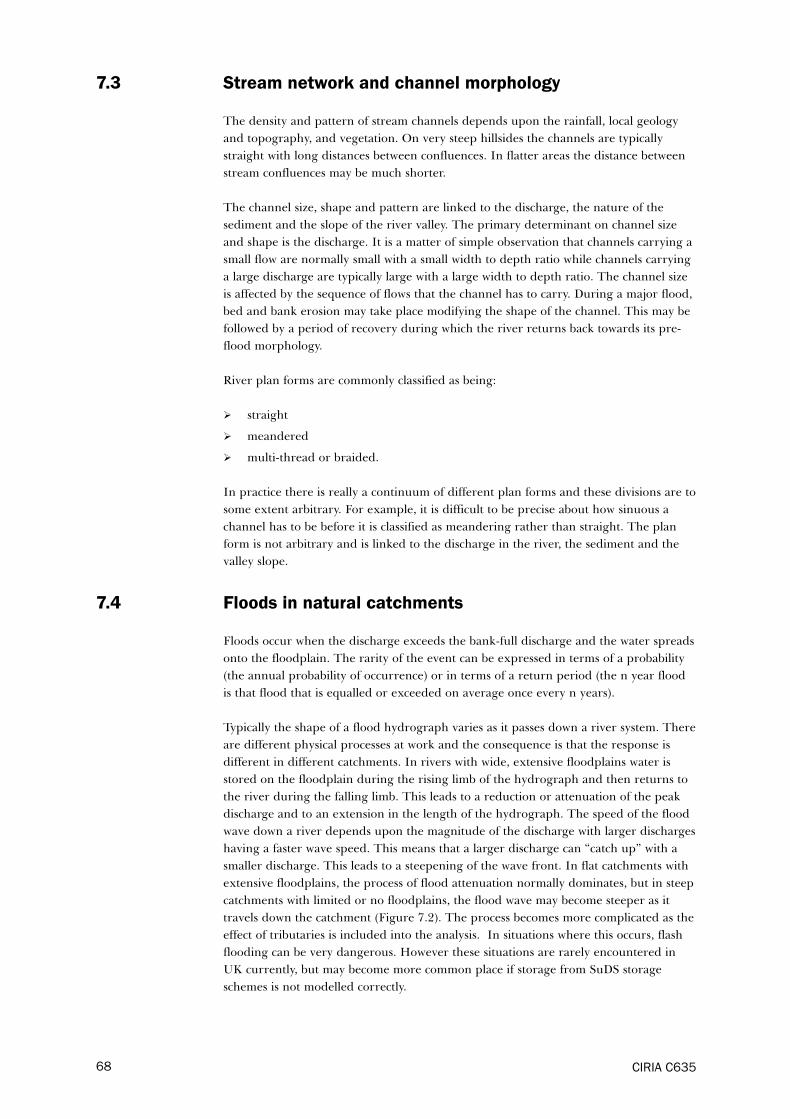
7.3 Stream network and channel morphology

The density and pattern of stream channels depends upon the rainfall, local geology

and topography, and vegetation. On very steep hillsides the channels are typically

straight with long distances between confluences. In flatter areas the distance between

stream confluences may be much shorter.

The channel size, shape and pattern are linked to the discharge, the nature of the

sediment and the slope of the river valley. The primary determinant on channel size

and shape is the discharge. It is a matter of simple observation that channels carrying a

small flow are normally small with a small width to depth ratio while channels carrying

a large discharge are typically large with a large width to depth ratio. The channel size

is affected by the sequence of flows that the channel has to carry. During a major flood,

bed and bank erosion may take place modifying the shape of the channel. This may be

followed by a period of recovery during which the river returns back towards its pre-

flood morphology.

River plan forms are commonly classified as being:

� straight

� meandered

� multi-thread or braided.

In practice there is really a continuum of different plan forms and these divisions are to

some extent arbitrary. For example, it is difficult to be precise about how sinuous a

channel has to be before it is classified as meandering rather than straight. The plan

form is not arbitrary and is linked to the discharge in the river, the sediment and the

valley slope.

7.4 Floods in natural catchments

Floods occur when the discharge exceeds the bank-full discharge and the water spreads

onto the floodplain. The rarity of the event can be expressed in terms of a probability

(the annual probability of occurrence) or in terms of a return period (the n year flood

is that flood that is equalled or exceeded on average once every n years).

Typically the shape of a flood hydrograph varies as it passes down a river system. There

are different physical processes at work and the consequence is that the response is

different in different catchments. In rivers with wide, extensive floodplains water is

stored on the floodplain during the rising limb of the hydrograph and then returns to

the river during the falling limb. This leads to a reduction or attenuation of the peak

discharge and to an extension in the length of the hydrograph. The speed of the flood

wave down a river depends upon the magnitude of the discharge with larger discharges

having a faster wave speed. This means that a larger discharge can “catch up” with a

smaller discharge. This leads to a steepening of the wave front. In flat catchments with

extensive floodplains, the process of flood attenuation normally dominates, but in steep

catchments with limited or no floodplains, the flood wave may become steeper as it

travels down the catchment (Figure 7.2). The process becomes more complicated as the

effect of tributaries is included into the analysis. In situations where this occurs, flash

flooding can be very dangerous. However these situations are rarely encountered in

UK currently, but may become more common place if storage from SuDS storage

schemes is not modelled correctly.

CIRIA C63568

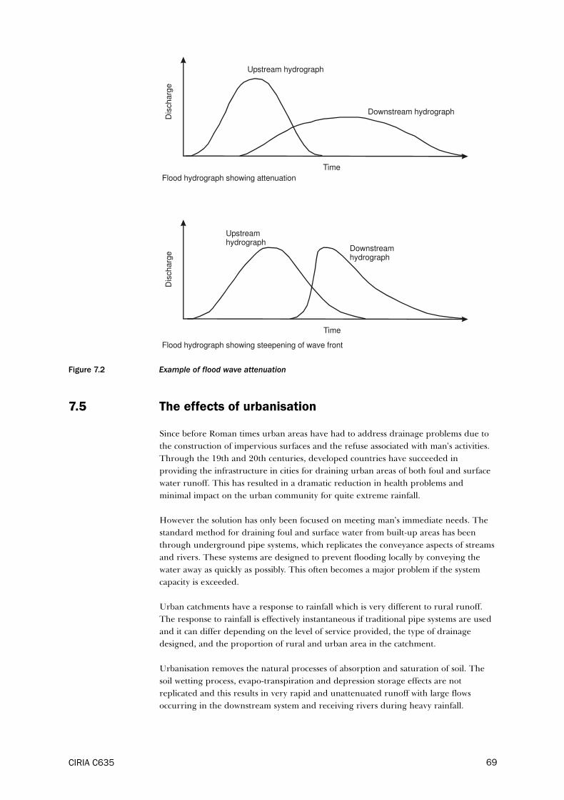
Figure 7.2 Example of flood wave attenuation

7.5 The effects of urbanisation

Since before Roman times urban areas have had to address drainage problems due to

the construction of impervious surfaces and the refuse associated with man’s activities.

Through the 19th and 20th centuries, developed countries have succeeded in

providing the infrastructure in cities for draining urban areas of both foul and surface

water runoff. This has resulted in a dramatic reduction in health problems and

minimal impact on the urban community for quite extreme rainfall.

However the solution has only been focused on meeting man’s immediate needs. The

standard method for draining foul and surface water from built-up areas has been

through underground pipe systems, which replicates the conveyance aspects of streams

and rivers. These systems are designed to prevent flooding locally by conveying the

water away as quickly as possibly. This often becomes a major problem if the system

capacity is exceeded.

Urban catchments have a response to rainfall which is very different to rural runoff.

The response to rainfall is effectively instantaneous if traditional pipe systems are used

and it can differ depending on the level of service provided, the type of drainage

designed, and the proportion of rural and urban area in the catchment.

Urbanisation removes the natural processes of absorption and saturation of soil. The

soil wetting process, evapo-transpiration and depression storage effects are not

replicated and this results in very rapid and unattenuated runoff with large flows

occurring in the downstream system and receiving rivers during heavy rainfall.

CIRIA C635 69

Upstream hydrograph

Downstream hydrograph

Flood hydrograph showing attenuation

Time

Flood hydrograph showing steepening of wave front

Upstreamhydrograph

Downstreamhydrograph

Dis

charg

e

Time

Dis

cha

rge

In addition, mankind, as a by-product of the highly intensive lifestyle and preference

for living in high density communities, generates a large number of pollutants. These

include sediments, oils, grits, metals, fertilisers, pesticides, animal wastes, salts,

pathogens and general litter and can cause extensive environmental damage. These

pollutants are collectively termed “urban diffuse pollution”. Rainwater mobilises many

of these pollutants which are then washed in to rivers and groundwater.

7.6 Urban runoff behaviour

Figure 7.3 shows the effect of three rainfall events (one, 30 and 100 year) and the runoff

response obtained from a traditional pipe based system using a simple model. This

shows an instant response for the one year event, with the thirty year event showing the

surcharge effect with a slightly attenuated peak flow, and the 100 year event being more

heavily attenuated as shown by the flat topped hydrograph. The flat topped hydrograph

indicates the constraining effects of the capacity of the piped drainage system and the

potential for surface flooding (note that the modelling approach does not fully allow for

overland flow effects and produces a slightly more “peaky” response).

However it can be seen that the timing of all of them is quick compared with the fourth

hydrograph which approximates to the runoff from a rural area of the same size for

the one year event. The relationship between rainfall and runoff is very direct and

proportional for urban runoff. Greenfield runoff for more extreme events with wet

antecedent conditions can result in more rapid runoff, and the figure provides a useful

illustration of the difference.

The response of the greenfield site is not only more delayed, but also much reduced in

volume of runoff. This shows that a mixed catchment of urban and rural runoff is likely

to result in a twin peaked hydrograph. The relative size of each of the peak flows is

dependent mainly on the proportion of urbanisation of the catchment, but also on the

size of the event and the soil type. This is illustrated by the two schematics in Figure

7.4. In both cases the catchment is assumed to be 10 per cent urbanised, and shows

hydrographs of both the rural runoff and paved runoff. The third hydrograph is the

combined flow. In the first figure the soil type is assumed to be relatively pervious

(sandy), while in the second the rural runoff is assumed to be from a clay catchment.

Figure 7.4 illustrates that once development is in the region of 10 per cent that the

response from the paved area may dominate the runoff in terms of flow rate even

though the volume of runoff from the pervious area is larger over a period of time.

These figures have used the simple assumption that a paved surface generates 100 per

cent runoff for the rainfall that falls on it. Similarly it has been assumed that the

percentage runoff from the soils are 30 per cent and 47 per cent respectively. For more

information on runoff from natural catchments, see Chapter 6.

The assumption that 100 per cent runoff is generated from paved surfaces is very

conservative and much work has been carried out to develop other runoff models

which provide a more accurate prediction of runoff. There are several urban runoff

models Chapter 8 provides an overview of these models, together with their advantages

and limitations.

CIRIA C63570

Figure 7.3 The response of a traditional pipe system to one, 30 and 100 year events compared with agreenfield response

Figure 7.4 The response from two catchments (soil types 2 and 4) with a development proportion of10 per cent, for the 100 year event

CIRIA C635 71

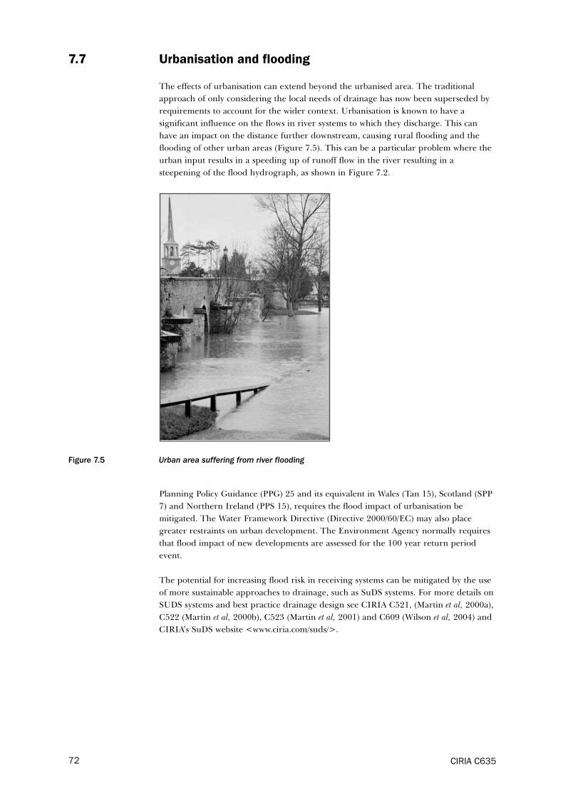
72 CIRIA C635

7.7 Urbanisation and flooding

The effects of urbanisation can extend beyond the urbanised area. The traditional

approach of only considering the local needs of drainage has now been superseded by

requirements to account for the wider context. Urbanisation is known to have a

significant influence on the flows in river systems to which they discharge. This can

have an impact on the distance further downstream, causing rural flooding and the

flooding of other urban areas (Figure 7.5). This can be a particular problem where the

urban input results in a speeding up of runoff flow in the river resulting in a

steepening of the flood hydrograph, as shown in Figure 7.2.

Figure 7.5 Urban area suffering from river flooding

Planning Policy Guidance (PPG) 25 and its equivalent in Wales (Tan 15), Scotland (SPP

7) and Northern Ireland (PPS 15), requires the flood impact of urbanisation be

mitigated. The Water Framework Directive (Directive 2000/60/EC) may also place

greater restraints on urban development. The Environment Agency normally requires

that flood impact of new developments are assessed for the 100 year return period

event.

The potential for increasing flood risk in receiving systems can be mitigated by the use

of more sustainable approaches to drainage, such as SuDS systems. For more details on

SUDS systems and best practice drainage design see CIRIA C521, (Martin et al, 2000a),

C522 (Martin et al, 2000b), C523 (Martin et al, 2001) and C609 (Wilson et al, 2004) and

CIRIA’s SuDS website <www.ciria.com/suds/>.

8 Runoff from urban catchments

8.1 Urban runoff models

Urban runoff models are used to estimate the rainfall runoff proportion that is drained

by the stormwater system. Historically this was calculated using the Rational Method

and it was assumed that in urban environments 100 per cent runoff took place from

paved surface and no runoff occurred from pervious areas. In the production of the

Wallingford Procedure in 1981, a statistical runoff model was produced, and was

referred to as the UK runoff model. This was produced by the Institute of Hydrology

and was calibrated against measured flow data. This equation was subsequently

modified in 1991. To distinguish it from the first equation this was referred to as the

new UK runoff model. For more information, reference should be made to CIRIA

X108 Drainage for development sites – a guide (Kellagher, 2004).

Many drainage engineers will have experience in using these methods in computer

simulation models of drainage networks. The simulation process usually involves the

verification of the data and modelling approach using short-term flow surveys (based

on the field measurement of sewer flow and rainfall), and subsequent use in simulating

the effects of “design” events. How these models work is often misunderstood. The

following sections have been developed in order to give the reader a better

understanding of the runoff estimation models that are embedded in modern software

tools, and enable them to select and apply them more reliably when simulating the

effects of extreme events.

The process of constructing a model and the consideration of exceedance is shown in

Figure 8.1.

8.1.1 The constant (old UK) runoff model

The first Wallingford Procedure runoff model is now usually referred to as “the

constant runoff model” (or old UK runoff model). This runoff model assumes losses are

constant throughout a rainfall event (runoff does not increase as the catchment gets

wetter) and is defined by the Equation 8.1:

PR = 0.829 PIMP + 25.0SOIL + 0.078 UCWI – 20.7 (8.1)

where:

PR = percentage runoff

PIMP = percentage impermeability (contributing)

SOIL = an index of the water holding capacity of the soil

UCWI = urban catchment wetness index

Values of SOIL range from 0.15 to 0.5 which are obtained from the winter rainfall

acceptance potential (WRAP) map which was produced as part of the Wallingford

Procedure. It is also available with the FSR manual. The values are a function of the runoff

characteristics of each soil type found in the catchment. There are only five categories of

SOIL with soil types being grouped together on the basis of their runoff characteristics.

CIRIA C635 73

CIRIA C63574

Fig

ure

8.1

Pro

ce

ss o

f co

nst

ructi

ng

a d

rain

ag

e m

od

el

Ra

infa

llC

atc

hm

en

t A

rea

Dra

ina

ge

sys

tem

Ide

nti

fy h

ydro

logic

al

regio

nC

ho

ose

so

il ty

pe

Pip

e s

yste

mS

uD

S

Ch

oo

se d

esi

gn

sto

rm r

etu

rn

pe

rio

ds

an

d a

ra

nge

of

du

rati

on

s

No

te:

Su

DS

un

its

wit

h o

utl

et

co

ntr

ols

(e

g

po

nd

s) h

ave

lo

ng

cri

tica

l d

ura

tio

ns

De

term

ine

are

as

con

trib

uti

ng t

o r

un

off

De

fin

e c

on

trib

uti

ng p

erm

ea

ble

/

imp

erm

ea

ble

ru

no

ff a

rea

Ge

ne

rate

de

sign

ra

infa

ll

Ap

ply

ap

pro

pri

ate

ru

no

ff m

od

el

for

ea

ch r

un

off

are

a t

ype

Ap

ply

clim

ate

ch

an

ge

fa

cto

r

Ge

ne

rate

/ob

tain

tim

e s

eri

es

rain

fall

(if

req

uir

ed

)

Bu

ild

ro

ad

ne

two

rk a

nd

an

y like

ly f

loo

d r

ou

tin

g

into

ne

two

rk

De

fin

e/a

gre

e p

erf

orm

an

ce c

rite

ria

fo

r si

te

dis

cha

rge

an

d f

loo

din

g

De

fin

e p

lan

la

you

t o

f th

e

pip

e s

yste

m

Ide

nti

fy t

he

lo

cati

on

an

d

typ

e o

f a

ll S

uD

S u

nit

s

De

term

ine

ch

ara

cte

rist

ics

of

the

pip

e s

yste

m:

�p

ipe

siz

es

�in

vert

le

vels

�p

ipe

ro

ugh

ne

ss

�le

ngth

s

De

term

ine

ch

ara

cte

risti

cs o

f

ea

ch

Su

DS

un

it.

Typ

ica

l

ch

ara

cte

risti

cs i

nclu

de

:

�in

filt

rati

on

ra

te

�p

oro

sity

�p

lan

are

a

�d

ep

th/l

eve

l, l

en

gth

�w

ate

r ta

ble

de

pth

Ad

d s

yste

m

sto

rage

Bu

ild a

nd

ru

n d

eta

iled

ne

two

rk m

od

el

Is o

verl

an

d f

low

an

issu

e?

Do

es

it n

ee

d t

o b

e

est

ima

ted

?

Are

sto

rage

volu

me

s su

ffic

ien

t?

(ch

eck

in

itia

l d

esi

gn

valu

es)

Re

po

rt

No

Re

vie

w r

esu

lts

Re

-ru

n m

od

el

Re

-ru

n m

od

el fo

r cr

itic

al

du

rati

on

ra

infa

ll (a

nd

/or

tim

e s

eri

es)

Ge

ne

rate

sh

ort

er

or

lon

ge

r

du

rati

on

de

sign

ra

infa

ll e

ven

ts

Re

ass

es

cha

ract

eri

stic

s o

f

pip

e s

yste

m a

nd

Su

DS

un

its

De

cisi

on

Ha

s th

ecr

itic

al

du

rati

on

be

en

re

ach

ed

fo

r b

oth

ove

rla

nd

flo

od

ing a

nd

syst

em

sto

rage

?

Are

th

e

pre

dic

ted

flo

ws,

volu

me

s o

r fl

oo

din

g h

igh

er

tha

n t

he

allo

wa

ble

lim

its?

Inp

ut

Pro

cess

De

sign

asp

ect

Incr

ea

se r

un

off

sto

rage

an

d

att

en

ua

tio

n t

hro

ugh

th

e u

se

of

ad

dit

ion

al

Su

DS

un

its

or

pip

ed

sto

rage

Yes

Yes

No

Ke

y:

CIRIA C635 75

Fig

ure

8.1

Pro

ce

ss o

f co

nst

ructi

ng

a d

rain

ag

e m

od

el

(co

nt’

d)

Ou

tpu

t

Values of UCWI, a composite of two antecedent wetness parameters, is given in

Equation 8.2:

UCWI = 125 + 8 API 5 – SMD (8.2)

where:

API5 = five day antecedent precipitation index (mm)

SMD = soil moisture deficit

It should be noted that the equation is entirely statistical and that it is heavily

influenced by the value of PIMP, as expected. If the catchment wetness term and soil

term are ignored, then the percentage runoff for a fully (100 per cent) paved

catchment would be approximately 62 per cent (0.829 × 100 – 20.7).

Although the model has a constant proportion of runoff, it recognises that the average

runoff volume during an event is a function of the catchment wetness. A value of

around 100 is used when carrying out network design (a function of season and annual

average rainfall depth), but specific values of UCWI are calculated for real events.

UCWI can range from 0 to over 300 mm.

There is an assumed distribution of the runoff from the paved and pervious surfaces

which assumes that the pervious runoff has a runoff factor which is 10 per cent of the

paved rainfall-runoff factor. If the percentage runoff from the paved area is calculated

to be 68 per cent, the value for the pervious surface would be 6.8 per cent. The model

is applied to urban areas without taking into account topography.

However it became clear that where the equation was applied to areas where the

contributing paved proportion was less than 30 per cent, unrealistically low values for

PR (percentage runoff) were being produced. Rules were created to try and avoid this

problem, but it was recognised that the constant runoff approach, irrespective of storm

depth and certain other limitations, needed to be improved. Figure 8.2 illustrates the

low values of PR which are produced by the equation. An override was later introduced

to ensure that where the PR value for the paved surface could not be less than 20 per

cent. However it is obvious that when this rule comes into effect that the equation is

being used beyond its limits.

Figure 8.2 PR as a function of SOIL and PIMP (old UK PR equation)

CIRIA C63576

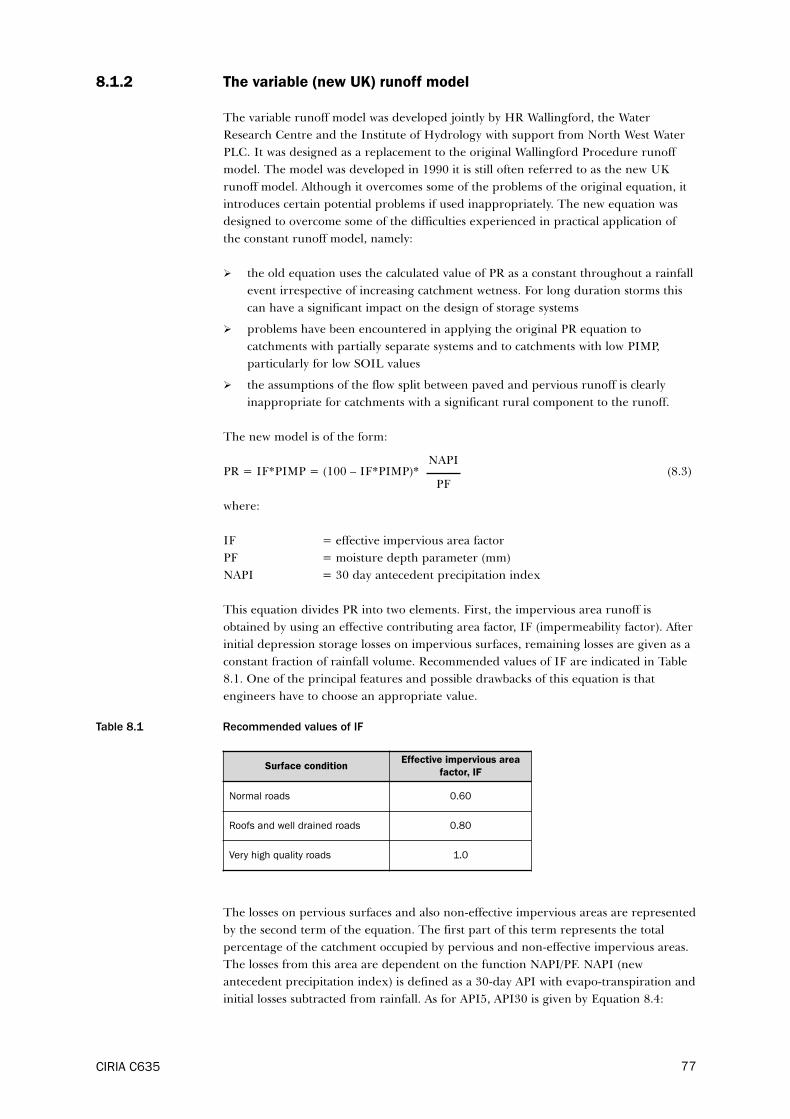
8.1.2 The variable (new UK) runoff model

The variable runoff model was developed jointly by HR Wallingford, the Water

Research Centre and the Institute of Hydrology with support from North West Water

PLC. It was designed as a replacement to the original Wallingford Procedure runoff

model. The model was developed in 1990 it is still often referred to as the new UK

runoff model. Although it overcomes some of the problems of the original equation, it

introduces certain potential problems if used inappropriately. The new equation was

designed to overcome some of the difficulties experienced in practical application of

the constant runoff model, namely:

� the old equation uses the calculated value of PR as a constant throughout a rainfall

event irrespective of increasing catchment wetness. For long duration storms this

can have a significant impact on the design of storage systems

� problems have been encountered in applying the original PR equation to

catchments with partially separate systems and to catchments with low PIMP,

particularly for low SOIL values

� the assumptions of the flow split between paved and pervious runoff is clearly

inappropriate for catchments with a significant rural component to the runoff.

The new model is of the form:

PR = IF*PIMP = (100 – IF*PIMP)* (8.3)

where:

IF = effective impervious area factor

PF = moisture depth parameter (mm)

NAPI = 30 day antecedent precipitation index

This equation divides PR into two elements. First, the impervious area runoff is

obtained by using an effective contributing area factor, IF (impermeability factor). After

initial depression storage losses on impervious surfaces, remaining losses are given as a

constant fraction of rainfall volume. Recommended values of IF are indicated in Table

8.1. One of the principal features and possible drawbacks of this equation is that

engineers have to choose an appropriate value.

Table 8.1 Recommended values of IF

The losses on pervious surfaces and also non-effective impervious areas are represented

by the second term of the equation. The first part of this term represents the total

percentage of the catchment occupied by pervious and non-effective impervious areas.

The losses from this area are dependent on the function NAPI/PF. NAPI (new

antecedent precipitation index) is defined as a 30-day API with evapo-transpiration and

initial losses subtracted from rainfall. As for API5, API30 is given by Equation 8.4:

CIRIA C635 77

NAPI

PF

Surface conditionEffective impervious area

factor, IF

Normal roads 0.60

Roofs and well drained roads 0.80

Very high quality roads 1.0

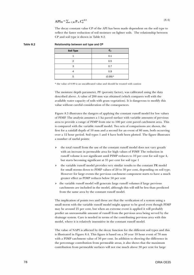
(8.4)

The decay constant value CP of the API has been made dependent on the soil type to

reflect the faster reduction of soil moisture on lighter soils. The relationship between

CP and soil type is shown in Table 8.2.

Table 8.2 Relationship between soil type and CP

* the value of 0.99 is an uncalibrated value and should be treated with caution

The moisture depth parameter, PF (porosity factor), was calibrated using the data

described above. A value of 200 mm was obtained (which compares well with the

available water capacity of soils with grass vegetation). It is dangerous to modify this

value without careful consideration of the consequences.

Figure 8.3 illustrates the dangers of applying the constant runoff model for low values

of PIMP. The analysis assumes a 1 ha paved surface with variable amounts of pervious

area to provide a range of PIMP from one to 100 per cent paved catchment area. This

is compared with the variable runoff model. Two sets of comparisons are shown, the

first for a rainfall depth of 10 mm and a second for an event of 80 mm, both occurring

over a 12 hour period. Soil types 1 and 4 have both been plotted. The figure illustrates

a number of useful points:

� the total runoff from the use of the constant runoff model does not vary greatly

with an increase in permeable area for high values of PIMP. The reduction in

runoff volume is not significant until PIMP reduces to 10 per cent for soil type 4,

but starts becoming significant at 35 per cent for soil type 1

� the variable runoff model provides very similar results to the constant PR model

for small storms down to PIMP values of 20 to 30 per cent, depending on soil type.

However for large events the pervious catchment component starts to have a much

greater effect as PIMP reduces below 50 per cent

� the variable runoff model will generate large runoff volumes if large pervious

catchments are included in the model, although this will still be less than predicted

from the same area by the constant runoff model.

The implication of points two and three are that the verification of a system using a

small storm with the variable runoff model might appear to be good even though PIMP

may be around 25 per cent, but when an extreme event is applied it will probably

predict an unreasonable amount of runoff from the pervious area being served by the

drainage system. Care is needed in terms of the contributing pervious area with this

model, where it is relatively insensitive in the constant runoff model.

The value of NAPI is affected by the decay function for the different soil types and this

is illustrated in Figure 8.4. This figure is based on a 50 year 18 hour event of 78 mm

with a PIMP catchment value of 50 per cent. In addition to showing the difference in

the percentage contribution from permeable areas, it also shows that the maximum

contribution from permeable surfaces will not rise much above 30 per cent for large

CIRIA C63578

Soil Type CP

1 0.1

2 0.5

3 0.7

4 0.9

5 (0.99)*

events on fairly impermeable soil types. It can be seen from the total runoff curves that

the effective paved area contribution is 60 per cent and that this is a constant

contribution.

As with the constant runoff model, it is worth briefly examining the likely maximum

value of percentage runoff from this model. For IF of 0.75, this means that for a

catchment which is 100 per cent paved, 25 per cent of the area is non-effective paved

surface and treated as part of the permeable catchment. If a storm depth of 80 mm is

assumed and no decay in the runoff function is allowed for, then the total runoff that

takes place is: 75% + 25% × (80/200) which is 85%

Figure 8.3 Volume of runoff from a 1 ha paved catchment with a variable amount of pervious area -(constant and variable runoff models)

Figure 8.4 Percentage runoff as a function of rainfall depth using the variable runoff model

CIRIA C635 79

8.1.3 The fixed percentage runoff model

The discussion on the Wallingford Procedure runoff models has highlighted the risks

in using these equations even though they are based on calibrated data. It is important

to make use of a simpler approach where reasonable approximations can be made

without losing too much accuracy.

The fixed percentage runoff model is simple to use and, in appropriate circumstances,

can be used without undue concern over its accuracy. The assumption used in Sewers

for adoption 5th edition that 100 per cent runoff takes place from all paved surfaces and

none from pervious areas is generally conservative for urban areas and realistic for

short duration and lower intensity events. Variations on this theme exist elsewhere. In

Belgium 80 per cent runoff from paved areas and zero from pervious surfaces is

commonly used for verifying models, which can involve the use of small storm events.

Where an allowance for pervious runoff is believed to be needed, values up to 30 per

cent are used depending on the circumstance.

A health check for using this simple approach can be made by comparing the fixed

percentage runoff used by Sewers for adoption 5th edition with the variable runoff model.

Figure 8.5 illustrates the difference in runoff proportion for various levels of PIMP, for

soil types 1 and 4, and for four storm events. The results show that, for fairly high

urban densities, the assumptions of 100 per cent and 0 per cent runoff, for paved and

pervious areas respectively, are cautious but provide a reasonable estimate for

predicting volumes of runoff. For large storms some provision for pervious runoff

becomes more important as PIMP reduces. However, this assumption is not advisable

for PIMP levels which are less than 50 per cent.

Figure 8.5a Comparison of percentage runoff between the variable runoff model and fixed percentagemodel used in Sewers for adoption 5th edition (2001) for a one year return period storm ofsix hour duration

CIRIA C63580

Figure 8.5b Comparison of percentage runoff between the variable runoff model and fixed percentagemodel used in Sewers for adoption 5th edition (2001) for a one year return period storm of24 hour duration

Figure 8.5c Comparison of percentage runoff between the variable runoff model and fixed percentagemodel used in Sewers for adoption 5th edition (2001) for a 100 year return period storm ofsix hour duration

Figure 8.5d Comparison of percentage runoff between the variable runoff model and fixed percentagemodel used in Sewers for adoption 5th edition (2001) for a 100 year return period storm of24 hour duration

CIRIA C635 81

8.2 Estimation of the difference between greenfield and

development runoff

Section 6.4 and Appendix 6 on rural runoff provide the tools to enable an assessment

to be made of the difference between a site before and after development. This is

important if design criteria are based upon the measurement of these differences. The

difference in runoff rates has been shown to be significantly so the rate of runoff from a

paved area needs to be physically controlled to achieve flow rates equivalent to

greenfield runoff. It is not necessary to determine the unrestrained runoff rate for the

paved area. However the same is not true of runoff volume.

Examination of the formula in FSSR 16 demonstrates that an approximation to SPR is

valid for extreme events for the respective soil type. Unfortunately this means that soil

types 4 or 5 which have SPR values around 50 per cent can be larger than the

predicted runoff from the catchment after development. Examination of Figure 8.3

shows that for a catchment with a PIMP of 50 per cent, it is possible to get a percentage

runoff predicted from a large event of around the same amount. This intuitively is

incorrect as the calibrated models of the Wallingford Procedure suggests that paved

areas have a runoff proportion in the region of at least 60 per cent and up to 85 per

cent. It would seem inappropriate that less runoff is predicted for the development

scenario than pre-development.

Careful consideration of the built environment provides some support for this result.

Developments involve the construction of not only buildings and roads, but also involve

the re-contouring of the area. Runoff from pervious areas may not be possible from

back gardens or low areas created by the development process. So where the pre-

development situation reasonably assumed that the whole catchment contributed to the

runoff, this may no longer be the case once development has taken place. Figure 8.6

shows a good recent housing development plan where much of the green area is to be

found in back gardens behind terraced houses.

It is important to be able to differentiate between areas that can and cannot contribute

runoff to the drainage system. Similarly, when using infiltration systems, the proportion

of the paved area that drains to a watercourse may only be a proportion of the total

hard surface area. These issues together with the rather complex and sometimes

awkward issues of using the appropriate runoff equation, means that a simple and easy

to use approach to quantify the difference between runoff volumes before and after

development is desirable.

CIRIA C63582

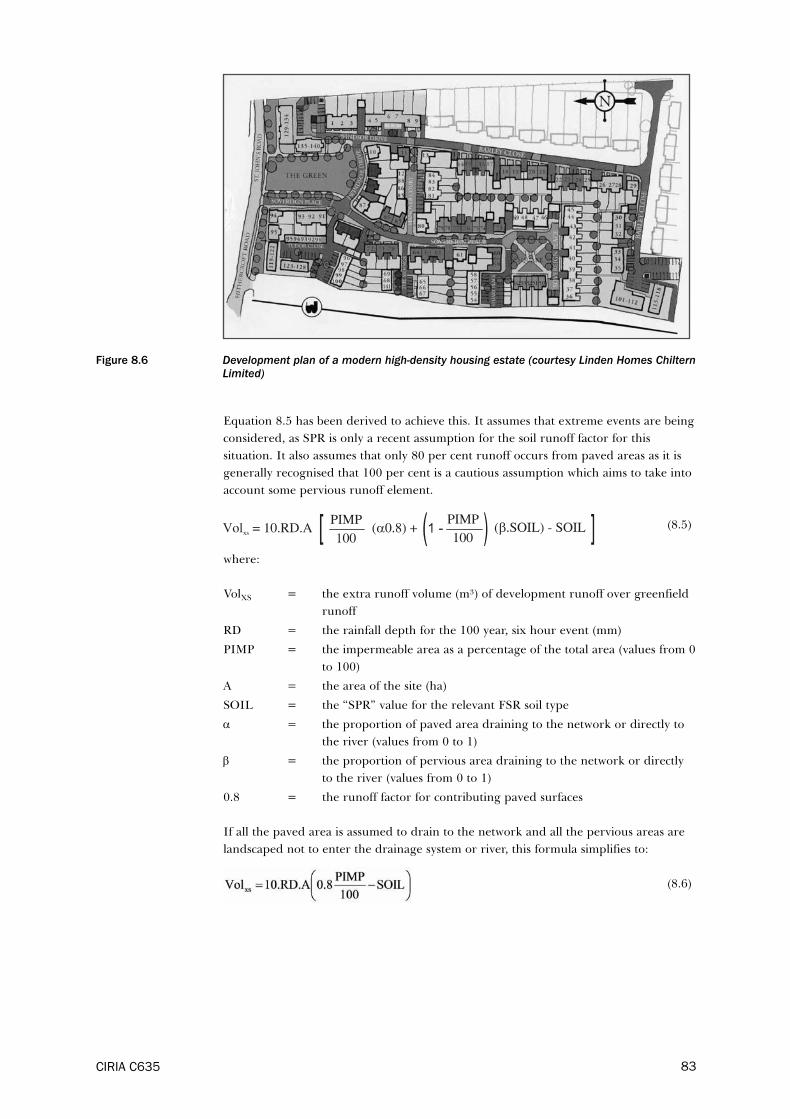
Figure 8.6 Development plan of a modern high-density housing estate (courtesy Linden Homes ChilternLimited)

Equation 8.5 has been derived to achieve this. It assumes that extreme events are being

considered, as SPR is only a recent assumption for the soil runoff factor for this

situation. It also assumes that only 80 per cent runoff occurs from paved areas as it is

generally recognised that 100 per cent is a cautious assumption which aims to take into

account some pervious runoff element.

(8.5)

where:

VolXS = the extra runoff volume (m³) of development runoff over greenfield

runoff

RD = the rainfall depth for the 100 year, six hour event (mm)

PIMP = the impermeable area as a percentage of the total area (values from 0

to 100)

A = the area of the site (ha)

SOIL = the “SPR” value for the relevant FSR soil type

α = the proportion of paved area draining to the network or directly to

the river (values from 0 to 1)

β = the proportion of pervious area draining to the network or directly

to the river (values from 0 to 1)

0.8 = the runoff factor for contributing paved surfaces

If all the paved area is assumed to drain to the network and all the pervious areas are

landscaped not to enter the drainage system or river, this formula simplifies to:

(8.6)

CIRIA C635 83

But where all pervious areas are assumed to continue to drain to the river or network

the formula becomes:

(8.7)

Figures 8.7 and 8.8 illustrate the difference in runoff volume for these two extremes

(fully disconnected/fully connected pervious surfaces) for the five different soil types for

any development density. To obtain a volume all that is required is to multiply the X-

axis value by the catchment area and the rainfall depth.

These graphs demonstrate the difference in soil type, the importance of using

infiltration to disconnect impermeable areas from the drainage network and the need

to be efficient in designing the general landscape to disconnect pervious areas.

This provides a rapid and robust easy-to-use method for assessing the additional

volume of runoff generated by any development.

Figure 8.7 Difference in runoff volume for developments where all pervious areas are assumed not todrain to the drainage network

Figure 8.8 Difference in runoff volume for developments where all pervious areas are assumed todrain to the drainage network

CIRIA C63584

9 Interaction between major and minor

systems

9.1 Principles of interaction

This chapter defines the mechanisms of interaction between the major and minor

drainage systems. It identifies when the major system comes into operation and gives

guidance as to how the user may determine the flows and volumes conveyed on the

surface by the major system, in specific circumstances. Interaction between the minor

and major drainage systems is complex. Above ground flow that causes the major

system to come into operation is known as the exceedance flow, and may be generated

from four sources:

� flooding from manholes and other connections to the minor system resulting from

a lack of capacity in the minor drainage system, or blockage, collapse or other

service defects

� excess surface runoff that cannot enter the minor system due to the limited

capacity of drainage inlets

� surface runoff from permeable areas that have no direct connection to the

sewerage network

� flooding caused by high levels in receiving waters preventing sewerage systems

from draining effectively.

During an extreme event, exceedance flows will travel on the surface in flood pathways.

These may consist of existing roads, paths and natural depressions in the ground.

Where they are not specifically designed as surface flood pathways (designed pathways)

they are known as default pathways. Such pathways can transfer flow over significant

distances so that flooding can occur at locations remote from the point of discharge

from the drainage system.

Although sewerage undertakers are required to keep records of sewer flooding

incidents, such records are often not sufficiently detailed to enable the cause of the

flooding to be reliably determined. When surface flooding is observed it is often very

difficult to ascertain the underlying cause by observation alone (Figure 9.1). In some

cases flooding can be the result of all four of the causes set out above which may

complicate the situation.

The processes governing the various interactions between the major and minor system

are complex and require a suitable level of analysis and supporting data if reliable

results are to be obtained. Interactions between inputs, processes and outputs are

illustrated in Figure 9.2 and described in the subsequent text.

CIRIA C635 85

Figure 9.1 Urban flooding illustrating the difficulty of identifying the precise cause of flooding

9.1.1 Flooding from manholes and other drainage connections

This condition describes the case where the flow in a piped drainage system becomes

such that it exceeds the capacity of that part of the system. This causes flow to back up

into manholes and gullies, and flooding can then occur when the level in the manhole

or gully rises above ground level. Flooding can also occur where a property, or part of

a property such as a cellar, lies below the level of the hydraulic gradient in the drainage

system. For this to occur there should be a pathway between the drainage system and

the property. This does not have to be an actual pipe connection, as there is plenty of

evidence of property flooding where no formal connection to the drainage system

exists. Cellared properties are particularly vulnerable to this form of flooding.

Modern computer simulation software can accurately replicate these conditions provided

that the connections between the minor and major systems are modelled. The volume of flooding

on the surface at a particular node (manhole or other point of connection) can be

predicted, and a depth of flooding can be deduced if the area of flooding is known.

How such surface flooding may be conveyed above ground by the major system (Figure

2.1), and what the consequential effects might be, has not been assessed historically.

This is because of the lack of guidance about how this should be done, and limitations

in the available terrain data (see Appendix 1). However, evidence of urban flooding

shows that overland flow is very important in determining the risk of flooding of

individual property.

CIRIA C63586

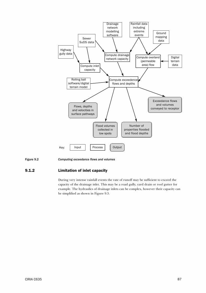
Figure 9.2 Computing exceedance flows and volumes

9.1.2 Limitation of inlet capacity

During very intense rainfall events the rate of runoff may be sufficient to exceed the

capacity of the drainage inlet. This may be a road gully, yard drain or roof gutter for

example. The hydraulics of drainage inlets can be complex, however their capacity can

be simplified as shown in Figure 9.3.

CIRIA C635 87

Drainage

network

modelling

software

Rainfall data

including

extreme

eventsGround

mapping

dataSewer

SuDS data

Highway

gully data

Digital

terrain

data

Compute drainage

network capacityCompute overland

(permeable

area) flow

Compute exceedence

flows and depths

Compute inlet

capacity

Rolling ball

software/digital

terrain model

Input ProcessKey:

Flows, depths

and velocities in

surface pathways

Exceedance flows

and volumes

conveyed to receptor

Flood volumes

collected in

low spots

Number of

properties flooded

and flood depths

Output

Figure 9.3 Conceptual model of exceedance due to inlet capacity

Point C in the figure shows the capacity of the inlet, defined by the flow Qc. Up to this

point all the surface runoff is passed into the minor system, as represented by the 1:1

relationship of the line OC. Beyond this point excess flow (exceedance flow) is diverted

to the major system. As depths of flow on the surface increase, it is possible that further

flow may be forced into the inlet, so that there is a further increase in minor system

flow, as indicated by the line CD. The slope of CD will be largely governed by the

hydraulic characteristics of the inlet.

The exceedance flow in the major (above ground) system will be the difference between

the surface runoff and the inlet flow, as illustrated in the figure. Some inlets such as

roof gutters may restrict the inflow such that the line CD is almost horizontal, and the

excess flow beyond C is diverted to the major system. Others, such as highway gullies,

may allow almost all the additional flow to enter as depths and flows increase, being

limited only by the capacity of the connection to the piped system. In practice the

transition may not be as abrupt as it is shown in the figure, the part CD may not be

linear, and the characteristic may have more than two stages.

The simplified approach in Figure 9.3 has the advantage that it can easily be built up

for standard inlet components. Also, by aggregating the effect of sub-components, the

overall characteristic of a sub area can be built up. This will be useful in modelling large

catchment areas where the model detail does not extend to the head of the drainage

system. This is explained further in the case studies in Part C.

When reviewing records of flood events great care should be taken in interpreting

evidence of flooding. Photographic and video evidence may at first sight appear to

show inflow being restricted by the capacity of the inlet whereas the flow may not be

able to enter the piped system because it is already surcharged to ground level.

CIRIA C63588

Minor system

flow Major system

flow

Surface

runoff

C

E

D

Qc

O

1

1

9.1.3 Surface runoff from pervious area

Runoff from pervious areas adjacent to drained paved areas is known to contribute to

drainage flows (Figure 4.3). Some modern software tools explicitly allow for this.

The impact of overland flow from pervious surface runoff is increasingly seen as a

major factor in urban flooding. In the subsequent analysis of flooding in Glasgow East,

runoff from adjacent pervious areas was shown to contribute up to 34 per cent of the

total flood volume (Figure 5.3).

Where significant pervious areas are known to drain onto developed areas, their impact

during extreme events should always be assessed. When modelling the effects of

extreme events, these contributing areas should be explicitly included in the simulation

model with an appropriate runoff model (see Chapter 6).

9.2 Calculating exceedance flow

The interaction between the minor and major drainage systems is complex and

accurately assessing exceedance flow can also be complex and sometimes expensive.

The degree of resources in calculating exceedance flow should match the needs of a

particular project. In some cases a more approximate method can be justified whereas

in others (where the risk and/or impact is higher) a detailed analysis will be necessary.

This guide recommends a three level approach to calculating exceedance flow, as

illustrated in Box 9.1.

The user is encouraged to evaluate which level of study is appropriate in individual

circumstances based on the perceived level of flood risk. Further guidance on this is

given in Section 10.3. The levels of analysis may be applied progressively, and to

different parts of a drainage area as required. The overall process is illustrated in the

flowchart in Figure 9.4.

CIRIA C635 89

CIRIA C63590

Box 9.1 Levels of detail for calculating exceedance flow

Level 1 study

Design of new drainage in small developments (say up to 50-100 dwellings).

Simple dendritic drainage layout without complex ancillaries. This level is not suitable for analysing existing

systems.

Minor drainage system designed in conventional manner using Rational Method or suitable software tool.

Exceedance flow calculated on basis of minor drainage system at capacity ie all surface runoff from the extreme

event conveyed by the major system. Surface conveyance replicated by simplified dendritic layout of open

channels. Peak flows and volumes calculated using Rational Method or suitable software package. Contributing

pervious areas included as equivalent paved areas when using the Rational Method.

Level 2 study

Analysis/design of medium to large (>200 properties say) drainage systems with some degree of complexity.

Minor drainage system analysed/designed using sewer network modelling software capable of replicating

surcharging and surface flooding. For existing areas the sewer network model should be verified by comparison

with short term flow survey data or historic flooding data.

Surface conveyance represented by pathways identified by site inspection, or in conjunction with a “rolling ball”

model using digital terrain data. Low spots where floodwater may pond identified by site inspection or in

conjunction with a digital terrain model. Contributing pervious areas modelled explicitly. No allowance for inlet

capacity included.

Properties may be grouped into areas for the assessment of risk.

Level 3 study

Analysis/design of large and complex drainage systems.

Minor drainage system analysed/designed using sewer network modelling software capable of replicating

surcharging and surface flooding, including backwater effects. For existing systems the sewer network model

should be verified by comparison with short term flow survey data and historic flooding data.

Surface conveyance replicated by explicit modelling of known surface flood pathways with full interaction

between major and minor networks. Subsequent flooding analysed using “rolling ball” model. Contributing

pervious areas explicitly modelled. Allowance made for inlet capacity on an area or individual basis.

Property flood risk assessed on an individual property basis, including explicit allowance for floor levels and

cellars.

Fig

ure

9.4

Flo

wch

art

fo

r co

mp

uti

ng

exc

ee

da

nce

flo

ws

an

d v

olu

me

s

CIRIA C635 91

Se

lect

ext

rem

e e

ven

ts

for

an

aly

sis/

de

sign

Co

llect

da

ta o

n d

rain

age

an

d

sew

er

pip

ed

/Su

DS

sys

tem

Ide

nti

fy s

urf

ace

flo

od

pa

thw

ays

Bu

ild s

ew

er

ne

two

rk m

od

el

Co

llect

da

ta o

n s

urf

ace

flo

od

pa

thw

ays

Bu

ild d

en

dri

tic

ne

two

rk o

f

surf

ace

flo

od

pa

thw

ays

Bu

ild d

igit

al

terr

ain

mo

de

l

wit

h s

ite

in

spe

ctio

n

Ve

rify

se

we

r n

etw

ork

mo

de

l

Ru

n m

od

el

wit

h s

ele

cte

d

ext

rem

e e

ven

ts

Ide

nti

fy s

urf

ace

flo

od

pa

thw

ays

by

insp

ect

ion

Is a

dig

ita

l

terr

ain

mo

de

l

ava

ilab

le?

Is a

le

vel

1

stu

dy

ap

pro

pri

ate

?

Are

re

sult

s

suff

icie

ntl

y d

eta

iled

fo

r

pu

rpo

se o

f st

ud

y?

Yes

No

Yes

No

LEVEL 2 STUDY

Yes

No

LEVEL 1 STUDY

Re

vie

w h

ydra

ulic

gra

die

nt

an

d n

od

al

flo

od

vo

lum

es

Co

mp

ute

exc

ee

de

nce

flo

ws

in s

urf

ace

flo

od

pa

thw

ays

Re

po

rt

Ou

tpu

t

Fig

ure

9.4

Flo

wch

art

fo

r co

mp

uti

ng

exc

ee

da

nce

flo

ws

an

d v

olu

me

s (c

on

t’d

)

CIRIA C63592

Re

-ru

n m

od

el

wit

h s

ele

cte

d

ext

rem

e e

ven

ts

Div

ide

co

ntr

ibu

tin

g a

rea

s

an

d a

pp

ly l

imit

ing i

nle

t fl

ow

s

Ad

d s

urf

ace

flo

w p

ath

wa

ys

to m

od

el

LEVEL 2 STUDY

LEVEL 3 STUDY

Co

llect

fu

rth

er

terr

ain

da

ta

an

d a

dd

to

mo

de

l

Use

dig

ita

l te

rra

in m

od

el

an

d r

olli

ng b

all

too

l

Are

re

sult

s

suff

icie

ntl

y d

eta

iled

for

the

pu

rpo

se o

f th

is

stu

dy?

Re

-ru

n m

od

el

wit

h s

ele

cte

d

ext

rem

e e

ven

ts

Bu

ild s

urf

ace

flo

od

pa

thw

ays

in

to

ne

two

rk m

od

el

Ad

d p

rop

ert

y le

vel

to d

ata

an

d

ass

ign

pro

pe

rty

to n

od

es

De

cisi

on

Inp

ut

Pro

cess

Ke

y:

Re

vie

w r

esu

lts

Re

po

rt

9.3 Calculating flows in surface flood pathways

9.3.1 Surface runoff

Surface runoff may be calculated using the Rational Method (see Chapter 6), however

this method has significant limitations, especially in generating correct flow volumes.

Given the availability and ease of use of modern simulation software tools the Rational

Method is only recommended for use with very small areas and where significant major

system flow is not anticipated.

The above ground flood pathways may be defined as rectangular or vee section open

channels, with nodes at key junctions. When using the Rational Method these should

form a dendritic network ie avoiding loops. However loops are permitted with most

simulation software.

Contributing areas should be assessed in the usual way by drawing boundaries around

the curtilage of property. Contributing areas of different types should be distinguished

(eg roofs from ground level paved, and paved from permeable). Each area type should

be assigned a suitable percentage runoff value. Further details are given in Chapter 8.

If using the Rational Method each contributing area A can then be converted to an

equivalent impermeable area Ae, using the percentage runoff PR:

(9.1)

The peak rate of surface runoff may be obtained using the Rational Method. This

calculates flow using the following equation.

Q =2.78.Ai.i litres/sec (9.2)

where:

Ai = equivalent impermeable area in hectares

i = average rainfall intensity in mm/hr, based on a critical duration equal

to the time of concentration

The rainfall intensity i should be chosen for an appropriate return period of extreme

event, and for the critical duration (equal to the time of concentration). Further

guidance on this may be found in the Wallingford Procedure (Standing Technical

Committee on Sewers and Water Mains, 1981).

Simulation software tools normally allow for variations of rainfall intensity during storm

events and will assign specified PR values to contributing areas directly.

9.3.2 Adding runoff from permeable areas

Current drainage design practice is only to allow for runoff from permeable areas

where these are immediately adjacent to paved areas or where they are drained directly

to the sewerage system (eg through land drains). However, recent studies such as those

in Glasgow have shown that in extreme events these areas can significantly contribute

to urban flooding and so should be included in any computations of surface runoff for

extreme events, as described in Chapter 8.

CIRIA C635 93

When using the Rational Method, a permeable area may be represented by an

equivalent impermeable area using the PR value for conversion. However, it is

important to note that by representing permeable areas as equivalent impermeable

areas, the time of concentration will not be properly replicated. When using simulation

software, permeable areas should be properly specified and not represented as

equivalent impermeable areas. Further guidance on this is given in Chapter 8.

9.3.3 Surface conveyance

In level 1 studies the below ground sewer system is assumed to be full to capacity so

that all surface runoff is conveyed above ground. This is a significant simplification of

the real scenario and normally will lead to an over estimate of above ground flows. This

approach is only suitable for use in small developments where a conservative allowance

for surface conveyance is acceptable (eg new sewerage for small housing and industrial

developments). It should not be used for assessing exceedance conditions for existing

systems or medium to large sized new systems.

Major system flows may be determined either by the Rational Method or preferably by

computer simulation, by representing surface flood pathways as drainage channels.

Most software simulation tools will allow the user to specify the shape of the channel

cross-section as one of a number of standard types. Rectangular, vee and trapezoidal

are usually sufficient to replicate most surface pathways. Figure 9.5 shows how a typical

road cross-section may be represented by two vee section channels.

Figure 9.5 Road flood pathway represented by vee section channel

In specifying the equivalent vee section in Figure 9.5 the cross-sectional area of flow

below top of kerb level should remain the same. The slope of the road surfaces will also

be the same. The only change to the equivalent section will be the reduction to the

wetted perimeter on the vertical sides of the section. As this is small in terms of the

overall cross-section, its effect will be minimal.

(9.3)

Conveyance may be represented by the Manning Equation 9.3.

where:

Q = discharge, m³/s

n = Manning roughness value

R = hydraulic radius = A/P

s = slope (decimal)

AC = cross-sectional area of flow, m²

P = wetted perimeter, m

CIRIA C63594

Road cross-sectionEquivalent composite

vee section

Further information on the application of this equation is given in Chapter 11,

including recommended values for the Manning roughness coefficient n.

The Manning Equation may be solved by trial and error to determine the depth of

conveyance flow in an above ground pathway for a given discharge. It can also be used

for determining the velocity of flow and time of travel. In theory it can be used with the

Rational Method to compute flows and depths in above ground flow pathways.

However the method is tedious, and the engineer is advised to use an appropriate

software simulation tool instead (see Appendix 1). Some software simulations tools give

the user a choice of equations for replicating conveyance, usually between the Manning

Equation and the Colebrook-White Equation. This is discussed further in Chapter 11.

The engineer should carefully check values of computed depth in such channels to

ensure that the flow will remain within the assumed pathway. Where depths of flow

exceed the height of a drainage channel (eg kerb height) then the channel section

should be revised (eg extending the road section to back of footpath). Further

information on this can be found in Chapter 11 and Appendix 2.

In level 1 studies the above ground flood pathways may be represented by a dendritic

network. In the case of road junctions, this may require a decision as to which direction

forms the major flood path. This is not always obvious from a plan view and a site visit

is advisable where possible to ascertain direction of surface flows. Other flood pathways

may be included such as paths and grass lined channels designed especially to convey

above ground flood flow.

In level 2 studies it is assumed that there is no limit on drainage inlet capacity so that

all surface runoff is drained to the below ground system it is full. At this point any

additional runoff will induce surface flooding from manholes. In simpler models this

surface flooding may be distributed over known flooded areas adjacent to the manhole,

and the depth of flooding determined. This may in turn be used to estimate damage

cost to property etc and further information on this is contained in Chapter 10.

However, experience shows that flood water discharged from manholes often does not

remain in the vicinity of that manhole, and can travel some considerable distance,

affecting people and property remote from the point of discharge. The engineer

should account for such potential surface transmission of flood flows. In its simplest

form this can be done by site inspection, identifying potential flood pathways and low

spots where flood water might accumulate. This is a particularly useful method when

combined with records of known flooding. However unrecorded locations of flooding

can be missed and the method is time consuming when applied to larger areas.

Where topographical data is available this can be used to build a digital ground terrain

model, and the flood volume can then be transmitted along the line of maximum

ground slope, and accumulated in low spots. This technique is often referred to as a

“rolling ball” model and this can give a more accurate assessment of the location and

volume of flooding. Light detection and ranging (LiDAR) data for many of the major

cities is available based on 1 m grid sets with ±150 mm vertical accuracy. If this data is

not available, it can be obtained by commissioning a survey (Allitt, 2004).

The accuracy of rolling ball models depends on the accuracy and resolution of available

digital terrain data. These tend to give better results in undeveloped areas rather than

urban areas, because surface flood pathways in urban areas are often defined by

artificial features, often no more than some 50 mm in height. A good example is the

role of roads with kerb heights of no more than 100 mm. Currently most terrain level

data is not available to such resolution. This means that rolling ball models need to be

CIRIA C635 95

interpreted with care, and the engineer may need to supplement them by modelling

known major flood pathways explicitly.

Local watercourses in extreme events can significantly affect the performance of urban

drainage systems. High water levels can restrict the discharge from outfalls from surface

water sewers and combined sewer overflows. Where local water courses are thought to

interact with the sewerage system in this way an allowance should be made in the

model either by applying an appropriate level hydrograph to the outfalls or by

explicitly modelling the watercourses as part of the drainage network. Particular

attention should be paid to representing culverted sections and watercourse screens,

both of which may become blocked during extreme events. Where outfalls are known

to be affected by tide levels, this should modelled.

For level 3 studies, full interaction between major and minor systems may be simulated,

by modelling surface flood pathways linking nodes, as shown in Figure 9.6. How

surface flood pathways are represented will depend on the specific software used.

Further information on this is given in Appendix 1. Surface flooding may still occur in

such models when the flood pathways are overtopped, and the subsequent passage of

such flow to low spots may be simulated with a rolling ball model.

Figure 9.6 Conceptual representation of fully interactive major/minor system modelling (after Allitt, 1999)

In level 3 studies, individual property may be assigned to nodes so that flood risk can

be determined on an individual property basis. In assessing flood risk, due account

should be taken of the level of the hydraulic gradient with respect to property floor

levels, especially where properties have cellars. It should be remembered that a

significant proportion of property flooding occurs without flood flow being discharged

from manholes in the locality (ie before the hydraulic gradient reaches ground level).

Also, the inlet capacity of drainage should be simulated where it is likely to affect system

performance.

Highway gullies, yard gullies and roof gutters can have limited capacity and that

including these effects may be important in representing exceedance conditions in

large complex drainage systems. Further details of this are given in Section 9.4.

The effects of local watercourses and tide locked outfalls should be represented in the

same way as in level 2 studies.

CIRIA C63596

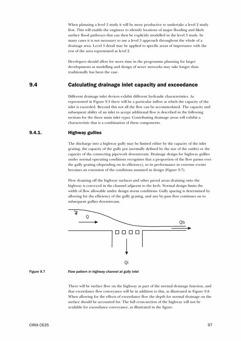
When planning a level 3 study it will be more productive to undertake a level 2 study

first. This will enable the engineer to identify locations of major flooding and likely

surface flood pathways that can then be explicitly modelled in the level 3 study. In

many cases it is not necessary to use a level 3 approach throughout the whole of a

drainage area. Level 3 detail may be applied to specific areas of importance with the

rest of the area represented at level 2.

Developers should allow for more time in the programme planning for larger

developments as modelling and design of sewer networks may take longer than

traditionally has been the case.

9.4 Calculating drainage inlet capacity and exceedance

Different drainage inlet devices exhibit different hydraulic characteristics. As

represented in Figure 9.3 there will be a particular inflow at which the capacity of the

inlet is exceeded. Beyond this not all the flow can be accommodated. The capacity and

subsequent ability of an inlet to accept additional flow is described in the following

sections for the three main inlet types. Contributing drainage areas will exhibit a

characteristic that is a combination of these components.

9.4.1. Highway gullies

The discharge into a highway gully may be limited either by the capacity of the inlet

grating, the capacity of the gully pot (normally defined by the size of the outlet) or the

capacity of the connecting pipework downstream. Drainage design for highway gullies

under normal operating conditions recognises that a proportion of the flow passes over

the gully grating (depending on its efficiency), so its performance in extreme events

becomes an extension of the conditions assumed in design (Figure 9.7).

Flow draining off the highway surfaces and other paved areas draining onto the

highway is conveyed in the channel adjacent to the kerb. Normal design limits the

width of flow allowable under design storm conditions. Gully spacing is determined by

allowing for the efficiency of the gully grating, and any by-pass flow continues on to

subsequent gullies downstream.

Figure 9.7 Flow pattern in highway channel at gully inlet

There will be surface flow on the highway as part of the normal drainage function, and

that exceedance flow conveyance will be in addition to this, as illustrated in Figure 9.8.

When allowing for the effects of exceedance flow the depth for normal drainage on the

surface should be accounted for. The full cross-section of the highway will not be

available for exceedance conveyance, as illustrated in the figure.

CIRIA C635 97

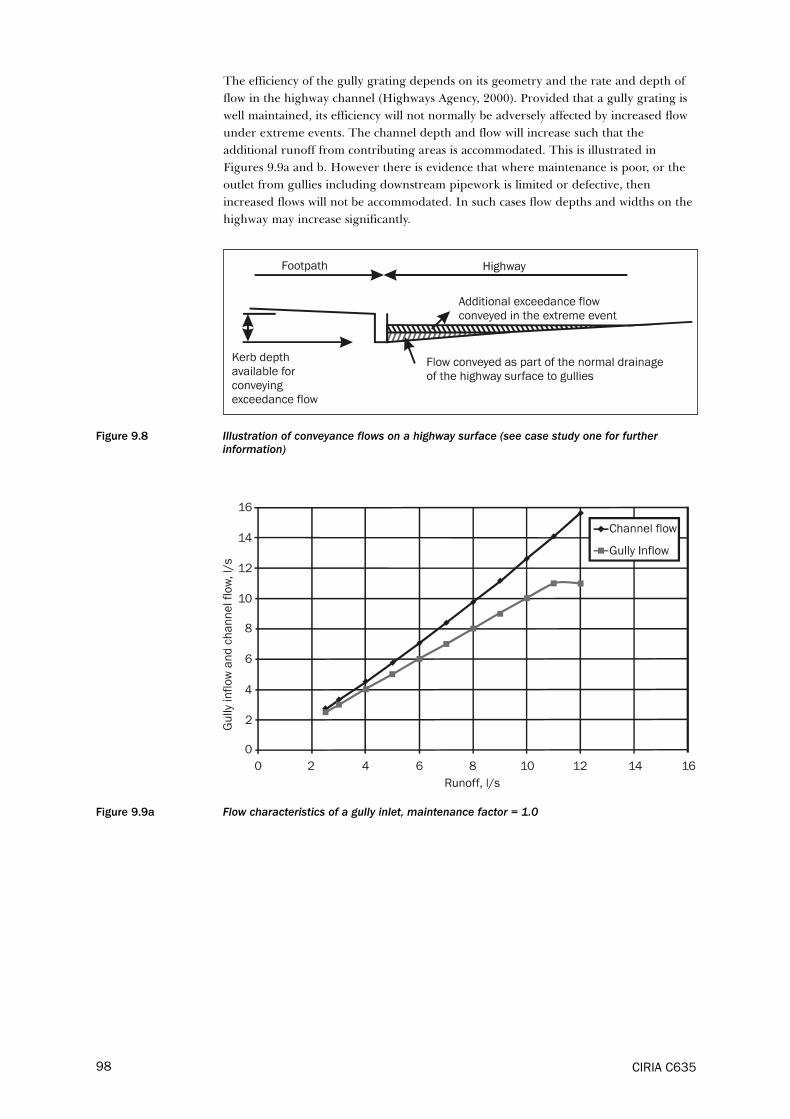
The efficiency of the gully grating depends on its geometry and the rate and depth of

flow in the highway channel (Highways Agency, 2000). Provided that a gully grating is

well maintained, its efficiency will not normally be adversely affected by increased flow

under extreme events. The channel depth and flow will increase such that the

additional runoff from contributing areas is accommodated. This is illustrated in

Figures 9.9a and b. However there is evidence that where maintenance is poor, or the

outlet from gullies including downstream pipework is limited or defective, then

increased flows will not be accommodated. In such cases flow depths and widths on the

highway may increase significantly.

Figure 9.8 Illustration of conveyance flows on a highway surface (see case study one for furtherinformation)

Figure 9.9a Flow characteristics of a gully inlet, maintenance factor = 1.0

CIRIA C63598

Figure 9.9b Flow characteristics of a gully inlet, maintenance factor = 0.7

Exceedance due to gully capacity is likely to occur in the following circumstances:

� the maintenance of all the inlet gratings in the area is so poor as to obscure a

significant part of the grating

� there are insufficient gullies for effective drainage of the area (ie less than the

normally recommended spacing)

� the runoff discharged to each individual gully is greater than the gully outlet or

downstream pipe capacity

� the depth of flow in the highway channel is sufficient for flow to be diverted over

the kerb top

� the width of flow in the carriageway is sufficient that a substantial part of the flow

is not presented to the gully.

The engineer should undertake a survey of gully inlets and outlets to determine if their

capacity is likely to restrict flow from extreme events. Since systems vary widely, only a

local inspection can determine the capacity.

For the normal range of contributing areas per gully, it is also unlikely that depth of

flow in the highway channel will exceed 100 mm for rain intensities less than about 200

mm/hr. Where the surface cross-fall is less than one in 40, some flow may by-pass the

gully on the surface. It is not possible to quantify this as it is beyond the range of gully

performance data available, but it is not considered to be significant. Thus the risk of

flows being diverted out of the highway channel is only likely where there are drop

kerbs or side access roads with a gradient falling away from the channel. In such cases

the whole of the channel flow can be diverted. This may be calculated numerically

using the method set out in Appendix 2. When using modelling simulation software the

effect of such flow diversion may be replicated by reassigning the contributing areas to

an appropriate node in the network, or by modelling the surface pathway explicitly.

Flow widths can be significant during exceedance events, but they will not have a

significant effect on gully efficiency until the flow width exceeds 2 m in most cases.

Again, this is unlikely with all but the most extreme events.

It may be concluded that in all but the very exceptional circumstance that the capacity

of the gully grating will not restrict the inflow to the gully pot. Tests have shown that

CIRIA C635 99

100 CIRIA C635

capacity of a 100 mm and 150 mm gully outlets is 11 l/s and 19 l/s respectively

(Escarameia and May 1996), however limits in the capacity in the connecting pipework

can significantly reduce this. It will be these flows that limit the capacity of typical gully

inlets. For the larger contributing areas per gully (≈ 0.02 ha) the lower limit (11 l/s) is

reached with a rainfall intensity of about 200 mm/hr, though there is some limited

evidence to show that exceedance can occur in practice when intensities are greater

than 100 mm/hr. Some knowledge of the types, number and condition of gullies and

associated pipework serving the drainage area is a clear advantage in assessing the

limiting flow at which exceedance will occur. Where this information is available, the

limiting discharge per hectare may be calculated from Equation 9.4.

Limiting discharge = Gout × ngull l/s/ha (9.4)

where:

Gout = gully outlet discharge capacity = 11 l/s for 100 mm outlets and 19 l/s

for 150 mm outlets. Note that these values should be reduced if

there are limitations in the downstream pipework

ngull = number of gullies per hectare

Further information on the effects of extreme events on highway flow, together with a

worked example, is given in Appendix 2, which is based on workings set out in the

Highways Agency Guide HA 102/00 (Highways Agency, 2000).

9.4.2 Roof drains

Most roof drainage consists of a gravity driven system of gutters and rainwater pipes.

Rainwater pipes may connect directly to the underground drainage system or via a

surface drainage gully. Occasionally large roof areas are drained by syphonic drainage

systems that allow large quantities of flow to be drained through relatively small

diameter rainwater pipes. Current best practice is described in the Good Building Guide

Disposing of rainwater (BRE, 2000), Building Regulations Approved Document H (HM

Government, 2002) and in BS EN 12056-3:2000. For historic reasons many roof

drainage systems will not achieve the performance set out in these standards. Others

may achieve better performance, especially where the roof areas drained are smaller

than the maximum allowed by the standard.

It would not be realistic to account for all the possible variations of roof drainage

practice, and there is little data available to establish the actual performance of roof

drainage on an area wide basis. For the purposes of this guide it has been assumed that

a design complying with GBG 38, but with the maximum roof area allowed to drain to

a single rainwater pipe, will represent the average of roof drainage practice (ie an equal

distribution of flows drained by systems below standard and above standard).

There are three potential limits on the flow capacity of roof drainage systems.

� the capacity of the roof gutter

� the capacity of the inlet to the rainwater pipe

� the capacity of the drain receiving flow from the rainwater pipe.

The capacity of a rainwater gutter is influenced by the brink depth of flow as the water

spills into the rainwater pipe (Figure 9.10). The brink depth determines the depth of

flow in the gutter. For roof drainage designed to GBG 38 (BRE, 2000) a gutter will

carry the flow from a peak rainfall intensity of 75 mm/hr before overtopping. Shortly

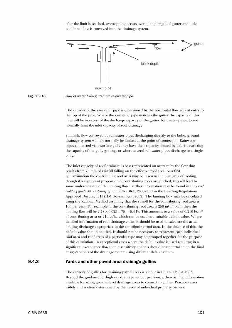
after the limit is reached, overtopping occurs over a long length of gutter and little

additional flow is conveyed into the drainage system.

Figure 9.10 Flow of water from gutter into rainwater pipe

The capacity of the rainwater pipe is determined by the horizontal flow area at entry to

the top of the pipe. Where the rainwater pipe matches the gutter the capacity of this

inlet will be in excess of the discharge capacity of the gutter. Rainwater pipes do not

normally limit the inlet capacity of roof drainage.

Similarly, flow conveyed by rainwater pipes discharging directly to the below ground

drainage system will not normally be limited at the point of connection. Rainwater

pipes connected via a surface gully may have their capacity limited by debris restricting

the capacity of the gully gratings or where several rainwater pipes discharge to a single

gully.

The inlet capacity of roof drainage is best represented on average by the flow that

results from 75 mm of rainfall falling on the effective roof area. As a first

approximation the contributing roof area may be taken as the plan area of roofing,

though if a significant proportion of contributing roofs are pitched, this will lead to

some underestimate of the limiting flow. Further information may be found in the Good

building guide 38: Disposing of rainwater (BRE, 2000) and in the Building Regulations

Approved Document H (HM Government, 2002). The limiting flow may be calculated

using the Rational Method assuming that the runoff for the contributing roof area is

100 per cent. For example, if the contributing roof area is 250 m² in plan, then the

limiting flow will be 2.78 × 0.025 × 75 = 5.4 l/s. This amounts to a value of 0.216 l/s/m²

of contributing area or 216 l/s/ha which can be used as a suitable default value. Where

detailed information of roof drainage exists, it should be used to calculate the actual

limiting discharge appropriate to the contributing roof area. In the absence of this, the

default value should be used. It should not be necessary to represent each individual

roof area and roof areas of a particular type may be grouped together for the purpose

of this calculation. In exceptional cases where the default value is used resulting in a

significant exceedance flow then a sensitivity analysis should be undertaken on the final

design/analysis of the drainage system using different default values.

9.4.3 Yards and other paved area drainage gullies

The capacity of gullies for draining paved areas is set out in BS EN 1253-1:2003.

Beyond the guidance for highway drainage set out previously, there is little information

available for sizing ground level drainage areas to connect to gullies. Practice varies

widely and is often determined by the needs of individual property owners.

CIRIA C635 101

For car parks, access roads and other areas drained by gullies, it is suggested that the

same principles are applied as for highway gullies (see Section 9.4.1). Data for the

hydraulic performance of slot drainage systems for exceedance conditions is not available.

It is possible that lack of maintenance will cause the slots to block thus limiting inlet flow.

However, in common with other drainage inlets, the capacity of such systems when clean

is normally in excess of the required inlet capacity. It is more probable that the actual

limit on inlet flow will occur at the connection to the underground pipe system. It should

be assumed that the limit on inlet capacity is similar to that which occurs with a gully inlet

system.

For smaller domestic areas such as yards and drives the situation is likely to be far more

variable. These gullies are also known to be badly maintained and gully pots are

sometimes broken. There is no known data available for establishing guidance for

calculating limiting flows. However, in the Building Regulations Approved Document

H (HM Government, 2002) recommends the use of 50 mm/hr for design. This equates

to 139l/s/ha of flow, and it is recommended that this be used as the limiting inlet

capacity for yard drainage. As this value is significantly less than that for highway

drainage, the consequence of this is that exceedance flow from yard drainage may be

localised, with the excess flow draining to a local highway drain during extreme events.

If the default values recommended above result in a significant exceedance flow then a

sensitivity analysis should be undertaken on the final design/analysis of the drainage

system using different default values.

9.4.4 Applying limiting inlet capacity to calculate exceedance flows

From the preceding sections it can be seen that for practical purposes the limitation of

inlet capacity to the drainage system can be expressed in terms of either a limiting

rainfall intensity or a limiting discharge per unit area. The procedure for determining

the division between minor system flow and major system flow (exceedance) is as

follows:

1 For each contributing area, divide the area up into different types eg roads, car

parks, roofs, paved areas, permeable areas.

2 For each type determine a suitable limiting discharge per unit area.

3 Group together areas sharing the same unit limiting discharge.

4 Identify each group as separate contributing areas in the drainage network model.

Depending on the software used this may require the specification of a separate

node for each group to connect to. These nodes should be joined together with

dummy pipes.

5 For each group, calculate the limiting discharge in l/s. This should be done by

multiplying the contributing area for the group by the corresponding unit limiting

discharge. For example if roof and yard areas combine to a total group area of

0.02 ha, then the limiting discharge will be 0.02 × 216 = 4.32 l/s using the default

value.

6 Apply this limiting discharge to the outlet from the connecting node in the model.

How this is done will depend on the software simulation tool used. Where the

software requires this to be specified as a whole number, the value should be

rounded down.

CIRIA C635102

9.5 Inlet capacity of SuDS systems

Where SuDS receive inflows from an upstream piped system, the inlet capacity will be

determined by the inlet capacity of the piped drainage system, as described earlier.

SuDS units falling into this category includes soakaways, storage ponds and basins.

Other SuDS, however, receive surface runoff directly. These include swales, infiltration

trenches and pervious pavements. Filter strips and green roofs fall into this category

but they are currently rare in the UK.

When SuDS receive runoff directly, the capacity will be limited by either the inflow, or

by the volume of storage. For example, the inlet capacity of a pervious pavement will

be exceeded when the rainfall intensity exceeds the capacity of the permeable surfacing

or when the storage capacity is exceeded. The latter will be depend on exfiltration or

outflow rate.

The inlet capacity of a particular SuDS unit will depend on the characteristics of the

rainfall, the contributing area and the SuDS unit itself. It can only be fully assessed by

detailed analysis or modelling. However, this will not be feasible at outline design stage

and may not be cost effective at detailed design.

To assist the designer a generic analysis of pervious pavements, swales and infiltration

trenches has been undertaken on a number of “standard sized” units, each draining a

unit contributing area of one hectare. Details of the analysis and further results are

given in Appendix 5 and the results are shown in Table 9.1 to 9.8. Results are quoted

separately for the south and the north of England to allow for difference in climate.

Values may be interpolated for intermediate locations.

Table 9.1 Overflow rate (l/s) from pervious pavement system – south

CIRIA C635 103

Additional paved area

(ha)0 1 2

Limiting discharge

rate l/s

Return period

1 2 5 10 1 2 5 10 1 2 5 10

1 0 0 0 0 0 0 0 0 0 0 0 0

10 0 0 0 0 0 0 0 0 0 0 0 0

30 0 0 0 0 0 0 0 0 0 0 0 0

100 0 0 0 0 0 0 0 0 27.1 25.7 22.0 7.826

200 0 0 0 0 4.4 3.1 0.0 0 44.6 43.2 39.4 33.6

Table 9.2 Overflow rate (l/s) from pervious pavement system – north

Table 9.3 Overflow volume (m³) from pervious pavement system – south

Table 9.4 Overflow volume (m³) from pervious pavement system – north

Table 9.5 Overflow rate (l/s) from 100m long swale system – south

CIRIA C635104


(ha)0 1 2

Limiting discharge

rate l/s

Return period

1 2 5 10 1 2 5 10 1 2 5 10

1 0 0 0 0 0 0 0 0 0 0 0 0

10 0 0 0 0 0 0 0 0 0 0 0 0

30 0 0 0 0 0 0 0 0 0 0 0 0

100 0 0 0 0 0 0 0 0 684.6 616.2 464.8 287.3

200 0 0 0 0 103.1 56.2 12 0 1116 1044 878.3 674.7


(ha)0 1 2

Limiting discharge

rate l/s

Return period

1 2 5 10 1 2 5 10 1 2 5 10

1 0 0 0 0 0 0 0 0 0 0 0 0

10 0 0 0 0 0 0 0 0 0 0 0 0

30 0 0 0 0 0 0 0 0 18.9 17.5 13.7 7.8

100 0 0 0 0 11.7 10.3 6.3 0.8 57.2 55.8 51.9 46.0

200 0 0 0 0 24.1 22.7 18.9 13.0 80.1 78.7 74.8 68.8


(ha)0 1 2

Limiting discharge

rate l/s

Return period

1 2 5 10 1 2 5 10 1 2 5 10

1 0 0 0 0 0 0 0 0 0 0 0 0

10 0 0 0 0 0 0 0 0 0 0 0 0

30 0 0 0 0 0 0 0 0 466 366 262 111

100 0 0 0 0 283 222 101 5.5 1401 1315 1155 940

200 0 0 0 0 610 542 391 219 1899 1810 1642 1413

Swale outflow rate (l/s) 0 1 2

Gradient (m/m)

Return period

0.05 0.02 0.01 0.004 0.05 0.02 0.01 0.004 0.05 0.02 0.01 0.004

1 0 0 0 0 0 0 0 0 2.7 0.8 0 0

10 0 0 0 0 0 0 0 0 14.4 5.6 1.1 0

30 0 0 0 0 6.5 0 0 0 27.0 14.3 3.5 0

100 15.4 0 0 0 31.7 8.7 0 0 44.5 30.8 11.8 0.6

200 29.3 0 0 0 41.0 20.9 0 0 51.4 39.8 18.8 1.7

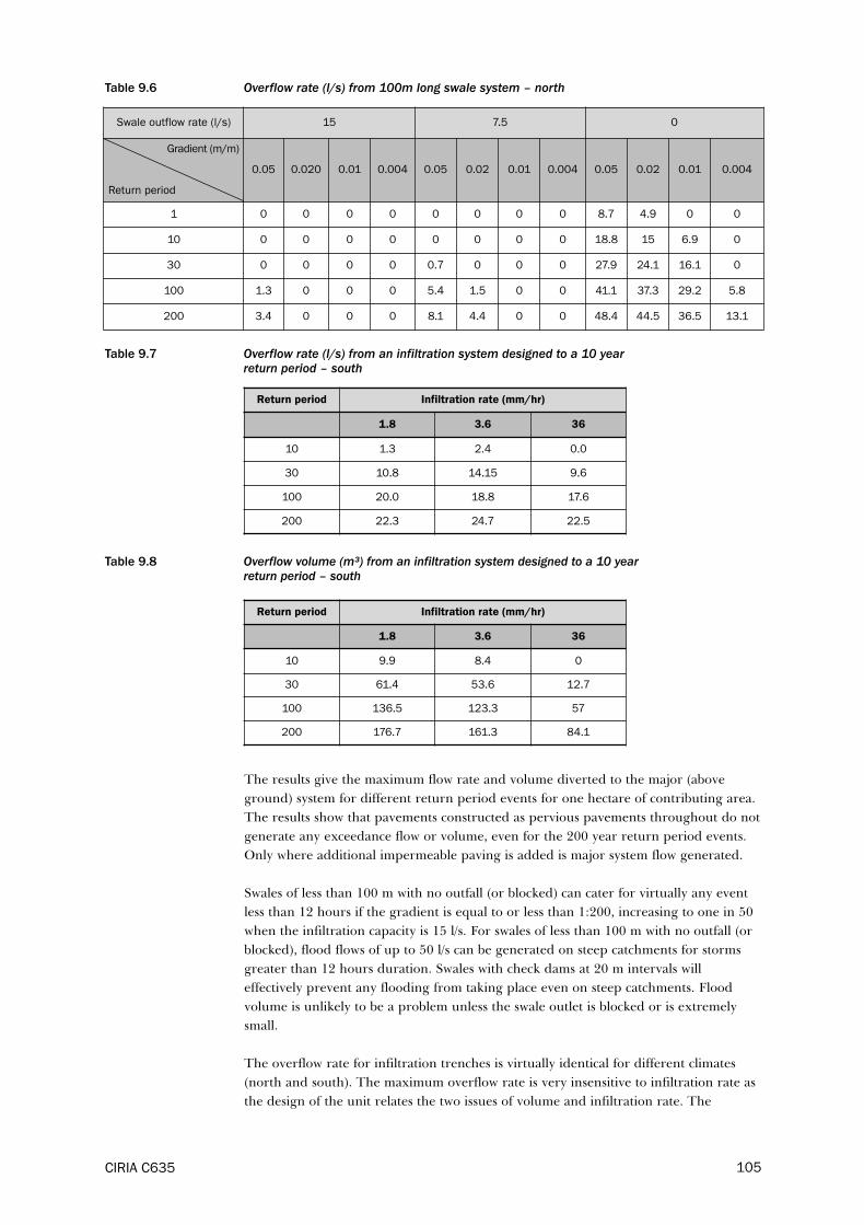
CIRIA C635 105

Table 9.6 Overflow rate (l/s) from 100m long swale system – north

Table 9.7 Overflow rate (l/s) from an infiltration system designed to a 10 yearreturn period – south

Table 9.8 Overflow volume (m³) from an infiltration system designed to a 10 yearreturn period – south

The results give the maximum flow rate and volume diverted to the major (above

ground) system for different return period events for one hectare of contributing area.

The results show that pavements constructed as pervious pavements throughout do not

generate any exceedance flow or volume, even for the 200 year return period events.

Only where additional impermeable paving is added is major system flow generated.

Swales of less than 100 m with no outfall (or blocked) can cater for virtually any event

less than 12 hours if the gradient is equal to or less than 1:200, increasing to one in 50

when the infiltration capacity is 15 l/s. For swales of less than 100 m with no outfall (or

blocked), flood flows of up to 50 l/s can be generated on steep catchments for storms

greater than 12 hours duration. Swales with check dams at 20 m intervals will

effectively prevent any flooding from taking place even on steep catchments. Flood

volume is unlikely to be a problem unless the swale outlet is blocked or is extremely

small.

The overflow rate for infiltration trenches is virtually identical for different climates

(north and south). The maximum overflow rate is very insensitive to infiltration rate as

the design of the unit relates the two issues of volume and infiltration rate. The

Return period Infiltration rate (mm/hr)

1.8 3.6 36

10 1.3 2.4 0.0

30 10.8 14.15 9.6

100 20.0 18.8 17.6

200 22.3 24.7 22.5

Return period Infiltration rate (mm/hr)

1.8 3.6 36

10 9.9 8.4 0

30 61.4 53.6 12.7

100 136.5 123.3 57

200 176.7 161.3 84.1

Swale outflow rate (l/s) 15 7.5 0

Gradient (m/m)

Return period

0.05 0.020 0.01 0.004 0.05 0.02 0.01 0.004 0.05 0.02 0.01 0.004

1 0 0 0 0 0 0 0 0 8.7 4.9 0 0

10 0 0 0 0 0 0 0 0 18.8 15 6.9 0

30 0 0 0 0 0.7 0 0 0 27.9 24.1 16.1 0

100 1.3 0 0 0 5.4 1.5 0 0 41.1 37.3 29.2 5.8

200 3.4 0 0 0 8.1 4.4 0 0 48.4 44.5 36.5 13.1

maximum overflow volumes are more sensitive to infiltration rate and climate with the

northern climate causing greater flooding. The maximum flood volume per house for a

200 year return period event is 5 m³

The designer may use Tables 9.1 to 9.8 to estimate exceedance flow and volumes for

outline design. At detailed design stage the designer should compare the details of the

proposed design with the “standard” arrangements used in the analysis, as summarised

in Appendix 5. Where the design differs significantly from these, the exceedance flow

and volume should be determined using the method set out in Appendix 6 or by using

the appropriate network model.

An example of using the graphs for a permeable pavement design are provided in

Appendix 7.

CIRIA C635106

10 Developing a risk assessment

10.1 An introduction to exceedance flood risk assessment

Assessing the risk of flooding to human life and property is very important. Flooding

has the potential to cause serious harm or death to human life or can have serious

socio-economic, financial and psychological effects. Surface flooding may be considered

in the very least to be inconvenient, however if flood water enters the property, then

significant damage can be caused to the internal fabric and fittings. Post flooding, a

substantial clean up operation is usually required to restore the property and its

contents to its former state. The ultimate cost of this clean up is passed back to

individual property owners or their insurers.

Assessing flood risk has become an important process. For example, the EA (Murphy,

2003) have adopted a more strategic approach by focusing on flood risk reduction

rather then just on flood defence. CIRIA C624 Development and flood risk – guidance for

the construction industry (Lancaster et al, 2004) provides a method to address flood risk as

part of the planning process. Other documents such as Sewers for adoption 5th edition

(Water UK and WRc, 2001) clearly highlight the need to understand what happens

with exceedance flow during extreme events.

Flood risk can be assessed by calculating the probability of an event occurring and the

subsequent impact that it has on a receptor. It is essential to consider risk in terms of

probability and consequence rather than one of these components in isolation. A

common misinterpretation of risk is that it is the probability of an event occurring only,

yet the consequences as a result of the event are just as important. For example,

flooding may regularly occur in a given location (hence having a high probability) but

the consequence of this flooding may be very limited so that the overall risk would be

low. Alternatively flood impact could be quite high, but the likelihood of such flooding

is so small that the overall risk is considered to be low. The following sections on

exceedance flood risk assessment (EFRA) will help to quantify this and offer principles

and methods that enable the user to determine a risk value. This flood risk assessment

guidance has been developed to apply to exceedance flooding from urban sewerage

systems, rather than other forms such as fluvial flooding.

10.2 Components of the EFRA

Many different components need to be considered when assessing exceedance flood

risk. Some of these are critical to quantifying risk, while other (softer) components such

as social, health and psychological impacts are less easy to quantify. Nevertheless, these

are important and a summary of their impact is included in this guidance. Currently

further research is required to quantify their effect (Evans et al, 2004).

CIRIA C635 107

The key components in the exceedance and flood risk assessment related to probability

and consequence are shown diagrammatically in Figure 10.1. In determining risk there

are three component groupings:

� inputs

� processes

� outputs.

There are three main groups of inputs that feed into the processes. Firstly there is the

determination of the exceedance flow, depth, velocity, volume and duration. This may

be determined through catchment modelling involving the use of computer simulation

models or hand calculations in the simple cases. The information contained in Chapters

6, 7 and 8 should be used to identify the most appropriate method for arriving at these

values. These will usually be determined for a particular rainfall return period,

specifying the probability of occurrence.

The second group of inputs that feed into the consequence part of the assessment are

measurable, and include damage to property or the health and safety of the public.

The third group are those which are more difficult to quantify and include the

environmental, socio-economic impacts and loss of facility.

Figure 10.1 Summary of the inputs, processes and outputs in the exceedance flood risk assessment

10.3 Determining the risk value

10.3.1 EFRA process

The process to determine the risk is illustrated in the two flowcharts in Figures 10.2

and 10.3 and is divided into two parts. The level of detail used in the risk assessment

should match the level of detail of the study, as set out in Box 9.1. This is discussed

further in Section 10.3.

CIRIA C635108

Catchment

modelling

Exceedance

flow/volume

Social

factors

Environmental

Loss of

facility

Damage cost

Health

and safety

Probability

Input ProcessKey:

Consequence

Output

Risk

The following sections describe each step of the process in detail.

Step 1: Determine the level of risk assessment using the criteria set out in Box 9.1.

Step 2: This involves selecting the critical (worst case) duration for the rainfall event

used in the assessment. When using the Rational Method (level 1 studies only, see

Appendix G) the critical duration should be equal to the time of concentration for the

drainage area and this value should be used for all storm return periods. If a hydraulic

computer simulation tool is used then 30 year return period design events should be

selected and run with the hydraulic model (can be used for all levels of study). The

critical duration can then be determined from the storm that creates the most

significant flooding or highest surcharge levels.

Step 3: The 30 year return period design storm is used to initially identify if flooding

occurs and the location. The method of calculation (or modelling) will be determined

by the level of study (level of risk assessment) as set out in Box 9.1 and discussed in

Section 10.3 below. If no flooding occurs in the area, then the return period is

increased appropriately, until flooding appears.

Step 4: This step involves calculating the consequence of any flooding. The level of

detail used in the calculation and in quantifying consequence will again depend on the

level of risk assessment being used (see Section 10.3). Once the consequence has been

determined, this is combined with probability (obtained from the rainfall return period)

to determine the risk score (using the risk matrix in Figure 10.4).

Step 5: If necessary the process may be repeated for other return period events.

Revising the assessment with a storm of higher or lower return period should be

determined by the level of flooding and risk from the previous assessment. It is

expected that the risk rating determined for a range of storms is unlikely to increase or

decrease by more than one value. If a wide range of values is obtained, this will indicate

that the area may be sensitive to minor changes or that some of the input values may

be incorrect.

CIRIA C635 109

Level 1

Rational Method

Determine

time of

concentration

Run 30 or 100 year return

period storms with different

durations

Identify the worst

storm for flooding/

surcharge level

Determine

the critical

duration

Level 1, 2 or 3

Hydraulic

simulation model

STE

P 1

STE

P 2

Figure 10.2 Part 1 Generic EFRA process to determine the critical duration for the area being assessed

CIRIA C635110

to Figure 10.3

Catchment size

and complexity

Select

EFRA level

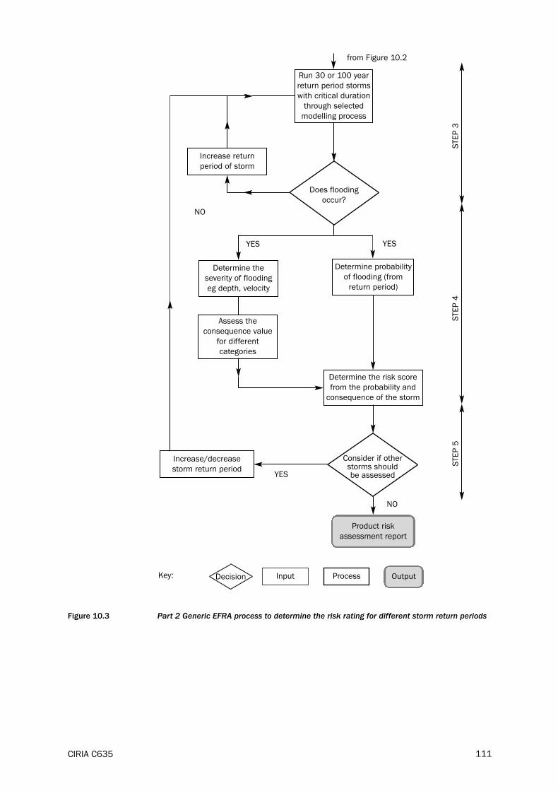
Figure 10.3 Part 2 Generic EFRA process to determine the risk rating for different storm return periods

CIRIA C635 111

Increase return

period of storm

Determine the risk score

from the probability and

consequence of the storm

Determine probability

of flooding (from

return period)

from Figure 10.2

NO

YES YES

YES

NO

STE

P 5

STE

P 4

STE

P 3

Determine the

severity of flooding

eg depth, velocity

Assess the

consequence value

for different

categories

Run 30 or 100 year

return period storms

with critical duration

through selected

modelling process

Increase/decrease

storm return period

Consider if otherstorms shouldbe assessed

Decision

Does flooding

occur?

Input ProcessKey: Output

Product risk

assessment report

Figure 10.4 Showing the risk value depend on the probability and consequence value determined.Note: This figure is only indicative, and the scoring of probability and consequence, and risk should be adjusted to suit

particular circumstances

10.3.2 Selection of the appropriate EFRA level

Any risk assessment undertaken should be appropriate to the size and complexity of

the area being assessed. The EFRA has been split into three levels, and relates to the

three levels of study discussed in Section 9.2. A level 1 study will be applicable to small

drainage areas that have a simple dendritic drainage layout without complex

ancillaries. A level 2 study will be applicable to large or complex drainage systems. A

level 3 study will be applicable to large and complex drainage systems. The information

required to complete the different levels of EFRA are described in the following

sections.

An initial scoping study can be used to identify the appropriate extent and detail of the

final study. Scoping studies should be conducted as level 1 studies with consequence

assessed from Table 10.6. Further detail can then be added as necessary to build up the

study to level 2 or 3 in certain areas.

There are similarities in the information requirements to complete an EFRA for

existing and newly designed drainage systems. An existing system will make use of

current information. Any existing flooding data should be considered and used to

verify modelling and calculations produced to identify existing flood paths prior to

developing solutions. New designs will make use of development and works drawings.

The proposed information and the assessment could provide extra evidence to the

flood risks in any proposed development plan.

An example of undertaking a risk assessment at a variety of levels is considered in the

case study in Part D.

CIRIA C635112

10.3.3 Level 1 EFRA – simple small areas

Simple small areas are treated as having dendritic drainage layouts without complex

ancillaries. This level is applicable to property flooding rather than health and safety

risks. The various phases of the Level 1 EFRA is detailed in Table 10.1 which includes a

summary of the information, inputs and outputs (see Sections 9.2 and 9.3). In a level 1

study the minor system is ignored and all the flow is assumed to be conveyed by the

surface pathways. The surface pathways form the drainage network.

Table 10.1 Summary of the phases used to undertake each level of study

CIRIA C635 113

Phase Description

Level of study

1 2 3

Desktop study

Collect OS mapping/development plans.

Collect sewer system data/locations.

Collect topographical data (preferably in digital form).

Collect available information on previous flooding incidents (eg

photographs, videos).

Identify low spots (including location of properties with cellars).

Identify and map potential above ground flow paths.

Digitally map above ground flow paths.

Identify and map known/potential flooding locations.

Assess known flood paths if existing site to be re-developed.

�

�

�

�

�

�

�

�

�

�

�

�

�

�

�

�

�

�

�

�

On-site study Site visit to confirm desktop assessment. � � �

Flow calculation

Select an appropriate method for calculating surface runoff (Chapter 8).

Select appropriate rainfall return period (Chapter 6) and determine critical

duration (step 2 above).

Compute peak rate of runoff from contributing areas.

Calculate flows in surface flood pathways.

Take off contributing areas from mapping, taking care to include pervious

areas that drain to the system.

Select a suitable runoff model (Chapter 8).

Select suitable sewer network modelling software capable of replicating

surcharging and surface flooding.

Commission a short term flow survey to verify sewer model

(*large and more complex areas on level 2).

Add in surface pathways to model as appropriate.

Model above ground pathways.

Model inlet capacity and minor/major interaction.

Run model with different duration storms to determine the critical

duration.

�

�

�

�

�

�

�

�

�

�

�

�

�

�

�

�

�

Flooding location/

volume

Compare computed flows with capacity of surface flood pathways.

Identify flooding location and approximate volume.

Run model with appropriate return period to compute location and degree

of surface flooding.

Identify conveyance in surface pathways and locations and depths of

surface flooding.

Identify the depth and velocity in above ground flow paths.

Identify depth and velocity surrounding property.

�

�

�

�

�

�

�

�

10.3.4 Level 2 EFRA – large or complex areas

A level 2 study is appropriate for the analysis/design of medium to large or complex

systems (for further information see Section 9.2 and 9.3). In this study the minor

drainage system will be analysed/designed using sewer network modelling software

capable of replicating surcharging and surface flooding. Surface flooding is represented

by ponding in low spots, which are identified and sized by local interpretation or using

a topographical model. Surface conveyance is represented either by modelling surface

flood pathways explicitly, or by using a “rolling ball” software with a digital terrain

model. The drainage network may consist exclusively of the minor (below ground)

drainage network or a combination of minor and major drainage systems.

Contributing pervious areas are modelled in the sewer network model, however no

allowance is made for inlet capacity. The volume and depth of flooding is calculated but

the velocity of surface flow is not. A level 2 study is applicable in determining the risk of

property flooding based upon depth (Table 10.1).

10.3.5 Level 3 EFRA – large and complex areas

A level 3 study is appropriate for the design and analysis of large and complex

drainage systems (see Sections 9.2 and 9.3). The minor drainage system is analysed/

designed using sewer network modelling capable of replicating surcharging, backwater

effects and surface flooding. Surface conveyance is replicated by the explicit modelling

of known surface flood pathways with full interaction between the major and minor

networks. Contributing pervious areas are explicitly modelled and an allowance is

made for inlet capacity on an area or individual basis. A level 3 study enables the flood

risk on property (depth and velocity), loss of business and health and safety

consequences to be assessed (Table 10.1).

CIRIA C635114

Determine

probability

Identify the probability that a location will be flooded (Section 10.5).

Identify the likely flood depth banding that causes:

� basement flooding

� external flooding

� ground floor and above flooding.

Identify flood depth at locations with critical storm.

Identify internal flooding frequency.

�

�

�

�

�

�

�

�

Determine

consequence

Identify initial property consequence from Table 10.7.

Identify property type(s).

Determine adjusted consequence value based upon flood depth

banding.

Determine consequence rating dependent upon depth property depth

and adjusted for velocity.

Determine psychological consequence.

Determine loss of business consequence (if applicable).

Determine health and safety consequence.

�

�

�

�

�

�

�

�

�

Determine risk

Using the risk matrix (Figure 10.4), determine risk value for:

� groups of property

� individual property

� loss of business

� limited health and safety.

�

�

�

�

�

�

�

�

�

�

�

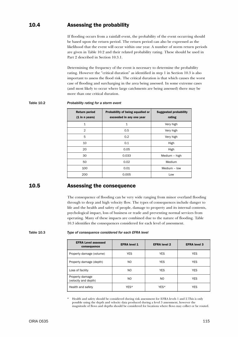
10.4 Assessing the probability

If flooding occurs from a rainfall event, the probability of the event occurring should

be based upon the return period. The return period can also be expressed as the

likelihood that the event will occur within one year. A number of storm return periods

are given in Table 10.2 and their related probability rating. These should be used in

Part 2 described in Section 10.3.1.

Determining the frequency of the event is necessary to determine the probability

rating. However the “critical duration” as identified in step 1 in Section 10.3 is also

important to assess the flood risk. The critical duration is that which causes the worst

case of flooding and surcharging in the area being assessed. In some extreme cases

(and most likely to occur where large catchments are being assessed) there may be

more than one critical duration.

Table 10.2 Probability rating for a storm event

10.5 Assessing the consequence

The consequence of flooding can be very wide ranging from minor overland flooding

through to deep and high velocity flow. The types of consequences include danger to

life and the health and safety of people, damage to property and its internal contents,

psychological impact, loss of business or trade and preventing normal services from

operating. Many of these impacts are combined due to the nature of flooding. Table

10.3 identifies the consequences considered for each level of assessment.

Table 10.3 Type of consequence considered for each EFRA level

* Health and safety should be considered during risk assessment for EFRA levels 1 and 2.This is onlypossible using the depth and velocity data produced during a level 3 assessment, however themagnitude of flows and depths should be considered for locations where flows may collect or be routed.

CIRIA C635 115

Return period

(1 in n years)

Probability of being equalled or

exceeded in any one year

Suggested probability

rating

1 1 Very high

2 0.5 Very high

5 0.2 Very high

10 0.1 High

20 0.05 High

30 0.033 Medium – high

50 0.02 Medium

100 0.01 Medium – low

200 0.005 Low

EFRA Level assessed

consequence EFRA level 1 EFRA level 2 EFRA level 3

Property damage (volume) YES YES YES

Property damage (depth) NO YES YES

Loss of facility NO YES YES

Property damage

(velocity and depth) NO NO YES

Health and safety YES* YES* YES

10.5.1 Consequence hierarchy for building types or land use as a result of

flooding

Damage to property is regularly reported by the media and can be a significant

consequence of flooding. Table 10.4 gives an initial indication of the consequence rating

for property flooding. It has been developed using information available in PPG 25,

and identifies a hierarchical approach to flooding. The table may be used in level 1

studies and as an initial assessment of risk in identifying appropriate levels of study.

Table 10.4 Initial hierarchy of the consequences of flooding certain properties/locations

10.5.2 Damage to property

Damage can be caused in the short term and the property will need to be dried out with

the contents replaced, refer to CIRIA C623 Standards for the repair of buildings following

flooding (Garvin et al, 2005). More severe flooding can cause long term structural damage

and this has more significant implications. An indication of the typical consequences as a

result of flooding to residential properties is described in Table 10.5. A number of

factors are involved in property flooding including the depth of water, duration of

flooding, wave effects, external pressures, velocity of the water and water quality.

The form of construction of a property can have an effect on the amount of damage

caused and this commented on further in Section 13.3.1.

CIRIA C635116

Potential impact zones or structures Initial consequence rating

� hospitals

� junior/infant school and nurseries

� senior citizen housing

� emergency services

� telecommunication centres

� high value manufacturing

� temporary domestic dwellings (mobile home/pre-fabs)

� major shopping areas

� any facilities located in a tunnel (London Underground, subways etc)

� major stormwater pumping stations

� power supplies

� water and wastewater treatment works

� road/railway cuttings

� underground car parks

� access for emergency services and to these areas.

High

� major highways/transport routes

� medium/low value manufacturing

� permanent domestic dwellings

� other schools

� commercial/business areas

� local shopping areas

� major sports facilities.

Medium

� playing fields and open space

� minor highways/transport routes

� car parks and minor sports facilities

� derelict buildings

� brownfield sites

� canals.

Low

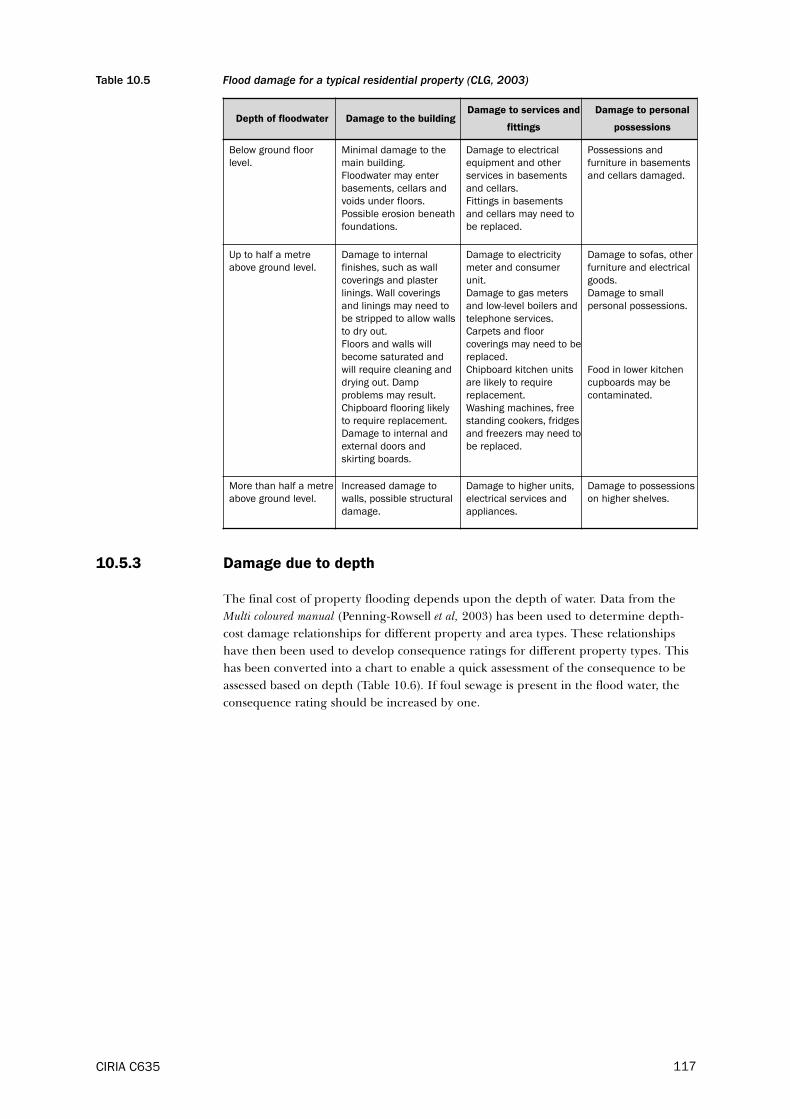
Table 10.5 Flood damage for a typical residential property (CLG, 2003)

10.5.3 Damage due to depth

The final cost of property flooding depends upon the depth of water. Data from the

Multi coloured manual (Penning-Rowsell et al, 2003) has been used to determine depth-

cost damage relationships for different property and area types. These relationships

have then been used to develop consequence ratings for different property types. This

has been converted into a chart to enable a quick assessment of the consequence to be

assessed based on depth (Table 10.6). If foul sewage is present in the flood water, the

consequence rating should be increased by one.

CIRIA C635 117

Depth of floodwater Damage to the buildingDamage to services and

fittings

Damage to personal

possessions

Below ground floor

level.

Minimal damage to the

main building.

Floodwater may enter

basements, cellars and

voids under floors.

Possible erosion beneath

foundations.

Damage to electrical

equipment and other

services in basements

and cellars.

Fittings in basements

and cellars may need to

be replaced.

Possessions and

furniture in basements

and cellars damaged.

Up to half a metre

above ground level.

Damage to internal

finishes, such as wall

coverings and plaster

linings. Wall coverings

and linings may need to

be stripped to allow walls

to dry out.

Floors and walls will

become saturated and

will require cleaning and

drying out. Damp

problems may result.

Chipboard flooring likely

to require replacement.

Damage to internal and

external doors and

skirting boards.

Damage to electricity

meter and consumer

unit.

Damage to gas meters

and low-level boilers and

telephone services.

Carpets and floor

coverings may need to be

replaced.

Chipboard kitchen units

are likely to require

replacement.

Washing machines, free

standing cookers, fridges

and freezers may need to

be replaced.

Damage to sofas, other

furniture and electrical

goods.

Damage to small

personal possessions.

Food in lower kitchen

cupboards may be

contaminated.

More than half a metre

above ground level.

Increased damage to

walls, possible structural

damage.

Damage to higher units,

electrical services and

appliances.

Damage to possessions

on higher shelves.

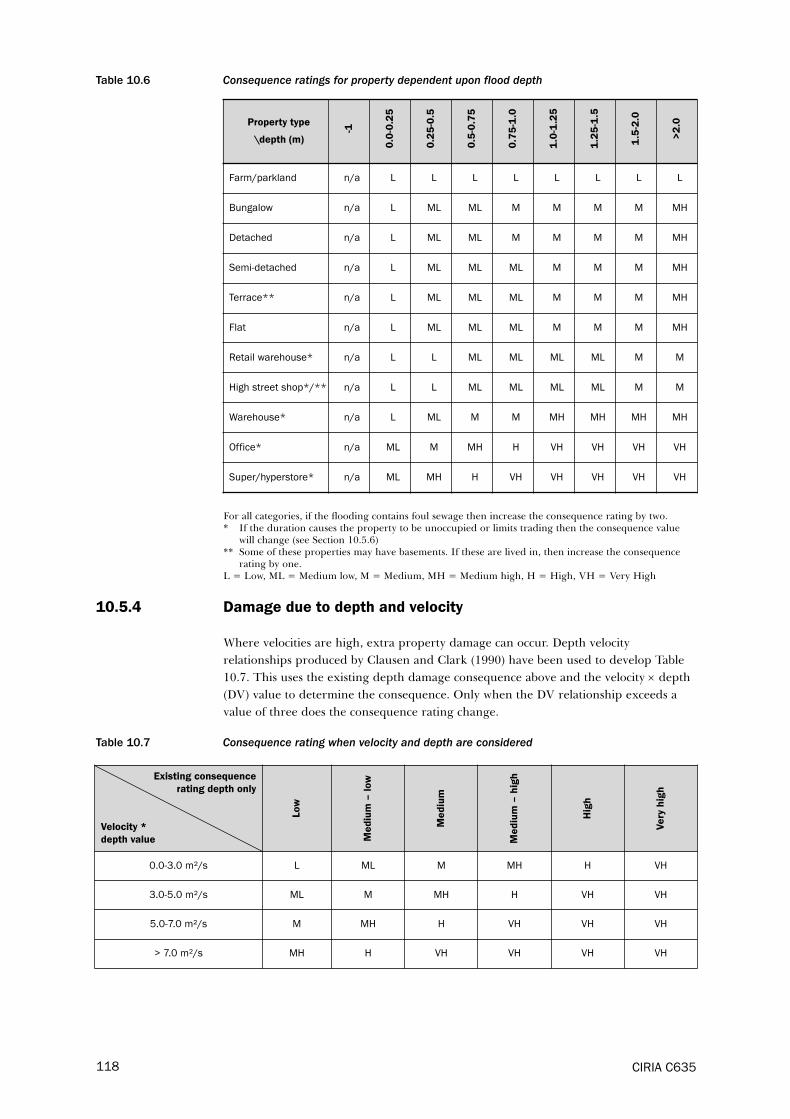
Table 10.6 Consequence ratings for property dependent upon flood depth

For all categories, if the flooding contains foul sewage then increase the consequence rating by two.* If the duration causes the property to be unoccupied or limits trading then the consequence value

will change (see Section 10.5.6)** Some of these properties may have basements. If these are lived in, then increase the consequence

rating by one.L = Low, ML = Medium low, M = Medium, MH = Medium high, H = High, VH = Very High

10.5.4 Damage due to depth and velocity

Where velocities are high, extra property damage can occur. Depth velocity

relationships produced by Clausen and Clark (1990) have been used to develop Table

10.7. This uses the existing depth damage consequence above and the velocity × depth

(DV) value to determine the consequence. Only when the DV relationship exceeds a

value of three does the consequence rating change.

Table 10.7 Consequence rating when velocity and depth are considered

CIRIA C635118

Existing consequence

rating depth only

Velocity *

depth value

Lo

w

Me

diu

m –

lo

w

Me

diu

m

Me

diu

m –

hig

h

Hig

h

Ve

ry h

igh

0.0-3.0 m²/s L ML M MH H VH

3.0-5.0 m²/s ML M MH H VH VH

5.0-7.0 m²/s M MH H VH VH VH

> 7.0 m²/s MH H VH VH VH VH

Property type

\depth (m)

-1

0.0

-0.2

5

0.2

5-0

.5

0.5

-0.7

5

0.7

5-1

.0

1.0

-1.2

5

1.2

5-1

.5

1.5

-2.0

>2

.0

Farm/parkland n/a L L L L L L L L

Bungalow n/a L ML ML M M M M MH

Detached n/a L ML ML M M M M MH

Semi-detached n/a L ML ML ML M M M MH

Terrace** n/a L ML ML ML M M M MH

Flat n/a L ML ML ML M M M MH

Retail warehouse* n/a L L ML ML ML ML M M

High street shop*/** n/a L L ML ML ML ML M M

Warehouse* n/a L ML M M MH MH MH MH

Office* n/a ML M MH H VH VH VH VH

Super/hyperstore* n/a ML MH H VH VH VH VH VH

10.5.5 Health and safety

Health and safety impacts are wide ranging and include:

� storm water mixed with foul sewage presenting a health risk

� pedestrians being at risk from drowning due to the depth of the flood water

� the combination of the depth and velocity could knock a pedestrian off their feet

� vehicles could be carried away by a combination of depth and velocity

� blown manhole covers leaving an exposed entry could become a trip or fall hazard

to pedestrians and vehicles.

When considering the consequence of the flow depth and velocity to pedestrians, the

following chart can be used to determine the consequence rating (Table 10.8). This is

based upon research undertaken by Helsinki University of Technology (2001) and

Defra/EA (Ramsbottom et al, 2003). The rating is dependent upon the depth of the DV

relationship and the external conditions. Three external conditions are considered and

the two extremes, good and bad are described in more detail in Table 10.9. Further

reading is available in reports on Flood Risk to People (Phase 1 and 2 of a Defra/EA

project) by Ramsbottom et al (2003) and HR Wallingford et al (2004).

When considering the consequence of the flow DV relationship to cars and their

passengers, Table 10.10 can be used to determine the consequence rating. This is based

upon research reported by Reiter (2000).

Table 10.8 Consequence rating for pedestrians in flood water. For children and the elderly, increase theconsequence rating by one

CIRIA C635 119

Surrounding conditions

Depth or depth*

velocity value

Good conditions Normal conditions Poor conditions

0.5 m L ML MH

1.0 m ML M H

0.5 m²/s M H VH

1.0 m²/s MH VH VH

1.5 m²/s H VH VH

> 1.5 m²/s VH VH VH

Table 10.9 Description of the two condition extremes for pedestrians

Table 10.10 Consequence rating for humans in cars and damage to the car itself

10.5.6 Loss of facility/business

Loss of facility occurs when flooding limits or prevents a service or function from

operating correctly and is likely to have an economic impact. This could be, for

example, if a shop is flooded and limits or prevents customers entering. Alternatively,

electricity supplies could be stopped which can cause further impacts beyond the

immediate area of flooding. However the cost of this can be estimated.

Financial implications from the interruption is very important and could cause a

company to cease trading due to loss of custom in the short or long term. If the

duration causes the property to be unoccupied or limits trading the consequence rating

identified in Table 10.8 should be increased by one. If the duration causes the property

to cease trading for a considerable period of time, the consequence rating should be

increased by two.

10.5.7 Emergency services

Some areas have higher consequences as a result of flooding compared with others and

they should be protected from “any conceivable event”. These would include, for

example, the headquarters and depots of emergency services, high security installations

and certain medical facilities. This classification should be used sparingly. For practical

purposes “any conceivable event” may be interpreted as the 1000 year event.

CIRIA C635120

Conditions

Criteria

Good Poor

Ground surface Smooth, not slippery and no obstacles Uneven, slippery, obstacles

Water No moving debris, warm, good visibility Moving debris, low temperature, poor visibility

Human subjectNot carrying any additional load, in good

health

Carrying additional load, disabled, elderly or a

child

Lighting Good lighting, daylight Poor lighting, night time

Criteria

Depth × velocity range

Damage to car Adult in a car Child in a car

ML M H

< 0.1 m²/s L L L

0.1 – 0.3 m²/s L LM M

0.3 – 0.6 m²/s M M H

> 0.6 m²/s H VH VH

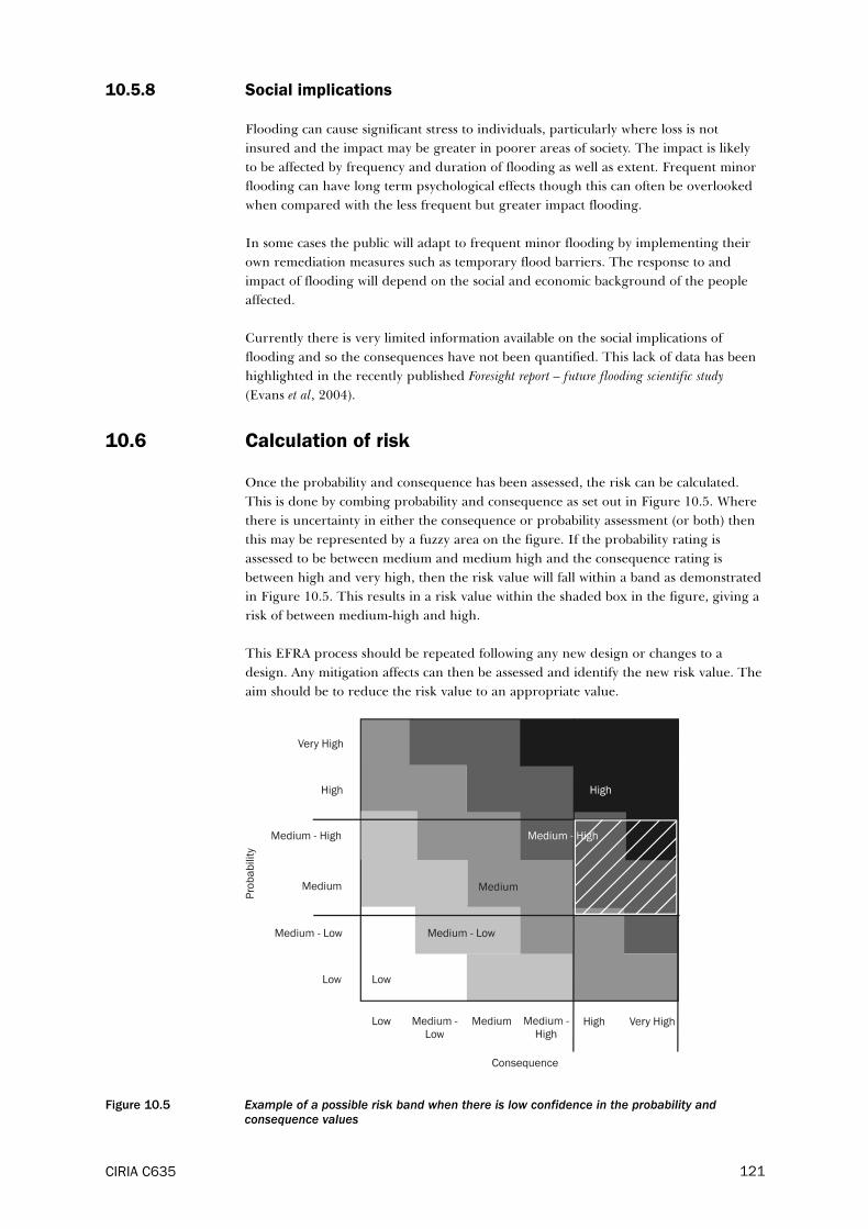
10.5.8 Social implications

Flooding can cause significant stress to individuals, particularly where loss is not

insured and the impact may be greater in poorer areas of society. The impact is likely

to be affected by frequency and duration of flooding as well as extent. Frequent minor

flooding can have long term psychological effects though this can often be overlooked

when compared with the less frequent but greater impact flooding.

In some cases the public will adapt to frequent minor flooding by implementing their

own remediation measures such as temporary flood barriers. The response to and

impact of flooding will depend on the social and economic background of the people

affected.

Currently there is very limited information available on the social implications of

flooding and so the consequences have not been quantified. This lack of data has been

highlighted in the recently published Foresight report – future flooding scientific study

(Evans et al, 2004).

10.6 Calculation of risk

Once the probability and consequence has been assessed, the risk can be calculated.

This is done by combing probability and consequence as set out in Figure 10.5. Where

there is uncertainty in either the consequence or probability assessment (or both) then

this may be represented by a fuzzy area on the figure. If the probability rating is

assessed to be between medium and medium high and the consequence rating is

between high and very high, then the risk value will fall within a band as demonstrated

in Figure 10.5. This results in a risk value within the shaded box in the figure, giving a

risk of between medium-high and high.

This EFRA process should be repeated following any new design or changes to a

design. Any mitigation affects can then be assessed and identify the new risk value. The

aim should be to reduce the risk value to an appropriate value.

Figure 10.5 Example of a possible risk band when there is low confidence in the probability andconsequence values

CIRIA C635 121

CIRIA C635122

11 Designing for surface conveyance

11.1 Principles of design

This chapter looks in detail at how surface channels for flood conveyance may be

specifically accommodated in new and existing development, and how they should be

designed to convey the exceedance flow. It also deals with some of the health and safety

issues raised in Chapter 10.

Channels designed to function as surface flood pathways during extreme events may,

on a day to day basis, serve as:

� highways

� footpaths

� ditches and swales

� car parks

� vegetated channels formed naturally or artificially.

The main use of such pathways is referred to as the primary function, with flood

conveyance becoming the secondary function. In exceptional circumstances pathways

may be defined where flood conveyance is the primary function.

When designing surface flood pathways for extreme events, the engineer should be

aware of the primary function of the proposed pathway. Engineers should not

compromise the primary function and due care should be taken of the safety

implications of infrequent flooding of a facility normally used for another purpose. For

example, the risk of drowning in areas that only occasionally flood may be greater than

in areas where water is retained permanently. An integrated approach is required when

planning and designing surface flood pathways with building position and street

furniture, to prevent flooding caused by such obstacles. This is discussed further in

Chapter 13.

Surface flood channels for extreme events should:

� not detract from the primary function except during extreme events

� convey the required exceedance flow

� provide a freeboard to allow for wave action and any uncertainties in design

� limit the depths and velocities so as not to pose undue risk to the primary function,

property or the public

� provide a smooth transition from the primary to secondary function and back, ie

sudden rises in flood flow/depth/velocity should be avoided

� minimise the possibility of sediments or trash accumulated during extreme events

to hinder the proper operation of the flood pathway

� not intercept or block pathways that the public may need to use to escape from

flooded areas.

Figure 11.1 shows the inputs, processes and outputs involved in designing the surface

flood pathways for conveyance. Figure 11.2 sets out the design procedure in a

CIRIA C635 123

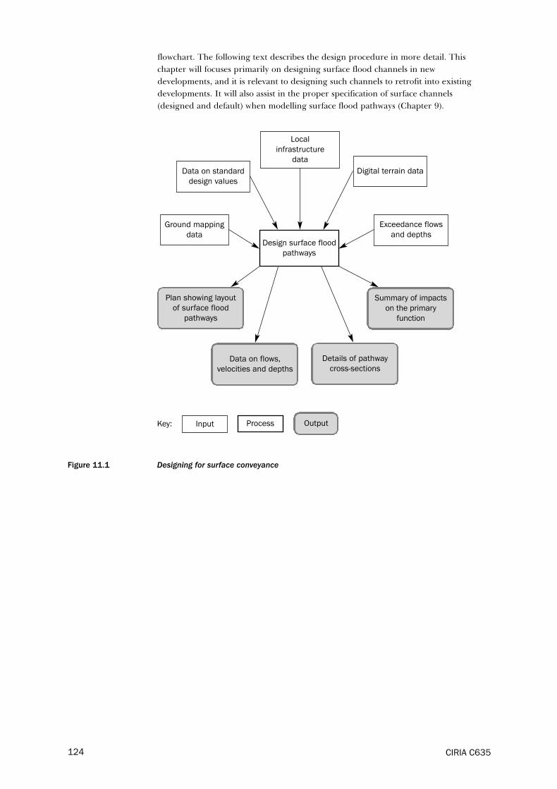
flowchart. The following text describes the design procedure in more detail. This

chapter will focuses primarily on designing surface flood channels in new

developments, and it is relevant to designing such channels to retrofit into existing

developments. It will also assist in the proper specification of surface channels

(designed and default) when modelling surface flood pathways (Chapter 9).

Figure 11.1 Designing for surface conveyance

Data on flows,

velocities and depths

Output

CIRIA C635124

Data on standard

design values

Ground mapping

dataDesign surface flood

pathways

Digital terrain data

Exceedance flows

and depths

Local

infrastructure

data

Input ProcessKey:

Details of pathway

cross-sections

Plan showing layout

of surface flood

pathways

Summary of impacts

on the primary

function

CIRIA C635 125

Is a digital

terrain model

available?

Figure 11.2 Flowchart for designing surface flood channels for extreme events

Use contour map and site

inspection to identify

default pathways

YES

YES

NO

NO

Modify default pathway

layout to identify

designed pathway layout

Divide pathways into

reaches of about

constant cross-section

and slope

Review highway

layout etc and modify

default pathways

Use DTM and rolling

ball model to identify

default pathways

Have default

flood pathways

been identified?

Collect terrain data

and mapping

CIRIA C635126

Figure 11.2 (cont’d) Flowchart for designing surface flood channels for extreme events

Assign exceedance flows to

each pathway from previous

computations

Calculate velocities and depth

in each reach including

allowance for freeboard

Check conditions

at transitions

Review results Review results

Decision

Revise model to include

designed pathways and

re-run with extreme events

Check flow balance at

transitions and match with

total exceedance flows

Is the model of

the above ground

flood paths

available?

Modify channel sections/

transitions to meet

requirements of flow,

velocity and depth

OutputInput ProcessKey:

Report

11.2 Identifying flood pathways

On undeveloped sites, natural drainage channels are defined by topography, with water

draining to low spots and being conveyed at the bottom of natural valleys. The use of

DTMs can aid the identification of existing flood pathways in undeveloped areas. When

developing greenfield sites, designed surface flood channels can be most effective when

they follow the natural drainage paths. Since these may differ considerably from the

infrastructure layout of the proposed development, early consideration of exceedance

conveyance in the planning process is desirable.

On developed sites, retrofitting surface flood channels can prove more difficult, with

the engineer largely being restricted to adapting existing highways, paths and spaces

between buildings. In either case, building layout, road design and other barriers or

channels will influence the resulting network of surface flood pathways. This is dealt

with in more detail in Chapter 13.

Where exceedance flows have been calculated using a drainage network model, an

initial assessment of flood pathways (default pathways) will have been made. When

designing new or modified surface flood pathways, the layout and cross-sections should

be based initially on these assessments. It may be necessary to make changes to the

direction and capacity of pathways in order to provide the desired level of protection to

property and the public (ie reducing the flood risk to a desirable level). This may result

in the identification, and subsequent modification and construction of new flood

pathways and the abandonment of some default pathways.

Where default flood pathways have not been previously identified, an initial assessment

of the site should be made. This should include a review of the topography of the site,

and if digital terrain data is available, a rolling ball model can be used to make an initial

assessment. However, flood pathways may be extensively modified by highway layout,

paths and other artificial landscape features, and default pathways should account for

this. Ideally these will have been confirmed by observation during wet weather and

through meetings with local residents.

11.3 Designing flood channels

11.3.1 Channel conveyance

The channel forming the flood pathway may be designed using the Manning Equation

set out in Equation 9.3. This equation is based on the assumption that uniform flow

occurs in the channel. This requires a constant cross-section, surface roughness and

slope. In practice all three of these will vary somewhat, and average values have to be

used. However there will be cases where significant changes in any of these variables

make an averaging process inappropriate. An example would be a significant change in

channel slope, such as occurs when a road changes direction from running with the

contours to cross them. Before calculating channel capacity the design surface flood

channels should be divided into separate reaches where the cross-section, surface

roughness and slope can be considered to be sensibly uniform.

CIRIA C635 127

(9.3)

where:

Q = discharge, m³/s

n = Manning roughness value

R = hydraulic radius = A/P

s = slope (decimal)

AC = cross-sectional area of flow, m²

P = wetted perimeter, m

The exceedance flow to be conveyed is represented by the discharge Q. For a given

cross-section shape, the depth is determined using Equation 9.3. The equation is solved

by trial and error (ie various depths are chosen), the corresponding section properties

calculated, and the discharge determined. This is repeated until the discharge

calculated matches the exceedance flow to be conveyed.

When using the Manning Equation the roughness value n should be chosen with care.

Typical values of n for different types of channel surface are given in Table 11.1.

Table 11.1 Values of Manning roughness coefficient ‘n’ for use with Equation 9.3

Note: When choosing an appropriate n value the engineer should assess the smoothness of surfacefinish against the norm that can be expected for the surface type, using higher n values forrougher finishes. For grass lined channels the lower values refer to rye grass and the highervalues to fescues (Chow, 1959; Escarameia and May, 1996; Escarameia et al, 2002).

Calculated depths may also be affected by local disturbances. Evidence suggests that

flood flow depths temporarily increase significantly due to wave action from moving

vehicles for example (Figure. 11.3). The calculation of conveyance capacity also carries

a significant amount of uncertainty and when designing flood channels, the engineer

should include some freeboard to allow for these factors. Freeboard equal to 25 per

cent of the required flood depth is considered to be reasonable. If the flood pathway is

contained entirely within a highway bounded by 100 mm kerbs, the maximum design

depth of flow would be 80 mm. Even with this allowance, occasional overtopping of the

channel due to flood waves from moving vehicles can be expected. Where this is likely

to cause a significant increase in flood risk (such as where property doorways open

CIRIA C635128

Surface type n

Rough concrete (unfinished) 0.014 – 0.020

Smooth concrete (float or slip formed finish) 0.009 – 0.020

Paving flags (well laid with mortar joints) 0.015 – 0.020

Hot rolled asphalt 0.013 – 0.016

Surfaced dressed 0.017 – 0.025

Well formed setts 0.018 – 0.030

Mowed grass (in artificial grass lined drainage channels) 0.057 – 0.061

Unmown grass (artificial grass lined drainage channels) 0.067 – 0.083

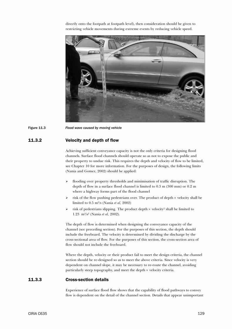
directly onto the footpath at footpath level), then consideration should be given to

restricting vehicle movements during extreme events by reducing vehicle speed.

Figure 11.3 Flood wave caused by moving vehicle

11.3.2 Velocity and depth of flow

Achieving sufficient conveyance capacity is not the only criteria for designing flood

channels. Surface flood channels should operate so as not to expose the public and

their property to undue risk. This requires the depth and velocity of flow to be limited,

see Chapter 10 for more information. For the purposes of design, the following limits

(Nania and Gomez, 2002) should be applied:

� flooding over property thresholds and minimisation of traffic disruption. The

depth of flow in a surface flood channel is limited to 0.3 m (300 mm) or 0.2 m

where a highway forms part of the flood channel

� risk of the flow pushing pedestrians over. The product of depth × velocity shall be

limited to 0.5 m²/s (Nania et al, 2002)

� risk of pedestrians slipping. The product depth × velocity² shall be limited to

1.23 m³/s² (Nania et al, 2002).

The depth of flow is determined when designing the conveyance capacity of the

channel (see preceding section). For the purposes of this section, the depth should

include the freeboard. The velocity is determined by dividing the discharge by the

cross-sectional area of flow. For the purposes of this section, the cross-section area of

flow should not include the freeboard.

Where the depth, velocity or their product fail to meet the design criteria, the channel

section should be re-designed so as to meet the above criteria. Since velocity is very

dependent on channel slope, it may be necessary to re-route the channel, avoiding

particularly steep topography, and meet the depth × velocity criteria.

11.3.3 Cross-section details

Experience of surface flood flow shows that the capability of flood pathways to convey

flow is dependent on the detail of the channel section. Details that appear unimportant

CIRIA C635 129

to the inexperienced eye, can have a significant impact on flood risk. The more detail

that is incorporated into the modelling or design process, the better the results will be.

However, it is recognised that collecting data and building complex models can be time

consuming and costly, and as with other parts of the process, the level of detail should

be tailored to the overall accuracy of the results required. Less detail could be used

with level 2 studies, where surface pathways might initially be represented by simple

rectangular channels, while in level 3 studies the actual cross-section shapes might be

represented.

An illustration of floodwater entering property situated below carriageway level is shown

in Figure 5.5. Flood water is inadvertently diverted over a dropped kerb onto the

footpath at the top of the picture. The flow then travels downhill, contained between the

boundary wall and the raised kerb, and diverts over the footpath back edge where the

boundary wall finishes. Such flooding can be avoided with careful design of the highway

and pathway sections, so they contain the flood flow. In particular, dropped kerbs and

surface cross falls need to be carefully specified. Examples of suitable channel sections,

together with explanatory notes, are contained in Appendix 3.

11.4 Channel transitions

11.4.1 General principles

Transitions occur at nodal points in surface flood network. They occur at junctions

between individual channels, at road intersections and other similar junctions, and at

inlets and outlets. The hydraulic conditions at these transitions can significantly affect

the performance of surface flood pathways. To understand the hydraulics of transitions

it is first necessary to distinguish between the two types of flow that can occur in open

channels. These are:

� subcritical flow

� supercritical flow.

Subcritical flow occurs when the velocity of flow is less that the critical value given by

Equation 11.1.

(11.1)

where:

V = critical velocity of flow, m/s

A = cross-sectional area of flow, m²

W = width of the water surface, m

g = gravitational acceleration = 9.81m/s²

Subcritical flow is characterised by tranquil flow with low velocities and larger depths.

When a channel carries subcritical flow its slope is said to be mild.

Supercritical flow occurs when the velocity of flow is greater than that given by

Equation 11.1. Supercritical flow is characterised by shooting flow with small depths

and large velocities, and often entrains air to give a “white water” effect. When a

channel carries supercritical flow, its slope is said to be steep.

The geometry of the flow boundaries at transitions significantly affects their

performance. Changes of section should be made with sweeping curves. Sharp radius

CIRIA C635130

bends and abrupt changes of section should be avoided, especially where the flow is

expanding (Chow, 1959). Failure to do this will result in unnecessary energy loss and

this in turn will restrict the overall conveyance capacity of the system. Channel surfaces

in transitions are prone to erosion, and consideration should be given to the erosion

resistance of materials used to form the transition (Hall et al, 1993).

11.4.2 Transition between single channel reaches

Where a single channel reach changes directly into a second reach (the reaches being

distinguished by change in cross-section and/or slope) there are four possibilities.

Both reaches are mild sloping (flow subcritical). Providing the recommendations on

transition geometry given above have been followed, the water surface and velocity will

change smoothly and progressively at the end of the upstream reach. There will be

minimal energy losses. The depth at the transition will be determined by the depth of

flow in the downstream reach.

Both reaches are steep sloping (flow supercritical). Providing the recommendations on

transition geometry given above have been followed, the water surface and velocity will

change smoothly and progressively at the beginning of the downstream reach. There

will be a small energy loss. The depth of flow at the transition will be determined by the

depth of flow in the upstream channel.

Upstream channel mild, downstream channel steep. The flow changes from subcritical

in the upstream channel with the surface drawing down and the flow accelerating as it

becomes supercritical in the downstream reach. The depth at the transition is defined

by the “brink” depth, that is the critical depth.

The critical depth dc is given by:

(11.2)

where:

dc = critical (brink) depth, m

Q = discharge in channel, m²

b = average width at entry to downstream channel, m

g = gravitational acceleration = 9.81m/s²

The flow accelerates further, reducing in depth along the downstream channel until it

reaches its normal depth as defined by the Manning Equation (9.3).

Upstream channel steep and downstream channel mild. The faster flowing

supercritical flow meets the slower flowing subcritical flow at the transition and a

standing wave is formed. This is known as a hydraulic jump. There is considerable

energy loss in the jump with the energy level dropping to that in the downstream

channel (Chow, 1959).

11.4.3 Road junctions

Flows at road junctions can be extremely complex, being governed by the relative flow

rates and slope of each channel entering and leaving the junction and the junction

layout (eg cross roads, T junctions). Flows do not follow the transition principles in

Section 11.4.2 because momentum also plays a part in determining the flow split.

CIRIA C635 131

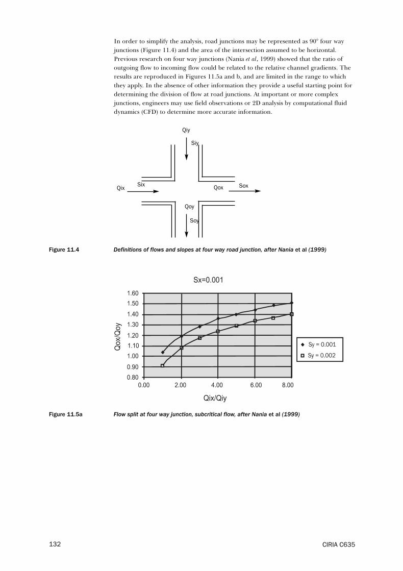
In order to simplify the analysis, road junctions may be represented as 90° four way

junctions (Figure 11.4) and the area of the intersection assumed to be horizontal.

Previous research on four way junctions (Nania et al, 1999) showed that the ratio of

outgoing flow to incoming flow could be related to the relative channel gradients. The

results are reproduced in Figures 11.5a and b, and are limited in the range to which

they apply. In the absence of other information they provide a useful starting point for

determining the division of flow at road junctions. At important or more complex

junctions, engineers may use field observations or 2D analysis by computational fluid

dynamics (CFD) to determine more accurate information.

Figure 11.4 Definitions of flows and slopes at four way road junction, after Nania et al (1999)

Figure 11.5a Flow split at four way junction, subcritical flow, after Nania et al (1999)

CIRIA C635132

Qiy

Qox

Qoy

Qix

Siy

Soy

SoxSix

Figure 11.5b Flow split at four way junction, supercritical flow, after Nania et al (1999)

11.4.4 Inlets

Flood flow may accumulate on the surface before it is discharged to a surface flood

channel. This will occur, for example, where flow is discharged from a manhole onto a

paved surface area that is near horizontal and surrounded by higher ground. There is

a risk in such cases that the level of the flood water will rise above thresholds of

adjacent property and cause flooding, or the depths created will present a risk to

pedestrians and vehicles using the area (see Section 11.4.3). The depth of water that

will accumulate depends on the relative level of the invert of entry to the flood

channel(s) and the flow discharged to the channel.

The water level required to discharge the excess flood flow into the flood channel is

dependent on whether the flood channel is mild or steep. For a mild sloping channel,

the water surface will be determined by the depth of flow in the flood channel.

1.5V2/2g (V= velocity of flow in flood channel) should be added to this to allow for

changes in energy level as the flow enters the channel. This figure includes 0.5V2/2g of

energy loss as the flow passes to the flood channel. This is illustrated in Figure 11.6a.

For a steep sloping flood channel, the depth at entry to the channel will be the brink or

critical depth as defined by Equation 11.1. The water level will be 1.5dc above the

invert (see Figure 11.6b). This analysis assumes that there is no energy loss as the flow

passes into the flood channel.

Figure 11.6a Depth of ponding governed by discharge to a mild sloping flood channel

CIRIA C635 133

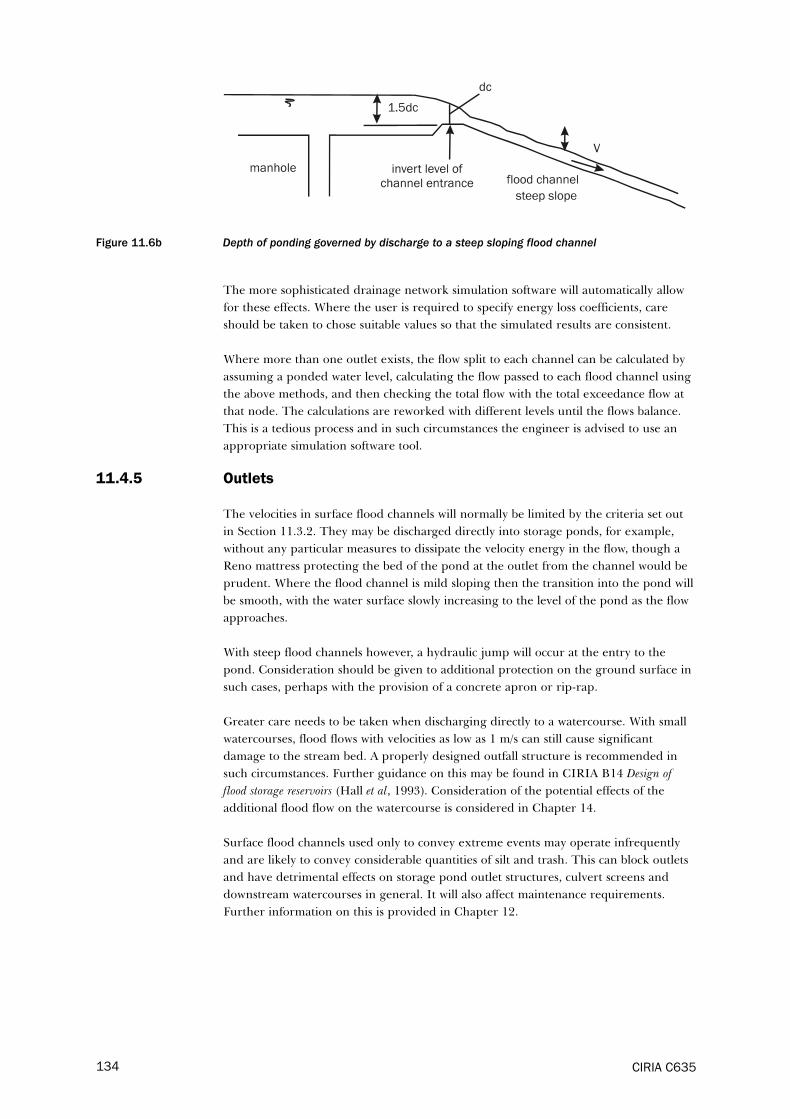
Figure 11.6b Depth of ponding governed by discharge to a steep sloping flood channel

The more sophisticated drainage network simulation software will automatically allow

for these effects. Where the user is required to specify energy loss coefficients, care

should be taken to chose suitable values so that the simulated results are consistent.

Where more than one outlet exists, the flow split to each channel can be calculated by

assuming a ponded water level, calculating the flow passed to each flood channel using

the above methods, and then checking the total flow with the total exceedance flow at

that node. The calculations are reworked with different levels until the flows balance.

This is a tedious process and in such circumstances the engineer is advised to use an

appropriate simulation software tool.

11.4.5 Outlets

The velocities in surface flood channels will normally be limited by the criteria set out

in Section 11.3.2. They may be discharged directly into storage ponds, for example,

without any particular measures to dissipate the velocity energy in the flow, though a

Reno mattress protecting the bed of the pond at the outlet from the channel would be

prudent. Where the flood channel is mild sloping then the transition into the pond will

be smooth, with the water surface slowly increasing to the level of the pond as the flow

approaches.

With steep flood channels however, a hydraulic jump will occur at the entry to the

pond. Consideration should be given to additional protection on the ground surface in

such cases, perhaps with the provision of a concrete apron or rip-rap.

Greater care needs to be taken when discharging directly to a watercourse. With small

watercourses, flood flows with velocities as low as 1 m/s can still cause significant

damage to the stream bed. A properly designed outfall structure is recommended in

such circumstances. Further guidance on this may be found in CIRIA B14 Design of

flood storage reservoirs (Hall et al, 1993). Consideration of the potential effects of the

additional flood flow on the watercourse is considered in Chapter 14.

Surface flood channels used only to convey extreme events may operate infrequently

and are likely to convey considerable quantities of silt and trash. This can block outlets

and have detrimental effects on storage pond outlet structures, culvert screens and

downstream watercourses in general. It will also affect maintenance requirements.

Further information on this is provided in Chapter 12.

134 CIRIA C635

12 Designing for surface storage

12.1 Principles of design

During extreme events, excess flow (exceedance flow) will be conveyed on the surface.

In a managed major drainage system, as advocated by this guide, this flow will be

conveyed in surface flood channels specifically designed for that purpose. However, it

may be necessary to store some of the flow above ground for two reasons: because the

capacity of designed flood channels is limited by economic constraints, or there is a

requirement to protect and not overload the downstream receptor system (see Figure

12.1 and Chapter 14):

� it will always be above ground

� it will be utilised infrequently

� the area set aside for storage may normally have a different use (primary use) eg a

playing area

� the primary use may not be available during storage operation.

Examples of areas that may be set aside for exceedance flood storage as a secondary use

are car parks, parkland and minor highways. Further information on this is given in

section 12.4. Figure 12.2 shows the inputs, processes and outputs involved in designing

the surface flood pathways for surface storage. The recommendations in this chapter

refer to both new development and retrofit applications in existing developments.

Figure 12.1 Concept of how exceedance flows are managed

12.2 Storage area design process

12.2.1 Size

The design of surface storage areas is primarily controlled by the size required and

where storage can be utilised. The flowchart in Figure 12.3 sets out the design

procedure. Due to the complexity of knowing the volume and flow conveyed away

from the area, it is likely that in all but the simplest of cases a hydraulic computer

simulation model will be used to determine the volume required. This will be used to

CIRIA C635 135

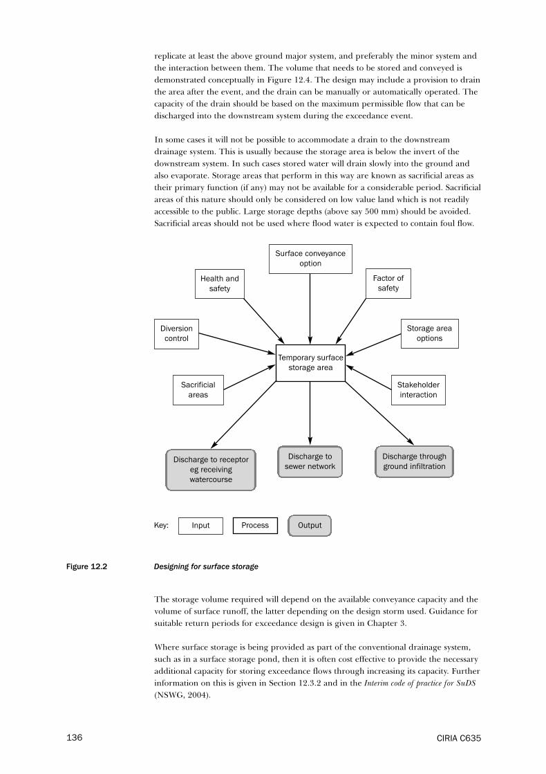
replicate at least the above ground major system, and preferably the minor system and

the interaction between them. The volume that needs to be stored and conveyed is

demonstrated conceptually in Figure 12.4. The design may include a provision to drain

the area after the event, and the drain can be manually or automatically operated. The

capacity of the drain should be based on the maximum permissible flow that can be

discharged into the downstream system during the exceedance event.

In some cases it will not be possible to accommodate a drain to the downstream

drainage system. This is usually because the storage area is below the invert of the

downstream system. In such cases stored water will drain slowly into the ground and

also evaporate. Storage areas that perform in this way are known as sacrificial areas as

their primary function (if any) may not be available for a considerable period. Sacrificial

areas of this nature should only be considered on low value land which is not readily

accessible to the public. Large storage depths (above say 500 mm) should be avoided.

Sacrificial areas should not be used where flood water is expected to contain foul flow.

Figure 12.2 Designing for surface storage

The storage volume required will depend on the available conveyance capacity and the

volume of surface runoff, the latter depending on the design storm used. Guidance for

suitable return periods for exceedance design is given in Chapter 3.

Where surface storage is being provided as part of the conventional drainage system,

such as in a surface storage pond, then it is often cost effective to provide the necessary

additional capacity for storing exceedance flows through increasing its capacity. Further

information on this is given in Section 12.3.2 and in the Interim code of practice for SuDS

(NSWG, 2004).

Discharge to receptor

eg receiving

watercourse

CIRIA C635136

Factor of

safety

Storage area

options

Stakeholder

interaction

Sacrificial

areas

Diversion

control

Health and

safety

Surface conveyance

option

Temporary surface

storage area


Discharge to

sewer network

Discharge through

ground infiltration

Storage volumes should be calculated for various duration events to determine the

critical duration for the design, ie the duration generating the maximum storage

volume requirement.

Design return periods for when storage options may be utilised are identified in

Section 12.3.1. The upper limit advocated by this guidance is the one in 200 year

return period event. However it may not be possible for a single storage area to have

this capacity. In this case the required storage volume should be distributed over more

than one area.

In general the design of surface storage areas should be in accordance with relevant

local and national practice/guidance and regulations in particular the Reservoirs Act

1975 (where applicable). Further useful guidance can be found in CIRIA B14 Design of

flood storage reservoirs (Hall et al, 1996). Each individual solution type will have some

common aspects and these are indicated in Figure 12.3.

CIRIA C635 137

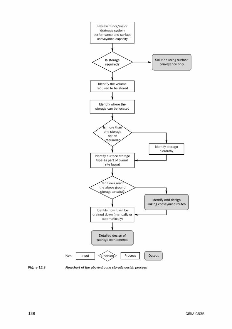
Solution using surface

conveyance only

Detailed design of

storage components

CIRIA C635138

Figure 12.3 Flowchart of the above-ground storage design process

Review minor/major

drainage system

performance and surface

conveyance capacity

Identify the volume

required to be stored

Identify where the

storage can be located

Identify surface storage

type as part of overall

site layout

Identify how it will be

drained down (manually or

automatically)

Identify storage

hierarchy

Is storage

required?

Can flows reach

the above ground

storage area(s)?

Decision

Is more than

one storage

option

required?

Identify and design

linking conveyance routes


Figure 12.4 Conceptual demonstration of the exceedance rainfall event hydrograph

12.2.2 Health and safety

Above-ground storage structures should be designed to minimise risk especially to the

general public. This will apply to those constructing, operating and maintaining the

structure as well as the public who may use the area. Careful design can eliminate or

reduce such risk. Particular attention should be given to areas such as playgrounds that

may be used by children. Table 12.1 summarises the potential hazards and gives

guidance on best practice for managing risk.

CIRIA C635 139

Table 12.1 Key health and safety areas that should be considered in the design of exceedance storageareas

Further guidance on the design of storage may be found in CIRIA’s Sustainable urban

drainage systems design manuals (Martin et al, 2000a, b, 2001), C609 Sustainable drainage

systems. Hydraulic, structural and water quality advice (Wilson et al, 2004) and B14 Design of

flood storage reservoirs (Hall et al, 1996).

12.2.3 Maintenance

Regular maintenance of surface storage areas should be undertaken as part of the

primary drainage function. The maintenance regime should reflect the secondary

(storage) function requirements. However best practice storage design should minimise

maintenance requirements. As with any form of emergency facility, maintenance will be

limited to regular inspection on operability (eg to ensure inlets and outlets are not

obstructed), and post operation inspection, clean up and remedial works. A summary of

key maintenance items is linked in Table 12.2. Further guidance on the maintenance of

storage areas may be found in CIRIA publications on SuDS and B14 Design of flood

storage reservoirs (Hall et al, 1996). This applies to the maintenance of the whole area

including the outfall and any control structures.

CIRIA C635140

Hazard Description

Access/egress This should be through designated points and where practical are separate from

where water enters or leaves the area. Where applicable sloping banks may be

used with a maximum of one in four slope, with specific areas for escape, and

access for maintenance vehicles at 1 in 12 such as in playing fields. Land should

be graded so as not to leave islands where people can be stranded.

Water depth Water depth will depend upon the area selected to retain water (see Table 12.3).

It is important to set a maximum depth and where applicable have a specific

overflow point that is utilised once the storage is full. This may only be applicable

for areas that are designed to operate between fixed return periods (eg >1 in 30

to 1 in 75). Marker posts could be positioned in the areas to indicate the depth of

the water.

Water velocity

(entering/

draining)

Flow velocity may be high, particularly at those points where flows enter into or

are drained from the area. These areas should be partitioned off if the velocities

are found to be high. High velocities may also contribute to scouring of areas.

Although its operation will be infrequent, the area should be checked after it has

operated to determine if any remedial works are required. Where possible all

velocities should be designed to be within those stated in Chapter 11.

Tripping hazards Small tripping hazards that become submerged and unseen when flows are

stored should be avoided, for example drop kerbs in a car park. Ground should be

even under foot wherever possible, with only gradual changes in level. Objects

that project above the maximum water depth will remain visible and will not

become a hazard.

Change from

primary use

Signs indicating that areas have a dual purpose should be clearly displayed to

highlight that areas may flood in very heavy rainfall. Designated access and

egress points from the area should be clearly signed in case of an emergency. Any

overland flow paths feeding into the areas should also be signed.

Sediment and

trash

After an event where storage has been utilised, a clean up operation should be

undertaken. Significant sediments may have been deposited in an area and these

will need to be removed. Repairs to the areas may be required if high velocities or

moving debris within the flow has caused damage. Areas that have contained foul

sewage may need to be treated to reduce the risk to public health.

Inlet/outlet

structures

Ideally, risks associated with inlet/outlet structures should be designed out.

Where an outlet forms part of the bank, it should slope with the bank. If penstock

controls are used, these should be located within inspection chambers.

Table 12.2 Key maintenance considerations required in the design of exceedance storage areas

12.2.4 Outfall design

The practical means of draining exceedance storage areas are:

� direct gravity connection to the sewerage system

� automatic gravity connection to receiving water

� manually operated gravity connection to receiving water

� emptying water by pump or pumped emptying

� infiltration to groundwater

� evaporation (sacrificial areas only).

The simplest method of draining surface storage areas is automatically and by gravity.

Outflow may be connected directly to the downstream sewer system or receiving water,

but in either case the impact on these systems should be assessed, as described in

Chapter 14. This is likely to be the preferred method when considering car parks,

minor roads, recreational areas, industrial areas and SuDS. Draining of a storage area

may also be achieved through infiltration, however the drain down time using this

method is likely to be large. Where there is a high risk of combined sewage flooding

occurring, draining to a combined or foul sewerage system is preferable to draining to

a watercourse.

A manually operated gravity connection to a receiving water may be used for draining

parkland and playing fields. A manual penstock housed within an inspection chamber

is likely to offer the best control while being protected from vandalism. An operating

protocol should be agreed with the body responsible for operating the receptor system.

Pumping of stored water may occur if the likelihood of the area being used is remote

CIRIA C635 141

Requirement Description

Drain downDue to the infrequent nature of operation, a manual drain down of areas may be

required, eg through pumping. If this is necessary an agreement as to when and

who will carry out the work is necessary and should be determined prior to the

designation of such areas. This responsibility is likely to rest either with the

sewerage undertaker, local authority or the environmental regulator. Areas that

naturally drain down will need to be checked to determine if this has been

achieved. The rate of drain down should be checked to minimise the risk of

stagnation or septicity of the water.

General inspection Although some areas such as playing fields and parkland may be routinely

inspected, further inspection may be required after such areas have been

used for storage. This should include checking for damage to the structure

likely to be caused by high velocities or floating debris in particular to

dedicated access/egress points, inlet/outlet controls and sloping banks.

General inspections should also take into account impacts that may arise

during its primary use.

Inlet/outlet controls Inlets and outlets should be checked on a regular basis as part of the general

maintenance of an area and also after an event has occurred where storage

has been utilised. Any blockages or debris positioned in and around the

controls should be removed. Velocity of flow entering or leaving the area

should not exceed the values suggested in Section 11.3.2.

Cleaning Significant sediment deposition is likely in areas used for storage after an

event, so a post clean up operation may be required. The removal of litter,

vegetation, sewerage debris and larger objects may be necessary Where areas

have been used to contain combined sewage, they will need to be washed

down and disinfected after use.

and no direct route to a receiving water or sewer is possible. If combined sewage is

stored and flow cannot be returned to a combined or foul sewerage system, it should be

pumped or tankered directly to a treatment works.

The draining down of such an area should be carefully considered. The receiving

system should have the capacity to receive the flows, and drain down should be

achieved ideally within a 48 hour period (eg 5.8 l/s over a 48 hour period will pass

1000 m³). Further guidance on this is given in Chapter 14.

In designing the outfall control, the receiving sewer or water should be studied to

check that reverse flow into the structure is not possible. If the outfall control is

permanently closed during operation, and only opens to drain down, then this is

unlikely to be problematic. Further advice to design outfalls is available in CIRIA C609

Sustainable drainage systems. Hydraulic, structural and water quality advice (Wilson et al,

2004) and B14 Design of flood storage reservoirs (Hall et al, 1996).

12.2.5 Diversion control design

Although storage areas will be designed to accommodate extreme events, it is possible

that the designed area is itself exceeded. This is likely to occur if a hierarchical storage

approach is taken where specific areas are designed to operate before others (identified

in Table 12.3). In this case some areas will fill to capacity and then spill through a

diversion control to other conveyance pathways and storage areas downstream,

illustrated in Figure 12.5. The design of such diversion controls should remain as

simple as possible and be compatible with the general design of the structure.

When designing a hierarchical system of storage structures, care should be taken that

the network of major system conveyance and storage adequately handles flow up to the

design return period.

Uncertainties involved in estimating exceedance flows and designing storage facilities,

means that an adequate allowance for freeboard should be incorporated into all storage

and diversion structures. For exceedance events a value of 100 mm is recommended.

Figure 12.5 Conceptual process of diverting excess flow

CIRIA C635142

12.3 Types of storage areas

12.3.1 Storage options hierarchy

Although a number of options exist for storage of above ground flows, certain areas

should be utilised before others. Table 12.3 summarises the different type of storage

facility and gives guidance on acceptable frequency of flooding. This allows the

designer to identify a hierarchy of operation where more than one type of area is

available. When selecting a storage area type, consideration should be given to the

length of time that the area may not be available for its primary function. This period

may be longer than the storm duration due to drain down and clean up operations.

More detailed descriptions of each type appear in subsequent sections.

Table 12.3 Summary of different storage options available

CIRIA C635 143

Storage area type

(primary use)Description

Maximum water

depth

Acceptable flooding

hierarchy

SuDS – detention/

retention ponds,

infiltration basins

etc

Additional storage used to attenuate

peak flows for all storms up to normal

design events. Volume of such

structures could be increased to retain

exceedance event volumes depending

upon available area.

Varies

depending

upon storage

area design

> 1 in 30 y SW

> 1 in 100 y CS

Car parks Used to temporarily store exceedance

flows. Depth restricted due to potential

hazard to vehicles, pedestrians and

adjacent property. Could be residential,

commercial or industrial.

0.2 m > 1 in 30 y SW

> 1 in 30 y CS

Recreational areas Hard surfaces used such as basketball

pitches, five-a-side football pitches,

hockey pitches, tennis courts.

0.5 m unless

area can be

secured, then

1.0 m

> 1 in 30 y SW

only

Minor roads Minor roads typically where maximum

speed limits are 30 mph. Depth of water

can be controlled by design.

0.1 m > 1 in 30 y SW

> 1 in 30 y CS

Playing fields Used for sport such as football and

rugby. Set below the ground level in the

surrounding area and may cover a wide

area and hence offer large storage

volume.

0.5 m unless

area can be

secured, then

1.0 m

> 1 in 20 y SW

only

Parkland Has a wide amenity use. Often may

contain a watercourse. Care needed to

keep water separate and released in a

controlled fashion to prevent sudden

downstream flooding.

0.5 m unless

area can be

secured, then

1.0 m

> 1 in 30 y SW

> 1 in 100 y CS

School

playgrounds

Hard standing area of schools could

provide significant storage. Extra care

should be taken when designing such

areas due to high number of children.

0.3 m > 1 in 30 y SW

only

Industrial areas Low value storage areas. Care should be

taken in the selection as some areas

used could create significant surface

water pollution.

0.5 m > 1 in 50 y SW

> 1 in 100 y CS

Major roads/

motorways

Due to their primary function and

importance only used for severe events.

0.1 m > 1 in 100 y SW

> 1 in 100 y CS

Key: SW = surface water flooding CS = combined sewerage system flooding y = year

12.3.2 Additional storage in SuDS

When considering the type of areas used to store exceedance events, SuDS

arrangements should not be overlooked as these can be very effective in attenuating

exceedance flows (Evans et al, 2004). The use of such systems to retain and attenuate

exceedance flows is becoming more common. Maintenance, ownership of and the legal

framework issues surrounding the design and use of such systems is now being resolved

using model agreements (Shaffer et al, 2004, and NSWG, 2004).

Much work has already been completed and published to aid practitioners in designing

such systems. In terms of above ground storage though, basins and ponds are the most

appropriate types. More technical guidance is given in CIRIA C522 Sustainable urban

drainage systems – design manual for England and Wales (Martin et al 2000a) and C609

Sustainable drainage systems. Hydraulic, structural and water quality advice (Wilson et al,

2004).

The design of ponds, detention basins and infiltration basins can be undertaken using

the current guidance listed above. SuDS are normally designed to work and

accommodate runoff generated from more frequent occurring storms. This needs to be

taken into account if such areas are to be upgraded to accommodate additional storage

during extreme events.

The calculation of the extra volume available will enable the design of these systems to

be more appropriately sized. The likely changes are to be to the plan area, depth and

levels of surrounding site. The normal size of a pond or basin may only need a small

increase in depth around the perimeter of the normal operating design to provide

significant extra storage. This increase in size should be located in the safety bench or in

the main area (Figure 12.6). The design of ponds and basins may require an extreme

event overflow. This may need to be redesigned if the system is to accommodate

exceedance flow. There may still be the need for a diversion control if the volume

exceeds the additional amount provided (eg in a hierarchy of surface storage systems).

Figure 12.6 Cross-section through an infiltration or detention pond designed to accommodateexceedance

12.3.3 Car parks

Car parks may become storage areas for exceedance flows by default during an

extreme event. Surface ponding can regularly be seen on car parks that are poorly

finished due to uneven surfaces. Discharge from a car park into the minor system can

be limited and this can also contribute to surface ponding (Figure 12.7). The volume

stored will depend on the perimeter design and in particular the kerb height at the

lowest point. Traditionally, the kerb height is designed to be 100 mm to avoid damage

to vehicles that overhang the kerb.

CIRIA C635144

Figure 12.7 Temporary ponding in car park showing the storage potential during an extreme event

It is possible to increase the storage volume by raising kerbs at specific locations on the

perimeter or by grading the surface to increase the kerb level relative to the low point

of the car park. A long profile berm (Walesh, 1999) can also be positioned across the

entrance to control the stored water. Berms are considered to be similar to speed

humps (although their aim is to not act as a speed control), however they may be

longer to avoid the discomfort experienced with speed humps. These long profile

berms have been successfully used in Chicago in the United States (Walesh, 1999) to

temporarily store water during normal and exceedance rainfall events. Health and

safety fears such as freezing or standing water has proved not to be a problem to date

(Walesh, 1999). An example of a long profile berm is shown in Figure 12.8.

Figure 12.8 Example berm profile (adapted from Walesh et al, 1999)

Due to the nature of car parks it is unlikely that there will be any significant flow

velocity, however it is recommended that the depth of storage be limited to 0.2 m (see

Chapter 11). This is lower than other figures in use elsewhere with 0.3 m being a

typical value (Regional Flood Control District, 1999). However by restricting the depth

of water to 0.2 m, damage to motor vehicles should be minimal.

Any surrounding buildings should be set with thresholds above top water level. This

offers protection if the water level overtops the kerb level if a flood wave from a moving

vehicle is produced. The depth of flood wave is primarily dependent upon the depth of

flow and velocity of the vehicle. An initial flood wave created by a moving vehicle

reduces and dissipates as the distance increases. So if parking bays are located either side

of the access road, any flood damage will be minimal (Figure 12.9). If building

thresholds are close to where a flood wave might be generated, the freeboard should be

increased accordingly, or vehicle movements restricted during extreme events.

CIRIA C635 145

The greatest potential for utilising such storage will be on business and industrial

parks, and commercial shopping locations. There may also be potential with communal

parking bays in residential areas. The design should take into account the likely use of

such a facility. Large car parks offer significant storage volume potential, and a staged

or zoned approach could be taken. Areas furthest away from the premises should be

designed to flood first with different areas segregated by berms.

Consideration should be given to keeping disabled bays above the top water level.

12.3.4 Minor roads

The use of minor roads for the secondary function of storm conveyance is now open to

consultation (Defra, 2004). The use of minor roads for this function in other countries

has taken place for a number of years (Walesh, 1999, Regional Flood Control District,

1999, and Nania et al, 2002). Minor roads have also been used to store exceedance

volume. A recent study in Bangkok indicated that the cost of implementing storage to

receive all runoff could be substantially reduced if street storage was employed

(Boonya-aroonnet et al, 2002).

Utilising storage within the minor road network requires careful design. Consideration

should be given to the position of storage locations. If a large number of such locations

are selected, the potential storage volume is large. The use of long profile berms in the

minor road network, where vehicles should be travelling slowly, may enable additional

storage to be provided. An example of a long profile berm to enable storage is shown

in Figure 12.10.

CIRIA C635146

Figure 12.9 Conceptual arrangements to temporarily store exceedance runoff in a car park

The positioning of the storage and any long profile berms should be agreed during the

layout and design stage and when a known storage volume has been identified.

Highway storage should be restricted to residential/business park locations where the

speed limit is 30 mph or less, and their position effectively signed. Typical signage used

around the world indicates that the road is liable to flooding during heavy rainfall

periods and caution should be taken when driving through the area (ie reduce speed).

Provided that berms have sufficiently long profile they can made compatible with

horizontal alignment designed to control speed. The creation of ponded areas by

artificially raising the kerb height is not recommended as this may mislead the motorist

or pedestrian as to the depth of water on the highway. Surface storage may be filled

and drained from the low points using conventional gullies, though kerb inlet gullies

may be more suitable for this purpose.

Figure 12.10 Example of the storage that can be achieved and examples of berms (courtesy Walesh)

CIRIA C635 147

12.3.5 Playing fields, recreational areas and parkland

The use of recreational areas such as playing fields to control and temporarily store

surface water flows has been acceptable practice for a number of years (Wisner and

Kassem 1982; Hall et al, 1996).

By design, the frequency of flooding in such areas will be low. However during an

extreme event, significant quantities of water may be stored. The design of conveyance

pathways to such areas should be carefully considered to ensure that flows can reach

them and not cause flooding elsewhere in the catchment. It is crucial that any

parkland, recreational area or playing field used for storage is considered during the

early stages of the development process. An example of this is shown in Figure 12.11.

Sign posting of such areas is very important and should state that the area is a dual

drainage-recreational area and as such could be subject to flooding during wet weather

conditions. Recreational areas could include outdoor five-a-side football or basketball

pitches that are lower than the ground level and could provide additional storage

relatively cheaply.

As these areas are often larger than other flood storage areas, careful consideration

should be given to filling and emptying. Public using such areas should have an

obvious and direct means of escape when such areas fill. Escape pathways should be

kept separate from flood pathways. Velocities during filling and emptying may be

significant and the areas should have relatively flat or gently sloping bases. Ground

levels should be graded to avoid islands during filling that may leave people stranded.

Figure 12.11 A dual-purpose recreational baseball pitch/storage area in Japan. This is significantly lowerthan the surrounding ground level (courtesy Shoichi Fujita)

CIRIA C635148

13 Building layout and detail

13.1 Design principles

There are numerous pressures applied to property developers and many different

design considerations required during the design process. This chapter focuses on

issues that relate to property flooding and how small changes in layout and design may

improve the level of protection from flooding.

When deciding on the drainage of a new development, the designer should identify

and consider the use of natural flood pathways in the undeveloped area. As a general

principle, the closer artificial drainage and above ground flood pathways follow the

natural layout, the more effective the drainage system will be.

Planning Policy Guidance Note 3 Housing (PPG3) places pressure on housing developers

to increase the building density to between 30 and 50 dwellings per hectare. This is

against a traditional number of 23 dwellings per hectare for suburban estates (Shaffer et

al, 2004a and b). Increased pressure could lead to a reduction in available space for some

SuDS components and above ground storage areas. The guidance provided in PPS25

(CLG, 2001) where it encourages the incorporation of measures for effective flood

control, may create tension. Other publications such as Sewers for adoption 5th edition

(Water UK and WRc, 2001) highlights that above ground pathways should be considered

during design. BS EN 752-3:1996 also identifies that during the planning stage overland

flow paths may influence the site design. CIRIA C624 Development and flood risk – guidance

for the construction industry (Lancaster et al, 2004) addresses this by promoting a consistent

approach to planning in relation to flood risk.

Drainage and flood control issues should be considered at the start of the development

process when site layout is first set out. Fixing building layout prior to drainage

considerations significantly limits the potential for effective control of flood water in

extreme events. The factors that should be considered are summarised in Figure 13.1.

Careful planning and consideration of development layouts can facilitate the

management of flood risk. Development layout can significantly affect how flows will be

conveyed and may even contribute to property flooding. In particular, channels and

areas that may act as conveyance pathways and storage areas should be identified early

in the process. The flowchart in Figure 13.2 simplifies the overall design process.

13.2 Building type and layout

13.2.1 Layout and flood pathways

Identifying the route of flood pathways in a development is a key design process that

can assist with managing flood risk. Once flood pathways have been identified, the

subsequent effect on downstream receptor systems should be considered. Conveyance

pathways, storage areas and the downstream receptors all interact with the

conventional drainage system, so the design process tends to be heavily interactive, with

the final design often differing significantly from the outline proposal. Adequate time

should be allowed to complete this stage of the site development process.

CIRIA C635 149

Figure 13.1 Processes involved with designing building layout for exceedance events

An example of the route of above ground flood pathways in a development is shown in

Figure 13.3. This example also indicates how temporary above ground storage has

been incorporated into the design. Consideration should be given at initial layout

design stage of any site features that might be incorporated, such as playing areas,

fields, detention ponds, infiltration basins, car parks and minor roads. Normally the use

of dual-purpose areas will be the most cost effective and the greatest benefit to the

community.

CIRIA C635150

Exceedance

storage position

Minimise runoff

Property elevation

Venting details

Selection of

construction materialsBuilding and road

layout, initial and

outline designEntrance and

driveway details

Exceedance flood

risk assessment

Flood

pathways

Individual property

flood risk assessment

Final site

design

Surface storage

locations planned

Building position

Existing topography

Site

elevations

Stakeholder

interaction

Conveyance

routes planned

and recorded


Figure 13.2 Flowchart showing the process of including building detail and layout in the design processwhen considering the exceedance flood pathways

Complete major/ minor

system design

CIRIA C635 151

Obtain topographic

data and inspect site.

Identify existing flood

pathways

Design initial

site layout

Consider building

detail to prevent or

reduce impact of

flooding

YES (1)

YES (2)

NO

Decision

Does exceedance

flood risk assessment

identify properties are at

risk of flooding?

Add more surface

conveyance channels

or storage


Figure 13.3 Example of major and minor systems in a site layoutNote: The pathways created between housing clusters to allow overland flow to drain from undeveloped areas behind

property.

13.2.2 Utilising existing features of the site

It is important to consider numerous aspects in the design from the outset to produce

an integrated solution that satisfies all stakeholders. Auckland’s Regional Council

technical publication Stormwater management devices: design guide manual (Auckland

Regional Council, 2003) identifies four techniques that can be used during the initial

design layout to minimise runoff:

� retain natural drainage site features

� good runoff control practices

� clustering of properties together

� minimise earthworks and ground disturbance.

It is important that these techniques are considered at the start of the design process.

Where possible the natural drainage site features should be retained and the position

of houses built around these. In particular, the location of watercourses and dry valleys

CIRIA C635152

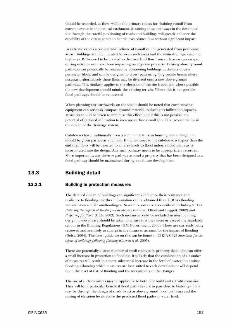
should be recorded, as these will be the primary routes for draining runoff from

extreme events in the natural catchment. Retaining these pathways in the developed

site through the careful positioning of roads and buildings will greatly enhance the

capability of the drainage site to handle exceedance flow without significant impact.

In extreme events a considerable volume of runoff can be generated from permeable

areas. Buildings are often located between such areas and the main drainage system or

highways. Paths need to be created so that overland flow from such areas can escape

during extreme events without impacting on adjacent property. Existing above ground

pathways can potentially be retained by positioning buildings in clusters or as a

perimeter block, and can be designed to cross roads using long profile berms where

necessary. Alternatively these flows may be diverted onto a new above ground

pathways. This similarly applies to the elevation of the site layout and where possible

the new development should mimic the existing terrain. Where this is not possible

flood pathways should be re-assessed.

When planning any earthworks on the site, it should be noted that earth moving

equipment can seriously compact ground material, reducing its infiltration capacity.

Measures should be taken to minimise this effect, and if this is not possible, the

potential of reduced infiltration to increase surface runoff should be accounted for in

the design of the drainage system.

Cul-de-sacs have traditionally been a common feature in housing estate design and

should be given particular attention. If the entrance to the cul-de-sac is higher than the

end then flows will be directed to an area likely to flood unless a flood pathway is

incorporated into the design. Any such pathway needs to be appropriately recorded.

More importantly, any drive or pathway around a property that has been designed as a

flood pathway should be maintained during any future development.

13.3 Building detail

13.3.1 Building in protection measures

The detailed design of buildings can significantly influence their resistance and

resilience to flooding. Further information can be obtained from CIRIA’s flooding

website: <www.ciria.com/flooding/>. Several reports are also available including SP155

Reducing the impacts of flooding – extemporary measures (Elliott and Leggett, 2002) and

Preparing for floods (CLG, 2003). Such measures could be included in most building

design, however care should be taken to ensure that they meet or exceed the standards

set out in the Building Regulations (HM Government, 2000). These are currently being

reviewed and are likely to change in the future to account for the impact of flooding

(Defra, 2004). The latest guidance on this can be found in CIRIA C623 Standards for the

repair of buildings following flooding (Garvin et al, 2005).

There are potentially a large number of small changes in property detail that can offer

a small increase in protection to flooding. It is likely that the combination of a number

of measures will result in a more substantial increase in the level of protection against

flooding. Choosing which measures are best suited to each development will depend

upon the level of risk of flooding and the acceptability of the changes.

The use of such measures may be applicable to both new build and retrofit scenarios.

They will be of particular benefit if flood pathways are to pass close to buildings. This

may be through the design of roads to act as above ground flood pathways and the

raising of elevation levels above the predicted flood pathway water level.

CIRIA C635 153

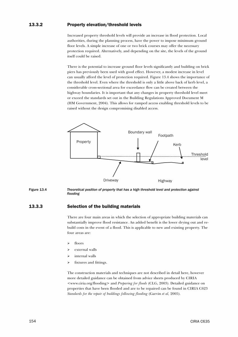
13.3.2 Property elevation/threshold levels

Increased property threshold levels will provide an increase in flood protection. Local

authorities, during the planning process, have the power to impose minimum ground

floor levels. A simple increase of one or two brick courses may offer the necessary

protection required. Alternatively, and depending on the site, the levels of the ground

itself could be raised.

There is the potential to increase ground floor levels significantly and building on brick

piers has previously been used with good effect. However, a modest increase in level

can usually afford the level of protection required. Figure 13.4 shows the importance of

the threshold level. Even where the threshold is only a little above back of kerb level, a

considerable cross-sectional area for exceedance flow can be created between the

highway boundaries. It is important that any changes in property threshold level meet

or exceed the standards set out in the Building Regulations Approved Document M

(HM Government, 2004). This allows for ramped access enabling threshold levels to be

raised without the design compromising disabled access.

Figure 13.4 Theoretical position of property that has a high threshold level and protection againstflooding

13.3.3 Selection of the building materials

There are four main areas in which the selection of appropriate building materials can

substantially improve flood resistance. An added benefit is the lower drying out and re-

build costs in the event of a flood. This is applicable to new and existing property. The

four areas are:

� floors

� external walls

� internal walls

� fixtures and fittings.

The construction materials and techniques are not described in detail here, however

more detailed guidance can be obtained from advice sheets produced by CIRIA

<www.ciria.org/flooding> and Preparing for floods (CLG, 2003). Detailed guidance on

properties that have been flooded and are to be repaired can be found in CIRIA C623

Standards for the repair of buildings following flooding (Garvin et al, 2005).

CIRIA C635154

13.3.4 Venting

Flow may enter into a property through a variety of venting systems. The most

common of these will be through an air brick and its subsequent vent channel due to its

relatively low position. In older properties air bricks may be positioned lower than

those in newer properties with the vent channel passing straight through the wall.

Newer properties may have periscope venting channels which are higher at the air

brick and lower internally (Figure 13.5). It is important when detailing buildings that

any buildings that may be subject to flooding have the air vents above the likely flood

depth. Alternatively, an automatic flood seal can be fitted to each vent.

Figure 13.5 Periscope venting detail (adapted from CIRIA, 2003a)

13.3.5 Entrance details

The elevation of the entrance to a property can act as a line of defence to prevent

flooding. This will be effective if the threshold is above the top water level of any flood.

Where possible the entrance level should be set with a 50 mm free board allowance

above the expected top water level. Where this is not possible, the risk of the curtilage

and property being flooded should be assessed. This will depend upon the property

elevation and access slope and this risk can be mitigated with the design of other

elements. Where the property threshold is below back of footpath level, the back of

footpath level should not be lowered to ease the driveway gradient, as this would

encourage exceedance flow conveyed within the highway to divert into the property.

Further information on this is given in Appendix 3.

13.3.6 Driveways and curtilage

The slope and the surrounding land within the curtilage will define whether water will

flow towards or away from a property. Where possible, gardens and drives should slope

away from the property. Where this is not possible, greater consideration should be

CIRIA C635 155

given to increasing the ground level of the property and possible entry points for flood

water.

The area in the immediate vicinity around a building should be sloping. Approved

Document H of the Building Regulations (HM Government, 2002) identifies that a

reverse gradient from the property should be created for at least 500 mm with a cross

fall recommended at one in 60. However for exceedance flows, this may need to be

increased. If a flood pathway is designed to pass close to a building the size will greatly

depend upon the calculated water depth.

Gardens at the front and rear of the property should be lower than the property itself.

Case studies show that properties with gardens at a higher level that slope and drain

towards the house can direct substantial quantities of flow towards the property which

can lead to flooding if no flood pathway away from the building is provided (Figure 4.3).

13.3.7 Siting of services

The position of services should be kept above possible flood water levels. This

particularly applies to electrical and gas appliances which needs to be inspected by a

qualified engineer following flooding before they are re-used. Any meters should also

be positioned as high as possible. Where services are located in the basement, they

should be at ceiling height to offer the maximum protection possible. Further advice on

the position of services and appliances is given in Preparing for floods (CLG, 2003),

SP155 Reducing the impacts of flooding – extemporary measures (Elliott and Leggett, 2002)

and Advice sheet 7 Flood-resilient services (CIRIA, 2003b).

13.3.8 Inadvertent modifications to existing flood pathways

Flooding by default can often occur because of the inadvertent modifications to existing

flood pathways. This may be through an extension to a property such as garages,

conservatories or even the construction of new fence or wall on the boundary that block

or re-routes a flood pathway (Figure 13.6). Property A has a driveway that enables

exceedance flows to pass and not cause flooding. Property B shows the same property

but with an extension. Exceedance flows, having no flood pathway, initially cause

surface ponding followed by property flooding. This could even occur during minor

storms. It is important that all overland flow paths are recorded and any proposed

changes to a property take into account these flow paths.

The challenge of keeping the pathway clear in the future is difficult, although a

number of measures can be set in place in an attempt to preserve such designed

pathways. Designed flood pathways should be recorded on the approved drawings of a

planning consent. This will alert planning officers to the existence of the flood

pathways when they consider a new application. Where a development is disposed of in

a number of separate lots, such as with a typical housing development, restrictive

clauses should be included in the transfer or assignment titles to protect the rights of

adjacent plots to the conveyance of flood flow.

CIRIA C635156

Figure 13.6 Plan view of how extensions to property can cause flooding by removing an existing floodpathway

13.3.9 Under building flood paths

Under building flood paths may exist by design or by default. If it is known that a flood

pathway exists, where practical, the building should be repositioned or the flood

pathway re-routed. However if neither of these options are viable, there may be the

need to incorporate the design of the flood pathway into the design of the property.

This is likely to mean that an open area is created, for example at a car park that could

be used to control the flows or alternatively provision is made to pass the flow under

the building. If the flow is to pass underneath the building, settlement and protection

of the foundations should be considered, as well as ensuring there is sufficient capacity

for the flow. Approved Document C of the Building Regulations (HM Government,

2004) addresses this issue. If the flow is to be routed above ground, the structure

should be designed to allow a free flow into, through and away from the structure.

Obstructions to the flow should be avoided.

CIRIA C635 157

14 Downstream impact assessment

Creating additional conveyance by utilising above ground flood paths could have

significant adverse effects on downstream systems, for example by transferring flooding

from one area to another. When a solution is implemented it is important to identify

the consequences downstream and undertake any mitigation measures that are

necessary.

When assessing the downstream impact the approach should be to consider the

assimilative capacity of the receiving system and the spatial extent to which the

assessment is necessary. This should then be applied to how this affects the various

stakeholders.

14.1 Conveyance and storage

The downstream implications of a proposed solution will vary depending on the

receiving system and the proposed solution itself. It is likely that conveyance solutions

will be predominantly used to transfer flows from one area that suffers from a risk of

flooding, to another. The implications of this for the receiving system may be

significant, with high flow rates and volumes being transferred over a short period of

time. Alternatively where storage forms part of the solution, the impact on the

receiving system may be less due to the attenuation effects of the storage volume.

In either case, the assimilative capacity of the receiving system should be adequately

assessed in order to determine if further storage is required to mitigate adverse effects.

14.1.1 Flood conveyance impacts

Conveyance of flood exceedance flows commonly makes use of road surfaces and other

surface pathways, depending on the topography and land use of the site. The impact

downstream may be significant if flood water is passed on to other areas which may also

be suffering from flooding. Additional flow conveyed from the upstream system may

add to an already overloaded downstream system significantly increasing flood risk in

that area. The flood extent and risk can be exacerbated when areas receive high

upstream flow and an increase in conveyed flood flow rates.

Assessment of the spatial extent of potential impact is very difficult in an urban

environment. In the situation where the flow discharges to an open channel or river

that serves an area which is at least 20 times greater than the area causing the flooding,

it is unlikely that the impact downstream will be significant. However where flow is

discharged to another urban drainage system, where streets confine flood flows and

pipe systems can convey large volumes of water to hydraulic low points elsewhere, a

more detailed assessment is necessary.

Consideration of the overland flow paths and also the sewerage system capacity is

probably necessary to determine the impact of the flood flow. Drainage simulation

modelling is likely to be needed in many instances to carry out this an accurate

assessment.

CIRIA C635158

14.1.2 Conveyance with storage

Where storage has been provided within the upstream area, in order to manage flood

risk, the downstream impacts are likely to be less than with a conveyance only solution.

This is because the storage attenuates the runoff, reducing peak flow, and spreading

the flow hydrograph over a longer time period. However there will be occasions where

storage can be detrimental to downstream systems. This will occur in cases where the

storm response time in the downstream system is significantly longer than that in the

urban system, such as occurs when a small to medium sized urban area discharges to a

river system fed from a large upstream rural catchment.

In such cases, the effect of storage can be to delay the runoff so that its peak flow

occurs around the same time as the peak response in the receiving river. Without

storage, the peak in the urban runoff will discharge before peak flow occurs in the

river. Without storage it may be possible to accommodate the additional urban flow

within the capacity of the existing river system.

14.2 Procedure for assessing and mitigating impacts

The procedure for assessing the impacts of exceedance flow and then for designing and

implementing any required mitigation measures is set out in Figure 14.1.

14.3 Assessing the impact on downstream systems

To avoid an incomplete assessment of impacts it is useful to consider all the various

stakeholders that might be affected by the impact from upstream exceedance flows.

Such stakeholders may be affected because:

� their property or land is damaged by flood flows resulting from the impact

� there is an increased risk to their personal health or safety

� there is an increase in the liability for the statutory or non-statutory function they

are required to fulfil.

CIRIA C635 159

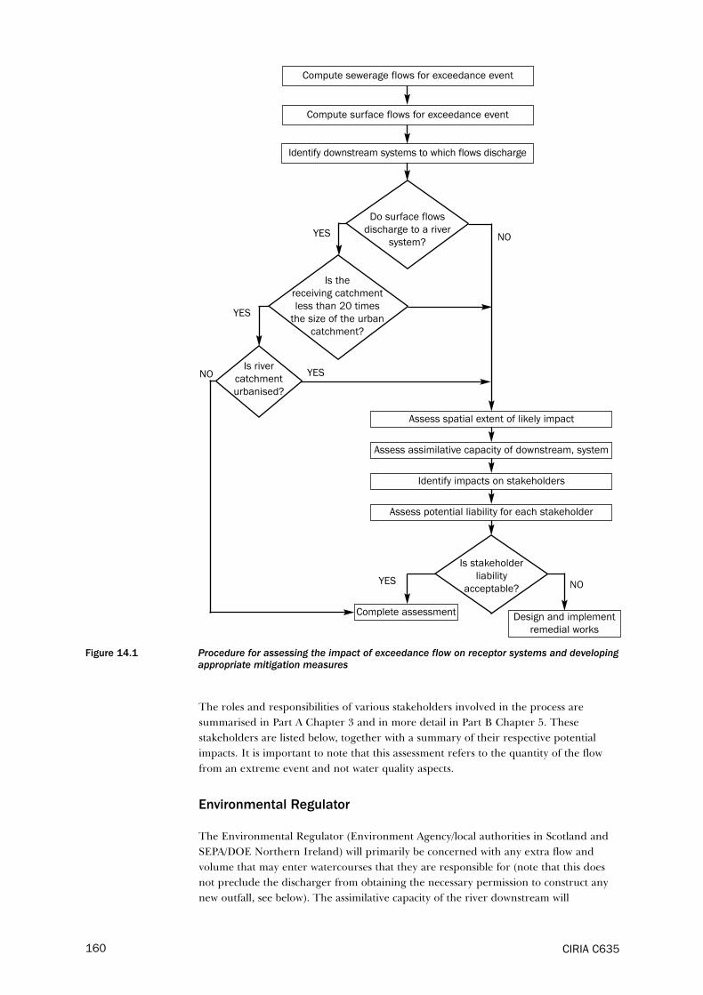
Figure 14.1 Procedure for assessing the impact of exceedance flow on receptor systems and developingappropriate mitigation measures

The roles and responsibilities of various stakeholders involved in the process are

summarised in Part A Chapter 3 and in more detail in Part B Chapter 5. These

stakeholders are listed below, together with a summary of their respective potential

impacts. It is important to note that this assessment refers to the quantity of the flow

from an extreme event and not water quality aspects.

Environmental Regulator

The Environmental Regulator (Environment Agency/local authorities in Scotland and

SEPA/DOE Northern Ireland) will primarily be concerned with any extra flow and

volume that may enter watercourses that they are responsible for (note that this does

not preclude the discharger from obtaining the necessary permission to construct any

new outfall, see below). The assimilative capacity of the river downstream will

CIRIA C635160

Compute sewerage flows for exceedance event

Compute surface flows for exceedance event

Identify impacts on stakeholders

Design and implement

remedial works

Complete assessment

Assess spatial extent of likely impact

Assess assimilative capacity of downstream, system

Assess potential liability for each stakeholder

Identify downstream systems to which flows discharge

YES

YES

YES

YES

NO

NO

NO

Do surface flows

discharge to a river

system?

Is stakeholder

liability

acceptable?

Is the

receiving catchment

less than 20 times

the size of the urban

catchment?

Is river

catchment

urbanised?

determine whether or not the discharge will have a significant impact. In assessing the

impact, account should be taken not only of the peak rate of discharge, and volume

discharged, but also the timing of the event. As explained previously, where the timing

of the peak of the discharge differs significantly from the peak in the river, it may be

possible to accommodate the additional discharge without significant impact.

Potential impacts may stretch for a considerable distance downstream and in some cases

upstream. The EA will advise on the spatial extent of any required assessment.

A second concern may be the quality of the water entering the watercourse. Although

water quality is not considered as part of the guidance, it should be noted that if the

new discharge to the watercourse occurred frequently this might become an issue.

Environmental regulators are responsible for flood control and flood mitigation for

watercourses within their control, but are not liable for consequential damage.

Land drainage authorities (including this function in local authorities)

Land drainage authorities will have similar concerns to the Environmental Regulator

for any additional flow being discharged to a watercourse that is their responsibility.

Any increase in flow into these watercourses may cause flooding further downstream,

so identifying the spatial extent is very critical.

There are no simple rules for determining the spatial extent in such cases, as this

depends on local conditions. In the first instance the route for draining exceedance

flows through the receptor system should be traced out on a suitable plan. Limitations

to the drainage capacity of the various downstream sections should be identified. In

particular the capacity of culverts, bridge openings and key conveyance channels

should be assessed. The critical sections should be marked on a plan and potential

areas of flooding identified by inspection of existing ground levels. This will identify

the extent of the area that may require more additional assessment for flood impact.

Riparian owners and other owners of receiving waters

The consent of the relevant riparian owner is required where a new outfall is to be

constructed. In granting consent, the owner will assess the likely impact and may

require additional works to mitigate against perceived impacts.

Highway authorities

Highway authorities (Highways Agency/local authorities) are responsible for highway

drainage, highway maintenance and the safety of highway users. They will have a

particular concern that any additional surface flow that discharges onto a highway

surface may have an impact not only on highway drainage capacity, but also on the

structural condition of the highway and/or the safety performance. The former is

unlikely to be significant if the occurrence of the extreme event is rare (which will

normally be the case). The latter is likely to be more important as highway authorities

are becoming increasingly exposed to litigation following accidents where the cause has

at least in part been attributable to standing water. Adhering to the limitations of velocity

and depth recommended in Chapter 11, should mitigate these effects. At the very least

an agreement to discharge onto a highway surface would normally be required between

the highway authority and the stakeholder proposing to discharge the flow.

CIRIA C635 161

Sewerage undertakers

The conveyance of surface flows into a downstream sewerage system may cause hydraulic

overloading and subsequent flooding for which the sewerage undertaker is liable. As

explained in Chapter 5, a sewerage undertaker only has a responsibility to effectually

drain property, and will argue that it is not their responsibility to drain other areas, nor to

handle extreme events. Where the additional surface flow is shown to reduce the existing

level of service of a sewerage system, normally determined by computer simulation, the

undertaker may require mitigation measures to restore the original level of service.

Insurance industry

The insurance industry will be interested in the transfer of flood risk from one area to

another as a result of the implementation of a solution. This will be critical when a

property owner’s liability changes and their own liability is affected. Insurers will

normally try to offset any perceived increase in risk through an appropriate increase in

insurance premiums, imposed excess and/or limitations to benefit.

Land owners

Where surface water is discharged onto private property in such a way as to

deliberately cause flooding (as would be the case in discharge from a surface flood

channel), a right to flood agreement would be necessary between the landowner and

the stakeholder wishing to discharge. In reaching such an agreement, the following

should be taken into consideration.

1. Who has the right to flood at the moment?

2. What compensation is payable in exercising the right to flood?

3. Whose land is affected?

4. How would the land used for flood conveyance and storage be protected?

5. How will the property owners insurance be affected?

Consideration would also have to be given to the future maintenance of such areas and

any necessary clean-up following an extreme event. Further details of this are given in

Chapter 12.

Care should be taken to fully evaluate the health and safety risks to the public caused

by any agreement to flood. The relatively short times of concentration in urban areas

means that it may not be possible to give adequate flood warnings, so it will not be

possible to actively manage such flooding. Consideration should be given to

appropriate signage and the education of local community groups.

14.4 Mitigating the effects of downstream impacts

Mitigation measures will be needed where there is insufficient assimilative capacity in

the receptor system. Mitigation can be achieved by providing a storage facility close to

the point of discharge. If this is not possible, additional storage may be distributed in

the area upstream.

The amount of storage volume required will depend on how the flow is to be limited.

As mentioned previously, the analysis should extend not only to look at the effects on

peak flow and volume, but also to compare the timing of the peak flow in the upstream

system with the peak flow in the receptor.

CIRIA C635162

Receptor systems may often be hydraulically overloaded at the time of peak discharge,

because they also are suffering from the effects of the same extreme event. However,

there may be other causes of overloading in the receptor system. The effects of a

sudden extreme event in summer, when river levels are low, may be different from

winter when levels are higher. Where discharges are to coastal areas, impacts may be

affected by tide levels. Some form of joint probability analysis may be required.

Addressing the needs of flood exceedance is unlikely to result in standard drainage

solutions for extreme events. Storage is much more likely to be provided by mobilising

flooding of certain roads, car parks, playing fields and other temporary flood areas

where the consequences and capital costs are limited.

Consideration should be given to creating sacrificial areas in areas of low land value,

where flood water from rare extreme events can be stored over long periods. Water

from such areas could then infiltrate slowly into the ground and/or evaporate. Care

should be taken to fully address the health and safety aspects of such measures, as

explained in Chapter 12.

CIRIA C635 163

CIRIA C635164

Part C Case studies

15 Case study 1: Bishopbriggs South

15.1 Introduction

The Bishopbriggs South catchment lies to the north of Glasgow. The catchment covers

an area of some 350 hectares and has a population of 18 000. In 2002 the area suffered

from an extreme rainfall event of between 30 and 100 year return period. This caused

extensive flooding of property. Subsequent analysis showed that in addition to the

effects of runoff from the developed areas, the sewerage system also suffered from

additional flow from permeable areas adjacent to the developed area, and from backing

up of outfalls from local watercourses that were themselves overloaded.

The catchment is largely made up of medium density housing in the form of semi-

detached and terraced property. The minor drainage system consists primarily of

combined sewers, though part of the area is separately drained. Trunk sewers mostly

run parallel to the Bishopbriggs Burn, which is the principal watercourse. The minor

system drains to the Kelvin Valley trunk sewer, the minor drainage system is shown in

Figure 15.1.

Little is known of the history development of the catchment. The majority of the

development is post-war and it is likely that the sewerage system is contemporary with

this. The system is thought to be structurally sound and infiltration minimal.

15.2 Stakeholder involvement

The flooding of 2002 which affected a large number of properties caused a public

outcry. There was considerable press coverage with adverse commentary largely being

aimed at Scottish Water and East Dunbartonshire Council, the local unitary authority.

In the weeks following, these two bodies agreed to collaborate to find suitable solutions

to managing flood risk in the area.

Scottish Water are responsible for draining developed areas provides an agreed level of

protection against flooding, which in this area is the 30 year return period rainfall

event. Flow from highway drains are the responsibility of East Dunbartonshire Council

and the Council is also responsible for land drainage and the maintenance of local

watercourses. Scottish Water agreed to address their responsibilities with respect to the

performance of the sewerage system while East Dunbartonshire Council agreed to

address any deficiencies in draining permeable areas and ensure adequate capacity in

local watercourses, especially the culverted sections.

The following sections illustrate how the recommendations in this guidance can be

applied to the Bishopbriggs catchment to understand the performance of its drainage

systems in extreme events and to assess proposed remedial measures.

CIRIA C635166

Figure 15.1 Bishopbriggs South sewerage system

15.3 Calculating exceedance flow

The process for calculating exceedance flow is set out in Chapter 9. The network is not

particularly large, but is complex because of the interactions with local watercourses

and the input of overland flow from permeable areas. A level 2 study (Box 9.1) is

selected initially. Figure 9.2 summarises the various inputs to the process and Figure

9.5 sets out the different steps.

15.3.1 Collecting data

The following data and information was available from earlier studies:

� a HydroWorks model of the sewerage system used in a previous drainage area

study. This model had been verified by short-term flow survey data

� LiDAR digital ground level data for the catchment

� records of the flooding for the extreme event of 2002

� ordnance survey background digital mapping.

The HydroWorks model had been built solely to assess the performance of the

sewerage system. This did not allow fully for the interaction with local watercourses or

for the input from permeable areas. The contributing areas had been modelled using

the fixed parameter UK runoff model (Equation 8.1).

The model was extended to include runoff from permeable areas and to model the

natural water courses and their contributing areas. The variable parameter or new UK

runoff model was used (Equation 8.3) to model contributing areas, and a further flow

survey commissioned to verify the parameters used in the model.

15.3.2 Using models to assess system performance

The model was run with rainfall of different durations to determine the critical event.

This was found to be the 120 minute duration winter event. Subsequent analysis was

performed using this event. The model was run with a 30 year event and the surface

CIRIA C635 167

CIRIA C635168

flooding at nodes recorded. Figure 15.2 shows the results of the 30 year event and

highlights significant flooding at a number of nodes. The model was also run with the

100 year event, and the results are shown in Figure 15.3. The locations of flooding are

the same though the volume of flooding is increased substantially.

Figure 15.2 Nodal flooding for the 30-year event, central area only

15.3.3 Verifying against historic flooding

The results in Figures 15.2 and 15.3 were compared with records of flooding for the

July 2002 extreme event. Records showed that significant flooding only occurred in the

vicinity of Springfield Works, at the junction of Emerson Road and Arnold Avenue

(point X in the figures). This is a natural low spot in the catchment (Figure 15.4).

Reports from the public showed that there was considerable surface flow along

highways during the July 2002 event. It is clear that considerable overland flow occurs

during extreme events. The study was upgraded to a level 3 study to better replicate

prototype performance.

Figure 15.3 Nodal flooding for the 100 year event, central area only

X

X

CIRIA C635 169

Figure 15.4 Springfield Works: location of flooding in July 2002

15.3.4 Upgrading to a level 3 study

The first step was to assess the likely surface flood paths. A digital terrain model was

built using the LiDAR data, and a rolling ball software applied to identify potential

pathways. These are shown in Figure 15.5.

These clearly showed that any overland flow would drain to the low spot at Springfield

Works. However, these pathways do not exist in practice. Inspection of the ordnance

survey background shows that the pathways were heavily modified by artificial features

such as roads and buildings. The most likely pathways will be along highways (as

observed during the July 2002 event). These were identified by comparing the rolling

ball pathways with the road layout, and then explicitly modelled into the HydroWorks

model using the duplicate node method described in Appendix A. When modelling

these pathways an initial curb depth of 40 mm was assumed to allow for the effects of

drainage flow from the immediate contributing areas, as described in Section 9.3.3.

This was achieved by reducing the effective kerb height to 60 mm. The courtyard at

Springfield Works was also modelled as a flooded area. The modified modelled

network is shown in Figure 15.6. The simulations were then re-run with the 30 year

and 100 year events and the results are shown in Figures 15.6 and 15.7 respectively.

The results for the modelled 30 year and 100 year events are consistent with the

observations during the July 2002 event. Flood flow discharged from manholes and

gullies is conveyed along highway surfaces and accumulates in the courtyard at the

Springfield Works.

Figure 15.5 Surface flood pathways identified by rolling ball model

Figure 15.6 Flooding for the 30 year event with surface pathways modelledNote: The duplicate drainage network representing the surface flood pathways (shown dotted).

The areas bounded by the heavy black line represent surface flooding.

Figure 15.7 Flooding for the 100 year event with surface pathways modelledNote: The duplicate drainage network representing the surface flood pathways (shown dotted).

The areas bounded by the heavy black line represent surface flooding.

CIRIA C635170

X

X

X

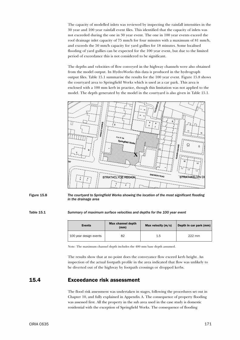
CIRIA C635 171

The capacity of modelled inlets was reviewed by inspecting the rainfall intensities in the

30 year and 100 year rainfall event files. This identified that the capacity of inlets was

not exceeded during the one in 30 year event. The one in 100 year events exceed the

roof drainage inlet capacity of 75 mm/h for four minutes with a maximum of 81 mm/h,

and exceeds the 50 mm/h capacity for yard gullies for 18 minutes. Some localised

flooding of yard gullies can be expected for the 100 year event, but due to the limited

period of exceedance this is not considered to be significant.

The depths and velocities of flow conveyed in the highway channels were also obtained

from the model output. In HydroWorks this data is produced in the hydrograph

output files. Table 15.1 summarise the results for the 100 year event. Figure 15.8 shows

the courtyard area to Springfield Works which is used as a car park. This area is

enclosed with a 100 mm kerb in practice, though this limitation was not applied to the

model. The depth generated by the model in the courtyard is also given in Table 15.1.

Figure 15.8 The courtyard to Springfield Works showing the location of the most significant floodingin the drainage area

Table 15.1 Summary of maximum surface velocities and depths for the 100 year event

Note: The maximum channel depth includes the 400 mm base depth assumed.

The results show that at no point does the conveyance flow exceed kerb height. An

inspection of the actual footpath profile in the area indicated that flow was unlikely to

be diverted out of the highway by footpath crossings or dropped kerbs.

15.4 Exceedance risk assessment

The flood risk assessment was undertaken in stages, following the procedures set out in

Chapter 10, and fully explained in Appendix A. The consequence of property flooding

was assessed first. All the property in the sub area used in the case study is domestic

residential with the exception of Springfield Works. The consequence of flooding

X

EventsMax channel depth

(mm)Max velocity (m/s) Depth in car park (mm)

100 year design events 82 1.5 222 mm

property situated below the level of the adjacent highway or with cellars was assessed first.

This was done by comparing the modelled levels of sewer surcharging with the property

base level. Each individual property was assigned a consequence level using the level

criteria set out in Table 10.8. This was done for both the 30 year and 100 year events.

The probability of flooding different property was assessed for each event based on the

proximity to an identified flood pathway by inspection from the plans. Combining

probability and consequence using a matrix similar to that in Figure 10.13 enabled a

comparative risk score for property to be established. None of the properties gave a

high risk score, with the medium high only being assigned to a small number or

properties in Muir Street and Arnold Avenue.

A review of maximum velocities (see Table 15.1) showed that there was no additional

risk associated with velocities. The associated risk scores for property are shown in

Figure 15.9 for the 100 year event.

Health and safety aspects were also reviewed by comparing modelled flow velocities

and depths in surface pathways (see Table 14.1). However none of the values recorded

were significant enough to warrant a risk score.

The most important result from the modelling and risk assessment were from the

Springfield Works compound. This showed a flood level of 232 mm for the 100 year event,

which overtops the kerb level and would cause flooding to the works. This was confirmed

by the event of July 2002 when there was considerable flood damage to the works.

15.5 Solution development

Flooding in the Springfield Works courtyard causes a problem for both the 30 year and

100 year event as levels exceed the 100 mm kerb height of the car park and enter the

works. Options for flood alleviation focused on two key alternatives:

� providing additional storage in the sewer system to protect property from flooding

for the 30 year event

� increased capacity through the provision of a new sewer connected to the Kelvin

Valley trunk sewer.

The storage option proved impractical due to the unavailability of land in the vicinity

of Springfield Works to construct a storage tank. The relief sewer option was created as

a potential solution.

To connect to the Kelvin Valley trunk sewer and alleviate the 30 year flood event, a

450 mm new sewer is required along the line shown in Figure 15.10. Surface

conveyance along highways will still occur with this solution. For surface flooding to be

removed for the 100 year event, a 750 mm sewer is required. However, modelling the

effects of the 100 year event shows that the water level in the car park at Springfield

Works remains below kerb level and drains away at the end of the storm. The area acts

as temporary surface storage for exceedance flows without risk of flooding the works.

Although velocities and depths in surface pathways increase for the 100 year event,

they still remain within the design requirements.

The 450 mm new sewer to convey flows to the Kelvin Valley trunk sewer so remains the

preferred option.

CIRIA C635172

Figure 15.9 Exceedance flood risk assessment for 100 year event

Figure 15.10 Solutions model with 100 year event showing flood risk

15.6 Impact on downstream systems

For the 100 year event all exceedance flows are conveyed on the surface to the

courtyard of the Springfield works, as described above. Flows are stored temporarily at

this point and are discharged to the new 450 mm sewer that transfers flow to the

Kelvin Valley trunk sewer to the north west of the area, as shown in Figure 15.10. A

model of the Kelvin Valley trunk sewer was available, and the additional flows were

input into this. The results show that they do not cause a significant deterioration in

the performance of the trunk sewer. A further solution was tested, using a 600 mm

sewer, which was the size required to convey the 100 year flood flow. This did cause

some noticeable deterioration in the Kelvin Valley trunk sewer performance.

CIRIA C635 173

X

X

CIRIA C635174

Part D Appendices

A1 Modelling exceedance

A1.1 Surface flood pathways

There are various methods used to represent surface flood pathways in network

models. Where the software tool does not explicitly include an algorithm for modelling

such pathways, it is common practice for the user to specify additional links between

nodes using an open channel link. There are two possible alternatives:

� surface channel links of the major system connect between the existing nodes of the

minor system

� a separate system of nodes and links are used to specify the major system, with

appropriate interconnecting links between the nodes of the two systems.

The former has the advantage of requiring the minimal modification to the minor

system network. However it constrains the major system in that it can only connect

between the minor system nodes (though some applications will allow the creation of

additional nodes where necessary). Also it is not usually possible to assign separate

contributing areas to the major system with this method.

The latter, which is illustrated in Figures 9.6 and 15.7, has the disadvantage that

additional network modelling is required. However, the major system layout is no

longer constrained to that of the minor system, and the links between the two sets of

nodes can be used to accurately model transfers of flow between the two systems. Care

should be taken with the dummy manholes specified in this method as they may

confuse the algorithms in the software into performing additional and inappropriate

calculations in relation to manhole head losses and additional storage volume.

The accuracy of modelling the surface pathway section will also depend on the

algorithms used to define the open channel model. Some software allows compound

channel shapes to be represented, so that flow within and without the highway can be

represented. Others restrain the user to simple rectangular sections, which should be

used with caution.

The facilities for viewing output also vary between different software packages. Where

the results can be shown graphically and in real time, in 3D format, the user can gain a

greater understanding of the movement of floodwater in the drainage area (Figure A1).

CIRIA C635186

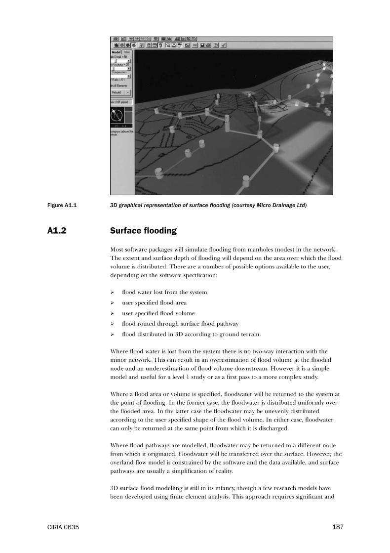
Figure A1.1 3D graphical representation of surface flooding (courtesy Micro Drainage Ltd)

A1.2 Surface flooding

Most software packages will simulate flooding from manholes (nodes) in the network.

The extent and surface depth of flooding will depend on the area over which the flood

volume is distributed. There are a number of possible options available to the user,

depending on the software specification:

� flood water lost from the system

� user specified flood area

� user specified flood volume

� flood routed through surface flood pathway

� flood distributed in 3D according to ground terrain.

Where flood water is lost from the system there is no two-way interaction with the

minor network. This can result in an overestimation of flood volume at the flooded

node and an underestimation of flood volume downstream. However it is a simple

model and useful for a level 1 study or as a first pass to a more complex study.

Where a flood area or volume is specified, floodwater will be returned to the system at

the point of flooding. In the former case, the floodwater is distributed uniformly over

the flooded area. In the latter case the floodwater may be unevenly distributed

according to the user specified shape of the flood volume. In either case, floodwater

can only be returned at the same point from which it is discharged.

Where flood pathways are modelled, floodwater may be returned to a different node

from which it originated. Floodwater will be transferred over the surface. However, the

overland flow model is constrained by the software and the data available, and surface

pathways are usually a simplification of reality.

3D surface flood modelling is still in its infancy, though a few research models have

been developed using finite element analysis. This approach requires significant and

CIRIA C635 187

detailed digital terrain data and substantial computing power. However it sets out the

likely route for future software development. A simpler approach to allowing for three

dimensional ground effects is to use a “rolling ball” algorithm to identify a surface flood

pathway. The “rolling ball” algorithm works with a digital terrain model and identifies

the line of greatest slope in each grid. These are then joined together to form a surface

flood pathway. This will convey flow to a low point, or to another part of the minor

system, as shown in Figure A1.2.

Figure A1.2 Overland flow paths identified with “rolling ball” algorithm (courtesy Wallingford Software)

Some software enables the user to assess the direction where above ground flows may

split when flow reaches a crest. This accounts for flow that may split in several different

directions from a single source.

A1.3 Modelling inlet capacity

As explained in Chapter 9, the capacity of different drainage inlets is limited, and this

can be important in extreme events. Some software explicitly allows for modelling the

restrictive effects of inlet capacity. This may be done by applying a throttle to the inlet,

CIRIA C635188

and including a notional reservoir to allow for subsequent storage on the surface

upstream. This is illustrated in Figure A1.3, where the algorithm for a flooded node is

adapted to restrict the flow passing in from the surface.

Normally, each individual area contributing to a gully would not be represented, rather

they would be grouped together to represent a number of areas draining to a notional

gully.

Figure A1.3 Model of gully inlet (courtesy Wallingford Software)

A1.4 Modelling flood risk

Some software packages will perform additional calculations to estimate the direct flood

risk to property. Risk will depend on the likelihood that property will flood, and the

consequence if it floods. The likelihood of flooding depends on two factors: the level of

the property in relation to the level of surcharging in the minor system, and the

proximity of the property to surface flood paths in areas of flooding. This is illustrated

in Figure A1.4. The figure also illustrates that property below the level of the minor

system, or with a cellar, may flood even where no surface flooding is indicated at the

node of the minor system.

The consequence will depend on the depth to which the property is flooded which is

usually determined by the local depth of surface flooding, as illustrated in Figure A1.4.

A risk score can be developed by combining these two factors. Results can be indicated

on background mapping using GIS, as illustrated in Figure A1.7.

Some software adopts a sensitivity analysis approach that includes the potential of

climate change combined with the ability to model watercourses and rural, and urban

runoff. This gives a holistic approach to the prediction of flood pathways and flood

levels.

CIRIA C635 189

Figure A1.4 Property below level of minor system, showing flooding due to sewer surcharging

Figure A1.5 Property with cellar, showing flooding due to sewer surcharging

Figure A1.6 Property above level of minor system showing flooding due to local surface flooding

A1.5 Further guidance

It is not practical to give detailed guidance on individual software packages here.

Practitioners are advised to seek further guidance from the suppliers of such software

or to use help functions provided.

CIRIA C635190

Figure A1.7 Flood risk scoring at the level of individual property (courtesy MWH)

CIRIA C635 191

A2 Exceedance flow at highway gully inlets

The contents of this appendix are based on Highways Agency report HA102/00,

Spacing of highway gullies (Highways Agency, 2000)

The design of gully inlets is based on the knowledge that a proportion of flow bypasses

the gully grating under design conditions and continues along the channel of the

highway. A gully receives flow from its local contributing area plus a proportion of the

flow from upstream areas. It passes a proportion of this total flow onto the next gully

downstream. Ultimately the excess flow is collected by an additional gully at the low

spot. It is appreciated that highway drainage is based on the premise that the highway

acts as a drainage channel conveying major system flow.

With extreme events the flow in the highway channel will increase considerable.

However, this does not significantly affect the efficiency of the gully grating (see Table

A2.1), providing that the width of flow in the highway channel is not excessive (not

>1.5 m). Even where efficiencies are reduced due to poor maintenance highway gullies

can still achieve a steady state condition where the inflow to a group of gullies equals

the runoff from the contributing areas.

When assessing the effect of extreme events on highway drainage, the engineer needs

to consider the major system flow in the highway channel to determine whether the

depth or width of flow is such that a significant proportion of flow may be diverted

from the channel and ultimately not collected by the highway gullies. Such diverted

flow would become the exceedance flow.

However, using the methodology set out in Appendix 2, even with rainfall intensities

up to 300 mm/hr, and using typical contributing areas, it is unlikely that depth of flow

will be greater than 100 mm.

The flow bypassing a highway gully is shown in Figure A2.1 and represented by

Equation A2.1.

Figure A2.1 Flow split at highway gully inlet

The flow entering the gully, Qi (m³/s), is defined by the gully efficiency ç, and is given

by the equation.

(A2.1)

CIRIA C635192

where: η = m

Q = flow n highway channel approaching the gully

Gd = gully factor defined by the gully grating geometry

H = average depth of flow in the gully channel

m = factor to allow for maintenance

Note that a suitable maintenance factor for design would be 1 or 0.9, and a minimum

value used for exceedance conditions 0.7 (assumes worse maintenance).

It follows that the flow by-passing the gully is

(A2.2)

Qr is the flow (m³/s) collected from the contributing area to each gully, and is given by

the Rational equation,

(A2.3)

where:

Ae = contributing area as defined by Figure A2.2 (ha)

i = mean rainfall intensity (mm/hr) for 5 min duration

Figure A2.2 Effective area contributing to flow in channel - note that ç is calculated at the design flow

Q is also the flow conveyed in the highway channel (m³/s), made up of Qr + Qb, and is

related to the width and depth of flow by the Manning Equation

(A2.4)

where:

AF = cross-sectional area of flow in channel (m²)

R = hydraulic radius = AF/P (m)

P = wetted perimeter of flow section (m)

sL = average longitudinal slope of highway

n = Manning roughness for highway surface

CIRIA C635 193

( )100 – Gd ( )Q

H

Figure A2.3 shows the cross section of flow in the channel.

Figure A2.3 Cross-section of flow in the channel

It can be shown that:

and (A2.5)

where:

Example: For an urban road with gullies designed for a one year return period rainfall,

the exceedance flow for the 30 year rainfall may be calculated as follows.

Data:

Gully spacing = 12.4 m

Effective width of contributing area = 6.5 m

Contributing area = 0.00806 ha

Longitudinal slope sL = 1 in 40 (0.025)

Crossfall = 1 in 33 (0.030)

Maintenance factor for design = 1

Maintenance factor for exceedance calculation = 0.7

Design rainfall intensity for five min duration and annual probability of 1.0 = 55

mm/hr

Exceedance rainfall intensity of five min duration and annual probability of 0.02 = 148

mm/hr

CIRIA C635194

Runoff from contributing area per gully =2.78 × 0.00806 × 55 = 1.23 l/s for the design

event and 2.78 × 0.00806 × 148 = 3.32l/s for the exceedance event.

For the design conditions make a first estimate of gully efficiency using a channel flow

equal to the runoff.

From Table A2.1, K1 = 0.173 so that the depth of flow in the channel is:

so that the gully efficiency

Under steady state conditions the gully inlet flow Qi equals the runoff from the

contributing area Qr = 1.23l/s.

The channel flow and the by-pass flow is 0.06 l/s

Reworking the above calculation with a flow of 1.29 rather than 1.23 l/s leaves the gully

efficiency unchanged at 95 per cent.

For the exceedance conditions, assume initially that the gully efficiency can be derived

from the design value as:

As explained above, the inflow to the gully equals the runoff = 3.32l/s so that the

channel flow becomes

For a channel flow of 5.03 l/s the depth of flow in the channel now becomes

The gully efficiency is now:

CIRIA C635 195

The channel flow is now reworked as:

and the by-pass flow is 2.12 l/s

The depth of flow in the highway channel may now be calculated using Equation A2.5.

For a cross-fall of one in 33, the width of flow becomes 0.825 m, which is within the

required 1.5 m.

The flow entering each gully is 3.32 l/s which is well below the limiting capacity of 10 l/s

for a gully with a 100 mm outlet. So it follows that even where drop kerbs exist, it is

extremely unlikely that any of the extreme event runoff will result in exceedance flow

due to the capacity of the gully inlets.

CIRIA C635196

CIRIA C635 197

Table A2.1 Values of K1

n sL Sc K1 n sL Sc K1

0.015 0.010 0.005 0.104 0.015 0.035 0.005 0.081

0.015 0.010 0.010 0.135 0.015 0.035 0.010 0.105

0.015 0.010 0.015 0.157 0.015 0.035 0.015 0.122

0.015 0.010 0.020 0.176 0.015 0.035 0.020 0.136

0.015 0.010 0.025 0.191 0.015 0.035 0.025 0.148

0.015 0.010 0.030 0.205 0.015 0.035 0.030 0.159

0.015 0.010 0.035 0.217 0.015 0.035 0.035 0.168

0.015 0.010 0.040 0.229 0.015 0.035 0.040 0.177

0.015 0.010 0.045 0.239 0.015 0.035 0.045 0.186

0.015 0.010 0.050 0.249 0.015 0.035 0.050 0.193

0.015 0.015 0.005 0.096 0.015 0.040 0.005 0.079

0.015 0.015 0.010 0.125 0.015 0.040 0.010 0.102

0.015 0.015 0.015 0.146 0.015 0.040 0.015 0.119

0.015 0.015 0.020 0.163 0.015 0.040 0.020 0.133

0.015 0.015 0.025 0.177 0.015 0.040 0.025 0.144

0.015 0.015 0.030 0.190 0.015 0.040 0.030 0.155

0.015 0.015 0.035 0.201 0.015 0.040 0.035 0.164

0.015 0.015 0.040 0.212 0.015 0.040 0.040 0.173

0.015 0.015 0.045 0.222 0.015 0.040 0.045 0.181

0.015 0.015 0.050 0.231 0.015 0.040 0.050 0.188

0.015 0.020 0.005 0.091 0.015 0.045 0.005 0.077

0.015 0.020 0.010 0.119 0.015 0.045 0.010 0.100

0.015 0.020 0.015 0.138 0.015 0.045 0.015 0.116

0.015 0.020 0.020 0.154 0.015 0.045 0.020 0.130

0.015 0.020 0.025 0.168 0.015 0.045 0.025 0.141

0.015 0.020 0.030 0.180 0.015 0.045 0.030 0.151

0.015 0.020 0.035 0.191 0.015 0.045 0.035 0.161

0.015 0.020 0.040 0.201 0.015 0.045 0.040 0.169

0.015 0.020 0.045 0.210 0.015 0.045 0.045 0.177

0.015 0.020 0.050 0.219 0.015 0.045 0.050 0.184

0.015 0.025 0.005 0.088 0.015 0.050 0.005 0.075

0.015 0.025 0.010 0.114 0.015 0.050 0.010 0.098

0.015 0.025 0.015 0.133 0.015 0.050 0.015 0.114

0.015 0.025 0.020 0.148 0.015 0.050 0.020 0.127

0.015 0.025 0.025 0.161 0.015 0.050 0.025 0.139

0.015 0.025 0.030 0.173 0.015 0.050 0.030 0.149

0.015 0.025 0.035 0.183 0.015 0.050 0.035 0.158

0.015 0.025 0.040 0.193 0.015 0.050 0.040 0.166

0.015 0.025 0.045 0.202 0.015 0.050 0.045 0.174

0.015 0.025 0.050 0.210 0.015 0.050 0.050 0.181

0.015 0.030 0.005 0.085 0.015 0.055 0.005 0.074

0.015 0.030 0.010 0.110 0.015 0.055 0.010 0.096

0.015 0.030 0.015 0.128 0.015 0.055 0.015 0.113

0.015 0.030 0.020 0.143 0.015 0.055 0.020 0.125

0.015 0.030 0.025 0.156 0.015 0.055 0.025 0.136

0.015 0.030 0.030 0.167 0.015 0.055 0.030 0.146

0.015 0.030 0.035 0.177 0.015 0.055 0.035 0.155

0.015 0.030 0.040 0.186 0.015 0.055 0.040 0.163

0.015 0.030 0.045 0.195 0.015 0.055 0.045 0.170

0.015 0.030 0.050 0.203 0.015 0.055 0.050 0.178

A3 Conveyance in surface flood pathways

A3.1 Introduction

The design of surface flood pathways is set out in Chapters 9 and 11 in Part B of the

guidance. The purpose of this appendix is to give supplementary information on

typical surface flood channel sections.

A3.2 Flood pathway channels

The following figures show some typical surface flood pathways encountered in urban

areas. They are only intended to be indicative since the type, size and detail is infinite.

However they will give a good indication of typical dimensions and surface roughness.

Figure A3.1 Typical cross-section of flood pathway in a minor highway, showing surface conveyance fornon-extreme events

Figure A3.2 As Figure A3.1 but with exceedance flow contained within the highway channel.Note: The exceedance flow occupies the space between the free surface and the surface of the normal

drainage flow (shown dotted)

CIRIA C635198

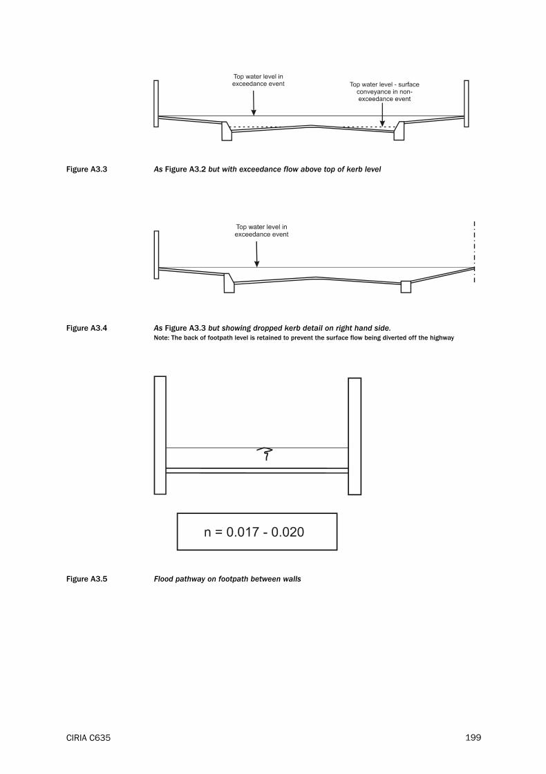
Figure A3.3 As Figure A3.2 but with exceedance flow above top of kerb level

Figure A3.4 As Figure A3.3 but showing dropped kerb detail on right hand side.Note: The back of footpath level is retained to prevent the surface flow being diverted off the highway

Figure A3.5 Flood pathway on footpath between walls

CIRIA C635 199

Figure A3.6 Flood pathway on footpath between grass banks

Figure A3.7 Flood pathway in rough cut ditch

Figure A3.8 Flood pathway in lined ditch

CIRIA C635200

A4 Assessment approach to determine

flood volumes and rates from SuDS

A4.1 Assessment approach

An analysis was carried out on the most relevant SuDS units to evaluate their

exceedance characteristics. The systems assessed were:

� pervious pavements

� swales

� infiltration systems.

The approach taken was to model the SuDS unit using a drainage modelling tool and

apply rainfall to a drainage area. Examination of the model results enables an

assessment of the hydraulic performance of the unit to be made, with peak flow rates

and volumes quantified when the capacity of the unit was exceeded.

The performance of a SuDS unit is a combination of rainfall event and the volume of

storage provided, so this analysis involved running a range of models. For example a

swale of the same shape and length receiving runoff from the same storm and

contributing surface area, will perform very differently when built with a slope of 1:20

compared with one of a slope of 1:200. The volume provided by the latter is greater

and provides a corresponding higher level of service.

The results provide an indication of the exceedance performance of the SuDS systems,

based on the various assumptions used in the analysis. Where these assumptions apply

fairly closely with the drainage system being designed, these results can be used to

provide an indication of the impact of rainfall exceedance and appropriate design

carried out to address these excess flows.

There are too many variables to provide this information for all drainage situations. A

generic indication of exceedance performance is provided in Appendix 5. This

appendix is aimed at providing a first order indication of performance as a number of

significant assumptions are made to enable this guidance to be developed.

A4.2 Hydrology

The hydrology of the country can be divided into eight categories by using the FSR

parameters M560 and rainfall ratio “r”. These parameters measure the 60 minute

rainfall depth of the storm with the probability of occurrence of 0.2 per year and the

ratio of the 60 minutes to the two-day event of the same probability of occurrence.

Figure D.1 illustrates these eight areas. Although FSR is generally accepted as having

been superseded by the Flood Estimation Handbook (FEH) (CEH, 1999), this figure

provides the simplest method of an overview of the hydrology across the country.

To minimise the analysis, rather than running eight different sets to represent all the

hydrological regions, two representative regions were chosen. The FSR parameters

selected for M560 and rainfall ratio “r” were 17 mm and 0.2 which generally describes

CIRIA C635 201

areas to the north and west of the country, and 20 mm and 0.4 which generally

describes the south and east.

However it is recognised that FEH and climate change together means that use of the

FSR rainfall would not be a conservative assumption for doing this assessment,

particularly for extreme events. The rainfall has been factored up to take account of

this.

Figure A4.1 FSR regions across the UK (courtesy HR Wallingford)

A4.3 Pervious pavement performance

Pervious pavements are normally built with 350 mm of granular fill to a specific stone size

mix. This provides around 30 per cent voids for water storage. High voids storage,

around 95 per cent, can also be constructed using plastic crate type systems. These can be

used for both smaller depths than 350 mm as well as depths of up to a few metres. The

standard granular construction with 30 per cent voids has been selected for analysis.

CIRIA C635202

The volume of storage is large even with respect to large rainfall events, and so the

analysis also looked at the use of the pavement to provide storage for adjacent

impermeable areas, and reflect common practice. The throttle rates used were not

modified in assessing the extra demands made by these areas, though in practice

hydraulic discharge criteria would probably increase proportionately.

Table A4.1 Summarises the assumptions used for assessing the hydraulic performance

of pervious pavements and their impact on the major system.

Table A4.1 Pervious pavements – modelling assumptions

* These outflows could be considered to be either throttles on the outlet or an infiltration capacitybelow the car park. These infiltration rates are well below the values which would be consideredappropriate for use of soakaway devices.

A4.3.1 Results

The results of the analysis were evaluated for both the maximum “spill” volume and

the peak rate of flow when it became full and overflowed. The maximum duration

selected was a 12 hour event, though it should be noted that these flow rates and

volumes sometimes increase for longer duration events. Figures 9.6 and 9.7 summarise

the results and shows that overflow never takes place for any event even with the

smallest throttle rate when the car park does not serve additional impermeable areas.

When it serves an addition of 1 ha it becomes surcharged and overflow takes place for

extreme long duration events. The northern climate with its greater depths of long

duration storms shows a significant reduction in performance compared with the

southern climate. Where the additional area is limited to 1 ha, only the 200 year event

in the south spills, while in the north, the maximum overflow rate is 61 l/s for a 200

year event. However it should be noted that the 30 year event is catered for without

flooding for all scenarios in the south, but causes a small amount of exceedance flow in

the north.

This trend is extended when 2 ha of additional area is drained to the pavement. The

maximum overflow rate for this situation is 95 l/s which is from a 12 hour 200 year

event.

CIRIA C635 203

Pervious pavement Characteristics and scenarios

Physical pavement construction

characteristics

1 ha area

350 mm deep

30 per cent voids

Horizontal

Outflow from the pavement * 1, 2, 5 and 10 l /s/ha

(0.36 – 3.6 mm/hr)

Inflow to the pavement 100 per cent runoff with 5 mm depression storage

a) Car park area only

b) 1 ha of additional paved area

c) 2 ha of additional paved area

Hydrology and climate change factors 20/0.4 (south) and 17/0.2 (north)

1 to 10 year (factor 1.1)

30 and 50 year (factor 1.2)


1 – 12 hour events design storms

Similarly, Figure 9.15 and Figure 9.16 show the maximum volumes of spill. The

additional 2 ha of impermeable area for the 200 year event generates an overflow

volume of over 1100 m³ in the south rising to nearly 2000 m³ in the north. These large

volumes reflect the very low limit of discharge applied in this case.

A4.3.2 Application of results and conclusions

The four Figures of 9.6 to 9.10 provide a simple way to assess the exceedance flow

from a pervious pavement which has a storage depth of around 120 mm for a range of

limiting outflow discharge rates and impermeable area served. The following general

advice can also be derived from these results.

� pervious pavements with this depth of storage will never cause a rainfall

exceedance problem for events with a probability of occurrence less than 0.005 in

any year until it is used to provide storage for an additional impermeable area that

is at least equal in extent to that of the pervious pavement

� where the extent of the additional surcharge area is significantly greater than the

area of the pervious pavement, the volume of runoff, which cannot be catered for

within the unit, becomes large and would need specific consideration for long

duration extreme events (12 to 48 hours). The limiting discharge would need to be

significantly greater than the range used in this analysis to eliminate this flood

volume

� the rate of “overflow” is unlikely to ever cause a significant flood flow depth in

terms of the conveyance in the major system as the events that cause exceedance

are not short sharp high intensity storms.

To obtain values for other arrangements of storage provision, hydrological regions,

outflow rates and contributing areas, it is necessary to produce a model of the system.

However a generic “look-up” method is provided in Appendix 5. It has been derived

based on a number of simplifying assumptions which enables a first order estimate of

the exceedance characteristics for any SuDS system.

A4.4 Swale performance

Swales are still not frequently used in UK and current design criteria are only related

to erosion control, pollutant removal and maintenance needs. There are a number of

different types of swale configurations (under-drained, standard conveyance, partial

storage with overflow etc) which means that there are endless possibilities for the

hydraulic design of these units. Hydraulic criteria relating to hydraulic performance

has yet to be defined and accepted nationally. Current design guidance suggests that

swales would not provide a level of service greater than a return period of 10 years and

that road drainage design only requires around a one year level of service. Slopes

across a site and the different lengths of swale, which are needed to fit into the road

layout, makes the performance of each swale length unique. This means that simple

guidance on exceedance behaviour is very difficult to derive.

The common cross-section often used to describe the requirements of a swale is shown

in Figure A4.2. The performance of a swale is related to the outflow characteristics

(outlet size and infiltration along its length), the inflow (the area generating runoff from

rainfall) and the volume of storage in the swale before it fills and starts spilling down the

road. This volume is not a function of the length of the swale, but the proportion which

is below the level of the top of the swale at the downstream end. For steep swales this

can be quite a short length. At 1:20 gradient, the bottom of the swale eight metres from

the downstream end is the same level as the top of the swale if the depth is 400 mm.

CIRIA C635204

Guidance on exceedance design is through the provision of information on

performance relating for a range of combinations of slope and length of swale assuming

a standard cross-section. This provides a good understanding of the level of service

provided by swales and the typical range of flow rates and volumes that can occur

during extreme events. General guidance advice is drawn from the results.

Assumptions are needed for deriving an understanding of level of service and

exceedance behaviour for the following elements:

� contributing area

� gradient of the swale

� length of the swale

� outflow control from the swale.

Figure A4.2 Swale cross-section

A4.4.1 Contributing area

The effective area contributing runoff is assumed to be a half road width (3.5 m)

together with an allowance of 1.5 m to allow for the bottom of the swale and some

adjacent runoff. Runoff is assumed to be 100 per cent. The length of road is assumed

to be the same as the length of the swale.

A4.4.2 Gradient of the swale

Gradients analysed range from 1:20 to 1:250. Design guidance (Martin et al, 2000a)

suggests that 1:17 should not be exceeded, though figures ranging from 1:10 to 1:28

are also suggested in other SuDS literature. This maximum gradient is set to reduce

the risk of erosion, ensure a degree of treatment and reduce the collection of sediment

at the bottom end of the channel. Swales flatter than 1:100 may have problems

draining. However the current trend towards bio-retention means that in many cases,

flatter gradients may be considered to be quite desirable.

A4.4.3 Length of the swale

Although pollution design criteria includes a suggested minimum length of 30 m with a

preference for 60 m, in a residential estate the length of a swale would range between

20 m and 100 m before it has to terminate. At this point it would either pass under the

obstruction/road into another swale or connect to a carrier pipe in the road. This range

has been used to assess swale performance.

CIRIA C635 205

A4.4.4 Outflow control from the swale

In this analysis infiltration is assumed not to take place on the basis that the reduction

in volume lost by infiltration from an extreme event is small relative to the total runoff

volume. Swales are normally served by an outfall pipe which passes to a carrier sewer.

Based on the normal water company requirements of a minimum pipe size of 150 mm

diameter, an outflow rate of 15 l/s has been assumed. At the other extreme the worst

case scenario is for a blocked outlet. These two outflow rates have been used together

with an intermediate flow rate of 7.5 l/s to provide additional information (see Table

A4.2).

As for the pervious pavements, the assessment provides peak “overflow” rates when the

swales are filled and spills take place, and also the maximum volume spilled. Design

events ranging from one to 200 year return period have been used.

Table A4.2 Swale – modelling assumptions


As for pervious pavements, the maximum duration selected was a 12 hour event. Tables

9.5 and 9.6 summarise the output on maximum spill rates and total volumes

respectively for the 100 m swale for southern UK rainfall. Tables A4.3 to A4.14

illustrate the results for northern and southern rainfall for shorter swales.

These graphs can be used by interpolation to determine approximate flood flow rates

and flood volumes. Where swales are proposed to be built with different profiles or

with longer runs, either models will need to be built to predict their exceedance

performance or Appendix 5 can be used to obtain a first order estimate of their flood

characteristics.

CIRIA C635206

Swale Characteristics and scenarios

Swale shape 1:4 side slope

400 mm deep

1 m base width

Lengths 20 m, 50 m, 100 m

Gradients 1:20, 1:50, 1:100, 1:250

Outflow from the swale 0, 7.5 and 15 l/s

Inflow to the swale 100 per cent runoff

5.0 m road width


one to 10 year (factor 1.1)



one to 12 hour events design storms

six extreme events from a time series

Table A4.3 Overflow rate (l/s) from 20 m long swale system – south

Table A4.4 Overflow rate (l/s) from 20 m long swale system – north



CIRIA C635 207


Gradient (m/m)

Return period

0.05 0.02 0.010.00

40.05 0.02 0.01

0.00

40.05 0.02 0.01 0.004

1 0 0 0 0 0 0 0 0 0 0 0 0

10 0 0 0 0 0 0 0 0 0.1 0 0 0

30 0 0 0 0 0 0 0 0 0.4 0 0 0

100 0 0 0 0 0 0 0 0 1.6 0.1 0 0

200 0 0 0 0 0 0 0 0 2.7 0.3 0 0


Gradient (m/m)

Return period

0.05 0.02 0.010.00

40.05 0.02 0.01

0.00

40.05 0.02 0.01 0.004

1 0 0 0 0 0 0 0 0 0 0 0 0

10 0 0 0 0 0 0 0 0 0 0 0 0

30 0 0 0 0 0 0 0 0 0 0 0 0

100 0 0 0 0 0 0 0 0 0 0 0 0

200 0 0 0 0 0 0 0 0 0 0 0 0


Gradient (m/m)

Return period

0.05 0.02 0.010.00

40.05 0.02 0.01

0.00

40.05 0.02 0.01 0.004

1 0 0 0 0 0 0 0 0 0.2 0 0 0

10 0 0 0 0 0 0 0 0 2.0 0.4 0 0

30 0 0 0 0 0 0 0 0 6.2 1.7 0 0

100 0 0 0 0 0 0 0 0 14.8 5.9 0.9 0

200 0 0 0 0 0 0 0 0 20 9.7 1.7 0


Gradient (m/m)

Return period

0.05 0.02 0.010.00

40.05 0.02 0.01

0.00

40.05 0.02 0.01 0.004

1 0 0 0 0 0 0 0 0 0.8 0.1 0 0

10 0 0 0 0 0 0 0 0 2.2 1.2 0 0

30 0 0 0 0 0 0 0 0 4.9 2.4 0.6 0

100 0 0 0 0 0 0 0 0 9.6 5.2 2.0 0

200 0 0 0 0 0 0 0 0 12.5 8.6 2.9 0



Table A4.9 Overflow volume (m³) from 20 m long swale system – south

Table A4.10 Overflow volume (m³) from 20 m long swale system – north

CIRIA C635208


Gradient (m/m)

Return period

0.05 0.02 0.010.00

40.05 0.02 0.01

0.00

40.05 0.02 0.01 0.004

1 0 0 0 0 0 0 0 0 2.7 0.8 0 0

10 0 0 0 0 0 0 0 0 14.4 5.6 1.1 0

30 0 0 0 0 6.5 0 0 0 27 14.3 3.5 0

100 15.4 0 0 0 31.7 8.7 0 0 44.5 30.8 11.8 0.6

200 29.3 0 0 0 41 20.9 0 0 51.4 39.8 18.8 1.7


Gradient (m/m)

Return period

0.05 0.02 0.010.00

40.05 0.02 0.01

0.00

40.05 0.02 0.01 0.004

1 0 0 0 0 0 0 0 0 2.6 1.8 0.2 0

10 0 0 0 0 0 0 0 0 9.3 4.9 2.4 0

30 0 0 0 0 0 0 0 0 15.6 10.6 5 0.4

100 0 0 0 0 9.6 0 0 0 26.3 20.1 10.6 2.6

200 0 0 0 0 18.2 0 0 0 31 24.9 16.8 4


Gradient (m/m)

Return period

0.05 0.02 0.010.00

40.05 0.02 0.01

0.00

40.05 0.02 0.01 0.004

1 0 0 0 0 0 0 0 0 0 0 0 0

10 0 0 0 0 0 0 0 0 0.4 0 0 0

30 0 0 0 0 0 0 0 0 2.2 0 0 0

100 0 0 0 0 0 0 0 0 4.8 0.7 0 0

200 0 0 0 0 0 0 0 0 6.3 2.1 0 0


Gradient (m/m)

Return period

0.05 0.02 0.010.00

40.05 0.02 0.01

0.00

40.05 0.02 0.01 0.004

1 0 0 0 0 0 0 0 0 0 0 0 0

10 0 0 0 0 0 0 0 0 1.9 0 0 0

30 0 0 0 0 0 0 0 0 4.1 0 0 0

100 0 0 0 0 0 0 0 0 7.2 3.1 0 0

200 0 0 0 0 0 0 0 0 8.9 4.7 0 0

Table A4.11 Overflow volume (m³) from 50 m long swale system – south

Table A4.12 Overflow volume (m³) from 50m long swale system – north

Table A4.13 Overflow volume (m³) from 100m long swale system – south

Table A4.14 Overflow volume (m³) from 100m long swale system – north

CIRIA C635 209


Gradient (m/m)

Return period

0.05 0.02 0.010.00

40.05 0.02 0.01

0.00

40.05 0.02 0.01 0.004

1 0 0 0 0 0 0 0 0 0 0 0 0

10 0 0 0 0 0 0 0 0 0.4 0 0 0

30 0 0 0 0 0 0 0 0 2.2 0 0 0

100 0 0 0 0 0 0 0 0 4.8 0.7 0 0

200 0 0 0 0 0 0 0 0 6.3 2.1 0 0


Gradient (m/m)

Return period

0.05 0.02 0.010.00

40.05 0.02 0.01

0.00

40.05 0.02 0.01 0.004

1 0 0 0 0 0 0 0 0 4.2 0.6 0 0

10 0 0 0 0 0 0 0 0 10.4 6.7 0 0

30 0 0 0 0 0 0 0 0 15.9 12.3 4.3 0

100 0 0 0 0 0 0 0 0 23.8 20.2 12.1 0

200 0 0 0 0 0 0 0 0 28 24.3 16.3 0


Gradient (m/m)

Return period

0.05 0.02 0.010.00

40.05 0.02 0.01

0.00

40.05 0.02 0.01 0.004

1 0 0 0 0 0 0 0 0 8.7 4.9 0 0

10 0 0 0 0 0 0 0 0 18.8 15 6.9 0

30 0 0 0 0 0.7 0 0 0 27.9 24.1 16.1 0

100 1.3 0 0 0 5.4 1.5 0 0 41.1 37.3 29.2 5.8

200 3.4 0 0 0 8.1 4.4 0 0 48.4 44.5 36.5 13.8


Gradient (m/m)

Return period

0.05 0.02 0.010.00

40.05 0.02 0.01

0.00

40.05 0.02 0.01 0.004

1 0 0 0 0 0 0 0 0 14 10.2 2.2 0

10 0 0 0 0 0 0 0 0 26.3 22.5 14.4 0

30 0 0 0 0 0 0 0 0 37.4 33.6 25.6 2.1

100 0 0 0 0 1.8 0 0 0 53.1 49.3 41.3 17.9

200 0 0 0 0 4.5 0 0 0 61.5 57.7 49.6 26.2

A4.5 Infiltration system performance

Infiltration trenches and soakaways can be designed accommodate rainfall up to a 10

year return period. A design methodology is outlined in CIRIA R156. They are often

filled with granular material, with the system designed to infiltrate surface water into

the ground.

The critical issue for infiltration systems (as with all outlet rate assumptions for these

SuDS units) is the rate of infiltration into the subsurface material. Clay-like soils allow

very little infiltration whereas a sandy soil allows high levels of infiltration. Infiltration

rates normally range from 5 × 10-4 mm/s for a soil with marginal infiltration capacity to

1 × 10-2 mm/s for a soil with a relatively good infiltration capacity.

As for the pervious pavement and swales, the analysis provides an assessment of peak

flood flows when the infiltration system has filled and the maximum volume generated.

The test characteristics are shown in Table A4.15.

Table A4.15 Infiltration system – test characteristics


Table A4.16 and A4.17 summarise the maximum flood flow rates and maximum flood

volumes respectively for the infiltration trench for southern UK rainfall. Figures for the

northern UK rainfall are not provided as the design of an infiltration trench would

largely take into account the difference in performance for the various return periods.

These graphs can be used by interpolation or limited extrapolation for any infiltration

rate and return period rainfall to determine approximate flood flow rates and flood

volumes. Where infiltration units are used with very different infiltration rates or

designed to a criterion other than a 10 year return period, either models will need to

be built to predict their exceedance performance or Appendix 5 can be used to obtain a

first order estimate of their flood characteristics.

CIRIA C635210

Infiltration system Characteristics and scenarios

Design criteria 10 year return period

30 per cent void ratio

Outflow No pass forward flow

Inflow to the system 50 m² roof area × 50 houses per hectare

(Total catchment = 2500 m² per hectare)

Infiltration rates 5 × 10-4 mm/s – marginal

1 × 10-2 mm/s – good


one to 10 year (factor 1.1)



Table A4.16 Overflow rate (l/s) from infiltration system

Table A4.17 Overflow volume (m³) from infiltration system

CIRIA C635 211

Location North South

Infiltration rate

(mm/hr)

Return period

1.8 3.6 36 1.8 3.6 36

10 1.3 2.4 0 8.1 9.6 1.1

30 10.8 14.5 9.6 17.1 16.1 16.5

100 20 18.8 17.6 19.5 21.5 18.2

200 22.3 24.7 22.5 25.2 26.5 22.5

Location North South

Infiltration rate

(mm/hr)

Return period

1.8 3.6 36 1.8 3.6 36

10 9.9 8.4 0 73.8 66.5 0.5

30 61.4 53.6 12.7 144.4 131.6 31.7

100 136.5 123.3 57 240.4 225.1 86

200 176.7 161.3 84.1 287.2 271.2 117.3

A5 Generic guidance on assessing flood

volumes and rates from SuDS

The results of the analysis of the various SuDS units in Appendix 4 provide an outline

for the performance of SuDS systems. There is difficulty in comparing the units

because the performance is a function of the assumptions made regarding the design of

the unit. The results provide a guide as to their performance and they can be used to

determine the maximum flood flows if the assumptions used apply to the case being

considered.

A generic method has been developed to enable the performance of a SuDS unit to be

predicted. This method allows the peak flood flow rate and total volume of flooding to

be estimated. Unfortunately the various aspects of head-discharge characteristics,

variable infiltration rates and attenuation of runoff makes the derivation of a generic

approach only approximate. It should be stressed that the range of assumptions that

has to be made in using this method, makes this approach only suitable as a first order

assessment of the situation. The estimate of flood volume will probably be more

accurate than the prediction of the peak flood flow rate.

In principle all drainage systems have a storage component together with an outflow

rate. Pipe systems have a relatively small storage component. However, in the case of

SuDS there is more emphasis on the storage element and specific allowance for this

should be made.

A5.1 Assumptions

A range of assumptions have been made in developing this assistance tool and these are

placed into three categories:

� inflow

� outflow

� storage.

These assumptions generally result in a conservative estimate of the storage required or

flood volume which will take place for any event. The results are too conservative for

units such as pervious pavements where the lag time needs to be taken into account.

Two versions have been produced; lagged and un-lagged. Units which have flow

passing through granular media, such as infiltration trenches and pervious pavements,

are based on the lagged method.

A5.1.1 Inflow

The assumptions used are that:

� runoff volume is generated assuming 100 per cent of the rainfall is effective

� rainfall intensity occurs at a constant intensity for each duration event

� runoff into the drainage unit occurs immediately.

CIRIA C635212

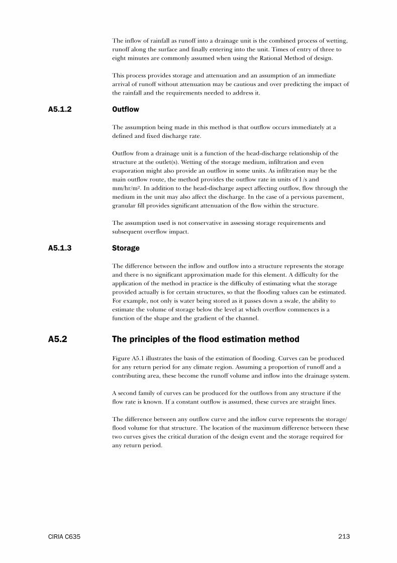
The inflow of rainfall as runoff into a drainage unit is the combined process of wetting,

runoff along the surface and finally entering into the unit. Times of entry of three to

eight minutes are commonly assumed when using the Rational Method of design.

This process provides storage and attenuation and an assumption of an immediate

arrival of runoff without attenuation may be cautious and over predicting the impact of

the rainfall and the requirements needed to address it.

A5.1.2 Outflow

The assumption being made in this method is that outflow occurs immediately at a

defined and fixed discharge rate.

Outflow from a drainage unit is a function of the head-discharge relationship of the

structure at the outlet(s). Wetting of the storage medium, infiltration and even

evaporation might also provide an outflow in some units. As infiltration may be the

main outflow route, the method provides the outflow rate in units of l /s and

mm/hr/m2. In addition to the head-discharge aspect affecting outflow, flow through the

medium in the unit may also affect the discharge. In the case of a pervious pavement,

granular fill provides significant attenuation of the flow within the structure.

The assumption used is not conservative in assessing storage requirements and

subsequent overflow impact.

A5.1.3 Storage

The difference between the inflow and outflow into a structure represents the storage

and there is no significant approximation made for this element. A difficulty for the

application of the method in practice is the difficulty of estimating what the storage

provided actually is for certain structures, so that the flooding values can be estimated.

For example, not only is water being stored as it passes down a swale, the ability to

estimate the volume of storage below the level at which overflow commences is a

function of the shape and the gradient of the channel.

A5.2 The principles of the flood estimation method

Figure A5.1 illustrates the basis of the estimation of flooding. Curves can be produced

for any return period for any climate region. Assuming a proportion of runoff and a

contributing area, these become the runoff volume and inflow into the drainage system.

A second family of curves can be produced for the outflows from any structure if the

flow rate is known. If a constant outflow is assumed, these curves are straight lines.

The difference between any outflow curve and the inflow curve represents the storage/

flood volume for that structure. The location of the maximum difference between these

two curves gives the critical duration of the design event and the storage required for

any return period.

CIRIA C635 213

Figure A5.1 Estimation of storage required

Figure A5.2 builds on these assumptions by showing an additional line which is above

and parallel to the outflow curve. The difference between these two lines is in the

storage provided in the system and from this various aspects can be derived. The first is

that if the line is always above an inflow line, then no flooding should occur at the

location of that drainage structure for that return period. In Figure A5.2 this means

that there should not be any flooding for a one year event, but some flooding will take

place for a 10 year event which has a duration from around one hour through to 27

hours. This can either be taken to be the predicted flood volume or the storage needed

to prevent flooding.

In addition to the estimate of flood volume, it can be assumed that the intersection of

the inflow curve and the storage curve represents the point at which flood flows will

commence. As the gradient of the inflow line is related to rainfall intensity, this can be

used to predict the peak rate of flood flow from the unit using intensity/duration/

frequency rainfall information. As the inflow curve is very steep and no allowance has

been made for initial wetting and routing of runoff, values of rainfall intensity for

periods less than 15 minutes can be produced. This can result in unrealistic flood flows

being derived and it has been decided to cap the minimum duration to 15 minutes.

CIRIA C635214

Figure A5.2 Estimation of flood volumes

In addition, application of the method has shown that the lag that takes place in units

such as pervious pavements must be taken into account otherwise predictions become

unacceptably high, particularly flood flow rates due to the gradient of the inflow line in

the first two or three hours.

A5.3 Method of application

The flowchart in Figure A5.3 shows how the method is applied.

Figures A5.1 and A5.2 are provided in the appendix, but these are not needed in the

method as the difference between the inflow and outflow curves has been evaluated

and is shown in Figures A5.4 and A5.5. These figures assume a range of outflow rates

ranging from 1 l/s/ha through to 60 l/s/ha. It can be seen from Figure A5.1 that

60 l/s/ha is a steep line and produces very small flood volumes (subject to the area being

drained) even for the 200 year event. It should be noted that although any flood

volume is small, the maximum flood flow rate can still be very high if inadequate

storage provision is made. Due to the nature of the two curves (inflow and outflow) it is

likely that the 15 minute rainfall intensity would be used to determine the peak flood

flow impact.

CIRIA C635 215

Figure A5.3 Flowchart for estimating flood volumes and flood flow rates

The following clarification on its application is provided.

1 The outflow rate can be specified as a flow rate (l/s/ha) or an infiltration rate

(mm/hr/ha). The lag time relates to the process of runoff into and flooding out of a

unit. Systems such as swales have a limited response time, whereas research has

demonstrated that lag times in units such as pervious pavements are measured in

hours. It should be understood that the performance of pervious pavements to

extreme floods have not been recorded, though one event in Scotland was

measured which still showed a significant delay. It is believed that the use of the six

hour lag series of graphs is used for pervious pavements and similar units, but

recognising that there is limited knowledge currently available as to the behaviour

of these devices under very extreme events. Charts are provided for the no lag

situation and the six hour lag.

2 The flood storage is determined using Figure A5.4 or A5.5, depending on whether

a lag time has been specified.

3 Flood impact can be assessed as both the flood volume or the peak overflow rate.

4 Figures A5.6 to A5.9 provide the flood volume associated with different levels of

storage for the 10 year, 30 year, 100 year and 200 year return period rainfall

CIRIA C635216

No flooding will occur

4 Go to Figures A5.6 to A5.9 (no lag) or

A5.10 to A5.13 (with six hour lag)

5 Go to Figures A5.14 to A5.17 (no lag)

or A5.18 to A5.21 (with six hour lag)

Flood flow rateFlood volume

YES

NO

Go to Figures A5.4 or A5.5

Is storage

provided less

than required?

2 Determine the storage volume

needed for zero flooding

1 � select outflow rate

� select event return period for analysis

� select climate zone

� assess storage provided (if any)

� choose appropriate lag time for storage device.

3 Determine flood impact

events respectively. Figures A5.10 to A5.13 provide similar information for the

situation where the storage device has a six hour time lag associated with it.

5 Figures A5.14 to A5.17 provide the flood flow rate associated with different levels

of storage for the 10 year, 30 year, 100 year and 200 year return period rainfall

events respectively. Figures A5.18 to A5.21 offer similar information for the

situation where the storage device has a six hour time lag associated with it.

A5.4 Check against modelling results

To illustrate the application of the method and also to indicate the order of accuracy

provided, a comparison is made with the analysis carried out for the pervious

pavement, the infiltration trench and swale. The same assumptions used in the model

are applied to this method where appropriate.

A5.4.1 Pervious pavement

The predicted flood volume from the pervious pavement for the 200 year event with

an outflow of 10 l/s when it is serving 3 ha in the south of the country is 675 m³ as

illustrated in Figure 9.13.

The pervious pavement provides a storage volume of 1050 m³. To prevent flooding

from occurring a total storage volume of 1050 m³ + 675 m³ = 1725 m³ is required.

This is equivalent to a storage volume of 575 m³/ha for zero flooding.

Following through the procedure:

Step 1 Using Figure A5.5 (as pervious pavements can be expected to have a

significant time lag), for a flow rate of 3.3 l/s/ha the required storage

volume for zero flooding is approximately 900 m³/ha (or 2700 m³ for 3 ha).

Step 2 As the pavement provides a storage volume of 1050 m², the flood volume is

predicted to be 2700 m³ – 1050 m³ = 1650 m³.

Step 3 The storage volume provided is 39 per cent (=1050/2700*100) of the

required storage volume.

Step 4 Figure A5.21 is used to calculate the peak overflow rate for the 200 year

return period. For a storage provision of 39 per cent the peak overflow rate

is 41 l/s/ha (123 l/s for 3 ha).

The maximum flood volume predicted of 1650 m³ and peak flood flow rate of 123 l/s

are much larger than the value of 34 l/s obtained from the model. This indicates that

the method is approximate and treated with caution, and that outline solutions should

be checked using more accurate methods. Much of the difference is that the modelling

tool assumes a significant attenuation process for the runoff entering and passing

through the granular medium. Current methods of modelling are based on a limited

data set of rainfall events to calibrate the model. Unfortunately, the size of events which

have been recorded and available for calibration are relatively small. The flooding

process during an extreme event may short circuit much of this attenuation and the

values shown in Figure 9.13, although based on best available techniques, may not be

conservative. This means that uncertainty over the accuracy of the prediction to the

extent of flooding may be as much to do with the assumptions in the model as the

precautionary assumptions of the simple method.

CIRIA C635 217

A5.4.2 Infiltration trench

Assuming a group of 50 infiltration trenches serving 1 ha of housing designed for a 10

year event in the south of the country which has an infiltration rate of 10 mm/hr, the

predicted cumulative flood volume for a 200 year event is 150 m³ (Figure 9.18) with a

maximum flood flow rate of around 22 l/s (see Figure 9.17). It should be noted that this

procedure can be applied to an area of SuDS units assuming that the appropriate

inflow, outflow and storage is cumulated. The analysis will result in a prediction for an

area, but individual units, which vary significantly in their hydraulic characteristics,

may also need to be addressed individually.


Step 1 Using Figure A5.5 (as infiltration trenches can be expected to have a time

lag), for a flow rate of 10 mm/hr the required storage volume for zero

flooding is approximately 200 m³/ha.

Step 2 As the infiltration trenches provide a storage volume of 106 m³, the flood

volume is 200 m³ – 106 m³ = 94 m³.

Step 3 The storage volume provided is 53 per cent (=106/200*100) of the


Step 4 Figure A5.21 is used to calculate the peak overflow rate. For a storage

provision of 53 per cent the peak overflow rate is 41 l/s/ha.

The maximum flood volume predicted of 94 m³ and peak flood flow rate of 41 l/s/ha

are reasonably close to the values obtained from the model.

A5.4.3 Swale

Assuming a swale of 100 m serving an equivalent road width of 5 m at a gradient of

1:20 and an outflow rate of zero l/s results in the model predicting a flood volume for a

200 year event of 50 m³ and a maximum flood flow rate of around 50 l/s (Figures 9.15

and 9.16). The storage in the swale is approximately 3.5 m³ before flooding can occur.

As the procedure does not make provision for a zero outflow rate, a value of 1 l/s/ha is

used. This approximation should not be significant.


Step 1 Using Figure A5.4 (no lag time), for a flow rate of 1 l/s/ha the required

storage volume for zero flooding is approximately 1141 m³/ha.

Step 2 As the swale provides a storage volume of 70 m³/ha (3.5 / 0.05 ha) the flood

volume is 1141 m³ – 70 m³ = 1071 m³/ha (54 m³ per swale).

Step 3 The storage volume provided is six per cent (=70/1141*100) of the


Step 4 Figure A5.17 is used to calculate the peak overflow rate. For a storage

provision of six per cent the peak overflow rate is 1020 l/s/ha (51 l/s per

swale).

The maximum flood volume predicted of 54 m³ per swale and peak flood flow rate of

51 l/s per swale are very similar to those predicted by the model.

The model was run for a maximum duration of 24 hours for the Figures in 9.15 and

9.16. However a zero outflow would have a maximum flood volume which will always

CIRIA C635218

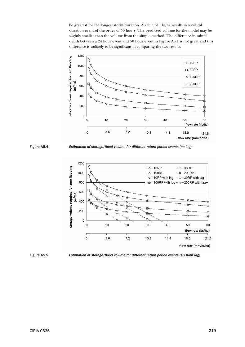
be greatest for the longest storm duration. A value of 1 l/s/ha results in a critical

duration event of the order of 50 hours. The predicted volume for the model may be

slightly smaller than the volume from the simple method. The difference in rainfall

depth between a 24 hour event and 50 hour event in Figure A5.1 is not great and this

difference is unlikely to be significant in comparing the two results.

Figure A5.4 Estimation of storage/flood volume for different return period events (no lag)

Figure A5.5 Estimation of storage/flood volume for different return period events (six hour lag)

CIRIA C635 219

Figure A5.6 Flood volume for different levels of storage provision for 10 year return period events (no lag)



CIRIA C635220


Figure A5.10 Flood volume for different levels of storage provision for 10 year return period events(six hour lag)


CIRIA C635 221



Figure A5.14 Flood flow rate for different levels of storage provision for 10 year return period events (no lag)

CIRIA C635222




CIRIA C635 223

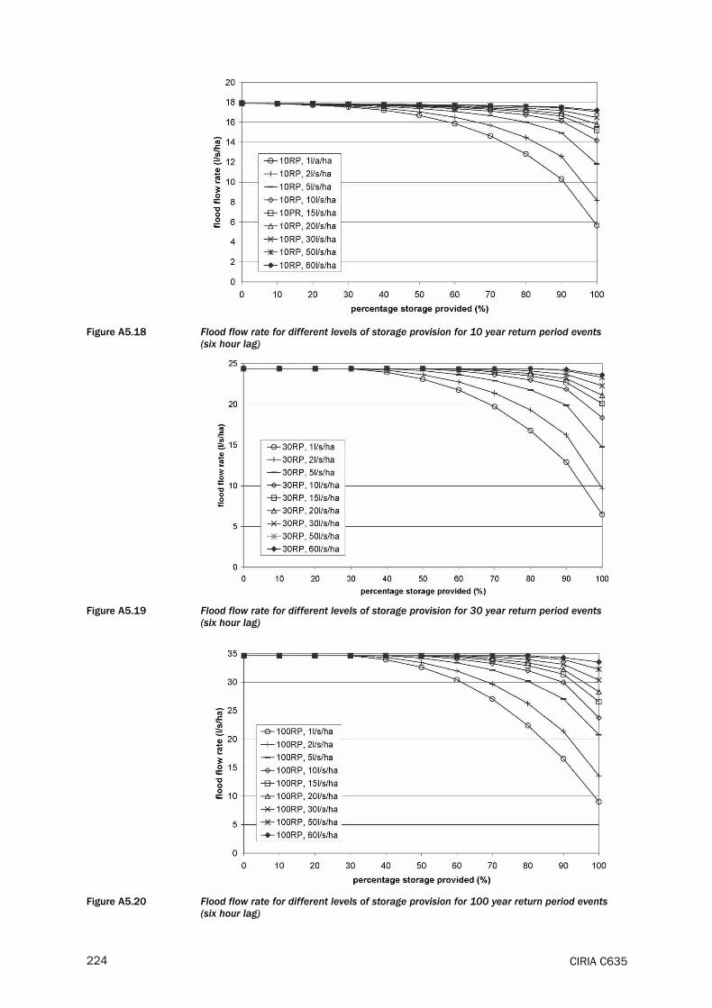
Figure A5.18 Flood flow rate for different levels of storage provision for 10 year return period events(six hour lag)



CIRIA C635224


CIRIA C635 225

A6 Design example of a permeable

pavement

Design example for a car park in the north with a one in 200 year return period design

storm. Determine the peak exceedance overflow rate and volume.

Table A6.1 Example of design data

Convert infiltration rate to a flow rate:

Permeable pavement also drains the impermeable surface area. For every 1 ha of

permeable surface there is 2 ha of impermeable surface.

Use Figure 9.12 to determine peak exceedance flow rate from the permeable

pavement.

Peak flow rate is 77 l/s/ha for a 200 year event with surface area ratio of two.

Exceedance volume for the pervious pavement system can be calculated using Figure

9.14. An infiltration rate of 3.3 l/s/per hectare of pavement and an area ratio of 2.0,

produces an exceedance volume of 1750 m³/ha.

Calculate exceedance overflow rate and volume for the car park which is 0.85 ha in

size.

Exceedance flow rate = 77 × 0.85 = 65.45 l/s

Exceedance volume = 1750 × 0.85 = 1488 m³

CIRIA C635226

Impermeable area = 1.7 ha

Pervious pavement area = 0.85 ha

Infiltration rate = 1.2 mm/hr

CIRIA C635 227

Figure A6.1 Flood flow rate from pervious pavement system – north (developed from Table 9.2)

Figure A6.2 Flood volume from pervious pavement system – north (developed from Table 9.4)

A7 Methods of estimating rural runoff

A7.1 The Rational Method

The Rational Method has its origins in the mid-19th century with Mulvaney in Ireland

and since its application to the design of sewers in England in the beginning of the 20th

century, this method has also become known as the Lloyds-Davies Equation. Due to its

simplicity, this method is still widely used in the design of small storm sewer systems but

can also be applied to the modelling of pervious catchments. The method predicts the

design peak runoff rate using the following formula in metric units:

(A7.1)

where:

Q = design peak runoff (in m³/s)

C = runoff coefficient

i = rainfall intensity for the design return period (in mm/hr) for a

specific duration related to the “time of concentration” of the

catchment

A = catchment area (in km²)

The estimate of the time of concentration can be made by a number of methods

(Kirpich, Bransby-Williams) which use catchment slope, area and length as parameters.

The Kirpich formula (1940) is:

TC = 0.063 (L/S 0.5) 0.8

where:

L = length (km)

The Rational Method is recognised as oversimplifying the rainfall runoff process but is

considered sufficiently accurate for runoff estimation for small contributing areas. The

main assumptions for the method are:

� rainfall occurs at uniform intensity for a duration at least equal to the time of

concentration of the catchment

� rainfall occurs uniformly over the entire area of the catchment

� the rainfall return period is the same as the runoff return period

� the factor C incorporates both the percentage runoff factor, an element for

attenuation and also accounts for the routing effect.

Refinements to the Rational Method (the Modified Rational Method of the Wallingford

Procedure) have been made to improve the accuracy of results through the split of the

runoff coefficient C into two coefficients; a routing and a volumetric coefficient. The

product of Cv and Cr for urban drainage is suggested as 0.6 and 1.3 respectively, this

value approximates close to one. However in a rural context Cv (percentage runoff)

would range from 0.1 through to 0.5 or so.

CIRIA C635228

Due to the difficulties of estimating the percentage runoff and the time of concentration,

the Rational Method is rarely used for estimating rural catchment peak flows.

A7.2 The TRRL method (Young and Prudhoe, 1973)

This method was developed specifically for small natural catchments to allow the

estimation of peak flows for the sizing of road culverts. It was developed from rainfall

and runoff data over several years of monitoring. The method used data collected from

four catchments plus one other catchment from a previous study. The TRRL method

was published before the Flood Studies Report (IOH, 1975) and provides a procedure for

the determination of peak flood flows for any return period from natural catchments

using key catchment parameters. The method resembles a “rational” type formula. The

following two equations define the time of concentration and the resulting peak flow

rate:

where:

TC = the time of concentration when all the catchment area is contributing

to the flood flow (hr)

LC = the catchment dimension, measured from outfall to upstream divide

(km)

N = dimensionless slope number equal to the ratio L/Z, where Z is the

rise from the outfall to the average height of the upstream divide

From this value for T, the peak flow Qc can be predicted using the following formula:

where:

A = catchment area (km³)

FA = dimensionless annual rainfall factor (=0.00127 RA – 0.321), and RA is

the average annual rainfall (mm)

RB = expected rainfall depth, which is given in tabulated form in Young

and Prudhoe (1973) based on values from the Bilham formula (mm).

The value for RB can be derived as follows for any value of T and

return period: 10/Return Period = 1.25 T(0.0394RB + 0.1)-3.55

This procedure is only considered suitable for natural catchments with an underlying

soil type of clay as this was the predominant nature of the catchments that were

measured. The authors state that the method is also applicable to catchments having

shallow soil overlying rock. It is generally recognised that the limited number of

catchments and period of measurement makes the equations application of limited

value. However for small catchments of with these type of soil characteristics, it is a

useful tool with which to carry out a check on the results produced by other methods.

CIRIA C635 229

A7.3 Flood Studies Report (FSR) (IOH, 1975)

The Flood Studies Report provides a number of different ways of predicting flows and

volumes for a given return period event. For the application to flood estimation from

ungauged natural catchments the most applicable procedure is the statistical approach

based on catchment descriptors.

The characteristic discharge adopted is the mean annual flood. This is defined as

QBAR and is given by:

where:

QBAR = mean annual flood (m³/s)

AREA = catchment area (km²)

STMFRQ = stream frequency in terms of the average number of stream

junctions per km²

S1085 = representative channel slope (in m/km) defined by points 10

per cent and 85 per cent upstream from the outflow point

from the catchment

SOIL = index determined from five soil types defined by the winter

rainfall acceptance potential (WRAP) map, RSMD is the net

one day five year rainfall minus the Soil Moisture Deficit

(mm)

LAKE = index of lake area as proportion of total area

Once the value of QBAR has been determined, design flood values for other return

periods are obtained using an appropriate regional growth curve. Growth curves have

been determined for the different areas of the United Kingdom and are contained

within the FSR. The growth curves were revised in FSSR 16 and are shown in figure

G1 as is the map of the hydrological regions for UK (Figure A7.2).

For completeness the WRAP map of UK is included in Figure A7.3 to provide an

indication of soil type across the country.

CIRIA C635230

Figure A7.1 Growth curve factors for UK hydrological regions (courtesy Institute of Hydrology 1983)

Figure A7.2 The growth curve regions of UK (courtesy Natural Environment Research Council 1975)

CIRIA C635 231

Figure A7.3 WRAP map of SOIL type for UK (courtesy Standing Technical Committee on Sewers andWater Mains, 1981)

A7.4 FSSR 6 Flood prediction for small catchments

Following on from the Flood Studies Report in 1975, a number of other mini studies were

carried out which refined various elements of the report. FSSR 6 was issued in 1978 to

try and provide a better prediction of runoff estimation for small catchments although

it was still limited to a minimum size of 50 ha, but less than 20 km³.

The mean annual flood was derived for new three and four parameter equations.

These are:

QBAR = 0.00066 AREA0.92 SAAR1.22 SOIL2.0

and:

QBAR = 0.0288 AREA0.90 RSMD1.23 SOIL2.0 STMFRQ0.23

Although they have the advantage of fewer parameters, particularly the three

parameter equation, where parameters can be very easily found, in practice it was

established that the accuracy of the predictions was not significantly improved from the

general six parameter equation for all catchments.

CIRIA C635232

The prediction of peak flows for small catchments was again revisited in the early 1990s

and is detailed in IOH Report 124 in Section A7.8.

A7.5 Poots and Cochrane method, 1979

A similar equation to FSSR 6 was derived by Poots and Cochrane from FSR data.

QBAR = 0.0136 AREA0.866 RSMD1.413 SOIL1.521

It is thought to provide similar levels of accuracy to FSSR 6.

A7.6 The ADAS method (Agricultural Development and

Advisory Service, 1980)

The ADAS report was produced primarily for agricultural drainage and is aimed at

providing information for the sizing of pipes for field drainage systems. The method is

based on measurements taken on a number of very small, rural areas measuring flows

collected by field drains. There are two forms of the ADAS method:

� basic method (which was derived for entirely clay type catchments)

� modified method (which was developed to take account of soil type and was based

on work from the Flood Studies Report (IOH, 1975) and the Soil Survey (1978).

The description below refers to the modified method in numerical form, (a graphical

procedure is also available). This method takes into account the design storm rainfall

and time of concentration for the required return period by using the Bilham formula.

The equation to estimate runoff from a site is of the form:

where:

Q = peak flow in l/s

Sm = soil type factor

A = catchment area in ha

FA = annual rainfall factor (note that FA is the same factor used in the

TRRL method in LR565) where:

FA = 0.00127 RA - 0.321

RA = average annual rainfall in mm

RB = rainfall depth (as defined by the Bilham formula)

TC = time of concentration (as defined in LR565)

Sm = soil index, which is based on five soil classes that are dependent on

their winter rainfall acceptance potential, and is defined as:

Sm=

S1, 2….denote the proportions of catchment covered by each of the

soil classes 1 to 5 and Su is the unclassified area of the catchment

covered by water or pavement. Tables for the determination of the

soil types are given in ADAS (1980). Soil class 1 has a low runoff

potential and soil class 5 has a high runoff potential. The parameter

Sm for a natural earth catchment can vary between 0.10 (very low

runoff) to 0.53 (very high runoff).

CIRIA C635 233

(0.10S1 + 0.30S2 + 0.37S3 + 0.47S4 = 0.53S5)

(1 – Su)

The predicted peak flow rate resulting from the ADAS equation should be taken as the

one year peak flood for the catchment. Flow rates for higher return periods can be

calculated using the appropriate regional growth curve in the Flood Studies Report. Care

should be taken in using the curves shown in the graphical method as they represent

the one, five and 10 year return periods.

The ADAS procedure is relatively simple to apply but a limitation of the procedure is

that the method should not be applied to catchments larger than 30 ha (or 0.3 km²).

Also, it should be recognised that it represents the measured soil inter-flow collected by

field drainage and so does not incorporate any over-land flow. The general consensus is

that it probably underestimates stream runoff for flows in streams for extreme events.

A7.7 The SCS method (Soil Conservation Service, 1985–1993)

A number of different procedures for applying the SCS method exist. The simplest case,

the TR-55 graphical method, is described here. In this method the peak discharge is

determined based on catchment characteristics (time of concentration, drainage area, curve

number) and a 24 hour rainfall amount and distribution. The method applies where:

� the catchment is accurately represented by a single curve number

� time of concentration is from 0.1 to 10 hours

� the catchment has only one main watercourse

� no valley or reservoir routing is required.

The curve number is a land use coefficient that dictates the relationship between total

rainfall depth and direct storm runoff. The time of concentration and travel time can

be computed to include sheet flow, shallow flow and channel flow. The method adjusts

the catchment response as the amount of rainfall increases, to take account of greater

saturation of the soil.

The SCS method is widely used in the United States for estimating peak runoff rates on

small drainage basins. Application of the method is simple and direct; however,

variation in results occurs in practice due to the choice of procedure to determine the

time of concentration and to choose the curve number. The TR-55 procedure is

suggested for drainage areas up to 50 km².

As is apparent from the above, a limitation of the SCS procedure for UK applications is

that all the data used to generate the curve number parameter is from the United

States. Equivalent rainfall types and other terms are required in order to apply this

method to the UK.

A7.8 Institute of Hydrology Report 124 (1994)

The Institute of Hydrology Report 124 was published in 1994 and describes research

for flood estimation in small catchments. The research was based on 71 small rural

catchments. An adjusted regression equation was produced to calculate the mean

annual flood for small rural catchments. This methodology should preferably only be

applied to a catchment drained by a well-defined watercourse and where the

catchments are larger than 50 ha (ie 0.5 km²). This is the latest and the current most

accepted method for predicting runoff. However as there is no slope function, in some

instances it is still worthwhile checking the result obtained against one or more of the

other methods.

CIRIA C635234

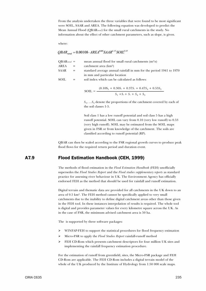
From the analysis undertaken the three variables that were found to be most significant

were SOIL, SAAR and AREA. The following equation was developed to predict the

Mean Annual Flood (QBARrural) for the small rural catchments in the study. No

information about the effect of other catchment parameters, such as slope, is given.

where:

QBARrural = mean annual flood for small rural catchments (m³/s)

AREA = catchment area (km²)

SAAR = standard average annual rainfall in mm for the period 1941 to 1970

in mm and particular location

SOIL = soil index which can be calculated as follows:

S1, …S5 denote the proportions of the catchment covered by each of

the soil classes 1-5.

Soil class 1 has a low runoff potential and soil class 5 has a high

runoff potential. SOIL can vary from 0.10 (very low runoff) to 0.53

(very high runoff). SOIL may be estimated from the SOIL maps

given in FSR or from knowledge of the catchment. The soils are

classified according to runoff potential (RP).

QBAR can then be scaled according to the FSR regional growth curves to produce peak

flood flows for the required return period and duration event.

A7.9 Flood Estimation Handbook (CEH, 1999)

The methods of flood estimation in the Flood Estimation Handbook (FEH) unofficially

supersedes the Flood Studies Report and the Flood studies supplementary reports as standard

practice for assessing river behaviour in UK. The Environment Agency has officially

endorsed FEH as the method that should be used for rainfall and runoff estimation.

Digital terrain and thematic data are provided for all catchments in the UK down to an

area of 0.5 km². The FEH method cannot be specifically applied to very small

catchments due to the inability to define digital catchment areas other than those given

in the FEH tool. In these instances interpolation of results is required. The whole tool

is digital and provides parameter values for every kilometre square across the UK. As

in the case of FSR, the minimum advised catchment area is 50 ha.

The is supported by three software packages:

� WINFAP-FEH to support the statistical procedures for flood frequency estimation

� Micro-FSR to apply the Flood Studies Report rainfall-runoff method

� FEH CD-Rom which presents catchment descriptors for four million UK sites and

implementing the rainfall frequency estimation procedure.

For the estimation of runoff from greenfield, sites, the Micro-FSR package and FEH

CD-Rom are applicable. The FEH CD-Rom includes a digital terrain model of the

whole of the UK produced by the Institute of Hydrology from 1:50 000 scale maps.

CIRIA C635 235

SOIL =(0.10S1 + 0.30S² + 0.37S³ + 0.47S4 + 0.53S5

S1 +S² + S³ + S4 + S5

The CD-Rom allows the delineation of catchment boundaries to be carried out

automatically. The catchment boundaries based on the terrain map are inevitably

approximate. However, it should be noted that discrepancies are most likely to arise in

small catchments.

The general philosophy behind flood frequency estimation in the FEH is as follows:

� flood frequency is best estimated from gauged data

� where gauged data are not available, data transfers from nearby or similar

catchments are useful

� estimation of floods from catchment descriptors alone should be used as a method

of last resort.

It should be noted that the FEH provides catchment descriptors for all sites draining

an area of 0.5 km² (50 ha) or greater based on a 50 m resolution DTM model. The

lower limit reflects that:

� very small catchments are poorly represented in the data sets used to calibrate the

models for estimating flood frequency from catchment descriptors

� digital terrain and thematic data may not be well resolved on very small

catchments.

The statistical procedures and rainfall-runoff methods used in the FEH are outlined below.

A7.10 Statistical procedures for flood estimation

The major changes to the statistical procedures for flood frequency estimation

compared with the Flood Studies Report are as follows:

� the median annual flood QMED rather than QBAR is used as the index variable

� where no gauged data are available, QMED is estimated from catchment descriptors

based on digital data rather than derived manually from maps

� the derivation of the growth curve for the catchment is flexible rather than fixed

and is generally based on pooling of relevant flood peak data, or in a few cases, the

catchment descriptors

� catchment similarity is initially judged in terms of size, wetness and soil.

The index flood represents the typical magnitude of a flood expected at a given site.

The FEH uses the median annual flood QMED as the index flood. QMED is the median

value of the annual maximum flow series. There are several methods for estimating

QMED. These are described below.

If the catchment is gauged then QMED can be estimated from the annual maximum flow

data. This method is recommended if there are 14 or more years of records. Where

there are more than two years and less than 14 years of annual maximum flows, the

peaks over threshold data should be used.

The recommended procedure for QMED at sites where there are no flood peak data is to

transfer data from a nearby donor site or from a more distant analogue catchment. A

prerequisite for the data transfer is that the donor/analogous catchment is

hydrologically similar to the catchment of interest. Further details of these data transfer

techniques are given in the FEH.

CIRIA C635236

For ungauged rural catchments where data transfer is not possible, QMEDrural can be

estimated from five catchment descriptors. These are:

� drainage area (AREA)

� average annual rainfall (SAAR)

� soil drainage type represented by SPRHOST and BFIHOST

� storage attenuation due to reservoirs and lakes (FARL)

� baseflow index (BFI).

FEH catchment descriptors are based on drainage boundaries defined by a digital

terrain model. Inconsistencies may arise on small catchments, this method should only

be used as a last resort in this situation.

A7.11 Rainfall – runoff method for flood estimation

The rainfall-runoff method remains similar to that described in the Flood Studies Report.

However, where no gauged data are available, catchment descriptors should be based

on the FEH digital data, rather than derived manually from maps. The unit

hydrograph method used by the Micro-FSR software package is still applicable.

The FEH rainfall analysis was carried out for the period 1971 to 1990 whereas the FSR

analysis was based on data between 1941 and 1970. The results show quite significant

differences when compared with the FSR rainfall characteristics. Although there may be

an element of climate change, the view is generally held that the difference is more a

function of the statistical methods used for analysing the data. These differences can be

as high as 40 per cent in parts of the south east of the UK, while other areas have very

similar predicted depths. The difference between FSR and FEH for more extreme

rainfall nearly always show a greater rainfall in the FEH assessment of rainfall depth.

The main exceptions are in east Scotland and Northern Ireland where FSR tends to

predict higher rainfall depths. For small return periods the difference between FSR

and FEH is generally less though there are hot-spots, such as the Reading area, which

still has a significant increase in rainfall depth for any return period. Figure A7.4

illustrates the differences in rainfall depths between FSR and FEH across the UK.

CIRIA C635 237

Figure A7.4 FSR/FEH rainfall depth ratios for the one hour 25 year event (courtesy UKWIR)

Estimation of QMED (median annual maximum flood) from catchment descriptors is

produced using the following equation:

where:

FARL = factor to account for the presence of reservoirs and lakes

SPRHOST = soil parameters

RESHOST = soil parameters

AE = area exponent the other factors are defined by FSR

FEH uses a 29-class Hydrology of Soil Types (HOST) classification and the database

gives the percentage of each class present in a 1 km × 1 km grid. Currently there is no

paper map version of the country showing the HOST soil classes.

Rainfall growth factors in FSR were considered to be over general, masking local and

regional variations in rainfall. The FEH procedure takes more account of local data,

both in constructing the focused growth curves and in mapping the standardising

variable, RMED.

The following advice is given in the FEH manual as to the applicability of QMED

(median annual maximum flood) from catchment descriptors:

CIRIA C635238

� the model is only applicable to rural UK catchments

� the model should not be applied to unusual catchments

� the model should not be relied on if the runoff is strongly influenced by lakes and

reservoirs

� QMED is likely to be less accurately estimated for permeable catchments.

A7.12 Advantages and disadvantages of the Flood Estimation

Handbook techniques

The advantages of the Flood Estimation Handbook are as follows:

� uses pooling and transfer of flow data to estimate flows from ungauged catchments

� the catchment area and descriptors are calculated digitally from a digital terrain

model

� the pooling of the flood flow data for defining the growth curve is flexible and

tailored to fit the subject site.

The disadvantages of the Flood Estimation Handbook are as follows:

� requires detailed hydrological knowledge to apply the techniques correctly

� requires access to and detailed knowledge of the use of the FEH CD-Rom and

WINFAP_FEH software

� catchments below 0.5 km² cannot be defined on the Flood Estimation Handbook

digital terrain model

� definition of small catchments (ie catchments with an area less than 1 km²) may be

inaccurate in some cases particularly adjacent to urban areas where contours are

not well defined

� small, partially urbanised catchments, where the urban fraction is significant,

should not use the catchment descriptor method.

A7.13 FSR, and FSSR 5, 6 and 16 percentage runoff estimation

The original FSR produced a formula for predicting the volume of runoff from a

catchment. The correlation coefficient R² was quite low at 0.43. The formula was

revisited in FSSR 5 (1979) Design flood estimation in catchments subject to urbanisation and

also in FSSR 6 (1978) Flood prediction for small catchments and finally in FSSR 16 (1985)

The FSR rainfall – runoff model parameter estimation equations updated. Percentage runoff

was not addressed again in IOH Report 124.

In general, the formula are all of the same form using SOIL, a function of CWI and

SAAR and rainfall depth. There is also a final term for the additional runoff which

would take place from any urban areas within the catchment. None of the models

included a slope term. The SOIL term is a weighted SOIL value based on the amount

of area of each soil type in the catchment. As FSSR 16 was the final version this is the

only one reported here, and it is the presumed that it relates to flood response and

only relates to extreme events.

The FSSR 16 formula is:

PRRURAL = SPR + DPRCWI + DPRRAIN

CIRIA C635 239

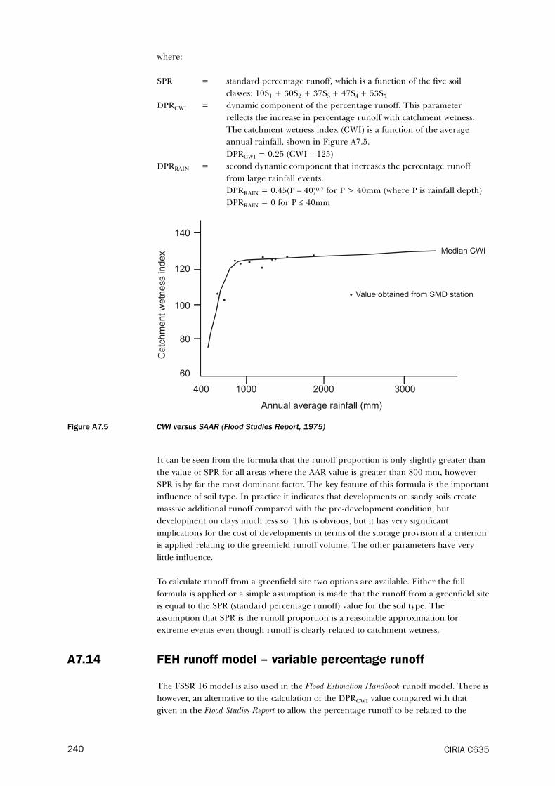
where:

SPR = standard percentage runoff, which is a function of the five soil

classes: 10S1 + 30S2 + 37S3 + 47S4 + 53S5

DPRCWI = dynamic component of the percentage runoff. This parameter

reflects the increase in percentage runoff with catchment wetness.

The catchment wetness index (CWI) is a function of the average

annual rainfall, shown in Figure A7.5.

DPRCWI = 0.25 (CWI – 125)

DPRRAIN = second dynamic component that increases the percentage runoff

from large rainfall events.

DPRRAIN = 0.45(P – 40)0.7 for P > 40mm (where P is rainfall depth)

DPRRAIN = 0 for P ≤ 40mm

Figure A7.5 CWI versus SAAR (Flood Studies Report, 1975)

It can be seen from the formula that the runoff proportion is only slightly greater than

the value of SPR for all areas where the AAR value is greater than 800 mm, however

SPR is by far the most dominant factor. The key feature of this formula is the important

influence of soil type. In practice it indicates that developments on sandy soils create

massive additional runoff compared with the pre-development condition, but

development on clays much less so. This is obvious, but it has very significant

implications for the cost of developments in terms of the storage provision if a criterion

is applied relating to the greenfield runoff volume. The other parameters have very

little influence.

To calculate runoff from a greenfield site two options are available. Either the full

formula is applied or a simple assumption is made that the runoff from a greenfield site

is equal to the SPR (standard percentage runoff) value for the soil type. The

assumption that SPR is the runoff proportion is a reasonable approximation for

extreme events even though runoff is clearly related to catchment wetness.

A7.14 FEH runoff model – variable percentage runoff

The FSSR 16 model is also used in the Flood Estimation Handbook runoff model. There is

however, an alternative to the calculation of the DPRCWI value compared with that

given in the Flood Studies Report to allow the percentage runoff to be related to the

CIRIA C635240

increasing catchment wetness through an event. Instead of CWI factor being a constant

related to SAAR, it is a function of the API5 and SMD and is given by the following

equation:

CWI = 125 + API5 – SMD

where:

API5 = five day antecedent moisture precipitation index

SMD = pre-event soil moisture deficit

SMD values are a function of the soil type, antecedent rainfall and evaporation. In

winter months and in very wet conditions, SMD will usually be close to zero, which

represents saturation of the soil field capacity. SMD values of 100 mm or more can

occur in summer.

This equation allows the prediction of greenfield runoff of an event including those

which are not extreme (that would not cause river flooding). This has considerable

advantages in that runoff from a catchment can be assessed for all events for a site. This

means that the design of drainage systems can assessed against a prediction of the

greenfield runoff for a range of rainfall and runoff criteria.

CIRIA C635 241

References

ADAS (1980)

“The ADAS Method”

In: The design of field drainage pipe systems A D Bailey, C W Dennis, G L Harris and

Horner. MAFF 5, Land Drainage Service, Research and Development, December 1982

ALLITT, M (2004)

“Using DTMs to determine locations of permeable runoff into sewerage networks”

In: WaPUG Scottish Meeting 2004, Richard Allitt Associates Ltd, West Sussex

ALLITT, R C (1997)

Overland flood routing

WaPUG Usernote 37, WaPUG, Richard Allitt Associates Ltd, West Sussex

ASHLEY, R M, ENGLAND, K, DAVIE, J and ABBOT, A (2005)

Review to consider the future water management and the associated problems of flooding in the

Bradford district

Policy Development Service, City of Bradford Metropolitan District Council

Department of Policy and Performance, Bradford. Go to:

<www.bradford.gov.uk/NR/rdonlyres/AB1C2216-0062-49FD-BF3B-

3A525B9E606E/0/Final_Review_WM.pdf>

AUCKLAND REGIONAL COUNCIL (2003)

Stormwater management devices: design guide

2nd edition, TP10, Auckland Regional Council, New Zealand. Go to:

<www.arc.govt.nz/environment/water/stormwater/stormwater-management-

devices.cfm>

BOONYA-AROONNET, S, WEESAKUL, S and MARK, O (2002)

“Modelling of urban flooding in Bangkok”

In: Proc 9th Int Conf on Urban Drainage (9ICUD), Global Solutions for Urban Drainage

Orlando, USA

BRE (2000)

Good building guide 38: Disposing of rainwater

GG28, Building Research Establishment, Garston (ISBN: 978-1-84806-205-4)

CEH (1999)


Centre for Ecology and Hydrology, UK (ISBN: 978-1-90669-800-3)

CHOW, V T (1959)

Open-channel hydraulics

McGraw-Hill Kogakusha Ltd, Japan (ISBN: 978-0-07010-776-2)

CIRIA (2003a)

Improving the flood resistance of your home – Advice sheet 6: Flood-resistant floors

CIRIA, London. Go to: <www.ciria.org.uk/flooding/pdf/CIRIA_Advice_sheet_6.pdf>

CIRIA C635242

CIRIA (2003b)

Improving the flood resistance of your home – Advice sheet 7: Flood-resilient services

CIRIA, London. Go to: <www.ciria.org.uk/flooding/pdf/CIRIA_Advice_sheet_7.pdf>

CLAUSEN, L and CLARK, P B (1990)

“The development of criteria for predicting dambreak flood damages using modelling

of historical dam failures”

In: Proc Int Conf on River Flood Hydraulics, W R White (ed), John Wiley, and Hydraulic

Research Ltd, Chichester, pp 369–380

CLG (2000)

Planning Policy Guidance (PPG) 3: Housing

Communities and Local Government, London (ISBN: 978-0-11753-976-7)

CLG (2001)

Planning Policy Guidance (PPG) 25: Development and flood risk

Communities and Local Government, London

CLG (2003)

Preparing for floods: interim guidance for improving the flood resistance of domestic and small

business properties

01CD1025, Communities and Local Government, London

CLG (2004)

Planning Policy Guidance (PPG) 12: Local development frameworks

Communities and Local Government, London (ISBN: 978-0-11753-926-6)

DEFRA (2004)

Making space for water. Developing a new Government strategy for flood and coastal erosion risk

management in England. A consultation exercise

Department for Environment, Food and Rural Affairs, London. Go to:

<www.floodprotectionassoc.co.uk/cms/documents_library/consultation.pdf>

DEPARTMENT OF THE ENVIRONMENT (2006)

Planning Policy Statement (PPS) 15: Planning and flood risk

Planning Department, Department of the Environment, Belfast

ELLIOTT, C R N and LEGGETT, D J (2002)

Reducing the impacts of flooding – extemporary measures

Funders Report IP/45, CIRIA, London. Go to:

<www.ciria.org.uk/flooding/pdf/flooding.pdf>

ESCARAMEIA, M and MAY, R W P (1996)

Surface water channels and outfalls: recommendations on design

SR406, HR Wallingford, UK

ESCARAMEIA, M, GASOWSKI, Y and MAY, R (2002)

“Grassed drainage channels – hydraulic resistance characteristics”

In: Proc the ICE – Water and Maritime Engineering, Vol 154, No 4, pp 333–341

EVANS, E, ASHLEY, R, HALL, J, PENNING-ROWSELL, E, SAYERS, P, THORNE, C,

and WATKINSON, A (2004)

Future flooding scientific summary: Volume II – managing future risks

Office of Science and Technology, London

CIRIA C635 243

GARVIN, S, REID, J and SCOTT, M (2005)

Standards for the repair of buildings following flooding

C623, CIRIA, London (ISBN: 978-0-86017-623-7). Go to: <www.ciria.org>

HALL, M J, HOCKIN, D L, and ELLIS, J B (1996)

Design of flood storage reservoirs

B14, CIRIA, London (ISBN: 978-0-86017-393-9). Go to: <www.ciria.org>

HELSINKI UNIVERSITY OF TECHNOLOGY (2001)

Development of rescue actions based on dam break analysis. Appendix 2: The use of physical

models in dam-break flood analysis

Finnish Environment Institute, Helsinki. Go to:

<http://ec.europa.eu/echo/civil_protection/civil/pdfdocs/rescdam_rapportfin.pdf>

HIGHWAYS AGENCY (2000)

Volume 4 Geotechnics and Drainage, Section 2 Drainage, Part 3, HA 102/00: Spacing of Road

Gullies

Design Manual for Roads and Bridges, The Stationary Office, Norwich. Go to:

<www.dft.gov.uk/ha/standards/dmrb/>

HR WALLINGFORD, FLOOD HAZARD RESEARCH CENTRE, MIDDLESEX

UNIVERSITY AND RISK AND POLICY ANALYSTS LTD (2004)

R&D outputs: flood risk to people phase 2

FD2321/IR2, Defra/Environment Agency, Flood and Coastal Defence R&D Programme

ICE (2001)

Learning to live with rivers. Final report of the Institution of Civil Engineers Presidential

Commission to review the technical aspects of flood risk management in England and Wales

Institution of Civil Engineers, London (ISBN: 0-7277310-4)

IOH (1975)

Flood Studies Report

Institute of Hydrology, Wallingford, UK

IOH (1983)

Flood studies supplementary report No. 14 regional growth curves reviewed


KELLAGHER, R (2004)

Drainage of development sites – a guide

X108, CIRIA, London (ISBN: 978-0-86017-900-9). Go to: <www.ciria.org>

LANCASTER, J W, PREENE, M and MARSHALL, C T (2004)

Development and flood risk – guidance for the construction industry


MARSHALL, D C W and BAYLISS, A C (1994)

Report 124 Flood estimation for small catchments


MARTIN, P, TURNER, B, WADDINGTON, K, DELL, J, PRATT, C, CAMPBELL, N,

PAYNE, J and REED, B (2000a)

Sustainable urban drainage systems: design manual for Scotland and Northern Ireland


CIRIA C635244

MARTIN, P, TURNER, B, WADDINGTON, K, DELL, J, PRATT, C, CAMPBELL, N,

PAYNE, J and REED, B (2000b)

Sustainable urban drainage systems: design manual for England and Wales


MARTIN, P, TURNER, B, DELL, J, PAYNE, J, ELLIOTT, C and REED, B (2001)

Sustainable urban drainage systems: best practice manual for England, Scotland, Wales and

Northern Ireland

C523, CIRIA, London (ISBN: 978-0-86017-523-0). <www.ciria.org>

MURPHY, D (2003)

Environment Agency Strategy for Flood Risk Management (2003/4–2007/8), Version 1.2

Environment Agency, Bristol. Go to:

<www.jubileeriver.co.uk/frm_strategy_v1.2_573731.pdf>

NANIA, L, GOMEZ, M and DOLZ, J (1999)

“Numerical and experimental study of the urban storm runoff in a street network”

In: Proc of 8th Int Conf on Urban Storm drainage, Sydney, Australia, pp 849–856

NANIA, L, GOMEZ, M and DOLZ, J (2002)

“Analysis of risk associated to the urban runoff. Case study: City of Mendoza, Argentina”

In: Proc 9th Int Conf on Urban Drainage (9ICUD), Global Solutions for Urban Drainage

Orlando, USA

NATIONAL ASSEMBLY FOR WALES (2004)

Technical advice note (Wales) 15: Development and flood risk

National Assembly for Wales, Cardiff

NERC (1978)

Flood prediction for small catchments

Flood Studies Supplementary Report No. 6, Natural Environmental Research Council,

Swindon

NERC (1985)

The FSR rainfall-runoff model parameter estimation equations updated

Flood Studies Supplementary Report No. 16, Natural Environmental Research

Council, Swindon

NORTH EAST FLOODING ADVISORY GROUP (2002)

Drainage impact assessment. Guidance for developers and regulators

DP 30 3/02, North of Scotland Water Authority, Scottish Environment Protection

Agency, Aberdeenshire Council and and Aberdeen City Council, Scotland. Go to:

<www.aberdeenshire.gov.uk/flooding/report/sepa_dia.pdf>

NSWG (2004)

Interim code of practice for sustainable urban drainage systems

National SuDS Working Group, CIRIA, London. Go to:

<www.ciria.org.uk/suds/icop.htm>

O’LEARY, J (2004)

Sorting out responsibilities for flooding at Titford road

WaPUG Training Day – solving flooding problems, Midlands Engineering Centre,

Birmingham

CIRIA C635 245

OFWAT (2002)

Flooding from sewers – a way forward. Consultation

Ofwat (The Water Services Regulation Authority) , Birmingham. Go to:

<www.ofwat.gov.uk/>

PENNING-ROWSELL, E, JOHNSON, C, TUNSTALL, S, TAPSELL, S, MORRIS, J,

CHATTERTON, J, COKER, A and GREEN, C (2003)

The benefits of flood and coastal defence: techniques and data for 2003

Flood Hazard Research Centre, Middlesex University

POOTS, A D and COCHRANE, S R (1979)

“Design flood estimation for bridges, culverts and channel improvement works on small

rural catchments”

In: ICE Proceedings, Volume 68, Issue 2, May 1980, Institution of Civil Engineers,

London, pp 317–322

RAMSBOTTOM, D, FLOYD, P and PENNING-ROWSELL, E (2003)

Flood risks to people Phase 1

R&D Technical Report FD2317, Defra/Environment Agency, Flood and Coastal Defence

R&D Programme

REGIONAL FLOOD CONTROL DISTRICT (1999)

Hydrologic criteria and drainage design manual

Regional Flood Control District, Clark County NV. Go to:

<www.ccrfcd.org/hcddm.htm>

REITER, P (2000)

“International methods of risk analysis, damage evaluation and social impact studies

concerning dam-break accidents”

In: Proc Int Seminar on the Rescdam Project, Seinäjoki 1–5 October 2000

SCOTTISH GOVERNMENT (2004)

Scottish Planning Policy SPP7 – planning and flooding

The Scottish Government, Edinburgh (ISBN: 0-7559-2439-8). Go to:

<http://home.scotland.gov.uk/home>

SCOTTISH GOVERNMENT (2004)

Planning advice note (PAN) 69 Planning and building standards advice on flooding

The Scottish Government, Edinburgh. Go to: <http://home.scotland.gov.uk/home>

SHAFFER, P, ELLIOTT, C, REED, J, HOLMES, J and WARD, M (2004a)

Model agreements for sustainable water management systems. Model agreements for SUDS


SHAFFER, P, ELLIOTT, C, REED, J, HOLMES, J and WARD, M (2004b)

Model agreements for sustainable water management systems. Model agreement for rainwater and

greywater use systems


SOIL CONSERVATION SERVICE (1985)

National engineering handbook series, Part 630 Hydrology, Chapter 4, Storm Rainfall Depth

Natural Resource Conservation Service, United States Department of Agriculture.

Go to: <www.mi.nrcs.usda.gov/technical/engineering/neh.html>

CIRIA C635246

STANDING TECHNICAL COMMITTEE ON SEWERS AND WATER MAINS (1981)

Design and analysis of urban storm drainage: the Wallingford Procedure

Department of the Environment, London (ISBN: 978-0-90109-027-0)

UKWIR (2004)

Climate change and the hydraulic design of sewerage systems. Volume I: Climate change effects on

rainfall, IC Seasonality study

Project: 03/CL/10/3, UK Water Industry Research (ISBN: 1-84057-328-7)

WALESH, S G (1999)

Street storage system for control of combined sewer surcharge – retrofitting stormwater storage into

combined sewer systems

Contract No. 8C-R416-NTSX, National Risk Management Research Laboratory, Office

of Research and Development, U.S. Environmental Protection Agency, Cinncinnati, OH

45268

WATER UK and WRc (2001)

Sewers for adoption 5th edition

WRc, Swindon

WILSON, S, BRAY, R and COOPER, P (2004)

Sustainable drainage systems. Hydraulic, structural and water quality advice


WISNER, P E, KASSEM, A M and CHEUNG, P W (1982)

“Analysis of dual drainage systems by OTTSWMM”

In: Proc: 1st Int Seminar on Urban Drainage Systems, Southampton, UK pp 2.93–2.101

WOODS-BALLARD, B, KELLAGHER, R, MARTIN, P, JEFFERIES, C, BRAY, R and

SHAFFER, P (2007)

The SuDs Manual


YOUNG, C P and PRUDHOE, J (1973)

The estimation of flood flows from natural catchments

TRRL Report LR 565, Transport Research Laboratory, Berkshire

CIRIA C635 247

Acts

Environment Act 1995 (c.25)

Land Drainage Act 1991 (c.59)

Land Drainage Act 1994 (c.25)

Highways Act 1980 (c.66)

Planning and Compensation Act 1991 (c.34)

Planning and Compulsory Purchase Act 2004 (c.4)

Reservoirs Act 1975 (c.23)

Water Act 1989 (c. 15)

Water Industry Act 1991 (c.56)

Water Industry Act 1999 (c. 9) Explanatory Notes

Water Resources Act 1991 (c.57)

Directives

Directive 2000/60/EC of the European Parliament and of the Council of 23 October 2000

establishing a framework for Community action in the field of water policy (the Water Framework

Directive)

Legal rulings

British Waterways Board v/s Severn Trent Water Plc, (Court of Appeal 2001)

Thames Water v/s Marcic Appeal ruling, (Court of Appeal 2002)

Regulations

HM GOVERNMENT (2000) The Building Regulations No. 2531:

� Approved Document C (2004) Site preparation and resistance to contaminants and

moisture

� Approved Document H (2002) Drainage and waste disposal

� Approved Document M (2004) Access to and use of buildings

Standards

BS EN 752-4:1998 Drain and sewer systems outside buildings – Part 4: Hydraulic design and

environmental considerations

BS EN 12056-3:2000 Gravity drainage systems inside buildings – Part 3: Roof drainage, layout

and calculation

BS EN 752-3:1997 Drain and sewer systems outside buildings – Part 3: Planning

BS EN 1253-1:2003 Gullies for buildings – Part 1: Requirements

CIRIA C635248

Glossary

Annual probability The estimated probability of a flood of given magnitude

occurring or being exceeded in any year. Expressed as,

for example, 1 in 100 chance or 1 per cent.

Attenuation A reduction of the rate of flow with a consequent

increase in the duration of the flow.

Catchment The area contributing flow or runoff to a point on a

drainage or river system. Can be divided into sub-

catchments.

Climate change Long term variations in global temperature and

weather patterns both natural and as a result of human

activity, primarily greenhouse gas emissions.

Conveyance The movement of water from one location to another.

Conveyance capacity The capacity of a system to convey flow. In piped

systems, the conveyance capacity will exceed the pipe

full capacity due to flow backing up in manholes.

Default pathways Surface flood pathways which have not been designed

to convey flows.

Depression storage The depth of water retained on the ground surface in

puddles or other depressions.

Design criteria A set of standards agreed by the developer, planners

and regulators that the proposed system should satisfy.

Design event A historic or notional flood event of a given annual

flood probability, against which the suitability of a

proposed development is assessed and mitigation

measures, if any, are designed.

Designed pathways Surface flood pathways which have been designed to

convey flows.

Detention basin A vegetated depression that is normally dry except

following storm events constructed to store water

temporarily to attenuate flows. May allow infiltration of

water to the ground.

Development The carrying out of building, engineering, mining or

other operations in, on, over or under land or the

making of any material change in the use of any

buildings or other land.

Discharge Rate of water flow.

Downstream system The system to which the defined area that is subject to

exceedance discharges to, eg an urban drainage system

or watercourse.

Evapo-transpiration The process by which the earth’s surface or soil loses

moisture by evaporation of water and its uptake and

then transpiration from plants.

CIRIA C635 249

Exceedance flood A study to assess the risk of a site or area being affected

by risk assessment exceedance flow, and to assess the effect that any

changes made to the areas or site will have on the

exceedance flood risk.

Exceedance flow Excess flow that appears on the surface once the

conveyance capacity of the minor system is exceeded.

Extreme events Rainfall events that are sufficient in size to produce

exceedance flows.

Fluvial flooding Flooding from a river or other watercourse.

Freeboard The difference between the level of where flooding or

overtopping may occur and the designed water level.

Greenfield runoff rate The rate of runoff that would occur from the site in its

undeveloped, and undisturbed, state.

Groundwater Water in the ground, usually referring to water in the

saturated zone below the water table.

Gully Opening in the road pavement that allows water to

enter conventional drainage systems, often covered by

a metal grate.

Hydrograph A graph, that shows the variation with time of the level

or discharge in a watercourse.

Hydraulic gradient In an open channel, the gradient of the water surface;

in a pressurised pipe, the gradient joining points to

which water would rise in pressure tappings.

Impermeable surface An artificial non-porous surface that generates a

surface water runoff following rainfall.

Infiltration The passage of water through a surface, either the

pervious surface or the underlying ground.

Infiltration system A system designed to aid infiltration of surface water to

the ground.

Internal drainage board Body with powers and duties relating to ordinary

watercourses within an internal drainage district.

Level of protection A target level in which no flooding should occur, eg a

0.02 probability of a property being flooded.

Level of service A level of water, usually specified as a return period to

which an urban drainage system is designed to provide

as a minimum, referred to as a target level.

Local planning authority Body responsible for planning and controlling

development, through the planning system.

Main river A watercourse designated on a statutory map of main

rivers, maintained by Defra.

Major system The system of above ground flood pathways, including

both open and culverted watercourses.

Minor system The formal or designed drainage system.

Ordinary watercourse A watercourse that is not a private drain and is not

designated a main river.

CIRIA C635250

Overland flow Overland flow is water flowing over the ground surface

that has not entered or has escaped from a natural

drainage channel or artificial drainage system (other

commonly used terms for this phenomenon are pluvial

flooding or surface water runoff flooding).

Percentage runoff The proportion of rainfall that runs off a surface.

Pervious surface A surface that allows inflow of rainwater into the

underlying construction or soil.

Pluvial flooding Flooding caused by overland flow that has not entered

into a natural drainage channel or artificial drainage

system.

Pond Permanently wet basin designed to retain stormwater.

Probability of The statistical probability of a hydrological event

exceedance (rainfall or flow) of a given magnitude being exceeded

in any individual year.

Public sewer A sewer that is vested and maintained by the sewerage

undertaker.

Return period The frequency that an event occurs. A one hundred

year storm is one that occurs on average once every

100 years, ie its annual probability of exceedance is 1

per cent (1/100).

Runoff The flow of water, caused by rainfall, from an area over

the ground surface to the drainage system. This occurs

if the ground is impermeable or is saturated.

Runoff co-efficient A measure of the amount of rainfall that is converted

to runoff.

Sacrificial areas Low value land to which exceedance flood volumes can

be discharged and retained for limited periods of time.

Sewer A pipe of channel with a proper outfall that takes

domestic foul and/or surface water form buildings and

associated paths and hardstandings from two or more

curtilages.

Sewerage undertaker An organisation with the legal duty to provide

sewerage services in an area, including the disposal of

surface water from roofs and yards of premises.

Sewers for adoption A guide agreed between sewerage undertakers and

developers (through the House Builders Federation)

specifying the standards to which private sewers need

to be constructed to facilitate adoption.

Soakaway A subsurface structure into which surface water is

conveyed to allow infiltration into the ground.

Stakeholders A single person or group of people, company or

organisation with an interest in managing exceedance.

Surface flood pathways Routes in which exceedance flows are conveyed on the

ground.

Sustainable Development that meets the needs of the present

development without compromising the ability of future generations

to meet their own needs.

CIRIA C635 251

252 CIRIA C635

Sustainable drainage A sequence of management practices and control

systems structures, often referred to as SuDS, designed to

drain surface water in a more sustainable manner than

some conventional techniques. Typically, these

techniques are used to attenuate rates of runoff from

development sites. Sometimes called sustainable urban

drainage systems.

Swale A shallow vegetated channel designed to conduct and

retain water, but may also permit infiltration.

Target level A defined level of protection that is satisfied when

failure occurs less frequently than the specified level.

Time of entry Time taken for rainwater to reach an inlet into the

drainage system after hitting the ground.

Trigger level When failure occurs more frequently than the

identified level of protection.

Watercourse Any natural or artificial channel that conveys surface

and/or groundwater.

Abbreviations

á Proportion of paved area draining to the network or

directly to the river

â Proportion of pervious area draining to the network or

directly to the river

A Catchment area

AC Cross-sectional area of flow

AE Area exponent

Ae / Ai (ch9) Equivalent Impermeable Area

AF Cross-sectional area of flow in channel

ADAS Agricultural drainage advisory service

API5 Five day antecedent precipitation index

AREA Catchment area

ARF Areal reduction factor

b Average width at entry to downstream channel

BFI Baseflow index

BFIHOST Soil parameters

C Runoff co-efficient

CP Decay constant

CEH Centre for Ecology and Hydrology

CFD Computational fluid dynamics

CWI Catchment wetness index

D Depth

dc Critical depth

Defra Department of Environment Food and Rural Affairs

DoE(NI) Department of Environment (Northern Ireland)

DPR Dynamic component of the percentage runoff

DTLR Department of Transport, Local Government and the

Regions

DTM Digital terrain model

EA Environment Agency

EFRA Exceedance flood risk assessment

FA Annual rainfall factor

FARL Factor to account for storage in reservoirs and lakes

FEH Flood Estimation Handbook

FLAG Flood Liaison and Advice Group

FSR Flood Studies Report

FSSR Flood Studies Supplementary Report

g Gravitational acceleration

CIRIA C635 253

GBG Good Building Guide

Gd Gully factor defined by gully grating geometry

Gout Gully outlet discharge

H Average depth of flow in the gully channel

HA Highways Agency

i Rainfall intensity

ICE Institution of Civil Engineers

IF Effective impervious area factor

IOH Institute of Hydrology

L Design life (years)

LAKE Index of lake area as proportion of total area

LC Catchment dimension, measured from outfall to

upstream divide

LDF Local development framework

LiDAR Light detection and ranging

M Factor to allow for maintenance

MAFF Ministry of Agriculture Fisheries and Food

n Manning roughness value

N Slope number

NAPI 30 day antecedent precipitation index

NERC Natural Environment Research Council

ngull Number of gullies per hectare

NHBC National House Building Council

ODPM Office of the Deputy Prime Minister

Ofwat Office of Water Services

OS Ordnance Survey

OST Office of Science and Technology

P Wetted perimeter

PR Probability of event occurring or being exceeded

within design life

PAN Planning Advice Note

PF Porosity Factor

PIMP Percentage of impermeable area

PPG Planning Policy Guidance

PPS Planning Policy Statement

PR Percentage runoff

Q Flow/discharge

Qb Flow by passing gully

QBAR Mean annual flood (m³/s)

QC Peak flow

Qi Flow entering gully

QMED Median annual flood

CIRIA C635254

Qr Flow collected from the contributing area to each gully

R Hydraulic radius

RA Average annual rainfall (mm)

RB Rainfall depth (as defined by Bilham formula)

RD Rainfall depth for the 100 year, six hour event

RSMD Net one day, five year rainfall minus the Soil Moisture

Deficit (mm)

RSS Regional Spatial Strategy

s Slope

SAAR (mm) Standard annual average rainfall

SEPA Scottish Environment Protection Agency

SL Average longitudinal slope of highway

SMD Soil moisture deficit

Sm Soil index

SOIL An index of the water holding capacity of the soil

SPP Scottish Planning Policy

SPR Standard percentage runoff

SPRHOST Soil parameters

STMFRQ Stream frequency in terms of the average number of

stream junctions per km²

SUDS Sustainable drainage systems

S1085 Representative channel slope (m/km) defined by points

10 and 85 per cent upstream from the outflow point

from the catchment

T Return period

TAN Technical Advice Note

Tc Time of concentration

TRRL Transport Road Research Laboratory

UCWI Urban catchment wetness index

UKWIR United Kingdom Water Industry Research Limited

V Velocity

DV Velocity*depth

VolXS Extra runoff volume of development runoff over

greenfield runoff

W Width of water surface

WRAP Winter rainfall acceptance potential

CIRIA C635 255

ciria c635 designing for exceedance in urban drainage-guide

Documents

drainage engineers

drainage exceedance

drainage systems

ukthis publication

otherciria publication

ciria c635 london

technical information

london ec1v