SANDIA REPORTSAND2017-1208Unlimited ReleasePrinted February 2017

Cloud Computing forComplex Performance Codes

Teklu Hadgu, Brandon T. Klein, Gordon Appel, John G. Miner

Prepared bySandia National LaboratoriesAlbuquerque, New Mexico 87185 and Livermore, California 94550

Sandia National Laboratories is a multi-mission laboratory managed and operated by Sandia Corporation, a wholly owned subsidiary of Lockheed Martin Corporation, for the U.S. Department of Energy's National Nuclear Security Administration under contract DE-AC04-94AL85000.

Approved for public release; further dissemination unlimited.

2

Issued by Sandia National Laboratories, operated for the United States Department of Energy by Sandia Corporation.

NOTICE: This report was prepared as an account of work sponsored by an agency of the United States Government. Neither the United States Government, nor any agency thereof, nor any of their employees, nor any of their contractors, subcontractors, or their employees, make any warranty, express or implied, or assume any legal liability or responsibility for the accuracy, completeness, or usefulness of any information, apparatus, product, or process disclosed, or represent that its use would not infringe privately owned rights. Reference herein to any specific commercial product, process, or service by trade name, trademark, manufacturer, or otherwise, does not necessarily constitute or imply its endorsement, recommendation, or favoring by the United States Government, any agency thereof, or any of their contractors or subcontractors. The views and opinions expressed herein do not necessarily state or reflect those of the United States Government, any agency thereof, or any of their contractors.

Printed in the United States of America. This report has been reproduced directly from the best available copy.

Available to DOE and DOE contractors fromU.S. Department of EnergyOffice of Scientific and Technical InformationP.O. Box 62Oak Ridge, TN 37831

Telephone: (865) 576-8401Facsimile: (865) 576-5728E-Mail: reports@osti.govOnline ordering: http://www.osti.gov/scitech

Available to the public fromU.S. Department of CommerceNational Technical Information Service5301 Shawnee RdAlexandria, VA 22312

Telephone: (800) 553-6847Facsimile: (703) 605-6900E-Mail: orders@ntis.govOnline order: http://www.ntis.gov/search

3

SAND2017-1208Unlimited Release

December 2016

Cloud Computing for Complex Performance CodesTeklu Hadgu (6222), Brandon T. Klein (9541) Gordon Appel (6222), and John G. Miner (9541)

6222 Nuclear Waste Disposal Research and Analysis9541 Enterprise Architecture Strategies

Sandia National LaboratoriesP.O. Box 5800

Albuquerque, New Mexico 87185-MS0747

Abstract

This report describes the use of cloud computing services for running complex public domain performance assessment problems. The work consisted of two phases: Phase 1 was to demonstrate complex codes, on several differently configured servers, could run and compute trivial small scale problems in a commercial cloud infrastructure. Phase 2 focused on proving non-trivial large scale problems could be computed in the commercial cloud environment. The cloud computing effort was successfully applied using codes of interest to the geohydrology and nuclear waste disposal modeling community.

4

ACKNOWLEDGMENTS

The authors would like to express their gratitude for the technical interest and programmatic support by Tito Bonano (6220), Kevin McMahon (6222), and Paul Shoemaker (6930).

5

CONTENTSCloud Computing for Complex Performance Codes .......................................................................3Abstract ............................................................................................................................................3Acknowledgments............................................................................................................................4Contents ...........................................................................................................................................5Figures..............................................................................................................................................6Tables...............................................................................................................................................6Nomenclature...................................................................................................................................71. Introduction................................................................................................................................92. Approach....................................................................................................................................92.1. Phase 1 ....................................................................................................................................92.2. Phase 2 ..................................................................................................................................103. Application for Geohydrology and Nuclear Waste .................................................................113.1. Configuring the Cloud Computing Environment .................................................................113.2. Description of PFLOTRAN computational software ...........................................................113.3. Execution of PFLOTRAN Example Problems .....................................................................12

3.3.1. Calcite Example Problem ............................................................................................123.3.2. CO2 Injection Example Problem..................................................................................16

3.4. Execution of Geohydrology and Nuclear Waste Problem....................................................213.4.1. Example Problem for Flow and Transport in Fractured Granite Rock........................21

4. Results and Conclusion............................................................................................................265. References................................................................................................................................27Appendix A - Guide to Launching a Virtual Machine on AWS....................................................28Appendix B - Observations from the Demonstration Project ........................................................30Appendix C - AWS GovCloud Information ..................................................................................376. Distribution ..............................................................................................................................39

6

FIGURES

Figure 1. Mesh for Calcite example problem with 32,768 grid blocks .........................................13Figure 2. Distribution of tracer concentration after one year of simulation time ..........................13Figure 3. Distribution of Calcite rate after one year of simulation time........................................14Figure 4. Calcite example problem: comparison of global tracer mass balance vs time for the various runs....................................................................................................................................16Figure 5. Mesh for CO2 injection example problem with 65,025 grid blocks...............................17Figure 6. Distribution of CO2 concentration after simulation time of 5000 years.........................17Figure 7. CO2 injection example problem: comparison of global CO2 mass in water phase vs time for the various runs ........................................................................................................................20Figure 8. Mesh for granite example problem with 1,000,000 grid blocks.....................................21Figure 9. Permeability field for granite example problem with 1,000,000 grid blocks.................22Figure 10. Granite variable permeability example problem: comparison of relative breakthrough results vs time for AWS and Sky Bridge .......................................................................................24Figure 11. Granite constant permeability example problem: comparison of relative breakthrough results vs time for AWS and Sky Bridge .......................................................................................25Figure 13 Example of a Private Key..............................................................................................32Figure 14 Example Invoice............................................................................................................33Figure 15 AWS Billing and Cost Management Example ..............................................................34Figure 17 On Premises vs AWS On Demand Server Costs (CPU-equivalent) .............................35

TABLESTable 1. Simulation run times for the Calcite example problem ...................................................15Table 2. Simulation run times for the CO2 injection example problem.........................................19Table 3. Simulation run times for the granite example problem with variable permeability ........23Table 4. Simulation run times for the granite example problem with constant permeability........23

7

NOMENCLATURE

AWS Amazon Web Services (for more information on AWS see (https://aws.amazon.com/documentation/)

AWS GovCloud (US) is an isolated AWS region designed to host sensitive data and regulated workloads in the cloud, helping customers support their U.S. government compliance requirements, including the International Traffic in Arms Regulations (ITAR) and Federal Risk and Authorization Management Program (FedRAMP). AWS GovCloud (US) is operated by employees who are vetted "U.S. Persons" and root account holders of AWS accounts must confirm they are U.S. Persons before being granted access credentials to the region (https://aws.amazon.com/govcloud-us/)

AMI Amazon Machine Image - An encrypted machine image stored in Amazon Elastic Block Store (Amazon EBS) or Amazon Simple Storage Service. AMIs are like a template of a computer's root drive. They contain the operating system and can also include software and layers of your application, such as database servers, middleware, web servers, and so on. (http://docs.aws.amazon.com/AWSEC2/latest/UserGuide/AMIs.html)

CLI Command Line Interface

Debian Debian a free computer operating system which is the set of basic programs and utilities that make your computer run.

Debian/Ubuntu a Debian-based Linux operating system for computers

EC2 Elastic Compute Cloud - A web service that enables you to launch and manage Linux/UNIX and Windows server instances in Amazon's data centers (https://aws.amazon.com/ec2/)

EC2 Instance A compute instance in the Amazon EC2 service (effectively a virtual server) (https://aws.amazon.com/ec2/)

Fedora Fedora is a free distribution and community project and upstream for Red Hat Enterprise Linux (http://fedoraproject.org/wiki/Red_Hat_Enterprise_Linux)

Fedora/RHEL Red Hat Enterprise Linux (or RHEL) is a commercially supported derivative of Fedora tailored to meet the requirements of enterprise customers. It is a commercial product from Red Hat which also sponsors Fedora as a community project. Fedora is upstream for Red Hat Enterprise Linux but there are several other Derived distributions available too. (http://fedoraproject.org/wiki/Red_Hat_Enterprise_Linux)

FedRAMP Federal Risk and Authorization Management Program, is a U,S. government-wide program that provides a standardized approach to security assessment, authorization, and continuous monitoring for cloud products and services (https://aws.amazon.com/compliance/fedramp/)

HPC High Performance Computing

HVM Hardware assisted virtual machine

IAM Identity and Access Management - A web service that enables Amazon Web Services (AWS) customers to manage users and user permissions within AWS (https://aws.amazon.com/iam/)

8

ITAR International Traffic in Arms Regulations - An export control regulations run by different departments of the US Government designed to help ensure that defense related technology does not get into the wrong hands (https://aws.amazon.com/compliance/itar/)

LTS Long-term support

MPI Message Passing Interface – a standardized and portable message-passing system designed by a group of researchers from academia and industry to function on a wide variety of parallel computing architectures (https://www.open-mpi.org/)

Open MPI Open source message passing interface (https://www.open-mpi.org/)

PETSc Portable, Extensible Toolkit for Scientific Computation - a sophisticated suite of data structures and routines for the scalable (parallel) solution of scientific applications modeled by partial differential equations (http://www.mcs.anl.gov/petsc/)

PFLOTRAN Parallel Flow and Transport - an open source, state-of-the-art massively parallel subsurface flow and reactive transport code. Solves a system of generally nonlinear partial differential equations describing multiphase, multicomponent and multiscale reactive flow and transport in porous materials. (http://www.pflotran.org/)

RDP Remote Desktop Protocol

RedSky Sandia National Laboratories High Performance Computing System

S3 Simple Storage Service – Amazon AWS secure, durable, highly-scalable cloud storage (https://aws.amazon.com/s3/)

Sky Bridge Sandia National Laboratories High Performance Computing System

SNL Sandia National Laboratories

SRN Sandia Restricted Network

SSH Secure Shell - a cryptographic network protocol for operating network services securely over an unsecured network

Tenancy An attribute of an AWS EC2 instance allowing selection of ‘dedicated’ and ‘non-dedicated’ servers

vCPU Virtual CPU

VPC Virtual private cloud. An elastic network populated by infrastructure, platform, and application services that share common security and interconnection (https://aws.amazon.com/vpc/)

WIPP Waste Isolation Pilot Plant

YMP TSPA Yucca Mountain Project Total System Performance Assessment

9

1. INTRODUCTION

Cloud Computing can efficiently enable Sandia’s missions. Sandians often need timely access to large scale computing resources that are not always accessible using Sandia’s on premises hardware that may be serving other mission priorities. Also, Sandia currently buys, sometimes repeatedly, expensive hardware (servers, and network architecture) that we could more easily and effectively employ through existing commercial cloud services. Nearly unlimited computing resources are available on demand, and can be tailored to secure advantageous pricing. Complex computer codes are ideal candidates for exploring the efficacy of cloud deployment.

This document describes the use of cloud computing services for running public domain complex performance assessment problems. The problem statement: Based on the predicate of costs for building, configuring, monitoring local hardware systems for the Organizations 6220 and 6930, could problems be computed in the cloud akin to the archetypical problems computed by the geohydrology and nuclear waste disposal modeling community at Sandia. The work consisted of two phases: Phase 1 was to demonstrate complex codes, on several differently configured servers, could run and compute trivial small scale problems in a commercial cloud infrastructure. Phase 2 focused on proving non-trivial large scale problems could be computed in the commercial cloud environment. The cloud computing effort was successfully applied using codes of interest to the geohydrology and nuclear waste disposal modeling community with very limited resources.

An additional benefit of running such codes in a non-SNL environment could be to provide access to collaborators, regulators, and other interested parties. Limiting the execution of such computational codes to SNL on-premises hardware practically excludes access by others. Making access available to others could improve perceptions of the computational process.

2. APPROACH

In order to accomplish the objective, the following choices were made:Computing Infrastructure – Amazon Web Services (AWS)Operating Systems - Debian and Fedora based Linux distributions Complex Codes – Open MPI, MPICH, PETSc and PFLOTRANTrivial small scale problems - sample problems provided by PFLOTRANNontrivial large scale problems - a custom public domain archetypical geohydrology and nuclear waste

disposal modeling problem.

Use of AWS for execution of large compliance codes requires:Detailed knowledge of what it takes to run the actual codeDetailed knowledge of network/operating systems functions for the server on which the code will be

run. In some circumstances this knowledge will reside in a single MOW; however, in most cases this will require a joint effort between knowledgeable Technical and IT MOW.

10

2.1. Phase 1 The objective of the first phase was to demonstrate that complex codes, on several differently configured servers, could run and compute trivial small-scale problems in a commercial cloud infrastructure.

The following high-level steps were taken to enable the completion for Phase 1: Establish an AWS accountCreation of the various virtual machinesAccessibility to the virtual machines from SNL machines via SSH using generated Private and Public

keys (Figure 13) Configuration of dedicated and non-dedicated Debian and Fedora Linux based virtual server instances

large enough to run PFLOTRAN and its sample problems (Demo Simple Flow, Calcite and CO2 Sequestration)

Creation of AMIs to save configuration state of the virtual machines (i.e. specific software versions, files, users)

Execution of the example problems to compute with one processorEnsure the capability to harness additional processors from the virtual machines for computational needs

for the next phase.

Once the sample problems were successfully computed on the various virtual machines using a single processor for computation then Phase 2 could begin.

2.2. Phase 2The second phase originated out of the desire to compute a public domain modeling problem for the Cloud was due to the costs related to outsourcing computing systems and local computing systems for projects (akin to the modeling problems analyzed by the geohydrology and nuclear waste disposal community at Sandia).

This phase evaluates such circumstances by initiating and configuring large servers similar to what would be needed to run very large compliance problems. For this, cloud server calculation used PFLOTRAN to solve generic flow and transport in fractured crystalline rock problems. The experiment included test runs of the public domain granite problem computed by virtual machines in the cloud. The cloud computations were then compared to the same problem computed on SNL’s Sky Bridge and Red Sky. The computational comparison focused on precision and accuracy of the results; although, computational time was noted as well.

11

3. APPLICATION FOR GEOHYDROLOGY AND NUCLEAR WASTE

3.1. Configuring the Cloud Computing EnvironmentCloud computing offers powerful expressiveness, for this particular case the infrastructure, configuration and deployment of the needed environment was software defined. Depending on the need, a virtual machine from one virtual CPU (vCPU) to 128 vCPUs was readily at hand for use. Additionally, the ability to quickly install and create the needed technologies to compute (i.e. PETSc and PFLOTRAN, as well as the needed software packages to enable those technologies GNU C Compiler, GNU Fortran Compiler) was easily leveraged via software-defined methods.

Amazon Web Services can be accessed in various methods as such: web user interface (WUI), command line interface (CLI), and software development kits. The WUI and CLI were heavily leveraged to complete needed actions for the project. Please reference AWS documentation and tutorials for details regarding how to use the WUI and CLI (https://aws.amazon.com/documentation/aws-support/).

Two Linux operating systems, Ubuntu and Amazon, were selected to compute the problems. Additionally, the Amazon flavor was used as a basis for comparison to Sandia’s high performance computing platforms RedSky and Sky Bridge (selected for this study), which both use Red Hat Enterprise Linux (RHEL); both Amazon and RHEL are Fedora Linux based.

The selected instance types ranged from use of the T2, C4 and X1 server family types; based on the selected need of virtual hardware resources. For the trivial PFLOTRAN example problems, the T2 and C4 server family types were used; the X1 server family types were used for the large non-trivial public domain fractured granite problems.

The operating system environment for the machines were autonomously configured via AWS user data. Bash scripts were used to automate the configuration and post-installation of the machines, which increased expressiveness for computing; and allowed the needed infrastructure to be codified.

Amazon Machine Images (AMIs) were created to save state for the project; entire infrastructure configuration was saved via this methodology, including: specific versions for PETSc and PFLOTRAN and additional software packages. The ability to save entire configuration environments proved to be most useful when PFLOTRAN was upgraded to a new version in the middle of the project.

Access to the provisioned AWS machines was configured and controlled via AWS security groups; which port 22 was available for ingress communication strictly to specific Internet Protocol addresses deemed appropriate. With the specific port and IP whitelisted as approved ingress socket communication, secure shell (SSH) was leveraged for means of interacting with the provisioned machines. For the project, Google’s Chrome SSH plugin was used to established the SSH connections to the machines.

12

3.2. Description of PFLOTRAN computational softwareSimulations were run with PFLOTRAN, an open source, state-of-the-art massively parallel subsurface flow and reactive transport code (Hammond et al., 2014).

3.3. Execution of PFLOTRAN Example ProblemsThe first part of the PFLOTRAN modeling demonstration was based on selected PFLOTRAN example problems. These problems are part of the sample problems that come with the numerical code. A few of the example problems were applied to the cloud computing testing. Two of the example problems are discussed below.

3.3.1. Calcite Example ProblemThe Calcite example problem includes modeling of diffusion of a tracer material and reaction of calcite in a homogenous cubic domain. Domain geometry is 1 m x 1 m x 1 m, and the mesh includes 32,768 grid blocks (32 x 32 x 32). Figure 1 shows the mesh used in the example problem.

Material properties used are:Permeability = 10-12 m2

Porosity = 0.25Tortuosity = 1.0Diffusion coefficient = 10-9 m2/s

Boundary conditions The problem simulates tracer transport by diffusion only. A pulse injection of tracer is applied at the center of the domain (0.45, 0.45, 0.45) - (0.55,0.55,0.55). A concentration of 1 mol/L is prescribed at the pulse injection location. A background concentration of 1e-8 mol/L is applied elsewhere in the domain.

For the simulation the PFLOTRAN numerical software (Hammond et al., 2014) was used. Use of PFLOTRAN allowed for high performance parallel computing utilizing many processors.

Modeling and resultsThe Calcite example problem was run on Sandia’s high performance computing system (RedSky and Sky Bridge) and on AWS Amazon cloud system. Results of simulations on AWS are shown in Figures 2 and 3 showing tracer concentration and calcite reaction rate, respectfully, after one year of simulation time.

13

Figure 1. Mesh for Calcite example problem with 32,768 grid blocks

Figure 2. Distribution of tracer concentration after one year of simulation time

14

Figure 3. Distribution of Calcite rate after one year of simulation time

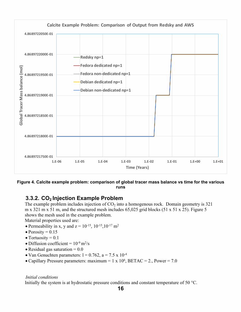
Computation time and results comparison Computing times on several AWS server setups were compared with Sandia’s RedSky, part of the high performance computing system. The Calcite example problem was run on several AWS instances with different operating systems, different Linux versions, two AWS tenancy options and “bind-to-socket” state. Table 1 shows the computation times for the various AWS runs were also compared to computation times of running the example problem on RedSky. Figure 4 shows “global tracer Mass balance” output vs time for the Calcite example problem, from the different AWS systems and RedSky. The results are virtually identical which indicates that the output were successfully reproduced on the various AWS systems.

15

Table 1. Simulation run times for the Calcite example problem

MPI Type

Linux Version OS

EC2 Instance1

Type

Cores(vCPUs)

Memory(GiBs) Tenancy np2

ComputeTime in Seconds

RedSky3 OpenMPI Fedora RHEL6 N/A N/A N/A N/A 1 1.52220E+02

AWS Open MPI Fedora

Amazon Linux AMI

2016.03.1 (HVM)

c4.8xlarge 36 60 Non dedicated 1 2.10660E+02

AWS Open MPI Fedora

Amazon Linux AMI

2016.03.1 (HVM)

c4.8xlarge 36 60 Dedicated Instance 1 2.12430E+02

AWS Open MPI Debian

Ubuntu Server 14.04 LTS

(HVM)

c4.8xlarge 36 60 Non dedicated 1 2.09950E+02

AWS Open MPI Debian

Ubuntu Server 14.04 LTS

(HVM)

c4.8xlarge 36 60 Dedicated Instance 1 2.08210E+02

1 See https://aws.amazon.com/ec2/instance-types/ for explanation of Amazon EC2 Instance Types2 np means number of processes and represents the number of processors used for an initiated program3 RedSky has 2846 nodes with 22768 cores; and 12 GB RAM per compute node

16

4.8689721750E-01

4.8689721800E-01

4.8689721850E-01

4.8689721900E-01

4.8689721950E-01

4.8689722000E-01

4.8689722050E-01

1.E-06 1.E-05 1.E-04 1.E-03 1.E-02 1.E-01 1.E+00 1.E+01

Glo

bal T

race

r Mas

s bal

ance

(mol

)

Time (Years)

Calcite Example Problem: Comparison of Output from Redsky and AWS

Redsky np=1

Fedora dedicated np=1

Fedora non-dedicated np=1

Debian dedicated np=1

Debian non-dedicated np=1

Figure 4. Calcite example problem: comparison of global tracer mass balance vs time for the various runs

3.3.2. CO2 Injection Example ProblemThe example problem includes injection of CO2 into a homogenous rock. Domain geometry is 321 m x 321 m x 51 m, and the structured mesh includes 65,025 grid blocks (51 x 51 x 25). Figure 5 shows the mesh used in the example problem.Material properties used are:Permeability in x, y and z = 10-15, 10-15,10-17 m2

Porosity = 0.15Tortuosity = 0.1Diffusion coefficient = 10-9 m2/sResidual gas saturation = 0.0Van Genuchten parameters: l = 0.762, a = 7.5 x 10-4

Capillary Pressure parameters: maximum = 1 x 106, BETAC = 2., Power = 7.0

Initial conditions Initially the system is at hydrostatic pressure conditions and constant temperature of 50 °C.

17

Boundary conditions At the top of the domain pressure is held constant at 20 MPa. CO2 is injected at a point (160, 160, 20) - (160,160,20). Rate of injection is: 1e-4 kg/s for 0.0 to 10.0 years. The injection is stopped after 10 years. A background concentration of 1e-6 mol/L is applied elsewhere in the domain.

For the simulation the PFLOTRAN numerical software (Hammond et al., 2014) was used. Use of PFLOTRAN allowed for high performance parallel computing utilizing many processors. Figures 6 shows CO2 concentration after simulation time of 5000 years.

Figure 5. Mesh for CO2 injection example problem with 65,025 grid blocks

Figure 6. Distribution of CO2 concentration after simulation time of 5000 years

18

Computation time and results comparisonComputing times on several AWS setups and Sandia’s RedSky, part of the high performance computing system, were also compared. The CO2 injection example problem was run on several AWS instances with different operating systems, different Linux versions, two AWS tenancy options and “bind-to-socket” state. The computation times for the various AWS runs were also compared to computation times of running the example problem on RedSky. The results are shown in Table 2.Figure 7 shows comparison of global CO2 mass in water phase vs time for the various runs for the CO2 injection example problem, from the different AWS systems and RedSky. The results are virtually identical which indicates that the output were successfully reproduced on the various AWS systems.

Table 2. Simulation run times for the CO2 injection example problem

MPI Type

Linux Version OS

EC2 Instance1

TypeCores

(vCPUs)Memory(GiBs) Tenancy np2

ComputeTime in Seconds

RedSky3 OpenMPI Fedora RHEL6 N/A N/A N/A N/A 1 4.14830E+02

AWS Open MPI Fedora

Amazon Linux AMI

2016.03.1 (HVM)

c4.8xlarge 36 60 Non dedicated 1 5.43390E+02

AWS Open MPI Fedora

Amazon Linux AMI

2016.03.1 (HVM)

c4.8xlarge 36 60 Dedicated Instance 1 5.33930E+02

AWS Open MPI Debian

Ubuntu Server 14.04 LTS

(HVM

c4.8xlarge 36 60 Non dedicated 1 5.29980E+02

AWS Open MPI Debian

Ubuntu Server 14.04 LTS

(HVM

c4.8xlarge 36 60 Dedicated Instance 1 1.41010E+03

1 See https://aws.amazon.com/ec2/instance-types/ for explanation of Amazon EC2 Instance Types2 np means number of processes and represents the number of processors used for an initiated program3 RedSky has 2846 nodes with 22768 cores; and 12 GB RAM per compute node

19

0

100

200

300

400

500

600

700

800

1.E-02 1.E-01 1.E+00 1.E+01 1.E+02 1.E+03 1.E+04

Glo

bal C

O2

Mas

s in

Wat

er P

hase

(km

ol)

Time (years)

Comparison of Output from Redsky and AWS - CO2 3D

Redsky np=1

Fedora dedicated np=1

Fedora non-dedicated np=1

Debian dedicated np=1

Debian non-dedicated np=1

Figure 7. CO2 injection example problem: comparison of global CO2 mass in water phase vs time for the various runs

Note: Results are nearly identical so graph lines overlap

20

3.4. Execution of Geohydrology and Nuclear Waste Problem

3.4.1. Example Problem for Flow and Transport in Fractured Granite RockThis public domain example problem is on flow and transport in fractured granite rock. The problem was selected to represent an actual modeling case for flow and transport in a generic high-level radioactive waste repository in fractured granite host rock. In the example permeability field is generated using the Fracture Continuum fracture characterization model (FCM) (Wang et al., 2016). A model domain of 1 km x 1 km x 1 km was used. For the FCM model a constant grid block size of 10 m x 10 m x 10 m was used, resulting in a mesh size of 106 grid blocks (Figure 8). Figure 9 shows the permeability field used in this example, which is one realization of the FCM method. Details such as fracture parameters and statistical data used for the different modeling tasks are described in Wang et al. (2016).

For this example, problem flow is driven from west to east (x=1 km) with a constant pressure of 1.001 MPa on the west face (x=0) and constant pressure of 1 MPa on the east face. The rest of the faces have no flow boundary conditions.

For the simulation the PFLOTRAN numerical software (Hammond et al., 2014) was used. Use of PFLOTRAN allowed for high performance parallel computing utilizing many processors. A flow run is first carried out to obtain steady state flow field. The fluxes from steady state flow are then used to drive the transport, and the breakthrough curve on the east face is calculated for comparing output of the different computing systems.

Figure 8. Mesh for granite example problem with 1,000,000 grid blocks

21

Figure 9. Permeability field for granite example problem with 1,000,000 grid blocks

Computation time and results comparison

Comparison was made of computing times on an AWS setup and Sandia’s Sky Bridge, part of the high performance computing system. The example problem was run on an AWS X1 instance type. The computation times for the various AWS runs were also compared to computation times of running the example problem on Sky Bridge. The results are shown in Table 3.

Figure 10 shows comparison of normalized breakthrough output on the east face vs time for the various runs for the granite example problem, from the AWS system and Sky Bridge. The results are identical which indicates that the output were successfully reproduced on the various AWS systems.

A second test problem was also used to compare results on Sandia’s Sky Bridge and an AWS instance. In this case the permeability field was replaced by a constant permeability of 5 x 10-17 m2. Flow and transport simulations were carried out on Sky Bridge and AWS. The results are shown in Table 4. Figure 11 shows comparison of normalized breakthrough output on the east face vs time for the various runs for the constant permeability granite example problem, from the AWS system and Sky Bridge. The results are identical which indicates the output was successfully reproduced on the various AWS systems.

22

Table 3. Simulation run times for the granite example problem with variable permeability

MPI Type

Linux Version OS

EC2 Instance1

Type

Cores(vCPUs)

Memory(GiBs) Tenancy np2

Compute Time in Hours

Sky Bridge3

OpenMPI Fedora RHEL6 N/A N/A N/A N/A 128 3.7853E-01

Gra

nite

Pro

blem

: T

rans

port

Run

AWS MPICH Fedora

Amazon Linux AMI

2016.03.1 (HVM)

x1.32xlarge 128 1952 Non dedicated 128 1.1042E+00

Table 4. Simulation run times for the granite example problem with constant permeability

MPI Type

Linux Version OS

EC2 Instance1

Type

Cores(vCPUs)

Memory(GiBs) Tenancy np2

Compute Time in Hours

Sky Bridge3

OpenMPI Fedora RHEL6 N/A N/A N/A N/A 128 .2774E+00

AWS MPICH Fedora

Amazon Linux AMI

2016.03.1 (HVM)

x1.32xlarge 128 1952 Non dedicated 128 1.6444E+00

Gra

nite

Pro

blem

: Fl

ow R

un

Sky Bridge3

OpenMPI Fedora RHEL6 N/A N/A N/A N/A 128 .27787E+00

Gra

nite

Pro

blem

: T

rans

port

Run

AWS MPICH Fedora

Amazon Linux AMI

2016.03.1 (HVM)

x1.32xlarge 128 1952 Non dedicated 128 1.9697E+00

1 See https://aws.amazon.com/ec2/instance-types/ for explanation of Amazon EC2 Instance Types2 np means number of processes and represents the number of processors used for an initiated program3 Sky Bridge has 1848 nodes with 29568 cores; and 64 GB RAM per compute node

23

0.0

0.1

0.2

0.3

0.4

0.5

0.6

0.7

0.8

0.9

1.0

1.E+00 1.E+01 1.E+02 1.E+03 1.E+04 1.E+05 1.E+06 1.E+07 1.E+08 1.E+09

Rela

tive

Bre

akth

roug

h at

Eas

t Fac

e

Time (years)

Breakthrough Curves at East Face of Domain for SNL HPC and AWS

Skybridge

AWS x1.32xlarge

Figure 10. Granite variable permeability example problem: comparison of relative breakthrough results vs time for AWS and Sky Bridge

Note: Results are nearly identical so graph lines overlap

24

0.0

0.1

0.2

0.3

0.4

0.5

0.6

0.7

0.8

0.9

1.0

1.E+00 1.E+01 1.E+02 1.E+03 1.E+04 1.E+05 1.E+06 1.E+07 1.E+08 1.E+09

Rela

tive

Bre

akth

roug

h at

Eas

t Fac

e

Time (years)

Breakthrough Curves at East Face of Domain for SNL HPC and AWS

Skybridge

AWS x1.32xlarge

Figure 11. Granite constant permeability example problem: comparison of relative breakthrough results vs time for AWS and Sky Bridge

Note: Results are nearly identical so graph lines overlap

25

4. RESULTS AND CONCLUSION

The objective of this study was to investigate the possibility of conducting numerical modeling relevant to geohydrology and nuclear waste disposal needs on the cloud. The results documented in this report demonstrate that large scale simulations can be efficiently executed on Amazon’s cloud system, AWS and that use of AWS is cost effective (Appendix C).

As part of the demonstration the open source numerical code PFLOTRAN was utilized to model porous medium example problems and a realistic problem on flow and transport in fractured crystalline rock, with a million grid blocks. The simulations were used to test a variety of AWS options (tenancy, Linux server types, capacity, etc.). Results were compared with Sandia based high performance computing platforms (RedSky and Sky Bridge). As shown in the report the outputs from cloud based simulations were identical with those from Sandia’s RedSky and Sky Bridge. By comparing run time and overall cost of the different AWS options the simulations demonstrated efficient and cost effective choices can be made for cloud computing.Recommendation for future work includes use of a multi-server system to allow modeling of larger problems in more reasonable amount of time. This would allow simulations of complex public domain problems not attempted in the current study. Future work should also include other test problems of importance to the geohydrology and nuclear waste disposal community.

Overall, the following was demonstrated: complex codes were readily run on the Amazon Web Services (AWS) infrastructure. complex codes were readily run on the AWS infrastructure using multiple servers (platforms) in

different configurations. runtimes for the trivial problems on different platforms can be materially differentone run of a public domain granite problem was compared to the same problem run on SNL’s on

premises Sky Bridge HPC. The problem was computed in AWS using a single node with 1,952 GiB of DDR4 based memory and 128 virtual processors.

This demonstration accomplished its goals. Future work should focus on resolving technical issues related to executing complex codes employing multiple computing nodes, and addressing frequently expressed, but not necessarily supported, security concerns about running codes and problems considered to be OUO in the cloud.

Insight into persistent problems inherently associated with complex compliance calculations was gained. Appendix C presents other useful observations drawn from the project. Also, an ancillary concern related to performing such calculations in the Cloud is that depending on how one configures the server instance(s) one may not know specifically what hardware is being used (and where it is located) to perform the calculation. This uncertainty may or may not influence the results of the calculation.

26

5. REFERENCES

Amazon Web Services https://aws.amazon.com

AWS, Overview of Security Processes, Amazon Web Services, June 2016.

Hammond, G.E., P.C. Lichtner and R.T. Mills, 2014. Evaluating the Performance of Parallel Subsurface Simulators: An Illustrative Example with PFLOTRAN, Water Resources Research, 50, doi:10.1002/2012WR013483.

Y. Wang, T. Hadgu, E. A. Kalinina, J. Jerden, J. M. Copple, T. Cruse, and W. Ebert , E. Buck, R. Eittman, R. Tinnacher, C. Tournassat, J. Davis, H. Viswanathan, S. Chu, T. Dittrich, F. Hyman, S. Karra, N. Makedonska, P. Reimus, M. Zavarin, C. Joseph, (2016), Used Fuel Disposition in Crystalline Rocks: FY16 Progress Report, FCRD-UFD-2016-000076, SAND2016-9297 R. U.S. Department of Energy, Used Fuel Disposition R&D Campaign

27

Appendix A - Guide to Launching a Virtual Machine on AWSLog into AWS Web Consolehttps://console.aws.amazon.com/

Create EC2 InstanceThe Amazon Web Services directory dashboard lists provided services and service productsClick on EC2 under ComputeClick the Launch Instance buttonYou will be brought to Step 1: Choose an Amazon Machine Image (AMI)

(please read the ‘Additional Information’ in the right panel)o Select the Amazon Linux 64 Bit AMI HVM SSD Volume AMI (it should be the first AMI

listed) under the Quick Start menuNext Step 2: Choose an Instance Type (please read the information at the ‘Learn More’ hyperlink)o A long listing of Instance Types accompanied with associated attributes will be displayedo Click on c4.8xlarge typeThe checkbox at the far left of the row should be filled ino Click on the Next: Configure Instance Details buttono Next Step 3: Configure Instance Details (Details relating to the instance will be provided)o Select enable for Auto-assign public IPo Click the Next: Add Storage buttonNext Step 4: Add Storage (please read the information at the ‘Learn More’ hyperlink)o Storage specifications for the instance will be listed o Ensure Delete on Termination is checked and keep the default Size and Volume Typeo Click the Next: Tag Instance buttonNext Step 5: Tag Instance (please read the information at the ‘Learn More’ hyperlink)o Two columns will be displayed: Key and Valueo A row will be displayed under the column headerso Enter the text Instance Name into the row's second column

Ensure Name is in the row's first column textboxo Click the Next: Configure Security Group buttonNext Step 6: Configure Security Group (please read the information at the ‘Learn More’ hyperlink)o Ensure the Create a new security group radio button is selected for Assign a security groupo Enter Security Group Name for the Security group nameo Enter Security Group Name for the Descriptiono Ensure a default rule Type is SSH and Source is Custom IP with the Public IP you will be accessing the instance from along with /32 (X.X.X.X/32)o Click Review and LaunchNext Step 7: Review Instance Launcho The previous steps and selections will be displayed for reviewo Ensure proper selections were madeo Click the Launch buttonNext Select an existing key pair or create a new key pair o Select Create a new key pair o Enter KeyPair in the textbox for the Key pair nameo Click the Download Key Pair buttono After the key pair is downloaded, click the Launch Instances button

28

SSH to the EC2 InstanceThe Launch Status will be displayed along with additional informationo Click the View Instances buttono All instances will be displayed with additional informationo Enter Instance Name in the filter textbox field o When the Status Check is displayed as 2/2 checks passed, click on your instanceo Another pane will display attributes associated to the instance, find the Public IPo SSH to your new instance ssh –i /location/to/your/keypair.pem ec2-user@Public IP (replace the

Public IP with the actual public IP of the created Instance)

29

Appendix B - Observations from the Demonstration Project

SecurityOne source of persistent resistance to using commercial cloud services revolves around security (i.e. upload and accessibility of OUO (or CUI) materials to the cloud). This seems to be mostly a ‘red herring’, since access to a cloud server instance can be restricted to an individual port for a specific IP address. The only more secure connection is no connection at all.

This demonstration used a Federal Risk and Authorization Management Program (FedRAMP) approved region in AWS. Note that all AWS regions located inside the United States are FedRAMP approved at a moderate impact level. Additionally, there is an ITAR and FedRAMP approved region called GovCloud. Because it was not available at the time the demonstration account was established, investigating this region was outside of the scope of the project. However, initial examination suggests AWS GovCloud may address most serious security concerns (Appendix D, and AWS, 2016). If available at the time the AWS account was established, it would have been preferable to associate the account with AWS GovCloud (US) to remove most, if not all, related security questions. This approach should be taken in future endeavors.

For expediency, the demonstration took an approach that avoided the entire security question and did not avail ourselves of any of the advanced security features offered by AWS because:PFLOTRAN is an open source, massively parallel subsurface flow and reactive transport code.The calculation used PFLOTRAN to solve flow and transport problems simulated in generic fractured

crystalline rock, and the simulations are public domain.

Amazon EC2 works in conjunction with Amazon VPC to provide security and robust networking functionality for compute resources (https://aws.amazon.com/ec2/).AWS compute instances are located in a Virtual Private Cloud (VPC) with an IP range that you specify.

You decide which instances are exposed to the Internet and which remain private.Security Groups and networks ACLs allow you to control inbound and outbound network access to and

from your instances.You can connect your existing IT infrastructure to resources in your VPC using industry-standard

encrypted IPsec VPN connections.For additional isolation, you can provision your EC2 resources on Dedicated Hosts or as Dedicated

Instances. Both allow you to use EC2 instances in a VPC on hardware dedicated to a single customer.

Amazon Virtual Private Cloud (https://aws.amazon.com/vpc/) This service allows one to provision a logically isolated section of the Amazon Web Services (AWS) cloud where the user can launch AWS resources in a virtual user defined network. Complete control over the virtual networking environment is allowed, including selection of an IP address range, creation of subnets, and configuration of route tables and network gateways.

The network for the Amazon Virtual Private Cloud is easily configured. Multiple layers of security can be leveraged, including security groups and network access control lists, to help control access to Amazon EC2 instances in each subnet. Additionally, Hardware Virtual Private Network (VPN) connections between your corporate datacenter and your VPC can be created to leverage the AWS cloud as an extension of a corporate datacenter.

30

Steps to launching a server instance on AWSChoose an Amazon Machine Image (AMI) - An AMI is a template that contains the software

configuration (operating system, application server, and applications) required to launch the instance. One can select an AMI provided by AWS, our user community, or the AWS Marketplace; or you can select one of your own AMIs.

Choose an Instance Type Amazon - EC2 provides a wide selection of instance types optimized to fit different use cases. Instances are virtual servers that can run applications. They have varying combinations of CPU, memory, storage, and networking capacity, and provide the flexibility to choose the appropriate mix of resources for given applications.

Configure Instance Details - Configure the instance to suit your requirements. One can launch multiple instances from the same AMI.

Add Storage – The subject instance will be launched with the specified storage device settings. One can attach additional EBS volumes and instance store volumes to your instance, or edit the settings of the root volume.

Tag Instance - A tag consists of a case-sensitive key-value pair. For example, one could define a tag with key = Name and value = Webserver. This can be used to uniquely name the subject instance.

Configure Security Group - A security group is a set of firewall rules that control the traffic for the specific instance. One can add rules to allow specific traffic to reach your instance.

Review - This allows review of the instance launch details. One can edit changes for each section.Launch Click Launch to assign a key pair to your instance and complete the launch process.

Multiple server instances can be selected, configured, launched and displayed as shown in Figure 12.

Figure 12 Example of EC2 Server Instances Panel

Launching a server instance involves use of complex private keys as shown in Figure 13, adding to assurances of secure access to server instances.

31

Figure 13 Example of a Private Key

AWS ACCOUNT ADMINISTRATIONAccess to AWS is easily established by setting up an account at https://aws.amazon.com/. One needs to provide a verifiable (Sandia) email address and a means of payment (credit card or P-Card). This established the account root credentials. Credentials for users can then be set up using Identity and Access Management (IAM). Root credentials allow the user to access billing related information, but AWS encourages using a separate credential for working within the account. Billing is straightforward and invoices explicitly identify the source(s) of charges (Figure 14). Also, AWS billing and cost management details (Figures 15 and 16) are very helpful.

The account used for this demonstration was set up to charge to a P-Card. Be sure to work with the P-Card owner and procurement to set up the details. It is recommended that payment method be a P-Card. While this is allowable under SNL procurement rules, it needs to be backed up with someone’s Corporate Credit Card to account for unusual circumstances arise.

Be very careful to assure that server instances are not left in “Instance State Running”. Charges will be applied for servers left in this state. While one of AWS’ slogans is that ‘you only pay for what you use’, the converse is also true. If you leave server instances in an active state, you will pay for using them even if they are not computing. This can be expensive when being charged $10-15/hour of server time. Further, even if all server instances are left in “Instance State Stopped” you may still incur charges for services like storage and static IP addresses. While the hourly rates for these items are certainly not as expensive as server time, it can add up. For example, a modest amount of

32

storage could cost several hundred dollars a month. AWS makes monitoring billing and cost management straightforward (Figures 15, and 16), but you must monitor it to avoid surprises.

Figure 14 Example Invoice

33

Figure 15 AWS Billing and Cost Management Example

Figure 16 AWS Billing and Cost Management Detail Example

34

AWS COSTS for this Demonstration – AWS costs from February through September was $2210.95. For perspective that is about 22 hours of SNL-IT MOW unburdened time and 0.005 of the cost of the new TSPA server installed by 6220 in 2014.

AWS COSTS VS. ON-PREMISES HPCFigure 17 is a CPU equivalent comparison of the cost of cloud-based servers versus the on-premises YMP TSPA server cluster (Cl-2014). This comparison addresses only the annualized costs of the equipment itself and does not include personnel costs, which are considered equivalent. The cost of the YM TSPA server cluster was about $300,000 plus installation and networking, and typically has been replaced about every four years. For this analysis an annualized cost ranging from about $100,000 to $125,000 is assumed. Such a server cluster has 640 CPUs whereas each AWS server chosen for the analysis has 128 vCPUs (virtual CPUs), a difference of a factor of five. Hence the CPU equivalent of the YM TSPA server cluster annual cost is about $20,000 to $25,000 for the purposes of comparison to the specified AWS servers.

To exceed this cost range ($20,000 to $25,000) one would need to run the most expensive AWS server, (Microsoft_x1.32large) for over 1300 hours (about 8 weeks) per year and the Linux_x1.32xlarge server for over 1875 hours (about 11 weeks) per year. This is a most conservative comparison, as it considers only ‘On-demand’ servers, the most expensive variety available on AWS. There are extensive server and pricing options available on AWS. For example, use of ‘reserved instances’ could reduce AWS server costs by 20-30% with little commitment, and up to 75% with substantial commitment. Reserved instances are a pricing option for EC2 instances that discounts the on-demand usage charge for instances that meet the specified parameters. However, customers pay for the entire term of the instance, regardless of how they use it.

Figure 17 On Premises vs AWS On Demand Server Costs (CPU-equivalent)

35

Potential Positive Influences on Regulatory CalculationsA common and reoccurring conundrum inherent to complex regulatory compliance calculations, such as that have occurred in the context of both the Waste Isolation Pilot Plant (WIPP) and Yucca Mountain (YM) projects consists of:The compliance calculation is performed based on an on-premises software and hardware configuration,

presented to a regulator and accepted as the basis for their affirmative action.Time (years) passes and the software used for the calculation changes (is upgraded) and/or the hardware

transitions to obsolescence or otherwise requires replacement.Much effort is expended re-establishing and re-running the compliance calculation to demonstrate that

the initial result, on which the regulatory action was based, can be reproduced with fidelity using the new/upgraded software/hardware configuration.

Hardware changes are often perceived as a potential source of possible influence on the calculation

The results of this demonstration illustrate that:Calculation results are effectively identical, and independent of the server type (platform) and how it is

configured (shared or dedicated). This could be important in terms of convincing a regulator that within certain constraints, hardware has little impact on the results.

AMIs (Amazon Machine Images) have potentially great value on a rigorously regulated program. AMI’s provide an exact image of the compliance code state (software, operating system configuration, data, etc.) at the time results are recorded. Preservation of the “AMI of record” would provide a valuable baseline and could provide a readily accessed “copy” of the original calculation to serve as a basis of comparison for proposed calculation additions or changes.

36

Appendix C - AWS GovCloud InformationInformation below is from https://aws.amazon.com/govcloud-us/ and https://aws.amazon.com/govcloud-us/security/.

37

38

6. DISTRIBUTION

1 MS 0736 Tito Bonano 62201 MS 0747 Kevin McMahon 62221 MS 0747 Bob MacKinnon 62241 MS 0747 Gordon Appel 62221 MS 0747 Teklu Hadgu 62221 MS 0747 Glenn Edward Hammond 62241 MS 0747 Emily Stein 62241 MS 0747 Jennifer M. Frederick 62241 MS 0747 Paul Mariner 62241 MS 0779 Yifeng Want 62221 MS 0779 Carlos Jove-Colon 62221 MS 1395 Paul Shoemaker 69301 MS 1488 John Gifford Miner 90131 MS 1488 John J. Jones 95411 MS 1488 Brandon Thorin Klein 95411 MS 0899 Technical Library 9536 (electronic copy)