comp3421 - unsw engineering

COMP3421Particle Systems, Rasterisation

Particle systems

Some visual phenomena are best modelled

as collections of small particles.

Examples: rain, snow, fire, smoke, dust

Particle systems

Particles are usually represented as small

textured quads or point sprites – single

vertices with an image attached.

They are billboarded, i.e transformed so

that they are always face towards the

camera.

Billboarding

Particle systems

Particles are created by an emitter object

and evolve over time, usually changing

position, size, colour.

emitter

Particle evolutionUsually the rules for particle evolution are

simple local equations:

interpolate from one colour to another

over time

move with constant speed or

acceleration.

To simulate many particles it is important

these update steps are kept simple and

fast.

Particles on the GPU

Particle systems are well suited to

implementation as vertex shaders.

The particles can be represented as

individual point vertices.

A vertex shader can compute the position

of each particle at each moment in time.

Particle Systemuniform vec3 vel;

uniform float g, m, t;

void main(){

vec3 pos;

pos.x = gl_Vertex.x + vel.x*t;

pos.y = gl_Vertex.y + vel.y*t

+ g/(2.0*m)*t*t;

pos.z = gl_Vertex.z + vel.z*t;

gl_Position =

ModelViewProjectionMatrix*vec4(pos,1);

}

The graphics pipeline

Projection

transformationIllumination

ClippingPerspective

divisionViewportRasterisation

TexturingFrame

bufferDisplay

Hidden

surface

removal

Model-View Transform

Model

Transform

View

Transform

Model

User

Rasterisation

Rasterisation is the process of converting

lines and polygons represented by their

vertices into fragments.

Fragments are like pixels but include color,

depth, texture coordinate. They may also

never make it to the screen due to hidden

surface removal or culling.

Rasterisation

This operation needs to be accurate and

efficient.

For this reason we prefer to use simple

integer calculations.

All are calculations are now in 2D screen

space.

Drawing lines

(x0, y0)

(x1, y1)

(x, y)

Drawing lines - bad

double m = (y1-y0)/(double)(x1-

x0);

double b = y0 - m * x0;

for (int x = x0; x <= x1; x++) {

int y = round(m * x + b);

drawPixel(x, y);

}

Problems• Floating point math is slow and

creates rounding errors•Floating point multiplication, addition and round for each pixel

• Code does not consider:•Points are not connected if m > 1

•Divide by zero if x0 == x1 (vertical lines)

•Doesn't work if x0 > x1

Example: y = 2x

Incremental – still

bad// incremental algorithm

double m = (y1-y0)/(double)(x1-x0);

double y = y0;

for (int x = x0; x <= x1; x++) {

y += m; //one less multiplication

drawPixel(x, round(y));

}

Bresenham's

algorithmWe want to draw lines using only integer

calculations and avoid multiplications.

Such an algorithm is suitable for fast

implementation in hardware.

The key idea is that calculations are done

incrementally, based on the values for the

previous pixel.

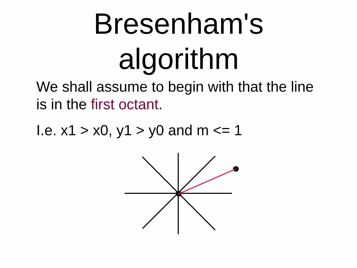
Bresenham's

algorithmWe shall assume to begin with that the line

is in the first octant.

I.e. x1 > x0, y1 > y0 and m <= 1

Bresenham’s IdeaFor each x we work out which pixel we set next

The next pixel with the same y value

if the line passes below the midpoint

between the two pixels

Or the next pixel with an increased y value

if the line passes above the midpoint

between the two pixels

Bresenham's

algorithm

P (xi, yi)

M

L (xi+1, yi)

U (xi+1, yi+1)

M1

M2

Pseudocode

int y = y0;

for (int x = x0; x <= x1; x++) {

setPixel(x,y);

M = (x + 1, y + 1/2)

if (M is below the line)

y++

}

Testing above/below

M is a float and we do not want to actually

calculate it.

Incrementally

Completeint y = y0;

int w = x1 - x0; int h = y1 - y0;

int F = 2 * h - w;

for (int x = x0; x <= x1; x++) {

setPixel(x,y);

if (F < 0) F += 2*h;

else {

F += 2*(h-w); y++;

}

}

Example

x y F

0 0 2

1 1 -4

2 1 6

3 2 0

4 3 -6

5 3 4

6 4 -2

7 4 8

8 5 2

(0,0)

(8,5)

w = 8

h = 5

Relaxing restrictions

Lines in the other quadrants can be drawn

by symmetrical versions of the algorithm.

We need to be careful that drawing from P

to Q and from Q to P set the same pixels.

Horizontal and vertical lines are common

enough to warrant their own optimised

code.

Polygon fillingDetermining which pixels are inside a

polygon is a matter of applying the edge-

crossing test (from week 3) for each

possible pixel.

Shared edgesPixels on shared edges between polygons

need to be draw consistently regardless of

the order the polygons are drawn, with no

gaps.

We adopt a rule:

The edge pixels belong to the rightmost

and/or upper polygon ie Do not draw

rightmost or uppermost edge pixels

Scanline algorithm

Testing every pixel is very inefficient.

We only need to check where the result

changes value, i.e. when we cross an edge.

We proceed row by row:

Calculate intersections incrementally.

Sort by x value.

Fill runs of pixels between intersections.

Active Edge List

We keep a list of active edges that overlap

the current scanline.

Edges are added to the list as we pass the

bottom vertex.

Edges are removed from the list as we

pass the top vertex.

The edge intersection is updated

incrementally.

Edges

For each edge in the AEL we store:

The x value of its crossing with the current

row (initially the bottom x value)

The amount the x value changes from row-

to-row (1/gradient)

The y value of the top vertex.

Edge table

The (inactive) edge table is a lookup table

index on the y-value of the lower vertex of

the edge.

This allows for fast addition of new edges.

Horizontal edges are not added

In this list we store the initial values needed

in the active edge list as well as the

starting y value for the edge.

//For every scanline

for (y = minY; y <= maxY; y++){

remove all edges that end at y

for (Edge e : active) {

e.x = e.x + e.inc;

}

add all edges that start at y – keep list

sorted by x

for (int i=0; i < active.size; i+=2){

fillPixels(active[i].x, active[i+1].x,y);

}

}

Example

y in x inc y out

0 1 -0.25 4

0 5 1 1

0 9 -3 1

0 9 -0.4 5

3 2 -2 4

3 2 2.5 5(0,0)

Edge table

Example

x inc y out

1 -0.25 4

5 1 1

9 -3 1

9 -0.4 5

Active edge list

y=0

Example

x inc y out

0.75 -0.25 4

8.6 -0.4 5

Active edge list

y=1

Example

x inc y out

0.5 -0.25 4

8.2 -0.4 5

Active edge list

y=2

Example

x inc y out

0.25 -0.25 4

2 -2 4

2 2.5 5

7.8 -0.4 5

Active edge list

y=3

Example

x inc y out

4.5 2.5 5

7.4 -0.4 5

Active edge list

y=4

Example

x inc y out

Active edge list

y=5

OpenGLOpenGL is optimised for implementation on

hardware.

Hardware implementations do not work well

with variable length lists.

So OpenGL enforces polygons to be

convex. This means the active edge list

always has 2 entries.

More complex polygons need to be

tessellated into simple convex pieces.

AliasingLines and polygons drawn with these

algorithms tend to look jagged if the pixel

size is too large.

This is another form of aliasing.

AntialiasingThere are two basic approaches to

eliminating aliasing (antialiasing).

Prefiltering is computing exact pixel values

geometrically rather than by sampling.

Postfiltering is taking samples at a higher

resolution (supersampling) and then

averaging.

Prefiltering

0 0 0 0.2 0.7 0.5

0.1 0.4 0.8 0.9 0.5 0.1

0.5 0.7 0.3 0 0 0

For each pixel, compute the amount

occupied and set pixel value to that

percentage.

Prefiltering

0.9

For each pixel, compute the amount

occupied and set pixel value to that

percentage.

Postfiltering

Draw the line at a higher resolution and

average (supersampling).

Postfiltering


average (supersampling)

Postfiltering


average (supersampling).

Weighted postfiltering

It is common to apply weights to the

samples to favour values in the center of

the pixel.

1/16 1/16 1/16

1/16 1/2 1/16

1/16 1/16 1/16

Stochastic samplingTaking supersamples in a grid still tends to

produce noticeably regular aliasing effects.

Adding small amounts of jitter to the

sampled points makes aliasing effects

appear as visual noise.

Adaptive Sampling

Supersampling in large areas of uniform

colour is wasteful.

Supersampling is most useful in areas of

major colour change.

Solution: Sample recursively, at finer levels

of detail in areas with more colour variance.

Adaptive sampling

Samples

Adaptive sampling

Antialiasing

Prefiltering is most accurate but requires

more computation.

Postfiltering can be faster. Accuracy

depends on how many samples are taken

per pixel. More samples means larger

memory usage.

OpenGL

// implementation dependant may not

even do anything

gl.glEnable(GL2.GL_LINE_SMOOTH);

gl.glHint(GL2.GL_LINE_SMOOTH_HINT,G

L2.GL_NICEST);

// also requires alpha blending

gl.glEnable(GL2.GL_BLEND);

gl.glBlendFunc(GL2.GL_SRC_ALPHA,

GL2.GL_ONE_MINUS_SRC_ALPHA);

OpenGL

// full-screen multi-sampling

GLCapabilities capabilities =

new GLCapabilities();

capabilities.setNumSamples(4);

capabilities.setSampleBuffers(tr

ue);

// ...

gl.glEnable(GL.GL_MULTISAMPLE);

comp3421 - unsw engineering

Documents