comparison of readability indices with grades 1-5 ... · comparison of readability indices with...
TRANSCRIPT

COMPARISON OF READABILITY INDICES WITH GRADES 1-5 NARRATIVE AND
EXPOSITORY TEXTS
by
SUSAN HARDEN
DISSERTATION
Submitted to the Graduate School
of Wayne State University,
Detroit, Michigan
in partial fulfillment of the requirements
for the degree of
DOCTOR OF PHILOSOPHY
2018
MAJOR: EDUCATIONAL EVALUATION AND
RESEARCH
Approved By:
Advisor Date

© COPYRIGHT BY
SUSAN HARDEN 2018
All Rights Reserved

ii
DEDICATION
This dissertation is dedicated to my family, the ones who have provided constant support
of the time and energy I have put into this work. To my husband Eric W. Harden, who has not only
supported me emotionally and intellectually, but also selflessly provided the financial support for
this endeavor.
To my children, Faith, Lauren and Andrew, who have sacrificed much to allow me to spend
the time and energy required to complete this work. I love you to Heaven and back for allowing
me to reach this goal!
To my mother, Janet Rohde, who has encouraged me regularly to keep pressing on and
finish strong. Your constant support is greatly appreciated. I have learned the importance of a great
education from you.
And finally, to the memory of my father, Robert Rohde and my grandmother, Grace Baker.
I miss you both terribly but still feel your love and support daily.
iii
ACKNOWLEDGMENTS
This journey would not have been possible without the encouragement, teaching, and
support of Dr. Shlomo Sawilowsky. Dr. Sawilowsky started me on the path to this degree and he
has seen me through until the end. I am truly thankful for all the time and knowledge he has
bestowed upon me during this process.
And to my committee members (Dr. Jazlin Ebenezer, Dr. Monte Piliawsky, and Dr.
Elizabeth McQuillen), I thank you for your willingness to mentor me through this process. Your
guidance and input have been priceless. You each bestowed upon me great knowledge and have
helped me grow academically.

iv
TABLE OF CONTENTS
DEDICATION ................................................................................................................................ ii
ACKNOWLEDGMENTS ............................................................................................................. iii
LIST OF TABLES ........................................................................................................................ vii
LIST OF FIGURES ..................................................................................................................... viii
CHAPTER 1 ................................................................................................................................... 1
Motivation and Interest ............................................................................................................... 3
Text Complexity ........................................................................................................................... 4
Readability .................................................................................................................................. 6
Statement of the Problem ............................................................................................................ 8
Purpose of the study .................................................................................................................... 9
Assumptions and Limitations .................................................................................................... 10
CHAPTER 2 “Review of Literature” ........................................................................................... 12
Policy ......................................................................................................................................... 21
Readability ................................................................................................................................ 23
Text Readability Formulas and Text Simplification .................................................................. 28
Text Complexity ......................................................................................................................... 33
CHAPTER 3 “Methodology” ....................................................................................................... 36

v
Design and Sample .................................................................................................................... 36
Agreement and Bland-Altman Method ...................................................................................... 38
Reliability of Readability Indices .............................................................................................. 40
Data Analysis ............................................................................................................................ 43
CHAPTER 4 “Results” ................................................................................................................. 46
Unintended Findings ................................................................................................................. 46
Analysis ..................................................................................................................................... 46
Spache vs. Gunning Fog............................................................................................................ 48
Flesch-Kincaid Grade Level vs. Fry Graph .............................................................................. 52
Flesch-Kincaid Grade Level vs. Dale-Chall ............................................................................. 55
Flesch-Kincaid Grade Level vs. Spache ................................................................................... 57
Flesch-Kincaid Grade Level vs. Gunning Fog.......................................................................... 60
Flesch-Kincaid Grade Level vs. Smog ...................................................................................... 62
Fry Graph vs. Dale-Chall ......................................................................................................... 64
Fry Graph vs. Spache ................................................................................................................ 67
Fry Graph vs. Gunning Fog ...................................................................................................... 69
Fry Graph vs. Smog .................................................................................................................. 72
Dale-Chall vs. Spache ............................................................................................................... 74
Dale-Chall vs. Gunning Fog ..................................................................................................... 77

vi
Dale-Chall vs. Smog .................................................................................................................. 79
Spache vs. Smog ........................................................................................................................ 82
Gunning Fog vs. Smog .............................................................................................................. 84
CHAPTER 5 “Conclusions and Recommendations” ................................................................... 87
Limitations of the Study ............................................................................................................. 91
Further Research....................................................................................................................... 92
APPENDIX A: BLAND-ALTMAN PLOTS FOR INDIVIDUAL GRADE LEVELS AND
GENRES ....................................................................................................................................... 94
APPENDIX B: BLAND-ALTMAN PLOTS BY GENRE, ALL GRADE LEVELS ................ 114
REFERENCES ........................................................................................................................... 125
ABSTRACT ................................................................................................................................ 135
AUTOBIOGRAPHICAL STATEMENT ................................................................................... 136

vii
LIST OF TABLES
Table 1: Articles Included in Review of Literature. ..................................................................... 12
Table 2: Critical Analysis of Literature Review Articles ............................................................. 13
Table 3: Key Questions for Literature Review ............................................................................. 18
Table 4: Computational Formulas for Reading Indexes ............................................................... 36
Table 5: Paired Readability Indices to Determine Agreement Using Bland-Altman Plots .......... 44
Table 6: Reading Passage Sample Size ........................................................................................ 47
Table 7: Spache vs Gunning Fog .................................................................................................. 49
Table 8: Flesch-Kincaid Grade Level vs. Fry Graph .................................................................... 53
Table 9: Flesch-Kincaid Grade Level vs. Dale-Chall ................................................................... 55
Table 10: Flesch-Kincaid Grade Level vs. Spache ....................................................................... 58
Table 11: Flesch-Kincaid Grade Level vs. Gunning Fog ............................................................. 60
Table 12: Flesch-Kincaid Grade Level vs. Smog ......................................................................... 62
Table 13: Fry Graph vs. Dale-Chall .............................................................................................. 65
Table 14: Fry Graph vs. Spache .................................................................................................... 67
Table 15: Fry Graph vs. Gunning Fog .......................................................................................... 70
Table 16: Fry Graph vs. Smog ...................................................................................................... 72
Table 17: Dale-Chall vs. Spache ................................................................................................... 75
Table 18: Dale-Chall vs. Gunning Fog ......................................................................................... 77
Table 19: Dale-Chall vs. Smog ..................................................................................................... 79
Table 20: Spache vs Smog ............................................................................................................ 82
Table 21: Gunning Fog vs Smog .................................................................................................. 84

viii
LIST OF FIGURES
Figure 1: Venn Diagram of Reading Comprehension Factors .................................................................... 7
Figure 2: Common Core State Standards Model of Text Complexity ..................................................... 21
Figure 3: Sample Bland-Altman Plot ........................................................................................................ 39
Figure 4. Fiction Grade 1-5 Spache-Gunning Fog Bland-Altman Plot .................................................... 50
Figure 5. Non-Fiction Grade 1-5 Spache-Gunning Fog Bland-Altman Plot ............................................ 50
Figure 6. Fiction Grade 3 Spache-Gunning Fog Bland-Altman Plot........................................................ 51
Figure 7. Non-Fiction Grade 2 Spache-Gunning Fog Bland-Altman Plot ............................................... 51
Figure 8. Non-Fiction Grade 4 Spache-Gunning Fog Bland-Altman Plot ............................................... 52
Figure 9. Fiction Grade 1 Flesch-Kincaid Grade Level-Fry Graph Bland-Altman Plot .......................... 54
Figure 10. Fiction Grade 2 Flesch-Kincaid Grade Level-Fry Graph Bland-Altman Plot ........................ 54
Figure 11. Non-Fiction Grade 3 Flesch-Kincaid Grade Level-Fry Graph Bland-Altman Plot ................ 55
Figure 12. Fiction Grade 3 Flesch-Kincaid Grade Level-Dale-Chall Bland-Altman Plot ....................... 56
Figure 13. Non-Fiction Grade 4 Flesch-Kincaid Grade Level-Dale-Chall Bland-Altman Plot ............... 57
Figure 14. Non-Fiction Grade 5 Flesch-Kincaid Grade Level-Dale-Chall Bland-Altman Plot ............... 57
Figure 15. Fiction Grade 1 Flesch-Kincaid Grade Level-Spache Bland-Altman Plot ............................. 59
Figure 16. Fiction Grade 5 Flesch-Kincaid Grade Level-Spache Bland-Altman Plot ............................. 59
Figure 17. Non-Fiction Grade 4 Flesch-Kincaid Grade Level-Spache Bland-Altman Plot ..................... 60
Figure 18. Fiction Grade 5 Flesch-Kincaid Grade Level-Gunning Fog Bland-Altman Plot .................... 62
Figure 19. Fiction Grade 3 Flesch-Kincaid Grade Level-Gunning Fog Bland-Altman Plot .................... 62
Figure 20. Non-Fiction Grade 3 Flesch-Kincaid Grade Level-Gunning Fog Bland-Altman Plot ............ 62
Figure 21. Non-Fiction Grade 3 Flesch-Kincaid Grade Level-Smog Bland-Altman Plot ....................... 64
Figure 22. Non-Fiction Grade 4 Flesch-Kincaid Grade Level-Smog Bland Altman Plot ........................ 64

ix
Figure 23. Fiction Grade 4 Fry Graph-Dale-Chall Bland-Altman Plot .................................................... 66
Figure 24. Non-Fiction Grade 3 Fry Graph-Dale-Chall Bland-Altman Plot ............................................ 66
Figure 25. Non-Fiction Grade 5 Fry Graph-Dale-Chall Bland-Altman Plot ............................................ 67
Figure 26. Fiction Grade 1 Fry Graph-Spache Bland-Altman Plot .......................................................... 68
Figure 27. Non-Fiction Grade 1 Fry Graph-Spache Bland-Altman Plot .................................................. 69
Figure 28. Non-Fiction Grade 2 Fry Graph-Spache Bland-Altman Plot .................................................. 69
Figure 29. Fiction Grade 5 Fry Graph-Gunning Fog Bland-Altman Plot................................................. 71
Figure 30. Non-Fiction Grade 2 Fry Graph-Gunning Fog Bland-Altman Plot ........................................ 71
Figure 31. Non-Fiction Grade 3 Fry Graph-Gunning Fog Bland-Altman Plot ........................................ 72
Figure 32. Fiction Grade 1 Fry Graph-Smog Bland-Altman Plot ............................................................ 73
Figure 33. Fiction Grade 5 Fry Graph-Smog Bland-Altman Plot ............................................................ 74
Figure 34. Non-Fiction Grade 3 Fry Graph-Smog Bland-Altman Plot .................................................... 74
Figure 35. Non-Fiction Grade 1 Dale-Chall-Spache Bland-Altman Plot ................................................. 76
Figure 36. Non-Fiction Grade 3 Dale-Chall-Spache Bland-Altman Plot ................................................. 76
Figure 37. Fiction Grade 4 Dale-Chall-Spache Bland-Altman plot ......................................................... 77
Figure 38. Fiction Grade 2 Dale-Chall-Gunning Fog Bland-Altman Plot................................................ 78
Figure 39. Non-Fiction Grade 2 Dale-Chall-Gunning Fog Bland-Altman Plot ....................................... 79
Figure 40. Non-Fiction Grade 4 Dale-Chall-Gunning Fog Bland-Altman Plot ....................................... 79
Figure 41. Fiction Grade 1 Dale-Chall-Smog Bland-Altman Plot ........................................................... 81
Figure 42. Non-Fiction Grade 1 Dale-Chall-Smog Bland-Altman Plot ................................................... 81
Figure 43. Non-Fiction Grade 4 Dale-Chall-Smog Bland-Altman Plot ................................................... 82
Figure 44. Fiction Grade 4 Spache-Smog Bland-Altman Plot ................................................................. 83
Figure 45. Non-Fiction Grade 2 Spache-Smog Bland-Altman Plot ......................................................... 83

x
Figure 46. Non-Fiction Grade 3 Spache-Smog Bland-Altman Plot ......................................................... 84
Figure 47. Non-Fiction Grade 3 Gunning Fog-Smog Bland-Altman Plot ................................................ 86
Figure 48. Fiction Grade 2 Gunning Fog-Smog Bland-Altman Plot ........................................................ 86
Figure 49. Fiction Grade 5 Gunning Fog-Smog Bland-Altman Plot ........................................................ 86
Figure 50. Fry Graph Plot Example. ......................................................................................................... 89

1
CHAPTER 1
Reading is an act of recitation and a process that requires comprehension of the written
word. Reading comprehension requires complex interactions with a text, i.e., engagement in a
constant internal dialogue to make meaning from the written word (Zimmerman & Hutchins,
2003). Many factors contribute to reading comprehension, such as (a) ability to process and
understand syntactic, semantic, and graphophonemic information (Hittleman, 1973) which include
word difficulty and sentence length (Fry, 1975; Crossley, Allen, & McNamara, 2011), (b)
motivation (Moley, Bandre, & George, 2011; Guthrie, et al., 2006; Logan, Medford, & Hughes,
2011) and (c) ability to decipher text elements such as pictures and diagrams (Gallagher, Fazio, &
Gunning, 2012), as related to text complexity.
Hittleman (1973) stated “the reader, as a user of language and in response to the graphic
display on the page, processes three kinds of information: syntactic, semantic, and
graphophonemic” (p. 784). Reading becomes a selection of and partial use of, available language
cues from a perceptual input based on expectations and tentative decisions which are confirmed,
rejected, or revised as reading progresses (Zimmerman & Hutchins, 2003; Goodman, 1967).
Phonemic awareness is introduced as early as preschool through an introduction of letter names
and sounds. It is at this stage that processing and understanding of graphophonemic information,
or the sound-symbol relationship, begins. Snow, Burns, and Griffith (1998) defined phonemic
awareness as “the insight that every spoken word can be conceived as a sequence of phonemes
which are the speech phonological units that make a difference to meaning” (p. 52). Knowledge
of letters and phonemic awareness bear a strong and direct relationship to success and ease of
reading acquisition (Adams, 1990).
Once phonemic awareness is grasped, decoding begins through phonics and vocabulary

2
instruction. Phonics refers to “instructional practices that emphasize how spellings are related to
speech sounds” (Snow, Burns, & Griffin, 1998, p. 52). Vocabulary extends phonics instruction by
moving from sound-symbol relationships to focusing on words and using phonological knowledge
to figure out word meanings (Morrow, 2011). It is here that the processing and understanding of
semantics, the meaning of words and vocabulary choices, occurs. Put Reading First (Armbruster,
Lehr, & Osborn, 2001) a collaborative research group funded by the National Institute of Child
Health and Human Development and the U.S. Department of Education, stated “readers cannot
understand what they are reading without knowing what most of the words mean. As children learn
to read more advanced texts, they must learn the meaning of new words that are not part of their
oral vocabulary” (p. 36).
A strong foundation of phonemic awareness, phonics instruction, and vocabulary
development leads to reading fluency. Fluency is the ability to read text quickly, accurately, and
with proper expression (Kuhn & Stahl, 2013). Fluency can be the result of accurate word calling
but lack comprehension. Syntax, the arrangement of words and phrases to create well-formed
sentences, must be understood for proficiency to occur. Proficiency requires fluency and
comprehension. Adams (1990) concluded that the research on fluency “indicates that the most
critical factor beneath fluent word reading is the ability to recognize letters, spelling patterns, and
whole words effortlessly, automatically, and visually. The central goal of all reading instruction—
comprehension—depends critically on this ability” (p. 54). Fluency and comprehension contribute
to learning in all areas and are contingent upon motivation and quality of the text (Gallagher, Fazio,
& Gunning, 2012).
Assessment of reading skills determines the level of reading achievement, which is the
proficiency in learning to read, as well as comprehend, text and requires conceptual integrations

3
of text-based content (Guthrie, Lutz-Klauda, & Ho, 2013). Reading engagement, however, consists
of behavioral actions and intentions to interact with text for the purposes of understanding and
learning. Therefore, engagement is the act of reading to meet internal and external expectations
(Guthrie, Lutz-Klauda, & Ho, 2013). Motivation and interest are factors that affect reading
engagement and are significantly associated with increased reading skill (Wang & Guthrie, 2004;
McGeown, Norgate, & Warhurst, 2012).
Motivation and Interest
Motivation and interest are qualities that are subjective and complex, thus more difficult to
measure. Edward Fry (1975) proposed a readability principle which stated “high motivation
overcomes high readability level, but low motivation demands a low readability level” (p. 847).
Reading motivation is significantly associated with reading skill (Baker & Wigfield, 1999; Wang
& Guthrie, 2004; McGeown, Norgate, & Warhurst, 2012) and is highly correlated with important
cognitive outcomes such as reading achievement and amount of reading (Guthrie, Hoa, Wigfield,
Tonks, & Perencevich, 2006). Wang and Guthrie (2004) indicated “motivation is considered a
multi-dimensional construct and within the field of reading research, a popular distinction is that
of intrinsic and extrinsic reading motivation” (p. 175). Intrinsic motivations include, but are not
limited to, interest and enjoyment in reading (Guthrie, Lutz-Klauda, & Ho, 2013; Moley, Bandre,
& George, 2011), self-efficacy (McGeown, Norgate, & Warhurst, 2012; Guthrie, Lutz-Klauda, &
Ho, 2013), valuing reading (Guthrie, Hoa, Wigfield, Tonks, & Perencevich, 2006; McGeown,
Norgate, & Warhurst, 2012) and intentions to interact socially in reading, also known as prosocial
goals (Guthrie, Lutz-Klauda, & Ho, 2013). Extrinsic motivation is driven by the possibility of
receiving a separable outcome (McGeown, Norgate, & Warhurst, 2012), such as rewards,
competition, grades, and praise (Guthrie, et al., 2006; McGeown, Norgate, & Warhurst, 2012).

4
Motivation can be influenced through classroom instruction practices (Gambrell, 2002).
Autonomy support consists of providing opportunities for choice of self-direction while
minimizing external control (Guthrie, Lutz-Klauda, & Ho, 2013). Deci and Ryan (1985) noted
autonomy support is “related to…intrinsic motivation, self-esteem, and beliefs about intellectual
competence” (p. 255). Guthrie et al. (2013) pointed out “instructional emphases on autonomy
support, relevance, collaborative learning, and self-efficacy support are each associated with
appropriate motivation constructs in correlational and experimental research” (p. 11). Motivation
plays an important role in literacy development. In a study examining the effects of motivation on
the amount of reading completed it was concluded, “one of the major contributions of motivation
to text comprehension is that motivation increases reading amount, which then increases text
comprehension” (Guthrie, Wigfield, Metsala, & Cox, 1999, p. 245).
Text Complexity
Text complexity refers to numerous factors including vocabulary and sentence structure
(Papola-Ellis, 2014), organization and general structure of the text (Shanahan, Fisher, & Fray,
2012), and background knowledge and interest level about the topic (Fisher, Fray, & Lapp, 2012).
It was noted in the Common Core State Standards (National Governors Association Center for
Best Practices & Council of Chief State School Officers [NGA & CCSSO], 2010) more attention
needs to be placed on text complexity and comprehension. Representatives of the NGA and
CCSSO (2010) claimed that “sophisticated texts are ones that often contain novel language, new
knowledge, and innovative modes of thought” (p. 4, Appendix A).
A problem exists when a narrow understanding and interpretation of text complexity
dominates how this instructional shift is implemented (Papola-Ellis, 2014). Text complexity can
refer to the text itself, or the tasks to be performed with the text. Texts should challenge readers
5
sufficiently to improve existing knowledge and skills for reading, comprehending, and learning
from texts just beyond their current levels (Goldman & Lee, 2014). Matching readers to
appropriately complex texts is a difficult process involving qualitative analyses of text features
that contribute to comprehension difficulties (Pearson & Hiebert, 2014). Pearson & Hiebert (2014)
pointed out “qualitative analyses in the form of rich descriptions of features of texts that contribute
to comprehension difficulties…were sentence length, obscure vocabulary, and rare syntax” (p.
292-293). The practice of focusing on quantitative word- and sentence-level counts increased in
popularity as readability indices developed throughout the 1900’s and continue to be applied to
texts across the board (Goldman & Lee, 2014).
In psycholinguistics, reading is regarded as a multicomponent skill operating at a number
of different levels of processing: lexical, syntactic, semantic, and structural (Just & Carpenter,
1987; Koda, 2005). Crossley, Greenfield, & McNamara (2008) stated “it is a skill that enables the
reader to make links between features of the text and stored representations in his or her mind.
These representations are not only linguistic, but include world knowledge, knowledge of text
genre, and the discourse model which the reader has built up of the text so far” (p. 477).
Structurally, many expository texts contain tables, graphs, charts, pictures, and diagrams that must
be interpreted as part of the learning. If it is not possible to access information from structural text
features, then comprehension will be diminished. Awareness of how to identify and use structures
in expository text is helpful for learning situations in which readers have low levels of knowledge
about the content domain of the text (Goldman & Rakestraw, 2000; Meyer, 1984).
Another factor to consider when determining text complexity is schema. In the 1980’s,
schema theory was developed in cognitive psychology to explain how our previous experiences,
knowledge, emotions, and understandings have a major effect on what and how to learn (Anderson

6
& Pearson, 1984). It is the prior knowledge and experiences used to construct meaning from a text.
When there is an experience similar to a character in a story, understanding the character’s motives,
thoughts, and feelings is more likely; similarly, when there is an abundance of knowledge about a
specific content area, the new information is woven with prior knowledge for enhanced
comprehension (Harvey & Goudvis, 2000). Conversely, knowledge deficits result in fragmented
and isolated understandings of the text, causing a failure in comprehension of the overall text
content (Best, Rowe, Ozura, & McNamara, 2005). According to Fisher, Frey, and Lapp (2012),
“text complexity is based, in part, on the skills of the reader” (p. 3). Lack of experiences or prior
exposure to information regarding a certain topic can impact how challenging a text is to read
(Papola-Ellis, 2014).
Readability
Readability was defined as the degree to which a class of people determine certain reading
matter to be compelling and comprehensible (Plucinski, 2010; McLaughlin, 1969). It differs from
“legibility” which refers to the ease of being read (Plucinski, 2010, p. 49). Text readability refers
to factors that affect success in reading and understanding a text (Johnson, 1971; Plucinski, 2010).
These factors can be qualitative such as levels of meaning and knowledge demands, quantitative
as represented through text readability indices, and/or reader/task considerations such as
motivation, interest, and schema (Papola-Ellis, 2014). The more each factor overlaps with the other
factors, the greater the comprehension will be for the reader. Word difficulty and sentence length
are quantitative measures that are highly determinate of text readability.
An interplay exists between text readability, motivation/interest, and reader schema in
relationship to reading comprehension, as depicted in Figure 1.

7
Figure 1: Venn Diagram of Reading Comprehension Factors
A large intersection of factors, ideally all three, is desirable and indicates an increased level
of comprehension. Gallagher et al. (2012) pointed out “learning from text is imperative to learning
in any discipline; it is foundational to build knowledge to explore concepts and essential skills” (p.
94). Fluent reading and comprehension are strong contributors to learning in content-based
subjects such as science (Gallagher, Fazio, & Gunning, 2012). Expository texts, such as science
texts, tend to have a higher readability level due to the descriptive, precise, and often technical
vocabulary (Pearson, Hiebert, & Kamil, 2007; Gallagher, Fazio, & Gunning, 2012). Vocabulary
knowledge is strongly correlated to reading comprehension (Thorndike, 1972). Stahl (2003) stated
“correlations between measures of vocabulary and reading comprehension routinely are in the
0.90s. The correlations have been found to be robust almost regardless of the measures used or the
populations tested” (p. 241). This mosaic of factors contributing to text complexity all coexist to
create comprehension for the reader. Readability is a moment at which time the reader’s
emotional, cognitive, and linguistic backgrounds interact with each other, the topic, and with the
proposed purposes for doing the reading (Hittleman, 1973).
When attempting to solve the text complexity issue, it is important and appropriate to
determine readability levels through the use of quantitative readability index measures instead of
presenting unachievable expectations based on grade level (Pearson, 2013; Papola-Ellis, 2014).
Text Readability
Reader Schema
Motivation
Interest

8
Reading comprehension is believed to increase when appropriate texts are utilized. Providing
readers with texts that are accessible and well matched to ability has always presented a challenge
(Crossley, Greenfield, & McNamara, 2008). Text readability indices are important means of
determining which texts can be deemed appropriate (Hittleman, 1973). Readability indices, being
quantitative in nature, are the only comparable factors of text readability.
Statement of the Problem
The problem that exists when using one or more readability indexes to ascertain a text
grade level is the varied outcomes received on any given text from readability indexes that purport
to measure the same construct. Since 1920, between 50 (Crossley, Allen, & McNamara, 2011) and
200 readability indices (DuBay, 2004) were produced in the hopes of providing tools to measure
text difficulty more accurately and efficiently. The plethora of formulas indicated there were
significant differences in the semantic variables making it incumbent to ask how the indices might
compare, agree and whether they are valid measures of various narrative and expository texts.
When selecting readability indexes to measure text grade levels, practitioners need to be able to
confidently select multiple measures that will provide similar outcomes on each text. This study
aims to provide data that will allow practitioners to use readability indexes interchangeably.
Currently, the research on readability indexes addresses the ability of the indexes to show
correspondence between grade level and difficulty level, analyzes the disparate variables that
contribute to each index, tests the accuracy of readability indexes, and evaluates how the indexes
can be used to examine the role of quantitative dimensions of text complexity and the effects of
these dimensions on comprehension. The current research is limited to comparisons of two or more
readability indexes. No research was found analyzing any number of readability indexes for
agreement.

9
The majority of the formulas were based on factors that represent comprehension
difficulty: (a) lexical or semantic features and (b) sentence and syntactic complexity (Chall & Dale,
1995; Crossley, Greenfield, & McNamara, 2008). Readability was calculated as a combination of
text features including one or more of the following: percentage of high frequency words (i.e.
words on a predetermined list defined as familiar to most students at a particular grade level),
average number of words per sentence, average number of syllables per word, number of single
syllable words, or number of words with multiple syllables (Begeny & Greene, 2014). Due to the
discrepancies of semantic and syntactic variables, the indexes were not known to yield the same
reading level for a given text (Gallagher, Fazio, & Gunning, 2012). Hence, further investigation is
warranted by the existing discrepancies among readability indexes to determine which readability
indexes can be used interchangeably to provide the practitioner with information regarding text
level. Begeny et al. (2014) indicated “the widespread use of readability estimates in education
highlights the need to further investigate whether meaningful differences exist between the grade
level text (defined by readability formulas) and a measure of the actual difficulty level of the text”
(p. 199).
Purpose of the study
In order to determine which of several readability indexes provide agreement between
treatments, eight readability indexes will be examined. The application will be limited to texts used
from first grade through fifth grade (1-5) and will include narrative and expository styles. The
readability indexes that will be used are the Flesch-Kincaid Grade Level index (Flesch, 1948),
Flesch Reading Ease formula (Flesch, 1951), Fry Readability graph (Fry, 1968; Fry, 1975), Dale-
Chall Readability Formula (Dale & Chall, 1948), Spache Readability formula (Spache, 1953),
Gunning Fog index (Gunning, 1968), the SMOG Grading Plan (McLaughlin, 1969)and the Coh-

10
Metrix L2 index (Graesser, McNamara, Louwerse, & Zhiquiang, 2004). These formulas represent
a cross-section of different computational variables including: number of sentences, syllables,
number of characters, multi-syllabic words, and vocabulary complexity (Gallagher, Fazio, &
Gunning, 2012).
The results from the readability indices will then be analyzed to make comparisons using
the Bland-Altman method. This procedure provides a method of assessing agreement between two
measurement systems, called the limits of agreement approach (Stevens, Steiner, & MacKay,
2015). The method of differences is designed to detect bias between measurements, not to calibrate
one measurement against another (Ludbrook, 2010). The Bland-Altman method is most commonly
used in medical research with application in clinical settings but is also used in other fields to
analyze agreement between methods. Each readability index will be plotted against the other seven
indexes to make comparisons regarding agreement, i.e. Flesch-Kincaid Grade Level and Fog
index; Flesh-Kincaid Grade Level and Coh-Metrix L2 index.
Assumptions and Limitations
Several assumptions have been made regarding readability formulas and text complexity.
Most conventional readability formulas were developed using general assumptions about reading
difficulty and text complexity (Begeny & Greene, 2014). It has been assumed that shorter words,
shorter sentences, words with fewer syllables, and words that are used more frequently are easier
to read (Connatser & Peac, 1999). The use of readability indexes allows practitioners to provide a
better text match for the reader. It is also assumed that assigned grade level difficulty is based on
one or more indexes and represents meaningful differences in text complexity (Begeny & Greene,
2014). Differences exist among different reading indexes due to a variety of factors, quantitative
and qualitative, included in each formula and it is assumed that such differences will be apparent

11
in the analyses.
Due to the quantitative nature of readability indices, limitations exist within the study.
Some of the formulae are based on word lists containing high frequency words (e.g. Spache, Dale-
Chall). Expository texts contain technical, and often scientific, vocabulary that would not be
common on such lists. This qualification is known to underestimate readability levels (Gallagher,
Fazio, & Gunning, 2012). Readability indices fail to address qualitative features that impact
comprehension, such as: content, illustrations, format, curriculum, reader schema, language
structure, length of the book, and overall text complexity in relation to the reader’s ability. The
formula for each index is unique and utilizes different factors for computation. Some indexes are
recommended for use at particular grade levels (e.g., Spache for text at Grade 3 or lower; Dale-
Chall for text higher than Grade 4), yet calculations were made with all indexes on all texts. This
limits the generalizability of the findings and potentially compromises validity for grade levels
outside of the specified restrictions (Gallagher, Fazio, & Gunning, 2012).

12
CHAPTER 2 Review of Literature
A review of literature was conducted focusing on the historical perspective of reading
assessment and readability indices, the theories behind reading assessment and readability indices,
and the policy, research and practice implications derived from the literature. ERIC (Education
Resources Information Center) ProQuest was the main database used to conduct the literature
search based on the broad collection of education-related journal articles and materials. Searches
of this database were conducted utilizing keywords related to readability indices. Search terms
included, but were not limited to, the following: readability indices, readability indexes, history,
reading comprehension, text complexity, readability formulas, text matching, reading readiness,
and assessment. These terms were searched in various combinations filtered for scholarly articles
to create a pool of documents for review. Other materials, such as published books found in the
author’s collection, were also reviewed. Provided in Table 1 is a bibliography of the journal articles
reviewed. An overview of each article is provided in Table 2.
Table 1.
Articles Included in Review of Literature
1. Heibert, Elfrieda & Pearson, P. David. (2014). Understanding Text Complexity:
Introduction to the Special Issue. The Elementary School Journal, 115 (2), 153-160.
(History and Policy)
2. Gamson, David A., Lu, Xiaofel, & Eckert, Sarah A. (2013). Challenging the Research
Base of the Common Core State Standards: A Historical Reanalysis of Text
Complexity. Educational Researcher, 42 (7), 381-391. (History and Policy)
3. Wray, David & Janan, Dahlia. (2013). Readability revisited? The implications of text
complexity. The Curriculum Journal, 24 (4), 553-562. (History, Theory, Policy and
Practice, Global Implications)
4. Begeny, John C. & Greene, Diana J. (2014). Can readability formulas be used to
successfully gauge difficulty of reading materials? Psychology in the Schools, 51 (2),
198-215. (Theory and Practice)
5. Crossley, Scott A., Allen, David B., & McNamara, Danielle S. (2011). Text readability
and intuitive simplification: A comparison of readability formulas. Reading in a
Foreign Language, 23 (1), 84-101. (Theory)
6. Mikk, Jaan (2001). Prior knowledge of text content and values of text characteristics.
Journal of Quantitative Linguistics, 8 (1), 67-80. (Practice and Theory)

13
7. Crossley, Scott A., Greenfield, Jerry, & McNamara, Danielle S. (2008). Assessing text
readability using cognitively based indices. TESOL Quarterly, 42 (3), 475-493.
(Theory and Practice, possible Global Implications)
8. Gallagher, Tiffany L., Fazio, Xavier, & Gunning, Thomas G. (2012). Varying
readability of science-based text in elementary readers: Challenges for teachers.
Reading Improvement, 93-112. (Theory, Practice, and Policy)
9. Shymansky, James A. & Yore, Larry D. (1979). Assessing and using readability of
elementary science texts. School Science and Mathematics, 670-676. (Practice)
10. Hauptli, Megan V. & Cohen-Vogel, L. (2013). The federal role in adolescent literacy
from Johnson through Obama: A policy regimes analysis. American Journal of
Education, 119 (3), 373-404. (History, Policy, and Theory)
11. Reed, Deborah K. & Kershaw-Herrara, Sarah. (2016). An examination of text
complexity as characterized by readability and cohesion. The Journal of Experimental
Education, 84 (1), 75-97. (Practice)
Table 2
Critical Analysis of Literature Review Articles
Stud
y
Need for the
Study
Theoretical
Framework
Goal, Aim,
Objectives,
Questions
Significance of
the Study Methodology Interpretations Implications
1
CCSS identified
quantitatively
indexed goals; evidence is
growing against
claims of decelerated
complexity in
past 50 years
Complexity
historically
began with qualitative
analysis (late
1800s), moved to quantitative
analysis (early
to mid-1900s) with nearly 200
readability
formulas developed and
increased
technology;
Provide an
overview of the
three components of
the model of
text complexity identified in
Appendix A of
the CCSS: (1) qualitative, (2)
quantitative,
and (3) reader-task
considerations
Text complexity
is grounded
currently in policy within the
CCSS, however
the evidence is growing against
claims that text
complexity is decreasing in
recent years.
No
methodology
provided. Articles
provides an
historical overview of
the systematic
study of text complexity.
Text complexity
is an educational
topic in need of much more
research so that
policies and practices can be
based on sound
research and complete
information
Widespread
mandates in
policy and change in
practice
without stronger
theory and
research is likely to have
serious
repercussions on the
reading
experiences of students
2
CCSS claims to
be grounded in
research indicating
declining text
complexity.
CCSS only uses
Lexile
Framework to measure
complexity. Authors believe
there is evidence
proving otherwise
Text
historically
changed for different
reasons. Pre-
WWI the
McGuffey
Readers were
the standard. These were
used for elocution, not
comprehension.
Chall noted a reverse bell
curve in her
research indicating an
increase in
complexity
To locate a
sample of
third- to sixth-grade reading
textbooks that
accurately
represent the
market from
1890s to 2008. To analyze
using several measures to
determine
whether there indeed has
been a decline
in complexity over the course
of those years
Because current
policy is
grounded in research that
claims declining
complexity of
text, it is
important to
explore the assumptions
embedded within the CCSS. It is
important that
further examination of
the statements
are examined in depth
Four
measures:
(lexical difficulty)-
LEX and
WBF [word
frequency
band]
Readability
Formulas-Dale-Chall
Readability
Index and Mean Length
of Sentence.
ANOVA was
used to
determine
Findings show a
distinctly
different pattern of historical
shifts in
complexity than
the simple
declines reported
by the CCSS. The findings
show a steady increase over the
past 70 years.
The reported downward trend
(CCSS) is
inaccurate. CCSS effort to
quickly ratchet
up complexity is
Raises
implication
for policy, research, and
practice.
There is a
need for a
broader view
of complexity that
incorporates text,
instruction,
and a wider variety of
materials, as
well as and for an
assessment
approach

14
post-WWII significant
differences in
mean between
decades
unnecessary and
could cause a
larger
discrepancy in the achievement
gap. Text
complexity is only one
dimension of a
robust reading program
using
measures that
are less
restrictive.
3
CCSS in the
USA has had a
global effect on text complexity
and the teaching
of reading throughout K-12
education.
Secondary teachers need to
focus more on
reading instruction in all
content areas
Readability has
had declining
visibility in education
research in the
past 20 years (historical).
Theoretically,
the process of reading has
moved from
describing a process of
getting meaning from a text to
one of creating
meaning through
interaction with
a text.
To make
educators more
aware of the need for
reading
instruction at the secondary
level in all
content areas. Reading
instruction is
not left to elementary
teachers only.
ACT reported
that success of
students did not lie in their ability
to comprehend
text but rather in the ability to
successfully read
and respond to harder, more
complex texts.
Performance on complex texts
was the clearest differentiator in
reading
Examination
of CCSS and
current curriculum in
UK
The problems
most students
have with reading are
related to
engagement rather than their
potential to learn
requisite skills. Reading needs to
be extended for
students to gain insight into why
it is important, or useful, to read.
Globally,
expository texts still provide the
most difficulty
for students.
More
attention to
the teaching and
development
of reading in secondary
schools is
necessary. Deliberate
policies and
strategies are needed if
students are expected to
achieve
mastery over increasingly
complex
texts.
4
Past research does not address
the use of R.I. as
an accurate gauge of text
difficulty
between closely leveled text.
Theoretically, a text at a second
grade level
should be easier than a third
grade level text,
and a fifth grade level text
should be more
difficult than a fourth grade
level text.
To identify which
readability
formulas (if any) show an
actual
correspondence between grade
level and
difficulty level, when difficulty
level is
determined by students’ actual
reading
performance.
Unlike most previous
research
examining readability
formulas, this
study does not examine whether
estimates can be
used to create “equally
difficult”
passages or define the
precise difficulty
of passages; presents
practical uses for
research.
N = 360; 2nd, 3rd, 4th, and 5th
graders
Used DIBELS
passages (12
passages-2 @ each grade 1-
6)
Eight
readability
estimates were used to
analyze data
Fishers Exact
tests were
used to analyze high
vs. low ability and expected
vs.
unexpected results
Only Dale-Chall formula was
significant for
the total comparisons.
FOG, Lexile and Spache showed
promise as valid
indicators for one specific
grade level
comparison; most common
readability
formulas are inappropriate to
use across a
range of grade levels when
trying to discriminate
general difficulty
level.
Formulas seem
to be more accurate for
higher level
readers.
Most readability
formulas may
not assist teachers well
with selecting
text that is of greater or
lesser
difficulty; nearly all
formulas do
not appear to be valid
indicators of
text of varying
difficulty.
There is little
evidence that the use of
formulas is a
valid or consistent
way of
differentiating text
difficulty.
5
Previous studies on L2 learners
have agreed that
simplification of text is necessary
however, there
has not been a means of
measuring text
Psycholinguistic theory and
Cognitive
theory; both necessitate a
readability
measure that considers
comprehension
Analyzing differences
between
traditional readability
formulas and
readability formulas based
on
This study could provide findings
that support the
use of cognitively
inspired
readability formulas over
traditional
N = 300 (texts)
Analyzed using Flesch-
Kincaid;
Flesch Reading Ease,
and Coh-
Demonstrated that a readability
formula based on
psycholinguistic and cognitive
models of
reading and traditional
readability
Due to the moderate
degrees of
success of the Coh-Metrix at
classifying
news texts, as well as its
accuracy, in

15
simplification.
Traditional
readability
formulas don’t factor in
linguistic and
cognitive factors.
factors such as
coherence and
meaning
construction, as well as
cognitive
processes such as lexical
decoding and
syntactic parsing.
psycholinguisti
c and cognitive
accounts of
text processing. Examine the
potential for
readability formulas to
distinguish
among levels of simplified
texts that have
been modified using intuitive
approaches.
readability
formulas when
simplifying
texts. This would allow
greater access to
a variety of texts for L2 learners.
Determine which
index best classifies the text
level.
Metrix L2
indexes
Conducted a series of
ANOVA to
examine if all the readability
formulas
demonstrated significant
differences
between the levels of the
reading texts.
Also, DFA
(discriminant
function
analysis)
Did use Cohen’s
Kappa to
determine agreement
formulas can
significantly
classify texts
based on their levels of
intuitive text
simplification.
Accuracy scores
are significantly higher with Coh-
Metrix L2 (better
able to discriminate
between
different text levels).
Traditional
readability
formulas
classified texts into appropriate
categories at a
level above chance.
comparison to
traditional
readability
formulas, the findings may
be extendible
to genres outside of
strictly
academic texts. This
would lead to
greater accessibility
for L2
learners.
6
Readability
formulas have been used and
criticized for
their narrow ability to predict
comprehension
levels and text complexity. The
authors believe
that there is a
possible
relationship
between text content
familiarity and
the average word length of a text.
A constructivist
theory approach to
deconstructing
complex text. Familiar
content is
expressed in shorter words
than unfamiliar
content and
scientific terms
are longer than
nouns which are not terms.
The hypothesis
was that there should be some
text
characteristics that correlate
with the level
of knowledge of the text
content that
people have
before reading
a text (prior
knowledge, schema).
The aim of the research was to
discover text
characteristics, the values of
which are
related to the level of prior
knowledge of
the text content.
The level of
prior knowledge was correlated
with the text
characteristics and 33
statistically
significant coefficients were
found. The
authors were
able to create
two readability
formulas to measure prior
knowledge of
text content.
N = 30 texts
All texts were
of a scientific
nature (physics,
chemistry,
astronomy, and biology).
Average
length of the
text was 166
words
Prior
knowledge was
established
before subjects read
the materials
350 students
(9th and 10th
grade)
The level of
prior knowledge was correlated
with the text
characteristics and 33
statistically
significant coefficients of
correlation were
found.
Word length =
25% of prior
knowledge Sentence length
= 24% of prior
knowledge Text abstractness
= 20% of prior
knowledge Word familiarity
= 25% of prior
knowledge
A formula was
calculated using regression
analysis in Excel
to determine prior knowledge.
Formula
predicted 35% of the level of prior
knowledge
Data
confirmed the hypothesis;
many
characteristics are related to
the level of
prior knowledge.
Readability
formulas have
some ability
to predict
prior knowledge
and
characterize the level of
familiarity
and complexity of
the text
content and are not
simply
measures of linguistic
characteristics
.
7
In order to help match readers to
texts, a
psycholinguistic based
assessment of
comprehensibility must go deeper
than surface
readability
Psycholinguistic theory frames
the idea that a
readability measure needs
to be framed to
take appropriate account of the
role of working
memory and the
To construct a new model
incorporating
at least some variables that
reflect the
cognitive demands of the
reading process
to yield a new,
The findings of this study have
immediate
transfer potential in that it
provides a
readability formula that is
based on freely
accessible
Corpus of 32 academic
reading texts
Mean length
of the texts
269.28 words; mean number
of sentences
per hundred
Significant correlations were
obtained for all
indices when comparing the 3
selected
variables to the EFL mean cloze
scores.
Using the Coh-Metrix
L2 formula
can help to accurately
predict
readability for readers of
English as a
second or

16
features to
explain how the
reader interacts
with a text. Must include measures
of text cohesion
and meaning construction.
constraints it
imposes in
terms of
propositional density and
complexity.
The theoretical goal of English
readability
research is to devise a
measure that
has strong construct
validity as well
as predictive validity.
more
universally
applicable
measure of readability.
Purpose of the study was to
examine if
certain Coh-Metrix
variables can
improve the prediction of
text readability.
computational
indices. This
could provide
materials developers and
selecting
appropriate text for L2 learners.
words 7.10
Three
independent variables
(lexical
recognition, syntactic
parsing, and
meaning construction)
Used R², Stein’s
unbiased risk
estimate, and n-fold cross-
validation
Multiple
regression
analysis using
these three variables
indicate the
model can predict 86% of
the difficulty for
the passages.
The Coh-Metrix
formula has a clear superiority
in accuracy to all
of the other indices.
foreign
language.
The study draws
attention to
the impact on reading
difficulty not
of individual structures but
of syntactic
variety.
Need to
consider reader, not
text.
8
Readability
formulas have disparate
variables that
contribute to the measures. It is
important to compare the
indices and
determine whether they are
valid measures
of various genres of science-based
texts.
Appropriate readability
impacts
comprehension
and learning.
Theorists focus
on behaviorism and
multidisciplinar
y conceptual views of
reading as a means of
learning.
Recently, the constructivist
perspective has
brought the focus on to the
active role of
the learner in using
experiences to
build an
understanding
of information
through constructive
processes to
operate, form, elaborate, and
test mental
structures.
The goal was
to determine how several
indices would
compare and whether they
are valid measures of
various genres
of science-based text.
The authors
utilize the CCSS policy to focus
on text
complexity and the increased
vocabulary demands of
science-based
texts. They also acknowledge the
importance of
gaining knowledge from
the text and not
just surface learning. By
testing a variety
of indices, they
are able to make
comparisons that
are useful to practitioners.
Also, they feel it
is timely to reconsider the
role that text
readability plays in reading
instruction and
student achievement.
Texts were
science-based and selected
from two
Canadian publishers.
Readability levels were
reported by
the publisher. They tested
the texts using
9 indices that were chosen
for their use
by publishers and classroom
teacher.
N = 178
passages
All nine formulas were
used on all
178 passages.
Descriptive
statistics, rank ordering,
correlations,
and t-tests were
performed on
all data.
The Power-
Sumner-Kearls had the highest
correlated
measure with the other measures
for Publisher B’s texts. Fry
readability was
the least correlated.
All formulas tended to inflate
readability
calculations for nonfiction texts
yet were more
closely aligned
with the
publishers
leveling for fiction texts.
There is
considerable variance among
the nine
formulas and also in
comparison to
the publisher-designated grade
level for the
passages, suggesting that
these commonly
used measures are not perfect
predictors of
readability. Readability
formulae offer
probability statements and
estimates of text
difficulty.
Since science
vocabulary is complex and
discipline
specific, and prior
knowledge is required to
comprehend
science texts it is important
that
publishers use valid
formulas to
determine grade levels.
Practitioners
need to be
critically
aware of the impact of
readability on
instructional decision
making and
appropriate strategy
instruction.
9
Reading
materials are
used in most science
classrooms and
it is important to
Many
researchers and
practitioners utilize the
Cloze method
because it
The questions
raised by the
researchers are:
What are the
readability
Reading
requirements of
all written materials used in
a classroom
should be
The
researchers
used the Fry Readability
index and a
10% random
The average
reading level
was observed to progress
generally
throughout the
Practitioners
need to create
an environment
in which a
student’s
17
determine the
readability
limitations and
how readability data can be used
effectively in
practice.
appears to be a
valid indicator
of readability
since it gives a measure of the
reader’s
interaction with the printed
materials. This
is not always feasible to use
with science
and mathematics
texts due to
their unique vocabulary,
diagrams,
graphs,
formulas, and
symbols.
limitations of
science reading
materials?
How can
readability data
and reading material be
used
effectively?
considered for
comprehensibilit
y for particular
readers. Reading skills are no less
important in
science than they are in reading
any other
materials. In fact, the
vocabulary
unique to science, content
loading,
sentence structure, the use
of symbols,
graphics,
directions, and
if-then
statements make science reading
skills more
difficult and more critical to
overall student
success.
sample of all
reading
materials
from each grade level
within a
program, readability
data were
collected on six popular
elementary
science textbook
series.
graded texts in
each series, but
each series was
marked by gaps and regressions
in the reading
levels.
The commonly
reported average masks extreme
variation in
reading level within texts
supposedly
specified for a given grade.
interest in
science is
complemente
d by his reading skills-
not dependent
on or limited by them.
Due to the variations in
reading levels
present in individual
textbooks, it
may be necessary to
split a
school’s
selection
between two
or more series.
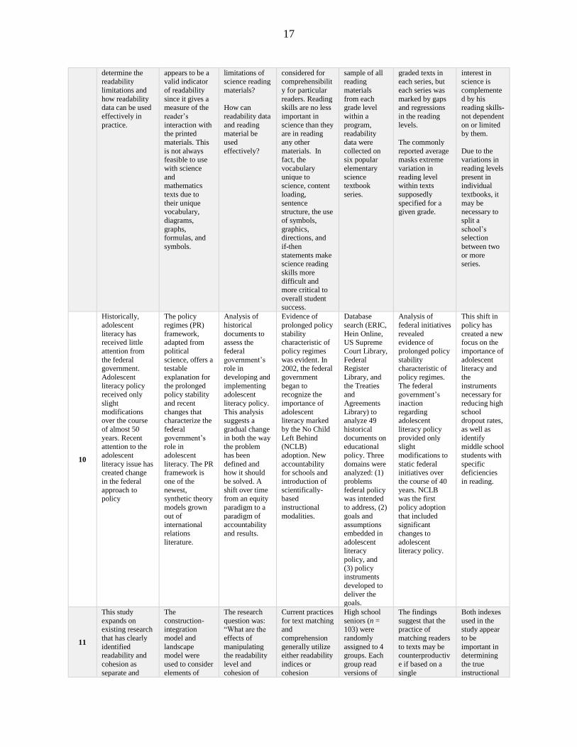
10
Historically,
adolescent
literacy has received little
attention from
the federal government.
Adolescent
literacy policy
received only
slight
modifications over the course
of almost 50
years. Recent attention to the
adolescent
literacy issue has created change
in the federal
approach to policy
The policy
regimes (PR)
framework, adapted from
political
science, offers a testable
explanation for
the prolonged
policy stability
and recent
changes that characterize the
federal
government’s role in
adolescent
literacy. The PR framework is
one of the
newest, synthetic theory
models grown
out of international
relations
literature.
Analysis of
historical
documents to assess the
federal
government’s role in
developing and
implementing
adolescent
literacy policy.
This analysis suggests a
gradual change
in both the way the problem
has been
defined and how it should
be solved. A
shift over time from an equity
paradigm to a
paradigm of accountability
and results.
Evidence of
prolonged policy
stability characteristic of
policy regimes
was evident. In 2002, the federal
government
began to
recognize the
importance of
adolescent literacy marked
by the No Child
Left Behind (NCLB)
adoption. New
accountability for schools and
introduction of
scientifically-based
instructional
modalities.
Database
search (ERIC,
Hein Online, US Supreme
Court Library,
Federal Register
Library, and
the Treaties
and
Agreements
Library) to analyze 49
historical
documents on educational
policy. Three
domains were analyzed: (1)
problems
federal policy was intended
to address, (2)
goals and assumptions
embedded in
adolescent literacy
policy, and
(3) policy instruments
developed to
deliver the goals.
Analysis of
federal initiatives
revealed evidence of
prolonged policy
stability characteristic of
policy regimes.
The federal
government’s
inaction
regarding adolescent
literacy policy
provided only slight
modifications to
static federal initiatives over
the course of 40
years. NCLB was the first
policy adoption
that included significant
changes to
adolescent literacy policy.
This shift in
policy has
created a new focus on the
importance of
adolescent literacy and
the
instruments
necessary for
reducing high
school dropout rates,
as well as
identify middle school
students with
specific deficiencies
in reading.
11
This study
expands on existing research
that has clearly
identified readability and
cohesion as
separate and
The
construction-integration
model and
landscape model were
used to consider
elements of
The research
question was: “What are the
effects of
manipulating the readability
level and
cohesion of
Current practices
for text matching and
comprehension
generally utilize either readability
indices or
cohesion
High school
seniors (n = 103) were
randomly
assigned to 4 groups. Each
group read
versions of
The findings
suggest that the practice of
matching readers
to texts may be counterproductiv
e if based on a
single
Both indexes
used in the study appear
to be
important in determining
the true
instructional

18
important
elements of text
complexity. The
focus was on quantitative
dimensions,
which are replicable across
research,
because no objective
standards exist
for defining the qualitative or
reader-task
dimensions of text complexity
cohesion as
indicators of
text complexity.
Both models conceptualize
reading
comprehension as a strategic
and cyclical
process of activating and
connecting
information within the text
and the reader’s
existing knowledge
framework.
informational
text on high
school
students’ comprehension
of causal
content in informational
texts?” The
hypothesis was comprehension
performance
will be influenced by
both
readability and cohesion such
that significant
differences
would be
apparent
between a passage at a
challenging
readability level with low
cohesion and a
passage at an easier
readability
level with high cohesion.
measures. This
study looks at
both measures of
text complexity to measure
students’
processing capacity and
strategic
formation of a coherent
representation of
the text.
the same two
informational
passages and
answered comprehensio
n test items
targeting factual recall
and inferences
of causal content.
Group A
passages had a challenging
readability
level and high cohesion;
Group B
passages had
an easier
readability
and low cohesion;
Group C
passages had a challenging
readability
level and low cohesion; and
Group D
passages had an easier
readability
and high cohesion. A 2
x 2 between-
subjects
factorial
design with
both readability
and cohesion
as independent
variables was
utilized.
quantitative
dimension.
Gauging the
complexity of a text by
readability alone
is problematic. Indexes are
based on the
notion that words of higher
frequency
occurring in shorter, simpler
sentences should
speed processing and facilitate
fluent reading,
leaving more
cognitive
resources
available for comprehending
the text.
level of text
because
students need
to be exposed to more
challenging
vocabulary and sentence
structures to
grow as readers and
be exposed to
precise content in the
subject area
domain. The causal ratio
index was
found to be
one of the
strongest
indicators of text
complexity in
a previous study
comparing
Coh-Metrix and
readability
statistics on a larger set of
passages.
Note. The study number in the first column refers to the corresponding number in Table 1.
A study was included if it addressed one or more of the focus questions (see Table 3), was
published in a peer-reviewed journal or book written by a leader in the literacy field, and was a
comparison of reading indices, it presented historical background, or addressed text
complexity/text matching issues related to readability indices.
Table 3
Key Questions for Literature Review
1. Why were readability indices developed?
2. What research methods have been used in the past to compare readability
indexed?

19
3. From the previous research, what is the treatment effect (indices comparison) on
the outcomes?
4. What effect do readability indexed have on text complexity issues?
5. What is the relationship between readability indices and text-reader matching?
History
Historically, reading assessments, and the actions that derived from such assessments, were
rooted in a political vision for eliminating poverty. Lyndon B. Johnson’s Great Society initiative
in the mid-1960s led to the Elementary and Secondary Education Act (ESEA) providing children
of low income families with provisions for education and created an unprecedented evaluation and
reporting mandate (McLaughlin, 1975). Hauptli and Cohen-Vogel (2013) examined the role of the
federal government from the Johnson-era through former President Obama and the policy shifts
around reading assessment. The following initiatives were analyzed by Hauptli and Cohen-Vogel
(2013): Economic Opportunity Act (1964), Elementary and Secondary Education Act (ESEA,
1965), Right to Read (1969), National Reading Improvement Program (education amendments to
ESEA of 1974), ESEA Education Amendments (1978), Student Literacy Corp (1988), Augustus
F. Hawkins-Robert T. Stafford Elementary and Secondary School Improvement Amendments
(1988), National Literacy Act (1991), America Reads Challenge (1996), Reading Excellence Act
(1998), National Reading Panel Report (2000), No Child Left Behind (2001), Striving Readers
Grants (2005), and Reading for Understanding (2010).
Each of these initiatives were “analyzed around adolescent literacy based on the problems
they were intended to solve, the goals they were expected to achieve and the instruments of reform,
in order to find evidence of the prolonged policy stability characteristic of policy regimes” (p.
398). Hauptli and Cohen-Vogel (2013) found federal policy rarely, if ever, focused on adolescent
(grade 4-8) literacy and “policy stasis was the overarching characterization of the federal
government’s role in adolescent literacy until a shift occurred just over a decade ago with President

20
George W. Bush extending the Clinton administration’s goal from all students reading by the end
of third grade to all students in grades 3-8 reading on grade level and establishing consequences
for schools that failed to demonstrate improvement” (p. 399). They isolated two major changes to
the regime leading up to No Child Left Behind. The first was the shift from an equity perspective
to one of accountability for schools and educators. The second, was the emergence of a power shift
in the late 1980s and 1990s from professional educators, toward state agencies and researchers.
Hauptli and Cohen-Vogel (2013) focused on the historical policies created for literacy
improvement but lacked information on assessment instruments useful for attaining positive
results.
Roller, Eller and Chapman (1980) focused on the assessment instrument utilized in the late
1960s around the time of the first federal policies for literacy improvement. The National
Assessment of Educational Progress (NAEP) was introduced to study achievement trends in
American education. The focus was solely on assessment without regard to theory or use of data
to improve outcomes.
As early as the late nineteenth century, the systematic study of text complexity in an
exclusively qualitative manner began, focusing on text features that would impact comprehension
or text readability (Pearson & Hiebert, 2014). In the early twentieth century, scientific methods
were more prevalent in solving educational problems, leading to quantitative methods for
describing text comprehensibility. Lively and Pressey (1923) proposed the first formula for
readability based on word frequency and sentence length, leading to the introduction of many other
formulas. Hiebert and Pearson (2014) found quantitative measures were disputed in research and
policy by psychologists (Gardner, 1987) whose attention focused on “understanding the roles of
particular text features in cognitive processing of information” (p. 155), and linguists (Davison &

21
Kantor, 1982) who examined consequences of lexical and syntactic changes on comprehension
and processing. However, quantitative measures were being disputed, and the digital age was
underway. Hiebert and Pearson (2014) determined “with large databanks, rankings of frequency
of words in texts could be gotten in nanoseconds” (p. 156) setting the stage for more sophisticated
analyses.
Policy
The introduction of the Common Core State Standards (2010) marked the first time a
standards document addressed the issue of text complexity. An entire standard is devoted to
increasing capacity with complex texts through a combination of qualitative, quantitative, and
reader-task analyses (Hiebert & Mesmer, 2013).
Figure 2: Common Core State Standards Model of Text Complexity
Note. From National Governors Association Center for Best Practices & Council of Chief State

22
School Officers [NGA & CCSSO]. (2010). Common Core State Standards: English Language
Arts. Washington DC: National Governors Association for Best Practices & Council of Chief State
School Officers.
CCSS claimed to be grounded in research indicating declining text complexity since the 1940s, as
noted in Appendix A of the standards:
In 2006, ACT, Inc., released a report called Reading Between the Lines that showed
which skills differentiated those students who equaled or exceeded the benchmark score
(21 out of 36) in the reading section of the ACT college admissions test from those who
did not. Prior ACT research had shown that students achieving the benchmark score or
better in reading—which only about half (51 percent) of the roughly half million test takers
in the 2004–2005 academic year had done—had a high probability (75 percent chance) of
earning a C or better in an introductory, credit-bearing course in U.S. history or psychology
(two common reading-intensive courses taken by first-year college students) and a 50
percent chance of earning a B or better in such a course.
Surprisingly, what chiefly distinguished the performance of those students who had
earned the benchmark score or better from those who had not was not their relative ability
in making inferences while reading or answering questions related to particular cognitive
processes, such as determining main ideas or determining the meaning of words and
phrases in context. Instead, the clearest differentiator was students’ ability to answer
questions associated with complex texts. Students scoring below benchmark performed no
better than chance (25 percent correct) on four-option multiple-choice questions pertaining
to passages rated as “complex” on a three-point qualitative rubric described in the report.
These findings held for male and female students, students from all racial/ethnic groups,
and students from families with widely varying incomes. The most important implication
of this study was that a pedagogy focused only on “higher-order” or “critical” thinking was
insufficient to ensure that students were ready for college and careers: what students could
read, in terms of its complexity, was at least as important as what they could do with what
they read.
The ACT report is one part of an extensive body of research attesting to the
importance of text complexity in reading achievement. The clear, alarming picture that
emerges from the evidence, briefly summarized below, is that while the reading demands
of college, workforce training programs, and citizenship have held steady or risen over the
past fifty years or so, K–12 texts have, if anything, become less demanding. This finding
is the impetus behind the Standards’ strong emphasis on increasing text complexity as a
key requirement in reading (National Governors Association Center for Best Practices &
Council of Chief State School Officers [NGA & CCSSO], 2010).
Current research, however, indicates a distinctly different pattern of historical shifts in
complexity rather than the simple declines reported by the CCSS (Gamson, Lu, & Eckert, 2013).
Gamson, Lu, and Eckert (2013) used four different measures to understand changes in text over

23
the past century; two of the measures focus on lexical difficulty (LEX and word frequency band
[WFB]) and two measures to calculate readability (Dale-Chall readability index) and Mean Length
of Sentence. Elementary textbooks published between 1905 and 2004 were analyzed, 187 third
grade texts and 71 sixth grade texts. ANOVA was used to determine significant differences in
mean between decades. The findings showed a distinctly different pattern of historical shifts in
complexity than the simple declines reported by the CCSS. The findings show a steady increase
over the past 70 years, disputing the downward trend reported by the CCSS. Text complexity is
only one dimension of a robust reading program and any efforts to unnecessarily ratchet up
complexity could cause a larger discrepancy in the achievement gap (Gamson, Lu, & Eckert,
2013). Motivation decreases when tasks become too challenging. The findings have implications
on policy, research and practice. A broader view of complexity that incorporates text, instruction,
and a wide variety of materials is needed, as well as an assessment approach using measures that
are less restrictive. Widespread mandates in policy and change in practice without stronger theory
and research is likely to have serious implications (Pearson & Hiebert, 2014). According to Hiebert
and Mesmer (2013) “when quantitative ranges are connected to a standards document adopted by
the legislatures of the vast majority of American states and the accompanying standard indicates
that students need to read from the top of a text complexity range, potential for misinterpretation
exists” (p. 46).
Readability
Begeny and Greene (2014) characterized readability as “an attribute of written text,
commonly defined by factors that theoretically make text more or less difficult to read (e.g.,
vocabulary, sentence complexity)” (p. 198). To quantify readability, mathematical formulas using
semantic and syntactic factors have been derived over the last century (Harrison, 1980).

24
Readability formulas are unique in construction; each formula consists of a combination of factors
and mathematical constants. The combination of factors and the mathematical constants used in
the different formulas can vary significantly, even when theoretically consistent (Connatser &
Peac, 1999; Harrison, 1980). Factors that are often applied to readability formulas include total
words, total sentences, total syllables, number of polysyllabic words, and words from unique
vocabulary lists. Readability formulas were originally used to determine text difficulty but have
also become a means of modifying materials to a predetermined level (Begeny & Greene, 2014).
This practice, which occurs in technical communication, research, and textbook development, can
be questionable; yet, is used commonly for text modification to obtain desired readability scores
(Connatser & Peac, 1999). Begeny and Greene (2014) stated “the widespread use of readability
estimates in education highlights the need to further investigate whether meaningful differences
exist between the grade level of the text (defined by readability formulas) and a measure of the
actual difficulty level of the text” (p. 199).
Begeny and Greene (2014) investigated readability formulas to determine which (if any)
showed an actual correspondence between grade level and difficulty level, when difficulty level is
determined by reading performance. Differing grade levels, as determined by eight commonly
used readability formulas, were examined to see whether grade levels predicted text difficulty, as
determined by oral reading fluency (ORF) scores. In the study, 360 students in second (n = 87),
third (n = 83), fourth (n = 96), and fifth (n = 94) grades in 21 different classrooms in an elementary
school located in the Southeastern United States participated. Each participant read a set of six
DIBELS (Dynamic Indicators of Basic Early Literacy) benchmark passages: two passages below
grade level, two passages at grade level, and two passages above grade level. Eight readability
estimates for each of the twelve passages were calculated using the computer software program

25
Readability Studio.
The formulas used to calculate estimates included Dale-Chall, Flesch-Kincaid, FOG,
Forcast, Fry, PSK, SMOG, and Spache. Begeny and Greene (2014) demonstrated only one (Dale-
Chall formula) of the readability formulas examined in the study was a valid measure of text
difficulty for each of its comparisons. The Dale-Chall formula successfully discriminated between
the grade level comparisons that were evaluated with the formula (i.e. third vs. fourth grade
materials and fourth vs. fifth grade materials). As one of the most commonly used formulas, the
Dale-Chall appears to be a relatively reliable formula for gauging general text difficulty across
grades 3-5 and findings are consistent with the intended purpose of the formula, to gauge text
difficulty around the fourth-grade level and above. The findings reported by Begeny and Greene
(2014) suggested most readability formulas may not assist in the selecting of text that is of greater
or lesser difficulty, whether the purpose of text selection is for instructional or assessment
purposes. Further, although findings showed that several readability formulas seem to be better at
differentiating text that is read with higher vs. lower reading abilities, nearly all formulas do not
appear to be valid indicators of text difficulty. Only reading fluency was assessed to determine
reading difficulty. The elements of comprehension and vocabulary were not considered, therefore
limiting the study outcomes. Begeny and Greene (2014) acknowledged readability formulas may
vary in appropriateness for certain grade levels due to the unique calculations of each readability
formula and the many variables that influence text difficulty.
Gallagher, Fazio, and Gunning (2012) analyzed the disparate variables that contribute to
the measures of nine readability formulas, as well as the lack of attention paid to vocabulary,
schema, and task considerations. The goal of the study was to determine how several indices
compared and whether the indices were a valid measure of various genres of science-based text.

26
The texts analyzed were science-based and selected from two Canadian publishers. Readability
levels were reported by the publishers. A total of 178 passages were chosen and tested using all
nine readability indices: (a) Gunning-Fog; (b) Flesch-Kincaid; (c) Fry; (d) Coleman-Liau; (e)
Automated Reading Index (ARI); (f) SMOG; (g) Spache; (h) Dale-Chall; and (j) Powers-Sumner-
Kearl (PSK). These indices were chosen as recognized measures used by many publishers, as well
as being a cross-section of different computational variables.
Mikk (2001) hypothesized that there should be some text characteristics that correlate with
the level of knowledge of the text content that a reader has prior to reading a text (e.g., prior
knowledge, schema). The goal was to discover text characteristics, the values of which are related
to the level of prior knowledge of the text content. Mikk (2001) analyzed 30 texts, all of a scientific
nature (e.g., physics, chemistry, astronomy, and biology). The average length of the texts was 166
words. Prior knowledge was established before subjects (n = 350) read the materials. The level of
prior knowledge was correlated with the text characteristics and 33 statistically significant
coefficients of correlation were found. A formula was calculated using regression analysis in Excel
to determine prior knowledge. The formula predicted 35% of the level of prior knowledge. Data
confirmed the hypothesis that many characteristics are related to the level of prior knowledge.
Readability formulas have some ability to predict prior knowledge and characterize the level of
familiarity and complexity of the text content and are not simply measures of linguistic
characteristics (Mikk, 2001). Although Mikk (2001) developed a formula to predict the level of
prior knowledge, the formula cannot be generalized to other populations or recommended for
practical use because the research used only popular scientific texts with a small sample of
students.
The readability of science-based texts is inextricably connected to vocabulary and

27
vocabulary is a strong predictor of text difficulty (Chall & Dale, 1995). Gallagher et al. (2012)
point out the focus on behaviorism and multidisciplinary conceptual views of reading as a means
of learning by learning theorists. The constructivist perspective has brought focus on the active
role of using experiences to build understanding of information through constructive processes to
operate, form, elaborate, and test mental structures (Driscoll, 2000).
Gallagher et al. (2012) utilized CCSS policy to focus on text complexity and increased
vocabulary demands of science-based texts. The findings of Gallagher et al. (2012) suggested due
to the complexity of discipline-specific science vocabulary, prior knowledge is required to
comprehend science texts; therefore, readability impacts instructional decision making and
appropriate strategy instruction. Curriculum and instruction have not focused on the demands of
independently reading informational text, according to the CCSS. Reading expository or
nonfiction text requires engaging prior knowledge and an understanding of specific scientific
vocabulary. According to Gallagher et al. (2012), “the linguistic features of scientific vocabulary
and the need to engage prior knowledge present challenges to the comprehension of science-based
text, therefore reading comprehension strategies (e.g., word study) should be offered to enhance
fluency” (p. 108). Reading proficiency can also be positively impacted through explicit instruction
in morphological analysis (e.g., word study). Considerable variance among the nine formulas
suggest the commonly used measures are not perfect predictors of readability. Several of the
formulas are based on high frequency word lists (e.g., Dale-Chall, Spache) which do not include
scientific words, causing an underestimation of readability levels, therefore limiting the study
outcomes. Another limitation of the Gallagher et al. (2012) study was the narrow genre of
literature. Including texts from a variety of genres and levels may produce a more accurate
outcome.

28
Shymansky and Yore (1979) noted “reading skills are no less critical in reading science
topics than they are in reading any other materials. In fact, the vocabulary peculiar to science,
content loading, sentence structure, the use of symbols, graphics, directions, and if-then
statements, make science reading skills more difficult and more critical” (p. 670). Using the Fry
Readability approach and a 10% random sample of all reading materials from each grade level
within a program and collecting readability data on six popular elementary science textbook series,
Shymansky and Yore (1979) found the average reading level was observed to progress generally
throughout the graded texts within each series, but each series was marked by gaps or regressions
in the reading levels.
The second interesting feature revealed by the analyses was that “the commonly reported
average masks extreme variation in reading levels with texts supposedly specified for a given
grade” (p. 672). Shymansky and Yore (1979) believed interest in science is complemented by
reading skills, not dependent on or limited by such skills. Science texts require strong background
knowledge to enhance understanding and one series may not fit the needs of every classroom. The
authors stated “books and reading are part of the search and organization of science knowledge
and need to be included in the science environment” (p. 676) however, science is a subject of
exploration, experimentation, and creative action and should be approached in a dynamic manner,
not as a passive activity.
Text Readability Formulas and Text Simplification
Traditional readability formulas such as Flesh Reading Ease (Flesch, 1948) have been
accepted by the educational community because they are easily associated with text simplification
(Chall & Dale, 1995). However, traditional formulas have been criticized by both first language
(L1) and second language (L2) researchers for the inability to take account of deeper levels of text

29
processing (McNamara, Kintsch, Butler-Song, & Kintsch, 1996). Several L1 validation studies
(Crossley, Greenfield, & McNamara, 2008; Crossley, Allen, & McNamara, 2011; Graesser,
McNamara, Louwerse, & & Cai, 2004; McNamara, Kintsch, Butler-Song, & Kintsch, 1996) have
found the predictive validity of traditional readability formulas to be high, correlating with
observed difficulty in the r = 0.8 range and above (Chall & Dale, 1995). Traditional readability
formulas are generally not based on theories of reading or comprehension building, but on tracing
statistical correlations (Crossley, Greenfield, & McNamara, 2008), “therefore, the credibility
accorded to them is strictly based on their demonstrated predictive power” (p. 477). The attraction
of simple, mechanical assessments has led more commonly to the use of traditional formulas for
assessing all sorts of text designed for a wider variety of reading situations, rather than for the
situations the formulas were created (Crossley, Greenfield, & McNamara, 2008).
In psycholinguistics, reading is considered a multicomponent skill operating at different
levels of processing: lexical, syntactic, semantic, and discoursal (Just & Carpenter, 1987; Koda,
2005). Reading is a skill that enables the reader to make links between features of the text and
stored representations, not only linguistic, but world knowledge, knowledge of text genre, and the
discourse model which the reader has built up of the text (Crossley, Greenfield, & McNamara,
2008). When there is more concern with comprehension, assessment must go deeper than surface
readability features to explain interactions with the text, including measures of text cohesion and
meaning construction (Gernsbacher, 1997; McNamara, Kintsch, Butler-Song, & Kintsch, 1996)
and encoding comprehension as a multilevel process (Koda, 2005). Based on the findings of
several L2 studies (Carrell, 1987; Brown, 1998) researchers determined the formulas used
generally depended on surface-level sentence difficulty indices, such as the number of words per
sentence and surface-level word difficulty indices such as syllables per words (Brown, 1998;

30
Crossley, Greenfield, & McNamara, 2008). Carrell (1987) was critical of traditional readability
formulas for not accounting for reader characteristics or for text-based factors such as syntactic
complexity, rhetorical organization, and propositional density. Brown (1998) was also concerned
that traditional readability formulas failed to account for L2 reader-based variables. In addition, it
was argued readability formulas for L2 readers needed to be sensitive to the type, function, and
frequency of words and to word redundancy within the text (Crossley, Greenfield, & McNamara,
2008).
Crossley et al. (2008) questioned whether constructing a new model incorporating at least
some variables that reflect the cognitive demands of the reading process would yield a new, more
universally applicable measure of readability. Psycholinguistic theory frames the idea that a
readability measure needs to take appropriate account of the role of working memory and the
constraints it imposes in terms of propositional density and complexity. The theoretical goal of
English readability research is to devise a measure that has strong construct validity as well as
predictive validity. Graesser, McNamara, Louwerse, and Cai (2004) reported recent advances in
numerous disciplines have made it possible to computationally investigate various measures of
text and language comprehension that supersede surface components of language and instead
explore deeper, more global attributes of language. A synthesis of the advances in these areas has
been achieved in Coh-Metrix, a computational tool that measures cohesion and text difficulty at
various levels of language, discourse, and conceptual analysis (Crossley, Greenfield, &
McNamara, 2008). The purpose of the study was to examine if certain Coh-Metrix variables can
improve the prediction of text readability, specifically the examination of variables that more
accurately reflect the cognitive processes involved in skilled L2 reading. Crossley et al. (2008)
analyzed a corpus of 32 academic reading texts to test the hypothesis that linguistic variables

31
related to cognitive processing and cohesion could better predict text readability. Mean length of
the texts was 269.28 words and mean number of sentences per hundred words was 7.10. Three
independent variables were selected to correspond to three general levels into which many
psycholinguistic accounts divide reading. These variables were lexical recognition, syntactic
parsing, and meaning construction (Just & Carpenter, 1987; Perfetti, 1985; Crossley, Greenfield,
& McNamara, 2008).
A statistical analysis of the data was conducted using R², Stein’s unbiased risk estimate
(SURE), and n-fold cross validation. Crossley et al. (2008) believed the three models were
important to analyze for the purposes of generalization. If the models were significant, by
extension, it could be argued that the readability formula would be successful in textual genres
other than academic texts. Based on the findings of the study, Crossley et al. (2008) stated the Coh-
Metrix formula has a clear superiority in accuracy to all other indices and has an “impact on
reading difficulty not of individual structures but of syntactic variety” (p. 489). The Coh-Metrix
formula allows for “a shift in perspective from considering the text to considering the reader” (p.
489). Although Crossley et al. (2008) provided a practical perspective for the L2 learner, the texts
analyzed were all from secondary textbooks and did not provide a separate or comparable set of
primary texts or genre variety. Also, the passage set was relatively small. A larger set may provide
more opportunity for generalization of findings.
As a follow-up study to Crossley et al. (2008), Crossley, Allen, and McNamara (2011)
conducted a study to examine readability formulas’ potential for evaluating a corpus of intuitively
simplified news texts (Allen, 2009). An analysis of the differences between traditional readability
formulas and readability formulas based on psycholinguistic and cognitive accounts of text
processing, i.e., the Coh-Metrix L2 Reading Index, (Crossley, Greenfield, & McNamara, 2008)

32
were analyzed to examine the potential for readability formulas to distinguish among levels of
simplified texts that have been modified using intuitive approaches in order to evaluate the
readability formulas’ construct validity and to better understand intuitive text simplification.
Crossley et al. (2011) hypothesized “the Coh-Metrix L2 Reading Index will better reflect the
intuitive text simplification processes…because such processes account for comprehension
factors, meaning construction, decoding, and syntactic parsing” (p. 85). A corpus of 300 non-
academic news texts were analyzed using Flesch-Kincaid Grade Level, Flesch Reading Ease, and
Coh-Metrix L2 indexes. Crossley et al. (2011) conducted a series of ANOVA to examine if each
readability formula demonstrated a significant difference between the levels of reading texts.
To test the accuracy of the readability formulas to distinguish between the levels of L2
reading texts, a discriminant function analysis was conducted. Cohen’s Kappa was used to measure
agreement between the actual text type and that assigned by the discriminant function analysis
model. Crossley et al. (2011) demonstrated that a readability formula based on psycholinguistic
and cognitive models of reading, and traditional readability formulas can significantly classify
texts based on levels of intuitive text simplification. However, accuracy scores were significantly
higher for the Coh-Metrix L2 Reading Index, indicating this index was better able to discriminate
between the different levels of texts. The variables used in the Coh-Metrix L2 Reading Index were
more closely aligned to the intuitive text processing for simplifying reading texts than those
provided by traditional readability formulas.
Traditional readability formulas did classify texts into appropriate categories at a level
above chance. Due to the moderate degrees of successful classifying of the Coh-Metrix, as well as
its accuracy in comparison to traditional formulas, the findings of Crossley et al. (2011) may be
extendible to genres outside academic texts. This could lead to greater accessibility for L2 learners.

33
Crossley et al. (2008) pointed out larger reading studies need to be conducted to improve the Coh-
Metrix L2 Reading Index and allow for the inclusion of additional variables and “the criteria in
such studies should include both authentic and simplified texts” (Crossley, Allen, & McNamara,
2011, p. 98). This would allow for further assessment of validity of advanced readability formulas
for predicting text comprehensibility.
Text Complexity
Text complexity remains a factor to be analyzed regarding reading comprehension and text
matching. Mesmer, Cunningham, and Hiebert (2012) defined text complexity as the elements
within the text that can be manipulated and studied. Features of complexity include the number of
unfamiliar words and sentences of greater writing sophistication (Reed & Kershaw-Herrara, 2016).
The three-part model (see Figure 2) to evaluating text complexity involves qualitative dimensions
(e.g., levels of meaning, schema), reader and task considerations (e.g., motivation, knowledge,
experiences, and purpose of the assignment) and quantitative dimensions (e.g., readability and
cohesion).
The first two dimensions are described as requiring informed decisions regarding the reader
(Hiebert & Mesmer, 2013), however, both lack extant research on the reliability or validity of such
decision-making processes or the resulting designations of text (Reed & Kershaw-Herrara, 2016).
Quantitative measures such as readability have had declining visibility in education research in the
past 20 years (Wray & Janan, 2013). Wray and Janan (2013) recognized the CCSS has had a global
effect on text complexity. Reading instruction needs to take place at all levels and in all content
areas. It was determined that the process of reading has moved from describing a process of gaining
meaning from a text to one of creating meaning through interaction with a text. The implications
of the study indicated deliberate policies and strategies are needed to highlight the importance of

34
increasingly complex texts. Wray and Janan (2013) focused on all three dimensions of readability
as they relate to text complexity yet failed to provide a solution to the problem most prevalent in
relation to reading, namely comprehension and motivation.
Reed and Kershaw-Herrara (2016) conducted a study to examine the role of quantitative
dimensions of text complexity and the effects of these dimensions on comprehension. High school
seniors (n = 103) were randomly assigned to 4 groups. Each group read versions of the same two
informational passages and answered comprehension test items targeting factual recall and
inferences of causal content. Group A passages had a challenging readability level and high
cohesion; Group B passages had an easier readability and low cohesion; Group C passages had a
challenging readability level and low cohesion; and Group D passages had an easier readability
and high cohesion. A 2 x 2 between-subjects factorial design with both readability and cohesion
as independent variables was utilized.
The hypothesis of the study was “comprehension performance would be influenced by both
readability and cohesion such that significant differences would be apparent between a passage at
a challenging level with low cohesion and a passage at an easier readability level with high
cohesion” (p. 79). No significant differences in prior comprehension abilities or prior knowledge
of passage content were found based on a one-way analysis of variance (ANOVA). Readability
level had a moderate effect on comprehension when passages had low cohesion. This was
consistent with research that analyzed the dynamic elements of reader, text, and activity (Snow &
Sweet, 2003). The findings of Reed and Kershaw-Herrara (2016) lend further support to the idea
that text matching may be counterproductive if based on a single quantitative dimension (Hiebert
& Mesmer, 2013; National Governors Association Center for Best Practices & Council of Chief
State School Officers [NGA & CCSSO], 2010). Although current recommendations are to use a

35
multifaceted approach to evaluating text complexity, available concrete guidance is limited to
suggesting how readability be interpreted, used and incorporated into the instructional decision-
making process (Begeny & Greene, 2014; Mesmer, Cunningham, & Hiebert, 2012; National
Governors Association Center for Best Practices & Council of Chief State School Officers [NGA
& CCSSO], 2010; Reed & Kershaw-Herrara, 2016). Deep comprehension requires an integration
of new information with prior knowledge (Guthrie, et al., 2006; Just & Carpenter, 1987; Shanahan,
Fisher, & Fray, 2012). This study was limited to informational passages with similar organizational
structures, thus it could not be generalized to other types of reading passages. However, the
findings did suggest that gauging the complexity of a passage by readability alone is problematic,
thus suggesting a need for analysis of cohesion.

36
CHAPTER 3 Methodology
Design and Sample
An analysis of narrative and expository texts deemed appropriate for grades 1-5 by the
publisher, as well as a leveling system created by Fountas and Pinnell (2001), will be compared
using readability indices. The target population will be all narrative and expository texts at a grade
1-5 reading level and the accessible population will be those texts that are available within local
schools, libraries, and private collections. Non-probability sampling will be used to identify a
convenience sample of 30 narrative and 30 expository texts at each grade level, taken from a local
elementary guided reading collection, local libraries, and personal collection of texts.
The total sample size will be N = 300. A 100-word passage from each text will be arbitrarily
selected. Each passage will be analyzed using the following eight readability indexes: Flesch-
Kincaid Grade Level index (Flesch, 1948), Flesch Reading Ease formula (Flesch, 1951), Fry
Readability graph (Fry, 1968; Fry, 1975), Dale-Chall Readability formula (Dale & Chall, 1948),
Spache Readability formula (Spache, 1953), Gunning Fog index (Gunning, 1968), the SMOG
Grading Plan (McLaughlin, 1969) and the Coh-Metrix L2 index (Graesser, McNamara, Louwerse,
& Zhiquiang, 2004). These formulas represent a cross-section of different computational variables
including: number of sentences, syllables, number of characters, multi-syllabic words, and
vocabulary complexity (Gallagher, Fazio, & Gunning, 2012). Table 4 provides the formulas used
to calculate each of the readability indices used in this study.
Table 4
Computational Formulas for Reading Indexed
Formulas Mathematical Computation Notes
Flesch-Kincaid 0.39 x (W/S) + 11.8 x (SY/W) – 15.59
S-total sentences
SY-total syllables
W-total words

37
Flesch Reading
Ease
206.835 – (1.015 x W/S) – (84.600 x
SY/W)
S-total sentences
SY-total syllables
W-total words
Fry
Count the number of sentences and the
number of syllables in a 100-word passage.
Plot a dot on the Fry Readability Graph
where the two variables intersect. The area
where the dot is plotted signifies the
approximate reading grade level.
Dale-Chall (W/S x 0.0496) + (DW/W x 100 x 0.1579)
+ 3.6365
DW-total difficult words
(based on the 3000 Dale-
Chall word list)
S-total sentences
W-total words
Spache (0.141 x (W/S)) + (0.086 x (UDW/W) x
100) + 0.839
S-total sentences
UDW-total unique difficult
words not in the Spache
Word List
W-total words
Gunning-Fog 0.4 x ((W/S) + (PSY/W x 100))
PSY-total polysyllabic
words (words with 3 or
more syllables)
S-total sentences
W-total words
SMOG 3.1291 + (1.043 x ˰√(𝑃𝑆𝑌
𝑆∗ 30) )
PSY-total polysyllabic
words (words with 3 or
more syllables)
S-total sentences
Coh-Metrix L2 -45.032 + (52.230 x CWO) + (61.306 x
SSS) + (22.205 x CELEX)
CWO-content word overlap
SSS-sentence syntax
similarities
CELEX-word frequency
index
Note. Adapted from “Varying Readability of Science-Based Text in Elementary Readers:
Challenges for Teachers,” by T. L. Gallagher, X. Fazio, and T. G. Gunning, 2012, Reading
Improvement, pg. 112.
The Bland-Altman method will use the data gathered from each of the readability indices to
determine agreement between each of the indices.

38
Agreement and Bland-Altman Method
Correlation and hypothesis testing are often used methods for determining agreement
between two measures (e.g., Pearson Product-Moment coefficient, linear regression, multiple
regression, discriminant function analysis, and t – tests). An established method to quantify
agreement between two quantitative measurements by constructing limits of agreement was
developed by Altman and Bland (1983; see also Giavarina, 2015).
The original goal was to detect bias, either fixed or proportional, between methods.
Ludbrook (2010) stated “fixed bias means that one set of measurements gives values that are
consistently higher (or lower) than the other, across the whole range of measurement (p. 144). The
parameters α and β quantify the bias of the measurement system relative to the reference system.
The fixed bias is referred to as α since it increases or decreases the average measurement of the
second system by a fixed amount, and β refers to the proportional bias because it biases the second
system’s measurements by an amount that is proportional to the true values (Stevens, Steiner, &
MacKay, 2015). This method was not meant to calibrate one method against another therefore, it
does not indicate an advantage of applying one method over another. The two methods do not need
to be identical to be used interchangeably if they provide similar measurements, in other words,
the systems agree. Moen (2016) stated the population from which the two measures are drawn
should not be an issue for determining agreement unless there is a problem (bias or instrument
imprecision) with the measurement devices. This method has most commonly been used in the
fields of medicine and science.
The limits of agreement approach characterizes the agreement between two measurement
systems by evaluating the difference between measurements made on the same subject (Stevens,
Steiner, & MacKay, 2015). The limits of agreement are calculated using the mean and the standard

39
deviation (s) of the difference between two measurements. To check the assumption of normality
of differences and other characteristics, a graphical representation is used (Giavarina, 2015). The
resulting graph is a scatterplot XY, in which the Y-axis expresses the difference between the two
paired measurements (A – B) and the X-axis shows the average of the measures ((A + B) / 2).
Figure 3: Sample Bland-Altman Plot
Note. Adapted from PubMed Central. Retrieved October 9, 2017 from
https://www.ncbi.nlm.nih.gov/pmc/articles/PMC4470095/bin/bm-25-141-f2.jpg
Bland and Altman (1983) recommended that 95% of the data points should lie within ±2s of the
mean difference, if the differences are normally distributed (Gaussian).
The Bland-Altman plot represents every difference between two paired methods against
the average of the measurement and plotting difference against mean allows for investigating any
possible relationship between measurement error and the true value (Giavarina, 2015). The limits
of agreement will shift with each new sample added to the analysis (Altman & Bland, 1983),
therefore, implications derived from a Bland-Altman plot are subjective, which could lead to error

40
in the conclusion that interchangeability exists where a statistical test may demonstrate that it does
not (Moen, 2016). It is suggested by Stevens et al. (2015) to check the assumptions of normal
distribution and that the repeatability is constant across the range of true values by using a QQ-
plot and a repeatability plot. Non-parametric tests of distribution, such as Shapiro-Wilks or
Kolmogorov-Smirnov test, can also be used to determine normal distribution of the sample
(Giavarina, 2015). It is also suggested by Giavarina (2015) that the best way to use the Bland-
Altman plot would be “to define a priori the limits of maximum acceptable differences, or the
limits of agreement expected based on analytically relevant criteria, and then to obtain the statistics
to see if these limits are exceeded, or not” (p. 146).
Reliability of Readability Indices
Reliability has been widely examined throughout the history of readability indices.
Readability measurement is a research tradition that dates back to the beginning of the 20th century
when the formulas produced purported to estimate the relative difficulty of a passage by a
combination of factors (Stahl, 2003). Readability formulae are rough guides of text difficulty, with
most having large standard errors of measurement of a full grade level or more (Chall & Dale,
1995; Zakaluk & Samuels, 1988).
Hintze and Christ (2004) reported that readability estimates could be used to control for
passage readability which resulted in significantly smaller measurement of errors (i.e., lower
standard error and standard error of estimates). The attraction of simple, mechanical assessments
has led to the common use of readability indexes for assessing a wide variety of texts, readers, and
reading situations beyond those for which the formulas were created (Crossley, Allen, &
McNamara, 2011). Traditional readability formulas are simple algorithms that measure text
readability based on sentence length and word length and have been found to successfully predict

41
first language (L1) text readability (Crossley, Allen, & McNamara, 2011). However, discourse
analysts (Davison & Kantor, 1982) have widely criticized readability indices as being weak
indicators of comprehensibility and for not closely aligning with the cognitive processes involved
in text comprehension (Crossley, Allen, & McNamara, 2011). A lack of reliability has been noted
by others, such as Crossley et al. (2008) who contend that formula variables relating to cognitive
reading processes (e.g. decoding, syntax, meaning) contribute significantly to better readability
measures than the surface variables used in traditional formulas. Similarly, Bailin and Grafstein
(2001) stated traditional readability indices fall short on considering elements such as grammar,
style, background knowledge, and textual characteristics. The variances among different indices
indicates that they are not perfect predictors of readability estimates; however, they offer
probability statements and estimates of text difficulty (Gallagher, Fazio, & Gunning, 2012). The
notion that no formula yields an exact readability level has been supported by Fitzgerald (1980)
who reported great variation in formula scores due to sampling methods. Formulas may yield
unreliable estimates from small numbers of samples and generally are reliable only when the
samples include the entire text using continuous 100-word passages from the beginning to the end
of the text (Rush, 1985).
Reliability lies within the consistency of the readability index to measure the constructs it
purports to measure. As such, a readability index that demonstrates adequate reliability with one
sample (i.e. text passage) may not demonstrate the same reliability with a different sample due to
the variable text features. Reliability also varies from one readability index to all other indexes.
For example, Ricker (1978) reported the Fry index and the SMOG formula produced readability
levels that appear to be almost two grade levels apart; the SMOG formula yielded scores two grade
levels higher than the Fry index. Therefore, caution needs to be used in accepting average
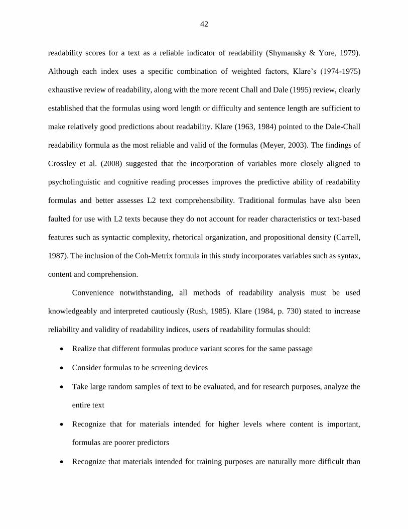
42
readability scores for a text as a reliable indicator of readability (Shymansky & Yore, 1979).
Although each index uses a specific combination of weighted factors, Klare’s (1974-1975)
exhaustive review of readability, along with the more recent Chall and Dale (1995) review, clearly
established that the formulas using word length or difficulty and sentence length are sufficient to
make relatively good predictions about readability. Klare (1963, 1984) pointed to the Dale-Chall
readability formula as the most reliable and valid of the formulas (Meyer, 2003). The findings of
Crossley et al. (2008) suggested that the incorporation of variables more closely aligned to
psycholinguistic and cognitive reading processes improves the predictive ability of readability
formulas and better assesses L2 text comprehensibility. Traditional formulas have also been
faulted for use with L2 texts because they do not account for reader characteristics or text-based
features such as syntactic complexity, rhetorical organization, and propositional density (Carrell,
1987). The inclusion of the Coh-Metrix formula in this study incorporates variables such as syntax,
content and comprehension.
Convenience notwithstanding, all methods of readability analysis must be used
knowledgeably and interpreted cautiously (Rush, 1985). Klare (1984, p. 730) stated to increase
reliability and validity of readability indices, users of readability formulas should:
• Realize that different formulas produce variant scores for the same passage
• Consider formulas to be screening devices
• Take large random samples of text to be evaluated, and for research purposes, analyze the
entire text
• Recognize that for materials intended for higher levels where content is important,
formulas are poorer predictors
• Recognize that materials intended for training purposes are naturally more difficult than

43
other kinds of texts
• Consider the effects of motivation and prior knowledge on comprehension
• Not rely on formulas alone but include expert judges
• Not use formulas as part of writing
Data Analysis
All reading passages will be manually typed or scanned into Microsoft Word for analysis.
Passages that are manually typed will be proofread by a third party. Scanned passages will be
proofread by the author. The texts will be entered into two websites capable of computing the eight
readability indexes. The Readability Formulas website (www.readabilityformulas.com) calculates
seven measures of readability including the following indices: Flesch-Kincaid Grade Level, Flesch
Reading Ease, Fry Readability graph, Dale-Chall, Spache, Gunning-Fog, and SMOG. The Coh-
Metrix website (www.cohmetrix.com) calculates three measures of readability including the
following indices: Flesch-Kincaid Grade Level, Flesh Reading Ease, and Coh-Metrix L2. These
websites were vetted by comparing sample results from each site, particularly Flesch-Kincaid
Grade Level and Flesh Reading Ease because both sites compute these indexes. Also, the formulas
used to compute each readability index on the Readability Formulas site and Coh-Metrix site were
compared to the formulas listed in Table 4 and found to be identical. Each passage will be analyzed
with all eight readability indices to produce a score; or reading level. It is important to qualify that
indexes recommended for use with text at a Grade 3 level or lower (i.e. Spache) and indexes
recommended for use with text at a Grade 4 level or higher (i.e. Dale-Chall, SMOG) will be used
with all levels of text.
Descriptive statistics (i.e. mean, standard deviation) on all data will be calculated using
Microsoft Excel. These statistics will be used to determine agreement between each comparison

44
set (see Table 5) as required by the Bland-Altman method. A Bland-Altman plot will be created
for each pair of quantitative measures to assess interchangeability of readability indices. A
maximum acceptable difference for each readability index comparison will be one and one-half
(1.5) grade levels, as determined through the calculated limits of agreement. Microsoft Excel will
be used to calculate individual plot points and to create a Bland-Altman plot for each comparison
set. A total of 28 plots will be created and analyzed.
Table 5
Paired Readability Indices to Determine Agreement Using Bland-Altman Plots
Readability Index Groupings
1. Flesch-Kincaid Grade Level and Flesch Reading Ease
2. Flesch-Kincaid Grade Level and Dale-Chall
3. Flesch-Kincaid Grade Level and Gunning Fog
4. Flesch-Kincaid Grade Level and SMOG
5. Flesch-Kincaid Grade Level and Fry Readability Graph
6. Flesch-Kincaid Grade Level and Spache
7. Flesch-Kincaid Grade Level and Coh-Metrix L2
8. Flesch Reading Ease and Dale-Chall
9. Flesch Reading Ease and Gunning Fog
10. Flesch Reading Ease and SMOG
11. Flesch Reading Ease and Fry Readability Graph
12. Flesch Reading Ease and Spache
13. Flesch Reading Ease and Coh-Metrix L2
14. Dale-Chall and Gunning Fog
15. Dale-Chall and SMOG

45
16. Dale-Chall and Fry Readability Graph
17. Dale-Chall and Spache
18. Dale-Chall and Coh-Metrix L2
19. Gunning Fog and SMOG
20. Gunning Fog and Fry Readability Graph
21. Gunning Fog and Spache
22. Gunning Fog and Coh-Metrix L2
23. SMOG and Fry Readability Graph
24. SMOG and Spache
25. SMOG and Coh-Metrix L2
26. Fry Readability Graph and Spache
27. Fry Readability Graph and Coh-Metrix L2
28. Spache and Coh-Metrix L2

46
CHAPTER 4 Results
Unintended Findings
A total of 300 reading passages were typed into Microsoft Word for analysis using eight
readability indexes. Each reading passage was proofread by two readers. The first proofreading
was completed by the researcher and the second proofreading was completed by an independent
reader. The passages were then analyzed using www.readabilityformulas.com and
www.cohmetrix.com. Each passage received eight individual scores; one for each readability
index. Bland-Altman plots were created in Microsoft Excel for each of the twenty-eight (28)
comparison sets found in Table 5. During the course of the analyses, it was determined that two of
the readability indexes did not measure the same constructs as the other six. Therefore, it was
necessary to eliminate Flesch Reading Ease and Coh-Metrix for this study resulting in fifteen (15)
comparison sets instead of twenty-eight (28). Also, it was determined that several of the reading
passages created outliers that skewed the data. Those reading passages were eliminated from the
analyses for accuracy. The remaining readability indexes included Flesch-Kincaid Grade Level,
Fry Readability Graph, Dale-Chall, Spache, Gunning Fog, and Smog. Table 6 shows the sample
sizes for each grade level and genre that were used in the data analyses after removing the outliers
that did not fit into the Grade 1-5 sampling. A total of 244 reading passages were used in the final
analyses.
Analysis
Fifteen comparisons were analyzed using Bland-Altman plots, percentage error and
correlation. The comparisons were: Flesch-Kincaid Grade Level-Fry Graph, Flesch-Kincaid Grade
Level-Dale-Chall, Flesch-Kincaid Grade Level-Spache, Flesch-Kincaid Grade Level-Gunning
Fog, Flesch-Kincaid Grade Level-Smog, Fry Graph-Dale-Chall, Fry Graph-Spache, Fry Graph-

47
Gunning Fog, Fry Graph-Smog, Dale-Chall-Spache, Dale-Chall-Gunning Fog, Dale-Chall-Smog,
Spache-Gunning Fog, Spache-Smog, and Gunning Fog-Smog. The difference was calculated for
each pair and analyzed for normality in IBM SPSS Statistics 25 using the Shapiro-Wilk test and
QQ plots. Raw data found to be normal were utilized to calculate mean and difference for each of
the data points in the analysis. When the raw data were found to be heteroscedastic, instead of
computing the difference between the data points, the ratio of the data sets were computed and
used for the Bland-Altman plot, as noted in Bland and Altman (1999, pg. 145).
Table 6
Reading Passage Sample Sizes
Grade Fiction (n) Non-Fiction (n)
1 29 18
2 30 30
3 26 34
4 18 29
5 13 17
Total (n) 116 128
Bias and standard deviation were calculated from the mean and difference, or ratio. These
statistics were then used to calculate the limits of agreement (LoA), both upper and lower. The
spread of the LoA was calculated by finding the difference between the upper and lower limits of
agreement. When proportional error was evident in the Bland-Altman plot, the percentage error
was calculated. The percentage error is the proportion between the magnitude of measurement
and the error in measurement (Hanneman, 2008). Hanneman (2008) indicated the Bland-Altman
plot allows for visualization of proportional error but due to bias and repeatability estimates

48
being computed across all data points, the proportional error may not be visible in the estimate,
however calculating the percentage error remedies the issue. The percentage error was calculated
by dividing the spread of the limits of agreement by the average for the measurements obtained
by the established method.
The correlation coefficient was calculated in Microsoft Excel to determine if a predictable
relationship exists between two instruments that purport to measure estimated grade level. The
readability comparison sets that were found to have high correlation were:
• Flesch-Kincaid Grade Level vs. Fry Graph (Fiction, r = .902; Non-Fiction, r = .885)
• Flesch-Kincaid Grade Level vs. Spache (Fiction, r = .740; Non-Fiction, r = .600)
• Flesch-Kincaid Grade Level vs. Gunning Fog (Fiction, r = .857; Non-Fiction, r = .823)
• Flesch-Kincaid Grade Level vs. Smog (Fiction, r = .712; Non-Fiction, r = .776)
• Fry Graph vs. Gunning Fog (Fiction, r = .860; Non-Fiction, r = .783)
• Fry Graph vs. Smog (Fiction, r = .659, Non-Fiction, r = .727)
• Gunning Fog vs. Smog (Fiction, r = .708; Non-Fiction, r = .905)
For each comparison of data sets, it was determined that a sampling of grade level and
genre would be used to evaluate interchangeability with Bland-Altman plots. Not all grade levels
of fiction and non-fiction were analyzed. Three grade levels/genres were randomly selected for
each comparison. Each of the Bland-Altman plots broken out by grade and genre are included in
Appendix A. Although agreement was ultimately determined based on the preceding sampling, an
analysis of each comparison set by genre including all grades 1-5 was also conducted and Bland-
Altman plots were constructed. These plots are included in Appendix B.
Spache vs. Gunning Fog
The first data set comparison assessed the agreement between Spache and Gunning Fog.

49
Five data sets were analyzed for this comparison: Fiction-all five (5) grade levels, Non-Fiction-all
five (5) grade levels, Fiction-Grade 3, Non-Fiction-Grade 2, and Non-Fiction Grade 4. Table 7
includes a breakdown of each comparison.
All comparison sets were found to have a normally-distributed set of differences based on
the Shapiro-Wilk test, allowing for analysis of the raw data. No ratio transformations were
performed.
The bias also represents the average difference between the two measures. The maximum
difference set a priori was one and one-half grade levels (1.5). The comparisons that fall within
this measure and appear to have agreement are Fiction Grade 1-5 and Non-Fiction Grade 2. Non-
Fiction Grade 2 has a relatively small correlation coefficient of r = .147 and a large percentage
error of 0.97. Although the larger sample size of the Fiction Grade 1-5 (n = 116) appears to effect
agreement, it is not validated by the Non-Fiction Grade 1-5 comparison which has an even larger
sample size (n = 128). There appears to be agreement between Spache and Gunning Fog readability
indexes when the sample size is large, and the text genre is fiction.
Table 7
Spache vs. Gunning Fog
Fiction
Grade 1-
5
Non-Fiction
Grade 1-5
Fiction
Grade 3
Non-Fiction
Grade 2
Non-Fiction
Grade 4
Mean (Bias) -1.36293 -1.91172 -1.56154 -1.14 -2.8069
SD 1.13846 1.396769 0.936836 0.85242 1.322857
Upper LOA 0.868451 0.825949 0.27466 0.530744 -0.2141
Lower LOA -3.59341 -4.64939 -3.39774 -2.81074 -5.3997
Spread LOA 4.4628 5.4753 3.672 3.3415 5.1856

50
Percentage
error
n/a* n/a* 0.934 0.97 n/a*
Correlation 0.63 0.38 -0.127 0.147 -0.34
*Note: percentage error not appropriate possibly due to extreme outliers
Figures 4-8 contain the Bland-Altman plots for each of the Spache-Gunning Fog
comparisons.
Figure 4. Fiction Grade 1-5 Spache-Gunning Fog Bland-Altman Plot
Figure 5. Non-Fiction Grade 1-5 Spache-Gunning Fog Bland-Altman Plot
-5
-4
-3
-2
-1
0
1
2
3
0 1 2 3 4 5 6 7 8
Fiction Spache vs. Gunning Fog
-8
-6
-4
-2
0
2
4
0 1 2 3 4 5 6 7 8 9
Non-Fiction Spache vs. Gunning Fog
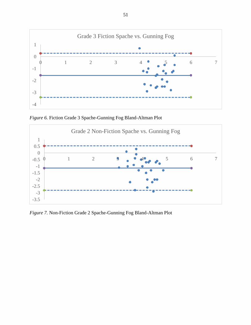
51
Figure 6. Fiction Grade 3 Spache-Gunning Fog Bland-Altman Plot
Figure 7. Non-Fiction Grade 2 Spache-Gunning Fog Bland-Altman Plot
-4
-3
-2
-1
0
1
0 1 2 3 4 5 6 7
Grade 3 Fiction Spache vs. Gunning Fog
-3.5
-3
-2.5
-2
-1.5
-1
-0.5
0
0.5
1
0 1 2 3 4 5 6 7
Grade 2 Non-Fiction Spache vs. Gunning Fog

52
Figure 8. Non-Fiction Grade 4 Spache-Gunning Fog Bland-Altman Plot
Each of the five (5) Bland-Altman plots have been included for the first comparison. The following
comparisons will utilize the breakouts of grade level/genre and include only those plots that are
significant to the analysis. The plots including Grades 1-5 Fiction and Non-Fiction for each
comparison are included in Appendix B.
Flesch-Kincaid Grade Level vs. Fry Graph
The three (3) breakout data sets used to assess agreement for Flesch-Kincaid Grade Level
and Fry Graph were Fiction Grade 1, Fiction Grade 2, and Non-Fiction Grade 3. The data for
Fiction Grade 2 and Non-Fiction Grade 3 were normally distributed. Therefore, the raw data were
used to create Bland-Altman plots. Fiction Grade 1 data, however, were non-normal. A ratio
transformation was performed on this set of data. The ratio data were used to create the Bland-
Altman plot. Table 8 includes a breakdown of each of the three (3) comparisons.
The difference of each set falls within the allowed 1.5 grade levels, suggesting possible
agreement. Each Bland-Altman plot reveals an interesting pattern. As the average increases in each
set, the difference decreases in a linear fashion. The linear sets of data do not suggest a relationship
between differences and averages, as would be expected when two measures agree. When two
-6
-5
-4
-3
-2
-1
0
0 1 2 3 4 5 6 7 8
Grade 4 Non-Fiction Spache vs. Gunning Fog

53
measures agree the scatter of data points will fall near the bias line. There appears to be
proportional bias between these two measures. A large measure of proportional error was detected
in the Non-Fiction Grade 4 data set. The spread of each LoA also appears to be wider than desired
when evaluating for agreement.
Table 8
Flesch-Kincaid Grade Level vs. Fry Graph
Fiction Grade 1 (ratio) Fiction Grade 2 Non-Fiction Grade 4
Mean (Bias) 0.906897 -0.016667 -1.23235
SD 0.351288 0.806475 0.780344
Upper LOA 1.595421 1.564025 0.297102
Lower LOA 0.218372 -1.597358 -2.76181
Spread LOA 1.377048 3.161383 3.05891
Percentage error n/a* n/a* 0.88
Correlation 0.47859 0.462697 0.47134
*Note: percentage error not appropriate possibly due to extreme outliers
The Bland-Altman plots for these comparisons are included in Figures 9-11. The linear patterns
are apparent among all data sets when Fry Graph is analyzed. There does not appear to be
agreement between Flesch-Kincaid Grade Level and Fry Graph readability indexes based on the
data and the plots.

54
Figure 9. Fiction Grade 1 Flesch-Kincaid Grade Level-Fry Graph Bland-Altman Plot
Figure 10. Fiction Grade 2 Flesch-Kincaid Grade Level-Fry Graph Bland-Altman Plot
0
0.5
1
1.5
2
0 0.5 1 1.5 2 2.5 3 3.5
Grade 1 Fiction (Ratio) Flesch Kincaid GL vs. Fry Graph
-2
-1.5
-1
-0.5
0
0.5
1
1.5
2
0 0.5 1 1.5 2 2.5 3 3.5 4
Grade 2 Fiction Flesch-Kincaid GL vs. Fry Graph

55
Figure 11. Non-Fiction Grade 3 Flesch-Kincaid Grade Level-Fry Graph Bland-Altman Plot
Flesch-Kincaid Grade Level vs. Dale-Chall
The three (3) breakout data sets used to assess agreement for Flesch-Kincaid Grade Level
and Dale-Chall were Fiction Grade 3, Non-Fiction Grade 4, and Non-Fiction Grade 5. The Non-
Fiction Grade 4 and Non-Fiction Grade 5 sets provided normally distributed data, therefore, the
raw data were used to construct these Bland-Altman plots. Fiction Grade 3 however provided non-
normal distribution of data. Ratio transformations were performed on this set of data. The ratio
data were used to create the Bland-Altman plot. Table 9 includes a breakdown of each of the three
(3) comparisons.
Table 9
Flesch-Kincaid Grade Level vs. Dale-Chall
Fiction Grade 3 (Ratio) Non-Fiction Grade 4 Non-Fiction Grade 5
Mean (Bias) 0.697883 -1.267857 -1.07647
SD 0.626022 0.697643 0.559609
Upper LOA 1.924887 0.099524 0.020362
Lower LOA -0.52912 -2.635238 -2.1733
-3.5
-3
-2.5
-2
-1.5
-1
-0.5
0
0.5
0 1 2 3 4 5 6 7
Grade 3 Non-Fiction Flesch-Kincaid GL vs. Fry Graph

56
Spread LOA 2.454007 2.734762 2.19366
Percentage error 0.71210 0.60967 0.41116
Correlation 0.29046 -0.10940 0.33099
The difference of each set falls within the allowed 1.5 grade levels suggesting possible
agreement. Fiction Grade 3 provides a Bland-Altman plot that also suggests agreement based on
the cluster of data around the bias line. Figure 12 provides the Bland-Altman plot of Fiction Grade
3. Although there appears to be a large percentage error for this data set, one extreme outlier
apparently skews the findings. Although other factors may be influencing the outcome of this data,
the comparison set suggests agreement between Flesch-Kincaid Grade Level and Dale-Chall
readability indexes, especially when analyzing Fiction Grade 3 material.
Figure 12. Fiction Grade 3 Flesch-Kincaid Grade Level-Dale-Chall Bland-Altman Plot
Non-Fiction Grade 4 and Non-Fiction Grade 5 produce Bland-Altman plots similar in
shape and distribution. These plots are provided in Figure 13 and Figure 14.
-1
0
1
2
3
4
0 1 2 3 4 5 6 7
Grade 3 Fiction Flesch-Kincaid GL (Ratio) vs. Dale-Chall

57
Figure 13. Non-Fiction Grade 4 Flesch-Kincaid Grade Level-Dale-Chall Bland-Altman Plot
Sample size (n = 17) for Grade 5 Non-Fiction Flesch-Kincaid Grade Level vs. Dale-Chall
limits the outcome of the data. However, the majority of the data points fall within the limits of
agreement. The full Non-Fiction Grades 1-5 plot supports the suggestion of agreement between
these two measures. Although there appear to be several outliers, the majority of the data points
cluster around the bias line and provide a larger sample size (n = 129). See Appendix B for the
Bland-Altman plot.
Figure 14. Non-Fiction Grade 5 Flesch-Kincaid Grade Level-Dale-Chall Bland-Altman Plot
Flesch-Kincaid Grade Level vs. Spache
-3.5
-3
-2.5
-2
-1.5
-1
-0.5
0
0.5
0 1 2 3 4 5 6 7
Grade 4 Non-Fiction Flesch-Kincaid GL vs. Dale-Chall
-3
-2.5
-2
-1.5
-1
-0.5
0
0.5
0 1 2 3 4 5 6 7 8 9
Grade 5 Non-Fiction Flesch-Kincaid GL vs. Dale-Chall

58
The three (3) breakout data sets used to assess agreement for Flesch-Kincaid Grade Level
and Spache were Fiction Grade 1, Fiction Grade 5, and Non-Fiction Grade 4. The Non-Fiction
Grade 4 set provided normally distributed data, therefore, the raw data were used to construct the
Bland-Altman plot. Fiction Grade 1 and the Fiction Grade 5, however, provided non-normal
distribution of data. Ratio transformations were performed on these sets of data. The ratio data
were used to create the Bland-Altman plots. Table 10 includes a breakdown of each of the three
(3) comparisons.
The difference of each set falls within the allowed 1.5 grade levels suggesting possible
agreement. Each of the fiction data sets has little proportional error and the data points fall within
the limits of agreement, clustered loosely around the bias line. Fiction Grade 1 and Fiction Grade
5 also have a small spread of limits of agreement further suggesting agreement may be possible.
Figures 15-16 provide the Bland-Altman plots for Fiction Grade 1 and Fiction Grade 5.
Table 10
Flesch-Kincaid Grade Level vs. Spache
Fiction Grade 1
(Ratio)
Fiction Grade 5
(Ratio)
Non-Fiction Grade
4
Mean (Bias) 0.471245 1.240932 0.586207
SD 0.105412 0.119818 0.631169
Upper LOA 0.677853 1.475774 1.823298
Lower LOA 0.264637 1.006089 -0.65088
Spread LOA 0.413216 0.469685 2.474183
Percentage
error
0.1946 0.086 0.4070
Correlation 0.5388 0.0827 0.108

59
Figure 15. Fiction Grade 1 Flesch-Kincaid Grade Level-Spache Bland-Altman Plot
Figure 16. Fiction Grade 5 Flesch-Kincaid Grade Level-Spache Bland-Altman Plot
The data are less strong when analyzing Non-Fiction Grade 4. There appears to still be agreement
based on the difference, however, the spread of the limits of agreement is much larger and the
proportional error that exists is greater. Sample size (n = 29) is the same as Fiction Grade 1 (n =
29) but greater than Fiction Grade 5 (n = 13). Figure 17 provides the Bland-Altman plot for Non-
Fiction Grade 4. The Bland-Altman plot for Fiction Grades 1-5 also suggests agreement based on
the difference and a narrow spread of limits of agreement. See Appendix B for the plot.
0
0.1
0.2
0.3
0.4
0.5
0.6
0.7
0.8
0 0.5 1 1.5 2 2.5 3 3.5 4
Grade 1 Fiction (Ratio) Flesch-Kincaid GL vs. Spache
0
0.2
0.4
0.6
0.8
1
1.2
1.4
1.6
0 1 2 3 4 5 6 7
Grade 5 Fiction (Ratio) Flesch-Kincaid GL vs. Spache

60
Figure 17. Non-Fiction Grade 4 Flesch-Kincaid Grade Level-Spache Bland-Altman Plot
Flesch-Kincaid Grade Level vs. Gunning Fog
The three (3) breakout data sets used to assess agreement for Flesch-Kincaid Grade Level
and Gunning Fog were Fiction Grade 3, Fiction Grade 5, and Non-Fiction Grade 3. The Fiction
Grade 3 and Non-Fiction Grade 3 sets provided normally distributed data, therefore, the raw data
were used to construct the Bland-Altman plots. The Fiction Grade 5, however, provided non-
normal distribution of data. Ratio transformations were performed on this set of data. The ratio
data were used to create the Bland-Altman plot. Table 11 includes a breakdown of each of the
three (3) comparisons.
Table 11
Flesch-Kincaid Grade Level vs. Gunning Fog Fiction Grade 3 Fiction Grade 5 (Ratio) Non-Fiction Grade 3
Mean (Bias) -2.04615 0.811341 -2.2558
SD 0.513988 0.23226 0.90225
Upper LOA -1.03874 1.266571 -0.48747
Lower LOA -3.05357 0.356112 -4.02429
-1.5
-1
-0.5
0
0.5
1
1.5
2
0 1 2 3 4 5 6 7
Grade 4 Non-Fiction Flesch-Kincaid GL vs. Spache

61
Spread LOA 2.014837 0.91046 3.53682
Percentage error 0.5847 0.1662 n/a*
Correlation 0.59 0.33 0.408
*Note: percentage error not appropriate possibly due to extreme outliers
The difference of each set exceeds the allowed 1.5 grade levels suggesting the two indexes
lack agreement. Grade 5 Fiction data provide a difference of -1.58 which is only slightly above the
limit and other factors that point to possible agreement. The spread of the limits of agreement
remains narrow and the proportional error is low. Also, based on the Bland-Altman plot in Figure
18, the cluster of data is close to the bias line. Based on all of these findings it would appear that
Fiction Grade 5 for these two indexes would suggest agreement. The Fiction Grades 1-5 Bland-
Altman plot supports agreement with an acceptable difference and narrow limits of agreement.
Fiction Grade 3 and Non-Fiction Grade 3 each have a greater difference in the data sets, as
well as a larger spread of the limits of agreement. Also, the data points are more loosely dispersed
throughout the limits of agreement with several outliers. This is also evident in the Non-Fiction
Grades 1-5 plot. Figures 19-20 provide the Bland-Altman plots for Fiction Grade 3 and Non-
Fiction Grade 3.
0
0.5
1
1.5
2
0 1 2 3 4 5 6 7 8 9
Grade 5 Fiction (Ratio) Flesch-Kincaid GL vs. Gunning Fog
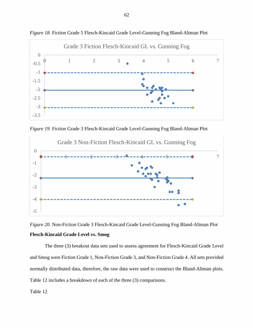
62
Figure 18. Fiction Grade 5 Flesch-Kincaid Grade Level-Gunning Fog Bland-Altman Plot
Figure 19. Fiction Grade 3 Flesch-Kincaid Grade Level-Gunning Fog Bland-Altman Plot
Figure 20. Non-Fiction Grade 3 Flesch-Kincaid Grade Level-Gunning Fog Bland-Altman Plot
Flesch-Kincaid Grade Level vs. Smog
The three (3) breakout data sets used to assess agreement for Flesch-Kincaid Grade Level
and Smog were Fiction Grade 1, Non-Fiction Grade 3, and Non-Fiction Grade 4. All sets provided
normally distributed data, therefore, the raw data were used to construct the Bland-Altman plots.
Table 12 includes a breakdown of each of the three (3) comparisons.
Table 12
-3.5
-3
-2.5
-2
-1.5
-1
-0.5
0
0 1 2 3 4 5 6 7
Grade 3 Fiction Flesch-Kincaid GL vs. Gunning Fog
-5
-4
-3
-2
-1
0
0 1 2 3 4 5 6 7
Grade 3 Non-Fiction Flesch-Kincaid GL vs. Gunning Fog

63
Flesch-Kincaid Grade Level vs. Smog Fiction Grade 1 Non-Fiction Grade 3 Non-Fiction Grade 4
Mean (Bias) -1.72759 -0.65 -0.544828
SD 0.721059 0.888052 0.795337
Upper LOA -0.31431 1.090582 1.014034
Lower LOA -3.14086 -2.390582 -2.103689
Spread LOA 2.826551 3.481164 3.117723
Percentage error n/a* n/a* 0.696
Correlation -0.197 0.265 0.162
*Note: percentage error not appropriate possibly due to extreme outliers
The difference for both Non-Fiction Grade 3 and Non-Fiction Grade 4 were within the a
priori defined 1.5 grade levels suggesting possible agreement. The Fiction Grade 1 set exceeds the
allowed 1.5 grade levels suggesting the two indexes lack agreement. The two Non-Fiction sets
appear to have proportional error based on the Bland-Altman plots. Figures 21-22 include the
Bland-Altman plots for both Non-Fiction sets. In both cases, as the average increases the difference
decreases. Although data points for both plots fall within the limits of agreement, the proportional
error suggests that the two measures do not agree. The Non-Fiction Grades 1-5 Bland-Altman plot
does suggest agreement with an acceptable difference between the two measures and a narrow
limit of agreement. See Appendix B for the Bland-Altman plot.

64
Figure 21. Non-Fiction Grade 3 Flesch-Kincaid Grade Level-Smog Bland-Altman Plot
Figure 22. Non-Fiction Grade 4 Flesch-Kincaid Grade Level-Smog Bland Altman Plot
Fry Graph vs. Dale-Chall
The three (3) breakout data sets used to assess agreement for Fry Graph and Dale-Chall
were Fiction Grade 4, Non-Fiction Grade 3, and Non-Fiction Grade 5. The Fiction Grade 4 and
Non-Fiction Grade 5 sets provided normally distributed data, therefore, the raw data were used to
construct the Bland-Altman plots. The Fiction Grade 3, however, provided non-normal distribution
of data. Ratio transformations were performed on this set of data. The ratio data were used to create
the Bland-Altman plot. Table 13 includes a breakdown of each of the three (3) comparisons.
-3
-2
-1
0
1
2
3
0 1 2 3 4 5 6
Grade 3 Non-Fiction Flesch-Kincaid GL vs. Smog
-2.5
-2
-1.5
-1
-0.5
0
0.5
1
1.5
0 1 2 3 4 5 6 7
Grade 4 Non-Fiction Flesch-Kincaid GL vs. Smog

65
Table 13
Fry Graph vs. Dale-Chall Fiction Grade 4 Non-Fiction Grade 3 (ratio) Non-Fiction Grade 5
Mean (Bias) -0.65556 0.855907 -0.841935
SD 1.380206 0.154879 0.919701
Upper LOA 2.049647 1.159468 0.960678
Lower LOA -3.36076 0.552345 -2.644549
Spread LOA 5.410406 0.607124 3.605227
Percentage error n/a* 0.1263 0.7501
Correlation -0.334 0.155 0.155
*Note: percentage error not appropriate possibly due to extreme outliers
The difference of each set falls within the allowed 1.5 grade levels suggesting possible
agreement. Each Bland-Altman plot however reveals an interesting pattern. As the average
increases in each set, the difference decreases in a linear fashion. The linear sets of data do not
suggest a relationship between differences and averages, as would be expected when two measures
agree. When two measures agree, the scatter of data points falls near the bias line. There appears
to be both fixed and proportional bias between these two measures. A large measure of
proportional error was detected in the Non-Fiction Grade 5 data set. The spread of the LoA also
appears to be wider than desired when evaluating for agreement, especially for Fiction Grade 4
and Non-Fiction Grade 5. While data points for both plots fall within the limits of agreement, the
proportional error suggests that the two measures do not agree. The Bland-Altman plots for Fry
Graph vs. Dale-Chall are in Figures 23-25.

66
Figure 23. Fiction Grade 4 Fry Graph-Dale-Chall Bland-Altman Plot
Figure 24. Non-Fiction Grade 3 Fry Graph-Dale-Chall Bland-Altman Plot
-5
-4
-3
-2
-1
0
1
2
3
0 1 2 3 4 5 6 7 8
Grade 4 Fiction Fry Graph vs. Dale-Chall
0
0.2
0.4
0.6
0.8
1
1.2
1.4
0 1 2 3 4 5 6 7 8
Grade 3 Non-Fiction (Ratio) Fry Graph vs. Dale-Chall

67
Figure 25. Non-Fiction Grade 5 Fry Graph-Dale-Chall Bland-Altman Plot
Fry Graph vs. Spache
The three (3) breakout data sets used to assess agreement for Fry Graph and Spache were
Fiction Grade 1, Non-Fiction Grade 1, and Non-Fiction Grade 2. All sets provided normally
distributed data, therefore, the raw data were used to construct the Bland-Altman plots. Table 14
includes a breakdown of each of the three (3) comparisons.
Table 14
Fry Graph vs. Spache Fiction Grade 1 Non-Fiction Grade 1 Non-Fiction Grade 2
Mean (Bias) -1.24138 -0.7111 -0.27667
SD 0.770676 0.998757 1.032467
Upper LOA 0.269145 1.246453 1.746969
Lower LOA -2.7519 -2.668676 -2.3003
Spread LOA 3.0210 3.915129 4.047271
Percentage error n/a* n/a* n/a*
Correlation 0.20 0.24 -0.08
*Note: percentage error not appropriate possibly due to extreme outliers
-3
-2
-1
0
1
2
0 1 2 3 4 5 6 7 8
Grade 5 Non-Fiction Fry Graph vs. Dale-Chall

68
The difference of each set falls within the allowed 1.5 grade levels suggesting possible
agreement. Each Bland-Altman plot, however, reveals an interesting pattern. As the average
increases in each set, the difference decreases in a linear fashion. The linear sets of data do not
suggest a relationship between differences and averages, as would be expected when two measures
agree. When two measures agree the scatter of data points will fall near the bias line. There appears
to be strong proportional bias between these two measures, as well as fixed bias. The spread of the
LoA also appears to be wider than desired when evaluating for agreement for all data sets. While
the majority of data points for both plots fall within the limits of agreement, the proportional error
suggests that the two measures do not agree.
The Bland-Altman plots for each Fry Graph-Spache data set are in Figures 26-28.
Figure 26. Fiction Grade 1 Fry Graph-Spache Bland-Altman Plot
-3
-2.5
-2
-1.5
-1
-0.5
0
0.5
1
0 0.5 1 1.5 2 2.5 3 3.5 4
Grade 1 Fiction Fry Graph vs. Spache

69
Figure 27. Non-Fiction Grade 1 Fry Graph-Spache Bland-Altman Plot
Figure 28. Non-Fiction Grade 2 Fry Graph-Spache Bland-Altman Plot
Fry Graph vs. Gunning Fog
The three (3) breakout data sets used to assess agreement for Fry Graph and Gunning Fog
were Fiction Grade 5, Non-Fiction Grade 2, and Non-Fiction Grade 3. The Non-Fiction Grade 2
and Non-Fiction Grade 3 sets provided normally distributed data, therefore, the raw data were used
to construct the Bland-Altman plots. The Fiction Grade 5, however, provided non-normal
distribution of data. Ratio transformations were performed on this set of data. The ratio data were
used to create the Bland-Altman plot. Table 15 includes a breakdown of each of the three (3)
-4
-3
-2
-1
0
1
2
0 1 2 3 4 5
Grade 1 Non-Fiction Fry Graph vs. Spache
-3
-2
-1
0
1
2
0 1 2 3 4 5
Grade 2 Non-Fiction Fry Graph vs. Spache

70
comparisons.
The difference of each set falls within the allowed 1.5 grade levels suggesting possible
agreement. Again, each Bland-Altman plot reveals an interesting pattern. As the average increases
in each set, the difference decreases in a linear fashion. This appears to be a pattern when
evaluating data with the Fry Graph readability index. The linear sets of data do not suggest a
relationship between differences and averages, as would be expected when two measures agree.
When two measures agree the scatter of data points will fall near the bias line. The data being
analyzed do not fall consistently near the bias line.
Table 15
Fry Graph vs. Gunning Fog Fiction Grade 5 Non-Fiction Grade 2 Non-Fiction Grade 3
Mean (Bias) 0.887186 -1.41667 -1.02353
SD 0.175769 1.007244 1.192161
Upper LOA 1.231694 0.557531 1.313106
Lower LOA 0.542678 -3.39086 -3.36016
Spread LOA 0.689015 3.948396 4.673271
Percentage error 0.113 n/a* 0.99
Correlation 0.613 0.184 0.174
*Note: percentage error not appropriate possibly due to extreme outliers
There appears to be strong proportional bias between these two measures, as well as fixed
bias. The spread of the LoA also appears to be wider than desired when evaluating for agreement
for all data sets. Although the majority of data points for both plots fall within the limits of
agreement, there appear to be several outliers. The proportional error suggests that the two
measures do not agree. The Bland-Altman plots for each Fry Graph-Gunning Fog data set are in
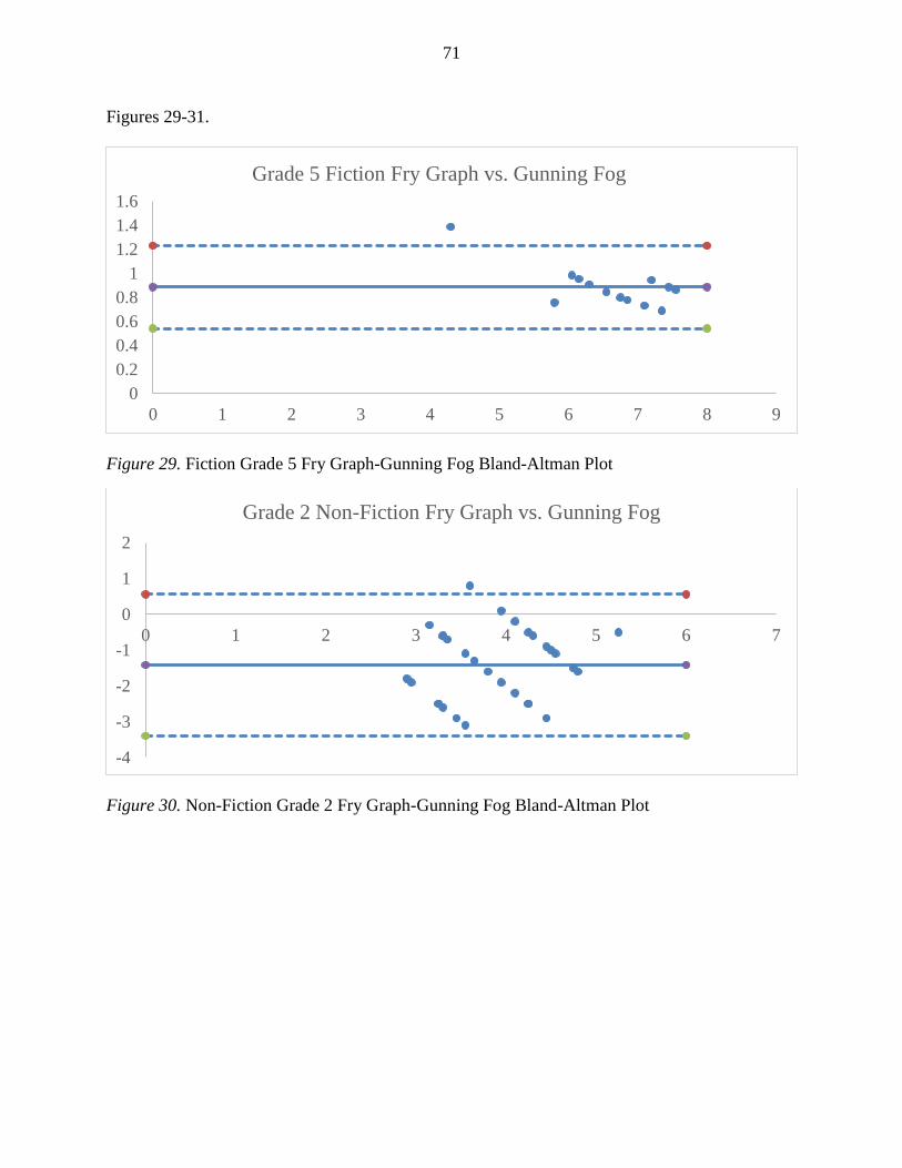
71
Figures 29-31.
Figure 29. Fiction Grade 5 Fry Graph-Gunning Fog Bland-Altman Plot
Figure 30. Non-Fiction Grade 2 Fry Graph-Gunning Fog Bland-Altman Plot
0
0.2
0.4
0.6
0.8
1
1.2
1.4
1.6
0 1 2 3 4 5 6 7 8 9
Grade 5 Fiction Fry Graph vs. Gunning Fog
-4
-3
-2
-1
0
1
2
0 1 2 3 4 5 6 7
Grade 2 Non-Fiction Fry Graph vs. Gunning Fog

72
Figure 31. Non-Fiction Grade 3 Fry Graph-Gunning Fog Bland-Altman Plot
Fry Graph vs. Smog
The three (3) breakout data sets used to assess agreement for Fry Graph and Smog were
Fiction Grade 1, Fiction Grade 5, and Non-Fiction Grade 3. All sets provided normally distributed
data, therefore, the raw data were used to construct the Bland-Altman plots. Table 16 includes a
breakdown of each of the three (3) comparisons.
Table 16
Fry Graph vs. Smog Fiction Grade 1 Fiction Grade 5 Non-Fiction Grade 3
Mean (Bias) -1.39655 0.976923 0.582353
SD 0.902173 0.881432 1.174855
Upper LOA 0.371708 5.092923 2.88507
Lower LOA -3.16481 -3.13908 -1.72036
Spread LOA 3.536518 8.232 4.605433
Percentage error n/a* n/a* 0.979
Correlation 0.007 0.346 0.141
*Note: percentage error not appropriate possibly due to extreme outliers
-5
-4
-3
-2
-1
0
1
2
0 1 2 3 4 5 6 7 8
Grade 3 Non-Fiction Fry Graph vs. Gunning Fog
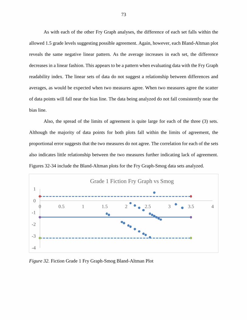
73
As with each of the other Fry Graph analyses, the difference of each set falls within the
allowed 1.5 grade levels suggesting possible agreement. Again, however, each Bland-Altman plot
reveals the same negative linear pattern. As the average increases in each set, the difference
decreases in a linear fashion. This appears to be a pattern when evaluating data with the Fry Graph
readability index. The linear sets of data do not suggest a relationship between differences and
averages, as would be expected when two measures agree. When two measures agree the scatter
of data points will fall near the bias line. The data being analyzed do not fall consistently near the
bias line.
Also, the spread of the limits of agreement is quite large for each of the three (3) sets.
Although the majority of data points for both plots fall within the limits of agreement, the
proportional error suggests that the two measures do not agree. The correlation for each of the sets
also indicates little relationship between the two measures further indicating lack of agreement.
Figures 32-34 include the Bland-Altman plots for the Fry Graph-Smog data sets analyzed.
Figure 32. Fiction Grade 1 Fry Graph-Smog Bland-Altman Plot
-4
-3
-2
-1
0
1
0 0.5 1 1.5 2 2.5 3 3.5 4
Grade 1 Fiction Fry Graph vs Smog

74
Figure 33. Fiction Grade 5 Fry Graph-Smog Bland-Altman Plot
Figure 34. Non-Fiction Grade 3 Fry Graph-Smog Bland-Altman Plot
Dale-Chall vs. Spache
The three (3) breakout data sets used to assess agreement for Dale-Chall and Spache were
Fiction Grade 4, Non-Fiction Grade 1, and Non-Fiction Grade 3. The Fiction Grade 4 set provided
normally distributed data, therefore, the raw data were used to construct the Bland-Altman plot for
this data. The Non-Fiction Grade 1 and the Non-Fiction Grade 3 data sets, however, provided non-
normal distribution of data. A ratio transformation was performed. The ratio data were used to
create the Bland-Altman plots. Table 17 includes a breakdown of each of the three (3)
-4
-2
0
2
4
6
0 1 2 3 4 5 6 7 8 9
Grade 5 Fiction Fry Graph vs. Smog
-2
-1
0
1
2
3
4
0 1 2 3 4 5 6 7 8
Grade 3 Non-Fiction Fry Graph vs. Smog

75
comparisons.
Table 17
Dale-Chall vs. Spache Fiction Grade
4
Non-Fiction Grade 1
(Ratio)
Non-Fiction Grade 3
(ratio)
Mean (Bias) 1.78333 1.30918 1.41584
SD 0.59926 0.66419 0.44768
Upper LOA 2.95789 2.61099 2.2933
Lower LOA 0.60878 0.00074 0.53838
Spread LOA 2.349 2.604 1.755
Percentage
error
0.40 0.618 0.337
Correlation -0.1667 0.67 0.40
The difference for the Fiction Grade 4 data appears to exceed the 1.5 grade levels limit for
agreement. The non-fiction sets were calculated using ratio data, however, the raw data difference
falls within the 1.5 grade levels limit for agreement. The difference for Non-Fiction Grade 1 is
1.111 and the difference for Non-Fiction Grade 3 is 1.489, each suggesting possible agreement
between methods. The spread of the limits of agreement are more narrow than other comparisons,
however, each set does have some degree of proportional error. The Bland-Altman plots for the
two non-fiction sets reveal several outliers that may skew the data making it difficult to assess
agreement between the two methods. Figures 35-36 contain the two data comparisons for the non-
fiction data.

76
Figure 35. Non-Fiction Grade 1 Dale-Chall-Spache Bland-Altman Plot
Figure 36. Non-Fiction Grade 3 Dale-Chall-Spache Bland-Altman Plot
In comparison, the Fiction Grade 4 Bland-Altman plot (see Figure 37) has a narrow spread of
limits of agreement, however, the difference exceeds the 1.5 grade levels and a percentage error
of 0.40 indicating proportional error exists within this data set.
0
0.5
1
1.5
2
2.5
3
0 1 2 3 4 5 6 7
Grade 1 Non-Fiction (Ratio) Dale-Chall vs. Spache
0
0.5
1
1.5
2
2.5
0 1 2 3 4 5 6 7 8
Grade 3 Non-Fiction (Ratio) Dale-Chall vs. Spache

77
Figure 37. Fiction Grade 4 Dale-Chall-Spache Bland-Altman plot
Dale-Chall vs. Gunning Fog
The three (3) breakout data sets used to assess agreement for Dale-Chall and Gunning Fog
were Fiction Grade 2, Non-Fiction Grade 2, and Non-Fiction Grade 4. All three (3) sets of data
provided non-normal distribution of data. A ratio transformation was performed. The ratio data
were used to create the Bland-Altman plots. Table 18 includes a breakdown of each of the three
(3) comparisons.
Table 18
Dale-Chall vs. Gunning Fog Fiction Grade 2
(Ratio)
Non-Fiction Grade 2
(ratio)
Non-Fiction Grade 4
(ratio)
Mean (Bias) 1.445176 1.091492 0.858602
SD 0.415778 0.43523 0.227992
Upper LOA 2.260102 1.944543 1.305467
Lower LOA 0.63025 0.238442 0.411737
Spread LOA 1.629851 1.706101 0.89373
0
0.5
1
1.5
2
2.5
3
3.5
0 1 2 3 4 5 6 7
Grade 4 Fiction Dale-Chall vs. Spache

78
Percentage
error
0.275 0.352 0.16
Correlation -0.218 -0.0997 -0.161
The difference for the Fiction Grade 2 data appears to exceed the 1.5 grade levels limit for
agreement based on the actual difference calculated for the raw data. The difference for this set
was 1.6333. The non-fiction sets were also calculated using ratio data, however, the raw data
difference falls within the 1.5 grade levels limit for agreement. The difference for Non-Fiction
Grade 2 is 0.267 and the difference for Non-Fiction Grade 4 is -1.11, each suggesting possible
agreement between methods. The spread of the limits of agreement are more narrow than other
comparisons, also supporting possible agreement between the two methods. Proportional error
remains low and may exist due to several outliers within the data sets. These outliers are apparent
in the Bland-Altman plots in Figures 38-40. There appears to be agreement between the two
measures when looking at the non-fiction data for each of the grade levels analyzed.
Figure 38. Fiction Grade 2 Dale-Chall-Gunning Fog Bland-Altman Plot
0
0.5
1
1.5
2
2.5
3
3.5
0 1 2 3 4 5 6 7 8
Grade 2 Fiction (Ratio) Dale-Chall vs. Gunning Fog

79
Figure 39. Non-Fiction Grade 2 Dale-Chall-Gunning Fog Bland-Altman Plot
Figure 40. Non-Fiction Grade 4 Dale-Chall-Gunning Fog Bland-Altman Plot
Dale-Chall vs. Smog
The three (3) breakout data sets used to assess agreement for Dale-Chall and Smog were
Fiction Grade 1, Non-Fiction Grade 1, and Non-Fiction Grade 4. All three (3) sets of data provided
non-normal distribution of data. A ratio transformation was performed. The ratio data were used
to create the Bland-Altman plots. Table 19 includes a breakdown of each of the three (3)
comparisons.
Table 19
0
0.5
1
1.5
2
2.5
0 1 2 3 4 5 6 7 8
Grade 2 Non-Fiction (Ratio) Dale-Chall vs. Gunning Fog
0
0.2
0.4
0.6
0.8
1
1.2
1.4
1.6
0 1 2 3 4 5 6 7 8 9
Grade 4 Non-Fiction (Ratio) Dale-Chall vs. Gunning Fog
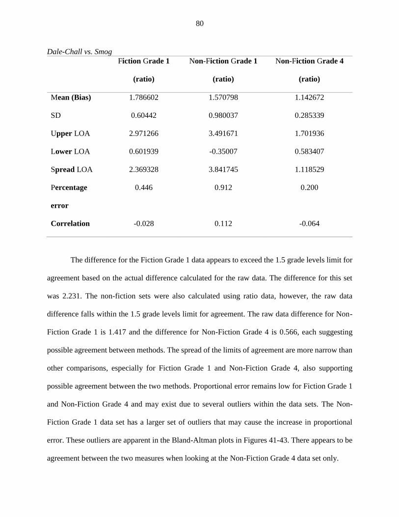
80
Dale-Chall vs. Smog Fiction Grade 1
(ratio)
Non-Fiction Grade 1
(ratio)
Non-Fiction Grade 4
(ratio)
Mean (Bias) 1.786602 1.570798 1.142672
SD 0.60442 0.980037 0.285339
Upper LOA 2.971266 3.491671 1.701936
Lower LOA 0.601939 -0.35007 0.583407
Spread LOA 2.369328 3.841745 1.118529
Percentage
error
0.446 0.912 0.200
Correlation -0.028 0.112 -0.064
The difference for the Fiction Grade 1 data appears to exceed the 1.5 grade levels limit for
agreement based on the actual difference calculated for the raw data. The difference for this set
was 2.231. The non-fiction sets were also calculated using ratio data, however, the raw data
difference falls within the 1.5 grade levels limit for agreement. The raw data difference for Non-
Fiction Grade 1 is 1.417 and the difference for Non-Fiction Grade 4 is 0.566, each suggesting
possible agreement between methods. The spread of the limits of agreement are more narrow than
other comparisons, especially for Fiction Grade 1 and Non-Fiction Grade 4, also supporting
possible agreement between the two methods. Proportional error remains low for Fiction Grade 1
and Non-Fiction Grade 4 and may exist due to several outliers within the data sets. The Non-
Fiction Grade 1 data set has a larger set of outliers that may cause the increase in proportional
error. These outliers are apparent in the Bland-Altman plots in Figures 41-43. There appears to be
agreement between the two measures when looking at the Non-Fiction Grade 4 data set only.

81
Both the Fiction Grades 1-5 and Non-Fiction Grades 1-5 produce Bland-Altman plots that
suggest agreement between the two measures. The difference of each is within the 1.5 grade levels
and both have a narrow limit of agreement. See Appendix B for the Bland-Altman plots.
Figure 41. Fiction Grade 1 Dale-Chall-Smog Bland-Altman Plot
Figure 42. Non-Fiction Grade 1 Dale-Chall-Smog Bland-Altman Plot
0
0.5
1
1.5
2
2.5
3
3.5
0 1 2 3 4 5 6 7
Grade 1 Fiction (Ratio) Dale-Chall vs. Smog
-1
0
1
2
3
4
0 1 2 3 4 5 6 7
Grade 1 Non-Fiction (Ratio) Dale-Chall vs. Smog

82
Figure 43. Non-Fiction Grade 4 Dale-Chall-Smog Bland-Altman Plot
Spache vs. Smog
The three (3) breakout data sets used to assess agreement for Spache and Smog were
Fiction Grade 4, Non-Fiction Grade 2, and Non-Fiction Grade 3. All sets provided normally
distributed data, therefore, the raw data were used to construct the Bland-Altman plots. Table 20
includes a breakdown of each of the three (3) comparisons.
Table 20
Spache vs. Smog Fiction Grade 1 Non-Fiction Grade 2 Non-Fiction Grade 3
Mean (Bias) -0.344444 -0.06 -0.40294
SD 0.766368 0.861674 1.268615
Upper LOA 1.157637 1.628882 2.083545
Lower LOS -1.846526 -1.74888 -2.88943
Spread LOA 3.004163 3.377764 4.972972
Percentage error 0.734 0.981 n/a*
Correlation 0.126 0.088 -0.139
*Note: percentage error not appropriate possibly due to extreme outliers
0
0.5
1
1.5
2
0 1 2 3 4 5 6 7 8
Grade 4 Non-Fiction (Ratio) Dale-Chall vs. Smog

83
The difference for each of the data sets falls within the a priori set 1.5 grade levels
suggesting possible agreement. The spread of the limits of agreement for each set is wide and the
percentage error for all sets is high, therefore, proportional error exists within all data sets analyzed.
Based on the Bland-Altman plots in Figures 44-46, several outliers exist within each data set and
the scatter of data points is less condensed around the bias line than desirable. The data do not
support agreement between the two measures.
Figure 44. Fiction Grade 4 Spache-Smog Bland-Altman Plot
Figure 45. Non-Fiction Grade 2 Spache-Smog Bland-Altman Plot
-2.5
-2
-1.5
-1
-0.5
0
0.5
1
1.5
0 1 2 3 4 5 6 7
Grade 4 Fiction Spache vs. Smog
-2
-1.5
-1
-0.5
0
0.5
1
1.5
2
0 1 2 3 4 5 6
Grade 2 Non-Fiction Spache vs. Smog

84
Figure 46. Non-Fiction Grade 3 Spache-Smog Bland-Altman Plot
Gunning Fog vs. Smog
The three (3) breakout data sets used to assess agreement for Gunning Fog and Smog were
Fiction Grade 2, Fiction Grade 5, and Non-Fiction Grade 3. The Fiction Grade 2 and Fiction Grade
5 data sets provided normally distributed data, therefore, the raw data were used to construct the
Bland-Altman plots for these data sets. The Non-Fiction Grade 3 data set, however, provided non-
normal distribution of data. A ratio transformation was performed. The ratio data were used to
create the Bland-Altman plot. Table 21 includes a breakdown of each of the three (3) comparisons.
Table 21
Gunning Fog vs. Smog Fiction Grade 2 Fiction Grade 5 Non-Fiction Grade 3 (ratio)
Mean (Bias) 0.61 1.961538 1.426775
SD 0.554822 1.726528 0.284959
Upper LOA 1.697451 5.345532 1.985295
Lower LOA -0.47745 -1.422456 0.868254
Spread LOA 2.174903 6.767988 1.117041
-4
-3
-2
-1
0
1
2
3
0 1 2 3 4 5 6 7
Grade 3 Non-Fiction Spache vs. Smog

85
Percentage error 0.507 0.958 0.195
Correlation 0.726 -0.235 0.85
The difference for the Fiction Grade 2 set meets the 1.5 grade levels and has an acceptable
spread for limits of agreement. The percentage error at 0.507, however, suggests proportional error
within the data set. Therefore, the two measures do not appear to agree for Fiction Grade 2.
The difference for Fiction Grade 5 and Non-Fiction Grade 3 exceeds the 1.5 grade levels
set for agreement. The Non-Fiction Grade 3 data were calculated using ratio transformations
therefore it is necessary to look at the raw data difference which was 1.605882. Based on the
Bland-Altman plot for Non-Fiction Grade 3 in Figure 47, the data are scattered in a condensed
manner around the bias line with the exception of one outlier. This may contribute to the slightly
raised difference. The spread of the limits of agreement is narrow and the proportional error is low.
However, removing the outlier from the data set does not lower the difference enough to fall within
the a priori set limits of 1.5 grade levels for agreement. Therefore, the data analyzed do not suggest
agreement between the two measures. The Bland-Altman plots for Fiction Grade 2 and Fiction
Grade 5 are in Figures 48-49.
0
0.5
1
1.5
2
2.5
3
0 1 2 3 4 5 6 7 8 9
Grade 3 Non-Fiction (Ratio) Gunning Fog vs. Smog
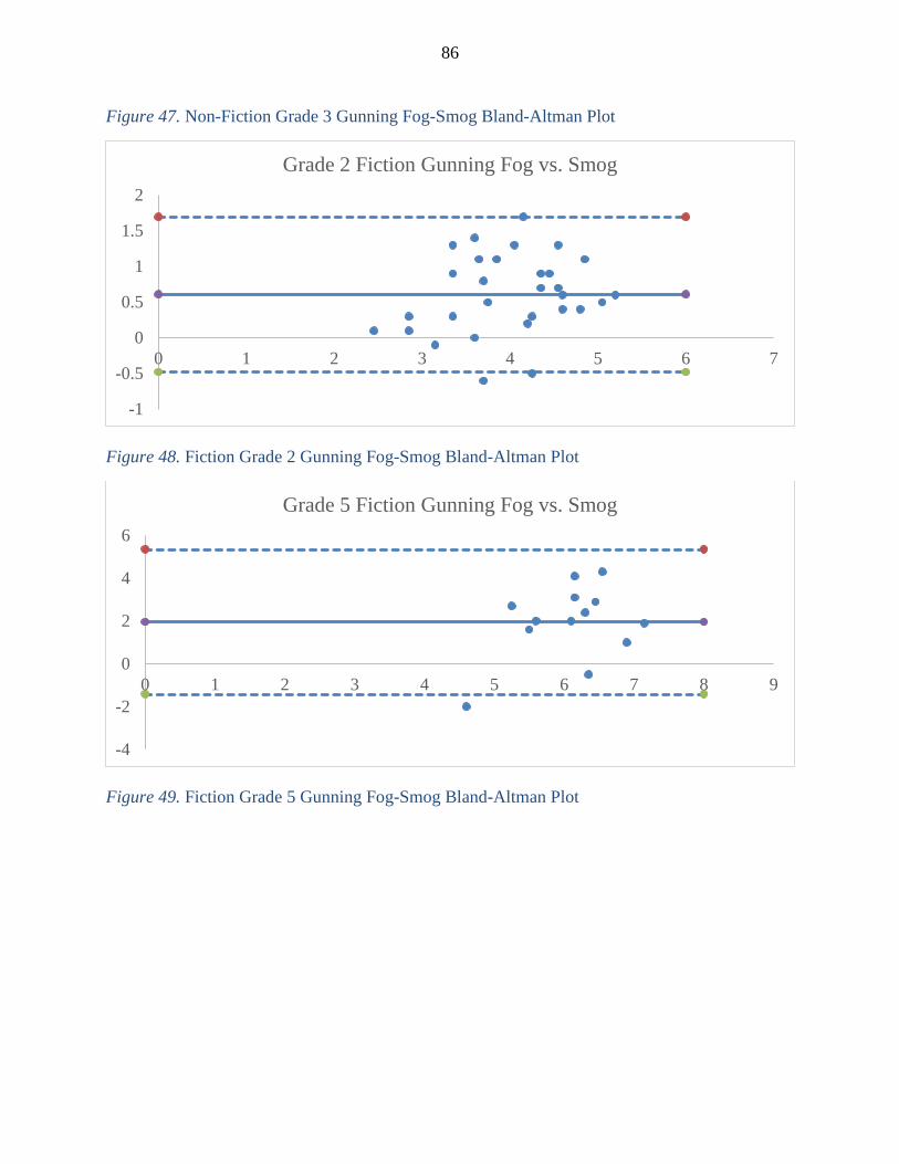
86
Figure 47. Non-Fiction Grade 3 Gunning Fog-Smog Bland-Altman Plot
Figure 48. Fiction Grade 2 Gunning Fog-Smog Bland-Altman Plot
Figure 49. Fiction Grade 5 Gunning Fog-Smog Bland-Altman Plot
-1
-0.5
0
0.5
1
1.5
2
0 1 2 3 4 5 6 7
Grade 2 Fiction Gunning Fog vs. Smog
-4
-2
0
2
4
6
0 1 2 3 4 5 6 7 8 9
Grade 5 Fiction Gunning Fog vs. Smog

87
CHAPTER 5 Conclusions and Recommendations
The Bland-Altman plot was used to assess agreement between six (6) reading indices. The
resulting fifteen (15) analyses resulted in agreement, or near agreement, among nine (9)
comparisons. Near agreement was determined when the difference between the two instruments
was just slightly over the 1.5 grade level set a priori but still resulted in narrow limits of agreement,
low proportional error, and produced a Bland-Altman plot where data points clustered around the
bias line. The spread of the limits of agreement is narrow when instruments suggest agreement
(Myles & Cui, 2007; Moen, 2016). Stevens et al. (2015) pointed out that with this method of
agreement, the probability deemed to suggest agreement and therefore interchangeability is
context-specific and is not a statistical decision. This decision is subjective and is determined based
on subject-matter expertise. The set standard can be less conservative in a practical, education
setting as opposed to a clinical setting where the consequences of the results could cause physical
harm.
The Bland-Altman plot is inappropriate if there is any variability between measures. This
discrepancy was found when attempting to compare Flesch Reading Ease and Coh-Metrix L2 with
any of the other six (6) indexes. Flesch-Kincaid Grade Level, Fry Graph, Spache, Gunning Fog,
Dale-Chall and Smog all provide a construct equivalent to a grade level. Flesch Reading Ease
provides a numerical value 0-100, not a grade level equivalent. Flesch-Kincaid Grade Level
converts the Flesch Reading Ease score into a grade-level equivalency based on the American
grade-level system (Burke, 2010). Coh-Metrix L2 provides a numerical value rooted in text-based
processes and cohesion features (Crossley, Greenfield, & McNamara, 2008; Graesser, McNamara,
Louwerse, & Zhiquiang, 2004; Gallagher, Fazio, & Gunning, 2012). It was deemed necessary to
remove the two (2) indexes from the study due to the discrepant measures.

88
Several of the comparisons rendered non-normal, or heteroscedastic, data sets requiring
ratio transformation. According to Chhapola, Kanwal, and Brar (2015), “transformation of data
usually renders the scatter of differences as homoscedastic” (p. 385). The ratio transformation of
data is one method of addressing non-normality. The ratios of two measures can be plotted against
the average of the two measures (Bland & Altman, 1999; Chhapola, Kanwal, & Brar, 2015). The
transformation of data allows Bland-Altman plots to be reasonably robust when encountering non-
normal data. The data are more compressed with less proportional error evident and less influenced
by outliers when using transformed data. This allows for easier interpretation of the data in most
cases.
The Flesch-Kincaid Grade Level index suggested agreement with Dale-Chall and Spache;
and near agreement with Gunning Fog and Smog. The Dale-Chall index suggested agreement with
Gunning Fog and Smog when the genre evaluated was non-fiction; and suggested near agreement
with Spache, when the genre evaluated was non-fiction. The comparison of Dale-Chall and
Gunning Fog when the genre was fiction suggested near agreement with a difference only slightly
higher than the set standard of 1.5 grade levels. The Dale-Chall index proves to be a strong index
to use with non-fiction genre, especially when sample sizes are large. Set comparisons that did not
illustrate agreement have apparent outliers that may affect the outcome of agreement. The Spache
reading index and Gunning Fog appear to agree particularly with large sample sizes. The non-
fiction plot of all grade levels had narrow limits of agreement and a Bland-Altman plot with data
points clustered near the bias line. The fiction plot was similar to the non-fiction plot, however,
the spread of the limits of agreement was slightly wider. These results suggest that Flesch-Kincaid
Grade Level and Dale-Chall can be used interchangeably with each other and with the Spache
index, the Gunning Fog index and the Smog index.

89
The Fry Graph posed several problems when compared to the other reading indexes. Each
of the Bland-Altman plots comparing Fry Graph with another reading index produced a plot
containing linear sets of data points. Figure 50 is an example of a plot outcome using Fry Graph
as the comparison.
Figure 50. Fry Graph Plot Example.
For each comparison, the proportional error is evident, as well as fixed bias. As the average
increases within the data set, the difference decreases. This is consistent among all comparisons
using Fry Graph. While Fry Graph provides a grade level equivalent like each of the other indexes
analyzed, it gives a discreet grade-level value unlike the other five (5) indexes, which provide a
continuous grade-level value. This difference most likely results in the proportional error evident
in all Fry Graph comparisons. Therefore, Bland-Altman may not be an appropriate method of
comparison using Fry Graph.
Practical implications emerged in addition to the evidence of agreement between certain
readability indexes. Bland-Altman plots are quantitative in nature because of the mathematical
manipulation of the data, however, subject-matter expertise is required to determine an appropriate
judgment regarding agreement (Ludbrook, 2010). This gives the practitioner an opportunity to
-3
-2.5
-2
-1.5
-1
-0.5
0
0.5
1
1.5
0 1 2 3 4 5 6 7 8
Grade 5 Non-Fiction Fry Graph vs. Dale-Chall

90
determine which measures more closely relate to one another and provide similar outcomes.
Flesch-Kincaid Grade Level index and Dale-Chall index both suggested agreement or near
agreement with the other indices, with the exception of the Fry Graph. Although the variances
among readability formulas suggest imperfection, they offer probability statements and estimate
text difficulty, making each index appropriate to use alone or interchangeably when determining
text grade-level (Gallagher, Fazio, & Gunning, 2012). Ultimately, the safest and most predictable
means of selecting a readability index for text evaluation would be to choose one instrument and
use it exclusively. This will ensure consistency and provide similar outcomes. It is important to
note, the Dale-Chall formula and the Smog index are recommended for use with texts at Grade 4
level or above (Begeny & Greene, 2014; Gallagher, Fazio, & Gunning, 2012).
Because of the differences among readability formulas, caution must be used when
employing the indices to identify texts for instructional or intervention purposes (Begeny &
Greene, 2014). This study identifies possible agreement, or interchangeability, between reading
indexes. No suggestion regarding the use of a particular index for text identification is endorsed.
There is little evidence that readability indexes are valid measures of text difficulty when compared
to reading performance and must be considered as only one metric for understanding text difficulty
(Begeny & Greene, 2014). Practitioners should utilize readability indexes as one method of
assessing text readability. According to Goldman & Lee (2014) “text selection must also take into
account the match or mismatch between what students bring to particular texts and what
comprehension of those texts requires in the way of knowledge of the conventions of text structure,
disciplinary content, and disciplinary-inquiry practices” (p. 298). Measuring text readability
requires assessing both quantitative and qualitative factors that contribute to text complexity, as
well as task considerations (Gallagher, Fazio, & Gunning, 2012).
91
Limitations of the Study
One limitation of the study is sample sizes. Grade-level sets, as well as genre sets for each
comparison are not equally represented, limiting the extent of the data analyses. Sample sizes
began equal across all grade levels and genres. Due to the discrepancies identified between
publisher leveling and readability index leveling, some samples required removal. This limitation
has also been noted in previous research findings. Other researchers have found that particular
passages are often classified by grade level very differently across varying readability formulas
(Begeny & Greene, 2014; Ardoin, Suldo, Witt, Aldrich, & McDonald, 2005; Ardoin, Williams,
Christ, Klubnik, & Wellborn, 2010; Compton, Appleton, & Hosp, 2004). It also illustrates the
subjectivity of text leveling. Small samples sizes may weaken the findings of the study. Chhapola
et al. (2015) reported when sample size (n) increased, standard error (SE) decreased and the
confidence interval (CI) of limits of agreement were narrower; when n is insufficient, then CI of
limits of agreement are wider.
Time and resources also limited the size of each reading passage. Each passage was
approximately 100-200 words in length. Often a few multisyllabic words can increase the
readability score of a text especially when shorter passages are utilized (Burke, 2010). When
choosing 100 words from a text of 150 pages the chances of the passage representing the
publisher’s stated grade level are greatly reduced. Longer passages would provide more accurate
grade leveling which could impact study outcomes.
Another limitation of the study is failure to consider qualitative features that impact
comprehension and readability. Readability indices provide only one (1) measure to assist
practitioners in text selection whether for instructional or assessment purposes. Many factors need
to be considered when selecting a text: format, reader schema, illustrations, curriculum, book
92
length, and overall text complexity. All these need to be weighed in relation to the reader’s ability.
Finally, the formulae of readability indexes are unique and complex. Some readability
indexes are constructed using specific high frequency words that affect scoring of non-fiction texts.
Non-Fiction texts contain technical, and often scientific, vocabulary that would not appear on high
frequency word lists. They also contain charts, tables, graphs and other diagrams that are not part
of readability calculations. Readability levels are often underestimated in non-fiction text
(Gallagher, Fazio, & Gunning, 2012). Other readability indexes are recommended for specific
grade levels. Calculations in the present study were made using all readability indexes with all
grade level data.
Further Research
Future research could include replicating the current study with larger sample sizes, longer
passages, and including other readability indexes that measure the same construct, grade-level
equivalency, to support or refute the findings of interchangeability within this study. The use of
readability indexes appropriate for specific grade levels should be controlled for within the study.
This would add to the findings and provide significant value to practitioners.
The ambiguous nature of Fry Graph and its lack of compatibility with other readability
indexes represents another outcome from the present study that would warrant further research.
Fry Graph is a well-established measure, however, the presentation of data with discreet values
versus continuous values is problematic. Ludbrook (2010) recommended the use of regression
analysis when calibrating one method against another or to detect bias (fixed or proportional)
between two methods of measurement when the measurements are on an interval scale. Further
research might include identifying a method or instrument, including other means of data
transformation, to compare Fry Graph to other measures that would result in more meaningful

93
data.
Another research consideration is to investigate why two (2) measures, or readability
indexes, that purport to measure grade-level equivalency do not correlate. Bland and Altman
(1983) stated one purpose of the difference plot is to detect a relationship between the differences
and averages. In the absence of an actual relationship, the B-A plot can suggest a significant
relationship exists (Stevens, Steiner, & MacKay, 2015). The reverse can also be true as evident
with Fry Graph. The correlation of Fry Graph with Flesch-Kincaid Grade Level, Gunning Fog and
Smog all indicate a significant relationship between measures but lack agreement.

94
APPENDIX
APPENDIX A: BLAND-ALTMAN PLOTS FOR INDIVIDUAL GRADE LEVELS AND
GENRES
1. Flesch-Kincaid Grade Level vs. Fry Graph
0
0.5
1
1.5
2
0 0.5 1 1.5 2 2.5 3 3.5
Grade 1 Fiction (Ratio) Flesch Kincaid GL vs. Fry Graph
-2
-1.5
-1
-0.5
0
0.5
1
1.5
2
0 0.5 1 1.5 2 2.5 3 3.5 4
Grade 2 Fiction Flesch-Kincaid GL vs. Fry Graph

95
2. Flesch-Kincaid Grade Level vs. Dale-Chall
-3.5
-3
-2.5
-2
-1.5
-1
-0.5
0
0.5
0 1 2 3 4 5 6 7
Grade 3 Non-Fiction Flesch-Kincaid GL vs. Fry Graph
-1
0
1
2
3
4
0 1 2 3 4 5 6 7
Grade 3 Fiction Flesch-Kincaid GL (Ratio) vs. Dale-Chall

96
3. Flesch-Kincaid Grade Level vs. Spache
-3.5
-3
-2.5
-2
-1.5
-1
-0.5
0
0.5
0 1 2 3 4 5 6 7
Grade 4 Non-Fiction Flesch-Kincaid GL vs. Dale-Chall
-3
-2.5
-2
-1.5
-1
-0.5
0
0.5
0 1 2 3 4 5 6 7 8 9
Grade 5 Non-Fiction Flesch-Kincaid GL vs. Dale-Chall

97
0
0.1
0.2
0.3
0.4
0.5
0.6
0.7
0.8
0 0.5 1 1.5 2 2.5 3 3.5 4
Grade 1 Fiction (Ratio) Flesch-Kincaid GL vs. Spache
0
0.2
0.4
0.6
0.8
1
1.2
1.4
1.6
0 1 2 3 4 5 6 7
Grade 5 Fiction (Ratio) Flesch-Kincaid GL vs. Spache
-1.5
-1
-0.5
0
0.5
1
1.5
2
0 1 2 3 4 5 6 7
Grade 4 Non-Fiction Flesch-Kincaid GL vs. Spache

98
4. Flesch-Kincaid Grade Level vs. Gunning Fog
-3.5
-3
-2.5
-2
-1.5
-1
-0.5
0
0 1 2 3 4 5 6 7
Grade 3 Fiction Flesch-Kincaid GL vs. Gunning Fog
0
0.5
1
1.5
2
0 1 2 3 4 5 6 7 8 9
Grade 5 Fiction (Ratio) Flesch-Kincaid GL vs. Gunning Fog
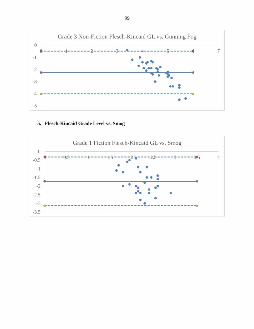
99
5. Flesch-Kincaid Grade Level vs. Smog
-5
-4
-3
-2
-1
0
0 1 2 3 4 5 6 7
Grade 3 Non-Fiction Flesch-Kincaid GL vs. Gunning Fog
-3.5
-3
-2.5
-2
-1.5
-1
-0.5
0
0 0.5 1 1.5 2 2.5 3 3.5 4
Grade 1 Fiction Flesch-Kincaid GL vs. Smog

100
6. Fry Graph vs. Dale-Chall
-3
-2
-1
0
1
2
3
0 1 2 3 4 5 6
Grade 3 Non-Fiction Flesch-Kincaid GL vs. Smog
-2.5
-2
-1.5
-1
-0.5
0
0.5
1
1.5
0 1 2 3 4 5 6 7
Grade 4 Non-Fiction Flesch-Kincaid GL vs. Smog

101
-5
-4
-3
-2
-1
0
1
2
3
0 1 2 3 4 5 6 7 8
Grade 4 Fiction Fry Graph vs. Dale-Chall
0
0.2
0.4
0.6
0.8
1
1.2
1.4
0 1 2 3 4 5 6 7 8
Grade 3 Non-Fiction (Ratio) Fry Graph vs. Dale-Chall
-3
-2
-1
0
1
2
0 1 2 3 4 5 6 7 8
Grade 5 Non-Fiction Fry Graph vs. Dale-Chall

102
7. Fry Graph vs. Spache
-3
-2.5
-2
-1.5
-1
-0.5
0
0.5
1
0 0.5 1 1.5 2 2.5 3 3.5 4
Grade 1 Fiction Fry Graph vs. Spache
-4
-3
-2
-1
0
1
2
0 1 2 3 4 5
Grade 1 Non-Fiction Fry Graph vs. Spache

103
8. Fry Graph vs. Gunning Fog
-3
-2
-1
0
1
2
0 1 2 3 4 5
Grade 2 Non-Fiction Fry Graph vs. Spache
0
0.2
0.4
0.6
0.8
1
1.2
1.4
1.6
0 1 2 3 4 5 6 7 8 9
Grade 5 Fiction Fry Graph vs. Gunning Fog

104
9. Fry Graph vs. Smog
-4
-3
-2
-1
0
1
2
0 1 2 3 4 5 6 7
Grade 2 Non-Fiction Fry Graph vs. Gunning Fog
-5
-4
-3
-2
-1
0
1
2
0 1 2 3 4 5 6 7 8
Grade 3 Non-Fiction Fry Graph vs. Gunning Fog

105
-4
-3
-2
-1
0
1
0 0.5 1 1.5 2 2.5 3 3.5 4
Grade 1 Fiction Fry Graph vs Smog
-4
-2
0
2
4
6
0 1 2 3 4 5 6 7 8 9
Grade 5 Fiction Fry Graph vs. Smog
-2
-1
0
1
2
3
4
0 1 2 3 4 5 6 7 8
Grade 3 Non-Fiction Fry Graph vs. Smog

106
10. Dale-Chall vs. Spache
0
0.5
1
1.5
2
2.5
3
3.5
0 1 2 3 4 5 6 7
Grade 4 Fiction Dale-Chall vs. Spache
0
0.5
1
1.5
2
2.5
3
0 1 2 3 4 5 6 7
Grade 1 Non-Fiction (Ratio) Dale-Chall vs. Spache

107
11. Dale-Chall vs. Gunning Fog
0
0.5
1
1.5
2
2.5
0 1 2 3 4 5 6 7 8
Grade 3 Non-Fiction (Ratio) Dale-Chall vs. Spache
0
0.5
1
1.5
2
2.5
3
3.5
0 1 2 3 4 5 6 7 8
Grade 2 Fiction (Ratio) Dale-Chall vs. Gunning Fog
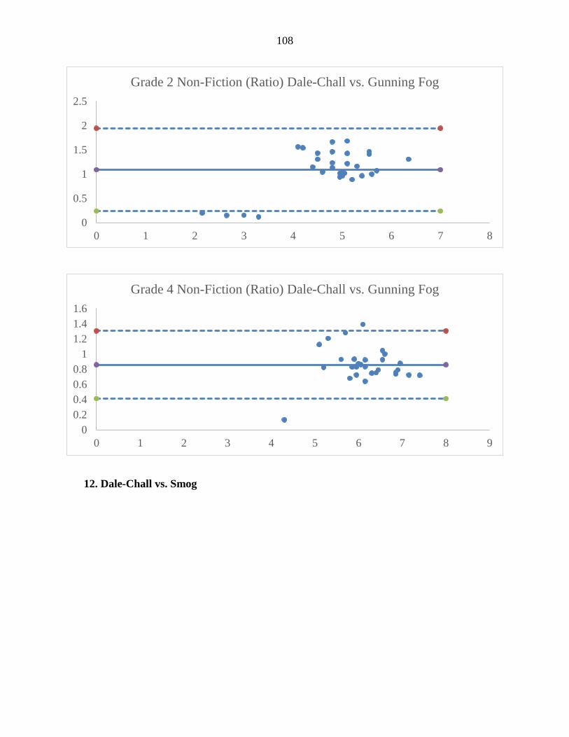
108
12. Dale-Chall vs. Smog
0
0.5
1
1.5
2
2.5
0 1 2 3 4 5 6 7 8
Grade 2 Non-Fiction (Ratio) Dale-Chall vs. Gunning Fog
0
0.2
0.4
0.6
0.8
1
1.2
1.4
1.6
0 1 2 3 4 5 6 7 8 9
Grade 4 Non-Fiction (Ratio) Dale-Chall vs. Gunning Fog

109
0
0.5
1
1.5
2
2.5
3
3.5
0 1 2 3 4 5 6 7
Grade 1 Fiction (Ratio) Dale-Chall vs. Smog
-1
0
1
2
3
4
0 1 2 3 4 5 6 7
Grade 1 Non-Fiction (Ratio) Dale-Chall vs. Smog
0
0.5
1
1.5
2
0 1 2 3 4 5 6 7 8
Grade 4 Non-Fiction (Ratio) Dale-Chall vs. Smog

110
13. Spache vs. Gunning Fog
-4
-3
-2
-1
0
1
0 1 2 3 4 5 6 7
Grade 3 Fiction Spache vs. Gunning Fog
-3.5
-3
-2.5
-2
-1.5
-1
-0.5
0
0.5
1
0 1 2 3 4 5 6 7
Grade 2 Non-Fiction Spache vs. Gunning Fog
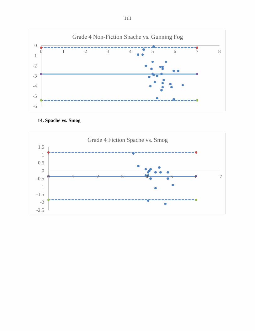
111
14. Spache vs. Smog
-6
-5
-4
-3
-2
-1
0
0 1 2 3 4 5 6 7 8
Grade 4 Non-Fiction Spache vs. Gunning Fog
-2.5
-2
-1.5
-1
-0.5
0
0.5
1
1.5
0 1 2 3 4 5 6 7
Grade 4 Fiction Spache vs. Smog

112
15. Gunning Fog vs. Smog
-2
-1.5
-1
-0.5
0
0.5
1
1.5
2
0 1 2 3 4 5 6
Grade 2 Non-Fiction Spache vs. Smog
-4
-3
-2
-1
0
1
2
3
0 1 2 3 4 5 6 7
Grade 3 Non-Fiction Spache vs. Smog

113
-1
-0.5
0
0.5
1
1.5
2
0 1 2 3 4 5 6 7
Grade 2 Fiction Gunning Fog vs. Smog
-4
-2
0
2
4
6
0 1 2 3 4 5 6 7 8 9
Grade 5 Fiction Gunning Fog vs. Smog
0
0.5
1
1.5
2
2.5
3
0 1 2 3 4 5 6 7 8 9
Grade 3 Non-Fiction (Ratio) Gunning Fog vs. Smog

114
APPENDIX B: BLAND-ALTMAN PLOTS BY GENRE, ALL GRADE LEVELS
-3
-2
-1
0
1
2
3
0 1 2 3 4 5 6 7 8
Fiction Flesch-Kincaid GL vs. Fry Graph
0
0.2
0.4
0.6
0.8
1
1.2
1.4
0 1 2 3 4 5 6 7 8 9
Non-Fiction Flesch-Kincaid GL vs. Fry Graph

115
-8
-6
-4
-2
0
2
4
0 1 2 3 4 5 6 7 8
Fiction Flesch-Kincaid GL vs. Dale-Chall
-2
0
2
4
6
8
10
12
0 1 2 3 4 5 6 7 8 9
Non-Fiction Flesch-Kincaid GL vs. Dale-Chall
0
0.2
0.4
0.6
0.8
1
1.2
1.4
1.6
0 1 2 3 4 5 6 7
Fiction Flesch-Kincaid GL vs. Spache

116
-4
-3
-2
-1
0
1
2
3
0 1 2 3 4 5 6 7 8
Non-Fiction Flesch-Kincaid GL vs. Spache
0
0.5
1
1.5
2
0 1 2 3 4 5 6 7 8 9
Fiction Flesch-Kincaid GL vs. Gunning Fog
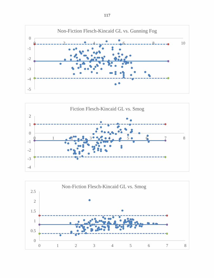
117
-5
-4
-3
-2
-1
0
0 2 4 6 8 10
Non-Fiction Flesch-Kincaid GL vs. Gunning Fog
-4
-3
-2
-1
0
1
2
0 1 2 3 4 5 6 7 8
Fiction Flesch-Kincaid GL vs. Smog
0
0.5
1
1.5
2
2.5
0 1 2 3 4 5 6 7 8
Non-Fiction Flesch-Kincaid GL vs. Smog

118
-1
0
1
2
3
4
0 1 2 3 4 5 6 7 8 9
Fiction Fry Graph vs. Dale-Chall
-6
-4
-2
0
2
4
6
0 2 4 6 8 10
Non-Fiction Fry Graph vs. Dale-Chall
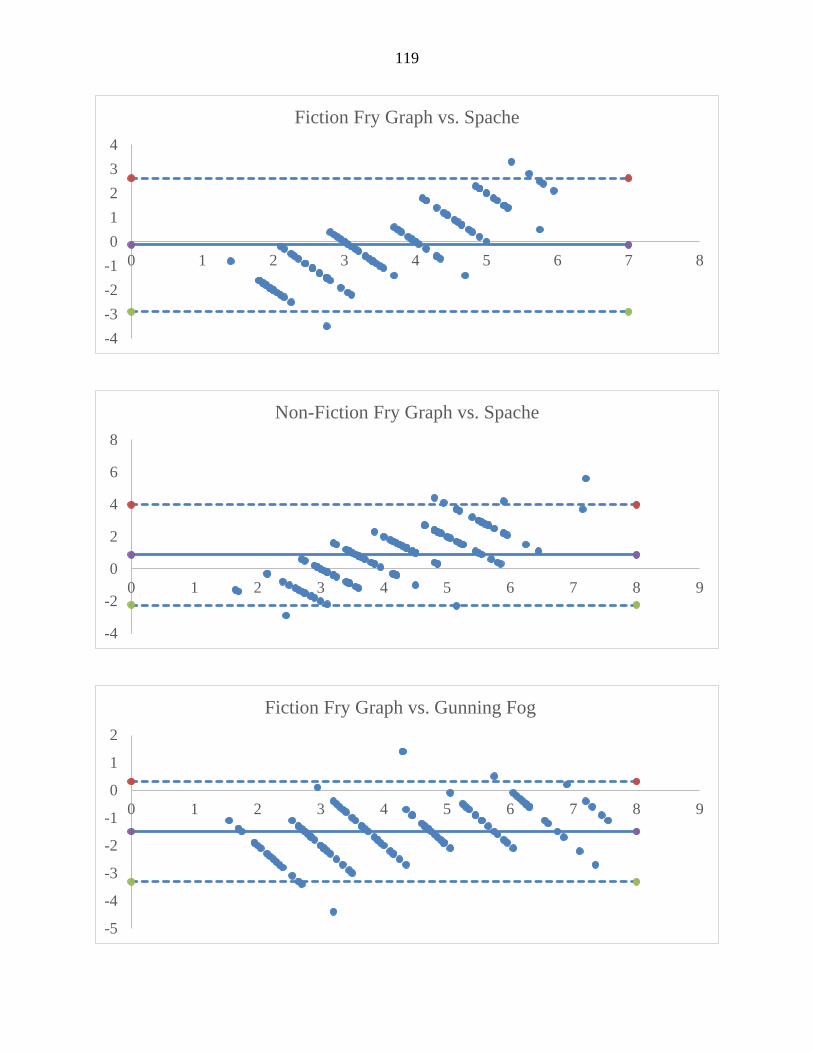
119
-4
-3
-2
-1
0
1
2
3
4
0 1 2 3 4 5 6 7 8
Fiction Fry Graph vs. Spache
-4
-2
0
2
4
6
8
0 1 2 3 4 5 6 7 8 9
Non-Fiction Fry Graph vs. Spache
-5
-4
-3
-2
-1
0
1
2
0 1 2 3 4 5 6 7 8 9
Fiction Fry Graph vs. Gunning Fog

120
-5
-4
-3
-2
-1
0
1
2
0 2 4 6 8 10 12
Non-Fiction Fry Graph vs. Gunning Fog
-4
-3
-2
-1
0
1
2
3
0 1 2 3 4 5 6 7 8 9
Fiction Fry Graph vs. Smog
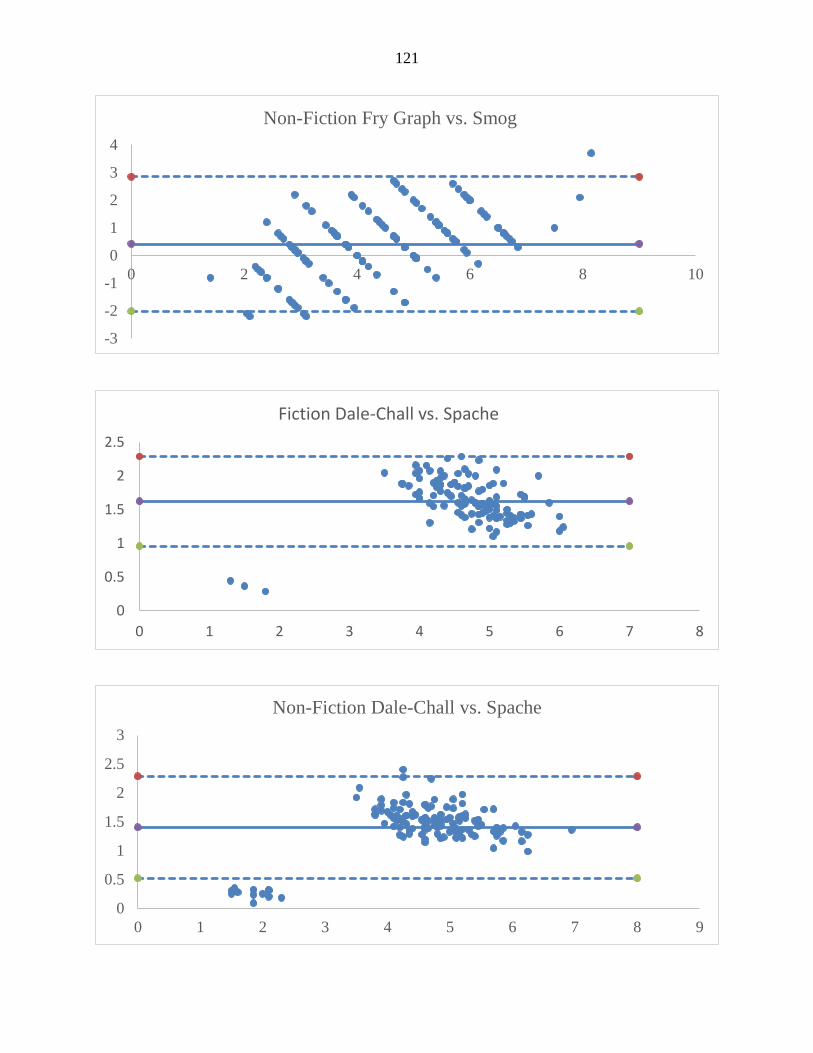
121
-3
-2
-1
0
1
2
3
4
0 2 4 6 8 10
Non-Fiction Fry Graph vs. Smog
0
0.5
1
1.5
2
2.5
0 1 2 3 4 5 6 7 8
Fiction Dale-Chall vs. Spache
0
0.5
1
1.5
2
2.5
3
0 1 2 3 4 5 6 7 8 9
Non-Fiction Dale-Chall vs. Spache

122
-6
-4
-2
0
2
4
6
0 1 2 3 4 5 6 7 8 9
Fiction Dale-Chall vs. Gunning Fog
0
0.5
1
1.5
2
2.5
0 2 4 6 8 10
Non-Fiction Dale-Chall vs. Gunning Fog

123
0
0.5
1
1.5
2
2.5
3
3.5
0 1 2 3 4 5 6 7 8
Fiction Dale-Chall vs. Smog
0
0.5
1
1.5
2
2.5
3
3.5
0 1 2 3 4 5 6 7 8 9
Non-Fiction Dale-Chall vs. Smog
-3
-2
-1
0
1
2
3
0 1 2 3 4 5 6 7
Fiction Spache vs. Smog

124
-5
-4
-3
-2
-1
0
1
2
3
4
0 1 2 3 4 5 6 7 8
Non-Fiction Spache vs. Smog
0
0.5
1
1.5
2
2.5
0 1 2 3 4 5 6 7 8 9
Fiction Gunning Fog vs. Smog

125
REFERENCES
Adams, M. J. (1990). Beginning to Read: Thinking and Learning About Print. Cambridge, MA:
MIT Press.
Allen, D. (2009). A study of the role of relative clauses in the simplification of news texts for
learners of English. System, 37(4), 585-599.
Altman, D. G., & Bland, J. M. (1983). Measurement in medicine: The analysis of method
comparison studies. Statistician, 307-317.
Anderson, R. C., & Pearson, P. D. (1984). A schema-theoretic view of basic processes in
reading. In P. D. Pearson (Ed.), Handbook of Reading Research. White Plains, NY:
Longman.
Ardoin, S. P., Suldo, S. M., Witt, J., Aldrich, S., & McDonald, E. (2005). Accuracy of
readability estimates' predictions of CBM performance. School Psychology Quarterly,
20, 1-22.
Ardoin, S. P., Williams, J. C., Christ, T. J., Klubnik, C., & Wellborn, C. (2010). Examining
readability estimates' predictions of students' oral reading rate: Spache, Lexile, and
Forcast. School Psychology Review, 39, 277-285.
Armbruster, B. B., Lehr, F., & Osborn, J. (2001). Put Reading First: The Reseach Building
Blocks for Teaching Children to Read Kindergarten Through Grade 3. National
Institution of Child Health and Human Development, Partnership for Reading.
Washington, DC: U. S. Department of Education.
Bailin, A., & Grafstein, A. (2001). The linguistic assumptions underlying readability formulae: A
critique. Language and Communications, 21, 285-301.
Baker, L., & Wigfield, A. (1999). Dimensions of children's motivation for reading and their

126
relations to reading activity and reading achievement. Reading Research Quarterly, 34,
452-477.
Begeny, J. C., & Greene, D. J. (2014). Can readability formulas be used to successfully gauge
difficulty of reading materials? Psychology in the Schools, 51(2), 198-215.
Best, R. M., Rowe, M., Ozura, Y., & McNamara, D. S. (2005). Deep-level comprehension of
Science texts: The role of the reader and the text. Top Language Disorders, 25(1), 65-83.
Bland, J. M., & Altman, D. G. (1983). Measurement in medicine: The analysis of method
comparison studies. Statistician, 32, 307-317.
Bland, J., & Altman, D. G. (1999). Measuring Agreement in Method Comparison Studies.
Statistical Methods in Medical Research, 8, 135-160.
Brown, J. D. (1998). An EFL readability index. JALT Journal, 29(2), 7-36.
Burke, V. (2010). Determining Readability: How to select and apply easy-to-use readability
formulas to assess the difficulty of adult literacy materials. Adult Basic Education and
Literacy Journal, 4(1), 34-42.
Carrell, P. (1987). Readability in ESL. REading in a Foreign Language, 4, 21-40.
Chall, J., & Dale, E. (1995). Readability revisited: The new Dale-Chall readability formula.
Cambridge, MA: Brookline Books.
Chhapola, V., Kanwal, S. K., & Brar, R. (2015). Reporting standards for Bland-Altman
agreement analysis in laboratory research: A cross-sectional survey of current practice.
Annals of Clinical Biochemistry, 52(3), 382-386.
Compton, D. L., Appleton, A. C., & Hosp, M. K. (2004). Exploring the relationship between
text-leveling systems and reading accuracy and fluency in second-grade students who are
average to poor decoders. Learning Disabilities Research & Practice, 19, 176-184.

127
Connatser, B. R., & Peac, E. (1999). Last rites for readability formulas in technical
communication. Journal of Technical Writing and Communication, 29, 271-287.
Crossley, S. A., Allen, D. B., & McNamara, D. S. (2011). Text readability and intuitive
simplification: A comparison of readability formulas. Reading in a Foreign Language,
23(1), 84-101.
Crossley, S. A., Greenfield, J., & McNamara, D. S. (2008). Assessing text readability using
cognitively based indices. TESOL Quarterly, 42(3), 475-493.
Dale, E., & Chall, J. (1948). A formula for predicting readability. Educational Research Bulletin,
27, 37-54.
Davison, A., & Kantor, R. N. (1982). On the failure of readability formulas to define readable
texts: A case study from adaptations. Reading Research Quarterly, 17(2), 187-208.
Deci, E., & Ryan, R. (1985). Intrinsic motivation and self-determination in human behavior.
New York, NY: Plenum.
Driscoll, M. P. (2000). Psychology of learning for instruction (2nd ed.). Needham Heights, MA:
Allyn & Bacon.
DuBay, W. (2004). The principles of readability. Retrieved from http://www.impact-
information.com/impactinfo/Resources.htm
Fisher, D., Fray, N., & Lapp, D. (2012). Text complexity: Raising rigor in reading. Newark, DE:
International Reading Association, Inc.
Fitzgerald, G. G. (1980). Reliability of the Fry sampling method. Reading Research Quarterly,
15(4), 489-503.
Flesch, R. (1948). A new readability yardstick. Journal of Applied Psychology, 32, 221-233.
Flesch, R. (1951). How to test readability. New York, NY: Harper and Brothers.

128
Fountas, I. C., & Pinnell, G. S. (2001). Guiding Readers and Writers: Teaching comprehension,
genre, and content literacy. Portsmouth, NH: Heinemann.
Fry. (1968). A readability formula that saves time. Journal of Reading, 11, 513-516.
Fry. (1975). The Readability Principle. Language Arts, 52(6), 847-851.
Gallagher, T. L., Fazio, X., & Gunning, T. G. (2012). Varying readability of science-based text
in elementary readers: Challenges for teachers. Reading Improvement, 93-112.
Gambrell, L. B. (2002). What research reveals about literacy motivation. In P. E. Linder (Ed.),
Celebrating the faces of Literacy (pp. 32-42). Readyville, TN: College Reading
Association.
Gamson, D. A., Lu, X., & Eckert, S. A. (2013). Challenging the research base of the Common
Core State Standards: A historical reanalysis of text complexity. Educational Researcher,
7, 381-391.
Gardner, H. (1987). The mind's new science. New York, NY: Basic Books.
Gernsbacher, M. (1997). Coherence cues mapping during comprehension. In J. &. Costermans
(Ed.), Processing interclausal relationships. Studies in the production and
comprehension of text (pp. 3-22). Mahwah, NJ: Erlbaum.
Giavarina, D. (2015). Understanding the Bland Altman analysis. Biochemica Medica, 25(2),
141-151.
Goldman, S. R., & Rakestraw, J. A. (2000). Structural aspects of constructing meaning from text.
In M. M. Kamil (Ed.), Handbook of reading research (Vol. 3, pp. 311-336). Mahwah,
NJ: Lawrence Erlbaum Associates.
Goldman, S., & Lee, C. (2014). Text complexity: State of the art and the conundrums it raises.
The Elementary School Journal, 115(2), 290-300.

129
Goodman, K. S. (1967). Reading: A psycholinguistic guessing game. Journal of the Reading
Specialist, 6, 126-135.
Graesser, A. C., McNamara, D. D., Louwerse, M. L., & & Cai, Z. (2004). Coh-Metrix: Analysis
of text on cohesion and language. Behavior Research Methods, Instruments, &
Computers, 36, 193-202.
Graesser, McNamara, Louwerse, & Zhiquiang. (2004). Coh-Metrix: Analysis of text on cohesion
and language. Behavior Research Methods, Instruments, & Computers, 36(2), 193-202.
Gunning, R. (1968). The technique of clear writing. New York, NY: McGraw-Hill.
Guthrie, J. T., Hoa, L. W., Wigfield, A., Tonks, S. M., & Perencevich, K. C. (2006). From spark
to fire: Can situational reading interest lead to long-term reading motivation? Reading
Research and Instruction, 45(2), 91-117.
Guthrie, J. T., Hoa, L. W., Wigfield, A., Tonks, S. M., Humenick, N. M., & Littles, E. (2006).
Reading motivation and reading comprehension in later elementary years. Contemporary
Educational Psychology, 32, 282-313.
Guthrie, J. T., Lutz-Klauda, S., & Ho, A. N. (2013). Modeling the relationships among reading
instruction, motivation, engagement, and achievement for adolescents. Reading Research
Quarterly, 48(1), 9-26.
Guthrie, J. T., Wigfield, A., Metsala, J. L., & Cox, K. E. (1999). Motivational and cognitive
predictors of text comprehension and reading amount. Scientific Studies of Reading, 3(3),
231-256.
Hanneman, S. K. (2008). Design, Analysis and Interpretation of Method-Comparison Studies.
AACN Advanced Critical Care, 19(2), 223-234.
doi:10.1097/01.AACN.0000318125.41512.a3
130
Harrison. (1980). Readability in the classroom. New York, NY: Cambridge University.
Harvey, S., & Goudvis, A. (2000). Strategies That Work. Portland, Maine: Stenhouse Publishers.
Hauptli, M. V., & Cohen-Vogel, L. (2013). The federal role in adolescent literacy from Johnson
through Obama: A policy regime analysis. American Journal of Education, 119(3), 373-
404.
Hiebert, E. H., & Mesmer, H. E. (2013). Upping the ante of text complexity in the Common
Core State Standards: Examining its potential on young readers. Educational Researcher,
42(1), 44-51.
Hintze, J. M., & Christ, T. J. (2004). An examination of variability as a function of passage
variance in CBM progress monitoring. School Psychology Review, 33, 204-217.
Hittleman, D. R. (1973). Seeking a Psycholinguistic Definition of Readability. The Reading
Teacher, 26(8), 783-789.
Johnson, D. (1971). The Dolch list re-examined. The Reading Teacher, 24, 449-457.
Just, M. A., & Carpenter, P. A. (1987). The psychology of reading and language comprehension.
Boston, MA: Allyn & Bacon, Inc.
Klare, G. R. (1963). The measurement of readability. Ames, IA: Iowa State University Press.
Klare, G. R. (1974-1975). Assessing readability. Reading Research Quarterly, 10, 62-102.
Klare, G. R. (1984). Readability. In P. D. Pearson (Ed.), Handbook of reading reserach (pp. 681-
744). New York: Longman.
Koda, K. (2005). Insights into second language reading. Cambridge, MA: Cambridge University
Press.
Kuhn, M., & Stahl, S. (2013). Fluency: A review of developmental and remedial practices.
Journal of Educational Psychology, 95, 3-21.

131
Lively, B., & Pressley, S. (1923). A method for measuring the "vocabulary burden" of textbooks.
Educational Administration and Supervision, 99, 389-398.
Logan, S., Medford, E., & Hughes, N. (2011). The importance of intrinsic motivation for high
and low level ability readers' reading comprehension performance. learning and
Individual Differences, 21, 124-128.
Ludbrook, J. (2010). Confidence in Altman-Bland plots: A critical review of the method of
differences. Clinical and Experimental Pharmacology and Physiology, 37, 143-149.
McGeown, S. P., Norgate, R., & Warhurst, A. (2012). Exploring intrinsic and extrinsic reading
motivation among very good and very poor readers. Educational Research, 54(3), 309-
322.
McLaughlin. (1969). SMOG grading-a new readability formula. Journal of Reading, 22, 639-
646.
McLaughlin. (1975). Evaluation and Reform. Cambridge, MA: Ballinger.
McNamara, D. S., Kintsch, E., Butler-Song, N., & Kintsch, W. (1996). Are good texts always
better? Interactions of text coherence, background knowledge, and levels of
understanding in learning from text. Cognition and Instruction, 14, 1-43.
Mesmer, H. A., Cunningham, J. W., & Hiebert, E. H. (2012). Toward a theoretical model of text
complexity for the early grades: Learning from the past, anticipating the future. Reading
Research Quarterly, 47, 235-258.
Meyer, B. J. (1984). Text dimensions and cognitive processing. In H. S. Mandl (Ed.), Analyzing
and understanding expository text (pp. 3-47). Hillsdale, NJ: Erlbaum.
Meyer, B. J. (2003). Text coherence and readability. Top Language Disorders, 23(3), 204-224.
Mikk, J. (2001). Prior knowledge of text content and values of text characteristics. Journal of

132
Quantitative Linguistics, 8(1), 67-80.
Moen, E. (2016). Objective statistics for the measurement of agreement (Unpublished doctoral
disseration). Wayne State University, Detroit, MI.
Moley, P. F., Bandre, P. E., & George, J. E. (2011). Moving beyond readability: Considering
choice, motivation, and learner engagement. Theory Into Practice, 50, 247-253.
Morrow, L. M. (2011). Literacy Development in the Early Years: Helping Children Read and
Write (4th ed.). Boston, MA: Allyn and Bacon.
Myles, P. S., & Cui, J. (2007). Using Bland-Altman method to measure agreement with repeated
measures. British Journal of Anaesthesia, 99(3), 309-311.
National Governors Association Center for Best Practices & Council of Chief State School
Officers [NGA & CCSSO]. (2010). Common Core State Standards: English Language
Arts. Washington, DC: National Governors Association for Best Practices and Council of
Chief State School Officers.
Papola-Ellis, A. (2014). Text complexity: The importance of building the right staircase. Reading
Horizons, 53(2), 1-27.
Pearson, P. D. (2013). Research foundations for the Common Core Standards in English
language arts. In S. Neuman (Ed.), Quality reading instruction in the age of the Common
Core State Standards. Newark, DE: International Reading Association.
Pearson, P. D., & Hiebert, E. (2014). The state of the field: Qualitative analyses of text
complexity. The Elementary School Journal, 115(2), 161-183.
Pearson, P. D., & Hiebert, E. (2014). Understanding Text Complexity: Introduction to the
Special Issue. The Elementary School Journal, 115(2), 153-160.
Pearson, P. D., Hiebert, E., & Kamil, M. L. (2007). Vocabulary assessment: What we know and

133
what we need to learn. Reading Research Quarterly, 42(2), 282-296.
Perfetti, C. A. (1985). Reading ability. Oxford: Oxford University Press.
Plucinski, K. J. (2010). Readability of intermediate accounting textbooks. Academy of
Educational Leadership Journal, 14(2), 49-57.
Reed, D. K., & Kershaw-Herrara, S. (2016). An examination of text complexity as characterized
by readability and cohesion. The Journal of Experimenal Education, 1, 75-97.
Ricker, K. S. (1978). But can they read it? A look at readability formulas. Science Teacher, 3,
22-24.
Roller, B., Eller, W., & Chapman, C. (1980). NAEP Reading Assessment. The Reading Teacher,
33(8), 938-940.
Rush, R. T. (1985). Assessing readability: Formulas and alternatives. The Reading Teacher,
39(3), 274-283.
Shanahan, T., Fisher, D., & Fray, N. (2012). The challenge of challenging text. Educational
Leadership, 69(6), 58-62.
Shymansky, J. A., & Yore, L. D. (1979). Assessing and Using Readability of Elementary
Science Texts. School Science and Mathematics, 670-676.
Snow, C. E., & Sweet, A. P. (2003). Reading for comprehension. In C. Snow, & A. Sweet (Eds.),
Rethinking reading comprehension (pp. 1-11). New York, NY: Guilford Press.
Snow, C. E., Burns, M. S., & Griffin, P. (1998). Preventing Reading Difficulties in Young
Children. Washington, DC: National Academy Press.
Spache, G. (1953). A new readability formula for primary-grade reading materials. Elementary
School Journal, 53, 410-413.
Stahl, S. A. (2003). Vocabulary and readability: How knowing word meanings affects
134
comprehension. Top Language Disorders, 23(3), 241-247.
Stevens, N. T., Steiner, S. H., & MacKay, R. J. (2015). Assessing agreement between two
measurement systems: An alternative to the limits of agreement approach. Statistical
Methods in Medical Research, 1-22.
Thorndike, R. L. (1972). Reading as reasoning. Reading Research Quarterly, 9, 135-147.
Wang, J. H., & Guthrie, J. T. (2004). Modeling the effects of intrinsic motivation, extrinsic
motivation, amount of reading, and past reading achievement on text comprehension
between U.S. and Chinese students. Reading Research Quarterly, 39, 162-186.
Wray, D., & Janan, D. (2013). Readability revisited? The implications of text complexity. The
Curriculum Journal, 24(4), 553-562.
Zakaluk, B. L., & Samuels, S. (1988). Readability: Its past, present, & future. Newark, DE:
International Reading Association.
Zimmerman, S., & Hutchins, C. (2003). 7 Keys to Comprehension: How to help your kids read it
and get it! New York, NY: Three Rivers Press.

135
ABSTRACT
COMPARISON OF READABILITY INDICES WITH GRADES 1-5 NARRATIVE AND
EXPOSITORY TEXTS
by
SUSAN HARDEN
December 2018
Advisor: Dr. Shlomo Sawilowsky
Major: Education Evaluation and Research
Degree: Doctor of Philosophy
The problem that exists when using one or more readability indexes to ascertain a text
grade level is the varied outcomes received on any given text from readability indexes that purport
to measure the same construct. This study aims to provide practitioners with data to make informed
decisions regarding interchangeability of readability indexes. A total of n = 244 narrative (n = 116)
and expository texts (n = 128) passages from grades 1-5 were evaluated using the following
readability indexes: Flesch-Kincaid Grade Level, Fry Graph, Spache, Dale-Chall, Gunning Fog,
and Smog. Fifteen (15) comparison sets were analyzed using Bland-Altman method to assess for
agreement. An a priori set standard of 1.5 grade levels was used as an acceptable difference. Other
considerations for agreement included narrow limits of agreement, low proportional error, and a
Bland-Altman plot where data points clustered around the bias line. Of the fifteen (15) comparison
sets, nine (9) resulted in agreement, or near agreement. Based on the findings of the study and the
subjectivity of the Bland-Altman method, it is recommended that practitioners select one
readability index for text evaluation and use it exclusively. No particular index was recommended
for use. The use of readability indexes should be one of several means of evaluating a text.

136
AUTOBIOGRAPHICAL STATEMENT
Susan Harden was born April 28, 1972 in East Grand Rapids, Michigan. She grew up in
Rochester Hills, MI where she graduated from Rochester High School in 1990. Following high
school Susan spent two years at Michigan State University before transferring to Oakland
University where she earned her Bachelor of Science in Elementary Education with a major in
mathematics in 1996. She continued on at Oakland University to earn a Master of Arts in Teaching
Reading and Language Arts in 2004.
Susan is currently certified to teach all subjects at the elementary grades K-5, Mathematics
grades K-8, and is a certified Reading Specialist.
Previously, Susan has taught in the Birmingham Public Schools (Michigan) and the
Livonia Public Schools (Michigan). She has also served as an educational consultant with Wayne
RESA High Priority Schools in Detroit, MI in the realm of English/Language Arts.