comparison of two approaches for determining ground-water
TRANSCRIPT

U.S. GEOLOGICAL SURVEY
Water-Resources Investigations Report 99–4221
Comparison of Two Approaches forDetermining Ground-Water Dischargeand Pumpage in the Lower ArkansasRiver Basin, Colorado, 1997–98
By Russell G. Dash, Brent M. Troutman, and Patrick Edelmann
Denver, Colorado1999
Prepared in cooperation with theCOLORADO DEPARTMENT OF NATURAL RESOURCES,DIVISION OF WATER RESOURCES,OFFICE OF THE STATE ENGINEER

U.S. DEPARTMENT OF THE INTERIORBRUCE BABBITT, Secretary
U.S. GEOLOGICAL SURVEY
Charles G. Groat, Director
The use of firm, trade, and brand names in this report is for identification purposes only and doesnot constitute endorsement by the U.S. Geological Survey.
For additional information write to: Copies of this report can be purchased
U.S. Geological SurveyInformation ServicesBox 25286Federal CenterDenver, CO 80225
from:
District ChiefU.S. Geological SurveyBox 25046, Mail Stop 415Denver Federal CenterDenver, CO 80225–0046
CONTENTS
5
.
89
..
13
.. 15
..... 22
....... 23
...... 24
.. 27
28
Executive Summary ............................................................................................................................................................... 1Introduction............................................................................................................................................................................
Purpose and Scope....................................................................................................................................................... 5Acknowledgments ....................................................................................................................................................... 6
Methods of Investigation ....................................................................................................................................................... 6Totalizing Flowmeter Measurements........................................................................................................................... 7Portable Flowmeter Measurements ............................................................................................................................. 8Power Conversion Calculations and Computations of Pumpage................................................................................. 9Quality Control of Data ............................................................................................................................................... 10Overview of the Statistics Used for Comparing Discharge and Pumpage ................................................................. 10
Comparison of Instantaneous Ground-Water Discharge Measurements ............................................................................... 11Primary Results............................................................................................................................................................ 12Details of Analysis and Results ................................................................................................................................... 12
Temporal Variations in Power Conversion Coefficients ........................................................................................................ 19Short-Term Variations in Power Conversion Coefficients ........................................................................................... 19Long-Term Variations in Power Conversion Coefficients ........................................................................................... 21
Comparison of Ground-Water Pumpage Estimates ............................................................................................................... 25Primary Results............................................................................................................................................................ 25Details of Analysis and Results ................................................................................................................................... 25
Sources of Discrepancy Between Pumpage Estimates .......................................................................................................... 30Primary Results............................................................................................................................................................ 30Details of Analysis and Results ................................................................................................................................... 31
Estimation of Total Network Pumpage.................................................................................................................................. 33Primary Results............................................................................................................................................................ 33Details of Analysis and Results ................................................................................................................................... 34
Conclusions............................................................................................................................................................................ 3References Cited.................................................................................................................................................................... 3
FIGURES
1. Map showing location of study area and irrigation-wells used in the study, 1997–98 ............................................. 22. Graphs showing relation of instantaneous discharge measurements from totalizing flowmeter to the
differences in instantaneous discharge measurements between portable flowmeters and totalizingflowmeters, expressed (A) in logarithmic units and (B) in gallons per minute ...........................................................
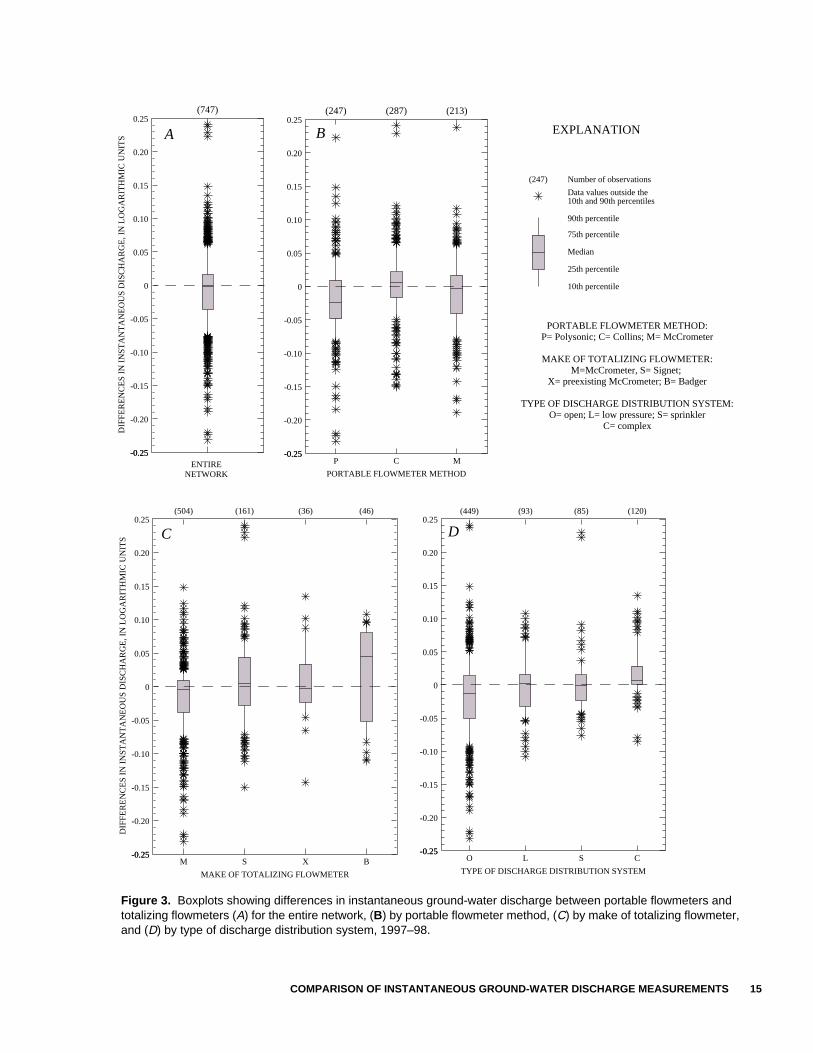
3. Boxplots showing differences in instantaneous ground-water discharge between portable flowmetersand totalizing flowmeters (A) for the entire network, (B) by portable flowmeter method, (C) by makeof totalizing flowmeter, and (D) by type of discharge distribution system, 1997–98...............................................
4–9. Graphs showing:4. Distribution of differences in instantaneous ground-water discharge between portable flowmeters
and totalizing flowmeters for network sites during 1998................................................................................... 165. Power conversion coefficients (PCC) determined at network sites during 1998: (A) range in PCC
and (B) percent difference .................................................................................................................................. 206. Seasonal distribution of power conversion coefficients (PCC) for network sites during 1998.....................7. Power conversion coefficients (PCC) determined at selected network sites during 1997 and 1998...........8. Power conversion coefficients (PCC) at network sites: (A) 1994–97 State-approved PCC and 1998
PCC, and (B) percent difference between 1994–97 State-approved PCC and 1998 PCC ...........................9. Relation of ground-water pumpage from inline totalizing flowmeter to the differences in pumpage
estimates between power conversion coefficient approach and totalizing flowmeters, expressed(A) in logarithmic units and (B) in acre-feet ....................................................................................................
10. Boxplots showing differences in ground-water pumpage estimates between power conversion coefficientapproach and totalizing flowmeters (A) for the entire network, (B) by portable flowmeter method,(C) by make of totalizing flowmeter, and (D) by type of discharge distribution system, 1998..................................
11. Graph showing relation of the mean and standard deviation of total network pumpage, in percent,to the number of strata ................................................................................................................................................ 37
CONTENTS III

...... 17
....
..... 18......... 19
.....
....
TABLES
1. Estimates of mean differences in instantaneous ground-water discharge between portable flowmetersand totalizing flowmeters for the grand mean and fixed effects of method, make, and type ............................
2. Estimates of mean differences in instantaneous ground-water discharge between portable flowmetersand totalizing flowmeters among fixed effects of method, make, and type ........................................................ 18
3. Estimates of mean differences in instantaneous ground-water discharge between portable flowmetersand totalizing flowmeters for each combination of fixed effects of method, make, and type............................
4. Estimates of the variances of the site, date, and error random terms in discharge measurements.................5. Comparison of State-approved power conversion coefficient (PCC) measurements (1994–97) to the
site average PCC measurements made during 1998 ............................................................................................... 256. Estimates of mean differences in pumpage between power conversion coefficient approach and totalizing
flowmeter for the grand mean and fixed effects of method, make, and type ..................................................... 297. Estimates of mean differences in pumpage between power conversion coefficient approach and totalizing
flowmeter among fixed effects of method, make, and type..................................................................................... 298. Estimates of mean differences in pumpage between power conversion coefficient approach and totalizing
flowmeter for each combination of fixed effects of method, make, and type ..................................................... 30
CONVERSION FACTORS AND ABBREVIATIONS
The following terms and abbreviations are used in this report:
Power Conversion Coefficient (PCC)Totalizing Flowmeter (TFM)Colorado Division of Water Resources (CDWR)U.S. Geological Survey (USGS)
Method of Portable Flowmeter:
C (Collins flowmeter)M (McCrometer flowmeter)P (Polysonic flowmeter)
Make of Inline Totalizing Flowmeter:
M (new McCrometer TFM)S (new Signet TFM)X (existing McCrometer TFM)B (existing Badger TFM)R (existing Rockwell TFM)
Type of Discharge Distribution System:
O (open)L (low-pressure)S (sprinkler)C (complex)
Multiply By To obtain
acre-foot (acre-ft) 1,233 cubic meter
foot (ft) 0.3048 meter
gallons per minute (gal/min) 0.00379 cubic meter per minute
inch (in.) 2.54 centimeter
kilowatthour (kWh) 3,600,000 joule
kilowatthour per acre-foot 2,919 joule per cubic meter
IV CONTENTS

tefirst,ofn
he
ing
f ther toer data
earingpact
liability
ares. The
tate line
r morees and at afficient
Comparison of Two Approaches for DeterminingGround-Water Discharge and Pumpage in theLower Arkansas River Basin, Colorado, 1997–98By Russell G. Dash, Brent M. Troutman, and Patrick Edelmann
Several sections of this report contain detailed mathematical derivations and statistics. To facilitareading and use of this report, the report is organized in a manner that presents the primary resultsthen the detailed mathematical derivations and statistics in the sections that follow titled “Details Analysis and Results”. For those readers who are interested only in the primary results, rather thathe derivations and details, they may wish to read the sections titled “Primary Results” and skip tsections titled “Details of Analysis and Results”.
EXECUTIVE SUMMARY
Introduction
In March 1994, the Colorado Division of Water Resources (CDWR) adopted “Rules Governthe Measurement of Tributary Ground Water Diversions Located in the Arkansas River Basin”(Office of the State Engineer, 1994); these initial rules were amended in February 1996 (Office oState Engineer, 1996). The amended rules require users of wells that divert tributary ground wateannually report the water pumped monthly by each well. The rules allow a well owner to report thpumpage measured by a totalizing flowmeter (TFM) or pumpage determined from electrical poweand a power conversion coefficient (PCC) (Hurr and Litke, 1989).
Opinions by representatives of the State of Kansas, presented before the Special Master ha court case [State of Kansas v. State of Colorado, No. 105 Original (1996)] concerning post-Comwell pumping, stated that the PCC approach does not provide the same level of accuracy and reas a TFM when used to determine pumpage.
In 1997, the U.S. Geological Survey (USGS), in cooperation with the CDWR, began a 2-yestudy to compare ground-water pumpage estimates made using the TFM and the PCC approachstudy area was along the Arkansas River between Pueblo, Colorado, and the Colorado-Kansas S(fig. 1).
The two approaches for estimating ground-water discharge and pumpage were compared fothan 100 wells completed in the alluvial aquifer of the Arkansas River Basin. The TFM approach usinline flowmeter to directly measure instantaneous discharge and the total volume of water pumpewell. The PCC approach uses electrical power consumption records and a power conversion coeto estimate the pumpage at ground-water wells.
EXECUTIVE SUMMARY 1

ecifi-
s PCC’statisticalepancythe two
er theta thattotal
thestanta-. The
C O L O R A D O
Denver
PuebloCounty
Crowley
OteroCounty Bent
County
Prowers
Study Area
La Junta Las Animas
Pueblo
EXPLANATION
Irrigation well CO
LO
RA
DO
KA
NS
AS
Lamar
John Martin Res.
ARKANSASRIVER
Foun
tain
Cr
Huer
fano R
Api
sha p
aR
Purgat
oir
eR
Two B utte
sC
r
County
County
Figure 1. Map showing location of study area and irrigation-wells used in the study, 1997–98.
This executive summary describes the results of the comparison of the two approaches. Spcally, (1) the differences in instantaneous discharge measured with three portable flowmeters andmeasured with an inline TFM are evaluated, and the statistical differences in paired instantaneoudischarge between the two approaches are determined; (2) short- and long-term variations in theare presented; (3) differences in pumpage between the two approaches are evaluated, and the sdifferences in pumpage between the two approaches are determined; (4) potential sources of discrbetween pumpage estimates are discussed; and (5) differences in total network pumpage using approaches are presented.
During the irrigation seasons of 1997 and 1998, instantaneous discharge and electrical powdemand were measured at randomly selected wells to determine PCC’s. At more than 100 wells,PCC’s determined during the 1998 season were applied to total electrical power consumption dawas recorded between the initial and final readings at each network well site in 1998 to estimate ground-water pumpage.
At each site, an inline TFM was installed in a full-flowing, acceptable test section of pipe ondischarge side of the pump where the measurement of discharge was made. Measurements of inneous ground-water discharge also were made using three different types of portable flowmeters
2 Comparison of Two Approaches for Determining Ground-Water Discharge and Pumpage in theLower Arkansas River Basin, Colorado, 1997–98

e each
eous05 wellsasnd entire
were
hanr the
compar-utent ofrements
ured bya siteed PCC
About
M andPCC.
ithin-at the
average velocity multiplied by the cross-sectional area of the discharge pipe was used to computthe discharge in gallons per minute. Whenever possible, discharge measurements were made atnetwork site using all three types of portable flowmeters.
Comparison of Instantaneous Ground-Water Discharge Measurements
Instantaneous discharges measured using portable flowmeters were compared to instantandischarges measured using TFM’s. The analysis is based on 747 paired measurements taken at 1during a 2-year period. A mixed analysis of variance model with both fixed and random effects wapplied. The overall mean difference in discharge measurements between portable flowmeters aTFM’s was 0.00 percent, indicating no difference on average between the two approaches for thenetwork of wells. More than 80 percent of the differences in the paired discharge measurementsless than 10 percent.
Temporal Variations in Power Conversion Coefficients
Analysis of variations in PCC’s measured during the 1998 irrigation season indicated that58 percent of 104 wells had less than 10-percent change, and 86 percent of 104 wells had less t20-percent change in the well PCC’s. Seasonal variations in PCC’s generally were not evident fomeasurements made during the 1998 irrigation season. Thirty-seven of the 41 wells with PCC’smeasurements in 1997 had at least one PCC in the same range as 1998 PCC measurements. Theison of the 2 years of data indicate that PCC measurements were similar in 1997 and 1998. Abo48 percent of available pre-study State-approved PCC’s made during 1994–97 were within 10 percthe 1998 site average PCC’s, and about 67 percent of the pre-study State-approved PCC measumade during 1994–97 were within 20 percent of the 1998 site average PCC’s.
Comparison of Ground-Water Pumpage Estimates
Pumpage estimates computed using the PCC approach were compared to pumpage measa TFM at network wells. PCC pumpages were computed by applying each PCC obtained during visit in 1998 to the total 1998 electrical power consumption. The analysis was based on 553 pairpumpage estimates at 103 wells. The overall mean difference in pumpage between the TFM andapproach was 0.01 percent for the entire network of wells, indicating no significant difference onaverage between pumpage measured by a TFM and pumpage computed by the PCC approach.80 percent of the differences in the paired pumpage estimates were less than 10 percent.
Sources of Discrepancy Between Pumpage Estimates
There are several potential sources of discrepancy between pumpage as measured by a TFpumpage as computed by the PCC approach. One potential source is temporal variability of the The analysis indicated that the year-to-year variance component was about nine times the date-wyear variance component and represented a standard deviation of about 15 percent, indicating thyear-to-year variability was a major component of overall variability for this PCC data set.
EXECUTIVE SUMMARY 3

idinge.ther
abilityweenuld be
Estimation of Total Network Pumpage
Differences in the total or aggregated pumpage for a network of wells was estimated by divthe range of TFM pumpage into equal subdivisions based on the magnitude of TFM total pumpagBecause the correct number of subdivisions (strata) is not known with information now available, mean and standard deviation of differences in the total pumpage was determined conditionally foseveral numbers of strata. For a network of 103 wells and a number of strata greater than 10, theresulting mean and standard deviation indicates that, for any given year, there is a 95-percent probthat the difference in aggregated pumpage between the TFM and PCC approaches would be betabout−3.41 and 1.59 percent. The analysis indicates that the difference in aggregated pumpage woexpected to be smaller as the total number of wells becomes larger.
4 Comparison of Two Approaches for Determining Ground-Water Discharge and Pumpage in theLower Arkansas River Basin, Colorado, 1997–98

a-
oing
).
s,
en
y
n
INTRODUCTION
Irrigation is the largest use of water in south-eastern Colorado, and ground water is a supplementalsource for irrigators in the Arkansas River Basinbecause surface-water supplies in the basin are inade-quate to meet irrigation demand. During the past40 years, ground-water withdrawals were occasionallymeasured (Luckey, 1972) but were not routinelymetered. Some estimates of ground-water withdrawalswere reported (Litke and Appel, 1989). However, theaccuracy of the ground-water withdrawal estimateswere not known.
In March 1994, the Colorado Division of WaterResources (CDWR) adopted “Rules Governing theMeasurement of Tributary Ground Water DiversionsLocated in the Arkansas River Basin” (Office of theState Engineer, 1994); these initial measurement ruleswere amended in February 1996 (Office of the StateEngineer, 1996). The “Amendments to RulesGoverning the Measurement of Tributary GroundWater Diversions Located in the Arkansas RiverBasin” were approved in June 1996 and require thatabout 1,600 wells that divert tributary ground watermust annually report the water pumped monthly byeach well. The rules allow a well owner the option ofreporting pumpage measured by a totalizing flowmeter(TFM) or estimated using electrical power consump-tion data and a power conversion coefficient (PCC)(Hurr and Litke, 1989). The inline TFM and the PCCrating must be checked at least once every 4 years by aperson approved by the State Engineer. A TFM is aninline flowmeter that directly measures the totalvolume of water pumped from the well. The PCCapproach uses measurements of instantaneous ground-water discharge, hereinafter referred as instantaneousdischarge, and instantaneous electrical power demand,hereinafter referred as power demand, to determinethe number of kilowatthours of energy required topump 1 acre-foot of water. Since 1994 when the rulesbecame effective in the river basin, most well ownershave chosen to use the PCC approach to determineground-water pumpage from their irrigation wells.
Opinions by representatives of the State ofKansas, presented before the Special Master of theU.S. Supreme Court hearing a case (State of Kansas v.State of Colorado, No. 105 Original (1996))concerning well pumping after approval of theArkansas River Compact of 1948, stated that the PCCapproach does not provide the same level of accuracy
and reliability as the TFM’s when used to determineannual ground-water pumpage. Thereafter, theColorado State Engineer proposed a study to deter-mine the comparability of estimates of ground-waterpumpage using the TFM and PCC approaches. In1997, the U.S. Geological Survey (USGS), in coopertion with the Colorado Department of NaturalResources, Division of Water Resources, Office ofthe State Engineer (CDWR), began a 2-year study tcompare ground-water pumpage estimates made usthe TFM and PCC approaches. The study area wasthe Arkansas River alluvial valley between Pueblo,Colorado, and the Colorado-Kansas State line (fig. 1
Purpose and Scope
This report provides a comparison of twoapproaches for determining ground-water dischargeand pumpage. Specifically, this report:
1. Evaluates differences in instantaneous dischargebetween TFM’s and three portable flowmetersused with the PCC approach, and determinesif differences in instantaneous discharge forthe TFM and PCC approach are statisticallysignificant;
2. Evaluates short- and long-term variations in PCC’including whether seasonal variations in PCC’swere evident;
3. Evaluates differences in ground-water pumpageestimated with the TFM and PCC approaches,and determines if differences in ground-waterpumpage estimated with the TFM and PCCapproaches are statistically significant;
4. Evaluates potential sources of discrepancy betwepumpage estimates; and
5. Estimates differences in total network pumpageusing the two approaches.
One hundred and six irrigation wells that arepowered by electric pumps were selected for this studfrom about 1,300 irrigation wells in the study area.The network of 106 irrigation wells consisted of11 wells that had TFM’s installed prior to the studyand 95 randomly selected wells that had new TFM’sinstalled during 1997–98. During the irrigation seasoof 1997, instantaneous discharge was measured at46 wells (43 of which had TFM’s in 1997) and, during1998, at 105 wells. One irrigation well was droppedfrom the network following the 1997 irrigation season
INTRODUCTION 5

-
hef
ed
n
l
oes
d
des-
,
m
,ll
because the well owner had reconfigured the dischargedistribution system and combined the plumbing of twowells together. This activity created a complex wellthat was not suitable under the amended rules forRule 3.6 analyses (Office of the State Engineer, 1996),making the well unacceptable for the continued appli-cation of a PCC to determine ground-water pumpage.
During the study, PCC’s were calculated eachtime a portable flowmeter measurement of the instan-taneous discharge and power demand were made at awell. At 104 of the wells, PCC’s determined during the1998 irrigation season were applied to the total elec-trical power consumption recorded between the initialand final readings at the site in 1998 to estimate totalground-water pumpage for the period. The totalpumpage estimate derived using the PCC calculationthen was compared to the total pumpage measuredusing the TFM at 104 wells. However, pumpage datafrom one well were omitted because it was determinedthat the existing TFM (make R) was not working prop-erly, which resulted in 103 wells that were used forcomparison of ground-water pumpage.
Acknowledgments
The authors wish to thank the CDWR personnel,specifically, Keith Kepler P.E., G.R. Barta P.E., D.G.(Dan) DiRezza, W.A. (Bill) Richie, W.W. (Bill) Tyner,and R.L. (Bob) Plese, Jr., who obtained well-ownerpermissions, arranged the purchase and installation ofTFM’s, measured instantaneous discharges, providedelectrical power consumption records, recorded fieldmeasurements, and provided the USGS with electronicdata that were used for this study. Without their dedi-cated work, the study could not have been completed.The authors acknowledge the support of the ColoradoWater Conservation Board, and in particular SteveMiller. The authors also appreciate the cooperationof many private landowners in the basin who allowedtheir irrigation wells to be used in this study.
METHODS OF INVESTIGATION
Data collection and analysis consisted of severalphases: (1) Identification of potential sites; (2) selec-tion of sites for TFM/PCC comparisons; (3) installa-tion of the TFM’s; (4) measurement of instantaneous
discharges; (5) determination of PCC’s; (6) computation of ground-water pumpage using TFM and PCCapproaches; and (7) analysis of data.
Initially, the CDWR identified more than1,300 large-capacity irrigation wells (wells thatdischarge more than 50 gal/min) in the ArkansasRiver Valley between Pueblo, Colorado, and theColorado-Kansas State line for which the PCCapproach might be used to determine ground-waterpumpage under the amended rules established by tOffice of the State Engineer (1996). This initial list owells was decreased to about 800 potential sites forTFM/PCC consideration based on the followingcriteria:
1. The well was reported as active and was connectto a power source.
2. The well used an electric motor, as opposed to ainternal combustion engine.
3. The well had at least 10 acre-ft of reported annuapumpage at least once since 1994.
A computer program (Scott, 1990) was used trandomly select one primary and four alternative sitfor each potential well in the TFM/PCC network. Eachprimary site was evaluated by CDWR and inventorieto determine its suitability for inclusion in theTFM/PCC study. If a primary site was rejected, arandomly selected alternative site was evaluated anso on down the list of alternatives until a suitable sitwas found. During 1997, CDWR evaluated 107 wellfor potential TFM installation; in 1998, CDWR evaluated 122 wells for additional TFM installations. Themost common reasons for rejection and the totalnumber of well sites rejected during 1997–98 wereas follows:
1. The site was determined to be a complex systemand was found unsuitable for Rule 3.6 analysesor the site was determined to be a compoundsystem, or the owner indicated future modifica-tions were planned that would make the siteunsuitable for continued application of the PCCapproach. Compound system means that morethan one electrical device is being operated frothe same electrical power meter. (38 wellsrejected)
2. The discharge pipe was in poor physical conditionthe pump surged or was unable to maintain a fupipeline of flow at a measurement section, or
6 Comparison of Two Approaches for Determining Ground-Water Discharge and Pumpage in theLower Arkansas River Basin, Colorado, 1997–98

of
e
-
d
at
y
,
f
ter-
e
t.
,
there was inadequate upstream or downstreamdistances available to correctly install a TFM.(32 wells rejected)
3. The well owner declined to participate in theTFM/PCC study. (19 wells rejected)
4. The well had less than 10 acre-ft of pumpagereported the previous year. (12 wells rejected)
5. The well appeared to be inactive, and the ownerindicated it was not used. (9 wells rejected)
6. The discharge pipe was not a correct size for instal-lation of a Signet TFM (one of the brands ofTFM used in the study). Pipe was smaller than8-inch diameter during 1997, or smaller than6-inch diameter during 1998, or was larger than12-inch diameter during either year. (24 wellsrejected)
In 1997, permission to measure discharge at46 wells was obtained, including 11 wells that hadpre-existing TFM’s and 35 wells where new TFM’swere planned to be installed during the 1997 irrigationseason. During 1997, discharge measurements ofinstalled TFM’s were made at 43 of the 46 wells in themonitoring network. One new TFM was not installeduntil the end of the 1997 irrigation season, and two ofthe new TFM’s were returned to the factory for cali-bration and were not reinstalled until after the 1997irrigation season. One pre-existing TFM well wasreconfigured to a complex system after the 1997 irri-gation season and was dropped from the study. During1998, permission to install TFM’s and measuredischarge at 60 additional wells was obtained. Thechanges resulted in a final monitoring network of105 wells having TFM’s. However, upon evaluationof the data, an electric power meter at one site wasfound to be malfunctioning, resulting in 104 wellsbeing used for analysis of variations in PCC’s; and aTFM was found to be malfunctioning at another site,resulting in 103 wells being used to compare ground-water pumpage.
Each well in the network was visited to identifydischarge system characteristics and to confirm thatthe PCC approach could be properly applied at thewell in accordance with the amended rules (Officeof the State Engineer, 1996). When possible, wellowners and operators were interviewed and informa-tion was collected about normal operating conditions,flow ranges and pressures, and number of discharge
distribution outlet locations. Well-identifying datawere recorded from the motor, pump, and electricalmeter nameplates during the visit.
The CDWR made an onsite identification of thetype of discharge distribution system at each of thewells in the network, based on a visual observation the discharge plumbing during the initial visit, whichwas confirmed before making subsequent fieldmeasurements. For this study, four major types ofdischarge distribution systems were identified. Thewell network included 65 open-discharge, 18 low-pressure, 10 sprinkler, and 12 complex dischargedistribution systems. Hereinafter, the open-dischargdistribution system type is referred to as type O, thelow-pressure discharge distribution system type isreferred to as type L, the sprinkler discharge distribution system type is referred to as type S, and thecomplex discharge distribution system type is referreto as type C.
According to the CDWR, well sites that areclassified as complex systems will vary the totaldynamic head (TDH) at the pump during the irrigationseason. The change in TDH may result from wells thdischarge into a pipeline with multiple outlet loca-tions, multiple wells that discharge into one commonpipeline, or wells where the method of water deliverchanges between different types of distributionsystems, such as open-discharge and sprinklersystems. The complex discharge sites that wereincluded in the study network were sites where thewells discharged into a pipeline with more than onepoint of discharge (multiple outlet locations). As suchthese sites qualified for use of the PCC approachpursuant to Rule 3.6 of the amended rules (Office othe State Engineer, 1996). For such sites, a PCCmeasurement was determined under the high TDHdischarge point and a second PCC measurement demined under the low TDH discharge point; and asystem PCC was calculated that was weighted on thbasis of the PCC’s at the discharge points and theexpected crop water demand at each discharge poin
Totalizing Flowmeter Measurements
The accuracy of many factory-calibrated TFM’sis reportedly 2 to 3 percent of discharge (M.H. NoffkeGreat Plains Meter, Inc., written commun., 1998). Toobtain an accuracy of 2 to 3 percent of discharge, a
METHODS OF INVESTIGATION 7

te
d--
-nddew- a
eto
-
of
nallane
ed
o
easndce
TFM must be installed correctly, following the manu-facturer’s specifications. At each selected well, a TFMwas installed inline in a full-flowing, acceptable testsection of pipe on the discharge side of the pumpwhere the measurement of water velocity was made.The flowmeter location was in a straight, constant-diameter length of pipeline without turbulence-inducing obstructions (elbows, valves, pumps, andchanges in pipe diameter) for a certain distanceupstream and downstream from the flowmeter installa-tion point. The distances required usually were relatedto the diameter of the discharge pipe at the measure-ment location. The desired distance upstream for anyflowmeter without a straightening vane installed was10 pipe diameters and for flowmeters with a straight-ening vane was 5 pipe diameters. At some wells, slightplumbing modifications, such as adding a pipe elbow,were made to the discharge pipe downstream from theflowmeter measurement location to maintain therequired full-flowing condition in the pipe.
Two types of TFM’s installed during this studywere: (1) the propeller flowmeter manufactured byMcCrometer, hereinafter referred to as make M; and(2) the rotating-blade flowmeter manufactured bySignet Scientific Corporation, hereinafter referredto as make S. The pre-existing types of TFM’swere: (1) the propeller flowmeter manufactured byMcCrometer, hereinafter referred to as make X;(2) the propeller flowmeter manufactured by theBadger Corporation, hereinafter referred to asmake B; and (3) the propeller flowmeter manufacturedby the Rockwell Corporation, hereinafter referred toas make R.
Twenty of the TFM’s installed during this studywere a prototype, rotating-blade flow sensor developedby the Signet Scientific Company (Tim Quinlin,George Fischer Inc., oral commun., 1999). Because ofdesign-development limitations, the 10 Signet TFM’sinstalled in 1997 were in irrigation wells that had adischarge pipe with a diameter of 8 in. or more, andthe 10 installed in 1998 were in wells that had adischarge pipe with a diameter of 6 in. or more.
The cumulative volume pumped, as indicated byreadings of the TFM’s, was recorded on an irregularbasis. During a site visit, a well discharge measure-ment was made by reading the register dials of theTFM and timing the index wheel for one completerevolution, then dividing the indicated volume by theelapsed time; the procedure was repeated nine moretimes; the recorded discharge was the average of the
10 values. The volume of water pumped between sivisits was determined by recording the register dialsof the TFM at the beginning of each visit. The totalvolume of water pumped at a study site during 1998was determined as the difference between TFM reaings made at the beginning and the end of the monitoring period.
Portable Flowmeter Measurements
During each site visit, electrical power measurements and other onsite information were recorded, ameasurements of instantaneous discharge were mausing as many as three different types of portable flometers—a manometer, an ultrasonic flowmeter, andpropeller-type meter. These portable flowmetersprovided three different methods to determine theaverage velocity of water flowing through thedischarge pipe. The average velocity, multiplied by thcross-sectional area of the discharge pipe, was usedcompute the discharge in gallons per minute. Whenever possible for the PCC tests, instantaneousdischarge measurements were made using all threeportable flowmeters during each site visit. All PCCtest measurements were made after the drawdown the pumping water level had stabilized.
To compute well discharge for two of the threeportable flowmeter types (manometer and ultrasonicflow meters), the inside pipe diameter was needed;therefore, throughout the study, inside pipe-dimensiomeasurements were made consistently. The pipe-wthickness was measured during each site visit usingultrasonic thickness gage. The outside circumferencof the discharge pipe was determined using a thin,flexible metal tape.
The first type of portable flowmeter, a manom-eter, measures differences in water pressure in anupstream and downstream direction and could be usin all the discharge pipe sizes in this study. A devicereferred to as a “Collins Meter”, hereinafter referred tas method “C”, was used to determine the averagewater-velocity distribution across the inside of thedischarge pipe. A pitot tube that had two orifices (onoriented upstream and one oriented downstream) winserted across the diameter of the discharge pipe aa manometer used to measure the pressure differenbetween the dynamic (upstream) and static (down-stream) orifices at two different points in the pipe’scross section. The measured pressure difference is
8 Comparison of Two Approaches for Determining Ground-Water Discharge and Pumpage in theLower Arkansas River Basin, Colorado, 1997–98

reeisk
re-
el-
ind
to
rysd,t
dite
g
proportional to the water velocity, and mean watervelocity multiplied by the cross-sectional area of thepipe is the instantaneous discharge.
The second type of portable flowmeter wasan ultrasonic flowmeter. Typical accuracy of an ultra-sonic flowmeter is reportedly 1 to 5 percent (OmegaEngineering Inc., 1992). An ultrasonic flowmetermanufactured by Polysonic, hereinafter referred toas method “P”, was used in this study and uses thetransit-time method for flow measurement. Two trans-ducers were mounted on the outside of the dischargepipe and functioned alternately as a transmitter and areceiver of ultrasonic signals sent upstream and down-stream through the pipe. The time difference betweenthe signals, averaged in the upstream and downstreamdirections, is proportional to the velocity of water flow.The flowmeter was programmed to process the infor-mation and output a discharge value every minute.Generally, 10 or more of the discharge readings wereaveraged to obtain the instantaneous discharge. Diag-nostic menus were used to determine the acceptabilityduring each test. Diagnostic parameters such as signalstrength and a difference count were supplied by theequipment and had to be within specified limits to be avalid well discharge measurement.
The third portable flowmeter was a typicalpropeller-type flowmeter manufactured byMcCrometer, hereinafter referred to as method “M”.The propeller-type flowmeter was mounted to the endof a section of plastic pipe with sufficient upstreamlength and attached with a rubber coupler to the openend of the discharge pipe to make a dischargemeasurement. During each site visit, well dischargemeasurements were made with a method M portableflowmeter by reading registers dials of the TFM andtiming the index wheel for one complete revolution,and dividing the indicated volume by the elapsedtime. Generally, 10 readings were made at each siteand the recorded discharge was the average of the10 values.
Power Conversion Calculations andComputations of Pumpage
The PCC is defined as the number of kilo-watthours required to pump 1 acre-ft of water. Elec-trical power meters contain a disk that revolves aselectricity passes through the meter. During a sitevisit, the meter disk was timed with a stopwatch for
10 complete disk revolutions to measure the rate perevolution. This rate measurement was repeated thrtimes and used to determine the average rate of a drevolution. Power demand, in kilowatts, was calcu-lated from the equation:
power demand = (rate)× (3.6)× (Kh factor), (1)
where
rate = average time of disk revolution, inrevolutions per second,
3.6 = conversion factor (kilowatt secondsper watthour), and
Kh factor = watthours per revolution (imprintedon the front of power meter).
Determining the PCC combines a concurrent measument of well discharge (in gallons per minute) with thepower demand of the pump (in kilowatts).
The PCC, in kilowatthours per acre-foot, is thencalculated from the equation:
PCC = (power demand)× (5433)/(well discharge), (2)
where
5433 = conversion factor (in gallon hoursper acre-foot minutes), and
well discharge = instantaneous ground-waterdischarge, in gallons per minute.
A PCC was computed for every instantaneousdischarge measurement that was made at a well. ThPCC’s derived in 1997 and in 1998 were used to evauate temporal variations in the PCC data. However,because the majority of PCC’s were measured late the 1997 irrigation season, only the PCC’s determinefrom the 1998 measurements were used to computeground-water pumpage estimates for each well andcompare differences in total pumpage between theTFM and PCC approaches.
Pumpage estimates were calculated using evePCC measurement made at a well during 1998. Thiwas done by dividing the total 1998 power consumein kilowatthours, by each unique PCC measuremenmade at the well during 1998. The number of kilo-watthours used between onsite visits was determineby reading the electric meter at the beginning of a svisit. The total electrical power used was determinedfrom readings of the electrical meter at the beginnin
METHODS OF INVESTIGATION 9
Pn
usd
f
t
rgeedby.
le
Mof
hey
eord
and end of a monitoring period. The same TFM moni-toring period was used with each PCC in 1998 fordetermining the TFM pumpage at each site.
Quality Control of Data
Data for this study were collected by CDWRpersonnel and transmitted to the USGS in electronicand paper files for data analysis. Several procedureswere used to check the quality of the data. Quality-control checks consisted of developing a form(referred to as a field form) to be completed onsiteduring each site visit, making periodic site visitswith CDWR personnel to observe onsite data collec-tion, reviewing field forms for completeness, andcomparing electronic data to written data recordedon the field forms.
Personnel from the USGS visited the sites toensure that TFM’s were installed according to themanufacturer’s specifications. In addition, USGSpersonnel periodically visited selected sites withCDWR personnel to ensure that field techniques werebeing used correctly. During these visits, USGSpersonnel checked that (1) site information and essen-tial test information were documented on field forms,(2) multiple water-level measurements were made toconfirm that the pumping water level had not changedmore than 10 percent in the hour prior to making awell discharge measurement and collecting the PCCdata, (3) portable flowmeter discharge measurementswere done properly, (4) consistent methods were usedin measuring TFM discharge, and (5) electrical powermeter measurements were consistently determined.
Field forms were used to document variouscharacteristics of network wells. Site identifier, testdate, and test methods used at each well during a PCCmeasurement also were recorded on field forms. Otherdata recorded on the field forms included a descriptionof the discharge test procedures used and any type ofproblem during the measurement, instantaneousdischarge (pumping rate), static and pumping water-level measurements, and PCC’s determined for eachportable flowmeter method used during a site visit.Personnel from the USGS reviewed the field forms forcompleteness, tabulations, and consistency with estab-lished collection procedures. About 10 percent of theelectronic data were verified against copies of the orig-inal field forms, and all electronic data were scruti-nized for anomalous data.
In addition to these quality-control measures,the three types of portable flowmeters used in thestudy were tested at the Great Plains Meter, Inc.,facility in Aurora, Nebraska, before the start of the1998 irrigation season. The accuracy of the methodportable flowmeter was checked by releasing a knowvolume of water three times through the test apparatat the facility, while total elapsed time was measureto calculate an average rate of discharge. Thedischarge measured by the method P portable flow-meter for each timed release ranged from 99 to101 percent of the known discharge. The accuracy othe method C portable flowmeter was checked bymaintaining a constant flow of water through the tessection at the facility. The method C portable flow-meter was installed in a straight length of pipe, andmanometer readings were taken at two points in thecross section of the pipe. The instantaneous dischameasured by the method C portable flowmeter rangfrom 103 to 104 percent of the discharge measureda flowmeter installed in the test section at the facilityThe test facility did not make any calibration adjust-ments to either the method P or the method C portabflowmeters. Because the measurements usingmethod P and method C portable flowmeters werewithin 5 percent of known values, no adjustmentswere made to the well discharge data collected withthese portable flowmeters.
The accuracy of each method M portableflowmeter was checked using a one-point flow testand then calibrated using a three-point flow test.The rate of flow used during these tests ranged fromabout 100 gal/min for the 4-in. flowmeter, to about3,000 gal/min for the 10-in. flowmeter. After calibra-tion adjustments, the flows measured by the methodportable flowmeters ranged from 98 to 102 percent the known flows.
Overview of the Statistics Used forComparing Discharge and Pumpage
A statistical procedure known as analysis ofvariance was used to make comparisons of welldischarge and pumpage made using the TFM’s and tPCC approaches. These comparisons were made bcomputing the differences in well discharge andpumpage between the two different approaches. Thanalysis of variance evaluates whether the average mean difference in values is statistically different an
10 Comparison of Two Approaches for Determining Ground-Water Discharge and Pumpage in theLower Arkansas River Basin, Colorado, 1997–98

cy
r-
e
-e
.eor-
ge-
-
her-fi-
rl
ti-e
identifies the sources of variation in the data set (Imanand Conover, 1981). A necessary assumption aboutthe analysis of variance model is that the probabilitydistribution of the data is normal. This is a commonassumption made when applying statistical models,but it is an assumption that may not be true for manywater-resources data sets. One reason a normalityassumption is useful is that the normal distribution ischaracterized by the mean and variance (which is thestandard deviation squared). The mean is a measure ofcentral tendency of the random variable, and the vari-ance is a measure of magnitude of random variability.Given the mean and variance, probability statementsmay be expressed in terms of these parameters; forexample, a normally distributed random variable iswith probability 0.95 within 1.96 standard deviationsof the mean. Another necessary assumption about theanalysis of variance model is that the variances areconstant.
During data analysis, differences for everywell discharge and pumpage estimate initially werecomputed by subtracting the well discharge orpumpage estimates associated with the PCC approachat each well from the well discharge or pumpage asso-ciated with the TFM measured at the same well on thesame date. An analysis of the differences computedin this manner indicated that the assumptions ofnormality and equal variances were not met. There-fore, a transformation of the differences was doneby subtracting the natural logarithm of well dischargeor pumpage associated with the PCC approach fromthe natural logarithm of the well discharge or pumpageassociated with the TFM. The resulting differenceswere normally distributed, and the variances wereequal for well discharge. However, the differencesin pumpage were not normally distributed. Thus,a rank transformation was performed on the differ-ences in pumpage. This consisted of ranking all ofthe individual differences, and then applying the anal-ysis of variance model to the ranks. The rank transfor-mation for a sample ofn observations replaces thesmallest observation by the integer 1 (called the rank),the next smallest by rank 2, an so on until the largestobservation is replaced by rankn. Using ranks dimin-ishes the influence of the outlying values on the finalresults. A consequence of doing this is that the finalresults of the analysis reflect the behavior of themajority of the data points, but the influence of theoutlying values has been diminished. An inverserank transformation (linear approximation) to the
results of the analysis of variance was then done,resulting in estimates of the mean or central tendenof the distribution of differences in pumpage.However, data outliers may well have a significanteffect in situations for which properties of the proba-bility distribution other than central tendency areimportant.
The natural logarithmic transformation that wasapplied to the data has another useful property thatmakes it appropriate for analyzing this data set. Diffeences in logarithmically transformed variables areequivalent to relative or fractional differences ratherthan to absolute differences. Relative differences aran informative way to evaluate differences in welldischarge and pumpage. In essence, for small differences, the relative differences, which is the differencin natural log transformed variables, multiplied by100 times, is nearly equivalent to percent differenceTornqvist and others (1985) provide a more completdiscussion of the advantages of using the log transfmation to evaluate relative differences.
During data analysis, various site characteris-tics, hereinafter called fixed effects (method ofdischarge measurement, make of TFM, and dischardistribution type) were identified as sources of variation. Additionally, the site, date, and random error,hereinafter called random effects, were identified assources of variation. Therefore, it was necessary totake these additional sources of variation into consideration when making comparisons of well dischargeand pumpage.
COMPARISON OF INSTANTANEOUSGROUND-WATER DISCHARGEMEASUREMENTS
A comparison of the instantaneous dischargemeasurements using the TFM’s to those using thethree portable flowmeters was made by evaluating tdifferences between the measurements and by detemining whether the differences are statistically signicant. Because it was determined that the method ofdischarge measurement, make of TFM, dischargedistribution type, and the site, date, and random errowere identified as sources of variation, an additionalevel of data analysis was required.
This section of the report presents (1) themagnitude in differences in well discharge; (2) an esmate of the overall mean difference in well discharg
COMPARISON OF INSTANTANEOUS GROUND-WATER DISCHARGE MEASUREMENTS 11

.llyo,
es
r-
r
)e
,
s
ct
-.)e
y,
e,ethe
,
and whether the overall mean difference is signifi-cantly different from zero; (3) an estimate of the meandifferences for each combination of portable flowmeter, make of TFM, and discharge distribution type,and whether these mean differences are significantlydifferent from zero; and (4) how much of the variationin the differences is attributable to the site-to-site, date,and random error components. The comparison ofground-water discharge measurements was based on747 paired measurements taken at 105 wells during a2-year period.
Primary Results
Analysis of variance was used to evaluate loga-rithmically transformed differences between instanta-neous discharge measured with portable flowmetersand instantaneous discharge measured with a TFM.The analysis was applied to 747 paired dischargemeasurements made at 105 wells during the 2-yearperiod. More than 80 percent of the differences wereless than 10 percent. The overall mean difference was0.0 percent, indicating no difference on averagebetween portable flowmeter and TFM dischargemeasurements. For varying site characteristics (themethod of portable flowmeter, the make of TFM,and type of discharge distribution system), meandifferences range from−4 percent to 4 percent.
Details of Analysis and Results
For each paired discharge measurement, thedifference in well discharge (diffQ) was computed as:
, (3)
where denotes an instantaneous discharge measure-ment made using a portable flowmeter at a particularsite on a particular date, and denotes a corre-sponding (paired) instantaneous discharge measure-ment made using a TFM at the same site on the sameday. (All logarithms in this report are base e.)
The relation betweendiffQ and is shown infigure 2A, and the relation between differences in theuntransformed discharge, , and is shown infigure 2B. There is a marked tendency in figure 2B for
variability in differences to increase as increasesThat is, although untransformed differences generatend to be centered around an average value of zerthe variance of untransformed differences tends toincrease with the magnitude of the discharge. Incontrast, the differences in log-transformed discharghave variance that is much more nearly constantfor the entire range of well discharge values(fig. 2A).
As mentioned earlier in the report, the naturallogarithmic transformation of the discharges allowsdiffQ to be interpreted as a relative or fractional diffeence between discharges, and for small differencesbetween andQ,
. (4)
Thus,diffQ multiplied by 100 may be interpreted as apercent difference.
Each measurement of and is made undecertain conditions; changes in these conditions maycause the distribution (that is the mean and varianceof diffQ to change in a systematic way. Each dischargmeasurement is made with a particular type offlowmeter. There are three portable flowmeters usedresulting in three “levels” associated with this factor.Likewise, the TFM’s made by different manufacturermay affect the distribution ofdiffQ. Finally, each pairof measurements is made on a particular type ofdischarge distribution system, so any systematic effeof this factor also may be important. Therefore, theeffects associated with these three factors: portableflowmeter method, make of the TFM, and type ofdischarge distribution system were included in theanalysis of variance. (These three factors will hereinafter be referred to as simply method, make, and type
In addition to method, make, and type, there artwo other conditions that can affectdiffQ; these aresite and date. For example, it is important to knowwhetherdiffQ at a certain site tends to be consistentllarger or smaller than values at other sites. Similarlythere may a tendency fordiffQ to be larger or smalleron certain dates at a given site. In analysis of varianceffects may be treated as either random or fixed. Thsite and date effects are treated as random, whereasmethod, make, and type effects are treated as fixed
diffQ Q( ) Q( )log–log=
Q
Q
Q
Q Q– Q
Q
Q
diffQQ Q–
Q-------------- Q Q–
Q--------------≈ ≈
Q Q
Q
12 Comparison of Two Approaches for Determining Ground-Water Discharge and Pumpage in theLower Arkansas River Basin, Colorado, 1997–98

COMPARISON OF INSTANTANEOUS GROUND-WATER DISCHARGE MEASUREMENTS 13
50 5,00070 100 200 300 400 500 700 1,000 2,000 3,000 4,000-0.25
0.25
-0.25
-0.20
-0.15
-0.10
-0.05
0
0.05
0.10
0.15
0.20D
IFF
ER
EN
CE
IN IN
ST
AN
TA
NE
OU
S D
ISC
HA
RG
E, I
N L
OG
AR
ITH
MIC
UN
ITS
50 5,00070 100 200 300 400 500 700 1,000 2,000 3,000 4,000
INSTANTANEOUS DISCHARGE, IN GALLONS PER MINUTE
-400
200
-400
-300
-200
-100
0
100
DIF
FE
RE
NC
E IN
INS
TA
NT
AN
EO
US
DIS
CH
AR
GE
, IN
GA
LLO
NS
PE
R M
INU
TE
A
B
Figure 2. Graphs showing relation of instantaneous discharge measurements from totalizing flowmeter to thedifferences in instantaneous discharge measurements between portable flowmeters and totalizing flowmeters,expressed (A) in logarithmic units and (B) in gallons per minute.

r
d-fee
o
ens,atll
the
he
and the overall model fordiffQ is, therefore, known asa mixed model. (See, for example, Snedecor andCochran (1967) for a more detailed discussion of thedistinction between fixed and random effects.) Therandom effects associated with site and date each havea variance (known as variance components), and thevariance ofdiffQ thus is the sum of three constituentterms: the site variance, the date variance, and an errorvariance, which represents variability (such asmeasurement error) that is not accounted for by anyknown factors.
Therefore, a mixed analysis of variance modelwith both fixed and random effects was applied asfollows: The three fixed (nonrandom) effects ofinterest were: (1) method, with levels P, C, and M;(2) make, with levels M, S, X, and B; and (3) type,with levels O, L, S, and C. The eight values formake R were not included in the analysis becausethe differences in instantaneous discharge were somuch greater in magnitude than all the other values.Boxplots for all the discharge data pooled and for eachlevel of the three fixed effects are shown in figure 3.More than 80 percent of the differences in the paireddischarge measurements for the entire network ofwells were less than 10 percent, more than 50 percentof the differences were less than 5 percent, and themedian difference was less than 1 percent (fig. 3A).The distribution of the differences varied among thethree fixed effects (method, make, and type) (figs. 3B,3C, and 3D).
In addition to the fixed effects, two randomeffects were included in the analysis: (4) site and (5)date. The sites were classified as to make and type; forexample, each site was associated with one and onlyone make and type. Thus, random factor site (4) is saidto be nested under fixed effects make (2) and type (3).Likewise, random factor date (5) was nested underfixed factor site (4). The portable flowmeter methods[factor (1)] were applied at all sites, and often two ormore methods were applied at the same well on thesame date, so there was no nesting used for this factor.This analysis of variance design is referred to as asplit-plot design, with “plots” corresponding to a givensite on a given day. Snedecor and Cochran (1967) andHelsel and Hirsch (1992) provide more in-depthdiscussion of fixed and random effects and of nested(or hierarchical) designs.
The mathematical model fordiffQ may bewritten as
(5)
where
is the intercept term,
is the effect (fixed) for the portable flowmetemethodi,
is the effect (fixed) for totalizing flowmetermakej,
is the effect (fixed) for distribution systemtypek,
is the effect (random) for sitem of wells withmakej and typek,
is the effect (random) for makej and typekon dayn at sitem,and
is a random error term.
In this model, the random termsS, C,ande areassumed to be independent and normally distributewith mean 0 and variances , , and , respectively. The analysis of variance provides estimates othe fixed effects and of the magnitudes of these threvariances (known as “variance components” becausthey constitute a partitioning of the random variabilityof diffQ) as well.
The three fixed effects were included in order tdetermine if average values ofdiffQ tend to changesystematically with method, make, or type. Therandom effects for site and date were included toaccount for the correlation among measurements takat the same site and on the same day. In most casemore than one portable flowmeter method was useda given site on the same day. In many cases, the wedischarge measurements made at the same site onsame day by portable flowmeters clustered togetherand exhibited similar deviation from the TFMdischarge. This clustering tendency is shown infigure 4, which shows howdiffQ varies with site.The magnitude of the tendency for differences tocluster is evaluated by the site-and date-variancecomponents. The site variance is a measure of ttendency for all the measurements made at a well toexhibit a systematic discrepancy between portable
diffQijkmn µ αi β j γ k+ + +=
+ Sjkm Cjkmn+ eijkmn,+
µαi
β j
γ k
Sjkm
Cjkmn
eijkmn
σS2 σC
2 σ2
σS2
14 Comparison of Two Approaches for Determining Ground-Water Discharge and Pumpage in theLower Arkansas River Basin, Colorado, 1997–98
COMPARISON OF INSTANTANEOUS GROUND-WATER DISCHARGE MEASUREMENTS 15
(747)
-0.25
0.25
-0.25
-0.20
-0.15
-0.10
-0.05
0
0.05
0.10
0.15
0.20
DIF
FE
RE
NC
ES
IN IN
ST
AN
TA
NE
OU
S D
ISC
HA
RG
E, I
N L
OG
AR
ITH
MIC
UN
ITS
(287) (213)(247)
P C M
PORTABLE FLOWMETER METHOD
-0.25
0.25
-0.25
-0.20
-0.15
-0.10
-0.05
0
0.05
0.10
0.15
0.20
EXPLANATION
10th percentile
25th percentile
Median
75th percentile
90th percentile
10th and 90th percentilesData values outside the
(247) Number of observations
(46)(504) (161) (36)
M S X B
MAKE OF TOTALIZING FLOWMETER
-0.25
0.25
-0.25
-0.20
-0.15
-0.10
-0.05
0
0.05
0.10
0.15
0.20
DIF
FE
RE
NC
ES
IN IN
ST
AN
TA
NE
OU
S D
ISC
HA
RG
E, I
N L
OG
AR
ITH
MIC
UN
ITS
(120)(93)(449) (85)
O L S C
TYPE OF DISCHARGE DISTRIBUTION SYSTEM
-0.25
0.25
-0.25
-0.20
-0.15
-0.10
-0.05
0
0.05
0.10
0.15
0.20
ENTIRENETWORK
PORTABLE FLOWMETER METHOD:P= Polysonic; C= Collins; M= McCrometer
MAKE OF TOTALIZING FLOWMETER:M=McCrometer, S= Signet;
X= preexisting McCrometer; B= Badger
TYPE OF DISCHARGE DISTRIBUTION SYSTEM:O= open; L= low pressure; S= sprinkler
C= complex
A B
C D
Figure 3. Boxplots showing differences in instantaneous ground-water discharge between portable flowmeters andtotalizing flowmeters (A) for the entire network, (B) by portable flowmeter method, (C) by make of totalizing flowmeter,and (D) by type of discharge distribution system, 1997–98.

16C
omparison of T
wo A
pproaches for Determ
ining Ground-W
ater Discharge and P
umpage in the
Lower A
rkansas River B
asin, Colorado, 1997–98
0 1100 10 20 30 40 50 60 70 80 90 100
SITE
-0.25
0.25
-0.25
-0.20
-0.15
-0.10
-0.05
0
0.05
0.10
0.15
0.20
DIF
FE
RE
NC
E IN
INS
TA
NT
AN
EO
US
DIS
CH
AR
GE
, IN
LO
GA
RIT
HM
IC U
NIT
S
Figure 4. Distribution of differences in instantaneous ground-water discharge between portable flowmeters and totalizing flowmeters for network sitesduring 1998.

e-
es
ses
y
s
dsd
flowmeter and TFM discharge measurements, and thedate variance is a measure of the deviation ofTFM discharge from the average of the discharges forportable flowmeters at the same site on the same day.The error variance is a measure of the internalconsistency of discharge measurements by differentportable flowmeters at the same site and same day. Ifthe consistency of measurements among portableflowmeters at the same site on the same day indicatesan accurate estimate of true discharge, the magnitudesof the variances and may be interpreted asreflecting inaccuracy in the TFM discharge measure-ment value relative to the true value.
The initial analysis of variance indicated asignificant difference (at the 5-percent level) betweenall pairs of portable flowmeter methods, betweenmakes M and S, and between types O and C. To assessappropriate pooling of the different makes, makes Band X were compared to make M and make S using anestimated difference divided by the standard error ofthe difference, revealing that the makes B and X datacould be pooled with the make S data. This poolingresulted in two levels for the make factor: M and other(B, S, X). Similarly, it was determined that types L andS could be pooled with type C, resulting in two levelsof type: O and other (C, L, S). The analysis wasredone using the same mathematical model butwith only two make levels, M and (B, S, X), and twotype levels, O and (C, L, S). Diagnostic plots wereexamined following the analysis, including a plot of
residuals versus fitted and normal quantile-quantileplots for the three random terms in the model. Thesplots indicated no serious violation of model assumptions that would adversely affect final results.
Final estimates of the means and the differencin means associated with the fixed effects arepresented in tables 1–3. [See Graybill (1976) for adiscussion of important technical estimability issuesassociated with these estimates]. A standard error igiven for each of the values in these tables, and valuthat are significantly different from zero (i.e., greaterthan 2 standard errors from zero) at the (approxi-mately) 5-percent level are noted.
Final estimates of the grand mean (overallaverage difference ofdiffQ) and fixed effects are listedin table 1. The grand mean is 0.0000; the uncertaintin this number as measured by the standard error is0.0045 or 0.45 percent. The mean difference formethod C is about 1.1 percent, for method M is0.0 percent, and for method P is about−1.1 percent.The positive sign on the mean for method C indicatethat instantaneous discharge measured by portableflowmeters tends to be greater than instantaneousdischarge measured by TFM’s, and the opposite holfor method P. The mean differences for each methoare very comparable to the differences measuredduring the quality-control checks done at the GreatPlains Meter facility (see “Quality Control of Data”section).
σC2
σ2
σS2 σC
2
COMPARISON OF INSTANTANEOUS GROUND-WATER DISCHARGE MEASUREMENTS 17
Table 1. Estimates of mean differences in instantaneous ground-water discharge between portable flowmeters and totalizingflowmeters for the grand mean and fixed effects of method, make, and type
[NS, mean is not significantly different from zero at the 5-percent significance level; S, mean is significantly different from zero at the 5-percent significancelevel; the mean and the standard error can be expressed as a percent difference by multiplying the respective value by 100]
Mean differences Mean Standard errorSignificance at the
5-percent level
Grand mean 0.0000 0.0045 NSMethod of portable flowmeter (fixed)C .0109 .0047 SM .0000 .0048 NSP −.0108 .0047 S
Make of totalizing flowmeter (fixed)M −.0152 .0047 SBSX .0152 .0075 S
Type of discharge distribution system (fixed)O −.0130 .0054 SCLS .0131 .0067 NS
tsi--
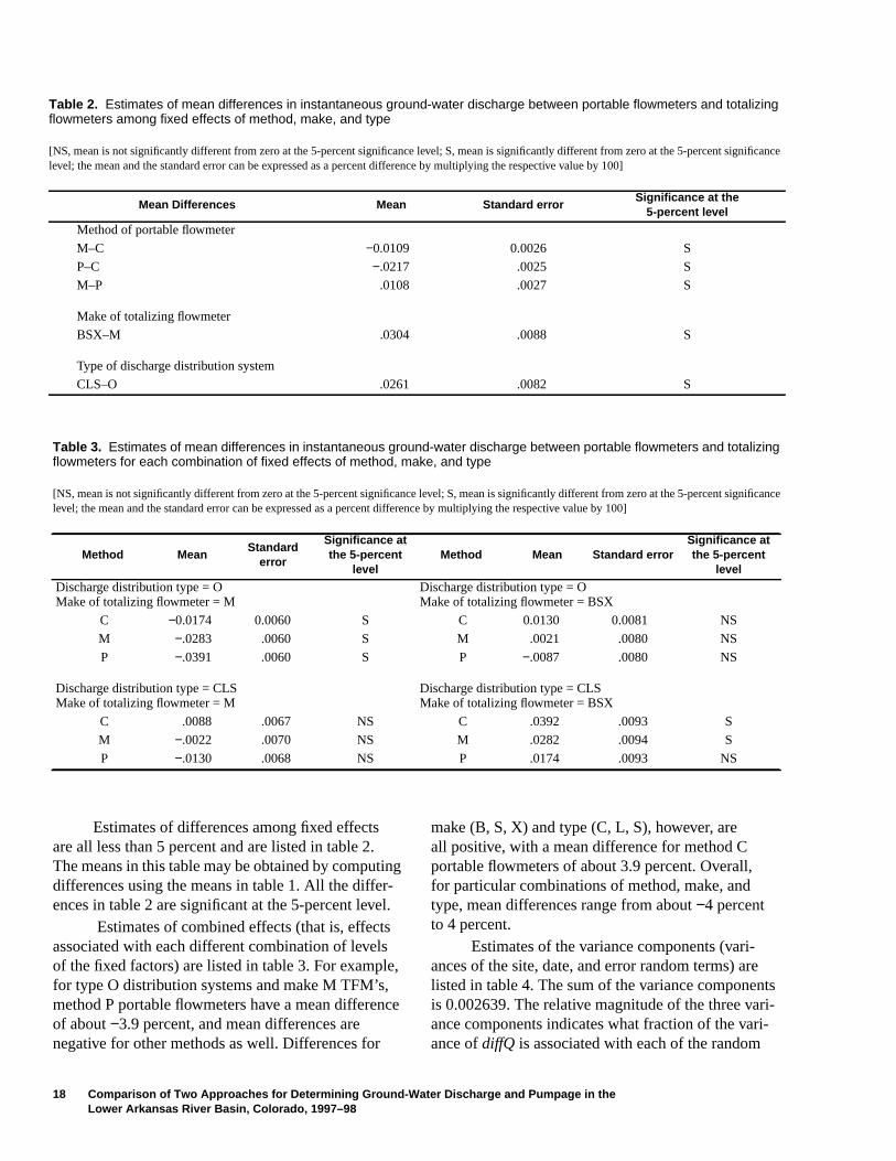
Table 2. Estimates of mean differences in instantaneous ground-water discharge between portable flowmeters and totalizingflowmeters among fixed effects of method, make, and type
[NS, mean is not significantly different from zero at the 5-percent significance level; S, mean is significantly different from zero at the 5-percent significancelevel; the mean and the standard error can be expressed as a percent difference by multiplying the respective value by 100]
Mean Differences Mean Standard errorSignificance at the
5-percent level
Method of portable flowmeter
M–C −0.0109 0.0026 S
P–C −.0217 .0025 S
M–P .0108 .0027 S
Make of totalizing flowmeter
BSX–M .0304 .0088 S
Type of discharge distribution system
CLS–O .0261 .0082 S
Table 3. Estimates of mean differences in instantaneous ground-water discharge between portable flowmeters and totalizingflowmeters for each combination of fixed effects of method, make, and type
[NS, mean is not significantly different from zero at the 5-percent significance level; S, mean is significantly different from zero at the 5-percent significancelevel; the mean and the standard error can be expressed as a percent difference by multiplying the respective value by 100]
Method MeanStandard
error
Significance atthe 5-percent
levelMethod Mean Standard error
Significance atthe 5-percent
level
Discharge distribution type = OMake of totalizing flowmeter = M
Discharge distribution type = OMake of totalizing flowmeter = BSX
C −0.0174 0.0060 S C 0.0130 0.0081 NS
M −.0283 .0060 S M .0021 .0080 NS
P −.0391 .0060 S P −.0087 .0080 NS
Discharge distribution type = CLSMake of totalizing flowmeter = M
Discharge distribution type = CLSMake of totalizing flowmeter = BSX
C .0088 .0067 NS C .0392 .0093 S
M −.0022 .0070 NS M .0282 .0094 S
P −.0130 .0068 NS P .0174 .0093 NS
Estimates of differences among fixed effectsare all less than 5 percent and are listed in table 2.The means in this table may be obtained by computingdifferences using the means in table 1. All the differ-ences in table 2 are significant at the 5-percent level.
Estimates of combined effects (that is, effectsassociated with each different combination of levelsof the fixed factors) are listed in table 3. For example,for type O distribution systems and make M TFM’s,method P portable flowmeters have a mean differenceof about−3.9 percent, and mean differences arenegative for other methods as well. Differences for
make (B, S, X) and type (C, L, S), however, areall positive, with a mean difference for method Cportable flowmeters of about 3.9 percent. Overall,for particular combinations of method, make, andtype, mean differences range from about−4 percentto 4 percent.
Estimates of the variance components (vari-ances of the site, date, and error random terms) arelisted in table 4. The sum of the variance componenis 0.002639. The relative magnitude of the three varance components indicates what fraction of the variance ofdiffQ is associated with each of the random
18 Comparison of Two Approaches for Determining Ground-Water Discharge and Pumpage in theLower Arkansas River Basin, Colorado, 1997–98

w-
or
te
-s
se
ny
e
’stnt
e-
terms in equation 5. Site-to-site variability accountsfor about 53 percent (100× 0.001399/ 0.002639) ofthe sum of the variance components, the date withinsite variability accounts for about 27 percent of thesum of the variance components, and the random errorterms accounts for the remaining 20 percent.
The total variance ofdiffQ around theoverall mean (that is, the variance ofdiffQ withouta model) is 0.003037, which indicates that thefixed effects account for about 13 percent [equals100× (0.003037− 0.002639) / 0.003037] of the vari-ance ofdiffQ. This is a relatively small part of the totalvariability, but the data set is large enough to result inthe statistically significant differences listed in tables 1through 3. Similarly, the site, date, and error variancecomponents expressed as a percent of the total vari-ance are 46 percent, 23 percent, and 18 percent,respectively. Overall, the largest portion of thevariance ofdiffQ is accounted for by site-to-sitevariability.
The random error variance (0.000539 in table 4)measures the amount of variability among differentportable flowmeter measurements applied on thesame day at the same site. The error variance can beused to determine the range in expected differencesbetween (logarithmically transformed) instantaneousdischarge measured using two different portable flow-meters. The estimated variance of the difference willbe 2× 0.000539 because the variance of the differencebetween two independent random variables is the sumof their variances. This translates into a standard devi-ation of about 3.28 percent. When this measure of therandom component of the difference is considered inconjunction with the systematic differences in table 2for different portable flowmeter methods, an estimateof the total error can be determined. For example, ifmeasurements are made using P and M portableflowmeters, the systematic bias (M–P) is 1.08 percentwith a standard deviation of 3.28 percent. If normality
is assumed, about 95 percent of the differencesbetween the measurements taken with the twoportable flowmeters will be between−5.48 percentand 7.64 percent.
The small size of the random error variancecomponent is indicated by the precision with whichdifferences among portable flowmeters can be esti-mated in table 2. The standard errors for portable flometer differences range from 0.25 to 0.27 percent,which is considerably smaller than standard errors fmake differences (0.88 percent) or type differences(0.82 percent). A strength of the design for this datacollection was the application of multiple portableflowmeter methods at the same well on the same daduring a short period of time.
TEMPORAL VARIATIONS IN POWERCONVERSION COEFFICIENTS
The use of PCC’s to estimate ground-waterpumpage from wells is most accurate when the relation of well discharge to power consumption remainstable. However, over time, hydrologic and pumpoperating conditions may change, thus altering thePCC relation to well discharge and power consump-tion. As examples, depth to ground water may increaafter an extended period of pumping or pump effi-ciency may decrease as the irrigation pump ages. Awell operation that results in significant variations inthe PCC over time can result in errors when using thPCC approach to estimate ground-water pumpage.
Short-Term Variations in PowerConversion Coefficients
Multiple PCC measurements repeated at thewell sites during 1997 and 1998 are used to indicatethe temporal variability in PCC’s during one and twoirrigation seasons. The range in PCC’s at 104 sitesduring 1998 is shown in figure 5A. The PCC’s for mostsites (86 percent) did not fluctuate more than20 percent throughout the 1998 irrigation season;however, for unknown reasons, a wide range in PCCoccurred at about 14 percent of the network sites. Asome wells, a lower than expected PCC measureme(site 5) or several lower than expected PCC measurments (site 27) resulted in the wide range in PCC’sthat were measured. The percent difference for the
Table 4. Estimates of the variances of the site, date, anderror random terms in discharge measurements
Random terms Variance
Site 0.001399
Date .000701
Error .000539
Sum 0.002639
TEMPORAL VARIATIONS IN POWER CONVERSION COEFFICIENTS 19

20 Comparison of Two Approaches for Determining Ground-Water Discharge and Pumpage in theLower Arkansas River Basin, Colorado, 1997–98
0
400
0
50
100
150
200
250
300
350
PO
WE
R C
ON
VE
RS
ION
CO
EF
FIC
IEN
T, I
N K
ILO
WA
TT
HO
UR
S P
ER
AC
RE
-FO
OT
0 1100 10 20 30 40 50 60 70 80 90 100
Minimum value
25th percentile
Median
75th percentile
Maximum value
0 1100 10 20 30 40 50 60 70 80 90 100
SITE
0
180
0
20
40
60
80
100
120
140
160
PE
RC
EN
T D
IFF
ER
EN
CE
LINE INDICATES 20-PERCENT DIFFERENCE
A
B
Note: Asterisk represents anindividual measurement
Figure 5. Power conversion coefficients (PCC) determined at network sites during 1998: (A) range in PCC and(B) percent difference.

es
7)
s
re-g
s
l
total range in PCC’s determined during 1998 is shownin figure 5B. The equation used to determine percentdifference shown in figure 5B is:
Percent difference = 100× (maximumPCC− minimum PCC)/site average PCC. (6)
Percent differences in PCC data at wells ranged fromless than 1 percent (sites 21 and 88) to more than150 percent (site 27). The data indicated that58 percent of the site comparisons had less than a10-percent change and 86 percent of the site compari-sons had less than a 20-percent change in PCC’sthroughout the 1998 irrigation season.
The PCC measurements made during the1998 irrigation season were evaluated for systematicseasonal variations. Figure 6 shows that for themajority of instances, there are no evident seasonalpatterns in the PCC measurements made during 1998.Comparisons of PCC’s to depth to ground water didnot reveal any systematic relation between changes inPCC’s and depth to water.
The PCC measurements made at 41 networksites during 1997 were compared to PCC measure-ments made during 1998 at the same 41 sites (fig. 7)to evaluate temporal variations during two irrigationseasons. Thirty-seven sites (90 percent) had at leastone PCC measurement made in 1997 that was lessthan the range of PCC’s made in 1998 (fig. 7); 16 ofthe sites (39 percent) had all 1997 PCC’s less than therange of PCC’s made during 1998. Only sites 83 and87 had a large difference between the 2 years of data.Overall, the 2 years of data indicate that the PCCmeasurements were similar between 1997 and 1998.
Long-Term Variations in PowerConversion Coefficients
State-approved PCC measurements collected atthe network sites during 1994 to 1997 for compliancewith State rules (Office of the State Engineer, 1994and 1996) were used to evaluate temporal variabilitythat occurred in PCC’s during the 4-year period. Thelong-term variability between PCC’s for wells in the1998 network and corresponding State-approvedPCC’s during 1994–97 is shown in figure 8A. Implicitin this comparison is the assumption that the State-approved PCC’s determined during 1994–97 are of thesame quality as the PCC’s determined during this
study, including the removal of the cases where thePCC’s change under Rule 3.5 (Office of the StateEngineer, 1996) due to a change in pump or motor.The equation used to compute the percent differencshown in figure 8B is:
Percent difference = 100× (State-approvedPCC− site average PCC)/site average PCC, (
wheresite average PCC = the arithmetic mean of all PCC’
determined at each site in 1998.Fifty comparisons of 103 PCC measure-
ments (about 48 percent) had less than 10-percentdifference between the State-approved PCC’s andthe site average PCC measured during 1998 andabout 67 percent of the State-approved PCC measuments were less than 20 percent of the PCC’s durin1998 (table 5). Twenty-one of the 103 site compari-sons indicated a positive percent difference of morethan 20 percent in PCC’s, and 13 site comparisonsindicated a negative percent difference of more than20 percent. A positive percent difference indicatedthat the 1994–97 State-approved PCC was greaterthan the site average PCC in 1998.
The percent difference between the State-approved 1994–97 PCC’s and the average 1998PCC ranged from about−57 to 211 (table 5). Thelargest range in percent difference was between theState-approved PCC’s measured in 1995 and the1998 PCC’s. A comparison of the percent differencecomputed using the State-approved PCC’s from1997 to the average 1998 PCC’s indicated that78 percent of the sites were within 10 percent and89 percent of the sites were within 20 percent.
During well operation, the PCC is generallyconstant for a specific discharge pressure and astable pumping water level. Because the water levein a well often declines rapidly during the initialperiod of pumping, the PCC also changes rapidlyuntil the pumping water level stabilizes. A potentiallyimportant change made in the Colorado amendedrules in 1996 (Office of the State Engineer, 1996)required PCC measurements be made only after thepumping water level had not changed more than10 percent in the hour prior to making the PCCmeasurement.
TEMPORAL VARIATIONS IN POWER CONVERSION COEFFICIENTS 21
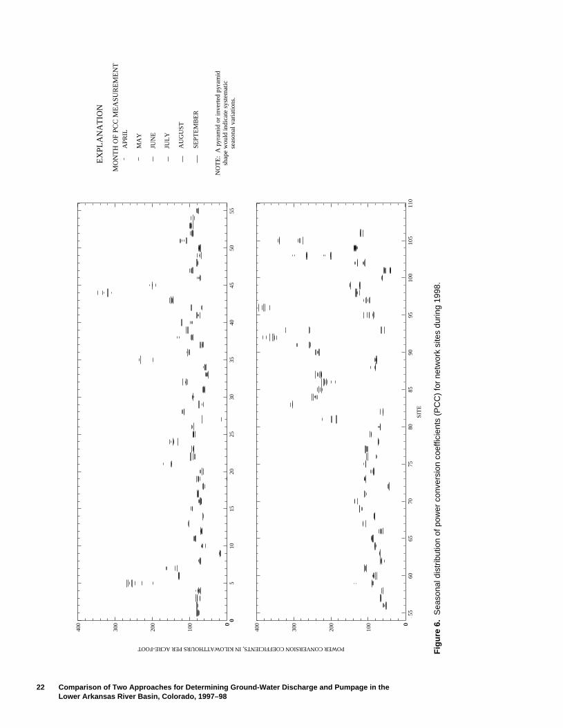
22 Comparison of Two Approaches for Determining Ground-Water Discharge and Pumpage in theLower Arkansas River Basin, Colorado, 1997–98
056
05
1015
2025
3035
4045
5055
0
400 0
100
200
300
AP
RIL
MA
Y
JUN
E
JULY
AU
GU
ST
SE
PT
EM
BE
R
EX
PLA
NA
TIO
N
NO
TE
: A
pyr
amid
or
inve
rted
pyr
amid
sha
pe w
ould
indi
cate
sys
tem
atic
seas
onal
var
iatio
ns.
5411
055
6065
7075
8085
9095
100
105
SIT
E
0
400 0
100
200
300
POWER CONVERSION COEFFICIENTS, IN KILOWATTHOURS PER ACRE-FOOT
MO
NT
H O
F P
CC
ME
AS
UR
EM
EN
T
Fig
ure
6. S
easo
nal d
istr
ibut
ion
of p
ower
con
vers
ion
coef
ficie
nts
(PC
C)
for
netw
ork
site
s du
ring
1998
.

TE
MP
OR
AL V
AR
IAT
ION
S IN
PO
WE
R C
ON
VE
RS
ION
CO
EF
FIC
IEN
TS
23
0 1100 10 20 30 40 50 60 70 80 90 100
SITE
40
400
40
60
80
100
120
140
160
180
200
220
240
260
280
300
320
340
360
380
PO
WE
R C
ON
VE
RS
ION
CO
EF
FIC
IEN
T, I
N K
ILO
WA
TT
SH
OU
RS
PE
R A
CR
E-F
OO
T
Minimum value
25th percentile
Median
75th percentile
Maximum value
1998 Data
1997 Data
Figure 7. Power conversion coefficients (PCC) determined at selected network sites during 1997 and 1998.
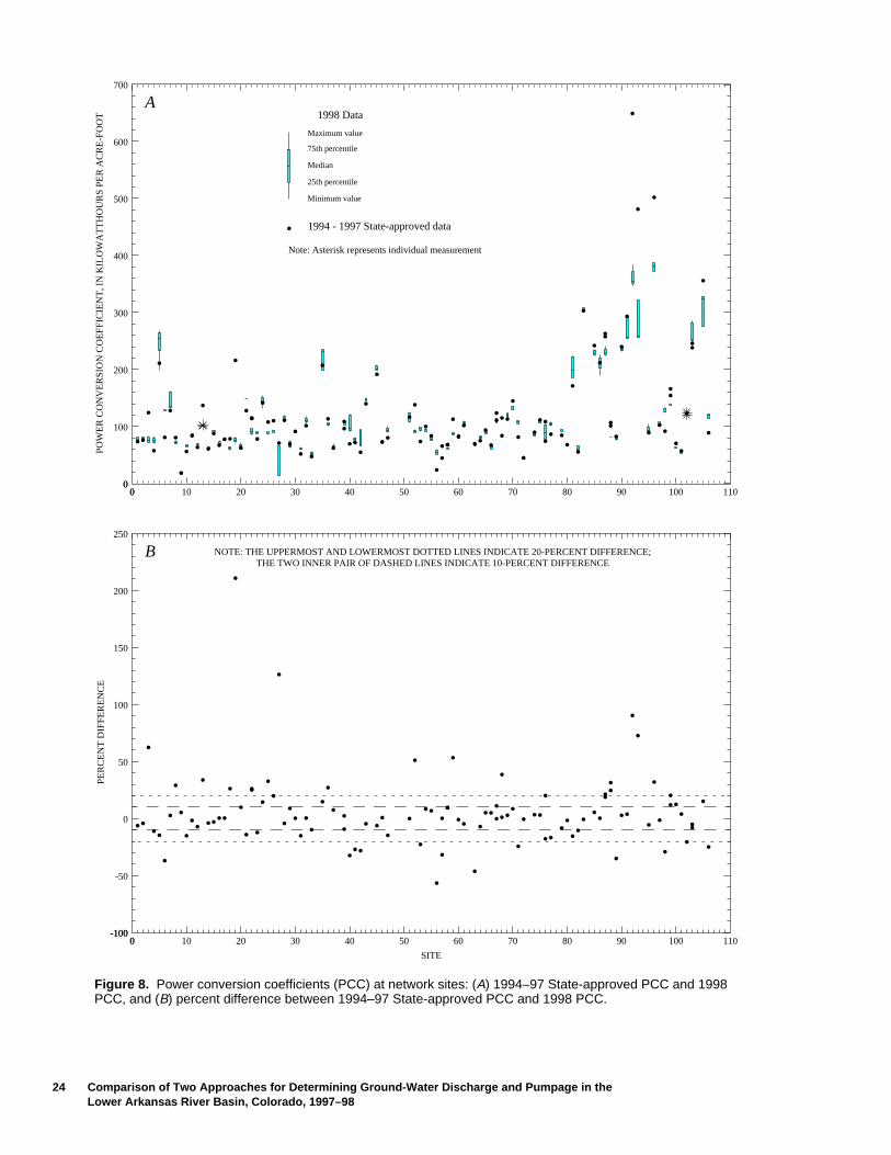
24 Comparison of Two Approaches for Determining Ground-Water Discharge and Pumpage in theLower Arkansas River Basin, Colorado, 1997–98
0
700
0
100
200
300
400
500
600
PO
WE
R C
ON
VE
RS
ION
CO
EF
FIC
IEN
T, I
N K
ILO
WA
TT
HO
UR
S P
ER
AC
RE
-FO
OT
0 1100 10 20 30 40 50 60 70 80 90 100
Minimum value
25th percentile
Median
75th percentile
Maximum value
1998 Data
1994 - 1997 State-approved data
0 1100 10 20 30 40 50 60 70 80 90 100
SITE
-100
250
-100
-50
0
50
100
150
200
PE
RC
EN
T D
IFF
ER
EN
CE
NOTE: THE UPPERMOST AND LOWERMOST DOTTED LINES INDICATE 20-PERCENT DIFFERENCE;THE TWO INNER PAIR OF DASHED LINES INDICATE 10-PERCENT DIFFERENCE
A
B
Note: Asterisk represents individual measurement
Figure 8. Power conversion coefficients (PCC) at network sites: (A) 1994–97 State-approved PCC and 1998PCC, and (B) percent difference between 1994–97 State-approved PCC and 1998 PCC.

sells
n
anoase
d
alt
at
Table 5. Comparison of State-approved power conversion coefficient (PCC) measurements (1994–97) to the site averagePCC measurements made during 1998
[PCC, power conversion coefficient]
State-approved PCCmeasurement year
Number of PCCcomparisons
Minimum andmaximum percent
difference
Number of PCCcomparisons within
10 percent of 1998 siteaverage PCC
Number of PCCcomparisons within
20 percent of 1998 siteaverage PCC
Number Percent Number Percent
1994 37 −5790
18 49 25 68
1995 26 −37211
8 31 11 42
1996 22 −4627
10 45 17 77
1997 18 −1873
14 78 16 89
1994–97 103 −57211
50 48 69 67
COMPARISON OF GROUND-WATERPUMPAGE ESTIMATES
A comparison of ground-water pumpagemeasured using TFM’s to ground-water pumpage esti-mates determined by the PCC approach was made byevaluating the differences in pumpage and deter-mining whether the differences are statistically signifi-cant. The pumpage estimates were calculated usingPCC measurements made at network sites during1998. This was done by dividing the total 1998 powerconsumed at each site during the monitoring period, inkilowatthours, by each unique PCC measurementmade at that same well site during 1998. The TFMderived pumpage measurement at each well was deter-mined as the difference between TFM readings madeat the beginning and the end of the monitoring period.The monitoring period was the same for the TFM andPCC approach. Because it was determined that themethod of portable flowmeter, make of TFM,discharge distribution type, and the site, date, andrandom error were identified as sources of variation,an additional level of data analysis was required.
This section of the report presents (1) themagnitude in differences in ground-water pumpagebetween TFM and PCC estimates; (2) an estimate ofthe overall mean difference in pumpage and whetherthe overall mean difference is significantly differentfrom zero; (3) an estimate of the mean differences foreach combination of portable flow meter, make ofTFM, and discharge distribution type, and whether
these mean differences are significantly different fromzero. The comparison of ground-water pumpage wabased on 553 paired measurements made at 103 wduring 1998.
Primary Results
The analysis of variance on the differences inpumpage was performed using a rank transformatioon 553 paired pumpage measurements made at103 wells during 1998. About 80 percent of thedifferences in pumpage between the TFM and PCCapproach were less than 10 percent. The overall medifference in pumpage was 0.01 percent, indicating nsignificant difference on average between pumpagemeasured by TFM and pumpage as computed by thPCC approach. For varying site characteristics (themethod of portable flowmeter, the make of TFM, antype of discharge distribution system), mean differ-ences in pumpage were generally less than±3 percentand, for most instances, the mean differences in totpumpage were not significantly different from zero athe 5-percent level.
Details of Analysis and Results
For each paired pumpage measurement madea well, the difference in ground-water pumpage,diffP,was computed as:
COMPARISON OF GROUND-WATER PUMPAGE ESTIMATES 25

nt,
ns
ors
tede
r
ei-
t;
.
, (8)
where denotes estimated pumpage as calculated bythe PCC approach, andV denotes a correspondingtotal pumpage as measured by a TFM. As with instan-taneous discharge measurements, a log transformationwas used, so that the variable of interest is the differ-ence between the log-transformed values.
BecausediffP is a random variable likediffQ,the probability distribution must be characterized.However, as mentioned earlier in the report, unlikediffQ, the distribution fordiffP deviated significantlyfrom normality. There are a number of data valuesfound outside the range of the majority of data values,and such a deviation from normality can cause seriousproblems with analysis of variance. Therefore, a ranktransformation was performed on the data beforeperforming the analysis, and an inverse rank transfor-mation (linear approximation) to the results of theanalysis of variance provided estimates of the centraltendency of the distribution ofdiffP. Use of the ranktransformation in analysis of variance is discussed byIman and Conover (1981), Helsel and Hirsch (1992),Kepner and Wackerly (1996) and Hora and Iman(1988). Rank transformation does not render thetest truly nonparametric, but asymptotic normal theoryshould be more applicable than would be the case ifusing untransformed data. Rank transformation mini-mizes the influence of very large outliers so that theanalysis better reflects the central tendency of thedata. Evaluating the data without the influence ofextreme outliers was essential in understanding thedata, and the results of this analysis indicated the typesof errors in estimation of pumpage expected at atypical site under typical circumstances. Because atypical-site analysis is inadequate when analyzingaggregated pumpage for a number of wells, a separateanalysis of this problem is discussed later in the reportin the section titled “Estimation of Total NetworkPumpage”.
The overall pattern of differences betweenV and are illustrated in figure 9A, which is a plot ofdiffP
versusV, and in figure 9B, which is a plot of the differ-ence in untransformed pumpage versusV. These plotsare analogous to the plots in figure 2A and 2B fordischarge. Variability about the mean tends to be morenearly constant in figure 9A than in figure 9B for mostof the data, so making a logarithmic transformation onthe variables is reasonable. These plots also show
clearly that there is a small proportion of the differ-ences for whichdiffP tends to be outside the rangeof the majority of the data.
Boxplots ofdiffP for all the data pooled and foreach level of method, make, and type are shown infigure 10. About 80 percent of the differences inpumpage estimates between the TFM and PCCapproach were less than 10 percent, more than50 percent of the differences were less than 6 perceand the median difference was about 1 percent(fig. 10A). The distribution of the differences variedsomewhat depending on method, make, and type(figs. 10B, 10C, and 10D).
The analysis of variance model was firstapplied using all levels of each of the fixed factors:method, make, and type. Significant differencesoccurred between all pairs of methods, but notbetween different makes or types. However,pooling the pumpage data in the same manneras the discharge data allows direct comparisonsbetween results of the two analyses. Such comparisoare useful and can be used to determine how errorsin instantaneous discharge measurements affect errin pumpage calculations. Thus, the analysis wasredone using the same pooling described in the“Comparison of Instantaneous Ground-WaterDischarge Measurements” section. Diagnosticplots again indicated satisfactory adherence tothe analysis of variance assumptions.
Final results of the analysis of variance arelisted in tables 6 through 8 and are analogous to theresults for the instantaneous discharge data presenin tables 1 through 3. As stated earlier, results from thanalysis of variance is in terms of ranks, so a linearapproximation to the rank-transformation curve neathe median was used to back-transform and obtainresults in terms ofdiffP. Differences in estimates of themean differences listed in tables 6 through 8 that armore than 2 standard errors from zero again are indcated as being statistically significant.
The overall grand mean difference for allpossible pairs of pumpage in table 6 is 0.0001(0.01 percent), again almost zero. The estimatesfor the portable flowmeter method effects were: formethod C, 0.73 percent; for method M, 0.22 percenand for method P,−0.93 percent. These effects arecomparable in magnitude to portable flowmetermethod effects for the well discharge data in table 1Similarly, signs of the make and type effects are the
diffP V( ) V( )log–log=
V
V
26 Comparison of Two Approaches for Determining Ground-Water Discharge and Pumpage in theLower Arkansas River Basin, Colorado, 1997–98

COMPARISON OF GROUND-WATER PUMPAGE ESTIMATES 27
0.05 1,0000.1 0.2 0.5 1 2 5 10 20 50 100 200 500-0.5
2.5
-0.5
0
0.5
1.0
1.5
2.0
DIF
FE
RE
NC
ES
IN G
RO
UN
D-W
AT
ER
PU
MP
AG
E, I
N L
OG
AR
ITH
MIC
UN
ITS
0.05 1,0000.1 0.2 0.5 1 2 5 10 20 50 100 200 500
TOTALIZING FLOWMETER PUMPAGE, IN ACRE-FEET
-200
60
-200
-180
-160
-140
-120
-100
-80
-60
-40
-20
0
20
40
DIF
FE
RE
NC
ES
IN G
RO
UN
D-W
AT
ER
PU
MP
AG
E, I
N A
CR
E-F
EE
T
A
B
Figure 9. Relation of ground-water pumpage from inline totalizing flowmeter to the differences in pumpage esti-mates between power conversion coefficient approach and totalizing flowmeters, expressed (A) in logarithmicunits and (B) in acre-feet.

28 Comparison of Two Approaches for Determining Ground-Water Discharge and Pumpage in theLower Arkansas River Basin, Colorado, 1997–98
(553)
-0.3
0.3
-0.3
-0.2
-0.1
0
0.1
0.2
0.3
DIF
FE
RE
NC
ES
IN G
RO
UN
D-W
AT
ER
PU
MP
AG
E, I
N L
OG
AR
ITH
MIC
UN
ITS
EXPLANATION
10th percentile
25th percentile
Median
75th percentile
90th percentile
10th and 90th percentilesData values outside the
(553) Number of observations
(236) (150)(167)
P C M
PORTABLE FLOWMETER METHOD
-0.3
0.3
-0.3
-0.2
-0.1
0
0.1
0.2
0.3
(53)(81)(358) (61)
O L S C
TYPE OF DISCHARGE DISTRIBUTION SYSTEM
-0.3
0.3
-0.3
-0.2
-0.1
0
0.1
0.2
0.3
Note: Twenty-one outliers are not shown
ENTIRENETWORK
90 percentile = 0.85is not shown
(25)(395) (114) (19)
M S X B
MAKE OF TOTALIZING FLOWMETER
-0.3
0.3
-0.3
-0.2
-0.1
0
0.1
0.2
0.3
DIF
FE
RE
NC
ES
IN G
RO
UN
D-W
AT
ER
PU
MP
AG
E, I
N L
OG
AR
ITH
MIC
UN
ITS
A B
C D
PORTABLE FLOWMETER METHOD:P= Polysonic; C= Collins; M= McCrometer
MAKE OF TOTALIZING FLOWMETER:M=McCrometer, S= Signet;
X= preexisting McCrometer; B= Badger
TYPE OF DISCHARGE DISTRIBUTION SYSTEM:O= open; L= low pressure; S= sprinkler
C= complex
Figure 10. Boxplots showing differences in ground-water pumpage estimates between power conversion coefficientapproach and totalizing flowmeters (A) for the entire network, (B) by portable flowmeter method, (C) by make of totalizingflowmeter, and (D) by type of discharge distribution system, 1998.

-sis
same as for the discharge analysis, but the magnitudeof the effects for pumpage estimates is somewhatsmaller. Most of the differences shown in table 6 arenot statistically significant.
In table 7, estimates of mean differences amongthe three fixed effects are less than±2.04 percent. Thesmall standard errors for these differences reflect theincrease in precision due to use of more than oneportable flowmeter method at the same well on thesame day.
The largest positive value for the combinedeffects (table 8) is 2.44 percent for type (CLS),make (BSX), and method C. The most negative value
in table 8 is−2.63 percent for type O, make M, andmethod P. Both of these extreme values are statisti-cally significant, but most other combined effects intable 8 are not.
A linear approximation for the back-transformation from ranks provided good resultsfor the estimated mean values in tables 6 through 8because these values were all near zero. However,such a linearization technique applied to variancesis questionable because of increasing effects of nonlinearity for errors far from zero. Therefore, estimateof the variance components for the pumpage analysare not presented.
COMPARISON OF GROUND-WATER PUMPAGE ESTIMATES 29
Table 6. Estimates of mean differences in pumpage between power conversion coefficient approach and totalizing flowmeterfor the grand mean and fixed effects of method, make, and type
[NS, mean is not significantly different from zero at the 5-percent significance level; S, mean is significantly different from zero at the 5-percent significancelevel; the mean and the standard error can be expressed as a percent difference by multiplying the respective value by 100
Mean differences Mean Standard errorSignificance at the
5-percent level
Grand mean 0.0001 0.0046 NSMethod of portable flowmeter (fixed)
C .0073 .0047 NSM .0022 .0048 NSP −.0093 .0047 NS
Make of totalizing flowmeter (fixed)
M −.0101 .0048 SBSX .0103 .0077 NS
Type of discharge distribution system (fixed)
O −.0068 .0053 NSCLS .0070 .0069 NS
Table 7. Estimates of mean differences in pumpage between power conversion coefficient approach and totalizing flowmeteramong fixed effects of method, make, and type
[NS, mean is not significantly different from zero at the 5-percent significance level; S, mean is significantly different from zero at the 5-percent significancelevel; the mean and the standard error can be expressed as a percent difference by multiplying the respective value by 100]
Mean differences Mean Standard errorSignificance at the
5-percent level
Method of portable flowmeterM–C −0.0052 0.0021 SP–C −.0166 .0020 SM–P .0114 .0023 S
Make of totalizing flowmeterBSX–M .0204 .0089 S
Type of discharge distribution systemCLS–O .0138 .0082 NS

s
le
-
ered
r
he
ofalne
s
ee-
Table 8. Estimates of mean differences in pumpage between power conversion coefficient approach and totalizing flowmeterfor each combination of fixed effects of method, make, and type
[NS, mean is not significantly different from zero at the 5-percent significance level; S, mean is significantly different from zero at the 5-percent significancelevel; the mean and the standard error can be expressed as a percent difference by multiplying the respective value by 100]
Method MeanStandard
error
Significance atthe 5-percent
levelMethod Mean
Standarderror
Significance atthe 5-percent
level
Discharge distribution type = OMake of totalizing flowmeter = M
Discharge distribution type = OMake of totalizing flowmeter = BSX
C −0.0097 0.0058 NS C 0.0106 0.0080 NS M −.0149 .0059 S M .0055 .0080 NS P −.0263 .0059 S P −.0060 .0080 NS
Discharge distribution type = CLSMake of totalizing flowmeter = M
Discharge distribution type = CLSMake of totalizing flowmeter = BSX
C .0040 .0068 NS C .0244 .0094 S M −.0011 .0070 NS M .0192 .0096 NS P −.0126 .0069 NS P .0078 .0095 NS
SOURCES OF DISCREPANCY BETWEENPUMPAGE ESTIMATES
The analysis of variance procedures applied toinstantaneous discharge and pumpage data providedinformation on the mean differences in well discharge(diffQ) and pumpage (diffP) and on the variance ofdiffQ. It is clear, however, that these analyses are notindependent of each other. Part of the discrepancybetween total pumpage computed by the PCCapproach and pumpage measured by the TFM comesfrom differences between measurements made byportable flowmeters and TFM’s and differencesbetween these meters are reflected in differencesbetween the paired instantaneous discharge measure-ments. In other words, one would expect that part ofthe variability indiffP is being caused by variability indiffQ. However, there are other possible sources ofdiscrepancy between total pumpage obtained by thetwo approaches. The following section of the reportenumerates several possible sources of discrepancy.For most of these sources, data are not available toestimate exactly how much of the discrepancy iscoming from each source. Nevertheless, it is importantto explicitly discuss what the possible sources of errorare, possibly providing guidance for future data-collection efforts. One important source of potentialdiscrepancy that is discussed in some detail istemporal variability of the PCC. Some data are avail-able to obtain an estimate of the contribution of thiscomponent to the difference between pumpage by thetwo approaches.
Specifically, this section of the report discusse(1) possible sources of discrepancy that result indifferences between ground-water pumpage asmeasured by a TFM and ground-water pumpage asobtained by the PCC approach; and (2) with availabdata, how might the temporal variability of PCC’seffect the differences in pumpage.
Primary Results
There are several potential sources of discrepancy between pumpage as measured by a TFM andpumpage as computed by the PCC approach. Thesinclude errors in instantaneous discharge as measuby a TFM and a portable flowmeter, TFM pumpageerrors, errors in the electrical power meter, andtemporal variability of the PCC. Each may account foa portion of the discrepancy between pumpage asmeasured by a TFM and pumpage as computed by tPCC approach. It is not possible with data currentlyavailable to give reliable estimates of the magnitudeeach of the components of pumpage error. Additiondata and evaluation of these data are needed to defilong-term temporal variations in PCC’s and TFM’s, awell as defining other sources of discrepancy inpumpage estimates.
Limited data are available to provide an estimatof errors caused by temporal variability of PCC’s. Thstandard deviation associated with year-to-year variability of these PCC’s was estimated to be about
30 Comparison of Two Approaches for Determining Ground-Water Discharge and Pumpage in theLower Arkansas River Basin, Colorado, 1997–98
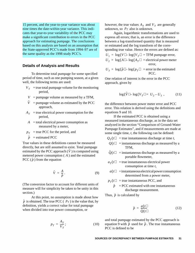
d
s:
d
etr
e at
a
a
n
iss
15 percent, and the year-to-year variance was aboutnine times the date-within-year variance. This indi-cates that year-to-year variability of the PCC maymake a significant contribution to errors in the PCCapproach for estimating pumpage. The conclusionsbased on this analysis are based on an assumption thatthe State-approved PCC’s made from 1994–97 are ofthe same quality as the 1998 study PCC’s.
Details of Analysis and Results
To determine total pumpage for some specifiedperiod of time, such as one pumping season, at a givenwell, the following terms are used:
= true total pumpage volume for the monitoringperiod,
= pumpage volume as measured by a TFM,
= pumpage volume as estimated by the PCCapproach,
= true electrical power consumption for theperiod,
= total electrical power consumption asmeasured by a meter,
= true PCC for the period, and
= estimated PCC
True values in these definitions cannot be measureddirectly, but are still assumed to exist. Total pumpageestimated by the PCC approach ( ) is computed usingmetered power consumption ( ) and the estimatedPCC ( ) from the equation
. (9)
(The conversion factor to account for different units ofmeasure will for simplicity be taken to be unity in thissection.)
At this point, no assumption is made about howis obtained. The true PCC ( ) is the value that, by
definition, yields a correct value for total pumpagewhen divided into true power consumption, or
; (10)
however, the true values and are generallyunknown, so also is unknown.
Again, logarithmic transformations are used toexpress all errors; that is, an error is the differencebetween a log-transformed quantity that is measureor estimated and the log transform of the corre-sponding true value. Hence the errors are defined a
= TFM pumpage error,
= electrical power metererror,
= error in the estimatedPCC.
One relation of interest is the error in the PCCapproach, given by
, (11)
the difference between power meter error and PCCerror. This relation is derived using the definitions anequations 9 and 10.
If the estimated PCC is obtained using ameasured instantaneous discharge, as in the data sanalyzed in the section “Comparison of Ground-WatePumpage Estimates”, and if measurements are madsome single time,t, the following can be defined:
= true instantaneous discharge at timet,
= instantaneous discharge as measured byTFM,
= instantaneous discharge as measured byportable flowmeter,
= true instantaneous electrical powerconsumption at timet,
=instantaneouselectricalpowerconsumptiodetermined from a power meter,
= true instantaneous PCC, and
= PCC estimated with one instantaneousdischarge measurement.
Thus, is calculated by
(12)
and total pumpage estimated by the PCC approachequation 9 with used for . The true instantaneouPCC is defined to be
VT
V
V
AT
A
pT
p
VA
p
VAp---=
p pT
pT
AT
VT-------=
AT VTpT
U1 V( ) VT( )log–log=
U2 A( ) AT( )log–log=
U3 p( ) pT( )log–log=
V( ) VT( )log–log U2 U3–=
QT t( )Q t( )
Q t( )
aT t( )
a t( )
pT t( )p
p
pa t( )Q t( )-----------=
p p
SOURCES OF DISCREPANCY BETWEEN PUMPAGE ESTIMATES 31
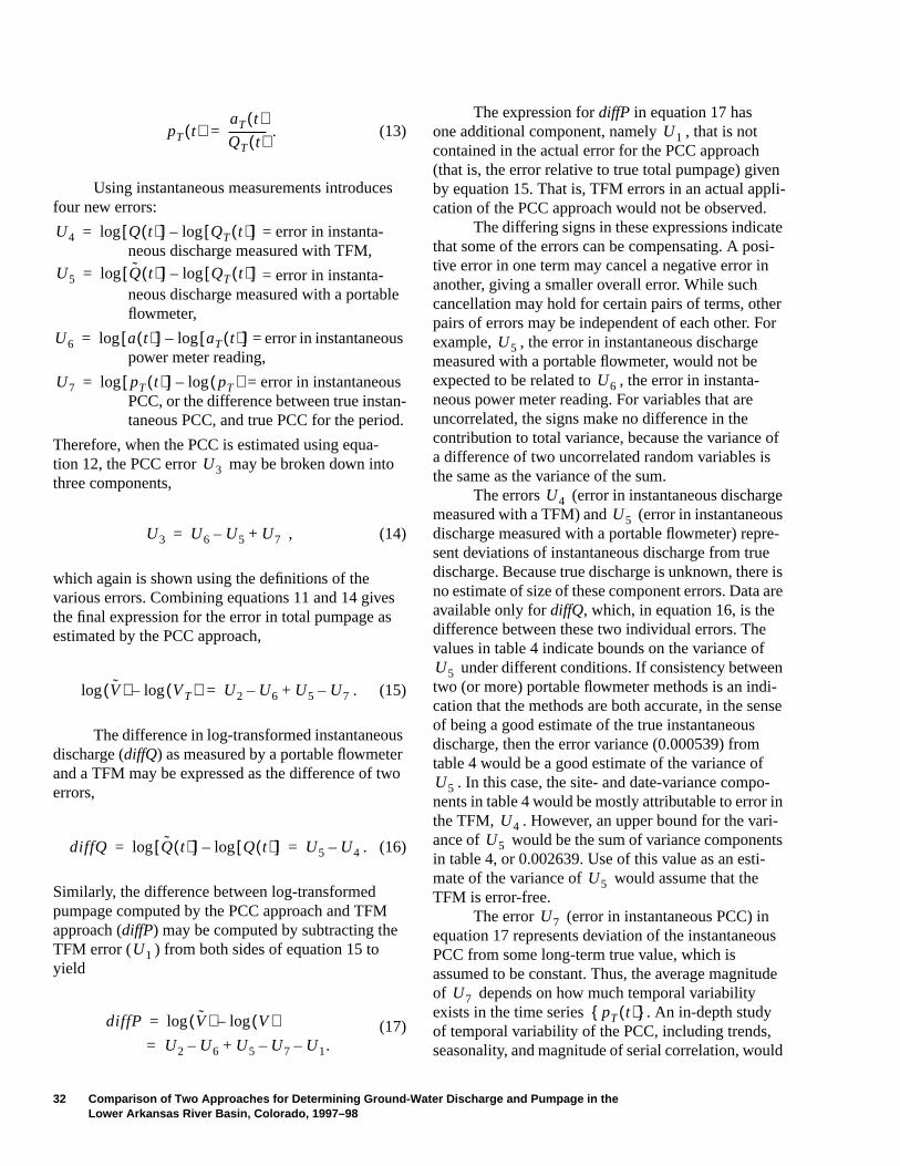
nli-
ei-
ror
of
ese-
isre
n-nse
-n-ts
us
de
ld
. (13)
Using instantaneous measurements introducesfour new errors:
= error in instanta-neous discharge measured with TFM,
= error in instanta-neous discharge measured with a portableflowmeter,
= error in instantaneouspower meter reading,
= error in instantaneousPCC, or the difference between true instan-taneous PCC, and true PCC for the period.
Therefore, when the PCC is estimated using equa-tion 12, the PCC error may be broken down intothree components,
, (14)
which again is shown using the definitions of thevarious errors. Combining equations 11 and 14 givesthe final expression for the error in total pumpage asestimated by the PCC approach,
. (15)
The difference in log-transformed instantaneousdischarge (diffQ) as measured by a portable flowmeterand a TFM may be expressed as the difference of twoerrors,
. (16)
Similarly, the difference between log-transformedpumpage computed by the PCC approach and TFMapproach (diffP) may be computed by subtracting theTFM error ( ) from both sides of equation 15 toyield
(17)
The expression fordiffP in equation 17 hasone additional component, namely , that is notcontained in the actual error for the PCC approach(that is, the error relative to true total pumpage) giveby equation 15. That is, TFM errors in an actual appcation of the PCC approach would not be observed.
The differing signs in these expressions indicatthat some of the errors can be compensating. A postive error in one term may cancel a negative error inanother, giving a smaller overall error. While suchcancellation may hold for certain pairs of terms, othepairs of errors may be independent of each other. Fexample, , the error in instantaneous dischargemeasured with a portable flowmeter, would not beexpected to be related to , the error in instanta-neous power meter reading. For variables that areuncorrelated, the signs make no difference in thecontribution to total variance, because the variance a difference of two uncorrelated random variables isthe same as the variance of the sum.
The errors (error in instantaneous dischargmeasured with a TFM) and (error in instantaneoudischarge measured with a portable flowmeter) reprsent deviations of instantaneous discharge from truedischarge. Because true discharge is unknown, thereno estimate of size of these component errors. Data aavailable only fordiffQ, which, in equation 16, is thedifference between these two individual errors. Thevalues in table 4 indicate bounds on the variance of
under different conditions. If consistency betweetwo (or more) portable flowmeter methods is an indication that the methods are both accurate, in the seof being a good estimate of the true instantaneousdischarge, then the error variance (0.000539) fromtable 4 would be a good estimate of the variance of
. In this case, the site- and date-variance components in table 4 would be mostly attributable to error ithe TFM, . However, an upper bound for the variance of would be the sum of variance componenin table 4, or 0.002639. Use of this value as an esti-mate of the variance of would assume that theTFM is error-free.
The error (error in instantaneous PCC) inequation 17 represents deviation of the instantaneoPCC from some long-term true value, which isassumed to be constant. Thus, the average magnituof depends on how much temporal variabilityexists in the time series . An in-depth studyof temporal variability of the PCC, including trends,seasonality, and magnitude of serial correlation, wou
pT t( )aT t( )QT t( )--------------=
U4 Q t( )[ ] QT t( )[ ]log–log=
U5 Q t( )[ ] QT t( )[ ]log–log=
U6 a t( )[ ] aT t( )[ ]log–log=
U7 pT t( )[ ] pT( )log–log=
U3
U3 U6 U5– U7+=
V( ) VT( )log–log U2 U6– U5 U7–+=
diffQ Q t( )[ ] Q t( )[ ]log–log U5 U4–= =
U1
diffP V( ) V( )log–log=
= U2 U6– U5 U7– U1.–+
U1
U5
U6
U4U5
U5
U5
U4U5
U5
U7
U7pT t( ){ }
32 Comparison of Two Approaches for Determining Ground-Water Discharge and Pumpage in theLower Arkansas River Basin, Colorado, 1997–98

nd
-y
t
anf
th
e
rd
a.
via-
need detailed data on , which are not availablefor any of the sites. Therefore, a simpler approach wasused to obtain an idea of the short- and long-term vari-abilities in PCC. This approach uses the State-approved PCC’s made from 1994–97 together with thePCC’s made in 1998 as part of this study. One poten-tial fallacy in this approach is the implicit assumptionthat the quality of the State-approved PCC’s madefrom 1994–97 is the same as the quality of the PCC’smade during this study. If this assumption is accepted,then the temporal variability in PCC can be evaluated.If the PCC data are not of the same quality, then errorsnot associated with temporal variability could beattributed to the errors in temporal variability in thefollowing analyses, resulting in an inflated estimate ofthe year-to-year variability.
A nested variance-components analysis usingrandom terms for site, year within site, and datewithin year and site, was performed using all the log-transformed PCC values, including the 1998 valuesand 106 State-approved PCC’s from 1994–97. Onceagain, fixed effects (method, make, and type) were notincluded in the analysis. Such a nested model that hasterms representing variability at different time scales isone way of modeling temporal correlation. The esti-mate of the variance for the year component was0.02297, for the date-within-year component was0.00254, and for the residual variance was 0.00077.The year component represents about a 15-percentstandard deviation (obtained by taking the square rootof the variance and multiplying by 100). This indicatesthat the year-to-year variability could be a majorcomponent of variability for this PCC data set; theyear variance component is about nine times the vari-ance of date-within-year component. The PCC valuesused in this analysis contained uncertainty due toerrors in instantaneous discharge as measured by theportable flowmeter as well as errors in instantaneouspower meter reading (see eq. 14). This means that anestimate of the variance of (error in instantaneousPCC) using this analysis is inflated somewhat. Basedon the estimates given in the preceding paragraph,however, errors in discharge as measured by a portableflowmeter would not account for much of the year-to-year variability in the PCC (fig. 8B). To accuratelyquantify the temporal variability in the PCC, long-term time series PCC data are needed.
Errors (TFM pumpage error) and(electrical power meter error) represent errors in thelong-term integrated values of discharge and power
consumption, respectively. The first error (U1)would result from a TFM that is malfunctioning andproviding consistently biased readings, and the secoerror (U2) would result from a malfunctioning elec-trical meter. Although no data are available for evaluating the magnitude of these errors, one or both mabe at least partly responsible for the extreme differ-ences in pumpage (diffP) seen in figure 9A. Compo-nent (TFM pumpage error) would not be presenwhen comparing PCC-estimated pumpage to truepumpage (eq. 15). Finally, errors and , inte-grated and instantaneous power meter error, maysomewhat compensate for each other if the errorsresult from a malfunctioning power meter.
ESTIMATION OF TOTAL NETWORKPUMPAGE
The analysis presented earlier in the report,in the “Comparison of Ground-Water PumpageEstimates” section, provided estimates of the meanor average differences between the log-transformedPCC-estimated total pumpage and TFM-measuredtotal pumpage,diffP, at a well. However, it also isimportant to quantify the differences in the total oraggregated pumpage for a network of wells.
Primary Results
An analysis of the pumpage data was done todetermine differences in the total or aggregatedpumpage between the TFM and PCC approach for network of wells. The difference in pumpage betweethe TFM and PCC approach varied with the volume owater pumped during the 1998 monitoring period.Some wells that recorded small pumpage exhibitedlarger percent differences than wells with largerpumpage. Because of these unequal differences wirespect to total pumpage, it was necessary to groupor stratify the data based on the magnitude of totalpumpage for the 1998 monitoring period. Because thcorrect number of groupings, or strata, is not knownwith the information available, the mean and standadeviation of differences in the total pumpage wasdetermined conditionally for several numbers of stratFor a network of 103 wells and a number of stratagreater than 10, the resulting mean and standard detion leads to a conclusion that, for any given year,
pT t( ){ }
U7
U1 U2
U1
U2 U6
ESTIMATION OF TOTAL NETWORK PUMPAGE 33

ct
l
of
ee
fi--
-a
fat
a.
oci-a
-
there is a 95-percent probability that the differencein aggregated pumpage between the TFM and PCCapproach would be between about−3.41 and1.59 percent. The analysis indicates that the differencein aggregated pumpage would be expected to besmaller as the number of wells becomes larger.Assuming the distribution of total TFM pumpage isthe same for 1998 data set, there is a 95-percent proba-bility that the difference in aggregated pumpagebetween the TFM and the PCC approach for any givenyear for a network of 1,000 wells would be between−1.71 and−0.11 percent. This assumes that the largedifferences in pumpage are confined to wells withsmaller pumpage. It also is important to emphasizethat only 1998 pumpage data were used for this anal-ysis, so the effect of temporal variations (over a periodgreater than 1 year) of PCC’s on total networkpumpage is not known.
Details of Analysis and Results
The difference in total pumpage betweenthe PCC and TFM approaches forn wells, , isdenoted as,
. (18)
where denotes the PCC-estimated total pumpage atwell i (i =1, 2,...,n),and is the corresponding valueof TFM-measured total pumpage at welli.
To determine the difference in total pumpage forn wells, , it may be assumed that is approxi-mately normally distributed. Once the mean ofand the standard deviation of are defined, proba-bility statements may be made on the likely magnitudeof network differences from year to year. It is assumedthat TFM-measured pumpage values are fixed(non-random), and the mean of and the standarddeviation of are expressed relative to total networkTFM-measured pumpage.
Complications arise in computing the meanand standard deviation of primarily because of thenonnormality of the individual well differences,diffP,and the fact that these differences appear to have atendency to vary in magnitude depending on howlarge ground-water pumpage, V, is. This variation
necessitates using a stratification scheme. The effeof using the logarithmic transformation also must beconsidered. Specifically, analysis of how the errors(differences) at individual wells is propagated to totanetwork errors (differences) requires that three rele-vant issues be considered in some detail: the effect the logarithmic transformation, the effect of changesof the distribution of differences depending on volumpumped at a well, and the effect of nonnormality of thdistribution of differences between (logarithmicallytransformed) TFM and PCC pumpage volumes.Theeffect of the logarithmic transformation becomes anissue because, when computing total networkpumpage for a number of wells, it is the untrans-formed values that need to summed. Thus, resultsfrom analyses using logarithmically transformeddata first need to be back transformed. This back-transformation results in a so-called transformationbias. If the differences between the log-transformedpumpage volumes were identically and normallydistributed, then estimating the magnitude of thisbias would be straightforward. However, as shownin figure 9A, there is indication of a tendency of thedistribution of differences to change depending ontotal pumpage and of nonnormality. Therefore, stratication is used to account for changes in the distribution of differences, and a parameter-estimationprocedure that does not rely on an assumption ofnormality is used.
Much of the problem is associated with the relatively few number of paired measurements that havemuch larger difference in pumpage than most of thedata (fig. 9A). The rank transformation that was usedin the analysis of variance down-weighted the effect othese differences and, therefore, produced results thare representative of the central tendency of the datHowever, when summing volumes over all wells in anetwork, the small number of data that have largedifferences will be included; therefore, the potentialeffect of these data cannot be ignored. The data assated with the large differences were examined, and valid reason for deleting them from the analysis wasnot found. In addition, the nature of the data did notlend itself to fitting a common probability distributionor to description of the exact pattern of the non-uniform variations in the distribution with respect topumpage. Thus, the approach taken below is essentially nonparametric and should be viewed as anattempt to explore the sensitivity of total networkpumpage to these large errors (differences).
Dn
Dn Vi
i 1=
n
∑ Vi
i 1=
n
∑– Vi Vi–( )i 1=
n
∑= =
Vi
Vi
Dn DnDn
Dn
ViDn
Dn
Dn
34 Comparison of Two Approaches for Determining Ground-Water Discharge and Pumpage in theLower Arkansas River Basin, Colorado, 1997–98

ns-
ceto-
sr-
d
d
Even though it is not assumed that the differ-ences at individual sites, , have any particulardistribution, the network difference , which isthe sum of a number of independent random variables,will, under some general conditions, be approximatelynormally distributed. This follows from central limittheory, and, because of the stratification that is appliedbelow, central limit results for random variables thatare not identically distributed need to be used. Experi-ments at randomly selecting values from the stratifiedpopulation of total well pumpage to estimate networkpumpage indicate that normality is a good approxima-tion for total network pumpage. Given that has anapproximately normal distribution, only the mean andvariance (or standard deviation) need evaluation. Themain purpose of the analysis that follows is to obtainexpressions for the mean and standard deviation.
Assume that the are a set of fixed(nonrandom) values, and that the deviation offrom is described by a random error. The differ-ence between log-transformed PCC-estimatedpumpage and log-transformed TFM-measuredpumpage at welli is
. (19)
These errors are all assumed to be associated withdifferent wells, so they will be assumed throughoutto be independent.
Exponentiating both sides of equation 19 givesthe relation
(20)
between the untransformed variables. The additiveerror on the log-transformed variables becomes amultiplicative error on the untransformed variables.The mean difference between the PCC and the TFMpumpage volume for welli is
(21)
where E denotes mathematical expectation, or mean,and is assumed to be fixed. If the mean deviation isexpressed as a fraction of TFM pumpage , it is
. (22)
If , then it may be shown that, or . Thus, even if
the errors in the log-transformed variables have meazero, there is a positive bias when looking at untranformed variables. This is important because, whenlooking at network-wide aggregates, the untrans-formed variables need to be summed, so the absenof bias in the log-transformed variables does not aumatically translate into a lack of bias for network-wideaggregates. Bias in the present situation, however, inot limited to bias caused by the logarithmic transfomation. Additional bias is introduced by large positiveerrors that reflect nonnormality of (fig. 9A),and the variance of these errors changes with ,which motivates the need for the stratification thatfollows.
The mean, or expected, difference (also referreto as bias) is given by
, (23)
and the variance is given by
. (24)
To deal with the error distribution dependenceon total pumpage, the population of wells is stratifiewith respect to the magnitude of total pumpage at awell, , and it is assumed that the errors withineach stratum are identically distributed. Equation 23leads to
(25)
whereK is the number of strata, is the sumof the for all wells in thekth stratum, and
for each welli in thekth stratum.Likewise, equation 24 yields
Vi Vi–Dn( )
Dn
ViVi
Vi
diffPi Vi( ) Vi( )log–log=
Vi ViediffPi=
E Vi Vi–( ) ViEediffPi Vi–=
= ViE ediffPi 1–( ).
ViVi
E Vi Vi–( )Vi
-------------------------- E ediffPi 1–( )=
EdiffPi 0=EediffPi 1> E ediffPi 1–( ) 0>
diffPiVi
EDn ViE ediffPi 1–( )i 1=
n
∑=
Var Dn( ) Vi2
i 1=
n
∑= Var ediffPi( )
Vi
EDn Bkµk
k 1=
K
∑=
BkVi
µk E ediffPi 1–( )=
ESTIMATION OF TOTAL NETWORK PUMPAGE 35
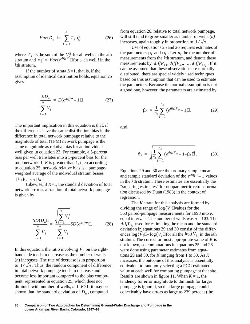
,
off
llysatenot by
sea-
rdr-
e.
(26)
where is the sum of the for all wells in thekthstratum and for each welli in thekth stratum.
If the number of strataK=1, that is, if theassumption of identical distribution holds, equation 25gives
. (27)
The important implication in this equation is that, ifthe differences have the same distribution, bias in thedifference in total network pumpage relative to themagnitude of total (TFM) network pumpage is thesame magnitude as relative bias for an individualwell given in equation 22. For example, a 5-percentbias per well translates into a 5-percent bias for thetotal network. IfK is greater than 1, then accordingto equation 25, network relative bias is a pumpage-weighted average of the individual stratum biases
.Likewise, if K=1, the standard deviation of total
network error as a fraction of total network pumpageis given by
. (28)
In this equation, the ratio involving on the right-hand side tends to decrease as the number of wells(n) increases. The rate of decrease is in proportionto . Thus, the random component of differencein total network pumpage tends to decrease andbecome less important compared to the bias compo-nent, represented in equation 25, which does notdiminish with number of wells,n. If K>1, it may beshown that the standard deviation of , computed
from equation 26, relative to total network pumpagewill still tend to grow smaller as number of wells (n)increases, again roughly in proportion to .
Use of equations 25 and 26 requires estimatesthe parameters and . Let be the number omeasurements from thekth stratum, and denote thesemeasurements by . If itcan be assumed that these observations are normadistributed, there are special widely used techniquebased on this assumption that can be used to estimthe parameters. Because the normal assumption is a good one, however, the parameters are estimated
. (29)
and
. (30)
Equations 29 and 30 are the ordinary sample meanand sample standard deviation of the valuein thekth stratum. These estimates are essentially th“smearing estimates” for nonparametric retransformtion discussed by Duan (1983) in the context ofregression.
TheK strata for this analysis are formed bydividing the range of values for the553 paired-pumpage measurements for 1998 intoKequal intervals. The number of wells wasn = 103. The
used for estimating the mean and the standadeviation in equations 29 and 30 consist of the diffeences for all the in thekthstratum. The correct or most appropriate value ofK isnot known, so computations in equations 25 and 26were done using parameter estimates from equa-tions 29 and 30, forK ranging from 1 to 50. AsKincreases, the outcome of this analysis is essentiallyequivalent to randomly selecting a PCC-estimatedvalue at each well for computing pumpage at that sitResults are shown in figure 11. WhenK = 1, thetendency for error magnitude to diminish for largerpumpage is ignored, so that large pumpage couldconceivably have errors as large as 239 percent (the
Var Dn( ) Tkσk2
k 1=
K
∑=
Tk Vi2
σk2 Var ediffPi( )=
EDn
Vi
i 1=
n
∑-------------- E ediffP 1–( )=
µ1 µ2 … µK, , ,
SD Dn( )
Vi
i 1=
n
∑-------------------
Vi2
i 1=
n
∑
Vi
i 1=
n
∑--------------------SD ediffP( )=
Vi
1 n⁄
Dn
1 n⁄
µk σk nk
diffPk1 diffPk2 … diffPknk, , ,
µk1nk----- ediffPkj 1–( )
j 1=
nk
∑=
σk1nk----- ediffPkj 1 µk––( )2
j 1=
nk
∑=
ediffP 1–
Vi( )log
diffPkj
Vi( ) Vi( )log–log Vi( )log
36 Comparison of Two Approaches for Determining Ground-Water Discharge and Pumpage in theLower Arkansas River Basin, Colorado, 1997–98

s
ga-
maximum value in the data set; see fig. 9A), an errorthat, in the actual data set, is associated with a wellthat contributes little to total network pumpage. Theresults of permitting large errors to be associated withwells having large pumpage are severe, yielding amean of about 9.3 percent and standard deviation ofabout 11.9 percent forK = 1 (fig. 11). ForK = 2, themean decreases to 2.70 percent; forK = 3, it decreasesto 0.77 percent; for K = 4, it decreases to less than0 percent; forK greater than about 10, the mean tendsto level off at approximately−0.91 percent. Likewise,
the standard deviation levels off forK greater than 4 atabout 1.25 percent. The fact that the mean becomenegative whenK is greater than 4 indicates that thelarge positive errors at a small number of wells havelittle effect on total network pumpage; it is instead theinfluence of negative errors for large-pumpage wells(see figure 9) that is causing the mean to become netive asK increases. Imposing the restriction thatnumber of strataK be larger than 4 prevents the fewvery large positive errors from being associated withwells that have large pumpage.
ESTIMATION OF TOTAL NETWORK PUMPAGE 37
0 550 5 10 15 20 25 30 35 40 45 50
NUMBER OF STRATA
-2
13
-2
-1
0
1
2
3
4
5
6
7
8
9
10
11
12
PE
RC
EN
T
Standard deviation
Mean
Figure 11. Graph showing relation of the mean and standard deviation of total network pumpage, in percent, tothe number of strata.

s
ri-
t’sts
e
97
ss
fi-asdr-r-,if--
cy
.
The approximate normality of the difference innetwork-aggregated pumpage can be used withthe mean and the standard deviation to make proba-bility statements about likely differences in totalnetwork pumpage obtained by TFM and PCCapproach. Using a mean of−0.91 percent and a stan-dard deviation of 1.25 percent, for example, resultsin a conclusion that, for any given year, there is a95-percent probability that the difference in aggre-gated pumpage between the TFM and PCC approachwould be between about−3.41 and 1.59 percent for anetwork of 103 wells.
To predict the difference in aggregated pumpagefor a larger network, the distribution of total TFMpumpage (the values of ) will be assumed to be thesame, the estimate of the mean remains the same(−0.91 percent), but the standard deviation decreasesin proportion to the square root of the ratio of numbersof wells. Forn = 1,000 wells, the 1.25 percent standarddeviation for 103 wells decreases by a factor of ,resulting in an estimated standard deviation of0.40 percent. Therefore, for a network of 1,000 wells,there is a 95-percent probability that the difference inaggregated pumpage between the TFM and the PCCapproach for any given year would be between−1.71and−0.11 percent.
CONCLUSIONS
This report compares two approaches fordetermining instantaneous ground-water dischargeand pumpage. The data collected and analyzed aspart of this study included (1) logarithmically trans-formed differences of well discharge computed from747 paired discharge measurements made at 105 wellsduring 1997 and 1998; (2) power conversion coeffi-cients (PCC’s) derived for 104 wells during 1997and 1998; (3) ranked, logarithmically transformeddifferences of pumpage computed from 553 pairedpumpage comparisons made at 103 wells during 1998,and (4) State-approved PCC’s that were made from1994–97.
Given the data analysis presented in this report,the main conclusions are:1. More than 80 percent of the differences in
well discharge were less than 10 percent. Theoverall mean difference in well discharge for allsites was 0.0 percent, indicating no differenceon average between TFM’s and portable flow-meter instantaneous discharge measurements.
For varying site characteristics, mean differencein well discharge range from a−4 percent to4 percent.
2. Variations in PCC’s measured during the 1998 irgation season indicated that 58 percent of thewells had less than 10-percent change, and86 percent of the wells had less than 20-percenchange. Systematic seasonal variations in PCCgenerally were not evident for the measuremenmade during the 1998 irrigation season.
3. Ninety percent of the sites had at least one PCCmeasured during 1997 that was less than therange of PCC’s measured in 1998, indicating thrange in PCC’s measured at majority of sitesbetween 1997 and 1998 were similar.
4. About 48 percent of the State-approved PCC’smade between 1994 through 1997 were within10 percent of the 1998 site average PCC’s andabout 67 percent of the State-approved PCCmeasurements made between 1994 through 19were within 20 percent of the 1998 site averagePCC’s.
5. About 80 percent of the differences in pumpagebetween the TFM and PCC approaches were lethan 10 percent. The overall mean difference inpumpage was 0.01 percent, indicating no signicant difference on average between pumpage measured by TFM’s and pumpage as computeby the PCC approach. For varying site characteistics, mean differences in pumpage were geneally less than±3 percent and, for most instancesthe mean differences in pumpage were not signicantly different from zero at the 5-percent significance level.
6. There are several potential sources of discrepanbetween pumpage as measured by a TFM andpumpage as computed by the PCC approach.With data currently available, it is not possibleto give reliable estimates of the magnitude ofeach of the potential sources of pumpage errorHowever, using available data, an estimate oferrors caused by temporal variability of PCC’scan be made. The year-to-year variance wasabout nine times the date-within-year variance,indicating that year-to-year variability of thePCC’s may make a significant contribution toerror in the PCC approach for estimatingpumpage. This conclusion is based on anassumption that the State-approved PCC’sfrom 1994–97 are of the same quality as the1998 PCC’s.
Dn
Vi
1031000−−−−−−−
38 Comparison of Two Approaches for Determining Ground-Water Discharge and Pumpage in theLower Arkansas River Basin, Colorado, 1997–98

a-
al
3]
r
--
an
7. For a network of 103 wells and a number of strata(logarithms of TFM total pumpage divided intoequal subdivisions) greater than 10, the resultingmean and standard deviation indicates that, forany given year, there is a 95-percent probabilitythat the difference in aggregated pumpagebetween the TFM and PCC approach would bebetween about−3.41 and 1.59 percent.
8. The difference in aggregated pumpage would beexpected to be smaller as the number of well sitesbecomes larger. Assuming the distribution oftotal TFM pumpage is the same for 1998 data set,there is a 95-percent probability that the differ-ence in aggregated pumpage between the TFMand the PCC approach, for any given year, for anetwork of 1,000 wells would be between−1.71and−0.11 percent. This assumes that the largedifferences in pumpage are confined to wellswith smaller pumpage. It also is important toemphasize that only 1998 pumpage data wereused for this analysis, so the effect of temporalvariations of PCC’s on total network pumpage isnot known.
REFERENCES CITED
Duan, Naihua, 1983, Smearing estimate—A nonparametricretransformation method: Journal of the AmericanStatistical Assoc., v. 78, no. 383, p. 605–610.
Graybill, F.A., 1976, Theory and application of the linearmodel: Belmont, Calif., Wadsworth Publishing Co.,704 p.
Helsel, D.R., and Hirsch, R.M., 1992, Statistical methods inwater resources: New York, Elsevier, Studies in Envi-ronmental Science 49, 522 p.
Hora, S.C. and Iman, R.L., 1988, Asymptotic relativeefficiencies of the rank-transformation procedurein randomized complete block designs, Journal ofthe American Statistical Assoc., v. 83, no. 402,p. 462–470.
Hurr, R.T., and Litke, D.W., 1989, Estimating pumping timeand ground-water withdrawals using energy consump-tion data: U.S. Geological Survey Water-ResourcesInvestigations 89–4107, 27 p.
Iman, R.L,. and Conover, W.J., 1981, Rank transforma-tions as a bridge between parametric and nonpara-metric statistics: American Statistician, v. 35, no. 3,p. 124–129.
Kepner, J.L. and Wackerly, D.D., 1996, On rank transformtion techniques for balanced incomplete repeatedmeasures designs: Journal of the American StatisticAssoc., v. 91, no. 436, p. 1619–1625.
Litke, D. W., and Appel, C.L., 1989, Estimated use ofwater in Colorado, 1985: U.S. Geological SurveyWater-Resources Investigations 88–4101, 157 p.
Luckey, R. R., 1972, Analyses of selected statisticalmethods for estimating groundwater withdrawal:Water Resources Research, v. 8, no. 1, p. 205–210.
Office of the State Engineer, 1994, Rules governing themeasurement of tributary ground water diversionslocated in the Arkansas River Basin: Denver, 4 p.(dated July 6, 1994) [Unpublished report available onfile at the Office of the State Engineer, Division ofWater Resources, Colorado Department of NaturalResources, 1313 Sherman Street, Denver, CO 8020
Office of the State Engineer, 1996, Amendments to rulesgoverning the measurement of tributary ground watediversions located in the Arkansas River Basin:Denver, 6 p. (dated February 28, 1996) [Unpublishedreport available on file at the Office of the State Engineer, Division of Water Resources, Colorado Department of Natural Resources, 1313 Sherman Street,Denver, CO 80203]
Omega Engineering, Inc., 1992, Complete flow and levelmeasurement handbook and encyclopedia: v. 28,Stanford, Conn.,
Scott, J. C., 1990, Computerized stratified random site-selection approaches for design of a ground-water-quality sampling network: U.S. Geological SurveyWater-Resources Investigations 90–4101, 109 p.
Snedecor, G.W., and Cochran, W.G., 1967, Statisticalmethods (6th ed.), Ames, Iowa State UniversityPress
Tornqvist, Leo; Vartia, Pentti, and Vartia, Yrjo O., 1985,How should relative changes be measured?: AmericStatistician, v. 39, no. 1, p. 43–46.
REFERENCES CITED 39