computational fluid dynamics (cfd) of vehicle … development of the cfd model consists of first...
TRANSCRIPT
COMPUTATIONAL FLUID DYNAMICS (CFD) OF VEHICLE
AERODYNAMICS AND ASSOCIATED ACOUSTICS
A thesis submitted in accordance with the regulations for the
degree of Doctor of Philosophy
By
Nurul Muiz Murad
School of Engineering and Industrial Science
Swinburne University of Technology, Melbourne, Australia
February, 2009

ABSTRACT Vortex generation behind the A-pillar region due to airflow separation leads to
aero-acoustics generation. The magnitude and intensity of the vortex and hence
aero-acoustics activities are further enhanced when vehicle are exposed to
crosswind especially when travelling on a highway. The objective of this project
is to develop a computational fluid dynamic (CFD) and computational aero-
acoustics (CAA) model to best simulate aerodynamic flow and aero-acoustics
propagation behind the A-pillar region of simplified vehicle with varying
windshield radii under various yaw conditions. The CFD model will then be used
to investigate and better understand the aerodynamic and aero-acoustics
distribution behaviour surrounding area of the vehicle A-pillar region. The
simplified vehicle model used was of 40% scale. Models investigated consist of
three models of different circular windshield/A-pillar radii and two models of with
sharp A-pillar edges with different windshield slant angle. Models used in this
project were subjected to 0°, 5°, 10° and 15° yaw angles. The models were
modelled under laboratory conditions, exposed to boundary inlet velocities of 60,
100 and 140 km/h.
The development of the CFD model consists of first investigating and selecting
the best grids configurations for both the circular and sharp edge A-pillar models
at various respective yaw angles. The process was then to select the best
turbulence and near wall model for the CFD model. The grids, turbulence and
near wall models selected for comparison were investigated from commercial
CFD software’s FLUENT and SWIFT AVL. The final stage in the development
of the numerical model was to develop a CAA model for the aero-acoustics
modelling. The final grid configuration selected for the CFD models in this
project was the polyhedral grids from SWIFT. The final selection of turbulence
and near wall model selected was the standard k – ε turbulence model and the near
wall model of Chieng and Launder (1980) for the circular models at 0° yaw. For
all the other models at various yaw angles, the turbulence and near wall model of
choice was the RSM with the WEB near wall model. Validation of the final CFD
model against the experimental data of Alam (2000) resulted in good correlations.
ii

The CAA model developed for this project was conducted using SWIFT CAA and
was conducted only for the circular models due to their better correlations with
experimental data.
From the CFD and CAA numerical models developed, investigation was then
conducted in determining the source and mechanism of vortex generation behind
the A-pillar and the overall physical shape and turbulence flow characteristics of
the A-pillar vortex itself. The CAA investigation focused in determining the
transient behaviour of the models and also the acoustical behaviour on the A-pillar
surface and surrounding region.
The results obtained from the CFD analysis shows that the source of vortex
separation behind the A-pillar region originated from the junction of the A-pillar
base, the A-pillar apex and the front side window and roof junction. The
mechanism of flow separation was due to trailing edge separation. The shape of
the vortices that takes place took a physical form of either a two-dimensional
quasi-elongated oval, a mixture of two and three-dimensional mixture of a quasi
circular and cone shaped helical vortex or a three-dimensional vertically elongated
cone shape helical vortex propagating downstream to the flow. The various
geometrical configurations of the windshield radii and slant angle determined the
vortex size, magnitude and intensity behind the A-pillar region when exposed to
yawed or un-yawed position.
Hybrid SWIFT CAA results showed good correlation when compared to results
obtained by Alam (2000). The transient progression for each investigated scale
model shows that the circular and sharp edge models investigated will reach a
faster steady state condition with increasing windshield radii and when exposed to
un-yawed condition due to a reduced turbulent activities behind the A-pillar
region. Results show that the OASPL magnitude is higher on vehicle subjected to
yawing conditions. Results also show that OASPL magnitude on the vehicle
surface decreases with increases windshield radii. The aerodynamic noise
generation decreases as it moves away from the vehicle surface. Overall, mean
surface OASPL magnitude at the vortex source region (A-pillar Base Junction, A-
pillar apex and Roof) is slightly higher compared to the overall mean OASPL
magnitude on the surface of the vehicle.
iii

ACKNOWLEDGEMENTS
Bismillah-ir Rahman-ir Rahim, Alhamdulillah syukur ke hadrat Allah s.w.t.
kerana dengan limpah dan kurnia-Nya akhirnya dapat juga saya menghabiskan
thesis ini.
Saya ingin mengambil kesempatan ini untuk mengucapkan ribuan terima kasih
yang tidak terhingga buat kedua ibu bapa saya, Haji Murad bin Haji Ahmad dan
Hajjah Alisma binti Haji Sarudin. Berdirinya saya pada hari ini sebagai seorang
manusia yang sempurna adalah berkat doa serta hasil usaha mereka membimbing
dan memberi tunjuk ajar kepada saya.
Al-Fatihah buat Allahyarhammah Hajjah Daimah binti Haji Daud, moyang saya
yang bersusah payah menjaga saya semasa kecil. Semoga rohnya sentiasa dicucuri
rahmat. Amin.
Terima kasih yang tidak terhingga buat nenek saya, Hajjah Sabedar binti Haji
Abdul Munaf dan makandak saya, Hajjah Siti Harani binti Haji Sarudin. Saya
tidak akan dapat membalas jasa mereka menjaga dan mendidik dari kecil
sehinggalah dewasa. Terima kasih juga buat pakcik serta makcik saya, Pak Long
dan Mak Long, Pak Gadang dan Mak Gadang, Pak Ngah dan Mak Ngah, Pak
Lang dan Mak Lang, Pak Uteh dan Mak Uteh, Pak Anjang dan Mak Anjang serta
Pak Kecik dan Mak Kecik. Kasih sayang serta tunjuk ajar mereka sedikit
sebanyak mencorak perwatakan saya pada hari ini.
Terima kasih buat adik-adik saya, Nur Meliza binti Haji Murad, Nurul Muhriz bin
Haji Murad dan Nurul Mahfuz bin Haji Murad. Hadir mereka dalam hidup saya
telah memberi saya perangsang untuk terus maju dan menjadi yang terbaik buat
contoh untuk mereka ikuti. Tidak lupa juga, saya tujukan kejayaan saya buat
sepupu-sepupu saya serta rakan-rakan saya di seluruh Malaysia dan Australia
terutamanya rakan-rakan lama di MTD, AUSMAT dan Dewan Malaysia.
Terima kasih buat supervisor saya Dr. Jamal Naser dan Dr. Simon Watkins.
Terutama buat Dr. Jamal Naser yang telah memberi kepercayaan, motivasi serta
iv

bimbingan buat saya untuk menghabiskan thesis ini. Dr. Jamal Naser bukan sahaja
menjadi supervisor malah mentor dan kawan baik saya.
Terima kasih buat rakan seperjuangan saya, Dr. Firoz Alam, Dr. James Hart dan
Dr. Gregory Chawynski yang telah menolong saya dan membimbing saya
sepanjang perjuangan saya menyiapkan thesis ini.
Tidak lupa, setinggi-tinggi penghargaan dan ucap terima kasih buat mentor dan
rakan baik saya di Melbourne, Encik Ahmad Fuad Mansor yang telah berada
disisi saya disaat susah dan senang. Pertolongan, nasihat serta bimbingan beliau
akan saya kenang sampai bila-bila.
Terima kasih buat kerajaan Malaysia yang telah menaruh kepercayaan kepada
saya dengan menghantar saya ke bumi Australia untuk melanjutkan pelajaran
dalam peringkat sarjana muda. Tanpa inisiatif dari mereka, semua ini tidak akan
menjadi kenyataan.
Akhir sekali, terima kasih saya ucapkan buat saudari Jasmin binti Mohd Ramli
yang sentiasa menjadi sumber inspirasi saya dalam mengharungi ranjau hidup
yang penuh mencabar.
Nurul Muiz Murad
Ogos 2008
v
DECLARATION OF ORIGINALITY
I, Nurul Muiz Murad, hereby declare that this thesis contains no material, which
has been accepted for the award of any other degree or diploma in any university
or institute of education. To the best of my knowledge and belief, no material in
this thesis has been previously published or written by another person except
where due references is made in the body of the thesis.
Signed ………………………………….
Nurul Muiz Murad
August, 2008
vi

TABLE OF CONTENTS
Abstract ii
Acknowledgements iv
Declaration of Originality vi
Table of Contents vii
List of Figures xi
List of Tables xxiii
Nomenclature xxv
List of Abbreviations and Acronyms xxvii
Chapter One: Introduction & Literature Review 1
1.1 History of Vehicle Aerodynamics: A General Background 1 1.2 Airflow around a Ground Vehicle 2 1.3 Overview on Sound and Noise 6 1.4 Problems associated with Vehicle Vortex Flow 10 1.5 Vehicle Noise 13 1.6 Mechanism of Aerodynamic Generation 16 1.7 Ways of Reducing A-Pillar Aerodynamic Noise 22 1.8 Vehicle Aerodynamics and Aeroacoustics: Numerical and
Computational Evaluation Methods 24 1.9 Literature Review on A-Pillar Aerodynamics and Aeroacoustics 27 1.10 Conclusions and Evaluation from Previous Research Work 38 1.11 Research Project Motivation, Scope and Proposed Methodology 42 1.12 Objectives of PhD Project 43 1.13 Thesis Layout 44
Chapter Two: Governing Equations and Boundary Conditions 46
2.1 Turbulence and Early Works of Turbulence Modelling 46 2.2 Governing Transport Equation and Turbulence Models 48 2.3 Algebraic (zero equation) Turbulence Models 51 2.4 One Equation Turbulence Models 52 2.5 Two Equation Turbulence Models 54 2.6 Deficiencies of the Two Equation Turbulence Model 63
2.6.1 Pressure Gradient Effects 63 2.6.2 Effect of Rapid change of Mean Strain Rate and Streamline
Curvature 64 2.7 Reynolds Stress Turbulence Models 65 2.8 Direct Numerical and Large Eddy Simulation 73
vii
2.9 CFD Near Wall Treatment and Boundary Conditions 75 2.10 Wall Function Approach 76 2.11 Low Reynolds Number Model approach 80 2.12 Boundary Conditions 83 2.13 Computational Aeroacoustics 85 2.14 Lighthill Acoustic Analogy Method 86 2.15 Kirchoff Method 88 2.16 Perturbation Method 88 2.17 Linearized Euler Equation Method 89
Chapter Three: Methodology 98
3.1 General CFD Approach Process 98 3.2 Accuracy Factors and Errors Associated with CFD 99 3.3 CFD Grid Generation and Discretization Methods 101 3.4 CFD Numerical Schemes 106 3.5 Segregated and Coupled Solver 110 3.6 Near Wall Models and Turbulence Models 111 3.7 CAD Model Geometry and Boundary Conditions Input 115
Chapter Four: RANS CFD of A-Pillar Aerodynamics 123
4.1 Objective and Scope of this Chapter 123 4.2 CFD Model Development 124
4.2.1 Grid Feasibility Study – Generation Technique 124 4.2.2 Grid Feasibility Study – 131
Grid Refinement & Independency Procedure 4.2.3 Grid Feasibility Study – 137
Validation with Experimental Results at 0° Yaw 4.2.4 Near Wall Model and Turbulence Model Feasibility Study 143
4.2.4.1 Circular Models at 0° Yaw - 143 Near Wall Model and Turbulence Model Feasibility Study
4.2.4.2 Circular Models at 5°, 10° and 15º Yaw – 146 Near Wall Model and Turbulence Model Feasibility Study
4.2.4.3 Sharp Edge Models at 0°, 5°, 10° and 15º Yaw – 158 Near Wall Model and Turbulence Model Feasibility Study
4.3 Circular Models at 0º Yaw – Results and Discussion 165 4.4 Circular Models at 5° yaw – Results and Discussion 171 4.5 Circular Models at 10° and 15° Yaw – Results and Discussion 178 4.6 RE Model at 0° Yaw – Results and Discussion 189 4.7 SL Model at 0° Yaw – Results and Discussion 193 4.8 RE Model at 5°, 10° and 15° Yaw – Results and Discussion 199 4.9 Slanted Model at 5°, 10° and 15° Yaw – Results and Discussion 206 4.10 General Discussion 213
viii

Chapter Five: Computational Aeroacoustics (CAA) Simulations 221
5.1 Introduction to the Hybrid SWIFT CAA Approach 221 5.2 Methodology of the Hybrid SWIFT CAA Approach 223 5.3 Objectives & Scope of using Hybrid SWIFT CAA Approach: 228
Application to this Research Project 5.3.1 Objectives of Chapter 5 229 5.3.2 Scope of Chapter 5 230
5.4 Hybrid SWIFT CAA Results 231 5.4.1 Hybrid SWIFT CAA & Experimental Validation - 231
SE Model, 0° & 15° Yaw 5.4.2 Hybrid SWIFT CAA & Experimental Validation - 235
Semi Model, 0° & 15° Yaw 5.4.3 Hybrid SWIFT CAA & Experimental Validation – 239
LE Model, 0° & 15° Yaw 5.4.4 Hybrid SWIFT CAA & Experimental Validation – 243
RE Model, 0° & 15° Yaw 5.4.5 Hybrid SWIFT CAA & Experimental Validation – 247
SL Model, 0° & 15° Yaw 5.4.6 Aeroacoustics Behaviour during Transient Condition – 252
SE Model, 0° & 15° Yaw 5.4.7 Aeroacoustics Behaviour during Transient Condition – 254
Semi Model, 0° & 15° Yaw 5.4.8 Aeroacoustics Behaviour during Transient Condition – 255
LE Model, 0° & 15° Yaw 5.4.9 Aeroacoustics Behaviour during Transient Condition - 257
RE Model, 0° & 15° Yaw 5.4.10 Aeroacoustics Behaviour during Transient Condition – 258
SL Model, 0° & 15° Yaw 5.4.11 CAA Behaviour & Distribution behind A-pillar Region – 260
SE Model, 0° Yaw 5.4.12 CAA Behaviour & Distribution Behind A-pillar Region – 265
SE Model, 15° Yaw 5.4.13 CAA Behaviour & Distribution Behind A-pillar Region – 270
Semi Model, 0° Yaw 5.4.14 CAA Behaviour & Distribution Behind A-pillar Region – 275
Semi Model, 15° Yaw 5.4.15 CAA Behaviour & Distribution Behind A-pillar Region – 280
LE Model, 0° Yaw 5.4.16 CAA Behaviour & Distribution Behind A-pillar Region – 285
LE Model, 15° Yaw 5.5 Discussion of Hybrid SWIFT CAA Results 291
5.5.1 Comparison between Hybrid SWIFT CAA & 291 Experimental Results – Cp RMS Pressure
5.5.2 Comparison between Hybrid SWIFT CAA & 294 Experimental Results – PSD Distribution
5.5.3 Aero-acoustics Behaviour during Transient Conditions 298 5.5.4 CAA Behaviour Behind the A-pillar Region 300
ix
Chapter Six: Conclusions & Recommendations 306
6.1 Conclusions from Chapter 4 306 6.2 Conclusions from Chapter 5 310 6.3 Further Recommendations 313
References 315 Bibliography 330
x

LIST OF FIGURES
Figure 1.1. Areas of Separation around a Vehicle 4
Figure 1.2. Slanted A-pillar Vortex flow 5
Figure 1.3. High Pressure Zone in a Vortex Flow behind a Backward-Facing 7
Step
Figure 1.4. Fletcher Munsen Curve 8
Figure 1.5. Forced and Free Vortex Velocity Distribution 11
Figure 1.6. Two method of Leak Noise Transmission 18
Figure 1.7. Mechanism of Cavity Noise Transmission 20
Figure 1.8. Wind Rush Noise Transmission around Vehicle 22
Figure 3.1: Simplified Vehicle Model Geometry with Varying 116
A-pillar Windshield Radius
Figure 3.2: Figure 3.2: Models in 0°, 5°, 10° and 15° yaw position 117
Figure 3.3: Small Ellipsoidal Model in a yaw position within 117
Computational Domain in AVL
Figure 3.4: Slanted Edge Model within Computational Domain in FLUENT 118
Figure 3.5: Semi Circular Model within Computational Domain in AVL 119
Figure 3.6: Slanted Edge Model with Multi-block volumes in GAMBIT 119
Figure 4.1: Slanted Edge Model with Multi-block volumes in GAMBIT 125
Figure 4.2: Fully Structured Hexahedral Grids Layout in GAMBIT 126
Figure 4.3: Grid Skewness Quality of the Fully Structured Hexahedral 126
Grids in GAMBIT
Figure 4.4: Hybrid Grids Layout in GAMBIT 127
Figure 4.5: Grid Skewness Quality of the Hybrid Grids in GAMBIT 128
Figure 4.6: Unstructured Tetrahedral Grids Layout in GAMBIT 128
Figure 4.7: Grid Skewness Quality of the Unstructured Tetrahedral 129
Grids in GAMBIT
Figure 4.8: ACT Polyhedral Grids Layout in AVL generated using 130
Fame Hybrid
Figure 4.9: Before and After Solution Adaptive Refinement for 133
Semi Circular Model meshed with unstructured Tetrahedral
xi
Grids in GAMBIT
Figure 4.10: Boundary Layer Grids for the Slanted Edge Model 134
generated using the Hybrid Grids Method in GAMBIT
Figure 4.11: Grid Independency Test for the Semi Circular Model in 135
AVL at 0° Yaw
Figure 4.12: Grid Independency Test for the Semi Circular Model in 136
AVL at 15° Yaw
Figure 4.13: Grid Independency Test Results for the Semi Circular 138
Model in FLUENT at 0° Yaw
Figure 4.14: Grid Independency Test Results for the Semi Circular 138
Model in AVL at 0° Yaw
Figure 4.15: Comparison between Hexahedral, Hybrid and Tetrahedral 139
Grid Generation Method in FLUENT at 0° Yaw
Figure 4.16: Grid Independency Test Results for the Slanted Edge Model in 140
AVL at 0° Yaw with Standard Wall Function
Figure 4.17: Comparison between Hybrid and Polyhedral Grids at High and 141
Low Reynolds Number Conditions
Figure 4.18: SE Model, 0° Yaw 144
Figure 4.19: Semi Model, 0° Yaw 145
Figure 4.20: LE Model, 0° Yaw 145
Figure 4.21: SE Model, 5° Yaw, Bottom Row, Turbulence Model 147
Comparison
Figure 4.22: SE Model, 10° Yaw, Bottom Row, Turbulence Model 147
Comparison
Figure 4.23: SE Model, 15° Yaw, Bottom Row, Turbulence Model 148
Comparison
Figure 4.24: Semi Model, 5° Yaw, Bottom Row, Turbulence Model 149
Comparison
Figure 4.25: Semi Model, 10° Yaw, Bottom Row, Turbulence Model 149
Comparison
Figure 4.26: Semi Model, 15° Yaw, Bottom Row, Turbulence Model 150
Comparison
xii

Figure 4.27: LE Model, 5° Yaw, Bottom Row, Turbulence Model 151
Comparison
Figure 4.28: LE Model, 10° Yaw, Bottom Row, Turbulence Model 151
Comparison
Figure 4.29: LE Model, 15° Yaw, Bottom Row, Turbulence Model 152
Comparison
Figure 4.30: SE Model, 5° Yaw, Bottom Row, RSM-WEB Turbulence 153
Model
Figure 4.31: SE Model, 10° Yaw, Bottom Row, RSM-WEB Turbulence 153
Model
Figure 4.32: SE Model, 15° Yaw, Bottom Row, RSM-WEB Turbulence 154
Model
Figure 4.33: Semi Model, 5° Yaw, Bottom Row, RSM-WEB Turbulence 155
Model
Figure 4.34: Semi Model, 10° Yaw, Bottom Row, RSM-WEB Turbulence 155
Model
Figure 4.35: Semi Model, 15° Yaw, Bottom Row, RSM-WEB Turbulence 156
Model
Figure 4.36: LE Model, 5° Yaw, Bottom Row, RSM-WEB Turbulence 156
Model
Figure 4.37: LE Model, 10° Yaw, Bottom Row, RSM-WEB Turbulence 157
Model
Figure 4.38: LE Model, 15° Yaw, Bottom Row, RSM-WEB Turbulence 157
Model
Figure 4.39: SL Model, 0° Yaw, Bottom Row, Turbulence Model 159
Comparison
Figure 4.40: SL Model, 0° Yaw, Top Row, Turbulence Model 159
Comparison
Figure 4.41: SL Model, 0° Yaw, Bottom Row, Turbulence Model 160
Comparison
Figure 4.42: SL Model, 0° Yaw, Top Row, Turbulence Model 161
Comparison
xiii

Figure 4.43: Slanted Edge Model, 5° Yaw, Bottom Row, RSM-WEB 162
Turbulence Model
Figure 4.44: Slanted Edge Model, 10° Yaw, Bottom Row, RSM-WEB 162
Turbulence Model
Figure 4.45: Slanted Edge Model, 15° Yaw, Bottom Row, RSM-WEB 163
Turbulence Model
Figure 4.46: Rectangular Model, 0° Yaw, Bottom Row, RSM-WEB 163
Turbulence Model
Figure 4.47: Rectangular Model, 5° Yaw, Bottom Row, RSM-WEB 164
Turbulence Model
Figure 4.48: Rectangular Model, 10° Yaw, Bottom Row, RSM-WEB 164
Turbulence Model
Figure 4.49: Rectangular Model, 15° Yaw, Bottom Row, RSM-WEB 165
Turbulence Model
Figure 4.50: SE Model, 0° Yaw, External Surface Streamline, Front View 166
Figure 4.51: SE Model, 0° Yaw, External Surface Streamline, Top View 166
Figure 4.52: SE Model, 0° Yaw, Top View, Turbulent Velocity 168
Figure 4.53: SE Model, 0° Yaw, Front View, Velocity Vector 168
Figure 4.54: SE Model, 0° Yaw, Surface Streamline 169
Figure 4.55: SE Model at 0° Yaw, Surface Streamline Visualisation 170
using Wool Tuffs (after Alam, 2000)
Figure 4.56: Semi Model, 0° Yaw, Top View, Turbulent Velocity 170
Figure 4.57: LE Model, 0° Yaw, Top View, Turbulent Velocity 171
Figure 4.58: SE Model, 5° Yaw, Leeward Region, External Flow 172
Streamline
Figure 4.59: SE Model, 5° Yaw, Windward Region, External Flow 172
Streamline
Figure 4.60: Semi Model, 5° Yaw, Front View, External Flow Streamline 173
Figure 4.61: LE Model, 5° Yaw, Front View, External Flow 174
Streamline
Figure 4.62: SE Model, 5° Yaw, Front View, Velocity Vector 175
Figure 4.63: SE Model, 5° Yaw, Top View, Turbulent Velocity 176
xiv
Figure 4.64: SE Model, 5º Yaw, Reynolds Stresses Component, 177
Leeward and Windward Region of the A-pillar
Figure 4.65: SE Model, 10° Yaw, Front View, External Surface 179
Streamline
Figure 4.66: SE Model, 15° Yaw, Leeward View, External Surface 179
Streamline
Figure 4.67: Semi Model, 10° Yaw, Front View, External Surface 180
Streamline
Figure 4.68: LE Model, 10° Yaw, Front View, External Surface 181
Streamline
Figure 4.69: Semi Model, 15° Yaw, Front View, External Surface 182
Streamline
Figure 4.70: LE Model, 15° Yaw, Front View, External Surface 182
Streamline
Figure 4.71: SE Model, 15° Yaw, Leeward Region, Surface Flow 183
Streamline
Figure 4.72: SE Model at 15° Yaw in the Leeward Region, Surface 183
Streamline Visualisation using Wool Tuffs (after Alam, 2000)
Figure 4.73: SE Model, 15° Yaw, Windward Region, Surface Flow 184
Streamline
Figure 4.74: SE Model at 15° Yaw in the Windward Region, Surface 184
Streamline Visualisation using Wool Tuffs (after Alam, 2000)
Figure 4.75: SE Model, 10° Yaw, Top View, Turbulent Velocity 185
Figure 4.76: SE Model, 10° Yaw, Front View, Velocity Vector 185
Figure 4.77: SE Model, 15° Yaw, Top View, Turbulent Velocity 186
Figure 4.78: SE Model, 15° Yaw, Front View, Velocity Vector 186
Figure 4.79: SE Model, 10º Yaw, Reynolds Stresses Component, 187
Leeward and Windward Region of the A-pillar
Figure 4.80: SE Model, 15º Yaw, Reynolds Stresses Component, 188
Leeward and Windward Region of the A-pillar
Figure 4.81: Rectangular Model, 0° Yaw, Front View, External Flow 189
Streamline
xv

Figure 4.82: Rectangular Model, 0° Yaw, Side View, Surface 190
Streamline
Figure 4.83: RE Model at 0° Yaw, Surface Streamline Visualisation 190
using Wool Tuffs (after Alam, 2000)
Figure 4.84: Rectangular Model, 0° Yaw, Turbulence Velocity 191
Contour Distribution
Figure 4.85: Rectangular Model, 0° Yaw, Front View, UU Reynolds 192
Stress Component
Figure 4.86: Rectangular Model, 0° Yaw, Front View, VV Reynolds 192
Stress Component
Figure 4.87: Rectangular Model, 0° Yaw, Front View, WW Reynolds 193
Stress Component
Figure 4.88: Slanted Edge Model, 0° Yaw, Front View, External Flow 194
Streamline
Figure 4.89: Slanted Edge Model, 0° Yaw, Side View, Surface Flow 195
Streamline
Figure 4.90: SL Model at 0° Yaw, Surface Streamline Visualisation 196
using Wool Tuffs (after Alam, 2000)
Figure 4.91: Slanted Edge Model, 0° Yaw, Turbulence Velocity 196
Contour Distribution
Figure 4.92: Slanted Edge Model, 0° Yaw, Front Plane View, Velocity 197
Vector Distribution
Figure 4.93: Slanted Edge Model, 0° Yaw, Front View, UU Reynolds 198
Stress Component
Figure 4.94: Slanted Edge Model, 0° Yaw, Front View, VV Reynolds 198
Stress Component
Figure 4.95: Slanted Edge Model, 0° Yaw, Front View, WW Reynolds 199
Stress Component
Figure 4.96: Rectangular Model, 5° Yaw, Frontal External 200
Streamline Airflow
Figure 4.97: Rectangular Model, 10° Yaw, Frontal External 201
Streamline Airflow
xvi

Figure 4.98: Rectangular Model, 15° Yaw, Frontal External 202
Streamline Airflow
Figure 4.99: Rectangular Model, 15° Yaw, Turbulent Velocity 202
Figure 4.100: Rectangular Model, 15° Yaw, Leeward Surface 203
Streamline Airflow
Figure 4.101: RE Model at 15° Yaw in the Leeward Region, 204
Surface Streamline Visualisation using Wool
Tuffs
Figure 4.102: Rectangular Model, 15° Yaw, Windward Surface 205
Streamline Airflow
Figure 4.103: RE Model at 15° Yaw in the Windward Region, 206
Surface Streamline Visualisation using Wool Tuffs
Figure 4.104: Slanted Model, 5° Yaw, Frontal External Streamline 207
Airflow
Figure 4.105: Slanted Model, 10° Yaw, Frontal External Streamline 208
Airflow
Figure 4.106: Slanted Model, 15° Yaw, Frontal External Streamline 209
Airflow
Figure 4.107: Slanted Model, 15° Yaw, Top View, Turbulent Velocity 209
Figure 4.108: Slanted Model, 15° Yaw, Leeward Surface Streamline 211
Airflow
Figure 4.109: SL Model at 15° Yaw in the Leeward Region, Surface 211
Streamline Visualisation using Wool Tuffs
Figure 4.110: Slanted Model, 15° Yaw, Windward Surface Streamline 212
Airflow
Figure 4.111: SL Model at 15° Yaw in the Windward Region, 212
Surface Streamline Visualisation using Wool
Tuffs
Figure 5.1 Unstructured Tetrahedral CAA Domain of Various 224
Simplified Vehicle Model Created from AVL SWIFT
and GAMBIT
Figure 5.2: Comparison of Cp RMS between Numerical and 231
xvii

Experimental Results, Small Ellipsoidal Model, 0° Yaw
Figure 5.3: Comparison of Cp RMS between Numerical and 232
Experimental Results, Small Ellipsoidal Model, -15° Yaw
Figure 5.4: Power Spectral Density (PSD) Distribution of Maximum 233
RMS Pressure, Small Ellipsoidal Model, 0°, -15° and +15°
Yaw, 100 km/h, 0 to 8-kHz Frequency Region 234
Figure 5.5: Power Spectral Density (PSD) Distribution of Maximum 234
RMS Pressure, Small Ellipsoidal Model, 0°, -15° and +15°
Yaw, 100 km/h, 0 to 6-kHz Frequency Region
Figure 5.6: Experimental Results of Spectral Energy Density 234
Distribution for Small Ellipsoidal Model at -15°, 0° and
+15° Yaw (After Alam, 2000)
Figure 5.7: Comparison of Cp RMS between Numerical and 236
Experimental Results, Semi Circular Model, 0° Yaw
Figure 5.8: Comparison of Cp RMS between Numerical and 236
Experimental Results, Semi Circular Model, -15° Yaw
Figure 5.9: Power Spectral Density (PSD) Distribution of Maximum 237
RMS Pressure, Semi Circular Model, 0°, -15° and +15°
Yaw, 100 km/h, 0 to 1.4-kHz Frequency Region
Figure 5.10: Experimental Results of Spectral Energy Density 238
Distribution for Semi Circular Model at -15°, 0° and
+15° Yaw (After Alam, 2000)
Figure 5.11: Comparison of Cp RMS between Numerical and 240
Experimental Results, Large Ellipsoidal Model, 0° Yaw
Figure 5.12: Comparison of Cp RMS between Numerical and 240
Experimental Results, Large Ellipsoidal Model, -15° Yaw
Figure 5.13: Power Spectral Density (PSD) Distribution of Maximum 241
RMS Pressure, Large Ellipsoidal Model, 0°, -15° and
+15° Yaw, 100 km/h, 0 to 1.2-kHz Frequency Region
Figure 5.14: Power Spectral Density (PSD) Distribution of Maximum 242
RMS Pressure, Large Ellipsoidal Model, 0°, -15° and
+15° Yaw, 100 km/h, 0 to 8.0-kHz Frequency Region
xviii
Figure 5.15: Experimental Results of Spectral Energy Density 242
Distribution for Large Ellipsoidal Model at -15°, 0° and
+15° Yaw (After Alam, 2000)
Figure 5.16: Comparison of Cp RMS between Numerical and 244
Experimental Results, Rectangular Edge Model, 0° Yaw
Figure 5.17: Comparison of Cp RMS between Numerical and 245
Experimental Results, Rectangular Edge Model, -15° Yaw
Figure 5.18: Comparison of Cp RMS between Numerical and 245
Experimental Results, Rectangular Edge Model, +15° Yaw
Figure 5.19: Power Spectral Density (PSD) Distribution of Maximum 246
RMS Pressure, Rectangular Edge Model, 0°, -15° and
+15° Yaw, 100 km/h, 0 to 8.0-kHz Frequency Region
Figure 5.20: Experimental Results of Spectral Energy Density 247
Distribution for Rectangular Edge Model at -15°, 0° and
+15° Yaw (After Alam, 2000)
Figure 5.21: Comparison of Cp RMS between Numerical and 249
Experimental Results, Slanted Edge Model, 0° Yaw
Figure 5.22: Comparison of Cp RMS between Numerical and 249
Experimental Results, Slanted Edge Model, -15° Yaw
Figure 5.23: Comparison of Cp RMS between Numerical and 250
Experimental Results, Slanted Edge Model, +15° Yaw
Figure 5.24: Power Spectral Density (PSD) Distribution of Maximum 251
RMS Pressure, Slanted Edge Model, 0°, -15° and +15° Yaw,
100 km/h, 0 to 8.0-kHz Frequency Region
Figure 5.25: Experimental Results of Spectral Energy Density 251
Distribution for Slanted Edge Model at -15°, 0° and
+15° Yaw (After Alam, 2000)
Figure 5.26: Cp RMS Temporal Progression for Small Ellipsoidal 253
Model, 0° Yaw, 60, 100 and 140 km/h
Figure 5.27: Cp RMS Temporal Progression for Small Ellipsoidal 253
Model, 15° Yaw, 60, 100 and 140 km/h
Figure 5.28: Cp RMS Temporal Progression for Semi Circular 254
xix
Model, 0° Yaw, 60, 100 and 140 km/h
Figure 5.29: Cp RMS Temporal Progression for Semi Circular 255
Model, 15° Yaw, 60, 100 and 140 km/h
Figure 5.30: Cp RMS Temporal Progression for Large Ellipsoidal 256
Model, 0° Yaw, 60, 100 and 140 km/h
Figure 5.31: Cp RMS Temporal Progression for Large Ellipsoidal 256
Model, 15° Yaw, 60, 100 and 140 km/h
Figure 5.32: Cp RMS Temporal Progression for Rectangular 257
Edge Model, 0° Yaw, 60, 100 and 140 km/h
Figure 5.33: Cp RMS Temporal Progression for Rectangular 258
Edge Model, 15° Yaw, 60, 100 and 140 km/h
Figure 5.34: Cp RMS Temporal Progression for Slanted Edge 259
Model, 0° Yaw, 60, 100 and 140 km/h
Figure 5.35: Cp RMS Temporal Progression for Slanted Edge 259
Model, 15° Yaw, 60, 100 and 140 km/h
Figure 5.36: OASPL, Frontal and Surface View, Steady State 261
Condition, Small Ellipsoidal Model, 0° Yaw, 140 km/h
Figure 5.37: OASPL, Surface View, Transient Condition, Small 262
Ellipsoidal Model, 0° Yaw, 140 km/h
Figure 5.38: OASPL, Top View (Base), Transient Condition, Small 263
Ellipsoidal Model, 0° Yaw, 140 km/h
Figure 5.39: OASPL, Top View (Bottom), Transient Condition, 264
Small Ellipsoidal Model, 0° Yaw, 140 km/h
Figure 5.40: OASPL, Surface and Top View, Steady State Condition, 266
Small Ellipsoidal Model, 15° Yaw, 140 km/h
Figure 5.41: OASPL, Surface View (Leeward), Transient Condition, 267
Small Ellipsoidal Model, 15° Yaw, 140 km/h
Figure 5.42: OASPL, Top View (Base), Transient Condition, Small 268
Ellipsoidal Model, 15° Yaw, 140 km/h
Figure 5.43: OASPL, Top View (Bottom), Transient Condition, Small 269
Ellipsoidal Model, 15° Yaw, 140 km/h
Figure 5.44: OASPL, Frontal and Surface View, Steady State 271
xx

Condition, Semi Circular Model, 0° Yaw, 140 km/h
Figure 5.45: OASPL, Surface View, Transient Condition, Semi 272
Circular Model, 0° Yaw, 140 km/h
Figure 5.46: OASPL, Top View (Base), Transient Condition, Semi 273
Circular Model, 0° Yaw, 140 km/h
Figure 5.47: OASPL, Top View (Bottom), Transient Condition, Semi 274
Circular Model, 0° Yaw, 140 km/h
Figure 5.48: OASPL, Surface and Top View, Steady State Condition, 276
Semi Circular Model, 15° Yaw, 140 km/h
Figure 5.49: OASPL, Surface View (Leeward), Transient Condition, 277
Semi Circular Model, 15° Yaw, 140 km/h
Figure 5.50: OASPL, Top View (Base), Transient Condition, Semi 278
Circular Model, 15° Yaw, 140 km/h
Figure 5.51: OASPL, Top View (Bottom), Transient Condition, 279
Semi Circular Model, 15° Yaw, 140 km/h
Figure 5.52: OASPL, Surface and Frontal View, Steady State 281
Condition, Large Ellipsoidal Model, 0° Yaw, 140 km/h
Figure 5.53: OASPL, Surface View, Transient Condition, Large 282
Ellipsoidal Model, 0° Yaw, 140 km/h
Figure 5.54: OASPL, Top View (Base), Transient Condition, Large 283
Ellipsoidal Model, 0° Yaw, 140 km/h
Figure 5.55: OASPL, Top View (Bottom), Transient Condition, 284
Large Ellipsoidal Model, 0° Yaw, 140 km/h
Figure 5.56: OASPL, Surface and Top View, Steady State Condition, 287
Large Ellipsoidal Model, 15° Yaw, 140 km/h
Figure 5.57: OASPL, Surface View (Leeward), Transient Condition, 288
Large Ellipsoidal Model, 15° Yaw, 140 km/h
Figure 5.58: OASPL, Top View (Base), Transient Condition, Large 289
Ellipsoidal Model, 15° Yaw, 140 km/h
Figure 5.59: OASPL, Top View (Bottom), Transient Condition, 290
Large Ellipsoidal Model, 15° Yaw, 140 km/h
Figure 5.60: Comparison between Numerical and Experimental 292
xxi

Results of Peak Cp RMS for Reynolds Number
Sensitivity, 0° Yaw
Figure 5.61: Comparison between Numerical and Experimental 293
Results of Peak Cp RMS for Reynolds Number
Sensitivity, -15° Yaw
Figure 5.62: Comparison between Numerical and Experimental 293
Results of Peak Cp RMS for Reynolds Number
Sensitivity, +15° Yaw
xxii

LIST OF TABLES
Table 1.1: Weighting Scale for Perceived Loudness 9
(adapted from Buley, 1997)
Table 2.1: Versions of the two-equation models 55
Table 3.1: Boundary conditions, numerical schemes, 121
turbulence and near wall model for FLUENT
Table 3.2: Boundary conditions, numerical schemes, 122
turbulence and near wall model for AVL
Table 4.1: Percentage in Discrepancy of Results between 142
GAMBIT and AVL Fame Hybrid Grid Generation
Methods against Experimental Results
Table 4.2: Percentage Error Deviation of Models against 213
Results of Alam (2000) at Various Yaw Angles
Table 4.3: Circular Models Vortex Size at 40% Scale 214
Table 4.4: RE Model Vortex Size at 40% Scale 215
Table 4.5: SL Model Vortex Size at 40% Scale 215
Table 4.6: Model Vortex Size Increase with Respect to the 216
Horizontal Plane
Table 5.1: PSD and Frequency Peak for CAA 294
Table 5.2: PSD Peak and Overall Discrepancy between 296
CAA and Experimental
Table 5.3: Transient Progression of Aero-Acoustics behind 298
A-pillar Region
Table 5.4: OASPL of Vehicle Surface during Initial Transient State 300
Table 5.5: OASPL Increase from Transient to Steady on Vehicle 301
Surface
Table 5.6: OASPL on Vehicle Surface during Steady State 301
Table 5.7: OASPL Reductions between Vehicle Surface and 303
Domain during Steady State
Table 5.8: OASPL of Vortex Propagation on Vehicle Surface at 303
Steady State Condition
xxiii

Table 5.9: OASPL Reductions between Vehicle Surface and 304
Domain during Steady State at Vortex Propagation Area
xxiv

NOMENCLATURE
ρ - Density
, ,u v w - Instantaneous Velocity in the x, y and z Component
, ,l L d - Length Scale
μ - Dynamic Viscosity
,u iI T - Turbulent Intensity
k - Turbulent Kinetic Energy
, ,U V W - Mean Velocity in the x, y and z Component
Ω - Vorticity Term
, ,x y z - Spatial Dimension in the Streamwise, Crosswise and Vertical Component
p - Instantaneous Pressure
P - Mean Pressure
f - Frequency
ijt - Lighthill Stress Tensor
S - Mean Strain Rate, Source Term
δ - Kronecker Delta
,t T - Time
Δ - Del
φ - Transport Parameter
Γ - Diffusion Coefficient
κ - Karman Constant
τ - Turbulent Shear Stress
ε - Dissipation Rate
ω - Specific Dissipation Rate
*u - Velocity Friction
u+ - Dimensionless Velocity from the Wall
y+ - Dimensionless Distance from the Wall
α - Coefficient of Proportionality
xxv

I - Sound Intensity
r - Radius
Π - Cole Wake Strength Parameter
xxvi
xxvii
LIST OF ABBREVIATIONS AND ACRONYMS
BR – Bottom Row Pressure Tapings
CAA – Computational Aero-Acoustics
CAD – Computer Aided Design
CFD – Computational Fluid Dynamics
Cp – Coefficient of Static Pressure
DNS – Direct Numerical Simulation
FFT – Fast Fourier Transform
LE – Large Ellipsoidal Model
LEE – Linear Euler Equation
LES – Large Eddy Simulation
PISO – Pressure-Implicit with Splitting Operators
RANS – Reynolds Averaging Navier Stokes
Re – Reynolds Number
RE – Rectangular Edge Model
RMS – Root Mean Square
RNG – Re-Normalization Group
SE – Small Ellipsoidal Model
Semi – Semi-Circular Model
SIMPLE – Semi-Implicit Method for Pressure-Linked Equations
SIMPLEC – SIMPLE Consistent
SIMPLER – SIMPLE Revised
SL – Slanted Edge Model
SPL – Sound Pressure Level
St – Strouhal Number
TDMA – Tridiagonal-Matrix Algorithm
TR – Top Row Pressure Tapings

Chapter One
INTRODUCTION & LITERATURE
REVIEW
In this chapter, a background introduction on vehicle aerodynamics, aeroacoustics
and areas associated with it are presented. This is followed by relevant literature
review that is relevant to the PhD project. Motivation that leads to this project will
be later discussed together with the proposed method and scope of the project.
This chapter concludes with presentation of the main objectives of this project and
the layout of this thesis.
1.1 History of Vehicle Aerodynamics: A General
Background
Studies on aerodynamics have originated from aeronautics and marine
applications, Hucho (1998). According to Barnard (1996) at the turn of World
War Two, substantial progress on aircraft aerodynamics was obtained due to the
amount of research and analysis being done. Study of vehicle aerodynamics first
began to surface during the earlier part of the 20th century and has continued up
until the present day. During the earlier part of the 20th century, vehicle
aerodynamics study is associated with vehicle performance, Hucho (1998).
Aerodynamicists during that time carried out vehicle aerodynamics research with
an aim to produce vehicles that can achieve a high speed to power ratio. To
achieve high vehicle performance, much of the attention focuses on lowering the
vehicle drag coefficient (Cd), which accounted to about 75 to 80% of total motion
resistance at 100 km/h, Hucho (1998). However, in the later part of the 20th
century, during the oil crisis of 1973-1974, the focus on vehicle aerodynamics
study shifted towards lowering the drag coefficient in order to produce vehicles
with better fuel economy, Hucho (1998).
1

The trend shifted again in the early 1990’s especially in North America where a
low fuel price coupled with the increased popularity of light trucks and sport-
utility vehicles have (of which drag coefficient of around 0.45), have reduced the
importance the need on research to reduce drag coefficient, George et al. (1997).
Aerodynamicists then shifted their focus towards designing vehicle that provides
maximum comfort to its occupants. Vehicle comfort consists of fine-tuning areas
such as ventilation, heating, air conditioning and minimising wind noise inside the
vehicle, Hucho (1998).
1.2 Airflow Around a Ground Vehicle
Analysis of flows around a ground vehicle however, presented a different
problem. As oppose to a streamline body of an aircraft, ground vehicle exists as a
bluff body. The streamline feature of an aircraft causes airflow around it to be
nearly two-dimensional. This results in airflow around the aircraft to be fully
attached over most of its surface, Barnard (1996). On ground vehicle, the flows
are strongly turbulent and three dimensional with steep pressure gradients, Ahmed
(1998). According to Alam (2000), ground vehicles operate in the surrounding
ambient turbulent wind that almost constantly present. This is different for aircraft
since they travel above the turbulent atmospheric boundary layer. Furthermore,
road vehicles can also travel at various high yaw angles depending on the nature
of cross wind. Traveling at various yaw angles causes increased separated flow on
the leeward side of the vehicle, adding more complexity to the flow field.
Airflow movement around the vehicle starts from the front. According to Barnard
(1996), the airflow movement will cause the development of boundary layer close
to the vehicle wall surface. The boundary layer thickness will increase as the
airflow movement progressed around the vehicle.
Barnard (1996) classified the boundary layer generation on the vehicle wall
surface into two stages; laminar and turbulent. During the initial stage, boundary
layer flow exists in a laminar form. Near the front edge of the vehicle, the laminar
2

effect will cause airflow to slide over each other. Minimum skin friction drag
formed between layers of airflow with the vehicle wall surface will cause the
outer air layer moving faster than the inner one. This will slow down the flow.
The slowing effect spreads outwards and the boundary later gradually becomes
thicker. According to Barnard (1996), on most ground vehicles, the laminar
boundary layer does not extend for much more than about 30cm from the front.
Further downstream to the flow, instability develops and a transition to a turbulent
flow takes place. In the turbulent boundary layer, the flow is still streamlined in
the sense that it follows the contours of the body. The turbulent motions are still
of very small scale. In the turbulent boundary layer, eddies are formed (groups of
air molecules) resulting in rapid mixing of fast and slow moving masses of air
(turbulent diffusion). The turbulent mixing will then move further outwards from
the surface. However, very close to the surface within a turbulent boundary layer
flow, a thin sub layer of laminar flow still exists. The two distinct differences
between the flow mechanisms in the laminar and turbulent flow is that in laminar
flow, the influence of the surface is transmitted outward mainly by a process of
molecular impacts, whereas in the turbulent flow the influence is spread by
turbulent mixing.
In the turbulent boundary layer, some of the energy is dissipated in friction,
slowing airflow velocity, resulting in a pressure increase. If the increase in
pressure is gradual, the process of turbulent mixing will cause a transfer of energy
from the fast moving eddies in the turbulent boundary layer. If the rate of change
in pressure is too great, for example in sharp corners, the mixing process will be
too slow to push the slower air molecules moving. When this happens, the
boundary layer flow stops following the contours of the surface, resulting in
separation. Air particles downstream of the separation region will then move
towards the lower pressure region in the reverse direction to the main flow. This is
known as an adverse pressure gradient. Downstream of the flow, the separation
region will reattach. The point between the region of separation and reattachment,
where air is circulating is called the ‘separation bubble’. Separation will normally
occur if the resultant flow encounters a sharp edge. It is always important for
ground vehicles to have smoothly rounded edges everywhere. Each type of
3

separation can form a separation bubble zone either by reattaching itself
downstream to the flow or it can be transformed into a wake, which recirculate
frequently. Hucho named this frequent circulation as “dead water” zone, a term
used in naval architecture. Farabee (1986) examined that the length of the
separation bubble can be up to 100 times its height. Separation bubble zone
happens normally on area in front of the windshield and on the side of the fenders
while “dead water” zone normally happens on the rear surface of the ground
vehicle.
The effect of separation and reattachment dominates most of the ground vehicle
surface region. According to Ahmed (1998), vehicle aerodynamics operates
mainly in the Reynolds number region in excess of 106. Typical areas around the
vehicle that exhibit small region of separation are the body appendages such as
the mirrors, headlights, windshield wipers, door handles and windshield junction.
Larger flow separation regions around the vehicle include the A-pillar1, body
underside, rear body of the vehicle and in the wheel wells, Hucho (1998). (Refer
Figure 1.1).
C-pillar
Figure 1.1. Areas of Separation around a Vehicle (after Hucho, 1998)
1 A-pillar of a vehicle is located between the front windshield and front passenger side door. The A-pillar base holds the side rear view mirror of the vehicle.
4
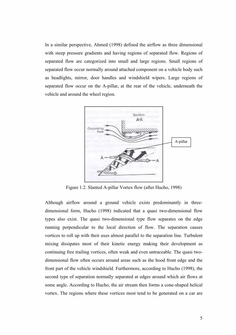
In a similar perspective, Ahmed (1998) defined the airflow as three dimensional
with steep pressure gradients and having regions of separated flow. Regions of
separated flow are categorized into small and large regions. Small regions of
separated flow occur normally around attached component on a vehicle body such
as headlights, mirror, door handles and windshield wipers. Large regions of
separated flow occur on the A-pillar, at the rear of the vehicle, underneath the
vehicle and around the wheel region.
A-pillar
Figure 1.2. Slanted A-pillar Vortex flow (after Hucho, 1998)
Although airflow around a ground vehicle exists predominantly in three-
dimensional form, Hucho (1998) indicated that a quasi two-dimensional flow
types also exist. The quasi two-dimensional type flow separates on the edge
running perpendicular to the local direction of flow. The separation causes
vortices to roll up with their axes almost parallel to the separation line. Turbulent
mixing dissipates most of their kinetic energy making their development as
continuing free trailing vortices, often weak and even untraceable. The quasi two-
dimensional flow often occurs around areas such as the hood front edge and the
front part of the vehicle windshield. Furthermore, according to Hucho (1998), the
second type of separation normally separated at edges around which air flows at
some angle. According to Hucho, the air stream then forms a cone-shaped helical
vortex. The regions where these vortices most tend to be generated on a car are
5

behind the A and C pillars (Refer Figures 1.2 and 1.1). The axes of these vortices
run essentially in the stream wise direction. The three dimensional vortices are
very rich in kinetic energy and this containment in kinetic energy are determined
by the ground vehicle geometrical conditions, mainly by the inclination of the A
r C pillar angle at which they separate.
.3 Overview on Sound and Noise
hich will in turn send electrical
pulses along the auditory nerve to the brain.
ness2. The sound pressure level
cale is measure in decibel (dB) and is defined as:
o
1
According to Barnard (1996), noise is the effect of pressure wave fluctuations
transmitted to the human ear at the speed of sound. Sound waves reaches the
human ear will travel through the ear passage to the eardrum causing it to vibrate.
The three bones situated in middle ear region will then transmit and amplify the
vibrations from the eardrum to the oval window in the inner ear region. Fluid in
the inner ear then stimulates nerve endings, w
im
Sound pressure waves that are continuously received by the eardrum over time are
random in nature (Figure 1.3). According to Buley (1997), the human ear can
withstand over a large range of sound pressure variation that are being transmitted
to it. The weakest sound pressure variations detectable by the human ear are of 20
μPa and because of this, a logarithmic scale was devised in order to provide a
good subjective for the human ear to perceive loud
s
2
0
log10 ⎟⎟⎠
⎞⎜⎜⎝
⎛=
ppSPL (1.1)
he sound pressure level with po as the
ference sound pressure level at 20 μPa.
P is defined as the root mean square of t
re
2 According to Buley (1997), loudness is how the human ear perceive the intensity or energy of the sound pressure variation.
6

Figure 1.3. High Pressure Zone in a Vortex Flow behind a Backward-Facing Step
(after Hucho, 1998 and adapted by Alam, 2000)
In the field of acoustics, the number of oscillation cycle it takes for sound pressure
wave to complete in one second (or the number of periodic wave cycle completed
in a given time period) is defined as Frequency, and is measured in Hertz (unit of
s-1).
TFrequency 1= (1.2)
In order to identify prominent frequency range in a random sound pressure wave
distribution, Fourier analysis is conducted where a finite set of random sound
pressure signal from a source is feed through a spectrum analyzer via a receiver
(microphone), which then performs a Fast Fourier Transform (FFT). In a FFT, the
random sound pressure signal is decomposed into several frequency bands,
determined by band pass filters used in the spectrum analyzer. The end results are
presented in a power spectra curve, often in a graph plot of SPL versus frequency,
Callister et al. (1998).
According to Buley (1997), the human hearing ranges from 20 Hz to 20 kHz in
frequency. The human ear is unique in such that its response to different types of
frequencies are not equally sensitive. It is most sensitive at frequencies between
7

the ranges of 1 to 5 kHz and is not particularly sensitive frequencies that are either
very high or low.
Fletcher and Munson (1933) investigated human hearing variation with various
frequency and found that the ears response to sound frequency differently at
different perceived levels of loudness. From their findings, they then plotted a set
of 'equal loudness' contours that can provide a way to measure loudness across a
broad frequency range (Refer Figure 1.4).
Figure 1.4. Fletcher Munsen Curve (from Buley, 1997)
The loudness contours are measured in phon. For an example, at a 40-phon
loudness level, a 63 Hz frequency must have a sound pressure level of around 58
dB to be as equally loud as a 1 kHz frequency with a sound pressure level of only
40 dB.
Because the human ear does not respond well against certain frequencies, a sound
weighting scale was developed in accordance to how the human ear perceives
loudness at different frequencies. There are four weighting scales (A, B, C and D)
currently accepted and used worldwide for sound measurements. The ‘A’
weighting scale represents equal loudness at the 40-phon loudness level, Norsonic
8

(www.norsonic.com). It is normally used to measure sound in the 20 - 55 dB
range, Harris (www.termpro.com). The ‘A’ weighting scale response similarly to
the human ear in that it discriminates low frequencies and response effectively
towards frequency in the 1 to 5 kHz range. The ‘B’ weighting scale represents
equal loudness level at 70-phon and used to measure sound in the 55 to 85 dB
range, Norsonic (www.norsonic.com), Harris (www.termpro.com). The ‘C’
weighting scale represents equal loudness level at 100-phons and used to measure
sound above the 85 dB range, Norsonic (www.norsonic.com), Harris,
(www.termpro.com). The ‘C’ weighting scale are normally used to detect sound
pressure levels in the low frequency range. According to Alam (2000), the ‘D’
weighting scale is originally developed to evaluate aircraft noise measurements.
Table 1.1: Weighting Scale for Perceived Loudness (adapted from Buley, 1997)
Frequency Hz 32 63 125 250 500 1000 2000 4000 8000
Curve A dB -39 -26 -16 -9 -3 0 +1 +1 -1
Curve B dB -17 -9 -4 -1 0 0 0 -1 -3
Curve C dB -3 -1 0 0 0 0 0 -1 -3
From Table 1.1, it can be seen that at 1 kHz (the lower threshold of human
hearing sensitivity), there will be no adjustment needed for the A-weighting scale.
Any sound pressure level located in a lower or higher frequency band will then be
adjusted accordingly based on the perceived loudness of the human ear.
Based on the definition of noise provided earlier in this section, it can be said in
general that noise is sound that is perceived as annoying. However, this remains a
subjective matter since sound that is annoying to a person might not be annoying
to another. According to Buley (1997), health, safety and environment are the
three criteria that are used to assess the acceptability of noise. The Victorian
Health and safety Regulations impose a limit to noise exposure for a maximum of
85 dB (A) in an 8 hours a day working environment. Any exposure higher than
the limit imposed can cause hearing impairment to the employee. Several different
of noise assessment scale are used to assess noise. The noise rating curve and the
noise dose calculation chart are some of the example of the noise scaling system
9
used. For motor vehicle in Australia, existing design rules (ADR28) allow a
maximum limit of 90 dB (A) for a passenger car that remains stationary, with a
maximum limit of 77 dB (A) while the car is in motion. In Europe, the rule is
slightly stricter with 74 dB (A) as the maximum allowable noise limit for a
passenger car to operate on the road.
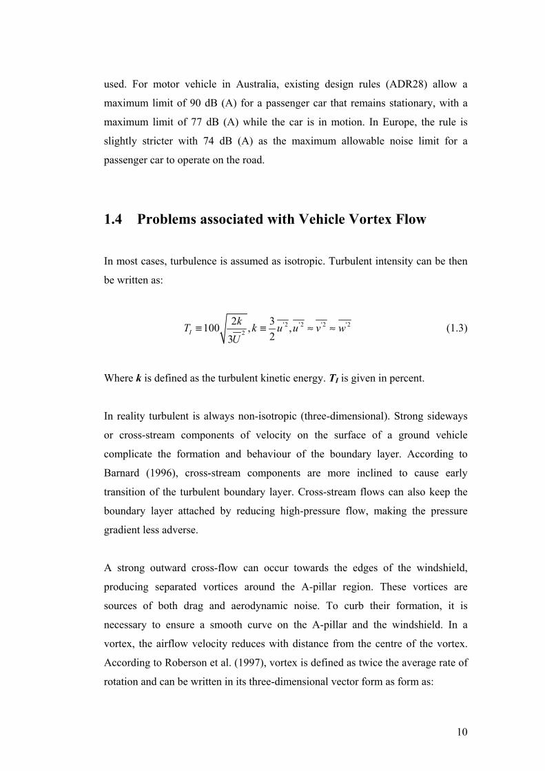
1.4 Problems associated with Vehicle Vortex Flow
In most cases, turbulence is assumed as isotropic. Turbulent intensity can be then
be written as:
'2 '2 '2 '22
2 3100 , ,23
IkT k u u v
U≡ ≡ ≈ w≈ (1.3)
Where k is defined as the turbulent kinetic energy. TI is given in percent.
In reality turbulent is always non-isotropic (three-dimensional). Strong sideways
or cross-stream components of velocity on the surface of a ground vehicle
complicate the formation and behaviour of the boundary layer. According to
Barnard (1996), cross-stream components are more inclined to cause early
transition of the turbulent boundary layer. Cross-stream flows can also keep the
boundary layer attached by reducing high-pressure flow, making the pressure
gradient less adverse.
A strong outward cross-flow can occur towards the edges of the windshield,
producing separated vortices around the A-pillar region. These vortices are
sources of both drag and aerodynamic noise. To curb their formation, it is
necessary to ensure a smooth curve on the A-pillar and the windshield. In a
vortex, the airflow velocity reduces with distance from the centre of the vortex.
According to Roberson et al. (1997), vortex is defined as twice the average rate of
rotation and can be written in its three-dimensional vector form as form as:
10

kyu
xvj
xw
zui
zv
yw
⎟⎟⎠
⎞⎜⎜⎝
⎛∂∂−
∂∂+⎟
⎠⎞
⎜⎝⎛
∂∂−
∂∂+⎟⎟
⎠
⎞⎜⎜⎝
⎛∂∂−
∂∂=Ω (1.4)
Furthermore, according to Roberson and Crowe (1997), vortex can be identified
either as forced vortex or a potential vortex. In a forced vortex, the airflow
velocity increases linearly from the vortex centre. In a free vortex, the airflow
velocity decreases exponentially from the vortex centre (Refer equation 1.5).
Forced vortex occurs due to the presence of viscous slipping between adjacent
layers of fluid molecules.
rVkrV
Free
Forced
/1∝=
(1.5)
Real life vortex flow has a combination of both free and forced vortex structure
(Refer Figure 1.5). The airflow velocity is high in the centre of the vortex,
resulting in the formation of region of high negative pressure.
Figure 1.5. Forced and Free Vortex Velocity Distribution (from Roberson and
Crowe, 1997)
Both quasi two-dimensional and three-dimensional vortices can lead to a
development of skin friction and pressure drag on the ground vehicle. The total
11

drag production from the development of skin friction and pressure drag will
result in the loss of performance and an increase in the vehicle’s fuel
consumption. The main contributor of vehicle drag is the rear portion of the
vehicle, which is not the focus of this study.
Apart from producing drag, the three-dimensional vortices are more detrimental in
a sense that they also impose effects on the vehicles occupants. The vortices on
the A-pillars impart stress on the front side windows of the ground vehicle. This
will lead to the development of aerodynamic noise (also known as Aeroacoustics).
Aerodynamic noise is then transferred to the passenger cabin that can be annoying
and can cause both fatigue and discomfort to the occupants in the car after a long
trip. Furthermore, interior vehicle noise makes it hard for vehicle occupants to
communicate with each another and to listen to the radio or compact disc player.
However, aerodynamic noise is a problem to the occupants at vehicle cruising
speed of higher than 100 km/h (60 mph). At lower speed, the dominant noise
sources are from the engine and tyres, George (1990), Callister et al. (1998).
According to Callister et al. (1998), the vehicle A-pillar area is a major wind noise
contributor and efforts has to be taken in designing the A-pillar to reduce
aerodynamic noise. Other vehicle body parts that are responsible for aerodynamic
noise are the junction between the bonnet and windshield, the roof racks, the
vehicle C-pillar, and gaps between the doors. In addition, add on parts on the
vehicle, such as the radio antenna, windshield wipers and external rear view
mirrors are also contributors to aerodynamic noise. George (1990) defined these
add on parts as parasitic noise source. The A-pillar is relatively close to the front
seat occupant’s ear, so noise in this area is noticed readily. The flow around most
A-pillar is separated, causes intense turbulent vortex flow to form on the side
window behind the A-pillar. Noise generated by the A-pillar is of broadband type
in nature and in the low frequency region, caused by the large scale turbulent
eddies from the A-pillar vortex separation, Haruna et al. (1990, 1992), George et
al. (1997), AVL (www.avl.com), (2003). There are several reasons why the A-
pillar contributes highly towards interior noise generation. One reason is that a
few vehicle body components are joined together around the A-pillar area
12

(windshield, the door, the outside rear view mirror and the front vehicle quarter
panel). Problems that usually suffice from this are normally due to poor sealing
and fitting problems. Callister (1998) explained that an auxiliary seal is definitely
needed to seal the A-pillar gap on doors with fully framed windows. This will
stop the pressure fluctuations to creep inside the vehicle transferring unwanted
noise. Another reason for noise generation around the A-pillar area is due to the
fact that flow around the A-pillar possesses relatively high velocities. Any
exposed cavity or protuberances will cause a high level of wind noise. Callister
(1998) quoted Watanabe et al. (1978) in saying that the flow around the A-pillar is
normally at around 60% higher than nominal free stream velocity. Considering
that wind noise starts to impose problem at speed above 100 km/h, close to the
surface of the car and around the A-pillar, the air velocity will be around 160
km/h. This increase in local velocity will result in a low local pressure level,
especially at the core of the vortex, Barnard (1996). The resulting dipole type,
high sound pressure level in the low frequency region (100 to 500 Hz) is
proportional to the sixth power of velocity, Haruna (1992). In accordance to the
sixth power proportionality rule, George (1990) indicated that local area of
separation with coefficient of pressure (Cp) of –1.0 will result in a 9dB sound
pressure level increase while a Cp value of -2.0 will result in a sound pressure
level increase of 14dB. In addition, any wind noise located around the A-pillar
region is around 17 dB louder than a source exposed to the free-stream velocity,
Callister et al. (1998).
1.5 Vehicle Noise
According to Ahmed (1998), there are two types of noises that are of a concern to
vehicle designers. The noises are drive-by noise, which affects people outside the
vehicle and interior noise, which affects the driver and passenger. George et al.
(1997) described that the vehicle noise heard by people outside the vehicle is
called exterior vehicle noise and the vehicle noise heard by the automobile
occupants as interior vehicle noise.
13
Exterior and interior vehicle noise is transferred to the surroundings either through
the vehicle structure (structure borne) or via external airflow around the vehicle
(air borne). Structure borne noise originates through vibration of vehicle structure.
An example of structure borne noise is noise that originates from vehicle tire
dynamic interactions with the road surface. Another example of structure borne
noise is vibration effects from vehicle mechanical components such as vehicle
powertrain systems (engine and transmission). Air borne noise originates through
forces generated from air that flows around and through the vehicle. Examples of
air borne noise are noise generated from the vehicle ventilation and exhaust
system, engine air intake, A-pillar and side mirror.
Exterior noise originates mainly from the powertrain systems and tyres. However,
According to George (1995), extensive efforts have been put forward over the
years to minimise engine and tyre noise. Work has been done towards reducing
engine noise such as adding sound absorbent materials material surrounding the
engine compartment and developing larger capacity mufflers to reduce exhaust
noise. Through out the years, manufacturers have succeeded in reducing tyre
noise. According to Affenzeller et al. (2003), for modern day tyres, emphasis have
been put on modifying tyre tread, making them more randomised to avoid high
tonal noise and making the grooves on tyre tread more ventilated for better
pressure distribution. This is attributed to the fact that modern tyres are wide and
offers better grip on the road surface, thus making it much noisier. For vehicle
speed below 100mph (160 km/h), reduction on tyre noise has been lower than
engine and drive train noise, George (1990).
Interior vehicle noise originates from various sources from the vehicle. Vehicle
ventilation system, engine and tires are contributor to vehicle interior noise.
Engine and tyre noise contributes to interior noise predominantly at low vehicle
speed. Interaction between air and the external vehicle body parts also contributes
to interior noise. This phenomenon is classified as ‘aerodynamically induced
noise’ or ‘aerodynamic noise’ and is the domain of vehicle aeroacoustics study.
According to George (1990, 1995) aerodynamic noise starts to become dominant
when vehicle is traveling at high speed, at around 70 mph or greater. Furthermore,
14

George (1995) stated that aerodynamic noise is dominant in frequency region of
between 500 to 12 kHz. At present, aerodynamic noise is seen mainly as problem
of the internal environment rather than the external environment of the vehicle.
According to Callister et al. (1998), interior vehicle noise is annoying because it
makes it harder for occupants to communicate with each another. Furthermore, it
makes it hard to listen to the radio or compact disc player. Moreover, interior
noise can cause fatigue to the driver on long trips. According to George (1990)
interior noise is causing significant comfort problems at cruising speed of around
60 mph (96 km/h) and above. Interior noise around this vehicle speed ranges
between 70 to 80 dB, making long trips inside a vehicle discomforting and tiring
to occupants. Barnard (1996) reviewed a study on a small car at 150 km/h and
found that the engine contributes to 82.5 dB of interior vehicle noise. Tires and
aerodynamic noise contributes to 78.0 dB and 78.5 dB respectively. Barnard
(1996) quoted Buchheim et al. (1968), which conducted a study on 15 different
vehicles and found interior noise level at vehicle speed of 113 km/h ranges
between 62 to 78 dB (A) and rising to 72 to 87 dB (A) at 180 km/h, which is
slightly higher than the industrial workplace limitations of 85 dB (A).
In addition, a vehicle with low aerodynamic drag does not necessarily will have
low levels of aerodynamic noise. Buchheim et al., surveyed fifteen production
cars in 1982 and found that aerodynamic drag and aerodynamic noise are
independent of each another. Aerodynamic drag depends predominantly on the
exterior airflow over the rear of the car where flow separation is occurring while
aerodynamically induced vehicle noise depends mainly on exterior airflow around
the A-pillar and windshield where small openings or imperfectly seal of the doors
and windows that may generate strong unsteady pressure fluctuations that
resulting in vehicle interior noise generation, Callister et al. (1998). George et al.
(1997) added that aerodynamic drag depends on the transient mean pressure
distribution on the vehicle surface. However, vehicle aerodynamic noise depends
on the strength of the surface pressure fluctuations relative to the mean value.
15
1.6 Mechanism of Aerodynamic Noise Generation
Callister et al. (1998) described that for aerodynamic noise, the generation
mechanism must include a ‘source’, ‘path’ and ‘receiver’. The ‘source’ is
described as the area where energy is converted into acoustic energy. The acoustic
energy then radiates from the source location and is transmitted through different
mediums i.e. liquid or through solids. George et al. (1997) described the interior
vehicle aerodynamic noise ‘source’ as the fluctuating pressure caused by the
turbulent flow around the car, flow over gaps and protrusions and leaks. The
‘path’ is described as the route along which the acoustic energy is transmitted on
its way to the receiver. It can be either through clear travel passage through leaks
or cavity or through vibration of the vehicle body shell radiating acoustic energy
into the vehicle. The ‘receiver’ is the person or microphone that receives the
acoustic energy and converting it into sound pressure signals.
Identification of aerodynamics noise source can be done through the development
of idealized models. According to Callister et al. (1998), aerodynamic noise can
be classified into either monopole, dipole and quadrupole idealised model.
The monopole source effect originates from an unsteady introduction of volume
into the surrounding fluid. It is the most efficient sound generator at low mach
numbers. The most notable monopole source of noise for automobiles comes from
unsteady volumetric flow addition. If a fluctuating pressure on the vehicle exterior
surface causes an unsteady volumetric flow addition to the interior of the car
through a leak path, then a strong secondary monopole sound source will result.
Callister et al. (1998) quoted Norton (1989), in stating that a good example of
monopole sound is to come from the un-muffled vehicles engine intake and
exhaust pipe.
Dipole source effect is the next most efficient generator of sound at low Mach
numbers. Dipole effect is the caused by unsteady forces to the fluid resulting in
unsteady pressures to act upon rigid surfaces on a vehicle. Noise from a separated
turbulent flow impinging upon a surface is an example of dipole noise.
16
Automobiles typically have numerous separated flow regions with the A-pillar
being arguably the most popular with its aerodynamic noise generation
capabilities.
The least efficient sound source at low Mach numbers is called the quadrupole
source effect. Quadrupole source effect is caused by internal stresses and
turbulence within the flow. It is best described as two fluid elements colliding
with each other, as might happen in a turbulent shear layer. Jet noise is an
example of quadrupole source effect Goldstein (1976). Quadrupole source effect
can usually be ignored in automotive flows since they are comparatively very
weak when compared to monopole or dipole type source effect.
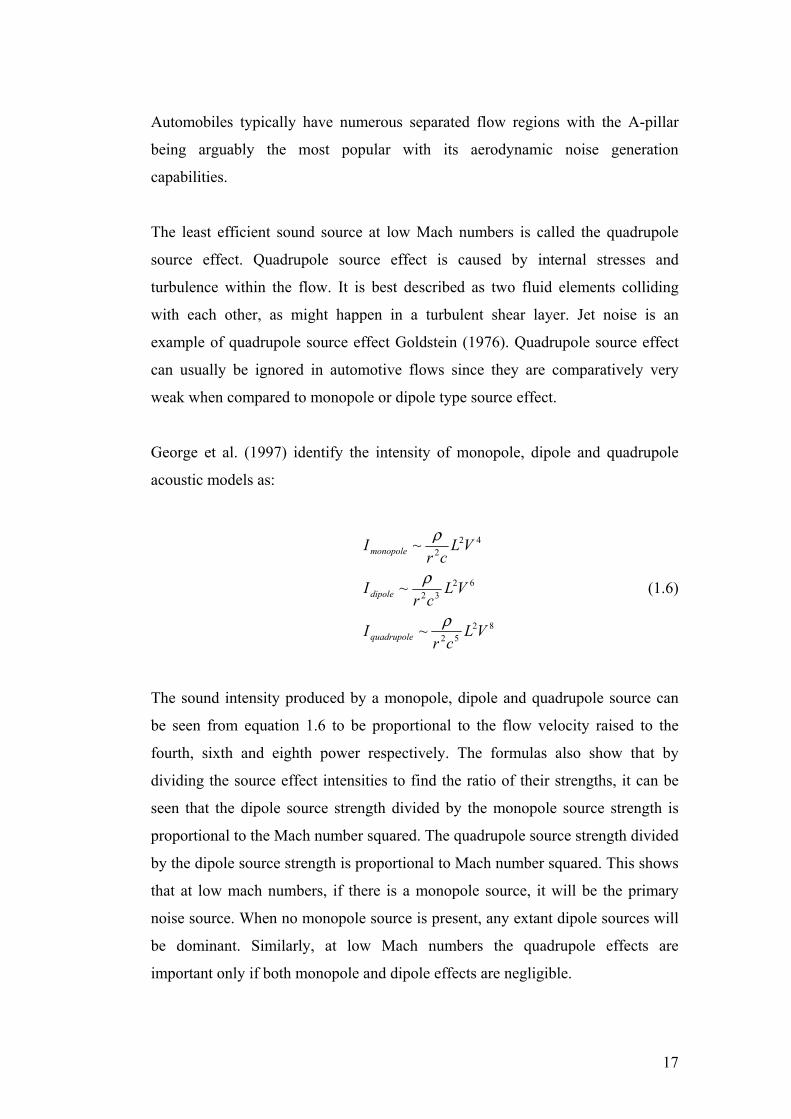
George et al. (1997) identify the intensity of monopole, dipole and quadrupole
acoustic models as:
8252
6232
422
~
~
~
VLcr
I
VLcr
I
VLcr
I
quadrupole
dipole
monopole
ρ
ρ
ρ
(1.6)
The sound intensity produced by a monopole, dipole and quadrupole source can
be seen from equation 1.6 to be proportional to the flow velocity raised to the
fourth, sixth and eighth power respectively. The formulas also show that by
dividing the source effect intensities to find the ratio of their strengths, it can be
seen that the dipole source strength divided by the monopole source strength is
proportional to the Mach number squared. The quadrupole source strength divided
by the dipole source strength is proportional to Mach number squared. This shows
that at low mach numbers, if there is a monopole source, it will be the primary
noise source. When no monopole source is present, any extant dipole sources will
be dominant. Similarly, at low Mach numbers the quadrupole effects are
important only if both monopole and dipole effects are negligible.
17

Automobile aerodynamic noise is typically a mixture of monopole and dipole
sources. According to George (1990), automobile aerodynamic noise is
proportional to the sixth power of the flow velocity. This was confirmed by a
study conducted by Haruna et al. (1992). Therefore this explains the reason
vehicle aerodynamic noise dominates tire noise and engines noise at high vehicle
speeds.
Earlier in this sub-section, the concept of source, path and receiver was mentioned
for the complete transmission of aerodynamic noise to take place. However, this is
a generalized concept for aerodynamic noise generation. In reality, the
aerodynamic noise can be transmitted either through a leak, cavity or can be
generated through airflow turbulence interaction with the vehicle body.
Aerodynamic noise generated through a leak is called a leak noise (or sometimes
called aspiration noise) and it can occur in two ways. According to Callister et al.
(1998), leak noise could be caused by movement of airflow through an area of
small leaks, which connects the exterior, and the interior of the vehicle. George
(1990) further added that leak noise propagation could also be transmitted through
panels, windows and seal, due to the fact that their transmission losses are less
than 100%. Both mechanism of leak noise can be seen in Figure 1.6.
Figure 1.6. Two method of Leak Noise Transmission (From Callister et al., 1998)
18

Callister et al. (1998) further described that airflow movement at a rather high
velocity causes leak noise, transmitted from a high-pressure zone to a lower
pressure zone. George et al. (1997) further mentions that it is not unusual for leak
noise to increase interior noise by as much as 10 dB. Leaks are normally present
on vehicle door seals, movable glass seals and the fixed glass seals. Furthermore,
according to George et al. (1997, leak noise can be transmitted by either through
steady or unsteady pressure from the vehicle exterior. If the leak comes into
contact with the external surface of the vehicle that is experiencing turbulence
separation and generating pressure fluctuation, then the mass flow entering the
leak will be unsteady, generating monopole sound inside the car. The tonal and
fluctuating nature of monopole sound will result in a high frequency noise, which
is noticeable and annoying, George et al. (1997). This is illustrated in the top part
of Figure 1.6 where a defective seal can generate monopole sound due to
fluctuating external pressure at location one. This will affect the mass flow
through to location two. Secondly, if the leak connects to a steady pressure source
generate steady flow of air through the leak opening, flow will only starts to
separate in a turbulent manner after the location two areas, thus generating local
fluctuating pressures. This gives rise to dipole type sound, which is transmitted
into the vehicle.
The second mechanism of leak noise can be seen in the bottom part of Figure 1.6,
which shows how leak noise can be transmitted through a seal, even when there
are no leaks. According to George et al. (1997), the external pressure at point one
can move the seal forward and backwards slightly and generate sound. The seal
will absorb some of the noise. According to George et al. (1997), by doubling the
seal mass, sound pressure level will increase only by 3 dB in attenuation. Using
multiple seals however, can provide up to 5 dB in interior noise reduction in some
cases. George et al. (1997) referred to the work by Danforth et al. (1996) for a
recent experimental study on effect on single and double seal on noise flow. Other
references on leak noise mechanism can be seen from Callister et al. (1998), who
referenced the work of Jung et al. (1995), describing a recent study by the authors
on the influence of leaks on the interior wind noise level.
19

The second method of aerodynamic noise transmission is through a cavity, and
can be described as cavity noise. As per leak noise, cavity type noise is also often
located in region of high velocity flow, such as the exposed gaps around the A-
pillar area or around the outside rearview mirror, Callister et al. (1998). George et
al. (1997) divides cavity noise into two categories namely large (i.e. open
windows and sunroofs) cavities and small cavities (i.e. door gaps) respectively.
George (1990) also divided cavity noise into two types, broadband type noise and
tonal type noise. Similar to leak noise, cavity noise is of monopole and dipole type
origin.
George (1990) and Callister et al. (1998) described broadband noise as noise
caused by turbulent boundary layer flowing across the cavity creating trailing
edge noise as it passes over the cavity. A turbulent free shear layer then develops
as the flow leaves the cavity. It then impinges itself on the rear of the cavity
generating leading edge noise, resulting in cavity noise displaying broadband
frequency characteristics (Refer Figure 1.7).
Figure 1.7. Mechanism of Cavity Noise Transmission (From Callister et al., 1998)
George (1990) and Callister et al. (1998) further described that besides the
broadband cavity noise, a tonal type cavity noise can also be generated. Tonal
type cavity noise generation involves a feedback and resonance mechanism.
Similar to broadband type cavity noise, the tonal type cavity noise involves
disturbance shedding from the front edge of the cavity. This disturbance impinges
on the rear edge of the cavity generating acoustic wave tones that propagates in all
directions. When the acoustic wave reaches back to the front edge of the cavity, it
20

then triggers another shedding of disturbance, giving it a feedback and resonance
type phenomenon. According to George (1995), this feedback can be acoustic or
convective and it can involve ordinary acoustic modes of a cavity or Helmholtz
type resonance (Refer Figure 1.7).
George et al. (1997) further adds that large cavity noise generates mostly low
throbbing frequency noise, which can be both annoying and fatiguing. Small
cavity noise on the other hand is most likely to generate high frequency noise.
High frequency noise is much easy to absorb with carpeting and upholstery. Low
frequency noise however, is more difficult to absorb. Helmholtz type resonator
damping, damped panels or active damping will have to be used in order to
minimize it (George, 1990). Callister et al. (1998) referred the work Rockwell et
al. (1978) on cavity noise for further reading.
The third and final method of aerodynamic noise mechanism is due to turbulence
airflow interaction with the vehicle body. This can be described as wind rush
noise, Callister et al. (1998). It is generated by fluctuating pressures on the
exterior of the vehicle caused by the fluctuating, unsteady turbulent airflow over
the surface (Refer Figure 1.8). Wind rush noise will always be present over the
vehicle surface even though the vehicle surfaces were perfectly rigid and leak-free
and the flow are attached throughout the vehicle surface due to the turbulent
nature of boundary layer on the surface of the vehicle. However, if the flow is
separated, the noise generated will be intensified by a factor of approximately ten,
Callister et al. (1998). Wind rush noise will initiate dipole effect source type
effect, radiating outward in all directions and since the vehicle is not perfectly
rigid, the fluctuating pressure impinging on the vehicle windows and body panels
will result in vibration, radiating noise into the vehicle interior. In addition, wind
rush noise is broadband in nature but is less annoying than tonal noise.
21

Figure 1.8. Wind Rush Noise Transmission around Vehicle (From Callister et al.,
1998)
1.7 Ways of Reducing A-pillar Aerodynamic Noise
In vehicle design, the aim is to reduce interior noise through altering vehicle body
design, without adding extra component to the vehicle, as this will add additional
cost to the overall vehicle production. In order to reduce aerodynamic noise
generation at the A-pillar region, the size and intensity of the A-pillar vortex must
be reduced. In theory, Haruna et al. (1990) proposed that aerodynamic noise is
dependent on properties such as the surface fluctuating pressure, the frequency
and the correlation area. Therefore, minimisation of aerodynamic noise could be
done by suppressing the surface fluctuating pressure and frequency, and by
reducing the correlation area. According to George (1990), high frequency noise
that propagates into the vehicle can easily be absorbed by carpet and upholstery.
Low frequency noise can be reduced through the use of Helmholtz resonator
damping, damped panels or active damping.
In a physical sense, one way to reduce aerodynamic noise is to design vehicles
with a small inclination angle between the windshield and bonnet, Scibor-Rylski
(1984). Alam (2000) mentioned in his work that the average windshield
inclination angle for a passenger car is around 60°. However, it was mentioned by
Hucho (1998) that small windshield inclination angle with the bonnet will not
further reduce drag and it also impose visibility and temperature problems to the
22
vehicle occupants. Another way of reducing A-pillar vortex size and intensity was
recommended by Callister et al. (1998) in that the radius of the A-pillar has to be
large to further minimise the airflow velocity and turbulence intensity. This
proved to be true. Experiments conducted by Alam (2000) on simplified vehicle
models at various yaw angles3 have showed that by increasing the A-pillar
windshield radius, a decrease in ‘in cabin noise’ was obtained particularly in the
leeward side of the vehicle. It was also recommended by Callister et al. (1998)
that the A-pillar region to be designed without exposed rain gutter. Exposed rain
gutters will usually cause wind noise as it cause flow to separate at the edge of the
A-pillar. Again this proved to be true based on experiments carried by Alam
(2000), which showed that by adding a rain gutter on the A-pillar, an increase in
fluctuating pressure was obtained behind the A-pillar region. A study by Piatek et
al. (1989) has shown a simple modification carried out on the vehicle A-pillar to
redirect rainwater without having to design an exposed rain gutter.
According to Callister et al. (1998), outside rear view mirrors also exists as a bluff
body that contributes to the disturbance of the flow pattern around the A-pillar
area. Coupled together with the A-pillar vortex, airflow separation behind the A-
pillar can result in high wind noise levels. A study made by Hamel et al. (1996),
have showed that the rear view mirror contributes to the increase of wind noise up
to 20 dB (130 dB with mirror and 110 dB without mirror) at region downstream
close to the side mirror, dominating in the frequency spectrum range of lower than
1 kHz. Lokhande et al. (2003) conducted an LES simulation of a generic side
view mirror and also managed to obtain a sound pressure level peak of around 130
dB behind the mirror region. In addition, Fukushima et al. (1995) conducted a
study on aerodynamic noise from a side mirror and found out that pressure
fluctuation level generated behind the rear view mirror are around 90 to 100 dB.
Callister et al. (1998) recommended that the external rear view mirror to be
moved as far rearward as possible in order to minimise wind noise. This moves
the mirror out of the maximum flow speed area. However, careful placement must
be done so that the field of view of the driver is not restricted. In addition to that,
3 To simulate the effect of crosswind, vehicle or scaled model is rotated to various angle in the wind tunnel. This varying angle of rotation is called the yaw angle.
23

the exterior overall shape of the mirror must be carefully designed to minimise
induced wind noise. Normally aerodynamicists will design the rear view mirror
first aiming in achieving low drag and only secondly to minimise wind noise,
George (1997). Mirrors with a rounded housing are generally preferred with holes
and gaps in the mirror housing to be eliminated. This is to minimise trailing edge
noise generated by flow separation past sharp edges along the rear view mirror,
Callister et al (1998), George et al. (1997).
1.8 Vehicle Aerodynamics and Aeroacoustics:
Numerical and Computational Evaluation Methods
Numerical evaluation methods involving vehicle aerodynamics and aeroacoutics
can be done either analytically or by using Computational Fluid Dynamics (CFD).
Analytical methods in solving airflow behaviour realistically can be done on
simple generic type flow problems in either two-dimensional or three-dimensional
form. As airflow behaviour gets more complex when subjected to flow around
complex geometrical domain or bluff bodies, (with the presence of turbulence or
compressibility effect), solving airflow properties cannot be done analytically.
This is because in order to obtain its complete turbulent and aerodynamic noise
source properties, full unsteady Navier-Stokes (taking into account inertia,
viscous and pressure forces) together with the continuity equation (mass
conservation) need to be solved.
However obtaining a direct numerical solutions of Navier-Stokes equations are
still not yet possible even for modern day computers. The main reason being that
gird points needed for a typical CFD model to be solved are Re 9/4. For a typical
flow with Reynolds number of 106, it will take the computer to generate and solve
equations for 3.16x10¹³ gird points. This is far beyond the reach of even the most
state of the art supercomputers available in the world today. In order to come up
with a comparable solution, steady or time averaged Navier-Stokes equation is
used (called Reynolds Average Navier-Stokes equation – RANS) together with
turbulence model, developed to take into closure problems involving Reynolds
24
stresses resulting from the time averaging process. Solving for RANS, continuity
and turbulence model equations can be done via Computational Fluid Dynamics
(CFD) simulations.
CFD approach for turbulence modeling was first intended for the aerospace
community in the 1960s and 1970s (Anderson, 1995). In the early development
stage of CFD for automotive applications, codes were expected to provide actual
quantitative data that is similar to measured wind tunnel data. Knowing that this is
not yet possible, present use of CFD in automotive are used to provide
information about flow characteristics and phenomena, which dictates
aerodynamic performance. However, the ultimate goal in CFD is to obtain model
as flow as actual as possible and current and future research on CFD is ongoing in
order to achieve that goal. Furthermore, current applications of CFD in the
automotive industry are determined by economics viability. To be economically
viable, the codes should be able to simulate the correct physics of the flow and at
the same time achieve computational turnaround time that is the same or less than
that of a wind tunnel test cycle time. Ahmed (1998) has showed that for a typical
vehicle, current testing time taken in a wind tunnel in order to achieve desired
level of Cd reduction has increased. This will be an expensive exercise for
automobile manufacturers. With the reduction on computational cost,
aerodynamic simulation by using CFD, being run at a faster turnaround time will
only be at a fraction of the cost.
However, this will only put more demand on the current performance of
computers speed and memory. These are due to several factors:
• An increase sophistication of flow physics modelled.
• An increase in modelled geometries complexities.
• An increasing number of multidisciplinary approaches of flow simulation.
These increases in computational demands are intended in achieving the ultimate
goal ‘fluid flow realism’ in CFD simulation as mentioned earlier. A much more
complex three-dimensional vehicle geometries are now being used in automotive
25

CFD simulation coupled with high grid density to achieve better flow resolution.
Usually this also leads to a more accurate and realistic flow simulation. In an
unsteady three-dimensional flow, a doubling of grid density (to double the
accuracy) results in a (with three space coordinates and a time dimension) sixteen-
fold increase in computation effort. In addition, better CFD post processing flow
visualisation effect such as colour-coded pressure distributions over the entire
body surface and observation of particle traces in real time animation also puts
extra demands on computer speed and memory.
From the CFD results obtained through RANS simulations, aeroacoustics
properties of the flow can be extracted and analyzed. This branch of CFD
technique is called Computational Aeroacoustics Analysis (CAA). In CAA the
surface fluctuating flow data obtained from either steady state or time dependent
CFD simulation are used as source terms for CAA simulation. CAA simulation
technique can be categorized into three, which are the Lighthill Acoustic Analogy
Method, Kirchoff Method and Perturbation Method. Majority of study on CAA
incorporate the Lighthill Acoustic Analogy to evaluate for aerodynamic noise
propagation. The Lighthill Acoustic Analogy was made famous by the late
Professor Sir James Lighthill where in 1951 and 1954 introduced papers
proposing a theory on noise generation in free stream flow. Efforts were made by
Curle (1955, Ffowcs-Williams and Hawkings (1969) to extend Lighthill’s work to
include modeling of aerodynamic noise propagation around a solid body.
Computational Aeroacoustics Analysis is still new and is open to a lot of
discussion and ideas. According to Ogawa et al. (1999) in a review on
aerodynamic noise prediction using CFD, the accuracy of aerodynamic noise
prediction is dependent on the computational accuracy in solving transient flow.
However, similar to CFD, more work needs to be done with CAA especially on
flow around the A-pillar region in order to evaluate its performance under various
geometrical and flow environment. CAA based on the CFD results is limited to
external near-field noise radiated close to the vehicle surface. Recent
recommendations on how to better predict interior wind noise by combining data
from CFD and Statistical Energy Analysis (SEA) is given by Bremner et al.
26

(2003). By using SEA, researcher is able to predict structure borne noise that’s
being transmitted inside the car caused by external pressure fluctuations on the
vehicle surface. Other numerical analysis that uses SEA to predict structureborne
interior vehicle noise are given by De-Jong (1985), Yashiro et al. (1985),
Strumolo (1997), Yang et al. (1997), Iida (1999) and Manning (2003).
1.9 Literature Reviews on A-Pillar Aerodynamics and
Aeroacoustics Over the years, research studies concerning A-pillar aerodynamics have focused
mainly in understanding the mechanics of airflow behaviour when exposed to
various A-pillar and windshield configurations to help further reduce aerodynamic
noise. Research studies conducted are predominantly using experimental and
numerical method or a combination of both.
Stapleford et al. (1970) conducted experimental studies of aerodynamic noise
generation on a yawed rectangular shaped box at different yaw angles. External
aerodynamic noise was measured from various region of airflow. From their
studies, they found out that the aerodynamic noise generation was highest at the
region of vortex flow behind the A-pillar region. Aerodynamic noise generation
from vortex flow is around 120 dB, a 20 dB increase from the background tunnel
ambient noise. They also found out the highest sound pressure level was in the
region of low frequency, due to the large-scale turbulent structures at the area of
flow separation.
Fricke in (1968) and (1971) conducted a study on pressure fluctuations on
separated flow and concluded that the wall pressure fluctuations of subsonic
separated flow are an order of magnitude higher than those beneath a boundary
layer and that the source of wall pressure fluctuations is in the shear layer above
the re-circulating flow, close to the reattachment point. This was different to the
findings of Mohsen (1967) in which he discovered that maximum pressure
fluctuations occur near the reattachment region of the flow.
27

Laufer (1974) explained that noise formed from vortex generation is due
predominantly by vortex pairing or mixing. However, Hussain (1983, 1986)
argued that not all the vorticity component play a role in vortex noise generation,
with the breakdown of flow geometry i.e. separation, reattachment and vortex
breakdown also playing an important role.
Watanabe et al. (1978) experimented with a slanted angle A-pillar model that
showed a conical vortex structure generated behind the A-pillar region. High-
pressure region centered at the vortex core with intense pressure distribution being
strongest at the A-pillar base and area close to the A-pillar (Cp values is around -
2.0). The vortex flow grew weaker as it rotates further from the A-pillar base,
particularly around the roof region, next to the A-pillar (Cp values is around -0.7).
Buchheim et al. (1982) conducted experiments to investigate interior noise level
due to external aerodynamic noise generation on various components of a vehicle.
Around the A-pillar region, they obtained similar findings as per Stapleford et al.
(1974) in that aerodynamic noise generation was 20 dB higher from the
background noise. However, after modification of the A-pillar region, they
managed to reduce the aerodynamic noise generation around the A-pillar region to
the same level as the background noise. They concluded from their study that no
particular component of the car dominated in radiating interior noise. However,
interior noise level radiating from the A-pillar region is the highest at 60 dB (A)
and corresponds to region of low frequency (250 – 500 Hz).
Simpson (1987, 1989) explained that the effective pressure fluctuations of vortex
flow might be near the locus of maximum shear stress position of the separating
turbulent boundary layer. The large-scale motions produced in the vortex flow
separation do not contribute much to the turbulent shear stresses. It only changes
the mean flow-field to produce low frequency pressure fluctuation at low Mach
number.
28

Sadakata (1988) showed that at a critical A-pillar slant angle between 40° to 50°,
a sudden increase in sound pressure occurred. Sadakata and his colleagues
concluded that noise could be reduced considerably by combining the proper A-
pillar slant angle with curved windshield and smooth rounded A-pillar geometry.
Bearman et al. (1989) conducted several experimental tests with numerical type
validation of a passenger car and simplified scale models. The tests were carried
out to examine the effect of vortices generation in vehicle under wind yaw
condition while exposed to wind of 20m/s. A maximum yaw angle of 20° was
investigated with increment of 5°. It was observed that the effect of vortex
increases at higher yaw angle in the leeward region of the car with sudden
escalation after 10°. It was not mentioned however in the paper of the windshield
angle and radius used in the experiment. When surface pressure measurements
were taken on the surface of the A-pillar region (did not mention where exactly) at
0° yaw, it was found that minimum Cp was between –1.4 and –1.5. In addition it
was stated that the A-pillar region of flow were highly unsteady and the vortex
strength kept changing with time.
Haruna et al. (1990) experimented using a production car in a wind tunnel at 50
km/h and yaw angles of 0° and 10° respectively. From their study, they found out
that the separated region of the flow at 10° yaw is larger when compared to the
separation region at 0° yaw. They also found out that high sound pressure level
originated from side window surface fluctuations was sustained at a large area
when the car was yawed at 10°. High sound pressure level was observed at region
of low frequencies. The overall sound pressure level at when the vehicle is yawed
was at its highest at around 110 dB (A) and a difference of 10 dB (A) was
recorded when compared against vehicle at 0° yaw. Furthermore, they discovered
a primary and secondary vortex rotating opposite each other behind the A-pillar.
The vortex generated when the vehicle is at 10° yaw is greater in size (around 85-
mm in cross section) in comparison to the vehicle at 0° yaw angle (around 50-mm
in cross section). In addition, they also found that the separated region exhibit
rotational flow with the reattachment region having irrotational flows. However,
29

they failed to measure the size of vortex progressively throughout the span wise
length of the A-pillar.
Popat (1991) experimented on effects of windshield angle on A-pillar vortex.
Popat noted some Reynolds number sensitivities at different A-pillar slant angle
except for when the inclination angle is at 60°. Popat noted in his thesis three
stages of vortex formation at different A-pillar slant angle with only bubble
separation occurring below 20°, vortex-bubble separation occurring between 30°
to 40° and fully developed conical vortex occurring between 50° to 60° slant A-
pillar angle, which is what normally experienced on a normal production car.
Popat concluded that the critical angle at which peak mean and fluctuating
pressure values occurred at 40° inclination.
Haruna et al. (1992) developed a numerical model to estimate the distribution of
surface pressure fluctuation for aerodynamic noise prediction. They also validated
their model with experimental data. From the experimental data, they found out
that the highest contributor of aerodynamic noise is the A-pillar with overall
sound pressure level ranging between 110 to 130 dB, at different vehicle
velocities of 50, 100 and 140 km/h respectively. The aerodynamic noise generated
was dependent to the fourth power of vehicle velocity. From their experimental
results, they found out that high surface pressure fluctuation occur at the base of
the A-pillar region. Highest sound pressure level was predicted at 105.5 dB,
which correspond to a frequency of 500 Hz. From their model, they obtained
predicted aerodynamic noise distribution behind the A-pillar region at frequencies
range of between 100 – 500 Hz for vehicle velocity at 50 km/h, 200 – 1 kHz for
vehicle velocity at 100 and 300 – 1.5 kHz for vehicle velocity at 150 km/h. At 50
km/h, the highest sound pressure level was obtained at 107.7 dB at 150 Hz. At
100 km/h the highest sound pressure level was obtained at 120.6 dB at 300 Hz and
at 150 km/h the highest sound pressure level was obtained at 127.0 dB at 450 Hz.
In addition, noise intensities were also predicted. Highest recorded noise
intensities were 58.9, 76.8 and 83.9 dB, which corresponds to vehicle velocities of
50, 100 and 140 km/h respectively. From their model, the aerodynamic noise was
at fifth power to the vehicle velocity.
30
Haruna et al. (1992) developed a numerical model to analyze aerodynamic noise
on a delta wing (to mimic A-pillar flow) for incompressible flow. Numerical
investigation was conducted at six different velocities between 50 to 200 km/h.
The numerical model that was developed was divided into two parts. The first part
was developed using continuity and unsteady Navier-Stokes equation to solve for
flow properties on the delta wing. However, Haruna failed to mention the time
steps taken in the simulation. Results from the first part were then used to solve
for aerodynamic noise. Equations used for the outer region was developed from
the Lighthill - Curle’s for acoustic radiation from a solid body. Results of
fluctuating pressures against time were obtained. Results did not show good
agreement against empirical data although it showed similar trend. They also
obtained spectral analysis of the aerodynamic noise prediction. Spectral analysis
against measured results showed that the predicted results were under predicted
by about 20 dB. However, predicted results managed to capture the trend of
results obtained from measurements. The author concluded that the under
prediction might be caused by insufficient amount of grids generation. High sound
pressure level was obtained at frequency region of below 1 kHz. In addition,
results showed sound radiated from the delta wing to be of dipole sound strength,
which correspond to the power of sixth velocity, which is in agreement to the
Lighthill-Curle’s equation, (Curle, 1955).
Hanaoka et al. (1993) conducted a numerical simulation to determine A-pillar
aerodynamic noise behaviour at different windshield slant angle (30°, 45°, 52.5°,
60° and 75°s from horizontal axis) at 100 km/h using quasi DNS method (at time
steps of 10 mili-seconds with 0.6 second sampling case to correspond at Courant
number of 0.4) and Lighthill-Curle equation (to solve for noise). Results from the
simulation showed an increase in wind noise with windshield angle especially at
critical angle of above 50°. Results also showed that main aerodynamic is of
dipole sound source and originated from area of vortex separation and
reattachment together with turbulent shear interaction with the side window roof
area. Furthermore, pressure spectra results showed high wind noise at low
frequency range caused by large scale eddies. The highest peak of predicted
31
overall sound pressure level was obtained at 110 dB for the 75° vehicle model and
the lowest peak of predicted overall sound pressure level was obtained at 45 dB
for the 30° vehicle model. In addition, time averages surface pressure distribution
was also predicted. The highest Cp value obtained was at the center of the vortex,
which location shifted closer to the base of the A-pillar as the slant angle
increases. Highest recorded Cp value was –4.0 at 60° slant angle and the lowest
recorded was –1.6 at 30° slant angle. However, study failed to show any
comparison with empirical data and points of measurement for predicted overall
sound pressure level.
Nienaltowska (1993) experimented with flow behind the A-pillar at various
velocity and measured pressure and velocity fluctuations at points away and
perpendicularly from the side window. Nienaltowska found that turbulence
generation is independent of velocity and that it decreases with wall distance.
Turbulence generation is highest in the direction perpendicular to the flow (w-
component). In addition, Nienaltowska also explained that aerodynamic sound
production occurs when vortex lines are stretched or accelerated relative to the
acoustic medium.
Zhu et al. (1993, 1994) obtained from their numerical study using commercial
CFD software SCRYU with different A-pillar slant angle at different velocities
that the sound intensity level increases with vehicle speed. The numerical study
was time dependent conducted at time steps of 10 mili-seconds, which correspond
to courant number of 0.4. Furthermore, they found that the A-pillar aerodynamic
noise was generated through both vortex generation and breakdown process.
Moreover, high-pressure fluctuations seem to be occurring at the front side
window and roof side junction with pressure fluctuations at the roof junction
much more higher compared to the ones generated behind the A-pillar and
occurring higher at higher A-pillar slant angles. Results obtained were similar to
the study conducted by Hanaoka (1993). No validations of predicted numerical
results were made with empirical data.
32

Dobrzynski et al. (1994) conducted experiment on the A-pillar region at different
yaw angles. He found that huge surface pressure level reduction can be achieved
when using smooth A-pillar contour with large radius and flushed side windows
compared to using large radius A-pillar with recessed side window.
Hamel et al. (1996) include side mirrors on his A-pillar experiment with various
height and vehicle velocities. The addition of side mirror in the experiment
increases fluctuating pressure level as much as 20 dB (from 110 dB to 130 dB) at
lower frequency downstream close to the side mirror (below 1kHz). No
significant increase in sound pressure level close to the A-pillar as a result of side
mirror addition. However, only with the presence of side mirror, increasing the A-
pillar height increases the peak sound pressure level at low frequency by about 4
dB at both locations downstream of the side mirror and close to the A-pillar.
George et al. (1997) mentioned in his paper that even if the automobile were
totally streamlined, external noise would still occur due to the existence of
turbulent boundary layer over the vehicle exterior from flow separation.
Uchida et al. (1997) conducted simulation by using CFD (commercial software,
SCRYU) to demonstrate the capabilities of using solution adaptive grids in
modeling A-pillar flow with side mirrors. Although they managed to show an
improved vortex generation from their simulation, they did not justify their
findings with any validations against experimental data. The study was more of a
parametric study for qualitative observation and focused on showing the
effectiveness of the solution adaptive grid techniques for mesh refinements and
further evaluation and behaviour of airflow behind the A-pillar region was not
discussed.
Bergamini et al. (1997) conducted both experimental and numerical simulation on
an A-pillar bluff body at 100 km/h. The study was done to determine the
feasibility of numerical simulation in predicting vehicle aerodynamic noise.
Numerical simulation was done using unsteady RANS simulation (at a time step
of 10 μ-seconds for 0.2 seconds and a courant number of 100) with a one-equation
33

low-Reynolds Point-Wise Rt turbulence model to predict vehicle noise source.
Results from the CFD simulation was then solved using CAA technique (Ffowcs-
Williams and Hawkings equation of aerodynamic noise prediction around a solid
body). Results from the CAA simulation was compared to experimental results at
four different points on the car roof. Power spectral results from CAA simulation
showed poor prediction at points close to the edge of the roof (region of
separation). The sound pressure level from the numerical results was over
predicted (115 dB from measurement compare to 135 dB from predicted). Fair
prediction at points on the roof region much downstream to the flow was
obtained. Predicted peak sound pressure level matched against values obtained
experimentally (at 110 dB) with power spectra pattern fairly captured.
Her et al. (1997) conducted a parametric study using a combination of results
from CFD simulation (commercial software, STAR-CD) by using standard k-ε
turbulence model and experimental data to get a more accurate result by not using
excessive amount of grid generation. Although there was indication that vehicle
noise prediction can be carried out using the proposed technique, the current study
failed to show any significant improvement in correlation with experimental data.
In 1998, Alam et al. experimented with scale vehicle models exposed at various
wind tunnel velocities at different yaw angle and found some Reynolds number
dependency at low velocity (40 and 60 km/h). Furthermore, they observed that
there is a larger separation on the leeward side with associated velocity drop and
increased turbulence intensity.
Strumolo et al. (1998) simulated external aerodynamic noise generated around a
simplified wedge box model (to mimic A-pillar region) at 115 km/h by using
CFD. Comparison of sound pressure level spectra was made between results
obtained from CFD and data obtained experimentally. Results showed that the
highest sound pressure level was obtained from vortex flow behind the wedge box
(behind A-pillar). Results from CFD simulation slightly over predict results
obtained empirically by about 5 dB (125 dB obtained from CFD and 120 dB
obtained empirically). In addition, a difference between 30 dB was obtained from
34

region radiating the lowest aerodynamic noise (95 dB in front of windshield)
compared to region of vortex flow.
Uchida et al. (1999) conducted a transient CFD simulation with commercial CFD
software, PowerFLOW, using Lattice Boltzmann techniques to predict surface
fluctuating pressures at 100 km/h. CFD simulation was first conducted using an
initial simplified model representing a vehicle A-pillar. Simulation was conducted
at time steps of between 22.5 to 45.0 μ-seconds, with 8.38 to 12.13 million
computational grids generated. Measurement points were located behind the A-
pillar region. Results of power spectra from the CFD simulation were compared to
results obtained experimentally. The peak sound pressure level (below 500 Hz)
from the CFD results was slightly over predicted by around 10 dB (120 dB from
CFD results and 110 dB from experimental results). However, the overall trend of
the power spectra plot was well captured from results using CFD simulation. CFD
simulation (using simplified A-pillar case mesh configuration) was then carried
out to a full-scale vehicle model. Simulation was conducted at 22.5 μ-seconds
time steps with a total amount of 17.36 million computational grids generated.
Pressure spectra results comparison against experimental data does not compare
as well as the first case. CFD results over predicted peak sound pressure level (at
around 250 Hz) by 20 dB (85 dB from experimental results to 105 dB from CFD
results). Author concluded this due to the complexity of the model and the lack of
mesh resolution. Both cases of CFD simulation showed high sound pressure level
at the base of the A-pillar region.
Kumarasamy et al. (1999) conducted experimental and numerical simulation of
A-pillar rain gutter to predict aerodynamic noise. CFD simulation was conducted
with CFD commercial software PAMFLOW using time dependent Navier-Stokes
equation (with Smogorinsky Sub-grid Scale (SGS) algebraic turbulence model)
with the CAA simulation carried out using Lighthill-Curle formulation.
Simulation was carried out at 80 km/h using 1.7 million computational grids.
Furthermore, the simulation was conducted at 6 μseconds time steps of a total
time of 15.60 seconds. One million time steps were used. Pressure spectra results
of CFD simulation an over prediction of peak sound pressure level by 30 dB (100
35
dB from experimental and 130 from CFD simulation). However, overall power
spectra plot showed that the CFD results under predicted the experimental results
by 10 dB.
Alam (2000) extended his experimental testing on various windshield radii to see
its effects on A-pillar flow behaviour. It was found that the pressure fluctuations
have strong dependence on A-pillar radii. This dependence is highest at negative
yaw angle (leeward side), followed by 0° yaw angles and least at positive yaw
angle (windward side) respectively. Alam also found that the surface mean and
fluctuating pressure coefficients are independent of Reynolds number at higher
velocities. In line with previous investigations, Alam found that the maximum
hydrodynamic pressure fluctuations occur between the areas of separation and
reattachment of the A-pillar vortex. In addition, Alam conducted results on
modified A-pillar radius (making it smoother). The highlight of the study was
based on results plotted on a graph of maximum Cp RMS values at various yaw
angles versus windshield radius. The results showed that as the windshield radius
increase, the maximum value of Cp RMS for different yaw angle would decrease.
Zimmer (2003) extended Alam’s testing in that he conducted testing of A-pillar
aerodynamic and aeroacoustics (including interior noise measurement) effect on
full size vehicle. Zimmer conducted both wind tunnel and on road testing. Results
obtained by Zimmer for wind tunnel testing showed difference static and
fluctuating pressure coefficient values with Alam due to the presence of transient
and crosswind during on road testing. Zimmer found an increase interior vehicle
noise with an increase of vehicle speed and when subjected to various yaw angles.
Pressure spectra results were also obtained for interior vehicle noise and results
were similar to Alam in that the low frequency range contributed to the highest
noise level. In addition, Zimmer also modified the vehicle with sound insulation
protection (not included A-pillar section). Results showed no reduction in interior
vehicle noise further proving that the A-pillar area is the main contributor to
aerodynamic noise.
36
Li et al. (2003) conducted experimental and numerical study on reducing external
aerodynamic noise on an actual model of a vehicle A-pillar (external side mirror
present), before and after rain gutter modification. Modifications were applied by
widening the rain gutter. Numerical simulation was conducted using PAM-FLOW
commercial CFD software. By using timed dependent Navier-Stokes simulation
(0.2 to 0.5 courant number), two modeling strategy was used, the first with finite
difference (structured hexahedron mesh) and the second with finite element
methods (unstructured tetrahedral mesh). In excess of 10 millions grids were
generated for the simulation (4.0 mm first boundary layer spacing used on the
structured hexahedron mesh and 0.44 mm spacing on the unstructured tetrahedron
mesh). Only finite element method results were presented in the study. No
comparison between finite element and finite difference strategy were made.
Results showed a 5 to 10 dB (A) over prediction from the finite element
simulation (60 dB (A) from experimental and 65 to 70 dB (A) from finite element
method). Peak sound pressure level was measure at frequency region of 250 to
500 Hz for experimental results and 500 to 1.3 kHz for the finite element method.
However, there was an improvement in aerodynamic noise made after A-pillar
rain gutter modifications on both experimental and finite element method results.
37

1.10 Conclusions and Evaluation from Previous Research
Work
From past literature reviews, it can be concluded that researchers have focused on
three main areas in studying A-pillar vortex or vortex separation in general. These
areas are:
• The effect of geometry modification of A-pillar in reducing aerodynamic
noise.
• The study of physics and mechanics of aerodynamic noise generation in
vortex flow.
• Numerical modeling of vortex flow.
In the first area of study, past literature reviews suggest that aerodynamic noise
generated by the A-pillar vortex cannot be eliminated fully, due to the ever
presence of boundary layer flow, George et al. (1997). The key in A-pillar design
is to achieve minimum aerodynamic noise. Studies by Popat (1991) and Alam
(2000) have showed that this can be achieved by designing A-pillar with a much
more inclined angle (lower than critical angle of 40° to 50°) with a larger
windshield radius. However, design, safety concerns and constraint dampers this
progress (Alam, 2000). Hence, majority of the current vehicle A-pillar and
windshield design adopts an A-pillar inclination angle of around 60° with
minimum windshield curvature, (together with a narrow rain gutter on some
vehicle models) giving it a quasi-sharp edge, adapting an overall small ellipsoidal
radius. This type of design, together with the presence of vehicle add-ons such as
the side rear view mirror, results in the generation of complex three-dimensional
turbulent flow separations behind the A-pillar. The complex A-pillar vortex
generation will result in A-pillar aerodynamic noise caused by large eddies of
dipole sound source at low frequency range (below 500 Hz), Haruna et al. (1992).
Provided that the vehicle is well sealed, this type of low frequency noise will
cause vehicle occupants to feel tired and fatigue especially after a long drive.
38
In the second area of study, past literatures have also examined the physics and
mechanics of the separation vortex and suggested that peak Cp RMS occurs at the
core of the vortex, Watanabe et al. (1978), Alam (2000). Study also suggests that
the source of effective pressure fluctuations is from the shear layer above the re-
circulating flow, Fricke (1968, 1971), Simpson (1987, 1989). However, the
mechanism of aerodynamic noise formation was suggested not predominantly
from vortex mixing (Laufer, 1974) but also from all facet of the flow i.e.
separation, reattachment and vortex breakdown, Hussain (1983, 1986). In
addition, past literature also suggests that large-scale turbulent motion is
responsible for the generation of aerodynamic noise by changing the mean flow-
field to produce low frequency pressure fluctuation at low Mach number,
Simpson, (1987, 1989).
In the third area of study, past literature reviews suggests that with the availability
of high performance computers and advanced CFD and CAA software’s, trend on
A-pillar aerodynamic development studies is slowly shifting from a more
experimental approach (using wind tunnel) to a more numerical/computational
approach. Computational approach is arguably the way of the future in promising
faster turn around simulation time with cheaper running cost. At the same time,
computational approach offer superior capability than the experimental approach
in terms of post processing of data and graphical representation of flow analysis.
Provided computational approach to be reliable and can produce quantifiable
results with a high degree of accuracy, the role of wind and aeroacoustics tunnel
testing in the future might be reduced for only validation purposes. However,
more work should be done on improving CFD and CAA technological
advancement for a more efficient and easier way to tackle problems associated
with aerodynamics and aeroacoustics.
Past literature reviews on work done in studying vortex flow from computational
methods can be divided into two areas. The first area involves steady state
simulation in analyzing wall mean properties of vortex flow. The second area
involves transient simulation in analyzing the fluctuating properties of the vortex
39

flow. Acoustics properties of the vortex flow will then be extracted from the
transient simulation results by using relevant CAA techniques.
Literature reviews showed that there has been very little work done in research of
vortex flow through computational methods from past 15 years. The author has
found that in steady state flow simulation, past researchers rely heavily on one
particular turbulence model (standard k-ε), which is well known to produce
inaccurate results, Wilcox, (2001). Since results from steady state analysis are
used as a boundary condition for the transient simulation, a proper comparative
study between relevant turbulence models must be needed to carry out in order to
ensure a proper solution is obtained. This will in turn provide an accurate solution
as a boundary condition for transient simulation, which will provide a good
prediction of the aeroacoustics properties.
In the area of transient simulation, work and analysis done from previous
literatures involves mainly describing the distribution of surface fluctuating
pressure of the unsteady flow, Haruna et al. (1992), Hanaoka et al. (1993). It is
believed that there is insufficient information on transient behaviour of A-pillar
vortex flow. Analysis has to be carried out in order to explain the behaviour of
transient A-pillar vortex flow by describing the corresponding behaviour of its
turbulent properties.
It can also be observed from past literature review that in order to predict
appropriate surface fluctuating pressures for noise source or aeroacoustics
evaluation from the transient simulation, the spatial and temporal properties of the
flow must be adequately resolved and therefore grid generation around the area of
interest must be sufficiently fine, Uchida et al. (1999), Li et al. (2003). A
simulation of this kind will take quite some time to finish, even with the help of
parallel computing. Even so, predicted aeroacoustics results from past research
study could only provide reasonable correlation with empirical data, Haruna et al.
(1992), Bergamini et al. (1997), Uchida et al. (1999), Kumarasamy et al. (1999),
Li et al. (2003). The author believes that this proves to be an expensive exercise.
Considering that only reasonable correlation can be obtained against empirical
40
data, a new CAA technique developed by AVL, which evaluates aeroacoustics
properties from the steady state CFD RANS results, might produce similar
correlation accuracy against empirical data but at a faster turn around time. In
addition, CAA results from past research study still contain insufficient
information on the aeroacoustics behaviour from A-pillar vortex flow. Although it
is widely known from spectral analysis that the source of aerodynamic noise from
A-pillar vortex flow lies in the low frequency region, other properties such as
distribution of sound pressure level behind the A-pillar region is still unclear.
In addition to steady state and transient CFD simulation, and CAA simulation,
another important area is that of grid generation. According to Miller et al. (1999),
decision on which grid generation strategy to be used must be determined
correctly since it will not only save time but also influence the accuracy of the
CFD results. Previous literatures only provide a specific grid generation technique
(Haruna et al. (1992), Hanaoka et al. (1993), Uchida et al. (1997, 1999),
Makowski et al. (2000), Li et al. (2003)) and failed to provide proper comparative
study between various grid techniques and its applicability to A-pillar vortex
simulation.
41
1.11 Research Project Background and Significance,
Scope and Proposed Methodology
This PhD project was developed as part of the motivation to extend earlier
research work conducted by Alam. He completed his PhD project in 2000 and
based his PhD project on earlier research work done by Popat (1991). Popat
conducted an experimental investigation on the effect of windshield angle on the
A-pillar vortex structure and aerodynamic noise using simplified small-scale
models. Alam’s extended Popat’s work in his PhD project by conducting an
experimental investigation the effect of A-pillar vortex structure and aerodynamic
noise by using simplified small-scale models of varying windshield curvatures
and subjecting them at different yaw angles. Both Popat and Alam conducted their
research project at three different wind velocities (to simulate vehicle traveling
speed). Using experimental methods, visualization of the vortex structure behind
the A-pillar region is somewhat limited. The size and structure of the vortex that
was developed from various A-pillar windshield radii exposure at various yaw
angles remains unknown and is a major motivation behind this project. Using
CFD approach, the size and structure of the A-pillar vortex can be observed and
quantified. The mechanism of A-pillar vortex generation, the transient and also
acoustical behaviour can be investigated and understood.
It is within the interest and scope of this PhD research project to extend the
completed PhD research project of Alam. The methodology used for this PhD
project will be based on a full CFD approach. The validation of predicted CFD
results will be done with experimental data obtained from the completed PhD
research project of Alam.
This PhD research project will be conducted using two commercial CFD software
provided by Victorian Partnership in Advance Computing (VPAC) and
Swinburne University of Technology namely FLUENT and AVL respectively.
Computer Aided Drawing (CAD) software will be used to generate simplified
42

vehicle models of Alam. The CAD models will then be exported to FLUENT and
AVL for meshing, solving and post processing.
All five simplified vehicle model used in Alam’s PhD project will be used for this
PhD project. For this PhD project, all five simplified vehicle model will be yawed
at three different angles and will be exposed to three different wind velocities.
The CFD simulation for this PhD project will be divided between the FLUENT
and AVL CFD software. FLUENT and AVL will be used for comparison between
grid generation technique and steady state simulation of turbulence model.
Furthermore, FLUENT and AVL will also be used for transient simulation. In
addition, CAA simulation will be conducted by using AVL.
1.12 Objectives of PhD Project
The objectives of this PhD project are as follows;
• To investigate the most feasible grid generation technique that can be used
to get the best possible computational fluid dynamics simulation results for
different simplified vehicle model of various windshield radii.
• To investigate the effectiveness of selected turbulence models to best
capture A-pillar vortex flow. Results of steady mean flow properties will
be compared against available experimental data. Any deficiency obtained
from simulation will be further analyzed.
• To establish an appropriate numerical CFD model for better prediction of
steady state flow behind the A-pillar region of different simplified vehicle
model of various windshield radii.
• To use CFD model from steady state flow to develop CAA model to
simulate aerodynamic noise behind the A-pillar region. Results of
unsteady mean properties will be compared against available experimental
43

data. Power spectral density results will be compared against available
experimental data.
• To use CFD model to analyse A-pillar vortex flow for various windshield
radii and yaw angles.
• To use CAA model to analyse the aeroacoustics behaviour behind the A-
pillar region.
1.13 Thesis Layout
The layout of this PhD thesis is as follows:
Chapter 1 describes the general background information, the relevent literature
review, conclusion and evaluation of previous research work, the motivation and
scope and the obejctives of this PhD project.
Chapter 2 describes in detail the governing equations and boundary conditions
used in this PhD project.
Chapter 3 describes in detail the methodology for this PhD project. In addition,
this chapter presents the comparison between grid generation techniques and
feasible grid generation technique used for simplified vehicle model with different
windshield radii.
Chapter 4 presents results obtained from steady state CFD simulation. This
includes comparison of predicted CFD results using selected turbulence models
against experimental data, detailed analysis and discussion of results. In addition,
appropriate numerical model will be established for simplified vehicle model with
different windshield radii.
Chapter 5 describes the CAA preprocessing procedures for this PhD project. This
chapter also presents the results obtained from the CAA simulation. Results of
44

power spectral density and Cp RMS will be compared against available
experimental data. In addition, this chapter presents the analysis of transient
airflow and aeroacoustics behaviour and distribution behind the A-pillar region.
Chapter 6 presents the major conclusions of this PhD project. In addition,
recommendations for further work will also be presented.
45

Chapter Two
GOVERNING EQUATIONS AND
BOUNDARY CONDITIONS
In this chapter, a general overview of computational fluid dynamics (CFD) is
presented. This is followed by a general overview of computational aeroacoustics
(CAA). Finally, this chapter concludes with the choice of CFD and CAA
technique to be used for this research project.
2.1 Turbulence and early works of turbulence modelling
According to Taylor (1935) and Von Karman (1938), turbulence is defined as:
“… an irregular motion which in general makes its appearance in fluids, gaseous
or liquid, then they flow past solid surfaces or even when neighbouring streams of
the same fluid flow past or over another.”
In 1959, Hinze redefined turbulence based on Taylor and Karman in a more
precise manner as:
“Turbulence fluid motion is an irregular condition of flow in which the various
quantities show a random variation with time and space coordinates, so that
statistically distinct average values can be discerned.”
In addition, Cebeci and Smith in 1974 extended the definition of turbulence as:
“… turbulence has a wide range of scales.”
In general, based on the definitions quoted, it can be said that a turbulent flow
exhibit characteristics of irregularity with varying random scales in time and
46

space that refers to time, velocity and length scale, mixing of large and small
eddies (shows diffusivity and dissipation) and is three dimensional in nature.
The earliest account of establishing a numerical description on turbulence can be
traced back to Joseph Boussinesq (1877). Boussinesq postulated an eddy-viscosity
approximation theory, which leads to the assumption that viscous shear stresses
behave in proportional to the mean rate of strain. From molecular gas mixing
(Brownian motion) at a molecular level, the instantaneous velocity can be defined
as u = U + u”, where U is the mean velocity and u” is the random fluctuating
velocity of molecules. By ensemble averaging the molecular gas transport of
momentum, Boussinesq managed to obtain the viscous shear stress as:
"" jiij uut ρ−= (2.1)
Where tij is the molecular viscous shear stress tensor, ui” and uj” are random
molecular velocity motion in the x and y direction.
Furthermore, based on the Maxwellian distribution for perfect gas, Boussinesq
then derived an approximation for molecular viscous shear stress (tij) in terms of
the product of an eddy viscosity and the mean strain-rate tensor. The molecular
viscous shear stress is given as:
2 12 ,3 2
jiij t ij ij ij
j i
UUt S k Sx x
μ ρ δ⎡ ⎤∂∂= − = +⎢ ⎥∂ ∂⎢ ⎥⎣ ⎦
(2.2)
Where μt is defined as Boussinesq-Eddy Viscosity for molecular motion, Sij is the
mean strain rate tensor and δij is the kronecker delta, where it is 0 for i ≠ j and 1
for i = j. The Boussinesq-Eddy Viscosity is defined as:
12t thv lμ ρ= mfp (2.3)
47

Where vth is the thermal velocity and lmfp is the characteristic length of the mean
free path of the molecules. It follows that for the Boussinesq-Eddy Viscosity
approximation to stand valid, μt must be in accordance to the mean characteristics
of the flow.
Reynolds in 1894 proposed a statistical approach in turbulence by time averaging
the Navier-Stokes equations. The time averaged Navier-Stokes equations is
popularly known as the Reynolds Average Navier-Stokes Equations (RANS). The
motivation behind this approach is due to the fact that most cases of turbulence
fluid flow involved only the mean (average) properties of the flow. However, by
averaging the Navier-Stokes equations, six new terms are introduced. This new
term is defined as the Reynolds Stress term and is given by:
'' jiij vuρτ −= (2.4)
The Reynolds stress term is analogous to the molecular viscous shear stress
approximation from Boussinesq.
2.2 Governing Transport Equation and Turbulence
Models
The governing mathematical equations used in CFD are equation of continuity
(conservation of mass), equation of momentum (Navier-Stokes) and equation of
energy (energy conservation). However, for automotive flow problem involving
external aerodynamic flow, only the continuity and momentum equations are that
of concern.
The continuity equation will be written as a combination of the transient and
advection/convection term:
48

( )0j
j
ut x
ρρ ∂∂ +∂ ∂
= (2.5)
The momentum equation will be written as a combination of the transient,
advection/convection, diffusion and source term:
( )j iii
j j j
u uu u St x x x
ρρ μ⎛ ⎞∂∂ ∂∂+ = ⎜ ⎟⎜ ⎟∂ ∂ ∂ ∂⎝ ⎠
i +
i
(2.6)
In automotive flow problems, practical turbulence problems account more on the
mean flow effect. Therefore, on most problems with turbulence flow, a statistical
approach is used, by time averaging the momentum and continuity equation to
take into account the mean velocity of the flow. In the time averaging approach,
the instantaneous velocity of the flow will be divided into the mean and
fluctuating components ( ). 'i iu U u= +
The momentum equation is then transformed to the Navier-Stokes equation (for
incompressible fluid) and is written in simplified conserved form as:
( ) 1 1i i ij i
j i j j
u u upu St x x x x
ρ μρ ρ
⎛ ⎞∂ ∂ ∂∂ ∂+ = − + ⎜ ⎟⎜ ⎟∂ ∂ ∂ ∂ ∂⎝ ⎠+ (2.7)
where the diffusion term in its original form is written as:
1 1 223
iij ij
j j j l
u Sx x x x
luμ μ μ δρ ρ
⎛ ⎞ ⎛ ⎞∂∂ ∂= −⎜ ⎟ ⎜⎜ ⎟∂ ∂ ∂ ∂⎝ ⎠⎝ ⎠
∂⎟ (2.8)
The last term in the right represents the effect of volume dilation. After time
averaging the mean and fluctuating velocity components, we will obtain the
Reynolds Averaging Navier Stokes (RANS) equation:
49

( )' '( ) 1 1 223
i i lj ij ij
j i j l j
u u upu St x x x x x
ρ μ μ δ ρρ ρ
⎛ ⎞∂ ∂ ∂∂ ∂ ∂+ = − + − + −⎜ ⎟∂ ∂ ∂ ∂ ∂ ∂⎝ ⎠i j iu u S+ (2.9)
Where, i ju u− , is the Reynolds stress term. The corresponding time averaged
continuity equation will then be written as:
0j
j
ux∂
=∂
(2.10)
For a three-dimensional flow, the system of equations will consist of three RANS
equations and a continuity equation, which totals up to four equations. However,
with four equations, the system needs to close up for ten unknowns. This consists
of one mean pressure, three mean velocity and six Reynolds stresses. Therefore,
additional equations are needed to close the system. Closure of the system can be
obtained through modelling of the Reynolds stress term in the RANS equation.
This is also known as turbulence modelling. The realism of flow simulated by the
RANS equations will be dependent on the turbulence model used.
Turbulence models based on RANS equations can be categorised into two groups.
The first group uses the ‘eddy-viscosity’ concept by modelling the Reynolds
stresses based on the Boussinesq eddy-viscosity approximation. The second group
is the non-eddy viscosity group, which attempts to solve for the Reynolds stresses
directly. The eddy-viscosity turbulence models can be further classified into
several groups:
• Algebraic (zero-equation) models
• One-equation models
• Two-equation models
50

2.3 Algebraic (zero equation) Turbulence Models
The most simplistic turbulence model is the algebraic turbulence model. It is also
known as the zero-equation turbulence model. Prandtl (1925) was responsible for
the origin of the algebraic turbulence model. Prandtl’s work was inspired by the
earlier work of Boussinesq (1877). Turbulence mixing length scale will be
prescribed from values obtained empirically, limiting the application of the
algebraic turbulence model. Therefore, different values of the turbulence mixing
length are needed for different type of flow application. The accuracy of the
predicted flow will depend on the prescribed turbulence empirical mixing length
scale. Because of this, the algebraic turbulence models perform at its best when
the local turbulence flow is behaving in an isotropic manner,
The first algebraic model that was developed by Prandtl (1925) was the mixing
length model. The mixing length model is a simple model and was first developed
for boundary layer type flow. It was described in equation 2.11 as:
22 ,3
j ji iij t ij t mix
j i j i j i
U UU Uk l ji UUx x x x
τ μ ρ δ μ ρ⎛ ⎞ ⎛ ⎞∂ ∂∂ ∂= + − = + +⎜ ⎟ ⎜ ⎟⎜ ⎟ ⎜ ⎟∂ ∂ ∂ ∂ ∂ ∂⎝ ⎠ ⎝ ⎠x x
∂∂ (2.11)
To close the equation, the value for lmix must be prescribed experimentally and it
varies with different type of flow application.
Important modifications on the mixing length model were also made by Theodore
Von Karman (1930), Van Driest (1956), Clauser (1956) and Corrsin et al. (1954)
and Klebanoff (1954) to improve on Prandtl’s mixing length equation. Smith-
Cebeci (1967) and Baldwin-Lomax (1978) then developed their own algebraic
turbulence model by using and combining ideas proposed on improving the
algebraic model made by researchers prior to them. The end product was a two
layer algebraic model developed for boundary layer type flow. According to
Wilcox (2002), although both models are equally superior, the Baldwin-Lomax
model is more popular among researchers due to its robustness.
51
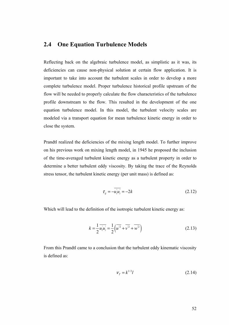
2.4 One Equation Turbulence Models
Reflecting back on the algebraic turbulence model, as simplistic as it was, its
deficiencies can cause non-physical solution at certain flow application. It is
important to take into account the turbulent scales in order to develop a more
complete turbulence model. Proper turbulence historical profile upstream of the
flow will be needed to properly calculate the flow characteristics of the turbulence
profile downstream to the flow. This resulted in the development of the one
equation turbulence model. In this model, the turbulent velocity scales are
modeled via a transport equation for mean turbulence kinetic energy in order to
close the system.
Prandtl realized the deficiencies of the mixing length model. To further improve
on his previous work on mixing length model, in 1945 he proposed the inclusion
of the time-averaged turbulent kinetic energy as a turbulent property in order to
determine a better turbulent eddy viscosity. By taking the trace of the Reynolds
stress tensor, the turbulent kinetic energy (per unit mass) is defined as:
' ' 2ij i iu u kτ = − = − (2.12)
Which will lead to the definition of the isotropic turbulent kinetic energy as:
( )' ' '2 '2 '21 12 2i ik u u u v w= = + + (2.13)
From this Prandtl came to a conclusion that the turbulent eddy kinematic viscosity
is defined as:
1/ 2
T k lν = (2.14)
52

The turbulent kinetic energy in equation 2.14 will be solved through a transport
equation. The transport equation for the turbulent kinetic energy is:
' '
' ' ' ' '1 12
i i ij ij i i j
j j k k j j
U u uk k kU ut x x x x x x
τ ν νρ ju u p u
⎡ ⎤∂ ∂ ∂∂ ∂ ∂ ∂+ = − + − −⎢ ⎥∂ ∂ ∂ ∂ ∂ ∂ ∂⎢ ⎥⎣ ⎦ (2.15)
In order to close for the transport equation for the turbulence kinetic energy, the
Reynolds stress in the production term, the dissipation term and the turbulence
and pressure diffusion term needs to be prescribed. For the Reynolds stress, the
one equation still utilises Boussinesq eddy viscosity approximation.
Since Boussinesq eddy viscosity approximation is still being used to determine
the Reynolds stress, the one model equation still holds the same deficiency of the
algebraic turbulent model in associating mean velocity gradient in shaping the
turbulent property of the flow.
The Prandtl (1945) one-equation model was also attributed to Kolmogorov,
Emmons (1954) and Glushko (1965). Kolmogorov was attributed due to his
involvement in their effort to develop the model. Emmons on the other hand
coincidently proposed the same one equation model in 1954. Apart from the
Prandtl one equation model, a few notably one equation turbulence model was
developed in the 1960s by Bradshaw, Ferriss and Atwell (1967), Nee and
Kovasznay (1968) and Wolfstein (1967 and 1969).
Recent efforts to improve the one equation model have been made by Baldwin et
al. (1990) and Spalart et al. (1992). These one-equation turbulence models are
dubbed complete since the need to prescribed empirical values for the length scale
is no longer needed.
The Spalart-Allmaras turbulence model only showed a slight advantage against
the algebraic turbulence model. Prediction of boundary layer flow near the wall is
within close similarity with the algebraic turbulence model. Separated flow
53

showed a slight better prediction by the Spalart-Allmaras turbulence model over
the algebraic turbulence model. However, the Spalart-Allmaras turbulence model
still suffers from setbacks. It has problems in predicting jet flows, separated and
decaying turbulence flow (Wilcox, 2001).
In summary, it can be said that although it is a good move to include turbulent
kinetic energy as a representation of the turbulent velocity scale, the one equation
model is only slightly better than the algebraic turbulence model and suffer from
the lack of proper modelling of the turbulence length scale. Both zero and one-
equation models are good in modelling isotropic equilibrium flows in region of
low Reynolds number the production of turbulence and dissipation are in balance.
However, in non-equilibrium flows, properly modelling needs to be done to
accommodate the rapid changes in turbulence length scale.
2.5 Two Equation Turbulence Models
In the two-equation turbulence model, in addition to the turbulence velocity scale
(mean turbulence kinetic energy), the turbulence length scale is also modelled via
a transport equation. The modelled turbulence length scale will then be added
together with the mean turbulence kinetic energy in the turbulence eddy viscosity
for a better prediction of the Reynolds stresses using the Boussinesq
approximation. Several version of the modelled turbulence length scale exists and
it will be later explained in this section. Launder et al. (1972a) described the
generalised form of the modelled length scale as:
m nz k l≡ (2.16)
Where m and n are constants.
Kolmogorov proposed the first two-equation model in 1942. Kolmogorov
proposed the z equation to be defined as the specific dissipation rate, ω. Ever
since Kolmogorov postulated his two-equation model, several researchers have
54
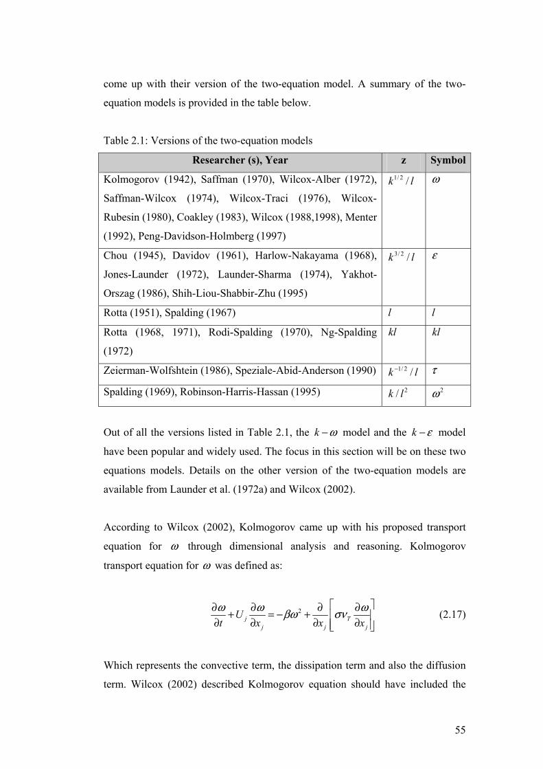
come up with their version of the two-equation model. A summary of the two-
equation models is provided in the table below.
Table 2.1: Versions of the two-equation models
Researcher (s), Year z Symbol
Kolmogorov (1942), Saffman (1970), Wilcox-Alber (1972),
Saffman-Wilcox (1974), Wilcox-Traci (1976), Wilcox-
Rubesin (1980), Coakley (1983), Wilcox (1988,1998), Menter
(1992), Peng-Davidson-Holmberg (1997)
1/ 2 /k l ω
Chou (1945), Davidov (1961), Harlow-Nakayama (1968),
Jones-Launder (1972), Launder-Sharma (1974), Yakhot-
Orszag (1986), Shih-Liou-Shabbir-Zhu (1995)
3/ 2 /k l ε
Rotta (1951), Spalding (1967) l l
Rotta (1968, 1971), Rodi-Spalding (1970), Ng-Spalding
(1972)
kl kl
Zeierman-Wolfshtein (1986), Speziale-Abid-Anderson (1990) 1/ 2 /k l− τ
Spalding (1969), Robinson-Harris-Hassan (1995) 2/k l 2ω
Out of all the versions listed in Table 2.1, the model and the model
have been popular and widely used. The focus in this section will be on these two
equations models. Details on the other version of the two-equation models are
available from Launder et al. (1972a) and Wilcox (2002).
k ω− k ε−
According to Wilcox (2002), Kolmogorov came up with his proposed transport
equation for through dimensional analysis and reasoning. Kolmogorov
transport equation for was defined as:
ω
ω
2j
j j
Ut x x xω ω βω σνT
j
ω⎡ ⎤∂ ∂ ∂ ∂+ = − + ⎢ ⎥∂ ∂ ∂ ∂⎢ ⎥⎣ ⎦ (2.17)
Which represents the convective term, the dissipation term and also the diffusion
term. Wilcox (2002) described Kolmogorov equation should have included the
55

term for production. Although Kolmogorov first postulated that represented
dissipation of the smallest eddies and therefore should not contain a production
term, it was later found out large eddies are actually responsible in determining
the time scale of turbulence, hence the rate of dissipation. Furthermore,
Kolmogorov equation did not include a molecular diffusion term making it only
valid for high Reynolds number flow and cannot be integrated through the viscous
sub-layer region of the flow.
ω
The Kolmogorov equation was then modified and further developed by
researchers (Refer Table 2.1) over the years and the most popular version was the
one by Wilcox (2002), which was defined as:
k ω−
( )
( )
*
* *
2 *
T
ij ij T
j j j j
ij ij T
j j j
k
Uk k kU kt x x x x
UUt x k x x x
ν αω
τ β ω ν σ ν
ω ω ωα τ βω ν σ ν
=
⎡ ⎤∂∂ ∂ ∂ ∂+ = − + +⎢ ⎥∂ ∂ ∂ ∂ ∂⎢ ⎥⎣ ⎦
j
ω⎡ ⎤∂∂ ∂ ∂ ∂+ = − + +⎢ ⎥∂ ∂ ∂ ∂ ∂⎢ ⎥⎣ ⎦
(2.18)
Where the closure coefficients are obtained empirically, Wilcox (2002). Both the
closure coefficients and auxiliary relations are further defined as:
56

( )( )
( )
*
*
* * *
3*
4
*4
2
2
3
* 1/ 2
13 1, , ,25 2
1 709 , ,125 1 80
4 /15 Re /9 , 8100 1 Re /
1, 0, 01 680
1 4001
, /
o o
ij jk kio
o
to
t
k
kk
k
kj j
f f
Sf
RR
R
f
kx x
k l k
β β
ωβ ω
ω
ββ
β
β
α β β β β σ σ
χβ χχ β ω
β
χχχ
χωχ
ω
ε β ω ω
= = = = =
Ω Ω+= = ≡+
⎛ ⎞+⎜ ⎟= =⎜ ⎟+⎝ ⎠≤⎧
⎪= >+⎨⎪ +⎩
∂ ∂≡∂ ∂
= =
(2.19)
*
* *
*
* *
*
Re / R1 Re / R
Re , 6, , 0.0723
1
Re / R1 Re / R
2.95, 0.520.52
o t k
t k
it k o i
o t
t
k R
R
ω
ω
ω
αα α
βρ α βμω
α α
αααα
αα α
∞
∞
∞
∞
∞
⎛ ⎞+= ⎜ ⎟+⎝ ⎠
= = = =
= =
⎛ ⎞+= ⎜ ⎟+⎝ ⎠= == =
(2.20)
The Wilcox turbulence model is an empirical turbulence model and was
first developed as a high Reynolds number turbulence model. It was then later that
a low Reynolds number version of the Wilcox was developed, Wilcox
(2002), Fluent (2003).
k ω−
k ω−
As with the k turbulence model, the turbulence model exists in many
versions. Jones et al. developed the current standard version of the
turbulence model in 1972, Launder et al. (1972a). The model of Jones and
Launder was developed for high Reynolds number application but accounted for
low Reynolds number effects as well. Launder et al. (1974) later improved the
ω− k ε−
k ε−
57

k ε− turbulence model of Jones et al. (1972) by modifying its closure coefficients
and damping functions for low Reynolds number application, Wilcox (2002).
However, despite being very popular and widely used, the standard
turbulence model has its deficiencies, which will be discussed later in this section.
This led to the development of several improved version of the turbulence
models designed to overcome the deficiencies of the standard turbulence
model. Such models that will be discussed in this section are the RNG
turbulence model by Yakhot et al. (1986) and the Realizable turbulence
model by Shih et al. (1995).
k ε−
k ε−
k ε−
k ε−
k ε−
The standard turbulence model is defined as: k ε−
( )
( )
( )
2
2
1 2
1 2
3/ 2
/
/
/
1.44, 1.92, 0.09, 1.0, 1.3
/ , /
T
ij ij T k
j j j j
ij ij T
j j j j
k
C k
Uk k kUt x x x x
UU C Ct x k x k x
C C C
C k l C k
μ
ε ε
ε ε μ ε
μ μ
ν ε
τ ε ν ν σ
ε ε ε ετ ν σ
σ σ
ω ε ε
=
⎡ ⎤∂∂ ∂ ∂ ∂+ = − + +⎢ ⎥∂ ∂ ∂ ∂ ∂⎢ ⎥⎣ ⎦
xεεν
⎡ ⎤∂∂∂ ∂ ∂+ = − + +⎢ ⎥∂ (2.21)
∂ ∂ ∂ ∂ ⎢ ⎥⎣ ⎦= = = =
= =
The turbulence model predicts the kinematic eddy viscosity value through
the modelling of the turbulence velocity and length scale. This is achieved by
solving additional transport equation of mean turbulent kinetic energy (velocity
scale) and dissipation rate (length scale).
k ε−
Over the years the standard turbulence model have proved to be both
economical and robust. However, it has its deficiencies, such as the inability to
predict highly strained flow, swirling flow, rotating and separating flow, Naser
(2003). However, due to the deficiencies of the standard turbulence model,
improvements have been made to overcome such setbacks, which lead to the
development of the RNG model and the Realizable k model.
k ε−
ε
k ε−
ε−k −
58
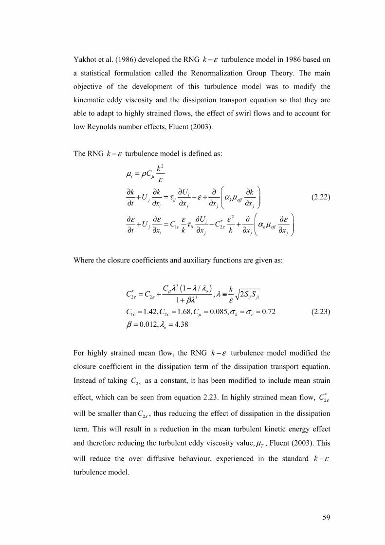
Yakhot et al. (1986) developed the RNG turbulence model in 1986 based on
a statistical formulation called the Renormalization Group Theory. The main
objective of the development of this turbulence model was to modify the
kinematic eddy viscosity and the dissipation transport equation so that they are
able to adapt to highly strained flows, the effect of swirl flows and to account for
low Reynolds number effects, Fluent (2003).
k ε−
The RNG turbulence model is defined as: k ε−2
2*
1 2
t
ij ij k eff
i j j j
ij ij k eff
i j j
kC
Uk k kUt x x x x
UU C Ct x k x k x x
μ
ε ε
μ ρε
τ ε α μ
ε ε ε ετ α
=
⎛ ⎞∂∂ ∂ ∂ ∂+ = − + ⎜ ⎟⎜ ⎟∂ ∂ ∂ ∂ ∂⎝ ⎠⎛ ⎞∂∂ ∂ ∂ ∂+ = − + ⎜ ⎟⎜ ⎟∂ ∂ ∂ ∂ ∂⎝ ⎠j
εμ
(2.22)
Where the closure coefficients and auxiliary functions are given as:
( )3*2 2 3
1 2
1 /, 2
11.42, 1.68, 0.085, 0.72
0.012, 4.38
oij ji
k
o
C kC C S S
C C C
με ε
ε ε μ ε
λ λ λλ
βλ εσ σ
β λ
−= + ≡
+= = = = =
= =
(2.23)
For highly strained mean flow, the RNG turbulence model modified the
closure coefficient in the dissipation term of the dissipation transport equation.
Instead of taking as a constant, it has been modified to include mean strain
effect, which can be seen from equation 2.23. In highly strained mean flow,
will be smaller than , thus reducing the effect of dissipation in the dissipation
term. This will result in a reduction in the mean turbulent kinetic energy effect
and therefore reducing the turbulent eddy viscosity value,
k ε−
2C ε
2C
*2C ε
ε
Tμ , Fluent (2003). This
will reduce the over diffusive behaviour, experienced in the standard
turbulence model.
k ε−
59

As with the standard k turbulence model, the RNG turbulence model
take into account for low Reynolds number effects. The diffusion term on both
transport equation was modified for this matter. For low Reynolds number flow,
the integration of equation 2.24 and the inverse effective Prandtl numbers, and
is used to account for the varying Reynolds number. The calculation from
equation 2.24 will then be incorporated into the diffusion term for both transport
equation, and will also be used to determine the value for the turbulence eddy
viscosity,
ε− k ε−
kα
εα
Tμ . For high Reynolds number flow, the default Tμ from equation 2.22
will be used.
2
3
0.6321 0.3679
ˆ ˆ ˆ1.72 , , 100ˆ 1
1.3929 2.39291.3929 2.3929
1.0
1, 1.393
eff
o o eff
o
keff
kd dC
νν
ε
μρ ν ν νμεμ ν
α α μα α μαμ α αμ
⎛ ⎞= =⎜ ⎟⎜ ⎟ − +⎝ ⎠
− + =− +
=
= ≈=
C ≈
(2.24)
For swirling effects, the RNG turbulence model incorporates the function
from equation 2.25 into the turbulence eddy viscosity,
k ε−
Tμ .
⎟⎠⎞
⎜⎝⎛ Ω=
εαμμ kf sot ,, (2.25)
Where oμ can be taken from either high or low Reynolds number flow
formulation for turbulence eddy viscosity, Tμ .
However, although the RNG turbulence model is an improvement from the
standard turbulence model, it still has its limitations. This is due to the
transport equation for the dissipation term, . Because of the fact that the
k ε−
k ε−
ε
60

transport equation for the dissipation term is derived based on physical reasoning
and dimensional analysis alone, certain mathematical limitation will exist and
needs to be satisfied in order to be consistent with the prediction of Reynolds
stresses, hence the turbulence flow, Fluent (2003). The RNG and standard
turbulence model does not satisfy these mathematical limitations, making them
not ‘Realizable’. Due to this fact, Shih et al. developed the Realizable
turbulence model in 1995 to address these mathematical limitations and improve
on it. From their research, they have developed a new transport equation for the
dissipation term from the exact equation based on the mean-square vorticity
fluctuation transport equation, Shih et al. (1995). In addition, they also modified
the formulation for the turbulence eddy viscosity term,
k ε−
k ε−
Tμ , by improvising on the
closure constant Cμ , varying it in order to adjust to different flow applications.
The Realizable turbulence model is defined as: k ε−
( )
( )
2
2
1 2
/
/
/
T
ij ij T k
j j j j
j Tj j
C k
Uk k kUt x x x x
U C S Ct x x xk
μ
ε
ν ε
τ ε ν ν σ
ε ε ε εε ν ν σνε
=
⎡ ⎤∂∂ ∂ ∂ ∂+ = − + +⎢ ⎥∂ ∂ ∂ ∂ ∂⎢ ⎥⎣ ⎦ (2.26)
⎡ ⎤∂ ∂ ∂ ∂+ = − + +⎢j⎥∂ ∂ ∂ ∂+ ⎢ ⎥⎣ ⎦
Where the closure coefficients and the formulation for Cμ are defined as:
( )
1 2
*
~1
~
*
max 0.43, , , 1.9, 1.0, 1.25
1 , 4.04, 6 cos ,
1 1cos 6 , , ,3 2
k
o s
o s
ij jk ki jiij ij ij
j i
ij ij ij ij
ij ij ijk k
kC S C
C A AkUA A
S S S UUW W S S S Sx xS
U S S
ε
μ
η η σ ση ε
φ
ε
φ
ε ω
−
⎡ ⎤= = = = =⎢ ⎥+⎣ ⎦
= = =+
⎛ ⎞∂∂= = = = +⎜ ⎟⎜ ⎟∂ ∂⎝ ⎠
≡ +Ω Ω
Ω = Ω −
(2.27)
61
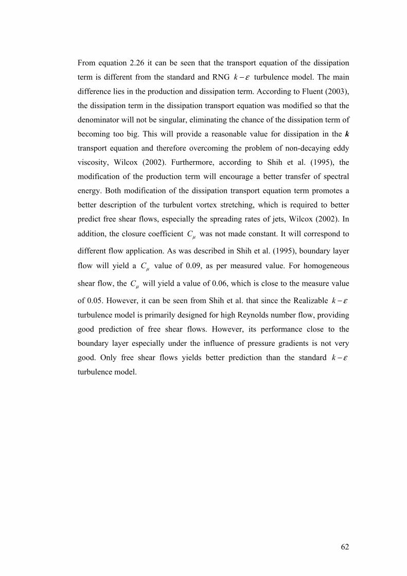
From equation 2.26 it can be seen that the transport equation of the dissipation
term is different from the standard and RNG turbulence model. The main
difference lies in the production and dissipation term. According to Fluent (2003),
the dissipation term in the dissipation transport equation was modified so that the
denominator will not be singular, eliminating the chance of the dissipation term of
becoming too big. This will provide a reasonable value for dissipation in the k
transport equation and therefore overcoming the problem of non-decaying eddy
viscosity, Wilcox (2002). Furthermore, according to Shih et al. (1995), the
modification of the production term will encourage a better transfer of spectral
energy. Both modification of the dissipation transport equation term promotes a
better description of the turbulent vortex stretching, which is required to better
predict free shear flows, especially the spreading rates of jets, Wilcox (2002). In
addition, the closure coefficient
k ε−
Cμ was not made constant. It will correspond to
different flow application. As was described in Shih et al. (1995), boundary layer
flow will yield a Cμ value of 0.09, as per measured value. For homogeneous
shear flow, the Cμ will yield a value of 0.06, which is close to the measure value
of 0.05. However, it can be seen from Shih et al. that since the Realizable
turbulence model is primarily designed for high Reynolds number flow, providing
good prediction of free shear flows. However, its performance close to the
boundary layer especially under the influence of pressure gradients is not very
good. Only free shear flows yields better prediction than the standard
turbulence model.
k ε−
k ε−
62

2.6 Deficiencies of the Two Equation Turbulence Model
Deficiency of the two-equation model can be traced to three main reasons, which
is the inability to predict flow in the presence of pressure gradient close to the
wall and due to the inability to take into account the effect of rapid change in
mean strain rate due to the sharp streamline curvature of the geometry.
2.6.1 Pressure Gradient Effects
The two-equation model, especially the k-ε still fail to accurately predict flow in
the boundary layer region, close to the wall even after treating it. Perturbation of
the defect layer then showed that the reason for this was due to large turbulence
scale developed close to the boundary layer especially in the presence of adverse
pressure gradient effect. Analysis by Wilcox (2002) showed that by adding a cross
diffusion term to the k-ε turbulence model, the increase of the turbulence scale
close to the wall could be suppressed. Furthermore, analysis of wake Coles et al.
(1969) wake strength parameter in the defect layer against a function of pressure
gradient showed that as adverse pressure gradient effect increases close to the
wall, the wake strength parameter was being under predicted as a result of an
increase in skin friction coefficient close the wall.
According to Rodi et al. (1986), two-equation turbulence model perform badly in
region close to the wall due to the fact that the dissipation length scale rises
sharply near the wall. However, Bradshaw (1969) have shown through
experimental data that the dissipation length scale is independent in the region
close to the wall. Coles et al. (1969) also supported this and described that the
turbulent boundary layer close to the wall exists in different scales and physical
processes. Rodi et al. (1986) also suggest that under adverse pressure gradient, the
rate of kinetic energy production is more than the rate of dissipation itself,
resulting in an increase in turbulence dissipation length scale. This will lead to an
increase and over prediction of turbulent eddy viscosity and wall shear stress.
63

However, although the k-ε versions of the two-equation model have proved
inaccurate in predicted a wide range of flow due to its deficiencies, the k-ω
turbulence model developed by Wilcox (2002) have proved to be rather
successful. Part of the reason is the presence of the cross diffusion term in the k-ω
as a way to suppress the increase of the turbulence dissipation length scale close
to the wall. However, the addition of cross diffusion term can cause instability to
the calculation of the flow, since it augments the influence of convection in the
flow. Therefore, treatment is needed to curb this instability, Wilcox (2002). The k-
ω turbulence model prediction of boundary layer flow only differ by 3.5% from
measurement and have shown to predict separation rather successfully as well.
However, a minor setback of the k-ω turbulence model is that the sub-layer region
has to be integrated which means grid generation near the wall must be
sufficiently fine.
2.6.2 Effect of Rapid change of Mean Strain Rate and
Streamline Curvature
According to Wilcox (2002), the main flaw of the eddy viscosity model, which
assumes Boussinesq approximation is the fact that it assumes the Reynolds stress
are proportional to the mean strain rate at all part of the flow, a postulation from
Stokes based on laminar flows. The constant of proportionality was defined as the
eddy turbulent viscosity. However, turbulent flow is affected by the change of
geometry, anisotropy and flow history. With the presence of curvature in the flow,
the individual Reynolds stress values will be different and hence, again the
Boussinesq assumptions will become flawed, Wilcox (2002).
Bradshaw (1973) described that eddy-viscosity models offers inaccurate
prediction of flows that undergo rapid changes in rates of strain. The main reason
for this is because the adjustment of Reynolds stresses to such changes is
unrelated to turbulence mean flow and time scale effect.
64

Therefore, the effect of curvature can be treated either by making correction to the
two-equation models. Alternatively, the Reynolds Stress Transport model can be
used. Naser (1990) described from Bradshaw (1973) that since the effect of
curvature causes large changes in the Reynolds stresses and triple velocity
correlations, the Boussinesq assumptions must be corrected. Bradshaw (1973)
proposed that the extra effect of strain rate would modify the Boussinesq
assumption to include a factor of an order of magnitude higher. Therefore, the
Reynolds stresses from the Boussinesq assumption will be modeled as:
' ' Tu vu vy x
ν α⎛ ⎞∂ ∂= +⎜ ∂ ∂⎝ ⎠⎟ (2.28)
Where is of the order of 10. α
Modifying certain aspect in the two-equation turbulence model can also treat the
effect of flow curvature. Leschnizer et al. (1981) made modifications in the Cμ to
take into account the effect of curvature and obtained good prediction in parallel
jet flow. Furthermore, Bradshaw (1969) proposed a dimensionless number that
takes into account the curvature effect. Sharma (1975) and Launder et al. (1977)
modified the dissipation equation in the k-ε to take into account the curvature
effect. With that respect, they modified the . Rodi (1979) made corrections in
the constant. Finally, Wilcox et al. (1977) proposed a correction to the k-ω
turbulence model within the k equation term and the logarithmic law equation.
2Cε
1Cε
2.7 Reynolds Stress Turbulence Models
Deficiencies of the eddy viscosity turbulence model inspired early turbulence
models developer such as Chou (1945) and Rotta (1951) to propose a turbulence
model where the Reynolds stresses, i ju u− are not modeled through the
Boussinesq assumption and the Reynolds stresses, are solved directly through a
set of transport equations. This turbulence model is known as the Reynolds Stress
65

Turbulence Model (RSM) or second order/moment closure. According to Wilcox
(2001), such early contributors to the development of the RSM include Donaldson
et al. (1968), Daly et al. (1970), Launder et al. (1975), Gibson et al. (1978),
Lumley (1978), Speziale (1985, 1987a, 1991) and Reynolds (1987). Throughout
the years, Launder et al. (1975) RSM have became the one of the most popular
and have been set as a baseline for RSM.
The direct use of Reynolds stresses to for turbulence modeling, especially in a
three-dimensional flow, generates six extra transport equations, which represents
the individual components of the Reynolds stresses. In addition, a transport
equation is also used to solve for the turbulence length scale and this is normally
employed through the use of the dissipation transport equation, . ε
The transport equation for Reynolds stress from Wilcox (2002), is given as:
' '' ' ' '
' ' '2ij ij j j j iji i ik ik jk i j k
k k k k k j i k k
U u uU u u p pU ut x x x x x x x x xτ τ τ
τ τ ν νρ ρ
∂ ∂ ∂ ∂ ∂u u
⎡ ⎤∂ ∂ ∂ ∂ ∂+ = − − + + + + +⎢ ⎥∂ ∂ ∂ ∂ ∂ ∂ ∂ ∂ ∂ ∂⎣ ⎦ (2.29)
Equation 2.29 consists of convective term on the left hand side of the equation.
The first two terms on the right hand side of the equation is the production term,
followed by the dissipation term, two pressure strain redistribution term and the
diffusion term. For a three-dimensional flow, the six extra Reynolds stress
transport equations generate extra 22 unknowns. Ten unknowns generated are in
the form of triple velocity correlation that forms the turbulent diffusion term. A
further six unknowns are generated from the dissipation term and six more
unknowns from the pressure strain distribution term, Wilcox (2002).
According to AVL (2003), the extra unknowns generated are of higher order
correlations and the main challenge in Reynolds stress modelling is to model these
unknowns. The terms that need to be modelled consists of the dissipation term,
the turbulent diffusion term and the pressure strain redistribution term. According
to Wilcox (2002), the resulting Reynolds stress equation will be:
66

ij ij ijk ij ij ij ijk
k k
U P Ct x x xτ τ τ
ε ν∂ ∂ ∂
k
⎡ ⎤∂+ = + −Π + +⎢ ⎥∂ ∂ ∂ ∂⎣ ⎦ (2.30)
here the production and are given as: W , ,ij ij ijP ε Π ijkC
''
'''
' ' ' ' ' ' '
2
j iij ik jk
k k
jiij
k k
jiij
j i
ijk i j k i jk j ik
U UPx x
uux x
uupx x
C u u u p u p u
τ τ
ε ν
ρ
ρ ρ δ δ
∂ ∂= − −∂ ∂
∂∂=∂ ∂
⎛ ⎞∂∂Π = +⎜ ⎟⎜ ⎟∂ ∂⎝ ⎠
= + +
(2.31)
hich consists of the production term, the dissipation term, the pressure strain
ccording to Wilcox (2002), the Reynolds stress component in the production
he dissipation term, is modelled based on high Reynolds number flow
W
redistribution term and the turbulent diffusion (triple velocity correlation) term.
A
term, ijP , is solved through the Reynolds stress transport equation.
T ijε ,
conditions where the effect of ijε can be assumed to be isotropic (Hanjalic et al.,
1976) and is defined as:
23ij ijε ε= δ (2.32)
Where, ijδ , is the boundary layer thickness, which accounts for the effects of near
wall anisotropy. The transport equation used to solve for ε is similar to the
dissipation transport equation from the standard ε−k turbulence model. Hanjalic
et al. (1972) and Launder et al. (1975) defined the nsport equation for ir tra ε as:
67

2
1 2ik i
kmk m k
UD kC CDt x x k x kε ε
ετε ετε⎡ ⎤ ∂∂ ∂= −⎢ ⎥∂ ∂ ∂⎣ ⎦
Cεε− (2.33)
he turbulent diffusion term, ijkCρ ,T which consists of higher order velocity
fluctuation correlation components was firstly modelled by Daly et al. (1970)
using a simple gradient-diffusion hypothesis, which defines ijkC to be:
' ijijk s km
m
kC Cxτ
τε
∂=
∂ (2.34)
Hanjalic et al. (1972) and Launder et al. (1975) proposed another version of the
modelled ijkC term, which was defined as:
jk ijkiijk s im jm km
m m
kC Cmx x x
τ τττ τ τε
∂ ∂⎛ ⎞∂= + +⎜ ⎟∂ ∂ ∂⎝ ⎠ (2.35)
The constants and 'sC sC are given approximately as 0.25 and 0.11 respectively.
However, according to Lien et al. (1994), the equation derived in 2.34 and 2.35
might have destabilising effect especially in three-dimensional flows. Therefore,
an isotropic version of ijkC is provided and defined as:
'2
ijk skvC Cε
≡ (2.36)
Where was defined as 0.22 and '2sC 0.361v k≅ .
hir (1973) have also come up with a simple gradient diffusion concept, in which
S
ijkC is defined as:
68

2ij
ijk sk
kC Cxτ
ε∂⎛ ⎞
= ⎜ ∂⎝ ⎠⎟ (2.37)
The last term that requires modelling for the Reynolds stress turbulence model is
the pressure strain term. According to Wilcox (2002), the pressure strain term is
the term that received the most attention. The reason for this is because since the
pressure strain term has the same order as the production term, it plays an
important role in the majority of engineering flows of interest. In addition, the
pressure strain term requires some degree of creativity to model in order to
achieve approximate closure.
For homogeneous turbulence, the pressure strain term is divided into two parts, a
slow fluctuating pressure and a rapid fluctuating pressure.
,1 ,2ij ij ijφ φΠ = + (2.38)
Where the first term on the right hand side of equation 2.38 represents the slow
pressure strain rate term and the second term represents the rapid pressure strain
term.
Rotta (1951) postulated that the slow pressure term could be modelled linearly as:
,1 123ij ij ijC
kε kφ τ δ⎛= − +⎜⎝ ⎠
⎞⎟ (2.39)
Where C1 is a closure coefficient obtained from the empirical measurement of
Uberoi (1956) to lie between 1.4 < C1 < 1.8.
Launder et al. (1975) proposed a model to solve for the rapid pressure strain
redistribution term based on the analysis of Rota (1951), which is strictly valid
only for homogeneous turbulence. Gibson et al. (1978) then proposed a simplified
69

version of the Launder et al. (1975) model, which defines the rapid pressure strain
redistribution term as:
,2 223ij ij ij
j iij ik jk
k k
iik
k
C P P
U UPx x
UPx
φ δ
τ τ
τ
⎛ ⎞= − −⎜ ⎟⎝ ⎠∂ ∂≡ − −∂ ∂∂≡ −∂
(2.40)
Speziale et al. (1991) have developed a simple, non-linear pressure strain
redistribution model for incompressible flow, which is often called as the SSG
quadratic pressure strain model. The SSG model has become a popular choice
among pressure strain redistribution model since it does not require a correction
for the near wall reflection effect (will be explained in the following section). The
SSG model is defined as:
( )( )
*1 1 2
*3 3 4
5
13
23
mij mn ij ik kj mn nm ij
n
ij ij ij ik jk jk ik mn mn ij
ik jk jk ik
UC C b C b b b bx
C C b b kS C k b S b S b S
C k b b
ε τ ε δ
δ
⎛ ⎞∂ ⎛ ⎞Π = − + + −⎜ ⎟ ⎜ ⎟∂ ⎝ ⎠⎝ ⎠⎛ ⎞+ − + + −⎜ ⎟⎝ ⎠
+ Ω + Ω
(2.41)
Where, , is defined as: ijb
13ij kk ij
ijmm
bτ τ δ
τ
−≡ (2.42)
And the constants are given as:
* *
1 1 2 3 3 4 53.4, 1.8, 4.2, 0.8, 1.3, 1.25, 0.4C C C C C C C= = = = = = =
70

The main advantage of the RSM is that it takes into account the anisotropic nature
of turbulence in predicting flows by incorporating non-local and history effect of
turbulence, Ahmed (1998), Wilcox (2002). Due to this, RSM provide better
prediction of flow over streamline curvature, swirling flows, rotation, and flow
with rapid changes in the mean strain rate, FLUENT (2003). According to Wilcox
(2002), unlike eddy viscosity turbulence models, which uses treatment and
compensation through the manipulation of mathematical formulation to predict
complex flows, the RSM provides better prediction of complex flow in a more
natural way by direct modeling of the Reynolds stresses.
Furthermore, according to AVL (2003), RSM modeling of each individual stress
component enables accurate prediction of anisotropic turbulence, which often
plays a crucial role as a major source of energy in complex flows, such as in
stagnation regions, secondary motion and in vortex flows. RSM also provide
accurate prediction of the unequal wall-normal stress component, which is
important in reproducing wall shear stress and mass transfer close to the wall.
However, despite the advantages that have been showed by the RSM in predicting
complex flows, it does not offer any superiority over eddy viscosity models in
predicting free stream flows and boundary layer flow and it also share the
shortcomings experienced by the eddy viscosity model especially in poor
prediction of three dimensional and separated flow. This deficiency can be traced
back on the modelling of higher correlation terms such the pressure strain
redistribution term and also on the modelling turbulence length scale through the
dissipation ( ) term, Wilcox (2002), FLUENT (2003). According to Wilcox
(2002) the usage of the dissipation term in predicting the turbulence length scale
will inadvertently transfer the deficiency of the two equation eddy viscosity
models to the Reynolds stress turbulence model. Wilcox (2002) has also shown
from the DNS simulation of Parneix et al. (1998) that deficiency of the RSM can
also be traced back through the modelling of the pressure strain rate correlation.
The DNS simulation showed inaccurate results was obtained despite accurate
modelling of dissipation, . The inability for Reynolds stress turbulence model to
provide better prediction for three-dimensional flows can be traced back on the
ε
ε
71

application of two-dimensionality in boundary layer flows. According to AVL
(2003), current turbulence models have been developed based on the knowledge
of two-dimensional flows. In three-dimensional boundary layer, the eddy
viscosity is not isotropic. Latest work of Schwarz et al. (1994) has studied the
performance of some Reynolds stress turbulence model in three-dimensional
boundary layer flow. Based on their findings, they have concluded that the main
cause of error in the performance of RSM models in a three dimensional boundary
layer is due to the inadequacy of the modelling of dissipation.
A new and attractive alternative to the RSM is the use of hybrid turbulence model
that incorporates attributes from the eddy viscosity two-equation models and the
RSM. The hybrid turbulence model offer the advantages of the RSM turbulence
model in terms of its accuracy and its applicability over curved flows and at the
same time offer the robustness and convergence speed of the eddy viscosity two
equation model. For this instance, Basara et al. (2003) proposed a hybrid
turbulence model (HTM) that combines both the advantages and applicability of
the RSM and turbulence models. In the HTM model proposed by Basara et
al. (2003), the solution for the Reynolds stress is obtained form the Boussinesq
assumption of equating stress to the mean strain of the flow (equation 2.10). The
solution for the turbulence eddy viscosity is obtained similarly from the k-epsilon
model (equation 2.73). The calculation of k and to solve for the turbulent eddy
viscosity is obtained similarly from the RSM turbulence model (Refer the AVL
use of RSM turbulence model). The k equation obtained from the summation of
normal Reynolds stresses. The dissipation term is solved from the transport
equation for dissipation. The main difference in the HTM turbulence model is the
k ε−
ε
Cμ constant used in defining the turbulent eddy viscosity. Cμ is defined by:
2
2/ , 2ii j ij ij
j
U kC u u S S Sxμ ε
⎛ ⎞ ⎛ ⎞∂= − =⎜ ⎟ ⎜ ⎟⎜ ⎟∂ ⎝ ⎠⎝ ⎠S (2.43)
Which is the ratio between the RSM production term and the k production
term. The rationale from the variable value of C
ε−
μ is due to the fact that according
72
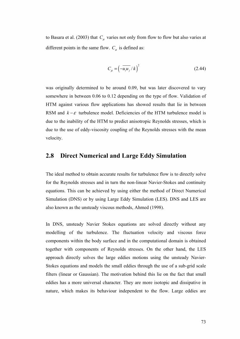
to Basara et al. (2003) that Cμ varies not only from flow to flow but also varies at
different points in the same flow. Cμ is defined as:
( 2/i jC u u k )= − (2.44) μ
was originally determined to be around 0.09, but was later discovered to vary
somewhere in between 0.06 to 0.12 depending on the type of flow. Validation of
HTM against various flow applications has showed results that lie in between
RSM and turbulence model. Deficiencies of the HTM turbulence model is
due to the inability of the HTM to predict anisotropic Reynolds stresses, which is
due to the use of eddy-viscosity coupling of the Reynolds stresses with the mean
velocity.
k ε−
2.8 Direct Numerical and Large Eddy Simulation
The ideal method to obtain accurate results for turbulence flow is to directly solve
for the Reynolds stresses and in turn the non-linear Navier-Stokes and continuity
equations. This can be achieved by using either the method of Direct Numerical
Simulation (DNS) or by using Large Eddy Simulation (LES). DNS and LES are
also known as the unsteady viscous methods, Ahmed (1998).
In DNS, unsteady Navier Stokes equations are solved directly without any
modelling of the turbulence. The fluctuation velocity and viscous force
components within the body surface and in the computational domain is obtained
together with components of Reynolds stresses. On the other hand, the LES
approach directly solves the large eddies motions using the unsteady Navier-
Stokes equations and models the small eddies through the use of a sub-grid scale
filters (linear or Gaussian). The motivation behind this lie on the fact that small
eddies has a more universal character. They are more isotopic and dissipative in
nature, which makes its behaviour independent to the flow. Large eddies are
73

highly anisotropic and unsteady in nature, which makes it dependent to the flow,
Ahmed (1998).
However, according to Ahmed (1998), the LES approach is a more preferred
option for technical flows because it requires significantly less computer capacity
than DNS, and yet at the same time promises to be more accurate and robust than
the conventional RANS approach.
At the moment, DNS is used purely for research purposes. According to Wilcox
(2002), current DNS application is mostly limited to Low Reynolds number in
two dimensional and simple three-dimensional flows (incompressible and
compressible) with homogeneous turbulence. The extremely high demand that
DNS put on computational capacity leads back to the extremely high grid
generation needed to resolve all turbulent scale (even the smallest Kolmogorov
turbulence scale) in both spatial and temporal dimension.
According to Ahmed (1998), DNS requires grid points that increase with 94
power of Reynolds number. It has been estimated that to capture the effect of the
smallest turbulence motion and solves the flow around a structure the size of a
vehicle, grid points around 1018 would be needed. By the mid 1990s, the largest
number of grid points that could be handled computationally was only around 106,
which makes it so impractical in using DNS vehicle aerodynamics in the
immediate future, Barnard (1996).
Due to this, the approach of using LES is better suited than using DNS. According
to Wilcox (2002) and FLUENT (2003), LES grid size can be at least one order of
magnitude smaller than DNS. Furthermore, a large time step can be used with
flow achievable at a higher Reynolds number. Available LES models are from the
Smagorinsky (1963) simple gradient-diffusion model, the Lilly (1966) one
equation model and the second order closure of Deardorff (1973).
74

2.9 CFD Near Wall Treatment and Boundary
Conditions
Turbulence models discussed in the preceding section was mainly developed for
flows of high Reynolds number values. For laminar boundary layer flow near to
the wall, molecular viscous effects that dominate the turbulent eddy viscosity
must be accounted for, Ahmed (1998). According to Wilcox (2002), one of the
main reason for high Reynolds number turbulence model (most two-equation,
HTM and RSM models) inability to predict accurate values for flow near the wall
especially in the presence of adverse pressure gradients was traced down to the
inaccurate reproduction of the law of the wall constant, C. Analysis showed that
in the example of a standard turbulence model, predicted C value of –2.2 as
oppose to the measured value of 5.0. In another analysis conducted by Rodi et al.
(1986), the deficiency of high Reynolds number turbulence model can be traced
back to the deficiency in the model of the dissipation rate, to predict an accurate
length scale value near to the wall. According to Rodi et al. (1986), for most high
Reynolds number turbulence model, the production of turbulence kinetic energy,
and length scale near to the wall is too steep, resulting from a lower production
in the rate of dissipation. This will result in a high value of Reynolds stresses near
the wall region. In order to overcome this problem, proper treatment is needed to
compensate for this deficiency, for a more reliable near wall prediction.
k ε−
ε
k
Two different approaches are often used for near wall treatment. They are:
• Wall Function approach
• Low Reynolds Number Model approach
75
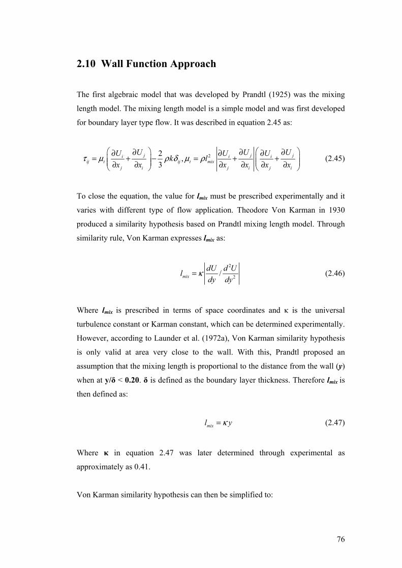
2.10 Wall Function Approach
The first algebraic model that was developed by Prandtl (1925) was the mixing
length model. The mixing length model is a simple model and was first developed
for boundary layer type flow. It was described in equation 2.45 as:
22 ,3
j ji iij t ij t mix
j i j i j i
U UU Uk l ji UUx x x x
τ μ ρ δ μ ρ⎛ ⎞ ⎛ ⎞∂ ∂∂ ∂= + − = + +⎜ ⎟ ⎜⎜ ⎟ ⎜∂ ∂ ∂ ∂ ∂ ∂⎝ ⎠ ⎝ ⎠x x
∂∂⎟⎟ (2.45)
To close the equation, the value for lmix must be prescribed experimentally and it
varies with different type of flow application. Theodore Von Karman in 1930
produced a similarity hypothesis based on Prandtl mixing length model. Through
similarity rule, Von Karman expresses lmix as:
2
2/mixdU d Uldy dy
κ= (2.46)
Where lmix is prescribed in terms of space coordinates and κ is the universal
turbulence constant or Karman constant, which can be determined experimentally.
However, according to Launder et al. (1972a), Von Karman similarity hypothesis
is only valid at area very close to the wall. With this, Prandtl proposed an
assumption that the mixing length is proportional to the distance from the wall (y)
when at y/δ < 0.20. δ is defined as the boundary layer thickness. Therefore lmix is
then defined as:
mixl κ= y (2.47)
Where κ in equation 2.47 was later determined through experimental as
approximately as 0.41.
Von Karman similarity hypothesis can then be simplified to:
76

* lnuU yκ
= +C (2.48)
The constant C can be further evaluated to be:
*
*
1 1ln lnu yUu
βκ ν κ
= − (2.49)
Where, *
Uu
, is the ratio of the mean flow to the friction velocity and is defined as
u+. *u yν
, is the dimensionless distance from the wall and is defined as y+.
Equation 2.49 is famously known as the law of the wall or the universal velocity-
distribution law. Therefore, equation 2.49 can be simplified further to be:
1 ln 5.0u yκ
+ += + (2.50)
The first and the most common approach in treating near wall effect are by using
the wall function approach of Launder et al. (1974). The wall function approach
uses a semi-empirical model, which assumes the behaviour of fluid flow near the
wall to follow the law of the wall profile, which will enforce the proper value for
C in the wall region. Another advantage for using the wall function approach is a
shortened computational time since the steep flow gradients occurring in the sub-
layer region does not need to be resolved. This allow for coarse grid to be
generated close to the wall. For the first cell next to the wall, the wall function
approach automatically assumes a law of the wall profile, which is valid in the
region of y+ < 30 to 500, Roberson et al. (1997). The wall function approach of
Launder et al. (1974) is defined as:
1/ 4 1/ 2
1/ 4 1/ 2 1 ln/
PPP P
w
C kU C k Ey μμτ ρ κ ν
⎛ ⎞= ⎜ ⎟⎜ ⎟
⎝ ⎠ (2.51)
77

Where, E is given as the wall roughness, which is equal to 9.0 for a smooth wall,
Launder et al. (1974). In order to evaluate for the kinetic turbulence energy near
the wall, , the average energy dissipation rate is deduced from the following
equation:
pk
( )1/ 21/ 2
3/ 2
0
lnPY
P PP
Ey C kkdy Cμ
μεκ ν
⎡ ⎤⎢ ⎥= ⎢ ⎥⎢ ⎥⎣ ⎦
∫ (2.52)
In addition, for y+ < 11.225, a laminar stress-strain relationship is used and is
defined as:
1/ 4 1/ 2
1/ 4 1/ 2
/PP
P Pw
C kU C k y μμτ ρ ν
= (2.53)
However, the standard wall function has its disadvantages. According to FLUENT
(2003), due to the fact that the standard wall function was developed from two-
dimensional flow (Ahmed, 1998) and rely on ideal conditions (constant shear and
local turbulent equilibrium), its will yield inaccurate results when conditions
deviate too much from ideal. The wall function approach does not perform very
well in conditions of severe pressure gradients close to the wall, highly three-
dimensional flow close to the wall and where turbulent effect is strongly non-
equilibrium. Throughout the years, improved versions of the standard wall
function have been developed to include non-equilibrium and pressure gradient
effects, which offer better prediction for complex flows that includes separation
and reattachment, FLUENT (2003).
Kim et al. (1995) developed such wall function approach, often known as the non-
equilibrium wall function. The wall function model can withstand non-
equilibrium flow and pressure gradient effects and was developed based on a two-
layer model concept proposed by Chieng et al. (1980) and Launder (1988). Cells
78

adjacent to the wall are assumed and divided into a viscous sub layer and a fully
turbulent layer. The non-equilibrium wall function is defined as:
~ 1/ 4 1/ 2
1/ 4 1/ 2 1 ln/w
C kU C k Ey μμτ ρ κ ν
⎛ ⎞= ⎜ ⎟⎜ ⎟
⎝ ⎠ (2.54)
Where, , takes into account the pressure gradient effect and is defined as: ~
U
2~
1/ 4 1/ 4
1 ln2
v
v
y y ydp y yU Udx yC k C kμ μ
v
μρκ ρκ
⎡ ⎤⎛ ⎞ −= − + +⎢ ⎥⎜ ⎟⎢ ⎥⎝ ⎠⎣ ⎦
(2.55)
And the sub-layer thickness, vy is defined as:
*
*1/ 4 1/ 2
*v
v vP
y
v
y yC k
eyE
μ
κ
ν≡
=
(2.56)
Furthermore, the turbulent kinetic energy, k, is defined as:
2
,
,
P vv
P v
y k y yk y
k y y
⎧ ⎫⎛ ⎞⎪ ⎪<⎜ ⎟= ⎨ ⎬⎝ ⎠⎪ ⎪>⎩ ⎭
(2.57)
According to Makowski et al. (2000), the non-equilibrium wall function is
recommended for vehicle aerodynamic computations because it compensate for
higher than ideal values of y+ near to the wall and also account for the effects of
the variation in wall adjacent grid when computing for the turbulence kinetic
energy, near to the wall. Furthermore, the non-equilibrium wall function provides
a more realistic prediction of the behaviour of turbulent boundary layers
(including separated flow) without increasing significant computational resources.
79
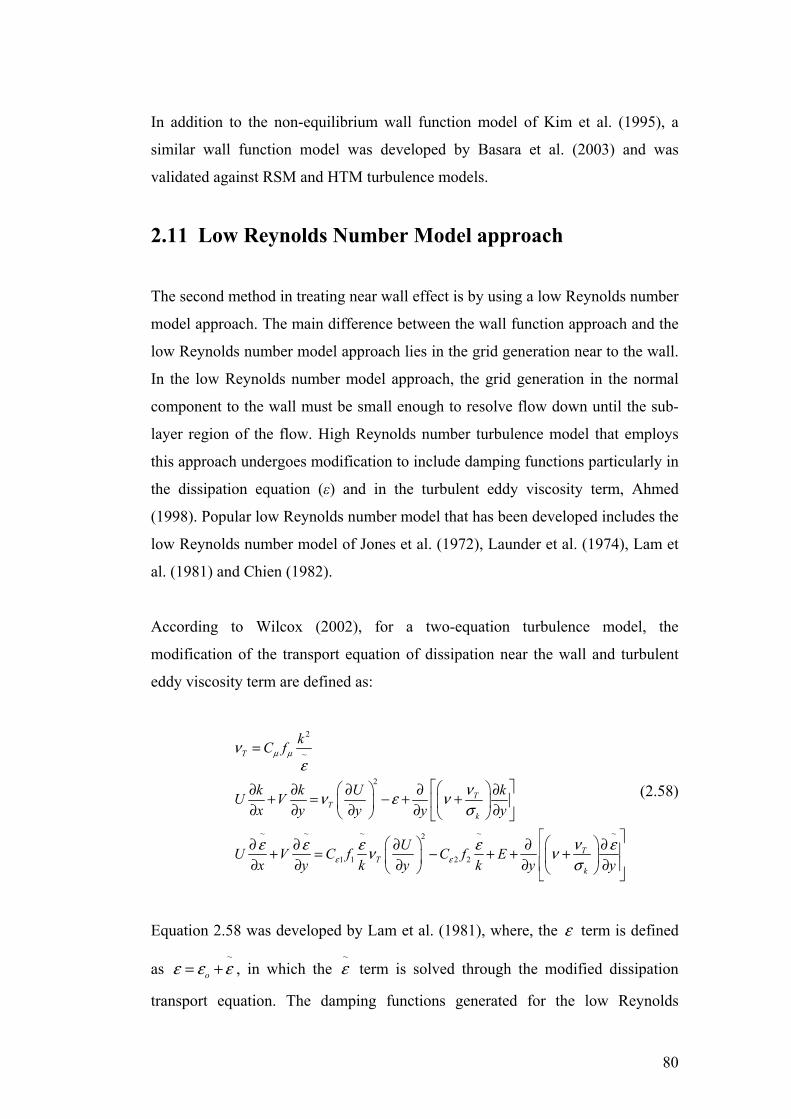
In addition to the non-equilibrium wall function model of Kim et al. (1995), a
similar wall function model was developed by Basara et al. (2003) and was
validated against RSM and HTM turbulence models.
2.11 Low Reynolds Number Model approach
The second method in treating near wall effect is by using a low Reynolds number
model approach. The main difference between the wall function approach and the
low Reynolds number model approach lies in the grid generation near to the wall.
In the low Reynolds number model approach, the grid generation in the normal
component to the wall must be small enough to resolve flow down until the sub-
layer region of the flow. High Reynolds number turbulence model that employs
this approach undergoes modification to include damping functions particularly in
the dissipation equation (ε) and in the turbulent eddy viscosity term, Ahmed
(1998). Popular low Reynolds number model that has been developed includes the
low Reynolds number model of Jones et al. (1972), Launder et al. (1974), Lam et
al. (1981) and Chien (1982).
According to Wilcox (2002), for a two-equation turbulence model, the
modification of the transport equation of dissipation near the wall and turbulent
eddy viscosity term are defined as:
2
~
2
~ ~ ~ ~2
1 1 2 2
T
TT
k
TT
k
kC f
k k U kU Vx y y y y
UU V C f C f E~
x y k y k y
μ μ
ε ε
νε
νν ε νσ
νε ε ε εν νσ
=
⎡ ⎤⎛ ⎞⎛ ⎞∂ ∂ ∂ ∂ ∂+ = − + +⎢ ⎥⎜ ⎟⎜ ⎟∂ ∂ ∂ ∂ ∂⎝ ⎠ ⎝ ⎠⎣ ⎦
yε⎡ ⎤⎛ ⎞⎛ ⎞∂ ∂ ∂ ∂ ∂⎢ ⎥+ = − + + +⎜ ⎟⎜ ⎟∂ ∂ ∂ ∂ ⎢ ∂ ⎥⎝ ⎠ ⎝ ⎠⎣ ⎦
(2.58)
Equation 2.58 was developed by Lam et al. (1981), where, the term is defined
as , in which the term is solved through the modified dissipation
transport equation. The damping functions generated for the low Reynolds
ε~
oε ε ε= +~ε
80

number to take place are given as and E. In addition, as described
previously, the application of the damping function and the low Reynolds number
models are dependent on the turbulence Reynolds number and
1 2, , , of f fμ ε
y+ values near the
wall.
In certain cases, a one-equation model is preferred in the near wall region to
couple with either the high Reynolds number two-equation or RSM turbulence
model. This was due to the fact that the empirical nature of the one-equation
model often provides good prediction for near wall flow. Popular one-equation
model used for near wall model approach include Wolfstein (1969) and Norris et
al. (1975). This kind of approach is also known as the two-layer model approach,
FLUENT (2003), Naser (1990, 2003).
When the low Reynolds number model is used, the switch from the high Reynolds
number turbulence model to the low Reynolds number wall model is normally
done when the turbulent Reynolds number (equation 2.59) is less then 200.
2 1k y k k / 2
ReTlρ
μ νε ν≡ = ≡ (2.59)
To resolve the flow all the way until the viscous sub-layer, the adjacent grid
requirement next to the wall must be y+ < 5 and at least 10 grids generated in the
sub-layer region of Reynolds turbulent number lesser than 200, FLUENT (2003).
For the one-equation of Wolfstein (1967, 1969), the turbulent kinetic energy, k,
equation is and the turbulent eddy viscosity are defined as:
1/ 2
3/ 22 2 2
2 2 2 0
T
T DT
k D
C k l
C kk k uy y y l
μ μμ ρ
μ ρμ μσ
=
∂ ∂ ∂+ + −∂ ∂ ∂
= (2.60)
Where the turbulent and dissipation length scale, lμ and Dl are defined as:
81

( )( )
Re
Re
1
1
T
T
A
AD
l y e
l y e
μ
ε
μ−
−
= −
= − (2.61)
In most cases, the length scale in equation 2.60 has been modified to suit the ones
given by Chen et al. (1988), which is defined as:
( )( )
Re /3/ 4
Re /3/ 4
1
1
T
T
A
AD
l yC e
l yC e
μ
ε
μ μ
μ
κ
κ
−−
−−
= −
= − (2.62)
For the RSM turbulence model, the low Reynolds number flow effect is
incorporated in the modelled dissipation term and also in the pressure strain
redistribution term, Wilcox (2002). Manceau et al. (2002) have introduced an
elliptical blending model to take account of the near wall low Reynolds number
effect. The model was based on the elliptical relaxation model of Durbin (1993)
and is defined as:
( )1 wij ij ijk k hφ α φ αφ= − + (2.63)
Where, hijφ was taken as the pressure strain redistribution model of Speziale et al.
(1991) from equation 2.120 and wijφ is the wall reflection effect defined as:
( )152
wij ik j k jk i k km k m i j ijn n n n n n n n
kεφ τ τ τ⎛ ⎞= − + − −⎜ ⎟⎝ ⎠
δ (2.64)
However, results have shown that although low Reynolds number model for near
wall treatment have managed to reproduce an appropriate C value for the
logarithmic law equation, it still does not manage to predict good results for flow
close to the wall, Wilcox (2002). It was shown in Wilcox (2002) that in most
cases under adverse and favorable pressure gradient application, the low Reynolds
82
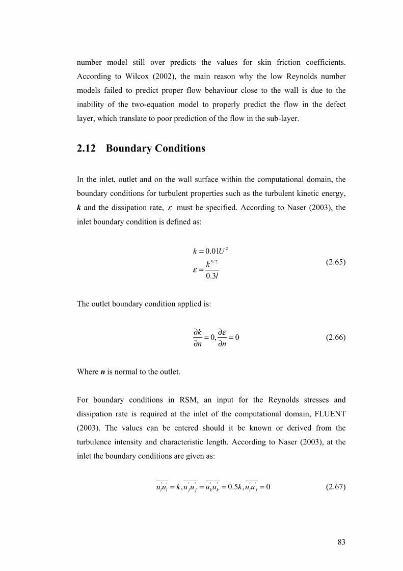
number model still over predicts the values for skin friction coefficients.
According to Wilcox (2002), the main reason why the low Reynolds number
models failed to predict proper flow behaviour close to the wall is due to the
inability of the two-equation model to properly predict the flow in the defect
layer, which translate to poor prediction of the flow in the sub-layer.
2.12 Boundary Conditions
In the inlet, outlet and on the wall surface within the computational domain, the
boundary conditions for turbulent properties such as the turbulent kinetic energy,
k and the dissipation rate, must be specified. According to Naser (2003), the
inlet boundary condition is defined as:
ε
2
3/ 2
0.01
0.3
k Uk
lε
=
= (2.65)
The outlet boundary condition applied is:
0, 0kn n
ε∂ ∂= =∂ ∂
(2.66)
Where n is normal to the outlet.
For boundary conditions in RSM, an input for the Reynolds stresses and
dissipation rate is required at the inlet of the computational domain, FLUENT
(2003). The values can be entered should it be known or derived from the
turbulence intensity and characteristic length. According to Naser (2003), at the
inlet the boundary conditions are given as:
' ' ' ' ' ' ' ', 0.5 ,i i j j k k i ju u k u u u u k u u= = = 0= (2.67)
83

Where, FLUENT (2003), specify the boundary condition value at the inlet as:
' ' ' ' ' '
' ' ' '
0.5 0.5 0.5
2 , 03
i i j j k k
m m i j
u u u u u u k
u u k u u
= =
Σ = =
= (2.68)
For the outlet, the boundary conditions are given as:
( )' '
0i ju un
∂=
∂ (2.69)
According to FLUENT (2003), on the wall surface, the no slip boundary
conditions for k is defined as:
0kn∂ =∂
(2.70)
Where n is the local coordinate normal to the wall. The boundary conditions for
the production of k and is defined as: ε
1/ 4 1/ 2
3/ 4 3/ 2
wk w
P P
P
P
PC k y
C ky
μ
μ
ττκρ
εκ
≈
= (2.71)
At the wall, FLUENT (2003) obtained near wall valued of Reynolds stresses and
dissipation rate from the wall function. By this, FLUENT assumes turbulence to
be in equilibrium. The Reynolds stresses are then computed from:
'2 ' ''2 '2
1.098, 0.247, 0.655, 0.255u uu u
k k k kητ λ= = = − =
uτ η (2.72)
84
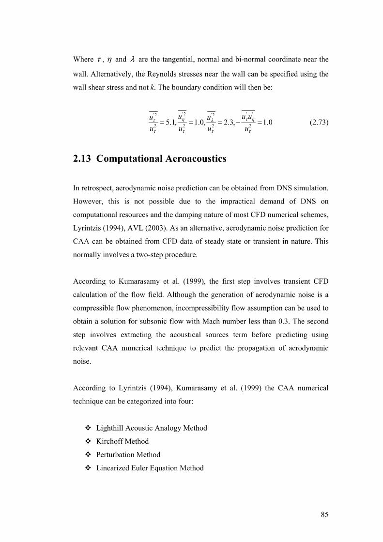
Where , τ η and λ are the tangential, normal and bi-normal coordinate near the
wall. Alternatively, the Reynolds stresses near the wall can be specified using the
wall shear stress and not k. The boundary condition will then be:
'2 ' ''2 '2
2 2 2 25.1, 1.0, 2.3, 1.0u uu u
u u u uη ττ λ
τ τ τ τ
= = = − =uη (2.73)
2.13 Computational Aeroacoustics
In retrospect, aerodynamic noise prediction can be obtained from DNS simulation.
However, this is not possible due to the impractical demand of DNS on
computational resources and the damping nature of most CFD numerical schemes,
Lyrintzis (1994), AVL (2003). As an alternative, aerodynamic noise prediction for
CAA can be obtained from CFD data of steady state or transient in nature. This
normally involves a two-step procedure.
According to Kumarasamy et al. (1999), the first step involves transient CFD
calculation of the flow field. Although the generation of aerodynamic noise is a
compressible flow phenomenon, incompressibility flow assumption can be used to
obtain a solution for subsonic flow with Mach number less than 0.3. The second
step involves extracting the acoustical sources term before predicting using
relevant CAA numerical technique to predict the propagation of aerodynamic
noise.
According to Lyrintzis (1994), Kumarasamy et al. (1999) the CAA numerical
technique can be categorized into four:
Lighthill Acoustic Analogy Method
Kirchoff Method
Perturbation Method
Linearized Euler Equation Method
85

2.14 Lighthill Acoustic Analogy Method
Majority of study on CAA incorporate the Lighthill Acoustic Analogy to evaluate
for aerodynamic noise propagation. The Lighthill Acoustic Analogy was made
famous by the late Professor Sir James Lighthill where in 1951 and 1954
introduced papers proposing a theory on aerodynamic noise generation in free
stream flow, Goldstein (1976). In a review made by Firoz (2000), Lighthill
postulated that all non-linearities in a fluctuating hydrodynamic flow of a large
volume of fluid act as sources of sound. The source of aerodynamic noise is given
by the Lighthill stress tensor, which is derived thorough the manipulation of the
continuity and momentum equation to form an in homogeneous wave equation.
This set of formulation is famously known as the Lighthill’s acoustic analogy. In
addition, through dimensional analysis, Lighthill’ acoustic analogy have shown to
provide a quadrupole type sound source distribution, AVL (2003).
According to Goldstein (1976), the Lighthill’s acoustic analogy equation is
defined as:
2'
2
,1
4
ijo
vo i j
x yT y t
ady
a x x x yρ
π
⎛ − ⎞−⎜ ⎟
∂ ⎝ ⎠=∂ ∂ −∫ (2.74)
with is the Lighthill’s turbulence stress tensor and is defined as: ijT
( ) ( )2ij o i j ij o o o ijT v v p p cρ δ ρ ρ⎡= + − − − −⎣ e⎤⎦ (2.75)
According to Goldstein (1976), in order to solve for the Lighthill’s acoustic
analogy equation, the sound source term, which is the Lighthill’s stress tensor
( ) must be known. However, to obtain a solution for is virtually impossible
for most flows of interest since it is equivalent to solving the complete non-linear
ijT ijT
86
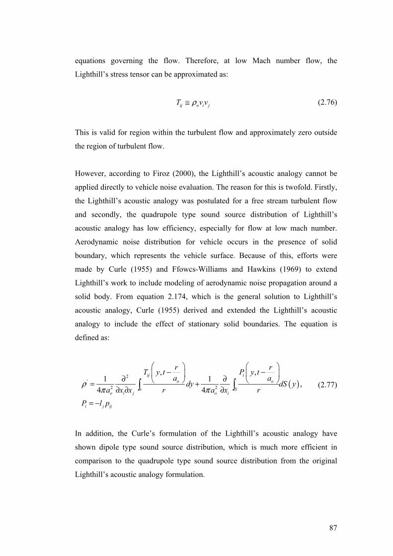
equations governing the flow. Therefore, at low Mach number flow, the
Lighthill’s stress tensor can be approximated as:
ij o i jT v vρ≅ (2.76)
This is valid for region within the turbulent flow and approximately zero outside
the region of turbulent flow.
However, according to Firoz (2000), the Lighthill’s acoustic analogy cannot be
applied directly to vehicle noise evaluation. The reason for this is twofold. Firstly,
the Lighthill’s acoustic analogy was postulated for a free stream turbulent flow
and secondly, the quadrupole type sound source distribution of Lighthill’s
acoustic analogy has low efficiency, especially for flow at low mach number.
Aerodynamic noise distribution for vehicle occurs in the presence of solid
boundary, which represents the vehicle surface. Because of this, efforts were
made by Curle (1955) and Ffowcs-Williams and Hawkins (1969) to extend
Lighthill’s work to include modeling of aerodynamic noise propagation around a
solid body. From equation 2.174, which is the general solution to Lighthill’s
acoustic analogy, Curle (1955) derived and extended the Lighthill’s acoustic
analogy to include the effect of stationary solid boundaries. The equation is
defined as:
( )2
'2 2
, ,1 1 ,
4 4
ij io o
v So i j o i
i j ij
r rT y t P y ta a
dy dS ya x x r a x r
P l p
ρπ π
⎛ ⎞ ⎛ ⎞− −⎜ ⎟ ⎜ ⎟∂ ∂⎝ ⎠ ⎝ ⎠= +
∂ ∂ ∂
= −
∫ ∫ (2.77)
In addition, the Curle’s formulation of the Lighthill’s acoustic analogy have
shown dipole type sound source distribution, which is much more efficient in
comparison to the quadrupole type sound source distribution from the original
Lighthill’s acoustic analogy formulation.
87

Ffowcs-Williams and Hawkins (1969) have also extended Curle’s-Lighthill’s
formulation to include flow for moving solid boundaries, for example in flow
involving helicopter rotors. According to Kumarasamy et al. (1999), the Ffowcs-
Williams and Hawkins formulation is appropriate for high-speed flow
applications. For low Mach number flows, the simpler Curle’s-Lighthill’s
formulation is recommended for use.
Other notable contributors to the extension of Lighthill’s acoustic analogy for
various aerodynamic noise applications include Powell (1964), Howe (1975,
1981, 1993) and Jenvey (1989). Powell’s (1964) contribution involved work on
the generation of aerodynamic noise from unsteady vortex flow. On the other
hand, Howe (1975, 1981, 1993) was involved in the study of aerodynamic noise
generation from turbulent separated flows, especially trailing edge flow. Finally,
Jenvey (1989) contributed in the development areas of mean sound power
formulation from time-stationary motion.
2.15 Kirchoff Method
According to Kumarasamy et al. (1999), the Kirchoff method separates the
computational domain into an inner and outer region. The inner is a non-linear
region close to the sources and is solved using a CFD solver. The outer is a linear
region and is solved using an integral equation for sound pressure level base on
the sources distributed on the surface edge of inner region (defined as Kirchoff
surface), which can be either stationary or non-stationary. More information on
Kirchoff method is available in from Lyrintzis (1994).
2.16 Perturbation Method
According to Bergamini et al. (1997), the perturbation method solves the
incompressible and acoustic parts of the flow, using two different grids, thus
reducing overall computational time. In predicting aerodynamic noise
propagation, the difference between the acoustic and the incompressible quantities
88

are taken as the source terms and solved using an Euler type of equation. More
information on the perturbation method is available from Hardin (1995).
2.17 Linearized Euler Equation Method
The CAA prediction technique using Linearised Euler equation method originally
uses nonlinear/unsteady CFD calculation to predict near-field acoustic source
term (Lighthill’s stress tensor, ) and uses the linearised Euler equation to
predict the far-field aerodynamic noise propagation, Lyrintzis (1994). However,
according to AVL (2003), in using non-linear CFD approach to determine , a
high computational effort is required, in terms of both memory and storage
capacity. Furthermore, according to Lele (1997), formulation will breakdown
whenever significant refractive effects are present in the flow. In addition, a
tailored Green’s function needs to be developed for different geometry to take
account of diffraction effect from interaction between the flow and solid
boundaries.
ijT
ijT
To overcome the requirement of using non-linear CFD approach to determine ,
an alternative approach was developed by Bechera (1996), where he used models
based on the space-time correlation function of the turbulent velocity fluctuations.
In his model, Bechera (1996) uses eddy length scale, decay rate and turbulent
kinetic energy data obtained from a steady RANS computation to determine for
. Lighthill acoustic analogy is then used to develop a relationship between the
near field and far-field noise correlation, AVL (2003).
ijT
ijT
Longatte then extended the approach of Bechera (1996) by using a statistical
model formulation instead of using the Lighthill’ acoustic analogy to forge a
relation between the near-field and far-field aerodynamic noise. The approach by
Bechera (1996) is still used to determine a time accurate formulation using the
space-time correlation model with data for acoustic source terms estimation
obtained from steady CFD RANS results. The aerodynamic noise propagation
89

from the source to the receiver is then modeled using a linearized Euler equation.
In addition, refraction and diffraction effects are handled automatically by the
linearised Euler equation, AVL (2003).
AVL SWIFT CAA (2003) uses the CAA prediction technique with linearised
Euler equation developed by Bechera (1996) and Longatte (1998. This technique
employed by AVL SWIFT CAA is a hybrid approach where two separate grids
and also calculations are needed for the CFD and CAA prediction. Furthermore,
according to AVL (2003), unstructured grid is used for the CAA prediction, which
allows for handling arbitrarily complex geometries. In addition, the CAA
prediction approach employed by AVL SWIFT is aimed at predicting the
broadband noise and cannot be used to predict tonal or periodic noise.
The steps involve in the calculation of CAA in SWIFT is broken down into three,
which is:
Time –averaged CFD simulation with RANS solver
Acoustic Source Generation
Acoustic loads-radiated noise with unstructured Linearized Euler Solver
In the first step, the CFD simulation is carried out to determine both the mean
flow and turbulence statistics. The mean flow is to be used in step two and three.
The turbulence statistics are used to determine the acoustics sources in step two.
In the second step, the acoustic sources are estimated from the turbulent
fluctuations. In the third step, the propagation of the aerodynamic noise is
calculated through the use of the linearised Euler equations through the use of
Discontinuous Galerkin Method, AVL (2003).
Once the steady RANS CFD simulation have been conducted, the SWFT CAA
determined the acoustic sources from the governing equations of mass,
momentum and energy. These equations of mass, momentum and energy are
defined as follows:
90

Mass
. mU Stρ ρ∂ +∇ =∂
(2.78)
Momentum
. IU UU p Stρ ρ∂ +∇ +∇ =∂
(2.79)
Energy
( ) ( )
( ) ( ) ( )
2
1
1. 1
21 . . .
E
E
p U p S U St
U S p U Q p U
γγ
γ γ γ
−∂ + ∇ = − +∂− − − ∇ = − ∇
M (2.80)
Similar to the generation of the Lighthill’s equations, the mass equation was
multiplied by U and subtracted from the momentum equation to obtain:
( ) ( ) ( )1 1. I M IU U U S p US Q pt ρ ρ
∂ + ∇ = −∇ − = −∇∂
(2.81)
According to AVL (2003), the mass, momentum and energy equations generated
five unknowns, which was density, ρ , the three components of velocity, U and
pressure, p . These unknowns are solved using the Linearised Euler Equations
(LEE).
The first step in using LEE to solve for density, velocity and pressure was to first
divide them into free stream and acoustics components. For velocity, a turbulent
component was also included.
Density o aρ ρ ρ= + (2.82)
Pressure o ap p p= + (2.83)
Velocity o aU U u u= + + t (2.84)
91
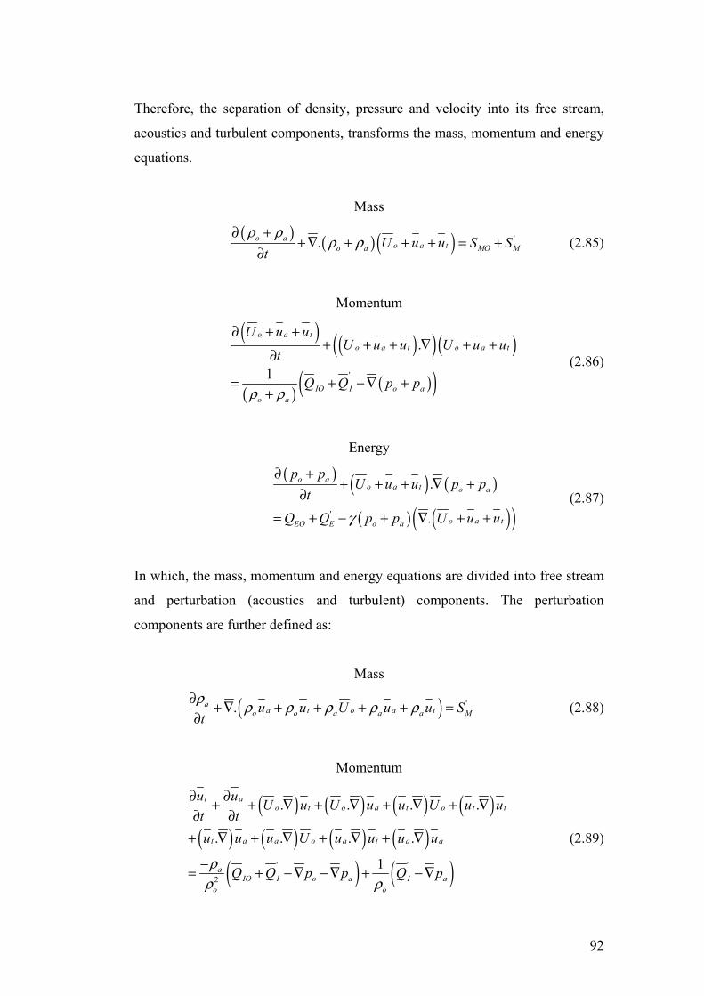
Therefore, the separation of density, pressure and velocity into its free stream,
acoustics and turbulent components, transforms the mass, momentum and energy
equations.
Mass
( ) ( )( ) '.o ao a to a MOU u u S S
tρ ρ
ρ ρ∂ +
+∇ + + + = +∂ M (2.85)
Momentum
( ) ( )( )( )
( ) ( )( )'
.
1
o a to a t o a t
o aIO Io a
U u uU u u U u u
t
Q Q p pρ ρ
∂ + ++ + + ∇ + +
∂
= + −∇ ++
(2.86)
Energy
( ) ( ) ( )
( ) ( )( )'
.
.
o ao a t o a
o a tEO E o a
p pU u u p p
tQ Q p p U u uγ
∂ ++ + + ∇ +
∂
= + − + ∇ + + (2.87)
In which, the mass, momentum and energy equations are divided into free stream
and perturbation (acoustics and turbulent) components. The perturbation
components are further defined as:
Mass
( ) '.aa t o a to o a a au u U u u S
t Mρ ρ ρ ρ ρ ρ∂ +∇ + + + + =∂
(2.88)
Momentum
( ) ( ) ( ) ( )( ) ( ) ( ) ( )
( ) ( )' '
2
. . . .
. . . .
1
t ao t o a t o t
t a a o a t a a
ao a aIO I I
o o
u u U u U u u U u ut tu u u U u u u u
Q Q p p Q pρρ ρ
∂ ∂+ + ∇ + ∇ + ∇ + ∇∂ ∂+ ∇ + ∇ + ∇ + ∇
−= + −∇ −∇ + −∇
t
(2.89)
92

Energy
( )
( ) ( ) ( ) ( ) ( )'
. . . . .
. . . .
ao a a t ta o a o a
o a t aE a a a o o
pU p u p u p u p u p
tQ p U p u p u p u p uγ γ γ γ γ
∂+ ∇ + ∇ + ∇ + ∇ + ∇ =
∂− ∇ − ∇ − ∇ − ∇ − ∇. t
(2.90)
Furthermore, according to AVL (2003), the second order and cross terms in the
perturbation equations are neglected to further simplify the set of equations.
Mass
( ) '.aa oo a M ou U S
t. tuρ ρ ρ ρ∂ +∇ + = −∇
∂ (2.91)
Momentum
( ) ( ) ( ) ( )( ) ( ) ( )
'
2
1. .
. . .
a ao a a o o aIO I
o o
to t t o t t
u U u u U Q p Q pt
u U u u U u ut
ρρ ρ−∂ + ∇ + ∇ = −∇ + −∇
∂
∂− − ∇ − ∇ − ∇∂
(2.92)
Energy
( ) ( ) ( ) ( )'. 1 . 1ao a a o ta o E o a
pU p u p Q u p p U u p
tγ γ γ
∂+∇ + = + − ∇ − − ∇ − ∇
∂. . o (2.93)
From the simplified equations of mass, momentum and energy, the left hand side
of these equations is solved from the LEE of acoustic density, velocity and
pressure respectively. The right hand side of these equations contains sets of
source terms. The aerodynamic source generation for mass, momentum and
energy are defined as:
93

Mass
( )1 . . .t t t to o oS u u u u . oρ ρ ρ ρ= −∇ = − ∇ + ∇ = − ∇ (2.94)
Momentum
( ) ( ) ( )2 . . .o t t o tS U u u U u= − ∇ − ∇ − ∇ tu (2.95)
Energy
5 .t oS u p= − ∇ (2.96)
The aerodynamic noise source generation are required as part of the input in the
acoustic propagation module. It can be seen that in order to solve for the
aerodynamic source generation, the turbulent velocity fluctuation term needs to be
determined. This is done through reconstruction of the turbulent quantities from
the solved steady RANS CFD simulation.
According to AVL (2003), the turbulent velocity can be obtained through the
inverse Fourier transform process and can be defined as:
( ) ( )~
12 cos .
N
n n nn
u x u xκ nψ σ=
= +∑ (2.97)
Where, nψ , is a random phase, , is the wave-vector and , is the direction of
the turbulent velocity vector, which is perpendicular to . is the mode
amplitude and is defined as:
nκ nσ
nκ~
nu
( )~
nu E dκ κ= n (2.98)
( )E κ is the distribution of energy over the wave numbers and is further defined
as:
94

( )2
2
4
2
17 / 62
231.453
1
e
e
e
kE ν
κκ
κκ
κκ κ
κ
⎛ ⎞−⎜ ⎟⎜ ⎟⎝ ⎠
⎛ ⎞⎜ ⎟⎝ ⎠=
⎛ ⎞⎛ ⎞⎜ ⎟+ ⎜ ⎟⎜ ⎟⎝ ⎠⎝ ⎠
e (2.99)
Where, , is the turbulent kinetic energy obtained from the CFD RANS results.
, is the peak wave number over the selected wave-number spectrum and
k
eκ νκ is
the Kolmogorov wave number. Both and eκ νκ are defined as:
0.747eκ =
Λ (2.100)
and
43νεκν
= (2.101)
Where, the dissipation rate, is determined from the RANS CFD results and the
turbulent integral length scale, is defined as:
ε
Λ
( )3/ 22 / 3fac
kε
Λ = Λ (2.102)
The time dependent domain for turbulent velocity is determined from similar
relationship as equation 2.180 using inverse Fourier transforms with a time
dependent phase and is defined as:
( ) ( ) ( )
( )( )
~
1~
1
, 2 cos . ,
2 cos .
Nn n n n nn
Nn n n nn
u x t u x t u x t
u x Ut
κ ψ ω σ
κ ψ σ
=
=
= + +
= − +
∑∑
= (2.103)
95

Where, the radial frequency, is defined as: nω
.n n Uω κ= − (2.104)
In addition, the coupling between spatial and time domain modifies the energy
distribution relationship and is defined as:
( ) ( ) ( ) ( ) ( ) ( )( 2~ 0.5 /1,2
n o oa
n n n m n o no
E E E ea
ω ω ωκ ω κ φ ω ω κ
ω π)⎡ ⎤− −⎢ ⎥⎣ ⎦= − = (2.105)
Once the aerodynamic noise source generation has been determined, the final
acoustic propagation module is then obtained by using LEE in three-dimensional
conversation form.
( ) ( )jj
L U U F U St x∂ ∂= + =∂ ∂
(2.106)
Where, the perturbation components, , , , ,U u v w pρ= is described, with respect to
the mean flow. The LEE equation is solved using a method called the Quadrature-
Free Discontinuous Galerkin spatial discretization approach in which, further
references can be obtained from Atkins and Shu (1998). In this method, the LEE
equation is multiplied by a weighting function, W, and integrated over a finite-
dimensional subspace. Thus, the equation is further refined to:
( )Th h hW L U d W Sd
Ω Ω
Ω = Ω∫ ∫ T
x
(2.107)
Where, and are defined as: hU hW
( ) ( ), ,1 0
eN M
h i k i ki k
U v t b= =
=∑∑ (2.108)
96

( ), ,1 0
eN M
h i k i ki k
W w b= =
=∑∑ x (2.109)
And is the base function, which is further defined as: ,i kb
( ), ,
i i
i k h i kb L U d b SdΩ Ω
Ω = Ω∫ ∫ (2.110)
In order for the base function, to be second order accurate, the equation is
modified using Gauss’ theorem and thus written as:
,i kb
( ) ( ),, ,
i i i i
i khi k i k j h j j h i k
j
bUb d b F U n d F U d b Sdt xΩ Γ Ω Ω
∂∂ Ω+ Γ − Ω = Ω∂ ∂∫ ∫ ∫ ∫ , (2.111)
Where, in order to become Quadrature-free, S, is defined as:
( ) ( )3
, ,1 0
eN
h i k i ki k
S S S t b x= =
≈ =∑∑ (2.112)
97

Chapter Three
METHODOLOGY
This chapter describes the methodology for this project. This chapter discuss the
general CFD approach and the accuracy associated with it. This is followed by
discussion of grid generation techniques, discretization and numerical schemes.
This chapter also discusses the near wall model and turbulence models available.
Lastly, this chapter describes the CAD model and input boundary conditions used
in this project.
3.1 General CFD Approach Process
There are three steps involved in a typical CFD simulation. The three steps are:
• Pre-Processing Stage
• CFD Solving Stage
• Post-Processing Stage
In the pre-processing stage, CFD users are needed to provide sufficient input to
the computer in order to obtain the desired output. The pre-processing stage is
divided into several steps:
• Geometry Generation
• Mesh Generation
• Input for Boundary Condition
• Flow Type (Steady/Unsteady)
• Discretization Scheme Input
• Turbulence and Near Wall Model Input
The second stage is the solving stage where the physics of the flow is being
solved by the computer. The third and final stage is called the post-processing
98

stage where analysis of graphical representation of the numerical results takes
place.
3.2 Accuracy Factors and Errors Associated with CFD
As discussed in previous sections, the limitations of computational performance
are hindering CFD in reaching its full potential. Due to these limitations,
numerical models are always developed to solve for flow and this leads to
assumptions and approximations being made by researchers. According to Naser
(1990), numerical models are categorised into two types: the Phenomenological
and Multi-dimensional models. Multi-dimensional models are more accurate and
extensive since it models both spatial and temporal information of the flow.
However, Phenomenological models are much more cost effective since it models
only the temporal part of the flow. In general, these numerical models are
subjected to solution errors that will affect the accuracy of the CFD results.
Numerical solution from CFD has approximately 10 to 15% error comparison to
empirical results, Swinburne (2000). The causes of solution errors in a CFD
simulation are:
• Error due to Discretization
• Equation solver/Round-off Error
According to Anderson (1995), discretization error is defined as the difference
between the exact analytical solutions based on the governing partial differential
equation of flow (continuity equation, Navier-Stokes equation together with
Turbulence Model that is chosen and Energy equation) and the algebraic
equations developed from corresponding numerical scheme. In the discretizing
process, the governing partial differential equations is transformed into systems of
algebraic equations via numerical scheme, truncation errors (round-off of
numerical scheme) are being introduced. Furthermore, the discretization process
requires numerical treatment of boundary conditions to take place and this induces
99

additional errors as well. In addition, the accuracy of the discretization process
relies on the grid refinement and quality of the computational domain.
High grids generation and refinement in a given CFD flow domain that results in
low discretization error will provide better simulation of the flow physics through
better visualization in the post-processing stage. This is especially true for areas
within the flow that is subjected to high change in pressure gradients. However,
the resulting computation time will take much longer. The refinement procedure is
called the grid-independency procedure. In the grid-independency procedure,
converged numerical solution is then refined, usually by doubling its density. The
flow is then solved again. The grid-independency procedure is stopped once the
difference in numerical solution between grid refinements is small, normally
within 5.0% of each other. However, it is also important to establish smoothness
around the grid refinement areas. Large variations in grid shape or density can
cause numerical diffusion, resulting in inaccurate results or simulation instability.
In addition, high grid quality also needs to be maintained within the
computational domain. There are two factors that determine grid quality. They
are:
• Aspect Ratio
• Grid Skewness (Distortion)
Grid aspect ratio is given by the ratio of the length and width (∆y/∆x) of any given
grid surface. The ideal aspect ratio is 1.0, with the minimum requirement
normally to either be larger than 0.2 or smaller than 5.0, Swinburne (2000). A
poor grid aspect ratio will normally lead to poor accuracy in numerical results and
a possibility of divergence during solver iterations.
Grid skewness is given by the angle of skewness between two edges on a given
grid. The most ideal grid skewness is θ=90°, Swinburne (2000). However,
minimum requirement in grid skewness is to be maintained in between 45° and
135°. Poor grid skewness can also lead to low level of accuracy of numerical
results and divergence during solver iterations.
100

According to Anderson (1995), equation solver/round-off error is caused during
the solving stage. In the solving stage, iteration process takes place where
repetitive calculations are done in order to achieve a numerical solution. The
iteration process often “round-off” calculated numbers into significant figures,
resulting in error. The iteration process is repeated until the solution converged.
Convergence is a limit set by the CFD user to stop the iteration process once the
difference between calculated values of the iteration results is too small. Normally
convergence limit are set when differences in iteration results are to within 0.1%
of each other.
It has been discussed in this section the importance of grid generation and
discretization scheme in determining the accuracy of numerical results in CFD
simulations. In the next sections, more detailed discussion will be presented on
grid generation and discretization schemes in CFD especially on automotive type
problem. Discussion will cover various types and implementation strategies used
on grid generation and discretization scheme.
3.3 CFD Grid Generation and Discretization Methods
In order to generate the highest quality of grids for the highest level of accuracy
on a CFD simulation, grids generated depends on the complexity of the flow
problem. For high complex flow problems, a more complex high quality grids
need to be generated for the CFD simulation. This high level of flow complexity
applies for automotive type problems. However, the applications of complex grid
generation in automotive flow problems are dependent on the overall performance
of the modern day computers. Before high performance computers were
developed, a lot of simplifications were made on the governing mathematical
equations of the flow. This reduces the complexity of the grids generated for the
CFD simulation. The generations of grids and employing of discretization
schemes for a simplified flow were done using a Linear or Potential flow method.
After the development of supercomputers that are capable in handling complex
101
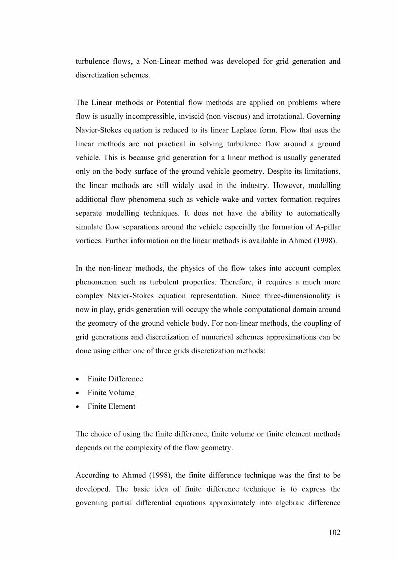
turbulence flows, a Non-Linear method was developed for grid generation and
discretization schemes.
The Linear methods or Potential flow methods are applied on problems where
flow is usually incompressible, inviscid (non-viscous) and irrotational. Governing
Navier-Stokes equation is reduced to its linear Laplace form. Flow that uses the
linear methods are not practical in solving turbulence flow around a ground
vehicle. This is because grid generation for a linear method is usually generated
only on the body surface of the ground vehicle geometry. Despite its limitations,
the linear methods are still widely used in the industry. However, modelling
additional flow phenomena such as vehicle wake and vortex formation requires
separate modelling techniques. It does not have the ability to automatically
simulate flow separations around the vehicle especially the formation of A-pillar
vortices. Further information on the linear methods is available in Ahmed (1998).
In the non-linear methods, the physics of the flow takes into account complex
phenomenon such as turbulent properties. Therefore, it requires a much more
complex Navier-Stokes equation representation. Since three-dimensionality is
now in play, grids generation will occupy the whole computational domain around
the geometry of the ground vehicle body. For non-linear methods, the coupling of
grid generations and discretization of numerical schemes approximations can be
done using either one of three grids discretization methods:
• Finite Difference
• Finite Volume
• Finite Element
The choice of using the finite difference, finite volume or finite element methods
depends on the complexity of the flow geometry.
According to Ahmed (1998), the finite difference technique was the first to be
developed. The basic idea of finite difference technique is to express the
governing partial differential equations approximately into algebraic difference
102

equations form using finite difference schemes at the grid nodal points. Finite
difference methods often employ curvilinear orthogonal grid system that it is
difficult and time consuming to generate especially in three-dimensional
computational domain. This results in governing transport equations that has more
terms. This difficulty makes the finite difference techniques seldom used in
automotive CFD.
In the finite volume methods, the computational domain is split up into many
small control volumes. The partial differential governing equations are integrated
over each of the control volumes and the resulting integrated governing equations
are then discretized using finite-difference schemes. A resulting set of algebraic
equations is then formed, which are then solved. The main advantage of finite
volume methods over the finite difference methods is that the finite volume
methods can use both structured orthogonal and non-orthogonal grid system. In
the non-orthogonal grid system, irregular unstructured grids can be used. As a
result, various grid shapes and size can be used for the finite volume methods.
This is however, at the expense of additional computational resource. Because of
the flexibility in grid generation of the finite volume methods, it is the most
preferable methods used in automobile aerodynamics applications.
In the finite element methods, the computational domain is split up into small
volumes, called elements. Within each element, values are being approximated as
a linear combination of weighting residuals and use the integral form of the
governing differential equations for each element volume without direct reference
to other cells. Information is shared among all the other grid points in the element.
This method generally uses irregular unstructured grid, often in a triangular
shaped element. By employing irregular unstructured grids, the treatment of
complex surface geometry is possible and furthermore, it also allows local grid
refinements at critical areas without the penalty of simultaneous grid refinements
at other areas. However, this also serves as a disadvantage since sufficient refined
grids in finite element methods are needed to give solution of high accuracy, Du
Pont (2001).
103
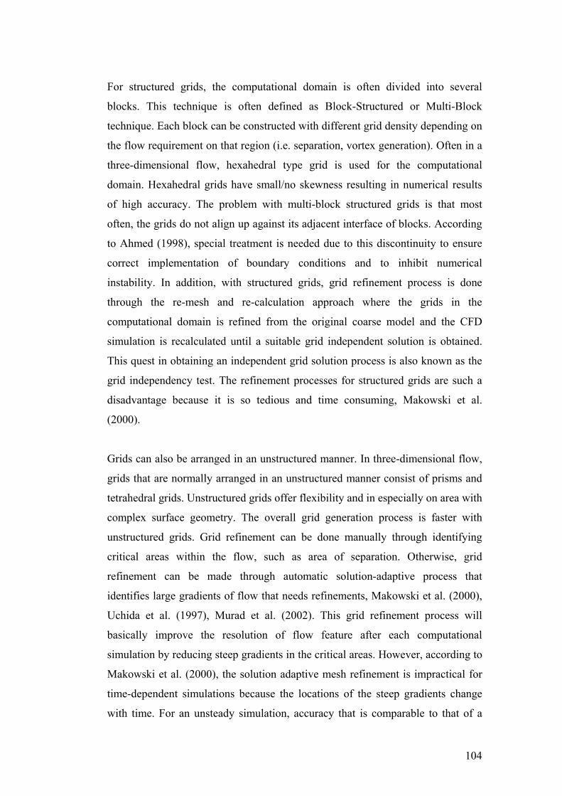
For structured grids, the computational domain is often divided into several
blocks. This technique is often defined as Block-Structured or Multi-Block
technique. Each block can be constructed with different grid density depending on
the flow requirement on that region (i.e. separation, vortex generation). Often in a
three-dimensional flow, hexahedral type grid is used for the computational
domain. Hexahedral grids have small/no skewness resulting in numerical results
of high accuracy. The problem with multi-block structured grids is that most
often, the grids do not align up against its adjacent interface of blocks. According
to Ahmed (1998), special treatment is needed due to this discontinuity to ensure
correct implementation of boundary conditions and to inhibit numerical
instability. In addition, with structured grids, grid refinement process is done
through the re-mesh and re-calculation approach where the grids in the
computational domain is refined from the original coarse model and the CFD
simulation is recalculated until a suitable grid independent solution is obtained.
This quest in obtaining an independent grid solution process is also known as the
grid independency test. The refinement processes for structured grids are such a
disadvantage because it is so tedious and time consuming, Makowski et al.
(2000).
Grids can also be arranged in an unstructured manner. In three-dimensional flow,
grids that are normally arranged in an unstructured manner consist of prisms and
tetrahedral grids. Unstructured grids offer flexibility and in especially on area with
complex surface geometry. The overall grid generation process is faster with
unstructured grids. Grid refinement can be done manually through identifying
critical areas within the flow, such as area of separation. Otherwise, grid
refinement can be made through automatic solution-adaptive process that
identifies large gradients of flow that needs refinements, Makowski et al. (2000),
Uchida et al. (1997), Murad et al. (2002). This grid refinement process will
basically improve the resolution of flow feature after each computational
simulation by reducing steep gradients in the critical areas. However, according to
Makowski et al. (2000), the solution adaptive mesh refinement is impractical for
time-dependent simulations because the locations of the steep gradients change
with time. For an unsteady simulation, accuracy that is comparable to that of a
104

well-adapted steady simulation can only be achieved at a much greater total grid
count. In addition, solution adaptive mesh refinement is also useful for
eliminating oscillatory solution resulted from coarse volume mesh, during a
steady flow calculation. However, unstructured grids can sometimes have high
value of skewness, reducing the grid quality. This will reduce the accuracy of the
numerical results.
Apart from using a blend of prism and tetrahedral grids, a more advance grid
generation system called the Arbitrary Cell Technology (ACT) has been
developed. A blend of polyhedral unstructured grids is used to mesh and refine
complex three-dimensional computational domain. The mesh generation
procedure was automatic with very little time consuming manual efforts required.
The advantage of ACT is that grids generation, refinement and manipulation can
be done with extremely ease while retaining the smoothness of the complex
geometry in the computational domain. However, grid refinement process is done
through the same process as structured grids by using the remesh and
recalculation approach each time a new refinement is needed.
A combination of hexahedral/tetrahedral hybrid grids can also be used in the
computational domain (Murad, 2004). Flow close to the vehicle body can be
treated with structured highly accurate hexahedral mesh and free stream flow far
away from the body can be treated using unstructured tetrahedral mesh. Flow
treated using structured hexahedral mesh was done using multi-block method. The
major setback to this technique is that it takes a long time to generate. Grid
refinement process is also hard to do since grid refinement process through
solution adaptive process will upset the whole balance of the generated grids
structure. This technique is used in a computational domain where a final adapted
grid count and grid refinement location has been established.
In order to estimate the size of the time step require to solve for a given grid
interval, the Courant number relationship can be used. The Courant number, Cr is
defined as:
105

v tCrxΔ=Δ
(3.1)
which is the ratio between the product of flow velocity and time step and grid
interval.
3.4 CFD Numerical Schemes
Apart from grid generation, the choice of numerical or interpolation scheme in
discretization methods implementation are important to ensure numerical solution
of high accuracy in order to limit discretization error. Once the computational
domain has been meshed, a set of procedure takes place in discretizing the
governing equations of flow into its linear algebraic form. In CFD, this procedure
is called the discretization or numerical methods. The discretization of governing
equations can be done two ways, either by using a segregated or a coupled solver.
This section discusses the difference between two solvers. In addition, numerical
schemes used to discretize each equation are also discuss together with the
problems associated with each numerical scheme and the treatment used to
overcome the problems.
A good numerical scheme should be able to provide fast convergence of the
iterative solution. This can be achieved by having a numerical scheme that is
stable and consistent. The numerical scheme is said to be stable by being bounded
during the iteration process (does not diverge and oscillate). Consistency of the
numerical scheme is achieved through the ability of obtaining the real solution
(reduction of the truncation error) through grid independency test. The factor that
determines the suitability of various numerical schemes on a particular problem is
the Peclet number. The Peclet number is defined as:
DFxu
ceonducDiffusionCStregthConvectionerPecletNumb =
Γ== δρ
tan (3.2)
106

For discretization of the momentum equation, the most basic numerical scheme
that can be used is the central difference scheme. The central difference scheme is
a higher order scheme. However, the central difference scheme can lead to
unrealistic results especially for Peclet number that is higher than 2. According to
AVL (2003), central difference scheme can generate numerical oscillations
yielding unbounded and non-monotonic solutions. The central difference scheme
is used for low Reynolds number flow. For flow with low Peclet number, the
central differencing scheme is recommended.
For flow with high Peclet number an alternative substitution to the central
difference scheme is to use the upwind scheme. A standard upwind scheme is a
lower order scheme. In the upwind scheme, the value of velocity for the
momentum at the control volume interface is taken as equal to the value of the
grid point on the upstream side of the interface (Patankar, 1980). However,
according to Patankar, at very high Peclet number, the upwind numerical scheme
will yield results that lead to false diffusion. False diffusion will occur for
multidimensional problem especially with flow that is not aligned with the grids.
A remedy recommended by Patankar is to use refined grids at area that produce
false diffusion. A higher order upwind scheme or its modified version (QUICK
numerical scheme) can also be used to reduce false diffusion by taking into
account multidimensional problem (Fluent, 2003, Swinburne, 2000). However,
the QUICK scheme is suited mostly for problems generated using structured
grids.
Apart from the central differencing and upwind scheme, standard numerical
scheme that are available on most CFD software are exponential scheme, hybrid
scheme and power law scheme. Although this numerical scheme does not still
solve the problem of false diffusion, the development and appreciation of such
schemes are still worth discussing. The exponential scheme is developed from the
exact solution of the convection-diffusion term. From the exact solution, it was
discovered that the Peclet number behaves exponentially especially at large
values. This led to the false diffusion problem encountered in the lower order
upwind scheme. The exact solution solved this problem by making the coefficient
107

of the linear discretized equation to match the exponential behaviour. However,
the shortcoming of the exponential scheme is that it is expensive to compute and
still does not provide an accurate solution for multidimensional problem. This led
to the development of the hybrid and Power Law Scheme. Both of these schemes
are of lower order. The hybrid scheme improves the exponential scheme by
making it more economical to use. This was implemented by using the central
differencing scheme at Peclet number between 2.0 and –2.0. At Peclet number
higher than 2.0 or lower than –2.0, the upwind scheme is used. The Power-Law
scheme further refine the hybrid scheme to make it more accurate without
sacrificing much computational resource by combining the exponential and the
upwind scheme. The concept is similar to the hybrid scheme.
In addition, AVL (2003) introduces two higher numerical schemes based on the
‘Total Variation Diminishing Concept (TVD)’ and the ‘Convection Boundedness
Criterion (CBC)’ of Sweby (1984) and Gaskell et al. (1988). These higher order
numerical schemes are known as the MINMOD and SMART schemes
respectively. The MINMOD schemes combine the lower upwind differencing
scheme and the central differencing scheme while the SMART scheme coincides
with the QUICK scheme. The MINMOD scheme offers better convergence
properties than the SMART scheme, which means that it is more diffusive (less
accurate) on steady state cases.
From the momentum equation, in order to solve for the velocity values, the
pressure values needs to be known. Unfortunately this is not given and a guessed
value for the pressure is substituted in the equation. For structured grids, a
staggered grid procedure needs to be applied during discretization for the
momentum equation. This is to prevent wavy or checker board effect for the
velocity (in the continuity equation) and pressure term (in the momentum
equation) (Patankar, 1980). In the staggered grid procedure, the velocity
components are calculated from the points that lie on the faces of the dotted
control volumes. The pressures on the other hand are calculated based on the
central node points on the shaded control volume.
108

Once the guessed pressure has been substituted into the discretized momentum
equation, a guessed velocity value will be obtained. Ultimately, the objective of
the exercise is to obtain the correct value for velocity and pressure. In order to do
this, the SIMPLE (Semi-Implicit Method for Pressure-Linked Equations)
algorithm is used. These values for the correct velocity and pressure are given as:
P = p* + p’ (Correct Pressure = Guessed Pressure + Corrected Pressure)
u = u* + u’ (Correct Velocity = Guessed Velocity + Corrected Velocity)
In order to obtain the values for the pressure and velocity correction, the real and
guessed values from the momentum equation is first interpolated and substituted,
semi implicitly into the continuity equation to obtain values for p’. u’ is then
obtained back from the resulting interpolated momentum equation. Once the
correct pressure and velocity values are obtained, it is then stand for the new
guessed values for both velocity and pressure. The procedure is then repeated
again until a converged solution is obtained. The main shortcoming of the
SIMPLE algorithm is the slow convergence rate. This is due to the omission of
the neighbourhood term ( ) in the momentum equation interpolation. The
omission of the neighbourhood term will cause an exaggeration in the pressure
correction value, p’. This can cause divergence in the calculation and to overcome
this, under relaxation has to be introduced, which will lead to a slow convergence
rate.
nb nba u∑
As mentioned before, the staggered grid approach is used for computational
domain with structured grids. Automotive type application however, uses mostly
unstructured grids and this requires a slightly different approach for the
discretized momentum and continuity equation to solve for velocity and pressure.
Patankar (1980) explained a staggered grid approach for unstructured grids. In the
approach, the pressure value is calculated in the main node point that completes
the unstructured grid. The unstructured grid is then further divided into several
sub-grids. Velocity and other variable values are then calculated from the nodes of
those sub-grids. Another approach for unstructured grids is called the collocated
109
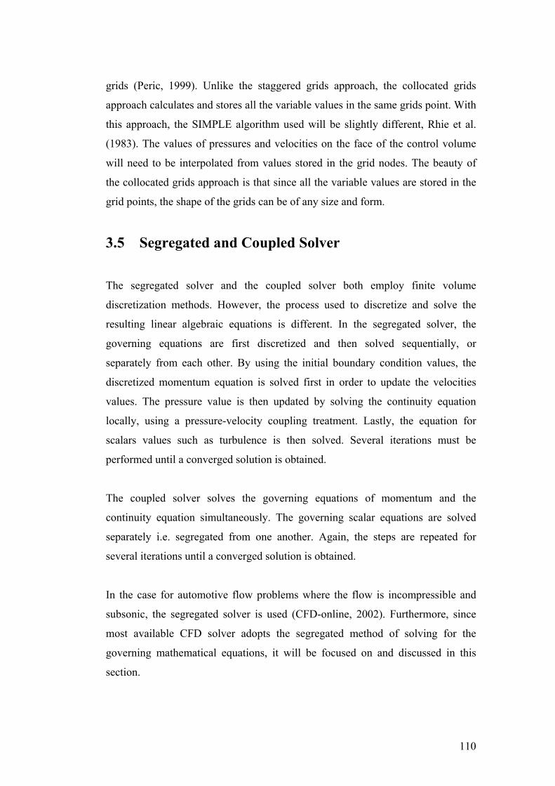
grids (Peric, 1999). Unlike the staggered grids approach, the collocated grids
approach calculates and stores all the variable values in the same grids point. With
this approach, the SIMPLE algorithm used will be slightly different, Rhie et al.
(1983). The values of pressures and velocities on the face of the control volume
will need to be interpolated from values stored in the grid nodes. The beauty of
the collocated grids approach is that since all the variable values are stored in the
grid points, the shape of the grids can be of any size and form.
3.5 Segregated and Coupled Solver
The segregated solver and the coupled solver both employ finite volume
discretization methods. However, the process used to discretize and solve the
resulting linear algebraic equations is different. In the segregated solver, the
governing equations are first discretized and then solved sequentially, or
separately from each other. By using the initial boundary condition values, the
discretized momentum equation is solved first in order to update the velocities
values. The pressure value is then updated by solving the continuity equation
locally, using a pressure-velocity coupling treatment. Lastly, the equation for
scalars values such as turbulence is then solved. Several iterations must be
performed until a converged solution is obtained.
The coupled solver solves the governing equations of momentum and the
continuity equation simultaneously. The governing scalar equations are solved
separately i.e. segregated from one another. Again, the steps are repeated for
several iterations until a converged solution is obtained.
In the case for automotive flow problems where the flow is incompressible and
subsonic, the segregated solver is used (CFD-online, 2002). Furthermore, since
most available CFD solver adopts the segregated method of solving for the
governing mathematical equations, it will be focused on and discussed in this
section.
110

This chapter describes the CFD pre-processing procedures for this project such as
the creation of CAD models, methods of grid generation and boundary conditions
used. In addition, this chapter also presents the most feasible grid generation
method used for simplified vehicle model with different windshield radii. This is
done through comparison of various grid generation methods.
3.6 Near Wall Models and Turbulence Models
The selections of near wall models available for this project are the Standard Wall
Function of Launder and Spalding (1974), Two Layer Wall Model of Chieng and
Launder (1980), Low Reynolds Wall Model of Lam and Bremhorst (1981), One
Equation Wall Model of Wolfstein (1969) and the Elliptic Blend model of
Manceau and Hanjalic (2002).
Launder and Spalding (1974) developed the standard wall function used in many
CFD applications used today. The development of the standard wall function was
based on combining Boussinesq assumptions with the Prandtl - Kolmogorov
relation for turbulent eddy viscosity in achieving the universal logarithmic law of
the wall in obtaining relationship for the mean velocity in the near wall region.
The calculation of mean velocity, together with the kinetic energy and dissipation
budget near to the wall will be based on the centre point of the cell adjacent to the
wall. The advantage of the standard wall function is to a certain extend provide a
robust and rudimentary solution to the near wall behaviour without requiring
extensive mesh refinements.
Chieng and Launder (1980) was the first to introduce the concept of two-layer
wall modelling in which the limit for the wall shear stress was set based on the
turbulent kinetic energy budget at the edge of the viscous sub-layer region. The
turbulent kinetic energy budget was determined through simultaneously modelling
the thickness and Reynolds number in the viscous sub-layer region. The main
benefit of using the wall treatment model was bypassing the need for mesh
integration right down throughout the viscous sub-layer region. Kim et al. (1995)
111

showed that under adverse pressure gradient conditions, the two-layer wall model
yielded an improved performance compared to the standard wall function of
Launder and Spalding (1974).
The model of Lam and Bremhorst (1981) is a low Reynolds number model
developed to complement the standard k-ε turbulence model in the near wall
region. The integration of this wall treatment model requires grid refinement all
the way to the viscous sub-layer region of the wall. This model includes
improvement to the damping function in the ε transport equation to account for
the change of turbulence length scale in the near wall region.
The enhanced wall treatment uses the Wolfstein (1969) one equation model is in
the low Reynolds number, viscous affected region. The modified version of the
Wolfstein (1969) model (FLUENT, 2003) uses a blending formulation in
modelling for the turbulent eddy viscosity in an effort to smooth the transition
between the fully turbulence and viscosity affected sub-layer region. The length
scale for the diffusion and dissipation term in the one equation model are also
assigned with damping factors to better model the viscosity affected region. The
one equation model has shown to offer good prediction in near wall flows due to
its empirical nature in providing a turbulence length scale to the flow, Wilcox
(2002).
The final wall treatment model that was chosen in this project was the Wall
Elliptic Blend model of Manceau and Hanjalic (2002) to complement the near
wall approach modelling strategy used together with the RSM of LRR and SSG.
The near wall treatment model was developed to satisfy the universal constraints
of turbulence properties close to the wall while at the same time maintaining the
simplistic approach to the numerical complexities of the model. This was done for
the main purpose of offering practicality for industrial applications. This was
achieved through modifying and simplifying the redistribution term in the
Reynolds Stress Near wall model of Durbin (1993) by using an elliptic blending
function.
112

The selections of turbulence models that were chosen for this project is the
standard k-ε, the k-ε RNG (Re-Normalization Group), Realizable k-ε and the k-ω,
Reynolds Stress Model (RSM) and the Hybrid Turbulence Model (HTM2).
The standard k – ε turbulence model of Launder and Spalding (1972), is the
standard turbulence model used in almost every CFD study as a baseline for
comparison with other turbulence model and will be chosen for this study. Due to
the use of Boussinesq postulations and eddy viscosity formulation for the
modelling of Reynolds stresses, the standard k – ε turbulence model is more suited
to modelling high Reynolds number flows type application, in which the
turbulence behaviour are more isotropic in nature. The stable and robust
characteristics of the standard k – ε turbulence model made it a popular choice
particularly for industrial application. Its deficiencies in modelling low Reynolds
number flow near to the wall and flow subjected to pressure gradient effects have
since been addressed by other researchers. Such effort to improve the standard k –
ε turbulence model includes the work of Yakhot and Orszag (1986) and Shih,
Liou, Shabbir, Yang and Zhu (1995).
Yakhot and Orszag (1986) conducted a study through the use of Re-
Normalization Group theory (RNG) in improving the standard k – ε turbulence
model. Improvements included the modification of the diffusion term in the k and
ε transport equation enabling it to perform better in near wall, separating and
swirling flows. In addition, an extra source term was introduced in the ε transport
equation that improves prediction of rapidly strained flows and the effect of
streamline curvature, FLUENT (2003). Validation of the RNG k – ε model by
Lien et al. (1994), Kim et al. (1995) and Wilcox (2002) showed an improve
performance over the standard k – ε model especially in adverse pressure
gradients flow.
Shih, Liou, Shabbir, Yang and Zhu (1995) introduced the “realizable” k – ε
turbulence model to address the non-physical turbulence characteristics displayed
by the standard and RNG k – ε turbulence model that occurred due to use of a
constant value of Cμ in modelling for the turbulent eddy viscosity. By using a
113

variable Cμ to better model the Reynolds stresses in flow situated close and far
away from the wall. The realizable k – ε also introduced a modified version of the
ε transport equation to better model the spreading rate of planar and round jet in
free shear flow, FLUENT (2003). The realizable k – ε turbulence model have
shown to perform better than the standard k – ε turbulence model in modelling
turbulent boundary layer flows, subjected to adverse pressure gradient effect that
includes separation and recirculation, Shih et al. (1995).
Wilcox (1998) developed the k-ω turbulence model in an attempt to provide a
superior choice in two-equation turbulence model over the k – ε turbulence model
family. By means of the perturbation method, Wilcox (2002) diagnosed the k-ω
model to reveal that the superior performance over the traditional k – ε turbulence
models was due to its ability to model the defect region within the boundary layer.
According to Wilcox (2002), successfully modelling the defect layer will
consequently result in better prediction of the transition and viscous sub-layer
region of the boundary layer. Validation by Wilcox (2002) for free shear flow
application showed better performance in comparison to the standard and RNG k
– ε turbulence model. The k-ω turbulence model was developed to perform down
to the viscous sub-layer region to account for low Reynolds number effects close
to the wall, requiring mesh refinement down to the viscous sub-layer region of the
wall.
The Hybrid Turbulence Model (HTM2) of Basara and Jakirlic (2002) was
developed behind the idea that the Cμ coefficient used to determine the turbulent
eddy viscosity varies across a wide range of turbulent flow and should remain
constant. Instead of using a standard constant for Cμ, the Cμ coefficient is taken as
a ratio between the production of turbulence kinetic energy of a Reynolds Stress
Model and a standard k – ε model. The variable values of Cμ suggested that the
HTM2 turbulence model should perform with the robustness of the standard k – ε
model while providing accuracy in results similar to the RSM turbulence model,
Basara et al. (2002).
114

The Reynolds stress turbulence model (RSM) used in AVL SWIFT CFD is of
Launder Reece and Rodi (LRR) (1975). The redistribution term used was that
developed by Speziale, Sarkar and Gatski (SSG) (1991). The RSM of LRR is the
most widely used second moment closure turbulence model. Its advantages
include improvement over the eddy viscosity models in predicting complex three
dimensional flow that are subjected to curved surfaces, swirl, rotation, rapid
variation of strain rate and boundary layer separation, FLUENT (2003), Wilcox
(2002). These are implemented by modelling Reynolds stresses via transport
equations, by passing the traditional method of the Eddy Viscosity method. The
combination of LRR and SSG as an RSM provides a superior performance in a
variety of complex flow over the standard LRR model, Speziale et al. (1991) and
Basara et al. (2003).
3.7 CAD Model Geometry and Boundary Conditions
Input
The CFD models used for this project were based on five different simplified
vehicle model (40% scale) of Alam (2000). The models are different form each
other in terms of their A-pillar windshield radius configuration. Alam (2000)
defined the five simplified vehicle models as:
• Rectangular Edge (RE)
• Slanted Edge (SL)
• Semi Circular (Semi)
• Small Ellipsoidal (SE)
• Large Ellipsoidal (LE)
115
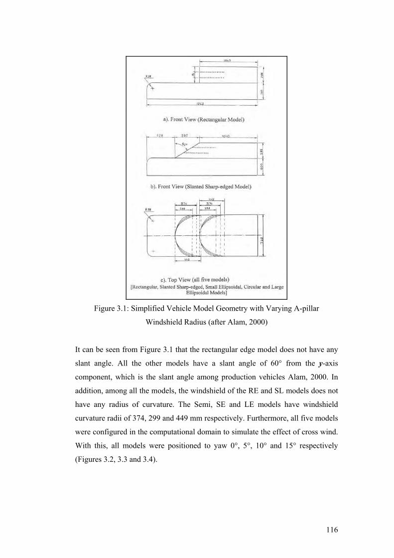
Figure 3.1: Simplified Vehicle Model Geometry with Varying A-pillar
Windshield Radius (after Alam, 2000)
It can be seen from Figure 3.1 that the rectangular edge model does not have any
slant angle. All the other models have a slant angle of 60° from the y-axis
component, which is the slant angle among production vehicles Alam, 2000. In
addition, among all the models, the windshield of the RE and SL models does not
have any radius of curvature. The Semi, SE and LE models have windshield
curvature radii of 374, 299 and 449 mm respectively. Furthermore, all five models
were configured in the computational domain to simulate the effect of cross wind.
With this, all models were positioned to yaw 0°, 5°, 10° and 15° respectively
(Figures 3.2, 3.3 and 3.4).
116

0 Yaw 5 Yaw
15 Yaw 10 Yaw
Figure 3.2: Models in 0°, 5°, 10° and 15° yaw position
Figure 3.3: Small Ellipsoidal Model in a yaw position within Computational
Domain in AVL
117
Figure 3.4: Slanted Edge Model within Computational Domain in FLUENT
All five models were given a length of the bottom 1963 mm, a width of 748 mm
and height of 300 mm. The canopy or top section of the models are 288 mm in
dimension and contains two rows of pressure tapping points, which are 96 mm
from each other. For the RE and SL model, the first pressure tapping point is
situated 384 mm from the centre of the windshield or 10 mm from the edge of the
A-pillar. For the Semi, SE and LE models, the first pressure tapping point is
situated at 490, 470 and 530 mm from the centre of the windshield respectively.
Each row consists of 16 pressure-tapping points and each point is 32 mm apart
from each other (Figure 3.1).
The computational domain that surrounds the CFD model is generated base on the
dimension of the RMIT University wind tunnel in Melbourne, Australia. The
RMIT wind tunnel dimensions were measured at 9.0 metres in length, 3.0 metres
in width and 2.0 metres in height.
The computational domain and the simplified vehicle CFD models were generated
to be simulated using FLUENT and AVL. For FLUENT, a geometry and mesh
builder called GAMBIT (version 1.3) was used, which is also a product developed
by FLUENT Incorporated. CAD models generated in GAMBIT were saved in a
DBS file before being used for grid generation. For AVL, AUTOCAD was used
to generate all the CAD models. The CAD models are then saved in an STL file
before being exported to AVL for grid generation. The CAD models generated for
FLUENT and AVL can be seen in Figure 3.5 and 3.6 respectively.
118

Figure 3.5: Semi Circular Model within Computational Domain in AVL
Figure 3.6: Slanted Edge Model with Multi-block volumes in GAMBIT
Before a CFD simulation can be conducted, appropriate boundary condition
values must first be specified to the CFD solver. Three separate set of simulation
was carried out at vehicle speeds of 60, 100 and 140 km/h respectively. The
boundary condition values were specified at the inlet face of the computational
domain velocity inlet. This correspond to Reynolds number of 2.169 x 10⁶, 3.615
x 106 and 5.061 x 10⁶ respectively. The boundary condition at the outlet face of
the computational domain was set as pressure outlet.
119
In FLUENT, the convection scheme and the pressure-velocity coupling used for
the simulation was set as first and second order upwind differencing scheme and
SIMPLE scheme respectively. Default under-relaxation values were used. The
convergence level for the residuals for the simulation was set at 0.1%. Throughout
the calculation, under-relaxation values were reduced whenever solution showed
instability and divergence. The reduction of under-relaxation values varies from
one simulation to the other and depends on such factors as inlet velocity,
convection scheme used and turbulence model used.
In AVL, the simulation was first carried out using first order upwind scheme and
central differencing scheme. Once convergence was reached, the AVL Smart
Bound higher order scheme was then used. This was done by progressively
altering the blend factor constant in the differencing scheme option. For the higher
order scheme was used with a 0.5 blend factor. The convergence level was set to
0.1% with SIMPLE used as the pressure-velocity coupling scheme. The reduction
of under-relaxation values also varies from one simulation to the other.
For the turbulence models used, initial guess values were specified for the
turbulence kinetic energy (k) and dissipation rate (ε), which was determined from
the formula of turbulence intensity and dissipation length scale. The turbulent
intensity was taken as 1.8% (based on Alam, 2000) and the dissipation length
scale was based from 1.0% of the simplified vehicle model height, which resulted
in 5.88 mm. These equations are defined as:
32
23 ,inlet
k C kI l
vμ
ε ε= = (3.3)
For the three inlet velocities, 60, 100 an140 km/h, this resulted in the guessed
values of 0.135, 0.375 and 0.735 for k and the values of 0.759, 3.515 and 9.645
for ε.
120

The summary of the boundary conditions, numerical scheme along with the
turbulence and near wall model used for FLUENT and AVL are listed in Table
3.1 and 3.2.
Table 3.1: Boundary conditions, numerical schemes, turbulence and near wall
model for FLUENT
Inlet Boundary Conditions Velocity Inlet at 60, 100 and 140 km/h
Outlet Boundary Conditions Pressure Outlet
Yaw Angles 0°, 5°, 10° and 15°
Convection Scheme First order and Second order upwind convection
scheme
Pressure-Velocity Coupling
Scheme
SIMPLE
Turbulence Model Standard k-ε (initial), k-ε RNG (Re-Normalization
Group), Realizable k-ε and k-ω
Near Wall Model Hybrid Grids with One Equation Model of
Wolfstein (1969)
Convergence Level 0.1%
Turbulence Intensity Used 1.8%
Length Scale Used 5.8mm (1.0% of vehicle height)
121
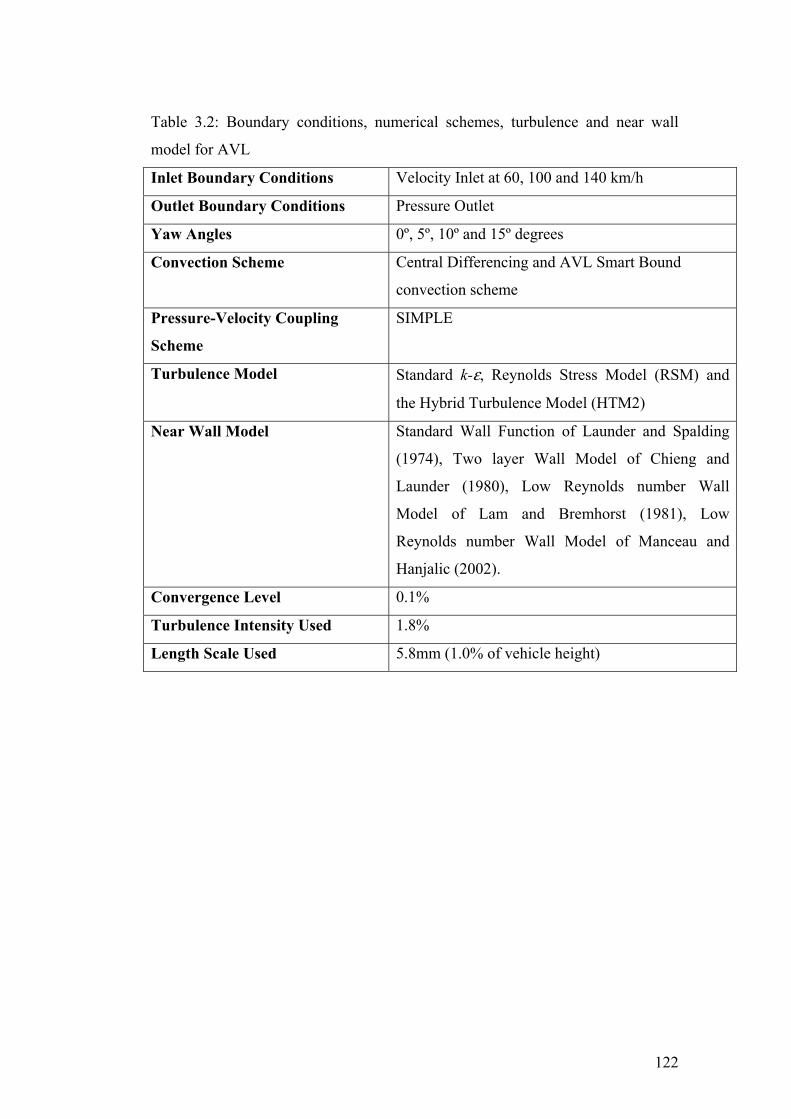
Table 3.2: Boundary conditions, numerical schemes, turbulence and near wall
model for AVL
Inlet Boundary Conditions Velocity Inlet at 60, 100 and 140 km/h
Outlet Boundary Conditions Pressure Outlet
Yaw Angles 0º, 5º, 10º and 15º degrees
Convection Scheme Central Differencing and AVL Smart Bound
convection scheme
Pressure-Velocity Coupling
Scheme
SIMPLE
Turbulence Model Standard k-ε, Reynolds Stress Model (RSM) and
the Hybrid Turbulence Model (HTM2)
Near Wall Model Standard Wall Function of Launder and Spalding
(1974), Two layer Wall Model of Chieng and
Launder (1980), Low Reynolds number Wall
Model of Lam and Bremhorst (1981), Low
Reynolds number Wall Model of Manceau and
Hanjalic (2002).
Convergence Level 0.1%
Turbulence Intensity Used 1.8%
Length Scale Used 5.8mm (1.0% of vehicle height)
122

Chapter Four
RANS CFD SIMULATION OF A-PILLAR
AERODYNAMICS
This chapter is divided into two main sections. The first section presents the CFD
model development for this project. The second section presents the results and
discussion of the A-pillar aerodynamics obtained from the CFD model developed.
Validation of the CFD results against the experimental dara are also presented in
the second section.
4.1 Objective and Scope of this Chapter
From the knowledge obtained while researching for this project through reviews
of literatures, the following questions were raised and will be addressed in this
chapter.
What are the most suitable combination of grid, near wall model and
turbulence model to use for the CFD model in the project?
How accurate are the proposed turbulence and near wall model in terms of
percentage error values? Are the errors within acceptable values?
Using flow visualisation, what are the physical characteristics and
mechanism of vortices generated from the A-pillar aerodynamics?
Using flow visualisation, how do different vehicle windshield radii
configurations affect A-pillar aerodynamics together with the vortices and
turbulence generation associated with it?
123
Therefore, the main objectives of this chapter are twofold:
1. To develop a CFD model for the project by obtaining the best combination
of grid, near wall model and turbulence model for the various windshield
radii and yaw angle. CFD model results were validated against the existing
experimental data of Alam (2000).
2. To examine the aerodynamics behaviour behind the A-pillar region using
the developed CFD model by means of elucidating the mechanism of
turbulence generation and airflow physical characteristics from the various
flow conditions through further justifications with relevant works of
literatures.
4.2 CFD Model Development
Development of the CFD model will be discussed in this section. This includes
the combination for the most feasible grid, near wall model and turbulence model.
4.2.1 Grid Feasibility Study – Generation Technique
Different grid generation methods were used to mesh the CFD models in both
GAMBIT and AVL. The grid generation methods differ from each other based on
two factors, the difficulty of the method and also on the accuracy that each
method provides. The grid generation methods used were categorised into either a
conformal or non-conformal generation. The conformal grid generation technique
used comprised of either using structured or unstructured grids. The non-
conformal grid generation technique used comprised of using the multiblock grid
technique.
In GAMBIT, both the non-conformal and conformal grid generation techniques
were implemented. For this project, the non-conformal multiblock grid generation
124

technique was constructed using fully hexahedral grids and hybrid grids. The
conformal grid generation technique was constructed using fully unstructred
tetrahedral grids.
The non-conformal multiblock grid generation technique usedin GAMBIT was
the most difficult to implement. They can be constructed using fully hexahedral
grids or a combination of hexahedral, prismatic and tetrahedral grids, which
combination are often known as hybrid grids. In the multiblock technique, the
entire computational domain can be divide into several volume blocks. Each
adajacent blocks are connected via an interface boundary condition with each
block meshed independently. Generating grids using the multiblock techniques
can be a problem in GAMBIT because the interface boundary conditions might
fails to connect if the adjacent blocks are too big. In the case for the multiblock
technique, smoothing technique must also be applied between adjacent blocks in
order to prevent numerical instability. The slanted edge model implemented with
the multi block grid generation technique can be seen in Figure 4.1.
Figure 4.1: Slanted Edge Model with Multi-block volumes in GAMBIT
The fully structured hexahedral grids generated by using the multi block
technique possess the highest grid quality due to its conformity with the aspect
125

ratio and skewness angle requirement. Mesh analysis from GAMBIT showed that
only 0.05% grids are outside the aspect ratio requirement and 0.8% grids are
outside the skewness angle requirement respectively. This should minimise
discretization error and most often than not, translate to accurate CFD results.
However, the generation of hexahedral grids throughout the computational
domain was an expensive exercise. The structured arrangement of the hexahedral
grids required fine grids to be generated in areas within the computational
domain, often located in the non-critical flow region. This is inappropriate since
maximum accuracy is only needed for this project on the area surrounding the A-
pillar region. Therefore, an alternative to using the fully structured hexahedral
grids is to use hybrid grids in order to obtain a more efficient grid distribution
throughout the computational domain. The fully structured hexahedral grids
layout can be seen in Figure 4.2 with the mesh quality can be seen in Figure 4.3.
Figure 4.2: Fully Structured Hexahedral Grids Layout in GAMBIT
Figure 4.3: Grid Skewness Quality of the Fully Structured Hexahedral Grids in
GAMBIT
126

The hybrid grids generated using the multiblock technique are a combination of
hexahedral, prismatic and tetrahedral grids. The area surrounding the surface of
the vehicle model was meshed using hexahedral grids while the surrounding area
was meshed using tetrahedral grids. Prismatic grids were used to connect the
hexahedral and tetrahedral grids respectively. The reason to generate hexahedral
grids surrounding the surface of the model was to obtain maximum accuracy,
particularly around the A-pillar region. Furthermore, hexahedral grids are also
needed near the surrounding model surface in order to successfully generate fine
boundary layer mesh for simulating laminar flow in the sub-layer region.
Everywhere else within the computational domain, tetrahedral grids were
generated. Due to its unstructured arrangement, less grids were used to generate
tetrahedral grids in which, reasonable accuracy can be obtained. Mesh analysis
from GAMBIT showed that 24.6% grids are outside the aspect ratio requirement
and 20.7% grids are outside the skewness angle requirement respectively. The
reason for the high number of increase in aspect ratio percentage is due to the
generation of boundary layer close to the model surface. The high increase of
skewness angle however, is due to the generation of tetrahedral grids outside the
critical of the flow. The hybrid grids layout can be seen in Figure 4.4 with the
mesh quality can be seen in Figure 4.5.
Figure 4.4: Hybrid Grids Layout in GAMBIT
127

Figure 4.5: Grid Skewness Quality of the Hybrid Grids in GAMBIT
In the conformal grid generation technique used in GAMBIT, fully unstructured
tetrahedral grids were used. They are the easiest to generate in comparison to the
fully structured hexahedral and hybrid grids. However, the unstructured
tetrahedral grids are low in quality since it has high skewness and aspect ratio.
This might result in high discretization error, especially when exposed to A-pillar
vortex flow. Mesh analysis from GAMBIT showed that none of the grids are
outside the aspect ratio requirement and 27.0% grids are outside the skewness
angle requirement respectively. The reason for the low percentage of aspect ratio
is due to the generation of purely tetrahedral grids. The percentage of skewness
angle is similar as per the hybrid method in which is caused by the generation of
tetrahedral grids in the computational domain. The unstructured tetrahedral grids
layout can be seen in Figure 4.6 with the mesh quality can be seen in Figure 4.7.
Figure 4.6: Unstructured Tetrahedral Grids Layout in GAMBIT
128

Figure 4.7: Grid Skewness Quality of the Unstructured Tetrahedral Grids in
GAMBIT
In AVL, a built in grid generator tool call Fame Hybrid was used. Fame Hybrid
uses a more advance meshing system called the Arbitrary Cell Technology
(ACT). In the ACT meshing system, a blend of conformal polyhedral grids can be
used to mesh and refine complex 3-D CFD models. The grid generation procedure
can be done either manually or by using an automatic grid generator. In
comparison to GAMBIT, highly complex grids can be generated easier by using
Fame Hybrid and without having to use the multiblock technique. The resulting
mesh quality is probably similar to those of Hybrid grids from Gambit. The
polyhedral grids layout from Fame Hybrid can be seen in Figure 4.8.
129

Figure 4.8: ACT Polyhedral Grids Layout in AVL generated using Fame Hybrid
For this project, the non-conformal fully structured hexahedral in GAMBIT were
implemented only on the sharp edge models (RE and SL) at 0° yaw due to its
tedious and difficult nature of generation. The non-conformal hybrid grids and
conformal unstructured tetrahedral grids in GAMBIT were implemented to the
sharp edge models (RE and SL), along with the circular models (Semi, SE and
LE) at 0°, 5°, 10° and 15° yaw. In AVL, polyhedral grids generated by using
Fame Hybrid was applied to the sharp edge (RE and SL) and circular models
(Semi, SE and LE) at 0°, 5°, 10° and 15° yaw.
Implementation of the various grid generation techniques shows that the
tetrahedral and the AVL polyhedral grids are the easiest to generate among all the
grid generation methods used. In the next section, we shall look on the accuracy
and the applicability of these grid generation methods.
130

A summary listing the grid generation techniques used for both the models in
GAMBIT and AVL Fame Hybrid are as follows:
GAMBIT
o Non-Conformal Hexahedral – Sharp Edge models at 0° yaw.
o Conformal Tetrahedral – Sharp Edge and Circular models at 0°, 5°,
10° and 15° yaw.
o Non-Conformal Hybrid – Sharp Edge and Circular Models at 0°,
5°, 10° and 15° yaw.
AVL Fame Hybrid
o Polyhedral ACT – Sharp Edge and Circular models at 0°, 5°, 10°
and 15° yaw.
4.2.2 Grid Feasibility Study – Grid Refinement &
Independency Procedure
Initial grids generated in GAMBIT and AVL Fame Hybrid are coarse. The coarse
grids were then subjected to a grid independency test. In the grid independency
test, grids were repeatedly refined especially in areas with high variable flow
gradients until less than 5.0% in error was achieved relative to the results from
previous refinement. For this project, only models subjected to yaw of 0° and 15°
were used for the grid independency testing, to investigate least and worse case
airflow scenario.
For the grid independency test, the CFD models generated using the non-
conformal and conformal grid method in GAMBIT were subjected to a wind
tunnel inlet velocity of 60 km/h. Standard k-ε turbulence model was used for the
simulation. For models meshed using the non-conformal grid method (hexahedral
and hybrid), the modeling was done in two scenarios, with and without boundary
layer grids added to the wall. In the scenario with boundary layer grids, near wall
conditions for the grid independency test for FLUENT was conducted using
131

Wolfstein (1967, 1969) one equation model. In the scenario without the boundary
layer grids, and this also applies to the models meshed with conformal
unstructured grid method, wall conditions were of the non-equilibrium wall
function model.
For AVL Fame Hybrid, all CFD models were subjected to an inlet velocity of 60
km/h. Standard k-ε turbulence model with standard near wall function model was
used. Boundary layer grids were later added to the sharp edge models at 0° yaw
and for all models at 15° yaw. Near wall conditions for the grid independency test
was then conducted using Lam et al. (1981) low Reynolds number model.
In GAMBIT, the grid refinement for the conformal unstructured grids was made
through automatic solution adaptation technique. For the non-conformal
hexahedral and hybrid grids, the final amount and combination of grids generated
was based on the grid refinement obtained from the grid independency test done
on the polyhedral grids (which is similar to hybrid grids) in AVL.
The initial surface grid size created on the vehicle models wall surface (before
refinements) for the unstructured tetrahedral in GAMBIT was 20 mm in size
while the surface grid on the tunnel wall was 200 mm in size. For the hexahedral
and hybrid grids, the final grids generated on the vehicle wall surface was 20 mm
with surface grids surrounding the A-pillar region generated at 5 mm in size. For
models constructed using the fully unstructured tetrahedral grid method, the total
initial grids generated was around 250,000. The final grid total after achieving
grid independcy was around 500,000 (Refer to Figure 4.9). For models generated
using the hexahedral and hybrid grid method, the final grids generated was around
1.0 million with 477,000 grids generated on each side of the A-pillar region.
132

Figure 4.9: Before and After Solution Adaptive Refinement for Semi Circular
For the hybrid grid strategy, boundary layer mesh was added to better capture the
airflow in the boundary layer region in order to obtain a more accurate static
pressure distribution on the vehicle surface. The first boundary layer mesh point
was at 0.03 mm perpendicular to the vehicle surface resulting in the y+ value close
to the wall to be close to 1. A total of 14 boundary layer mesh was generated in
1.4 ratio increments resulting to a total depth of 8.3mm. The final grids generated
along with added boundary layer grids for the sharp edge model totalled to
approximately 1.4 million (Refer to Figure 4.10)
133

Boundary Layer Mesh
Figure 4.10: Boundary Layer Grids for the Slanted Edge Model generated using the Hybrid Grids Method in GAMBIT
In AVL, an initial coarse wall surface grids of 200 mm in size was generated on
the wind tunnel wall. For all models, an initial surface mesh of 100 mm in size
was generated on the vehicle model surface. The wall surface mesh was later
refined to 50 mm, 25 mm and 12.5 mm in size respectively. However, on the
slanted edge model at 0° yaw and for all models at 15° yaw, a further refinement
was conducted on the wall surface surrounding the A-pillar region with generated
grid size of 5.0 mm in size. In addition, a choice of 5 and 10 boundary layer grids
were constructed on the models surfaces with the first grid next to the wall
measuring 0.1 and 0.01 mm in size respectively. The y+ value close to the wall
obtained after the addition of boundary layer grids was less than 1. Grid
independency test for AVL was conducted using the re-meshing technique. Using
this technique, new sets of refined grids were generated after a converged solution
were obtained from previous set of grids and repeated until error of results were
restricted to a maximum of 5.0% relative to previous refinement results. The
initial coarse grids generated using Fame Hybrid for the models at 0° yaw was
around 20,000, which was far less than the total grid count from GAMBIT. The
final grid count after grid independency test for the circular models was around
200,000 grids (Refer Figure 4.11). For the sharp edge model at 0° yaw and all
models at 15° yaw, the final grid refinement was done at around 1.7 million grids
with minimum improvement. At this point, a combination of either 5 or 10
134

boundary layer grids were added to the fourth and fifth grid refinement in a
different approach to obtain grid independency (Refer Figure 4.12).
Figure 4.11: Grid Independency Test for the Semi Circular Model in AVL at 0° Yaw
135

Figure 4.12: Grid Independency Test for the Semi Circular Model in AVL at 15°
Yaw
A summary listing the initial and final grid refinement used for both the models in
GAMBIT and AVL Fame Hybrid through the grid independency testing
procedure are as follows:
GAMBIT
o Fully Unstructured Tetrahedral Grids generated on the Circular and
Sharp Edge models – Initial 250,000; Final 500,000.
o Fully Hexahedral and Hybrid Grids generated on the Circular and
Sharp Edge models – Initial 250,000; Final 1 million (without
boundary layer), 1.4 million (with boundary layer).
136

AVL Fame Hybrid
o Circular models at 0° yaw – Initial 20,000; Final 200,000.
o Sharp Edge models at 0° and 15° yaw, Circular models at 15° yaw
– Initial 20,000; Final 1.7 million.
4.2.3 Grid Feasibility Study – Validation with
Experimental Results at 0° Yaw
The grid independency test results obtained for the circular models at 0° yaw
compared against the experimental results of Alam (2000). From Figures 4.13 to
4.14, it can be seen that close agreements were obtained with experimental results
for models simulated using FLUENT and AVL SWIFT. However, a more
consistent prediction was obtained using AVL SWIFT. From the results obtained
from FLUENT and AVL SWIFT, the most feasible grid generation method to be
implemented for future CFD modelling of the circular models at 0° yaw are by
using the Fame Hybrid polyhedral grids with standard wall function. Apart from
the overall consistency that was obtained by using this method, this strategy was
also chosen because it is easy to generate and uses only around 200,000 grids,
which was almost half the total final grid count to FLUENT (around 500,000).
137
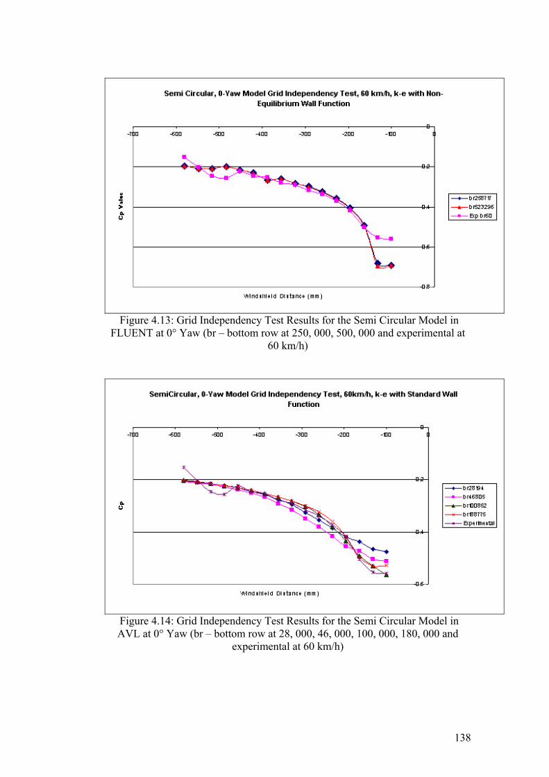
Figure 4.13: Grid Independency Test Results for the Semi Circular Model in FLUENT at 0° Yaw (br – bottom row at 250, 000, 500, 000 and experimental at
60 km/h)
Figure 4.14: Grid Independency Test Results for the Semi Circular Model in AVL at 0° Yaw (br – bottom row at 28, 000, 46, 000, 100, 000, 180, 000 and
experimental at 60 km/h)
138

The results from the grid refinements of the sharp edge models at 0° yaw were
compared to the experimental results of Alam (2000). From Table 4.1 and Figures
4.15, 4.16 and 4.17, it can be seen that among the grid generation methods used in
FLUENT, the Hybrid grids with boundary layer yields the least discrepancy
against results obtained experimentally. The overall discrepancy obtained was
26.1%. This followed by the Hexahedral, Hybrid with no boundary layers and
tetrahedral grids generation methods, with overall discrepancy of 35.6%, 40.0%
and 41.2% respectively. For the grid generation method implemented in AVL
SWIFT, it can be seen from Table 4.1 and Figure 4.14 that the Polyhedral Grids
with boundary layers yields the least discrepancy against experimental results
with 21.9% overall discrepancy. The Polyhedral Grids without boundary layers
yields an overall discrepancy of 38.7%.
Figure 4.15: Comparison between Hexahedral, Hybrid and Tetrahedral Grid Generation Method in FLUENT at 0° Yaw
139

Figure 4.16: Grid Independency Test Results for the Slanted Edge Model in AVL at 0° Yaw with Standard Wall Function (br – bottom row at 13, 000, 34, 000, 107,
000, 199, 000, 820, 000, 1.5 million and experimental at 60 km/h)
From the analysis of all the grid generation methods employed for the sharp edge
model at 0º yaw, it can be concluded that the most feasible method chosen is the
Polyhedral Grids with boundary layers, which was generated using AVL SWIFT.
The polyhedral grids were chosen because it was easy to generate having the least
overall discrepancy. The amount of grids generated was similar to methods used
in FLUENT. This grid generation method will be used in AVL SWIFT to assess
the performance of various near wall and turbulence models. The hybrid grids
with boundary layers will be used to assess the performance of various near wall
and turbulence models in FLUENT.
140

Figure 4.17: Comparison between Hybrid and Polyhedral Grids at High and Low Reynolds Number Conditions
141
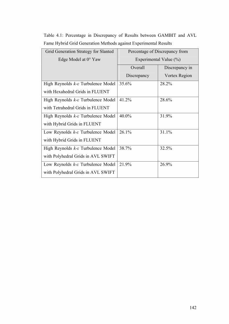
Table 4.1: Percentage in Discrepancy of Results between GAMBIT and AVL
Fame Hybrid Grid Generation Methods against Experimental Results
Percentage of Discrepancy from
Experimental Value (%)
Grid Generation Strategy for Slanted
Edge Model at 0° Yaw
Overall
Discrepancy
Discrepancy in
Vortex Region
High Reynolds k-ε Turbulence Model
with Hexahedral Grids in FLUENT
35.6% 28.2%
High Reynolds k-ε Turbulence Model
with Tetrahedral Grids in FLUENT
41.2% 28.6%
High Reynolds k-ε Turbulence Model
with Hybrid Grids in FLUENT
40.0% 31.9%
Low Reynolds k-ε Turbulence Model
with Hybrid Grids in FLUENT
26.1% 31.1%
High Reynolds k-ε Turbulence Model
with Polyhedral Grids in AVL SWIFT
38.7% 32.5%
Low Reynolds k-ε Turbulence Model
with Polyhedral Grids in AVL SWIFT
21.9% 26.9%
142
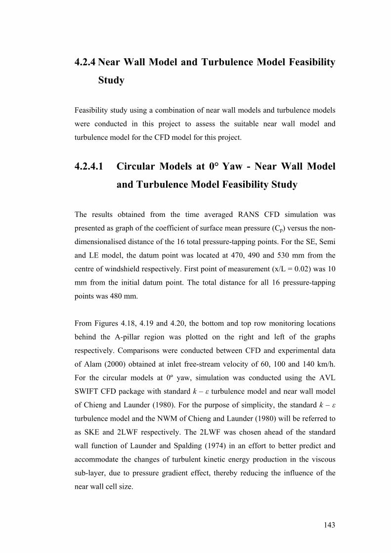
4.2.4 Near Wall Model and Turbulence Model Feasibility
Study
Feasibility study using a combination of near wall models and turbulence models
were conducted in this project to assess the suitable near wall model and
turbulence model for the CFD model for this project.
4.2.4.1 Circular Models at 0° Yaw - Near Wall Model
and Turbulence Model Feasibility Study
The results obtained from the time averaged RANS CFD simulation was
presented as graph of the coefficient of surface mean pressure (Cp) versus the non-
dimensionalised distance of the 16 total pressure-tapping points. For the SE, Semi
and LE model, the datum point was located at 470, 490 and 530 mm from the
centre of windshield respectively. First point of measurement (x/L = 0.02) was 10
mm from the initial datum point. The total distance for all 16 pressure-tapping
points was 480 mm.
From Figures 4.18, 4.19 and 4.20, the bottom and top row monitoring locations
behind the A-pillar region was plotted on the right and left of the graphs
respectively. Comparisons were conducted between CFD and experimental data
of Alam (2000) obtained at inlet free-stream velocity of 60, 100 and 140 km/h.
For the circular models at 0º yaw, simulation was conducted using the AVL
SWIFT CFD package with standard k – ε turbulence model and near wall model
of Chieng and Launder (1980). For the purpose of simplicity, the standard k – ε
turbulence model and the NWM of Chieng and Launder (1980) will be referred to
as SKE and 2LWF respectively. The 2LWF was chosen ahead of the standard
wall function of Launder and Spalding (1974) in an effort to better predict and
accommodate the changes of turbulent kinetic energy production in the viscous
sub-layer, due to pressure gradient effect, thereby reducing the influence of the
near wall cell size.
143
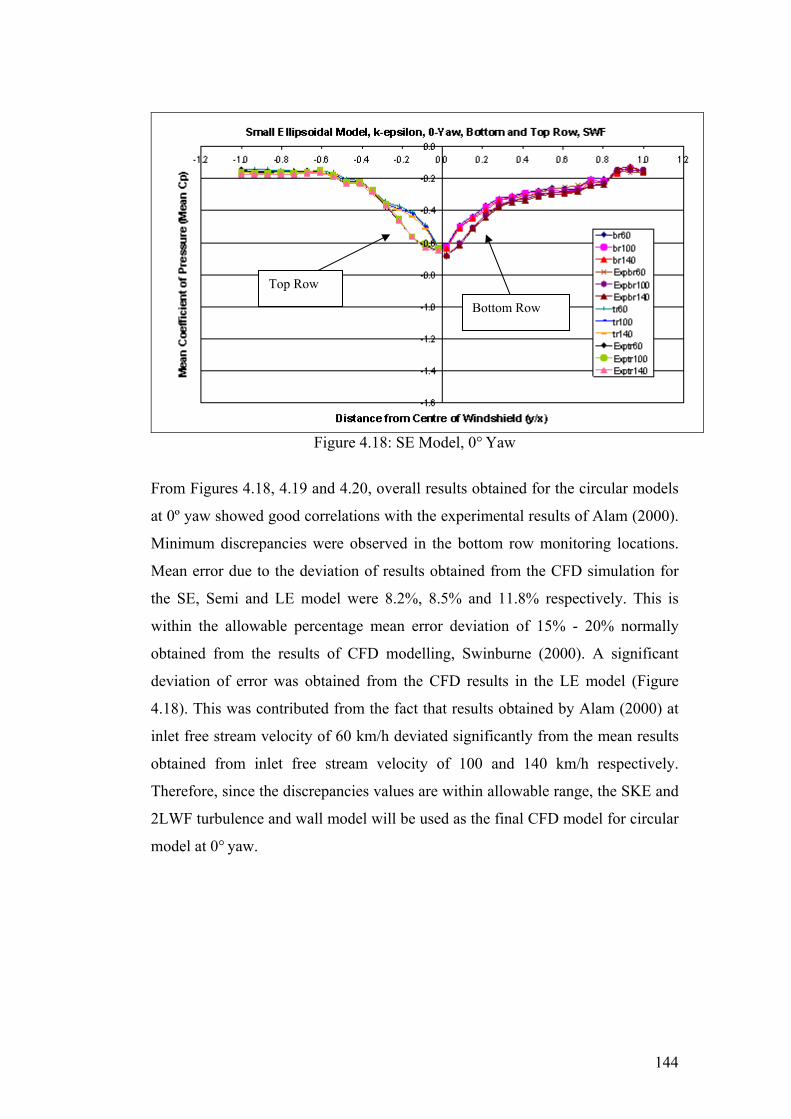
Top Row
Bottom Row
Figure 4.18: SE Model, 0° Yaw
From Figures 4.18, 4.19 and 4.20, overall results obtained for the circular models
at 0º yaw showed good correlations with the experimental results of Alam (2000).
Minimum discrepancies were observed in the bottom row monitoring locations.
Mean error due to the deviation of results obtained from the CFD simulation for
the SE, Semi and LE model were 8.2%, 8.5% and 11.8% respectively. This is
within the allowable percentage mean error deviation of 15% - 20% normally
obtained from the results of CFD modelling, Swinburne (2000). A significant
deviation of error was obtained from the CFD results in the LE model (Figure
4.18). This was contributed from the fact that results obtained by Alam (2000) at
inlet free stream velocity of 60 km/h deviated significantly from the mean results
obtained from inlet free stream velocity of 100 and 140 km/h respectively.
Therefore, since the discrepancies values are within allowable range, the SKE and
2LWF turbulence and wall model will be used as the final CFD model for circular
model at 0° yaw.
144

Figure 4.19: Semi Model, 0° Yaw
Figure 4.20: LE Model, 0° Yaw
145

4.2.4.2 Circular Models at 5°, 10° and 15º Yaw – Near
Wall Model and Turbulence Model Feasibility
Study
In this section, comparison between turbulence model of SKE, HTM2, k – ω and
RSM was conducted using their respective accompanying near wall model. For
the SKE turbulence model, the low Reynolds number model of Lam and
Bremhorst (1981) will be used. For the purpose of simplicity, the low Reynolds
number model of Lam and Bremhorst (1981) will be referred to as the LB model.
The Wilcox (1998) k – ω turbulence model didn’t require any near wall model to
model near wall effect since the turbulence model was developed to handle
modelling of near wall effect. The RSM will be modelled using the Wall Elliptic
Blend model of Manceau and Hanjalic (2002). For the purpose of simplicity, Wall
Elliptic Blend model of Manceau and Hanjalic (2002) will be referred to as the
WEB model. Finally, the HTM2 turbulence model will be modelled using the
2LWF near wall model. Although the 2LWF near wall model does not require
mesh refinement all throughout until the viscous sub-layer, the attractiveness of
this turbulence model in offering the combination of the SKE and RSM model
obtained the inclusion in this investigation. For simplicity, the turbulence models
and their respective near wall model will be referred to as the SKE-LB model, the
k – ω model, the HTM2-2LWF model and the RSM-WEB model. The turbulence
models and their respective near wall model assessment were conducted at yaw
angles of 5°, 10° and 15° and at 140 km/h. Comparisons were made against the
experimental data of Alam (2000).
146

Leeward Region Windward
Region
Figure 4.21: SE Model, 5° Yaw, Bottom Row, Turbulence Model Comparison
Figure 4.22: SE Model, 10° Yaw, Bottom Row, Turbulence Model Comparison
147

Figure 4.23: SE Model, 15° Yaw, Bottom Row, Turbulence Model Comparison
Figures 4.21 showed results obtained for the SE model at 5° yaw. Figures 4.22
correspond to SE model at 10° yaw while figures 4.23 correspond to SE model at
15° yaw respectively. From the Figures at 5° yaw, the SKE-LB model, HTM2-
2LWF model, k – ω model and RSM-WEB model produced an overall mean
percentage error deviation of 20.5%, 20.0%, 18.9% and 16.8% from the
experimental results respectively. From the comparisons, it can be seen that the
RSM-WEB model produced the best result in predicting the flow phenomena
behind the A-pillar region for the SE model at 5° yaw. At 10° yaw, the SKE-LB
model, HTM2-2LWF model, k – ω model and the RSM-WEB model produced an
overall mean percentage error deviation of 26.2%, 19.2%, 20.7% and 18.8% from
the experimental results respectively. From the turbulence model comparisons, it
can be seen that the RSM-WEB model produced the best result in predicting the
flow phenomena behind the A-pillar region for the SE model at 10° yaw. CFD
modelling results obtained at 15° yaw was similar as the ones obtained at 10º yaw.
The SKE-LB model, HTM2-2LWF model, k – ω model and the RSM-WEB
model produced an overall mean percentage error deviation of 32.1%, 26.3%,
28.9% and 20.3% from the experimental results respectively. From the turbulence
model comparisons, it can be seen that the RSM-WEB model produced the best
148

result in predicting the flow phenomena behind the A-pillar region for the SE
model at 15° yaw.
Figure 4.24: Semi Model, 5° Yaw, Bottom Row, Turbulence Model Comparison
Figure 4.25: Semi Model, 10° Yaw, Bottom Row, Turbulence Model Comparison
149
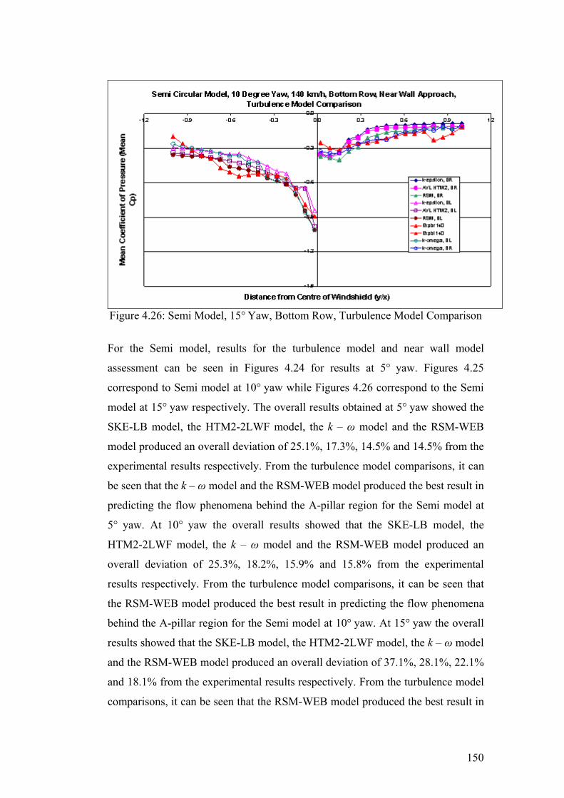
Figure 4.26: Semi Model, 15° Yaw, Bottom Row, Turbulence Model Comparison
For the Semi model, results for the turbulence model and near wall model
assessment can be seen in Figures 4.24 for results at 5° yaw. Figures 4.25
correspond to Semi model at 10° yaw while Figures 4.26 correspond to the Semi
model at 15° yaw respectively. The overall results obtained at 5° yaw showed the
SKE-LB model, the HTM2-2LWF model, the k – ω model and the RSM-WEB
model produced an overall deviation of 25.1%, 17.3%, 14.5% and 14.5% from the
experimental results respectively. From the turbulence model comparisons, it can
be seen that the k – ω model and the RSM-WEB model produced the best result in
predicting the flow phenomena behind the A-pillar region for the Semi model at
5° yaw. At 10° yaw the overall results showed that the SKE-LB model, the
HTM2-2LWF model, the k – ω model and the RSM-WEB model produced an
overall deviation of 25.3%, 18.2%, 15.9% and 15.8% from the experimental
results respectively. From the turbulence model comparisons, it can be seen that
the RSM-WEB model produced the best result in predicting the flow phenomena
behind the A-pillar region for the Semi model at 10° yaw. At 15° yaw the overall
results showed that the SKE-LB model, the HTM2-2LWF model, the k – ω model
and the RSM-WEB model produced an overall deviation of 37.1%, 28.1%, 22.1%
and 18.1% from the experimental results respectively. From the turbulence model
comparisons, it can be seen that the RSM-WEB model produced the best result in
150
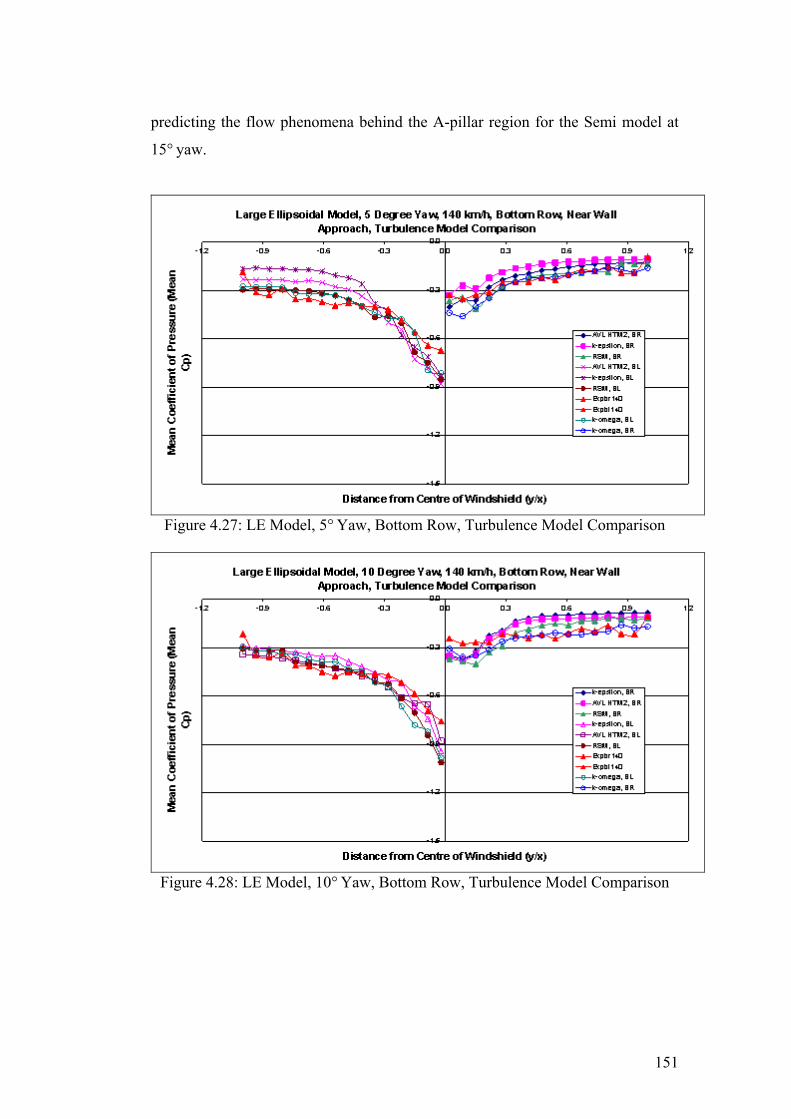
predicting the flow phenomena behind the A-pillar region for the Semi model at
15° yaw.
Figure 4.27: LE Model, 5° Yaw, Bottom Row, Turbulence Model Comparison
Figure 4.28: LE Model, 10° Yaw, Bottom Row, Turbulence Model Comparison
151
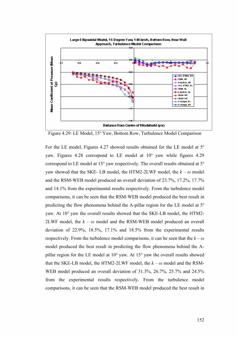
Figure 4.29: LE Model, 15° Yaw, Bottom Row, Turbulence Model Comparison
For the LE model, Figures 4.27 showed results obtained for the LE model at 5°
yaw. Figures 4.28 correspond to LE model at 10° yaw while figures 4.29
correspond to LE model at 15° yaw respectively. The overall results obtained at 5°
yaw showed that the SKE- LB model, the HTM2-2LWF model, the k – ω model
and the RSM-WEB model produced an overall deviation of 23.7%, 17.2%, 17.7%
and 14.1% from the experimental results respectively. From the turbulence model
comparisons, it can be seen that the RSM-WEB model produced the best result in
predicting the flow phenomena behind the A-pillar region for the LE model at 5°
yaw. At 10° yaw the overall results showed that the SKE-LB model, the HTM2-
2LWF model, the k – ω model and the RSM-WEB model produced an overall
deviation of 22.9%, 18.5%, 17.1% and 18.5% from the experimental results
respectively. From the turbulence model comparisons, it can be seen that the k – ω
model produced the best result in predicting the flow phenomena behind the A-
pillar region for the LE model at 10° yaw. At 15° yaw the overall results showed
that the SKE-LB model, the HTM2-2LWF model, the k – ω model and the RSM-
WEB model produced an overall deviation of 31.3%, 26.7%, 25.7% and 24.5%
from the experimental results respectively. From the turbulence model
comparisons, it can be seen that the RSM-WEB model produced the best result in
152

predicting the flow phenomena behind the A-pillar region for the LE model at 15°
yaw.
Figure 4.30: SE Model, 5° Yaw, Bottom Row, RSM-WEB Turbulence Model
Figure 4.31: SE Model, 10° Yaw, Bottom Row, RSM-WEB Turbulence Model
153

Figure 4.32: SE Model, 15° Yaw, Bottom Row, RSM-WEB Turbulence Model
From the comparative investigation conducted using the SE model, the RSM-
WEB model produced results with the minimum percentage error deviation. At 5º,
10° and 15° yaw, the percentage error of deviation are 16.8%, 18.8% and 20.3%
(Figure 4.30, 4.31, 4.32). For the Semi model, the RSM-WEB model produced
results with the minimum percentage error deviation. At 5°, 10° and 15° yaw, the
percentage error of deviation are 14.5%, 15.8% and 18.1% (Figure 4.33, 4.34,
4.35). Finally, for the LE model, the RSM-WEB model produced results with the
minimum percentage error deviation. At 5°, 10° and 15° yaw, the percentage error
of deviation are 14.1%, 18.5% and 24.5% (Figure 4.36, 4.37, 4.38). It can be
concluded that the RSM-WEB model is the most feasible near wall and turbulence
model combination for the circular models at yaw angles and will be used as the
CFD model for further analysis later in this chapter. The percentage error of
deviation for the RSM-WEB is within allowable values recommended, Swinburne
(2000).
154

Figure 4.33: Semi Model, 5° Yaw, Bottom Row, RSM-WEB Turbulence Model
Figure 4.34: Semi Model, 10° Yaw, Bottom Row, RSM-WEB Turbulence Model
155

Figure 4.35: Semi Model, 15° Yaw, Bottom Row, RSM-WEB Turbulence Model
From the study, it can be seen that the RSM-WEB model obtained improvement
over the eddy viscosity models in modelling the circular models at various yaw
angles due to better prediction of complex three dimensional flow that are
subjected to curved surfaces, swirl, rotation, rapid variation of strain rate and
boundary layer separation, FLUENT (2003), Wilcox (2002). These are
implemented by modelling Reynolds stresses via transport equations, by passing
the traditional method of the Eddy Viscosity method.
Figure 4.36: LE Model, 5° Yaw, Bottom Row, RSM-WEB Turbulence Model
156

Figure 4.37: LE Model, 10° Yaw, Bottom Row, RSM-WEB Turbulence Model
Figure 4.38: LE Model, 15° Yaw, Bottom Row, RSM-WEB Turbulence Model
157

4.2.4.3 Sharp Edge Models at 0°, 5°, 10° and 15º Yaw –
Near Wall Model and Turbulence Model
Feasibility Study
The sharp edge models investigated in this study are the SL and RE models at 0°,
5°, 10° and 15° yaw. Comparisons were first made against the experimental data
of Alam (2000) on the performance of the SL model at 0° yaw using various k – ε
turbulence models and near wall models and can be seen in Figures 4.39 and 4.40.
The k – ε model used was of the SKE-LB model, RNG and Realizable k – ε
models using the one equation near wall model of Wolfstein (1969). Comparisons
were conducted for the model at inlet free-stream velocity of 140 km/h. From the
figures, the Realizable model produced the least of error deviation at 55.6%, as
compared to 61.0% and 69.6% for the RNG and SKE-LB models respectively.
Taking the results obtained from the Realizable k – ε and comparing with
turbulence models of k – ω, HTM2-2LWF and RSM-WEB showed that the RSM-
WEB produced results with the least error deviation at 29.8%, followed by the k –
ω model at 35.8% and the AVL HTM2 at 54.1% (Figures 4.41 and 4.42). Figures
4.43 showed the Cp mean distribution behind the A-pillar region obtained from
the RSM-WEB turbulence model for the SL model at 5° yaw. The under
prediction of the relative Cp distribution produced on the combined bottom and
top row monitoring location yielded an average of 27.2%. Figures 4.44 showed
the Cp mean distribution behind the A-pillar region obtained from the RSM-WEB
turbulence model for the SL model at 10° yaw. The under prediction of the
relative Cp distribution produced on the combined bottom and top row monitoring
location yielded an average of 25.3%. Figures 4.45 showed the Cp mean
distribution behind the A-pillar region obtained from the RSM-WEB turbulence
model for the SL model at 15° yaw. The under prediction of the relative Cp
distribution produced on the combined bottom and top row monitoring location
yielded an average of 21.9%. The performance of the turbulence models are
consistent as what was reviewed and discussed in section 3.6.
158
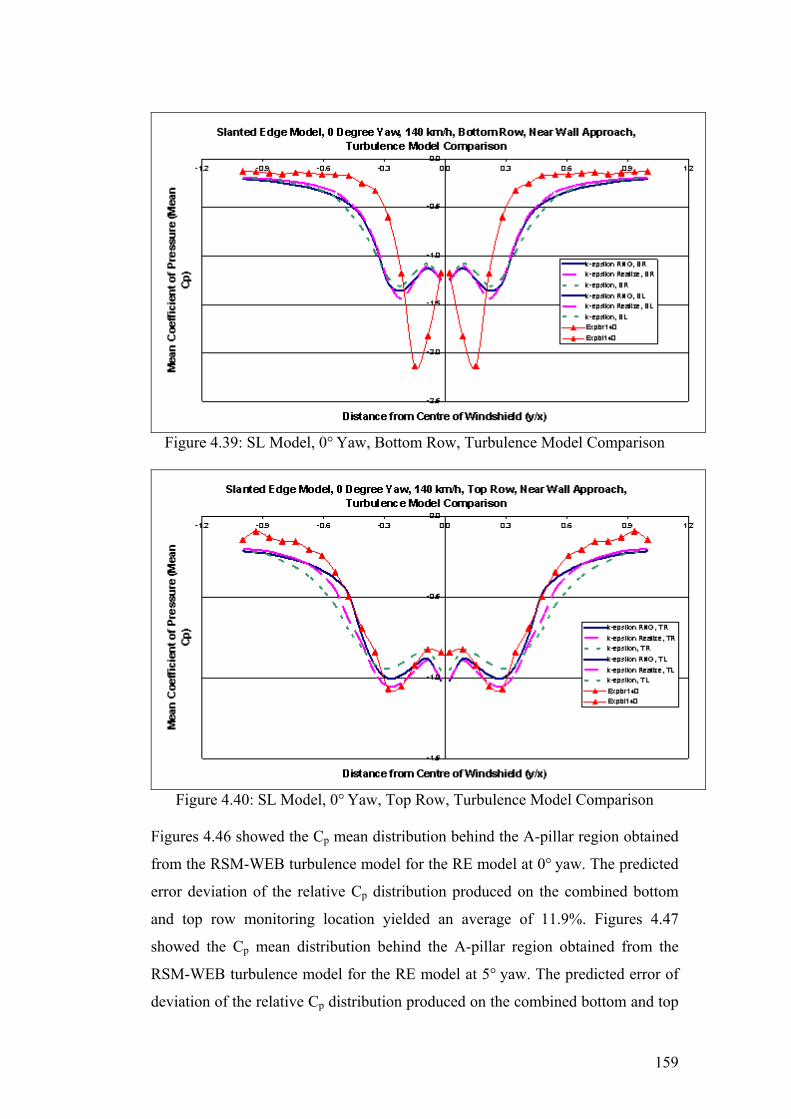
Figure 4.39: SL Model, 0° Yaw, Bottom Row, Turbulence Model Comparison
Figure 4.40: SL Model, 0° Yaw, Top Row, Turbulence Model Comparison
Figures 4.46 showed the Cp mean distribution behind the A-pillar region obtained
from the RSM-WEB turbulence model for the RE model at 0° yaw. The predicted
error deviation of the relative Cp distribution produced on the combined bottom
and top row monitoring location yielded an average of 11.9%. Figures 4.47
showed the Cp mean distribution behind the A-pillar region obtained from the
RSM-WEB turbulence model for the RE model at 5° yaw. The predicted error of
deviation of the relative Cp distribution produced on the combined bottom and top
159

row monitoring location yielded an average of 15.2%. Figures 4.48 showed the Cp
mean distribution behind the A-pillar region obtained from the RSM-WEB
turbulence model for the RE model at 10° yaw. The predicted error deviation of
the relative Cp distribution produced on the combined bottom and top row
monitoring location yielded an average of 21.1%. Figures 4.49 showed the Cp
mean distribution behind the A-pillar region obtained from the RSM-WEB
turbulence model for the RE model at 15° yaw. The predicted error deviation of
the relative Cp distribution produced on the combined bottom and top row
monitoring location yielded an average of 19.5%.
Figure 4.41: SL Model, 0° Yaw, Bottom Row, Turbulence Model Comparison
160
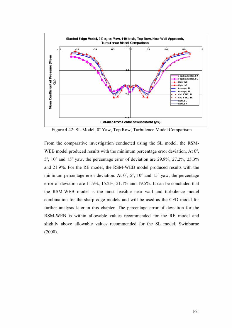
Figure 4.42: SL Model, 0° Yaw, Top Row, Turbulence Model Comparison
From the comparative investigation conducted using the SL model, the RSM-
WEB model produced results with the minimum percentage error deviation. At 0°,
5º, 10° and 15° yaw, the percentage error of deviation are 29.8%, 27.2%, 25.3%
and 21.9%. For the RE model, the RSM-WEB model produced results with the
minimum percentage error deviation. At 0°, 5°, 10° and 15° yaw, the percentage
error of deviation are 11.9%, 15.2%, 21.1% and 19.5%. It can be concluded that
the RSM-WEB model is the most feasible near wall and turbulence model
combination for the sharp edge models and will be used as the CFD model for
further analysis later in this chapter. The percentage error of deviation for the
RSM-WEB is within allowable values recommended for the RE model and
slightly above allowable values recommended for the SL model, Swinburne
(2000).
161

Figure 4.43: Slanted Edge Model, 5° Yaw, Bottom Row, RSM-WEB Turbulence
Model
Figure 4.44: Slanted Edge Model, 10° Yaw, Bottom Row, RSM-WEB Turbulence
Model
162

Figure 4.45: Slanted Edge Model, 15° Yaw, Bottom Row, RSM-WEB Turbulence
Model
Figure 4.46: Rectangular Model, 0° Yaw, Bottom Row, RSM-WEB Turbulence
Model
163

Figure 4.47: Rectangular Model, 5° Yaw, Bottom Row, RSM-WEB Turbulence
Model
Figure 4.48: Rectangular Model, 10° Yaw, Bottom Row, RSM-WEB Turbulence
Model
164

Figure 4.49: Rectangular Model, 15° Yaw, Bottom Row, RSM-WEB Turbulence
Model
4.3 Circular Models at 0º Yaw – Results and Discussion
CFD results obtained from the SKE-2LWF model were presented as external
airflow streamline in Figures 4.50 and 4.51. The flow behaviour was in agreement
with Barnard (1996). It can be seen that the airflow movement around the vehicle
starts from the junction of the A-pillar base. The circular apex of the A-pillar
causes separation, which was similar to a trailing edge separation (Figures 1.2 and
1.3; page 5 and 7). This resulted in the formation of boundary layer close to the
vehicle wall surface. The boundary layer thickness increase as the airflow
progressed downstream. The formation of turbulent boundary layer originated in
laminar form and the laminar effect causes airflow to slide over each other due to
skin friction drag formed with the vehicle wall surface. This will cause the outer
air layer moving faster than the inner one which will slow down the flow, causing
boundary layer to gradually become thicker. As the formation of turbulent
boundary layer progressed, the flow becomes streamlined, following the contours
of the vehicle body. The small scale turbulent eddies are causing rapid mixing.
However, very close to the surface within a turbulent boundary layer flow, a thin
sub layer of laminar flow still exists (Figure 4.52, page 167). This result in a
gradual increase in relative pressure as the airflow moves downstream, which will
have a direct impact on the process of turbulent mixing. It will allow energy
165

transfer to take place from the fast moving eddies to the slower moving eddies in
the turbulent boundary layer resulting in turbulent boundary layer with low
turbulent activity.
Roof Junction
Figure 4.50: SE Model, 0° Yaw, External Surface Streamline, Front View
A-pillar Base Junction
A-pillar Apex
2-D turbulent boundary layer ‘separation bubble’
Figure 4.51: SE Model, 0° Yaw, External Surface Streamline, Top View
166

The turbulent boundary layer exists in a quasi two-dimensional form. This can be
seen from the velocity vector generated in Figure 4.53. Measurement of the cross
section indicate a horizontal and vertical separation of 115-mm and 102-mm.
Comparison against Semi and LE model showed no significant difference in
either the shape and form of the separation. Correlation between surface
streamline flow of the model and the streamline visualization using wool tuffs by
Alam (2000) showed that the turbulent boundary layer close to the surface is
attached and quasi two-dimensional (Figures 4.54 and 4.55). The quasi two-
dimensional separation that was observed was in agreement with Hucho (1998). It
can be seen from the Figures that the quasi two-dimensional type flow separates at
the A-pillar apex running and almost perpendicular to the local direction of flow.
The separation causes vortices to roll up with their axes almost parallel to the
separation line forming a circular and elongated quasi two-dimensional separation
downstream to the flow. Turbulent mixing dissipates most of their kinetic energy
making their development as continuing free trailing vortices, often weak and
even untraceable. Often, two-dimensional separation forms a continuing trailing
vortex with three-dimensional separation forms a cone shaped helical vortex.
Correlation in Figure 4.18 against Alam (2000) showed that Cp distribution at
various distance along the A-pillar/side wall was Reynolds number independent
and that most importantly, flow separation exists during the start of the flow,
growing weaker as it moves downstream.
167

Laminar Flow close to surface
Figure 4.52: SE Model, 0° Yaw, Top View, Turbulent Velocity
Vertical Component
Horizontal Component
Figure 4.53: SE Model, 0° Yaw, Front View, Velocity Vector
Furthermore from Figure 4.51, the quasi two-dimensional turbulent boundary
layer separation forms a region defined as ‘separation bubble’, Hucho (1998).
168

Separation bubble is defined as the region between flow separation and
reattachment caused by adverse pressure gradient from the rapid change of
pressure at the A-pillar apex. The separation bubble region will form region of
vortex circulation termed the ‘dead water’ zone. According to Watanabe et al.
(1978), the vortex development forms region of low relative pressure and that the
core is located at the vortex core of the separation. This is in agreement with
Figure 4.18 where region of low relative pressure was observed occurring at the
vortex core located at the apex of the A-pillar. Observation from the Semi and LE
models in Figures 4.56 and 4.57showed similar magnitude and pattern of
distribution for turbulent velocity as compared with the SE model (Figure 4.52).
However, observation seen from Figures 4.18 to 4.20 showed a decrease in Cp as
the windshield radii of the models increases. This is in agreement with Callister et
al. (1998). An alternative way of reducing A-pillar vortex size and intensity was
to increase the surface area of the models by increasing the windshield/A-pillar
radius.
A-pillar apex attached turbulent region
A-pillar base junction separated turbulent region
5° vortex core axis relative to the horizontal axis
Figure 4.54: SE Model, 0° Yaw, Surface Streamline
169

Similar Flow Pattern as CFD model
Figure 4.55: SE Model at 0° Yaw, Surface Streamline Visualisation using Wool
Tuffs (after Alam, 2000)
Figure 4.56: Semi Model, 0° Yaw, Top View, Turbulent Velocity
170

Figure 4.57: LE Model, 0° Yaw, Top View, Turbulent Velocity
4.4 Circular Models at 5° yaw – Results and Discussion
The surface flow streamline for the SE, Semi and LE model at 5° yaw can be seen
in Figures 4.58 to 4.61. It can be seen from these figures that the effect of yaw
angle is creating bigger separation regions around and behind the A-pillar in the
leeward region as oppose to the windward region of the flow. This observation is
in agreement with Alam et al. (1998), Bearman et al. (1989) and Haruna et al.
(1990). The presence of yaw angle resulted in a larger separation on the leeward
side due to an increased in turbulence intensity (Figures 4.62 and 4.63). Figures
4.62 and 4.63 of the velocity vector and turbulent velocity show a larger
separation in the leeward region at 5° yaw. Measurement of the cross section
indicate a horizontal and vertical separation of 150-mm and 370-mm. Observation
against Semi and LE model showed no significant difference in either the shape
and form of the separation. However, comparing Cp coefficient between the SE,
Semi and LE model do show a decrease in negative relative pressure magnitude,
which translate in a decline in turbulence intensity as the windshield radii
increases (Figures 4.30, 4.33 and 4.36, page 152 to 155).
171
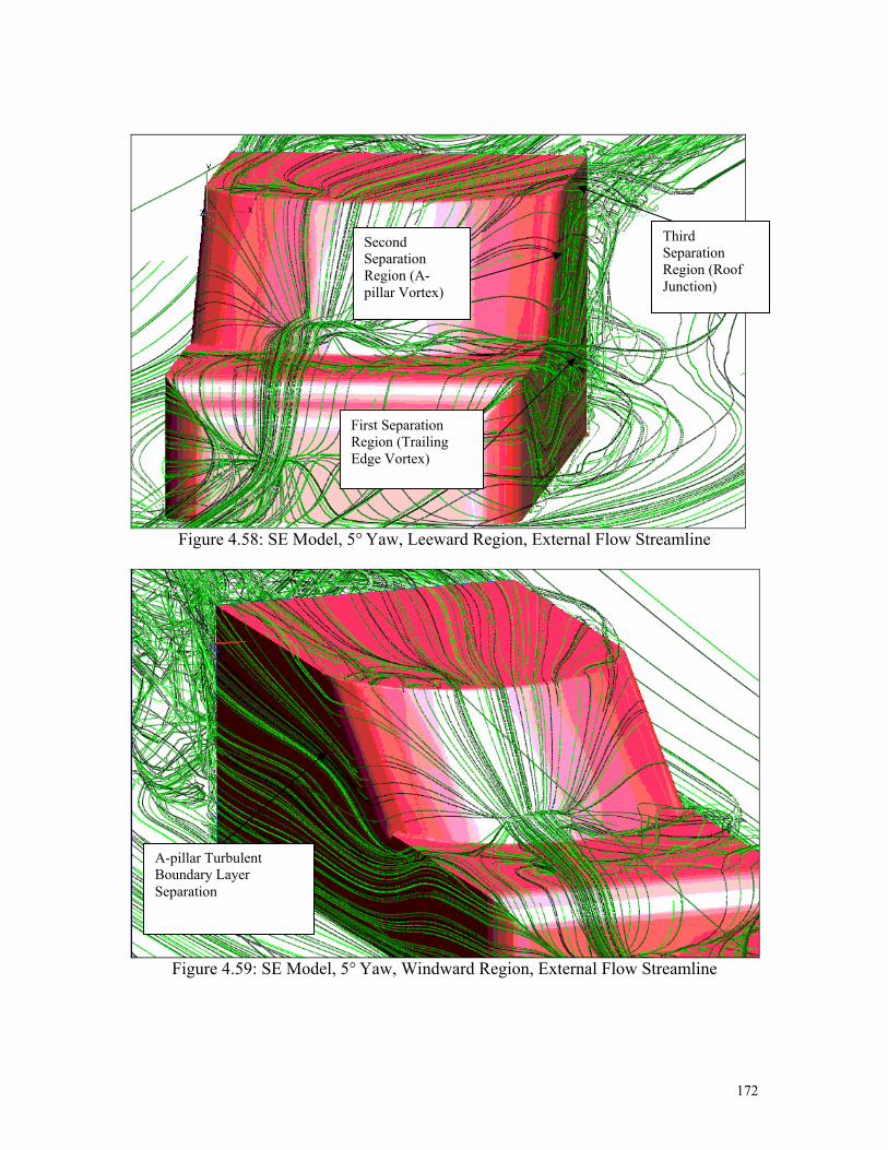
Third Separation Region (Roof Junction)
Second Separation Region (A-pillar Vortex)
First Separation Region (Trailing Edge Vortex)
Figure 4.58: SE Model, 5° Yaw, Leeward Region, External Flow Streamline
A-pillar Turbulent Boundary Layer Separation
Figure 4.59: SE Model, 5° Yaw, Windward Region, External Flow Streamline
172

It was observed from the surface flow streamline for each model that the source of flow
separation in the leeward region originated from the corner of the windshield/A-pillar
junction, the A-pillar apex and from the roof junction of the model. This observation was
in agreement with Hanaoka et al. (1993), Ahmed (1998) and Zhu et al. (1993, 1994) in
which it was noted that the regions of separated flow on a vehicle occur on the A-pillar
base, together with the front side window and roof junction behind the A-pillar.
Trailing Edge Separation
A-pillar Separation
Figure 4.60: Semi Model, 5° Yaw, Front View, External Flow Streamline
It can also be seen in Figures 4.58 to 4.61, that in the windward side of the flow, the
airflow originated from impingement on the model windshield, re-directing the flow to
the windward side of the model. The induced air flow creates an attached turbulent
boundary layer region as it moves around the curvature of the windshield in the A-pillar
region downstream to the flow. The airflow flowing around the A-pillar region was
observed spilling over the windward roof junction as attached flow.
The flow separation occurring in the leeward region was a combination of two-
dimensional and three-dimensional, while the flow separation occurring in the windward
region was mainly two-dimensional. It was observed from Figures 4.58 to 4.61 in the
173

leeward region that the separation region originated from the A-pillar base junction was
quasi two dimensional. This was in agreement with Hucho (1998) in which he stated that
the separation causes vortices to roll up with their axes almost parallel to the separation
line. Turbulent mixing dissipates most of their kinetic energy making their development
as continuing free trailing vortices.
Larger trailing edge separation region
Figure 4.61: LE Model, 5° Yaw, Front View, Surface Streamline
The separation from the A-pillar apex in the leeward region was observed as three-
dimensional, a mixture of separated and attached flow. The mixture of separation and
attached flow behind the A-pillar region was attributed to the yaw angle of the vehicle.
This was in agreement with Barnard (1996). Strong sideways or cross-stream components
on the surface of a vehicle complicate the formation and behaviour of the boundary layer.
Cross-stream components are more inclined to cause early transition of the turbulent
boundary layer. Cross-stream flows can also keep the boundary layer attached by
reducing high-pressure flow, making the pressure gradient less adverse. The separated
region exhibit rotational flow while the attached region remains irrotational, Haruna et al
(1990). The three dimensional separation normally occurs due to the effect of the
174
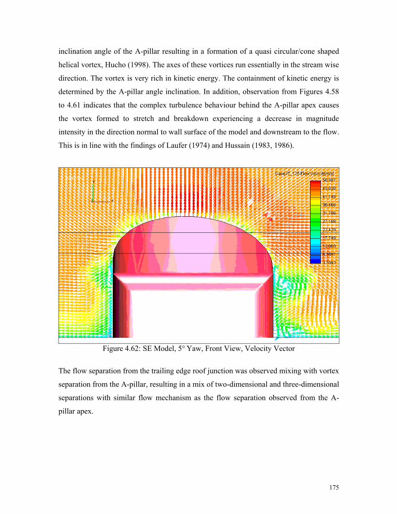
inclination angle of the A-pillar resulting in a formation of a quasi circular/cone shaped
helical vortex, Hucho (1998). The axes of these vortices run essentially in the stream wise
direction. The vortex is very rich in kinetic energy. The containment of kinetic energy is
determined by the A-pillar angle inclination. In addition, observation from Figures 4.58
to 4.61 indicates that the complex turbulence behaviour behind the A-pillar apex causes
the vortex formed to stretch and breakdown experiencing a decrease in magnitude
intensity in the direction normal to wall surface of the model and downstream to the flow.
This is in line with the findings of Laufer (1974) and Hussain (1983, 1986).
Figure 4.62: SE Model, 5° Yaw, Front View, Velocity Vector
The flow separation from the trailing edge roof junction was observed mixing with vortex
separation from the A-pillar, resulting in a mix of two-dimensional and three-dimensional
separations with similar flow mechanism as the flow separation observed from the A-
pillar apex.
175

A-pillar apex separated flow
Trailing edge separation from A-pillar base junction
Figure 4.63: SE Model, 5° Yaw, Top View, Turbulent Velocity
Inspection from Figure 4.64 showed that the anisotropic nature of the turbulent flow
behind the A-pillar region. The Reynolds stresses component distribution revealed
different distribution in the UU (horizontal), VV (vertical) and WW (downstream)
component, which disproves the usage of Boussinesq assumption in the eddy viscosity
models in assuming isotropic turbulence, Wilcox (2002). The distribution of the
Reynolds stresses components along the surface of the wall revealed the stream wise UU
Reynolds stress component is around 52.3% of the total turbulent kinetic energy
distribution. This is within close agreement to 60% for turbulent boundary layer
distribution, Imperial College (circa. 1980s). The Reynolds stresses component also
showed that along the surface of the wall, the leeward region of the flow displayed a
higher Reynolds stresses intensity. This was due to the yawing orientation of the model
that produces a higher Reynolds stresses component due to the vortex generation in the
leeward side of the flow as compared to the windward side. The complex three-
dimensional nature of the flow also revealed that the VV Reynolds stress component
having a higher intensity compared to the WW Reynolds stress component as what was
observed by Nienaltowska (1993) and in the standard free shear and flat plate turbulent
176

boundary layer flow, Imperial College (circa. 1980s). The Reynolds stresses distributions
on the windward region were 37.0% higher compared to the distribution in the leeward
region.
Leeward Region
Figure 4.64: SE Model, 5º Yaw, Reynolds Stresses Component, Leeward and Windward
Region of the A-pillar
177

4.5 Circular Models at 10° and 15° Yaw – Results and
Discussion
The surface flow streamline for the SE, Semi and LE model at 10° and 15° yaw can be
seen in Figures 4.65 to 4.70. When comparing these figures to those at yaw angles of 0°
and 5° respectively, it was observed that the effect of yaw angle above 10° underwent a
sudden escalation in separation regions and turbulence intensity around and behind the A-
pillar in the leeward and windward region of the flow respectively. This observation is in
agreement with Bearman et al. (1989). At yaw angle of 10° the separation originated from
the A-pillar base junction and the A-pillar apex are subjected to higher adverse pressure
gradient. Stronger sideways or cross-stream flows are present causing a much earlier
transition of the turbulent boundary layer. As a result, larger area of separation and
recirculation generated due to the higher yaw angle airflow approach. Region of low
pressure close to the wall surface was present due to activities occurring beneath the
turbulence boundary layer. The airflow surrounding the A-pillar region will be highly
rotational and the vortex generated is high in kinetic energy. The highly turbulent nature
will cause the vortex transient behaviour to fluctuate in size due to the act of mixing and
dissipation of turbulent eddies. The size fluctuation will cause the vortex to periodically
stretch and breakdown due to fluctuation in magnitude intensity in the direction normal to
wall surface of the model and downstream to the flow. This is in line with the findings of
Laufer (1974) and Hussain (1983, 1986).
178

Combination of roof junction and A-pillar apex separated flow
Trailing edge separation from A-pillar base junction
Figure 4.65: SE Model, 10° Yaw, Front View, External Flow Streamline
3-D A-pillar apex vortex flow
2-D free trailing edge vortex from A-pillar base junction
Figure 4.66: SE Model, 15° Yaw, Leeward View, External Flow Streamline
As with observations at 5° yaw, it was observed from the surface flow streamline for each
model at 10° and 15° yaw that the source of flow separation in the leeward region
originated from the corner of the A-pillar base junction, the A-pillar apex and from the
179

roof junction of the model. The vortex generated from the A-pillar base junction formed a
trailing helical shaped vortex while vortex generated from the A-pillar apex formed a
combination of quasi elongated circular and cone helical vortex. The vortex generated
from the roof junction formed a trailing circular shape vortex, exhibiting rotation and
circulation flowing in stream wise direction. It can be seen from Figures 4.65 to 4.70 that
the direction of flow generated by all three vortex sources interferes with each other
creating a chaotic turbulent structure.
A-pillar Separation
Trailing Edge Separation
Figure 4.67: Semi Model, 10° Yaw, Front View, External Flow Streamline
It can also be seen in Figures 4.65 to 4.70, in the windward side of the flow, the airflow
impinges on the model windshield, re-directing the flow to the windward side of the
model. The induced air flow creates an attached turbulent boundary layer region as it
moves around the curvature of the windshield in the A-pillar region downstream to the
flow. The airflow flowing around the A-pillar region was also observed spilling over the
windward roof junction as attached flow. At 10° and 15° yaw, the over spilling at the roof
junction is higher forming a leading edge vortex circulating cross wise almost halfway
across the roof.
180

Trailing edge separation region
Figure 4.68: LE Model, 10° Yaw, Front View, Surface Streamline
In addition, Figures 4.75 to 4.78 of the turbulence velocity and velocity vector slice also
shows a larger separation in the leeward region at 10° and 15° yaw. Observation against
the SE, Semi and LE models showed no significant difference in both the shape and the
mechanism of the separation (Figure 4.65 to 4.70). However, similar with the observation
at 5° yaw, comparing Cp coefficient between the SE, Semi and LE model do show a
decrease in negative relative pressure magnitude, which translate in a decline in
turbulence intensity as the windshield radii increases. Measurement of the separation
cross section for the model at 10° indicate a horizontal and vertical separation of 214-mm
and 404-mm. Measurement of the separation cross section for the model at 15° indicate a
horizontal and vertical separation of 340-mm and 430-mm. Correlation between surface
streamline flow of the model and the streamline visualization using wool tuffs by Alam
(2000) showed that the turbulent boundary layer close to the surface is attached and quasi
two-dimensional (Figures 4.71 to 4.74).
181

Trailing Edge Separation
A-pillar Separation
Figure 4.69: Semi Model, 15° Yaw, Front View, External Flow Streamline
Trailing edge separation
Figure 4.70: LE Model, 15° Yaw, Front View, Surface Streamline
The axis of the vortex core with respect to the horizontal plane was observed to increase
as the yaw angle increases (Figures 4.54; page 168, 4.71; page 182 and 4.73; page 183).
Axis of the vortex core for model subjected to 0° yaw was observed to be at 5° from the
182

horizontal plane. At the leeward region when subjected to 15° yaw, the vortex core axis
was measured at an angle of 10° from the horizontal plane. At the windward region when
subjected to 15° yaw, the vortex core axis was measured at an angle 20° respectively from
the horizontal plane.
Reattachment Region
10° vortex core axis relative to the horizontal axis
Figure 4.71: SE Model, 15° Yaw, Leeward View, Surface Flow Streamline
Similar Flow Pattern as CFD model
Figure 4.72: SE Model at 15° Yaw in the Leeward Region, Surface Streamline Visualisation using Wool Tuffs (after Alam, 2000)
183
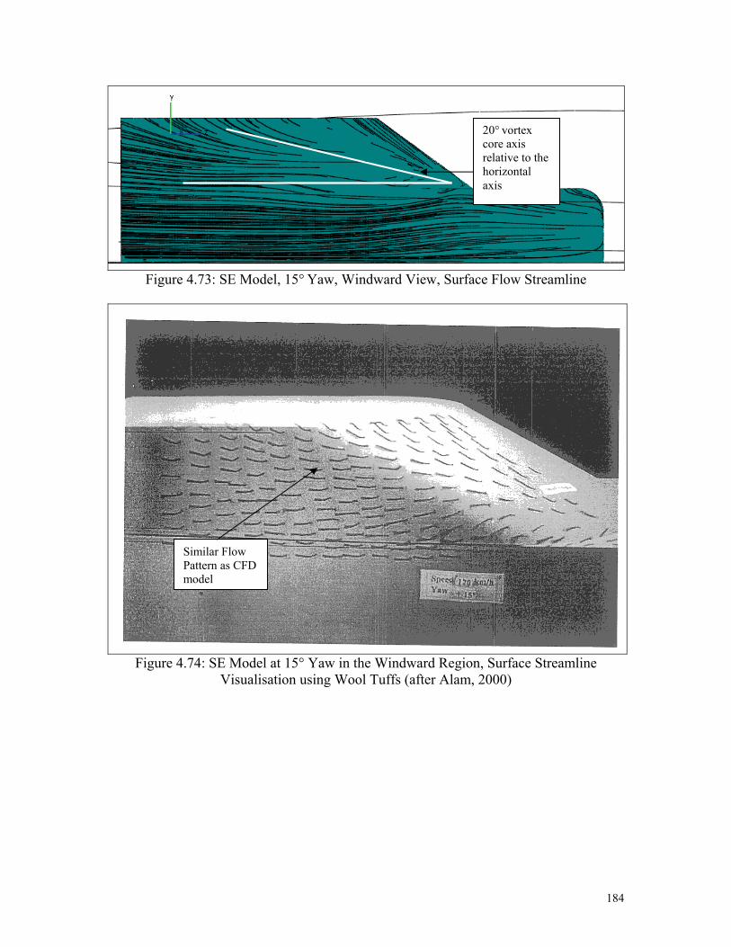
Figure 4.73: SE Model, 15° Yaw, Windward View, Surface Flow Streamline
20° vortex core axis relative to the horizontal axis
Similar Flow Pattern as CFD model
Figure 4.74: SE Model at 15° Yaw in the Windward Region, Surface Streamline Visualisation using Wool Tuffs (after Alam, 2000)
184

A-pillar apex separated flow
Trailing edge separation from A-pillar base junction
Figure 4.75: SE Model, 10° Yaw, Top View, Turbulent Velocity
Figure 4.76: SE Model, 10° Yaw, Front View, Velocity Vector
185

Figure 4.77: SE Model, 15° Yaw, Top View, Turbulent Velocity
Figure 4.78: SE Model, 15° Yaw, Front View, Velocity Vector
Inspection from Figures 4.79 and 4.80 reveal the distribution of Reynolds stresses
component were different in the UU, VV and WW component behind the A-pillar region.
186

Inspection from Figure 4.79 showed Reynolds stress component distribution at 10° yaw.
Comparison to the distribution at 5° yaw showed several differences, which further show
the anisotropic nature of the turbulent flow behind the A-pillar region. In the leeward
region, the UU and VV component showed an increase production of turbulent kinetic
energy and dissipation rate close to the wall surface region within the separation region.
In the windward region, the Reynolds stress in the UU component showed a significant
increase in comparison to the other component, which reflect on the fact that the flow in
the windward region was predominantly attached, and moving in the stream wise
direction, downstream to the flow. The stream wise UU Reynolds stress component is
around 50.3% of the total turbulent kinetic energy distribution. This is within close
agreement to 60% for turbulent boundary layer distribution along a flat plate, Imperial
College (circa. 1980s). The Reynolds stresses distributions on the windward region were
35.0% higher compared to the distribution in the leeward region.
Figure 4.79: SE Model, 10º Yaw, Reynolds Stresses Component, Leeward and Windward
Region of the A-pillar
Inspection from Figures 4.80 showed Reynolds stress component distribution at 15° yaw.
The stream wise UU Reynolds stress component is around 52.8% of the total turbulent
187

kinetic energy distribution. This is within close agreement to 60% for turbulent boundary
layer distribution along a flat plate, Imperial College (circa. 1980s). The Reynolds
stresses distributions on the windward region were 37.0% higher compared to the
distribution in the leeward region.
Figure 4.80: SE Model, 15º Yaw, Reynolds Stresses Component, Leeward and Windward
Region of the A-pillar
188

4.6 RE Model at 0° Yaw – Results and Discussion
CFD results obtained for the RE model at 0° yaw from the RSM-WEB model was
presented as external airflow streamline in Figures 4.81. The airflow movement around
the vehicle starts from vehicle windshield and separates from the A-pillar base junction,
A-pillar edge and the roof junction.
Roof Junction separation
Trailing Edge Separation
A-pillar Separation
Figure 4.81: Rectangular Model, 0° Yaw, Front View, External Flow Streamline
The roof junction separation was similar to a trailing edge separation observed in the
circular models. Separation from the roof junction formed a quasi two-dimensional flow
resulted from the generation of adverse pressure gradient due to the rapid change in
pressure. The separation at the roof junction causes vortices to roll up with their axes
almost parallel to the separation line forming a continuing and trailing two dimensional
vortex downstream to the flow. Turbulent mixing dissipates most of their kinetic energy
making their development often weak and even untraceable, Hucho (1998).
189

The A-pillar edge separation formed a quasi two-dimensional separation bubble region,
Hucho (1998). The rapid change of pressure at the A-pillar edge causes formation of
adverse pressure gradient between the region of flow separation and reattachment. This
will also result in a dead water vortex circulation zone formation downstream to the flow.
According to Watanabe et al. (1978), the separation bubble forms region of low relative
pressure in which the core is located at the vortex core of the separation.
Figure 4.82: Rectangular Model, 0° Yaw, Side View, Surface Streamline
55° vortex core axis relative to the horizontal axis
Similar Flow Pattern as CFD model
Figure 4.83: RE Model at 0° Yaw, Surface Streamline Visualisation using Wool Tuffs (after Alam, 2000)
190
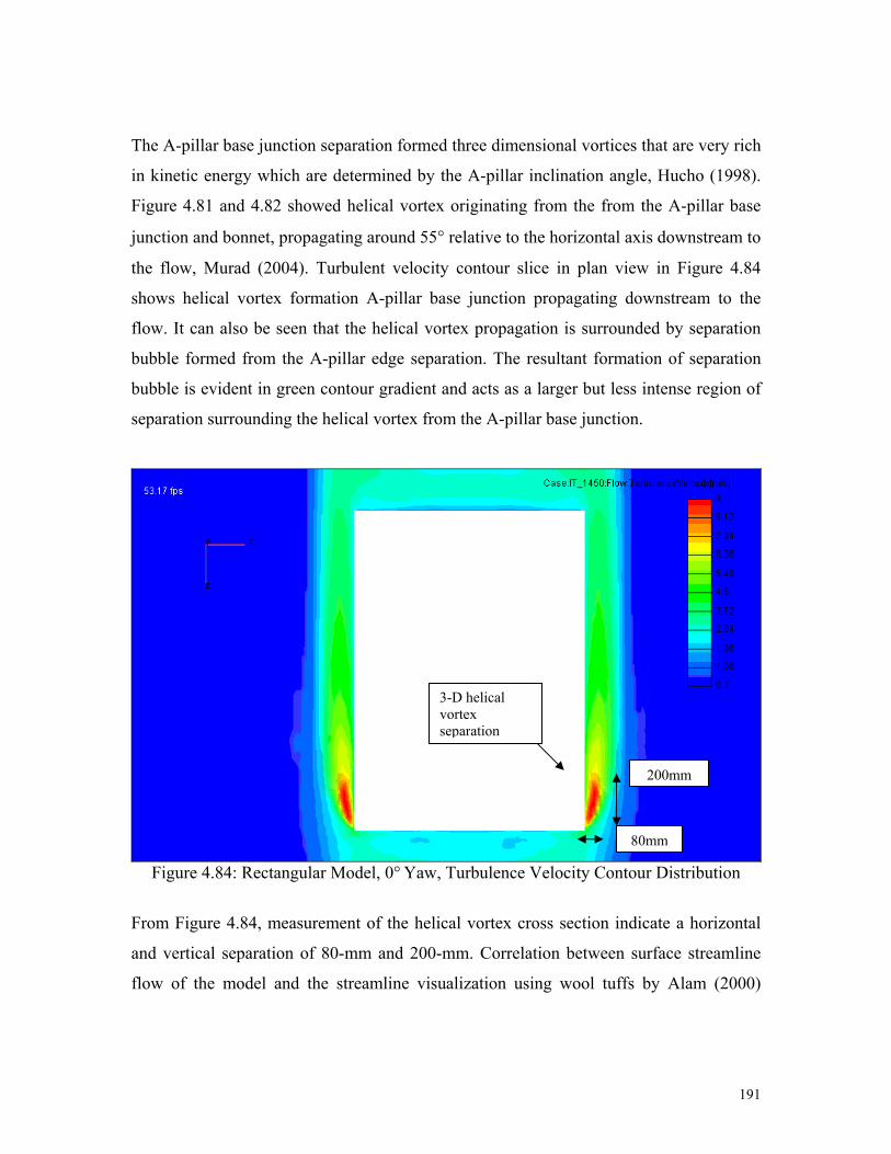
The A-pillar base junction separation formed three dimensional vortices that are very rich
in kinetic energy which are determined by the A-pillar inclination angle, Hucho (1998).
Figure 4.81 and 4.82 showed helical vortex originating from the from the A-pillar base
junction and bonnet, propagating around 55° relative to the horizontal axis downstream to
the flow, Murad (2004). Turbulent velocity contour slice in plan view in Figure 4.84
shows helical vortex formation A-pillar base junction propagating downstream to the
flow. It can also be seen that the helical vortex propagation is surrounded by separation
bubble formed from the A-pillar edge separation. The resultant formation of separation
bubble is evident in green contour gradient and acts as a larger but less intense region of
separation surrounding the helical vortex from the A-pillar base junction.
3-D helical vortex separation
200mm
80mm
Figure 4.84: Rectangular Model, 0° Yaw, Turbulence Velocity Contour Distribution
From Figure 4.84, measurement of the helical vortex cross section indicate a horizontal
and vertical separation of 80-mm and 200-mm. Correlation between surface streamline
flow of the model and the streamline visualization using wool tuffs by Alam (2000)
191
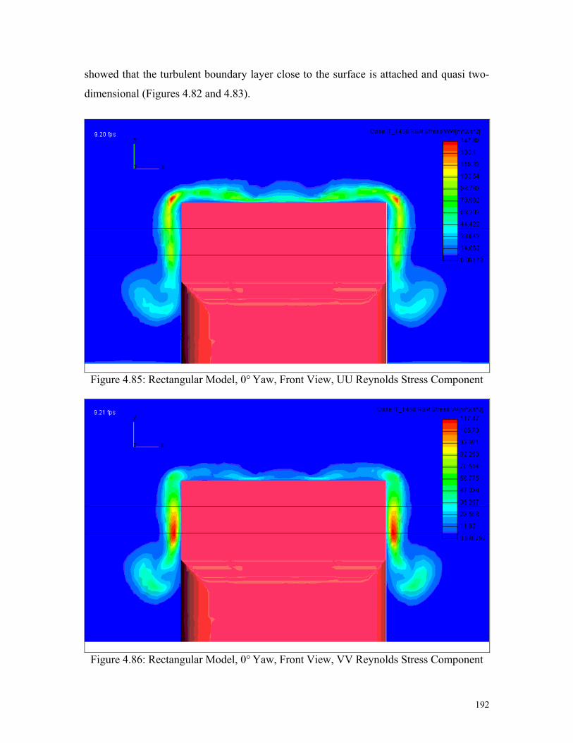
showed that the turbulent boundary layer close to the surface is attached and quasi two-
dimensional (Figures 4.82 and 4.83).
Figure 4.85: Rectangular Model, 0° Yaw, Front View, UU Reynolds Stress Component
Figure 4.86: Rectangular Model, 0° Yaw, Front View, VV Reynolds Stress Component
192

Figure 4.87: Rectangular Model, 0° Yaw, Front View, WW Reynolds Stress Component
Inspection from Figures 4.85 to 4.87 showed that the anisotropic nature of the turbulent
flow behind the A-pillar region. The Reynolds stresses component distribution revealed
different distribution in the UU, VV and WW component. Inspection from Figures
showed that the UU has the highest Reynolds stresses component distribution followed
by the VV and WW component respectively. This is within close agreement to the
circular models seen in previous sections and also with published literature (Imperial
College, circa. 1980s).
4.7 SL Model at 0° Yaw – Results and Discussion CFD results obtained for the SL model from the RSM-WEB model was presented as
external airflow streamline in Figure 4.88. The airflow movement around the SL model
starts from vehicle windshield experienced separation at the A-pillar region, in which
components consists of the A-pillar base junction, A-pillar edge and the roof junction.
193
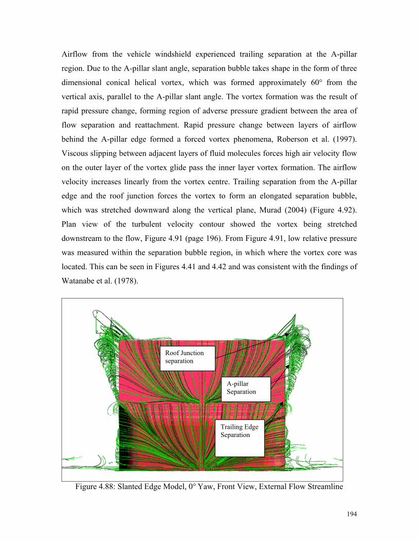
Airflow from the vehicle windshield experienced trailing separation at the A-pillar
region. Due to the A-pillar slant angle, separation bubble takes shape in the form of three
dimensional conical helical vortex, which was formed approximately 60° from the
vertical axis, parallel to the A-pillar slant angle. The vortex formation was the result of
rapid pressure change, forming region of adverse pressure gradient between the area of
flow separation and reattachment. Rapid pressure change between layers of airflow
behind the A-pillar edge formed a forced vortex phenomena, Roberson et al. (1997).
Viscous slipping between adjacent layers of fluid molecules forces high air velocity flow
on the outer layer of the vortex glide pass the inner layer vortex formation. The airflow
velocity increases linearly from the vortex centre. Trailing separation from the A-pillar
edge and the roof junction forces the vortex to form an elongated separation bubble,
which was stretched downward along the vertical plane, Murad (2004) (Figure 4.92).
Plan view of the turbulent velocity contour showed the vortex being stretched
downstream to the flow, Figure 4.91 (page 196). From Figure 4.91, low relative pressure
was measured within the separation bubble region, in which where the vortex core was
located. This can be seen in Figures 4.41 and 4.42 and was consistent with the findings of
Watanabe et al. (1978).
A-pillar Separation
Roof Junction separation
Trailing Edge Separation
Figure 4.88: Slanted Edge Model, 0° Yaw, Front View, External Flow Streamline
194

Measurements of the helical vortex cross section indicate a horizontal and vertical
separation of 113-mm and 274-mm. The vortex generated from the A-pillar base
junction, A-pillar apex and the roof junction combined to form a three-dimensional
helical vertical elongated cone shaped vortex. The combination of these three vortex
source creates a highly incensed turbulent structure propagating downstream to the flow.
Figure 4.89 showed that the helical vortex originating from the A-pillar base junction and
bonnet, propagates around 30° relative to the horizontal axis downstream to the flow,
Murad (2004). Correlation between surface streamline flow of the model and the
streamline visualization using wool tuffs by Alam (2000) showed that the turbulent
boundary layer close to the surface follows the same flow pattern as the separation
vortex, as shown in Figures 4.89 and 4.90. Region of vortex reattachment can be seen
halfway between the A-pillar edge and the A-pillar base junction. Correlation in Figures
4.40 and 4.41 (page 158 and 159) against Alam (2000) showed that Cp distribution at
various distance along the A-pillar/side wall was Reynolds number independent and that
most importantly, flow separation exists during the start of the flow, growing weaker as it
moves downstream.
30° vortex core axis relative to the horizontal axis
Figure 4.89: Slanted Edge Model, 0° Yaw, Side View, Surface Flow Streamline
195

Similar Flow Pattern as CFD model
Figure 4.90: SL Model at 0° Yaw, Surface Streamline Visualisation using Wool Tuffs (after Alam, 2000)
Low Relative Pressure Region
Figure 4.91: Slanted Edge Model, 0° Yaw, Turbulence Velocity Contour Distribution
196

Vertical helical cone shape vortex elongation
Figure 4.92: Slanted Edge Model, 0° Yaw, Front Plane View, Velocity Vector Distribution
Inspection from Figures 4.93 to 4.95 showed that the anisotropic nature of the turbulent
flow behind the A-pillar region. The Reynolds stresses component distribution revealed
different distribution in the UU, VV and WW component. Inspection from Figures
showed that the VV (vertical) has the highest Reynolds stresses component distribution
followed by the UU (horizontal) and WW (downstream) component respectively.
197

Figure 4.93: Slanted Edge Model, 0° Yaw, Front View, UU Reynolds Stress Component
Figure 4.94: Slanted Edge Model, 0° Yaw, Front View, VV Reynolds Stress Component
198

Figure 4.95: Slanted Edge Model, 0° Yaw, Front View, WW Reynolds Stress Component
4.8 RE Model at 5°, 10° and 15° Yaw – Results and Discussion
External surface streamline airflow observed for the Rectangular model at 5° yaw shows
flow separation both at the leeward and windward region of the A-pillar (Figure 4.96).
The 5° yaw causes the airflow to impinge slightly off centre on the windshield surface.
Trailing edge separation was observed originating from the junction of the A-pillar base,
the A-pillar edge and the roof junction. Quasi two-dimensional flow separation was
observed from the A-pillar base junction while a combination of two-dimensional and
three-dimensional flow separation was observed coming from the A-pillar apex and roof
junction. The perpendicular angle between the bonnet and windshield, also the
windshield and the roof causes quasi two-dimensional type flow to separate on the edge
and run perpendicular to the local direction of flow and interfering with each other
creating a chaotic turbulent structure. The separation causes vortices to roll up with their
axes almost parallel to the separation line. This was particularly evident at the A-pillar
edge and roof junction. Coupled with the yaw angle, the separation causes turbulent
199

mixing, which translate to a larger separation bubble and enhanced turbulent intensity
(Figure 4.99). Kinetic energy generated from the separation then dissipates downstream
as continuing free trailing vortices, Hucho (1998). The overall separation bubble, which
was a result of the chaotic turbulent structure, takes the form of a quasi circular elongated
separation vortex stretched downstream to the flow. The physical shape of the vortex for
the RE model at yaw angles are similar to those of the circular models. However, the
turbulent intensity are higher in the RE model due to the influence of the sharp A-pillar
edge as compared to the streamlines curved A-pillar in the circular models.
Measurements of the separation bubble in the leeward region indicate a cross and vertical
separation of 162-mm and 487-mm. Measurement in the windward region indicate a
cross and vertical separation of 44-mm and 267-mm.
A-pillar Separation
Roof Junction separation
Trailing Edge Separation
Figure 4.96: Rectangular Model, 5° Yaw, Frontal External Streamline Airflow
200

Figure 4.97: Rectangular Model, 10° Yaw, Frontal External Streamline Airflow
In the windward region of the A-pillar, the effect of the yaw angle, together with the
vertical windshield plane (Popat, 1991 and Hucho, 1998) causes the flow separation
bubble to be smaller but higher in turbulence intensity compared to the separation
occurring in the leeward region (Figures 4.96 and 4.47). The effect of the yaw angle and
the vertical windshield plane in the windward region forces the airflow to separate at the
edge of the A-pillar, having a smaller region of separation, recirculation and reattachment
thus generating high concentration of quasi two-dimensional turbulent flow mixing,
Murad (2004).
201

Figure 4.98: Rectangular Model, 15° Yaw, Frontal External Streamline Airflow
2-D and 3-D roof and A-pillar apex vortices
2-D trailing A-pillar base junction vortex
Figure 4.99: Rectangular Model, 15° Yaw, Turbulent Velocity
As the yaw angle increases to 10° and 15° yaw, the yaw angle causes impingement of the
airflow on the windshield to move closer to the windward region of the A-pillar. The
202

increase in yaw angles causes the separation bubble in the leeward and windward region
of the A-pillar to become bigger. At 10° yaw, measurement of the separation bubble in
the leeward region indicate a cross and vertical separation of 302-mm and 554-mm.
Measurement in the windward region indicate a cross and vertical separation of 53-mm
and 264-mm. At 15° yaw, measurement of the separation bubble in the leeward region
indicate a cross and vertical separation of 450-mm and 590-mm. Measurement in the
windward region indicate a cross and vertical separation of 25-mm and 326-mm.
38° vortex core axis relative to the horizontal axis
Figure 4.100: Rectangular Model, 15° Yaw, Leeward Surface Streamline Airflow
203

Similar Flow Pattern as CFD model
Figure 4.101: RE Model at 15° Yaw in the Leeward Region, Surface Streamline Visualisation using Wool Tuffs (after Alam, 2000)
At 10° and 15° yaw, the mechanism of flow separation and vortex generation together
with the overall physical shape of the separation bubble is similar to that at 5° yaw.
However, several differences were observed in the behaviour of the flow separation due
to the increased yaw angle. As the yaw angle increase, the vortex core axis decreases
when measured with respect to the A-pillar horizontal axis (Figures 4.100 and 4.82). The
vortex core was measured at 55° at 0° yaw and at 38° at 15° yaw.
Correlation between surface streamline flow of the model and the streamline
visualization using wool tuffs by Alam (2000) showed that at 15° yaw the turbulent
boundary layer close to the surface follows the same flow pattern as the separation
vortex, Figures 4.100 to 4.103. The pressure measurements made on the vehicle surface
(Figures 4.47, 4.48 and 4.49) can be associated to describe the intensity and behaviour of
the flow separation behind the A-pillar region, Watanabe et al. (1978), Bearman et al.
(1989) and Alam (2000). From the pressure measurements made on the vehicle surface
204

behind the A-pillar region, it can be seen that as the yaw angle increases, the vortex
strength on the leeward region decrease with an increase in separation bubble region.
Simpson (1987, 1989) explained that the large-scale turbulent eddy motions produced in
the vortex flow separation do not contribute much in influencing the increase of turbulent
shear stresses. However, in the windward region, the flow separation behaviour is
independent of the yaw angle increase. The vortex peaked at 10° yaw before experiencing
a decline at 15° yaw. The separation bubble region became smaller as the vehicle yaw
angle increases.
Figure 4.102: Rectangular Model, 15° Yaw, Windward Surface Streamline Airflow
205

Similar Flow Pattern as CFD model
Figure 4.103: RE Model at 15° Yaw in the Windward Region, Surface Streamline Visualisation using Wool Tuffs (after Alam, 2000)
4.9 Slanted Model at 5°, 10° and 15° Yaw – Results and
Discussion
CFD results obtained for the SL model from the RSM-WEB model at 5°, 10° and 15° yaw
was presented as external flow streamline in Figures 4.104, 4.105 and 4.106 respectively.
When the SL model was subjected to these various yaw angles, it was observed that at
the leeward region of flow, the intensity and size of the helical conical turbulence vortex
formed behind the A-pillar region increases, Murad (2004). In the windward region of the
flow, the intensity and size of the turbulent vortex is less than what was observed in the
leeward region. This was the opposite as to what was observed from the RE model in the
previous section, when exposed to airflow at various yaw angles. In the leeward region at
5° yaw, the size of the vortex separation in the horizontal and vertical direction was
measured at 217-mm and 358-mm respectively (Figure 4.104). At 10° yaw, the size of the
vortex separation in the horizontal and vertical direction was measured at 310-mm and
320-mm respectively (Figure 4.105). Finally, at 15° yaw, the size of the vortex separation
206

in the horizontal and vertical was measured at 440-mm and 280-mm respectively (Figure
4.106). Size of the vortex separation in the windward region at 5° yaw was measured at
31-mm and 348-mm in the horizontal and vertical direction respectively. At 10° yaw, the
vortex separation was measured at 19-mm and 330-mm in the horizontal and vertical
direction respectively. Finally, at the 15° yaw, the vortex separation was measured at 0-
mm and 294-mm respectively. Measurement and observation made from the figures
indicate that the vortex core drifts away from the model surface in the leeward region as
the yaw angle increases. In the windward region, the vortex core shifted more towards the
surface as the yaw angle increases (Figure 4.104).
Vertical Component
Vortex core drifts away from the surface as yaw angle increases
Horizontal Component
Figure 4.104: Slanted Model, 5° Yaw, Frontal External Streamline Airflow
Airflow impinging the SL model windshield surface when subjected to yaw angle
experienced three-dimensional trailing separation at the A-pillar region (Figure 4.105).
Due to the yaw angle, airflow impinges on the windshield surface offset from centre and
due to this; it will have strong sideways or cross-stream components of velocity on the
windshield surface as it travels to the leeward region, causing early boundary layer
transition, Barnard (1996). Early boundary layer transition coupled with trailing
207

separation at the slanting A-pillar edge causes turbulent intensity and size to increase as
the yaw angle increase. The axis of the three dimensional conical helical vortex core was
observed to increase as the yaw angle increases (Figures 4.108 and 4.89). At the leeward
region when subjected to 15° yaw, the vortex core axis was measured at an angle of 45°
from the horizontal plane. When model subjected to 0° yaw, it was observed to be at 30°
from the horizontal plane.
A-pillar Separation
Roof Junction separation
Trailing Edge Separation
Figure 4.105: Slanted Model, 10° Yaw, Frontal External Streamline Airflow
208

Figure 4.106: Slanted Model, 15° Yaw, Frontal External Streamline Airflow
3-D helical vortex from combined sources
Figure 4.107: Slanted Model, 15° Yaw, Top View, Turbulent Velocity
It can be seen from the external flow streamline from Figures 4.104 to 4.106 that at the
leeward region, flow from the A-pillar base junction, the A-pillar slant edge and the roof
209

junction combine to form the three dimensional conical helical vortex, making the
turbulent intensity stronger as the yaw angle increases. Changing these parameters effects
the intensity, size and shape of the vortex generated behind the A-pillar region, Popat
(1991). Observation of various shapes of windshield radii and slant angle models
simulated in this project showed that high intensity three dimensional vortex was
generated when airflow separation originated from various parts of the surface edge
combine together effectively. This is possible when airflow path from various separation
surface are travelling in the same direction, before and after separation in order to
encourage a consistent vortex core axis all the way downstream to the flow. The
geometry and radii of the windshield determine the intensity of the A-pillar vortex based
on the convergence of these localised separations. The resultant high intensity A-pillar
vortex produces high velocity region within the vortex, which translate to a region of low
negative pressure causing a vacuum like effect, Roberson et al. (1997). In the case of the
SL model, combination of sharp edges with various geometrical angles at three different
locations (A-pillar base, A-pillar apex and Roof junction) provided a good combination
in generating the three-dimensional helical conical vortex due to the trailing separation
generated behind the A-pillar region. As a result, it can be seen in Figures 4.43, 4.44 and
4.45 that for the SL model at yaw angles, the Cp value, which represents the strength of
pressure inside the vortex formation have a pronounced peak and its magnitude is higher
compared to the other models simulated. Correlation between surface streamline flow of
the model and the streamline visualization using wool tuffs by Alam (2000) showed that
at 15° yaw the turbulent boundary layer close to the surface follows the same flow pattern
as the separation vortex, Figures 4.108 to 4.111.
210
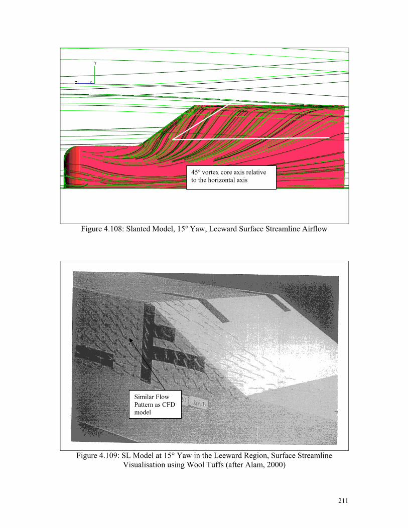
Figure 4.108: Slanted Model, 15° Yaw, Leeward Surface Streamline Airflow
45° vortex core axis relative to the horizontal axis
Similar Flow Pattern as CFD model
Figure 4.109: SL Model at 15° Yaw in the Leeward Region, Surface Streamline Visualisation using Wool Tuffs (after Alam, 2000)
211

Figure 4.110: Slanted Model, 15° Yaw, Windward Surface Streamline Airflow
Similar Flow Pattern as CFD model
Figure 4.111: SL Model at 15° Yaw in the Windward Region, Surface Streamline Visualisation using Wool Tuffs (after Alam, 2000)
212
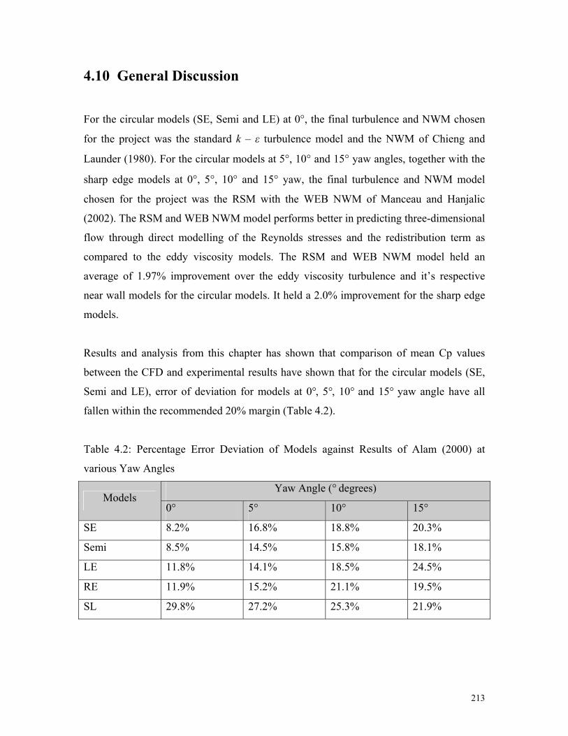
4.10 General Discussion
For the circular models (SE, Semi and LE) at 0°, the final turbulence and NWM chosen
for the project was the standard k – ε turbulence model and the NWM of Chieng and
Launder (1980). For the circular models at 5°, 10° and 15° yaw angles, together with the
sharp edge models at 0°, 5°, 10° and 15° yaw, the final turbulence and NWM model
chosen for the project was the RSM with the WEB NWM of Manceau and Hanjalic
(2002). The RSM and WEB NWM model performs better in predicting three-dimensional
flow through direct modelling of the Reynolds stresses and the redistribution term as
compared to the eddy viscosity models. The RSM and WEB NWM model held an
average of 1.97% improvement over the eddy viscosity turbulence and it’s respective
near wall models for the circular models. It held a 2.0% improvement for the sharp edge
models.
Results and analysis from this chapter has shown that comparison of mean Cp values
between the CFD and experimental results have shown that for the circular models (SE,
Semi and LE), error of deviation for models at 0°, 5°, 10° and 15° yaw angle have all
fallen within the recommended 20% margin (Table 4.2).
Table 4.2: Percentage Error Deviation of Models against Results of Alam (2000) at
various Yaw Angles
Yaw Angle (° degrees) Models
0° 5° 10° 15°
SE 8.2% 16.8% 18.8% 20.3%
Semi 8.5% 14.5% 15.8% 18.1%
LE 11.8% 14.1% 18.5% 24.5%
RE 11.9% 15.2% 21.1% 19.5%
SL 29.8% 27.2% 25.3% 21.9%
213

The best performing model was the SE model at 0° which yielded an under prediction of
8.2%. The worse performing model was the LE model at 15° yaw which yielded an under
prediction of 24.5%. For sharp edge models (RE and SL) error of deviation for models at
yaw angles of 0°, 5°, 10° and 15° yaw has also fallen within the recommended 20%
margin. The best performing model was the RE model at 0° which yielded an under
prediction of 11.9%. The worse performing model was the SL model at 0° yaw which
yielded an under prediction of 29.8%. Under predictions obtained through the turbulence
and near wall models occur within the vortex core area, in which the airflow were
experiencing vortex separation and reattachment. Comparison of airflow on the vehicle
surface between the CFD results and Alam (2000) showed that good correlation was
obtained. Comparisons were made for airflow streamline on the vehicle surface between
visuals obtained during the CFD post processing stage in the CFD model against wool
tuffs visualisation technique implemented by Alam (2000), which showed good
correlation with each other.
The size of the vortex measured for the various models at different yaw angles in the
leeward region of the flow suggest that with the circular models (SE, Semi and LE) and
the sharp edge models (RE and SL), the vortex size increases with yaw angles. This was
in agreement with Bearman et al. (1989) and Haruna et al. (1990). Refer Table 4.2.
Vortex measurement for the circular models at 40% scale shows that as the yaw angle
increases from 0° to 15° yaw, the vortex experiences a size increment of 225 mm in the
horizontal component and 328 mm in the vertical component. For the circular models, it
can be seen that the vortex is larger in the vertical component (430 mm at 15° yaw). The
vertical component also experiences a higher increase with an increase in yaw angles.
Table 4.3: Circular Models Vortex Size at 40% scale
Yaw Angles 0° 5° 10° 15°
Horizontal (mm) 115 150 214 340
Vertical (mm) 102 370 404 430
214

Vortex measurement for the RE model at 40% scale shows that as the yaw angle
increases from 0° to 15° yaw, the vortex experiences a size increment of 370 mm in the
horizontal component and 390 mm in the vertical component. For the RE model, it can be
seen that the vortex is larger in the vertical component (590 mm at 15° yaw). The vertical
component also experiences a higher increase with an increase in yaw angles. Refer
Table 4.3.
Table 4.4: RE Model Vortex Size at 40% scale
Yaw Angles 0° 5° 10° 15°
Horizontal (mm) 80 162 302 450
Vertical (mm) 200 487 554 590
Vortex measurement for the SL model at 40% scale shows that as the yaw angle
increases from 0° to 15° yaw, the vortex experiences a size increment of 330 mm in the
horizontal component and 60 mm in the vertical component. For the SL model, it can be
seen that the vortex is larger in the horizontal component (440 mm at 15° yaw). The
horizontal component also experiences a higher increase with an increase in yaw angles
(Table 4.4).
Table 4.5: SL Model Vortex Size at 40% scale
Yaw Angles 0° 5° 10° 15°
Horizontal (mm) 110 219 310 440
Vertical (mm) 360 330 320 380
The vortex core angle axis measured relative to the horizontal plane suggests that as the
yaw angle increases, the vortex core angle axis generally tend to increase. This finding
was consistent with the circular and SL model (Table 4.4). The RE model exhibits an
opposite trend to this finding (Table 4.3). Reason for this behaviour was due to the slant
angle of the windshield for the RE model. The windshield of the RE model is 90° to the
horizontal plane and not at 60° slant as per the other models. This difference in
windshield slant angle resulted in a decreasing vortex spread as the yaw angle increases.
215

It can be seen from Table 4.5 that the circular and the SL model experienced an increase
of 5° and 15° respectively when subjected to a 15° increase in yaw angle.
Table 4.6: Model vortex size increase with respect to the horizontal plane
Models 0° yaw 15° yaw
Circular 5° 10°
SL 30° 45°
RE 55° 38°
The results obtained from the CFD analysis shows that for both the circular and sharp
edge models, the source of vortex separation behind the A-pillar region originated from
the junction of the A-pillar base, the A-pillar apex and the front side window and roof
junction. This observation was in agreement with Hanaoka et al. (1993), Ahmed (1998)
and Zhu et al. (1993, 1994).
The flow separation behind the A-pillar region was a mixture of two dimensional and
three dimensional flows in which the determining factor of the flow mechanism lies in
the geometrical configuration of the source. Vortex originated from the A-pillar base
junction and the roof junction is two-dimensional free trailing helical vortices. Vortex
originated from the A-pillar edge/apex is either two-dimensional free trailing helical
vortices or three- dimensional helical vertically elongated cone shape vortices. This
observation is in agreement with Alam et al. (1998), Bearman et al. (1989), Haruna et al.
(1990) and Barnard (1996).
The mechanism of flow separation for both the circular and sharp edge models was due
to trailing edge separation in which the airflow that impinges on the windshield surface
started off as laminar flow. The laminar effect causes airflow to slide over each other due
to skin friction drag formed with the vehicle wall surface. This will cause the outer air
layer moving faster than the inner one which will slow down the flow, causing boundary
layer to gradually become thicker. As the formation of turbulent boundary layer
216

progressed, the flow becomes streamlined, following the contours of the vehicle body.
This was in agreement with Haruna et al. (1990) and Barnard (1996).
As the flow separates from the trailing edge, it was observed that region of adverse
pressure gradient was formed due to the rapid pressure change between layers of airflow.
This was in agreement with Roberson et al. (1997) and Hucho (1998). Viscous slipping
between adjacent layers of fluid molecules forces high air velocity flow on the outer layer
to glide pass the inner layer formation, causes airlfow to circulate, which forms the basis
of vortex formation, or ‘dead water’ zone, Hucho (1998). The area between region of
flow separation and reattachment is defined as ‘separation bubble’ region, Hucho (1998).
According to Watanabe et al. (1978) and Alam (2000) the vortex development forms
region of low relative pressure and that the core is located at the vortex core of the
separation. The shape of vortex formation varies between the circular and sharp edge
models.
For circular models, the shape of the vortices that takes place at 0° yaw took a physical
form of a two-dimensional quasi-elongated oval with a direction of flow moving
downstream to the flow. At 15° yaw, the shape of the vortices for the circular models
took an overall physical form of a three-dimensional mixture of a quasi circular and cone
shaped helical vortex, which was a chaotic combination of two-dimensional and three
dimensional vortices originating from the A-pillar base junction, apex and roof junction.
The axes of these vortices run essentially in the stream wise direction. The vortex is very
rich in kinetic energy and this containment in kinetic energy, which was determined by
the vehicle A- pillar angle inclination, Hucho (1998).
For the RE sharp edge model, shape of the localised vortices that takes place at 0° yaw
was a two-dimensional free trailing vortex originated from the base of the A-pillar
junction and a three-dimensional quasi circular cone shape helical vortex generated from
the A-pillar apex. The vortex generated from the roof junction formed a three-
dimensional circular shape vortex. All three form of vortices flowed in stream wise
direction, downstream to the flow. For the RE shape edge model at 15° yaw, the shape of
217

the vortex that takes place at the A-pillar base junction and A-pillar apex was similar to
that at 0° yaw. The vortices formed are very rich in kinetic energy, which propagated
downstream to the flow, continuing as free trailing vortices, Hucho (1998). The
perpendicular angle between the bonnet and windshield, also the windshield and the roof
causes the vortices to interfere with each other creating a chaotic turbulent structure.
Coupled with the yaw angle, the separation causes turbulent mixing, which translate to a
larger separation bubble and enhanced turbulent intensity. The physical shape of the
vortex for the RE model at yaw angles are similar to those of the circular models.
However, the turbulent intensity are higher in the RE model due to the influence of the
sharp A-pillar edge as compared to the streamlines curved A-pillar in the circular models.
For the SL sharp edge model, shape of the cortex that takes place at 0° yaw took a
physical form of a three-dimensional vertically elongated cone shape helical vortex
propagating downstream to the flow. At 0° yaw and 15° yaw, the shape of the vortex at
the A-pillar base junction, the A-pillar slant edge and the roof junction combine to form
the three dimensional conical helical vortex, making the turbulent intensity stronger as
the yaw angle increases. This was in agreement with Bearman et al. (1989). Changing
these parameters affects the intensity, size and shape of the vortex generated behind the
A-pillar region, Popat (1991). As the vortices propagates downstream to the flow,
turbulent mixing dissipates most of their kinetic energy making their development as
continuing free trailing vortices, often weak and even untraceable, Hucho (1998).
Turbulent intensity in the SL model is higher compared to the RE and circular models
respectively.
In the vortex structure, it was observed that the separated flow within the vortex region
exhibit rotational flow while the attached region remains irrotational, which was in
agreement with Haruna et al (1990). The small scale turbulent eddies are causing rapid
mixing. However, very close to the surface within a turbulent boundary layer flow, a thin
sub layer of laminar flow still exists. This result in a gradual increase in relative pressure
as the airflow moves downstream, which will have a direct impact on the process of
turbulent mixing. It will allow energy transfer to take place from the fast moving eddies
218

to the slower moving eddies in the turbulent boundary layer resulting in turbulent
boundary layer with low turbulent activity.
In a yaw angle scenario, it was observed that strong sideways or cross-stream
components on the surface of a vehicle complicate the formation and behaviour of the
boundary layer. Cross-stream components are more inclined to cause early transition of
the turbulent boundary layer. Cross-stream flows can also keep the boundary layer
attached by reducing high-pressure flow, making the pressure gradient less adverse. The
complex turbulence behaviour behind the A-pillar apex causes the vortex formed to
stretch and breakdown experiencing a decrease in magnitude intensity in the direction
normal to wall surface of the model and downstream to the flow. This is in line with the
findings of Laufer (1974) and Hussain (1983, 1986).
Overall, observation of various shapes of windshield radii and slant angle models
simulated in this project showed that the various geometrical configurations of the
windshield radii and slant angle governs the behaviour pattern of vortex generation
behind the A-pillar region. This was in agreement with Popat (1991), Hamel (1996) and
Hucho, (1998). The observations have showed that the vortex generated behind the A-
pillar region was lower in intensity and size in the circular models as compared to the
sharp edge models. The circular shape models windshield geometrical configuration and
slant angle created three different vortex formations, which determined the direction of
flow. The vortex generated from the various sources created a scenario whereby the
airflow path interferes with each other, creating a chaotic quasi-circular vortex structure
that prevents the formation of highly intense vortices behind the A-pillar region. This
scenario has the possibility to limit the generation of aerodynamic noise generated behind
the A-pillar region. The sharp edge models windshield geometrical configuration and
slant angle created a scenario whereby the airflow path from various directions converges
together effectively to form a highly intense three-dimensional helical cone shape vortex
all the way downstream to the flow. This produces high velocity region within the vortex,
which translate to a region of low negative pressure causing a vacuum like effect, which
was in agreement with Watanabe et al. (1978) and Alam (2000). When subjected to an
219

increased yaw angle, the vortex intensity, magnitude and size increases. This is due to the
formation of early boundary layer transition as a direct result from the change in airflow
angle of attack on the vehicle surface prior to separation. However again, this is
dependent on the geometrical configuration of the windshield radii and slant angle. The
turbulent intensity of the circular models at yaw angles is smaller compared to the sharp
edge models.
220

Chapter Five
COMPUTATIONAL AEROACOUSTICS (CAA)
SIMULATIONS
This chapter is divided into five sections. The first two section begins with the
introduction and methodology of the hybrid SWIFT CAA approach. The third section
describes the objectives and scope of this chapter. The fourth and fifth section will be the
presentation of results and discussion obtained through the SWIFT CAA simulation.
5.1 Introduction to the Hybrid SWIFT CAA Approach
As described previously in Chapter three, the CAA approach used for this research
project was based on the hybrid approach introduced by AVL/TNO through their CAA
SWIFT code, which was an extension to their CFD SWIFT code. In reiterating from
Chapter three, the main benefits and flexibility of using the hybrid CAA SWIFT
approach to determine aerodynamic acoustic propagation of a certain domain was to
bypass the necessity of:
• Generating computational domain with extremely large total grid count that
extends to the far field range in order to resolve the spatial and temporal scales.
• Conducting transient calculation using extremely small time scale that requires a
large amount of parallel computing resources.
• Modelling a large part of the upstream flow of the interested area in order to
generate an accurate noise prediction.
221
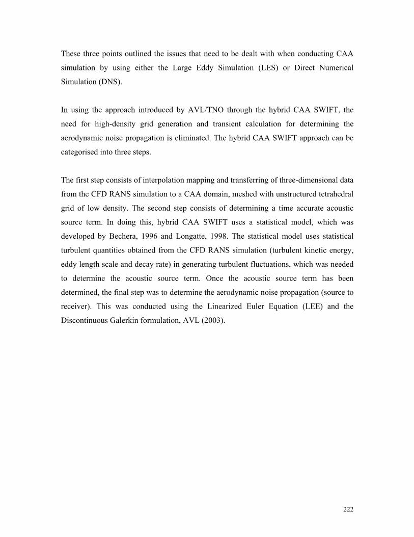
These three points outlined the issues that need to be dealt with when conducting CAA
simulation by using either the Large Eddy Simulation (LES) or Direct Numerical
Simulation (DNS).
In using the approach introduced by AVL/TNO through the hybrid CAA SWIFT, the
need for high-density grid generation and transient calculation for determining the
aerodynamic noise propagation is eliminated. The hybrid CAA SWIFT approach can be
categorised into three steps.
The first step consists of interpolation mapping and transferring of three-dimensional data
from the CFD RANS simulation to a CAA domain, meshed with unstructured tetrahedral
grid of low density. The second step consists of determining a time accurate acoustic
source term. In doing this, hybrid CAA SWIFT uses a statistical model, which was
developed by Bechera, 1996 and Longatte, 1998. The statistical model uses statistical
turbulent quantities obtained from the CFD RANS simulation (turbulent kinetic energy,
eddy length scale and decay rate) in generating turbulent fluctuations, which was needed
to determine the acoustic source term. Once the acoustic source term has been
determined, the final step was to determine the aerodynamic noise propagation (source to
receiver). This was conducted using the Linearized Euler Equation (LEE) and the
Discontinuous Galerkin formulation, AVL (2003).
222

5.2 Methodology of the Hybrid SWIFT CAA Approach
The first step in the hybrid SWIFT CAA approach was to use the CAA Mapper to
interpolate and map three-dimensional statistical turbulent quantities from the CFD
domain to the CAA domain. In order to initialise and employ the CAA Mapper, the CAA
domain however, must first be created.
The CAA domain creation involves a five-step process. The first step in creating the
CAA domain was to select and extract an area of interest from within the CFD domain.
In the context of this research project, the area of interest consists of the surrounding
section containing the A-pillar. The second step involves in creating a triangulate surface
area from the selected CFD domain extraction using the Triangulation function in the
AVL SWIFT Surface Tool section. The third step was to mesh the triangulate surface
area with unstructured tetrahedral grids by using the FAME-TET function in the AVL
SWIFT Mesh Tool section. The fourth step involves inspecting the newly created
unstructured tetrahedral mesh to ensure that it was void of negative volume and negative
normal. In addition, each grid cell in the CAA domain must also adhere to an aspect ratio
of smaller than 3.3 in order to maintain optimum accuracy. Should problems occur due to
the presence of negative volume or normals or due to high value of aspect ratio, changes
can be made through altering the values within the FAME-TET function. The final step
in creating the CAA domain was to assign boundary conditions to each external surface
of the volume. External surface boundaries can be assigned with either a reflecting (wall
of the CAA domain) or non-reflecting (inlet and outlet of the CAA domain) boundary
condition. The name assigned to the reflecting boundary condition must start with the
letter “W” and the name assigned to the non-reflecting boundary condition must start
with the letter “N”.
However, simplified vehicle model used in this project especially with rounded
windshield configuration and with yawed orientation, creating unstructured tetrahedral
grids for the CAA domain was proved to be a difficult exercise since the models
experienced a resultant aspect ratio of larger than 3.3. To overcome this problem, the
223

unstructured tetrahedral was created instead using GAMBIT, from FLUENT. In
GAMBIT, the geometry of the CAA domain of interest was first created and then meshed
with unstructured tetrahedral grids. The file from GAMBIT was then exported to
FLUENT before being saved in a Nastran .BDF file format. The Nastran file was then
finally imported using AVL SWIFT and saved as an AVL SWIFT (.FLM) volume file.
For the unstructured tetrahedral grids created using the AVL SWIFT functions, each grid
size was of 50 mm interval. For the tetrahedral mesh created from GAMBIT, each grid
size is of 100 mm interval. Examples of unstructured tetrahedral CAA domain created
from AVL SWIFT and GAMBIT can be seen in Figure 5.1.
Figure 5.1 Unstructured Tetrahedral CAA Domain of Various Simplified Vehicle Model
Created from AVL SWIFT and GAMBIT
224

The final mesh count from the unstructured tetrahedral grids generated for the CAA
domain varies from one simplified vehicle model to the other. Factors that determined the
final mesh generation were the yaw angle orientation of the CAA domain and also the
different approach in softwares selection used in creating the CAA domain. Unstructured
tetrahedral mesh generated using AVL SWIFT varied in between 14,000 to 35,000 grid
cells. Mesh generated using GAMBIT varies in between 5,000 to 17,000 grid cells.
Once the CAA domain (unstructured tetrahedral mesh) has been constructed, the CAA
Mapper was then used to map the three-dimensional statistical turbulence quantities from
the CFD simulation through the process of interpolation. Dividing the CAA domain into
several rectangular partitions or bins accelerates the mapping and interpolation process.
The user has to specify the amount of bin in the X, Y and Z direction with a maximum
total allowable of 150 bins (X*Y*Z). In this research project, the amount of allocated bins
was set as default. In addition, the amount of CFD nodes that are being interpolated in
each bin must be sufficiently high to ensure an accurate mapping. The user was allowed
to set an interpolation value of between 5 to 20 CFD nodes per CAA node to be mapped
in each bin. In this research project, the node interpolation value was set as 10, which was
the default value. Once the mapping and interpolation process was completed, the CAA
Mapper was then able to establish an initial time step to be used in the CAA solver. The
initial time step estimate was based on the velocity used in the calculation together with
the grid size and the Courant number. It was therefore important to establish the most
efficient mesh count in order to obtain a reasonable time step interval for the final
simulation in the CAA solver.
As with the final resulting grid size of the unstructured grids, the final resulting time
interval for the CAA domain varied from one simplified vehicle model to the other.
Unstructured tetrahedral grids generated using AVL SWIFT varied between 4.0 to 6.0 μ-
seconds and took between 160,000 to 200,000 time steps to complete an overall 1.0-
second time interval propagation. Grids generated using GAMBIT on the other hand
varied between 3.0 to 16.0 μ-seconds and will take between 60,000 to 270,000 time steps
to complete an overall 1.0-second time interval propagation. The time interval
225
propagation used for this project was for only 1.0 second as oppose to 10.0 seconds by
Alam (2000). Further explanation on this selection will be provided in the following
section.
The second and final step in the hybrid SWIFT CAA approach was to use the CAA
solver to determine the time accurate acoustic source terms and to finally determine the
aerodynamic noise propagation by using the Linearized Euler Equation (LEE) and the
Discontinuous Galerkin formulation.
In order to first determine the time accurate acoustic source terms, the workings of the
fundamental equations must first be understood. Starting from the derivation of
conserved equations of mass, momentum and energy (equations 3.161 to 3.164), it was
established that five unknowns exists [density, velocity (three components) and pressure].
The five unknowns are then separated into its mean, acoustic and turbulent component as
per equations 3.165 to 3.167. By using LEE, the separated components of density,
pressure and velocity was then substituted into the conserved equations of mass,
momentum and energy. From there, further derivation took place which in the end
produced three acoustic source terms (equations 3.177 to 3.179).
In order to determine the acoustic source term, the turbulent velocity must first (which
exists as an unknown) need to be ascertained. This was done through the statistical model
developed by Bechera (1996) and Longatte (1998). The statistical model used
information from the statistical turbulent quantities obtained from the CFD RANS
simulation (turbulent kinetic energy, eddy length scale and decay rate) to generate
turbulent fluctuations, which were needed to determine the acoustic source term. The
acoustic source term was generated through the Unstructured Kinematic Source
Generator (UKSG) in the CAA solver. According to AVL (2003), turbulent velocities
were determined through the use of inverse Fourier transform. The inverse Fourier
transform distributes the turbulent velocities as superposition of modes. Each inverse
Fourier transform mode was assigned with a mode amplitude, random frequency and
random phase. The mode amplitude was determined through the use of a modified Von
226
Karman energy spectrum (which assumes to be incompressible and isotropic) in which
rely on the turbulent kinetic energy and dissipation length scale results from the CFD
RANS simulation. The inverse Fourier transform formulation was then completed by
adding a temporal component to the inverse Fourier transform, in which the spatial and
temporal coupling between the turbulence and the mean flow was conducted through the
introduction of a moving axis spectrum. Finally, the acoustic source term was then
obtained through the differentiation of the Lighthill Stress Tensor components. These
source terms are calculated for each element in the CAA domain.
The final step in the CAA solver is to determine aerodynamic acoustic propagation
through solving the LEE (equations 3.189 to 3.195). This was done from within the CAA
solver by the DIGS3D subroutine. According to AVL (2003), this calculation was
conducted in the time domain by using a Quadrature Free Discontinuous Galerkin Spatial
discretization approach. In this approach, the revised source term obtained progressively
at each time interval from the UKSG subroutine was interpolated to the CAA solver. A
new time step interval was then obtained through the use of a fourth-order Runge-Kutta
algorithm.
In setting up the CAA solver to simulate for the aerodynamic acoustic propagation, most
of the input parameter in the Solver Steering File (Case File) was set as default. The input
parameters that were revised were the Turbulence Realization Sampling Frequency and
the Input Coordinates for Microphone Location. The values assigned for the Turbulence
Realization Sampling Frequency was 40,000 Hz, which was the maximum allowed. This
was close to the value of 48,000 Hz, which was used by Alam (2000). The input
coordinates for the microphone locations was assigned for all 16 points for the bottom
and top row along the allocated area behind the A-pillar region. For yaw cases,
coordinates were assigned to A-pillars in the windward and leeward region.
Once the input in the Solver Steering File has been finalised, the CAA solver will process
the calculation for the aerodynamic acoustic propagation. The duration of each simulation
varies with each simplified vehicle model. Depending on the size of the CAA domain
227
(total mesh) and time step interval, the simulation took between one to four days to
finish. This is also dependent on the computational processing capabilities. Calculation of
the CAA solver for this project was done using only a single processor in the Swinburne
University Super Computer cluster. Once the CAA solver has finished processing, the
data was analysed using post-processing features available in AVL SWIFT. Post
processing features such as Power Spectral Density (PSD) analysis were obtained by
providing input such as the number of Fourier Fast Transform (FFT) blocks, Number of
FFT overlap points and viewing Window for each Fourier block. For this research
project, the inputs were obtained from Alam (2000) which were as follows:
• Number of FFT blocks – 4096
• Number of FFT overlap points – 50%
• Viewing Window for each block – Hanning
5.3 Objectives & Scope of using Hybrid SWIFT CAA
Approach: Application to this Research Project
There are two main objectives in the context of applying the CAA approach to this
research project. The first main objective is to validate the Hybrid SWIFT CAA approach
in modelling aeroacoustics behaviour of airflow around the vehicle A-pillar region
numerically through the application of the CFD modelling results obtained. The choice of
using the Hybrid SWIFT CAA approach was based on the simple approach that it
promised, which was discussed earlier in section 5.1. Validation of the Hybrid SWIFT
CAA approach in this chapter will be carried out through comparison of results with
results obtained experimentally by Alam (2000).
The second main objective is to extend the knowledge on the study of aeroacoustics
behaviour of airflow around the A-pillar region, possibly linking it to the aerodynamics
behaviour, which was presented and discussed in Chapter 4. From the knowledge
228

obtained while researching for this project through reviews of literatures (Chapter 2), the
following questions were raised and will be addressed to in this chapter.
In the context of transient flow condition of airflow around the A-pillar region,
when does each simplified vehicle model approach steady state condition? Will
different yaw orientation have any effect on this?
What are the aero acoustics behaviour and distribution patterns that can be
established in terms of OASPL magnitude at steady and transient condition of
different simplified vehicle model at different yaw orientation?
How is the aero acoustics behaviour behind the A-pillar region linked with the
aerodynamics behaviour at different simplified vehicle model at different yaw
orientation?
Therefore, the objectives along with the scope of this chapter will be as follows:
5.3.1 Objectives of Chapter 5
1. To validate the Hybrid SWIFT CAA modelling of the aero acoustics of airflow
behaviour surrounding the vehicle A-pillar region with the existing experimental
results of Alam (2000).
2. To determine the temporal transition between transient and steady state flow
condition of airflow around the A-pillar region at different yaw orientation.
3. To determine the behaviour and distribution mode of OASPL magnitude at steady
state and transient condition surrounding the A-pillar region within the vicinity of
the CAA domain at different yaw orientation.
229
4. To link the aero acoustics and aerodynamic behaviour behind the A-pillar region
for at different yaw orientation.
5.3.2 Scope of Chapter 5
1. All simplified models (RE (Rectangular), SL (Slanted Edge), SE (Small
Ellipsoidal), Semi (Semi Circular), and LE (Large Ellipsoidal)).
2. Simplified model yaw orientation of 0° and 15°.
3. Wind tunnel inlet velocity of 60, 100 and 140 km/h. For objectives number two to
five, wind tunnel inlet velocity of only 140 km/h will be used.
4. Time interval of 1.0 second.
230
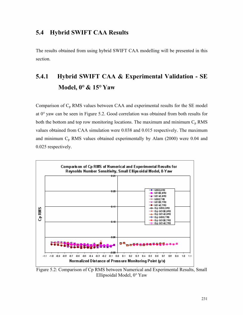
5.4 Hybrid SWIFT CAA Results
The results obtained from using hybrid SWIFT CAA modelling will be presented in this
section.
5.4.1 Hybrid SWIFT CAA & Experimental Validation - SE
Model, 0° & 15° Yaw
Comparison of Cp RMS values between CAA and experimental results for the SE model
at 0° yaw can be seen in Figure 5.2. Good correlation was obtained from both results for
both the bottom and top row monitoring locations. The maximum and minimum Cp RMS
values obtained from CAA simulation were 0.038 and 0.015 respectively. The maximum
and minimum Cp RMS values obtained experimentally by Alam (2000) were 0.04 and
0.025 respectively.
Figure 5.2: Comparison of Cp RMS between Numerical and Experimental Results, Small
Ellipsoidal Model, 0° Yaw
231

Comparison of Cp RMS values obtained for the SE model at 15° yaw between the CAA
simulation and experimental results can be seen on Figure 5.3. It can be seen from Figure
5.3 that correlation between experimental and CAA simulation results were similar in the
windward region for both the bottom and top row monitoring locations. However, small
discrepancies exist in the leeward region, particularly in the halfway point of the bottom
row monitoring locations and towards the end of the top row monitoring locations
respectively, Murad (2006). The maximum Cp RMS obtained for the SE Model at 15°
yaw at the leeward and windward region from the CAA simulation was 0.048 and 0.039
respectively. The minimum Cp RMS value that was obtained at the leeward and
windward region was 0.027 and 0.022 respectively. The maximum Cp RMS value in the
leeward and windward region obtained experimentally by Alam (2000) was 0.13 and
0.045. The minimum Cp RMS value in the leeward and windward region obtained
experimentally by Alam (2000) was 0.04 and 0.035 respectively.
Figure 5.3: Comparison of Cp RMS between Numerical and Experimental Results, Small
Ellipsoidal Model, -15° Yaw
The comparison of PSD distribution between CAA simulation and experimental results
obtained for SE model of 0°, -15° and +15° yaw angle at 100 km/h can be seen in Figure
5.4. From the CAA simulation results in Figure 5.4, it can be seen that the highest
prediction of PSD distribution occurred at -15° yaw, followed by +15° and 0° yaw
232

respectively. The peak OASPL value obtained from the CAA simulation results at -15°
yaw was measured at 99-dB followed by +15° yaw measured at 98-dB. Finally, peak
OASPL value obtained from CAA results at 0° yaw was measured at 100-dB. Results
obtained experimentally from Alam (2000) yielded peak OASPL value at -15° yaw
measured around 113-dB, followed by a measurement of 101-dB at 0° yaw (Figure 5.7).
Finally a measurement of 95-dB was obtained at +15° yaw orientation. Difference
between peak OASPL values between CAA and experimental results yielded lowest
discrepancies at 0° yaw, followed by +15° yaw and -15° yaw, measuring 1.0-dB, 3.0-dB
and 14.0-dB respectively, Murad (2006).
Cross Over at 3-kHz
Cross Over at 500-Hz Cross Over at
6-kHz
Figure 5.4: Power Spectral Density (PSD) Distribution of Maximum RMS Pressure, Small Ellipsoidal Model, 0°, -15° and +15° Yaw, 100 km/h, 0 to 8-kHz Frequency Region
233
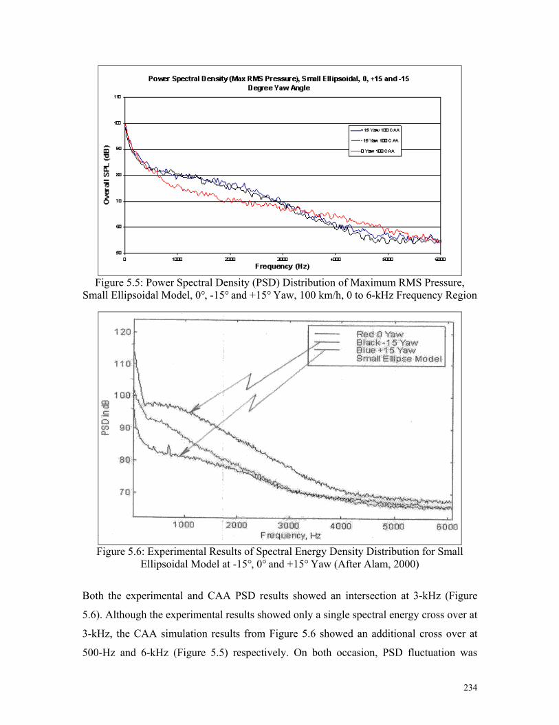
Figure 5.5: Power Spectral Density (PSD) Distribution of Maximum RMS Pressure,
Small Ellipsoidal Model, 0°, -15° and +15° Yaw, 100 km/h, 0 to 6-kHz Frequency Region
Figure 5.6: Experimental Results of Spectral Energy Density Distribution for Small
Ellipsoidal Model at -15°, 0° and +15° Yaw (After Alam, 2000)
Both the experimental and CAA PSD results showed an intersection at 3-kHz (Figure
5.6). Although the experimental results showed only a single spectral energy cross over at
3-kHz, the CAA simulation results from Figure 5.6 showed an additional cross over at
500-Hz and 6-kHz (Figure 5.5) respectively. On both occasion, PSD fluctuation was
234

observed originating from the model at 0° yaw angle. The overall PSD distribution
discrepancy below 3-kHz, was measured at 1.0-dB, 5.5-dB and 12.5-dB, corresponding
to yaw angles at +15°, 0° and -15° respectively. The overall PSD discrepancies obtained
above 3-kHz was 9.0-dB, 9.0-dB and 14.0-dB, corresponding to yaw angles at +15°, 0°
and -15° respectively. In summary, the overall PSD distribution for SE model showed
best correlation at yaw angle of +15°, followed by yaw angles of 0°-yaw and -15°-yaw,
with discrepancies (combining discrepancies for below and above 3-kHz) measured at
5.0-dB, 7.3-dB and 13.3-dB respectively. Discrepancies in the CAA results is caused by
the discrepancies obtained in the earlier CFD models (discussed in Chapter 4) and also
due to numerical discrepancies caused by the acoustical model used in software to
determine the acoustical propagation estimation.
5.4.2 Hybrid SWIFT CAA & Experimental Validation -
Semi Model, 0° & 15° Yaw
Comparison between experimental and CAA results of Cp RMS values for the Semi
model at 0° yaw can be seen in Figure 5.7. Good correlation was obtained from both
results for both the bottom and top row monitoring locations. The maximum and
minimum Cp RMS values obtained from the CAA simulation were 0.067 and 0.044
respectively. The maximum and minimum Cp RMS values obtained experimentally by
Alam (2000) were 0.05 and 0.025 respectively. This discrepancy in results is small and
acceptable due to the constant fluctuating of acoustical pressure prior conversion to Cp
RMS values.
The Cp RMS results for the Semi model at 15° yaw obtained from the CAA simulation
can be seen on Figure 5.8. It can be seen from Figure 5.8 that correlation between
experimental and CAA simulation results in the leeward and windward region yielded
small discrepancies, particularly towards the rear portion of the bottom and top row
monitoring points.
235
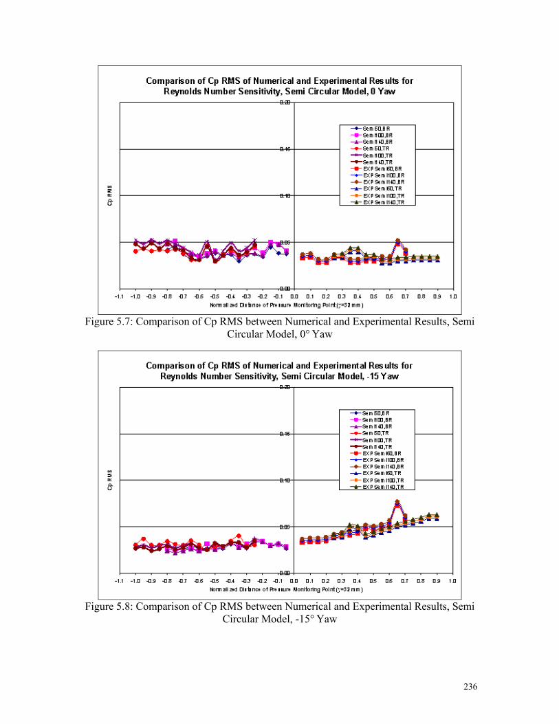
Figure 5.7: Comparison of Cp RMS between Numerical and Experimental Results, Semi
Circular Model, 0° Yaw
Figure 5.8: Comparison of Cp RMS between Numerical and Experimental Results, Semi
Circular Model, -15° Yaw
236
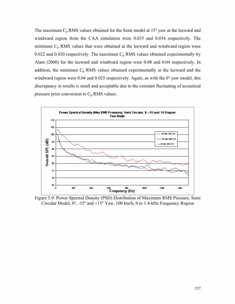
The maximum Cp RMS values obtained for the Semi model at 15° yaw at the leeward and
windward region from the CAA simulation were 0.035 and 0.034 respectively. The
minimum Cp RMS values that were obtained at the leeward and windward region were
0.022 and 0.020 respectively. The maximum Cp RMS values obtained experimentally by
Alam (2000) for the leeward and windward region were 0.08 and 0.04 respectively. In
addition, the minimum Cp RMS values obtained experimentally at the leeward and the
windward region were 0.04 and 0.025 respectively. Again, as with the 0° yaw model, this
discrepancy in results is small and acceptable due to the constant fluctuating of acoustical
pressure prior conversion to Cp RMS values.
Figure 5.9: Power Spectral Density (PSD) Distribution of Maximum RMS Pressure, Semi
Circular Model, 0°, -15° and +15° Yaw, 100 km/h, 0 to 1.4-kHz Frequency Region
237

Figure 5.10: Experimental Results of Spectral Energy Density Distribution for Semi
Circular Model at -15°, 0° and +15° Yaw (After Alam, 2000)
The comparison of PSD distribution between CAA simulation and experimental results
obtained for Semi model of 0°, -15° and +15° yaw angle at 100 km/h can be seen in
Figure 5.9. From the CAA simulation results in Figure 5.9, it can be seen that throughout
the PSD distribution, the model at 0° yaw experienced the highest prediction of PSD
distribution. These were followed by +15° and -15° yaw respectively. The experimental
results produced the highest PSD distribution at the -15° yaw model, followed by the 0°
yaw and +15° yaw respectively (Figure 5.10).
From the CAA simulation results, the peak OASPL value obtained at 0° yaw was
measured at 103-dB followed by -15° yaw measured at 102-dB. Finally, maximum
OASPL value obtained at +15° yaw was measured at 98-dB. Results obtained
experimentally from Alam (2000) yielded peak OASPL value at -15° yaw measured
around 120-dB, followed by a measurement of 117-dB at 0° and +15° yaw respectively.
Comparison of peak PSD values between CAA and experimental results yielded lowest
discrepancy at 0° yaw, followed by -15° and +15° yaw, measuring 14.0-dB, 18.0-dB and
19-dB respectively, Murad (2006).
238

Overall, the PSD distribution prediction was at its most consistent for model at 0°,
followed by models at +15° and -15° yaw respectively. These corresponds to mean
average discrepancies (combining discrepancies at peak and minimum OASPL) of 7-dB,
12-dB and 15-dB in magnitude for yaw angle of 0°, +15° and -15° yaw respectively.
5.4.3 Hybrid SWIFT CAA & Experimental Validation - LE
Model, 0° & 15° Yaw
Comparison between experimental and CAA results of Cp RMS values for the LE model
at 0° yaw can be seen in Figure 5.11. Good correlation was obtained from both results for
both the bottom and top row monitoring locations. However, comparison of results
showed small discrepancy at 0º yaw and 100 km/h, caused probably by discretization
error. The maximum and minimum Cp RMS values obtained from the CAA simulation
were 0.063 and 0.021 respectively. The maximum and minimum Cp RMS values
obtained experimentally by Alam (2000) were 0.040 and 0.08 respectively.
The Cp RMS results for the LE model at 15° yaw obtained from the CAA simulation can
be seen on Figure 5.12. It can be seen from Figure 5.12 that correlation between
experimental and CAA simulation results were similar in the leeward and windward
region for both the bottom and top row monitoring locations. However, small
discrepancies exist around the frontal portion of the bottom and top monitoring locations
of the windward region. The maximum Cp RMS values obtained for the LE model at 15°
yaw at the leeward and windward region from the CAA simulation were 0.044 and 0.033
respectively. The minimum Cp RMS values that were obtained at the leeward and
windward region were 0.026 and 0.045 respectively. The maximum Cp RMS values
obtained experimentally by Alam (2000) for the leeward and windward region were
0.046 and 0.045 respectively. The minimum Cp RMS values obtained experimentally at
the leeward and the windward region was 0.121 and 0.067 respectively.
239

Figure 5.11: Comparison of Cp RMS between Numerical and Experimental Results,
Large Ellipsoidal Model, 0° Yaw
Figure 5.12: Comparison of Cp RMS between Numerical and Experimental Results,
Large Ellipsoidal Model, -15° Yaw
240
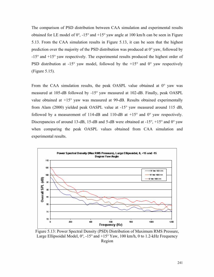
The comparison of PSD distribution between CAA simulation and experimental results
obtained for LE model of 0°, -15° and +15° yaw angle at 100 km/h can be seen in Figure
5.13. From the CAA simulation results in Figure 5.13, it can be seen that the highest
prediction over the majority of the PSD distribution was produced at 0° yaw, followed by
-15° and +15° yaw respectively. The experimental results produced the highest order of
PSD distribution at -15° yaw model, followed by the +15° and 0° yaw respectively
(Figure 5.15).
From the CAA simulation results, the peak OASPL value obtained at 0° yaw was
measured at 105-dB followed by -15° yaw measured at 102-dB. Finally, peak OASPL
value obtained at +15° yaw was measured at 99-dB. Results obtained experimentally
from Alam (2000) yielded peak OASPL value at -15° yaw measured around 115 dB,
followed by a measurement of 114-dB and 110-dB at +15° and 0° yaw respectively.
Discrepancies of around 13-dB, 15-dB and 5-dB were obtained at -15°, +15° and 0° yaw
when comparing the peak OASPL values obtained from CAA simulation and
experimental results.
Figure 5.13: Power Spectral Density (PSD) Distribution of Maximum RMS Pressure, Large Ellipsoidal Model, 0°, -15° and +15° Yaw, 100 km/h, 0 to 1.2-kHz Frequency
Region
241

Cross Over at 2.2-kHz Cross Over at
5.2-kHz
Figure 5.14: Power Spectral Density (PSD) Distribution of Maximum RMS Pressure, Large Ellipsoidal Model, 0°, -15° and +15° Yaw, 100 km/h, 0 to 8.0-kHz Frequency
Region
Figure 5.15: Experimental Results of Spectral Energy Density Distribution for Large
Ellipsoidal Model at -15°, 0° and +15° Yaw (After Alam, 2000)
242
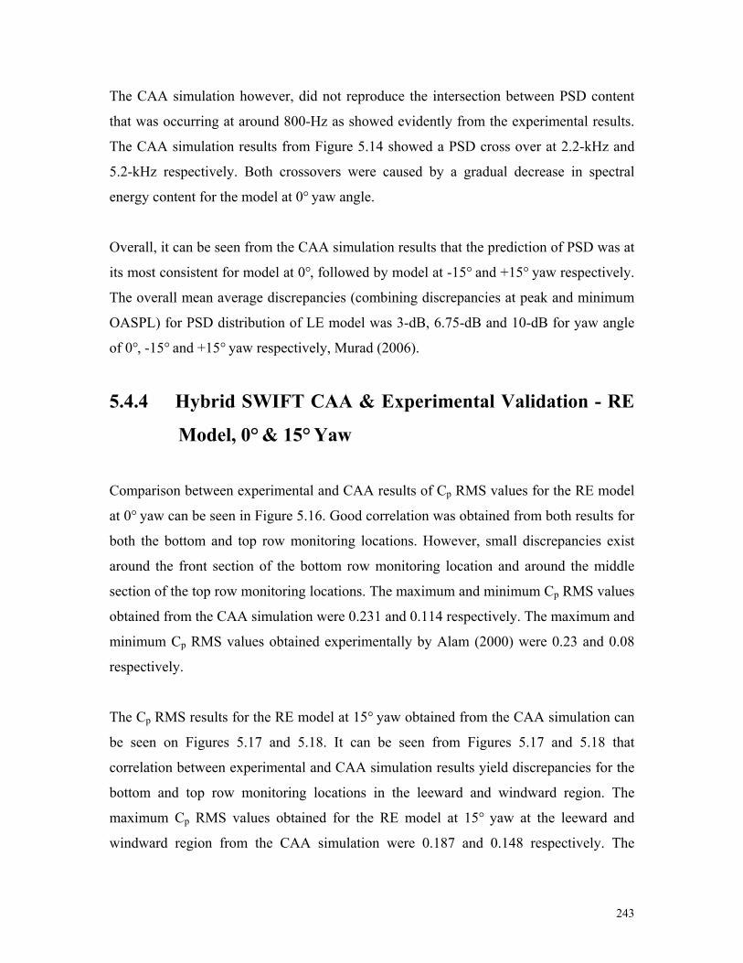
The CAA simulation however, did not reproduce the intersection between PSD content
that was occurring at around 800-Hz as showed evidently from the experimental results.
The CAA simulation results from Figure 5.14 showed a PSD cross over at 2.2-kHz and
5.2-kHz respectively. Both crossovers were caused by a gradual decrease in spectral
energy content for the model at 0° yaw angle.
Overall, it can be seen from the CAA simulation results that the prediction of PSD was at
its most consistent for model at 0°, followed by model at -15° and +15° yaw respectively.
The overall mean average discrepancies (combining discrepancies at peak and minimum
OASPL) for PSD distribution of LE model was 3-dB, 6.75-dB and 10-dB for yaw angle
of 0°, -15° and +15° yaw respectively, Murad (2006).
5.4.4 Hybrid SWIFT CAA & Experimental Validation - RE
Model, 0° & 15° Yaw
Comparison between experimental and CAA results of Cp RMS values for the RE model
at 0° yaw can be seen in Figure 5.16. Good correlation was obtained from both results for
both the bottom and top row monitoring locations. However, small discrepancies exist
around the front section of the bottom row monitoring location and around the middle
section of the top row monitoring locations. The maximum and minimum Cp RMS values
obtained from the CAA simulation were 0.231 and 0.114 respectively. The maximum and
minimum Cp RMS values obtained experimentally by Alam (2000) were 0.23 and 0.08
respectively.
The Cp RMS results for the RE model at 15° yaw obtained from the CAA simulation can
be seen on Figures 5.17 and 5.18. It can be seen from Figures 5.17 and 5.18 that
correlation between experimental and CAA simulation results yield discrepancies for the
bottom and top row monitoring locations in the leeward and windward region. The
maximum Cp RMS values obtained for the RE model at 15° yaw at the leeward and
windward region from the CAA simulation were 0.187 and 0.148 respectively. The
243

minimum Cp RMS values that were obtained at the leeward and windward region were
0.098 and 0.067 respectively. The maximum Cp RMS values obtained experimentally by
Alam (2000) for the leeward and windward region were 0.33 and 0.4 respectively. The
minimum Cp RMS values obtained experimentally at the leeward and the windward
region was 0.07 and 0.04 respectively.
Figure 5.16: Comparison of Cp RMS between Numerical and Experimental Results,
Rectangular Edge Model, 0° Yaw
244

Figure 5.17: Comparison of Cp RMS between Numerical and Experimental Results,
Rectangular Edge Model, -15° Yaw
Figure 5.18: Comparison of Cp RMS between Numerical and Experimental Results,
Rectangular Edge Model, +15° Yaw
245

The comparison of PSD distribution between CAA simulation and experimental results
rom the CAA simulation results, the peak OASPL value obtained at 0° yaw was
obtained for RE model of 0°, -15° and +15° yaw angle at 100 km/h can be seen in Figure
5.19. From the CAA simulation results in Figure 5.19, it can be seen that the prediction of
highest order of PSD distribution occurred at 0° yaw, followed by -15° and +15° yaw
respectively. It can be seen from Figure 5.19 that the CAA results produced a PSD cross
over at 4000 Hz. The cross over was caused by a gradual decrease in spectral energy
content for the model at -15° yaw angle.
F
measured at 117-dB followed by -15° yaw measured at 116-dB. Finally, peak OASPL
value obtained at +15° yaw was measured at 109-dB. Results obtained experimentally
from Alam (2000) yielded a peak OASPL value at -15° yaw measured around 126.5-dB,
followed by peak values of 128-dB and 124-dB at +15° and 0° yaw respectively.
Discrepancies of 10.5-dB, 19-dB and 7-dB were obtained at -15°, +15° and 0° yaw when
comparing the peak OASPL values obtained between CAA and experimental results.
Cross Over at 4.0-kHz
Figure 5.19: Power Spectral Density (PSD) Distribution of Maximum RMS Pressure, Rectangular Edge Model, 0°, -15° and +15° Yaw, 100 km/h, 0 to 8.0-kHz Frequency
Region
246

Figure 5.20: Experimental Results of Spectral Energy Density Distribution for
Rectangular Edge Model at -15°, 0° and +15° Yaw (After Alam, 2000)
Overall, the CAA simulation results prediction of PSD distribution was most consistent
for model at 0°, followed by model at -15° and +15° yaw respectively. The overall mean
average discrepancies (combining discrepancies at peak and minimum OASPL) of PSD
distribution for RE model was 7-dB, 8.3-dB and 13-dB for yaw angle of 0°, -15° and +15°
yaw respectively.
5.4.5 Hybrid SWIFT CAA & Experimental Validation - SL
Model, 0° & 15° Yaw
Comparison between experimental and CAA results of Cp RMS values for the SL model
at 0° yaw can be seen in Figure 5.21. It can be seen from Figure 5.21 that correlation
between experimental and CAA simulation results yield discrepancies at the bottom and
top row monitoring locations. This was particularly evident in both frontal section of the
bottom and top row monitoring locations. The maximum and minimum Cp RMS values
obtained from the CAA simulation were 0.21 and 0.07 respectively. The maximum and
247

minimum Cp RMS values obtained experimentally by Alam (2000) were 0.28 and 0.03
respectively. However, similar experimental testing using SL model, which was
conducted by Popat (1991), yielded Cp RMS values of a maximum and minimum value
of 0.21 and a 0.06 respectively.
The Cp RMS results for the SL model at 15° yaw obtained from the CAA simulation can
be seen on Figure 5.22 and 5.23 respectively. It can be seen from Figure 5.22 and 5.23
that comparison between experimental and CAA simulation results yielded discrepancies
for the bottom and top row monitoring locations in the leeward and windward region.
This was particularly evident in the middle section of the bottom and top row monitoring
locations in the leeward region. In the windward region, discrepancies were observed in
the frontal section of the bottom and top row monitoring locations. The maximum Cp
RMS values obtained for the Slanted Edge model at 15° yaw at the leeward and
windward region from the CAA simulation were 0.16 and 0.1 respectively. The minimum
Cp RMS values that were obtained at the leeward and windward region were 0.06 and
0.049 respectively. The maximum Cp RMS values obtained experimentally by Alam
(2000) for the leeward and windward region were 0.41 and 0.11 respectively. The
minimum Cp RMS values obtained experimentally at the leeward and the windward
region was 0.08 and 0.02 respectively.
248

Figure 5.21: Comparison of Cp RMS between Numerical and Experimental Results,
Slanted Edge Model, 0° Yaw
Figure 5.22: Comparison of Cp RMS between Numerical and Experimental Results,
Slanted Edge Model, -15° Yaw
249

Figure 5.23: Comparison of Cp RMS between Numerical and Experimental Results,
Slanted Edge Model, +15° Yaw
The comparison of PSD distribution between CAA simulation and experimental results
obtained for SL model of 0°, -15° and +15° yaw angle at 100 km/h can be seen in Figures
5.24 and 5.25. From the CAA simulation results, the peak OASPL value obtained at 0°
yaw was measured at 112.5-dB followed by +15° yaw measured at 109-dB. Finally, peak
OASPL value obtained at -15° yaw was measured at 102.5-dB. Results obtained
experimentally from Alam (2000) yielded a peak OASPL value at -15° yaw measured
around 129-dB, followed by a measurement of 116-db and 123-dB at +15° and 0° yaw
respectively. Discrepancies of 26.5-dB, 7-dB and 10.5-dB were obtained at -15°, +15°
and 0° yaw when comparing the peak OASPL values obtained from CAA simulation and
experimental results.
The overall PSD distribution prediction from the CAA simulation results was at its most
consistent at 0°, followed by model at -15° and +15° yaw respectively. This corresponds
to the total mean average discrepancies (combining discrepancies at peak and minimum
OASPL) of 15.3-dB, 17-dB and 5.3-dB for SL model at yaw angle of 0°, -15° and +15°
yaw respectively.
250

Cross Over at 230-Hz
Cross Over at 4.5-kHz
Figure 5.24: Power Spectral Density (PSD) Distribution of Maximum RMS Pressure, Slanted Edge Model, 0°, -15° and +15° Yaw, 100 km/h, 0 to 8.0-kHz Frequency Region
Cross Over at 230-Hz
Cross Over at 4.5-kHz
Figure 5.25: Experimental Results of Spectral Energy Density Distribution for Slanted Edge Model at -15°, 0° and +15° Yaw (After Alam, 2000)
251

5.4.6 Aeroacoustics Behaviour during Transient Condition -
SE Model, 0° & 15° Yaw
Figure 5.26 and 5.27 presents the mean and RMS transient pressure distribution for the
SE model at 0° and 15° yaw over a one second time interval march. The pressure
monitoring point was plotted at the front section of the bottom row monitoring location of
the A-pillar region. The transient progression of the model was divided into three stages,
namely the random fluctuating stage, the transition stage and the steady state stage. At the
end of the random fluctuating and transition stage, the time mean average at 60, 100 and
140 km/h were taken to determine the time taken for each stage to end. At 0° yaw, the
mean average of the random fluctuating stage ended at 0.08 second while the mean
average of the transition stage ended at 0.19 second. Therefore, the random fluctuating
stage was between 0 and 0.08 second, while the transition stage was between 0.08 and
0.19 second. The flow finally stabilised into a steady state condition at 0.19 second,
Murad (2007). At 15° yaw, the mean average of the random fluctuating stage ended at
0.10 second while the mean average of the transition stage ended at 0.58 second.
Therefore, the random fluctuating stage was between 0 and 0.10 second, while the
transition stage was between 0.10 and 0.58 second. The flow finally stabilised into a
steady state condition at 0.58 second, Murad (2007).
252

Figure 5.26: Cp RMS Temporal Progression for Small Ellipsoidal Model, 0° Yaw, 60,
100 and 140 km/h
Figure 5.27: Cp RMS Temporal Progression for Small Ellipsoidal Model, 15° Yaw, 60,
100 and 140 km/h
253
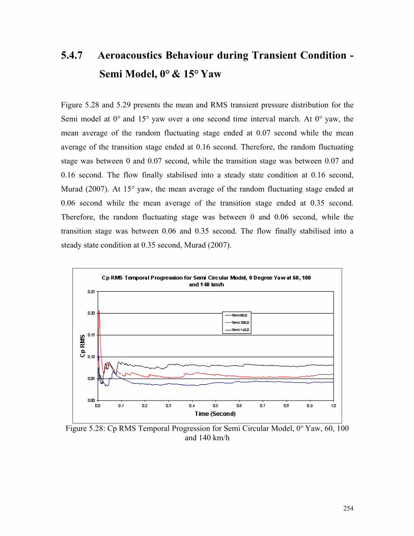
5.4.7 Aeroacoustics Behaviour during Transient Condition -
Semi Model, 0° & 15° Yaw
Figure 5.28 and 5.29 presents the mean and RMS transient pressure distribution for the
Semi model at 0° and 15° yaw over a one second time interval march. At 0° yaw, the
mean average of the random fluctuating stage ended at 0.07 second while the mean
average of the transition stage ended at 0.16 second. Therefore, the random fluctuating
stage was between 0 and 0.07 second, while the transition stage was between 0.07 and
0.16 second. The flow finally stabilised into a steady state condition at 0.16 second,
Murad (2007). At 15° yaw, the mean average of the random fluctuating stage ended at
0.06 second while the mean average of the transition stage ended at 0.35 second.
Therefore, the random fluctuating stage was between 0 and 0.06 second, while the
transition stage was between 0.06 and 0.35 second. The flow finally stabilised into a
steady state condition at 0.35 second, Murad (2007).
Figure 5.28: Cp RMS Temporal Progression for Semi Circular Model, 0° Yaw, 60, 100
and 140 km/h
254

Figure 5.29: Cp RMS Temporal Progression for Semi Circular Model, 15° Yaw, 60, 100
and 140 km/h
5.4.8 Aeroacoustics Behaviour during Transient Condition -
LE Model, 0° & 15° Yaw
Figure 5.30 and 5.31 presents the mean and RMS transient pressure distribution for the
Large Ellipsoidal model at 0° and 15° yaw over a one second time interval march. At 0°
yaw, the mean average of the random fluctuating stage ended at 0.02 second while the
mean average of the transition stage ended at 0.13 second. Therefore, the random
fluctuating stage was between 0 and 0.02 second, while the transition stage was between
0.02 and 0.13 second. The flow finally stabilised into a steady state condition at 0.13
second, Murad (2007). At 15° yaw, the mean average of the random fluctuating stage
ended at 0.04 second while the mean average of the transition stage ended at 0.26 second.
Therefore, the random fluctuating stage was between 0 and 0.04 second, while the
transition stage was between 0.04 and 0.26 second. The flow finally stabilised into a
steady state condition at 0.26 second, Murad (2007).
255

Figure 5.30: Cp RMS Temporal Progression for Large Ellipsoidal Model, 0° Yaw, 60,
100 and 140 km/h
Figure 5.31: Cp RMS Temporal Progression for Large Ellipsoidal Model, 15° Yaw, 60,
100 and 140 km/h
256

5.4.9 Aeroacoustics Behaviour during Transient Condition -
RE Model, 0° & 15° Yaw
Figure 5.32 and 5.33 presents the mean and RMS transient pressure distribution for the
RE model at 0° and 15° yaw over a one second time interval march. At 0° yaw, the mean
average of the random fluctuating stage ended at 0.05 second while the mean average of
the transition stage ended at 0.23 second. Therefore, the random fluctuating stage was
between 0 and 0.05 second, while the transition stage was between 0.05 and 0.23 second.
The flow finally stabilised into a steady state condition at 0.23 second. At 15° yaw, the
mean average of the random fluctuating stage ended at 0.06 second while the mean
average of the transition stage ended at 0.29 second. Therefore, the random fluctuating
stage was between 0 and 0.06 second, while the transition stage was between 0.06 and
0.29 second. The flow finally stabilised into a steady state condition at 0.29 second.
Figure 5.32: Cp RMS Temporal Progression for Rectangular Edge Model, 0° Yaw, 60,
100 and 140 km/h
257

Figure 5.33: Cp RMS Temporal Progression for Rectangular Edge Model, 15° Yaw, 60,
100 and 140 km/h
5.4.10 Aeroacoustics Behaviour during Transient
Condition - SL Model, 0° & 15° Yaw
Figure 5.34 and 5.35 presents the mean and RMS transient pressure distribution for the
Slanted Edge model at 0° and 15° yaw over a one second time interval march. At 0° yaw,
the mean average of the random fluctuating stage ended at 0.09 second while the mean
average of the transition stage ended at 0.34 second. Therefore, the random fluctuating
stage was between 0 and 0.09 second, while the transition stage was between 0.09 and
0.34 second. The flow finally stabilised into a steady state condition at 0.34 second. At
15° yaw, the mean average of the random fluctuating stage ended at 0.09 second while
the mean average of the transition stage ended at 0.50 second. Therefore, the random
fluctuating stage was between 0 and 0.09 second, while the transition stage was between
0.09 and 0.50 second. The flow finally stabilised into a steady state condition at 0.50
second.
258

Figure 5.34: Cp RMS Temporal Progression for Slanted Edge Model, 0° Yaw, 60, 100
and 140 km/h
Figure 5.35: Cp RMS Temporal Progression for Slanted Edge Model, 15° Yaw, 60, 100
and 140 km/h
259

5.4.11 CAA Behaviour & Distribution behind A-pillar Region
- SE Model, 0° Yaw
The results obtained showed that under steady condition, the OASPL magnitude on the
SE model surface at 0° yaw was measured at an average of 122.7-dB. As the aero
acoustics propagates away from the surface, the OASPL experienced a decrease of 2.1-
dB. From Figure 5.36, it can be seen that the two-dimensional trailing edge vortex region
propagating from the A-pillar base junction was measured at an average of 123.0-dB. The
two-dimensional attached turbulent boundary layer flow propagating from the A-pillar
apex propagated OASPL was measured at an average of 119.0-dB. Progressing
downstream of the flow, it can be seen from Figure 5.36 that the aero-acoustic
propagation due to the A-pillar base junction and A-pillar apex vortex remain close to the
surface of the vehicle while at the same time propagating sideways away from the A-
pillar base junction. From Figure 5.36, plan view of the aero-acoustic propagation shows
a reduction of 4-dB moving away from the A-pillar apex and base junction.
Under transient flow conditions, the initial OASPL magnitude on the model surface was
measured at an average of 119.5-dB (Figure 5.37). As the aero-acoustics propagation
reached steady state, it experienced an increase of 3.2-dB taking it to 122.7-dB. From
Figures 5.38 and 5.39 it can be seen that the aero-acoustic activity is continuous
propagating from the A-pillar base junction. However, the aero-acoustic propagation
from the A-pillar apex reached steady state after 0.1-second.
260

Figure 5.36: OASPL, Frontal and Surface View, Steady State Condition, Small
Ellipsoidal Model, 0° Yaw, 140 km/h
261

Figure 5.37: OASPL, Surface View, Transient Condition, Small Ellipsoidal Model, 0°
Yaw, 140 km/h
262

Figure 5.38: OASPL, Top View (Base), Transient Condition, Small Ellipsoidal Model, 0°
Yaw, 140 km/h
263
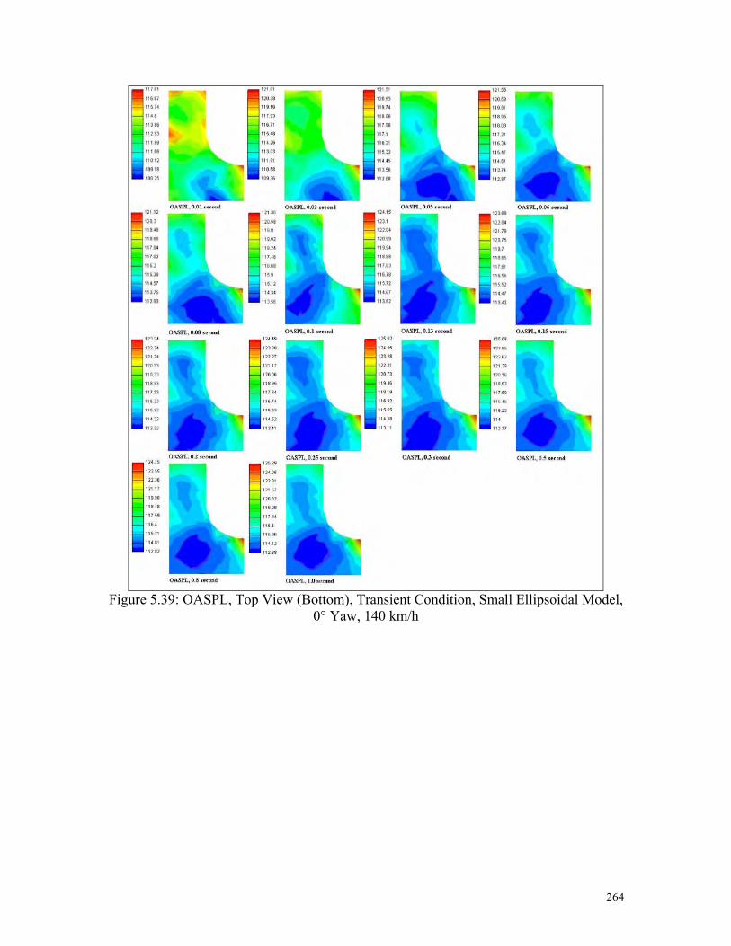
Figure 5.39: OASPL, Top View (Bottom), Transient Condition, Small Ellipsoidal Model,
0° Yaw, 140 km/h
264

5.4.12 CAA Behaviour & Distribution Behind A-
pillar Region - SE Model, 15° Yaw
The results obtained showed that under steady condition, the OASPL magnitude
on the SE model surface at 15° yaw was measured at an average of 123.0-dB. As
the aero acoustics propagates away from the surface, the OASPL experienced a
decrease of 4.5-dB. From Figure 5.40, it can be seen that the two-dimensional
trailing edge vortex region propagating from the A-pillar base junction was
measured at an average of 125.0-dB. The three-dimensional and three-
dimensional quasi-elongated helical from the A-pillar apex propagation was
measured at an average of 125.0-dB. From Figure 5.40, plan view of the aero-
acoustic propagation shows a reduction of 2.0-dB moving away from the A-pillar
apex and base junction.
Under transient flow conditions, the initial OASPL magnitude on the model
surface was measured at an average of 121.5-dB in the leeward region and 119.0-
dB in the windward region (Figure 5.41). As the aero-acoustics propagation
reached steady state, the leeward region experienced an increase of 1.5-dB and the
windward region experienced an increase of 3.5-dB. From Figures 5.42 and 5.43
it can be seen that the aero-acoustic activity is continuous propagating from the A-
pillar base junction and apex.
265

Figure 5.40: OASPL, Surface and Top View, Steady State Condition, Small
Ellipsoidal Model, 15° Yaw, 140 km/h
266

Figure 5.41: OASPL, Surface View (Leeward), Transient Condition, Small
Ellipsoidal Model, 15° Yaw, 140 km/h
267
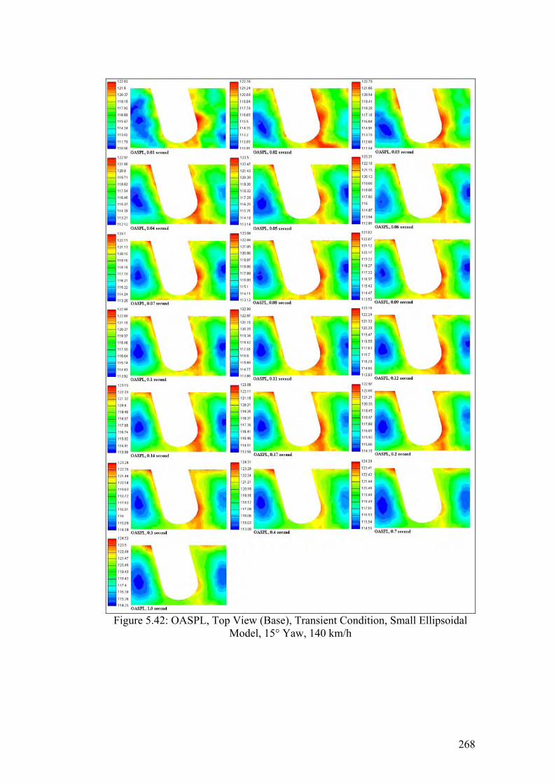
Figure 5.42: OASPL, Top View (Base), Transient Condition, Small Ellipsoidal
Model, 15° Yaw, 140 km/h
268

Figure 5.43: OASPL, Top View (Bottom), Transient Condition, Small Ellipsoidal
Model, 15° Yaw, 140 km/h
269

5.4.13 CAA Behaviour & Distribution Behind A-
pillar Region - Semi Model, 0° Yaw
The results obtained showed that under steady condition, the OASPL magnitude
on the Semi model surface at 0° yaw was measured at an average of 121.5-dB. As
the aero acoustics propagates away from the surface, the OASPL experienced a
decrease of 3.4-dB. From Figure 5.44, it can be seen that the two-dimensional free
trailing edge vortex region propagating from the A-pillar base junction was
measured at an average of 122.5-dB. The two-dimensional attached turbulent
boundary layer flow propagating from the A-pillar apex was measured at an
average of 117.0-dB. Progressing downstream of the flow, it can be seen from
Figure 5.44 that the aero-acoustic propagation due to the A-pillar base junction
and A-pillar apex vortex remain close to the surface of the vehicle while at the
same time propagating sideways away from the A-pillar base junction
experiencing a reduction of 2.0-dB.
Under transient flow conditions, the initial OASPL magnitude on the model
surface was measured at an average of 117.2-dB (Figure 5.45). As the aero-
acoustics propagation reached steady state, it experienced an increase of 4.3-dB
taking it to 121.5-dB. From Figures 5.46 and 5.47 it can be seen that the aero-
acoustic activity is continuous propagating from the A-pillar base junction,
reaching steady state after 0.1-second. The aero-acoustic propagation from the A-
pillar apex reached steady state after 0.02-second.
270

Figure 5.44: OASPL, Frontal and Surface View, Steady State Condition, Semi
Circular Model, 0° Yaw, 140 km/h
271

Figure 5.45: OASPL, Surface View, Transient Condition, Semi Circular Model,
0° Yaw, 140 km/h
272

Figure 5.46: OASPL, Top View (Base), Transient Condition, Semi Circular
Model, 0° Yaw, 140 km/h
273
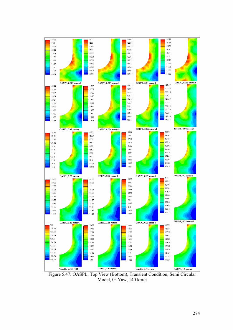
Figure 5.47: OASPL, Top View (Bottom), Transient Condition, Semi Circular
Model, 0° Yaw, 140 km/h
274

5.4.14 CAA Behaviour & Distribution Behind A-
pillar Region - Semi Model, 15° Yaw
The results obtained showed that under steady condition, the OASPL magnitude
on the Semi model surface at 15° yaw was measured at an average of 122.2-dB.
As the aero acoustics propagates away from the surface, the OASPL experienced
a decrease of 3.5-dB. From Figure 5.48, it can be seen that the two-dimensional
trailing edge vortex region propagating from the A-pillar base junction was
measured at an average of 123.0-dB. The three-dimensional and three-
dimensional quasi-elongated helical from the A-pillar apex propagation was
measured at an average of 123.0-dB. From Figure 5.48, plan view of the aero-
acoustic propagation shows a reduction of 3.0-dB moving away from the A-pillar
apex and base junction.
Under transient flow conditions, the initial OASPL magnitude on the model
surface was measured at an average of 120.5-dB in the leeward region and 118.9-
dB in the windward region (Figure 5.49). As the aero-acoustics propagation
reached steady state, the leeward region experienced an increase of 2.2-dB and the
windward region experienced an increase of 2.8-dB. From Figures 5.50 and 5.51
it can be seen that the aero-acoustic activity is continuous propagating from the A-
pillar base junction, reaching steady state condition after 0.05-second and behind
the A-pillar apex, reaching steady state condition after 0.2-second.
275
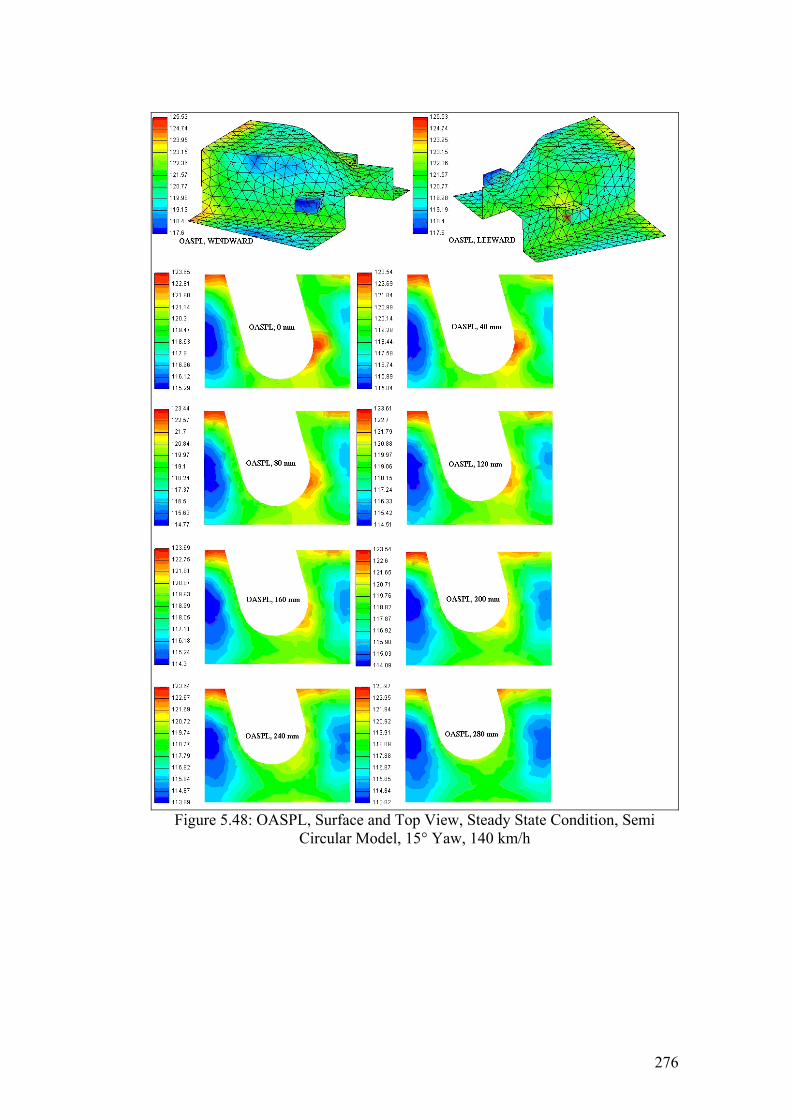
Figure 5.48: OASPL, Surface and Top View, Steady State Condition, Semi
Circular Model, 15° Yaw, 140 km/h
276

Figure 5.49: OASPL, Surface View (Leeward), Transient Condition, Semi
Circular Model, 15° Yaw, 140 km/h
277

Figure 5.50: OASPL, Top View (Base), Transient Condition, Semi Circular
Model, 15° Yaw, 140 km/h
278

Figure 5.51: OASPL, Top View (Bottom), Transient Condition, Semi Circular
Model, 15° Yaw, 140 km/h
279
5.4.15 CAA Behaviour & Distribution Behind A-
pillar Region - LE Model, 0° Yaw
The results obtained showed that under steady condition, the OASPL magnitude
on the LE model surface at 0° yaw was measured at an average of 120.8-dB. As
the aero acoustics propagates away from the surface, the OASPL experienced a
decrease of 4.2-dB. From Figure 5.52, it can be seen that the two-dimensional
trailing edge vortex region propagating from the A-pillar base junction was
measured at an average of 120.0-dB. The two-dimensional attached turbulent
boundary layer flow propagating from the A-pillar apex propagation was
measured at an average of 116.5-dB. Progressing downstream of the flow, it can
be seen from Figure 5.52 that the aero-acoustic propagation due to the A-pillar
base junction and A-pillar apex vortex remain close to the surface of the vehicle
while at the same time propagating sideways away from the A-pillar base
junction, experiencing a reduction of 1-dB.
Under transient flow conditions, the initial OASPL magnitude on the model
surface was measured at an average of 115.8-dB (Figure 5.53). As the aero-
acoustics propagation reached steady state, it experienced an increase of 5.0-dB
taking it to 120.8-dB. From Figures 5.54 and 5.55 it can be seen that the aero-
acoustic activity is continuous propagating from the A-pillar base junction,
reaching steady state condition after 0.02-second. However, the aero-acoustic
propagation from the A-pillar apex reached steady state after 0.08 second.
280

Figure 5.52: OASPL, Surface and Frontal View, Steady State Condition, Large
Ellipsoidal Model, 0° Yaw, 140 km/h
281
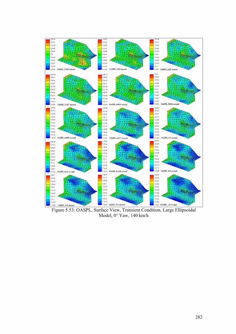
Figure 5.53: OASPL, Surface View, Transient Condition, Large Ellipsoidal
Model, 0° Yaw, 140 km/h
282

Figure 5.54: OASPL, Top View (Base), Transient Condition, Large Ellipsoidal
Model, 0° Yaw, 140 km/h
283
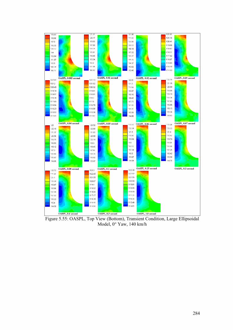
Figure 5.55: OASPL, Top View (Bottom), Transient Condition, Large Ellipsoidal
Model, 0° Yaw, 140 km/h
284
5.4.16 CAA Behaviour & Distribution Behind A-
pillar Region - LE Model, 15° Yaw
The results obtained showed that under steady condition, the OASPL magnitude
on the LE model surface at 15° yaw was measured at an average of 121.6-dB. As
the aero acoustics propagates away from the surface, the OASPL experienced a
decrease of 3.0-dB. From Figure 5.56, it can be seen that the two-dimensional
trailing edge vortex region propagating from the A-pillar base junction and the
three-dimensional and three-dimensional quasi-elongated helical from the A-pillar
apex propagation was measured at an average of 121.0-dB and 122.5-dB
respectively. From Figure 5.40, plan view of the aero-acoustic propagation shows
a reduction of 4-dB moving away from the A-pillar apex and base junction.
Under transient flow conditions, the initial OASPL magnitude on the model
surface was measured at an average of 120.0-dB in the leeward region and 118.7-
dB in the windward region (Figure 5.57). As the aero-acoustics propagation
reached steady state, the leeward region experienced an increase of 2.7-dB and the
windward region experienced an increase of 2.2-dB. From Figures 5.42 and 5.43
it can be seen that the aero-acoustic activity is continuous propagating from the A-
pillar base junction and apex, reaching steady state condition after 0.1-second.
The results obtained from the simulation showed that the acoustical intensity is
higher in region closer to the vehicle surface and decreases as it moves away from
the surface. Highest acoustical intensity occurs in the A-pillar region. As the
vehicle is yawed, acoustical intensity increases with time before it reaches steady
state condition. The leeward region, which experience a larger separation
compared to the windward region, produces a higher acoustical intensity. Finally,
the results show that steady state condition was reached only after 0.1-second.
After 0.1-second the overall vortex structure formation has fully evolved.
However, subtle turbulence unsteadiness within the vortex structure is will always
be present. The behaviour and distribution of the acoustical propagation in the
surrounding A-pillar region is a direct consequence to the formation of the A-
285
pillar vortex due to the geometrical characteristics of the vehicle A-pillar and
windshield radii and also due to the exposure to various yaw angle orientation.
286
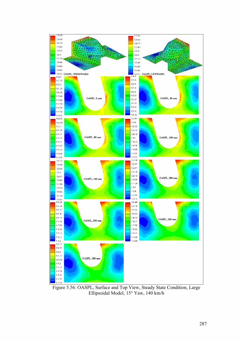
Figure 5.56: OASPL, Surface and Top View, Steady State Condition, Large
Ellipsoidal Model, 15° Yaw, 140 km/h
287
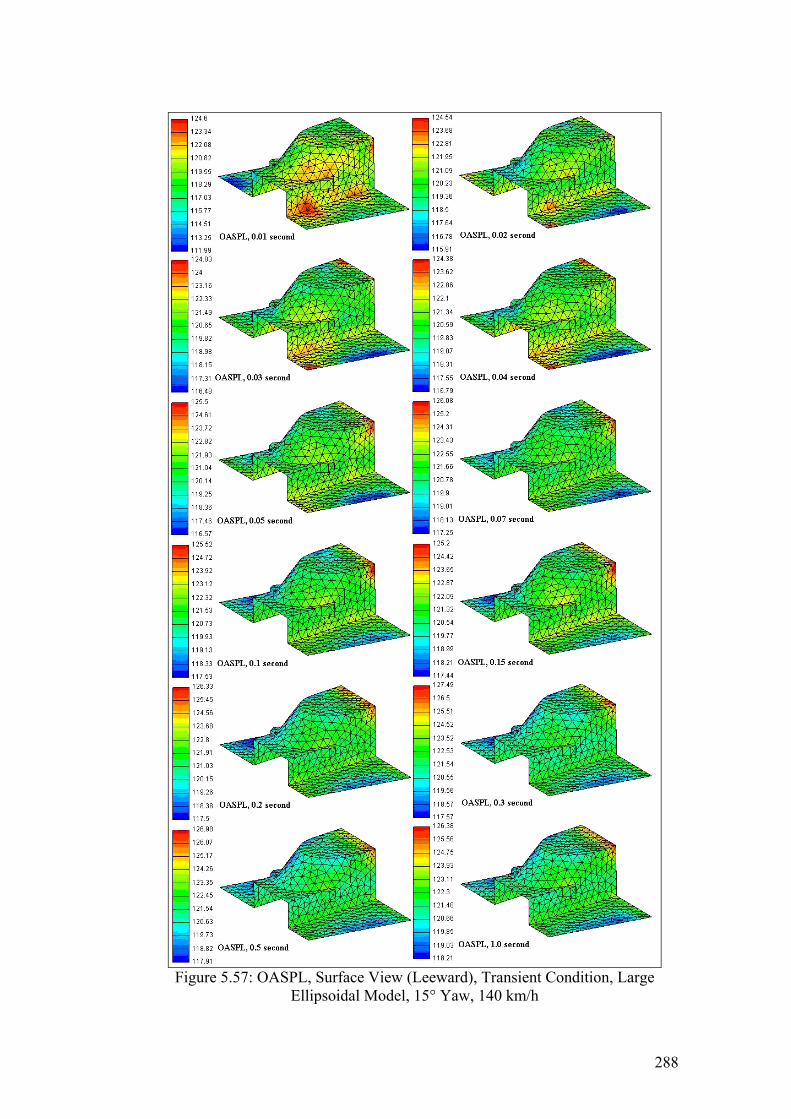
Figure 5.57: OASPL, Surface View (Leeward), Transient Condition, Large
Ellipsoidal Model, 15° Yaw, 140 km/h
288

Figure 5.58: OASPL, Top View (Base), Transient Condition, Large Ellipsoidal
Model, 15° Yaw, 140 km/h
289

Figure 5.59: OASPL, Top View (Bottom), Transient Condition, Large Ellipsoidal
Model, 15° Yaw, 140 km/h
290
5.5 Discussion of Hybrid SWIFT CAA Results
The discussion of results obtained from using hybrid SWIFT CAA modelling will
be presented in this section. Discussion of results will be divided into four sub-
sections. The first two sections discuss the comparison between the CAA and
experimental results. The third section discusses the transient behaviour of the
acoustical propagation while the final section discusses the overall acoustical
behaviour and distribution within the A-pillar region.
5.5.1 Comparison between Hybrid SWIFT CAA &
Experimental Results – Cp RMS Pressure
Hybrid SWIFT CAA results of Cp RMS distribution showed good correlation
when compared to results obtained by Alam (2000). The comparison of results
can be seen in Figures 5.2, 5.3, 5.7, 5.8, 5.11, 5.12, 5.16, 5.17, 5.18, 5.21, 5.22
and 5.23. The results were consistent with the findings of Murad (2007). The
results of Cp RMS distribution at various inlet velocities (60, 100 and 140 km/h)
collapsed into a single curve for each model. As per Alam (2000), the modelled
results showed that the airflow at various inlet velocities is Reynolds number
independent.
291

Figure 5.60: Comparison between Numerical and Experimental Results of Peak
Cp RMS for Reynolds Number Sensitivity, 0° Yaw
Figures 5.60, 5.61 and 5.62 showed the Reynolds number sensitivity of peak Cp
RMS. For all yaw angles, the variations of peak Cp RMS were small and the
results obtained from the CAA simulation correlates well with the results obtained
from Alam (2000). The maximum variation in CAA results obtained from circular
models at 0° yaw was 0.050 as compared to 0.025, obtained experimentally. At -
15° yaw, CAA results produced maximum variations of about 0.025, compared to
0.050, obtained experimentally. Finally, at +15° yaw, maximum variations
obtained from both CAA and empirical results were 0.020. The maximum
variation obtained from models with sharp edge models at 0° yaw was 0.20 as
compared to 0.28, obtained experimentally. At -15° yaw, CAA results produced
maximum variations of about 0.15, compared to 0.42, obtained experimentally.
Finally, at +15° yaw, CAA results produced maximum variations of about 0.07,
compared to 0.12, obtained experimentally. Discrepancies in the CAA results is
caused by the discrepancies obtained in the earlier CFD models (discussed in
Chapter 4) and also due to numerical discrepancies caused by the acoustical
model used in software to determine the acoustical propagation estimation. This
discrepancy in results is small and acceptable due to the constant fluctuating of
acoustical pressure prior conversion to Cp RMS values.
292
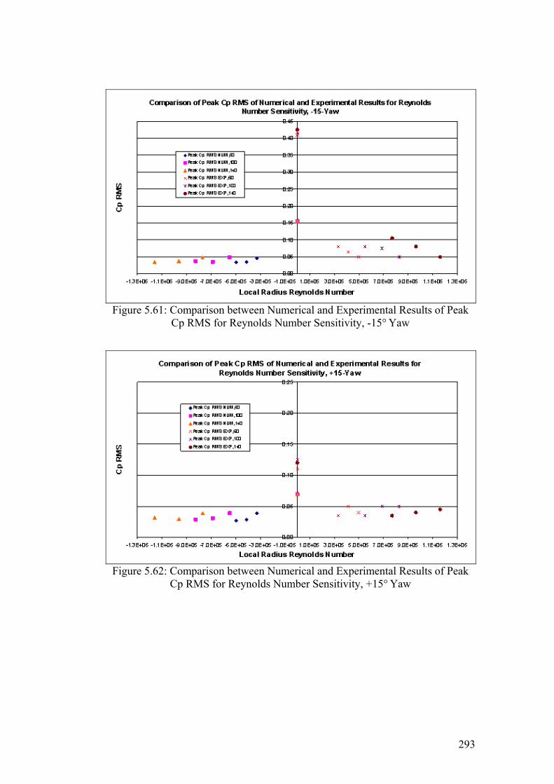
Figure 5.61: Comparison between Numerical and Experimental Results of Peak
Cp RMS for Reynolds Number Sensitivity, -15° Yaw
Figure 5.62: Comparison between Numerical and Experimental Results of Peak
Cp RMS for Reynolds Number Sensitivity, +15° Yaw
293
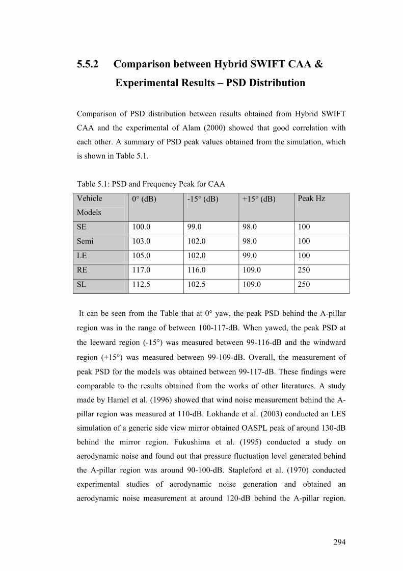
5.5.2 Comparison between Hybrid SWIFT CAA &
Experimental Results – PSD Distribution
Comparison of PSD distribution between results obtained from Hybrid SWIFT
CAA and the experimental of Alam (2000) showed that good correlation with
each other. A summary of PSD peak values obtained from the simulation, which
is shown in Table 5.1.
Table 5.1: PSD and Frequency Peak for CAA
Vehicle
Models
0° (dB) -15° (dB) +15° (dB) Peak Hz
SE 100.0 99.0 98.0 100
Semi 103.0 102.0 98.0 100
LE 105.0 102.0 99.0 100
RE 117.0 116.0 109.0 250
SL 112.5 102.5 109.0 250
It can be seen from the Table that at 0° yaw, the peak PSD behind the A-pillar
region was in the range of between 100-117-dB. When yawed, the peak PSD at
the leeward region (-15°) was measured between 99-116-dB and the windward
region (+15°) was measured between 99-109-dB. Overall, the measurement of
peak PSD for the models was obtained between 99-117-dB. These findings were
comparable to the results obtained from the works of other literatures. A study
made by Hamel et al. (1996) showed that wind noise measurement behind the A-
pillar region was measured at 110-dB. Lokhande et al. (2003) conducted an LES
simulation of a generic side view mirror obtained OASPL peak of around 130-dB
behind the mirror region. Fukushima et al. (1995) conducted a study on
aerodynamic noise and found out that pressure fluctuation level generated behind
the A-pillar region was around 90-100-dB. Stapleford et al. (1970) conducted
experimental studies of aerodynamic noise generation and obtained an
aerodynamic noise measurement at around 120-dB behind the A-pillar region.
294

Haruna et al. (1990) experimented using a production car in a wind tunnel, where
the OASPL level measured at around 110-dB at 0° yaw. Haruna et al. (1992)
developed a numerical model to estimate the distribution of surface pressure
fluctuation for aerodynamic noise prediction and found out that the highest
contributor of aerodynamic noise is the A-pillar with overall sound pressure level
ranging between 110-130-dB. Haruna et al. (1992) developed a numerical model
to analyze aerodynamic noise to mimic an A-pillar flow and found out that the
highest peak of predicted OASPL was obtained at 110-dB. Bergamini et al. (1997)
conducted both experimental and numerical simulation on an A-pillar bluff body
and obtained sound pressure level of 115-dB from experimental measurement and
135-dB from the numerical model. Strumolo et al. (1998) simulated external
aerodynamic noise to mimic the A-pillar region using CFD and obtained an
OASPL of 125-dB from CFD and 120-dB empirically. Kumarasamy et al. (1999)
conducted experimental and numerical simulation of A-pillar to predict
aerodynamic noise and obtained an OASPL of 100-dB from experimental and
130-dB from CFD simulation.
On average the peak OASPL obtained from the works conducted from the
literature was between 90-130-dB. The results obtained from Hybrid SWIFT
CAA was between 99-117-dB, which makes it comparable with existing
literatures. Discrepancies observed in the CAA results is caused by the
discrepancies earlier obtained in the CFD models (discussed in Chapter 4) and
also due to numerical error caused by the acoustical model used in software to
determine the acoustical propagation estimation.
From Table 5.1, frequency corresponding to the peak PSD was also obtained. It
can be seen that at peak PSD, the corresponding frequency was measured between
100-Hz to 250-Hz. According to Stapleford et al. (1970), Haruna et al. (1990) and
Hanaoka et al. (1993), the highest sound pressure level obtained in region of low
frequency was caused by large-scale turbulent structures at the area of flow
separation. This was observed from the previous chapter especially when vehicle
was exposed to a certain yaw angle. At low Mach number, this large-scale
295

turbulent structure changes the mean flow-field to produce low frequency pressure
fluctuation, Simpson (1987, 1989). George (1990) and Callister et al. (1998)
described this type of noise as broadband noise.
On average the dominant frequency level corresponding to the peak OASPL
obtained from the works conducted from the literature was between 100 to 500-
Hz. The results obtained from Hybrid SWIFT CAA was between 100 to 250-dB,
which makes it comparable with existing literatures. As with previous results,
discrepancies observed in the CAA results is caused by discrepancies obtained in
the CFD models (discussed in Chapter 4) and also due to numerical error caused
by the acoustical model used in software to determine the acoustical propagation
estimation. George (1995) stated that aerodynamic noise is dominant in frequency
region of between 500-Hz to 12,000-Hz. Buchheim et al. (1982) states A-pillar
noise corresponds to region of low frequency between 250-Hz to 500-Hz.
According to Haruna (1992) et al. the A-pillar noise corresponds to region of low
frequency between 100 to 500-Hz. A study made by Hamel et al. (1996), have
showed that the A-pillar region dominates the frequency spectrum range of lower
than 1000-Hz. Li et al. (2003) conducted experimental and numerical study on
reducing external aerodynamic noise and found out that peak sound pressure level
was measure at frequency region of between 250 to 500-Hz using experimental
method and between 500 to 1300-Hz using finite element method.
Table 5.2: PSD Peak and Overall Discrepancy between CAA and experimental
Peak Discrepancy (dB) Overall Discrepancy (dB) Vehicle
Models 0° -15° +15° 0° -15° +15° Average
SE 1.0 14.0 3.0 7.3 13.3 5.0 8.5
Semi 14.0 18.0 19.0 7.0 15.0 12.0 11.3
LE 5.0 13.0 15.0 3.0 6.8 10.0 6.6
RE 7.0 10.5 19.0 7.0 8.3 13.0 9.4
SL 10.5 26.5 7.0 15.3 17.0 5.3 12.5
296
The findings obtained using Hybrid SWIFT CAA (Figures 5.4, 5.5, 5.9, 5.13,
5.14, 5.19 and 5.24) showed that the PSD distributions for the models compared
to the experimental results were under predicted. The average discrepancy
between Hybrid SWIFT CAA and the experimental results were obtained and
collated in Table 5.2. Average discrepancy obtained for the models was measured
to be between 8.5-dB to 12.5-dB. Discrepancies observed in the CAA results is
caused by the discrepancies earlier obtained in the CFD models (discussed in
Chapter 4) and also due to numerical error caused by the acoustical model used in
software to determine the acoustical propagation estimation.
Discrepancy of overall mean PSD value was comparable to the results obtained
from the works of Lokhande et al. (2003), Ogawa et al. (1999), Uchida et al.
(1999), which showed overall mean PSD discrepancies of around 15.0-dB for
CAA modeling behind a bluff body region. Haruna et al. (1992) PSD analysis
against measured results for A-pillar modeling showed that the numerical results
were under predicted by about 20.0-dB, which was caused by insufficient amount
of grid generation. Bergamini et al. (1997) experimental and numerical simulation
in predicting aerodynamic noise of an A-pillar bluff body to predict vehicle
aerodynamic noise resulted an over prediction by 20.0-dB. Strumolo et al. (1998)
simulated external aerodynamic noise to mimic the A-pillar region using CFD
with an over prediction of results by about 5.0-dB. Kumarasamy et al. (1999)
experimental and numerical simulation of A-pillar to predict aerodynamic noise
showed an over prediction of peak PSD by 30.0-dB. Overall PSD showed an
under prediction by 10.0-dB. Li et al. (2003) conducted experimental and
numerical study on reducing external aerodynamic noise on an actual model of a
vehicle A-pillar with results showing a 5.0-dB to 10.0-dB over prediction.
On average the over/under prediction of PSD results obtained from the works
conducted from the literature was between 5.0-dB to 30.0-dB. The results
obtained from Hybrid SWIFT CAA showed an under prediction of between 8.5-
dB to 12.5-dB, which makes it comparable with existing literatures.
297

5.5.3 Aero-acoustics Behaviour during Transient
Conditions
The transient progression for each investigated scale model can be seen in Table
5.3. It can be seen based on the trend from the Table that the circular models
investigated will reach a faster transition (EP/ST) and steady state (ET/SS)
condition with increasing model windshield radii. This was observed when
models were yawed at both 0° and 15° yaw respectively. For sharp edge models,
faster transition and steady state were reached by the RE model as compared to
the SL model. Average time taken for models to reach transition and steady state
condition at 0° yaw was 0.06 and 0.21 seconds respectively. At 15° yaw, it took
the models an average time of 0.07 and 0.40 seconds to reach transition and
steady state condition respectively. It can be seen from the results obtained for the
aero-acoustic transient time march behaviour that both transition and steady state
condition were reached faster for models which does not experienced much
turbulence activities behind the A-pillar region and at un-yawed condition where
turbulent flow separation is less severe.
Table 5.3: Transient Progression of Aero-acoustics behind A-pillar Region EP/ST ET/SS Vehicle
Models 0° (second) 15° (second) 0° (second) 15° (second) SE 0.08 0.10 0.19 0.58 Semi 0.07 0.06 0.16 0.35 LE 0.02 0.04 0.13 0.26 RE 0.05 0.06 0.23 0.29 SL 0.09 0.09 0.34 0.50 Mean 0.06 0.07 0.21 0.40
Results from previous section have shown that for circular models, the LE model
experienced less turbulence activity behind its A-pillar region compared to the SE
model. This was due to the bigger windshield radius possessed by the LE model
encouraging attached flow with minimum turbulent boundary layer generation
throughout the A-pillar region downstream to the flow. Similar results obtained
from the previous section between the sharp edge models showing that due to the
298

slant angle configuration of the A-pillar, turbulence separation and vortex
generation behind the A-pillar is more prominent for the SL model causing the
flow needing a longer time before it reaches a much more stable quasi-steady state
condition.
Results from Table 5.3 also showed that the aero-acoustic time march propagation
behaviour is dependent on the type of flow separation or vortex generation that is
occurring behind the A-pillar region. At 0° yaw, it can be seen that the SE and SL
models reaches steady state at a similar time. However, aero-acoustic time march
propagation trend in Figures 5.26 to 5.35 shows that for the sharp edge model, the
time march propagation trend is occurring at a much higher Cp RMS level, which
indicate a different level of aero-acoustic activity experienced by the model
behind the A-pillar region. Flow separation and the type of vortex generated for
the circular and the sharp edge models at 0° yaw was different, which was shown
and discussed in the previous chapter. For the circular models at 0° yaw, type of
flow separation and vortex generated are from two distinct sources, namely the
base A-pillar junction and the A-pillar apex/roof junction respectively. These flow
separation and vortex generation are much weaker than the ones produced by the
sharp edge models at 0° yaw, which is three dimensional helical cone shaped
vortex and are much stronger in turbulence intensity. The time march aero-
acoustic propagation at 15° yaw between the circular and sharp edge model are
much more consistent and predictable since both experienced a similar type of
flow separation and vortex generation behind the A-pillar region due to the
yawing orientation. It can be seen that the SL model takes longer to reach steady
state condition as compared to the LE model due to the severity of the turbulence
activity experience behind its A-pillar region downstream to the flow.
It can be said that the determining factor for aero-acoustic time-march propagation
behaviour for the circular and sharp edge model are the geometrical configuration
of the A-pillar slant and windshield radii. This will then shape the intensity of the
flow separation and turbulence vortex generation occurring behind the A-pillar
region downstream to the flow. Although flow will reach a much stable steady
299
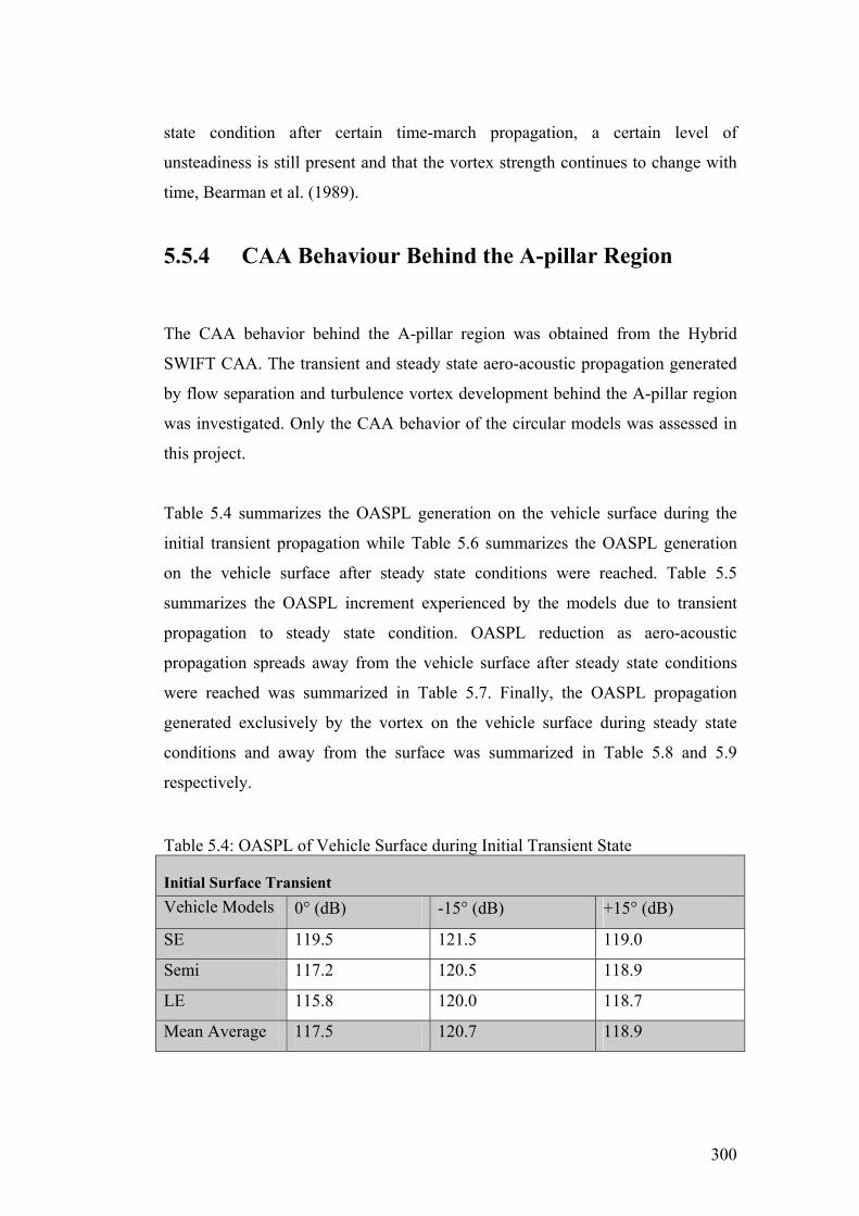
state condition after certain time-march propagation, a certain level of
unsteadiness is still present and that the vortex strength continues to change with
time, Bearman et al. (1989).
5.5.4 CAA Behaviour Behind the A-pillar Region
The CAA behavior behind the A-pillar region was obtained from the Hybrid
SWIFT CAA. The transient and steady state aero-acoustic propagation generated
by flow separation and turbulence vortex development behind the A-pillar region
was investigated. Only the CAA behavior of the circular models was assessed in
this project.
Table 5.4 summarizes the OASPL generation on the vehicle surface during the
initial transient propagation while Table 5.6 summarizes the OASPL generation
on the vehicle surface after steady state conditions were reached. Table 5.5
summarizes the OASPL increment experienced by the models due to transient
propagation to steady state condition. OASPL reduction as aero-acoustic
propagation spreads away from the vehicle surface after steady state conditions
were reached was summarized in Table 5.7. Finally, the OASPL propagation
generated exclusively by the vortex on the vehicle surface during steady state
conditions and away from the surface was summarized in Table 5.8 and 5.9
respectively. Table 5.4: OASPL of Vehicle Surface during Initial Transient State
Initial Surface Transient Vehicle Models 0° (dB) -15° (dB) +15° (dB)
SE 119.5 121.5 119.0
Semi 117.2 120.5 118.9
LE 115.8 120.0 118.7
Mean Average 117.5 120.7 118.9
300

Table 5.5: OASPL Increase from Transient to Steady on Vehicle Surface
OASPL Increase from Transient and Steady on Surface Vehicle Models 0° (dB) -15° (dB) +15° (dB)
SE 3.2 1.5 3.5
Semi 4.3 2.2 2.8
LE 5.0 2.7 2.2
Mean Average 4.2 3.0 2.8
Table 5.6: OASPL on Vehicle Surface during Steady State
Surface Steady Vehicle Models 0° (dB) -15° (dB) +15° (dB)
SE 122.7 123.0 122.5
Semi 121.5 122.7 121.7
LE 120.8 122.3 120.9
Mean Average 121.7 122.7 121.7
It can be seen from Table 5.4 and 5.6 that for the circular models, the OASPL
range were measured at between 115-121-dB during the initial transient state and
between 120-123-dB after it has reached steady state condition. On average the
OASPL obtained from the existing literatures are between 90-130-dB, which
makes the results obtained from Hybrid SWIFT CAA comparable with existing
literatures, Hamel et al. (1996), Lokhande et al. (2003), Fukushima et al. (1995),
Stapleford et al. (1970), Haruna et al. (1990), Haruna et al. (1992), Bergamini et
al. (1997), Strumolo et al. (1998), Kumarasamy et al. (1999).
Mean average obtained for the models during initial transient propagation and
after reaching steady state shows that OASPL magnitude are higher on the vehicle
surface during yaw conditions. There is a 3-dB difference during initial transient
propagation and a 1-dB difference during steady state condition when comparing
vehicles under yawed and un-yawed scenario. This finding is in agreement with
Haruna et al. (1990), in which stated that a difference up to 10-dB is present when
301

comparing OASPL magnitude between yawed and un-yawed vehicle. This finding
was also in agreement with Fricke (1968 and 1971) in which stated that wall
pressure fluctuations due to separated flow (which are more prominent at yaw
angles, discussed in the previous chapter) are higher than those beneath a
turbulent boundary layer (which are more prominent when vehicles are un-yawed,
as discussed in the previous chapter). This high level of flow separation at yaw
angle generates aerodynamic noise dipole effect, which is created due to the
unsteady high pressure force fluctuation impingement on the wall surface,
Hanaoka et al. (1993) and Callister et al. (1998).
It can be seen from Tables 5.4 and 5.6 as the windshield radii became larger, the
OASPL magnitude at 0° yaw decreases by 3.7-dB during initial transient
condition and 1.9-dB during steady state condition. At 15° yaw, the leeward
region experienced a decrease in OASPL magnitude as the windshield radii
becomes larger (1.5-dB reduction during initial transient condition and 0.7-dB
reduction during steady state condition). In the windward region, the OASPL
magnitude also experienced a decrease as the windshield radii become bigger
(0.3-dB reduction during initial transient condition and 1.6-dB reduction during
steady state condition). Overall, it can be seen from this finding that as the
OASPL magnitude decreases with increases windshield radii. This finding is in
agreement with Dobrzynski et al. (1994), Callister et al. (1998) and Alam (2000).
From Table 5.5, the models at 0° yaw experienced the largest increase in OASPL
magnitude (4.2-dB) as it propagates from the initial transient condition to steady
state condition. This is followed by the leeward (3.0-dB) and the windward (2.8-
dB) region respectively when the vehicles are positioned to 15° yaw angle. As the
windshield radii increases, the increase in OASPL magnitude as it propagates
from initial transient condition to steady states increases as well.
302
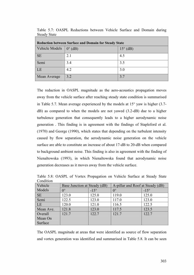
Table 5.7: OASPL Reductions between Vehicle Surface and Domain during Steady State
Reduction between Surface and Domain for Steady State Vehicle Models 0° (dB) 15° (dB)
SE 2.1 4.5
Semi 3.4 3.5
LE 4.2 3.0
Mean Average 3.2 3.7
The reduction in OASPL magnitude as the aero-acoustics propagation moves
away from the vehicle surface after reaching steady state condition is summarised
in Table 5.7. Mean average experienced by the models at 15° yaw is higher (3.7-
dB) as compared to when the models are not yawed (3.2-dB) due to a higher
turbulence generation that consequently leads to a higher aerodynamic noise
generation . This finding is in agreement with the findings of Stapleford et al.
(1970) and George (1990), which states that depending on the turbulent intensity
caused by flow separation, the aerodynamic noise generation on the vehicle
surface are able to constitute an increase of about 17-dB to 20-dB when compared
to background ambient noise. This finding is also in agreement with the finding of
Nienaltowska (1993), in which Nienaltowska found that aerodynamic noise
generation decreases as it moves away from the vehicle surface.
Table 5.8: OASPL of Vortex Propagation on Vehicle Surface at Steady State Condition
Base Junction at Steady (dB) A-pillar and Roof at Steady (dB) Vehicle Models 0° -15° 0° -15° SE 123.0 125.0 119.0 125.0 Semi 122.5 123.0 117.0 123.0 LE 120.0 121.0 116.5 122.5 Mean Ave. 121.8 123.0 117.5 123.5 Overall Mean On Surface
121.7 122.7 121.7 122.7
The OASPL magnitude at areas that were identified as source of flow separation
and vortex generation was identified and summarised in Table 5.8. It can be seen
303

from the Table that the average OASPL magnitude is higher at 15° yaw as
compared to 0° yaw. It can also be seen that the average OASPL magnitude is
much higher at the A-pillar base junction as compared to A-pillar and roof
junction for the circular models. In addition, it can be seen that the OASPL
magnitude on areas of vortex propagation decreases as the windshield radii of the
models increases for both at 0° and 15° yaw. There is a 4.3-dB difference between
OASPL magnitude at the A-pillar base junction as compared to the A-pillar apex
and roof junction at 0° yaw. At 15° yaw, the difference between the OASPL
magnitude at the A-pillar base junction as compared to the A-pillar apex and roof
junction is much smaller at 0.5-dB. Overall, mean surface OASPL magnitude
behind the A-pillar region combined (A-pillar Base Junction, A-pillar apex and
Roof) are higher compared to the overall mean OASPL magnitude on the surface
of the vehicle. This is in agreement with the findings of Stapleford et al. (1970)
and Strumolo et al. (1998).
It can be seen from Table 5.8 that the average OASPL magnitude on the A-pillar
base junction is slightly higher compared to the overall OASPL mean on the
surface of the models. At the A-pillar apex and roof junction, the overall OASPL
mean on the surface is higher at 0° yaw but smaller at 15° yaw.
Table 5.9: OASPL Reductions between Vehicle Surface and Domain during Steady State at Vortex propagation area
Base Junction/A-pillar/Roof Reduction at Steady (dB)Vehicle Models
0° -15°
SE 4.0 2.0
Semi 2.0 3.0
LE 1.0 4.0
Mean Average 2.3 3.0
The reduction in OASPL magnitude at the vortex propagation area as the aero-
acoustics propagation moves away from the vehicle surface after reaching steady
304

state condition is summarised in Table 5.9. Results show an average of between
1.0-dB to 4.0-dB increase comparing OASPL values between surface and CAA
domain. A higher surface and CAA domain difference is detected when the
vehicle is yawed (3.0-dB mean average difference as compared to 2.3-dB when
not yawed) as aerodynamic generation is higher. This finding is in agreement with
the findings of Stapleford et al. (1970) and George (1990), which states that
depending on the turbulent intensity caused by flow separation, the aerodynamic
noise generation on the vehicle surface are able to constitutes an increase to about
17-dB to 20-dB when compared to background ambient noise. This finding is also
in agreement with the finding of Nienaltowska (1993), in which Nienaltowska
found that aerodynamic noise generation decreases as it moves away from the
vehicle surface.
305

Chapter Six
CONCLUSIONS & RECOMMENDATIONS 6.1 Conclusions from Chapter 4
The development of the CFD and CAA model consists of a four-stage
process, in which, the first step was to first investigate and select the best
grids configurations for both the circular and sharp edge A-pillar models at
various respective yaw angles. The second and third stage process was to
select the best turbulence and near wall model for the final CFD model.
Turbulence and near wall models selected for comparison were taken from
different commercial CFD software’s FLUENT and SWIFT AVL. The
final stage in the development of the numerical model was to develop a
CAA model for the aero-acoustics modelling.
The grid configuration selected for this project was polyhedral grids from
SWIFT AVL. The total element count after final refinement was within an
acceptable limit of less than two million grids.
For the circular models (SE, Semi and LE) at 0°, the final turbulence and
NWM chosen for the project was the standard k – ε turbulence model with
the NWM of Chieng and Launder (1980).
For the circular models at 5°, 10° and 15° yaw angles, together with the
sharp edge models at 0°, 5°, 10° and 15° yaw, the final turbulence and
NWM model chosen for the project was the RSM with the WEB NWM of
Manceau and Hanjalic (2002).
Validation of the final CFD model against the experimental data of Alam
(2000) resulted in good correlations with mean error deviation obtained
within the acceptable recommended value of 20%.
The CAA model developed for this project resulted in a total grid count of
around 35,000 grids for the selected CAA domain. Final CAA modelling
was conducted using SWIFT CAA and assessment for aero-acoustics
306

behaviour behind the A-pillar region was conducted only for the circular
models due to their better correlations with experimental data.
Comparison of mean Cp values between the CFD and experimental results
in this chapter have shown that error of deviation for the circular models
(SE, Semi and LE) have all fallen within the recommended 20% margin.
The best performing model was the SE model at 0° which yielded an under
prediction of 8.2%. The worse performing model was the LE model at 15°
yaw which yielded an under prediction of 24.5%. For sharp edge models
(RE and SL) error of deviation for models at yaw angles of 0°, 5°, 10° and
15° yaw has also fallen within the recommended 20% margin. The best
performing model was the RE model at 0° which yielded an under
prediction of 11.9%. The worse performing model was the SL model at 0°
yaw which yielded an under prediction of 29.8%.
The size of the vortex measured for the various models at different yaw
angles in the leeward region of the flow suggest that with the circular
models (SE, Semi and LE) and the sharp edge models (RE and SL), the
vortex size increases with yaw angles.
Vortex for the circular models at 40% scale was measured between
115mm to 340mm in the horizontal component and between 102mm to
430mm in the vertical component. Vortex measurement for the circular
models at 40% scale shows that as the yaw angle increases from 0° to 15°
yaw, the vortex experiences a size increment of 225 mm in the horizontal
component and 328 mm in the vertical component.
Vortex for the RE model at 40% scale was measured between 80mm to
450mm in the horizontal component and between 200mm to 590mm in the
vertical component. Vortex measurement for the RE model at 40% scale
shows that as the yaw angle increases from 0° to 15° yaw, the vortex
experiences a size increment of 370 mm in the horizontal component and
390 mm in the vertical component.
Vortex for the SL model at 40% scale was measured between 110mm to
440mm in the horizontal component and between 360mm to 380mm in the
vertical component. Vortex measurement for the SL model at 40% scale
307
shows that as the yaw angle increases from 0° to 15° yaw, the vortex
experiences a size increment of 330 mm in the horizontal component and
60 mm in the vertical component.
The results obtained from the CFD analysis shows that for both the
circular and sharp edge models, the source of vortex separation behind the
A-pillar region originated from the junction of the A-pillar base, the A-
pillar apex and the front side window and roof junction. The mechanism of
flow separation for both the circular and sharp edge models was due to
trailing edge separation.
For circular models, the shape of the vortices that takes place at 0° yaw
took a physical form of a two-dimensional quasi-elongated oval. At 15°
yaw, the shape of the vortices for the circular models took an overall
physical form of a three-dimensional mixture of a quasi circular and cone
shaped helical vortex, which was a chaotic combination of two-
dimensional and three dimensional vortices originating from the A-pillar
base junction, apex and roof junction.
For the RE sharp edge model, shape of the vortex that takes place at 0°
yaw took a physical form a mixture of two-dimensional free trailing vortex
originated from the base of the A-pillar junction, while vortex generated
from the A-pillar apex formed a mixture of three-dimensional quasi
circular and cone shape helical vortex. The vortex generated from the roof
junction formed a three-dimensional circular shape vortex. All three form
of vortices flowed in stream wise direction, downstream to the flow. For
the RE shape edge model at 15° yaw, the shape of the vortex that takes
place at the A-pillar base junction and A-pillar apex was similar to that at
0° yaw.
For the SL sharp edge model, shape of the cortex that takes place at 0° yaw
took a physical form of a three-dimensional vertically elongated cone
shape helical vortex propagating downstream to the flow. At 0° yaw and
15° yaw, the shape of the vortex at the A-pillar base junction, the A-pillar
slant edge and the roof junction combine to form the three dimensional
308

conical helical vortex, making the turbulent intensity stronger as the yaw
angle increases.
Observation of various shapes of windshield radii and slant angle models
simulated in this project showed that the various geometrical
configurations of the windshield radii and slant angle governs the
behaviour pattern of vortex generation behind the A-pillar region when
exposed to yawed or un-yawed position. The observations have showed
that the vortex generated behind the A-pillar region was lower in intensity
and size in the circular models as compared to the sharp edge models. The
circular shape models windshield geometrical configuration and slant
angle created three different vortex formations, which shape the direction
of flow. The vortex generated from the various sources created a scenario
whereby the airflow path interferes with each other, creating a chaotic
quasi-circular vortex structure that prevents the formation of highly intense
vortices behind the A-pillar region. The sharp edge models windshield
geometrical configuration and slant angle created a scenario whereby the
airflow path from various directions converges together effectively to form
a highly intense three-dimensional helical cone shape vortex all the way
downstream to the flow. This produces region of high turbulent intensity
behind the A-pillar region. When subjected to yaw angles, the airflow
change angle of attack causes early turbulent boundary layer transition,
which will increase the vortex magnitude, and intensity further, which was
shown in the increase in the formation and size of the vortex.
309

6.2 Conclusions from Chapter 5
Hybrid SWIFT CAA results of Cp RMS distribution showed good
correlation when compared to results obtained by Alam (2000). The results
of Cp RMS distribution at various inlet velocities (60, 100 and 140 km/h)
showed good correlation with the existing experimental results of Alam
(2000).
On average the peak OASPL obtained from the works conducted from the
literature was between 90-130-dB. The results obtained from Hybrid
SWIFT CAA was between 99-117-dB, which makes it comparable with
existing literatures. The average discrepancy between Hybrid SWIFT
CAA and the experimental results for PSD distributions was measured to
be between 8.5-dB to 12.5-dB. On average the over/under prediction of
PSD results obtained from the works conducted from the literature was
between 5.0-dB to 30.0-dB, which makes it comparable with existing
literatures.
On average the dominant frequency level corresponding to the peak
OASPL obtained from the works conducted from the literature was
between 100 to 500-Hz. The results obtained from Hybrid SWIFT CAA
was between 100 to 250-dB, which makes it comparable with existing
literatures. The highest sound pressure level obtained in region of low
frequency at low Mach number was caused by large-scale turbulent
structures at the area of flow separation. The large-scale turbulent structure
changes the mean flow-field to produce low frequency pressure
fluctuation, which is often described as broadband noise.
The transient progression for each investigated scale model shows that the
circular models investigated will reach a faster transition (EP/ST) and
steady state (ET/SS) condition with increasing windshield radii and also
when not exposed to yaw condition. This is because as models windshield
radii increases, aerodynamic flow behind the A-pillar region experiences
less turbulence activities. Similar explanation is valid for models that are
not yawed. For sharp edge models, faster transition and steady state were
310

reached by the RE model as compared to the SL model. Turbulence
separation and vortex generation behind the A-pillar is more prominent for
the SL model causing the flow needing a longer time before it reaches a
much more stable quasi-steady state condition. Average time taken for
models to reach transition and steady state condition at 0° yaw was 0.07
and 0.40 seconds respectively. At 15° yaw, it took the models an average
time of 0.06 and 0.21 seconds to reach transition and steady state condition
respectively. Although flow will reach a much stable steady state condition
after certain time-march propagation, a certain level of unsteadiness is still
present and that the vortex strength continues to change with time.
For the circular models, the OASPL range on the surface were measured at
between 115-121-dB during the initial transient state and between 120-
123-dB after it has reached steady state condition. On average the OASPL
obtained from the existing literatures are between 90-130-dB, which
makes the results obtained from Hybrid SWIFT CAA comparable with
existing literatures.
As models propagates from the initial transient condition to steady state
condition, models at 0° yaw experienced the largest increase in OASPL
magnitude (4.2-dB). This is followed by the leeward (3.0-dB) and the
windward (2.8-dB) region respectively when the vehicles are positioned to
15° yaw.
Results show that OASPL magnitude is higher on the vehicle surface
during yaw conditions. There’s a 3-dB difference during initial transient
propagation and a 1-dB difference during steady state condition when
comparing vehicles under yawed and un-yawed scenario. This results is
comparable with existing literatures which stated that a difference up to
10-dB is present when comparing OASPL magnitude between yawed and
un-yawed vehicle.
Results also show that OASPL magnitude on the vehicle surface decreases
with increases windshield radii. This finding is in agreement with the
existing literatures. As the windshield radii becomes bigger, the OASPL
magnitude at 0° yaw decreases by 3.7-dB during initial transient condition
311
and 1.9-dB during steady state condition. At 15° yaw, the leeward region
experienced a decrease in OASPL magnitude as the windshield radii
becomes larger (1.5-dB reduction during initial transient condition and
0.7-dB reduction during steady state condition). In the windward region,
the OASPL magnitude also experienced a decrease as the windshield radii
become bigger (0.3-dB reduction during initial transient condition and 1.6-
dB reduction during steady state condition).
This findings shows that aerodynamic noise generation decreases as it
moves away from the vehicle surface. The reduction in OASPL magnitude
as the aero-acoustics propagation moves away from the vehicle surface
after reaching steady state condition shows that the mean average
experienced by the models at 15° yaw is higher (3.7-dB) as compared to
when the models are not yawed (3.2-dB). This finding is in agreement with
existing literatures, in which shows that the aerodynamic noise generation
on the vehicle surface are able to constitutes an increase to about 17-dB to
20-dB when compared to background ambient noise.
Overall, mean surface OASPL magnitude at the vortex source region (A-
pillar Base Junction, A-pillar apex and Roof) is slightly higher compared
to the overall mean OASPL magnitude on the surface of the vehicle. This
is in agreement with the findings of existing literatures.
There is a 4.3-dB difference between OASPL magnitude at the A-pillar
base junction as compared to the A-pillar apex and roof junction at 0° yaw.
At 15° yaw, the difference between the OASPL magnitude at the A-pillar
base junction as compared to the A-pillar apex and roof junction is much
smaller at 0.5-dB.
The reduction in OASPL magnitude at the vortex propagation area as the
aero-acoustics propagation moves away from the vehicle surface after
reaching steady state condition shows an average of between 1.0-dB to
4.0-dB increase comparing OASPL values between surface and CAA
domain. This finding is in agreement with the existing literatures, which
states that depending on the turbulent intensity caused by flow separation,
the aerodynamic noise generation on the vehicle surface are able to
312

constitutes an increase to about 17-dB to 20-dB when compared to
background ambient noise.
This PhD project has achieved its aim and objectives. The PhD research project of
Alam was extended. Using CFD approach the visualization of the vortex structure
behind the A-pillar region was modeled and investigated. The size and structure
of the vortex that was developed from various A-pillar windshield radii exposure
at various yaw angles was investigated and quantified. This was not achieved by
Alam using the experimental approach. The mechanism of A-pillar vortex
generation, the transient and also acoustical behaviour was also investigated in
this project and understood. The main achievement of this project is in the
development of methodology in the understanding the aerodynamic and aero
acoustic behaviour behind the A-pillar region of a vehicle. This study will be
beneficial to the automotive industries in the reduction of air borne noise for
passenger comfort. Further recommendation for future study is outline below.
6.3 Further Recommendations
Below are some of the recommendations for future work that were not included in
this project. The recommendations are as follows:
The aero acoustics pattern of behaviour and distribution on the model
surface and the surrounding CAA domain was investigated in this project
through the generation of OASPL. The scope of this project however
serves only as a ground work study for the aero acoustics modelling within
the vehicle A-pillar domain. However, it is recommended that further
validation to be conducted which includes empirical validation of the
model to identify proper mechanism of aero acoustics generation, i.e.
monopole or dipole type generation. It is also recommended that further
refinement can be conducted that includes grid independency testing for
the CAA domain to determine the most optimum grids that are required
for each CAA domain model. Apart from discrepancies caused by earlier
CFD models (discussed in Chapter 4) and also due to numerical error
313

caused by the acoustical model used in software to determine the
acoustical propagation estimation, lack of grid refinement of the CAA
domain might also contributed to the discrepancies caused.
The scope of this project was to use steady state RANS CFD results as
boundary conditions for the CAA modelling. Transient RANS CFD
modelling was not conducted due to time constraints in finishing this
project and it is recommended for future work in order to investigate and
analyse qualitatively the A-pillar vortex behaviour under transient
condition. In conducting transient modelling of the A-pillar aerodynamics,
it is recommended that LES modelling is used as it offers a higher level of
modelling accuracy without having to resort to extreme grid generation
capacity.
This scope of this project was limited to investigate and analyse generally
and qualitatively the pattern of behaviour of the A-pillar aerodynamics,
specifically the mechanism and formation of the A-pillar vortex at various
yaw angles and at various windshield radii. The behaviour within the
turbulence boundary layer separation was not carried out due to time
constraints and is still unknown. It is recommended for future works that
that a more detailed investigation be carried out on boundary layer
behaviour behind the A-pillar region in order to investigate the turbulence
unsteadiness and physics underneath the boundary layer separation. This
can be done by investigating the Reynolds stress behaviour within the
boundary layer flow in trying to find any correlation with acoustical
generation and propagation.
314
REFERENCES Affenzeller, J. and Rust, A., “Community Noise Research Strategy Plan”, Noise Technology Status Report for CALM Team, Europe, 2003. Ahmed, S.R., “A Survey of Automobile Aeroacoustics Activities in Germany”, SAE Paper, No 950623, 1995. Ahmed, S.R., “Computational Fluid Dynamics”, Chapter XV in Hucho, W.H (Ed.), Aerodynamics of Road Vehicles, 4th Edition, SAE International, Warrendale, PA, USA, 1998. Alam, F., “The Effects of Car A-Pillar and Windshield Geometry and Yaw Angles on Local Flow and Noise”, Ph.D. Thesis, Department of Mechanical and Manufacturing Engineering, RMIT University, Melbourne, Australia, 2000. Alam, F., Watkins, S., Song, B., Steiner, T. and Humphris, C., “The Flow Around a Car A-pillar”, The 13th Australasian Fluid Mechanics Conference, Melbourne, Australia, PP 461-464, 1998. American Heritage® Dictionary of the English Language (2000) Anderson, J.D. Jr., “Computational Fluid Dynamics: The Basics with Applications”, McGraw Hill, 1995. Atkins, H.L. and Shu, C.W., “Quadrature-Free Implementation of Discontinuous Galerkin Method for Hyperbolic Equations”, AIAA Journal, Vol 36, No 5, PP 775-782, 1998. Atkins, H.L. and Shu, C.W., “Quadrature-free Implementation of Discontinuous Galerkin Method for Hyperbolic Equations”, AIAA Journal, Vol. 36, PP 775-782, 1998. AVL SWIFT, AVL User Manual, Version 3.1, Austria, 2003. Baldwin, B.S. and Barth, T.J., “A One-Equation Turbulence Transport Model for High Reynolds Number Wall-Bounded Flows”, NASA TM-102847, 1990. Baldwin, B.S. and Lomax, H., “Thin-layer Approximation and Algebraic Model for Separated Turbulent Flows”, AIAA Paper, No 78-257, 1978. Barnard, R.H., “Road Vehicle Aerodynamic Design-An Introduction”, 2nd Edition, Longman ISBN 0-582-24522-2, 1996. Basara, B. and Jakirlic, S., “A New Turbulence Modeling Strategy for Industrial CFD”, International Journal of Numerical Methods in Fluids, Vol. 42, PP 89-116, 2003.
315

Basara, B. and Jakirlic, S., “A New Turbulence Modeling Strategy For Industrial CFD”, International Journal in Numerical Methods in Fluids, Vol. 42, PP 89-116, 2003. Bearman, P.W., De Beer, D. and Harvey, J.K., “Experimental Studies of Road Vehicle Flow Fields”, AIAA, Paper 89-1887, PP 1-9, 1989. Bechera, W., Lafon, P. and Bailly, C., “Application of a k-ε turbulence model to the prediction of noise for simple and coaxial free jets”, Journal of the Acoustic Society of America, Vol 97, No 6, PP 3518-3531, 1955. Bechera, W., Lafon, P., Bailly, C. and Candel, S., “Application of a k-ε Turbulence Model to the Prediction of Noise From Simple and Co-Axial Free Jets”, Journal of Acoustical Society of America, Vol. 97, No. 6, PP 3518-3531, 1996. Bergamini, P., Casella, M. and Vitali, D.F., “Computational Prediction of Vehicle Aerodynamic Boise by Integration of a CFD Technique with Lighthill’s Acoustic Analogy”, SAE Paper, No 970401, 1997. Boussinesq, J., “Essai sur la Theorie des eaux Courantes”, Mem. Pres. Par Div. Savant a l’Acad. Sci., 23, PP 1-680, 1877. Bradshaw, P., “Effects of Streamline Curvature on Turbulent Flow”, AGARD-AG-169, 1973. Bradshaw, P., “The Response of a Constant-Pressure Turbulent Boundary Layer to the Sudden Application of an Adverse Pressure Gradient”, R. & M. Number 3575, British Aeronautical Research Council, 1969. Bradshaw, P., Ferriss, D.H. and Atwell, N.P., “Calculation of Boundary Layer Development Using the Turbulent Energy Equation”, Journal of Fluid Mechanics, Vol. 28, Pt. 3, PP 593-616, 1967. Bremner, P.G. and Zhu, M., “Recent Progress using SEA and CFD to Predict Interior Wind Noise”, SAE Paper, No 2003-01-1705, 2003. Buchheim R.W., Dobrzynski, H., Mankau, H. and Schwabe, D., “Vehicle Interior Noise Related to External Aerodynamics”, International Journal of Vehicle Design, Special Publication SP3, PP 197-209, 1968. Buchheim R.W., Dobrzynski, H., Mankau, H. and Schwabe, D., “Vehicle Interior Noise Related to External Aerodynamics”, International Journal of Vehicle Design, Vol 3, No 4, PP 398-410, 1982.
316

Buchheim, R., Dobrzynski, W., Mankau, H. and Schwabe, D., “Vehicle Interior Noise Related to External Aerodynamics”, International Journal of Vehicle Design, Vol 3, No. 4, PP 398-410, U.K., 1982. Buley, M.D., “Industrial Noise Control”, Swinburne University of Technology Lecture Notes, School of Mechanical and Manufacturing Engineering, Swinburne University of Technology, Melbourne Australia, 1997. Callister, J.R. and George, A.R., “Wind Noise”, Chapter VIII in Hucho, W.H (Ed.), Aerodynamics of Road Vehicles, 4th Edition, SAE International, Warrendale, PA, USA, 1998. Cebeci, T. and Smith, A.M.O., “Analysis of Turbulent Boundary Layers”, Ser, in Applied Mathematics and Mechanics, Vol 15, Academic Press, 1974. CFD-Online Forum, Private Communication, 2002. Chen, H.C. and Patel, V.C., “Near Wall Turbulence Models for Complex Flows Including Separation”, AIAA Journal, 26(6), PP 641-648, 1988. Chien, K.Y., “Predictions of Channel and Boundary Layer Flows with a Low Reynolds Number Turbulence Model”, AIAA Journal, Vol. 20, No. 1, PP 33-38, 1982. Chieng, C.C. and Launder, B.E., “On the Calculation of Turbulent Heat Transport Downstream from an Abrupt Pipe Expansion”, Numerical Heat Transfer, Vol. 3, PP 189-207, 1980. Chou, P.Y., “On the Velocity Correlations and the Solution of the Equations of Turbulent Fluctuation”, Quart. Appl. Math., Vol. 3, PP 38, 1945. Clauser, F.H., “The Turbulent Boundary Layer”, Advances in Applied Mechanics, Vol. IV, Academic Press, PP 1-51, 1956. Coles, D.E. and Hirst, E.A., “Computing of Turbulent Boundary - 1968 AFOSR-IFP-Stanford Conference, Vol. II, Thermosciences Division, Stanford University, California, 1969. Corrsin, S. and Kistler, A.L., “The Free-Stream Boundaries of Turbulent Flows”, NACA TN 3133, 1954. Curle, N., “The Influence of Solid Boundaries on Aerodynamic Sound”, Proceedings of Royal Society, London, Series A, Vol 231, No 1187, PP 505-514, 1955. Daly, B.J. and Harlow, F.H., “Transport Equations in Turbulence”, Physics of Fluids, Vol. 13, PP 2634-2649, 1970. Danforth, R. and Mongeau, L., “The Acoustic Characteristics of Automotive Body Seals”, Journal of the Acoustic Society of America, Vol 99, 2509 (A), 1996.
317
Deardorff, J.W., “A Numerical Study of Three Dimensional Turbulent Channel Flow at Large Reynolds Numbers”, Journal of Fluid Mechanics, Vol. 41, Pt. 2, PP 453-480, 1973. De-Jong, R.G., “A Study of Vehicle Interior Noise Using Statistical Energy Analysis”, SAE Paper, No 850960, 1985. Dobrzynski, W. and Soja, H., “Effect on Passenger Car Wind Noise Sources of Different A-Post Configurations”, Inter-Noise-94, PP 387-390, Yokohama, Japan, 1994. Donaldson, C. duP. And Rosenbaum, H., “Calculation of the Turbulent Shear Flows Through Closure of the Reynolds Equations by Invariant Modeling”, ARAP Report 127, Aeronautical Research Associates of Princeton, Princeton, New Jersey, 1968. Du Pont, F., “Comparison of Numerical Methods for Modelling Ocean Circulation in Basins with Irregular Coasts”, PhD Thesis, McGill University, Montreal, Canada, http://frederic.dupont8.free.fr/science/thesis/node8.html, 2001. Durbin, P.A., “A Reynolds Stress Model for Near Wall Turbulence”, Journal of Fluid Mechanics, Vol. 249, No. 465, 1993. Easton, A., “Computational Methods for Partial Differential Equations”, School of Mathematical Sciences, Swinburne University of Technology, 1998. Emmons, H.W., “Shear Flow Turbulence”, Proceedings of the 2nd U.S. Congress of Applied Mechanics”, ASME, 1954. Farabee, T.M., “An Experimental Investigation of Wall Pressure Fluctuations Beneath Non-Equilibrium Turbulent Flows”, Ph.D dissertation, The Catholic University of America, 1986, and/or David W. Taylor Naval Ship Research and Development Centre, Betheada, Maryland, USA, 1986. Ferzinger, J.H. and Peric, M., “Computational Methods for Fluid Dynamics”, 2nd Ed., Springer-Verlag, 1999. Ffowcs Williams, J.E. and Hawkings, D.L., “Sound Generation by Turbulence and Surfaces in Arbitrary Motion, Philosophical Transactions of the Royal Society, London, Series A, Vol 264, PP 32-342, 1969. Fletcher, H. and Munson, W.A., “Loudness, its definition, Calculation and Measurement”, Journal of the Acoustic Society of America, Vol 5, PP 82-108, 1933. Fluent Incorporated, “Fluent User's Guide”, USA, 2003.
318

Fricke, F.R. and Stevenson, D.C., “Pressure Fluctuations in a Separated Flow Region”, Journal of the Acoustic Society of America, Vol 44 No. 5, PP 1189-1200, 1968. Fricke, F.R., “Pressure Fluctuations in Separated Flows”, Journal of Sound and Vibration, Vol 17, No. 1, PP 113-123, 1971. Fu, S., Launder, B.E. and Tselepidakis, D.P., “Accommodating the Effects of High Strain Rates in Modelling the Pressure Strain Correlation”, Report No. TFD/87/5, Mechanical Engineering Department, Manchester Institute of Science and Technology, England, 1987. Fukushima, T., Ono K., Shiozawa H., Sato S. and Himeno R., “Development of a Numerical Analysis System for Car Aerodynamic Noise”, 95 Spring Convention Proceedings of JSAE, No. 953, 1995. Gaskell, P.H. and Lau, A.K.C., "Curvature-Compensated Convective Transport: SMART a New Boundedness-Perserving Transport Algorithm", Int. J. Numer. Methods. Fluids, Vol. 8, PP 617-41, 1988. George, A.R, Callister, J.R. (1996), ‘Aeroacoustics of Passenger Cars- State- of- the- Art’, Seminar on Aerodynamics and Powertrain Automobile Noise, Industrie Pininfarina, Aerodynamic and Aeroacoustic Research Centre, Grugliasco, Italy. George, A.R. (Ed.), “Automotive Wind Noise and its Measurement”, An Information Report of the SAE Wind Noise Measurement Committee, 1997. George, A.R. and Callister, J.R., “Recent Advances in Understanding Automobile Aerodynamic Noise”, AIAA Journal, No.4, PP 1-16, 1995. George, A.R., “Automobile Aerodynamic Noise”, SAE Transactions, 1990. Gibson, M.M. and Launder, B.E., “Ground Effects on Pressure Fluctuations in the Atmospheric Boundary Layer”, Journal of Fluid Mechanics, Vol. 86, Pt. 3, PP 491-511, 1978. Gibson, M.M. and Younis, B.A., “Calculation of Swirling Jets with a Reynolds Stress Closure”, Physics of Fluids, Vol. 29, PP 38-48, 1986. Gillis, J.C. and Johnston, J.P., “Turbulent Boundary Layer Flow and Structure on a Convex Wall and its Redevelopment on a Flat Wall”, Journal of Fluid Mechanics, Vol. 135, 1983. Glushko, G., “Turbulent Boundary Layer on a Flat Plate in an Incompressible Fluid”, Izvestia Akademiya Nauk SSSR, Mekh., No. 4, PP 13, 1965. Goldstein, M.E., “Aeroacoustics”, McGraw-Hill Book Company, 1976.
319

Hamel, T.A. and Ahuja, K.K., “Wind Noise Measurements on an Automobile Side Glass with A-Pillars of Different Height”, AIAA Journal, 1996. Hanaoka, Y., Zhu, M. and Miyata, H., “Numerical Prediction of Wind Noise Around the Front Pillar of a Car-Like Body”, SAE Paper, No 931895, 1993. Hanjalic, K. and Launder, B. E., "A Reynolds Stress Model of Turbulence and its Application to Thin Shear Flows", Journal of Fluid Mechanics, Vol. 52, PP 609-638, 1972. Hanjalic, K. and Launder, B.E., “Contribution Towards a Reynolds Stress Closure for Low Reynolds Number Turbulence”, Journal of Fluid Mechanics, Vol. 74, Part A., PP 593-610, 1976. Hanjalic, K., “Two-Dimensional Flow in an Axisymmetric Channel”, PhD Thesis, University of London, 1970. Hanjalic, K., Jakirlic, S. and Hadzic, I., "Expanding the Limits of 'Equilibrium' Second-Moment Turbulence Closures", Fluid Dynamics Research, Vol. 20, PP 25-41, 1997. Hardin, J.C. and Pope, D.S., “Sound Generation by Flow over a Two-Dimensional Cavity”, Pertubation Method”, AIAA Journal, Vol 33, No 3, PP 407-412, 1995. Harris, W., “Weighting Feature”, http://www.termpro.com/articles/weight.html. Haruna, S., Hashiguchi, M., Kamimoto, I. and Kuwahara, K., “Numerical Study of Aerodynamic Noise Radiated from a Three-Dimensional Wing”, SAE Paper, No 920341, 1992. Haruna, S., Kamimoto, I. and Okamoto, S., “Estimation Method for Automobile Aerodynamic Noise”, SAE Paper, No 920205, 1992. Haruna, S., Nouzawa, T., Kamimoto, I. and Hiroshi, S., “An Experimental Analysis and Estimation of Aerodynamic Noise Using a Production Vehicle”, SAE Paper, No 900316, 1990. Henkes, R.A.W.M., "Scaling of Equilibrium Boundary Layers Under Adverse Pressure Gradient Using Turbulence Models", AIAA Journal, Vol. 36, No. 3, PP 320-326, 1998. Her, J.Y., Wallis, S., Chen, R.H. and Lee, T., “Vehicle Flow Measurement and CFD Analysis for Wind Noise Assessment”, SAE Paper, No 970403, (1997. Hinze, J.O., “Turbulence”, McGraw Hill, New York, USA, 1959. Howe, M.S., “Contribution to the Theory of Aerodynamic Sound, With Application to Excess Jet Noise and Theory of the Flute”, Journal of Fluid Mechanics, Vol. 71, PP 625–673, 1975.
320
Howe, M.S., “The Displacement-Thickness Theory of Trailing Edge Noise”, The Journal of Sound and Vibration, Vol. 75(2), PP 239-250, 1981. Howe, M.S., “The Generation of Sound by Turbulent and Separated Flows”, Boston University College of Engineering, Journal of Wind Engineering and Industrial Aerodynamics, Vol. 49, 1993. Hucho, W.H. (Ed.), “Aerodynamics of Road Vehicles”, 4th Edition, SAE International, Warrendale, PA, USA, 1998. Hussain, A.K.M.F., “Coherent Structure-Reality and Myth”, Physics of Fluids, Vol 26, PP 2816-2850, 1983. Hussain, A.K.M.F., “Coherent Structure and Turbulence”, Journal of Fluid Mechanics, Vol 173, PP 303-356, 1986. Iida, N., “Measurement and Evaluation of Aerodynamic Noise”, SAE Paper, No 1999-01-1124, 1999. Imperial College, “Lecture Notes on Turbulence”, Imperial College, U.K. Jenvey, P.L., “The Sound Power from Turbulence: A Theory of the Exchange of Energy between the Acoustic and Non-Acoustic Fields”, Journal of Sound and Vibration, Vol. 131, No. 1, PP 37-66, 1989. Johansson, A., “Engineering Turbulence Models and Their Development, With Emphasis on Explicit Algebraic Reynolds Stress Models”, Theories of Turbulence, Springer, PP 253-300, 2002. Jones, W.P. and Launder, B.E., “The Prediction of Laminarization with a Two-Equation Model”, International Journal of Heat Mass Transfer, Vol 15, PP 301-314, 1972. Jung, W.W. and Oh, S.J., “The Influence of Vehicle Elements to Aspiration Wind Noise”, SAE paper, No 950624, 1995. Karweit, M., Blanc-Benon, P.H., Juve, D. and Bellot-Comte, G., “Simulation of the Propagation of an Acoustic Wave through a Turbulent Velocity Field: A Study of Phase Variance”, Journal of the Acoustic Society of America, Vol 89, No 1, PP 52-62, 1991. Kim, M.S., Lee, J.H., Kee, J.D. and Chang, J.H., “Hyundai Full Scale Aeroacoustic Wind Tunnel”, SAE Paper, No 2001-01-0629, 2001. Kim, S.E. and Choudhury, D., “A Near Wall Treatment Using Wall Functions Sensitized to Pressure Gradient”, In ASME FED Vol. 217, Separated ad Complex Flows. ASME, 1995.
321

Klebanoff, P.S., “Characteristics of Turbulence in a Boundary Layer with Zero Pressure Gradient”, NACA TN 3178, 1954. Kolmogorov, A.N., “Equations of Turbulent Motion of an Incompressible Turbulent Fluid”, Izv. Akad. SSSR Ser. Phys. VI, No 1-2, 1942. Kolmogorov, A.N., “The Local Structure of Turbulence in Incompressible Viscous Fluid for Very Large Reynolds Number”, Dokl. Acad. Nauk. SSSR, Vol 30, PP 9-13, 1941; “On Degeneration (Decay) of Isotropic Turbulence in an Incompressible Viscous Liquid”, Dokl. Acad. Nauk. SSSR, Vol 31, PP 538-540, 1941; “Dissipation of Energy in Locally Isotropic Turbulence”, Dokl. Acad. Nauk. SSSR, Vol 32, PP 16-18, 1941. Kumarasamy, S. and Karbon, K., “Aero acoustics of an Automobile A-Pillar Rain Gutter: Computational and Experimental Study”, SAE Paper, No 1999-01-1128, 1999. Lai, Y.G., So, R.M.C., Anwer, M. and Hwang, B.C., "Calculations of a Curved-Pipe Flow Using Reynolds-Stress Closures", Proc. Instn. Mech. Engrs. Part C: J. Mech. Eng. Sci., Vol. 205, PP 231-244, 1991. Lam, C.K.G. and Bremhorst, K.A., “Modified Form of k-ε Model for Predicting Wall Turbulence”, ASME, Journal of Fluids Engineering, Vol. 103, PP 456-460, 1981. Laufer, J., “On the Mechanism of Noise Generation by Turbulence”, University of South California Aerospace Engineering 125, 1974. Launder, B.E. and Sharma, B.I., “Application of the Energy Dissipation Model of Turbulence to the Calculation of Flow Near a Spinning Disc”, Letters in Heat and Mass Transfer, Volume 1, PP 131-138, 1974. Launder, B.E. and Shima, N., “Second-Moment Closure for the Near-Wall Sublayer: Development and Application”, AIAA Journal, Vol. 27, No. 10, PP 1319-1326, 1989. Launder, B.E. and Spalding, D.B., “Lectures in Mathematical Models of Turbulence”, Academic Press, London, U.K., 1972. Launder, B.E. and Spalding, D.B., “Mathematical Models of Turbulence”, Academic press, 1972. Launder, B.E., “On the Computation of Convective Heat Transfer in Complex Turbulent Flows, Journal of Heat Transfer, Vol. 110, PP 1113-1128, 1988. Launder, B.E., Priddin, C. H. and Sharma, B.I., “The Calculation of Turbulent Boundary Layers on Spinning and Curved Surfaces”, ASME, Journal of Fluids Engineering, Vol. 99, PP 231, 1977.
322
Launder, B.E., Reece, G.J. and Rodi, W., “Progress in the Development of Reynolds-Stress Turbulence Closure”, Journal of Fluid Mechanics, Vol 68, PP 537-566, 1975. Lele, S.K., “Computational Aeroacoustics A Review”, AIAA paper, No. 97-0018, 1997. Leschnizer, M.A. and Rodi, W., “Calculation of Annular and Twin Parallel Jets Using Various Discretization Schemes and Turbulence Model Variations”, Journal of Fluid Engineering, Vol. 103, 1981. Li, Y., Kamioka, T., Nouzawa, T., Nakamura, T., Okada Y. and Ichikawa, N., “Evaluation of Aerodynamic Noise Generated in Production Vehicle Using Experiment and Numerical Simulation”, SAE Paper, No 2003-01-1314, 2003. Lien, F.S. and Leschziner, M.A., "Assessment of Turbulence-Transport Models Including Non-Linear RNG Eddy-Viscosity Formulation and Second-Moment Closure for Flow over a Backward-Facing Step", Computers & Fluids, Vol. 23, PP 983-1004, 1994. Lighthill, M.J., “On Sound Generated Aerodynamically: Part 1”, Proceedings of Royal Society, London, 211A, 1107, PP 564-587, 1951. Lighthill, M.J., “On Sound Generated Aerodynamically: Part II – Turbulence as a Source of Sound”, Proceedings of Royal Society, London, 222A, 1148, PP 1-32, 1954. Lily, D.K., “On the Application of the Eddy Viscosity Concept in the Inertial Subrange of Turbulence”, NCAR Manuscript 123, 1966. Lokhande, B., Sovani, S. and Xu, J., “Computational Aeroacoustic Analysis of a Generic Side View Mirror”, SAE Paper, No 2003-01-1698, 2003. Longatte, E., “Modelisation de la Propagation Et De La Generation Du Bruit Au Sein Des Ecoulements Turbulents Internes, These Presentee Pour L’Obtention Du Docorat De L’Ecole Central Paris, 1998. Lumley, J.L., “Computational Modeling of Turbulent Flows”, Adv. Appl. Mech., Vol. 18, PP 123-176, 1978. Lyrintzis, A.S., “Review: The Use of Kirchoff’s Method in Computational Aeroacoustics”, Journal of Fluids Engineering, Vol 116. PP 665-675, 1994. Makowski, F.T and Kim, S.E., “Advances in External-Aero Simulation of Ground Vehicles Using the Steady RANS Equations”, SAE Paper, No 2000-01-0484, 2000.
323

Manceau, R. and Hanjalic, K., “Elliptic Blending Model: A new Near-Wall Reynolds-Stress Turbulence Closure”, Physics of Fluids”, Vol 14, No 2, PP 744-754, 2002. Manceau, R. and Hanjalic, K., “Elliptic Blending Model: A New Near-Wall Reynolds-Stress Turbulence Closure”, Physics of Fluids, Vol, 14, No. 2, PP 744-754, 2002. Manning, J.E., “SEA Models To Predict Structureborne Noise in Vehicles”, SAE Paper, No 2003-01-1542, 2003. Maynard, J.D., Williams, E.G. and Lee, Y., “Nearfield Acoustic Holography: I. Theory of Generalized Holography and the Development of NAH”, Journal of the Acoustic Society of America, Vol 78 No. 4, PP 1395-1413, 1985. McDonough, J.M., “Introductory Lectures on Turbulence – Physics, Mathematics and Modelling”, Department of Mechanical Engineering and Mathematics, University of Kentucky, USA, 2004. Menter, F.R., “A Critical Evaluation of Promising Eddy-Viscosity Models”, International Symposium on Turbulence, Heat and Mass Transfer, August 9-12, Lisbon, Spain, 1994. Miller, R.H., Strumolo, G.S., Hytopoulos, E., Remondi, S.A. and Watson, S.M., “High Performance Computing: Analytical Aerodynamics for Automotive Vehicles”, Proceedings of IMEC99, ASME International Mechanical Engineering Congress and Exposition, November 14-19, Nashville Tennessee, 1999. Mohsen, A.M., “Experimental Investigation of the Wall Pressure Fluctuations in Subsonic, Separated Flows”, Boeing Company Report, No D6-17094, USA, 1967. Murad, N.M, Naser, J, Alam, F and Watkins, S., “CFD Modelling of Vehicle A-Pillar Aerodynamics”, Computational Fluid Dynamics 2002, Proceedings of the Second International Conference on Computational Fluid Dynamics, ICCFD, Sydney Australia, pp. 809-810, 2002. Murad, N.M, Naser, J, Alam, F, Watkins, S, Simulation of Vehicle A-Pillar Aerodynamics using various Turbulence Models, SAE Paper, No 2004-01-0231, 2004. Naser, J. and Siddiqui, H., “Short Course in Computational Fluid Dynamics (CFD)”, School of Engineering and Science, Swinburne University of Technology, Melbourne, Australia, 2003. Naser, J., “Lecture Notes in Computational Fluid Dynamics”, Swinburne University of Technology, Melbourne, Australia, 2000.
324

Naser, J., “Flow Prediction in Valve/Port Assemblies”, Ph.D. Thesis, Department of Aeronautics, Imperial College of Science, Technology and Medicine, The University of London, UK, 1990. Nee, V.W. and Kovasznay, L.S.G., “The Calculation of the Incompressible Turbulent Boundary Layer by a Simple Theory”, Physics of Fluids, Vol. 12, PP 473, 1968. Nienaltowska, E., “Separated Flow on the Car Body: Spectral and Spatial Characteristics Analysed from the Aeroacoustic Viewpoint”, International Journal of Vehicle Design, Vol 14, Nos 5/6, 1993. Norris, H.L. and Reynolds, W.C., “Turbulent Channel Flow with a Moving Wavy Boundary”, Department of Mechanical Engineering Report FM-10, Stanford University, California, USA, 1975. Norsonic, “Making Sound Level Meters Hear The Way We Do”, http://www.norsonic.com/ProductsAndUses.php?menu=uses&finale=1531&nivaa=3. Norton, M.P., “Fundamentals of Noise and Vibration Analysis for Engineers”, Cambridge University Press, Cambridge, England, 1989. Novakovic, N., "Intel 2.2 GHz Pentium 4 Processor Review", http://it.asia1.com.sg/reviews/desktops/des001_20020109.html, 2002. Ogawa, S. and Kamioka, T., “Review of Aerodynamic Noise Prediction Using CFD”, SAE Paper, No 1999-01-1126, 1999. Parneix, S., Laurence, D. and Durbin, P.A., "A Procedure for Using DNS Databases", Transactions of the ASME, 1998. Patankar, S.V., “Numerical Heat Transfer and Fluid Flow”, Hemisphere Publishing Corporation, USA, 1980. Piatek, R. and Hentschel, W., “Stromungsichtbarmachung in der aerodynamischen Entwicklung von Kraftfarhrzeugen”, Conference Sichtbarmachung technischer Stromungsvorgange, Haus der Tecknik, Essen, 1989. Popat, B.C., “Study of Flow and Noise Generation From Car A-Pillars”, Ph.D. Thesis, Department of Aeronautics, Imperial College of Science, Technology and Medicine, The University of London, UK, 1991. Powell, A., “Aerodynamic Noise and the Plane Boundary”, Journal of the Acoustic Society of America, Vol 32, No 8, PP 982-990, 1960.
325

Powell, A., “Theory of Vortex Sound”, Journal of the Acoustic Society of America, Vol 36, No 1, PP 177-195, 1964. Prandtl, L. “Berict Uber Untersuchungen zur ausgebildeten Turbulenz, Zs. Agnew. Math. Mech., 5, PP 136-139, 1925. Prandtl, L., “Uber Ein Neues Formelsystem Fur Die Ausgebildete Turbulenz”, Nacr. Akad. Wiss. Gottingen, math-Phys. Kl., PP 6-19, 1945. Reynolds, O., “An Experimental Investigation of the Circumstances Which Determine Whether the Motion of Water Shall Be Direct or Sinuous, and of the Law of Resistance in Parallel Channels”, Phil. Transaction of the Royal Society of London, 174, 1883. Reynolds, O., “On the Dynamical Theory of Turbulent Incompressible Viscous Fluids and the Determination of the Criterion”, Phil. Transaction of the Royal Society of London, A 186, PP 123-161, 1894. Reynolds, W.C., “Fundamentals of Turbulence for Turbulence Modeling Simulation”, In Lecture Notes for Von Karman Institute, AGARD Lecture Series, No. 86, PP 1-66, New York: NATO, 1987. Rhie, C.M. and Chow, W.L., “Numerical Study of the Turbulent Flow past an Airfoil with Trailing Edge Separation”, AIAA Journal, Vol 11, PP 1525-1532, 1983. Roberson, J.A. and Crowe, C.T., “Engineering Fluid Mechanics”, 6th Edition, John Wiley & Sons, USA, 1997. Rockwell, D. and Naudascher, E., “Review- Self-Sustaining Oscillations of Flow Past Cavities”, ASME Journal of Fluids Engineering, Vol 100, PP 152-178, 1978. Rodi, W. and Sheuerer, G., “Scrutinizing the k-ε Turbulence Model Under Adverse Pressure Gradient Conditions”, ASME, Journal of Fluids Engineering, Vol. 108, PP 174-179, 1986. Rodi, W., “Influence of Buoyancy and Rotation on Equations for the Turbulent Length Scale”, Proceedings of the 2nd Symposium on Turbulent Shear Flow, London, 1979. Rotta, J., “Statistische Theorie Nichthomogener Turbulenz”, Zeitsch für Physik, Vol 129 and 131, 1951. Sadakata, O., “A Consideration of Wind Noise Reduction by Air Flow Control’, 22nd FISITA, No. 885115, PP 182-189, 1988. Saunders, J.W., Watkins, W. and Melbourne, W.H., “Monash/RMIT Vehicle Aero-acoustic Wind Tunnel Turbulence for Car Aerodynamics Testing”,
326

Proceeding of the Ninth International Pacific Conference on Automotive Engineering, Bali, Indonesia, November, 1997. Schlichting, H., “Boundary Layer Theory”, McGraw Hill, 1979. Schwarz, W.R. and Bradshaw, P., “Term by Term Tests of Stress-Transport Turbulence Models in a Three-Dimensional Boundary Layer”, Physics of Fluids, Vol. 6, PP 986, 1994. Scibor-Rylski, A.J., “Road Vehicle Aerodynamics”, 2nd Edition, Pentech, London, 1984. Sharma, B.I., “The Behaviour of Swirling Turbulent Boundary Layers Near Walls”, PhD Thesis, University of London, 1975. Shih, T.H., Liou, W.W., Shabbir, A., Yang, Z. and Zhu, J., “A New k-ε Eddy Viscosity Model for High Reynolds Number Turbulent Flows”, Computers Fluids, Vol. 24, No. 3, PP 227-238, 1995. Shir, C.C., "A Preliminary Numerical Study of Atmospheric Turbulent Flow in the Idealized Planetary Boundary Layer", J. Atmos. Sci., Vol. 30, PP 1327–1339, 1973. Simpson, R.L., “Turbulent Boundary-Layer Separation”, Annual Review of Fluid Mechanics, Vol. 21, PP 205-234, 1989. Simpson, R.L., Ghodbane, M. and McGrath, B.E., “Surface Pressure Fluctuations in a Separating Turbulent Boundary Layer”, Journal of Fluid Mechanics, Vol 177, PP 167-186, 1987. Smagorinsky, J., “General Circulation Experiments with the Primitive Equations. I. The Basic Experiment”, Mon. Weather Rev., Vol. 91, PP 99-164, 1963. Smith, A.M.O., Cebeci, T., “Numerical Solution of the Turbulent Boundary-Layer Equations”, Douglas Aircraft Division Report DAC 33735, 1967. So, R.M.C., Lai, Y.G., Hwang, B.C. and Yoo, G.J., "Low-Reynolds-Number Modelling of Flows Over a Backward-Facing-Step", ZAMP, Vol. 29, PP 54-74, 1988. Spalart, P.R. and Allmaras, S.R., “A One-Equation Turbulence Model for Aerodynamic Flows”, AIAA Paper, No 92-439, 1992. Speziale, C.G., “Analytical Methods for the Development of Reynolds Stress Closure in Turbulence”, Annual Review of Fluid Mechanics, Vol. 23, PP 107-157, 1991.
327

Speziale, C.G., “Modeling the Pressure Gradient Velocity Correlation of Turbulence”, Physics of Fluids, Vol. 28, PP 69-71, 1985. Speziale, C.G., “Second Order Closure Models for Rotating Turbulent Flows”, Quart. Appl. Math., Vol. 45, PP 721-733, 1987. Stapleford, W.R and Carr, G.W., “Aerodynamic Noise on Road Vehicle, Part 1, The Relationship Between Aerodynamic Noise and the Nature of Airflow”, The Motor Industry Research Association, Report, No,1979/2, 1970. Strumolo, G., Babu, V. and Tomaich T., “A Lattice-Based Analysis of Vehicle Aerodynamic Noise”, WUA-CFD 4th World Conference and Exhibition in Applied Fluid Dynamics, Freiburg, Germany, 1998. Strumolo, G.S., “The Wind Noise Modeller”, SAE Paper, No 971921, 1997. Sweby, P. K., "High-resolution schemes using flux limiters for hyperbolic conservation-laws", Siam J. Numer. Analysis, Vol. 21, PP 995-1011, 1984. Swinburne University Lecture Notes in Computational Fluid Dynamics, Swinburne University of Technology, Melbourne, Australia, 2000. Tam, C.K.W. and Auriault, L., “Jet Mixing Noise from Fine-Scale Turbulence”, AIAA Journal, Vol 37, No 2, PP 145-153, 1999. Taylor, G.I., “Statistical Theory of Turbulence”, Proceedings Royal Society of London, A 151, 421-478, 1935. Uberoi, M.S., "Effect of Wind-Tunnel Contraction on Free-Stream Turbulence", Journal of Aeronautical Sciences, Vol. 23, PP 756-764, 1956. Uchida, K. and Okumura, K., “Aerodynamic Noise Simulation based on Lattice Boltzmann Method”, SAE Paper, No 1999-01-1127, 1999. Uchida, K., Okumura, K. and Kuriyama, T., “Aerodynamic simulations by using discontinuous interface grid and solution adaptive grid method”, SAE Paper, No 970141, 1997. Van Driest, E.R., “On Turbulent Flow Near a Wall”, Journal of Aeronautical Science”, Volume 23, 1007, 1956. Von Karman, T., “Some Remarks on the Statistical Theory of Turbulence”, Proceedings to the 5th International Congress of Applied Mechanics, Cambridge, MA, 347, 1938. Watanabe, M. and Harita, M., “The Effects of Body Shapes on Wind Noise”, SAE Paper No. 780266, 1978.
328

Webster's Revised Unabridged Dictionary (1996, 1998) Wickern, G. and Lindener, N., “The Audi Aeroacoustic Wind Tunnel Final Design and First Operational Experience”, SAE Paper, No 2000-01-0868, 2000. Wilcox D.C., “Turbulence Modeling for CFD”, 2nd Edition, KNI Inc., California, USA, 2002. Wilcox, D.C. and Chambers, T.L., “Streamline Curvature Effects on Turbulent Boundary Layers”, AIAA Journal, Vol. 15, No. 4, PP 574-580, 1977. Wilcox, D.C. and Rubesin, M.W., "Progress in Turbulence Modeling for Complex Flow Fields Including Effects of Compressibility", NASA TP 1517, 1980. Wilcox, D.C., “Multiscale Model for Turbulent Flows”, AIAA Journal, Vol. 26, No. 11, PP 1311-1320, 1988. Wolfstein, M., “Convection Processes in Turbulent Impinging Jets”, Imperial College, Heat Transfer Section Report SF/R/2, 1967. Wolfstein, M., “The Velocity and Temperature Distribution of One-Dimensional Flow with Turbulence Augmentation and Pressure Gradient”, International Journal of Heat and Mass Transfer, Vol. 12, PP 301-318, 1969. Yakhot, V. and Orszag, S.A., “Renormalization Group Analysis of Turbulence. I. Basic Theory”, Journal of Science Computing 1, 3, 1986. Yang, S., Pan, J., Sabnis, P. and Khubchandani, A., “Determination of Vehicle Interior Sound Power Contribution Using Sound Intensity Measurement”, SAE Paper, No 971907, 1997. Yashiro, H., Suzuki, K.I., Kajio, Y., Hagiwara, I. And Arai, A., “An Application of Structural-Acoustic Analysis to Car Body Structure”, SAE paper, No 850961, 1985. Zhu, M., Hanaoka, Y. and Miyata, H., “Numerical Study on the Mechanism of Wind Noise Generation About a Car-Like Body”, Transaction of the ASME, Vol. 116, PP 424-432, September, 1994. Zhu, M., Hanaoka, Y., Aoki, K., Miyata, H. and Terada, I., “A Numerical Study of Wind Noise Around Front Pillar”, SAE Paper, No 930296, 1993. Zimmer, G., “The Contribution of the A-Pillar Vortex to Vehicle Interior Noise”, Ph.D. Thesis, School of Aerospace, Mechanical and Manufacturing Engineering, RMIT University, Melbourne, Australia, 2003.
329
330
BIBLIOGRAPHY Dowling, A.P. and Ffowcs Williams, J.E., “Sound and Sources of Sound”, Ellis Horwood Limited, U.K., 1983. Fedorchenko, A.T., “On Some Fundamental Flaws in Present Acoustic Theory”, Journal of Sound and Vibration, Vol 232, No 4, PP 719-782, 2000. Watkins, S. (1999), ‘Gusts and Transients’ , Topics In Wind Noise and its Measurement Part 2-SP1457, SAE, USA.