Computational Seismology: Simulating SeismicWavefields for AlpArray

Heiner Igel

Department of Earth and Environmental SciencesLudwig-Maximilians-University Munich

1

Introduction

2

Goals of lecture

• Introduction to seismic waves in a discrete world

• Understand methods that allow the calculation of seismic wavefields in heterogeneousmedia

• Know the dangers, traps, and risks of using simulation tools (as black boxes -> turningblack boxes into white boxes)

• Providing you with basic knowledge about common numerical methods

• Knowing application domains of the various methods and guidelines what method works bestfor various problems

• ... and having fun simulating waves ...

3

What is Computational Seismology?

We define computational seismology such that it involves the completesolution of the seismic wave propagation (and rupture) problem forarbitrary 3-D models by numerical means.

4

What is not covered ... but you can do tomography with ...

• Ray-theoretical methods

• Quasi-analytical methods (e.g., normal modes,reflectivity method)

• Frequency-domain solutions

• Boundary integral equation methods

• Discrete particle methods

These methods are important for benchmarkingnumerical solutions!

5

Why numerical methods?

6

Computational Seismology, Memory, and Compute Power

Numerical solutions necessitate the discretization of Earthmodels. Estimate how much memory is required to store theEarth model and the required displacement fields.

Are we talking laptop or supercomputer?

7

Seismic Wavefield Observations

8

Exercise: Sampling a global seismic wavefield

• The highest frequencies that we observe for globalwave fields is 1Hz.

• We assume a homogeneous Earth (radius 6371km).

• P velocity vp = 10km/s and the vp/vs ratio is√

3

• We want to use 20 grid points (cells) perwavelength

• How many grid cells would you need (assume cubiccells).

• What would be their size?

• How much memory would you need to store one suchfield (e.g., density in single precision).

You may want to make use of

c =λ

T= λf =

ω

k

9

Exercise: Solution (Matlab)

% Earth volumeve = 4/3 ∗ pi ∗ 63713;

% smallest velocity (ie, wavelength)vp=10; vs=vp/sqrt(3);% Shortest PeriodT=10;% Shortest Wavelengthlam=vs*T;% Number of points per wavelength and% required grid spacingnplambda = 20;dx = lam/nplambda;% Required number of grid cellsnc = ve/(dx3);

% Memory requirement (TBytes)mem = nc ∗ 8/1000/1000/1000/1000;

Results (@T = 1s) : 360 TBytesResults (@T = 10s) : 360 GBytes

Results (@T = 100s) : 360 MBytes

10

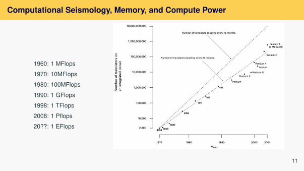
Computational Seismology, Memory, and Compute Power

1960: 1 MFlops

1970: 10MFlops

1980: 100MFlops

1990: 1 GFlops

1998: 1 TFlops

2008: 1 Pflops

20??: 1 EFlops

11

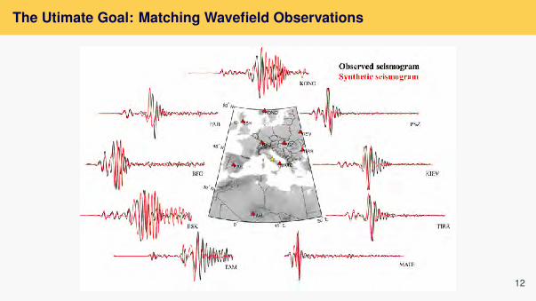
The Utimate Goal: Matching Wavefield Observations

12

A Bit of Wave Physics

Acoustic wave equation: no source

Acoustic wave equation

∂2t p = c2∆p + s

p → p(x, t), pressurec → c(x), velocitys → s(x, t), source term

Initial conditions

p(x, t = 0) = p0(x, t)

∂tp(x, t = 0) = 0Snapshot of p(x, t) (solid line) after some time forinitial condition p0(x, t) (Gaussian, dashed line),1D case.

13

Acoustic wave equation: external source

Green’s Function G

∂2t G(x, t ; x0, t0)− c2∆G(x, t ; x0, t0) = δ(x− x0)δ(t − t0)

Delta function δ

δ(x) =

{∞ x = 00 x 6= 0

∫ ∞−∞

δ(x)dx = 1 ,∫ ∞−∞

f (x)δ(x)dx = f (0) δ-generating function usingboxcars.

14

Acoustic wave equation: analytical solutions

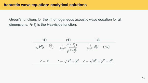
Green’s functions for the inhomogeneous acoustic wave equation for alldimensions. H(t) is the Heaviside function.

1D 2D 3D12c H(t − |r |

c ) 12πc2

H(t− |r|c )√t2− r2

c2

14πc2r δ(t − r/c)

r = x r =√

x2 + y2 r =√

x2 + y2 + z2

15

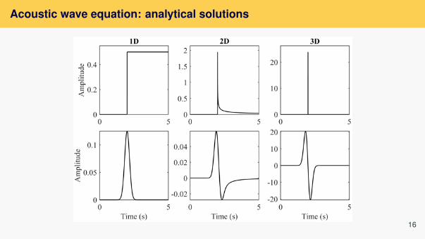
Acoustic wave equation: analytical solutions

16

Wave Equation as Linear System

• Accurate Green’s functions cannotbe calculated numerically

• A numerical solver is a linearsystem

• The convolution theorem applies

• Inaccurate simulations can be filteredafterwards

• Source time functions can be alteredafterwards

• ... provided the sampling is goodenough ...

17

Numerical Methods for WavePropagation Problems

Spatial Scales, Scattering, Solution Strategies

• Recorded seismograms are affectedby ...

• ... the ratio of seismic wavelength λand structural wavelength a ...

• ... how many wavelengths arepropagated ...

• strong scattering when a ≈ λ →numerical methods

• ray theory works when a >> λ

• random medium theory necessaryfor strong scattering media (and longdistances)

18

What’s on the market

• The finite-differencemethod

• The pseudospectal method

• The finite-element method

• The spectral-elementmethod

• The finite-volume method

• The discontinuous Galerkinmethod

19

The Finite-Difference Method

Finite differences in a Nutshell

• Direct numerical approximation of partialderivatives using finite-differences

• Local computational scheme→ efficientparallelisation

• Very efficient on regular grids, cumbersomefor strongly heterogeneous models

• Boundary conditions difficult to implementwith high-order accuracy

• The method of choice for models with flattopo and moderate velocity perturbations

• Highly efficient extensions possible, butrarely used!

20

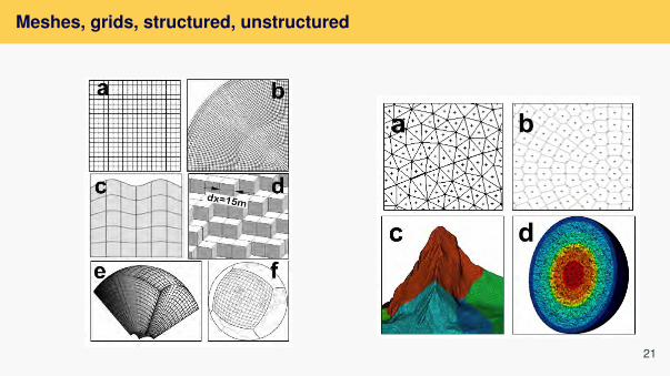
Meshes, grids, structured, unstructured

21

von Neumann Analysis, Stability, Dispersion

• Plane waves in a discreteworld

• p(x , t) = ek j dxx−wn dt

• Simulations are conditionallystable

• c dtdx ≤ ε ≈ 1 CFL - criterion

• Simulated phase velocitybecomes numericallydispersive!

• The more points perwavelength the more accurate

• How to check?

22

Numerical Anisotropy

23

Applications, recent , community codes

Source: geodynamics.org (SW4)

• Method of choice for flat surfaces andbody wave problems (exploration)

• Problems for strong topography

• Very accurate (optimal) operatorspossible, but ...

• Summation-by-parts approach(better for topography)

• Combination with homogenisation(regular grid revival)

• Community codes: SW4 (CIG),SOFI3D (Karlsruhe)

24

The Pseudospectral Method: theroad to spectral elements

The Pseudospectral Method in a Nutshell

• Calculation of exact derivatives inspectral domain

• Less dispersive than thefinite-difference method (isotropicerrors)

• Boundary conditions hard toimplement

• Global communication scheme→inefficient parallelisation

• Combinations with FD possible

• Hardly in use today, but conceptsused in the spectral-element method

25

Exact interpolation/derivative: Fourier Series

26

Applications, recent developments

Seismic wave simulation in the Moon (Wang et al., GJI, 2013)

• Axisymmetric wavepropagation (GroupProf. Furumura)

• Implementation inspherical coordinates

• Pseudospectralapproach in θ direction

• Finite-differenceapproach in radialdirection

• Used in combinationwith axisem (→axisem3d)

27

The Finite-Element Method

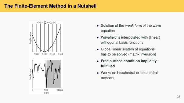
The Finite-Element Method in a Nutshell

• Solution of the weak form of the waveequation

• Wavefield is interpolated with (linear)orthogonal basis functions

• Global linear system of equationshas to be solved (matrix inversion)

• Free surface condition implicitlyfullfilled

• Works on hexahedral or tetrahedralmeshes

28

Linear basis functions, system matrices

Linear finite-element method and low-order finite-difference method are basically identical

29

Applications, Recent Developments

Finite element mesh, octree approach

(Bielak et al.)

• Requires linear algebra libraries formatrix inversion

• Suboptimal for parallelization

• Allows arbitrary geometric complexity

• Curbed element boundaries possible

• Standard in engineering applications

• Hardly used in seismology (why?)

30

The Spectral-Element Method

The Spectral-Element Method in a Nutshell

• Same mathematical derivation as thefinite-element method

• Lagrange polynomial representationof wave field

• Gauss-Lobatto-Legendre collocationpoints (stability!)

• Diagonal mass matrix→ triviallyinverted

• Explicit extrapolation scheme→efficient parallelisation

• Method of choice for global wavepropagation (specfem, axisem)

• Meshing required31

Lagrange polynomials, interpolation

• Uneven gridspacing forhigh-orderpolynomials→time-stepping

• Maximum orderusually N=4

• Chebyshev wasfirst (why?)

32

Numerical integration

• Galerkin methods necessitateintegral calculations overelements

• They are the only source oferrors in the spacediscretization (SE)

• Integration with Chebyshevpolynomials would be exactup to order N

• Integration with samecollocation points asinterpolation

33

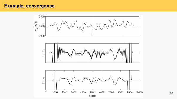
Example, convergence

34

Applications, Recent Developments

• Many applications in regional andglobal seismology

• Method of choice whenever surfacewaves are involved

• Spherical geometry with cubedsphere approach

• Applications to soil-structureinteraction

• Works for hexahedral and tetrahedralmeshes (→ salvus)

• specfem maybe most widely usedcommunity software for globalseismology (3D)

35

The Finite-Volume Method

The Finite-Volume Method in a Nutshell

• Mathematically derived as aconservation law

• Spatial discretization with arbitraryvolumes

• Extreme geometric flexibility (e.g.,shock waves)

• Voronoi cells, tetrahedra, polygons

• Entirely local formulation (cell based)

• Communication with neighboursthrough flux scheme

• Hardly used in seismology

36

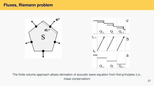
Fluxes, Riemann problem

The finite-volume approach allows derivation of acoustic wave equation from first principles (i.e.,mass conservation)

37

Applications, Recent Developments

Kaeser et al., 2000

• Method of choice for conservationproblems with strongly discontinuoussolutions

• Many applications in geophysicalfluid dynamics

• Relatively simple, finite-differencestyle algorithms

• Linear extrapolation schemesstrongly diffusive

• Recent general extensions to higherorder

• Potential for seismology not fullyexplored

38

The Discontinuous GalerkinMethod

The Discontinuous Galerkin Method in a Nutshell

• Numerical solution of first-ordersystems

• Developed for hyperbolic problems(e.g., neutron diffusion)

• Local formulation for each element

• Solution of weak form of waveequation

• Communication between elementsthrough fluxes→ FV

• Explicit time extrapolation→ efficientparallelisation

• Nodal and modal approaches forhexahedral and tetrahedral meshes 39

Fluxes, tetrahedral meshes

The first competitive scheme for tetrahedral meshes in seismology, but ...

40

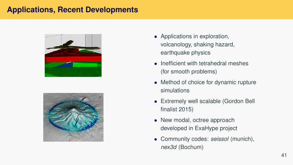
Applications, Recent Developments

• Applications in exploration,volcanology, shaking hazard,earthquake physics

• Inefficient with tetrahedral meshes(for smooth problems)

• Method of choice for dynamic rupturesimulations

• Extremely well scalable (Gordon Bellfinalist 2015)

• New modal, octree approachdeveloped in ExaHype project

• Community codes: seissol (munich),nex3d (Bochum)

41

"Meet the future ..."

42

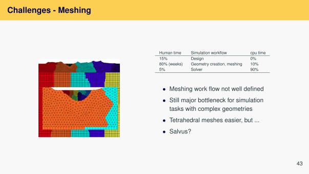
Challenges - Meshing

Human time Simulation workflow cpu time15% Design 0%80% (weeks) Geometry creation, meshing 10%5% Solver 90%

• Meshing work flow not well defined

• Still major bottleneck for simulationtasks with complex geometries

• Tetrahedral meshes easier, but ...

• Salvus?

43

Spectral element method - Salvus

• In development at ETH

• Spectral-elementimplementation

• tetrahedral and hexahedralmeshes

• built on top of communitylibraries (e.g., PetSc)

• Meshing routines for somemodel classes

44

Future Strategies - Alternative Formulations

Al-Attar and Crawford GJI 2016

• Particle relabelling

• Summation-by-parts

• Mapping geometricalcomplexity onto regular grids

• Smart pre-processing ratherthan meshing?

• Similar concept used insummation-by-parts (SBP)algorithms (SW4)

45

Future Strategies - Homogenization

• We only see low-passfiltered Earth

• So why simulate modelswith infinite frequencies?

• Homogenisation ofdiscontinuous model

• Renaissance of regulargrid methods?

46

Challenges - Community Platforms

www.verce.eu

• Science gateways for basicsimulation tasks

• High level model initialization

• Large scale simulations -hidden supercomputers

• Complex admission protocols

• Black boxes

• Great idea, but ...

47

Computational Seismology, Practical Exercises, Jupyter Notebooks

• Jupyter notebooks are interactivedocuments that work in any browser

• Simple text editing

• Inclusion of graphics

• Equations with Latex

• Executable code cells with Python (or else)

• The coolest thing since ...

• Many examples on: www.seismo-live.org

• Computational Seismology: A PracticalIntrodcution (Oxford University Press)

Try it out!

48

Conclusions

The forward problem is solved, but ...

49