Concentrated Ownership and Bailout Guarantees∗

Martin Schneider

NYU and FRB Minneapolis

Aaron Tornell

UCLA and NBER

November 2005

JEL Classification No. E20, E30, F40, O41

Abstract

This paper studies the effect of bailout guarantees in an economy where ownership of firms is con-

centrated. In contrast to standard models of deposit insurance, bailout guarantees need not generate

excessive risk taking, but may instead alleviate underinvestment. While the economy can experience

wasteful lending booms, such booms often end in a self-correcting soft landing, as in the data. However,

an economy that operates efficiently can also relapse into episodes of inefficient over- or underinvestment.

Financial development has unintended consequences as it provides markets with tools to better exploit

the bailout guarantee.

∗We would like to thank Pierre Gourinchas, Elhanan Helpman, Boyan Jovanovic, Anne Krueger, Lars Ljungqvist, Monika

Piazzesi, Thomas Sargent, Jeremy Stein and seminar participants at Berkeley, Brown, the Federal Reserve Banks of New York

and San Francico, Harvard, the IMF, MIT, Munich, NBER Monetary Economics Conference, Stanford, UCLA and the World

Bank. Some of the results of this paper were previously circulated under the title “Lending Booms and Asset Price Inflation".

The views herein are those of the authors and not necessarily those of the Federal Reserve Bank of Minneapolis or the Federal

Reserve System.

1. Introduction

A country experiencing a lending boom goes through a period of unusually fast growth in credit. Lending

booms occur frequently in emerging markets and are often accompanied by asset price inflation and strong

investment growth.1 In addition, many recent financial crises were preceded by lending booms. It is often

argued that lending booms are the result of mistaken government policy: the existence of bailout guarantees

creates a moral hazard problem that entails overborrowing, excessive investment and risk taking. A boom

then ends once it is realized that further guarantees are not credible and a crisis ensues.

The standard moral hazard account of lending booms suffers from two drawbacks. First, the typical boom

does not end in a crisis. Instead, many lending booms end in a soft landing, with credit and asset prices

gradually reverting to trend (Gourinchas et al. 2001). Second, the formal underpinnings of the standard

story derive from the deposit insurance literature, which was developed to study optimal financing and risk

taking by banks in developed countries. In particular, it assumes frictionless capital markets: leverage does

not affect the cost of capital. This assumption makes gambling with borrowed money particularly attractive.

However, it is implausible in the light of recent evidence on ownership structure.2 In emerging economies,

controlling shareholders often hold large stakes, even in large firms. This suggests that external finance is

costly, and therefore that incentives for inefficient risk taking may be much weaker.

This paper develops a theory of lending booms in economies where production is controlled by wealthy

entrepreneurs. We show that, in such economies, lending booms fuelled by guarantees can occur, but tend

to naturally end in a soft landing. In our model, entrepreneurs hold large stakes in their firms, because

contracts cannot be enforced perfectly. Bailout guarantees encourage overinvestment and risk taking, as

in existing models. However, the new theme is that entrepreneurs trade off any gains from exploiting a

guarantee (through risk-taking) against losses to their own capital. This tradeoff changes over time with the

level of entrepreneurial net worth, which gives rise to rich dynamics for investment and asset prices.

In equilibrium, our economy moves into and out of three distinct phases. At low levels of entrepreneurial

net worth, the high cost of external finance hampers investment. In this phase of inefficient under investment,

bailout guarantees actually foster growth since they provide a substitute for scarce capital. The moral hazard

problem emerges only at intermediate levels of net worth, where it leads to inefficient over investment. A

third phase occurs when net worth is high enough relative to existing investment opportunities. Once

entrepreneurs have a sufficient amount of capital at stake, they forego inefficient and highly risky projects

and investment is efficient.

A lending boom that ends in a soft landing is a transition path that passes through all three phases.

At the beginning of the boom, entrepreneurs have little capital. While firms are highly leveraged and the

1A set of references on these stylized facts is provided below.2Bekaert and Harvey (2003) survey studies that provide evidence on capital market imperfections in emerging economies.

2

conditional volatility if output is high, expected returns are also high. A sequence of favorable productivity

shocks then increases profits and hence internal funds, thus fueling investment until the boom evetually

“overheats”. In particular, although entrepreneurs may have sufficient internal funds that they could invest

efficiently, guarantees encourage them to leverage up their firms further and invest in low-return projects.

The economy thus enters a phase of high risk and low expected returns. However, unless an exogenous

shock triggers a crisis during this phase, entrepreneurs eventually grow out of it: as their net worth increases

further, leveraged strategies become too risky and investment is cut back to produce a soft landing.

The model also helps understand the behavior of asset prices during lending booms. The prices of

productive assets often rise in booms to levels that are hard to reconcile with historical fundamentals. In

our model, this happens because asset prices capitalize future subsidies implicit in bailout guarantees. The

effect is reinforced if the country recently experienced an improvement in contract enforcement which makes

it easier to exploit guarantees. In addition, returns in the beginning of a boom tend to be volatile and

negatively skewed. In our model, this feature arises naturally from the asymmetric adjustment costs implied

by financing constraints. Finally, asset prices in our model typically peak well before the lending boom ends:

they anticipate the soft landing.

Economic downturns in our model occur for two reasons. First, there might simply be a sequence of bad

shocks. For example, a sequence of unfavorable terms-of-trade movements lowers profits and hence entre-

preneurial net worth and could move the economy into the underinvestment region. In addition, transitions

to the underinvestment phase can occur endogenously. Indeed, the nonlinear dependence of investment on

entrepreneurial net worth implies that the economy can exhibit endogenous cycles even if productivity is

constant. While overheating booms generate profits that trigger a soft landing, profits after the soft landing

decline and may cause a relapse into the overinvestment phase. The interaction of bailout guarantees and

credit market frictions is thus by itself a source of volatility.

In our model economy, financing constraints bind even though bailout guarantees are present. This is

not a foregone conclusion: if a bailout always occurs in case of default, why should lenders care whether

borrowers can commit to repay? The reason is that bailout guarantees insure lenders only against systemic

risk. A bailout does not occur if just an isolated firm defaults, especially not a small one. Instead, bailouts

happen only when there is a critical mass of defaults. Collateral then still matters for credit, because lenders

have to guard against idiosyncratic default risk.

Exploiting a systemic guarantee requires that entrepreneurs coordinate on risky strategies that lead

to widespread default. This coordination problem is another source of fluctuations. Indeed, the risky

overinvestment strategies that drive an overheating lending boom are optimal for an individual entrepreneur

only if he expects others to engage in similar activities, so that default actually triggers a systemic bailout.

As a result, a lending boom may end in a “correction”, where entrepreneurs revert to efficient investment

3

because they no longer trust others to continue similar risky strategies. More generally, mutual trust among

entrepreneurs becomes a second source of (exogenous) shocks in our model.

A key feature of our model is that entrepreneurs and lenders implicitly collude to exploit the bailout

guarantee. This has immediate implications for policy. While better enforceability of contracts may avoid

inefficient underinvestment early on during a lending boom, it also fosters more inefficient overinvestment

as the lending boom overheats. The reason is that a better contracting technology provides entrepreneurs

and lenders with a more effective tool to exploit the guarantee. This contradicts conventional wisdom that

better contract enforcement should improve the allocation of resources. It follows that institutional changes

that improve contract enforcement may not be desirable unless at the same time a regulatory framework is

put in place that contains excessive risk taking.

The literature on moral hazard due to bailout guarantees is large. Roubini and Setser (2004) provide an

overview of recent work that applies this concept to emerging economies.3 In terms of formal dynamic analy-

sis, Krugman (1998), Corsetti et al. (1999), Ljungqvist (2002) and Eichenbaum et al. (2004) have studied

moral hazard in the context of a neoclassical growth model with frictionless credit markets. Borrowers are

then competitive firms and shareholder wealth does not matter for investment. The key mechanism gener-

ating soft landings in our model is thus absent. More generally, our new results derive from the interaction

of bailout guarantees with lack of contract enforceability that we view as an important institutional feature

of emerging economies.

Our model is also related to financial accelerator models of the business cycle. Following Bernanke and

Gertler (1989), a number of authors have explored the macroeconomic implications of credit market frictions.4

However, we show that the presence of bailout guarantees overturns several results typically associated with

financial accelerator models. First, our model gives rise to both over- and underinvestment, whereas typically

financing constraints induce only underinvestment. As a result, better contract enforcement or infusions of

net worth do not necessarily improve efficiency of investment in our model. Second, because of the soft

landing effect, a positive shock to net worth may decrease investment in our model. This means that the link

between cash flow and investment is nonlinear: it is positive for firms with low net worth, but negative when

net worth is higher. Simple linear regression analysis of the relationship between cash flow and investment

may thus not be able to uncover the importance of financing constraints.

The paper proceeds as follows. The remainder of this introduction briefly points to evidence on lending

booms and the distortions we focus on. Section 2 presents our model of a entrepreneurial firms in a small

3See Freixas and Rochet (1998) for an exposition of the theory of deposit insurance.4These papers embed frictions that are familiar from standard static models of the debt constrained entrepreneurial firm

into a macro framework. For example, moral hazard with costly state verification (Townsend (1979), is employed in Bernanke

and Gertler (1989,1998) and Carlstrom and Fuerst (1996); ex ante moral hazard, studied by Holmstrom and Tirole (1995), is

used by Aghion and Bolton (1995); Kiyotaki and Moore (1997) rely on a version of the Hart and Moore (1994,1997) incomplete

contracting theory of debt finance.

4

open economy. Section 3 derives optimal leverage policy when bailout guarantees are present. Section 4

derives proporties of the business cycle and asset prices. Some proofs are collected in an appendix.

Empirical Evidence on Lending Booms and Distortions

The existing evidence on lending booms can be read as answering two questions. The first question is what

are the salient features of macroeconomic aggregates and relative prices during an episode. During a typical

boom, investment and asset prices rises along with credit. For example, Pomerleano (1998) considers data

from 734 South East Asian corporations from 1992 to 1996. For the case of Thailand, the average investment

rate during this period was 29% (3% in the US). Furthermore, 78% of this investment was financed with

debt (8% in the US). Claessens et.al. (1999), using a database of 5550 firms in nine Asian countries, find

that during the early 1990s investment and leverage were very high and increasing. In Thailand during

1988-95 the investment rate increased from 10% to 14.5%, the debt-to-equity ratio increased from 1.6 to

2.2. The corresponding figures for the US are 3.8 to 3.7 and 0.8 to 1.1. Guerra (1998) and Hernandez and

Landerretche (1998) document the appreciation of real estate and stock prices.

On average, lending booms do not end in a financial crisis, but rather in a “soft landing”. Asset prices

tend to revert before the lending boom ends. For example, Gourinchas et. al. (2001) find that in a sample

of 91 countries over the past 35 years, the probability that a lending boom will end in a currency crisis is

less than 20%. Furthermore, the build-up and ending phases of an average boom are similar in magnitude

and duration. Although abrupt collapses of booms are not the norm, it is true that almost all banking and

currency crises in emerging markets have been preceded by lending booms (see, for example, Corsetti et al.

1998, Kaminsky and Reinhart 1999 and Tornell 1999). Moreover, those lending booms that have ended in a

crisis have typically been followed by a credit crunch. That is, in the aftermath of crises new lending falls

sharply and recuperates only gradually (Krueger and Tornell 1999; Sachs et al. 1995).

A second empirical question is whether the quality and composition of investment is different during

lending booms, when compared to normal times. Naturally, an answer to this question is not as easily

quantifiable, and the existing evidence is largely anecdotal. Nevertheless, there does seem to be a tendency

for the quality of investment to deteriorate during lending booms. Pomerleano (1998) finds that the return

on assets in his sample of Thai firms fell from 9% in 1992 to 5% in 1996 (9% and 13% in the US). Claessens,

et.al. (1999) document that the real return on assets fell from 11% to 8%. Moreover, firms and banks have

been noted to shift to activities that have traditionally been considered to be more risky, such as investment

in real estate (BIS, 1999). Not all firms experience booms and busts in the same way. Small, bank-dependent

firms and firms in the nontradable sector have grown more strongly during the boom, but have been slower

to recover after the crisis than large exporting firms with access to direct finance (Krueger and Tornell 1999).

There is also some direct evidence that the two distortions we focus on are present especially in emerging

markets. On the one hand, bailout guarantees are present in many countries, and they tend not to be

5

accompanied by a strong regulatory framework (Roubini and Setser, 2004). On the other hand, claims on

firm insiders are not as easily enforceable as in developed countries, as external corporate governance tends

to be weak (Johnson et al. 2000, Klapper and Love 2002). The role of concentrated ownership in emerging

markets as a response to this has been emphasized by Himmelberg et al. (2002). The results of Harvey et al.

(2004) suggest that debt is used in part to alleviate the agency problems between controlling and minority

shareholders.

2. The Model

We consider a small open economy, populated by overlapping generations of risk neutral entrepreneurs.

The riskless world interest rate is fixed at r. Every entrepreneur in generation t owns a risky production

technology, which turns kt units of the single numeraire good invested in period t into

yt+1 = zt+1f (kt)

units of the good in period t+1. The productivity shock zt+1 is i.i.d. over time and equals one with probability

α, and zero otherwise. In addition, it is perfectly correlated across entrepreneurs. The production function

f is continuous, increasing and concave, with f (0) = 0 and limk→0 f 0 (k) =∞.An entrepreneur of generation t begins period t with internal funds wt. He can raise additional funds

bt by issuing one period bonds with a promised interest rate ρt to risk neutral foreign investors. Foreigners

have ‘deep pockets’: they are willing to lend any amount, provided that they expect to earn at least the

world interest rate. Entrepreneurs also have access to alternative investment opportunities that earn the

riskless rate, which we refer to as riskless savings st. The budget constraint is thus

st + kt = wt + bt. (2.1)

Distortions

The economy is subject to two distortions. First, entrepreneurs cannot commit to repay debt. In

particular, entrepreneurs of generation t may default strategically at date t + 1. Once they do so, lenders

seize entrepreneurs’ assets. However, the physical assets cannot be fully recovered: if kt was invested in

capital, lenders obtain only ψzt+1kt, where ψ ≤ 1 + r. The payoff to an entrepreneur who defaults is thus

Πdt+1 (zt+1) = zt+1(f (kt)− ψkt). (2.2)

The second distortion is the existence of bailout guarantees. We assume that an aid agency steps in

whenever more than half of all entrepreneurs default. The agency then takes over recovery of the delinquent

loans, and it pays lenders (1 + r)bt for every bt dollars lent. We do not address where the agency obtains

funds for a bailout, but treat the bailout as a windfall to the domestic entrepreneurial sector. One can

6

imagine either foreign aid or the domestic government levying taxes on the (unmodelled) household sector,

for example.

In the absence of strategic default, profits realized by generation t in t+ 1 are

Πt+1 (zt+1) = zt+1f (kt) + (1 + r) st − (1 + ρt) bt. (2.3)

Every “old” entrepreneur in t + 1 consumes cΠt+1. He then passes on the firm to his heir, a member of

generation t+1. This “young” entrepreneur thus starts operations with internal funds wt+1 = (1− c)Πt+1.

In contrast, if the firm is in default in t+1, the young entrepreneur starts over with wt+1 = ε.5 Throughout,

we take ε to be a number close to zero.

Equilibrium

The timing of events for a given generation of entrepreneurs and lenders is as follows. At date t, every

entrepreneur announces plans for risky investment kit and savings sit and debt b

it that satisfy 2.1, as well as

a promised interest rate ρit. Lenders then decide whether to accept or reject these offers. At date t+ 1, the

shock zt+1 is realized and entrepreneurs decide whether or not to default. A bailout occurs if more than

half of the entrepreneurs default. Since the bailout depends on the action of all entrepreneurs, individual

entrepreneurs’ payoffs are interdependent. Formally, the above description of actions and payoffs defines a

“credit market game” played by successive generations of entrepreneurs and lenders. Since all entrepreneurs

are identical and the shocks are perfectly correlated, it is natural to focus on symmetric equilibria of this

game.

We thus define an equilibrium of the model as a stochastic process (kt, st, bt, ρt, wt), such that (i) given

entrepreneurial wealth wt, there is a symmmetric subgame perfect equilibrium of the credit market game

in which entrepreneurs of generation t offer (kt, st, bt, ρt) and this offer is accepted by lenders of generation

t, and (ii) the wealth process evolves as follows: wt+1 = ε in states where the credit market equilibrium

played by generation t calls for default, and wt+1 = (1− c)Πt+1 otherwise, where entreprenuers’ profit Πt+1

is defined by (2.3).

Discussion

A. Discussion of setup section. Here we can adress:

1. nature of guarantees.

2. restrictions on parameters (c<1- , <...these now come late w/ propositions).

3. what is now section 3.1 defining k* and k** (now 3.1 looks like a detour; then sec 3.2 starts

repeating some material of 1st paragraph in sec3). We could then convert sec3.2 into opening part of sec3.

5An alternative and perhaps more natural assumption would be that every young entrepreneur receives an endowment ε,

together with a share of profits (1− δ)Πt+1. This would not significantly change the nature of the dynamics, but would make

the algebra significantly less transparent. We adopt the present assumption for simplicity.

7

4. we can interpret high c as a ‘high tax rate’ so we can link high-c case that converges to w<w* to

economies with voracious governments (and are thus in a low-growth trap with many crises, like in africa)

3. Credit Market Equilibrium

We characterize equilibria of the model in two steps. In this section, we discuss the interaction of a given

generation t of entrepreneurs with its lenders — the equilibrium of the date t credit market game. This

interaction determines what happens in the credit market at date t, and also whether a bailout occurs at

date t+1. The second step of the analysis will consider dynamics, where a sequence of credit market games

is connected by the passing down of firms and internal funds.

3.1. Frictionless benchmark

As a benchmark, it is helpful to consider what happens when firms have no capital at stake and face no

commitment problem, that is, if wt = 0 and ψ = 1 + r. This special case replicates familiar results from

competitive models in the literature. Suppose first that no bailout is expected. It is then optimal to invest

in physical capital to the point k∗ where the expected marginal product of capital is equal to the expected

rate of return that lenders must earn:

αf 0 (k∗) = 1 + r.

Since investment must be financed by borrowing, the firm will be forced into default in the bad state

(zt+1 = 0). The firm’s debt is thus risky. In fact, it does not pay for entrepreneurs to save at all (st = 0),

so that lenders do not receive any payoff in the bad state. To nevertheless ensure that lenders finance the

investment, entrepreneurs must pay an interest rate ρt =1+rα − 1 > r.

Now suppose instead that a bailout occurs in the bad state. Lenders know that the aid agency will pay

them (1 + r) per dollar lent in that state. As a result, entrepreneurs can borrow at the rate ρt = r that does

not provide compensation for default risk. While it is still not optimal to save, investment is now optimally

driven up to the point k∗∗ where the marginal product of capital conditional on the good state equals the

riskless rate:

f 0 (k∗∗) = 1 + r.

This is because the firm itself pays the interest rate only in the good state — the aid agency picks up the

tab in the bad state. We have k∗∗ > k∗, so that bailout guarantees increase investment. However, the extra

investment k∗∗− k∗ is channelled to “white elephant” projects that have ex ante negative net present value.

In the frictionless special cases presented so far, our model replicates the investment levels and interest

rates that occur in a standard model, used, for example, in the deposit insurance literature. However, we

emphasize that our model differs from that literature in what is exogenous to the firm in a given period.

8

Models of deposit insurance typically consider banks of fixed scale, but with variable capital chosen by

shareholders with “deep pockets”. The models then predict changes in leverage and risk as a result of changes

in regulation. For example, if capital requirements are relaxed, shareholders prefer higher leverage and

riskier loan portfolios. This setup is motivated by large US banks. In contrast, in our world of concentrated

ownership, firms have variable scale, but their capital is predetermined by the wealth of the entrepreneur.

Our model thus predicts changes in leverage and risk as a result of changes in past profits. This will also be

important below in our dynamic analysis.

3.2. Internal funds and strategic default risk

We now ask how the above results change if entrepreneurs (i) have limited access to external funds (ψ < 1 + r),

but (ii) do have access to internal funds (wt > 0). We focus on symmetric equilibria of the credit market

game, where all entrepreneurs choose the same strategies. Two types of equilibria of the credit market game

are of interest. In a risky equilibrium, investment is financed at least in part by borrowing and firms default

in the bad state. In contrast, in a safe equilibrium, investment is fully financed internally and there is no

default. The following proposition provides necessary and sufficient conditions for both types of equilibria

to exist. In particular, it relates the type of equilibrium to the level of entrepreneurial wealth.

Proposition 3.1. (Credit Market Equilibria)

1. There is a threshold level of internal funds w̃ ∈ (k∗, k∗∗) such that a risky equilibrium exists if and onlyif w ≤ w̃. In this equilibrium, entrepreneurs do not save and pay the rate ρt = r on their debt. Investment

is given by

k = min

½w

1− βψ, k∗∗

¾,

where β = 11+r . All entrepreneurs default if zt+1 = 0, and a bailout occurs in that state.

2. A safe equilibrium exists if and only if w ≥ k∗. In this equilibrium, entrepreneurs invest k = k∗ and

save s = w − k∗. They do not borrow.

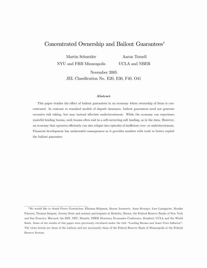
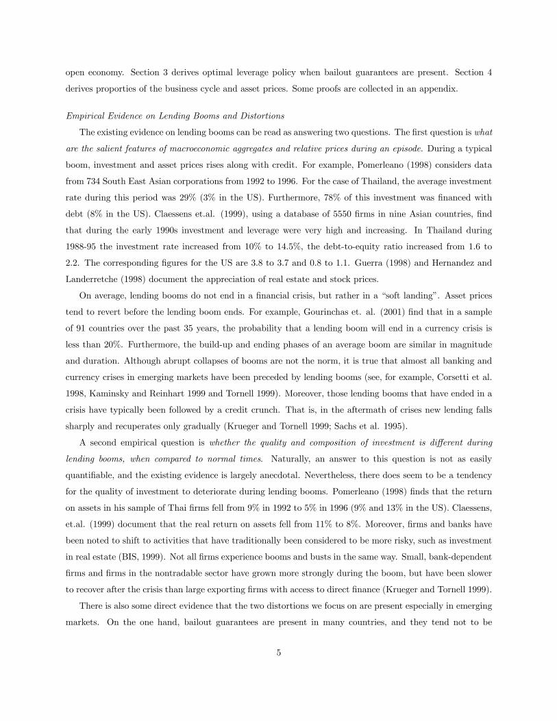
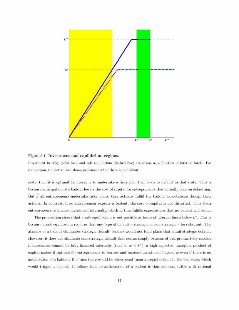
A proof of the proposition is contained in Subsection 3.3 below. We first represent graphically when

the different equilibria can occur. Figure 3.1 shows optimal investment in both safe (dashed line) and risky

(solid line) equilibria as a function of internal funds. Depending on the level of interval funds, the economy

can be in one of four regions: an underinvestment region, an overinvestment region, a region with multiple

equilibria and an efficient region. We now discuss all four regions in turn.

Underinvestment

For low internal funds (the area shaded in light gray that satisfies w < k∗ (1− βψ)), the unique equilib-

rium is risky, and all firms invest less than the first best level k∗. This underinvestment region arises because

9

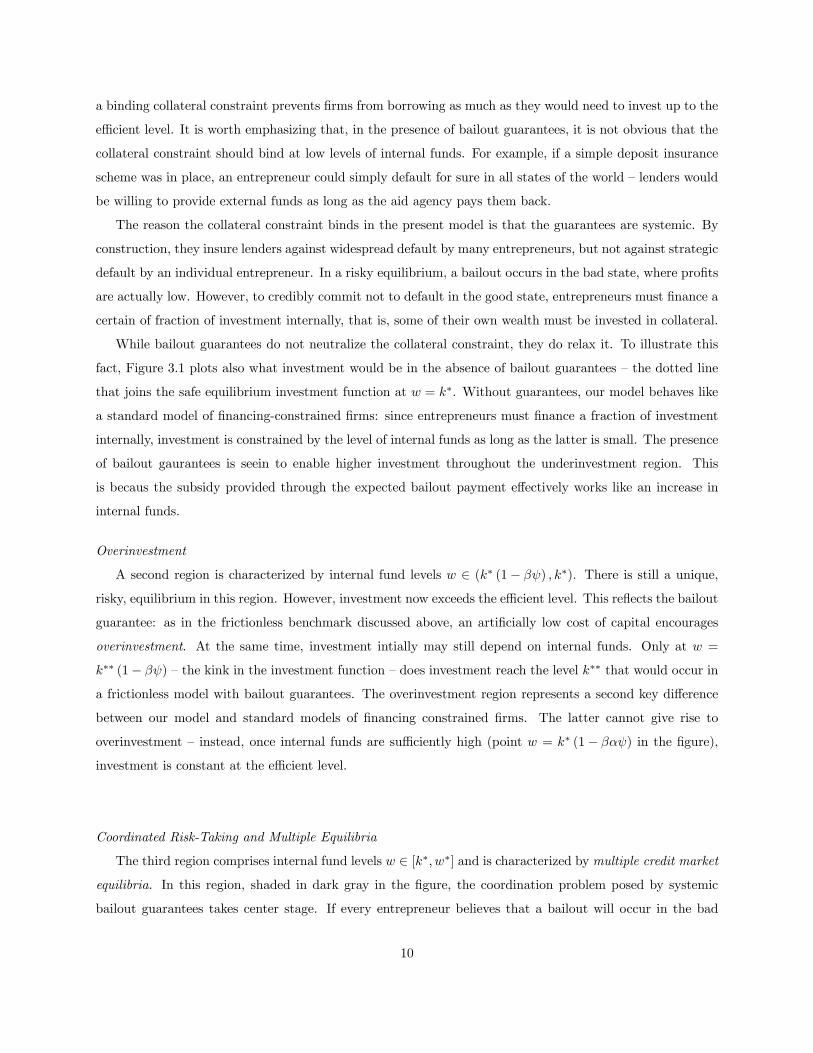
a binding collateral constraint prevents firms from borrowing as much as they would need to invest up to the

efficient level. It is worth emphasizing that, in the presence of bailout guarantees, it is not obvious that the

collateral constraint should bind at low levels of internal funds. For example, if a simple deposit insurance

scheme was in place, an entrepreneur could simply default for sure in all states of the world — lenders would

be willing to provide external funds as long as the aid agency pays them back.

The reason the collateral constraint binds in the present model is that the guarantees are systemic. By

construction, they insure lenders against widespread default by many entrepreneurs, but not against strategic

default by an individual entrepreneur. In a risky equilibrium, a bailout occurs in the bad state, where profits

are actually low. However, to credibly commit not to default in the good state, entrepreneurs must finance a

certain of fraction of investment internally, that is, some of their own wealth must be invested in collateral.

While bailout guarantees do not neutralize the collateral constraint, they do relax it. To illustrate this

fact, Figure 3.1 plots also what investment would be in the absence of bailout guarantees — the dotted line

that joins the safe equilibrium investment function at w = k∗. Without guarantees, our model behaves like

a standard model of financing-constrained firms: since entrepreneurs must finance a fraction of investment

internally, investment is constrained by the level of internal funds as long as the latter is small. The presence

of bailout gaurantees is seein to enable higher investment throughout the underinvestment region. This

is becaus the subsidy provided through the expected bailout payment effectively works like an increase in

internal funds.

Overinvestment

A second region is characterized by internal fund levels w ∈ (k∗ (1− βψ) , k∗). There is still a unique,

risky, equilibrium in this region. However, investment now exceeds the efficient level. This reflects the bailout

guarantee: as in the frictionless benchmark discussed above, an artificially low cost of capital encourages

overinvestment. At the same time, investment intially may still depend on internal funds. Only at w =

k∗∗ (1− βψ) — the kink in the investment function — does investment reach the level k∗∗ that would occur in

a frictionless model with bailout guarantees. The overinvestment region represents a second key difference

between our model and standard models of financing constrained firms. The latter cannot give rise to

overinvestment — instead, once internal funds are sufficiently high (point w = k∗ (1− βαψ) in the figure),

investment is constant at the efficient level.

Coordinated Risk-Taking and Multiple Equilibria

The third region comprises internal fund levels w ∈ [k∗, w∗] and is characterized by multiple credit marketequilibria. In this region, shaded in dark gray in the figure, the coordination problem posed by systemic

bailout guarantees takes center stage. If every entrepreneur believes that a bailout will occur in the bad

10

0 k* w* k**

k*

k**

Figure 3.1: Investment and equilibrium regions.

Investment in risky (solid line) and safe equilibrium (dashed line) are shwon as a function of internal funds. For

comparison, the dotted line shows nvestment when there is no bailout.

state, then it is optimal for everyone to undertake a risky plan that leads to default in that state. This is

because anticipation of a bailout lowers the cost of capital for entrepreneurs that actually plan on defaulting.

But if all entrepreneurs undertake risky plans, they actually fulfill the bailout expectations though their

actions. In contrast, if no entrepreneur expects a bailout, the cost of capital is not distorted. This leads

entrepreneurs to finance investment internally, which in turn fulfills expectations that no bailout will occur.

The proposition shows that a safe equilibrium is not possible at levels of internal funds below k∗. This is

because a safe equilibrium requires that any type of default — strategic or non-strategic — be ruled out. The

absence of a bailout eliminates strategic default: lenders would not fund plans that entail strategic default.

However, it does not eliminate non-strategic default that occurs simply because of bad productivity shocks.

If investment cannot be fully financed internally (that is, w < k∗), a high expected marginal product of

capital makes it optimal for entrepreneurs to borrow and increase investment beyond w even if there is no

anticipation of a bailout. But then there would be widespread (nonstrategic) default in the bad state, which

would trigger a bailout. It follows that no anticipation of a bailout is thus not compatible with rational

11

expectations at low levels of internal funds.

Full Internal Finance

The fourth and final region consist of internal funds levels w > w∗. In this region, there is a unique

safe equilibrium where all investment is financed internally. The previous paragraph explains why a safe

equilibrium can occur when internal funds are high enough. The important feature of the fourth region is

that a risky equilibrium cannot occur. The reason is concentrated ownership. For rich entrepreneurs, the

expected benefit from the bailout guarantee does not outweigh the loss of own capital in the event of a

default. Unfair bets only pay off when they can be financed with money borrowed at subsidized rates. Rich

entrepreneurs will therefore forego overinvestment and excessive risk taking even when a bailout is expected.

Instead, they prefer to invest at the efficient level k∗, which they can finance internally. But this implies

that no bailout can be expected in equilibrium, since no defaults will take place.

3.3. Proof of Proposition 3.1

This section provides a proof of Proposition 3.1 that focuses on the economic intuition, with technical details

relegated to the appendix. The reader mostly interested in macroeconomics may wish to skip this subsection

proceed directly to the dynamic analysis in Section 4. In what follows, we refer to plans that involve no

savings and lead to default in the bad state, but not in the good state, as risky plans. We also call plans

that involve no borrowing safe plans. The appendix shows that only these two types of plans can ever occur

in equilibrium. To prove part 1 of the proposition, we now establish that, if a bailout is expected in the bad

state only, then it is optimal for a firm to offer a risky plan if and only if w < w∗. If all firms adopt a risky

plan, a bailout indeed occurs in the bad state, and a risky equilibrium is shown to exist.

The Role of Distortions: Subsidy and Collateral Constraint

Suppose a bailout is expected in the bad state only. The guarantee implies that lenders are happy to

accept the riskless rate ρt = r on risky plans. Using this value for the interest rate as well as the budget

constraint (2.1) and the definition of profits (2.2), entrepreneurs’ expected payoff can be written as

V (kt, wt) = (1 + r)wt + [αf (kt)− (1 + r) kt] + (1− α) (1 + r)max {kt − wt, 0} (3.1)

Here the second term represents profits from physical investment, while the third term captures the subsidy

due to the bailout guarantee. The latter can be claimed by picking a risky plan (which implies kt ≥ wt), but

is foregone when picking a safe plan (kt ≤ wt) .

The objective (3.1) is maximized subject to the constraint that there be no default in the good state,

(1 + ρt) bt ≤ ψkt + (1 + r) st. (3.2)

12

This condition is a collateral constrant — the entrepreneur can pledge all his savings, but only a limited

amount of the funds invested in physical capital. Using again the budget constraint to substitute, we obtain

the equivalent formulation

(1− βψ) kt ≤ wt.

Since capital cannot be fully pledged, at least a share 1− βψ of any investment in capital must be financed

internally.

Optimal Safe and Risky Plans

It is now straightforward to calculate the best risky and the best safe plan. If the entrepreneur opts

for a safe plan, he will try to operate the technology at the first best level k∗. In case internal funds are

insufficient to finance k∗, the marginal product is higher than 1+r and all internal funds should be invested.

The optimal safe investment is thus ks (wt) := min {wt, k∗}. In contrast, under a risky plan, the subsidy

provided through the bailout is increasing in the amount borrowed. As under the competitive benchmark,

this artificially lowers the marginal cost of capital and the entrepreneur would like to invest up to k∗∗.

Again, this desired amount can only be financed if sufficient internal funds are available, since the collateral

constraint still limits firm leverage. As long as wt ≤ k∗∗, the optimal risky investment is thus

kr (wt) =

wt1−βψk if wt < (1− βψ) k∗∗

k∗∗ if (1− βψ) k∗∗ < wt ≤ k∗∗

For wt > k∗∗, there does not exist an optimal risky plan — the safe plan that sets kt = wt dominates all risky

plans, and the entrepreneur would like to be as close as possible to that safe plan.

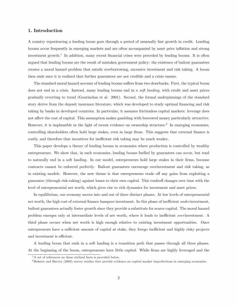
Trading off Subsidy versus Efficiency

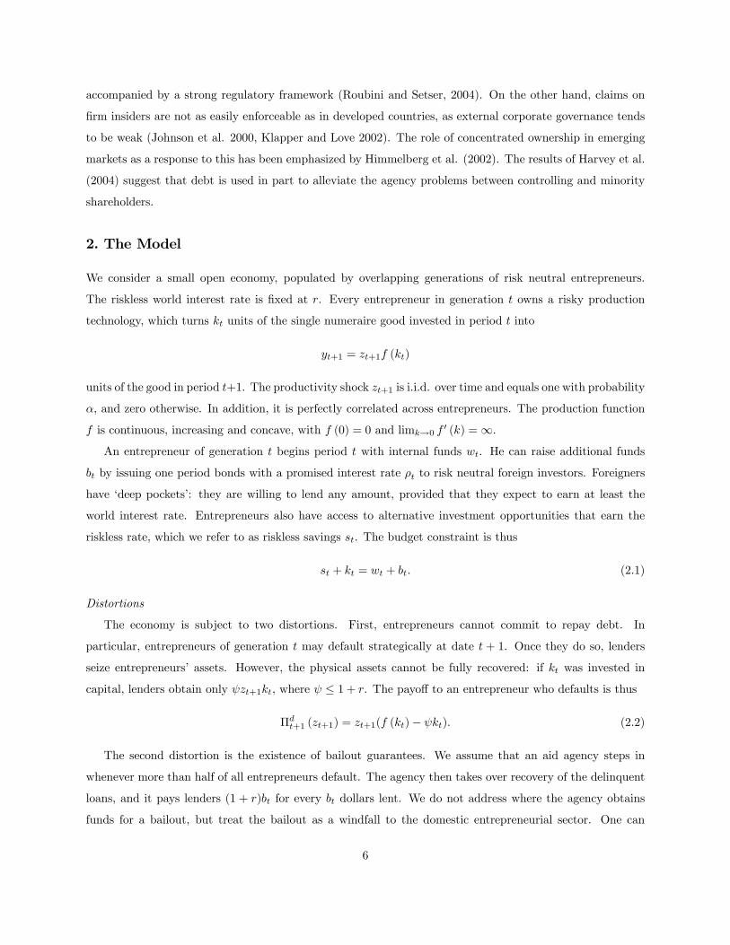
It remains to compare profits under the best risky and safe plan, V (kr (w) , w) and V (ks (w) , w) , re-

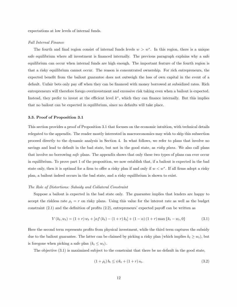
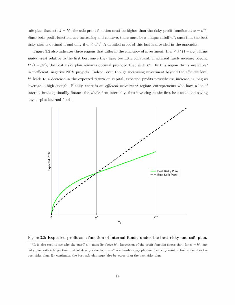
spectively, to determine the overall optimal plan. Figure 3.2 plots both profit functions and shows that the

best risky plan is optimal for low internal funds, while the best safe plan in optimal for high internal funds.

To understand this result, consider first the slope of both profit functions at w = 0. Since we have assumed

f 0 (0) > 1 + r, we have

∂

∂wV (kr (w) , w)

¯̄̄̄w=0

=1

1− βψ(αf 0 (0)− ψ) > αf 0 (0) =

∂

∂wV (ks (w) , w)

¯̄̄̄w=0

.

Under a risky plan with maximum leverage, a dollar of internal funds permits (1− βψ)−1 dollars of invest-

ment. Even though a share ψ of this investment (in future value terms) must be be pledged to lenders, the

high marginal product makes the risky plan overall more profitable than a safe plan that permits only one

dollar of investment per dollar of internal funds.

Consider now consider a high level of internal funds. We have already argued above that, for w > k∗∗,

any risky plan is dominated by the safe plan that sets k = w. Since the latter plan is worse than the best

13

safe plan that sets k = k∗, the safe profit function must be higher than the risky profit function at w = k∗∗.

Since both profit functions are increasing and concave, there must be a unique cutoff w∗, such that the best

risky plan is optimal if and only if w ≤ w∗.6 A detailed proof of this fact is provided in the appendix.

Figure 3.2 also indicates three regions that differ in the efficiency of investment. If w ≤ k∗ (1− βψ) , firms

underinvest relative to the first best since they have too little collateral. If internal funds increase beyond

k∗ (1− βψ), the best risky plan remains optimal provided that w ≤ k∗. In this region, firms overinvest

in inefficient, negative NPV projects. Indeed, even though increasing investment beyond the efficient level

k∗ leads to a decrease in the expected return on capital, expected profits nevertheless increase as long as

leverage is high enough. Finally, there is an efficient investment region: entrepreneurs who have a lot of

internal funds optimallly finance the whole firm internally, thus investing at the first best scale and saving

any surplus internal funds.

0 w* k**w

t

Expe

cted

Pro

fit

Best Risky PlanBest Safe Plan

Figure 3.2: Expected profit as a function of internal funds, under the best risky and safe plan.6 It is also easy to see why the cutoff w∗ must lie above k∗. Inspection of the profit function shows that, for w = k∗, any

risky plan with k larger than, but arbitrarily close to, w = k∗ is a feasible risky plan and hence by construction worse than the

best risky plan. By continuity, the best safe plan must also be worse than the best risky plan.

14

Safe Equilibria

We now assume that there is no bailout, and show that the optimal plan is safe if and only if w ≥ k∗.

Since there is indeed no bailout if everyone adopts a safe plan, this establishes existence of a safe equilibrium

(part 2 of the proposition). In the absence of bailouts, lenders will only fund a risky plan if they are paid

the interest ρt =1+rα − 1 that compensates them for default in the bad state. As a result, the entrepreneur’s

expected profit no longer includes the expected benefit from the guarantee and reduces to

V (kt, wt) = (1 + r)wt + [αf (kt)− (1 + r) kt] . (3.3)

In addition, the collateral constraint becomes more stringent: substituting into (3.2) and using the new

interest rate delivers

(1− αβψ) kt ≤ wt.

Since capital is lost in the bad state, the entrepreneur can effectively only pledge a share αβψ and must

come up with (1− α)βψ of additional internal funds. This is less than in the bailout case, where the aid

agency effectively insured the pledged capital in the bad state.

This formulation leads directly to the optimal plan: investment is

min

½wt

1− αβψ, k∗¾.

Clearly, the optimal plan is safe if and only if wt ≥ k∗. At any lower level of internal funds, investment is

partly financed by borrowing, so that the firm must default in the bad state.

4. Dynamics

To characterize equilibrium dynamics, it is convenient to introduce some additional notation. Every equilib-

rium of the model implies a sequence of equilibria of the credit market game. Let ηt ∈ {r, s} indicate whethera risky or a safe equilibrium is played in period t. In those periods in which wt lies in the multiple equilibria

region [k∗, w∗], we need a selection rule. We assume that there is a stochastic process xt, valued in {r, s}that determines which credit market equilibrium is played. This process represents entrepreneurs’ mutual

trust in each others’ willingness to take risk and hence trigger a bailout in the bad state. The sequence η

can then be expressed as a function of internal funds and the mutual trust variable x:

ηt = η (wt, xt) =

r if wt < k∗

s if wt > w∗

xt if wt ∈ [k∗, w∗]

Using the results from Proposition 3.1, an equilibrium process of internal funds {wt} is a solution to the

15

stochastic difference equation

wt+1 =

(1− c) zt+1

³f³min

nwt

1−βψ , k∗∗o´+ (1 + r)

³wt −min

nwt

1−βψ , k∗∗o´´

+(1− zt+1) εif ηt (wt, xt) = r

(1− c) (zt+1f (k∗) + (1 + r) (wt − k∗)) if ηt (wt, xt) = s

(4.1)

The current level of internal funds — and possibly mutual trust x — determine investment and borrowing in

t. The productivity shock zt+1 then determines internal funds in t + 1. If a safe equilibrium was played,

the economy has a “cushion” wt − k∗ to fall back on — a bad productivity shock will not lead to defaults.

In contrast, a risky equilibrium entails widespread default when zt+1 = 0 and the economy will restart at

wt = ε.

Consider now an economy that starts at the state wt = ε. As long as productivity is high (zt = 1) and

trust is strong (xt = r), the economy will follow a path of high investment and high entrepreneurial profits.

We refer to this path as the lucky path. An economy on the lucky path can experience four types of notable

events. On the one hand, either one of the exogenous shocks may throw the economy off the lucky path.

We call a period of unusually low productivity (zt = 0) a crisis. In a crisis, both ex ante good and ex ante

excessive (negative NPV) projects fail and output is zero. In contrast, a correction is a drop in investment,

brought about by a breakdown in mutual trust (xt = s). A correction does not affect productivity and

current output, although it does affect output with a lag through its effect on investment.

On the other hand, we emphasize two events that occur along the lucky path and are not triggered by

shocks. A soft landing is a drop in investment that occurs as the economy transits from the regions of risky

or multiple credit market equilibria to the region of safe credit market equilibria. A soft landing is similar

to a correction in that it does not affect current output and productivity. However, it is different because it

does not rely on an exogenous breakdown of trust. If internal funds grow sufficiently, the economy is forced

into a soft landing even when trust is always strong. Finally, a relapse is an increase in investment that

occurs as the economy transits from the region of safe credit market equilibria to a region of risky or multiple

credit market equilibria.

To clarify the endogenous propagation mechanisms of the model, in particular the concept of a soft

landing, we now focus on “maximum risk” equilibria. These equilibria are special in two ways. First, they

are driven only by fundamental shocks — fluctuations in mutual trust will be reintroduced below. Second,

maximum risk equilibria give maximal force to the traditional effect that bailout guarantees lead to excessive

risk taking and overinvestment: we assume that a risky credit market equilibrium is played whenever it exists.

In particular, we assume that a risky credit market equilibrium is always played in the multiple equilibria

region (xt = r for all t). The following proposition shows that, nevertheless, lending booms frequently end

in a soft landing, at least when borrowing constraints are not too tight.

16

Proposition 4.1. (Maximum Risk Equilibria).

Suppose that risky equilibria are played whenever they exist (xt ≡ r). Assume further that ε <

(1− βψ) k∗ and c > 1− β.

1. There is a unique stationary equilibrium.

2. There are thresholds c1 and c2, with 1− β < c1 < c2 < 1, that define three cases for the lucky path:

a. (stable soft landing) for 1− β < c < c1, wt converges along the lucky path to a constant w∞ ≥ w∗. It

enters the safe region once and never exits again.

b. (endogenous cycles) for c1 ≤ c ≤ c2, after starting out in the risky region, the lucky path eventually

displays oscillatory behavior, with wt moving back and forth between the risky and safe regions.

c. for c > c2, wt converges along the lucky path to a constant w∞ < w̃. It never reaches the safe region.

A complete proof of the proposition is contained in the Appendix. The next two subsections present

simple, graphical arguments for cases (a) and (b). In either case, the proposition requires two assumptions

on parameters. First, the assumption ε < (1− βψ) k∗ says that the labor endowment of an individual young

entrepreneur, earned outside of the firm in a state of bankruptcy, is small relative to the scale of the firm

in good times. In light of Proposition 3.1, this implies that, at w = ε, investment is less than the efficient

level k∗. In other words, a crisis that leads to widespread defaults depletes internal funds sufficiently to move

the economy to the underinvestment region. Second, assuming that c > 1 − β ensures that entrepreneurs

consume profits fast enough to not make their savings grow without bound in the safe region. This appears

reasonable given that there is no productivity growth in the model, and we would expect any model that

determines c endogenously to have this property.

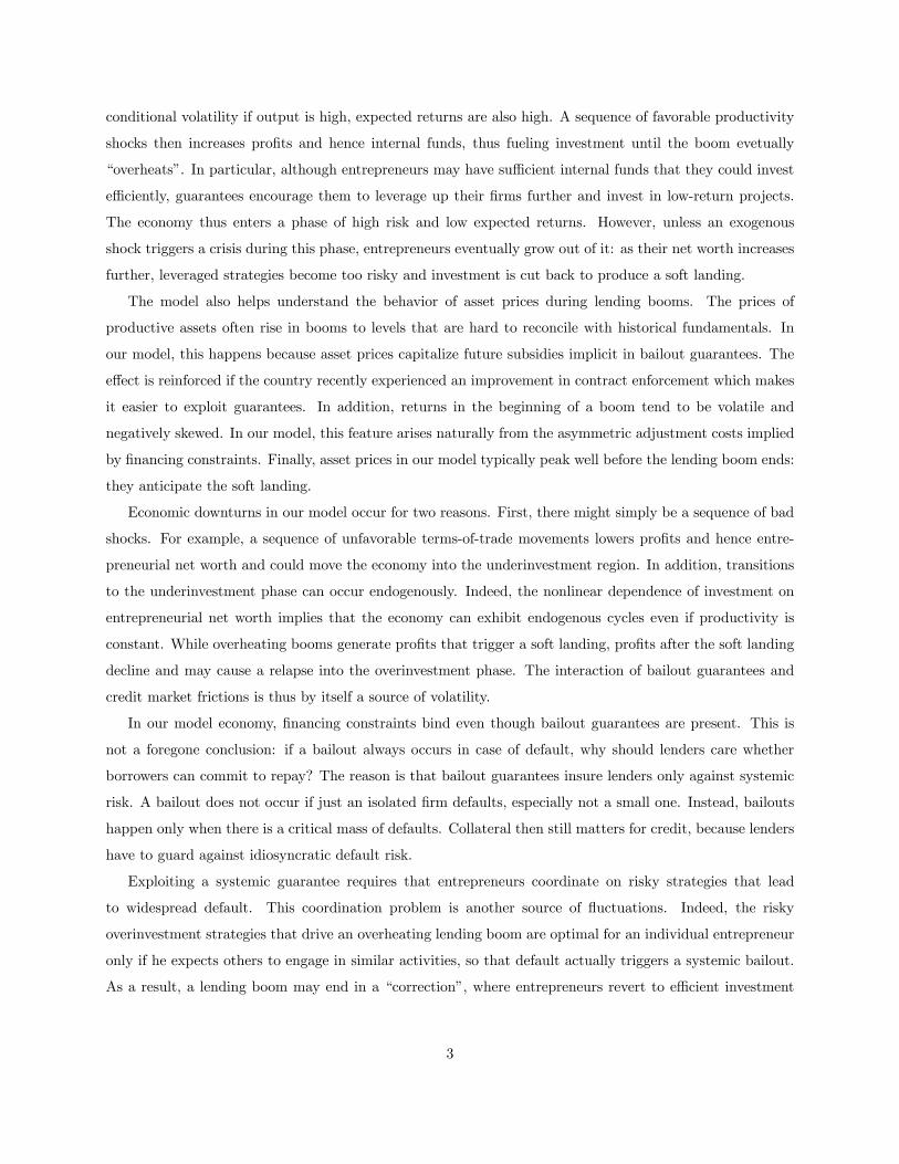
4.1. Stable Soft Landings

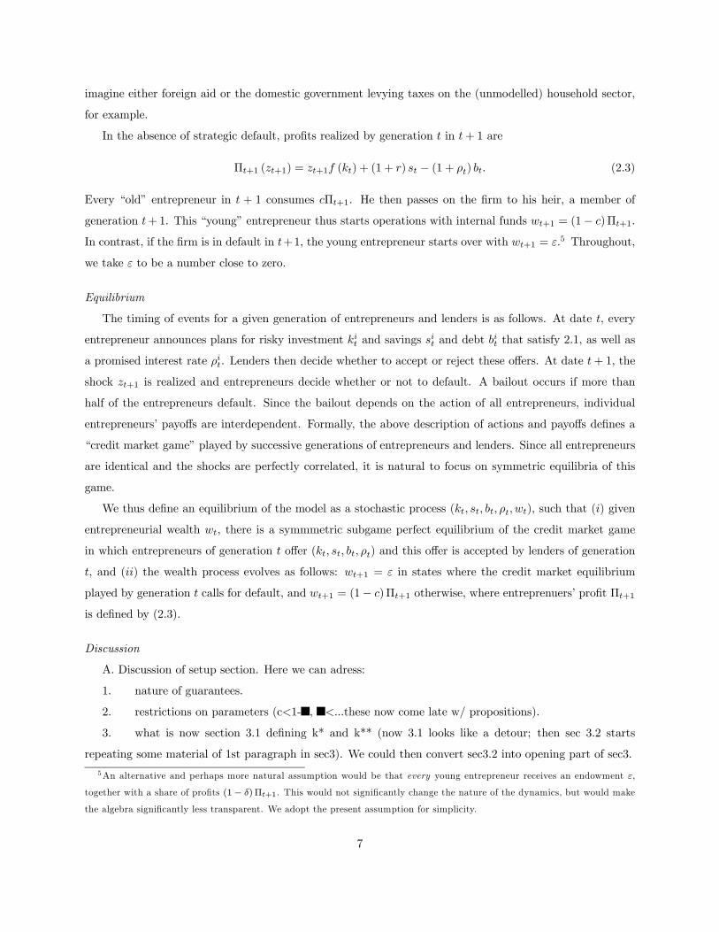
The case of stable soft landings — case (a) of Proposition 4.1 — is illustrated in Figures 4.1 and 4.2. This case

is relevant when the dividend rate is not too high. It describes economies where any lending boom that is

not punctured by a crisis ends in a soft landing. Moreover, every soft landing ushers in a phase of stability

that can only be ended by a crisis, that is, a bad productivity shock.

Mechanics

Figure 4.1 depicts the transition functions for internal funds (4.1) under two realization of the productivity

shock. Parameters are chosen so that they fall into case (a) of Proposition 4.1: in particular, the dividend

payout rate c is not too high. The top, solid, line in the figure is the transition function if the economy

remains on the lucky path (zt+1 = 1). There is always a discontinuity at wt = w∗, the boundary between

the multiple equilibria region, where a risky equilibrium is played, and the safe region. Since w∗ > k∗, the

risky equilibrium played at w = w∗ entails overinvestment, that is k > k∗. As w becomes larger than w∗, we

17

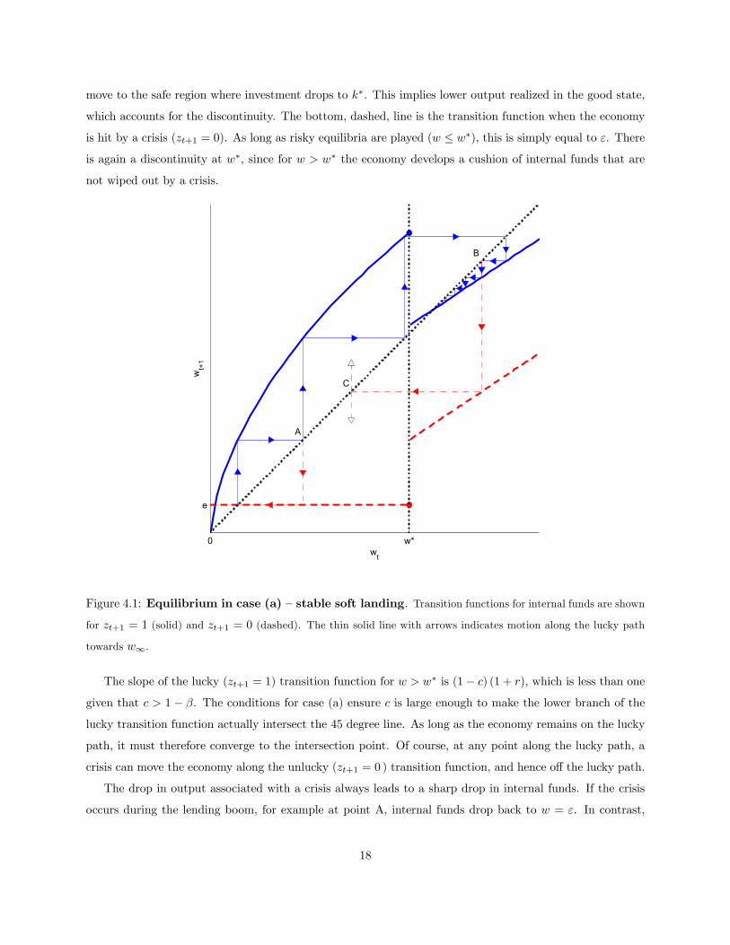
move to the safe region where investment drops to k∗. This implies lower output realized in the good state,

which accounts for the discontinuity. The bottom, dashed, line is the transition function when the economy

is hit by a crisis (zt+1 = 0). As long as risky equilibria are played (w ≤ w∗), this is simply equal to ε. There

is again a discontinuity at w∗, since for w > w∗ the economy develops a cushion of internal funds that are

not wiped out by a crisis.

0 w*

e

wt

wt+

1

A

B

C

Figure 4.1: Equilibrium in case (a) — stable soft landing. Transition functions for internal funds are shown

for zt+1 = 1 (solid) and zt+1 = 0 (dashed). The thin solid line with arrows indicates motion along the lucky path

towards w∞.

The slope of the lucky (zt+1 = 1) transition function for w > w∗ is (1− c) (1 + r), which is less than one

given that c > 1− β. The conditions for case (a) ensure c is large enough to make the lower branch of the

lucky transition function actually intersect the 45 degree line. As long as the economy remains on the lucky

path, it must therefore converge to the intersection point. Of course, at any point along the lucky path, a

crisis can move the economy along the unlucky (zt+1 = 0 ) transition function, and hence off the lucky path.

The drop in output associated with a crisis always leads to a sharp drop in internal funds. If the crisis

occurs during the lending boom, for example at point A, internal funds drop back to w = ε. In contrast,

18

if the economy was previously in the safe region, such as at point B, firms have a cushion of internal funds

that tempers the fall. Nevertheless, it is apparent from the figures that a finite sequence of crises is always

sufficient to return the economy to w = ε (in the figure, suppose that a second crisis occurs immediately

after the first crisis has moved the economy to point C). This property essentially guarantees existence of a

unique invariant distribution, as shown in the Appendix.

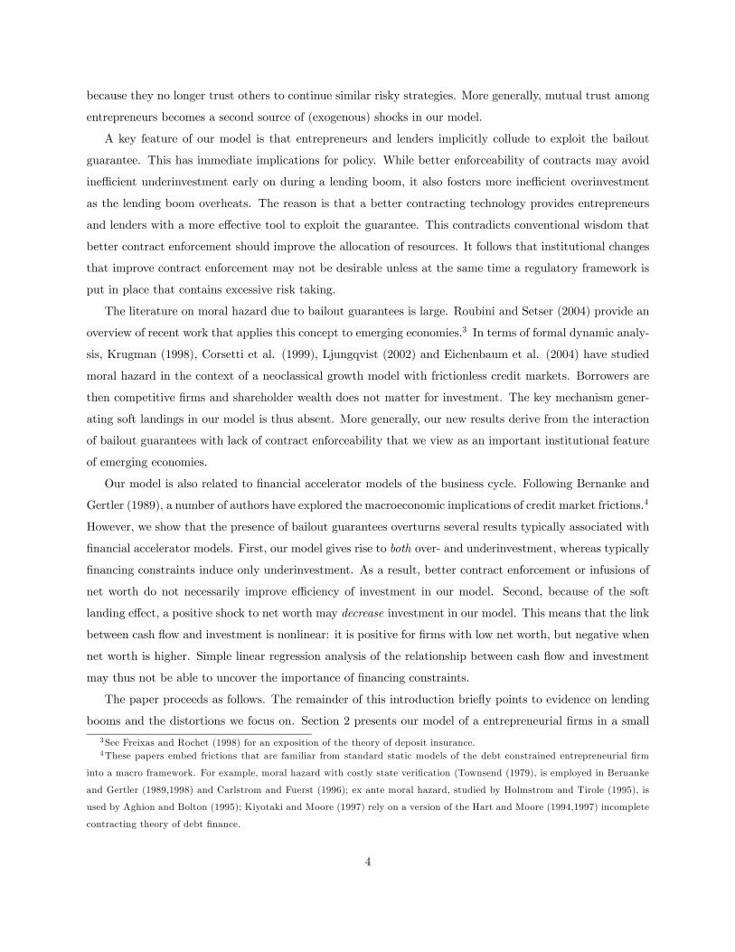
Intuition

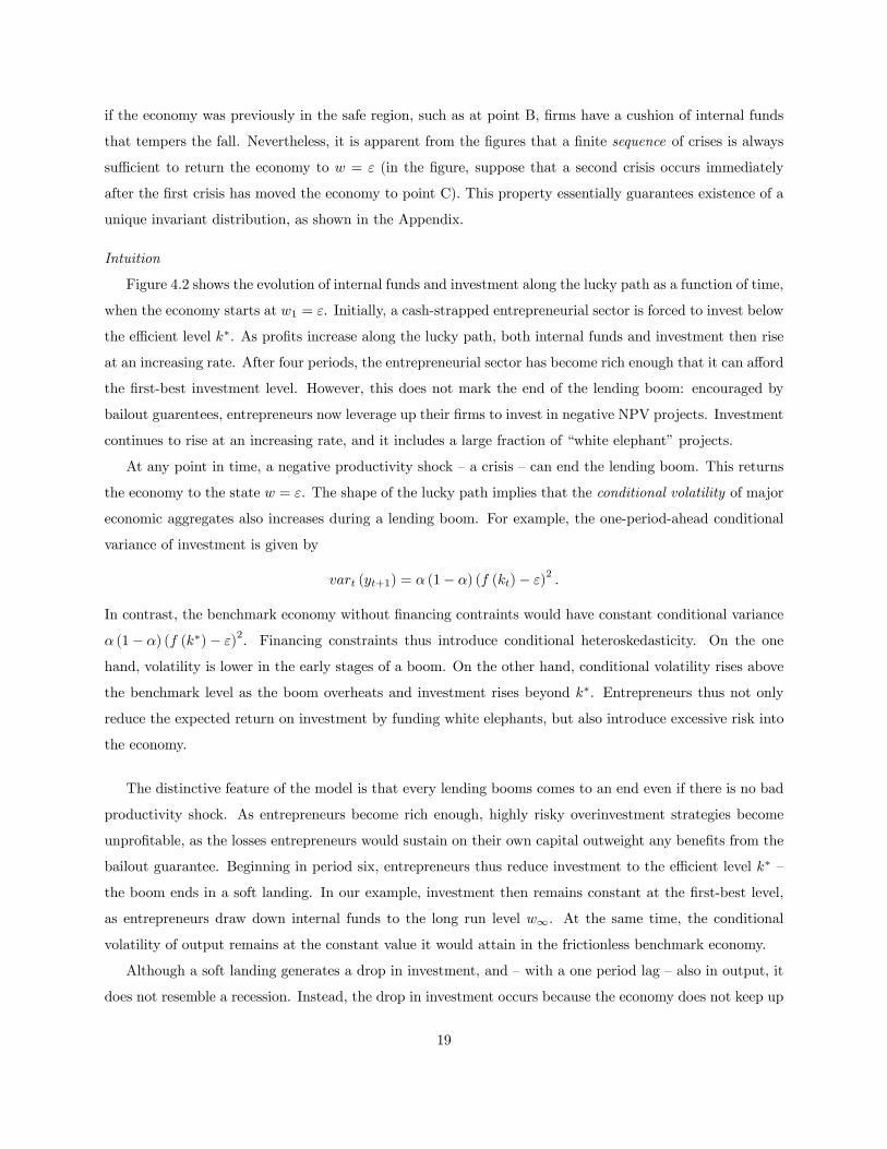
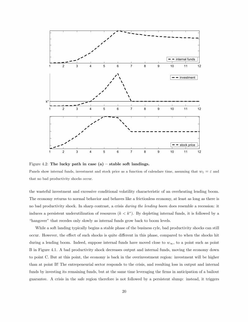
Figure 4.2 shows the evolution of internal funds and investment along the lucky path as a function of time,

when the economy starts at w1 = ε. Initially, a cash-strapped entrepreneurial sector is forced to invest below

the efficient level k∗. As profits increase along the lucky path, both internal funds and investment then rise

at an increasing rate. After four periods, the entrepreneurial sector has become rich enough that it can afford

the first-best investment level. However, this does not mark the end of the lending boom: encouraged by

bailout guarentees, entrepreneurs now leverage up their firms to invest in negative NPV projects. Investment

continues to rise at an increasing rate, and it includes a large fraction of “white elephant” projects.

At any point in time, a negative productivity shock — a crisis — can end the lending boom. This returns

the economy to the state w = ε. The shape of the lucky path implies that the conditional volatility of major

economic aggregates also increases during a lending boom. For example, the one-period-ahead conditional

variance of investment is given by

vart (yt+1) = α (1− α) (f (kt)− ε)2.

In contrast, the benchmark economy without financing contraints would have constant conditional variance

α (1− α) (f (k∗)− ε)2. Financing constraints thus introduce conditional heteroskedasticity. On the one

hand, volatility is lower in the early stages of a boom. On the other hand, conditional volatility rises above

the benchmark level as the boom overheats and investment rises beyond k∗. Entrepreneurs thus not only

reduce the expected return on investment by funding white elephants, but also introduce excessive risk into

the economy.

The distinctive feature of the model is that every lending booms comes to an end even if there is no bad

productivity shock. As entrepreneurs become rich enough, highly risky overinvestment strategies become

unprofitable, as the losses entrepreneurs would sustain on their own capital outweight any benefits from the

bailout guarantee. Beginning in period six, entrepreneurs thus reduce investment to the efficient level k∗ —

the boom ends in a soft landing. In our example, investment then remains constant at the first-best level,

as entrepreneurs draw down internal funds to the long run level w∞. At the same time, the conditional

volatility of output remains at the constant value it would attain in the frictionless benchmark economy.

Although a soft landing generates a drop in investment, and — with a one period lag — also in output, it

does not resemble a recession. Instead, the drop in investment occurs because the economy does not keep up

19

1 2 3 4 5 6 7 8 9 10 11 12

internal funds

1 2 3 4 5 6 7 8 9 10 11 12

k*

investment

1 2 3 4 5 6 7 8 9 10 11 12

stock price

Figure 4.2: The lucky path in case (a) — stable soft landings.

Panels show internal funds, investment and stock price as a function of calendare time, assuming that w1 = ε and

that no bad productivity shocks occur.

the wasteful investment and excessive conditional volatility characteristic of an overheating lending boom.

The economy returns to normal behavior and behaves like a frictionless economy, at least as long as there is

no bad productivity shock. In sharp contrast, a crisis during the lending boom does resemble a recession: it

induces a persistent underutilization of resources (k < k∗). By depleting internal funds, it is followed by a

“hangover” that recedes only slowly as internal funds grow back to boom levels.

While a soft landing typically begins a stable phase of the business cyle, bad productivity shocks can still

occur. However, the effect of such shocks is quite different in this phase, compared to when the shocks hit

during a lending boom. Indeed, suppose internal funds have moved close to w∞, to a point such as point

B in Figure 4.1. A bad productivity shock decreases output and internal funds, moving the economy down

to point C. But at this point, the economy is back in the overinvestment region: investment will be higher

than at point B! The entrepeneurial sector responds to the crisis, and resulting loss in output and internal

funds by investing its remaining funds, but at the same time leveraging the firms in anticipation of a bailout

guarantee. A crisis in the safe region therefore is not followed by a persistent slump: instead, it triggers

20

another overheated lending boom.

0 w*

e

wt

wt+

1

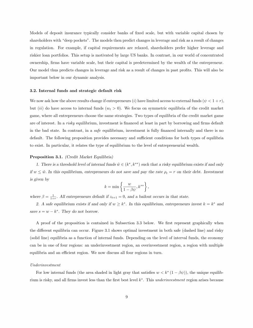
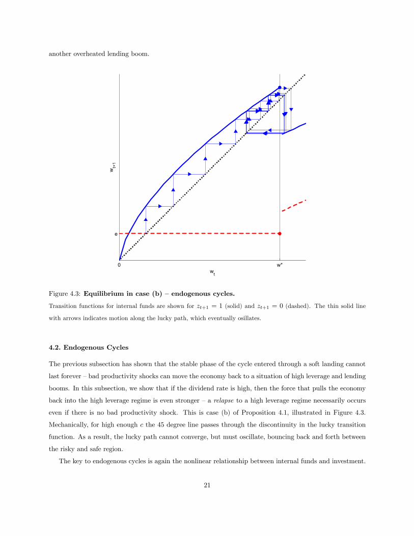
Figure 4.3: Equilibrium in case (b) — endogenous cycles.

Transition functions for internal funds are shown for zt+1 = 1 (solid) and zt+1 = 0 (dashed). The thin solid line

with arrows indicates motion along the lucky path, which eventually osillates.

4.2. Endogenous Cycles

The previous subsection has shown that the stable phase of the cycle entered through a soft landing cannot

last forever — bad productivity shocks can move the economy back to a situation of high leverage and lending

booms. In this subsection, we show that if the dividend rate is high, then the force that pulls the economy

back into the high leverage regime is even stronger — a relapse to a high leverage regime necessarily occurs

even if there is no bad productivity shock. This is case (b) of Proposition 4.1, illustrated in Figure 4.3.

Mechanically, for high enough c the 45 degree line passes through the discontinuity in the lucky transition

function. As a result, the lucky path cannot converge, but must oscillate, bouncing back and forth between

the risky and safe region.

The key to endogenous cycles is again the nonlinear relationship between internal funds and investment.

21

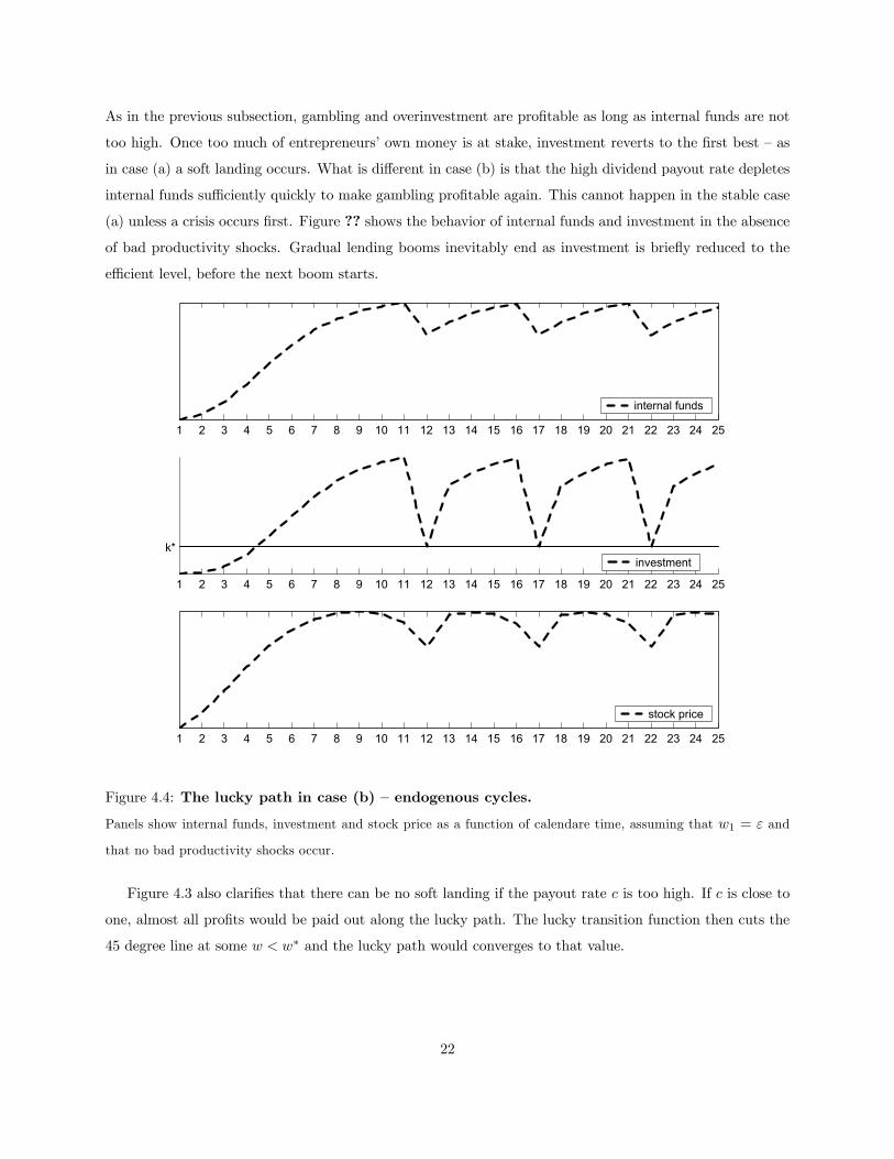
As in the previous subsection, gambling and overinvestment are profitable as long as internal funds are not

too high. Once too much of entrepreneurs’ own money is at stake, investment reverts to the first best — as

in case (a) a soft landing occurs. What is different in case (b) is that the high dividend payout rate depletes

internal funds sufficiently quickly to make gambling profitable again. This cannot happen in the stable case

(a) unless a crisis occurs first. Figure ?? shows the behavior of internal funds and investment in the absence

of bad productivity shocks. Gradual lending booms inevitably end as investment is briefly reduced to the

efficient level, before the next boom starts.

1 2 3 4 5 6 7 8 9 10 11 12 13 14 15 16 17 18 19 20 21 22 23 24 25

internal funds

1 2 3 4 5 6 7 8 9 10 11 12 13 14 15 16 17 18 19 20 21 22 23 24 25

k*investment

1 2 3 4 5 6 7 8 9 10 11 12 13 14 15 16 17 18 19 20 21 22 23 24 25

stock price

Figure 4.4: The lucky path in case (b) — endogenous cycles.

Panels show internal funds, investment and stock price as a function of calendare time, assuming that w1 = ε and

that no bad productivity shocks occur.

Figure 4.3 also clarifies that there can be no soft landing if the payout rate c is too high. If c is close to

one, almost all profits would be paid out along the lucky path. The lucky transition function then cuts the

45 degree line at some w < w∗ and the lucky path would converges to that value.

22

4.3. Stock Price Behavior

In recent boom-bust episodes, stock prices have often peaked well before a crisis. At the same time, crises

have proved remarkably hard to predict using financial indicators. How can these seemingly contradictory

facts be reconciled? We now show that the model suggests a natural explanation. To define stock prices, we

need to describe the financial policy of entrepreneurs in more detail. The analysis of section 3 assumes that

there is only inside equity, and that all external financing is obtained in the debt market. Here we define

dividends and price a claim to a dividend stream that we call outside equity. The interpretation is that there

is a — negligible — set of minority shareholders, who buy and sell outside equity in the stock market, while

the majority ownership remains with the entrepreneur. Since investors are risk neutral, the dividend stream

will be worth exactly its expected present value.

We assume that the entrepreneur runs a company that produces output, but that his other wealth is not

held within the company, and is therefore not used to pay dividends in times of crisis. Outside equity is a

claim to the profits delivered by the physical investment projects:

dt+1 = zt+1 (f (kt)− (1 + r) kt) .

If there is a bad productivity shock, no dividend is paid. In addition, in any crisis (that is, if zt+1 = 0)

the company is reorganized and outside equity becomes worthless. Of course, the entrepreneur, who is

the controlling shareholder of the firm, may recapitalize the company in a crisis — this is what happens in

the safe region, where the entrepreneur actually has sufficient funds to avert default. Nevertheless, outside

equityholders receive zero in any crisis.7

This setup leads to a simple recursion for the stock price along the lucky path. Let P0 denote the stock

price in the state w = ε. Then Pn, the stock price in the nth period that the economy remains on the lucky

path can be found from

Pn = βα (f (kn)− (1 + r) kn + Pn+1) ,

where kn is investment along the lucky path. This path for the stock price is plotted in the third panels of

Figures 4.2 and 4.4.

The two plots shed light on the whole evolution of stock prices. In the risky region, the stock price moves

along the lucky path until a crisis occurs, at which point it reverts to P0. Throughout the safe region, the

stock price is constant atβα

1− αβ(f (k∗)− (1 + r) k∗) .

7An alternative scenario would be to have the entrepreneur’s wealth as a part of the firm’s asset. One could then define

dividends as proportional to total entrepreneurial profits. Given the limited power of minority shareholders in many middle

income countries, it seems more natural to assume that minority shreholders lose out in a crisis.

23

Any transition from the safe to the risky region caused by a crisis or a reversal implies a restart of the

recursion. While we do not show separate numerical results for this case, it is clear from the recursion

formula that any price sequence that follows a crisis or relapse must have the same qualitative features as

the stock market boom that starts in the state w = ε.

A key feature of the model is that the stock price peaks before a soft landing occurs. This is because

asset prices are forward looking — they factor in the lower dividends the company expects to pay after a soft

landing. In the safe region, no bailout is expected — and the controlling shareholders — the entrepreneurs —

have to recapitalize the firm in case of default. The resulting cutback of investment lowers dividends in the

good state, while dividends are always zero in the bad state. Therefore, expected dividends fall.

The hump shape of the lucky stock price path helps understand why prices can peak before a crisis. Any

country that experiences a crisis while being far enough along the lucky path will exhibit such a pattern.

However, this does not mean that a peak of the stock market helps predict a crisis. Indeed, in our model the

incidence of a crisis is an iid event, so that knowledge of the stock price does not help forecast it. The peak

only signals that a soft landing is now closer — it tells investors nothing about future productivity shocks.

4.4. Fluctuations in Trust

The analysis so far has abstracted from fluctuations in trust by assuming that xt ≡ r, that is, entrepre-

neurs coordinate on a risky credit market equilibrium whenever such an equilibrium exists. The following

proposition characterizes equilibria when this assumption is relaxed.

Proposition 4.2. (Fluctuations in Trust)

Suppose that ε < (1− βψ) k∗ and c > 1− β.

1. For any stationary Markov trust process {xt} , independent of {zt}, there is a unique stationaryequilibrium.

2. (Minimum Risk Equilibria) Suppose xt is held constant at xt = s. There are thresholds c3 and c4,

with c1 < c3 < c4 < 1, that define three cases for the lucky path

(a) if c ≤ c3, internal funds converge along the lucky path to a constant w∞.

(b) if c ∈ (c3, c4], internal funds oscillate between the risky and safe region.(c) if c > c4 > c2, the lucky path converges to a constant in the risky region.

3. In any state (w, x) where there is low trust (x = s), the 1-period-ahead conditional variances of internal

funds, investment and output are smaller than in the corresponding state of high trust (x = r).

Part 1 of the Prosposition says that adding exogenous shocks to trust does not change the basic nature

of the dynamics. An equilibrium is described by a stationary Markov equilibrium; in this respect the model

resembles standard business cycle models. The difference to Proposition 4.1 is that there are now two

24

exogenous forcing processes — productivity shocks {zt} and trust, which does not affect payoffs directly.However, it can matter for real activity, because it acts as a coordination device for entrepreneurs. Formally,

the equilibrium may thus be viewed as a stochastic sunspot equilibrium.

The new transition functions for internal funds are illustrated in Figure 4.5. This figure resembles Figure

4.1. The top solid black line is still the unique lucky transition function in the range wt < k∗. In the multiple

equilibria region wt ∈ [k∗, w∗], the solid black line is the lucky transition function that is relevant when trustis high, xt = r. The cases of Proposition 4.1 thus remain relevant for understanding the dynamics when

xt = r — for the figure, we have chosen a consumption rate c that lies below c2. What is new relative to

Figure 4.1 is that there is now a separate lucky transition function that becomes relevant when xt = s. This

lucky transition function is the dotted black line defined over the range [k∗, w∗]. Similarly, there is an unlucky

transition function for xt = s, drawn as a dotted gray line. In any state within the multiple equilibria region,

the level of trust determines which pair of transition functions is relevant. The shock zt+1 then selects the

lucky or unlucky transition from the relevant pair.

To understand the dynamics in general it is helpful to focus first on minimum risk equilibria. These

occur when xt ≡ s: a safe credit market equilibrium is played whenever it exists. Minimum risk equilibria

are thus the polar opposite of the maximum risk equilibria of Proposition 4.1. They minimize the risk

taking potential of bailout guarantees because entrepreneurs do not trust each other enough to coordinate

risk taking. Part 2 of Proposition 4.2 characterizes the lucky path in a minimum risk equilibrium. The

argument parallels that for maximum risk equilibria. Indeed, the transition functions for a minimum risk

equilibrium have discontinuities at w = k∗, just like the transition function for a maximum risk equilibrium

had discontinutities at w = w∗.

In the figure, the lucky transition function for the case xt = s is above the 45 degree line at w = k∗. This

implies that we are in case (a) of Proposition 4.2. The lucky path in a minimum risk equilibrium, drawn

as a thin solid line with arrows, converges to a constant. Along the lucky path investment first increases,

possibly beyond the efficient level. However, it quickly reaches the safe region of efficient investment. The

entrepreneurial sector then proceeds to accumulate a cushion of internal funds. In the present example, this

cushion eventually becomes large enough that a single crisis cannot displace the economy out of the safe

region! In other words, the economy can withstand a bad productivity shock, keeping investment at the

efficient level in its aftermath. Of course, a sufficiently long sequence of bad productivity is always sufficient

to move the economy back to the risky region.

The gray dashed line illustrates some of the additional dynamics that are possible when trust fluctuates.

The two paths coincide up to the point A. However, at this point the dashed path represents what happens

with high trust: investment is much higher than in the minimum risk equilibrium (the solid path). If

entrepreneurs’ gamble is successful and the economy remains on the lucky path, growth is much higher than

25

0 k* w*

e

wt

wt+

1

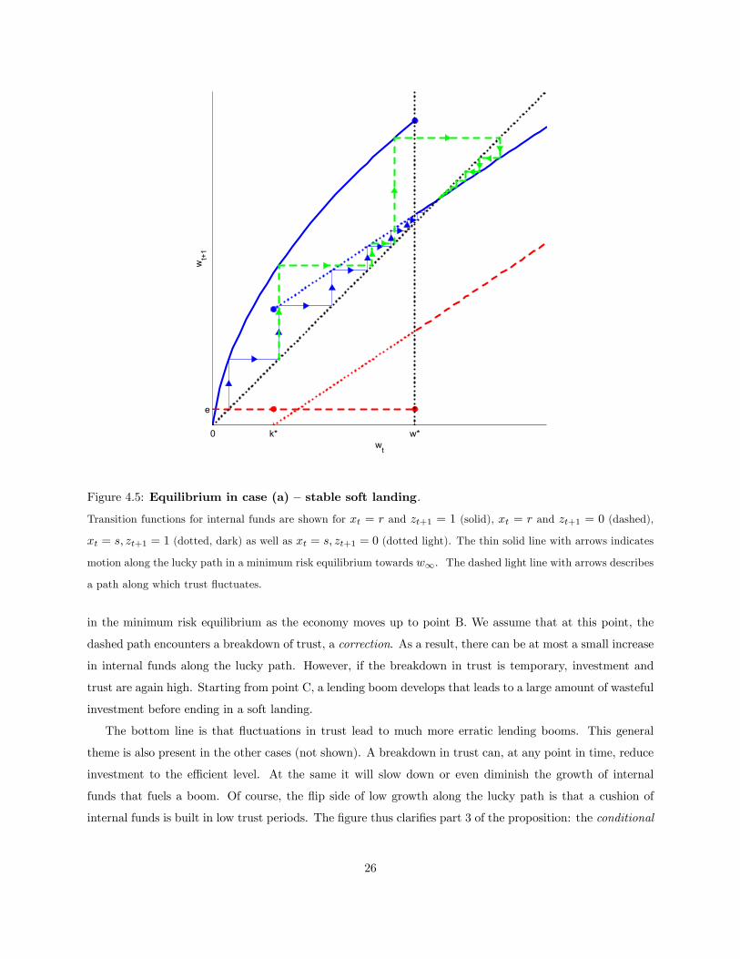
Figure 4.5: Equilibrium in case (a) — stable soft landing.

Transition functions for internal funds are shown for xt = r and zt+1 = 1 (solid), xt = r and zt+1 = 0 (dashed),

xt = s, zt+1 = 1 (dotted, dark) as well as xt = s, zt+1 = 0 (dotted light). The thin solid line with arrows indicates

motion along the lucky path in a minimum risk equilibrium towards w∞. The dashed light line with arrows describes

a path along which trust fluctuates.

in the minimum risk equilibrium as the economy moves up to point B. We assume that at this point, the

dashed path encounters a breakdown of trust, a correction. As a result, there can be at most a small increase

in internal funds along the lucky path. However, if the breakdown in trust is temporary, investment and

trust are again high. Starting from point C, a lending boom develops that leads to a large amount of wasteful

investment before ending in a soft landing.

The bottom line is that fluctuations in trust lead to much more erratic lending booms. This general

theme is also present in the other cases (not shown). A breakdown in trust can, at any point in time, reduce

investment to the efficient level. At the same it will slow down or even diminish the growth of internal

funds that fuels a boom. Of course, the flip side of low growth along the lucky path is that a cushion of

internal funds is built in low trust periods. The figure thus clarifies part 3 of the proposition: the conditional

26

volatility of real variables is reduced in low trust periods.

5. Appendix

Proof of Proposition 3.1.

We have defined a safe plan as a plan with bt = 0, and a risky plan as a plan with st = 0, bt > 0 and

default in the bad, but not in the good state. We first show that entrepreneurs never pick any other plans,

whether or not a bailout is expected in the bad state. Given this fact, it is sufficient to show that (i) when

a bailout is expected, a risky plan is optimal if and only if w ≤ w∗, and (ii) when no bailout is expected, a

safe plan is optimal if and only if w ≥ k∗. Claim (ii) is established in the text. An analytical proof of claim

(i) that does not rely on the graphical argument in the text, is offered below.

Step 1: Only safe or risky plans can ever be optimal.

First, it never makes sense to offer a plan that leads to default for sure. Whether or not there is a bailout

in the bad state, lenders will accept such a plan only if they obtain at least 1+ r per dollar lent in the good

state. However, they can only seize this much if all the borrowed funds are invested in riskless savings — after

all, they can only recover ψ < 1 + r per dollar invested in capital. But if entrepreneurs invest all borrowed

funds in savings, they make zero profits on these funds and might as well not borrow.

Second, inspection of the conditions for default show that there does not exist a plan under which default

is optimal in the good state, but not in the bad state.

We are thus left with plans that either (i) never default, or (ii) default in the bad state, but not in the

good state. We show that for both types, without loss of generality, borrowing and riskless saving can be

taken to be mutually exclusive activities.

Indeed, any savings are seized by lenders in case of default. This means that the expected return on a

dollar saved under a type (ii) plan is α (1 + r) . At the same time, the expected cost of a dollar borrowed is

α (1 + r) when a bailout is expected (and 1 + r must only be paid in the good state), and it is 1 + r when

no bailout is expected. Therefore, saving a borrowed dollar never leads to positive profits under a type (ii)

plan. Since type (i) plan triggers default in the good state, it must necessarily involve some borrowing. The

previous argument implies that wlog it can be taken to be a risky plan (with st = 0).

Under a type (i) plan, the expected return on a dollar saved or invested cannot be less than 1+ r. At the

same time, the expected cost of a dollar borrowed is 1 + r whether or not a bailout is expected (the bailout

does not affect a safe plan that does not lead to default). Again, saving a borrowed dollar cannot lead to

positive profits. A type (ii) plan that involves borrowing must necessarily involve some riskless savings, since

otherwise could not be paid in the bad state. The previous argument thus implies that wlog borrowing can

be taken to be zero, so that the type (i) plan can be taken to be a safe plan.

27

Step 2: When a bailout is expected, a risky plan is optimal if and only if w ≤ w∗, for some w ∈ (k∗, k∗∗) .The profit functions for the best safe and risky plan, derived in the text, are

V (ks (w) , w) =

αf(w) if w ≤ k∗

αf(k∗) + (1 + r) (w − k∗) if w > k∗(5.1)

V (kr(w) , w) =

αf( w1−βψ )− α ψw

1−βψ if w ≤ k∗∗[1− βψ]

αf(ek) + α (1 + r)hw − eki if k∗∗ > w > k∗∗[1− βψ]

(5.2)

The following lemma characterize these functions and thereby complete the proof.

Lemma 5.1. If f 0(0) > 1 + r, then πr(w) > πs(w) for any w on (0, k∗].

Proof. Define the function Π(w) = πr(w)− πs(w) on [0, k∗] . Equations (5.1) and (5.2) imply that Π(w)

is continuous. There are two cases. First, in the case k∗ ≤ k∗∗[1− βψ]

Π(w) = α [f (kr)− f(w)]− α (1 + r) [kr − w] , w ∈ (0, k∗] (5.3)

where kr = w1−βψ . The mean value theorem implies that there exists a constant a ∈ (w, kr) such that

βf 0(a) = β f(kr)−f(w)kr−w . Concavity of f implies that βf 0(a) > βf 0(kr) ≥ βf 0( k∗

1−βψ ) ≥ βf 0(k∗∗) = 1. Since

βf 0(a) > 1, it follows that (5.3) is positive for any w on (0, k∗].

Consider now the case k∗ > k∗∗[1− βψ]. For w ≤ k∗∗[1− βψ] the argument is the same as the previous

one. For w > k∗∗[1− βψ] replace kr by k∗∗ in (5.3), and note that there is a constant b ∈ (w, k∗∗) such thatβf 0(b) = β f(k∗∗)−f(w)ek−w . Moreover, βf 0(b) > 1 because b < k∗∗.¤

Lemma 5.2. There is a unique wealth level ew(ψ) such that πr(w) < πs(w) if and only if w > ew(ψ).Furthermore, ew(ψ) > k∗∗(1− βψ) if and only if ψ > eψ, where

eψ ≡ αβ[f(k∗)−f(k∗∗)]−[k∗−k∗∗][1−α]βk∗∗ < 1

β (5.4)

Proof. We consider first the case k∗ ≤ k∗∗(1 − βψ) ≡ w̄. Equations (5.1) and (5.2) imply that Π(w)

has the following three properties. First, for w ≥ k∗, Π(w) is concave. That is, Π0(w) is declining. Second,

Π0(w) is negative for any w ≥ w̄. Third, Π(w̄) > 0 if and only if ψ > eψ. It follows that there is a unique ewsuch that Π( ew) = 0. Furthermore, for ψ > (<)eψ, we must have ew(ψ) > (<)k∗∗(1− βψ).

We consider now the case w̄ < k∗. Lemma 5.1 implies that Π(w̄) > 0. Since Π0(w) < 0 for w ≥ w̄, there

is a unique ew such that Π( ew) = 0. Furthermore, ew > k∗ > w̄.

Finally, we show that eψ < β−1. The mean value theorem implies that there is a constant a ∈ (k∗, k∗∗)such that eψ ≡ 1−αβf 0(a)

[1−α]βk∗∗/[k∗∗−k∗] . Since, βf0(a) > βf 0(k∗∗) = 1, we have that eψ < [1−α][k∗∗−k∗]

[1−α]βk∗∗ < 1β . The

second inequality follows from ek > k∗.¥

28

Proof of Proposition 4.1.

It is useful to first prove the properties of the lucky path in part 2.

Part 2. Define the thresholds c1 and c2 as follows:

(1− c1) (f(k∗) + (1 + r) (w∗ − k∗)) = w∗, (5.5)

(1− c2)

µf(min

½w∗

1− βψ, k∗∗

¾) + (1 + r)

µw∗ −min

½wt

1− βψ, k∗∗

¾¶¶= w∗. (5.6)

In terms of Figure ??, c1 is the unique value of c for which the lower branch of the lucky transition function

intersects the 45 degree line exactly at w = w∗. Also, c2 is the unique value of c for which the upper branch

intersects the 45 degree line at w∗.

We have c1 > 1− β. Indeed, suppose that c = 1− β. By (4.1), the lower branch of the lucky transition

function is always above the 45 degree line at w = w∗:

(1− c) (f(k∗) + (1 + r) (w∗ − k∗)

= w∗ + βf (k∗)− k∗

> w∗ + β (αf (k∗)− (1 + r) k∗)

> w∗,

where the last inequality follows from the fact that f is continuous and concave, αf 0 (0) > 1 + r and

αf 0 (k∗) = (1 + r) . Now varying c does not affect the optimal plans or what equilibrium is played — all it

does is scale the lucky transition function. Therefore, there must exist c1 with β > 1− c1 > 0 such that (5.5)holds.

We also have c2 > c1. Indeed, the best risky plan for w = w∗ derived in the proof of Proposition 3.1

maximizes f(k) + (1 + r) (w∗ − k) subject to the collateral contraint (1− βψ) k ≤ w∗. But k = k∗ was in

the contraint set of this problem since Proposition 3.1 implies that w∗ > k∗. Therefore,µf(min

½w∗

1− βψ, k∗∗

¾) + (1 + r)

µw∗ −min

½w∗

1− βψ, k∗∗

¾¶¶> (f(k∗) + (1 + r) (w∗ − k∗)) .

As a result, there must exist c2 with 1−c1 > 1−c2 > 0 such that (5.6) holds. Graphically, the upper branchof the lucky transition function is always strictly above the lower branch at w = w∗.

Consider c ∈ (1− β, c2). Since the upper branch is strictly above the 45 degree line for all w ≤ w∗,

the lucky path must grow beyond w∗ — there must be a soft landing. Cases a and b distinguish different

behaviors inside the safe region (w > w∗).

First. consider c ∈ (1−β, c1). In this case, the lower branch of the lucky transition function is above the

45 degree line. The slope of the lower branch is (1− c) (1 + r) < 1, so that the lower branch must cut the 45

degree line from above at some value w∞ > w∗. Therefore, within the safe region, the lucky path converges

to w∞. For c = c1, we have w∞ = w∗, that is the lucky path converges to w∗. This establishes case a.

29

Second, consider c ∈ (c1.c2). In this case, the lower branch is below the 45 degree line at w = w∗, whereas

the upper branch remains above it — the lucky transition function does not intersect the 45 degree line at all.

In addition, for w > w∗, the fact that the slope of the lower branch is less than one implies that wt decreases

monotonically. Since the lower branch is strictly below w∗ at w = w∗, it follows that the lucky path must

again transit to w < w∗. In this region, it will again monotonically increase until it must transit to w > w∗

and so on. This establishes case b.

Finally, consider c ≥ c2. The lucky transition function cuts the 45 degree from above at some w∞ with

0 < w∞ < w∗. Therefore, the lucky path increases monotonically and converges to w∞, and therefore it

never reaches the safe region.

(1− c)³f(min

nw∗1−βψ , k

∗∗o) + (1 + r)

³w∗ −min

nw∗1−βψ , k

∗∗o´´

Part 1. Step 1. There is a number w̄, such that the process {wt} lives on the interval [ε, w̄].The upper bound w̄ is defined as follows. Let w∞ denote the largest value where the lucky transition

function crosses the 45 degree line and define

whi := (1− c)

µf(min

½w∗

1− βψ, k∗∗

¾) + (1 + r)

µw∗ −min

½w∗

1− βψ, k∗∗

¾¶¶,

the value of the lucky transition function at w = w∗. Now define w̄ = max©whi, w∞

ª.

We now show that the upper bound w̄ is respected by any sample path that starts in [ε, w̄] and for which

the shock realization is zt = 1 throughout. We verify this separately for the parametrizations of cases a-c.

In case c, w∞ ∈ (0, w∗). We must have w ≤ w∞, because all paths starting at w < w∞ converge

monotonically to w∞ from below.

In case b, w∞ = 0. However, as shown in the proof of part 1, any path must be decreasing in the safe

region. Therefore, w ≤ whi, since whi is the highest point at which a path can possibly enter the safe region.

In case a, there can be two subcases. If w∞ ≥ whi, then all paths converge monotonically to w∞ from

below. In contrast, if w∞ < whi then there exist paths that enter the safe region at w > w∞. However, the

slope of the lower branch of the lucky path all paths must be monotonically decreasing as they converge to

w∞. Therefore we have w ≤ whi as in case b.

It remains to show that sample paths that experience crises (zt = 0) at least once also respect the upper

bound. But holdings fixed wt, a crisis outcome of wt+1 is always strictly below the outcome if there is no

crisis. Therefore all sample paths respect the upper bound.

Finally, it is clear that wt ≥ ε: since ε < (1− βψ) k∗, the lucky path is monotonically increasing at

w = ε, while the outcome for w in a crisis is bounded below by ε.

Step 2. There is an integer n and a number γ > 0 such that, for every point v ∈ [ε, w̄] ,

Pr (wt+N = ε|wt = v) > γ.

30

To construct γ and n, consider first v ∈ (w∗, w̄]. We know that the “unlucky” transition function (for

zt+1 = 0) has a slope less than one and that its value at w = w∗ is

(1− c) (1 + r) (w∗ − k∗) < w∗ − k∗ < w∗,

so that it lies below the 45 degree line for all w > ε. This implies that for every v ∈ (w∗, w̄], a finite sequenceof crises (realizations zt = 0) — occurring one after the other — implies that wt returns to the region where

w < w∗. But for w ≤ w∗, a crisis wipes out all internal funds in that region so that Pr (wt+1 = ε|wt = v) =

1 − α. Therefore no more than a finite number of realizations zt = 0 leads from any v ∈ (w∗, w̄] to w = ε.

In particular, the most steps are required for v = w̄. We thus let N be the smallest integer such that

Pr (wt+N = ε|wt = w̄) = (1− α)N and pick γ = (1− α)

N/2.

For v < w̄, the smallest integer n such that Pr (wt+n = ε|wt = w̄) = (1− α)n is less or equal to N . (In

particular, for v < w∗, n = 1). Moreover, wt = ε and zt+1 = 0 implies wt+1 = ε, since the endowment is

always below w∗. Therefore, Pr (wt+N = ε|wt = w̄) is at least (1− α)N and thus by constrution larger then

γ.

Step 3. There is a unique invariant measure associated with the Markov operator defined by (4.1).

We verify the conditions of Theorem 11.10 in Stokey and Lucas (1989).

First, Step 2 implies that the Markov operator satisfies Doeblin’s condition: there is a finite measure φ

on the state space [ε, w̄], an integer N ≥ 1, and a number γ > 0, such that, for every Borel subset of [ε, w̄],

if φ (B) ≤ γ then Pr {wt+N ∈ B|wt = v} ≤ 1− γ for all v ∈ [ε, w̄]. Indeed, let φ be a Dirac measure on thepoint ε, that is φ ({ε}) = 1, φ (B) = 1 for all B such that ε ∈ B, and φ (B) = 0 for all B such that ε /∈ B.

Second, our construction of φ also implies that for any Borel set B of positive φ-measure (in our case,

any B containing ε), then for each v ∈ [ε, w̄], there is an integer n ≥ 1 such that Pr (wt+n = ε|wt = v) > 0.

Indeed, Step 2 has shown that the probability of reaching ε itself from any starting point v is positive.¥

Proof of Proposition 4.2.

Part 1. Step 1 in the proof of Proposition 4.1 goes through if the interval for internal funds wt is expanded

to (0, w̄]. Indeed, for given wt, the level wt+1 that obtains for zt+1 = 1 is bounded above by the value that

obtains if xt = r, the case covered in the proof of Proposition 4.1. This implies that the upper bound w̄ need

not change. The lower bound now becomes zero, since internal funds may drop below ε if a crisis occurs in a

safe equilibrium (cf. Figure 4.5). However, internal funds never reach zero, since wt+1 = ε whenever a crisis

reduces profits to zero.

Step 2 in the proof of Proposition goes through with minor modification. Indeed, one can follow the

above proof to construct an integer n and a number γ > 0 such that, for every point (v, x) ∈ [ε, w̄]× {r, s} ,Pr (wt+N = ε, xt+1 = r|wt = v, xt = x) > γ. The key to that step is that internal funds return to the value ε

31

in a finite number of steps. This can be engineered as before by selecting a sufficiently long sequence of crises.

Since x and z are indepdendent, an accompanying sequence of x values can be picked without upsetting this

key property.

Given the result of Steps 1 and 2, Step 3 can be applied to the Markov operator (4.1) as before.

Part 2. We define thresholds c3 and c4 by

(1− c3) f (k∗) = k∗

(1− c4)

µf(min

½k∗

1− βψ, k∗∗

¾) + (1 + r)

µk∗ −min

½wt

1− βψ, k∗∗

¾¶¶= k∗.

We have c3 > 1−β. Indeed, suppose that c = 1−β. Since k∗ is defined by αf 0 (k∗) = 1+ r, strict concavity

of f implies

(1− c) f (k∗) > (1− c) f 0 (k∗) k∗ = (1− c)1 + r

αk∗ > (1− c) (1 + r) k∗ = k∗.

Therefore, the lucky transition function in a safe equilibrium at w = k∗ which equals f (k∗) is above the 45

degree line if c = 1− β.

The equations defining c3 and c4 are the same as those defining c1 and c2 above, except that w∗ has been

replaced by k∗. Similar arguments as above imply that c4 > c3. In addition, w∗ > k∗ implies that c4 > c2

and c3 > c1.

Suppose now that xt = s always. The lucky transition function now has a discontinuity at w = k∗; it

follows the lucky safe transition function for all w ≥ k∗. The rest of the proof parallels the arguments in the

proof of Proposition 4.1

In case (a), the lower branch of the lucky transition function is above the 45 degree line. It follows that

the lucky path converges.

In case (b), the 45 degree line passes through the discontinuity in the lucky transition function. It follows

that the lucky path must oscillate. Finally, in case (c), the lucky transition function intersects the 45 degree

line at a point below k∗. The lucky path converges montonically to that point.¥

References

[1] Aghion, P. and P. Bolton (1997). “A Theory of Trickle-Down Growth and Development.” Review of

Economic Studies 64 151-172.

[2] Aghion, P., P. Bacchetta, and A. Banerjee (1998), Capital Markets and the Instability of Open

Economies, mimeo, Harvard University.

[3] Bekaert G. and C. Harvey (2003), “Emerging Markets Finance”, Journal of Empirical Finance 10, 3-55.

32

[4] Bernanke, B. and M. Gertler (1989). “Agency Costs, Collateral and Business Fluctuations.” American

Economic Review 79, 14-31.

[5] Bernanke, B., M. Gertler and S. Gilchrist. “The Financial Accelerator in a Quantitative Business Cycle

Framework.” NBER working paper 6455.

[6] Burnside, C., M. Eichenbaum and S. Rebelo (2004), Government Guarantees and Self-Fulfilling Specu-

lative Attacks, Journal of Economic Theory.

[7] Carlstrom, Charles and Timothy Fuerst (1997). “Agency Costs, Net Worth and Business Cycles: A

Computable General Equilibrium Analysis.” American Economic Review v87, n5, 893-910.

[8] Claessens, S, S. Djankov and L. Lang (1999), “Corporate Growth, Financing, and Risks in the Decade

before East Asia’s Financial Crisis”, mimeo, World Bank.

[9] Corsetti, P. Pesenti and N. Roubini (1998). “Paper Tigers,” European Economic Review v43, 1211-1236.

[10] Gourinchas, P. O., O. Landerretche, and R. Valdes (2001). “Lending Booms: Latin America and the

World”, Economia 1(2).

[11] Guerra, A. (1998). “Asset Inflation and Financial Crisis,” mimeo, Banco de Mexico.

[12] Hernandez, L. and O. Landerretche (1998) “Capital Inflows, Credit Booms and Macroeconomic Vulner-

ability: the Cross-country Experience” mimeo, Central Bank of Chile.

[13] Hart, O. and J. Moore (1994). “A Theory of Debt based on the Inalienability of Human Capital.”

Quarterly Journal of Economics 59, 841-79.

[14] Harvey, C., K. Lins, and A. Roper (2004), “The effect of capital structure when agency costs are

extreme”, Journal of Financial Economics 74, 3-30.

[15] Himmelberg, C., G. Hubbard and I. Love (2002), “Investor Protection, Ownership, and the Cost of

Capital”, mimeo, Columbia.

[16] Holmstrom, B. and J. Tirole (1997). “Financial Intermediation, Loanable Funds and the Real Sector.”

Quarterly Journal of Economics v 112, 663-691.

[17] Kiyotaki, N. and J. Moore (1997). “Credit Cycles.” Journal of Political Economy 105, 211-248.

[18] Klapper, L. and I. Love (2002), “Corporate Governance, Investor Protection, and Performance in Emerg-

ing Markets”, mimeo, World Bank.

[19] Krueger, A. and A. Tornell (1999). “The Role of Bank Restructuring in Recuperating From Crises:

Mexico 1995-98,” NBER working paper.

33

[20] Krugman, P. (1998). “Bubble, Boom, Crash: Theoretical Notes on Asia’s Crisis.” mimeo, MIT.

[21] Ljungqvist, L. (2002). “Government Guarantees on Assets and Volatility”, mimeo, Stockholm School of

Economics.

[22] Roubini, N. and B. Setser (2004), “Bailouts or Bail-ins? Responding to Financial Crises in Emerging

Economies”.

[23] Sachs, J., A. Tornell and A. Velasco (1996). “Financial Crises in Emerging Markets: The Lessons From

1995,” Brookings Papers on Economic Activity.

[24] Tornell A. (1999). “Common Fundamentals in the Tequila and Asian Crises,” NBER working paper.

[25] Townsend, R. “Optimal Contracts and Competitive Markets with Costly State Verification.” Journal

of Economic Theory 21, 265-93.

34