condition monitoring of a rotor bearing system
TRANSCRIPT

CONDITION MONITORING OF A ROTOR BEARING SYSTEM
Herbert Alfred Grobler
Submitted in fulfilment of the academic requirements for the degree of Master of Science in
Mechanical Engineering
December, 2011
Supervisor: Glen Bright
Co-Supervisor: Richard Loubser

ii
As the candidate’s Supervisor I agree/do not agree to the submission of this dissertation
Signed:………………………………… Date:……………………………
Professor Glen Bright

iii
DECLARATION
I Herbert Grobler declare that
(i) The research reported in this dissertation, except where otherwise indicated, is
my original work.
(ii) This dissertation has not been submitted for any degree or examination at any
other university.
(iii) This dissertation does not contain other persons’ data, pictures, graphs or other
information, unless specifically acknowledged as being sourced from other
persons.
(iv) This dissertation does not contain other persons’ writing, unless specifically
acknowledged as being sourced from other researchers. Where other written
sources have been quoted, then:
a) their words have been re-written but the general information attributed to
them has been referenced;
b) where their exact words have been used, their writing has been placed inside
quotation marks, and referenced.
(v) Where I have reproduced a publication of which I am an author, co-author or
editor, I have indicated in detail which part of the publication was actually written
by myself alone and have fully referenced such publications.
(vi) This dissertation does not contain text, graphics or tables copied and pasted from
the Internet, unless specifically acknowledged, and the source being detailed in
the dissertation and in the References sections.
Signed:…………………… Date:…………………..
iv
ACKNOWLEDGEMENTS
First and foremost I would like to acknowledge Dr. M. Ghaffari Saadat and Mr. R. Bodger for
their guidance they have giving me in their respective fields of expertise. Due to unforeseen
circumstances they had to leave the University of Kwa Zulu-Natal. I would also like to thank
Prof. G. Bright and Dr. R. Loubser that was more than happy to take over. They brought new
enthusiasm to the research and inspired me to reach new heights. Without them I would have
never gotten to this point.
I would also like to thank Eskom who funded this research through the VRTC. Without the
funding this research would not have been possible. Also big thanks to Pravesh Moodly who
works at the VRTC, who had to put up with all my problems. He also helped a great deal with
the equipment that was needed for this research.
Lastly, I would like to acknowledge my parents, grandparents and my two brothers for their
support, understanding and unconditional love throughout this degree. I would also like to
thank them for their guidance and advice that got me to this point in life.

v
ABSTRACT
The key objective for this research was to construct an experimental test rig along with a finite
element model. Both had to accommodate a certain extent of misalignment and unbalance to
provide induced vibrations in the system. Misalignment and unbalance was then varied in
magnitude to identify the effect it has on the system. The next variable was the rotor speed
and its effects. Finally the experimental and theoretical results were compared and the slight
differences have been outlined and described.
A rotor supported by two bearings with a disk attached to the middle and a three jaw coupling
at the one end was considered for this research. The three jaw coupling consists out of two
hub elements with concave jaws and a rubber element that fits in-between the jaws. The
rotor-bearing system was subjected to unbalance at the disk and both angular and parallel
misalignment at the coupling. Misalignment was achieved by offsetting the centre of rotation
of the rotor and the motor shaft. Finite element analysis, along with Lagrange method, was
used to model the behaviour of the system. A mathematical model for the three jaw coupling
was derived to simulate its behaviour. The second order Lagrange model was reduced to a first
order and solved using the Runge-Kutta method. Experimental results were obtained from a
test rig and used to validate the theoretical results. Time domain and frequency spectrum
were used to display the results.

vi

vii
Contents
List of figures ..................................................................................................................... xi
List of tables ..................................................................................................................... xv
1 Introduction ..................................................................................................................... 1
1.1 Problem statement ....................................................................................................... 2
1.2 Research project objectives .......................................................................................... 3
1.3 Impact of a solution ...................................................................................................... 3
1.4 Research publications ................................................................................................... 4
1.5 Dissertation overview ................................................................................................... 4
1.6 Chapter summary .......................................................................................................... 5
2 Relevant Research in Rotor Dynamics ............................................................................... 7
2.1 Background ................................................................................................................... 7
2.2 Condition based monitoring ......................................................................................... 8
2.3 Causes of vibration ........................................................................................................ 9
2.3.1 Forced vibration .................................................................................................. 10
2.3.2 Self excited vibration ........................................................................................... 10
2.4 How to measure vibrations ......................................................................................... 11
2.4.1 Transducer selection and location ...................................................................... 11
2.4.2 Display formats ................................................................................................... 11
2.4.3 Data logging ........................................................................................................ 12
2.5 Dynamic response of an unbalanced rotor ................................................................. 13
2.6 Misalignment of rotor bearing system ....................................................................... 14
2.7 Flexible coupling .......................................................................................................... 15
2.8 Chapter summary ........................................................................................................ 16
3 Rotor Bearing Test Rig .................................................................................................... 17
3.1 Test rig ......................................................................................................................... 17
3.1.1 Shaft design ......................................................................................................... 18
3.1.2 Bearings ............................................................................................................... 18
3.1.3 Flexible coupling .................................................................................................. 19
3.1.4 Motor and control ............................................................................................... 21

viii
Contents
3.1.5 Test rig stand ....................................................................................................... 21
3.1.6 Isolating foot pads ............................................................................................... 21
3.1.7 Rig safety ............................................................................................................. 22
3.2 Design process ............................................................................................................ 22
3.3 Testing equipment ...................................................................................................... 27
3.3.1 Accelerometer ..................................................................................................... 28
3.3.2 Leonova hand held .............................................................................................. 28
3.3.3 Software .............................................................................................................. 29
3.4 Testing procedure ....................................................................................................... 29
3.4.1 Pre-testing procedure ......................................................................................... 30
3.4.2 Testing ................................................................................................................. 34
3.4.3 Post-testing procedure ....................................................................................... 36
3.5 Chapter summary........................................................................................................ 36
4 Rotor Dynamic Modelling ............................................................................................... 37
4.1 Shaft finite element analysis ....................................................................................... 37
4.1.1 Shape function .................................................................................................... 38
4.1.2 Energy equations ................................................................................................ 42
4.2 Fault modelling ........................................................................................................... 46
4.2.1 Unbalance in rotor disk ....................................................................................... 46
4.2.2 Misalignment in coupling .................................................................................... 46
4.3 Assembly process ........................................................................................................ 51
4.3.1 Equation of motion ............................................................................................. 52
4.3.2 Matrix assembly .................................................................................................. 53
4.3.3 Boundary and initial conditions .......................................................................... 56
4.4 Numerical analysis ...................................................................................................... 56
4.4.1 Runge-Kutta ........................................................................................................ 57
4.4.2 Matlab ................................................................................................................. 58
4.5 Chapter summary........................................................................................................ 60
5 Results ........................................................................................................................... 61
5.1 Experimental results ................................................................................................... 61
5.1.1 Base line .............................................................................................................. 62
5.1.2 Unbalance response ............................................................................................ 63
5.1.3 Parallel misalignment .......................................................................................... 66
5.1.4 Angular misalignment ......................................................................................... 68

ix
Contents
5.2 Numerical simulation .................................................................................................. 70
5.2.1 Unbalance response ............................................................................................ 71
5.2.2 Parallel misalignment .......................................................................................... 74
5.2.3 Angular misalignment ......................................................................................... 77
5.3 Chapter summary ........................................................................................................ 79
6 Discussion of results ....................................................................................................... 81
6.1 Experimental results ................................................................................................... 81
6.2 Numerical simulation .................................................................................................. 83
6.3 Comparing numerical to simulation ............................................................................ 85
6.4 Chapter summary ........................................................................................................ 86
7 Conclusion and recommendations for future research .................................................... 87
7.1 Research conclusion .................................................................................................... 87
7.2 Future research ........................................................................................................... 89
References ........................................................................................................................ 91
A Rotor bearing test rig components ................................................................................. 93
A.1 Motor details .................................................................................................................... 93
A.2 Shaft design....................................................................................................................... 94
A.3 Rotex flexible coupling ...................................................................................................... 95
A.4 Bearing dimensions ........................................................................................................... 97
A.5 Test rig drawings ............................................................................................................... 97
B Derivation of finite element components ..................................................................... 101
B.1 Disk derivation ................................................................................................................ 101
B.2 Shaft derivation ............................................................................................................... 102
B.3 Bearing derivation ........................................................................................................... 108
B.4 Matlab code used for simulation .................................................................................... 109
C Experimental test rig results ......................................................................................... 121
C.1 Baseline alignment report ............................................................................................... 121
C.2 Parallel alignment reports............................................................................................... 122
C.3 Angular alignment reports .............................................................................................. 123

x
Contents
C.4 Baseline varying speed graphs ........................................................................................ 125
C.5 Unbalance graphs ........................................................................................................... 127
C.6 Parallel misalignment graphs .......................................................................................... 129
C.7 Angular misalignment graphs ......................................................................................... 131
D Numerical simulation results ........................................................................................ 133
D.1 Comparison graph of finite element models .................................................................. 133
D.2 Unbalance graphs ........................................................................................................... 134
D.3 Parallel misalignment graphs ......................................................................................... 136
D.4 Angular misalignment graphs ......................................................................................... 138

xi
List of figures Figure 3.1-1: Basic flexible coupling components ....................................................................... 19
Figure 3.1-2: Assembled flexible coupling showing presure points ........................................... 20
Figure 3.1-3: Various flexible coupling designs ........................................................................... 20
Figure 3.2-1: Motor and VSD ....................................................................................................... 23
Figure 3.2-2: Rotex 19 flexible coupling ...................................................................................... 23
Figure 3.2-3: NTN deep grove roller bearing .............................................................................. 24
Figure 3.2-4: Rotor disk with adaptor hub and holes ................................................................. 25
Figure 3.2-5: Test rig stand and isolating foot pads .................................................................... 26
Figure 3.2-6: Complete test rig with protective lid and safety labels ......................................... 27
Figure 3.3-1: Accelerometer with magnetic base ....................................................................... 28
Figure 3.3-2: Leonova infinity hand held device ......................................................................... 29
Figure 3.4-1: Measuring point data to create a round ............................................................... 31
Figure 3.4-2: Example of bolt fitted to disk ................................................................................. 32
Figure 3.4-3: Alignment setup of rotor bearing rig ..................................................................... 32
Figure 3.4-4: Measuring screen and alignment report ............................................................... 33
Figure 3.4-5: Alignment shims and set screws ............................................................................ 34
Figure 3.4-6: Bearing flats for accelerometers ............................................................................ 35
Figure 3.4-7: Shaft with reflective tape....................................................................................... 35
Figure 4.1-1: Example of a two segment and three node system .............................................. 38
Figure 4.1-2: Beam segment showing degrees of freedom ........................................................ 39
Figure 4.1-3: Relationship between displacement and slope ..................................................... 40
Figure 4.1-4: Hermitian shape function ...................................................................................... 41
Figure 4.1-5: Nelson and Crandall’s *21+model for flexible coupling .......................................... 45
Figure 4.2-1: (a) Rubber element, (b) Spring setup .................................................................... 47
Figure 4.2-2: Representation of one spring ................................................................................ 47
Figure 4.2-3: Flexible coupling showing angular misalignment forces ....................................... 49
Figure 4.2-4: Tracking coupling misalignment ............................................................................ 50
Figure 4.2-5: Spider tip deflection............................................................................................... 50
Figure 4.3-1: System with all the components having 12 nodes ................................................ 52
Figure 4.3-2: Shaft and overlapping effect with cross coupling .................................................. 54
Figure 4.3-3: Local disk and bearing matrix being added ........................................................... 54

xii
List of figures
Figure 4.3-4: Forcing vector with unbalance force ..................................................................... 55
Figure 4.3-5: Forcing vector with misalignment forces at bearing ............................................. 55
Figure 4.3-6: Eliminating 3rd degree of freedom by using BC’s ................................................. 56
Figure 4.4-1: Piece of code showing assembly process and parameter passing ........................ 59
Figure 4.4-2: Piece of code showing disk assembly .................................................................... 59
Figure 5.1-1: Base line experimental results for 1000, 2000 and 3000rpm ............................... 62
Figure 5.1-2: 5 and 10g unbalance experimental results............................................................ 64
Figure 5.1-3: 50 and 100mm with 10g unbalance experimental results .................................... 65
Figure 5.1-4: 0.3, 0.6 and 0.9mm parallel misalignment experimental results .......................... 67
Figure 5.1-5: 0.5, 1 and 2 degrees angular misalignment experimental results ........................ 69
Figure 5.2-1: Theoretical results for 5 and 10g unbalance at 100mm from shaft centre........... 72
Figure 5.2-2: Theoretical results for 50 and 100mm from shaft centre with 10g unbalance..... 73
Figure 5.2-3: Theoretical results for 0.3, 0.6 and 0.9mm parallel misalignment ........................ 76
Figure 5.2-4: Theoretical results for 0.5, 1 and 2 degrees misalignment ................................... 78
Figure A.1-1: Motor specifications .............................................................................................. 93
Figure A.1-2: Motor dimensions ................................................................................................. 94
Figure A.3-1: Coupling specifications .......................................................................................... 96
Figure A.3-2: Coupling dimensions ............................................................................................. 96
Figure A.4-1: Bearing dimensions ............................................................................................... 97
Figure C.1-1: Base line alignment report .................................................................................. 121
Figure C.2-1: 0.3mm Parallel misalignment .............................................................................. 122
Figure C.2-2: 0.6mm Parallel misalignment .............................................................................. 122
Figure C.2-3: 1mm Parallel misalignment ................................................................................. 123
Figure C.3-1: 0.5 Degrees angular misalignment ...................................................................... 123
Figure C.3-2: 1 Degree angular misalignment........................................................................... 124
Figure C.3-3: 2 Degrees angular misalignment ......................................................................... 124
Figure C.4-1: Base line varying speed graphs 250RPM - 1500RPM .......................................... 125
Figure C.4-2: Base line varying speed graphs 1750RPM - 3000RPM ........................................ 126
Figure C.5-1: 10g unbalance 100mm from centre for 250RPM – 1500RPM ............................ 127
Figure C.5-2: 10g unbalance 100mm from centre for 1750RPM – 3000RPM .......................... 128
Figure C.6-1: 0.9mm Parallel misalignment for 250RPM – 1500RPM ...................................... 129
Figure C6-2: 0.9mm Parallel misalignment for 1750RPM – 3000RPM ..................................... 130
Figure C.7-1: 2 Degrees angular misalignment for 250RPM – 1500RPM ................................. 131
Figure C.7-2: 2 Degrees angular misalignment for 1750RPM – 3000RPM ............................... 132
xiii
List of figures
Figure D.1-1: Comparison of full and simplified finite element model ..................................... 133
Figure D.2-1: 10g unbalance 100mm from centre for 250RPM – 1500RPM ............................ 134
Figure D.2-2: 10g unbalance 100mm from centre for 1750RPM – 3000RPM .......................... 135
Figure D.3-1: 0.9mm Parallel misalignment for 250RPM – 1500RPM ...................................... 136
Figure D.3-2: 0.9mm Parallel misalignment for 1750RPM – 3000RPM .................................... 137
Figure D.4-1: 2 Degrees angular misalignment for 250RPM – 1500RPM ................................. 138
Figure D.4-2: 2 Degrees angular misalignment for 1750RPM – 3000RPM ............................... 139

xiv
List of figures

xv
List of tables Table 5.1-1: Base line tests showing 1x, 2x and 3x system frequencies ..................................... 63
Table 5.1-2: Results of 10g unbalance at 100mm from shaft centre at different speeds .......... 65
Table 5.1-3: Results of 0.9mm parallel misalignment at different speeds ................................. 68
Table 5.1-4: Results of 2 degrees misalignment at different speeds .......................................... 70
Table 5.2-1: Model layout ........................................................................................................... 71
Table 5.2-2: Results of 10g unbalance at 100mm from shaft centre at different speeds .......... 74
Table 5.2-3: Full model layout ..................................................................................................... 75
Table 5.2-4: Results of 0.9mm parallel misalignment at different speeds ................................. 76
Table 5.2-5: Results of 2 degrees misalignment at different speeds .......................................... 78

xvi
List of tables

1
Chapter 1
Introduction Rotor-Bearing systems are widely used in industries. Generators, turbo-machineries, gear-
trains and motors are examples which have rotor-bearings as their main components.
Condition based monitoring or fault diagnostics is a process during which physical parameters
are observed to determine the machine integrity. This can then be used to determine if the
machine needs maintenance. Further analysis can then be done to determine the specific part
that needs maintenance. This will eliminate the unnecessary change of parts that have not yet
reached their life cycle. It can also be used to predict a fault before it happens that could cause
a major shut down and cost to the company. If a fault can be predicted at an early stage it
could be rectified before damage is caused to other components [1].
Condition based monitoring is a big field consisting of vibration measurement and analysis,
infrared thermography, tribology, ultrasonic monitoring plus some other specific monitoring
techniques [1]. This research only considered vibration based identification of faults. The main
causes of vibration in rotor bearing systems are unbalance, misalignment, clearance at
bearings, shaft crack and rotor bends. The estimation of the extent of faults and their location
has been an on-going area of research for many years. Vibrations can be measured in various
ways. The most popular method is the acceleration transducer which is connected to an
amplifier. This is usually a data acquisition device which can then record the measurements.

2
Problem statement
The raw data is then processed by a computer based program. Depending on the program
used the data can then be viewed in the formats available.
Vibration based monitoring is a wide field in itself and was narrowed down to only unbalance
and misalignment in the system. Each of these faults created their own unique vibration
signature. These vibration signatures were found by using analytical and numerical methods. It
was then confirmed by experimental methods. A rotor bearing system was constructed that
was able to run without any faults. The vibration signature of the machine was smoothened as
much as possible so that the introduced fault could be clearly visible. Misalignment can be
divided into two groups, namely parallel and angular misalignment which was introduced at
the coupling of the system. A disk connected to the rotor was used to create an unbalance in
the rotor bearing system.
1.1 Problem statement
Condition monitoring is an effective way to save money, increase reliability and possibly save
lives. In order to achieve this, a monitoring system first has to be set in place. This can only be
done if there is enough knowledge to correctly identify any faults that may be present in the
rotor bearing system. There are essentially two ways of obtaining knowledge in condition
monitoring or more specific vibration condition monitoring. This is done by either constructing
an experimental test rig or doing numerical analysis. Vibrations are present in all rotating
machinery. The goal in industry is to minimise it as much as possible. To be able to minimise
the vibration in a system the cause of the vibration first has to be identified.
If vibrations in a system goes untreated for an extended period of time it could cause
permanent damage to the affected components. This means early detection is essential to
allow for scheduled maintenance and also provide adequate time to obtain the necessary
components. The challenge is to obtain a system that can be used to correctly identify the
fault present in the rotor bearing system. This system will also have to be dynamic in such a
way that it can be adapted to be used for any rotor bearing configuration.

3
Introduction
1.2 Research project objectives
The project objectives for this research include:
1. To design a fully operational rotor bearing test rig that will be able to run at
3000RPM. It should also be configurable so that faults can be introduced to the
system.
2. To build a finite element model to simulate a rotor bearing system. The finite
element model should also be easily configurable to fit any rotor bearing system.
The system will consist of a rotor with a disk supported by bearings and a coupling
to transmit the torque from the motor to the rotor. The coupling model was
derived from first principal’s
3. To introduce a simulated fault into the finite element model and obtain a vibration
signature for the fault that was present.
4. To research and design a system that identifies a fault that was present in a rotor
bearing system.
5. To identify the effect that the rotor speeds had on the system with a fault. The
effect of varying the fault was also analysed.
6. To compare the results obtained from the experimental test rig with the numerical
simulation, and the differences was explained.
1.3 Impact of a solution
Rotor-bearing systems are widely used in industries and machineries. Generators, turbo-
machineries, gear-trains and motors are examples which have rotor-bearings as their main
component. These rotor-bearing systems are susceptible to vibration problems. Vibrations can
also be transmitted to neighbouring structures. Major faults which can cause vibration in
these systems include unbalance in the rotor and parallel and angular misalignment of
couplings. In the modern day factory, condition based monitoring can be used to predict a
fault before it happens that could cause a major shut down and therefore cost to the
company. If a fault can be predicted at an early stage it could be rectified before damage is
caused to other components. Condition based monitoring can also be used to effectively plan
and schedule maintenance to reduce down time.

4
Research publications
1.4 Research publications
Only one publication has been produced for this research and is shown below:
H. Grobler, G. Bright, R. Loubser.”Vibration Analysis of a Rotor by Considering Unbalance and
Misalignment”. 18th International Congress on Sound and Vibration. Rio De Janeiro, Brazil. July
2011
1.5 Dissertation overview
Each chapter is briefly explained below to provide an overview of the dissertation as a whole
Chapter 2
Relevant research in the field of condition monitoring was discussed, more specifically,
vibration condition monitoring. This was used as the base for this research where the
focus was on unbalance, misalignment and a flexible coupling. The unbalance was
introduced at a disk in the rotor bearing system. Misalignment was created at the
flexible coupling with reactions at the bearings. The coupling was also set up in such a
way that it was as realistic as possible.
Chapter 3
The design process of the rotor bearing test rig was explained here. The test rig
consists of a rotor disk assembly that is supported by roller bearings. The rotor is
connected to the motor through a flexible three jaw coupling. The rig was also built on
a stand with isolating foot pads. The equipment that was used to test and collect the
needed data was also discussed. This consist of an accelerometer, data acquisition
device and laser aligners. A brief test procedure was also outlined.
Chapter 4
Finite element analysis was introduced along with the shape function needed to model
the rotor bearing system. The rotor bearing model was obtained by analysing each
component using the Lagrange energy equations. The components were then
assembled into a global system. Faults were then added to the model and solved using
Runge-Kutta and Matlab.

5
Introduction
Chapter 5
The simulation setup was explained briefly followed by the unbalance and
misalignment response. Unbalance results was divided into three groups. First setup is
where the unbalance mass was varied at a fixed distance. Secondly, the distance was
varied with a fixed weight. Lastly the rotor speed was varied. Misalignment was
divided into two groups, one with varying magnitude of displacement at the coupling
and the other varied rotor speed. The experimental test rig was used to conduct the
same tests in order to confirm the results of the simulation.
Chapter 6
Condition monitoring was discussed relating the obtained results to the objectives
stated in Chapter 1. The finite element model was analysed to see if faults can be
affectively identified through the simulation results. The same was done for the
experimental results obtained from the rotor bearing test rig. Then finally the two sets
of results were compared and the differences present were discussed. An
identification system was also suggested.
Chapter 7
This chapter was used to tie up all aspect of the dissertation and give a picture of what
was done in order to achieve the objectives that were stated in this Chapter. A brief
description of work that ties up with this research was also given. This also includes
future research.
1.6 Chapter summary
This chapter gave an introduction to the dissertation with a complete problem statement. This
was done to give the reader background to understand where this research came from. The
objectives were stated here and were referred to throughout the dissertation. A brief
overview was also given to provide a complete picture of the work completed. The next
Chapter gives more detail on the dissertation and the needed research that was done in order
to achieve the objectives.

6
Chapter summary
7
Chapter 2
Relevant Research in Rotor Dynamics
2.1 Background
In the early days when industry started using rotor bearing systems equipment maintenance
only occurred when something actually failed. The general consensus used to be ‘If it ain’t
broke, don’t fix it”. This type of maintenance is very costly and dangerous. A massive failure
could cause damage to equipment around it and also injure or even kill any surrounding
workers. Then the recognition of performing regular maintenance and refurbishment on
equipment became apparent. This kept it operating longer and better between failures. This
was known as Periodic Maintenance (PM) or Calendar Based Maintenance. The goal of PM
was to be able to operate the equipment for most of the time until the next scheduled
maintenance. This provided a system whereby maintenance could be controlled although the
system was still susceptible to down time due to possible failures between scheduled
maintenance times [2].
In 1964 a mathematical method, the Fast Fourier Transform (FFT), was developed. This
brought forth equipment that uses spectrum analysis and special transducers to measure
machine vibrations. It was also seen that the condition of the machine could be monitored

8
Condition based monitoring
while it was in operation. With the increasing development of technology more and more
systems where developed to monitor machinery. Infrared thermography, tribology, visual
inspection and ultrasonic monitoring are just a few examples of these monitoring systems.
This laid the groundwork for Predictive Maintenance (PdM) of machines [2].
When portable monitoring systems and data collectors became available diagnosing
machinery faults underwent an explosive growth. Machine monitoring systems found its way
into a variety of industries which includes petrochemical, paper and power industries. This
meant that instead of waiting for a machine to fail or replacing equipment, the machine could
be monitored until a fault was detected. Predictive Maintenance was then further refined into
Condition Based Maintenance. This allowed industries to become more proactive than
reactive in the maintenance of machinery. This resulted in a low cost maintenance plan due to
the fact that maintenance could be better planned with respect to staff and availability of
components needed [2].
2.2 Condition based monitoring
With a selected part of a plant or specific machine Condition Based Maintenance may not be
sufficient. In this case Condition Based Monitoring and fault diagnostics may be needed. The
goal of machine condition monitoring and fault diagnostics is to obtain useful information
related to the condition of the specific machine. The collected information is then analyzed by
operators, maintenance engineers and technicians or managers. They will then decide which
part of the machine needs maintenance done to it. The following is a list of advantages of
condition based monitoring [3]:
Increased machine availability and reliability
Improved operation efficiency
Improved risk management (less down time)
Reduced maintenance cost (better planning)
Reduced spare parts in inventories
Improved safety
Improved knowledge of the machine condition
Extended operational life of the machine
Elimination of chronic failures (root cause analysis and redesign)
9
Relevant Research in Rotor Dynamics
There are also disadvantages with the use of condition monitoring and fault diagnostics [3]
These are as follows:
Monitoring equipment costs
Operational costs
Skilled personal needed
Strong management commitment needed
A significant run in time to collect machine histories and trends is usually needed
This research only covered vibration based monitoring. There are several different types of
monitoring techniques that can also be useful in assessing machine condition and should not
be ignored. These include infrared thermography, tribology, visual inspection, ultrasonic
monitoring plus some other specific monitoring techniques. All these condition monitoring
techniques may contribute to a complete picture of the machines integrity. Further analysis of
the data gathered may also show trends, existing condition, type of fault developing or
existing, time to failure and the type of fault that caused failure.
To complete a successful machine condition monitoring program a few specific tasks must be
performed. These tasks consist of data acquisitioning, signal processing, detection, diagnosis,
prognosis, post-mortem and prescription. Firstly, detection is done by gathering all data
needed and then processed to give results that can be compared to standards and limits that
were set for that specific machine. Then diagnosis, which involves detecting the types of faults
that are present and determining their severity. Then a prognosis has to be made which is a
challenging task. This involves trending the condition of the machine being monitored,
estimating the expected time to failure and planning the appropriate maintenance time. Post-
mortem is where the cause of the failure is investigated. This is normally done by means of
research, modelling or theoretically. Prescription is an action taken to eliminate the failure
from happening again or prolonging the maintenance cycle [3].
2.3 Causes of vibration
Vibrations present in rotor bearing systems can be divided into two main groups. The first one
is forced vibration in which the response of the rotor will depend on the nature of the forcing
function and how it relates to the rotor characteristics. The second is self excited vibration
which is cause by instability of the system also known as sustained transient motion.

10
Causes of vibration
2.3.1 Forced vibration
Forced vibration can be caused by a number of things. The main cause is by an unbalance in
the rotating system. This can be best explained by the Jeffcott rotor model. The Jeffcott rotor
represents a mass-less elastic shaft supported by bearings at its ends and carrying a disk. The
mass centre of the disk is eccentric to its geometric centre. The motion of this system can be
explained by Newton’s laws of motion. The Jeffcott model has been fully explained by
Cveticanin [4]. It is important to note that rotor response to unbalance is recognizable and
controllable. The amplitude of the force transmitted to the bearings can be reduced by
reducing unbalance, increasing viscous damping, and avoiding operation close to critical
speeds [5].
Shaft bow is also another cause of forced vibration. This is when the shaft is actually bent then
when it rotates it tries to correct the bow and this causes vibration. This is similar to eccentric
mass. Gravity can also cause the shaft to bend. This generally occurs with rotors containing
heavy components or when it is lightly damped. The effect of rotor inertia is ignored in the
Jeffcott model. It is recognized that rotor inertia and gyroscopic action has an influence on the
natural frequency of the rotor including reverse whirling [5].
2.3.2 Self excited vibration
Instability is self induced, sometimes described as sustained transient motion, which occur in
rotating machinery. When instability starts to occur in rotating systems the rotor deflection
will continue to build up with increasing speed. When critical speed is reached the amplitude
of the deflection reaches a maximum value and then decreases. If the rotor speed is increased
above the instability threshold speed, the large amplitudes of motion will normally result in
damage to the machine. Unlike forced vibration, rotor instability is self induced and does not
require a sustained forcing occurrence to initiate or maintain the motion. It is known to occur
only in machines operating at speeds close or at critical speeds of the rotor [5].
Self excited vibration is unique to each system and can be caused in various ways. The
important causes of self excited vibration for this research are dry friction rubs and the
influence of bearings and supports on the rotor. This will not influence the main research
because the rotor will be run well below the critical speed.

11
Relevant Research in Rotor Dynamics
2.4 How to measure vibrations
Measurement and analysis of vibrations was critical to this research. To obtain any kind of
results the measured vibration had to interpretable and noise free. This could only be done if
one knows what type of measuring equipment had to be used where. The data should also be
captured in the correct format for easy analysis.
2.4.1 Transducer selection and location
A transducer is a device that senses a physical quantity and converts it into an electrical output
signal, which is proportional to the measured variable. Vibration sensors fall into three main
groups. Firstly, a noncontact displacement transducer, also known as proximity probes or eddy
current probes. These types of sensors are primarily used in situations where there is no way
to attach a sensor. Another advantage of using noncontact displacement transducers is that
when they are used in pairs with a 90 degree angle, the signal can be used to show dynamic
motion and radial displacement [1].
Then there is the velocity transducer which is electro mechanical. Lastly there is an
acceleration transducer which is by far the most commonly used transducer for measuring
vibrations. These devices contain one or more piezoelectric crystal elements, which produce
voltage when stressed in tension, compression or shear. This is called the piezoelectric effect.
The voltage generated across the crystal pole faces is proportional to the applied force. In
addition, the signal can be integrated to give velocity and displacement measurements [1].
2.4.2 Display formats
Vibration signals can be displayed in a variety of different formats. Each format has
advantages and disadvantages, but generally the more processing that is done on the dynamic
signal, the more specific information is highlighted and the more irrelevant information is
discarded.
2.4.2.1 Time domain
The time domain refers to a display or analysis of the vibration data as a function of time. The
main advantage of this format is that little or no data are lost prior to inspection. This follows
for a great deal of detailed analysis. However, the disadvantage is that there is often too much
data for easy and clear fault diagnosis. Time domain analysis of vibration signals can be
subdivided into the following sections: time-waveform analysis, time-waveform indices, time-
synchronous averaging, negative averaging and orbits [1].

12
How to measure vibrations
2.4.2.2 Frequency domain
The frequency domain refers to the display or analysis of the vibration data as a function of
frequency. The time domain vibration signal is typically processed into the frequency domain
by applying a Fourier transform, usually in the form of a Fast Fourier Transform (FFT)
algorithm. The principal advantage of this format is that the repetitive nature of the vibration
signal is clearly displayed as peaks in the frequency spectrum at the frequencies where the
repetition takes place. This allows for faults, which usually generate specific characteristic
frequency responses, to be detected. However, the disadvantage of the frequency domain
analysis is that a significant amount of information may be lost during the transformation
process. This information is not retrievable unless a permanent record of the raw vibration
signal has been made. The frequency domain analysis can be subdivided into the following
sections: band-pass analysis, shock pulse, enveloped spectrum, signature spectrum, cascades,
masks and frequency-domain indices [1].
2.4.2.3 Quefrency domain
A quefrency domain plot results when a Fourier transform of a frequency spectrum is
generated. As the frequency spectra highlight periodicities in the waveform, so the quefrency
“cepstra” highlights periodicities in the frequency spectra. This analysis procedure is
particularly useful when analyzing gearbox vibration signals where modulation components in
spectrum are easily detected and diagnosed in the spectrum. This will not be used as this
research only deal with a rotor bearing system [1].
2.4.2.4 Orbit plots
By using two proximity probes, 90 degrees apart from each other, orbital plots can be
obtained. The two sensors record data in the time domain and is then combined on an X-Y axis
to produce the vertical and horizontal movement of the shaft. Orbit plots can be used to
monitor rotor bearing systems. This is done by comparing the acquired plots with any known
characteristics to detect faults and diagnose machine problem.
2.4.3 Data logging
Data logging can be done in various ways but it all comes down to the same thing. A data
logger usually acts as a pre-amplifier for the transducers. Some data loggers have storage
memory on the unit itself and can store the data like the Data Taker DT600. This can then be
downloaded on to the computer for analysis. The Leonova is another example of a data logger
that has onboard memory but is a portable hand held device. The advantage of using the
Leonova is that it can be easily moved from one machine to another. There are also data

13
Relevant Research in Rotor Dynamics
loggers like the NI-DAQmx which needs to be connected directly to the computer to store the
data.
Software like LabVIEW Signal Express can be used to view and manipulate the data to get
valuable information. CondMaster is another computer based program that is used to analyse
and graph vibration signatures of machines. A digital oscilloscope can also be used to view the
output of the transducers. The disadvantage of the oscilloscope is that is does not contain any
memory so the results can only be viewed in real time. This makes it difficult to analyze the
data from the transducer.
2.5 Dynamic response of an unbalanced rotor
Unbalance occurs when the centre of mass is not in the same place as the geometrical centre.
The Jeffcott rotor is a simple model that explains the dynamic behaviour of the rotor. This
model is simplified and not always suitable to investigate dynamic behaviour of a real rotor.
Cveticanin [4] took the Jeffcott model and added gyroscopic, hydrodynamic and viscous
damping forces to the system. This made it non-linear and he used Bogoliubov-Mitropolski
method to solve the coupled non-linear differential equations. Lees and Friswell [6] took it a
step further and created a model that takes into account the effects of the foundation. This is
done by measuring the vibrations during a single run-down of the machine and has been
experimentally validated by Edwards and Lees [7]
Kr.jalan and Mohanty [8] used a model suggested by Platz and Markert [9]. This fault model
only considers equivalent load points due to unbalance. He then used the residual generation
technique to identify the vibrations caused by the unbalance in the rotor. L.Cveticanin [4] went
further by using the Jeffcott rotor model but by adding the influence of damping,
hydrodynamic and gyroscopic forces. The rotor was also taken to be a non-linear elastic rotor.
He also used two types of initial conditions because the motion of the rotor is a pure cubic
non-linear and sensitive to initial conditions. Firstly it was considered that the rotor centre has
an initial deflection and an initial circular velocity. Then it was considered that the rotor centre
has an initial deflection only.
J.K. Sinha, A.W. Lees and M.I. Friswell [10] suggested that the rotor unbalance can be reliably
estimated from a single run down of any machine. The advantage of this method is that it can
also estimate a model for a flexible foundation or any other vibrations coming from
neighbouring machines. They also came to the conclusion that the number of modes excited
14
Misalignment of rotor bearing system
may be more than the measured degrees of freedom. This means that the estimated
unbalance may not account for all of the critical speeds.
2.6 Misalignment of rotor bearing system
Two types of misalignment will be considered in this thesis which was parallel and angular
misalignment. Parallel misalignment is when the one rotor has an offset to the other rotor but
is still parallel to each other. Angular misalignment occurs when a rotor has an angular offset
with respect to the centre line of the other rotor. Misalignment is dampened by the use of self
aligning couplings. Wear from excessive use of machinery, thermal expansion and contraction,
mechanical looseness, bent and cracked rotors are all possible causes for misalignment in
rotor bearing systems.
A theoretical model for angular misalignment has been developed by Xu and Marangoni [11].
This model does not consider the bearing damping and gyroscopic effects and also assumes
that the bearings are rigid supports. The reaction forces and moments of a misaligned flexible
coupling have been done by Gibbons [12] and Arumugam [13]. Numerical analysis of the
effects of coupling misalignment on the 2× vibration response of a rotor coupling bearing
system has been done by Sekhar and Prabhu [14]. Arumugam and Sekhar and Prabhu came to
the same conclusion that the effect of misalignment on the critical speed of a rotor bearing
coupling system is negligible. Jalan and Mohanty [8] took the model suggested by Sekhar and
Prabha and used the residual generation technique to correlate their findings.
S.Lee and W.Lee [16] derived a dynamic model that simulates the behaviour of a misaligned
rotor. This model takes into account the reaction loads at the bearings and at the flexible
coupling elements in the system. A non-linear bearing model was also included which made
the system non-linear. Runge-Kutta integration was used with the help of a computer to solve
the model. This model was then performed experimentally to verify the theoretical results. It
was seen that as the angular misalignment increases, the whirling orbits tend to collapse
toward a straight line and the natural frequency increases. It was found that the increase in
natural frequency is mostly due to the increase in bearing moment stiffness.
Dewell and Mitchell [17] showed that as the misalignment increases the vibration amplitude
changes at the frequencies corresponding to 2× and 4× the shaft running speed. Xu and
Marangoni [11] came to the same conclusion. Sekhar and Prabhu [14] derived a higher order
finite element model of flexible coupling misalignment by introducing the reaction forces and
moments. In their model the influence of two harmonic and bending mode shapes on the

15
Relevant Research in Rotor Dynamics
vibration response is numerically evaluated. Sinha [10] proposed a method to estimate the
rotor misalignment from a single machine run down in which the rotor misalignment of a
coupling is assumed to generate constant synchronous forces and moments at the coupling.
2.7 Flexible coupling
This research considered a flexible coupling to transmit the torque from the motor to the
rotor. Flexible coupling is a term used for a coupling that is able to run with a certain degree of
misalignment. They come in various shapes and sizes. A three jaw coupling was considered for
this rotor bearing system. According to the author there is not a lot of literature available on
the three jaw coupling. Available literature was taken to provide a starting point for this
research. The three jaw coupling was then modelled using first principals. This provided a new
model which defines the three jaw coupling in three dimensions.
A model that considers misalignment at the coupling was derived by Sinha and Lees [10]. This
model only looks at how the displacement of the misalignment affects the rotor system
through the forces and moments present. This is done by specifying a coupling stiffness and
then working out the displacement from that. Jalan and Mohanty [8] took this idea a bit
further and modelled the coupling assuming it as a frictionless joint connected to two shaft
elements. They also suggested that the stiffness of the frictionless joint can be represented by
a standard shaft stiffness matrix. The reaction forces that was used at the coupling was
obtained from Sekhar [14] and Prabhakar et al. [18] The forces and moments were taken as a
static load for a non-rotating rotor.
Lees [19] came up with a rigid coupling model. This model does not show any flexibility but
does incorporate the alternating force that is also present in a flexible coupling. Lees looked at
a coupling that is coupled by pins and considered the pins to have stiffness. As the coupling
rotates with a misalignment present the stiffness varies. This shows how the coupling interacts
with the rotor bearing system and gives a fluctuating force and moment at the bearings. The
force and moment present is time dependant and make the system transient.
The flexibility of a coupling was considered by Kramer [20]. Kramer considered a coupling
which is defined as a non-friction coupling and being rigid in the radial direction. It was also
stated that the coupling left and right hand side translational degrees of freedom are
constrained to be equal. The mass of the coupling is also concentrated to the two coupling
connecting nodes. Nelson and Crandall [21] took this model a bit further and suggested that
the coupling have an isotropic translational and rotational stiffness between the left and right

16
Chapter summary
hand side of the coupling. This model also considers the coupling mass as two disks at the end
shaft nodes where the coupling connects. A comparison of these two coupling was made by
Tadeo and Cavalca[22]
The flexible coupling model considered for this research has similar rotating force as that
which was suggested by Lees. The coupling used for this research was adapted to represent a
flexible coupling instead of a rigid coupling. This time varying force was then combined with
the flexible coupling model suggested by Nelson and Crandall to achieve a model that best
describes the jaw coupling.
2.8 Chapter summary
The relevant research in the field of condition monitoring was briefly introduced. Vibration
monitoring was highlighted and explained how it affects the rotor bearing system. Ways on
how to measure and capture the vibration signature was discussed in detail. Unbalance,
misalignment and a flexible coupling was fully explained including the relevant research done
in those fields. The next Chapter explains the design and manufacture of the rotor bearing test
rig that was used for this research.

17
Chapter 3
Rotor Bearing Test Rig There are three important areas that were considered with regards to the rotor bearing test
rig. First of all was the design of the test rig. The test rig was designed following the
specification and the objectives as stated in Chapter 1. Secondly, all equipment needed was
divided into two categories with equal importance. These are equipment that was used to
setup the test rig and equipment used to do the actual testing. Lastly the procedure followed
when the tests were conducted. This ensured that accurate results were obtained. Accurate
results were vital to this research.
3.1 Test rig
The following design specifications were the starting point of the project:
Rotor bearing setup must be able to achieve a fully variable rotational speed with a
maximum speed of 3000rpm.
A ramp system had to be implemented to achieve maximum speed.
A system to introduce unbalance in the rotor bearing system.
A system to introduce parallel and angular misalignment.
Misalignment had to be introduced at the flexible coupling.
The test rig had to be isolated from neighbouring machinery to minimise noise.

18
Test rig
The rotor bearing test rig consist out of a shaft, two roller bearings, a three jaw flexible
coupling, electric motor with speed control and a rig stand. The rig stand has isolating foot
pads. These foot pads were used to level the stand and minimize noise from neighbouring
machines. When looking at the general components that was used to construct the rotor
bearing test rig it was realised that the design process had to begin with the shaft. Everything
else was then designed or sized accordingly.
3.1.1 Shaft design
A few aspects should be kept in mind when designing a shaft. The shaft should be kept as
short as possible with the bearing close to the applied load. This will reduce the deflection and
bending moment that is present. It should also be designed to run well above or below critical
speed. Critical speed of a shaft can be manipulated by changing the lateral rigidity or the mass
of the system. For this research the rotor bearing system had to go through at least one critical
speed. This is essential because most high speed machinery goes through at least one critical
speed at start up. It was also important to note what happens to the vibration signature at or
close to the critical speed. Great care had to be taken when the rotor bearing system ran at its
critical speed. It was important to note that as the shaft rotational speed increased so does
the centrifugal forces on the mass centre. This caused the shaft to bow. The more the shaft
bows the larger the centrifugal force became. This caused the deflection of the shaft to
increase with a finite distance. Theoretically as the system reaches critical speed infinite
deflection is needed to keep the system in equilibrium. This effect will cause the system to
vibrate chaotically or even cause damage. It could also cause a failure depending on the
bearing damping and the mass of the shaft.
3.1.2 Bearings
The rotor was supported by two bearings. There are basically two types of bearings in industry
roller bearing and journal bearings. These two bearing types also sub divide into different
categories depending on the application. Journal bearings are divided into three groups, dry
rubbing, hydro static and hydro dynamic. They are generally used for low speed high load
applications. Roller bearings are divided into many different groups and can accommodate a
wide range of speeds. They can also take high loads but not as high as journal bearings. For the
purposes of this research, roller bearings were used in this rotor bearing system.

19
Rotor Bearing Test Rig
The advantage of using roller bearings is that it will not interfere with the vibration signature.
When this bearing starts going faulty it will only show up at very high frequencies. Only when
the bearing is almost at failing point it will show up between 5x and 10x the running speed
frequency. These frequencies will still not affect the results needed from the test rig. A roller
bearing only has point contact on the rollers which minimizes friction and eliminates rub.
3.1.3 Flexible coupling
Couplings are used to transmit power from one shaft to another. There are various shapes and
designs available depending on the application required. For this research only a flexible
coupling was considered. A flexible coupling is used to dampen translational, rotational and
axial shock and vibrations in the system. This is done by the rubber insert in-between the jaws
of the coupling. The flexible coupling consists of two hub elements with concave jaws and a
rubber element that fits in-between the jaws of the hubs. This can be seen in Figure 3.1-1.
Figure 3.1-1: Basic flexible coupling components
The sides of the rubber element are also rounded to compensate for edge pressure when the
shafts are misaligned. The pressure distribution of the rubber element is shown in Figure 3.1-
2. These couplings are also fail safe with their unique design.

20
Test rig
Figure 3.1-2: Assembled flexible coupling showing presure points
Flexible couplings are available in various designs which are dependent on the application. The
principal that the coupling works on is the same for all the flexible couplings only the
arrangement and how it connects to the shaft is different. Different configurations of flexible
couplings are shown in Figure 3.1-3. The contact point of the coupling jaws with the rubber
element is the same throughout all flexible couplings. The number of contact points may
differ, the amount of jaws present in the coupling. The more jaws present in a coupling the
less flexible it becomes. For this reason most flexible couplings will have three jaws on each
hub. Different rubber elements can be used to obtain different torsional stiffness’s in the
rotating system.
Figure 3.1-3: Various flexible coupling designs

21
Rotor Bearing Test Rig
Looking at the objectives stated in Chapter 1 it was seen that the standard flexible coupling
would be sufficient and was used in the rotor bearing test rig. The coupling was fixed to the
shaft by means of a key and a grub screw. The reason for both was to ensure that there is no
slip while testing was being done as this could affect the results. The test rig would be a basic
setup with only a disk attached to the shaft with no external load. For this reason a standard
polyurethane rubber element was chosen.
3.1.4 Motor and control
There are a few things that have to be carefully considered when choosing a motor. There are
basically two types of motors AC and DC. The operation is exactly the same the only difference
is the control method. The most common power supply to motors in the factory environment
is three phase. There are two ways to connect three phase to a motor one is delta and the
other star. Star is generally used for start-up then it is changed to delta for the rest of the time
that the motor will be running for. These motors are generally run at full power and control is
either through a fluid coupling with variable slip or some sort of mechanical throttling device.
This is proven to be inefficient and a better method of control is a variable speed drive. It is
expensive but provides full control over the motor speed with minimal losses.
DC motors are generally much smaller than AC motors. There are a few ways to control a DC
motor. The most popular method is using an h-bridge. Most DC motors run on 12V and needs
a separate power supply. The power supply is usually an AC to DC converter in the form of a
transformer or a switching power supply. One disadvantage of a DC motor is that it is a high
amperage device compared to the AC motor.
3.1.5 Test rig stand
The test rig stand is the medium used to connect the rotor bearing system to the ground. The
ground will be the workshop or factory floor. Structurally the stand had to be stiff so that it
can withstand the forces present in the system. Some of the testing was done at critical speed
so the rig had to have a low centre of mass to ensure that the rig itself does not affect the
results.
3.1.6 Isolating foot pads
There are two reasons that isolating foot pads was essential to the test rig stand. The primary
function of the foot pads was to isolate the test rig from the ground. This ensured that the
vibrations from neighbouring equipment do not affect the results that were obtained from the
rotor bearing test rig. The foot pads also dampened any shock or bump to the system. The

22
Design process
secondary function of the foot pads was to level the test rig stand and to ensure that equal
pressure was exerted on each leg of the stand. This prevented the test rig from swaying when
it was in operation. It was also important to properly level the test rig to ensure that gravity
acted perpendicular to the system.
3.1.7 Rig safety
This rig was designed to run at a maximum of 3000rpm and had no safety or brake on the
rotational parts. For this reason the rig was equipped with an enclosure. This prevented any
objects from coming into contact with the rotational parts of the rig. The rotor bearing test rig
was also set up in such a way that the operating panel was easily accessible for an emergency
shutdown. The rig was designed with a sufficient safety factor but due to the nature of the
testing that was done correct procedures still had to be taken. There was electrical component
present on the test rig so fuses and trip switches was installed to prevent electrical shock.
3.2 Design process
Considering all the components that were needed for the rotor bearing test rig it was seen
that the most critical part was the shaft. The shaft was the load carrying medium and in this
case it would be the attached disk and the misalignment forces present. Two aspects were
kept in mind when the rotating shaft was designed. This was the minimum diameter of the
shaft and its critical speed. The minimum diameter was calculated using the Soderberg
method and assuming maximum shear stress theory. To use this method the power
transmitted in the system needed to be known. This meant that the motor had to be selected
first.
There are two types of motors available DC and AC. As stated earlier the system had to
achieve 3000rpm. Looking at the DC motors it was realised that it only operates at low
voltages and this meant that it draws very high current. For this reason an AC motor was
chosen. The design specification did not specify the size of the rotor bearing test rig. This
meant that any power rating could be used. To simplify the alignment procedure very big
motors were ruled out. Very small motor were also not considered due to the accuracy
needed to align them. A 0.55kW motor was chosen for the rotor bearing test rig. See Appendix
A.1 for motor details. A VSD was used to control the speed and ramp up and downs of the
motor. The VSD used is a Commander SE and is capable of a 240V input and 380V three phase
output as required for the motor. The motor and VSD setup is shown in Figure 3.2-1.

23
Rotor Bearing Test Rig
Figure 3.2-1: Motor and VSD
Now knowing the power rating the minimum shaft diameter was calculated. With no safety
factor it was seen that the required diameter was 4.99mm. See Appendix A.2 for shaft design.
The smallest diameter of the shaft was where the motor and shaft was connected by the
coupling. The motor had a standard shaft size of 15mm. The shaft diameter was also made
15mm to make the coupling interchangeable and gives the system a safety factor of 3. This
makes the system more stable when going through its critical speed. Now knowing the shaft
size the coupling was chosen. The coupling was sized to be a Rotex 19 and will accommodate
the 15mm shaft diameter. The Rotex is a standard three jaw flexible coupling and is shown in
Figure 3.2-2. See appendix A.3 for coupling specifications.
Figure 3.2-2: Rotex 19 flexible coupling
The bearings were the next component to be seized. By using a standard step of 10mm it was
seen that the bearings would have to have a bore of or the closest value to 25mm. It was seen
VSD
Motor

24
Design process
that NTN has a bearing with a 25mm bore which was chosen for the two bearing supports that
was needed. The bearings were deep groove ball bearings and had a pillow block housing
design. Self-aligning bearings were chosen to simplify the alignment process. The bearings also
come with a grub screw on the inner race to eliminate sliding between the shaft and inner
race. Figure 3.2-3 shows a standard pillow block bearing design and is an example of what was
used. See appendix A.4 for bearing dimensions.
Figure 3.2-3: NTN deep grove roller bearing
After the bearings a 5mm step was introduced to stop the shaft from moving axially. This gave
a 30mm diameter for the disk to be attached to. The disk was made from aluminium and has a
diameter of 230mm. The disk was attached to the shaft by means of an adaptor hub that bolts
on to the disk and to the shaft. Six holes were drilled and taped to allow for weight to be
bolted on to the disk. See Figure 3.2-4. This was used to introduce and unbalance to the rotor
bearing system. To ensure that the introduced unbalance was the only unbalance in the
system the shaft disk assembly was sent in to be balanced by JPE.

25
Rotor Bearing Test Rig
Figure 3.2-4: Rotor disk with adaptor hub and holes
The rotor bearing system was bolted onto a 10mm plate. The reason for this was to ensure
that there was no flex in the system while testing. This assembly was then bolted to the rotor
bearing test rig stand. The stand was made from standard cast iron channel. The stand was
built to support the weight of the rotor bearing test rig. It was also of such design that it had a
low centre of gravity. The test rig stand was fitted with isolating foot pads. This was used to
minimize the vibrations from neighbouring machines. It was also used to level the rotor
bearing test rig. The fully assembled test rig with the isolating foot pads are shown in Figure
3.2-5.
Adaptor hub
Holes for unbalance weights
Initial balancing of disk

26
Design process
Figure 3.2-5: Test rig stand and isolating foot pads
For operational safety the rotational parts of the rig had to be covered to prevent anything to
come in contact with it. A Perspex lid was designed to cover the rotor bearing test rig. It was
bolted to the test bed by means of two hinges and had a handle in the front. The lid also had
the required warning signs on the front which can be seen in Figure 3.2-6. The rotor bearing
test rig was also set up in such a way that the operator can easily access the VSD to shut down
the system should anything go wrong. The recommended trip switch was also installed to
prevent any major shorts or any shock to the user.
Isolating foot pads

27
Rotor Bearing Test Rig
Figure 3.2-6: Complete test rig with protective lid and safety labels
The rotor bearing test rig was designed and drawn on Autodesk. Assembly drawings can be
seen in Appendix A.5. The entire rig was manufactured by the UKZN workshop except for the
holes on the test bed. They were CNC machined by a company called Cradard engineering. The
test rig was assembled at UKZN.
3.3 Testing equipment
This was one of the most important parts of the rotor bearing test rig. It was discussed in
Chapter 2 that only vibration monitoring will be considered for this research. This narrowed
down the needed equipment to vibration specific equipment. This was mainly done with
transducers. It was also established that accelerometers are the best type of transducer to be
used. To be able to quantify the readings from the transducer a pre-amplifier was needed. This
can be done either inside the data acquisition device or with a separate unit. The data
obtained by the acquisition device then had to be converted to a medium that the user could
understand and use. This was done with the help of a computer and sophisticated software.
Data acquisition devices and accelerometers are very expensive. Great care was taken when
the system had to be acquired. The VRTC at University of KwaZulu-Natal had velocity
transducers and amplifiers with no acquisition device. With this system the result had to be
read from an oscilloscope which was not desirable. The decision was made to buy a new
system with accelerometers and a data acquisition device with a built in amplifier. The system
Protective lid

28
Testing equipment
chosen was the SPM Leonova infinity. The advantage of this system was that it could also do
the alignment that was needed on the system.
3.3.1 Accelerometer
The transducer chosen to measure the vibrations was a piezo-electric accelerometer which
works with compression. It has built in electronics and is for industrial use. This transducer has
got a magnetic base and needed at least 30mm of flat surface to be mounted on which can be
seen in Figure 3.3-1. When mounting the accelerometer on the bearing it should be done with
a sliding action. Incorrect mounting could cause higher g levels than what the transducer can
handle and cause damage. This transducer is universal to most data acquisition devices and
was connected through a 2 pin twisted pair cable. The transducer used for this research was a
SLD 144 which had a 10mV/m/s2 nominal sensitivity and a linear frequency range of 2Hz-
10kHz.
Figure 3.3-1: Accelerometer with magnetic base
3.3.2 Leonova hand held
The Leonova infinity is an integrated data acquisition device with alignment, balancing,
vibration and order tracking modules. For this research only the vibration and alignment
modules was used. This data acquisition device is portable and has built in memory which
means data was captured without being connected to a computer. The Leonova can be used
to do a quick vibration test or a user defined test can be loaded onto the hand held in the form
of a round. This will have the specifics of the test that is needed to obtain all relevant
information needed. Alignment was done from a procedure that is already loaded on al hand
held devices. After the alignment process an alignment report was saved and loaded onto a
computer. Figure 3.3-2 shows the Leonova hand held device.

29
Rotor Bearing Test Rig
Figure 3.3-2: Leonova infinity hand held device
3.3.3 Software
The software that comes with the Leonova hand held device is called Condmaster Nova. This
was used to program the rounds that were needed with the specifics of the vibration test. This
tells the hand held what data to take during the test. It then took the data and interpreted it
and provided the needed graphs to analyse the system.
3.4 Testing procedure
When looking at the testing procedure, it can be explained in a few steps, with the first step
being the pre-testing procedure then testing with post-testing at the end. Many different test
setups were tested in this research. This was unbalance and misalignment and each test setup
was run at different speeds. Pre-testing consist of aligning the rotor bearing test rig and setting
the unbalance. This was done with laser alignment equipment that is universal to the Leonova
infinity hand held device. The rotor disk was already balanced and unbalance was achieved by
a bolt on system. Testing was achieved by running up the rotor bearing test rig to the desired
speed and logging the test data. Testing rounds were pre-programmed to the Leonova infinity
before testing took place. The logged data was then downloaded to a computer and analysed
by Condmaster during the post-testing procedure.

30
Testing procedure
3.4.1 Pre-testing procedure
The pre-testing procedure involved all the systems and equipment that needed to be setup
before testing could be done. First the type of test that had to be done was selected. Then a
round was setup on the Condmaster software which created a folder where the test data was
stored in. When setting up a round the correct parameters had to be selected. This included
the format the data was saved in and how the results were plotted.
When a round was created the short time memory had to be set to the time signal and FFT.
This ensured that all data was saved that was needed. The long term memory was set to full
spectrum. This is sufficient as this still contains the necessary information that was needed.
There are three options that the time signal and spectrum unit can be set to. This is Disp, Vel
and Acc. Disp. stands for displacement and is generally used for low speed applications and
should be measured with a displacement transducer. Vel. stands for velocity and is used in
normal speed range which is common to most rotating speeds in industry. Acc. stands for
acceleration and is used in very high speed applications. All the measurements in this research
were displayed in the Vel unit. This was done so that it could easily be compared to situations
in industry. The display unit can also easily be changed at any time if needed due to the way it
was saved in the long term memory.
Each unbalance and misalignment test was run at different speeds. This meant that a round
had to be setup for each variation test. The upper frequency will depend on the running speed
of the test. All tests were setup to measure the first six orders. This meant if the running speed
is 1000rpm the upper frequency will be 100Hz. This will provided a big enough window to
observe exactly what was happening at the first 5x running speed points. For this research
only the first three was considered and analysed. The lower frequency is dependent on the
type of accelerometer used. In this case it was 2Hz. Lines in spectrum refers to the resolution
of the spectrum graph. The resolution can be calculated by taking the upper frequency and
dividing it with the number of lines. For this research the resolution needed to be below one.
This meant that there was at least one data point at each frequency. Acquisition time is
directly linked to the resolution. This meant that the amount of lines for each vibration test
had to be calculated before hand to ensure that the acquisition time did not increase
unnecessarily. Figure 3.4-1 shows the window where all these values were entered in to create
a round.

31
Rotor Bearing Test Rig
Figure 3.4-1: Measuring point data to create a round
Now that the round for a specific vibration test was set up the test rig had to be set up
accordingly. Testing was split into two groups which were unbalance and misalignment. The
test rig was designed in such a way that the faults was easily introduced and removed from
the system. The method used to introduce unbalance was a simple bolt on system. The rotor
disk was equipped with six bolt holes. Three on each side of the rotor and spaced in intervals
of 25mm from each other with the first one 50mm from the centre of the rotor. The rotor was
also located at the centre of the two roller bearings to ensure that there were no moments
created at the bearings. The bolts were also carefully fitted to have equal mass on both sides
of the disk. Figure 3.4-2 shows an example of a weight bolted to the disk. The bolts fitted to
the rotor disk provided the unbalance. The weight of the bolts was varied to simulate different
values of unbalance to the rotor bearing system.

32
Testing procedure
Figure 3.4-2: Example of bolt fitted to disk
Misalignment was introduced at the coupling which connects the rotor to the motor. Careful
alignment was needed to achieve the desired misalignment. This was done with laser
alignment equipment that is manufactured by SPM that connects to the Leonova infinity. The
lasers detector units were set up on the rotor bearing test rig with one on the rotor side and
the other on the motor side, see Figure 3.4-3. The chain was then tensioned with the
torqueing tool to ensure that the shaft bracket was secured to the shaft.
Figure 3.4-3: Alignment setup of rotor bearing rig
After the lasers are attached to the shaft a few measurements had to be taken. These
measurements were entered into the Leonova infinity hand held device. This provided the
laser detector unit with a reference point which the calculation will be made from. After the
measurements were entered the alignment procedure could then be started. The Leonova
Laser detector
Shaft bracket
Chain
Torquing point

33
Rotor Bearing Test Rig
infinity was then connected to the laser detector unit on the motor side. The alignment steps
on the Leonova infinity was then followed until an alignment report was produced. Figure 3.4-
4 is an example of an alignment report. This showed the current alignment condition of the
rotor bearing test rig.
Figure 3.4-4: Measuring screen and alignment report
Now the alignment had to be set to the desired round that had to be tested. When doing
alignment it was seen that there are two planes that had to be aligned. At first the horizontal
plane was ignored and only vertical was considered. The vertical plane was aligned by adding
or removing the amount of shims needed at the motor base. Then the alignment test was run
again to ensure that the desired alignment was achieved. The rotor bearing test rig was now
aligned in the vertical plane the horizontal plane was considered next. Horizontal alignment
was a little bit more difficult than vertical. With horizontal alignment the Leonova infinity had
to be set to live readings. This enables you to see the alignment as it is being set. The
horizontal alignment was set by tightening or loosening the vertical set screws ensuring that
the motor was not fully tightened to enable the set screw to move the motor to the desired
position. While setting the horizontal alignment the coupling gap was also set to the desired
specification. Maximum coupling gap is 2mm. After the horizontal alignment and coupling gap
has been set the motor then had be tightened to its designed torque value. The motor was
tightened carefully to ensure that the alignment and coupling gap was not changed. Alignment
shims and set screws are shown in Figure 3.4-5.

34
Testing procedure
Figure 3.4-5: Alignment shims and set screws
3.4.2 Testing
All testing was done under the same condition to ensure that near perfect result was
obtained. No matter what test was being run all the vibration testing was done on the same
bearing. The bearing had been specially machined to accommodate the magnetic base of the
accelerometer. It was done for the horizontal and vertical position, and can be seen in Figure
3.4-6. There are two positions that the accelerometer can be attached to the bearing,
horizontal and vertical. Attaching the accelerometer to the bearing should be done in a sliding
action to ensure that the accelerometer is not damaged. After the accelerometer was
attached and centred the safety lid had to be closed and then the motor could be started.
Coupling gap
Shims Horizontal set screws

35
Rotor Bearing Test Rig
Figure 3.4-6: Bearing flats for accelerometers
The VSD was set to the speed that correlated to the round loaded onto the Leonova infinity
and double checked. The VSD used was open loop so the speed of the shaft was also
confirmed using a tachometer. The reflective strip for the tachometer is shown in Figure 3.4-7.
After the motor had been started the test rig had to run until steady state was achieved. There
are two aspects to look at to see if steady state was achieved. One was the temperature of the
bearings the other was the vibrations from start up. The temperature was monitored with a
thermal camera. The induced vibrations dissipated quickly through the isolating foot pads. So
generally when the temperature reached steady state the rig was ready and data was
captured.
Figure 3.4-7: Shaft with reflective tape
Vertical position
Horizontal position
36
Chapter summary
While testing, precaution had to be taken that the rotor bearing test rig was not bumped or
the mass of the system was not changed. This would distort the readings taken by the Leonova
infinity making the results meaningless. After the test was run the data had to be saved to the
short term memory of the Leonova infinity. Then the testing procedure was repeated with a
different round.
3.4.3 Post-testing procedure
When finished capturing data for a round there were two options that could be followed. Go
to the next round if it was loaded on the Leonova infinity or download the data obtained and
get it analysed by the Condmaster software. The rotor bearing test rig is a high speed machine
and after a test had been run the rotor has to come to a complete stop before the protective
lid could be opened. Once the rotor has stopped the accelerometer position could be changed
or removed.
The accelerometer used was very sensitive and picked up any outside disturbance. For this
reason the results had to be analysed after each round of testing. This was done to see if the
data can be used or if the round (test) had to be done again. Each round has to be done at
least three times to ensure that the results were acceptable.
3.5 Chapter summary
All needed components for the rotor bearing test rig was explained in terms of the objectives
and how it ties up with the design specifications. This chapter clearly showed the design
process of the rotor bearing test rig and stated the methodological approach used to select
and size the components. Equipment was also carefully chosen in order to obtain results in the
desired medium. The testing procedure was also clearly stated with precautions that had to be
followed to obtain noise free interpretable results. The next Chapter explains how this rotor
bearing test rig was modelled using finite element analysis.

37
Chapter4
Rotor Dynamic Modelling This Chapter deals with modelling of the rotor bearing system. This basically consists of four
steps. Firstly the system had to be explained using finite element analysis. This was done by
defining each component using energy methods. The same was done for the faults that were
introduced into the system. Each component was then assembled into the global system
equation including the forcing functions. The system equation was then solved using
numerical analysis and simulated using Matlab.
4.1 Shaft finite element analysis
Modelling of a shaft using finite element analysis was divided into three main categories. This
would be rotating parts, non-rotating and mass less interconnecting components. Inter
connecting components could be things like bearings, seals cross-couplings and dampers. In
order to analyse the behaviour of the system each component’s behaviour had to be analysed
separately. This was done by dividing the shaft into segments comprising of various shaft cross
sections and components. The rotating system considered was axisymmetric. Asymmetric
systems are generally unstable and avoided if possible.
The shaft was divided into segments which have nodes on each side. These nodes overlap
each other and connect the segments together. A segment represents the shaft and has length
and radius. It also has stiffness and uniformly distributed mass. A node was introduced when

38
Shaft finite element analysis
the shaft changed in radius or if there was a component at that position. This meant that the
effect of a component will be concentrated to that node. The nodes are related through the
coordinate system and should be assembled correctly to ensure proper simulation of the rotor
system. Extra nodes were also placed in sections of the shaft that were slender and more
susceptible to bending. This was done to eliminate biasing but this increased computation
time exponentially. For this reason great care had to be taken when setting up a finite element
system. A compromise had to be made between accuracy and available computing time.
Each node can have up to six degrees of freedom which are translational and rotational.
Looking at the first segment it is seen that its motion can be explained by the translation and
rotation of node one on the left and node two on the right. Segment two‘s motion can be
explained by node two on the left and node three on the right. This is how the finite element
system connects the segments to create a global system. The segments were also
programmed with a shape function which dictated how it should behave. Figure 4.1-1 shows a
simple three node two segment assembly.
Figure 4.1-1: Example of a two segment and three node system
The kinetic and potential energy of the each component had to be derived and added to the
finite element system. This defined the system and simulates the behaviour of the physical
component. This included the stiffness, mass and gyroscopic effects of each component and
was connected through the finite element setup.
4.1.1 Shape function
The rotor was modelled using beam theory with constant circular cross section. A section of
the finite rotor element is shown in Figure 4.1-2. The segment was assumed to have uniformly
distributed mass and elasticity. In this research only two translational and two rotational
degrees of freedom was considered. This will be in the horizontal and vertical plane. The axial
Segments
Nodes

39
Rotor Dynamic Modelling
translational and rotational displacements were taken to be constant. The rotational
displacement will be the rotational speed of the system.
Looking at any point on the rotor element it was seen that the rotational and translational
displacements (x,y,θx,θy) were spatial functions of the axial distance and time. Finite element
analysis was used to separate these variables. This created a local and global co-ordinate
system. It also changed the governing partial differential equations of motion into ordinary
differential equations. The continuous infinite degree of freedom system now became discrete
with finite degrees of freedom.
Figure 4.1-2: Beam segment showing degrees of freedom
A spatial shape function had to be used to express the displacement of each node. The nodes
displacement was a function of time, q(t). Beam elastic theory was used to obtain the shape
function matrix, ψ(s). This also included the transverse shear deformation present in the rotor
but this was not needed for this research. The shape function was only derived for one plane
and because of the geometry of the shaft it was easily expanded afterwards for two planes:
{
( )
( )
( )
( )}
[ ( )
( )]
( ) 4.1-1
4.1.1.1 Bernoulli-Euler beam theory
There were basically two methods of obtaining the shape function. One was the Bernoulli-
Euler theory and the other was the Timoshenko beam theory. These are closely related but
the Timoshenko beam theory included the transverse shear and the Bernoulli-Euler theory

40
Shaft finite element analysis
does not. For this reason the Bernoulli-Euler theory was used. Firstly it was realised that the
translation and rotation could be related by :
,
4.1-2
For the derivation of the shape function only the X-Z plane was considered. The end
displacements and shape function was used to express the displacement in a segment.
( ) ( ) ( ) ( ) ( ) ( ) ( ) ( ) ( ) 4.1-3
There were four boundary conditions that had to be satisfied by the shape function. The
position of these four boundary conditions are shown in Figure 4.1-3
( ) ( ) ( )
( ) 4.1-4
( ) ( ) ( )
( ) 4.1-5
Figure 4.1-3: Relationship between displacement and slope
Because there were four boundary conditions in one segment a cubic polynomial was used to
describe the displacements:
( )
4.1-6

41
Rotor Dynamic Modelling
The unknowns in the cubic polynomial were solved by using the four boundary conditions. This
was then substituted into Equation 4.1-3 to obtain the respective shape functions. Also shown
are their derivatives with respect to s.
( ) 4.1-7
( ) 4.1-8
( ) 4.1-9
( ) 4.1-10
Where
, and is non-dimensional
These shape functions are known as Hermitian or cubic interpolation functions and are shown
in Figure 4.1-4.
Figure 4.1-4: Hermitian shape function
The shape functions was now put into a matrix form and expanded to two planes. This was
used to relate the displacement of the nodes from the local to the global co-ordinate system
and also explain the motion of the rotor.
[ ( )
( )]
[
] 4.1-11

42
Shaft finite element analysis
4.1.2 Energy equations
Simple systems can generally be easily expresses by using Newton’s law. This uses the vector
relationship between the forces and acceleration that is present in the system. The more
complicated the system becomes the more difficult it becomes to express it by using Newton’s
law. The Lagrangian approach is generally used when the system become too complicated for
Newton’s law. It uses the scalar quantities of the energy and work that is present in the
system. The first step is to identify the number of generalized coordinate’s qi that are present
in the system and then check if they are independent. The Lagrange’s equation is given by:
.
/
( ) 4.1-12
T is the total kinetic energy present in the system. This is expressed in terms of the generalized
coordinates and their first time derivatives
( ) 4.1-13
V is the total potential energy in the system and is a function of position only. This is expressed
in terms of generalized coordinates alone.
( ) 4.1-14
D is the Rayleigh’s dissipation and is a function of the viscous damping forces that are present
in the system. This is expressed in terms of the generalized velocities and derived from the
quadratic function:
( )
∑ ∑
4.1-15
Qi is derived from the virtual work that is present in the system. Virtual work is the non-
conservative forces acting on the system and is expressed by:
∑ 4.1-16
The Lagrange equation gives a set of second order ordinary differential equations. These
equations are also non-homogeneous and non-linear. There are two primary requirements
that has to be met before Lagrange equation may be applied to a system

43
Rotor Dynamic Modelling
1. Co-ordinate system:
(a) Co-ordinates must be independent and orthogonal. If not orthogonal it will increase
complexity.
(b) The system being considered must be must be located by a local co-ordinate system.
Local co-ordinate system is one which is not accelerating.
2. Rotational and translational energy:
(a) Pure rotation – all kinetic energy is rotational
(b) Pure translational – only the velocity of the centre of mass is required
(c) Rotation and translation –velocity of the centre of mass is used to determine the
rotational and translational kinetic potential. This is used for most cases since all
motion can be broken up into rotation about the centre of mass and translation of the
centre of mass.
The general Lagrange equation can be expressed by:
, -* + , -* + , -* + * + 4.1-17
4.1.2.1 The disk
The disk was assumed to be axisymmetric and rigid with rotational and translational motion.
The kinetic energy will be the sum of the rotational and translational kinetic energies. Using
the Lagrange method and the kinetic energy, the equation of motion for the disk was
obtained. When a constant speed was considered the equation of motion was given by:
.
/
, -* + , -* + 4.1-18
Where , - was the symmetric mass matrix that included rotatory inertia and the
translational matrices. , - was the gyroscopic matrix of the disk and was skew-symmetric
with Ω, being the rotational speed of the shaft. Populated matrices and full derivation can be
seen in Appendix B.1.

44
Shaft finite element analysis
4.1.2.2 Finite shaft element
The shaft was represented as a beam with circular cross section. Strain and kinetic energy had
to be taken into account when modelling a shaft element. The general formulation of the
kinetic energy of the shaft came from an extension of the disk equation. Strain energy was
derived by using Young’s modulus of the material, stresses and strains. When a constant speed
is considered the equation of motion can be given by:
.
/
, -* + , -* + , -* + 4.1-19
where
* +
{
}
4.1-20
and
, - , - , - , 4.1-21
, - , - [ ]
Where , - was the sum of the classical mass matrix and the influence of the secondary
effect of rotational inertia of the shaft and was symmetric. , - was the gyroscopic matrix and
was skew-symmetric. , - was the classical stiffness matrix which included bending stiffness,
shear stiffness and the geometric stiffness due to axial force. All these matrices were derived
using the shape function. Populated matrices and full derivation can be seen in Appendix B.2
4.1.2.3 Bearings
Rotor-bearing systems consist of three main groups which were the rotating parts, the non-
rotating parts and the components that connected the two. In this paper the system was only
subjected to one type of interconnecting component which was the bearings. These bearings
were linearized and the stiffness and viscous damping was taken as known quantities. The
influence of bending was also neglected. The bearings were modelled with no mass and
therefore will not be affected by the speed of the rotor. The equation of motion can be given
by:
, -* + , -* + 4.1-22

45
Rotor Dynamic Modelling
where
* + 2
3 4.1-23
and
, - 6
7, , - 6
7 4.1-24
Populated matrices and full derivation can be seen in Appendix B.3
4.1.2.4 Flexible coupling
There are several ways to model a coupling but there is little information in literature about
the flexible coupling. The coupling model that was used is suggested by Nelson and Crandal
[21]. In this model the coupling was considered as an elastic component with isotropic
translational and rotational stiffness between the two connecting nodes. This model also
considers the mass of the coupling and was modelled as two disks at the two connecting
nodes. The two disks also add inertia to the coupling. This system is represented by Figure 4.1-
5.
Figure 4.1-5: Nelson and Crandall’s [21]model for flexible coupling
The equation of motion for the coupling model in Figure 4.1-5.can is given by:
.
/
, -* + , -* + , -* + 4.1-25
where
4.1-26
, - and , - were the standard mass and gyroscopic matrices of the two disks which were
combined in a 8x8 matrix.
46
Fault modelling
4.2 Fault modelling
For this research only three types of faults were considered. This was unbalance in the rotor
disk, misalignment in the coupling which was parallel and angular misalignment. This fault was
modelled in the same way as the rotor system was modelled. This is done by using Lagrange
and energy methods.
4.2.1 Unbalance in rotor disk
Disk unbalance is a condition in which the centre of mass of a rotating disk is not at the same
point as the centre of rotation. Unbalance in rotor system is unavoidable and it cannot be
completely eliminated. Rotor unbalance is a common and major source of vibration. Presence
of unbalance changes the dynamic behaviour of the system. When a constant speed is
considered the equation of motion can be given by:
.
/
0
1 4.2-1
where
* + 2
3 4.2-2
where was the unbalance mass on the disk and d was the distance between the disk
centre and unbalanced mass on the disk.
4.2.2 Misalignment in coupling
There are three types of misalignment that are present in rotary systems. These are parallel,
angular and a combination of both. For this research only parallel and angular was considered.
4.2.2.1 Parallel misalignment
Parallel misalignment is when a rotor centre axis is not in line with another rotor.
Misalignment is dampened to a certain degree by using a flexible coupling but will not
eliminate the problem completely. Misalignment will cause forces to be present in the
coupling and rotor bearings. These forces will cause the vibration in the rotor bearing system.
The coupling used in this paper was a three jaw flexible coupling. The flexible rubber part in
the coupling had such a configuration that the force acting on the coupling varied as a function
of time. See Figure 4.2-1(a). The rubber element was modelled as six springs that are
connected to the jaws of the coupling. The springs were assumed to be linear and straight. See
Figure 4.2-1(b). The dots are the LHS coupling and the crosses the RHS coupling. The springs in
this model were constrained to only compression and will never be in tension.

47
Rotor Dynamic Modelling
(a) (b)
Figure 4.2-1: (a) Rubber element, (b) Spring setup
The force acting on the coupling was a function of time. This meant that the compression of
the springs had to be calculated at each time step for each spring. The number of springs was
denoted by N. The position of the dots and crosses had to be calculated as the coupling
rotates. The amount of misalignment was denoted by Δy and Δx these were the vertical and
horizontal displacements of the shaft and coupling on the one side. Gravity was not
considered in this model so the misalignment in the horizontal or vertical direction or a
combination of the two will give the same solution. For this research the horizontal
displacement was equal to zero, and only vertical displacement was considered. Figure 4.2-2
shows the layout used to setup the misalignment fault. This also only shows one spring in the
system where the complete system had six springs.
Figure 4.2-2: Representation of one spring

48
Fault modelling
Position of the dot j was given by:
( ) where ( )
4.2-3
( )
And the position of the cross j was given by:
( ) where ( )
4.2-4
( )
The change in length of the spring was given by:
√( ) ( )
4.2-5
The force due to the springs in the coupling was given by:
∑ 4.2-6
The force acting in the coupling was in local coordinates and had to be transformed to global
coordinates. Looking at the direction that the force acted in it was seen that the angle is also a
function of time. The angle was given by:
(
) 4.2-7
Then the force in the x and y direction was given by:
∑ ( ) ∑
( ) 4.2-8
This force was due to the compression and tension in the springs. To accurately model the
coupling, the springs in the coupling had to be constrained so that it can never be extended
past its original length. This was done due to the fact that the rubber insert of the coupling
was not attached to the jaws and was a loose fit. This constraint was programmed into the
Matlab code for the simulation.
4.2.2.2 Angular misalignment
Angular misalignment is when a rotor centre axis has an angular offset to the motor shaft.
Misalignment is dampened to a certain degree by using a flexible coupling but will not
eliminate the problem completely. Misalignment will cause forces to be present in the
coupling and rotor bearings. These forces will cause the vibration in the rotor bearing system.

49
Rotor Dynamic Modelling
The coupling used in this paper was a three jaw flexible coupling. The flexible rubber part in
the coupling had such a configuration that the force acting on the coupling varied as a function
of time. For consistency the same model setup was used for the angular misalignment that
was used for the parallel misalignment in the previous section. The only difference was that
parallel misalignment had an offset between the two centres and angular had an angle. This
meant that on the node of the coupling there was no offset. This node acted as a pivot point.
Looking at Figure 4.2-3 it was seen that angular misalignment created a compression of the
spider element to the left and to the right of the pivot point. The forces present in the
coupling due to the angular misalignment are shown in Figure 4.2-3 by FL for the force on the
left hand side and FR for the force on the right hand side. This figure only shows an example of
the left hand force and right hand force that is present at two of the spider legs. These forces
are present throughout the rubber element and vary as the rotor rotates.
Figure 4.2-3: Flexible coupling showing angular misalignment forces
There was also shear in the coupling rubber element but will was not considered in this
research. Shear forces will only show up in the axial direction and no axial measurement were
considered. Angular misalignment was analysed similar to the parallel misalignment in the
sense that only one rubber leg of the spider was considered and that the others are exactly
the same but at a different position on the coupling. The only difference with angular
misalignment is that there were two forces considered now which created a moment around
the coupling node. The forces were derived using the initial angular misalignment and then
noting that the misalignment seen by a spider leg changes as the coupling rotates. Figure 4.2.4
shows how the degree of angular misalignment changes as the coupling rotates.

50
Fault modelling
Figure 4.2-4: Tracking coupling misalignment
For the left hand side of the coupling the position is given by:
( ) where ( )
4.2-9
then the change in the y axis is given by:
4.2-10
For the right hand side of the coupling the position is given by:
( ) where ( )
4.2-11
then the change in the y axis is given by:
4.2-12
Figure 4.2-5 shows the tip of the spider leg and where the angular misalignment forces act.
These forces are dependent on the angle which was created by the misalignment which varies
as the rotor rotates.
Figure 4.2-5: Spider tip deflection

51
Rotor Dynamic Modelling
Where the left hand side angle was given by:
.
/ 4.2-13
Then the change in the rubber element was given by:
4.2-14
For the right hand side the angle was given by:
.
/ 4.2-15
Then the change in the rubber element was given by:
4.2-16
The force due to the springs in the coupling was given by:
∑ 4.2-17
The force acting in the coupling was in local coordinates and had to be transformed to global
coordinates. Looking at the direction that the force acted in it was seen that the angle is also a
function of time. The angle was given by:
(
) 4.2-18
The force in the x and y direction for the left hand side was given by:
∑ (
) ∑
(
) 4.2-19
Then the force in the x and y direction for the right hand side was given by:
∑ (
) ∑
(
) 4.2-20
4.3 Assembly process
When looking at a rotor bearing system it was seen that all the components are
interconnected. The system consists of a rotor, disk, coupling, two roller bearings for the shaft
and two roller bearings for the motor. Finite element analysis and Lagrange method required
that each component be analysed separately. To achieve this, the system was divided into

52
Assembly process
twelve nodes and each node had four degrees of freedom. At any given node there were two
translational degrees of freedom which will be u and w. There were also two rotational which
were θ and ψ. B1 and B2 were the motor bearing nodes in the system. B3 and B4 was the
rotor bearing nodes. Figure 4.3-1 shows a complete representation of the rotor bearing
system model that was used in the finite element analysis
Figure 4.3-1: System with all the components having 12 nodes
It was chosen to have only one node in-between each component. This was sufficient to
explain the rotor bearing system. This then resulted in a system having twelve nodes which
gave a global system matrix with 48x48 elements.
4.3.1 Equation of motion
The finite element system was set up and consisted of twelve nodes and eleven segments. The
needed components were placed on their respective places in the finite model. Lagrange
equations were set up for each component but relating them to the standard Lagrange
equation involved modification. This was due to the fact that this was a rotating system. Non-
rotating and rotating systems are modelled exactly the same but the rotating system has an
extra gyroscopic force present. This force was present in all the components with mass.
Adding this to the Lagrange equation gave:
, -* + , -* + , -* + * + 4.3-1
The addition of the gyroscopic effect simulated a rotating system. The sign in front of this term
gave the direction of rotation. This was still a very general equation and was further adapted
to suite this research. It was seen that the shaft mass matrix consist of two matrices, , - and
, - which gave , -. The mass of the disk and coupling was given by , - and , -
respectively. The gyroscopic matrices of the disk shaft and coupling were given by , -, , -
and , - respectively. The shaft stiffness was also divided into two which was bending and

53
Rotor Dynamic Modelling
shear stiffness , -. There was no axial stiffness considered in this research. Then lastly the
bearing stiffness and damping was given by , - and , - respectively. These matrices had to
be assembled into a global matrix and form a set of system equations. When adding this to the
Lagrange equation it gave:
, -* + ( , - , -)* + , -* + * + 4.3-2
where , -, , -, , - and , - were the assembled global matrices. * + represents the global
force vector. was the rotational speed.
4.3.2 Matrix assembly
All the local matrices that were derived in Chapter 3.1.2 now had to be assembled to form a
global mass, stiffness, gyroscopic and damping matrix. To do this each component had to be
considered individually. Before the component was populated into the global matrix a local
matrix had to be obtained for each segment in the finite element system. This local matrix was
8x8 in size for the shaft and coupling and 4x4 for the disk and bearings.
The shaft global matrix after being populated was symmetric. Row one to row four and
column one to column four was for node one. Row five to row eight and column five to
column eight was for node two. Node one and node two makes up segment one. Segment two
overlaps segment one on node two and the values at these positions are added together. The
shaft had cross coupling effects and was also added in the global matrix and is shown in Figure
4.3-2. The rest of the local matrices were added to the shaft global matrix. The figure below
shows how the local matrices fit into the global matrix with n being the nodes and s the
segments. The degrees of freedom of the system are also shown by q.

54
Assembly process
Figure 4.3-2: Shaft and overlapping effect with cross coupling
The local matrices of the disk and bearings were now only added at the specific nodes where it
was located in the finite element model. Figure 4.3-3 shows a simple case where a disk and
two bearing are added. This is only to explain the concept bearing in mind that the system in
this research has four bearings.
Figure 4.3-3: Local disk and bearing matrix being added
Using this assembly process a mass, stiffness, gyroscopic and damping matrix was obtained
that explains the behaviour of the rotor bearing system.

55
Rotor Dynamic Modelling
4.3.2.1 System equation
Now that the global matrices were obtained, they were substituted into the Lagrange
equation, Equation 4.3-2. This now gave the system equations. It was observed that the
equations obtained were second order ordinary differential equations. These equations
explained how all the components interact with each other and showed how the system
reacts to an external force. It was also noted that the system was linear and this is because the
bearings used in this research were assumed to be linear.
4.3.2.2 Forcing function
There were only three faults considered for this research which was unbalance, parallel
misalignment and angular misalignment. This made up the three forcing functions present in
the system. The forcing function due to disk was added in the forcing vector in the position
that corresponds to the disk, shown in Figure 4.3-4.
Figure 4.3-4: Forcing vector with unbalance force
The force due to the misalignment was created at the coupling. When added to the forcing
vector it was not added at the coupling position but added at the bearings, shown in Figure
4.3-5. This was also only done for the rotor side and not the motor side. The reason for this
was because the resultant acted at the bearings. This was done for both parallel and angular
misalignment.
Figure 4.3-5: Forcing vector with misalignment forces at bearing

56
Numerical analysis
4.3.3 Boundary and initial conditions
Boundary conditions help define the physical properties of the system and were needed to
obtain a realistic mathematical model. In this research it was seen that the rotor only needed
to be analysed in two planes. The third plane was the plane in which the rotor rotates in.
Rotation was constant and so becomes a boundary condition. This boundary condition was
applied by eliminating the corresponding rows and columns from the global matrices. These
rows and columns were completely removed and cannot be replaced with zeros. This will
cause a singularity in the system which should be avoided. Figure 4.3-6 shows how the rows
and columns were eliminated.
Figure 4.3-6: Eliminating 3rd degree of freedom by using BC’s
For this research there were no initial conditions. All degrees of freedom started from rest and
the only disturbance will come from the forcing function. There was only one condition that
had to be met and that was constant speed. This is expressed by the Lagrange Equation 4.3-2.
4.4 Numerical analysis
The finite element model obtained had a constant rotational speed and was linear. Transient
analysis was used to analyse this system. The transient response was obtained by using direct
numerical integration algorithms. This was done with the physical coordinates. Modal
expansion can also be used and is done in the modal coordinates. Direct numerical integration
was used for this research for the simple reason that it can easily be expanded to a variable
speed rotor. Modal expansion was not able to be expanded to variable speeds. Numerical
integration algorithms was used to calculate the system response with a given rotor speed and
time interval. There were different types of algorithms like Newmark-β and Wilson-θ which
solves the second order differential equations. There are also ones like Runge-Kutta, Euler’s,

57
Rotor Dynamic Modelling
Heun’s and Gear’s method that solves the first order differential equations. Comparing the
two approaches it was seen that Runge-Kutta and Gear’s method produces a better result.
To solve the ordinary differential equations using Runge-Kutta a mathematical computer
based programme had to be used. Matlab was chosen for two reasons. Firstly because it had
Runga-Kutta programmed as source code. It also provided different forms depending if the
system is stiff or not. Secondly because it allowed the user to program the finite element
system exactly the way it had been derived. Great care was taken as this could also introduce
unwanted mistakes that could go unnoticed.
4.4.1 Runge-Kutta
Relevant methods available to solve these ordinary differential equations are Runge-Kutta,
Euler, Heun, and Gear’s method. Heun’s and Runge-Kutta provided the most accurate results
but needed more computing time than the others. Runge-Kutta was chosen and used for this
research and this was only because Runge-Kutta is a more stable method than Heun’s. With
Runge-Kutta the system initial condition needed to be known. Alternatively a set of conditions
at a given time step could also be used. For this research the initial conditions was taken when
the system was at rest. The reason for this was that the angle present in a rotating system is
dynamic and not easy to obtain.
Runge-Kutta method analyses’ the derivatives obtained from the system four times for any
giving time step. This was done to obtain the value of the function in the middle and at the
end of the integration time step. Runge-Kutta also had a truncation error of O(h4). The method
is described below:
( ) 4.4-1
Where
( ) 4.4-2
.
/ 4.4-3
.
/ 4.4-4
( ) 4.4-5
Fourth order Runge-Kutta method is pre-programmed into Matlab. It was programmed in such
a way that it has an adaptive time step size. The step size was adjusted according to how
rough or smooth the function was. This was done by evaluating the gradient present at the

58
Numerical analysis
given time step. As the gradient gets steeper the time step was shortened to accurately
predict the function at that point.
4.4.2 Matlab
In order to solve the ordinary differential equations that had been set up in this Chapter a
computer base program had to be used. It was seen that Matlab is a very powerful
mathematical computer based program. It had sufficient resources to handle the amount of
ordinary differential equations that was set out by the finite element model to predict the
behaviour of the rotor bearing system. Matlab is used for a variety of applications and for this
reason it only provides a base on which to build the finite element model. The first step was to
program the finite element model into Matlab using M-files. M-file was used to create the
source code that was needed to set up the model.
The program code was carefully laid out in such a way that it could be adapted to
accommodate almost any rotor system with no major re-programming needed. The code
consists of one main M-file that called other sub M-files as it assembled the finite element
model. The assembly process started with the back bone of the rotor bearing system which
was the shaft. It assembled the shaft mass, stiffness and gyroscopic local matrices into the
global matrix which was defined in the main M-file. For each segment the length and diameter
was specified and sent to the sub M-file that in term generated the needed local matrix. This
local matrix then got assembled at the specified location in the global matrix. Figure 4.4-1
shows how one segment was assembled this procedure was then repeated for the other
segments.

59
Rotor Dynamic Modelling
Figure 4.4-1: Piece of code showing assembly process and parameter passing
The same procedure was followed when assembling the disk and bearings. The only difference
was that these components only acted at the node and not on the complete segment like the
shaft. This meant that instead of having an 8x8 local matrix these components will only had a
4x4 local matrix. Each component also had its own sub M-file that had to be called to create
the needed local matrix and was assembled at the specified location.
Figure 4.4-2: Piece of code showing disk assembly
Now that the finite element model was built it had to be solved using Runga-Kutta. Runga-
Kutta can only solve first order equation and the Lagrange equation was second order. So
before it can be solved the ordinary differential equations had to be reduced from second

60
Chapter summary
order to first order. This was done by creating a state space vector and matrix for the system.
The faults that were introduced into the system were time dependant and this meant that it
had to be added to the Lagrange M-file. This increased the computing time needed but it
cannot be avoided. The full code with all the relevant M-file can be seen in Appendix B.4
4.5 Chapter summary
Finite element analysis was described in detail to offer insight into how the rotor bearing
model was assembled. Firstly a rough explanation was given on how finite element analysis
works and interconnects. Next the systems needed for this research were introduced. This was
the shape function and how to set up the energy equations including the faults that had to be
present in the model. The assembly process of the finite element model was then explained
including matrix assembly, boundary conditions and initial conditions. Lastly a system was set
up that was used to solve the finite element model. This was done by using the Runga-Kutta
method and programming it in Matlab. The next Chapter looked at the results obtained from
the experimental test rig and the finite element model.

61
Chapter 5
Results Results for this research were split into two parts. This was experimental and numerical. The
experimental setup was explained in Chapter 3. It shows the selection process for all the
components needed and how the test rig was assembled. The numerical setup was fully
explained in Chapter 4 including the finite element model with its shape function. It was also
shown how to assemble the needed matrices and how to add the faults to the system. This
Chapter will now focus on the results obtained from these two systems.
5.1 Experimental results
A rotor bearing system will also never be perfectly balanced or aligned. Even if perfect
alignment was achieved dynamic factors like thermal expansion and looseness will affect the
initial alignment. For this reason the highest precision that could be obtained for balancing
and alignment was taken as the tolerance for the system. When the tolerance was set both
cost and repeatability was taken into consideration.
The design and assembly procedure is fully explained in Chapter 3. The test rig consists of a
disk on a shaft supported by two roller bearings. The rotor is driven by a three phase electric
motor with variable speed control. The motor and rotor are connected by means of a three
jaw flexible coupling. This assembly was bolted to a test rig stand that has isolating foot pads

62
Experimental results
which is also used to level the test rig. The test rig was also equipped with a protective
enclosure that ensures that the user was safe from the high rotating parts of the test rig.
Three tests were run on the rotor bearing test rig. This was base line, rotor disk unbalance and
coupling misalignment. Each test was run at different conditions to achieve a full
understanding of the effect of the fault present. This was achieved by varying the magnitude
of the fault and testing at different rotor speeds.
5.1.1 Base line
The rotor for the test rig was assembled and there were six holes drilled on three
circumferences for the unbalance weights to be bolted on. This caused the rotor assembly to
become unbalanced itself and therefore had to be sent away to get balanced. It was sent to a
company called JPE shaft balancing. This ensured that a base line test could be run with a rotor
balanced inside the required tolerance. The alignment of the rotor and motor was done with
the SPM Laser aligners. The desired tolerance was set on the Leonova hand held. The
alignment tolerance was limited to the smallest shim that was available, this was 0.05mm. The
baseline alignment report can be seen in Appendix C.1. The base line results will help identify
the effect of the fault introduced and also help eliminate the noise present in the rotor bearing
system. Figure 5.1-1 shows the base line results for the rotor bearing test rig at 1000, 2000,
3000rpm.
Figure 5.1-1: Base line experimental results for 1000, 2000 and 3000rpm

63
Results
The base line test was also done at different speeds to obtain a full picture of how the system
reacts at different speeds. This was done at 250rpm to 3000rpm using a step of 250rpm. These
results are shown in Table 5.1-1. Only the magnitude of the important frequencies were
tabulated. These are at 1x, 2x and 3x system frequency. The graphs of these results can be
seen in Appendix C.4.
Table 5.1-1: Base line tests showing 1x, 2x and 3x system frequencies
RPM/Frequency 1X 2X 3X
250 0.0757 0.0082 0.0296
500 0.032 0.0326 0.0141
750 0.0531 0.0205 0.0119
1000 0.0563 0.0322 0.0152
1250 0.2514 0.0787 0.0325
1500 0.317 0.1424 0.056
1750 0.682 0.107 0.106
2000 0.4285 0.1689 0.0438
2250 0.2874 0.1589 0.0372
2500 0.2616 0.3147 0.0641
2750 0.2124 0.1705 0.0887
3000 0.1927 0.1267 0.0576
5.1.2 Unbalance response
The unbalance introduced on the rotor bearing test rig was done through the disk that is
attached to the shaft. The disk has six bolt holes at three different circumferences which
enables different unbalances to be introduced on the test rig. The first bolt hole closest to the
shaft centre is on a circumference of 100mm. The second and third was on a circumference of
150mm and 200mm respectively. The disk was mounted in the centre of the two bearings.
This ensured that the unbalance will not create unwanted moments at the bearings and gave a
pure unbalance response. The unbalance weight’s that was bolted on is also done in such a
way that it has equal mass on either side of the disk.
Three types of unbalance tests were run to obtain a complete picture of the effect that it has
on the rotor bearing test rig. This was done by varying the magnitude of the unbalance, the
position of the unbalance and also by varying the speed of the rotor.
5.1.2.1 Test rig setup
After the baseline test was run the test rig was ready for the unbalance tests. The alignment
will not be touched as it is inside the given tolerance. All the unbalance tests were done under
the same conditions to ensure that any noise for slight misalignment that are present could

64
Experimental results
easily be identified. The weights needed for the specific test were attached to the disk at the
desired position.
5.1.2.2 Varying unbalance mass
The position of the unbalance was kept constant and the unbalance weight was varied. This
was done for a 5 and a 10gram weight. To achieve a clear result, of the effect of the unbalance
the outer most diameter was chosen for these tests. Maximum circumference ensures
maximum force introduced into the rotor bearing test rig. Figure 5.1-2 shows the frequency
plots of two different mass unbalances with a constant position on the disk.
Figure 5.1-2: 5 and 10g unbalance experimental results
5.1.2.3 Varying unbalance position
The effect of varying the position of the unbalance weight was investigated here. Two
positions of 50mm and 100mm diameter on the disk were considered. For this test the
unbalance weight was kept constant. A 10gram weight was chosen to create the constant
unbalance. Figure 5.1-3 shows the frequency plots of a constant mass unbalance with two
different positions on the shaft.

65
Results
Figure 5.1-3: 50 and 100mm with 10g unbalance experimental results
5.1.2.4 Varying rotor speed
The most severe case of unbalance was used to investigate the effect that speed has on a
rotor unbalance. The unbalance mass was 10g and was bolted on the outer most diameter on
the disk. The tests were then run from 250rpm to 3000rpm using step intervals 250rpm. These
results are shown in Table 5.1-2. Only the magnitude of the important frequencies was
tabulated, which are located at 1x, 2x and 3x system frequency. The graphs of these results
can be seen in Appendix C.5.
Table 5.1-2: Results of 10g unbalance at 100mm from shaft centre at different speeds
RPM/Frequency 1X 2X 3X
250 0.0747 0.0424 0.0022
500 0.0916 0.0165 0.0141
750 0.0922 0.0258 0.0074
1000 0.538 0.088 0.014
1250 2.107 0.0847 0.0287
1500 3.256 0.092 0.041
1750 4.099 0.1385 0.0429
2000 3.187 0.1351 0.0353
2250 2.567 0.18 0.0358
2500 2.069 0.416 0.05
2750 2.032 0.136 0.071
3000 1.869 0.1823 0.0483

66
Experimental results
5.1.3 Parallel misalignment
Parallel misalignment was introduced at the coupling. This was done by offsetting the rotor
and motor shaft centres while keeping them parallel to each other. This was achieved on the
motor side by shimming the motor base. The parallel misalignment present in the system
created unwanted forces in the couple. This was in the form of compression on the rubber
element in the flexible coupling. The coupling dampened the forces to a certain extent.
Two types of parallel misalignment tests were run to obtain a complete picture of the effect
that it has on the rotor bearing test rig. This was done by varying the magnitude of the
misalignment and also by varying the speed.
5.1.3.1 Test rig setup
The rotor bearing test rig was designed so that misalignment can be introduced in a controlled
manner. Parallel misalignment was introduced into the system by adding shims to the motor
base. The shim thickness was directly proportional to the parallel misalignment. After the
shims were added the rotor bearing test rig, the system was aligned to make sure that only
parallel misalignment was present. This was done with the SPM laser aligners and the set
screw to eliminate the angular misalignment and to confirm the parallel misalignment. The
alignment report can be seen in Appendix C.2. This procedure had to be followed if any
adjustment was made to the alignment.
5.1.3.2 Varying parallel displacement
The effect of different parallel displacement was investigated here. This test was done at the
maximum allowable parallel misalignment which is 0.3mm for the flexible coupling used for
this research. It was seen that the coupling was still very effective at this misalignment and
thus the maximum recommended misalignment of the coupling was exceeded to values of
0.6mm and 0.9mm. Figure 5.1-4 shows the frequency plots of a constant rotor speed with
three different parallel misalignments.

67
Results
Figure 5.1-4: 0.3, 0.6 and 0.9mm parallel misalignment experimental results
5.1.3.3 Varying rotor speed
This test was done to show the effect that different rotor speeds have on the introduced
parallel misalignment. The maximum allowable parallel misalignment was still well dampened
by the flexible coupling. For this reason this test was run well above the recommended parallel
misalignment which was 0.9mm. This overcame the dampening effect of the coupling and a
clear parallel misalignment showed up in the frequency plots. These tests were run at 250rpm
intervals from 250rpm to 3000rpm. These results are shown in Table 5.1-3. Only the
magnitude of the important frequencies were tabulated which are located at 1x, 2x and 3x
system frequency. The graphs of these results can be seen in Appendix C.6.

68
Experimental results
Table 5.1-3: Results of 0.9mm parallel misalignment at different speeds
RPM/Frequency 1X 2X 3X
250 0.0651 0.0104 0.0112
500 0.037 0.044 0.164
750 0.0455 0.0313 0.0877
1000 0.0911 0.0579 0.0455
1250 0.223 0.074 0.094
1500 0.3001 0.1412 0.1620
1750 0.193 0.172 1.022
2000 0.507 0.223 0.168
2250 0.324 0.212 0.253
2500 0.301 0.200 0.504
2750 0.246 0.203 0.562
3000 0.293 0.287 1.265
5.1.4 Angular misalignment
This test looked at the effect that angular misalignment had on the system. The angular
misalignment was introduced at the flexible coupling. This was achieved by introducing an
angular offset between the rotor and the motor shaft. This created shear and compressional
forces in the rubber element of the coupling. This force was also transmitted to the bearings.
The flexible coupling dampened these forces to a certain extent.
Two types of angular misalignment tests were run to obtain a complete picture of the effect
that it has on the rotor bearing test rig. This was done by varying the angle of the
misalignment and also by varying the speed.
5.1.4.1 Test rig setup
Angular misalignment can be introduced in both planes of the rotor bearing test rig. Vertical
was done by adding shims to the motor base. Some calculations were done to determine the
exact amount of displacement that needs to be added to the front and the back of the motor
feet to achieve the desired angular misalignment. The horizontal plane is much easier and was
used in this research. The angular misalignment was set while doing the alignment with the
SPM laser aligners. The angular misalignment was then achieved by using the set screws on
the side of the motor base and a live read out on the Leonova handheld through the lased
aligners. The final alignment report can be seen in Appendix C.3. This process had to be
repeated for each test to achieve different angular misalignment.

69
Results
5.1.4.2 Varying angle
This test specifically looked at the angle and what effect it had on the rotor bearing system.
The test was done at three different angles to get a full picture of how it affects the system.
The first angle was at 0.5 degrees which is half the allowable coupling angular misalignment.
The second test was at the maximum allowable misalignment of the coupling, 1 degree, but
due to the dampening effect the third test had to be well beyond the maximum. The third test
was done at 2 degrees to ensure that the fault will be clearly visible in the frequency plots.
Figure 5.1-5 shows the frequency plots at the different angles.
Figure 5.1-5: 0.5, 1 and 2 degrees angular misalignment experimental results
5.1.4.3 Varying rotor speed
This test was done to show the effect that different rotor speeds had on the introduced
angular misalignment. The maximum allowable angular misalignment is still well dampened by
the flexible coupling. For this reason this test was run well above the recommended angular
misalignment of 1 degree, and run at 2 degrees. This will overcome the dampening effect of
the coupling and a clear angular misalignment showed up in the frequency plots. These tests
were run from 250rpm to 3000rpm using a step of 250rpm. These results are shown in Table

70
Numerical simulation
5.1-4. Only the magnitude of the important frequencies were tabulated which are at 1x, 2x
and 3x system frequency. The graphs of these results can be seen in Appendix C.7.
Table 5.1-4: Results of 2 degrees misalignment at different speeds
RPM/Frequency 1X 2X 3X
250 0.0163 0.0094 0.0019
500 0.0818 0.0342 0.0231
750 0.0564 0.545 0.0308
1000 0.2367 0.0682 0.0909
1250 0.2101 0.0903 0.0328
1500 0.148 0.1295 0.1073
1750 0.3696 0.1274 0.094
2000 0.3249 0.407 0.1146
2250 0.281 0.222 0.157
2500 0.317 0.246 0.154
2750 0.252 0.544 0.212
3000 0.372 0.382 0.071
5.2 Numerical simulation
The results obtained from the numerical simulation using Matlab will be noise free and will
only show the fault introduced. The fault will show up as a frequency disturbance in the time
domain. It was run through the Fast Fourier Transform to identify the different frequencies
present in the time domain. The amplitude and number of frequencies present in the system
will depend on the finite element model setup, the chosen parameters and the faults
introduced into the system.
As explained in Chapter 4 the finite element model was set up using nodes with four degrees
of freedom. These nodes were used to produce a segment and in turn used to represent the
shaft of the rotor bearing system. The rotor bearing system was then split up into its
components. The energy equation for each component was then derived from first principals
using Lagrange equation. These equations were then superimposed onto its specific position
on the finite element model to create a complete system equation.
Two tests were run on the finite element model that was created for the rotor bearing system.
This was rotor disk unbalance and coupling misalignment. Each test was run at different
conditions to achieve a full understanding of the effect of the fault present. This was achieved
by varying the magnitude of the fault and testing at different rotor speeds. The experimental
test setup was closely followed when it was simulated so that the results could be compared.

71
Results
5.2.1 Unbalance response
Rotor unbalance was modelled at the disk which is attached at the middle of the finite
element shaft model. The unbalance was introduced as a concentrated mass with a certain
radius on the disk. It was noted that unbalance creates a vibration at the bearings which were
modelled as a spring and damper system. The unbalance response also goes through the
coupling and to the motor bearings. The coupling was modelled as a rotating spring system
but in reality it also dampens the vibrations that are transmitted to the motor shaft and
bearings. For this reason and because of how the coupling was set up in the finite element
model, the complete motor side along with the coupling can be eliminated from the model.
This is done to cut down on simulation time. The complete model with unbalance was
compared to the simplified model to show that it has minimal effect on the end result. See
Appendix D.1. All the unbalance tests were done using the simplified model.
5.2.1.1 Model setup
The finite element model used for unbalance was a simplified model from the one suggested
in Chapter 3. This model only included the two bearings with one shaft and a disk. The disk
was modelled as aluminium and was attached in the middle of the two bearings. The shaft was
modelled as mild steel with the bearing at the two ends of the shaft. The bearings had
standard stiffness and damping values. Model layout is given in Table 5.2-1 showing the
parameters of the specific components.
Table 5.2-1: Model layout
Nodes 1 2 3 4 5
Shaft Diameter(mm) 40 50 50 50 40
Components Bearing Disk Bearing
Disk Diameter (mm) 270
Stiffness (N/m)
Damping (Ns/m)
5.2.1.2 Varying unbalance mass
This test investigated the effect that varying unbalancing masses had on the finite element
model. This was achieved by changing the value of the concentrated unbalance mass on the
disk. The mass unbalance values used are the same as for the experimental tests. This was 5g
and 10g, and was also modelled at the same radius. Figure 5.2-1 shows the frequency plots of
two different mass unbalances with a constant position on the disk.

72
Numerical simulation
Figure 5.2-1: Theoretical results for 5 and 10g unbalance at 100mm from shaft centre
5.2.1.3 Varying unbalance position
This test specifically looked at the position of the unbalance and the effect it has on the finite
element model when the position was varied. This was done by just changing the radius value
in the model. The different radii used for this simulation were the same as what was used for
the experimental test. This was 50 and 100mm from the shaft centre. Figure 5.2-2 shows the
frequency plots of a constant mass unbalance with two different positions on the shaft.
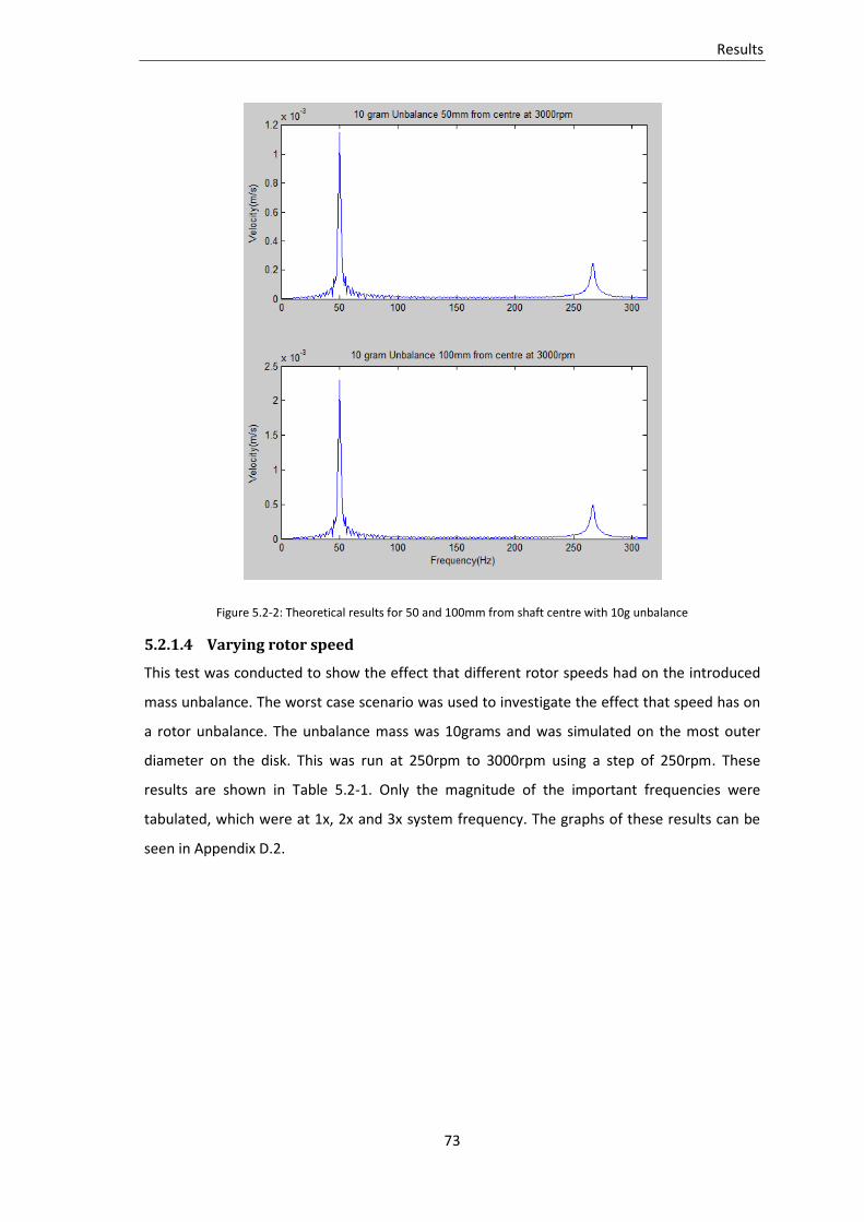
73
Results
Figure 5.2-2: Theoretical results for 50 and 100mm from shaft centre with 10g unbalance
5.2.1.4 Varying rotor speed
This test was conducted to show the effect that different rotor speeds had on the introduced
mass unbalance. The worst case scenario was used to investigate the effect that speed has on
a rotor unbalance. The unbalance mass was 10grams and was simulated on the most outer
diameter on the disk. This was run at 250rpm to 3000rpm using a step of 250rpm. These
results are shown in Table 5.2-1. Only the magnitude of the important frequencies were
tabulated, which were at 1x, 2x and 3x system frequency. The graphs of these results can be
seen in Appendix D.2.
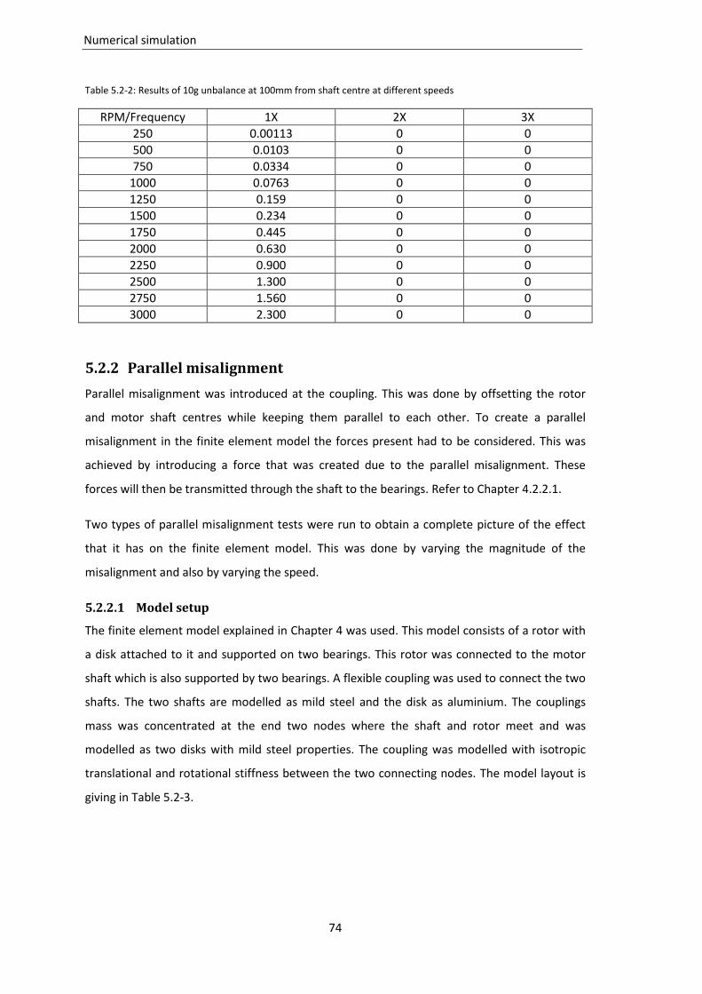
74
Numerical simulation
Table 5.2-2: Results of 10g unbalance at 100mm from shaft centre at different speeds
RPM/Frequency 1X 2X 3X
250 0.00113 0 0
500 0.0103 0 0
750 0.0334 0 0
1000 0.0763 0 0
1250 0.159 0 0
1500 0.234 0 0
1750 0.445 0 0
2000 0.630 0 0
2250 0.900 0 0
2500 1.300 0 0
2750 1.560 0 0
3000 2.300 0 0
5.2.2 Parallel misalignment
Parallel misalignment was introduced at the coupling. This was done by offsetting the rotor
and motor shaft centres while keeping them parallel to each other. To create a parallel
misalignment in the finite element model the forces present had to be considered. This was
achieved by introducing a force that was created due to the parallel misalignment. These
forces will then be transmitted through the shaft to the bearings. Refer to Chapter 4.2.2.1.
Two types of parallel misalignment tests were run to obtain a complete picture of the effect
that it has on the finite element model. This was done by varying the magnitude of the
misalignment and also by varying the speed.
5.2.2.1 Model setup
The finite element model explained in Chapter 4 was used. This model consists of a rotor with
a disk attached to it and supported on two bearings. This rotor was connected to the motor
shaft which is also supported by two bearings. A flexible coupling was used to connect the two
shafts. The two shafts are modelled as mild steel and the disk as aluminium. The couplings
mass was concentrated at the end two nodes where the shaft and rotor meet and was
modelled as two disks with mild steel properties. The coupling was modelled with isotropic
translational and rotational stiffness between the two connecting nodes. The model layout is
giving in Table 5.2-3.

75
Results
Table 5.2-3: Full model layout
Nodes 1 2 3 4 5 6 7 8 9 10 11 12
Shaft diameter(mm) 40 50 40 30 30 30 40 50 50 50 40
Components B D B C B D B
Disk Diameter(mm) 100 230
Stiffness N/m
Damping Ns/m 80 80 80 80
Parallel misalignment was modelled by considering the geometry of the coupling. The coupling
has three jaws on each side with a rubber element insert. Each leg of this insert was modelled
as a linear spring. Parallel misalignment was introduced by changing the length of the springs.
As the coupling rotated the length of the springs varied and a vibration was introduced in the
system. The full derivation can be seen in Chapter 4.2.2.1.
5.2.2.2 Varying parallel displacement
This test was conducted to show the effect that parallel misalignment had on the finite
element model when the magnitude was varied. The magnitudes used were the same as those
used in the experimental tests. These were 0.3, 0.6 and 0.9mm parallel misalignment at the
coupling. Figure 5.2-3 shows the frequency plots of a constant rotor speed with three different
parallel misalignments.

76
Numerical simulation
Figure 5.2-3: Theoretical results for 0.3, 0.6 and 0.9mm parallel misalignment
5.2.2.3 Varying rotor speed
This test was done to show the effect that different rotor speeds had on the introduced
parallel misalignment. The maximum parallel misalignment of 0.9mm, from the experimental
test, was used. This test was run at 250rpm to 3000rpm using a step of 250rpm. These results
are shown in Table 5.2-2. Only the magnitude of the important frequencies was tabulated
which were at 1x, 2x and 3x system frequency. The graphs of these results can be seen in
Appendix D.3.
Table 5.2-4: Results of 0.9mm parallel misalignment at different speeds
RPM/Frequency 1X 2X 3X
250 0.017 0.035 0.046
500 0.038 0.068 0.095
750 0.052 0.090 0.153
1000 0.065 0.130 0.210
1250 0.082 0.170 0.250
1500 0.090 0.205 0.275
1750 0.120 0.235 0.360
2000 0.126 0.260 0.440
2250 0.145 0.275 0.500
2500 0.162 0.338 0.520
2750 0.160 0.390 0.640
3000 0.215 0.442 0.770

77
Results
5.2.3 Angular misalignment
Angular misalignment was introduced at the coupling. This was achieved by creating an angle
between the rotor and motor shaft. To create angular misalignment in the finite element
model the forces present had to be considered. This was achieved by introducing a force that
was created due to the angular misalignment. These forces will then be transmitted through
the shaft to the bearings.
Two types of angular misalignment tests were run to obtain a complete picture of the effect
that it had on the finite element model. This was done by varying the magnitude of the
misalignment and also by varying the speed.
5.2.3.1 Model setup
The finite element model explained in Chapter 4 was used. This model consists of a rotor with
a disk attached to it and supported by two bearings. This rotor was connected to the motor
shaft which was also supported by two bearings. A flexible coupling was used to connect the
two shafts. The two shafts were modelled as mild steel and the disk as aluminium. The
couplings mass was concentrated at the end two nodes were the shaft and rotor meet and
modelled as two disks with mild steel properties. The coupling was modelled with isotropic
translational and rotational stiffness between the two connecting nodes. Model layout is
exactly the same as the one for parallel misalignment and can be seen in Table 5.2-3.
Angular misalignment was modelled by considering the geometry of the coupling. The
coupling has three jaws on each side with a rubber element insert. Each leg of this insert was
modelled as a linear spring. Angular misalignment was introduced by changing the length of
the springs. As the coupling rotated the length of the springs varied and a vibration was
introduced into the system. The full derivation can be seen in Chapter 4.2.2.2.
5.2.3.2 Varying angle
This test was done to show the effect that angular misalignment had on the finite element
model when the magnitude of the angle was varied. The angles used were the same as those
used in the experimental tests. These were 0.5, 1 and 2 degrees angular misalignment at the
coupling. Figure 5.2-4 shows the frequency plots of a constant rotor speed with three different
parallel misalignments.

78
Numerical simulation
Figure 5.2-4: Theoretical results for 0.5, 1 and 2 degrees misalignment
5.2.3.3 Varying rotor speed
This test was conducted to show the effect that different rotor speeds have on the introduced
angular misalignment. The maximum angular misalignment, of 2 degrees, from the
experimental test was used. This test was run at 250rpm to 3000rpm using a step of 250rpm.
These results are shown in Table 5.2-3. Only the magnitude of the important frequencies was
tabulated, which are at 1x, 2x and 3x system frequency. The graphs of these results can be
seen in Appendix D.4.
Table 5.2-5: Results of 2 degrees misalignment at different speeds
RPM/Frequency 1X 2X 3X
250 0.023 0.112 0.085
500 0.042 0.220 0.166
750 0.060 0.295 0.260
1000 0.067 0.427 0.355
1250 0.085 0.568 0.427
1500 0.089 0.699 0.466
1750 0.119 0.796 0.618
2000 0.125 0.868 0.758
2250 0.136 0.949 0.867
2500 0.159 1.158 0.905
2750 0.165 1.36 1.149
3000 0.205 1.525 1.405
79
Results
5.3 Chapter summary
This chapter looked at the results obtained from the experimental test rig as well as the finite
element model. The three tests shown are unbalance at the rotor disk, parallel and angular
misalignment. The test rig setup and finite element model of each test were also explained in
detail along with the different variations of the faults that were introduced into the system.
The frequency response of each test was also provided either as a graph or in table form. The
next chapter explained what these results meant and how it was used to identify faults.

80
Chapter summary

81
Chapter 6
Discussion of results The results obtained from the finite element model and the experimental test rig are shown in
Chapter 5. These results show the behaviour of the system when certain faults are introduced
to a rotor bearing test rig. The results will be discussed in more detail in this Chapter, giving an
insight on how to identify the fault present in the system. This will be done for the numerical
as well as for the experimental results then finally the two will be compared.
6.1 Experimental results
For the experimental setup a base line had to be established first before any testing could be
done. A base line was achieved by aligning and balancing the system to the best tolerances
possible. The base line result will then show the 1x system frequency and its harmonics with
the remaining misalignment and unbalance that is present. This result was used to identify any
change in the system.
Results for the base line were captured at rotating speeds of 250rpm to 3000rpm in 250rpm
steps. This revealed that as the rotational speed increase so does the 1x, 2x and 3x system
frequencies. It was also seen that the 1x system frequency was dominant to the others with a
maximum value of 0.682mm/s. The maximum value is not at 3000rpm but at 1750rpm this
was due to the fact that the rotor bearing test rig goes through resonance at roughly 1750rpm.

82
Experimental results
These results are tabulated in Chapter 5, Table 5.1-1. It was noticed that the 2x and 3x peaks
also increases at the same rotating speed of 1750rpm but not as much as the 1x.
The first test was unbalance of the rotor disk. The unbalance was introduced by bolting a
weight to the rotor disk. Unbalance was tested in three different ways. These were varying the
unbalance mass, varying the position of the unbalance mass and by varying the speed. The
disk was initially balanced to the given tolerance and the unbalance mass was checked using a
scale with capability of measuring up to an accuracy of 1mg. The two unbalance weights used
were a 5 and 10gram weight. The disk also had predrilled holes where the weight bolts on to.
The holes were drilled using a CNC to ensure accuracy of the position of the unbalance mass.
For all tests explained here on the rotational speed will be 3000rpm. Results with other
rotational speeds have similar outcomes and can be seen in Chapter 5 and Appendix C
All mass unbalance tests showed one prominent characteristic a major increase in the 1x
system frequency with the 2x and 3x staying roughly the same as the base line values. Varying
the mass unbalance and varying the unbalance position has similar effect on the system. This
was due to the fact that mass and distance is directly proportional to the force created by the
mass unbalance. This meant that if the unbalance mass was doubled so was the force in the
system. This means that an imbalance of 5g at 100mm from the shaft centre has exactly the
same response as an imbalance of 10g at 50mm from the shaft centre axis.
This effect was noted in Chapter 5 in Figure 5.1-2 and 5.1-3 where the 5g imbalance at 100mm
had a 1.223mm/s response and the 10g imbalance at 50mm had a 1.243mm/s response. This
result showed that only the imbalance force can be identified in the system and not the
position and magnitude. This result was still useful in identifying if there was an imbalance in
the system and will also show the severity because it shows the force present in the system.
The flexible coupling was used to introduce the parallel and angular misalignment into the
system. This was achieved by either offsetting the centre lines of the two shafts or creating an
angle between then. The first parallel and angular misalignment tests were done just below
the couplings rated limit of misalignment. It was seen that this had little effect on the system
frequencies. The coupling rubber element used was still new and was able to dampen the
misalignment effectively. For this reason the flexible coupling was misaligned passed its
maximum misalignment limit. This was done to overcome the dampening of the coupling so
that the effect of misalignment can become apparent in the frequency plots.

83
Discussion of results
The first parallel misalignment was done at 0.3mm offset followed by a 0.6 and 0.9mm offset.
This showed an increase in the 2x and 3x system frequencies as the offset increased.
Comparing base line to the 0.3, 0.6 and 0.9mm parallel misalignment tests it was seen that
there was little to no change in the 1x system frequency. The base line test had a 1x system
frequency peak at 0.1927mm/s, while the 0.3mm offset had a 0.2149mm/s peak, 0.6mm had a
0.1495mm/s peak and 0.9mm had a 0.293mm/s peak.
The 2x and 3x system frequencies had a much bigger increase and definitively showed the
parallel misalignment that was present. The base line 2x and 3x peaks were 0.1267 and
0.0576mm/s respectively. The 0.9mm parallel misalignment showed an increase of 126.5% at
the 2x and a 2095% increase at 3x system frequency from base line. The same trend was noted
at the other two tests with the 3x dominating. These results can be seen in Figure 5.1-4.
Angular misalignment tests were done at 0.5, 1 and 2 degrees. This showed an increase in the
1x and 2x system frequencies as the angle increased. Comparing base line to the 0.5, 1 and 2
degrees angular misalignment tests it was seen that there was little to no change in the 3x
system frequency. The base line test had a 3x system frequency peak at 0.0576mm/s, while
0.5 degrees had a 0.0646mm/s peak, 1 degree had a 0.0191mm/s peak and 2 degrees had a
0.0721mm/s peak.
The 1x and 2x system frequencies has a much bigger increase and definitively shows the
angular misalignment that was present. The base line 1x and 2x peaks were 0.1927 and
0.1267mm/s respectively. The 2 degree angular misalignment showed an increase of 93.2% at
1x and 193.9% at 2x system frequency from base line. The same trend was noted for the other
two tests with the 2x dominating. These results can be seen in Figure 5.1-5.
6.2 Numerical simulation
For numerical simulation, there was no need for a base line result. This was due to the fact
that the simulation was noise free and the fault introduced will be the only disturbance in the
system. The finite element model was derived to simulate the test rig as closely as possible.
The shaft was given a stiffness that corresponds to the mild steel that was used in the test rig.
The mass of the system was calculated using the densities of the material present, mild steel
for the shaft and aluminium for the disk.
The bearings on the test rig had a non-linear effect on the system and are difficult to simulate.
The bearings for the finite element model were linearized to simplify the simulation and

84
Numerical simulation
reduce computation time. A generalised value was chosen for the stiffness and damping of the
bearings as this may vary considerably from bearing to bearing. These values will only affect
the peak values and not the frequency at which the peaks occur. A few trial simulations were
run to find stiffness and damping values that produced results that were interpretable for this
research. The best stiffness value was found to be around 7x10⁶N/m while the damping was
80Ns/m.
For all test explained here on the rotational speed will be 3000rpm. Results with other
rotational speeds have similar outcomes and can be seen in Chapter 5 and Appendix D.
The first simulated test was unbalance in the rotor. This was achieved by adding a
concentrated mass to the disk at a certain distance from the shaft centre. This was done by
creating a forcing function that had to be added to the finite element model. This forcing
function will include the concentrated mass to be added, the distance from the centre and the
frequency at which the system will run at. See Chapter 4.2.1.
It was seen that this forcing function introduced a disturbance in the 1x system frequency with
no effect to the 2x and 3x system frequencies. Varying the mass unbalance and varying the
unbalance position had similar effect on the system. This is due to the fact that mass and
distance is directly proportional to the force created by the mass unbalance and was seen in
the forcing function. This meant that an imbalance of 5g at 100mm from the shaft centre had
exactly the same response as an imbalance of 10g at 50mm from the shaft centre axis.
This effect was noted in Chapter 5 in Figure 5.2-1 and 5.2-2 where the 5g imbalance at 100mm
had a 1.1504mm/s response and the 10g imbalance at 50mm was exactly the same with also a
1.1504mm/s response. This result showed that only the imbalance force can be identified in
the system and not the position and magnitude. This result showed that unbalance can be
definitely identified by an increase of the 1x system frequency. The magnitude of the peak at
the 1x system frequency can also be used to determine the severity as this is directly related
to the force present in the system.
Misalignment was introduced in to the finite element model by simulating the forces that was
present at the coupling. First the behaviour of the coupling had to be explained. The coupling
model used in this research was derived by Nelson and Crandall [21]. This model was
explained in Chapter 4.1.2.4. This model can be used for any flexible coupling. This research
considered a flexible jaw coupling. The difference can only be seen in the forcing function
where the rubber element was added to the coupling model. The misalignment was expressed

85
Discussion of results
as a function of the forces created by the compression or shear in the rubber element. These
forces are also dependent on the frequency of the system.
The first parallel misalignment was done at 0.3mm offset followed by a 0.6 and 0.9mm offset.
This showed dominating peaks in the 2x and 3x system frequencies as the offset increased.
There was also a small 1x system frequency peak present. With the parallel misalignment the
3x system frequency was always the biggest dominating frequency. Increasing the parallel
misalignment from 0.3mm to 0.6mm increased the 3x system frequency peak from
0.2585mm/s to 0.5165mm/s. A similar effect was seen when the parallel misalignment was
taken to 0.9mm.
This shows that the severity of parallel misalignment can be determined by taking note of the
3x system frequency. There was a direct correlation between the parallel misalignment and
the peak values of the dominating system frequencies. These results can be seen in Figure 5.2-
3.
The angular misalignment was done at 0.5, 1 and 2 degrees. This showed dominating peaks in
the 2x and 3x system frequencies as the angle increased. There was also a small 1x system
frequency peak present. This was similar to the parallel misalignment but in this case the 2x
system frequency was the biggest dominating frequency and not the 3x. Increasing the angular
misalignment from 0.5 to 1 degree increased the 2x system frequency peak from 1.017mm/s
to 1.271mm/s. A similar effect was seen when the angular misalignment was taken to 2
degrees.
This showed that the severity of angular misalignment can be determined by taking note of
the 2x system frequency. There was a direct correlation between the angular misalignment
and the peak values of the dominating system frequencies. These results can be seen in Figure
5.2-4.
6.3 Comparing numerical to simulation
For comparing purposes the rotor bearing test rig and the finite element model was kept
identical where possible while also considering computational time. Sacrifices had to be made
in the finite element model at the bearings and the coupling. These two components were
nonlinear and had to be linearized to minimize computational time. For this reason there was
a difference in the peak values between the experimental and numerical simulation but no
effect on the system frequency and its harmonics.

86
Chapter summary
Looking at the unbalance results it was seen that both the experimental and numerical results
showed an increase in the 1x system frequency. This can be defined as an indicator that
unbalance was present in the system. Comparing the peak values it was seen that they have
the same trend but not the same magnitude. This was caused by two external factors, one
being from the experimental test rig and the other from the finite element model. The first
was due to the fact that the experimental test rig can never be perfectly balanced and aligned.
This was why a base line test was done to identify the noise and the presence of unwanted
misalignment and unbalance. The second factor was in the finite element model where the
bearings were linearized.
Parallel misalignment tests done for experimental and numerical simulation showed similar
results. These were a dominating 2x and 3x system frequency response, with the 3x being the
larger of the two. Comparing the peak values of the experimental and simulation it was seen
that there was a difference. This was due to the same reason as for the unbalance along with
the linearized coupling model. These results gave a clear indication of what effect parallel
misalignment had on a rotor bearing system.
Angular misalignment tests done for experimental and numerical simulation also showed
similar results. These were a dominating 2x and 3x system frequency response with the 2x
being the larger of the two. Comparing the peak values of the experimental and simulation it
was seen that there was a difference. This was due to the same reason as for the parallel
misalignment. These results gave a clear indication of what effect angular misalignment has on
a rotor bearing system.
6.4 Chapter summary
This chapter took the results obtained from the rotor bearing test rig and the numerical
simulation and explained it in more detail. Firstly the experimental tests were looked at and
what effect unbalance, parallel and angular misalignment had on the system. The same was
done for the numerical simulation. Lastly the two were compared and reasons were given why
certain errors occurred. The next Chapter concludes this research and proposes possible
future research.

87
Chapter 7
Conclusion and recommendations for future research This chapter will be used to tie up all aspect of the dissertation and give a picture of what was
done in order to achieve the objectives that were stated in Chapter 1. A brief description of
work that ties up with this research is also given. This also includes future research.
7.1 Research conclusion
Condition monitoring of a rotor bearing system was researched. It was seen that this is a very
big field in itself. It was therefore decided to focus only on the vibration aspect of condition
monitoring. This decision was made on the grounds that this is the most common method of
condition monitoring used in industry. Vibration monitoring can be used to identify various
types of faults that are present in rotor bearing systems. It was then chosen to look at the
three most common faults that usually occur in industry which are unbalance, parallel
misalignment and angular misalignment.
An experimental test rig was built that can run up to 3000rpm. This speed was important as
this ensured that the test rig went through its first resonant frequency. The test rig was also
built in such a way that a controllable unbalance and misalignment could be introduced into
the system. The test rig was also successfully isolated, ensuring that the noise from

88
Research conclusion
neighbouring systems was minimized as much as possible. The final design of the test rig
consists of a rotor supported by two roller bearings with a disk at the middle. The rotor is
driven by a three phase electric motor that is controlled by a variable speed drive. The rotor
and motor shaft is connected using a flexible three jaw coupling. The disk has six holes
predrilled where the unbalance weights could be bolted. The motor base was equipped with
setting screws that ensured that the desired misalignment could be achieved.
This exact setup was then modelled using Lagrange method and finite element analysis.
Energy methods were used to describe the behaviour of each component in the rotor bearing
system and then assembled into a global system. The coupling and bearings in the rotor
bearing system was linearized to reduce computation time. The bearing stiffness and damping
values were taken from available literature and adapted to correlate with this research. The
rotor was also modelled with a constant rotational speed.
The simulated faults were also successfully derived using first principals and by extending an
existing coupling model to fit in with this research. The faults were successfully introduced into
the finite element model and useful results were obtained. Even though the finite element
model was simplified to a certain extend it still gave results that corresponded to the results
obtained from the rotor bearing test rig.
A definite trend was noted when the results were quantified. It was seen that unbalance has
an increase in the 1x system frequency with little to no effect to the 2x and 3x frequencies.
This was seen in the experimental and simulation results. It was also noted that as the rotor
speed increase so does the response in the frequency plots. The peak value is a function of the
square of the speed. This means that the response increase exponentially as the speed
increases.
Parallel misalignment was successfully identified by an increase in the 2x and 3x system
frequencies with the 3x being the larger of the two. This was seen in the experimental and
simulated results. It was also noted that as the rotor speed increased the first three system
frequencies also increased. The same effect was note when parallel misalignment was
increased. Increasing both rotor speed and magnitude of the fault caused a linear increase in
the peak values except when the rotor was close to its resonant frequency. In this case the
peak values increased significantly.
Angular misalignment was also successfully identified by an increase in the 2x and 3x system
frequencies, with the 2x system frequency being the larger of the two. This was seen in the
89
Conclusion and recommendations for future research
experimental and simulation results. Exactly the same behaviour was observed in angular
misalignment as in parallel misalignment with respect to increasing the rotor speed and
increasing the degree of misalignment. When the system went through resonant frequency it
also caused the peak values to increase significantly.
The results obtained from the experimental test rig were successfully compared to the
numerically simulated results. Three major factors were identified that caused the results to
differ slightly from each other. This was due to the linearization of the bearings and the
coupling model and also the fact that the experimental test rig can never be perfectly
balanced and aligned. These factors only contributed to the difference in the peak values of
the system frequencies. The peak values are important in determining the severity of the fault
but a residual technique can eliminate these errors.
7.2 Future research
Only a subsection of condition monitoring was considered in this research. This was vibration
monitoring of rotor bearing systems and more specifically looking only at three faults. These
were unbalance, parallel misalignment and angular misalignment. For future research this can
be expanded to look at other faults that could also affect a rotor bearing system like rotor
cracks, rotor bends and clearance at journals. The basic finite element model has already been
set up and only needs to be modified to accommodate these faults. The test rig is constructed
and can be modified easily.

90
Future research

91
References [1] K. Mechefske, 2005. Machine condition monitoring and fault diagnostics. In C.W. de
Silva Vibration and shock hand book. Boca Raton: CRC Press Taylor & Francis Group.
Ch 25.
[2] S. Wichtendahl, 2003. Cost Effective Predictive Maintenance Solutions [online].
(Updated 21 Jan 2010) Available at: http://www.wilcoxon.com/knowdesk/
Cost%20Effective%20PdM%20Solutions.pdf [accessed 15 April 2010]
[3] C.W de Silva, 2005. Vibration design and control. In C.W. de Silva Vibration and Shock
Hand Book. Boca Raton: CRC Press Taylor & Francis Group. Ch 32.
[4] L. Cveticanin, 2005. Free vibration of a Jeffcott rotor with pure cubic non-linear elastic
property of the shaft. Mechanism and Machine Theory, 40, p.1330-1344.
[5] H. Samarasekera, 2005. Vibration in Rotating Machinery. In C.W. de Silva Vibration and
Shock Hand Book. Boca Raton: CRC Press Taylor & Francis Group. Ch 34.
[6] A. W. Lees, M. I. Friswell, 1997. The evaluation of rotor unbalance in flexibly mounted
machines. Journal of Sound and Vibration, 208, p.671-683.
[7] S. Edwards, A. W. Lees, M. I. Friswell, 2000. Experimental identification of excitation
and support parameters of a flexible rotor-bearing-foundation system from a single
run-down. Journal of Sound and Vibration, 232, p.963-992.
[8] Kr. Jalan, A. R. Mohanty, 2009. Model based fault diagnosis of a rotor-bearing system
for misalignment and unbalance under steady-state conditions. Journal of Sound and
Vibration, 327, p.604-622.

92
References
[9] R. Platz, R. Market, 2001. Fault models for on-line identification of malfunctions in
rotor systems. Transaction of Fourth International Conference on Acoustical and
vibration Surveillance , p.435-446.
[10] J. K. Sinha, A. W. Lees and M. I. Friswell, 2004. Estimating unbalance and
misalignment of a flexible rotating machine from a single run-down. Journal of Sound
and Vibration, p.272, 967-989.
[11] M. Xu, R. D. Marangoni, 1994. Vibration analysis of a motor-flexible coupling-rotor
system subject to misalignment and unbalance. Part 1: theoretical model and analysis.
Journal of Sound and Vibration, 176, p.663-679.
[12] C. B. Gibbons, 1976. Coupling misalignment. In proceedings of the 5th
Turbomachinery Symposium, Gas Turbine Laboratories, Texas A&M University.
[13] P. Arumugam, S. Swarnamani and B. S Prabhu, 1995. Effects of coupling misalignment
on the vibration characteristics of a two stage turbine rotor. ASME Design Engineering
Technical Conferences, 84, p.1049-1054.
[14] A. S. Sekhar and B. S. Prabhu, 1995. Effects of coupling misalignment on vibrations of
rotating machinery. Journal of Sound and Vibration, 185, p.655-671.
[15] Kr. Jalan, A. R. Mohanty, 2009. Model based fault diagnosis of a rotor-bearing system
for misalignment and unbalance under steady-state conditions. Journal of Sound and
Vibration, 327, p.604-622.
[16] Y. S. Lee and C. W. Lee, 1999. Modelling and Vibration analysis of misaligned rotor-
ball bearing systems. Journal of Sound and Vibration, 224, p.17-32.
[17] D. L. Dewell, L. D. Mitchell, 1984. Detection of misalignment disk coupling using
spectrum analysis. Journal of Vibration, Acoustics, Stress and Reliability in Design, 106,
p.9-16.
[18] S. Prabhakar, A. S. Sekhar, A. R. Mohanty, 2002. Crack versus coupling misalignment in
a transient rotor system. Journal of Sound and Vibration, 256, p.773-786.
[19] A. W. Lees, 2007. Misalignment in rigidly coupled rotors. Journal of Sound and
Vibration, 305, p.261-271.
[20] E. Kramer 1993. Dynamics of Rotors and Foundations. 1st ed. Springer-Verlag.
[21] H.D. Nelson, S.H. Crandall, 1992. Analytic prediction of rotordynamic response. In F.F.
Ehrich Handbook of Rotor Dynamics. The University of Michigan: McGraw-Hill. Ch 2.
[22] A. T. Tadeo, K. L. Cavalca, 2003. A Comparison of Flexible Coupling Models for
Updating in Rotating Machinery Response. Journal of the Brazilian Society of
Mechanical Sciences and Engineering, 25, p.235-246.

93
Appendix A
Rotor bearing test rig components This Chapter gives the specifications of all the components used in the rotor bearing test rig. It
also shows a detailed shaft design that was done and assembly drawings that were used to
manufacture the rotor bearing test rig.
A.1 Motor details
The motor was the first component that was sized for the rotor bearing test rig. it was seen
that a 0.55Kw motor was sufficient for the test rig. It was not too big and could easily be
moved around and it was also big enough to achieve the desired tolerances in the
misalignment. The motor specifications is given by Figure A.1-1.
Figure A.1-1: Motor specifications
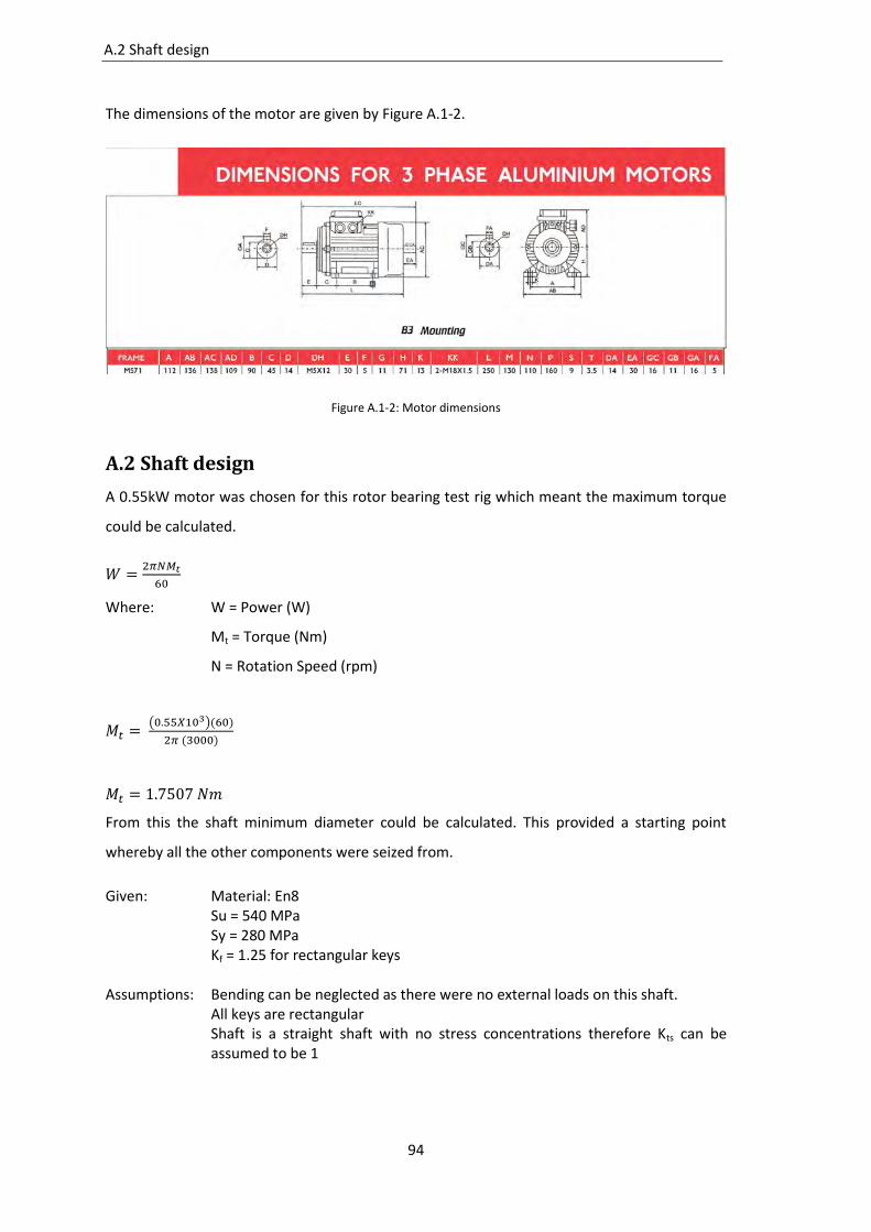
94
A.2 Shaft design
The dimensions of the motor are given by Figure A.1-2.
Figure A.1-2: Motor dimensions
A.2 Shaft design
A 0.55kW motor was chosen for this rotor bearing test rig which meant the maximum torque
could be calculated.
Where: W = Power (W)
Mt = Torque (Nm)
N = Rotation Speed (rpm)
( )( )
( )
From this the shaft minimum diameter could be calculated. This provided a starting point
whereby all the other components were seized from.
Given: Material: En8 Su = 540 MPa Sy = 280 MPa Kf = 1.25 for rectangular keys
Assumptions: Bending can be neglected as there were no external loads on this shaft.
All keys are rectangular Shaft is a straight shaft with no stress concentrations therefore Kts can be assumed to be 1

95
A.3 Rotex flexible coupling
Substituting known values into equation the minimum allowable diameter of the shaft can be
calculated.
[
8(
)
.
/ 9
]
Where: M = bending moment (Nm) Kt = concentration factor for bending Kts= concentration factor for torsion Su = Ultimate tensile strength Sy = Yield strength
[ ( )
{( ) .
/
}
]
It was seen that the smallest part of the shaft was at the coupling. The coupling connects the
motor to the shaft. It was seen that the motor shaft had a diameter of 15mm. In order to keep
the coupling interchangeable the minimum shaft diameter was also made 15mm. this also
gave the shaft a safety factor of 3.
A.3 Rotex flexible coupling
The coupling chosen was a rotex flexible 19 coupling with a 92 shore A spider. This coupling
was ideal as it was capable of a wide range of misalignment. The coupling specifications are
given in Figure A.3-1.

96
A.3 Rotex flexible coupling
Figure A.3-1: Coupling specifications
The dimensions of the coupling are given by Figure A.3-2.
Figure A.3-2: Coupling dimensions

97
A.4 Bearing dimensions
A.4 Bearing dimensions
The minimum shaft diameter was made 15mm and this was at the coupling position. The next
component on the shaft is the bearing a standard step size of 10 mm was used to determine
the bearing diameter. Using catalogues it was seen that there was a bearing with a 25mm
diameter bore. This was the UCP205D1 bearing from NTN. Figure A.4-1 gives the dimensions
of the bearing. The same bearings were used to support the shaft on both sides.
Figure A.4-1: Bearing dimensions
A.5 Test rig drawings
Drawing 1: Full assembly
Drawing 2: Vibration rig top
Drawing 3: Vibration rig stand assembly
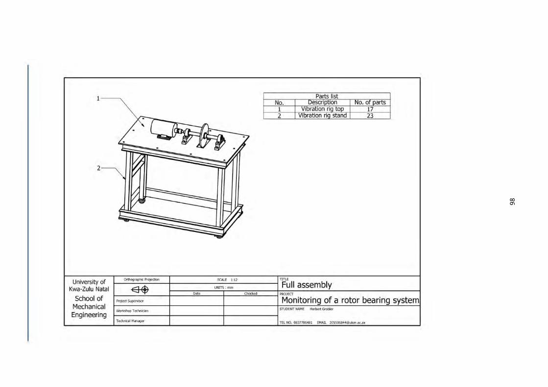
98
1------. Parts list No. Descnptron No. of parts
2
University of Kwa-Zulu Natal
School of Mechanical Engineering
1 Vibration rig top 17 2 Vibration riq stand 23
Orthographic Proje<tion SCALE 1:12 TITlE
~ UNITS:mm Full assembly I -.;:;:;:::rw Date O>ed<ed PROJECT
ProJect SopeN!sor Monitoring of a rotor bearing system Workshop Technician STUOENT NAME Herbert Grobles
Te<J>nitill ~1"""90'" TEL NO. 01!37786481 EMAn. [email protected]

99
University of Kwa-Zulu Natal
SChool of Mechanical Engineering
'-3
'----------5
No. 1 2
3
4
5 6 7 8 9
10
11 12 13 14 15
DescriPtion Motor
Adapter plate Bearing housing
bottom Bearmg housmg
top Pillow block
Roller bearing Coupling 14mm Couolinq 15mm Couphng spider Disk boss with
crub screw Disk
Plain bearing Shaft Key
Base plate
1 Orthographic Proje<tion SCALE 1:8 nnE
~ UNITS : mm Vibration rig top I -.::::;;:r-w oate Oledted PROJECT
Amount 1 1
1
1
1 1 1 1 1
2
1 1 1 2 1
Proj<CtSuPM1sor I Monitoring of a rotor bearing system Workshop Technician STUOENT NAME Herbert Groble<
Te<hnk;ol ~lonogor TEL NO. 0837786481 EMA1l [email protected]

10
0
No.
1 3----.... \ 2
3
4 5
6---... c ~-- /// / /r-Y../-1 6 7 8
4
'----8 '-----7
University of Kwa-Zulu Natal
Orthographic Proje<tion SCALE 1:11 TITlE
~ uNITS:mm Vibration rig stand assembly I -.;:;:;:::rw Date O>ed<ed PROJECT
Amount
2
2
2
4 1 4 4 4
School of Mechanical Engineering
ProJect SopeN!sor Monitoring of a rotor bearing system Workshop Technician STUOENT NAME Herbert Grobles
Te<J>nitill ~1"""90'" TEL NO. 01!37786481 EMAn. [email protected]
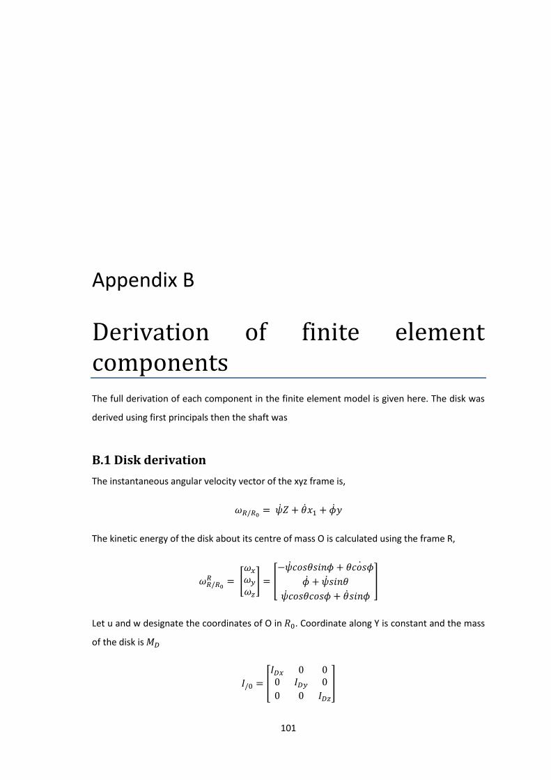
101
Appendix B
Derivation of finite element components The full derivation of each component in the finite element model is given here. The disk was
derived using first principals then the shaft was
B.1 Disk derivation
The instantaneous angular velocity vector of the xyz frame is,
The kinetic energy of the disk about its centre of mass O is calculated using the frame R,
[
] [
]
Let u and w designate the coordinates of O in . Coordinate along Y is constant and the mass
of the disk is
[
]

102
B.2 Shaft derivation
Kinetic energy of a disk
( )
(
)
Disk is symmetric ( )
Angles are small ( )
Angular velocity is constant so
( )
(
)
( )
= const (represents the energy of the disk rotating at )
= gyroscopic effect (coriolis)
At a given node the rotor has four degrees of freedom: two displacement u and w, and two
slopes about the X and Z axes which are
* + {
}
Application of Lagrange gives:
(
)
[
] [
]
[
] [
]
B.2 Shaft derivation
Kinetic energy:
The general formulation of the kinetic energy of the shaft comes from an extension of the disk
equation. For an element of length L, the expression for the kinetic energy is:
∫ ( )
∫ ( )
∫
The relations between displacement and slopes are:

103
B.2 Shaft derivation
And the nodal displacement vector is
* +
{
}
where
* + {
}
* + {
}
The finite element is built from
( )
( )
( ) and ( ) are the typical displacement functions of the beam in bending
( ) [
]
( ) [
]

104
B.2 Shaft derivation
Substituting u and w into K.E. gives
∫ ,
-
∫ 6
7
∫ 6
7
Substitute ( ) and ( ) then integrate:
and = classical mass matrices
and = secondary effect of rotating inertia
= gyroscopic effect
Application of Lagrange gives
(
)
, -* + , -* +
where
[
]
[
]

105
B.2 Shaft derivation
[
]
Strain energy:
(
)
(
)
= linear terms
= non-linear terms
Strain energy is:
∫
Then
∫ (
)
The symmetry of the beam cross-section with respect to x and z gives:
∫
Also is second order and is neglected
∫ ∫ 4
5
∫ ∫ [ 4
5
4
5
]

106
B.2 Shaft derivation
Due to symmetry
Diametral cross-section of inertia
∫
∫
Then
∫ [ 4
5
4
5
]
If the shaft is subjected to a constant axial force , then there is a second contribution to the
strain energy
∫
( )
=0 (due to symmetry)
∫ 6(
)
(
)
7
The combined strain energy is then
∫ [ 4
5
4
5
]
∫ 6(
)
(
)
7
It is necessary to express the strain energy as a function of u and w – components of
displacement in (To avoid periodic terms explicitly function of time)

107
B.2 Shaft derivation
∫ [ 4
5
4
5
]
∫ 6(
)
(
)
7
Shaft is symmetric
∫ [4
5
4
5
]
∫ 6(
)
(
)
7
Recall:
( )
( )
Then
∫ 6
7
∫ 6
7
After integration
Taking into account the shear effect
Where
( )
poisson’s ratio
reduced area of cross-section
influence of the shear effect

108
B.3 Bearing derivation
classical stiffness matrix
axial force
Application of Lagrange gives
Where
( )
[
( ) ( )
( ) ( )
( ) ( )
( ) ( ) ]
If a=0 then is a classical stiffness matrix of a beam in bending
[
]
B.3 Bearing derivation
The virtual work of the forces acting on the shaft can be written as
Or

109
B.4 Matlab code used for simulation
The main characteristics link forces and displacements, and the influence of slopes and
bending moments is neglected here
= 0 so,
[
] [
] [
] [
] [
]
B.4 Matlab code used for simulation
Main code used to call other functions and assemble the global matrices:
clc
clear all
global iter
iter = 0;
count = 4;
M_matrix = zeros(48,48);
Gc_matrix = zeros(48,48);
Cb_matrix = zeros(48,48);
Ks_matrix = zeros(48,48);
Kb_matrix = zeros(48,48);
Kc_matrix = zeros(48,48);
%element 1, node 1 and node 2
%shaft has a diameter of 30mm and lenght of 75mm
D1 = 0.030; %Diameter of shaft element 1
L1 = 0.090; %Length of element 1
Ms1 = shaft_mass(D1,L1);
Gc1 = shaft_gyro(D1,L1);
Ks1 = shaft_stiffness(D1,L1);
for i = 1:8
for j = 1:8
M_matrix(i,j) = M_matrix(i,j) + Ms1(i,j);
Gc_matrix(i,j) = Gc_matrix(i,j) + Gc1(i,j);
Ks_matrix(i,j) = Ks_matrix(i,j) + Ks1(i,j);
end
end
%element 2, node 2 and node 3
%shaft has a diameter of 30mm and lenght of 75mm
D2 = 0.030; %Diameter of shaft element 2
L2 = 0.090; %Length of element 2
Ms2 = shaft_mass(D2,L2);
Gc2 = shaft_gyro(D2,L2);
Ks2 = shaft_stiffness(D2,L2);

110
B.4 Matlab code used for simulation
for i = 1:8
for j = 1:8
M_matrix(count + i,count + j) = M_matrix(count + i,count + j) + Ms2(i,j);
Gc_matrix(count + i,count + j) = Gc_matrix(count + i,count + j) + Gc2(i,j);
Ks_matrix(count + i,count + j) = Ks_matrix(count + i,count + j) + Ks2(i,j);
end
end
count = count + 4;
%element 3, node 3 and node 4
D3 = 0.030; %Diameter of shaft element 3
L3 = 0.040; %Length of element 3
Ms3 = shaft_mass(D3,L3);
Gc3 = shaft_gyro(D3,L3);
Ks3 = shaft_stiffness(D3,L3);
for i = 1:8
for j = 1:8
M_matrix(count + i,count + j) = M_matrix(count + i,count + j) + Ms3(i,j);
Gc_matrix(count + i,count + j) = Gc_matrix(count + i,count + j) + Gc3(i,j);
Ks_matrix(count + i,count + j) = Ks_matrix(count + i,count + j) + Ks3(i,j);
end
end
count = count + 4;
%element 4, node 4 and node 5
%shaft has a diameter of 30mm and lenght of 75mm
D4 = 0.030; %Diameter of shaft element 4
L4 = 0.020; %Length of element 4
Ms4 = shaft_mass(D4,L4);
Gc4 = shaft_gyro(D4,L4);
Ks4 = shaft_stiffness(D4,L4);
for i = 1:8
for j = 1:8
M_matrix(count + i,count + j) = M_matrix(count + i,count + j) + Ms4(i,j);
Gc_matrix(count + i,count + j) = Gc_matrix(count + i,count + j) + Gc4(i,j);
Ks_matrix(count + i,count + j) = Ks_matrix(count + i,count + j) + Ks4(i,j);
end
end
count = count + 4;
%element 5, node 5 and node 6
%dummy element only has the stiffness of the coupling
Mc5 = coupling_mass;
Gcoup5 = coupling_gyro;
Cc5 = coupling_damping;
Kc5 = coupling_stiffness;
for i = 1:8
for j = 1:8
M_matrix(count + i,count + j) = M_matrix(count + i,count + j) + Mc5(i,j);
Gc_matrix(count + i,count + j) = Gc_matrix(count + i,count + j) + Gcoup5(i,j);
Kc_matrix(count + i,count + j) = Kc_matrix(count + i,count + j) + Kc5(i,j);
end
end
count = count + 4;
%element 6, node 6 and node 7
%shaft has a diameter of 30mm and lenght of 75mm
D6 = 0.030; %Diameter of shaft element 6
L6 = 0.020; %Length of element 6
Ms6 = shaft_mass(D6,L6);
Gc6 = shaft_gyro(D6,L6);
Ks6 = shaft_stiffness(D6,L6);

111
B.4 Matlab code used for simulation
for i = 1:8
for j = 1:8
M_matrix(count + i,count + j) = M_matrix(count + i,count + j) + Ms6(i,j);
Gc_matrix(count + i,count + j) = Gc_matrix(count + i,count + j) + Gc6(i,j);
Ks_matrix(count + i,count + j) = Ks_matrix(count + i,count + j) + Ks6(i,j);
end
end
count = count + 4;
%element 7, node 7 and node 8
%shaft has a diameter of 30mm and lenght of 75mm
D7 = 0.030; %Diameter of shaft element 7
L7 = 0.040; %Length of element 7
Ms7 = shaft_mass(D7,L7);
Gc7 = shaft_gyro(D7,L7);
Ks7 = shaft_stiffness(D7,L7);
for i = 1:8
for j = 1:8
M_matrix(count + i,count + j) = M_matrix(count + i,count + j) + Ms7(i,j);
Gc_matrix(count + i,count + j) = Gc_matrix(count + i,count + j) + Gc7(i,j);
Ks_matrix(count + i,count + j) = Ks_matrix(count + i,count + j) + Ks7(i,j);
end
end
count = count + 4;
%element 8, node 8 and node 9
%shaft has a diameter of 30mm and lenght of 75mm
D8 = 0.030; %Diameter of shaft element 8
L8 = 0.090; %Length of element 8
Ms8 = shaft_mass(D8,L8);
Gc8 = shaft_gyro(D8,L8);
Ks8 = shaft_stiffness(D8,L8);
for i = 1:8
for j = 1:8
M_matrix(count + i,count + j) = M_matrix(count + i,count + j) + Ms8(i,j);
Gc_matrix(count + i,count + j) = Gc_matrix(count + i,count + j) + Gc8(i,j);
Ks_matrix(count + i,count + j) = Ks_matrix(count + i,count + j) + Ks8(i,j);
end
end
count = count + 4;
%element 9, node 9 and node 10
%shaft has a diameter of 30mm and lenght of 75mm
D9 = 0.030; %Diameter of shaft element 9
L9 = 0.090; %Length of element 9
Ms9 = shaft_mass(D9,L9);
Gc9 = shaft_gyro(D9,L9);
Ks9 = shaft_stiffness(D9,L9);
for i = 1:8
for j = 1:8
M_matrix(count + i,count + j) = M_matrix(count + i,count + j) + Ms9(i,j);
Gc_matrix(count + i,count + j) = Gc_matrix(count + i,count + j) + Gc9(i,j);
Ks_matrix(count + i,count + j) = Ks_matrix(count + i,count + j) + Ks9(i,j);
end
end
count = count + 4;
%element 10, node 10 and node 11
%shaft has a diameter of 30mm and lenght of 75mm
D10 = 0.030; %Diameter of shaft element 10
L10 = 0.090; %Length of element 10
Ms10 = shaft_mass(D10,L10);
Gc10 = shaft_gyro(D10,L10);
Ks10 = shaft_stiffness(D10,L10);

112
B.4 Matlab code used for simulation
for i = 1:8
for j = 1:8
M_matrix(count + i,count + j) = M_matrix(count + i,count + j) + Ms10(i,j);
Gc_matrix(count + i,count + j) = Gc_matrix(count + i,count + j) + Gc10(i,j);
Ks_matrix(count + i,count + j) = Ks_matrix(count + i,count + j) + Ks10(i,j);
end
end
count = count + 4;
%element 11, node 11 and node 12
%shaft has a diameter of 30mm and lenght of 75mm
D11 = 0.030; %Diameter of shaft element 11
L11 = 0.090; %Length of element 11
Ms11 = shaft_mass(D11,L11);
Gc11 = shaft_gyro(D11,L11);
Ks11 = shaft_stiffness(D11,L11);
for i = 1:8
for j = 1:8
M_matrix(count + i,count + j) = M_matrix(count + i,count + j) + Ms11(i,j);
Gc_matrix(count + i,count + j) = Gc_matrix(count + i,count + j) + Gc11(i,j);
Ks_matrix(count + i,count + j) = Ks_matrix(count + i,count + j) + Ks11(i,j);
end
end
count = count + 4;
%disk, at node 10
%disk has diameter of 230mm
Md10 = disk_mass;
Gd10 = disk_gyro;
for i = 1:4
for j = 1:4
M_matrix(36 + i,36 + j) = M_matrix(36 + i,36 + j) + Md10(i,j);
Gc_matrix(36 + i,36 + j) = Gc_matrix(36 + i,36 + j) + Gd10(i,j);
end
end
%Bearing at node 1
Kb1 = bearing_stiffness;
Cb1 = bearing_damping;
for i = 1:4
for j = 1:4
Kb_matrix(i,j) = Kb_matrix(i,j) + Kb1(i,j);
Cb_matrix(i,j) = Cb_matrix(i,j) + Cb1(i,j);
end
end
%Bearing at node 3
Kb3 = bearing_stiffness;
Cb3 = bearing_damping;
for i = 1:4
for j = 1:4
Kb_matrix(8 + i,8 + j) = Kb_matrix(8 + i,8 + j) + Kb3(i,j);
Cb_matrix(8 + i,8 + j) = Cb_matrix(8 + i,8 + j) + Cb3(i,j);
end
end
%Bearing at node 8
Kb8 = bearing_stiffness;
Cb8 = bearing_damping;
for i = 1:4
for j = 1:4
Kb_matrix(28 + i,28 + j) = Kb_matrix(28 + i,28 + j) + Kb8(i,j);
Cb_matrix(28 + i,28 + j) = Cb_matrix(28 + i,28 + j) + Cb8(i,j);
end
end

113
B.4 Matlab code used for simulation
%Bearing at node 12
Kb12 = bearing_stiffness;
Cb12 = bearing_damping;
for i = 1:4
for j = 1:4
Kb_matrix(44 + i,44 + j) = Kb_matrix(44 + i,44 + j) + Kb12(i,j);
Cb_matrix(44 + i,44 + j) = Cb_matrix(44 + i,44 + j) + Cb12(i,j);
end
end
%solving Lagrange equation using ode
q = zeros(48,1);
qdot = zeros(48,1);
p0 = [q; qdot];
ts = linspace(0,0.5,5000);
rpm = 2000;
omg = (2*pi*rpm)/60;
K = Ks_matrix + Kb_matrix +Kc_matrix;
C = Cb_matrix - omg*Gc_matrix;
[t,p] = ode45('lagrange',ts,p0,[],M_matrix,C,K);
function pdot = lagrange(t,p,flag,m_matrix,c,k)
global iter
iter = iter + 1
k1 = 1*10^4;
r = 0.05; %coupling raduis
del_y = 0.001; %coupling misalignment
alpha_1 = 0;
alpha_2 = 2*pi/3;
alpha_3 = 4*pi/3;
beta_1 = pi/3;
beta_2 = pi;
beta_3 = 5*pi/3;
rpm = 3000; %rotor 1 speed - constant
omg = (2*pi*rpm)/60;
rho = 7850; %density of shaft
D = 0.04; %diameter of shaft
I = (pi*D^4)/64;
L = 0.075;
%Parallel misalignment
x1 = r*cos(beta_1 + omg*t) - r*cos(alpha_1 + omg*t);
y1 = r*sin(beta_1 + omg*t) - r*sin(alpha_1 + omg*t) + del_y;
x2 = r*cos(beta_2 + omg*t) - r*cos(alpha_2 + omg*t);
y2 = r*sin(beta_2 + omg*t) - r*sin(alpha_2 + omg*t) + del_y;
x3 = r*cos(beta_3 + omg*t) - r*cos(alpha_3 + omg*t);
y3 = r*sin(beta_3 + omg*t) - r*sin(alpha_3 + omg*t) + del_y;
del_L1 = sqrt((x1)^2 + (y1)^2) - r;
del_L2 = sqrt((x2)^2 + (y2)^2) - r;
del_L3 = sqrt((x3)^2 + (y3)^2) - r;
e1 = atan(y1/x1);
e2 = atan(y2/x2);
e3 = atan(y3/x3);
Fx = del_L1*k1*cos(e1) + del_L2*k1*cos(e2) + del_L3*k1*cos(e3);
Fy = del_L1*k1*sin(e1) + del_L2*k1*sin(e2) + del_L3*k1*sin(e3);
% angular misalignment
YL1 = r*sin(alpha_1 + omg*t);
YR1 = r*sin(beta_1 + omg*t);
YL2 = r*sin(alpha_2 + omg*t);
YR2 = r*sin(beta_2 + omg*t);
YL3 = r*sin(alpha_3 + omg*t);

114
B.4 Matlab code used for simulation
YR3 = r*sin(beta_3 + omg*t);
yL1 = r-YL1;
yR1 = r-YR1;
yL2 = r-YL2;
yR2 = r-YR2;
yL3 = r-YL3;
yR3 = r-YR3;
thetaL1 = atan(yL1/xs);
thetaR1 = atan(yR1/xs);
thetaL2 = atan(yL2/xs);
thetaR2 = atan(yR2/xs);
thetaL3 = atan(yL3/xs);
thetaR3 = atan(yR3/xs);
delL1 = xs*tan(thetaL1);
delR1 = xs*tan(thetaR1);
delL2 = xs*tan(thetaL2);
delR2 = xs*tan(thetaR2);
delL3 = xs*tan(thetaL3);
delR3 = xs*tan(thetaR3);
E1 = atan(YR1 - YL1/x1);
E2 = atan(YR2 - YL2/x2);
E3 = atan(YR3 - YL3/x3);
FLy = k(delL1*sin(E1) + delL2*sin(E2) + delL3*sin(E3));
FLx = k(delL1*cos(E1) + delL2*cos(E2) + delL3*cos(E3));
FRy = k(delR1*sin(E1) + delR2*sin(E2) + delR3*sin(E3));
FRx = k(delR1*cos(E1) + delR2*cos(E2) + delR3*cos(E3));
%unbalance of disk
m = 0.005; %mass in kg
e = 0.100; %distance in meters
B = zeros(48,1);
%Unbalance
B(37,1) = (omg^2)*m*e*sin(omg*t);
B(38,1) = (omg^2)*m*e*cos(omg*t);
%Misalignment
B(17,1) = Fx; or B(17,1) = FLx + FRx;
B(18,1) = Fy; B(18,1) = FLy + FRy;
B(21,1) = -Fx; B(21,1) = -(FLx + FRx);
B(22,1) = -Fy; B(22,1) = -(FLy + FRy);
A = [zeros(48) eye(48); -inv(m_matrix)*k -inv(m_matrix)*c];
f = inv(m_matrix)*B;
pdot = A*p +[zeros(48,1); f];
function Md = disk_mass
AL_rho = 2800; %Mass Density of aluminum kg/m^3
Dd = 0.230; %Diameter of the disk
Sd = (pi*Dd^2)/4; %Cross-sectional area
Ld = 0.012; %Length of disk
Vd = Sd*Ld; %Volume of disk
md = AL_rho*Vd; %Mass of disk kg
Idx = (md*Dd^2)/16; %Moment of inertia for disk
Md = [md 0 0 0;
0 md 0 0;
0 0 Idx 0;
0 0 0 Idx];

115
B.4 Matlab code used for simulation
function Dd = disk_gyro
AL_rho = 2800; %Density of aluminum kg/m^3
Dd = 0.230; %Diameter of the disk m
Sd = (pi*Dd^2)/4; %Cross-sectional area m^2
Ld = 0.012; %Length of disk m
Vd = Sd*Ld; %Volume of disk m^3
md = AL_rho*Vd; %Mass of disk kg
Idy = (md*Dd^2)/8; %Moment of inertia for disk kg*m^2
%rpm = 3000; %revolutions per minute
%omg = (2*pi*rpm)/60; %rad/s
Dd = [0 0 0 0;
0 0 0 0;
0 0 0 Idy;
0 0 -Idy 0];
function Ms = shaft_mass(D,L)
rho = 7850; %Mass Density of mild steel kg/m^3
S = (pi*D^2)/4; %Cross-sectional area m^2
I = (pi*D^4)/64; %Moment of inertia m^4
X = rho*S*L/420; %kg
Y = rho*I/(30*L); %kg
M1 = X*[156 0 0 -22*L 54 0 0 13*L;
0 156 22*L 0 0 54 -13*L 0;
0 22*L 4*L^2 0 0 13*L -3*L^2 0;
-22*L 0 0 4*L^2 -13*L 0 0 -3*L^2;
54 0 0 -13*L 156 0 0 22*L;
0 54 13*L 0 0 156 -22*L 0;
0 -13*L -3*L^2 0 0 -22*L 4*L^2 0;
13*L 0 0 -3*L^2 22*L 0 0 4*L^2];
M2 = Y*[36 0 0 -3*L -36 0 0 -3*L;
0 36 3*L 0 0 -36 3*L 0;
0 3*L 4*L^2 0 0 -3*L -L^2 0;
-3*L 0 0 4*L^2 3*L 0 0 -L^2;
-36 0 0 3*L 36 0 0 3*L;
0 -36 -3*L 0 0 36 -3*L 0;
0 3*L -L^2 0 0 -3*L 4*L^2 0;
-3*L 0 0 -L^2 3*L 0 0 4*L^2];
Ms = M1 + M2;
function Ds = shaft_gyro(D,L)
rho = 7850; %Mass Density of mild steel kg/m^3
I = (pi*D^4)/64; %Moment of inertia m^4
%rpm = 3000; %revolutions per minute
%omg = (2*pi*rpm)/60; %rad/s
X = rho*I/(15*L); %kg*rad/s
Ds = X*[0 -36 -3*L 0 0 36 -3*L 0;
36 0 0 -3*L -36 0 0 -3*L;
3*L 0 0 -4*L^2 -3*L 0 0 L^2;
0 3*L 4*L^2 0 0 -3*L -L^2 0;
0 36 3*L 0 0 -36 3*L 0;
-36 0 0 3*L 36 0 0 3*L;
3*L 0 0 L^2 -3*L 0 0 -4*L^2;
0 3*L -L^2 0 0 -3*L 4*L^2 0];

116
B.4 Matlab code used for simulation
function Ks = shaft_stiffness(D,L)
E = 210e9; %N/m^2
I = (pi*D^4)/64; %Moment of inertia
X = E*I/L^3; %N/m
Ks = X*[12 0 0 -6*L -12 0 0 -6*L;
0 12 6*L 0 0 -12 6*L 0;
0 6*L 4*L^2 0 0 -6*L 2*L^2 0;
-6*L 0 0 4*L^2 6*L 0 0 2*L^2;
-12 0 0 6*L 12 0 0 6*L;
0 -12 -6*L 0 0 12 -6*L 0;
0 6*L 2*L^2 0 0 -6*L 4*L^2 0;
-6*L 0 0 2*L^2 6*L 0 0 4*L^2];
function Kb = bearing_stiffness
kxx = 7*10^8; %Stiffness N/m
kzz = 7*10^8;
kxz = 0;
kzx = 0;
Kb = [kxx 0 0 0;
0 kzz 0 0;
0 0 0 0;
0 0 0 0];
function Db = bearing_damping
cxx = 8; %Ns/m
czz = 8;
cxz = 0;
czx = 0;
Db = [cxx 0 0 0;
0 czz 0 0;
0 0 0 0;
0 0 0 0];
function Mc = coupling_mass
rho = 7800; %Mass Density kg/m^3
Dd = 0.050; %Diameter of the disk
Sd = (pi*Dd^2)/4; %Cross-sectional area
Ld = 0.030; %Length of disk
Vd = Sd*Ld; %Volume of disk
mc1 = rho*Vd; %Mass of disk kg
Ic1 = (mc1*Dd^2)/16; %Moment of inertia for disk
mc2 = mc1;
Ic2 = Ic1;
Mc = [mc1 0 0 0 0 0 0 0;
0 mc1 0 0 0 0 0 0;
0 0 Ic1 0 0 0 0 0;
0 0 0 Ic1 0 0 0 0;
0 0 0 0 mc2 0 0 0;
0 0 0 0 0 mc2 0 0;
0 0 0 0 0 0 Ic2 0;
0 0 0 0 0 0 0 Ic2];

117
B.4 Matlab code used for simulation
function Gcoup = coupling_gyro
rho = 7800; %Density kg/m^3
Dd = 0.050; %Diameter of the disk m
Sd = (pi*Dd^2)/4; %Cross-sectional area m^2
Ld = 0.030; %Length of disk m
Vd = Sd*Ld; %Volume of disk m^3
md = rho*Vd; %Mass of disk kg
Ic1 = (md*Dd^2)/8; %Moment of inertia for disk kg*m^2
%rpm = 3000; %revolutions per minute
%omg = (2*pi*rpm)/60; %rad/s
Ic2 = Ic1;
Gcoup = [0 0 0 0 0 0 0 0;
0 0 0 0 0 0 0 0;
0 0 0 Ic1 0 0 0 0;
0 0 -Ic1 0 0 0 0 0;
0 0 0 0 0 0 0 0;
0 0 0 0 0 0 0 0;
0 0 0 0 0 0 0 Ic2;
0 0 0 0 0 0 -Ic1 0];
function Kc = coupling_stiffness
Kt = 1*10^3;
Kr = 1*10^1;
Kc = [Kt 0 0 0 -Kt 0 0 0;
0 Kt 0 0 0 -Kt 0 0;
0 0 Kr 0 0 0 -Kr 0;
0 0 0 Kr 0 0 0 -Kr;
-Kt 0 0 0 Kt 0 0 0;
0 -Kt 0 0 0 Kt 0 0;
0 0 -Kt 0 0 0 Kr 0;
0 0 0 -Kr 0 0 0 Kr];
%simplified code that was used for the unbalance simulation
clc
clear all
global iter
iter = 0;
count = 4;
M_matrix = zeros(20,20);
D_matrix = zeros(20,20);
K_matrix = zeros(20,20);
%element 1, node 1 and node 2
%shaft has a diameter of 30mm and lenght of 75mm
D1 = 0.030; %Diameter of shaft element 1
L1 = 0.075; %Length of element 1
Ms1 = shaft_mass(D1,L1);
Ds1 = shaft_gyro(D1,L1);
Ks1 = shaft_stiffness(D1,L1);
for i = 1:8
for j = 1:8
M_matrix(i,j) = M_matrix(i,j) + Ms1(i,j);
D_matrix(i,j) = D_matrix(i,j) + Ds1(i,j);
K_matrix(i,j) = K_matrix(i,j) + Ks1(i,j);
end
end
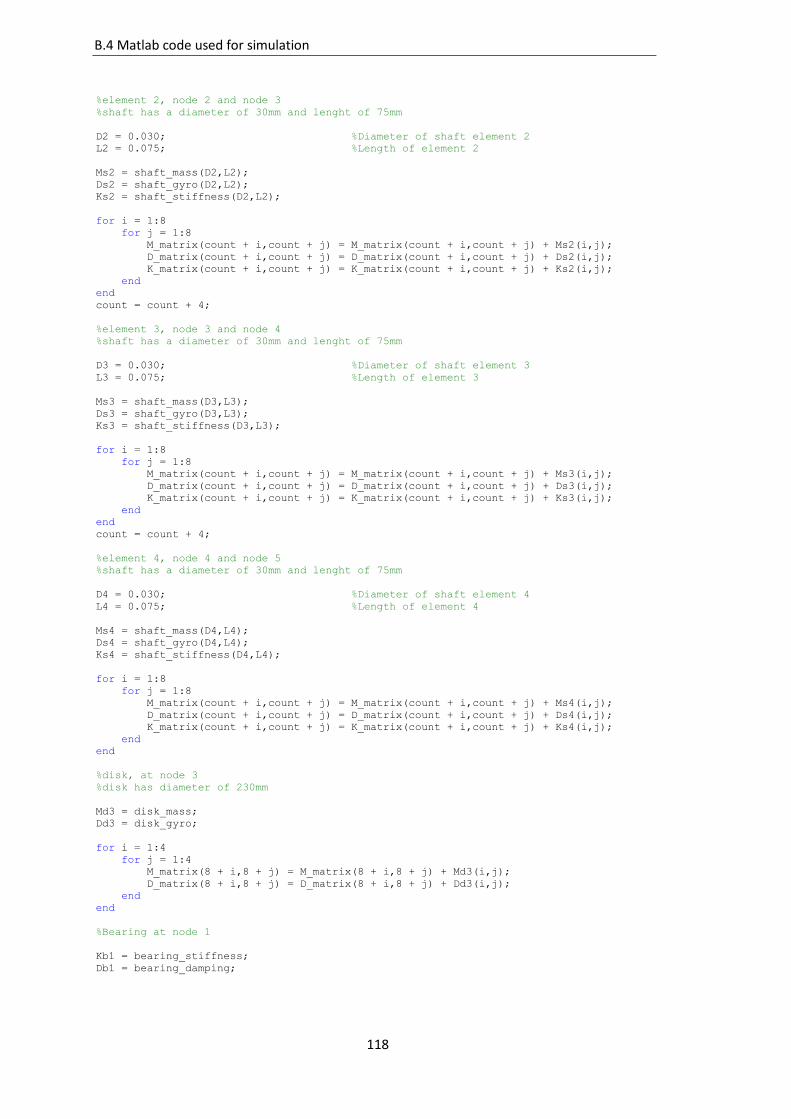
118
B.4 Matlab code used for simulation
%element 2, node 2 and node 3
%shaft has a diameter of 30mm and lenght of 75mm
D2 = 0.030; %Diameter of shaft element 2
L2 = 0.075; %Length of element 2
Ms2 = shaft_mass(D2,L2);
Ds2 = shaft_gyro(D2,L2);
Ks2 = shaft_stiffness(D2,L2);
for i = 1:8
for j = 1:8
M_matrix(count + i,count + j) = M_matrix(count + i,count + j) + Ms2(i,j);
D_matrix(count + i,count + j) = D_matrix(count + i,count + j) + Ds2(i,j);
K_matrix(count + i,count + j) = K_matrix(count + i,count + j) + Ks2(i,j);
end
end
count = count + 4;
%element 3, node 3 and node 4
%shaft has a diameter of 30mm and lenght of 75mm
D3 = 0.030; %Diameter of shaft element 3
L3 = 0.075; %Length of element 3
Ms3 = shaft_mass(D3,L3);
Ds3 = shaft_gyro(D3,L3);
Ks3 = shaft_stiffness(D3,L3);
for i = 1:8
for j = 1:8
M_matrix(count + i,count + j) = M_matrix(count + i,count + j) + Ms3(i,j);
D_matrix(count + i,count + j) = D_matrix(count + i,count + j) + Ds3(i,j);
K_matrix(count + i,count + j) = K_matrix(count + i,count + j) + Ks3(i,j);
end
end
count = count + 4;
%element 4, node 4 and node 5
%shaft has a diameter of 30mm and lenght of 75mm
D4 = 0.030; %Diameter of shaft element 4
L4 = 0.075; %Length of element 4
Ms4 = shaft_mass(D4,L4);
Ds4 = shaft_gyro(D4,L4);
Ks4 = shaft_stiffness(D4,L4);
for i = 1:8
for j = 1:8
M_matrix(count + i,count + j) = M_matrix(count + i,count + j) + Ms4(i,j);
D_matrix(count + i,count + j) = D_matrix(count + i,count + j) + Ds4(i,j);
K_matrix(count + i,count + j) = K_matrix(count + i,count + j) + Ks4(i,j);
end
end
%disk, at node 3
%disk has diameter of 230mm
Md3 = disk_mass;
Dd3 = disk_gyro;
for i = 1:4
for j = 1:4
M_matrix(8 + i,8 + j) = M_matrix(8 + i,8 + j) + Md3(i,j);
D_matrix(8 + i,8 + j) = D_matrix(8 + i,8 + j) + Dd3(i,j);
end
end
%Bearing at node 1
Kb1 = bearing_stiffness;
Db1 = bearing_damping;

119
B.4 Matlab code used for simulation
for i = 1:4
for j = 1:4
K_matrix(i,j) = K_matrix(i,j) + Kb1(i,j);
D_matrix(i,j) = D_matrix(i,j) + Db1(i,j);
end
end
%Bearing at node 5
Kb5 = bearing_stiffness;
Db5 = bearing_damping;
for i = 1:4
for j = 1:4
K_matrix(16 + i,16 + j) = K_matrix(16 + i,16 + j) + Kb5(i,j);
D_matrix(16 + i,16 + j) = D_matrix(16 + i,16 + j) + Db5(i,j);
end
end
q = zeros(20,1);
qdot = zeros(20,1);
%q(1,1) = 0.1;
p0 = [q; qdot];
ts = linspace(0,0.5,5000);
[t,p] = ode45('lagrange',ts,p0,[],M_matrix,D_matrix,K_matrix);

120
B.4 Matlab code used for simulation

121
Appendix C
Experimental test rig results
C.1 Baseline alignment report
Figure C.1-1: Base line alignment report
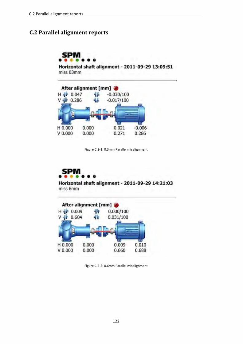
122
C.2 Parallel alignment reports
C.2 Parallel alignment reports
Figure C.2-1: 0.3mm Parallel misalignment
Figure C.2-2: 0.6mm Parallel misalignment

123
C.3 Angular alignment reports
Figure C.2-3: 1mm Parallel misalignment
C.3 Angular alignment reports
Figure C.3-1: 0.5 Degrees angular misalignment

124
C.3 Angular alignment reports
Figure C.3-2: 1 Degree angular misalignment
Figure C.3-3: 2 Degrees angular misalignment

125
C.4 Baseline varying speed graphs
C.4 Baseline varying speed graphs
Figure C.4-1: Base line varying speed graphs 250RPM - 1500RPM
50
0 . OOORPM: 1000 RPM (2011/09/27 1314 53) ·001 .01 Base Line 1 mm/s l;i AOA
0.45 0.40 0.35 0.30 0.25 0.20 0.15
·001 .07 Base Line mm/s ei AOA RPM (2011/09/271349:25) · 1250RPM: 1250
0.45 0.40 0.35 0.30 0.25 0.20 0.15
50
0 (2011/09/271 3:53:54) mm/s eil AOA ·001.08 Base Line 1500 . RPM 1500RPM 0.45 0.40 0.35 0.30 0.25
100
100

126
C.4 Baseline varying speed graphs
Figure C.4-2: Base line varying speed graphs 1750RPM - 3000RPM
0.4
0.2
0.4
0.2
0.4
0.2
. 1750RPM 1750RPM (2011/09/27 13:55:29) Ml\·001.09 Base L01e
50
Ml\·001 .02 Base Line RPM (2011/09/27 13:1 9:13) . 2000R PM: 2000
50
Ml\·001.10 Baseline 2250RPM (2011/09/2713:59:36) · 2250RPM
50
0 . 500RPM: 2500RPM 001 11 Base Lne 2 ....... MO,. . mm/s - (2011 109/27 14:01 :31)
0.6
0.4
0.2
50
Ml\·001.12 Base Lne 27 . 50RPM: 2750RPM ( 2011109/271 4:05:41)
0.4
0.2
50
0 . 3000 RPM (2011 109/27 1323:30) . 3000RPM. AI'A·001.03 Base Lne mm/s ~
0.6
0.4
0.2
50
100 150
100 150
100 150
100 200 Hz
100
100 150

127
C.5 Unbalance graphs
C.5 Unbalance graphs
Figure C.5-1: 10g unbalance 100mm from centre for 250RPM – 1500RPM
3.5
3.0
2.5
2.0
1.5
50 0
0 (2011/09/1513:13:49) PM: 10g10 mm -002.05 Unbalance 15Cffi mm/s ~ AOA
3.5
3.0
2.5
2.0
1.5
1.0
0.5
50
100
100

128
C.5 Unbalance graphs
Figure C.5-2: 10g unbalance 100mm from centre for 1750RPM – 3000RPM
Ml>.-002.06 Unbalance 175 . (2011 /09/28 12:05 59) ORPM· 10g 100mm
50
(2011 /09/28 12:07 20) 0 PM· 10g 100mm Ml>.-002.07 Unbalance 2250R . mm/s l.:iJ
2.0
1.5
1.0
50
Ml>.-002.08 Unbalance 250 (201 1/09/2812:11 :56) ORPM: 10g 100mm
50
/09/28 12 15:12) 0 2750RPM: 10g 1 OOmm (201 1 Ml>.-002.09 Unbalance mm/s ~ 3.0
1.5
1.0
0.5
50
0 0 RPM: 10g 100mm Ml>.-002.03 Unbalance 300 mm/s e;, 3.0
(2011 /09/28 11 :50: 12)
100 150 200 Hz
100 150 200 Hz
100 150
100 150
200 Hz i:::1.5 :=:d::::==:::::t::::::::=:~ '" ,. 100
0.5
50

129
C.6 Parallel misalignment graphs
C.6 Parallel misalignment graphs
Figure C.6-1: 0.9mm Parallel misalignment for 250RPM – 1500RPM
1.2
1.0
0.8
0.6
0.2
0 9mm 12011/10/2410:56:10) . 1250RPM ParaDel . ~ AOA003.07 Misa~gnment . mm/s ...-
0.4L~~~~~Hz 1.2
1.0
0.8
0.6
0.4
0.2
50 100
0 I O 9 (201111 0/24 10:54:31 l 1500RPM· Parane · rml <'h AI>A·003.08 Misa~gnment · mm/s -..
1.2
1.0
0.8
0.6 0.4 0.2
50 100

130
C.6 Parallel misalignment graphs
Figure C6-2: 0.9mm Parallel misalignment for 1750RPM – 3000RPM
1.0
0.8
0.6
0.4
0.2
(2011 /10/24 10:53:081 ---;::7;;:::50;;;:R>DPM: Pa~allel 0.9mm AAA·003.09 Misalignment 1
50 100
0 . 2000RPM: Pa>allel 0.9mm ( AAA·003.02 Misalignment mm/s ~ 2011 /10/24 10:51:411
1.2
1.0
0.8
0.6
0.4
0.2
50 100
0 . 250RPM: Pa~allel 0.9mm ( mm/s ~ AAA· · 003 1 0 M isahgnment 2 201 1/10/2410:50:151
1.2
1.0
0.8
0.6
0.4
0.2
50 (2011/ 10/241 0:48:521 . 2500RPM: Pa>allel 0.9mm Misaignment
100
50 100
0 . ?50RPM: Pa>allel 0.9mm I .,., AAA·003.12 Misaignment 2 mmls ..- 201 1/ 10/241 0:45:431
0.8
0.6
0.4
1.0
0.8
0.6
0.4
0.2
50
. JOOORPM: Pa>allel 0.9mm AAA·003.03 Misaignment
50
100
(201 1/ 1 0/24 10:20:011
100
I 150 200 Hz
150
150
150 200 Hz
150 200 Hz
150

131
C.7 Angular misalignment graphs
C.7 Angular misalignment graphs
Figure C.7-1: 2 Degrees angular misalignment for 250RPM – 1500RPM
0.25
0.20
0.15
0.10
0.25
0.20
0.15
010
0.05
50
0 I 2(2011 /10/211 2:30:41 ) 5CffiPM· Angu ar """ AM-003. OS Misalignment 1 . mmls ..-
0.25
0.20
0.1 5
0.10
50

132
C.7 Angular misalignment graphs
Figure C.7-2: 2 Degrees angular misalignment for 1750RPM – 3000RPM
0.4
0.4
0.2
0.4
0.2
A¥.·003.09 Misalignment 1 . 750R PM Angular 2 (201 1/10/2112:29:111
50
Misalignment 2 (2011 /10/2112:23:391 500RPM: Angular 2
50
2 (2011 /10/2112:21:031 0 . 2750RPM: Angular AAA-003.12 Misalignment mm/s eil
0.4
0.2
50
2 (2011 /10/ 2112:17:381 0 . 3000RPM: Angular AAA-003.03 Misalignment mm/s e;r,
0.4
0.2
I 100 150
100 150
100 150 200 Hz
100 150
100 150 200 Hz
150

133
Appendix D
Numerical simulation results
D.1 Comparison graph of finite element models
Figure D.1-1: Comparison of full and simplified finite element model

134
D.2 Unbalance graphs
D.2 Unbalance graphs
Figure D.2-1: 10g unbalance 100mm from centre for 250RPM – 1500RPM

135
D.2 Unbalance graphs
Figure D.2-2: 10g unbalance 100mm from centre for 1750RPM – 3000RPM

136
D.3 Parallel misalignment graphs
D.3 Parallel misalignment graphs
Figure D.3-1: 0.9mm Parallel misalignment for 250RPM – 1500RPM

137
D.3 Parallel misalignment graphs
Figure D.3-2: 0.9mm Parallel misalignment for 1750RPM – 3000RPM

138
D.4 Angular misalignment graphs
D.4 Angular misalignment graphs
Figure D.4-1: 2 Degrees angular misalignment for 250RPM – 1500RPM

139
D.4 Angular misalignment graphs
Figure D.4-2: 2 Degrees angular misalignment for 1750RPM – 3000RPM