conﬁguration and evaluation of the wrf model for the study

Configuration and Evaluation of the WRF Model for the Study of HawaiianRegional Climate

CHUNXI ZHANG, YUQING WANG, AXEL LAUER, AND KEVIN HAMILTON

International Pacific Research Center, and Department of Meteorology, School of Ocean and

Earth Science and Technology, University of Hawaii at Manoa, Honolulu, Hawaii

(Manuscript received 26 September 2011, in final form 30 March 2012)

ABSTRACT

The Weather Research and Forecasting (WRF) model V3.3 has been configured for the Hawaiian Islands

as a regional climate model for the region (HRCM). This paper documents the model configuration and

presents a preliminary evaluation based on a continuous 1-yr simulation forced by observed boundary con-

ditions with 3-km horizontal grid spacing in the inner nested domain. The simulated vertical structure of the

temperature and humidity are compared with twice-daily radiosonde observations at two stations. Generally

the trade wind inversion (TWI) height and occurrence days are well represented. The simulation over the

islands is compared with observations from nine surface climatological stations and a dense network of

precipitation stations. The model simulation has generally small biases in the simulated surface temperature,

relative humidity, and wind speed. The model realistically simulated the magnitude and geographical dis-

tribution of the mean rainfall over the Hawaiian Islands. In addition, the model simulation reproduced

reasonably well the individual heavy rainfall events as seen from the time series of pentad mean rainfall

averaged over island scales. Also the model reproduced the geographical variation of the mean diurnal

rainfall cycle even though the observed diurnal cycle displays quite different features over different islands.

Comparison with results obtained using the land surface dataset from the official release of the WRF model

confirmed that the newly implemented land surface dataset generally improved the simulation of surface

variables. These results demonstrate that the WRF can be a useful tool for dynamical downscaling of regional

climate over the Hawaiian Islands.

1. Introduction

The main Hawaiian Islands stretch between 18.98 and

22.28N in the central North Pacific and are affected

year-round by the prevalent trade winds. The regional

climate over the Hawaiian Islands can be characterized

by two seasons: ‘‘summer’’ between May and October

and ‘‘winter’’ between October and April (http://www.

prh.noaa.gov/hnl/pages/climate_summary.php). Despite

being in a region of large-scale mean descent, rainfall

over the Hawaiian Islands is frequent and abundant

principally because of the strong interaction between the

orography and prevailing trade winds (Schroeder 1993).

The trade wind–induced rainfall along the windward

sides of the mountains is the most significant contributor

to the statewide rainfall (Lyons 1982). In winter, the trade

winds may be interrupted for days or weeks by the

invasion of fronts or migratory cyclones from the

midlatitude and by Kona storms (Kona storms are ex-

tratropical cyclones usually formed in winter resulting in

westerly winds, ‘‘Kona’’ in Hawaiian). Therefore, winter

in Hawaii is the season of more frequent heavy rain-

storms (Schroeder et al. 1977). In summer, tropical dis-

turbances originating in the intertropical convergence

zone (ITCZ) can influence the Hawaiian Islands and

occasionally cause severe precipitation events (Chu and

Clark 1999). Sometimes, the local sea breeze can also

bring heavy showers to the Hawaiian Islands, especially

over the Big Island (Schroeder 1981; Chen and Nash

1994). It is a challenge for regional models to simulate all

of these different synoptic systems and smaller-scale

systems (Fig. 1a), which control the weather and climate

in the Hawaiian region. On average about 82% of all

days in the Hawaii region are trade wind inversion (TWI)

days as defined by Cao et al. (2007), and the trade wind

inversion height (Chen and Feng 1995, 2001) and trade

wind strength (Esteban and Chen 2008; Carlis et al. 2010)

Corresponding author address: Dr. Yuqing Wang, International

Pacific Research Center, SOEST, University of Hawaii at Manoa,

1680 East-West Rd., Honolulu, HI 96822.

E-mail: [email protected]

OCTOBER 2012 Z H A N G E T A L . 3259

DOI: 10.1175/MWR-D-11-00260.1

� 2012 American Meteorological Society

have a close relation to precipitation over the Hawaiian

Islands. Realistic simulation of trade winds and TWI is

critical for any regional climate model (RCM) to be used

for dynamical downscaling of the Hawaiian regional cli-

mate. In addition, subtropical disturbances (cold fronts

and Kona storms) as well as tropical disturbances have to

be well represented in a RCM for the region (Chu et al.

1993; Otkin and Martin 2004; Chu and Clark 1999).

The variety of valleys and ridges, broad and steep

slopes, gives the Hawaiian Islands a diversity of climates

that are quite different from that over the surrounding

oceans. The microclimates in the Hawaiian Islands

range from humid and tropical windward flanks to dry

leeward areas (Giambelluca and Schroeder 1986),

hence, a high-resolution numerical model is necessary

to resolve the finescale geographical variations. How-

ever, increasing resolution is computationally expensive

and also requires necessary changes in the representation

of model physical processes and even model numerics

(Rummukainen 2010). Some previous studies have used

1.5–3-km horizontal grid spacings but mainly for short-

term (several days) simulations/forecasts (Zhang et al.

2005a,b; Chen and Feng 2001; Feng and Chen 2001) or at

most for summer seasonal forecasts (Nguyen et al. 2010)

for the Hawaiian Islands. The short-term integrations by

Zhang et al. (2005a) showed that the 1.5-km resolution

Mesoscale Spectral Model (MSM) provided better

simulation of surface variables than the 10-km model.

They also demonstrated that further improvements

were achieved by coupling the atmospheric model with

a land surface model (LSM).

The Advanced Research Weather Research and

Forecasting (WRF–ARW) model has been widely used

in dynamical downscaling in recent years (Leung et al.

2006; Bukovsky and Karoly 2009; Zhang et al. 2009;

Jimenez et al. 2010). With the increasing capacity of

computing facilities, some long-term high-resolution

simulations have been attempted recently. For exam-

ple, Jimenez et al. (2010) performed a 14-yr simulation

over complex topography in Spain with 2-km hori-

zontal resolution and showed that the WRF model with

high resolution can be used for dynamical downscaling in

a region with complex terrain.

Simulation of the trade wind boundary layer regime

has been a particular challenge for numerical models

(e.g., Wyant et al. 2009; Zhang et al. 2011), but the recent

success reported by Zhang et al. (2011) in simulating

eastern Pacific climate with a version of WRF-ARW

has motivated the present study that will examine how

well this model can simulate the small-scale features

of the Hawaiian climate. We have configured a nested

version of the WRF-ARW model with high resolu-

tion to cover the Hawaiian region and implemented

improved land surface specifications for the Hawaiian

Islands. We also modified a cloud microphysics scheme

in the model to improve the simulation of cloud and

precipitation for the region. In this paper we report on

a 12-month continuous simulation from October 2005

to November 2006 forced by observed lateral boundary

conditions performed with this version of WRF [which

we will refer to as the Hawaii Regional Climate Model

(HRCM)].

The rest of the paper is organized as follows. In section 2,

we describe the configuration of the model and introduce

the new land surface dataset we developed for the Ha-

waiian region and the data used for the verification of our

preliminary experiments. Section 3 reports the detailed

evaluation of the simulation against available satellite,

surface, and radiosonde observations. Particular attention

is paid to the evaluation of the precipitation simulated by

the high-resolution inner domain 2 (D2). Conclusions are

drawn in the last section.

2. Model configuration, datasets, and analysismethods

a. Model configuration

The WRF-ARW version 3.3 (Skamarock et al. 2008)

was configured with one-way nesting for two meshes

(Fig. 1) of 15- and 3-km horizontal grid spacings, re-

spectively. The model atmosphere is discretized with 31

full terrain-following s levels in the vertical (14 levels

below 700 hPa) with the model top at 10 hPa for both

meshes, the same as those used in Zhang et al. (2011).

There are 260 grid points in the east–west direction and

320 grid points in the north–south direction for the outer

mesh, which is large enough to include both ITCZ and

the subtropical region in the central North Pacific. The

inner mesh has 276 grid points in the east–west direction

and 186 grid points in the north–south direction, which

covers the main Hawaiian Islands with enough area for

the upstream trade winds in the inner domain. There is

a buffer zone with 15 grid points normal to the lateral

boundary in the outer domain (D1), which provides the

lateral boundary conditions for the inner domain (D2) at

every time step.

The WRF Single-Moment 6-Class Microphysics scheme

(WSM6) with six prognostic cloud variables is used

for grid-scale cloud microphysics processes (Hong and

Lim 2006). To better reproduce observed trade wind

clouds we replaced the autoconversion and accretion

rates in the original WSM6 cloud scheme (Tripoli and

Cotton 1980; Hong and Lim 2006) with the parame-

terizations from Khairoutdinov and Kogan (2000). We

found Khairoutdinov and Kogan (2000) performing better

3260 M O N T H L Y W E A T H E R R E V I E W VOLUME 140

particularly in very high-resolution simulations such as in

the inner domain D2. In addition, we reduced the cloud

droplet number concentration from 300 cm23 in the orig-

inal code to 55 cm23, which is more representative for

the clean maritime conditions typically found in the

Hawaiian region. The shortwave and longwave radiation

fluxes are calculated by the Community Atmospheric

Model Version 3 radiation scheme (CAM3; Collins et al.

2004). Cloud fraction is diagnosed by grid-scale cloud ice

and cloud water mixing ratios and relative humidity (Xu

and Randall 1996). We apply the Mellor–Yamada–Janjic

planetary boundary layer scheme (MYJ; Janjic 1996,

2002) for the subgrid-scale vertical mixing. The Noah

LSM is used for the land surface processes (Chen and

Dudhia 2001). We choose the modified Tiedtke scheme

(Wang et al. 2003, 2004) for the cumulus parameterization

in the outer domain (Zhang et al. 2011). No cumulus pa-

rameterization is applied in the inner domain.

The model initial and lateral boundary conditions for

the atmosphere were obtained from the Modern-Era

Retrospective Analysis for Research and Applications

(MERRA) reanalysis from the National Aeronautics and

Space Administration (NASA), which covers the satellite

era from 1979 to the present and has achieved significant

improvements in precipitation and water vapor clima-

tology (Rienecker et al. 2011). The MERRA data have

a horizontal resolution of 0.58 3 0.66678 latitude by

longitude and are available at 31 pressure levels from

1000 to 10 hPa at 6-h intervals. The sea surface tem-

perature (SST) is given and updated daily using the

0.258 3 0.258 global analysis provided by National Oce-

anic and Atmospheric Administration (NOAA; Reynolds

et al. 2010). The European Centre for Medium-Range

Weather Forecasts (ECMWF) Re-Analysis Interim data

(ERA-Interim) provides the initial conditions for soil

temperature and moisture (Dee et al. 2011). The di-

urnal SST variation is calculated based on the surface

energy budget with the method from Zeng and Beljaars

(2005).

The model was initialized at 0000 UTC 1 October

2005 and integrated continuously until 0000 UTC

1 November 2006. The first month is considered as the

model spinup and excluded from further analysis. While

soil moisture usually requires a considerably longer

spinup period, our analysis showed that the soil moisture

for the Hawaiian Islands after the 1-month spinup does

not differ too much from the one obtained at the end of

the 1-yr simulation. The model evaluation discussed be-

low covers 1 year from 1 November 2005 to 31 October

2006. For the evaluation of the large-scale circulation,

two seasons are considered: the winter season from

1 November 2005 to 30 April 2006 and the summer season

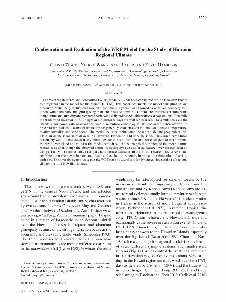
FIG. 1. (a) Model domains and synoptic patterns most relevant to weather and climate in the Hawaiian Islands.

(b) The terrain heights and the locations of the METAR stations and radiosonde stations.


from 1 May 2006 to 31 October 2006. This year included

an exceptional period of heavy rainfall over much of the

main Hawaiian Islands from mid-February to the end

of March (http://www.ncdc.noaa.gov/oa/climate/research/

2006/mar/mar06.html). Two different inner domain runs

were conducted with the original land surface data pro-

vided by the official WRF release (hereafter OLD) and

the new land surface data developed for the Hawaiian

region (hereafter NEW, see section 2b) to demonstrate

the improvements of the simulation with the new land

surface dataset. Note that in both runs, the outer model

domain is identical with the new land surface data (e.g.,

the boundaries for both D2 runs were forced by results

from identical D1 integrations by disabling any feedbacks

from D2 onto D1).

b. Construction of a new land surface dataset

The land surface properties are fundamental input

parameters required for the Noah LSM (Chen and

Dudhia 2001). However, the Hawaiian region is not well

represented in the land surface datasets of the official

WRF model release. These include land cover/use,

surface albedo, vegetation types/fraction, and soil types.

The poor representations of the land surface properties

are mainly caused by the low-resolution datasets (sur-

face albedo, vegetation types/fraction, and soil types) or

poorly retrieved datasets (land cover/use) used in the

official release of the WRF model for the Hawaiian re-

gion. To improve these data, we have implemented the

new land surface properties based on the U.S. Geo-

logical Survey (USGS) data and other sources.

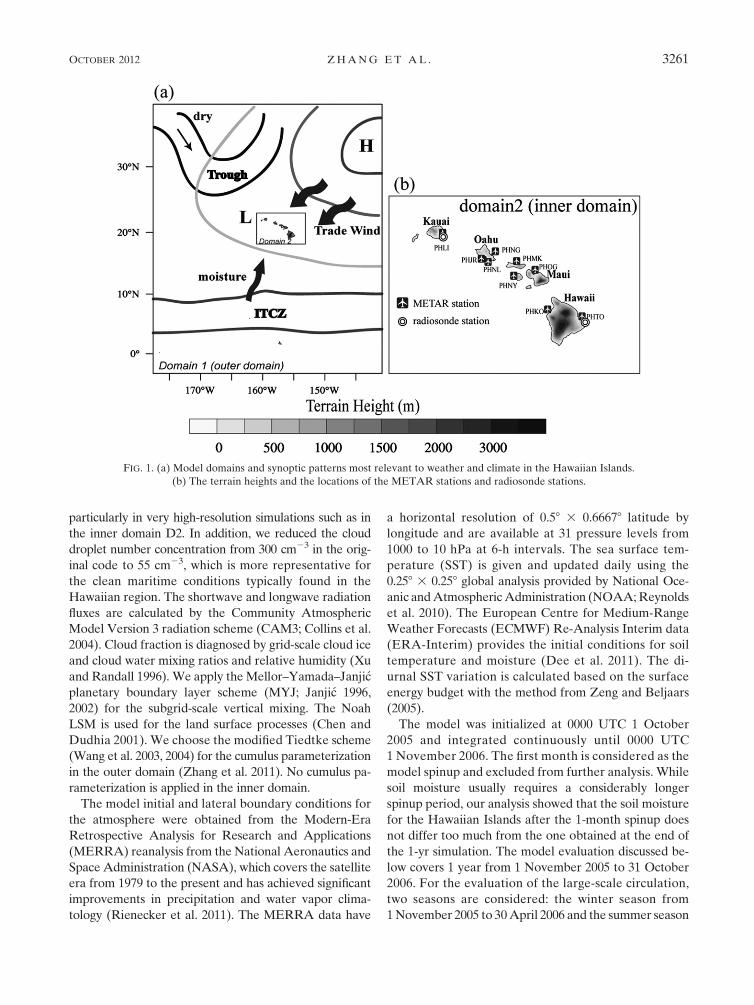
The USGS classifies the land surface at each location

into one of 24 categories. The official WRF release

represents Hawaii by only two of these categories: urban

and mixed forests (Fig. 2a). For our new land surface

dataset we adapted the publicly available 1-s NLCD

(i.e., the 2001 National Land Cover Database; Homer

et al. 2004) to match the USGS 24 categories in the

Hawaiian region (Fig. 2b). Interpolation is necessary

from the 1-s to the HRCM grids. In the NLCD data,

there are four types of urban categories based on the

density of development. Here, we assigned only the

medium and high NLCD urban densities to the urban

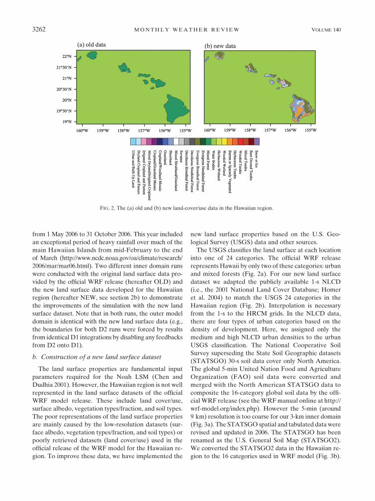
USGS classification. The National Cooperative Soil

Survey superseding the State Soil Geographic datasets

(STATSGO) 30-s soil data cover only North America.

The global 5-min United Nation Food and Agriculture

Organization (FAO) soil data were converted and

merged with the North American STATSGO data to

composite the 16-category global soil data by the offi-

cial WRF release (see the WRF manual online at http://

wrf-model.org/index.php). However the 5-min (around

9 km) resolution is too coarse for our 3-km inner domain

(Fig. 3a). The STATSGO spatial and tabulated data were

revised and updated in 2006. The STATSGO has been

renamed as the U.S. General Soil Map (STATSGO2).

We converted the STATSGO2 data in the Hawaiian re-

gion to the 16 categories used in WRF model (Fig. 3b).

FIG. 2. The (a) old and (b) new land-cover/use data in the Hawaiian region.


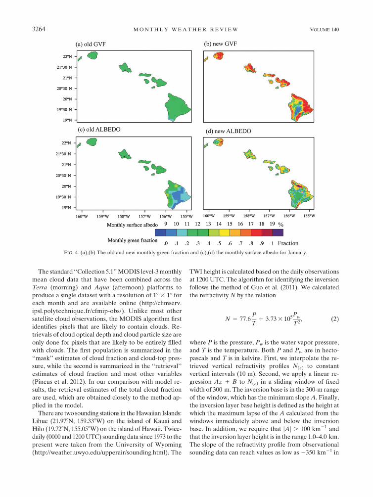
The old green vegetation fraction (GVF) was derived

from the NOAA Advanced Very High Resolution Ra-

diometer (AVHRR) normalized difference vegetation

index (NDVI) data and is given by

GVF 5 (NDVI 2 NDVI0)/(NDVI1 2 NDVI0), (1)

where NDVI0 (bare soil) and NDVI1 (dense vegetation)

are specified as global constants independent of vege-

tation/soil type (Gutman and Ignatov 1998). The GVF

for the Hawaiian Islands is also only crudely represented

in the standard WRF version (Fig. 4a). A 0.058 resolu-

tion 5-yr-averaged (2000–04) Moderate Resolution Im-

aging Spectroradiometer (MODIS) NDVI dataset is

used to derive the GVF for the Hawaiian region based

on Eq. (1). In our method, NDVI0 is 0.04, and NDVI1 is

the maximum NDVI in the whole Hawaiian Islands.

There are 23 observations at 16-day intervals (viz., the

Julian days 001, 017, . . . , 353) for each year for the whole

dataset. In the end, the derived GVF data are interpolated

to monthly data for the WRF (Fig. 4b).

The original surface albedo data in the WRF are

derived from measurements of reflected visible and

near-infrared radiation by AVHRR on board the NOAA

polar-orbiting satellites (Csiszar and Gutman 1999). This

dataset, however, does not represent the Hawaiian region

well as shown in Fig. 4c. We use 5-yr-averaged (2000–04)

MODIS broadband albedo data (collection 4) for visible

(VIS; 0.4–0.7 mm) and near infrared (NIR; 0.7–5.0 mm)

at 0.058 resolution. As for the NDVI dataset, there are

23 total 16-day intervals (001, 017, . . . , 353) for each year

for the whole albedo dataset. The MODIS albedo was

generated by a semi-empirical, kernel-driven linear bi-

directional reflectance distribution function model (Schaaf

et al. 2002). This model relies on the weighted sum of

three parameters retrieved from the multidate multi-

angular cloud-free atmosphere with corrected surface

reflectance at 1-km resolution, acquired by MODIS

during a 16-day period. The MODIS albedo represents

the best quality retrieval possible over each 16-day

period and consists of local noon black-sky (direct)

and white-sky (wholly diffuse) albedo. We evenly av-

eraged both, black-sky and white-sky albedos, as well

as the 16-day period albedo to composite a monthly

albedo dataset for the WRF (Fig. 4d). Note that some

pixels have no data available at all (less than 1%). To

resolve this problem, we assign the value based on land-

use/cover data to those pixels. As a final step, we also

checked the consistency of the albedo with the GVF

data.

c. Data for evaluation and analysis methods

In addition to the MERRA reanalysis data mentioned

above, more data are used for verification of the model

simulations discussed in the following sections. The simu-

lated surface winds are compared with the seasonal surface

winds from the Quick Scatterometer (QuikSCAT) mea-

surements over the ocean. The SeaWinds Scatterometer

on board the QuikSCAT satellite is a microwave radar

launched and operated by the National Aeronautics and

Space Administration (NASA). We use monthly mean

QuikSCAT data at 25-km resolution provided by the

Remote Sensing Systems (http://www.ssmi.com/qscat/

qscat_browse.html).

FIG. 3. The (a) old and (b) new top layer soil types in the Hawaiian region.


The standard ‘‘Collection 5.1’’ MODIS level-3 monthly

mean cloud data that have been combined across the

Terra (morning) and Aqua (afternoon) platforms to

produce a single dataset with a resolution of 18 3 18 for

each month and are available online (http://climserv.

ipsl.polytechnique.fr/cfmip-obs/). Unlike most other

satellite cloud observations, the MODIS algorithm first

identifies pixels that are likely to contain clouds. Re-

trievals of cloud optical depth and cloud particle size are

only done for pixels that are likely to be entirely filled

with clouds. The first population is summarized in the

‘‘mask’’ estimates of cloud fraction and cloud-top pres-

sure, while the second is summarized in the ‘‘retrieval’’

estimates of cloud fraction and most other variables

(Pincus et al. 2012). In our comparison with model re-

sults, the retrieval estimates of the total cloud fraction

are used, which are obtained closely to the method ap-

plied in the model.

There are two sounding stations in the Hawaiian Islands:

Lihue (21.978N, 159.338W) on the island of Kauai and

Hilo (19.728N, 155.058W) on the island of Hawaii. Twice-

daily (0000 and 1200 UTC) sounding data since 1973 to the

present were taken from the University of Wyoming

(http://weather.uwyo.edu/upperair/sounding.html). The

TWI height is calculated based on the daily observations

at 1200 UTC. The algorithm for identifying the inversion

follows the method of Guo et al. (2011). We calculated

the refractivity N by the relation

N 5 77:6P

T1 3:73 3 105Pw

T2, (2)

where P is the pressure, Pw is the water vapor pressure,

and T is the temperature. Both P and Pw are in hecto-

pascals and T is in kelvins. First, we interpolate the re-

trieved vertical refractivity profiles N(z) to constant

vertical intervals (10 m). Second, we apply a linear re-

gression Az 1 B to N(z) in a sliding window of fixed

width of 300 m. The inversion base is in the 300-m range

of the window, which has the minimum slope A. Finally,

the inversion layer base height is defined as the height at

which the maximum lapse of the A calculated from the

windows immediately above and below the inversion

base. In addition, we require that jAj . 100 km21 and

that the inversion layer height is in the range 1.0–4.0 km.

The slope of the refractivity profile from observational

sounding data can reach values as low as 2350 km21 in

FIG. 4. (a),(b) The old and new monthly green fraction and (c),(d) the monthly surface albedo for January.


some cases. Note that because of the fine vertical

pressure intervals in observational soundings (less than

5 hPa around the inversion layer height) and the coarse

vertical pressure intervals in HRCM (25 hPa around

the inversion layer height), we slightly reduced the

slope criterion to jAj. 60 km21, which is very close to

the criterion applied to the Constellation Observing

System for Meteorology Ionosphere and Climate

(COSMIC) data by Guo et al. (2011), who used jAj .50 km21.

Three surface observational accumulated precipitation

datasets for the Hawaiian region are used in our verifi-

cation of the simulated rainfall. The first dataset is the

National Climatic Data Center (NCDC) cooperative

monthly precipitation data (http://www.ncdc.noaa.gov/

oa/ncdc.html), which includes observations from about

190 stations in total. The second dataset is the USGS

daily precipitation data (http://hi.water.usgs.gov/recent/

index.html). The observations at about 30 stations are

averaged to get monthly means. Both the NCDC and

USGS datasets are quality controlled. The third rainfall

dataset is from the Hydronet system, which began col-

lecting 15-min rainfall data in July 1994 (http://www.

prh.noaa.gov/hnl/hydro/hydronet/hydronet-data.php).

Currently the data are collected from 70 rain gauges

located throughout the Hawaiian Islands. After a basic

quality control, we have used data from 65 stations in our

study. We converted the 15-min rainfall data to hourly

and monthly precipitation values.

We selected observations from nine airports [aviation

routine weather report (METAR) Table 1] for verifi-

cation of the simulated daily mean surface variables.

TABLE 1. Names, locations, and elevations of all METAR stations

used for the model verification in this study.

Station ID Station name Lat (N) Lon (W) Elev (m)

PHJR Oahu, Kalaeloa

Airport

21.318 158.078 10.0

PHNG Oahu, Kaneohe

Airport

21.458 157.778 5.0

PHNL Oahu, Honolulu

International

Airport

21.338 157.948 3.0

PHTO Hawaii, Hilo

International

Airport

19.728 155.068 11.0

PHKO Hawaii, Kailua Kona,

Keahole Airport

19.748 156.058 13.0

PHLI Kauai, Lihue Airport 21.988 159.348 45.0

PHNY Lanai, Lanai Airport 20.798 156.958 399.0

PHMK Molokai, Molakai

Airport

21.158 157.108 138.0

PHOG Maui, Kahului Airport 20.898 156.448 16.0

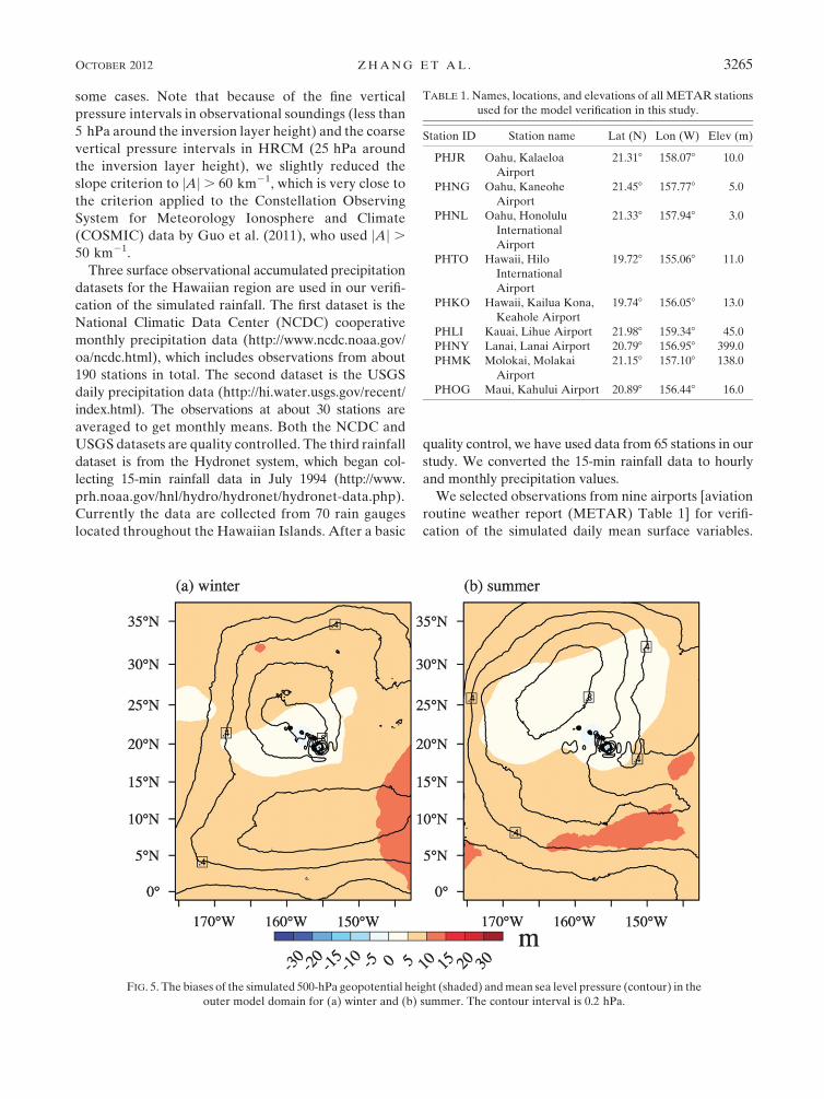
FIG. 5. The biases of the simulated 500-hPa geopotential height (shaded) and mean sea level pressure (contour) in the

outer model domain for (a) winter and (b) summer. The contour interval is 0.2 hPa.


Most observed hourly parameters are available from the

NCDC website. Note that the METAR observations are

taken at around 50th minute of each hour (e.g., 0150,

0250 UTC) but our model output is at 0100, 0200 UTC.

The METAR data are quality controlled and averaged

to get the daily mean data.

The spatial correlation coefficient between a simu-

lated (m) and an observed (o) quantity a is defined as

SC 5

�i

�j

(ami,j 2 am

I,J)(aoi,j 2 ao

I,J)

�i

�j

(ami,j 2 am

I,J)2 �i

�j

(aoi,j 2 ao

I,J)2

" #1/2, (3)

where subscripts i, j are the horizontal gridpoint indices

in the zonal and meridional directions, respectively. The

overbar denotes the spatial average over the WRF grids.

The temporal correlation coefficient between a simu-

lated (m) and an observed (o) quantity a is defined as

R 5�(am

t 2 am)(aot 2 ao)ffiffiffiffiffiffiffiffiffiffiffiffiffiffiffiffiffiffiffiffiffiffiffiffiffiffiffiffiffiffiffiffiffiffiffiffiffiffiffiffiffiffiffiffiffiffiffiffiffiffiffiffiffi

�(amt 2 am)2�(ao

t 2 ao)2q , (4)

where the subscript t is the given time, and the overbar

denotes the time average.

3. Verification of model simulations

The one-way nesting adopted here means that there is

no feedback from the inner high-resolution domain onto

the outer domain. The outer domain (15 km, D1) offers

the inner domain (3 km, D2) lateral boundary condi-

tions at every outer domain time step. As a result, the

coarse ‘‘outer domain (D1)’’ simulation is indeed in-

dependent of a fine-resolution ‘‘inner domain (D2)’’

simulation. We therefore evaluate the simulations from

both domains below.

a. Large-scale circulation

Here we compare the summer- and winter-averaged

large-scale circulations from the HRCM simulation

with available observations. We focus on the evalua-

tion of the D1 simulation in this and next subsections.

The 500-hPa geopotential height (GHT) and mean sea

level pressure (MSLP) biases are shown in Fig. 5, which

are calculated as the difference between the HRCM

simulation and MERRA reanalysis. In both winter and

summer, the GHT bias in most of the domain is less than

10 m and even less than 5 m around the Hawaiian Islands.

The bias pattern is similar in summer and winter. The

positive bias in MSLP is centered around the Hawaiian

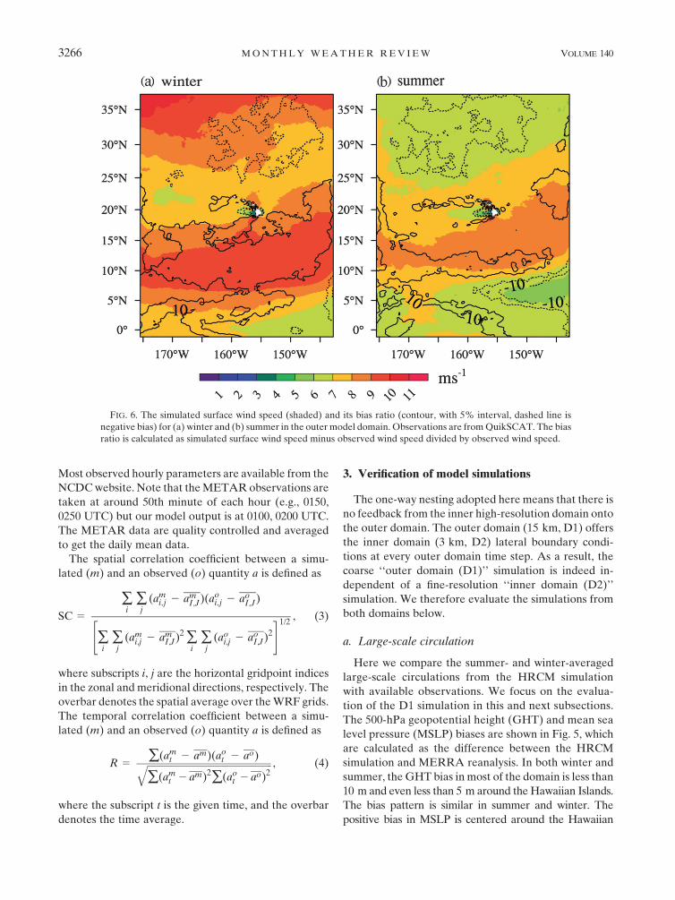
FIG. 6. The simulated surface wind speed (shaded) and its bias ratio (contour, with 5% interval, dashed line is

negative bias) for (a) winter and (b) summer in the outer model domain. Observations are from QuikSCAT. The bias

ratio is calculated as simulated surface wind speed minus observed wind speed divided by observed wind speed.


Islands in winter, while the positive MSLP bias is centered

northwest of the Hawaiian Islands in summer. In both

seasons, the maximum MSLP biases are less than 1 hPa.

Figure 6 shows the HRCM simulated 10-m height

wind speed, which is seasonally averaged. We define the

bias in the seasonal mean 10-m height wind speed as the

difference between the simulated and the observed

seasonal mean surface wind speed from QuikSCAT.

The bias ratio is defined as the bias divided by the

QuikSCAT surface wind speed. The observed surface

wind speed around the Hawaiian Islands is between 6

and 10 m s21 in winter and about 1 m s21 weaker be-

tween 58 and 258N in summer. The wind speed bias ratio

around the Hawaiian Islands in both winter and summer

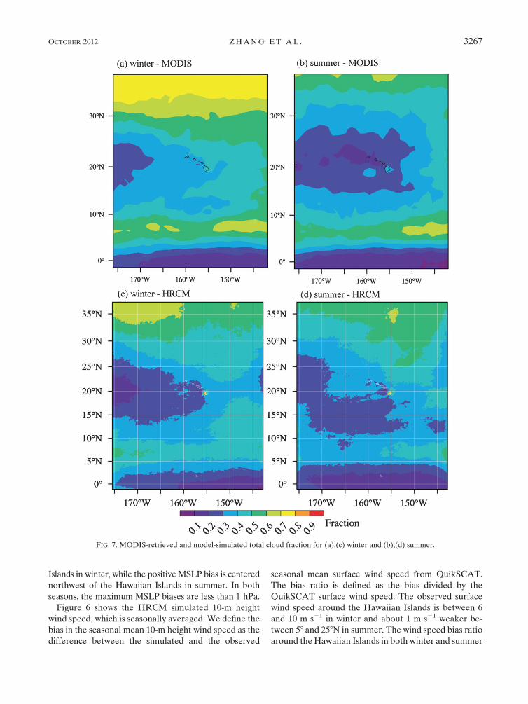
FIG. 7. MODIS-retrieved and model-simulated total cloud fraction for (a),(c) winter and (b),(d) summer.


are generally less than 5% with the actual bias less than

about 0.5 m s21. The negative bias north of the Hawaiian

Islands and the positive bias south of the Hawaiian Islands

are generally larger, but less than 15%.

Both the simulated and the MODIS-retrieved total

cloud fractions for both summer and winter are shown in

Fig. 7. The spatial correlation (SC) between the simu-

lated and the MODIS cloud fractions is 0.74 in winter

and 0.75 in summer. In winter, the simulated total cloud

fraction is about 10%–20% less than that observed in

most of domain D1. In summer, the simulated total

cloud fraction north of 158N is close or about 10% higher

than that observed. As in winter, the model also un-

derestimates the total cloud fraction in the ITCZ in

summer. The MODIS-retrieved total cloud fraction

around the Hawaiian Islands in summer (except for the

island of Hawaii) is generally less than 10%, but the

HRCM-simulated total cloud fraction is between 0.2

and 0.4. Note that MODIS cannot resolve the trade

cumuli well commonly found in the Hawaiian region due

to its coarse spatial resolution and the thresholds used in

the retrieval algorithm (Pincus et al. 2012). Neverthe-

less, the above comparison still gives some confidence

that the HRCM has promising skills in reproducing the

cloud distribution at the large scale around the Hawaiian

Islands.

b. Vertical structure

One of the main features of the trade wind region is

the TWI, which is highly correlated with precipitation at

Hilo with a correlation coefficient of greater than 0.7

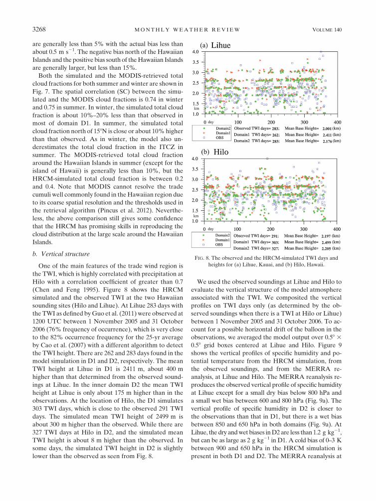
(Chen and Feng 1995). Figure 8 shows the HRCM

simulated and the observed TWI at the two Hawaiian

sounding sites (Hilo and Lihue). At Lihue 283 days with

the TWI as defined by Guo et al. (2011) were observed at

1200 UTC between 1 November 2005 and 31 October

2006 (76% frequency of occurrence), which is very close

to the 82% occurrence frequency for the 25-yr average

by Cao et al. (2007) with a different algorithm to detect

the TWI height. There are 262 and 283 days found in the

model simulation in D1 and D2, respectively. The mean

TWI height at Lihue in D1 is 2411 m, about 400 m

higher than that determined from the observed sound-

ings at Lihue. In the inner domain D2 the mean TWI

height at Lihue is only about 175 m higher than in the

observations. At the location of Hilo, the D1 simulates

303 TWI days, which is close to the observed 291 TWI

days. The simulated mean TWI height of 2499 m is

about 300 m higher than the observed. While there are

327 TWI days at Hilo in D2, and the simulated mean

TWI height is about 8 m higher than the observed. In

some days, the simulated TWI height in D2 is slightly

lower than the observed as seen from Fig. 8.

We used the observed soundings at Lihue and Hilo to

evaluate the vertical structure of the model atmosphere

associated with the TWI. We composited the vertical

profiles on TWI days only (as determined by the ob-

served soundings when there is a TWI at Hilo or Lihue)

between 1 November 2005 and 31 October 2006. To ac-

count for a possible horizontal drift of the balloon in the

observations, we averaged the model output over 0.58 3

0.58 grid boxes centered at Lihue and Hilo. Figure 9

shows the vertical profiles of specific humidity and po-

tential temperature from the HRCM simulation, from

the observed soundings, and from the MERRA re-

analysis, at Lihue and Hilo. The MERRA reanalysis re-

produces the observed vertical profile of specific humidity

at Lihue except for a small dry bias below 800 hPa and

a small wet bias between 600 and 800 hPa (Fig. 9a). The

vertical profile of specific humidity in D2 is closer to

the observations than that in D1, but there is a wet bias

between 850 and 650 hPa in both domains (Fig. 9a). At

Lihue, the dry and wet biases in D2 are less than 1.2 g kg21,

but can be as large as 2 g kg21 in D1. A cold bias of 0–3 K

between 900 and 650 hPa in the HRCM simulation is

present in both D1 and D2. The MERRA reanalysis at

FIG. 8. The observed and the HRCM-simulated TWI days and

heights for (a) Lihue, Kauai, and (b) Hilo, Hawaii.


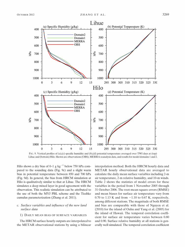
Hilo shows a dry bias of 0–1 g kg21 below 750 hPa com-

pared to the sounding data (Fig. 9c) and a slight warm

bias in potential temperature between 850 and 700 hPa

(Fig. 9d). In general, the bias from HRCM simulation at

Hilo is qualitatively similar to that at Lihue. The HRCM

simulates a deep mixed layer in good agreement with the

observation. This realistic simulation can be attributed to

the use of both the MYJ PBL scheme and the Tiedtke

cumulus parameterization (Zhang et al. 2011).

c. Surface variables and influence of the new landsurface data

1) DAILY MEAN BIAS OF SURFACE VARIABLES

The HRCM surface hourly outputs are interpolated to

the METAR observational stations by using a bilinear

interpolation method. Both the HRCM hourly data and

METAR hourly observational data are averaged to

calculate the daily mean surface variables including 2-m

air temperature, 2-m relative humidity, and 10-m winds.

Table 2 shows the statistics of model errors for these

variables in the period from 1 November 2005 through

31 October 2006. The root-mean-square errors (RMSE)

and mean biases for surface air temperature vary from

0.70 to 1.13 K and from 21.10 to 0.67 K, respectively,

among different stations. The magnitude of both RMSE

and bias are comparable with those of Nguyen et al.

(2010) for the island of Oahu and Yang et al. (2005) for

the island of Hawaii. The temporal correlation coeffi-

cient for surface air temperature varies between 0.80

and 0.90. Surface relative humidity at all stations is gen-

erally well simulated. The temporal correlation coefficient

FIG. 9. Vertical profiles of (a),(c) specific humidity and (b),(d) potential temperature averaged over TWI days at (top)

Lihue and (bottom) Hilo. Shown are observations (OBS), MERRA reanalysis data, and results for model domains 1 and 2.


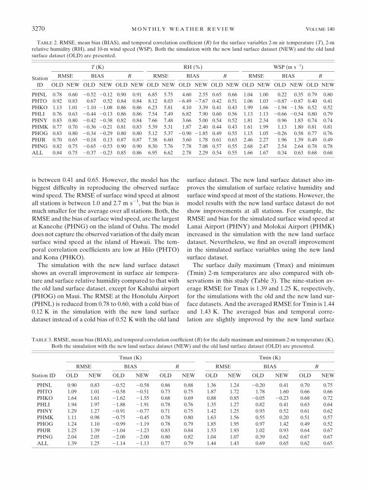
is between 0.41 and 0.65. However, the model has the

biggest difficulty in reproducing the observed surface

wind speed. The RMSE of surface wind speed at almost

all stations is between 1.0 and 2.7 m s21, but the bias is

much smaller for the average over all stations. Both, the

RMSE and the bias of surface wind speed, are the largest

at Kaneohe (PHNG) on the island of Oahu. The model

does not capture the observed variation of the daily mean

surface wind speed at the island of Hawaii. The tem-

poral correlation coefficients are low at Hilo (PHTO)

and Kona (PHKO).

The simulation with the new land surface dataset

shows an overall improvement in surface air tempera-

ture and surface relative humidity compared to that with

the old land surface dataset, except for Kahului airport

(PHOG) on Maui. The RMSE at the Honolulu Airport

(PHNL) is reduced from 0.78 to 0.60, with a cold bias of

0.12 K in the simulation with the new land surface

dataset instead of a cold bias of 0.52 K with the old land

surface dataset. The new land surface dataset also im-

proves the simulation of surface relative humidity and

surface wind speed at most of the stations. However, the

model results with the new land surface dataset do not

show improvements at all stations. For example, the

RMSE and bias for the simulated surface wind speed at

Lanai Airport (PHNY) and Molokai Airport (PHMK)

increased in the simulation with the new land surface

dataset. Nevertheless, we find an overall improvement

in the simulated surface variables using the new land

surface dataset.

The surface daily maximum (Tmax) and minimum

(Tmin) 2-m temperatures are also compared with ob-

servations in this study (Table 3). The nine-station av-

erage RMSE for Tmax is 1.39 and 1.25 K, respectively,

for the simulations with the old and the new land sur-

face datasets. And the averaged RMSE for Tmin is 1.44

and 1.43 K. The averaged bias and temporal corre-

lation are slightly improved by the new land surface

TABLE 2. RMSE, mean bias (BIAS), and temporal correlation coefficient (R) for the surface variables 2-m air temperature (T), 2-m

relative humidity (RH), and 10-m wind speed (WSP). Both the simulation with the new land surface dataset (NEW) and the old land

surface dataset (OLD) are presented.

Station

ID

T (K) RH (%) WSP (m s21)

RMSE BIAS R RMSE BIAS R RMSE BIAS R

OLD NEW OLD NEW OLD NEW OLD NEW OLD NEW OLD NEW OLD NEW OLD NEW OLD NEW

PHNL 0.78 0.60 20.52 20.12 0.90 0.91 6.85 5.75 4.60 2.55 0.65 0.66 1.04 1.00 0.22 0.35 0.79 0.80

PHTO 0.92 0.83 0.67 0.52 0.84 0.84 8.12 8.03 26.49 27.67 0.42 0.51 1.06 1.03 20.87 20.87 0.40 0.41

PHKO 1.13 1.01 21.10 21.08 0.86 0.86 6.23 5.81 4.10 3.39 0.41 0.43 1.99 1.66 21.94 21.56 0.52 0.52

PHLI 0.76 0.63 20.44 20.13 0.86 0.86 7.54 7.49 6.82 7.90 0.60 0.56 1.13 1.13 20.66 20.54 0.80 0.79

PHNY 0.83 0.80 20.42 20.38 0.82 0.84 7.66 7.48 3.66 5.00 0.54 0.52 1.81 2.34 0.96 1.83 0.74 0.74

PHMK 0.77 0.70 20.36 20.21 0.81 0.83 5.39 5.31 1.87 2.40 0.44 0.43 1.61 1.99 1.13 1.80 0.81 0.81

PHOG 0.83 0.80 20.34 20.29 0.80 0.80 5.12 5.37 20.90 21.85 0.49 0.55 1.15 1.05 20.26 0.58 0.77 0.76

PHJR 0.70 0.65 20.18 0.13 0.87 0.87 7.38 6.60 3.60 1.78 0.61 0.63 2.46 2.27 1.96 1.39 0.49 0.49

PHNG 0.82 0.75 20.65 20.53 0.90 0.90 8.30 7.76 7.78 7.08 0.57 0.55 2.68 2.47 2.54 2.64 0.78 0.78

ALL 0.84 0.75 20.37 20.23 0.85 0.86 6.95 6.62 2.78 2.29 0.54 0.55 1.66 1.67 0.34 0.63 0.68 0.68

TABLE 3. RMSE, mean bias (BIAS), and temporal correlation coefficient (R) for the daily maximum and minimum 2-m temperature (K).

Both the simulation with the new land surface dataset (NEW) and the old land surface dataset (OLD) are presented.

Station ID

Tmax (K) Tmin (K)

RMSE BIAS R RMSE BIAS R

OLD NEW OLD NEW OLD NEW OLD NEW OLD NEW OLD NEW

PHNL 0.90 0.83 20.52 20.58 0.86 0.88 1.36 1.24 20.20 0.41 0.70 0.75

PHTO 1.09 1.01 20.58 20.51 0.73 0.75 1.87 1.72 1.78 1.60 0.66 0.66

PHKO 1.64 1.61 21.62 21.55 0.68 0.69 0.88 0.85 20.05 20.23 0.68 0.72

PHLI 1.94 1.97 21.88 21.91 0.78 0.76 1.35 1.27 0.82 0.41 0.63 0.64

PHNY 1.29 1.27 20.91 20.77 0.71 0.75 1.42 1.25 0.93 0.52 0.61 0.62

PHMK 1.11 0.98 20.75 20.45 0.78 0.80 1.63 1.56 0.55 0.20 0.51 0.57

PHOG 1.24 1.10 20.99 21.19 0.78 0.79 1.85 1.95 0.97 1.42 0.49 0.52

PHJR 1.25 1.39 21.04 21.23 0.83 0.84 1.53 1.93 1.02 0.93 0.64 0.67

PHNG 2.04 2.05 22.00 22.00 0.80 0.82 1.04 1.07 0.39 0.62 0.67 0.67

ALL 1.39 1.25 21.14 21.13 0.77 0.79 1.44 1.43 0.69 0.65 0.62 0.65


dataset. Similarly to the daily mean values, the model

results are not improved at all stations by the new land

surface dataset. For instance, the RMSE for Tmax at

the Kalaeloa airport (PHJR) on Oahu increased from

1.25 to 1.39 K, and Tmin increased from 1.53 to 1.93 K.

All stations have a cold Tmax bias between 0.52 and

2.0 K. Most stations have a warm Tmin bias between

0.55 and 1.78 K. Both HRCM simulations have

smaller diurnal surface temperature amplitudes than

the observations. This is because the simulated Tmax

is about 1 K lower and the simulated Tmin is around

0.7 K higher. The new land surface data do not re-

duce the bias of the diurnal amplitude of the surface

temperature.

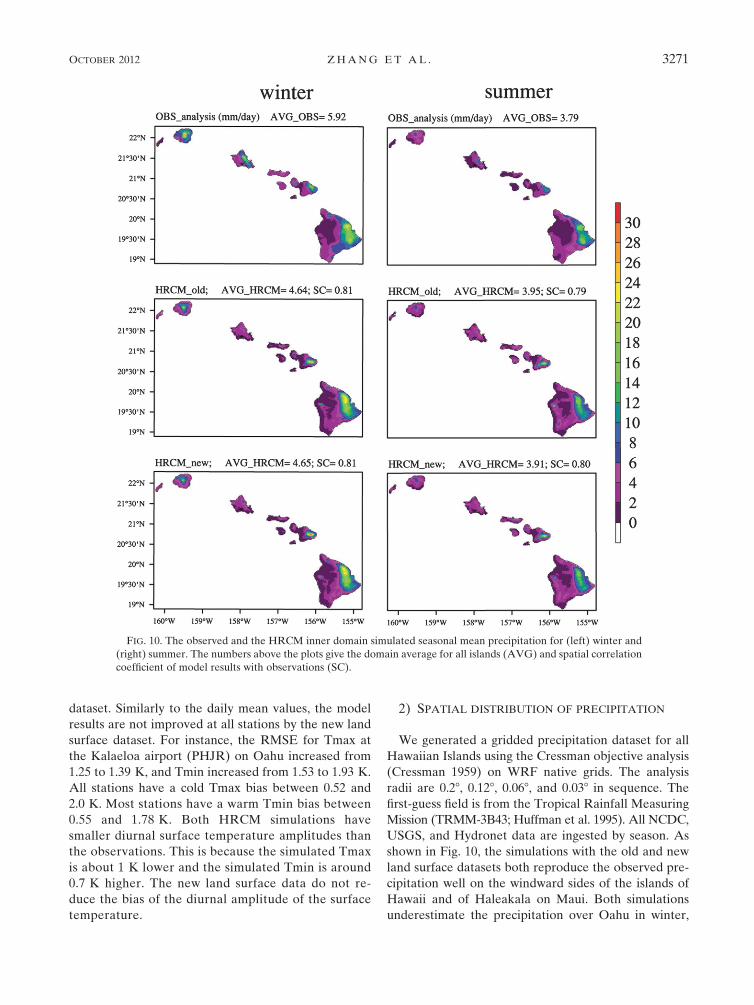
2) SPATIAL DISTRIBUTION OF PRECIPITATION

We generated a gridded precipitation dataset for all

Hawaiian Islands using the Cressman objective analysis

(Cressman 1959) on WRF native grids. The analysis

radii are 0.28, 0.128, 0.068, and 0.038 in sequence. The

first-guess field is from the Tropical Rainfall Measuring

Mission (TRMM-3B43; Huffman et al. 1995). All NCDC,

USGS, and Hydronet data are ingested by season. As

shown in Fig. 10, the simulations with the old and new

land surface datasets both reproduce the observed pre-

cipitation well on the windward sides of the islands of

Hawaii and of Haleakala on Maui. Both simulations

underestimate the precipitation over Oahu in winter,

FIG. 10. The observed and the HRCM inner domain simulated seasonal mean precipitation for (left) winter and

(right) summer. The numbers above the plots give the domain average for all islands (AVG) and spatial correlation

coefficient of model results with observations (SC).


which is mainly a result of the underestimation of the

mean precipitation for all the islands in winter (4.64 and

4.65 mm day21 in the model simulations vs 5.92 mm

day21 in the observations). This is because the HRCM

simulation does not reproduce the heavy rain events in

March 2006 well when a large low pressure system lin-

gered west of the Hawaiian Islands (not shown). Even

though this storm is captured by the model, its exact lo-

cation is not. This clearly shows the challenges of simu-

lating heavy precipitation events by individual storms

with a climate model despite the model being forced by

observed boundary conditions. The SC of the seasonal

mean precipitation is around 0.80. The simulation with

the new land surface dataset does not show a higher SC

than that with the old land surface dataset.

3) DIURNAL RAINFALL VARIATIONS

The Hydronet rainfall data at 65 observational stations

are used to study the diurnal rainfall variations over the

Hawaiian Islands for TWI days from 1 November 2005 to

31 October 2006. Here, we use TWI days observed at

Lihue, Kauai (PHLI), and Hilo, Hawaii (PHTO). If both

stations have a TWI at the same time, we consider it

a TWI day, which gives 251 TWI days in the studied pe-

riod. Note that, the simulated TWI days can differ from

the observed ones. We choose TWI days to exclude pe-

riods with midlatitude or tropical disturbances (they are

discussed separately below) and focus on trade wind re-

gime in the Hawaiian region. The rainfall intensity peak is

defined as the hour with the maximum observed hourly

rainfall averaged over all TWI days. The rainfall fre-

quency peak is defined as the hour when rainfall occurs

most frequently. Because the observational precision is

0.01 in. (0.254 mm), the threshold for recorded rainfall is

also 0.254 mm. We normalized the rainfall intensity at

each station (the averaged hourly rainfall on all TWI days

divided by the daily rainfall amount) before the averaged

rainfall intensity was calculated island by island.

Each island has a unique rainfall diurnal cycle

(Figs. 11 and 12 ) and the rainfall intensity peak from the

observations shows a large diversity among different

islands (Fig. 11a). The island of Kauai has an intensity

peak at late night to early morning, while the island of

Oahu reaches its intensity peak in the afternoon at most

of the observational stations, although the two islands are

in close distance and have a similar size. In the northern

part of the island of Maui the rainfall intensity peak oc-

curs between midnight and the early morning and in the

early afternoon in other parts of Maui. Over the island of

Hawaii the rainfall intensity peak occurs in the late af-

ternoon to early night. Over most of the islands the

rainfall intensity peak is consistent with the frequency

peak or within a few hours at the most except for the

island of Oahu where the intensity peak occurs in the

afternoon, while the frequency peak occurs in the early

morning (Fig. 11). As can be seen from Fig. 12c, the island

of Oahu has two intensity peaks: one is in the early

morning and the other is in the early afternoon. The af-

ternoon intensity peak is stronger than the early morning

peak, indicating the effects of land heating and terrain on

the diurnal precipitation cycle.

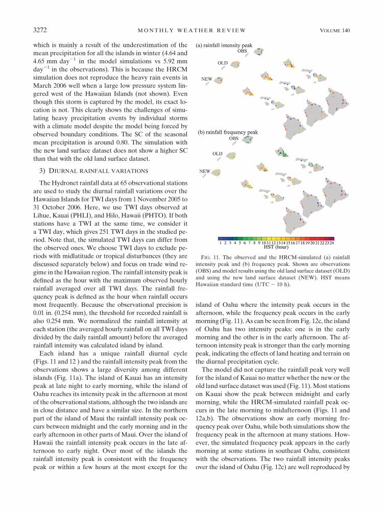
The model did not capture the rainfall peak very well

for the island of Kauai no matter whether the new or the

old land surface dataset was used (Fig. 11). Most stations

on Kauai show the peak between midnight and early

morning, while the HRCM-simulated rainfall peak oc-

curs in the late morning to midafternoon (Figs. 11 and

12a,b). The observations show an early morning fre-

quency peak over Oahu, while both simulations show the

frequency peak in the afternoon at many stations. How-

ever, the simulated frequency peak appears in the early

morning at some stations in southeast Oahu, consistent

with the observations. The two rainfall intensity peaks

over the island of Oahu (Fig. 12c) are well reproduced by

FIG. 11. The observed and the HRCM-simulated (a) rainfall

intensity peak and (b) frequency peak. Shown are observations

(OBS) and model results using the old land surface dataset (OLD)

and using the new land surface dataset (NEW). HST means

Hawaiian standard time (UTC 2 10 h).


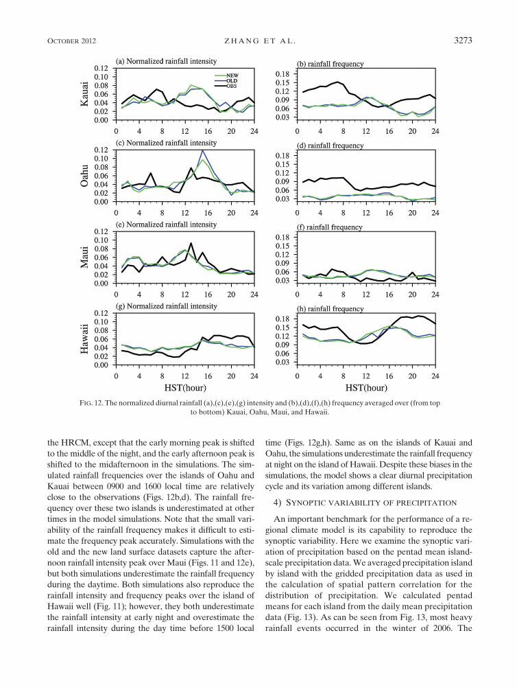
the HRCM, except that the early morning peak is shifted

to the middle of the night, and the early afternoon peak is

shifted to the midafternoon in the simulations. The sim-

ulated rainfall frequencies over the islands of Oahu and

Kauai between 0900 and 1600 local time are relatively

close to the observations (Figs. 12b,d). The rainfall fre-

quency over these two islands is underestimated at other

times in the model simulations. Note that the small vari-

ability of the rainfall frequency makes it difficult to esti-

mate the frequency peak accurately. Simulations with the

old and the new land surface datasets capture the after-

noon rainfall intensity peak over Maui (Figs. 11 and 12e),

but both simulations underestimate the rainfall frequency

during the daytime. Both simulations also reproduce the

rainfall intensity and frequency peaks over the island of

Hawaii well (Fig. 11); however, they both underestimate

the rainfall intensity at early night and overestimate the

rainfall intensity during the day time before 1500 local

time (Figs. 12g,h). Same as on the islands of Kauai and

Oahu, the simulations underestimate the rainfall frequency

at night on the island of Hawaii. Despite these biases in the

simulations, the model shows a clear diurnal precipitation

cycle and its variation among different islands.

4) SYNOPTIC VARIABILITY OF PRECIPITATION

An important benchmark for the performance of a re-

gional climate model is its capability to reproduce the

synoptic variability. Here we examine the synoptic vari-

ation of precipitation based on the pentad mean island-

scale precipitation data. We averaged precipitation island

by island with the gridded precipitation data as used in

the calculation of spatial pattern correlation for the

distribution of precipitation. We calculated pentad

means for each island from the daily mean precipitation

data (Fig. 13). As can be seen from Fig. 13, most heavy

rainfall events occurred in the winter of 2006. The

FIG. 12. The normalized diurnal rainfall (a),(c),(e),(g) intensity and (b),(d),(f),(h) frequency averaged over (from top

to bottom) Kauai, Oahu, Maui, and Hawaii.


HRCM captures most of the precipitation events rea-

sonably well except for some events in March on the

islands of Oahu and Maui. As already discussed above,

this is caused mainly by a bias in the location of the

simulated storm that was responsible for the heavy pre-

cipitation events in March 2006. The storm and the as-

sociated frontal systems in the model stayed too far west

of Oahu and Maui instead of moving toward the islands

as observed. The temporal correlation coefficients reach

0.65, 0.50, 0.53, and 0.58 for Kauai, Oahu, Maui, and

Hawaii, respectively, using the new land surface datasets,

which slightly improves the simulation of synoptic vari-

ability of precipitation compared to the old land surface

dataset. Nevertheless, the relatively high temporal cor-

relation coefficients for the island averages suggest that

the model has skills in reproducing the synoptic vari-

ability of precipitation in the Hawaiian region.

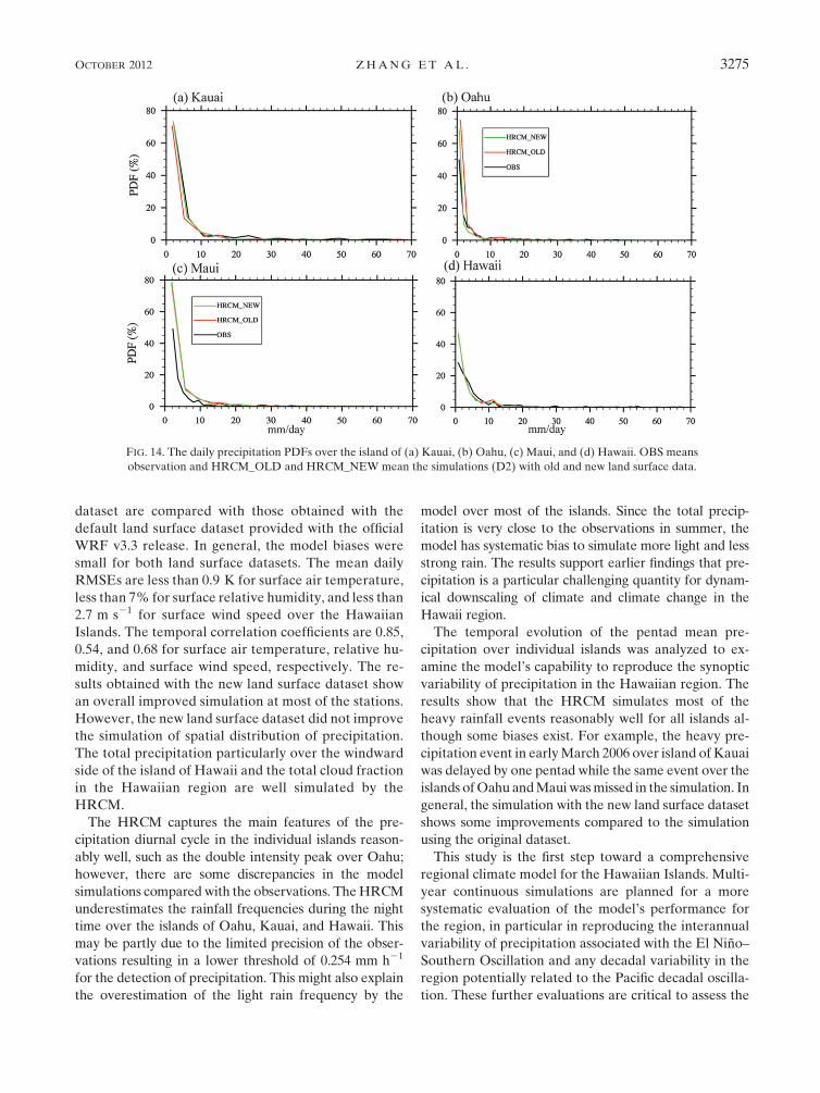
Figure 14 shows the probability density functions

(PDFs) for daily precipitation intensity averaged over

the four main Hawaiian Islands from observations and

the model simulations with both the new and the old

land surface datasets. The simulated rainfall intensity

PDFs over the islands of Kauai and Oahu are similar

to the observed ones except that the model slightly

underestimates light rain over Kauai (Fig. 14a) and

overestimates light rain over Oahu (Fig. 14b) and Maui

(Fig. 14c). The model slightly underestimates precip-

itation below 3 mm day21 and slightly overestimates

precipitation between 3–9 mm day21 for the island of

Hawaii. In general, the HRCM tends to simulate slightly

more light rain (less than 3 mm day21) except for the

island of Kauai.

4. Summary and conclusions

We have documented the HRCM, which was adapted

from the ARW-WRF version 3.3 for climate simulations

in the Hawaii region and we evaluated a 1-yr continuous

simulation forced by observed lateral boundary condi-

tions. A new land surface dataset based on various data

sources was constructed and implemented into the

model. This new dataset led to overall improved simu-

lations of surface variables in most of the Hawaiian re-

gion compared with the original dataset available with

the official release of WRF V3.3. In addition to the new

land surface data, we used the Tiedtke convective pa-

rameterization scheme in our simulations. The Tiedtke

scheme newly implemented into WRF by Zhang et al.

(2011) shows superior performance in the Hawaii re-

gion with an improved simulation of low-level clouds in

the trade wind regime as already shown in Zhang et al.

(2011). The parameterizations of the warm rain pro-

cesses autoconversion and accretion from Khairoutdinov

and Kogan (2000) as well as an adjustment of the av-

erage cloud droplet number concentration are used to

improve the simulations of trade wind cumuli in the

Hawaii region.

The results show that the HRCM captured the basic

features of the seasonal mean large-scale circulation

reasonably well. The seasonal mean MSLP and 500-hPa

geopotential height biases are very small, although

there are cold and wet biases in the simulated lower

troposphere compared to the MERRA reanalysis data.

Model results obtained with the new land surface

FIG. 13. The time series of the 5-day mean precipitation over the

island of (a) Kauai, (b) Oahu, (c) Maui, and (d) Hawaii. OBS

means observation, and HRCM_OLD and HRCM_NEW mean

the simulations (D2) with old and new land surface data. R1 and R2

mean the correlation coefficients between OBS and HRCM_OLD,

OBS and HRCM_NEW, respectively. R3 means the correlation

coefficient between HRCM_OLD and HRCM_NEW.


dataset are compared with those obtained with the

default land surface dataset provided with the official

WRF v3.3 release. In general, the model biases were

small for both land surface datasets. The mean daily

RMSEs are less than 0.9 K for surface air temperature,

less than 7% for surface relative humidity, and less than

2.7 m s21 for surface wind speed over the Hawaiian

Islands. The temporal correlation coefficients are 0.85,

0.54, and 0.68 for surface air temperature, relative hu-

midity, and surface wind speed, respectively. The re-

sults obtained with the new land surface dataset show

an overall improved simulation at most of the stations.

However, the new land surface dataset did not improve

the simulation of spatial distribution of precipitation.

The total precipitation particularly over the windward

side of the island of Hawaii and the total cloud fraction

in the Hawaiian region are well simulated by the

HRCM.

The HRCM captures the main features of the pre-

cipitation diurnal cycle in the individual islands reason-

ably well, such as the double intensity peak over Oahu;

however, there are some discrepancies in the model

simulations compared with the observations. The HRCM

underestimates the rainfall frequencies during the night

time over the islands of Oahu, Kauai, and Hawaii. This

may be partly due to the limited precision of the obser-

vations resulting in a lower threshold of 0.254 mm h21

for the detection of precipitation. This might also explain

the overestimation of the light rain frequency by the

model over most of the islands. Since the total precip-

itation is very close to the observations in summer, the

model has systematic bias to simulate more light and less

strong rain. The results support earlier findings that pre-

cipitation is a particular challenging quantity for dynam-

ical downscaling of climate and climate change in the

Hawaii region.

The temporal evolution of the pentad mean pre-

cipitation over individual islands was analyzed to ex-

amine the model’s capability to reproduce the synoptic

variability of precipitation in the Hawaiian region. The

results show that the HRCM simulates most of the

heavy rainfall events reasonably well for all islands al-

though some biases exist. For example, the heavy pre-

cipitation event in early March 2006 over island of Kauai

was delayed by one pentad while the same event over the

islands of Oahu and Maui was missed in the simulation. In

general, the simulation with the new land surface dataset

shows some improvements compared to the simulation

using the original dataset.

This study is the first step toward a comprehensive

regional climate model for the Hawaiian Islands. Multi-

year continuous simulations are planned for a more

systematic evaluation of the model’s performance for

the region, in particular in reproducing the interannual

variability of precipitation associated with the El Nino–

Southern Oscillation and any decadal variability in the

region potentially related to the Pacific decadal oscilla-

tion. These further evaluations are critical to assess the

FIG. 14. The daily precipitation PDFs over the island of (a) Kauai, (b) Oahu, (c) Maui, and (d) Hawaii. OBS means

observation and HRCM_OLD and HRCM_NEW mean the simulations (D2) with old and new land surface data.


confidence in dynamical downscaling results with the

HRCM of the future climate projections for the Hawaiian

Islands.

Acknowledgments. This study was supported by

NOAA Grant NA07OAR4310257 and DOE Regional

and Global Climate Modeling (RCGM) Program Grant

ER64840. Additional support was provided by the Japan

Agency for Marine-Earth Science and Technology

(JAMSTEC), by NASA through Grant NNX07AG53G,

and by NOAA through Grant NA09OAR4320075, which

sponsor research at the International Pacific Research

Center. We would to acknowledge the Hawaii Open Su-

percomputer Center for providing access to their facilities.

REFERENCES

Bukovsky, M. S., and D. J. Karoly, 2009: Precipitation simulations

using WRF as a nested regional climate model. J. Appl.

Meteor. Climatol., 48, 2152–2159.

Cao, G., T. W. Giambelluca, D. E. Stevens, and T. A. Schroeder,

2007: Inversion variability in the Hawaiian trade wind regime.

J. Climate, 20, 1145–1160.

Carlis, D. L., Y.-L. Chen, and V. Morris, 2010: Numerical simula-

tions of island-scale airflow and the Maui vortex during sum-

mer trade wind conditions. Mon. Wea. Rev., 138, 2706–2736.

Chen, F., and J. Dudhia, 2001: Coupling an advanced land-surface/

hydrology model with the Penn State/NCAR MM5 modeling

system. Part I: Model description and implementation. Mon.

Wea. Rev., 129, 569–585.

Chen, Y.-L., and A. J. Nash, 1994: Diurnal variation of surface

airflow and rainfall frequencies on the island of Hawaii. Mon.

Wea. Rev., 122, 34–56.

——, and J. Feng, 1995: The influences of inversion height on the

precipitation and airflow over the island of Hawaii. Mon. Wea.

Rev., 123, 1660–1676.

——, and ——, 2001: Numerical simulations of airflow and cloud

distributions over the windward side of the island of Hawaii.

Part I: The effects of trade wind inversion. Mon. Wea. Rev.,

129, 1117–1134.

Chu, P.-S., and J. D. Clark, 1999: Decadal variations of tropical

cyclone activity over the central North Pacific. Bull. Amer.

Meteor. Soc., 80, 1875–1881.

——, A. J. Nash, and F. Porter, 1993: Diagnostic studies of two

contrasting rainfall episodes in Hawaii: Dry 1981 and wet

1982. J. Climate, 6, 1457–1462.

Collins, W. D., and Coauthors, 2004: Description of the NCAR

Community Atmosphere Model (CAM3.0). NCAR Tech.

Note NCAR/TN-4641STR, 226 pp.

Cressman, G. P., 1959: An operational objective analysis system.

Mon. Wea. Rev., 87, 367–374.

Csiszar, I., and G. Gutman, 1999: Mapping global land surface al-

bedo from NOAA AVHRR. J. Geophys. Res., 104 (D6),

6215–6228.

Dee, D. P., and Coauthors, 2011: The ERA-Interim reanalysis:

Configuration and performance of the data assimilation sys-

tem. Quart. J. Roy. Meteor. Soc., 137, 553–597.

Esteban, M. A., and Y. L. Chen, 2008: The impact of trade wind

strength on precipitation over the windward side of the island

of Hawaii. Mon. Wea. Rev., 136, 913–928.

Feng, J., and Y. L. Chen, 2001: Numerical simulations of airflow

and cloud distributions over the windward side of the island of

Hawaii. Part II: Nocturnal flow regime. Mon. Wea. Rev., 129,

1135–1147.

Giambelluca, T. W., and M. A. Schroeder, 1986: Rainfall Atlas of

Hawaii. Rep. R76, Department of Land and Natural Re-

sources Hawaii, 267 pp.

Guo, P., Y.-H. Kuo, S. V. Sokolovskiy, and D. H. Lenschow, 2011:

Estimating atmospheric boundary layer depth using COSMIC

radio occultation data. J. Atmos. Sci., 68, 1703–1713.

Gutman, G., and A. Ignatov, 1998: The derivation of green veg-

etation fraction from NOAA/AVHRR data for use in nu-

merical weather prediction models. Int. J. Remote Sens., 19,

1533–1543.

Homer, C., C. Huang, L. Yang, B. Wylie, and M. Coan, 2004:

Development of a 2001 National Land-Cover Database

for the United States. Photogramm. Eng. Remote Sens., 70,

829–840.

Hong, S.-Y., and J. Lim, 2006: The WRF single-moment 6-class

microphysics scheme (WSM6). J. Korean Meteor. Soc., 42,

129–151.

Huffman, G. J., R. F. Adler, B. Rudolf, U. Schneider, and P. R.

Keehn, 1995: Global precipitation estimates based on a tech-

nique for combining satellite-based estimates, rain gauge

analysis, and NWP model precipitation information. J. Climate,

8, 1284–1295.

Janjic, Z. I., 1996: The surface layer in the NCEP Eta Model.

Preprints, 11th Conf. on Numerical Weather Prediction, Norfolk,

VA, Amer. Meteor. Soc., 354–355.

——, 2002: Nonsingular implementation of the Mellor–Yamada

level 2.5 scheme in the NCEP Meso model. NCEP Office Note

437, 61 pp.

Jimenez, P. A., J. Fidel Gonzalez-Rouco, E. Garcıa-Bustamante,

J. Navarro, J. P. Montavez, J. Vila-Guerau de Arellano,

J. Dudhia, and A. Munoz-Roldan, 2010: Surface wind re-

gionalization over complex terrain: Evaluation and analysis of

a high-resolution WRF simulation. J. Appl. Meteor. Climatol.,

49, 268–287.

Khairoutdinov, M., and Y. Kogan, 2000: A new cloud physics pa-

rameterization in a large-eddy simulation model of marine

stratocumulus. Mon. Wea. Rev., 128, 229–243.

Leung, L. R., Y. H. Kuo, and J. Tribbia, 2006: Research needs and

directions of regional climate modeling using WRF and

CCSM. Bull. Amer. Meteor. Soc., 87, 1747–1751.

Lyons, S. W., 1982: Empirical orthogonal function analysis of

Hawaiian rainfall. J. Appl. Meteor., 21, 1713–1729.

Nguyen, H. V., Y. L. Chen, and F. Fujioka, 2010: Numerical

simulations of island effects on airflow and weather during

the summer over the island of Oahu. Mon. Wea. Rev., 138,

2253–2280.

Otkin, J. A., and J. E. Martin, 2004: A synoptic climatology of

the subtropical Kona storm. Mon. Wea. Rev., 132, 1502–

1517.

Pincus, R., S. Platnick, S. A. Ackerman, R. S. Hemler, and R. J. P.

Hofmann, 2012: Reconciling simulated and observed views of

clouds: MODIS, ISCCP, and the limits of instrument simula-

tors. J. Climate, 25, 4699–4720.

Reynolds, R. W., C. L. Gentemann, and G. K. Corlett, 2010:

Evaluation of AATSR and TMI satellite SST data. J. Climate,

23, 152–165.

Rienecker, M. M., and Coauthors, 2011: MERRA: NASA’s

Modern-Era Retrospective Analysis for Research and Ap-

plications. J. Climate, 24, 3624–3648.


Rummukainen, M., 2010: State-of-the-art with regional climate

models. Climate Change, 1, 82–96.

Schaaf, C. B., and Coauthors, 2002: First operational BRDF, al-

bedo nadir reflectance products from MODIS. Remote Sens.

Environ., 83, 135–148.

Schroeder, T. A., 1981: Characteristics of local winds in Northwest

Hawaii. J. Appl. Meteor., 20, 874–881.

——, 1993: Climate controls. Prevailing Trade Winds: Weather and

Climate in Hawai’i, M. Sanderson, Ed., University of Hawai’i

Press, 12–36.

——, B. J. Kilonsky, and B. N. Meisner, 1977: Diurnal variation in

rainfall and cloudiness. VH-MET 77-03, Dept. of Meteorol-

ogy, University of Hawaii at Manoa, 67 pp. [Available from

Dept. of Meteorology, University of Hawaii at Manoa, 2525

Correa Rd., Honolulu, HI 96822.]

Skamarock, W. C., J. B. Klemp, J. Dudhia, D. O. Gill, D. M.

Barker, W. Wang, and J. G. Powers, 2008: A description of the

Advanced Research WRF Version 3. NCAR Tech. Note

4751STR, 113 pp.

Tripoli, G. J., and W. R. Cotton, 1980: A numerical investigation of

several factors contributing to the observed variable intensity

of deep convection over south Florida. J. Appl. Meteor., 19,

1037–1063.

Wang, Y., O. L. Sen, and B. Wang, 2003: A highly resolved re-

gional climate model (IPRC_RegCM) and its simulation of

the 1998 severe precipitation events over China. Part I:

Model description and verification of simulation. J. Climate,

16, 1721–1738.

——, S.-P. Xie, H. Xu, and B. Wang, 2004: Regional model simu-

lations of marine boundary layer clouds over the Southeast

Pacific off South America. Part I: Control experiment. Mon.

Wea. Rev., 132, 274–296.

Wyant, M. C., and Coauthors, 2009: The PreVOCA experiment:

Modeling the lower troposphere in the Southeast Pacific. Atmos.

Chem. Phys., 9, 23 909–23 953, doi:10.5194/acpd-9-23909-2009.

Xu, K.-M., and D. A. Randall, 1996: A semiempirical cloudiness

parameterization for use in climate models. J. Atmos. Sci., 53,

3084–3102.

Yang, Y., Y.-L. Chen, and F. M. Fujioka, 2005: Numerical simu-

lations of the island-induced circulation over the island of

Hawaii during HaRP. Mon. Wea. Rev., 133, 3693–3713.

Zeng, X., and A. Beljaars, 2005: A prognostic scheme of sea surface

skin temperature for modeling and data assimilation. Geo-

phys. Res. Lett., 32, L14605, doi:10.1029/2005GL023030.

Zhang, C.-X., Y. Wang, and K. Hamilton, 2011: Improved rep-

resentation of boundary layer clouds over the Southeast

Pacific in WRF-ARW using a modified Tiedtke cumulus

parameterization scheme. Mon. Wea. Rev., 139, 3489–3513.

Zhang, Y., Y.-L. Chen, S.-Y. Hong, H.-M. H. Juang, and K. Kodama,

2005a: Validation of the coupled NCEP Mesoscale Spectral

Model and an advanced land surface model over the Hawaiian

Islands. Part I: Summer trade wind conditions and a heavy

rainfall event. Wea. Forecasting, 20, 847–872.

——, ——, and K. Kodama, 2005b: Validation of the coupled

NCEP Mesoscale Spectral Model and an advanced land sur-

face model over the Hawaiian Islands. Part II: A high wind

event. Wea. Forecasting, 20, 873–895.

——, V. Duliere, P. W. Mote, and E. P. Salathe, 2009: Evaluation

of WRF and HadRM mesoscale climate simulations over the

U.S. Pacific Northwest. J. Climate, 22, 5511–5526.


conﬁguration and evaluation of the wrf model for the study

Documents