contentsmanegold/dbdm/leiden-dbdm-05...4.2.1 data cube: a multidimensional data model . . . . . . ....
TRANSCRIPT

Contents
4 Data Warehousing and Online Analytical Processing 34.1 Data Warehouse: Basic Concepts . . . . . . . . . . . . . . . . . . 4
4.1.1 What is a Data Warehouse? . . . . . . . . . . . . . . . . . 44.1.2 Differences between Operational Database Systems
and Data Warehouses . . . . . . . . . . . . . . . . . . . . 64.1.3 But, Why Have a Separate Data Warehouse? . . . . . . . 74.1.4 Data Warehousing: A Multi-Tiered Architecture . . . . . 94.1.5 Data Warehouse Models: Enterprise Warehouse, Data
Mart, and Virtual Warehouse . . . . . . . . . . . . . . . . 104.1.6 Extraction, Transformation, Loading . . . . . . . . . . . . 124.1.7 Metadata Repository . . . . . . . . . . . . . . . . . . . . . 13
4.2 Data Warehouse Modeling: Data Cube and OLAP . . . . . . . . 144.2.1 Data Cube: A Multidimensional Data Model . . . . . . . 144.2.2 Stars, Snowflakes, and Fact Constellations:
Schemas for Multidimensional Data Models . . . . . . . . 164.2.3 Dimensions: The Role of Concept Hierarchies . . . . . . . 204.2.4 Measures: Their Categorization and Computation . . . . 224.2.5 Typical OLAP Operations . . . . . . . . . . . . . . . . . . 244.2.6 A Starnet Query Model for Querying
Multidimensional Databases . . . . . . . . . . . . . . . . . 274.3 Data Warehouse Design and Usage . . . . . . . . . . . . . . . . . 27
4.3.1 A Business Analysis Framework for Data Warehouse Design 284.3.2 The Data Warehouse Design Process . . . . . . . . . . . . 304.3.3 Data Warehouse Usage for Information Processing . . . . 314.3.4 From Online Analytical Processing to
Multidimensional Data Mining . . . . . . . . . . . . . . . 334.4 Data Warehouse Implementation . . . . . . . . . . . . . . . . . . 35
4.4.1 Efficient Data Cube Computation: An Overview . . . . . 354.4.2 Indexing OLAP Data: Bitmap Index and Join Index . . . 384.4.3 Efficient Processing of OLAP Queries . . . . . . . . . . . 404.4.4 OLAP Server Architectures: ROLAP vs. MOLAP
vs. HOLAP . . . . . . . . . . . . . . . . . . . . . . . . . . 424.5 Data Generalization by Attribute-Oriented Induction . . . . . . . 44
4.5.1 Attribute-Oriented Induction for Data Characterization . 46
1

2 CONTENTS
4.5.2 Efficient Implementation of Attribute-Oriented Induction 514.5.3 Attribute-Oriented Induction for Class Comparisons . . . 53
4.6 Summary . . . . . . . . . . . . . . . . . . . . . . . . . . . . . . . 574.7 Exercises . . . . . . . . . . . . . . . . . . . . . . . . . . . . . . . 594.8 Bibliographic Notes . . . . . . . . . . . . . . . . . . . . . . . . . . 64

Chapter 4
Data Warehousing and
Online Analytical
Processing
Data warehouses generalize and consolidate data in multidimensional space. The construc-tion of data warehouses involves data cleaning, data integration, and data trans-formation and can be viewed as an important preprocessing step for data mining.Moreover, data warehouses provide online analytical processing (OLAP) tools forthe interactive analysis of multidimensional data of varied granularities, which fa-cilitates effective data generalization and data mining. Many other data miningfunctions, such as association, classification, prediction, and clustering, can be in-tegratedwithOLAPoperations to enhance interactiveminingofknowledgeatmul-tiple levels of abstraction. Hence, the data warehouse has become an increasinglyimportant platform for data analysis and online analytical processing and will pro-videaneffectiveplatformfordatamining. Therefore, datawarehousingandOLAPforman essential step in the knowledge discovery process. This chapter presents anoverview of data warehouse and OLAP technology. Such an overview is essentialfor understanding the overall data mining and knowledge discovery process.
In this chapter, we study a well-accepted definition of the data warehouseand see why more and more organizations are building data warehouses for theanalysis of their data (Section 4.1). In particular, we study the data cube, amultidimensional data model for data warehouses and OLAP, as well as OLAPoperations such as roll-up, drill-down, slicing, and dicing (Section 4.2). We alsolook at data warehouse design and usage (Section 4.3). In addition, we dis-cuss multidimensional data mining, a powerful paradigm that integrates datawarehouse and OLAP technology with that of data mining. An overview ofdata warehouse implementation examines general strategies for efficient datacube computation, OLAP data indexing, and OLAP query processing (Sec-tion 4.4). Finally, we study data generalization by attribute-oriented induction(Section 4.5). This method uses concept hierarchies to generalize data to mul-
3

4CHAPTER 4. DATA WAREHOUSING AND ONLINE ANALYTICAL PROCESSING
tiple levels of abstraction.
4.1 Data Warehouse: Basic Concepts
This section gives an introduction to data warehouses. We begin with a defini-tion of the data warehouse (Section 4.1.1). We outline the differences betweenoperational database systems and data warehouses (Section 4.1.2), and explainthe need for using data warehouses for data analysis, rather than performingthe analysis directly on traditional databases (Section 4.1.3). This is followedby a presentation of data warehouse architecture (Section 4.1.4). Next, westudy three data warehouse models—an enterprise model, a data mart, anda virtual warehouse (Section 4.1.5). Section 4.1.6 describes back-end utilitiesfor data warehousing, such as extraction, transformation, and loading. Finally,Section 4.1.7 presents the metadata repository, where we store data about ourdata.
4.1.1 What is a Data Warehouse?
Data warehousing provides architectures and tools for business executives to sys-tematically organize, understand, and use their data to make strategic decisions.Data warehouse systems are valuable tools in today’s competitive, fast-evolvingworld. In the last several years, many firms have spent millions of dollars inbuilding enterprise-wide data warehouses. Many people feel that with com-petition mounting in every industry, data warehousing is the latest must-havemarketing weapon—a way to retain customers by learning more about theirneeds.
“Then, what exactly is a data warehouse?” Data warehouses have beendefined in many ways, making it difficult to formulate a rigorous definition.Loosely speaking, a data warehouse refers to a data repository that is maintainedseparately from an organization’s operational databases. Data warehouse sys-tems allow for the integration of a variety of application systems. They supportinformation processing by providing a solid platform of consolidated historicaldata for analysis.
According to William H. Inmon, a leading architect in the construction ofdata warehouse systems, “A data warehouse is a subject-oriented, integrated,time-variant, and nonvolatile collection of data in support of management’sdecision making process” [Inm96]. This short, but comprehensive definitionpresents the major features of a data warehouse. The four keywords, subject-oriented, integrated, time-variant, and nonvolatile, distinguish data warehousesfrom other data repository systems, such as relational database systems, trans-action processing systems, and file systems. Let’s take a closer look at each ofthese key features.
• Subject-oriented: A data warehouse is organized around major sub-jects, such as customer, supplier, product, and sales. Rather than con-centrating on the day-to-day operations and transaction processing of an

4.1. DATA WAREHOUSE: BASIC CONCEPTS 5
organization, a data warehouse focuses on the modeling and analysis ofdata for decision makers. Hence, data warehouses typically provide a sim-ple and concise view around particular subject issues by excluding datathat are not useful in the decision support process.
• Integrated: A data warehouse is usually constructed by integrating mul-tiple heterogeneous sources, such as relational databases, flat files, andonline transaction records. Data cleaning and data integration techniquesare applied to ensure consistency in naming conventions, encoding struc-tures, attribute measures, and so on.
• Time-variant: Data are stored to provide information from a historicalperspective (e.g., the past 5–10 years). Every key structure in the datawarehouse contains, either implicitly or explicitly, an element of time.
• Nonvolatile: A data warehouse is always a physically separate storeof data transformed from the application data found in the operationalenvironment. Due to this separation, a data warehouse does not requiretransaction processing, recovery, and concurrency control mechanisms. Itusually requires only two operations in data accessing: initial loading ofdata and access of data.
In sum, a data warehouse is a semantically consistent data store that servesas a physical implementation of a decision support data model and stores theinformation on which an enterprise needs to make strategic decisions. A datawarehouse is also often viewed as an architecture, constructed by integratingdata from multiple heterogeneous sources to support structured and/or ad hocqueries, analytical reporting, and decision making.
Based on this information, we view data warehousing as the process of con-structing and using data warehouses. The construction of a data warehouse re-quires data cleaning, data integration, and data consolidation. The utilization ofa data warehouse often necessitates a collection of decision support technologies.This allows “knowledge workers” (e.g., managers, analysts, and executives) touse the warehouse to quickly and conveniently obtain an overview of the data,and to make sound decisions based on information in the warehouse. Someauthors use the term “data warehousing” to refer only to the process of datawarehouse construction, while the term “warehouse DBMS” is used to refer tothe management and utilization of data warehouses. We will not make thisdistinction here.
“How are organizations using the information from data warehouses?” Manyorganizations use this information to support business decision-making activi-ties, including (1) increasing customer focus, which includes the analysis of cus-tomer buying patterns (such as buying preference, buying time, budget cycles,and appetites for spending); (2) repositioning products and managing productportfolios by comparing the performance of sales by quarter, by year, and bygeographic regions in order to fine-tune production strategies; (3) analyzing op-erations and looking for sources of profit; and (4) managing customer relation-
6CHAPTER 4. DATA WAREHOUSING AND ONLINE ANALYTICAL PROCESSING
ships, making environmental corrections, and managing the cost of corporateassets.
Data warehousing is also very useful from the point of view of heterogeneousdatabase integration. Organizations typically collect diverse kinds of data andmaintain large databases from multiple, heterogeneous, autonomous, and dis-tributed information sources. To integrate such data, and provide easy andefficient access to it, is highly desirable, yet challenging. Much effort has beenspent in the database industry and research community toward achieving thisgoal.
The traditional database approach to heterogeneous database integrationis to build wrappers and integrators (or mediators), on top of multiple,heterogeneous databases. When a query is posed to a client site, a metadatadictionary is used to translate the query into queries appropriate for the indi-vidual heterogeneous sites involved. These queries are then mapped and sentto local query processors. The results returned from the different sites areintegrated into a global answer set. This query-driven approach requirescomplex information filtering and integration processes, and competes with lo-cal sites for processing resources. It is inefficient and potentially expensive forfrequent queries, especially for queries requiring aggregations.
Data warehousing provides an interesting alternative to the traditional ap-proach of heterogeneous database integration described above. Rather thanusing a query-driven approach, data warehousing employs an update-drivenapproach in which information from multiple, heterogeneous sources is inte-grated in advance and stored in a warehouse for direct querying and analysis.Unlike online transaction processing databases, data warehouses do not con-tain the most current information. However, a data warehouse brings highperformance to the integrated heterogeneous database system because data arecopied, preprocessed, integrated, annotated, summarized, and restructured intoone semantic data store. Furthermore, query processing in data warehouses doesnot interfere with the processing at local sources. Moreover, data warehousescan store and integrate historical information and support complex multidimen-sional queries. As a result, data warehousing has become popular in industry.
4.1.2 Differences between Operational Database Systems
and Data Warehouses
Because most people are familiar with commercial relational database systems,it is easy to understand what a data warehouse is by comparing these two kindsof systems.
The major task of online operational database systems is to perform onlinetransaction and query processing. These systems are called online transactionprocessing (OLTP) systems. They cover most of the day-to-day operations ofan organization, such as purchasing, inventory, manufacturing, banking, payroll,registration, and accounting. Data warehouse systems, on the other hand, serveusers or knowledge workers in the role of data analysis and decision making.

4.1. DATA WAREHOUSE: BASIC CONCEPTS 7
Such systems can organize and present data in various formats in order toaccommodate the diverse needs of the different users. These systems are knownas online analytical processing (OLAP) systems.
The major distinguishing features between OLTP and OLAP are summa-rized as follows:
• Users and system orientation: An OLTP system is customer-orientedand is used for transaction and query processing by clerks, clients, andinformation technology professionals. An OLAP system is market-orientedand is used for data analysis by knowledge workers, including managers,executives, and analysts.
• Data contents: An OLTP system manages current data that, typically,are too detailed to be easily used for decision making. An OLAP systemmanages large amounts of historical data, provides facilities for summa-rization and aggregation, and stores and manages information at differentlevels of granularity. These features make the data easier to use in in-formed decision making.
• Database design: An OLTP system usually adopts an entity-relationship(ER) data model and an application-oriented database design. An OLAPsystem typically adopts either a star or snowflake model (to be discussedin Section 4.2.2) and a subject-oriented database design.
• View: An OLTP system focuses mainly on the current data within anenterprise or department, without referring to historical data or data indifferent organizations. In contrast, an OLAP system often spans mul-tiple versions of a database schema, due to the evolutionary process ofan organization. OLAP systems also deal with information that orig-inates from different organizations, integrating information from manydata stores. Because of their huge volume, OLAP data are stored onmultiple storage media.
• Access patterns: The access patterns of an OLTP system consist mainlyof short, atomic transactions. Such a system requires concurrency controland recovery mechanisms. However, accesses to OLAP systems are mostlyread-only operations (because most data warehouses store historical ratherthan up-to-date information), although many could be complex queries.
Other features that distinguish between OLTP and OLAP systems includedatabase size, frequency of operations, and performance metrics. These are sum-marized in Table 4.1.
4.1.3 But, Why Have a Separate Data Warehouse?
Because operational databases store huge amounts of data, you may wonder,“why not perform online analytical processing directly on such databases instead

8CHAPTER 4. DATA WAREHOUSING AND ONLINE ANALYTICAL PROCESSING
Table 4.1: Comparison between OLTP and OLAP systems.Feature OLTP OLAP
Characteristic operational processing informational processingOrientation transaction analysisUser clerk, DBA, database professional knowledge worker (e.g., manager,
executive, analyst)Function day-to-day operations long-term informational require-
ments, decision supportDB design ER based, application-oriented star/snowflake, subject-orientedData current; guaranteed up-to-date historical; accuracy maintained
over timeSummarization primitive, highly detailed summarized, consolidatedView detailed, flat relational summarized, multidimensionalUnit of work short, simple transaction complex queryAccess read/write mostly readFocus data in information outOperations index/hash on primary key lots of scansNumber of recordsaccessed tens millionsNumber of users thousands hundredsDB size GB to high-order GB ≥ TBPriority high performance, high availability high flexibility, end-user autonomyMetric transaction throughput query throughput, response time
NOTE: Table is partially based on [CD97].
of spending additional time and resources to construct a separate data ware-house?” A major reason for such a separation is to help promote the highperformance of both systems. An operational database is designed and tunedfrom known tasks and workloads, such as indexing and hashing using primarykeys, searching for particular records, and optimizing “canned” queries. On theother hand, data warehouse queries are often complex. They involve the com-putation of large groups of data at summarized levels, and may require the useof special data organization, access, and implementation methods based on mul-tidimensional views. Processing OLAP queries in operational databases wouldsubstantially degrade the performance of operational tasks.
Moreover, an operational database supports the concurrent processing ofmultiple transactions. Concurrency control and recovery mechanisms, such aslocking and logging, are required to ensure the consistency and robustness oftransactions. An OLAP query often needs read-only access of data records forsummarization and aggregation. Concurrency control and recovery mechanisms,if applied for such OLAP operations, may jeopardize the execution of concurrenttransactions and thus substantially reduce the throughput of an OLTP system.
Finally, the separation of operational databases from data warehouses isbased on the different structures, contents, and uses of the data in these two sys-tems. Decision support requires historical data, whereas operational databasesdo not typically maintain historical data. In this context, the data in oper-

4.1. DATA WAREHOUSE: BASIC CONCEPTS 9
ational databases, though abundant, is usually far from complete for decisionmaking. Decision support requires consolidation (such as aggregation and sum-marization) of data from heterogeneous sources, resulting in high-quality, clean,and integrated data. In contrast, operational databases contain only detailedraw data, such as transactions, which need to be consolidated before analysis.Because the two systems provide quite different functionalities and require dif-ferent kinds of data, it is presently necessary to maintain separate databases.However, many vendors of operational relational database management systemsare beginning to optimize such systems to support OLAP queries. As this trendcontinues, the separation between OLTP and OLAP systems is expected todecrease.
4.1.4 Data Warehousing: A Multi-Tiered Architecture
Data warehouses often adopt a three-tier architecture, as presented in Figure 4.1.
1. The bottom tier is a warehouse database server that is almost alwaysa relational database system. Back-end tools and utilities are used tofeed data into the bottom tier from operational databases or other ex-ternal sources (such as customer profile information provided by externalconsultants). These tools and utilities perform data extraction, clean-ing, and transformation (e.g., to merge similar data from different sourcesinto a unified format), as well as load and refresh functions to updatethe data warehouse (Section 4.1.6). The data are extracted using appli-cation program interfaces known as gateways. A gateway is supportedby the underlying DBMS and allows client programs to generate SQLcode to be executed at a server. Examples of gateways include ODBC(Open Database Connection) and OLEDB (Object Linking and Embed-ding, Database) by Microsoft and JDBC (Java Database Connection).This tier also contains a metadata repository, which stores informationabout the data warehouse and its contents. The metadata repository isfurther described in Section 4.1.7.
2. The middle tier is an OLAP server that is typically implemented usingeither (1) a relational OLAP (ROLAP) model, that is, an extendedrelational DBMS that maps operations on multidimensional data to stan-dard relational operations; or (2) a multidimensional OLAP (MO-LAP) model, that is, a special-purpose server that directly implementsmultidimensional data and operations. OLAP servers are discussed inSection 4.4.4.
3. The top tier is a front-end client layer, which contains query and re-porting tools, analysis tools, and/or data mining tools (e.g., trend analysis,prediction, and so on).

10CHAPTER 4. DATA WAREHOUSING AND ONLINE ANALYTICAL PROCESSING
Query/report Analysis Data mining
OLAP server OLAP server
Top tier:
front-end tools
Middle tier:
OLAP server
Bottom tier:
data warehouse
server
Data
Output
Extract
Clean
Transform
Load
Refresh
Data warehouse Data martsMonitoring
Metadata repository
Operational databases External sources
Administration
Figure 4.1: A three-tier data warehousing architecture.
4.1.5 Data Warehouse Models: Enterprise Warehouse, Data
Mart, and Virtual Warehouse
From the architecture point of view, there are three data warehouse models: theenterprise warehouse, the data mart, and the virtual warehouse.
Enterprise warehouse: An enterprise warehouse collects all of the infor-mation about subjects spanning the entire organization. It providescorporate-wide data integration, usually from one or more operationalsystems or external information providers, and is cross-functional in scope.It typically contains detailed data as well as summarized data, and canrange in size from a few gigabytes to hundreds of gigabytes, terabytes,or beyond. An enterprise data warehouse may be implemented on tradi-tional mainframes, computer superservers, or parallel architecture plat-

4.1. DATA WAREHOUSE: BASIC CONCEPTS 11
forms. It requires extensive business modeling and may take years todesign and build.
Data mart: A data mart contains a subset of corporate-wide data that is ofvalue to a specific group of users. The scope is confined to specific selectedsubjects. For example, a marketing data mart may confine its subjects tocustomer, item, and sales. The data contained in data marts tend to besummarized.
Data marts are usually implemented on low-cost departmental serversthat are Unix/Linux- or Windows-based. The implementation cycle of adata mart is more likely to be measured in weeks rather than months oryears. However, it may involve complex integration in the long run if itsdesign and planning were not enterprise-wide.
Depending on the source of data, data marts can be categorized as in-dependent or dependent. Independent data marts are sourced from datacaptured from one or more operational systems or external informationproviders, or from data generated locally within a particular departmentor geographic area. Dependent data marts are sourced directly from en-terprise data warehouses.
Virtual warehouse: A virtual warehouse is a set of views over operationaldatabases. For efficient query processing, only some of the possible sum-mary views may be materialized. A virtual warehouse is easy to build butrequires excess capacity on operational database servers.
“What are the pros and cons of the top-down and bottom-up approaches todata warehouse development?” The top-down development of an enterprisewarehouse serves as a systematic solution and minimizes integration problems.However, it is expensive, takes a long time to develop, and lacks flexibilitydue to the difficulty in achieving consistency and consensus for a common datamodel for the entire organization. The bottom-up approach to the design,development, and deployment of independent data marts provides flexibility,low cost, and rapid return of investment. It, however, can lead to problemswhen integrating various disparate data marts into a consistent enterprise datawarehouse.
A recommended method for the development of data warehouse systemsis to implement the warehouse in an incremental and evolutionary manner, asshown in Figure 4.2. First, a high-level corporate data model is defined within areasonably short period (such as one or two months) that provides a corporate-wide, consistent, integrated view of data among different subjects and potentialusages. This high-level model, although it will need to be refined in the furtherdevelopment of enterprise data warehouses and departmental data marts, willgreatly reduce future integration problems. Second, independent data martscan be implemented in parallel with the enterprise warehouse based on thesame corporate data model set as above. Third, distributed data marts canbe constructed to integrate different data marts via hub servers. Finally, a

12CHAPTER 4. DATA WAREHOUSING AND ONLINE ANALYTICAL PROCESSING
multitier data warehouse is constructed where the enterprise warehouseis the sole custodian of all warehouse data, which is then distributed to thevarious dependent data marts.
4.1.6 Extraction, Transformation, Loading
Data warehouse systems use back-end tools and utilities to populate and refreshtheir data (Figure 4.1). These tools and utilities include the following functions:
• Data extraction, which typically gathers data from multiple, heteroge-neous, and external sources
• Data cleaning, which detects errors in the data and rectifies them whenpossible
• Data transformation, which converts data from legacy or host formatto warehouse format
• Load, which sorts, summarizes, consolidates, computes views, checks in-tegrity, and builds indices and partitions
• Refresh, which propagates the updates from the data sources to the ware-house
Besides cleaning, loading, refreshing, and metadata definition tools, data ware-house systems usually provide a good set of data warehouse management tools.
Data cleaning and data transformation are important steps in improvingthe quality of the data and, subsequently, of the data mining results. They aredescribed in Chapter 3 on Data Preprocessing. Because we are mostly interestedin the aspects of data warehousing technology related to data mining, we willnot get into the details of the remaining tools and recommend interested readersto consult books dedicated to data warehousing technology.
Enterprise data
warehouse
Multitier data
warehouse
Distributed data marts
Data mart
Define a high-level corporate data model
Data mart
Model refinement Model refinement
Figure 4.2: A recommended approach for data warehouse development.

4.1. DATA WAREHOUSE: BASIC CONCEPTS 13
4.1.7 Metadata Repository
Metadata are data about data. When used in a data warehouse, metadata arethe data that define warehouse objects. Figure 4.1 showed a metadata repositorywithin the bottom tier of the data warehousing architecture. Metadata arecreated for the data names and definitions of the given warehouse. Additionalmetadata are created and captured for timestamping any extracted data, thesource of the extracted data, and missing fields that have been added by datacleaning or integration processes.
A metadata repository should contain the following:
• A description of the structure of the data warehouse, which includes thewarehouse schema, view, dimensions, hierarchies, and derived data defini-tions, as well as data mart locations and contents
• Operational metadata, which include data lineage (history of migrateddata and the sequence of transformations applied to it), currency of data(active, archived, or purged), and monitoring information (warehouse us-age statistics, error reports, and audit trails)
• The algorithms used for summarization, which include measure and di-mension definition algorithms, data on granularity, partitions, subject ar-eas, aggregation, summarization, and predefined queries and reports
• The mapping from the operational environment to the data warehouse,which includes source databases and their contents, gateway descriptions,data partitions, data extraction, cleaning, transformation rules and de-faults, data refresh and purging rules, and security (user authorizationand access control)
• Data related to system performance, which include indices and profilesthat improve data access and retrieval performance, in addition to rulesfor the timing and scheduling of refresh, update, and replication cycles
• Business metadata, which include business terms and definitions, dataownership information, and charging policies
A data warehouse contains different levels of summarization, of which meta-data is one type. Other types include current detailed data (which are almostalways on disk), older detailed data (which are usually on tertiary storage),lightly summarized data and highly summarized data (which may or may notbe physically housed).
Metadata play a very different role than other data warehouse data and areimportant for many reasons. For example, metadata are used as a directoryto help the decision support system analyst locate the contents of the datawarehouse, as a guide to the mapping of data when the data are transformedfrom the operational environment to the data warehouse environment, and asa guide to the algorithms used for summarization between the current detaileddata and the lightly summarized data, and between the lightly summarized

14CHAPTER 4. DATA WAREHOUSING AND ONLINE ANALYTICAL PROCESSING
data and the highly summarized data. Metadata should be stored and managedpersistently (i.e., on disk).
4.2 Data Warehouse Modeling: Data Cube and
OLAP
Data warehouses and OLAP tools are based on a multidimensional datamodel. This model views data in the form of a data cube. In this section, youwill learn how data cubes model n-dimensional data (Section 4.2.1). In Sec-tion 4.2.2, various multidimensional models are shown (such as the star schema,snowflake schema, and fact constellation). You will also learn about concepthierarchies (Section 4.2.3) and measures (Section 4.2.4) and how they can beused in basic OLAP operations to allow interactive mining at multiple levels ofabstraction. Typical OLAP operations such as drill-down and roll-up are illus-trated (Section 4.2.5). Finally, the starnet model for querying multidimensionaldatabases is presented (Section 4.2.6).
4.2.1 Data Cube: A Multidimensional Data Model
“What is a data cube?” A data cube allows data to be modeled and viewedin multiple dimensions. It is defined by dimensions and facts.
In general terms, dimensions are the perspectives or entities with respectto which an organization wants to keep records. For example, AllElectronicsmay create a sales data warehouse in order to keep records of the store’ssales with respect to the dimensions time, item, branch, and location. Thesedimensions allow the store to keep track of things like monthly sales of itemsand the branches and locations at which the items were sold. Each dimensionmay have a table associated with it, called a dimension table, which furtherdescribes the dimension. For example, a dimension table for item may containthe attributes item name, brand, and type. Dimension tables can be specifiedby users or experts, or automatically generated and adjusted based on datadistributions.
A multidimensional data model is typically organized around a central theme,like sales, for instance. This theme is represented by a fact table. Facts are nu-merical measures. Think of them as the quantities by which we want to analyzerelationships between dimensions. Examples of facts for a sales data warehouseinclude dollars sold (sales amount in dollars), units sold (number of units sold),and amount budgeted. The fact table contains the names of the facts, or mea-sures, as well as keys to each of the related dimension tables. You will soon geta clearer picture of how this works when we look at multidimensional schemas.
Although we usually think of cubes as 3-D geometric structures, in datawarehousing the data cube is n-dimensional. To gain a better understandingof data cubes and the multidimensional data model, let’s start by looking ata simple 2-D data cube that is, in fact, a table or spreadsheet for sales datafrom AllElectronics. In particular, we will look at the AllElectronics sales data
4.2. DATA WAREHOUSE MODELING: DATA CUBE AND OLAP 15
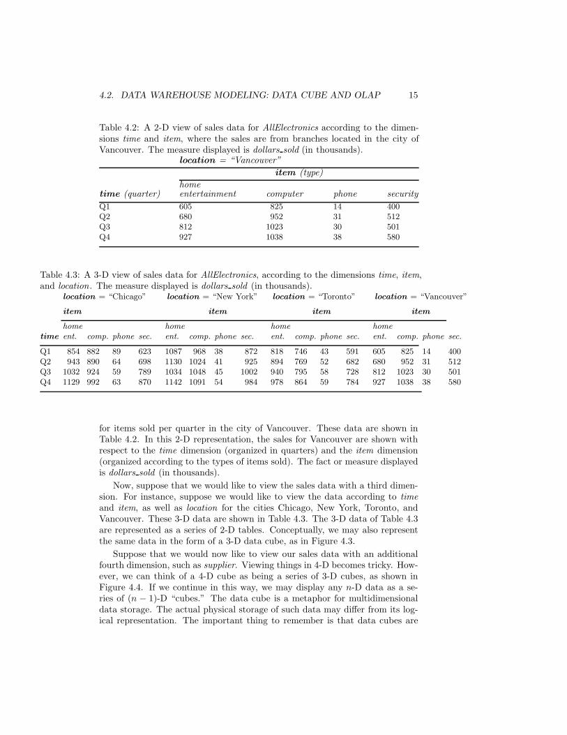
Table 4.2: A 2-D view of sales data for AllElectronics according to the dimen-sions time and item, where the sales are from branches located in the city ofVancouver. The measure displayed is dollars sold (in thousands).
location = “Vancouver”
item (type)
hometime (quarter) entertainment computer phone security
Q1 605 825 14 400Q2 680 952 31 512Q3 812 1023 30 501Q4 927 1038 38 580
Table 4.3: A 3-D view of sales data for AllElectronics, according to the dimensions time, item,and location . The measure displayed is dollars sold (in thousands).
location = “Chicago” location = “New York” location = “Toronto” location = “Vancouver”
item item item item
home home home home
time ent. comp. phone sec. ent. comp. phone sec. ent. comp. phone sec. ent. comp. phone sec.
Q1 854 882 89 623 1087 968 38 872 818 746 43 591 605 825 14 400Q2 943 890 64 698 1130 1024 41 925 894 769 52 682 680 952 31 512Q3 1032 924 59 789 1034 1048 45 1002 940 795 58 728 812 1023 30 501Q4 1129 992 63 870 1142 1091 54 984 978 864 59 784 927 1038 38 580
for items sold per quarter in the city of Vancouver. These data are shown inTable 4.2. In this 2-D representation, the sales for Vancouver are shown withrespect to the time dimension (organized in quarters) and the item dimension(organized according to the types of items sold). The fact or measure displayedis dollars sold (in thousands).
Now, suppose that we would like to view the sales data with a third dimen-sion. For instance, suppose we would like to view the data according to timeand item, as well as location for the cities Chicago, New York, Toronto, andVancouver. These 3-D data are shown in Table 4.3. The 3-D data of Table 4.3are represented as a series of 2-D tables. Conceptually, we may also representthe same data in the form of a 3-D data cube, as in Figure 4.3.
Suppose that we would now like to view our sales data with an additionalfourth dimension, such as supplier. Viewing things in 4-D becomes tricky. How-ever, we can think of a 4-D cube as being a series of 3-D cubes, as shown inFigure 4.4. If we continue in this way, we may display any n-D data as a se-ries of (n − 1)-D “cubes.” The data cube is a metaphor for multidimensionaldata storage. The actual physical storage of such data may differ from its log-ical representation. The important thing to remember is that data cubes are

16CHAPTER 4. DATA WAREHOUSING AND ONLINE ANALYTICAL PROCESSING
8181087
854
746968
882
4338
89
591872
623
698
925
789682
8701002
728
984
784
Q1
Q2
Q3
Q4
ChicagoNew York
TorontoVancouver
time
(qua
rter
s)
locati
on (c
ities)
home entertainment
computer
item (types)
phone
security
605 825 14 400
51231952680
812 1023 30 501
580381038927
Figure 4.3: A 3-D data cube representation of the data in Table 4.3, according tothe dimensions time, item, and location. The measure displayed is dollars sold(in thousands).
n-dimensional and do not confine data to 3-D.The above tables show the data at different degrees of summarization. In
the data warehousing research literature, a data cube such as each of the aboveis often referred to as a cuboid. Given a set of dimensions, we can generatea cuboid for each of the possible subsets of the given dimensions. The resultwould form a lattice of cuboids, each showing the data at a different level ofsummarization, or group by. The lattice of cuboids is then referred to as adata cube. Figure 4.5 shows a lattice of cuboids forming a data cube for thedimensions time, item, location, and supplier.
The cuboid that holds the lowest level of summarization is called the basecuboid. For example, the 4-D cuboid in Figure 4.4 is the base cuboid forthe given time, item, location, and supplier dimensions. Figure 4.3 is a 3-D(nonbase) cuboid for time, item, and location, summarized for all suppliers. The0-D cuboid, which holds the highest level of summarization, is called the apexcuboid. In our example, this is the total sales, or dollars sold, summarized overall four dimensions. The apex cuboid is typically denoted by all.
4.2.2 Stars, Snowflakes, and Fact Constellations:
Schemas for Multidimensional Data Models
The entity-relationship data model is commonly used in the design of rela-tional databases, where a database schema consists of a set of entities andthe relationships between them. Such a data model is appropriate for on-line transaction processing. A data warehouse, however, requires a concise,subject-oriented schema that facilitates online data analysis.
The most popular data model for a data warehouse is a multidimensional

4.2. DATA WAREHOUSE MODELING: DATA CUBE AND OLAP 17
605 825 14 400Q1
Q2
Q3
Q4
ChicagoNew YorkToronto
Vancouver
time
(qua
rter
s)locati
on (c
ities)
home entertainment
computer
item (types)
phonesecurity
home entertainment
computer
item (types)
phonesecurity
home entertainment
computer
item (types)
phonesecurity
supplier = “SUP1” supplier = “SUP2” supplier = “SUP3”
Figure 4.4: A 4-D data cube representation of sales data, according to the dimen-sions time, item, location, and supplier. The measure displayed is dollars sold(in thousands). For improved readability, only some of the cube values areshown.
model. Such a model can exist in the form of a star schema, a snowflakeschema, or a fact constellation schema. Let’s look at each of these schematypes.Star schema: The most common modeling paradigm is the star schema, in
which the data warehouse contains (1) a large central table (fact table)containing the bulk of the data, with no redundancy, and (2) a set ofsmaller attendant tables (dimension tables), one for each dimension.The schema graph resembles a starburst, with the dimension tables dis-played in a radial pattern around the central fact table.
Example 4.1 Star schema. A star schema for AllElectronics sales is shown in Figure 4.6.Sales are considered along four dimensions, namely, time, item, branch, and loca-tion. The schema contains a central fact table for sales that contains keys to eachof the four dimensions, along with two measures: dollars sold and units sold.To minimize the size of the fact table, dimension identifiers (such as time keyand item key) are system-generated identifiers.
Notice that in the star schema, each dimension is represented by only one ta-ble, and each table contains a set of attributes. For example, the location dimen-sion table contains the attribute set {location key, street, city, province or state,country}. This constraint may introduce some redundancy. For example, “Ur-bana” and “Chicago” are both cities in the state of Illinois, USA. Entries forsuch cities in the location dimension table will create redundancy among theattributes province or state and country, that is, (..., Urbana, IL, USA) and(..., Chicago, IL, USA). Moreover, the attributes within a dimension table mayform either a hierarchy (total order) or a lattice (partial order).
Snowflake schema: The snowflake schema is a variant of the star schemamodel, where some dimension tables are normalized, thereby further split-ting the data into additional tables. The resulting schema graph forms ashape similar to a snowflake.

18CHAPTER 4. DATA WAREHOUSING AND ONLINE ANALYTICAL PROCESSING
supplier
time, item, location, supplier
item, locationtime, location
item, suppliertime, supplier
time, location, supplier
item, location,
supplier
location,
supplier
time, item, supplier
timeitem location
time, item
time, item, location
0-D (apex) cuboid
1-D cuboids
2-D cuboids
3-D cuboids
4-D (base) cuboid
Figure 4.5: Lattice of cuboids, making up a 4-D data cube for the dimensionstime, item, location, and supplier. Each cuboid represents a different degree ofsummarization.
The major difference between the snowflake and star schema models is thatthe dimension tables of the snowflake model may be kept in normalized formto reduce redundancies. Such a table is easy to maintain and saves storagespace. However, this saving of space is negligible in comparison to the typicalmagnitude of the fact table. Furthermore, the snowflake structure can reducethe effectiveness of browsing, since more joins will be needed to execute a query.Consequently, the system performance may be adversely impacted. Hence, al-though the snowflake schema reduces redundancy, it is not as popular as thestar schema in data warehouse design.
Example 4.2 Snowflake schema. A snowflake schema for AllElectronics sales is given inFigure 4.7. Here, the sales fact table is identical to that of the star schema inFigure 4.6. The main difference between the two schemas is in the definitionof dimension tables. The single dimension table for item in the star schema isnormalized in the snowflake schema, resulting in new item and supplier tables.For example, the item dimension table now contains the attributes item key,item name, brand, type, and supplier key, where supplier key is linked to thesupplier dimension table, containing supplier key and supplier type information.Similarly, the single dimension table for location in the star schema can benormalized into two new tables: location and city. The city key in the newlocation table links to the city dimension. Notice that further normalizationcan be performed on province or state and country in the snowflake schema

4.2. DATA WAREHOUSE MODELING: DATA CUBE AND OLAP 19
time
dimension table
time_ key
day
day_of_the_week
month
quarter
year
sales
fact table
time_key
item_key
branch_key
location_key
dollars_sold
units_sold
item
dimension table
item_key
item_name
brand
type
supplier_type
branch
dimension table
branch_key
branch_name
branch_type
location
dimension table
location_key
street
city
province_or_state
country
Figure 4.6: Star schema of a data warehouse for sales.
shown in Figure 4.7, when desirable.
Fact constellation: Sophisticated applications may require multiple fact ta-bles to share dimension tables. This kind of schema can be viewed as acollection of stars, and hence is called a galaxy schema or a fact con-stellation.
Example 4.3 Fact constellation. A fact constellation schema is shown in Figure 4.8. Thisschema specifies two fact tables, sales and shipping. The sales table definitionis identical to that of the star schema (Figure 4.6). The shipping table hasfive dimensions, or keys: item key, time key, shipper key, from location, andto location, and two measures: dollars cost and units shipped. A fact constel-lation schema allows dimension tables to be shared between fact tables. Forexample, the dimensions tables for time, item, and location are shared betweenboth the sales and shipping fact tables.
In data warehousing, there is a distinction between a data warehouse and adata mart. A data warehouse collects information about subjects that span theentire organization, such as customers, items, sales, assets, and personnel, andthus its scope is enterprise-wide. For data warehouses, the fact constellationschema is commonly used, since it can model multiple, interrelated subjects. Adata mart, on the other hand, is a department subset of the data warehousethat focuses on selected subjects, and thus its scope is department-wide. For datamarts, the star or snowflake schema are commonly used, since both are gearedtoward modeling single subjects, although the star schema is more popular andefficient.

20CHAPTER 4. DATA WAREHOUSING AND ONLINE ANALYTICAL PROCESSING
time dimension table
time_key day day_of_week month quarter year
sales fact table
time_key item_key branch_key location_key dollars_sold units_sold
item dimension table
item_key item_name brand type supplier_key
branch dimension table
branch_key branch_name branch_type
location dimension table
location_key street city_key
supplier dimension table
supplier_key supplier_type
city dimension table
city_key city province_or_state country
Figure 4.7: Snowflake schema of a data warehouse for sales.
4.2.3 Dimensions: The Role of Concept Hierarchies
A concept hierarchy defines a sequence of mappings from a set of low-level con-cepts to higher-level, more general concepts. Consider a concept hierarchy for thedimension location. Cityvalues for location includeVancouver,Toronto,NewYork,andChicago. Eachcity, however, canbemapped to theprovince or state towhich itbelongs. For example,Vancouver canbemappedtoBritishColumbia, andChicagoto Illinois. The provinces and states can in turn be mapped to the country to whichthey belong, such as Canada or the USA. These mappings form a concept hier-archy for the dimension location, mapping a set of low-level concepts (i.e., cities)to higher-level, more general concepts (i.e., countries). The concept hierarchy de-scribed above is illustrated in Figure 4.9.
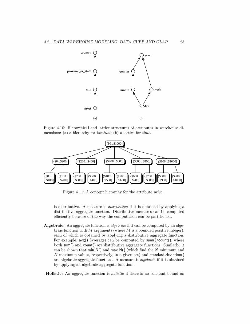
Many concept hierarchies are implicit within the database schema. For exam-ple, suppose that the dimension location is described by the attributes number,street, city, province or state, zipcode, and country. These attributes are relatedbyatotalorder, forming a concept hierarchy such as “street < city < province or state< country”. This hierarchy is shown in Figure 4.10(a). Alternatively, the at-tributes of a dimension may be organized in a partial order, forming a lattice. Anexample of a partial order for the time dimension based on the attributes day,week, month, quarter, and year is “day < {month <quarter; week} < year”.1
This lattice structure is shown in Figure 4.10(b). A concept hierarchy that is atotal or partial order among attributes in a database schema is called a schema
1Since a week often crosses the boundary of two consecutive months, it is usually nottreated as a lower abstraction of month. Instead, it is often treated as a lower abstraction ofyear, since a year contains approximately 52 weeks.

4.2. DATA WAREHOUSE MODELING: DATA CUBE AND OLAP 21
time dimension tabletime_key day day_of_week month quarter year
sales fact table
time_key item_key branch_key location_key dollars_sold units_sold
item dimension table
item_key item_name brand type supplier_type
branch dimension table
branch_key branch_name branch_type
location dimension table
location_key street city province_or_state country
shipping fact table
item_key time_key shipper_key from_location to_location dollars_cost units_shipped
shipper dimension tableshipper_key shipper_name location_key shipper_type
Figure 4.8: Fact constellation schema of a data warehouse for sales and shipping.
hierarchy. Concept hierarchies that are common to many applications may bepredefined in the data mining system, such as the concept hierarchy for time.Data mining systems should provide users with the flexibility to tailor prede-fined hierarchies according to their particular needs. For example, users maylike to define a fiscal year starting on April 1 or an academic year starting onSeptember 1.
Concept hierarchies may also be defined by discretizing or grouping valuesfor a given dimension or attribute, resulting in a set-grouping hierarchy. Atotal or partial order can be defined among groups of values. An example of aset-grouping hierarchy is shown in Figure 4.11 for the dimension price, wherean interval ($X . . . $Y ] denotes the range from $X (exclusive) to $Y (inclusive).
There may be more than one concept hierarchy for a given attribute ordimension, based on different user viewpoints. For instance, a user may pre-fer to organize price by defining ranges for inexpensive, moderately priced, andexpensive.
Concept hierarchies may be provided manually by system users, domainexperts, or knowledge engineers, or may be automatically generated based onstatistical analysis of the data distribution. The automatic generation of concepthierarchies is discussed in Chapter 3 as a preprocessing step in preparation fordata mining.
Concept hierarchies allow data to be handled at varying levels of abstraction,as we shall see in the following subsection.

22CHAPTER 4. DATA WAREHOUSING AND ONLINE ANALYTICAL PROCESSING
Canada
British Columbia Ontario
Vancouver Victoria OttawaToronto Chicago UrbanaBuffalo
New York
New York
Illinois
USA
location
country
city
province_or_state
Figure 4.9: A concept hierarchy for the dimension location. Due to space limi-tations, not all of the nodes of the hierarchy are shown (as indicated by the useof “ellipsis” between nodes).
4.2.4 Measures: Their Categorization and Computation
“How are measures computed?” To answer this question, we first study howmeasures can be categorized. Note that a multidimensional point in the datacube space can be defined by a set of dimension-value pairs, for example, 〈time= “Q1”, location = “Vancouver”, item = “computer”〉. A data cube measureis a numerical function that can be evaluated at each point in the data cubespace. A measure value is computed for a given point by aggregating the datacorresponding to the respective dimension-value pairs defining the given point.We will look at concrete examples of this shortly.
Measures can be organized into three categories (i.e., distributive, algebraic,holistic), based on the kind of aggregate functions used.
Distributive: An aggregate function is distributive if it can be computed ina distributed manner as follows. Suppose the data are partitioned inton sets. We apply the function to each partition, resulting in n aggregatevalues. If the result derived by applying the function to the n aggregatevalues is the same as that derived by applying the function to the entiredata set (without partitioning), the function can be computed in a dis-tributed manner. For example, sum() can be computed for a data cubeby first partitioning the cube into a set of subcubes, computing sum() foreach subcube, and then summing up the counts obtained for each sub-cube. Hence, sum() is a distributive aggregate function. For the samereason, count(), min(), and max() are distributive aggregate functions.By treating the count value of each nonempty base cell as 1 by default,count() of any cell in a cube can be viewed as the sum of the count val-ues of all of its corresponding child cells in its subcube. Thus, count()
4.2. DATA WAREHOUSE MODELING: DATA CUBE AND OLAP 23
country
city
province_or_state
month week
year
day
quarter
street
(a) (b)
Figure 4.10: Hierarchical and lattice structures of attributes in warehouse di-mensions: (a) a hierarchy for location; (b) a lattice for time.
($0 $1000]
($800 $1000]
($0 … �$100]
($100… $200]
($800… $900]
($900… $1000]
($600… $700]
($700… $800]
($200… $300]
($300… $400]
($400… $500]
($500… $600]
($600 $800]($400 $600]($200 $400]($0 $200]
Figure 4.11: A concept hierarchy for the attribute price.
is distributive. A measure is distributive if it is obtained by applying adistributive aggregate function. Distributive measures can be computedefficiently because of the way the computation can be partitioned.
Algebraic: An aggregate function is algebraic if it can be computed by an alge-braic function with M arguments (where M is a bounded positive integer),each of which is obtained by applying a distributive aggregate function.For example, avg() (average) can be computed by sum()/count(), whereboth sum() and count() are distributive aggregate functions. Similarly, itcan be shown that min N() and max N() (which find the N minimum andN maximum values, respectively, in a given set) and standard deviation()are algebraic aggregate functions. A measure is algebraic if it is obtainedby applying an algebraic aggregate function.
Holistic: An aggregate function is holistic if there is no constant bound on

24CHAPTER 4. DATA WAREHOUSING AND ONLINE ANALYTICAL PROCESSING
the storage size needed to describe a subaggregate. That is, there does notexist an algebraic function with M arguments (where M is a constant) thatcharacterizes the computation. Common examples of holistic functionsinclude median(), mode(), and rank(). A measure is holistic if it is obtainedby applying a holistic aggregate function.
Most large data cube applications require efficient computation of distribu-tive and algebraic measures. Many efficient techniques for this exist. In contrast,it is difficult to compute holistic measures efficiently. Efficient techniques to ap-proximate the computation of some holistic measures, however, do exist. Forexample, rather than computing the exact median(), Equation (2.3) of Chap-ter 2 can be used to estimate the approximate median value for a large dataset. In many cases, such techniques are sufficient to overcome the difficulties ofefficient computation of holistic measures.
Various methods for computing different measures in the construction ofdata cubes are discussed in-depth in Chapter 5. Notice that most of the cur-rent data cube technology confines the measures of multidimensional databasesto numerical data. However, measures can also be applied to other kinds ofdata, such as spatial, multimedia, or text data. Modeling and computing suchmeasures will be discussed in Volume 2.
4.2.5 Typical OLAP Operations
“How are concept hierarchies useful in OLAP?” In the multidimensional model,data are organized into multiple dimensions, and each dimension contains mul-tiple levels of abstraction defined by concept hierarchies. This organizationprovides users with the flexibility to view data from different perspectives. Anumber of OLAP data cube operations exist to materialize these different views,allowing interactive querying and analysis of the data at hand. Hence, OLAPprovides a user-friendly environment for interactive data analysis.
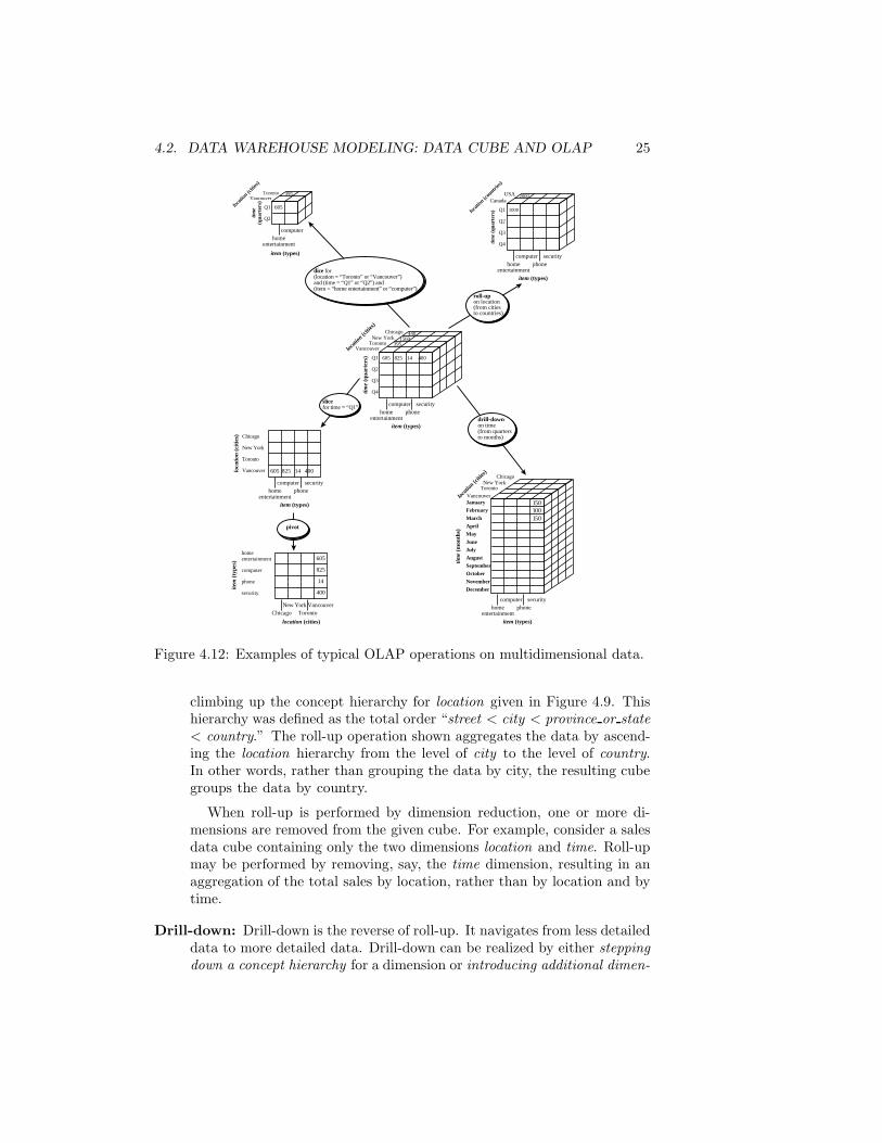
Example 4.4 OLAP operations. Let’s look at some typical OLAP operations for mul-tidimensional data. Each of the operations described below is illustrated inFigure 4.12. At the center of the figure is a data cube for AllElectronics sales.The cube contains the dimensions location, time, and item, where location is ag-gregated with respect to city values, time is aggregated with respect to quarters,and item is aggregated with respect to item types. To aid in our explanation,we refer to this cube as the central cube. The measure displayed is dollars sold(in thousands). (For improved readability, only some of the cubes’ cell valuesare shown.) The data examined are for the cities Chicago, New York, Toronto,and Vancouver.
Roll-up: The roll-up operation (also called the drill-up operation by somevendors) performs aggregation on a data cube, either by climbing up aconcept hierarchy for a dimension or by dimension reduction. Figure 4.12shows the result of a roll-up operation performed on the central cube by
4.2. DATA WAREHOUSE MODELING: DATA CUBE AND OLAP 25
Q1
Q2
Q3
Q4
1000
Canada USA 2000
time
(qua
rter
s)
locati
on (c
ountri
es)
home entertainment
computer
item (types)
phone security
Toronto 395
Q1
Q2
605
Vancouver
time
(qua
rter
s)
locati
on (c
ities)
home entertainment
computer
item (types)
January
February
March
April
May
June
July
August
September
October
November
December
Chicago New York
Toronto
Vancouver
time
(mon
ths)
locati
on (c
ities)
home entertainment
computer
item (types)
phone security
150 100 150
605 825 14 400 Q1
Q2
Q3
Q4
Chicago New York
Toronto Vancouver
time
(qua
rter
s)
locati
on (c
ities)
home entertainment
computer
item (types)
phone security
440
395 1560
dice for (location = “Toronto” or “Vancouver”) and (time = “Q1” or “Q2”) and (item = “home entertainment” or “computer”)
roll-up on location (from cities to countries)
slice for time = “Q1”
Chicago
New York
Toronto
Vancouver
home entertainment
computer
item (types)
phone security
loca
tion
(cit
ies)
605 825 14 400
home entertainment
computer
phone
security
605
825
14
400
Chicago New York
location (cities)
item
(ty
pes)
Toronto Vancouver
pivot
drill-down on time (from quarters to months)
Figure 4.12: Examples of typical OLAP operations on multidimensional data.
climbing up the concept hierarchy for location given in Figure 4.9. Thishierarchy was defined as the total order “street < city < province or state< country.” The roll-up operation shown aggregates the data by ascend-ing the location hierarchy from the level of city to the level of country.In other words, rather than grouping the data by city, the resulting cubegroups the data by country.
When roll-up is performed by dimension reduction, one or more di-mensions are removed from the given cube. For example, consider a salesdata cube containing only the two dimensions location and time. Roll-upmay be performed by removing, say, the time dimension, resulting in anaggregation of the total sales by location, rather than by location and bytime.
Drill-down: Drill-down is the reverse of roll-up. It navigates from less detaileddata to more detailed data. Drill-down can be realized by either steppingdown a concept hierarchy for a dimension or introducing additional dimen-

26CHAPTER 4. DATA WAREHOUSING AND ONLINE ANALYTICAL PROCESSING
sions. Figure 4.12 shows the result of a drill-down operation performedon the central cube by stepping down a concept hierarchy for time definedas “day < month < quarter < year.” Drill-down occurs by descendingthe time hierarchy from the level of quarter to the more detailed level ofmonth. The resulting data cube details the total sales per month ratherthan summarizing them by quarter.
Because a drill-down adds more detail to the given data, it can also beperformed by adding new dimensions to a cube. For example, a drill-downon the central cube of Figure 4.12 can occur by introducing an additionaldimension, such as customer group.
Slice and dice: The slice operation performs a selection on one dimension ofthe given cube, resulting in a subcube. Figure 4.12 shows a slice operationwhere the sales data are selected from the central cube for the dimensiontime using the criterion time = “Q1”. The dice operation defines a sub-cube by performing a selection on two or more dimensions. Figure 4.12shows a dice operation on the central cube based on the following selectioncriteria that involve three dimensions: (location = “Toronto” or “Vancou-ver”) and (time = “Q1” or “Q2”) and (item = “home entertainment” or“computer”).
Pivot (rotate): Pivot (also called rotate) is a visualization operation that ro-tates the data axes in view in order to provide an alternative presentationof the data. Figure 4.12 shows a pivot operation where the item and loca-tion axes in a 2-D slice are rotated. Other examples include rotating theaxes in a 3-D cube, or transforming a 3-D cube into a series of 2-D planes.
Other OLAP operations: Some OLAP systems offer additional drilling op-erations. For example, drill-across executes queries involving (i.e., across)more than one fact table. The drill-through operation uses relationalSQL facilities to drill through the bottom level of a data cube down to itsback-end relational tables.
Other OLAP operations may include ranking the top N or bottomN items in lists, as well as computing moving averages, growth rates,interests, internal rates of return, depreciation, currency conversions, andstatistical functions.
OLAP offers analytical modeling capabilities, including a calculation enginefor deriving ratios, variance, and so on, and for computing measures across mul-tiple dimensions. It can generate summarizations, aggregations, and hierarchiesat each granularity level and at every dimension intersection. OLAP also sup-ports functional models for forecasting, trend analysis, and statistical analysis.In this context, an OLAP engine is a powerful data analysis tool.

4.3. DATA WAREHOUSE DESIGN AND USAGE 27
OLAP Systems versus Statistical Databases
Many of the characteristics of OLAP systems, such as the use of a multidi-mensional data model and concept hierarchies, the association of measures withdimensions, and the notions of roll-up and drill-down, also exist in earlier workon statistical databases (SDBs). A statistical database is a database systemthat is designed to support statistical applications. Similarities between the twotypes of systems are rarely discussed, mainly due to differences in terminologyand application domains.
OLAP and SDB systems, however, have distinguishing differences. WhileSDBs tend to focus on socioeconomic applications, OLAP has been targeted forbusiness applications. Privacy issues regarding concept hierarchies are a majorconcern for SDBs. For example, given summarized socioeconomic data, it iscontroversial to allow users to view the corresponding low-level data. Finally,unlike SDBs, OLAP systems are designed for handling huge amounts of dataefficiently.
4.2.6 A Starnet Query Model for Querying
Multidimensional Databases
The querying of multidimensional databases can be based on a starnet model.A starnet model consists of radial lines emanating from a central point, whereeach line represents a concept hierarchy for a dimension. Each abstraction levelin the hierarchy is called a footprint. These represent the granularities availablefor use by OLAP operations such as drill-down and roll-up.
Example 4.5 Starnet. A starnet query model for the AllElectronics data warehouse is shownin Figure 4.13. This starnet consists of four radial lines, representing concepthierarchies for the dimensions location, customer, item, and time, respectively.Each line consists of footprints representing abstraction levels of the dimension.For example, the time line has four footprints: “day,” “month,” “quarter,” and“year.” A concept hierarchy may involve a single attribute (like date for the timehierarchy) or several attributes (e.g., the concept hierarchy for location involvesthe attributes street, city, province or state, and country). In order to examinethe item sales at AllElectronics, users can roll up along the time dimension frommonth to quarter, or, say, drill down along the location dimension from countryto city. Concept hierarchies can be used to generalize data by replacing low-level values (such as “day” for the time dimension) by higher-level abstractions(such as “year”), or to specialize data by replacing higher-level abstractionswith lower-level values.
4.3 Data Warehouse Design and Usage
“What goes into the design of a data warehouse? How are data warehousesused? How do data warehousing and OLAP relate to data mining?” This sec-tion tackles these questions. We study the design and usage of data warehousing

28CHAPTER 4. DATA WAREHOUSING AND ONLINE ANALYTICAL PROCESSING
continent
country
province_or_state
city
street
name brand category type
name
category
group
year
quarter
month
day
time
item
locationcustomer
Figure 4.13: Modeling business queries: a starnet model.
for information processing, analytical processing, and data mining. We beginby presenting a business analysis framework for data warehouse design (Sec-tion 4.3.1). Section 4.3.2 looks at the design process, while Section 4.3.3 studiesdata warehouse usage. Finally, Section 4.3.4 describes multidimensional datamining a powerful paradigm that integrates OLAP with data mining technol-ogy.
4.3.1 A Business Analysis Framework for Data Warehouse
Design
“What can business analysts gain from having a data warehouse?” First, havinga data warehouse may provide a competitive advantage by presenting relevantinformation from which to measure performance and make critical adjustmentsin order to help win over competitors. Second, a data warehouse can enhancebusiness productivity because it is able to quickly and efficiently gather infor-mation that accurately describes the organization. Third, a data warehousefacilitates customer relationship management because it provides a consistentview of customers and items across all lines of business, all departments, and allmarkets. Finally, a data warehouse may bring about cost reduction by trackingtrends, patterns, and exceptions over long periods in a consistent and reliablemanner.
To design an effective data warehouse we need to understand and analyzebusiness needs and construct a business analysis framework. The construction

4.3. DATA WAREHOUSE DESIGN AND USAGE 29
of a large and complex information system can be viewed as the construction ofa large and complex building, for which the owner, architect, and builder havedifferent views. These views are combined to form a complex framework thatrepresents the top-down, business-driven, or owner’s perspective, as well as thebottom-up, builder-driven, or implementor’s view of the information system.
Four different views regarding the design of a data warehouse must be con-sidered: the top-down view, the data source view, the data warehouse view, andthe business query view.
• The top-down view allows the selection of the relevant information nec-essary for the data warehouse. This information matches the current andfuture business needs.
• The data source view exposes the information being captured, stored,and managed by operational systems. This information may be doc-umented at various levels of detail and accuracy, from individual datasource tables to integrated data source tables. Data sources are oftenmodeled by traditional data modeling techniques, such as the entity-relationship model or CASE (computer-aided software engineering) tools.
• The data warehouse view includes fact tables and dimension tables.It represents the information that is stored inside the data warehouse,including precalculated totals and counts, as well as information regardingthe source, date, and time of origin, added to provide historical context.
• Finally, the business query view is the perspective of data in the datawarehouse from the viewpoint of the end user.
Building and using a data warehouse is a complex task because it requiresbusiness skills, technology skills, and program management skills. Regardingbusiness skills, building a data warehouse involves understanding how such sys-tems store and manage their data, how to build extractors that transfer datafrom the operational system to the data warehouse, and how to build ware-house refresh software that keeps the data warehouse reasonably up-to-datewith the operational system’s data. Using a data warehouse involves under-standing the significance of the data it contains, as well as understanding andtranslating the business requirements into queries that can be satisfied by thedata warehouse. Regarding technology skills, data analysts are required to un-derstand how to make assessments from quantitative information and derivefacts based on conclusions from historical information in the data warehouse.These skills include the ability to discover patterns and trends, to extrapolatetrends based on history and look for anomalies or paradigm shifts, and to presentcoherent managerial recommendations based on such analysis. Finally, programmanagement skills involve the need to interface with many technologies, ven-dors, and end users in order to deliver results in a timely and cost-effectivemanner.

30CHAPTER 4. DATA WAREHOUSING AND ONLINE ANALYTICAL PROCESSING
4.3.2 The Data Warehouse Design Process
Let’s look at various approaches to the process of data warehouse design andthe steps involved.
A data warehouse can be built using a top-down approach, a bottom-upapproach, or a combination of both. The top-down approach starts with theoverall design and planning. It is useful in cases where the technology is matureand well known, and where the business problems that must be solved are clearand well understood. The bottom-up approach starts with experiments andprototypes. This is useful in the early stage of business modeling and technologydevelopment. It allows an organization to move forward at considerably lessexpense and to evaluate the benefits of the technology before making significantcommitments. In the combined approach, an organization can exploit theplanned and strategic nature of the top-down approach while retaining the rapidimplementation and opportunistic application of the bottom-up approach.
From the software engineering point of view, the design and construction of adata warehouse may consist of the following steps: planning, requirements study,problem analysis, warehouse design, data integration and testing, and finally de-ploymentof thedatawarehouse. Large software systemscanbedevelopedusing twomethodologies: thewaterfallmethod or the spiralmethod. Thewaterfallmethodperforms a structured and systematic analysis at each step before proceeding tothe next, which is like a waterfall, falling from one step to the next. The spiralmethod involves the rapid generation of increasingly functional systems, withshort intervals between successive releases. This is considered a good choice fordata warehouse development, especially for data marts, because the turnaroundtime is short, modifications can be done quickly, and new designs and technologiescan be adapted in a timely manner.
In general, the warehouse design process consists of the following steps:
1. Choose a business process to model, for example, orders, invoices, ship-ments, inventory, account administration, sales, or the general ledger. Ifthe business process is organizational and involves multiple complex ob-ject collections, a data warehouse model should be followed. However, ifthe process is departmental and focuses on the analysis of one kind ofbusiness process, a data mart model should be chosen.
2. Choose the grain of the business process. The grain is the fundamental,atomic level of data to be represented in the fact table for this process, forexample, individual transactions, individual daily snapshots, and so on.
3. Choose the dimensions that will apply to each fact table record. Typi-cal dimensions are time, item, customer, supplier, warehouse, transactiontype, and status.
4. Choose the measures that will populate each fact table record. Typicalmeasures are numeric additive quantities like dollars sold and units sold.
Because data warehouse construction is a difficult and long-term task, itsimplementation scope should be clearly defined. The goals of an initial data

4.3. DATA WAREHOUSE DESIGN AND USAGE 31
warehouse implementation should be specific, achievable, and measurable. Thisinvolves determining the time and budget allocations, the subset of the orga-nization that is to be modeled, the number of data sources selected, and thenumber and types of departments to be served.
Once a data warehouse is designed and constructed, the initial deployment ofthe warehouse includes initial installation, roll-out planning, training, and ori-entation. Platform upgrades and maintenance must also be considered. Datawarehouse administration includes data refreshment, data source synchroniza-tion, planning for disaster recovery, managing access control and security, man-aging data growth, managing database performance, and data warehouse en-hancement and extension. Scope management includes controlling the numberand range of queries, dimensions, and reports; limiting the size of the datawarehouse; or limiting the schedule, budget, or resources.
Various kinds of data warehouse design tools are available. Data warehousedevelopment tools provide functions to define and edit metadata repositorycontents (such as schemas, scripts, or rules), answer queries, output reports,and ship metadata to and from relational database system catalogues. Plan-ning and analysis tools study the impact of schema changes and of refreshperformance when changing refresh rates or time windows.
4.3.3 Data Warehouse Usage for Information Processing
Data warehouses and data marts are used in a wide range of applications.Business executives use the data in data warehouses and data marts to performdata analysis and make strategic decisions. In many firms, data warehousesare used as an integral part of a plan-execute-assess “closed-loop” feedbacksystem for enterprise management. Data warehouses are used extensively inbanking and financial services, consumer goods and retail distribution sectors,and controlled manufacturing, such as demand-based production.
Typically, the longer a data warehouse has been in use, the more it will haveevolved. This evolution takes place throughout a number of phases. Initially, thedata warehouse is mainly used for generating reports and answering predefinedqueries. Progressively, it is used to analyze summarized and detailed data, wherethe results are presented in the form of reports and charts. Later, the datawarehouse is used for strategic purposes, performing multidimensional analysisand sophisticated slice-and-dice operations. Finally, the data warehouse maybe employed for knowledge discovery and strategic decision making using datamining tools. In this context, the tools for data warehousing can be categorizedinto access and retrieval tools, database reporting tools, data analysis tools, anddata mining tools.
Business users need to have the means to know what exists in the data ware-house (through metadata), how to access the contents of the data warehouse,how to examine the contents using analysis tools, and how to present the resultsof such analysis.
There are three kinds of data warehouse applications: information process-ing, analytical processing, and data mining:

32CHAPTER 4. DATA WAREHOUSING AND ONLINE ANALYTICAL PROCESSING
• Information processing supports querying, basic statistical analysis,and reporting using crosstabs, tables, charts, or graphs. A current trendin data warehouse information processing is to construct low-cost Web-based accessing tools that are then integrated with Web browsers.
• Analytical processing supports basic OLAP operations, including slice-and-dice, drill-down, roll-up, and pivoting. It generally operates on his-torical data in both summarized and detailed forms. The major strengthof online analytical processing over information processing is the multidi-mensional data analysis of data warehouse data.
• Data mining supports knowledge discovery by finding hidden patternsand associations, constructing analytical models, performing classificationand prediction, and presenting the mining results using visualization tools.
“How does data mining relate to information processing and online analyticalprocessing?” Information processing, based on queries, can find useful informa-tion. However, answers to such queries reflect the information directly storedin databases or computable by aggregate functions. They do not reflect sophis-ticated patterns or regularities buried in the database. Therefore, informationprocessing is not data mining.
Online analytical processing comes a step closer to data mining because it canderive information summarized at multiple granularities from user-specified sub-sets of a data warehouse. Such descriptions are equivalent to the class/conceptdescriptions discussed in Chapter 1. Because data mining systems can alsomine generalized class/concept descriptions, this raises some interesting ques-tions: “Do OLAP systems perform data mining? Are OLAP systems actuallydata mining systems?”
The functionalities of OLAP and data mining can be viewed as disjoint:OLAP is a data summarization/aggregation tool that helps simplify data anal-ysis, while data mining allows the automated discovery of implicit patterns andinteresting knowledge hidden in large amounts of data. OLAP tools are tar-geted toward simplifying and supporting interactive data analysis, whereas thegoal of data mining tools is to automate as much of the process as possible,while still allowing users to guide the process. In this sense, data mining goesone step beyond traditional online analytical processing.
An alternative and broader view of data mining may be adopted in whichdata mining covers both data description and data modeling. Because OLAPsystems can present general descriptions of data from data warehouses, OLAPfunctions are essentially for user-directed data summarization and comparison(by drilling, pivoting, slicing, dicing, and other operations). These are, thoughlimited, data mining functionalities. Yet according to this view, data min-ing covers a much broader spectrum than simple OLAP operations because itperforms not only data summarization and comparison but also association,classification, prediction, clustering, time-series analysis, and other data analy-sis tasks.

4.3. DATA WAREHOUSE DESIGN AND USAGE 33
Data mining is not confined to the analysis of data stored in data warehouses.It may analyze data existing at more detailed granularities than the summa-rized data provided in a data warehouse. It may also analyze transactional,spatial, textual, and multimedia data that are difficult to model with currentmultidimensional database technology. In this context, data mining covers abroader spectrum than OLAP with respect to data mining functionality andthe complexity of the data handled.
Because data mining involves more automated and deeper analysis thanOLAP, data mining is expected to have broader applications. Data miningcan help business managers find and reach more suitable customers, as wellas gain critical business insights that may help drive market share and raiseprofits. In addition, data mining can help managers understand customergroup characteristics and develop optimal pricing strategies accordingly, cor-rect item bundling based not on intuition but on actual item groups derivedfrom customer purchase patterns, reduce promotional spending, and at thesame time increase the overall net effectiveness of promotions.
4.3.4 From Online Analytical Processing to
Multidimensional Data Mining
The field of data mining has conducted substantial research regarding miningon various types of data, including relational data, data from data warehouses,transaction data, time-series data, spatial data, text data, and flat files. Multi-dimensional data mining (also known as exploratory multidimensional datamining, online analytical mining, or OLAM) integrates online analyticalprocessing (OLAP) with data mining to uncover knowledge in multidimen-sional databases. Among the many different paradigms and architectures ofdata mining systems, multidimensional data mining is particularly importantfor the following reasons:
• High quality of data in data warehouses: Most data mining toolsneed to work on integrated, consistent, and cleaned data, which requirescostly data cleaning, data integration, and data transformation as pre-processing steps. A data warehouse constructed by such preprocessingserves as a valuable source of high-quality data for OLAP as well as fordata mining. Notice that data mining may also serve as a valuable toolfor data cleaning and data integration as well.
• Available information processing infrastructure surrounding datawarehouses: Comprehensive information processing and data analysisinfrastructures have been or will be systematically constructed surround-ing data warehouses, which include accessing, integration, consolidation,and transformation of multiple heterogeneous databases, ODBC/OLEDB connections, Web-accessing and service facilities, and reporting andOLAP analysis tools. It is prudent to make the best use of the availableinfrastructures rather than constructing everything from scratch.

34CHAPTER 4. DATA WAREHOUSING AND ONLINE ANALYTICAL PROCESSING
• OLAP-based exploration of multidimensional data: Effective datamining needs exploratory data analysis. A user will often want totraverse through a database, select portions of relevant data, analyzethem at different granularities, and present knowledge/results in differ-ent forms. Multidimensional data mining provides facilities for mining ondifferent subsets of data and at varying levels of abstraction, by drilling,pivoting, filtering, dicing, and slicing on a data cube and/or intermediatedata mining results. This, together with data/knowledge visualizationtools, greatly enhance the power and flexibility of data mining.
• Online selection of data mining functions: Users may not alwaysknow the specific kinds of knowledge they would like to mine. Byintegrating OLAP with various data mining functions, multidimensionaldata mining provides users with the flexibility to select desired datamining functions and swap data mining tasks dynamically.
Chapter 5 describe data warehouses on a finer level by exploring implementationissues such as data cube computation, OLAP query answering strategies, andmultidimensional data mining. The chapters following it are devoted to thestudy of data mining techniques. As we have seen, the introduction to datawarehousing and OLAP technology presented in this chapter is essential to ourstudy of data mining. This is because data warehousing provides users withlarge amounts of clean, organized, and summarized data, which greatly facili-tates data mining. For example, rather than storing the details of each salestransaction, a data warehouse may store a summary of the transactions peritem type for each branch or, summarized to a higher level, for each country.The capability of OLAP to provide multiple and dynamic views of summarizeddata in a data warehouse sets a solid foundation for successful data mining.
Moreover,wealsobelievethatdataminingshouldbeahuman-centeredprocess.Rather thanasking adatamining systemtogeneratepatterns andknowledgeauto-matically, a user will often need to interactwith the system to perform exploratorydataanalysis. OLAPsetsagoodexample for interactivedataanalysis andprovidesthe necessary preparations for exploratory data mining. Consider the discovery ofassociation patterns, for example. Instead of mining associations at a primitive(i.e., low) data level among transactions, users should be allowed to specify roll-upoperations along any dimension. For example, a user may like to roll up on the itemdimension to go from viewing the data for particular TV sets that were purchasedto viewing the brands of these TVs, such as SONY or Toshiba. Users may alsonavigate from the transaction level to the customer level or customer-type levelin the search for interesting associations. Such an OLAP-style of data mining ischaracteristic of multidimensional data mining. In our study of the principles ofdata mining in this book, we place particular emphasis on multidimensional datamining, that is, on the integration of data mining and OLAP technology.

4.4. DATA WAREHOUSE IMPLEMENTATION 35
4.4 Data Warehouse Implementation
Data warehouses contain huge volumes of data. OLAP servers demand thatdecision support queries be answered in the order of seconds. Therefore, itis crucial for data warehouse systems to support highly efficient cube compu-tation techniques, access methods, and query processing techniques. In thissection, we present an overview of methods for the efficient implementation ofdata warehouse systems. Section 4.4.1 explores how to compute data cubesefficiently. Section 4.4.2 shows how OLAP data can be indexed, using eitherbitmap or join indices. Next, we study how OLAP queries are processed (Sec-tion 4.4.3). Finally, Section 4.4.4 presents various types of warehouse serversfor OLAP processing.
4.4.1 Efficient Data Cube Computation: An Overview
At the core of multidimensional data analysis is the efficient computation ofaggregations across many sets of dimensions. In SQL terms, these aggregationsare referred to as group-by’s. Each group-by can be represented by a cuboid,where the set of group-by’s forms a lattice of cuboids defining a data cube.In this section, we explore issues relating to the efficient computation of datacubes.
The compute cube Operator and the Curse of Dimensionality
One approach to cube computation extends SQL so as to include a computecube operator. The compute cube operator computes aggregates over all subsetsof the dimensions specified in the operation. This can require excessive storagespace, especially for large numbers of dimensions. We start with an intuitivelook at what is involved in the efficient computation of data cubes.
Example 4.6 A data cube is a lattice of cuboids. Suppose that you would like to createa data cube for AllElectronics sales that contains the following: city, item,year, and sales in dollars. You would like to be able to analyze the data, withqueries such as the following:
• “Compute the sum of sales, grouping by city and item.”
• “Compute the sum of sales, grouping by city.”
• “Compute the sum of sales, grouping by item.”
What is the total number of cuboids, or group-by’s, that can be computedfor this data cube? Taking the three attributes, city, item, and year, as thedimensions for the data cube, and sales in dollars as the measure, the totalnumber of cuboids, or group-by’s, that can be computed for this data cube is23 = 8. The possible group-by’s are the following: {(city, item, year), (city,item), (city, year), (item, year), (city), (item), (year), ()}, where () means thatthe group-by is empty (i.e., the dimensions are not grouped). These group-by’sform a lattice of cuboids for the data cube, as shown in Figure 4.14. The base

36CHAPTER 4. DATA WAREHOUSING AND ONLINE ANALYTICAL PROCESSING
cuboid contains all three dimensions, city, item, and year. It can return thetotal sales for any combination of the three dimensions. The apex cuboid,or 0-D cuboid, refers to the case where the group-by is empty. It contains thetotal sum of all sales. The base cuboid is the least generalized (most specific)of the cuboids. The apex cuboid is the most generalized (least specific) of thecuboids, and is often denoted as all. If we start at the apex cuboid and exploredownward in the lattice, this is equivalent to drilling down within the datacube. If we start at the base cuboid and explore upward, this is akin to rollingup.
An SQL query containing no group-by, such as “compute the sum of totalsales,” is a zero-dimensional operation. An SQL query containing one group-by, such as “compute the sum of sales, group by city,” is a one-dimensionaloperation. A cube operator on n dimensions is equivalent to a collection ofgroup by statements, one for each subset of the n dimensions. Therefore, thecube operator is the n-dimensional generalization of the group by operator.
Similar to the syntax of SQL, the data cube in Example 4.1 could be de-fined as
define cube sales cube [city, item, year]: sum(sales in dollars)
For a cube with n dimensions, there are a total of 2n cuboids, including thebase cuboid. A statement such as
compute cube sales cube
would explicitly instruct the system to compute the sales aggregate cuboidsfor all of the eight subsets of the set {city, item, year}, including the emptysubset. A cube computation operator was first proposed and studied by Grayet al. [GCB+97].
Online analytical processing may need to access different cuboids for dif-ferent queries. Therefore, it may seem like a good idea to compute all or atleast some of the cuboids in a data cube in advance. Precomputation leads tofast response time and avoids some redundant computation. Most, if not all,OLAP products resort to some degree of precomputation of multidimensionalaggregates.
(item) (year)(city)
()
(item, year)
(city, item, year)
(city, item) (city, year)
O-D (apex) cuboid
1-D cuboids
2-D cuboids
3-D (base) cuboid
Figure 4.14: Lattice of cuboids, making up a 3-D data cube. Each cuboidrepresents a different group-by. The base cuboid contains the three dimensionscity, item, and year.
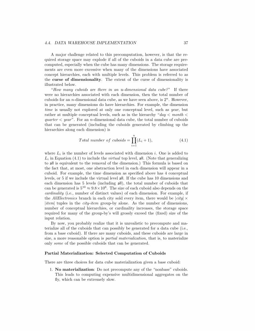
4.4. DATA WAREHOUSE IMPLEMENTATION 37
A major challenge related to this precomputation, however, is that the re-quired storage space may explode if all of the cuboids in a data cube are pre-computed, especially when the cube has many dimensions. The storage require-ments are even more excessive when many of the dimensions have associatedconcept hierarchies, each with multiple levels. This problem is referred to asthe curse of dimensionality. The extent of the curse of dimensionality isillustrated below.
“How many cuboids are there in an n-dimensional data cube?” If therewere no hierarchies associated with each dimension, then the total number ofcuboids for an n-dimensional data cube, as we have seen above, is 2n. However,in practice, many dimensions do have hierarchies. For example, the dimensiontime is usually not explored at only one conceptual level, such as year, butrather at multiple conceptual levels, such as in the hierarchy “day < month <
quarter < year”. For an n-dimensional data cube, the total number of cuboidsthat can be generated (including the cuboids generated by climbing up thehierarchies along each dimension) is
Total number of cuboids =n∏
i=1
(Li + 1), (4.1)
where Li is the number of levels associated with dimension i. One is added toLi in Equation (4.1) to include the virtual top level, all. (Note that generalizingto all is equivalent to the removal of the dimension.) This formula is based onthe fact that, at most, one abstraction level in each dimension will appear in acuboid. For example, the time dimension as specified above has 4 conceptuallevels, or 5 if we include the virtual level all. If the cube has 10 dimensions andeach dimension has 5 levels (including all), the total number of cuboids thatcan be generated is 510 ≈ 9.8×10⁶. The size of each cuboid also depends on thecardinality (i.e., number of distinct values) of each dimension. For example, ifthe AllElectronics branch in each city sold every item, there would be |city| ×|item| tuples in the city-item group-by alone. As the number of dimensions,number of conceptual hierarchies, or cardinality increases, the storage spacerequired for many of the group-by’s will grossly exceed the (fixed) size of theinput relation.
By now, you probably realize that it is unrealistic to precompute and ma-terialize all of the cuboids that can possibly be generated for a data cube (i.e.,from a base cuboid). If there are many cuboids, and these cuboids are large insize, a more reasonable option is partial materialization, that is, to materializeonly some of the possible cuboids that can be generated.
Partial Materialization: Selected Computation of Cuboids
There are three choices for data cube materialization given a base cuboid:
1. No materialization: Do not precompute any of the “nonbase” cuboids.This leads to computing expensive multidimensional aggregates on thefly, which can be extremely slow.
38CHAPTER 4. DATA WAREHOUSING AND ONLINE ANALYTICAL PROCESSING
2. Full materialization: Precompute all of the cuboids. The resultinglattice of computed cuboids is referred to as the full cube. This choicetypically requires huge amounts of memory space in order to store all ofthe precomputed cuboids.
3. Partial materialization: Selectively compute aproper subset of thewholeset of possible cuboids. Alternatively, we may compute a subset of the cube,which contains only those cells that satisfy someuser-specified criterion, suchas where the tuple count of each cell is above some threshold. We will use theterm subcube to refer to the latter case, where only some of the cells may beprecomputed for various cuboids. Partialmaterialization represents an inter-esting trade-off between storage space and response time.
The partial materialization of cuboids or subcubes should consider threefactors: (1) identify the subset of cuboids or subcubes to materialize; (2) exploitthe materialized cuboids or subcubes during query processing; and (3) efficientlyupdate the materialized cuboids or subcubes during load and refresh.
Theselectionofthesubsetofcuboidsor subcubestomaterialize shouldtake intoaccount the queries in the workload, their frequencies, and their accessing costs. Inaddition, it should consider workload characteristics, the cost for incremental up-dates, and the total storage requirements. The selection must also consider thebroad context of physical database design, such as the generation and selection ofindices. SeveralOLAPproducts have adoptedheuristic approaches for cuboid andsubcube selection. Apopular approach is tomaterialize the set of cuboids onwhichother frequently referenced cuboids are based. Alternatively, we can compute aniceberg cube, which is a data cube that stores only those cube cells whose aggre-gate value (e.g., count) is above some minimum support threshold. Another com-mon strategy is tomaterialize a shell cube. This involves precomputing the cuboidsfor only a small number of dimensions (such as 3 to 5) of a data cube. Queries onadditional combinations of the dimensions can be computed on-the-fly. Becauseour aim in this chapter is to provide a solid introduction andoverviewof data ware-housing for data mining, we defer our detailed discussion of cuboid selection andcomputation to Chapter 5, which studies various data cube computation methodsin greater depth.
Once the selected cuboids have been materialized, it is important to takeadvantage of them during query processing. This involves several issues, such ashow to determine the relevant cuboid(s) from among the candidate materializedcuboids, how to use available index structures on the materialized cuboids, andhow to transform the OLAP operations onto the selected cuboid(s). Theseissues are discussed in Section 4.4.3 as well as in Chapter 5.
Finally, during load and refresh, the materialized cuboids should be updatedefficiently. Parallelism and incremental update techniques for this operationshould be explored.
4.4.2 Indexing OLAP Data: Bitmap Index and Join Index
To facilitate efficient data accessing, most data warehouse systems support in-dex structures and materialized views (using cuboids). General methods to

4.4. DATA WAREHOUSE IMPLEMENTATION 39
select cuboids for materialization were discussed in the previous section. Inthis section, we examine how to index OLAP data by bitmap indexing and joinindexing.
The bitmap indexing method is popular in OLAP products because itallows quick searching in data cubes. The bitmap index is an alternative repre-sentation of the record ID (RID) list. In the bitmap index for a given attribute,there is a distinct bit vector, Bv, for each value v in the domain of the attribute.If the domain of a given attribute consists of n values, then n bits are neededfor each entry in the bitmap index (i.e., there are n bit vectors). If the attributehas the value v for a given row in the data table, then the bit representing thatvalue is set to 1 in the corresponding row of the bitmap index. All other bits forthat row are set to 0.
Example 4.7 Bitmap indexing. In the AllElectronics data warehouse, suppose the di-mension item at the top level has four values (representing item types): “homeentertainment,” “computer,” “phone,” and “security.” Each value (e.g., “com-puter”) is represented by a bit vector in the bitmap index table for item. Sup-pose that the cube is stored as a relation table with 100,000 rows. Because thedomain of item consists of four values, the bitmap index table requires four bitvectors (or lists), each with 100,000 bits. Figure 4.15 shows a base (data) ta-ble containing the dimensions item and city, and its mapping to bitmap indextables for each of the dimensions.
RID item city
R1 R2 R3 R4 R5 R6 R7 R8
H C P S H C P S
V V V V T T T T
RID H C
R1 R2 R3 R4 R5 R6 R7 R8
1 0 0 0 1 0 0 0
0 1 0 0 0 1 0 0
P S
0 0 1 0 0 0 1 0
0 0 0 1 0 0 0 1
RID V T
R1 R2 R3 R4 R5 R6 R7 R8
1 1 1 1 0 0 0 0
0 0 0 0 1 1 1 1
Base table Item bitmap index table City bitmap index table
Note: H for “home entertainment, ” C for “computer, ” P for “phone, ” S for “security, ” V for “Vancouver, ” T for “Toronto.”
Figure 4.15: Indexing OLAP data using bitmap indices.
Bitmap indexing is advantageous compared to hash and tree indices. Itis especially useful for low-cardinality domains because comparison, join, andaggregation operations are then reduced to bit arithmetic, which substantiallyreduces the processing time. Bitmap indexing leads to significant reductions inspace and I/O since a string of characters can be represented by a single bit.For higher-cardinality domains, the method can be adapted using compression

40CHAPTER 4. DATA WAREHOUSING AND ONLINE ANALYTICAL PROCESSING
techniques.The join indexing method gained popularity from its use in relational
database query processing. Traditional indexing maps the value in a givencolumn to a list of rows having that value. In contrast, join indexing registersthe joinable rows of two relations from a relational database. For example, iftwo relations R(RID, A) and S(B, SID) join on the attributes A and B, thenthe join index record contains the pair (RID, SID), where RID and SID arerecord identifiers from the R and S relations, respectively. Hence, the join indexrecords can identify joinable tuples without performing costly join operations.Join indexing is especially useful for maintaining the relationship between aforeign key2 and its matching primary keys, from the joinable relation.
The star schema model of data warehouses makes join indexing attractivefor cross-table search, because the linkage between a fact table and its corre-sponding dimension tables comprises the foreign key of the fact table and theprimary key of the dimension table. Join indexing maintains relationships be-tween attribute values of a dimension (e.g., within a dimension table) and thecorresponding rows in the fact table. Join indices may span multiple dimen-sions to form composite join indices. We can use join indices to identifysubcubes that are of interest.
Example 4.8 Join indexing. In Example 3.4, we defined a star schema for AllElectron-ics of the form “sales star [time, item, branch, location]: dollars sold = sum(sales in dollars)”. An example of a join index relationship between the salesfact table and the dimension tables for location and item is shown in Fig-ure 4.16. For example, the “Main Street” value in the location dimension tablejoins with tuples T57, T238, and T884 of the sales fact table. Similarly, the“Sony-TV ” value in the item dimension table joins with tuples T57 and T459of the sales fact table. The corresponding join index tables are shown in Fig-ure 4.17.
Suppose that there are 360 time values, 100 items, 50 branches, 30 locations,and 10 million sales tuples in the sales star data cube. If the sales fact tablehas recorded sales for only 30 items, the remaining 70 items will obviously notparticipate in joins. If join indices are not used, additional I/Os have to beperformed to bring the joining portions of the fact table and dimension tablestogether.
To further speed up query processing, the join indexing and bitmap indexingmethods can be integrated to form bitmapped join indices.
4.4.3 Efficient Processing of OLAP Queries
The purpose of materializing cuboids and constructing OLAP index structuresis to speed up query processing in data cubes. Given materialized views, queryprocessing should proceed as follows:
2A set of attributes in a relation schema that forms a primary key for another relationschema is called a foreign key.
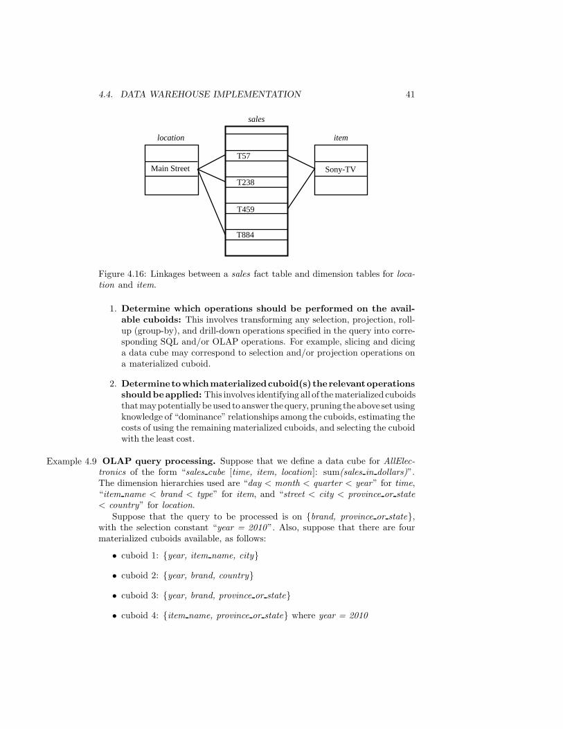
4.4. DATA WAREHOUSE IMPLEMENTATION 41
location
sales
item
Sony-TV
T57
T238
T459
Main Street
T884
Figure 4.16: Linkages between a sales fact table and dimension tables for loca-tion and item.
1. Determine which operations should be performed on the avail-able cuboids: This involves transforming any selection, projection, roll-up (group-by), and drill-down operations specified in the query into corre-sponding SQL and/or OLAP operations. For example, slicing and dicinga data cube may correspond to selection and/or projection operations ona materialized cuboid.
2. Determinetowhichmaterializedcuboid(s) therelevantoperationsshouldbeapplied: This involves identifying all of thematerialized cuboidsthatmaypotentially beused to answer thequery, pruning theabove setusingknowledge of “dominance” relationships among the cuboids, estimating thecosts of using the remaining materialized cuboids, and selecting the cuboidwith the least cost.
Example 4.9 OLAP query processing. Suppose that we define a data cube for AllElec-tronics of the form “sales cube [time, item, location]: sum(sales in dollars)”.The dimension hierarchies used are “day < month < quarter < year” for time,“item name < brand < type” for item, and “street < city < province or state< country” for location.
Suppose that the query to be processed is on {brand, province or state},with the selection constant “year = 2010”. Also, suppose that there are fourmaterialized cuboids available, as follows:
• cuboid 1: {year, item name, city}
• cuboid 2: {year, brand, country}
• cuboid 3: {year, brand, province or state}
• cuboid 4: {item name, province or state} where year = 2010
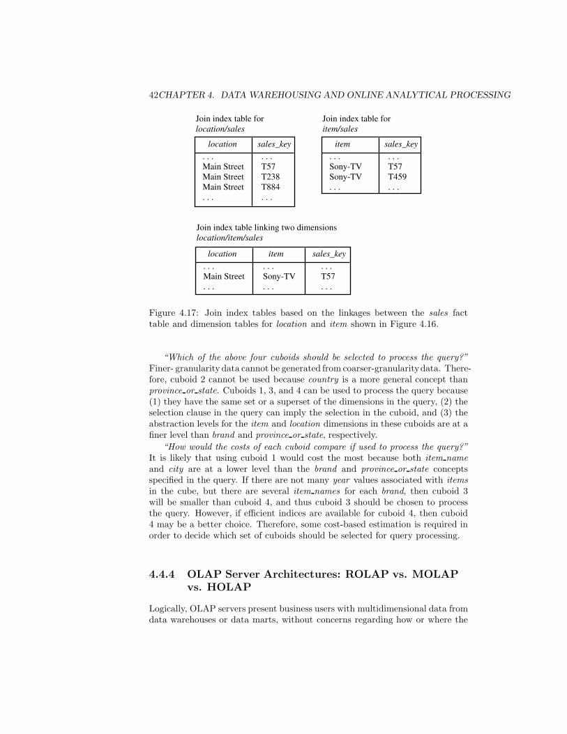
42CHAPTER 4. DATA WAREHOUSING AND ONLINE ANALYTICAL PROCESSING
Figure 4.17: Join index tables based on the linkages between the sales facttable and dimension tables for location and item shown in Figure 4.16.
“Which of the above four cuboids should be selected to process the query?”Finer- granularity data cannot be generated from coarser-granularitydata. There-fore, cuboid 2 cannot be used because country is a more general concept thanprovince or state. Cuboids 1, 3, and 4 can be used to process the query because(1) they have the same set or a superset of the dimensions in the query, (2) theselection clause in the query can imply the selection in the cuboid, and (3) theabstraction levels for the item and location dimensions in these cuboids are at afiner level than brand and province or state, respectively.
“How would the costs of each cuboid compare if used to process the query?”It is likely that using cuboid 1 would cost the most because both item nameand city are at a lower level than the brand and province or state conceptsspecified in the query. If there are not many year values associated with itemsin the cube, but there are several item names for each brand, then cuboid 3will be smaller than cuboid 4, and thus cuboid 3 should be chosen to processthe query. However, if efficient indices are available for cuboid 4, then cuboid4 may be a better choice. Therefore, some cost-based estimation is required inorder to decide which set of cuboids should be selected for query processing.
4.4.4 OLAP Server Architectures: ROLAP vs. MOLAP
vs. HOLAP
Logically, OLAP servers present business users with multidimensional data fromdata warehouses or data marts, without concerns regarding how or where the

4.4. DATA WAREHOUSE IMPLEMENTATION 43
data are stored. However, the physical architecture and implementation ofOLAP servers must consider data storage issues. Implementations of a ware-house server for OLAP processing include the following:
Relational OLAP (ROLAP) servers: These are the intermediate servers thatstand in between a relational back-end server and client front-end tools.They use a relational or extended-relational DBMS to store and managewarehouse data, and OLAP middleware to support missing pieces. ROLAPservers include optimization for each DBMS back end, implementation ofaggregation navigation logic, and additional tools and services. ROLAPtechnology tends to have greater scalability than MOLAP technology. TheDSS server of Microstrategy, for example, adopts the ROLAP approach.
MultidimensionalOLAP (MOLAP) servers: These servers support multi-dimensional views of data through array-based multidimensional storage en-gines. They map multidimensional views directly to data cube array struc-tures. Theadvantageofusingadata cube is that itallows fast indexing topre-computed summarizeddata. Notice thatwith multidimensional data stores,thestorageutilizationmaybe lowif thedataset is sparse. Insuchcases, sparsematrix compression techniques should be explored (Chapter 5).
Many MOLAP servers adopt a two-level storage representation to handledense and sparse data sets: denser subcubes are identified and stored as ar-ray structures, whereas sparse subcubes employ compression technology forefficient storage utilization.
Hybrid OLAP (HOLAP) servers: The hybrid OLAP approach combinesROLAP and MOLAP technology, benefiting from the greater scalability ofROLAP and the faster computation of MOLAP. For example, a HOLAPserver may allow large volumes of detail data to be stored in a relationaldatabase, while aggregations are kept in a separate MOLAP store. TheMicrosoft SQL Server 2000 supports a hybrid OLAP server.
Specialized SQL servers: To meet the growing demand of OLAP processingin relational databases, some database system vendors implement special-ized SQL servers that provide advanced query language and query pro-cessing support for SQL queries over star and snowflake schemas in aread-only environment.
Table 4.4: Single table for base and summary facts.RID item . . . day month quarter year dollars sold
1001 TV . . . 15 10 Q4 2010 250.601002 TV . . . 23 10 Q4 2010 175.00. . . . . . . . . . . . . . . . . . . . . . . .5001 TV . . . all 10 Q4 2010 45,786.08. . . . . . . . . . . . . . . . . . . . . . . .

44CHAPTER 4. DATA WAREHOUSING AND ONLINE ANALYTICAL PROCESSING
“How are data actually stored in ROLAP and MOLAP architectures?” Let’sfirst look at ROLAP. As its name implies, ROLAP uses relational tables to storedata for online analytical processing. Recall that the fact table associated witha base cuboid is referred to as a base fact table. The base fact table storesdata at the abstraction level indicated by the join keys in the schema for thegiven data cube. Aggregated data can also be stored in fact tables, referredto as summary fact tables. Some summary fact tables store both base facttable data and aggregated data, as in Example 3.10. Alternatively, separatesummary fact tables can be used for each level of abstraction, to store onlyaggregated data.
Example 4.10 A ROLAP data store. Table 4.4 shows a summary fact table that con-tains both base fact data and aggregated data. The schema of the table is“〈record identifier (RID), item, . . . , day, month, quarter, year, dollars sold〉”,where day, month, quarter, and year define the date of sales, and dollars soldis the sales amount. Consider the tuples with an RID of 1001 and 1002, re-spectively. The data of these tuples are at the base fact level, where the dateof sales is October 15, 2010, and October 23, 2010, respectively. Consider thetuple with an RID of 5001. This tuple is at a more general level of abstractionthan the tuples 1001 and 1002. The day value has been generalized to all, sothat the corresponding time value is October 2010. That is, the dollars soldamount shown is an aggregation representing the entire month of October 2010,rather than just October 15 or 23, 2010. The special value all is used to repre-sent subtotals in summarized data.
MOLAP uses multidimensional array structures to store data for onlineanalytical processing. This structure is discussed in the following section ondata warehouse implementation and, in greater detail, in Chapter 5.
Most data warehouse systems adopt a client-server architecture. A rela-tional data store always resides at the data warehouse/data mart server site.A multidimensional data store can reside at either the database server site orthe client site.
4.5 DataGeneralization byAttribute-Oriented In-
duction
Conceptually, data cube can be viewed as one kind of multidimensional datageneralization. In general, data generalization summarizes data by replacingrelatively low-level values (such as numeric values for an attribute age) withhigher-level concepts (such as young, middle-aged, and senior) or by reduc-ing the number of dimensions to summarize data in concept space involvingless number of dimensions (such as removing birth-date and telephone num-bers when summarizing the behavior of a group of students). Given the largeamount of data stored in databases, it is useful to be able to describe con-cepts in concise and succinct terms at generalized (rather than low) levels ofabstraction. Allowing data sets to be generalized at multiple levels of abstrac-
4.5. DATA GENERALIZATION BY ATTRIBUTE-ORIENTED INDUCTION45
tion facilitates users in examining the general behavior of the data. Given theAllElectronics database, for example, instead of examining individual customertransactions, sales managers may prefer to view the data generalized to higherlevels, such as summarized by customer groups according to geographic regions,frequency of purchases per group, and customer income.
This leads us to the notion of concept description, which is a form of datageneralization. A concept typically refers to a collection of data such as fre-quent buyers, graduate students, and so on. As a data mining task, conceptdescription is not a simple enumeration of the data. Instead, concept de-scription generates descriptions for the characterization and comparison ofthe data. It is sometimes called class description, when the concept to bedescribed refers to a class of objects. Characterization provides a concise andsuccinct summarization of the given collection of data, while concept or classcomparison (also known as discrimination) provides descriptions comparingtwo or more collections of data.
Up to this point, we have studied data cube (or OLAP) approaches toconcept description using multidimensional, multilevel data generalization indata warehouses. “Is data cube technology sufficient to accomplish all kinds ofconcept description tasks for large data sets?” Consider the following cases.
• Complex data types and aggregation: Data warehouses and OLAPtools are based on a multidimensional data model that views data inthe form of a data cube, consisting of dimensions (or attributes) andmeasures (aggregate functions). However, many current OLAP systemsconfine dimensions to nonnumeric data and measures to numeric data. Inreality, the database can include attributes of various data types, includ-ing numeric, nonnumeric, spatial, text, or image, which ideally should beincluded in the concept description. Furthermore, the aggregation of at-tributes in a database may include sophisticated data types, such as thecollection of nonnumeric data, the merging of spatial regions, the com-position of images, the integration of texts, and the grouping of objectpointers. Therefore, OLAP, with its restrictions on the possible dimen-sion and measure types, represents a simplified model for data analysis.Concept description should handle complex data types of the attributesand their aggregations, as necessary.
• User-control versus automation: Online analytical processing in datawarehouses is a user-controlled process. The selection of dimensions andthe application of OLAP operations, such as drill-down, roll-up, slicing,and dicing, are primarily directed and controlled by the users. Althoughthe control in most OLAP systems is quite user-friendly, users do require agood understanding of the role of each dimension. Furthermore, in order tofind a satisfactory description of the data, users may need to specify a longsequence ofOLAPoperations. It is oftendesirable to have amore automatedprocess that helps users determine which dimensions (or attributes) shouldbe included in the analysis, and the degree to which the given data set shouldbe generalized in order to produce an interesting summarization of the data.

46CHAPTER 4. DATA WAREHOUSING AND ONLINE ANALYTICAL PROCESSING
This section presents an alternative method for concept description, calledattribute-oriented induction, which works for complex types of data and relieson a data-driven generalization process.
4.5.1 Attribute-Oriented Induction for Data Characteriza-
tion
The attribute-oriented induction (AOI) approach to concept descriptionwas first proposed in 1989, a few years before the introduction of the data cube ap-proach. The data cube approach is essentially based on materialized views of thedata, which typically have been precomputed in a data warehouse. In general, itperforms off-line aggregation before an OLAP or data mining query is submittedfor processing. On the other hand, the attribute-oriented induction approach isbasically a query-oriented, generalization-based, online data analysis technique.Note that there is no inherent barrier distinguishing the two approaches based ononline aggregation versus off-line precomputation. Some aggregations in the datacube can be computed online, while off-line precomputation of multidimensionalspace can speed up attribute-oriented induction as well.
The general idea of attribute-oriented induction is to first collect the task-relevant data using a database query and then perform generalization based onthe examination of the number of distinct values of each attribute in the rel-evant set of data. The generalization is performed by either attribute removalor attribute generalization. Aggregation is performed by merging identical gen-eralized tuples and accumulating their respective counts. This reduces the sizeof the generalized data set. The resulting generalized relation can be mappedinto different forms for presentation to the user, such as charts or rules.
The following examples illustrate the process of attribute-oriented induction.We first discuss its use for characterization. The method is extended for themining of class comparisons in Section 4.5.3.
Example 4.11 A data mining query for characterization. Suppose that a user would liketo describe the general characteristics of graduate students in the Big Universitydatabase, given the attributes name, gender, major, birth place, birth date,residence, phone# (telephone number), and gpa (grade point average). A datamining query for this characterization can be expressed in the data miningquery language, DMQL, as follows:
use Big University DBmine characteristics as “Science Students”in relevance to name, gender, major, birth place, birth date, residence,
phone#, gpafrom studentwhere status in “graduate”
We will see how this example of a typical data mining query can applyattribute-oriented induction for mining characteristic descriptions.

4.5. DATA GENERALIZATION BY ATTRIBUTE-ORIENTED INDUCTION47
First, data focusing should be performed before attribute-oriented induc-tion. This step corresponds to the specification of the task-relevant data (i.e.,data for analysis). The data are collected based on the information providedin the data mining query. Because a data mining query is usually relevant toonly a portion of the database, selecting the relevant set of data not only makesmining more efficient, but also derives more meaningful results than mining theentire database.
Specifying the set of relevant attributes (i.e., attributes for mining, as indi-cated in DMQL with the in relevance to clause) may be difficult for the user.A user may select only a few attributes that he or she feels may be important,while missing others that could also play a role in the description. For exam-ple, suppose that the dimension birth place is defined by the attributes city,province or state, and country. Of these attributes, let’s say that the user hasonly thought to specify city. In order to allow generalization on the birth placedimension, the other attributes defining this dimension should also be included.In other words, having the system automatically include province or state andcountry as relevant attributes allows city to be generalized to these higher con-ceptual levels during the induction process.
At the other extreme, suppose that the user may have introduced too manyattributes by specifying all of the possible attributes with the clause “in rel-evance to ∗”. In this case, all of the attributes in the relation specified bythe from clause would be included in the analysis. Many of these attributesare unlikely to contribute to an interesting description. A correlation-based(Section 3.3.2) or entropy-based (Section 3.5.6) analysis method can be usedto perform attribute relevance analysis and filter out statistically irrelevantor weakly relevant attributes from the descriptive mining process. Other ap-proaches, such as attribute subset selection, are also described in Chapter 3.
“What does the ‘where status in “graduate”’ clause mean?” This whereclause implies that a concept hierarchy exists for the attribute status. Sucha concept hierarchy organizes primitive-level data values for status, such as“M.Sc.”, “M.A.”, “M.B.A.”, “Ph.D.”, “B.Sc.”, “B.A.”, into higher conceptuallevels, such as “graduate” and “undergraduate.” This use of concept hierarchiesdoes not appear in traditional relational query languages, yet is likely to becomea common feature in data mining query languages.
The data mining query presented above is transformed into the followingrelational query for the collection of the task-relevant set of data:
use Big University DBselect name, gender, major, birth place, birth date, residence, phone#, gpafrom studentwhere status in {“M.Sc.”, “M.A.”, “M.B.A.”, “Ph.D.”}
The transformed query is executed against the relational database, Big University DB,and returns the data shown in Table 4.5. This table is called the (task-relevant)initial working relation. It is the data on which induction will be performed.Note that each tuple is, in fact, a conjunction of attribute-value pairs. Hence,

48CHAPTER 4. DATA WAREHOUSING AND ONLINE ANALYTICAL PROCESSING
Table 4.5: Initial working relation: a collection of task-relevant data.name gender major birth place birth date residence phone# gpa
Jim Woodman M CS Vancouver, BC, Canada 8-12-76 3511 Main St., Richmond 687-4598 3.67Scott Lachance M CS Montreal, Que, Canada 28-7-75 345 1st Ave., Richmond 253-9106 3.70Laura Lee F physics Seattle, WA, USA 25-8-70 125 Austin Ave., Burnaby 420-5232 3.83· · · · · · · · · · · · · · · · · · · · · · · ·
we can think of a tuple within a relation as a rule of conjuncts, and of inductionon the relation as the generalization of these rules.
“Now that the data are ready for attribute-oriented induction, how is attribute-oriented induction performed?” The essential operation of attribute-orientedinduction is data generalization, which can be performed in either of two wayson the initial working relation: attribute removal and attribute generalization.
Attribute removal is based on the following rule: If there is a large set ofdistinct values for an attribute of the initial working relation, but either (1) thereis no generalization operator on the attribute (e.g., there is no concept hierar-chy defined for the attribute), or (2) its higher-level concepts are expressed interms of other attributes, then the attribute should be removed from the workingrelation.
Let’s examine the reasoning behind this rule. An attribute-value pair rep-resents a conjunct in a generalized tuple, or rule. The removal of a conjuncteliminates a constraint and thus generalizes the rule. If, as in case 1, thereis a large set of distinct values for an attribute but there is no generalizationoperator for it, the attribute should be removed because it cannot be gen-eralized, and preserving it would imply keeping a large number of disjuncts,which contradicts the goal of generating concise rules. On the other hand, con-sider case 2, where the higher-level concepts of the attribute are expressed interms of other attributes. For example, suppose that the attribute in questionis street, whose higher-level concepts are represented by the attributes 〈city,province or state, country〉. The removal of street is equivalent to the applica-tion of a generalization operator. This rule corresponds to the generalizationrule known as dropping conditions in the machine learning literature on learningfrom examples .
Attribute generalization is based on the following rule: If there is a largeset of distinct values for an attribute in the initial working relation, and thereexists a set of generalization operators on the attribute, then a generalizationoperator should be selected and applied to the attribute. This rule is based on thefollowing reasoning. Use of a generalization operator to generalize an attributevalue within a tuple, or rule, in the working relation will make the rule covermore of the original data tuples, thus generalizing the concept it represents.This corresponds to the generalization rule known as climbing generalizationtrees in learning from examples, or concept tree ascension.
Both rules, attribute removal and attribute generalization, claim that if there

4.5. DATA GENERALIZATION BY ATTRIBUTE-ORIENTED INDUCTION49
is a large set of distinct values for an attribute, further generalization shouldbe applied. This raises the question: how large is “a large set of distinct valuesfor an attribute” considered to be?
Depending on the attributes or application involved, a user may prefer someattributes to remain at a rather low abstraction level while others are generalizedto higher levels. The control of how high an attribute should be generalized istypically quite subjective. The control of this process is called attribute gen-eralization control. If the attribute is generalized “too high,” it may lead toovergeneralization, and the resulting rules may not be very informative. On theother hand, if the attribute is not generalized to a “sufficiently high level,” thenundergeneralization may result, where the rules obtained may not be informativeeither. Thus, a balance should be attained in attribute-oriented generalization.
There are many possible ways to control a generalization process. We willdescribe two common approaches and then illustrate how they work with anexample.
The first technique, called attribute generalization threshold control,either sets one generalization threshold for all of the attributes, or sets onethreshold for each attribute. If the number of distinct values in an attributeis greater than the attribute threshold, further attribute removal or attributegeneralization should be performed. Data mining systems typically have adefault attribute threshold value generally ranging from 2 to 8 and should allowexperts and users to modify the threshold values as well. If a user feels that thegeneralization reaches too high a level for a particular attribute, the thresholdcan be increased. This corresponds to drilling down along the attribute. Also,to further generalize a relation, the user can reduce the threshold of a particularattribute, which corresponds to rolling up along the attribute.
The second technique, called generalized relation threshold control,sets a threshold for the generalized relation. If the number of (distinct) tuplesin the generalized relation is greater than the threshold, further generalizationshould be performed. Otherwise, no further generalization should be performed.Such a threshold may also be preset in the data mining system (usually withina range of 10 to 30), or set by an expert or user, and should be adjustable.For example, if a user feels that the generalized relation is too small, he or shecan increase the threshold, which implies drilling down. Otherwise, to furthergeneralize a relation, the threshold can be reduced, which implies rolling up.
These two techniques can be applied in sequence: first apply the attributethreshold control technique to generalize each attribute, and then apply relationthreshold control to further reduce the size of the generalized relation. Nomatter which generalization control technique is applied, the user should beallowed to adjust the generalization thresholds in order to obtain interestingconcept descriptions.
In many database-oriented induction processes, users are interested in ob-taining quantitative or statistical information about the data at different levelsof abstraction. Thus, it is important to accumulate count and other aggregatevalues in the induction process. Conceptually, this is performed as follows. Theaggregate function, count, is associated with each database tuple. Its value for

50CHAPTER4. DATAWAREHOUSINGANDONLINEANALYTICALPROCESSING
each tuple in the initial working relation is initialized to 1. Through attributeremoval and attribute generalization, tuples within the initial working relationmay be generalized, resulting in groups of identical tuples. In this case, allof the identical tuples forming a group should be merged into one tuple. Thecount of this new, generalized tuple is set to the total number of tuples from theinitial working relation that are represented by (i.e., were merged into) the newgeneralized tuple. For example, suppose that by attribute-oriented induction,52 data tuples from the initial working relation are all generalized to the sametuple, T . That is, the generalization of these 52 tuples resulted in 52 identicalinstances of tuple T . These 52 identical tuples are merged to form one instanceof T , whose count is set to 52. Other popular aggregate functions that couldalso be associated with each tuple include sum and avg. For a given generalizedtuple, sum contains the sum of the values of a given numeric attribute for theinitial working relation tuples making up the generalized tuple. Suppose thattuple T contained sum(units sold) as an aggregate function. The sum value fortuple T would then be set to the total number of units sold for each of the 52tuples. The aggregate avg (average) is computed according to the formula, avg= sum/count.
Example 4.12 Attribute-oriented induction. Here we show how attribute-oriented induc-tion is performed on the initial working relation of Table 4.5. For each attributeof the relation, the generalization proceeds as follows:
1. name: Since there are a large number of distinct values for name andthere is no generalization operation defined on it, this attribute is re-moved.
2. gender: Since there are only two distinct values for gender, this attributeis retained and no generalization is performed on it.
3. major: Suppose that a concept hierarchy has been defined that allows theattribute major to be generalized to the values {arts&science, engineer-ing, business}. Suppose also that the attribute generalization threshold isset to 5, and that there are more than 20 distinct values for major in theinitial working relation. By attribute generalization and attribute gen-eralization control, major is therefore generalized by climbing the givenconcept hierarchy.
4. birth place: This attribute has a large number of distinct values; therefore,we would like to generalize it. Suppose that a concept hierarchy exists forbirth place, defined as “city < province or state < country”. If the numberof distinct values for country in the initial working relation is greaterthan the attribute generalization threshold, then birth place should beremoved, because even though a generalization operator exists for it, thegeneralization threshold would not be satisfied. If instead, the numberof distinct values for country is less than the attribute generalizationthreshold, then birth place should be generalized to birth country.

4.5. DATA GENERALIZATION BY ATTRIBUTE-ORIENTED INDUCTION51
5. birth date: Suppose that a hierarchy exists that can generalize birth date toage, and age to age range, and that the number of age ranges (or intervals) issmall with respect to the attribute generalization threshold. Generalizationof birth date should therefore take place.
6. residence: Suppose that residence is definedby theattributesnumber, street,residence city,residence province or state,andresidence country. Thenum-ber ofdistinctvalues fornumber and street will likelybeveryhigh, since theseconcepts are quite low level. The attributes number and street should there-forebe removed, so that residence is thengeneralized to residence city, whichcontains fewer distinct values.
7. phone#: As with the attribute name above, this attribute contains toomany distinct values and should therefore be removed in generalization.
8. gpa: Suppose that a concept hierarchy exists for gpa that groups values forgrade point average into numerical intervals like {3.75–4.0, 3.5–3.75,. . . },which in turn are grouped into descriptive values, such as {excellent, verygood,. . . }. The attribute can therefore be generalized.
The generalization process will result in groups of identical tuples. Forexample, the first two tuples of Table 4.5 both generalize to the same identicaltuple (namely, the first tuple shown in Table 4.6). Such identical tuples arethen merged into one, with their counts accumulated. This process leads to thegeneralized relation shown in Table 4.6.
Based on the vocabulary used in OLAP, we may view count as a measure,and the remaining attributes as dimensions. Note that aggregate functions,such as sum, may be applied to numerical attributes, like salary and sales.These attributes are referred to as measure attributes.
4.5.2 Efficient Implementation of Attribute-Oriented In-
duction
“How is attribute-oriented induction actually implemented?” The previous sub-section provided an introduction to attribute-oriented induction. The generalprocedure is summarized in Figure 4.18. The efficiency of this algorithm isanalyzed as follows:
• Step 1 of the algorithm is essentially a relational query to collect the task-relevant data into the working relation, W . Its processing efficiency
Table 4.6: A generalized relation obtained by attribute-oriented induction on thedata of Table 4.5.gender major birth country age range residence city gpa count
M Science Canada 20 – 25 Richmond very good 16F Science Foreign 25 – 30 Burnaby excellent 22· · · · · · · · · · · · · · · · · · · · ·

52CHAPTER 4. DATA WAREHOUSING AND ONLINE ANALYTICAL PROCESSING
Algorithm: Attribute oriented induction. Mining generalized characteristics in a relational database givena user’s data mining request.
Input:
• DB, a relational database;
• DMQuery, a data mining query;
• a list, a list of attributes (containing attributes, ai);
• Gen(ai), a set of concept hierarchies or generalization operators on attributes, ai;
• a gen thresh(ai), attribute generalization thresholds for each ai.
Output: P , a Prime generalized relation.
Method:
1. W ← get task relevant data (DMQuery, DB); // Let W , the working relation, hold the task-relevantdata.
2. prepare for generalization (W ); // This is implemented as follows.
(a) Scan W and collect the distinct values for each attribute, ai. (Note: If W is very large,this may be done by examining a sample of W .)
(b) For each attribute ai, determine whether ai should be removed, and if not, computeits minimum desired level Li based on its given or default attribute threshold, and
determine the mapping-pairs (v, v′), where v is a distinct value of ai in W , and v′ isits corresponding generalized value at level Li.
3. P ← generalization (W ),
The Prime generalized relation, P , is derived by replacing each value v in W by its correspondingv′ in the mapping while accumulating count and computing any other aggregate values.
This step can be implemented efficiently using either of the two following variations:
(a) For each generalized tuple, insert the tuple into a sorted prime relation P by a binarysearch: if the tuple is already in P , simply increase its count and other aggregate valuesaccordingly; otherwise, insert it into P .
(b) Since in most cases the number of distinct values at the prime relation level is small,the prime relation can be coded as an m-dimensional array where m is the numberof attributes in P , and each dimension contains the corresponding generalized attributevalues. Each array element holds the corresponding count and other aggregation values,if any. The insertion of a generalized tuple is performed by measure aggregation in thecorresponding array element.
Figure 4.18: Basic algorithm for attribute-oriented induction.
depends on the query processing methods used. Given the successfulimplementation and commercialization of database systems, this step isexpected to have good performance.
• Step 2 collects statistics on the working relation. This requires scanningthe relation at most once. The cost for computing the minimum desiredlevel and determining the mapping pairs, (v, v′), for each attribute isdependent on the number of distinct values for each attribute and issmaller than |W |, the number of tuples in the working relation. Noticeit may not be necessary to scan the working relation once since if theworking relation is large, a sample of such a relation will be sufficient toget statistics and determine which attributes to be generalized to certainhigh-level and which attributes to be removed. Moreover, such statisticsmay also be obtained in the process of extracting and generating workingrelation in Step 1.
• Step 3 derives the prime relation, P . This is performed by scan eachtuple in the working relation and inserting generalized tuples into P .There are a total of |W | tuples in W and p tuples in P . For each tuple,

4.5. DATA GENERALIZATION BY ATTRIBUTE-ORIENTED INDUCTION53
Table 4.7: A generalized relation for the sales last year.location item sales (in million dollars) count (in thousands)
Asia TV 15 300Europe TV 12 250North America TV 28 450Asia computer 120 1000Europe computer 150 1200North America computer 200 1800
t, in W , we substitute its attribute values based on the derived mapping-pairs. This results in a generalized tuple, t′. If variation (a) is adopted,each t′ takes O(log p) to find the location for count increment or tupleinsertion. Thus the total time complexity is O(|W | × log p) for all of thegeneralized tuples. If variation (b) is adopted, each t′ takes O(1) to findthe tuple for count increment. Thus the overall time complexity is O(N)for all of the generalized tuples.
Many data analysis tasks need to examine a good number of dimensions orattributes. This may involve dynamically introducing and testing additionalattributes rather than just those specified in the mining query. Moreover, auser with little knowledge of the truly relevant set of data may simply specify“in relevance to ∗” in the mining query, which includes all of the attributes intothe analysis. Therefore, an advanced concept description mining process needsto perform attribute relevance analysis on large sets of attributes to select themost relevant ones. Such analysis may employ correlation or entropy measures,as described in Chapter 3 on data preprocessing.
Example 4.13 Presentation of generalization results. Suppose that attribute-orientedinduction was performed on a sales relation of the AllElectronics database,resulting in the generalized description of Table 4.7 for sales last year. Thedescription is shown in the form of a generalized relation. Table 4.6 of Exam-ple 4.11 is another example of a generalized relation.
Such generalized relations can also be presented in the form of cross tabu-lation forms, various kinds of graphic presentation (such as pie charts and barcharts), and quantitative characteristics rules (i.e., showing how different valuecombinations are distributed in the generalized relation).
4.5.3 Attribute-Oriented Induction for Class Comparisons
In many applications, users may not be interested in having a single class(or concept) described or characterized, but rather would prefer to mine adescription that compares or distinguishes one class (or concept) from othercomparable classes (or concepts). Class discrimination or comparison (here-after referred to as class comparison) mines descriptions that distinguish a

54CHAPTER 4. DATA WAREHOUSING AND ONLINE ANALYTICAL PROCESSING
target class from its contrasting classes. Notice that the target and contrastingclasses must be comparable in the sense that they share similar dimensions andattributes. For example, the three classes, person, address, and item, are notcomparable. However, the sales in the last three years are comparable classes,and so are computer science students versus physics students.
Our discussions on class characterization in the previous sections handlemultilevel data summarization and characterization in a single class. The tech-niques developed can be extended to handle class comparison across severalcomparable classes. For example, the attribute generalization process describedfor class characterization can be modified so that the generalization is per-formed synchronously among all the classes compared. This allows the at-tributes in all of the classes to be generalized to the same levels of abstraction.Suppose, for instance, that we are given the AllElectronics data for sales in 2009and sales in 2010 and would like to compare these two classes. Consider thedimension location with abstractions at the city, province or state, and coun-try levels. Data in each class should be generalized to the same location level.That is, they are all synchronously generalized to either the city level, or theprovince or state level, or the country level. Ideally, this is more useful thancomparing, say, the sales in Vancouver in 2009 with the sales in the UnitedStates in 2010 (i.e., where each set of sales data is generalized to a differentlevel). The users, however, should have the option to overwrite such an auto-mated, synchronous comparison with their own choices, when preferred.
“How is class comparison performed?” In general, the procedure is as fol-lows:
1. Data collection: The set of relevant data in the database is collectedby query processing and is partitioned respectively into a target class andone or a set of contrasting classes.
2. Dimension relevance analysis: If there are many dimensions, then di-mension relevance analysis should be performed on these classes to selectonly the highly relevant dimensions for further analysis. Correlation orentropy-based measures can be used for this step (Chapter 3).
3. Synchronous generalization: Generalization is performed on the tar-get class to the level controlled by a user- or expert-specified dimensionthreshold, which results in a prime target class relation. The conceptsin the contrasting class(es) are generalized to the same level as those inthe prime target class relation, forming the prime contrasting class(es)relation.
4. Presentation of the derived comparison: The resulting class com-parison description can be visualized in the form of tables, graphs, andrules. This presentation usually includes a “contrasting” measure suchas count% (percentage count) that reflects the comparison between thetarget and contrasting classes. The user can adjust the comparison de-scription by applying drill-down, roll-up, and other OLAP operations tothe target and contrasting classes, as desired.

4.5. DATA GENERALIZATION BY ATTRIBUTE-ORIENTED INDUCTION55
The above discussion outlines a general algorithm for mining comparisons indatabases. In comparison with characterization, the above algorithm involvessynchronous generalization of the target class with the contrasting classes, sothat classes are simultaneously compared at the same levels of abstraction.
The following example mines a class comparison describing the graduatestudents and the undergraduate students at Big University.
Example 4.14 Mining a class comparison. Suppose that you would like to compare thegeneral properties between the graduate students and the undergraduate stu-dents at Big University, given the attributes name, gender, major, birth place,birth date, residence, phone#, and gpa.
This data mining task can be expressed in DMQL as follows:
use Big University DBmine comparison as “grad vs undergrad students”in relevance to name, gender, major, birth place, birth date, residence,
phone#, gpafor “graduate students”where status in “graduate”versus “undergraduate students”where status in “undergraduate”analyze count%from student
Let’s see how this typical example of a data mining query for mining com-parison descriptions can be processed.
First, the query is transformed into two relational queries that collect twosets of task-relevant data: one for the initial target class working relation, andthe other for the initial contrasting class working relation, as shown in Tables 4.8and 4.9. This can also be viewed as the construction of a data cube, wherethe status {graduate, undergraduate} serves as one dimension, and the otherattributes form the remaining dimensions.
Second, dimension relevance analysis can be performed, when necessary, onthe two classes of data. After this analysis, irrelevant or weakly relevant dimen-sions, such as name, gender, birth place, residence, and phone#, are removedfrom the resulting classes. Only the highly relevant attributes are included inthe subsequent analysis.
Table 4.8: Initial working relations: the target class (graduate students)name gender major birth place birth date residence phone# gpa
Jim Woodman M CS Vancouver, BC, Canada 8-12-76 3511 Main St., Richmond 687-4598 3.67Scott Lachance M CS Montreal, Que, Canada 28-7-75 345 1st Ave., Vancouver 253-9106 3.70Laura Lee F Physics Seattle, WA, USA 25-8-70 125 Austin Ave., Burnaby 420-5232 3.83· · · · · · · · · · · · · · · · · · · · · · · ·

56CHAPTER 4. DATA WAREHOUSING AND ONLINE ANALYTICAL PROCESSING
Table 4.9: Initial working relations: the contrasting class (undergraduate students)name gender major birth place birth date residence phone# gpa
Bob Schumann M Chemistry Calgary, Alt, Canada 10-1-78 2642 Halifax St., Burnaby 294-4291 2.96Amy Eau F Biology Golden, BC, Canada 30-3-76 463 Sunset Cres., Vancouver 681-5417 3.52
· · · · · · · · · · · · · · · · · · · · · · · ·
Table 4.10: Prime generalized relation for the targetclass (graduate students)major age range gpa count%
Science 21...25 good 5.53%Science 26...30 good 5.02%Science over 30 very good 5.86%
· · · · · · · · · · · ·
Business over 30 excellent 4.68%
Third, synchronous generalization is performed: Generalization is performedon the target class to the levels controlled by user- or expert-specified dimensionthresholds, forming the prime target class relation. The contrasting class isgeneralized to the same levels as those in the prime target class relation, formingthe prime contrasting class(es) relation, as presented in Tables 4.10 and 4.11.In comparison with undergraduate students, graduate students tend to be olderand have a higher GPA, in general.
Finally, the resulting class comparison is presented in the form of tables,graphs, and/or rules. This visualization includes a contrasting measure (suchas count%) that compares between the target class and the contrasting class.For example, 5.02% of the graduate students majoring in Science are between 26and 30 years of age and have a “good” GPA, while only 2.32% of undergraduateshave these same characteristics. Drilling and other OLAP operations may beperformed on the target and contrasting classes as deemed necessary by theuser in order to adjust the abstraction levels of the final description.
As shown in the above introduction to attribute-oriented induction for datacharacterization and generalization, attribute-oriented induction provides an
Table 4.11: Prime generalized relation for thecontrasting class (undergraduate students)major age range gpa count%
Science 16...20 fair 5.53%Science 16...20 good 4.53%
· · · · · · · · · · · ·
Science 26...30 good 2.32%· · · · · · · · · · · ·
Business over 30 excellent 0.68%

4.6. SUMMARY 57
alternative data generalization method in comparison with data cube approach.It is not confined to relational data since such induction can be performed onspatial, multimedia, sequence and other kinds of data sets, and there is no needto precompute a data cube since generalization can be performed online uponreceiving a user’s query. Moreover, automated analysis can be added to suchan induction process to automatically filter out some irrelevant or unimportantattributes and add some closed relevant ones. Analysis can also be performedto generalize the data to certain high level for further analysis. However, sinceattribute-oriented induction automatically generalize data to certain high-level,it cannot efficiently support the process of drilling down to the level deeper thanthose provided in the generalized relation. It is desirable to integrate data cubetechnology with attribute-oriented induction to balance precomputation andonline computation and to support fast online computation when it is necessaryto drill down to the level deeper than that provided in the generalized relation.
4.6 Summary
• A data warehouse is a subject-oriented, integrated, time-variant, andnonvolatile collection of data organized in support of management deci-sion making. Several factors distinguish data warehouses from operationaldatabases. Because the two systems provide quite different functionali-ties and require different kinds of data, it is necessary to maintain datawarehouses separately from operational databases.
• Data warehouses often adopt a three-tier architecture. The bottom tieris a warehouse database server, which is typically a relational database sys-tem. The middle tier is an OLAP server, and the top tier is a client, contain-ing query and reporting tools.
• A data warehouse contains back-end tools and utilities for populatingand refreshing the warehouse. These cover data extraction, data cleaning,data transformation, loading, refreshing, and warehouse management.
• Data warehouse metadata are data defining the warehouse objects. Ametadata repository provides details regarding the warehouse structure,data history, the algorithms used for summarization, mappings from thesource data to warehouse form, system performance, and business termsand issues.
• A multidimensional data model is typically used for the design of cor-porate data warehouses and departmental data marts. Such a model canadopt a star schema, snowflake schema, or fact constellation schema. Thecore of the multidimensional model is the data cube, which consists of alarge set of facts (or measures) and a number of dimensions. Dimensionsare the entities or perspectives with respect to which an organizationwants to keep records and are hierarchical in nature.

58CHAPTER 4. DATA WAREHOUSING AND ONLINE ANALYTICAL PROCESSING
• A data cube consists of a lattice of cuboids, each corresponding to adifferent degree of summarization of the given multidimensional data.
• Concept hierarchies organize the values of attributes or dimensionsinto gradual levels of abstraction. They are useful in mining at multiplelevels of abstraction.
• Online analytical processing (OLAP) can be performed in data ware-houses/marts using the multidimensional data model. Typical OLAP op-erations include roll-up, drill-(down, across, through), slice-and-dice, pivot(rotate), as well as statistical operations such as ranking and computingmoving averages and growth rates. OLAP operations can be implementedefficiently using the data cube structure.
• Data warehouses are used for information processing (querying and report-ing), analytical processing (which allows users to navigate through sum-marized and detailed data by OLAP operations), and data mining (whichsupports knowledge discovery). OLAP-based data mining is referred to asmultidimensional data mining (also known as exploratory multidimen-sional data mining, online analytical mining, or OLAM). It emphasizes theinteractive and exploratory nature of data mining.
• OLAP servers may adopt a relational OLAP (ROLAP), a multidi-mensional OLAP (MOLAP), or a hybrid OLAP (HOLAP) imple-mentation. A ROLAP server uses an extended relational DBMS thatmaps OLAP operations on multidimensional data to standard relationaloperations. A MOLAP server maps multidimensional data views directlyto array structures. A HOLAP server combines ROLAP and MOLAP.For example, it may use ROLAP for historical data while maintainingfrequently accessed data in a separate MOLAP store.
• Full materialization refers to the computation of all of the cuboids in thelattice defining a data cube. It typically requires an excessive amount of stor-age space, particularly as the number of dimensions and size of associatedconcept hierarchies grow. This problem is known as the curse of dimen-sionality. Alternatively, partial materialization is the selective compu-tation of a subset of the cuboids or subcubes in the lattice. For example, aniceberg cube is a data cube that stores only those cube cells whose aggre-gate value (e.g., count) is above some minimum support threshold.
• OLAP query processing can be made more efficient with the use of index-ing techniques. In bitmap indexing, each attribute has its own bitmapindex table. Bitmap indexing reduces join, aggregation, and comparisonoperations to bit arithmetic. Join indexing registers the joinable rowsof two or more relations from a relational database, reducing the overallcost of OLAP join operations. Bitmapped join indexing, which com-bines the bitmap and join index methods, can be used to further speedup OLAP query processing.

4.7. EXERCISES 59
• Data generalization is a process that abstracts a large set of task-relevant data in a database from a relatively low conceptual level to higherconceptual levels. Data generalization approaches include data cube–based data aggregation and attribute-oriented induction. item Conceptdescription is the most basic form of descriptive data mining. It de-scribes a given set of task-relevant data in a concise and summarativemanner, presenting interesting general properties of the data. Concept(or class) description consists of characterization and comparison (ordiscrimination). The former summarizes and describes a collection ofdata, called the target class, whereas the latter summarizes and dis-tinguishes one collection of data, called the target class, from othercollection(s) of data, collectively called the contrasting class(es).
• Concept characterization can be implemented using data cube (OLAP-based) approaches and the attribute-oriented induction approach.These are attribute- or dimension-based generalization approaches. Theattribute-oriented induction approach consists of the following tech-niques: data focusing, data generalization by attribute removal or attributegeneralization, count and aggregate value accumulation, attribute general-ization control, and generalization data visualization.
• Concept comparison can be performed using the attribute-oriented in-duction or data cube approaches in a manner similar to concept charac-terization. Generalized tuples from the target and contrasting classes canbe quantitatively compared and contrasted.
4.7 Exercises
1. State why, for the integration of multiple heterogeneous information sources,many companies in industry prefer the update-driven approach (whichconstructs and uses data warehouses), rather than the query-driven ap-proach (which applies wrappers and integrators). Describe situationswhere the query-driven approach is preferable over the update-driven ap-proach.
2. Briefly compare the following concepts. You may use an example to ex-plain your point(s).
(a) Snowflake schema, fact constellation, starnet query model
(b) Data cleaning, data transformation, refresh
(c) Discovery-driven cube, multifeature cube, virtual warehouse
3. Suppose that a data warehouse consists of the three dimensions time,doctor, and patient, and the two measures count and charge, where chargeis the fee that a doctor charges a patient for a visit.

60CHAPTER 4. DATA WAREHOUSING AND ONLINE ANALYTICAL PROCESSING
(a) Enumerate three classes of schemas that are popularly used for mod-eling data warehouses.
(b) Draw a schema diagram for the above data warehouse using one ofthe schema classes listed in (a).
(c) Starting with the base cuboid [day, doctor, patient], what specificOLAP operations should be performed in order to list the total feecollected by each doctor in 2004?
(d) To obtain the same list, write an SQL query assuming the data isstored in a relational database with the schema fee (day, month,year, doctor, hospital, patient, count, charge).
4. Suppose that a data warehouse for Big-University consists of the fol-lowing four dimensions: student, course, semester, and instructor, andtwo measures count and avg grade. When at the lowest conceptual level(e.g., for a given student, course, semester, and instructor combination),the avg grade measure stores the actual course grade of the student. Athigher conceptual levels, avg grade stores the average grade for the givencombination.
(a) Draw a snowflake schema diagram for the data warehouse.
(b) Starting with the base cuboid [student, course, semester, instructor],what specific OLAP operations (e.g., roll-up from semester to year)should one perform in order to list the average grade of CS coursesfor each Big-University student.
(c) If each dimension has five levels (including all), such as “student <
major < status < university < all”, how many cuboids will this cubecontain (including the base and apex cuboids)?
5. Suppose that a data warehouse consists of the four dimensions, date,spectator, location, and game, and the two measures, count and charge,where charge is the fare that a spectator pays when watching a game ona given date. Spectators may be students, adults, or seniors, with eachcategory having its own charge rate.
(a) Draw a star schema diagram for the data warehouse.
(b) Starting with the base cuboid [date, spectator, location, game], whatspecific OLAP operations should one perform in order to list thetotal charge paid by student spectators at GM Place in 2004?
(c) Bitmap indexing is useful in data warehousing. Taking this cubeas an example, briefly discuss advantages and problems of using abitmap index structure.
6. A data warehouse can be modeled by either a star schema or a snowflakeschema. Briefly describe the similarities and the differences of the two

4.7. EXERCISES 61
models, and then analyze their advantages and disadvantages with regardto one another. Give your opinion of which might be more empiricallyuseful and state the reasons behind your answer.
7. Design a data warehouse for a regional weather bureau. The weather bu-reau has about 1,000 probes, which are scattered throughout various landand ocean locations in the region to collect basic weather data, includ-ing air pressure, temperature, and precipitation at each hour. All dataare sent to the central station, which has collected such data for over 10years. Your design should facilitate efficient querying and on-line analyt-ical processing, and derive general weather patterns in multidimensionalspace.
8. A popular data warehouse implementation is to construct a multidimen-sional database, known as a data cube. Unfortunately, this may oftengenerate a huge, yet very sparse multidimensional matrix.
(a) Present an example illustrating such a huge and sparse data cube.
(b) Design an implementation method that can elegantly overcome thissparse matrix problem. Note that you need to explain your datastructures in detail and discuss the space needed, as well as how toretrieve data from your structures.
(c) Modify your design in (b) to handle incremental data updates. Givethe reasoning behind your new design.
9. Regarding the computation of measures in a data cube:
(a) Enumerate three categories of measures, based on the kind of aggre-gate functions used in computing a data cube.
(b) For a data cube with the three dimensions time, location, and item,which category does the function variance belong to? Describe howto compute it if the cube is partitioned into many chunks.
Hint: The formula for computing variance is 1
N
∑N
i=1(xi − x̄i)
2,where x̄i is the average of xis.
(c) Suppose the function is “top 10 sales.” Discuss how to efficientlycompute this measure in a data cube.
10. Suppose a company would like to design a data warehouse that may fa-cilitate the analysis of moving vehicles in an online analytical processingmanner. The company registers huge amounts of auto movement datain the format of (Auto ID, location, speed, time). Each Auto ID repre-sents one vehicle associated with information, such as vehicle category,driver category, etc., and each location could be associated with a streetin a city. You may assume a street map is available for the city.
(a) Design such a data warehouse that may facilitate effective on-lineanalytical processing in multidimensional space.

62CHAPTER 4. DATA WAREHOUSING AND ONLINE ANALYTICAL PROCESSING
(b) The movement data may contain noise. Discuss how you can developa method that may automatically discover some data records arelikely erroneously registered in the data repository.
(c) The movement data may be sparse. Discuss how you can developa method that may construct reliable data warehouse despite of thesparsity of data.
(d) If one wants to drive from A to B starting at a particular time,discuss how a system may use the data in this warehouse to workout a fast route for the driver.
11. RFID has been used substantially to trace object movements and performinventory control. An RFID reader can successfully read an RFID tag atcertain limited distance at any scheduled time. Suppose a company wouldlike to design a data warehouse that may facilitate the analysis of objectswith RFID tags in an online analytical processing manner. The companyregisters huge amounts of RFID data in the format of (RFID, at-location,time), and also has some information about the objects carrying the RFIDtag, e.g., (RFID, product-name, product-category, producer, produced-date, price).
(a) Design a data warehouse that may facilitate effective registrationand on-line analytical processing of such data.
(b) The RFID data may contain lots of redundant information. Discussone method that maximally reduces redundancy in the registrationof them in the RFID data warehouse.
(c) The RFID data may contain lots of noises, such as missing registra-tion, misreading of IDs. Discuss one method that clean-up the noisedata effectively in the RFID data warehouse.
(d) One may like to perform online analytical processing to find howmany TV sets shipping from the LA seaport to BestBuy in Cham-paign by month, by brand, and by price-range. Outline how this canbe done efficiently if you store such RFID data in the warehouse.
(e) If a customer brings back a jug of milk and complains it is rottenbefore its expiration data, discuss how you could investigate sucha case in the warehouse to find out what could be the problem, inshipping or in storage.
12. In many applications, new data sets are incrementally added to the ex-isting large data sets. Thus an important consideration is whether ameasure can be computed efficiently in incremental manner. Use count,standard deviation, and median as examples to show that a distributive oralgebraic measure facilitates efficient incremental computation, whereas aholistic measure does not.
13. Suppose that we need to record three measures in a data cube: min, aver-age, and median. Design an efficient computation and storage method for

4.7. EXERCISES 63
each measure given that the cube allows data to be deleted incrementally(i.e., in small portions at a time) from the cube.
14. In data warehouse technology, a multiple dimensional view can be imple-mented by a relational database technique (ROLAP), or by a multidimen-sional database technique (MOLAP), or by a hybrid database technique(HOLAP).
(a) Briefly describe each implementation technique.
(b) For each technique, explain how each of the following functions maybe implemented:
i. The generation of a data warehouse (including aggregation)
ii. Roll-up
iii. Drill-down
iv. Incremental updating
Which implementation techniques do you prefer, and why?
15. Suppose that a data warehouse contains 20 dimensions, each with aboutfive levels of granularity.
(a) Users are mainly interested in four particular dimensions, each hav-ing three frequently accessed levels for rolling up and drilling down.How would you design a data cube structure to support this prefer-ence efficiently?
(b) At times, a user may want to drill through the cube, down to the rawdata for one or two particular dimensions. How would you supportthis feature?
16. A data cube, C, has n dimensions, and each dimension has exactly p
distinct values in the base cuboid. Assume that there are no concepthierarchies associated with the dimensions.
(a) What is the maximum number of cells possible in the base cuboid?
(b) What is the minimum number of cells possible in the base cuboid?
(c) What is the maximum number of cells possible (including both basecells and aggregate cells) in the data cube, C?
(d) What is the minimum number of cells possible in the data cube, C?
17. What are the differences between the three main types of data warehouseusage: information processing, analytical processing, and data mining?Discuss the motivation behind OLAP mining (OLAM).

64CHAPTER 4. DATA WAREHOUSING AND ONLINE ANALYTICAL PROCESSING
4.8 Bibliographic Notes
There are a good number of introductory-level textbooks on data warehousingand OLAP technology, including Kimball and Ross [KR02], Imhoff, Galemmoand Geiger [IGG03], Inmon [Inm96], Berson and Smith [BS97], and Thom-sen [Tho97]. Chaudhuri and Dayal [CD97] provide a general overview of datawarehousing and OLAP technology. A set of research papers on material-ized views and data warehouse implementations were collected in MaterializedViews: Techniques, Implementations, and Applications by Gupta and Mumick[GM99].
The history of decision support systems can be traced back to the 1960s.However, the proposal of the construction of large data warehouses for mul-tidimensional data analysis is credited to Codd [CCS93] who coined the termOLAP for online analytical processing. The OLAP council was established in1995. Widom [Wid95] identified several research problems in data warehous-ing. Kimball and Ross [KR02] provide an overview of the deficiencies of SQLregarding the ability to support comparisons that are common in the businessworld and present a good set of application cases that require data warehous-ing and OLAP technology. For an overview of OLAP systems versus statisticaldatabases, see Shoshani [Sho97].
Gray et al. [GCB+97] proposed the data cube as a relational aggregationoperator generalizing group-by, crosstabs, and subtotals. Harinarayan, Rajara-man, and Ullman [HRU96] proposed a greedy algorithm for the partial mate-rialization of cuboids in the computation of a data cube. Data cube computa-tion methods have been investigated by numerous studies, such as Sarawagi andStonebraker [SS94], Agarwal et al. [AAD+96], Zhao, Deshpande, and Naughton[ZDN97], Ross and Srivastava [RS97], Beyer and Ramakrishnan [BR99], Han,Pei, Dong, Wang [HPDW01], Xin, Han, Li and Wah [XHLW03]. These meth-ods will be discussed in depth in Chapter 5. The concept of iceberg querieswas first introduced in Fang, Shivakumar, Garcia-Molina, et al. [FSGM+98].The use of join indices to speed up relational query processing was proposedby Valduriez [Val87]. O’Neil and Graefe [OG95] proposed a bitmapped joinindex method to speed up OLAP-based query processing. A discussion of theperformance of bitmapping and other nontraditional index techniques is givenin O’Neil and Quass [OQ97].
For work regarding the selection of materialized cuboids for efficient OLAPquery processing, see Chaudhuri and Dayal [CD97], Harinarayan, Rajaraman,and Ullman [HRU96], Sristava et al. [SDJL96]. Methods for cube size estima-tion can be found in Deshpande et al. [DNR+97], Ross and Srivastava [RS97],and Beyer and Ramakrishnan [BR99]. Agrawal, Gupta, and Sarawagi [AGS97]proposed operations for modeling multidimensional databases. Methods foranswering queries quickly by online aggregation are described in Hellerstein,Haas, and Wang [HHW97] and Hellerstein et al. [HAC+99]. Techniques forestimating the top N queries are proposed in Carey and Kossman [CK98] andDonjerkovic and Ramakrishnan [DR99]. Further studies on intelligent OLAPand discovery-driven exploration of data cubes are presented in the Biblio-

4.8. BIBLIOGRAPHIC NOTES 65
graphic Notes of Chapter 5.

66CHAPTER 4. DATA WAREHOUSING AND ONLINE ANALYTICAL PROCESSING

Bibliography
[AAD+96] S. Agarwal, R. Agrawal, P. M. Deshpande, A. Gupta, J. F.Naughton, R. Ramakrishnan, and S. Sarawagi. On the compu-tation of multidimensional aggregates. In Proc. 1996 Int. Conf.Very Large Data Bases (VLDB’96), pages 506–521, Bombay, In-dia, Sept. 1996.
[AGS97] R. Agrawal, A. Gupta, and S. Sarawagi. Modeling multidimen-sional databases. In Proc. 1997 Int. Conf. Data Engineering(ICDE’97), pages 232–243, Birmingham, England, April 1997.
[BR99] K. Beyer and R. Ramakrishnan. Bottom-up computation of sparseand iceberg cubes. In Proc. 1999 ACM-SIGMOD Int. Conf. Man-agement of Data (SIGMOD’99), pages 359–370, Philadelphia, PA,June 1999.
[BS97] A. Berson and S. J. Smith. Data Warehousing, Data Mining, andOLAP. McGraw-Hill, 1997.
[CCH91] Y. Cai, N. Cercone, and J. Han. Attribute-oriented induction inrelational databases. In G. Piatetsky-Shapiro and W. J. Fraw-ley, editors, Knowledge Discovery in Databases, pages 213–228.AAAI/MIT Press, 1991.
[CCS93] E. F. Codd, S. B. Codd, and C. T. Salley. Beyond decision support.Computer World, 27, July 1993.
[CD97] S. Chaudhuri and U. Dayal. An overview of data warehousing andOLAP technology. SIGMOD Record, 26:65–74, 1997.
[CK98] M. Carey and D. Kossman. Reducing the braking distance of anSQL query engine. In Proc. 1998 Int. Conf. Very Large Data Bases(VLDB’98), pages 158–169, New York, NY, Aug. 1998.
[DNR+97] P. Deshpande, J. Naughton, K. Ramasamy, A. Shukla, K. Tufte,and Y. Zhao. Cubing algorithms, storage estimation, and storageand processing alternatives for OLAP. Bull. Technical Committeeon Data Engineering, 20:3–11, 1997.
67

68 BIBLIOGRAPHY
[DR99] D. Donjerkovic and R. Ramakrishnan. Probabilistic optimizationof top N queries. In Proc. 1999 Int. Conf. Very Large Data Bases(VLDB’99), pages 411–422, Edinburgh, UK, Sept. 1999.
[FSGM+98] M. Fang, N. Shivakumar, H. Garcia-Molina, R. Motwani, and J. D.Ullman. Computing iceberg queries efficiently. In Proc. 1998 Int.Conf. Very Large Data Bases (VLDB’98), pages 299–310, NewYork, NY, Aug. 1998.
[GCB+97] J. Gray, S. Chaudhuri, A. Bosworth, A. Layman, D. Reichart,M. Venkatrao, F. Pellow, and H. Pirahesh. Data cube: A rela-tional aggregation operator generalizing group-by, cross-tab andsub-totals. Data Mining and Knowledge Discovery, 1:29–54, 1997.
[GM99] A. Gupta and I. S. Mumick. Materialized Views: Techniques, Im-plementations, and Applications. MIT Press, 1999.
[HAC+99] J. M. Hellerstein, R. Avnur, A. Chou, C. Hidber, C. Olston, V. Ra-man, T. Roth, and P. J. Haas. Interactive data analysis: Thecontrol project. IEEE Computer, 32:51–59, July 1999.
[HCC93] J. Han, Y. Cai, and N. Cercone. Data-driven discovery of quanti-tative rules in relational databases. IEEE Trans. Knowledge andData Engineering, 5:29–40, 1993.
[HF96] J. Han and Y. Fu. Exploration of the power of attribute-orientedinduction in data mining. In U. M. Fayyad, G. Piatetsky-Shapiro,P. Smyth, and R. Uthurusamy, editors, Advances in KnowledgeDiscovery and Data Mining, pages 399–421. AAAI/MIT Press,1996.
[HHW97] J. Hellerstein, P. Haas, and H. Wang. Online aggregation. InProc. 1997 ACM-SIGMOD Int. Conf. Management of Data (SIG-MOD’97), pages 171–182, Tucson, AZ, May 1997.
[HPDW01] J. Han, J. Pei, G. Dong, and K. Wang. Efficient computationof iceberg cubes with complex measures. In Proc. 2001 ACM-SIGMOD Int. Conf. Management of Data (SIGMOD’01), pages1–12, Santa Barbara, CA, May 2001.
[HRU96] V. Harinarayan, A. Rajaraman, and J. D. Ullman. Implementingdata cubes efficiently. In Proc. 1996 ACM-SIGMOD Int. Conf.Management of Data (SIGMOD’96), pages 205–216, Montreal,Canada, June 1996.
[IGG03] C. Imhoff, N. Galemmo, and J. G. Geiger. Mastering Data Ware-house Design : Relational and Dimensional Techniques. John Wi-ley & Sons, 2003.
BIBLIOGRAPHY 69
[Inm96] W. H. Inmon. Building the Data Warehouse. John Wiley & Sons,1996.
[KR02] R. Kimball and M. Ross. The Data Warehouse Toolkit: The Com-plete Guide to Dimensional Modeling (2nd ed.). John Wiley &Sons, 2002.
[Mic83] R. S. Michalski. A theory and methodology of inductive learning.In R. S. Michalski, J. G. Carbonell, , and T. M. Mitchell, edi-tors, Machine Learning: An Artificial Intelligence Approach, Vol.1, pages 83–134. Morgan Kaufmann, 1983.
[OG95] P. O’Neil and G. Graefe. Multi-table joins through bitmapped joinindices. SIGMOD Record, 24:8–11, Sept. 1995.
[OQ97] P. O’Neil and D. Quass. Improved query performance with variantindexes. In Proc. 1997 ACM-SIGMOD Int. Conf. Management ofData (SIGMOD’97), pages 38–49, Tucson, AZ, May 1997.
[RS97] K. Ross and D. Srivastava. Fast computation of sparse datacubes.In Proc. 1997 Int. Conf. Very Large Data Bases (VLDB’97), pages116–125, Athens, Greece, Aug. 1997.
[SDJL96] D. Sristava, S. Dar, H. V. Jagadish, and A. V. Levy. Answeringqueries with aggregation using views. In Proc. 1996 Int. Conf.Very Large Data Bases (VLDB’96), pages 318–329, Bombay, India,Sept. 1996.
[Sho97] A. Shoshani. OLAP and statistical databases: Similarities anddifferences. In Proc. 16th ACM Symp. Principles of Database Sys-tems, pages 185–196, Tucson, AZ, May 1997.
[SS94] S. Sarawagi and M. Stonebraker. Efficient organization of largemultidimensional arrays. In Proc. 1994 Int. Conf. Data Engineer-ing (ICDE’94), pages 328–336, Houston, TX, Feb. 1994.
[Tho97] E. Thomsen. OLAP Solutions: Building Multidimensional Infor-mation Systems. John Wiley & Sons, 1997.
[Val87] P. Valduriez. Join indices. ACM Trans. Database Systems, 12:218–246, 1987.
[Wid95] J. Widom. Research problems in data warehousing. In Proc. 4thInt. Conf. Information and Knowledge Management, pages 25–30,Baltimore, MD, Nov. 1995.
[XHLW03] D. Xin, J. Han, X. Li, and B. W. Wah. Star-cubing: Computingiceberg cubes by top-down and bottom-up integration. In Proc.2003 Int. Conf. Very Large Data Bases (VLDB’03), pages 476–487,Berlin, Germany, Sept. 2003.

70 BIBLIOGRAPHY
[ZDN97] Y. Zhao, P. M. Deshpande, and J. F. Naughton. An array-based algorithm for simultaneous multidimensional aggregates. InProc. 1997 ACM-SIGMOD Int. Conf. Management of Data (SIG-MOD’97), pages 159–170, Tucson, AZ, May 1997.