contracting in agriculture: empirical … · empirical evidence from barley production in ukraine...
TRANSCRIPT

CONTRACTING IN AGRICULTURE:
EMPIRICAL EVIDENCE FROM BARLEY PRODUCTION IN UKRAINE
by
Daryna Grechyna
A thesis submitted in partial fulfillment of the requirements for the degree of
Master of Arts in Economics
National University “Kyiv-Mohyla Academy” Economics Education and Research Consortium
Master’s Program in Economics
2006
Approved by ___________________________________________________ Mr. Serhiy Korablin (Head of the State Examination Committee)
__________________________________________________
__________________________________________________
__________________________________________________
Program Authorized to Offer Degree Master’s Program in Economics, NaUKMA
Date __________________________________________________________

National University “Kyiv-Mohyla Academy”
Abstract
CONTRACTING IN AGRICULTURE: EMPIRICAL EVIDENCE FROM BARLEY PRODUCTION IN UKRAINE
by Daryna Grechyna
Head of the State Examination Committee: Mr. Serhiy Korablin, Economist, National Bank of Ukraine
This paper investigates the issue of economic interaction between the participants
of the contract. A typical principal-agent problem, reflected in controversial goals
on the way of fulfillment of the common task, is considered on the example of
malt-producing company and farms-suppliers of barley. The aim is to find crucial
determinants of the quality of agents’ performance, measured as a yield of barley,
and to test whether contract relations lead to the increased performance.

TABLE OF CONTENTS
Chapter 1 INTRODUCTION......................................................................................... 1
Chapter 2 LITERATURE REVIEW ............................................................................. 4
2.1. Theoretical Supports of Farmers Contracting ................................................ 4
2.2. Empirical Studies of Contracting and Barley Yield........................................ 7
Chapter 3 INTEGRATION OF THE MARKETS IN BARLEY-MALTING
INDUSTRY.......................................................................................................................15
3.1. Description of Barley Production in Ukraine ...............................................15
3.2. Contracting vs. Integration in Agriculture .....................................................18
Chapter 4 EMPIRICAL STUDY ..................................................................................22
4.1. Methodology .......................................................................................................22
4.2. Data Description ................................................................................................25
4.3. Estimation and Basic Results ...........................................................................30
4.4. Extensions and Robustness Check .................................................................35
Chapter 5 CONCLUSIONS...........................................................................................39
BIBLIOGRAPHY............................................................................................................41
APPENDIXES ................................................................................................................... a

ii
LIST OF TABLES
Number Page Table 4.1 Summary Statistics…….…………………………………….…26
Table 4.2 Factors of Barley Output………………...…………………….31
Table 4.3 Comparison of Regressions for Effectiveness for All and One
Year of Cooperation……………………………………...……………….36
Table 4.4 Comparison of the Results for Effectiveness with and without
Inclusion of Fixed Effect………………………………………………….37

iii
LIST OF FIGURES
Number Page Figure 1. Area of Barley Harvested…………………………………………16
Figure 2. Barley Yield in Ukraine, Canada and World…………………….16
Figure 3. Types of Vertical Integration…………………………………….20

iv
ACKNOWLEDGMENTS
The author wishes to express her sincere gratitude to Prof. Tom Coupè. Thanks
to his patience, generation of invaluable ideas, and enduring guidance, this work
came into life. I would like to thank EERC Research Workshop members for
permanent inspiration and support, especially to Prof. Pavlo Prokopovych for
forcing me to work hard. I am very grateful to my close friends Oleksandr
Gordy and Oleksandr Lytvyn for their strong support and patience.

v
GLOSSARY
Agent is a party authorised to act on behalf of another party (called the Principal) to perform some task in exchange for payment or other reward (http://en.wikipedia.org).
Contract A binding agreement between two or more parties for performing, or refraining from performing, some specified act(s) in exchange for lawful consideration (http://www.investorwords.com).
Malt Grain, usually barley that has been allowed to sprout, used chiefly in brewing and distilling. As main input for beer production
Principal is a party, who authorises an Agent to act on its behalf (http://en.wikipedia.org).
Principal-agent problem arises when one party called the principal delegates authority to another party called the agent to make decisions that affect principal’s welfare (Coupè, Lecture Notes).

1
C h a p t e r 1
INTRODUCTION
Among the determinants of highly developed economy, strong and well-
functioning contract systems availability is of particular importance. Optimal
allocation of resources and rational production process organization may result in
mutual gains for all participants of the contract. This paper considers
determinants of optimal arrangement in agricultural sector of Ukraine, more
specifically, in malting barley production. That issue is frequently neglected,
especially in transition countries, where agricultural production is considered to
be almost completely determined by the climate and technology. The aim is to
test whether the managerial efforts, determined by the proper contract
conditions, positively and significantly influence desired outcomes.
Currently the agricultural sector of Ukraine needs more attention of
researchers. The gradual transformation of the farms by type of property
coincides with changes in land tenure regulations, causing all process of transition
to proceed painfully for farmers and economy. Investment attempts often results
in unprofitable activities, with usual explanation of low level of social capital in
the rural area (Chopenko, 2005). Reports about wasted sowing lands and
standstill of resources, as well as overuse of machinery, or inability to manage to
gather the harvest in time are quite popular in Ukrainian specialized press. More
advanced farmers and large investors wish to deal with scientific approach when
conducting agricultural business. However, there are only a few institutions in
Ukraine, providing full scale investigation of agricultural issues. In the USA, on
the contrary, there is great attention to the agriculture, including the state and

2
federal control, and highly developed, continuing research of related topics.
Therefore, this study is expected to make some contribution to several
agricultural economics issues concerning agricultural contracts specification and
fulfillment, at least on the level of effective barley cultivation in the regions
studied.
The paper consider principal-agent problem with the malt-producing
company contracting farmers for particular output (barley), being principal, and
farmers supplying barley being agents. Such contracts represent some kind of
vertical integration and are assumed to improve efficiency of production and sales
of output (Minot, 1986). Determination of the price, quantity and quality of final
good in the forward contract, as well as investment in the production by the
principal helps to “adjust supply and demand toward each other”, thus leading
market to equilibrium. So, contracts, in particular in agriculture, can be viewed as
highly desirable and perspective components on the way of increasing total
economic efficiency.
Schematically, the problem can be approximated by the following
statement: The objective of the malt-producing company is to obtain a particular
amount of high quality barley from the farmers. The objective of farmers is to get
maximum utility (strictly dependent on profits) from farming, thus, to get high
revenues with low costs (effort level). The theoretical question the principal faces
is how to efficiently induce farmers to fulfill his objective.
This paper considers principal maximization problem from two sides:
First, utility (determined by profits) of principal is assumed to be strictly positive
dependent on the yield of barley. Thus, agricultural determinants of yield are
taken into account. Second, non-agricultural characteristics of the contract, as
well as personal qualities of agents (farmers) may have significant influence on
their desire to work productively. Therefore, contract-related and personnel

3
information is examined, in order to check whether contract conditions affect the
farms’ performance.
The problem of available data suitability usually arises in such kind of
studies. In order for the data to be consistent with the model, it should in some
way take into account the parameters of production function, utility levels of
principal and agents, risk-aversion, and other determinants of the particular
problem examined (Garen, 1994). The paper considers significant amount of
influencing variables, so it is expected to capture main effects on the dependent
variable, yield in this case. Data has been taken from the statistical reports of
malt-producing company, which operates in six oblasts in Ukraine. Available
observations reflect descriptions of input factors, soil conditions, weather, and
yield of barley, as well as personnel characteristics for 239 farms in these oblasts,
with each farm operating on several fields, so, total number of observations is
582. Data set is cross-sectional for year 2005.
The paper proceeds as follows: second chapter discusses recent related
literature concerning econometric yield estimation, contracting in agriculture, and
economic performance of the participants of the contract, as dependent on the
internal and external conditions of contract signed. Third chapter is devoted to
the description of contract relations in the malting-barley industry in Ukraine. In
fourth chapter the methodological base is constructed, including detailed
description of the data. Results of the empirical estimations, including robustness
checks, are also presented in the fourth chapter. Fifth chapter gives policy
recommendations to both principal and agents, and conclusions.

4
C h a p t e r 2
LITERATURE REVIEW
2.1. Theoretical Supports of Farmers Contracting
The question of agricultural sector development is crucial for Ukraine.
Among the problematic tasks the farmers face now are lack of equipment,
finances, and managerial skills. In addition to those, the rare use of scientific
approach in agriculture aggravates the gap between Ukrainian and developed
countries agricultural activities.
Different suggestions have been formulated by Ukrainian authorities how
to improve situation in agricultural sector. They take the form of State Programs
of Agricultural Development (e. g., “Program About Grain in Ukraine 200-2004”
(Ministry of Agrarian Affairs in Ukraine, 2001), Complex Program “Prosperity
through Agriculture Development” (Chopenko, 2006)), and stimulations of
private investments in the agricultural sector by way of creating attractive
environment for foreign and domestic investors. This is planned to be achieved
by developing farmers crediting, government subsidizing and regulation through
the activities of executive bodies (such as Agrarian Fund, State Reserve Fund),
which are now in the process of elaboration (www.minagro.kiev.ua).
Recently there is a trend to increased interest of foreign investors in
agricultural activities in Ukraine. With incorporation of own enterprises, they also
try to establish own local raw materials suppliers. This causes creation of links
between Ukrainian farms and producers of final manufactured and food
products. The relationship typically takes a form of farms contracting and results

5
in financial support of the farm by the principal-producer. Minot (1986) describes
contracting as an alternative to vertical integration, and as a tool for solving some
problems of market imperfections (imperfect information, lack of finances or
inputs, risk of entrepreneurship). The shortcoming of the full vertical integration
for the case of agricultural production, according to the author, lies in the
peculiarities of agricultural output and production process (“sharp seasonable
fluctuations of supply, perishable goods, wide variation in quality, geographic
dispersal of production”). Whereas contracts “provide advantages of vertical
integration on a temporary basis”. The list of advantages was well-defined by Roy
(1972), and is quoted here: these are “reduced risk, relatively fixed income,
reduced responsibility, access to inputs, technical assistance, reduced marketing
problems, reduced need for operating capital, being ‘employed’ by agribusiness”.
So, contracts can be considered as increasing Pareto – efficiency, by dealing with
some of market imperfections, though they may also cause the strengthening of
the market power of the contracting principal.
Hueth et al. (2004) consider different types of integration under financial
constraints. The authors derive conditions under which the farmers can 1)
integrate with upstream, 2) join into cooperation, 3) use loans of investors. The
crucial benchmark for any choice is revenue level, generated by agricultural
production in each case.
Farms contracting, though is only on the stage on development in the
countries of transition, is quite popular in the world. In USA contractual-based
agricultural output has significant share of the total agricultural production (30%
for year 1993 (Economic Research Service/USDA, 1994)). Moreover, the
majority of contracts specify the principal’s responsibility for agricultural inputs
costs, which are then covered by farm output revenues, decreasing in such a way
the risk of the farmer.

6
Zylbersztajn and Miele (2001) studied the stability of contracts on the
example of wine industry in Brazil. From the authors’ conclusions we can state,
that more developed enterprises exhibit higher stability of contract relationship
with farmers, because they face higher risk of losses otherwise.
Possible negative features of the contracts should not be neglected.
Hayenga et. al (2000) in their study of contracts effect on the market
competitiveness mention loss of independence by farmers-participants of the
contract, with consequent output choice limitations, risk of principal’s failure and
“low possibilities to bargain in the spot market or for new contracts
arrangements”. The authors also mention increased concentration of production,
and fall in the number of farms. However, I doubt whether it is a problem in
terms of efficiency for Ukraine, as larger and more concentrated farms are able to
use resources more productively, and economize on scale by applying available
machinery for the larger area harvested. Similarly, stated by authors increased
environmental pollution, as a result of contracts popularity in farming, may be
put under consideration, if we assume that principal-contractor stimulates
production technologies development (which is logically, as it directly influences
contractor’s profit).
Makdissi and Wodon (2004) develop a model showing possible negative
influence of contracting on farmers. The authors compare two schemes of
farmers operations: first scheme includes fully integrated firm that supply raw
materials and buys farmers’ output at a unique predetermined price. Under the
second scheme each farmer is free to bargain own input and output prices. The
paper concludes, that in the latter case the farmer’s gain or loss depends on his
elasticity of demand for inputs and supply of outputs, thus causing some farmers
(those with low elasticities) to suffer from contracting.

7
Eventually, there arises a question of further perspectives of contracting.
Carriquiry and Babcock (2004) try to find whether the coexistence of contracting
and spot markets is possible in the future, and show that such coexistence
represent a Nash equilibrium “for a wide range of parametrizations”. The model
they used include farmers as “upstream pricetaking input providers” and
downstream, represented by “perfectly competitive market for processed
products”. The authors also show that if processors are able to decrease the share
of spot market, they will gain at the expense of farmers.
2.2. Empirical Studies of Contracting and Barley Yield
The further discussion first concerns agricultural determinants of barley
yield, and then takes into account managerial farm operation approach from the
contract theory point of view, as both issues coincide in the problem considered.
At the end possible econometric problems are briefly discussed.
Agricultural determinants of yield
Taking the barley production as issue, no widely accepted farm-level
research concerning barley yield determinants was conducted in Ukraine. On the
contrary, barley yield discussions are rather popular in the world literature. The
fundamental study devoted to “barley as the world’s fourth most important cereal
crop, as ancient as agriculture itself” by Slafer et al. (2002) describes all issues
devoted to barley production, starting from its history and ending by varieties
improvements on genetic level. In particular, the authors focus on malting barley,
as it is the main commercial use of the barley crop (feed from barley is less
popular and cheaper (Slafer et al, 2002) and is not of the interest here, unless as
an alternative use in case of low malt quality).

8
Among the possible determinants of barley yield, climate, soil fertility,
date of sowing, nitrogen fertilizer, seeding rate and crop rotation are the most
frequently highlighted in the literature. All the corresponding variables are
planned to be included in the model of study in some way. However, it is worth
to take into account previous conclusions for proper construction of the model
and correct interpretation, as well as for comparison.
Weather, especially rainfalls have significant influence on any crop yield.
Griffiths et al. (1999) regressed yield on rainfalls in the season. The other
explanatory variables included time trend, reflecting technology change, and
rainfalls squared, reflecting diminishing returns of rains. Cox et al. (1985)
measured temperature, rains, radiation (sun activity) and farmers’ management
influence on the barley crop. They found all variables having negligible yield
response, except rainfalls. Barley turned out to be sensitive to “excessive
flooding”. The conclusion: to avoid estimation bias from omitted variables, the
amount of rains should be included into regression.
Droughts and high temperatures are other factors, which may cause
reductions in the barley yield (Rutter and Brooking, 1994, Savin and Nicolas
1996). The mild climate of Ukraine lacks huge droughts, as a rule, however,
climatic changes and more warm summer caused significant reductions in cereal
crops in the recent years. So, temperature should be taken into account.
Crop rotation is useful tool for improving agricultural yield. Rotation here
means cultivation of different crops in the same area at different years, which
under proper alternation of plants results in better soil fertility and
microenvironment. The effect of rotation on plant diseases was studied by Cook
and Veseth (1991), Krupinsky et al. (2002), Krupinsky et al.(2004). Brunt (1997)
showed negative interdependence of cereal crops, as they “tend to compete for

9
nutrients” and positive one between wheat and root crops, as the latter “fix
nitrogen in the soil and raise wheat yield”.
Goodwin and Mishra (2002) stress on the importance of diversification of
the farm for achieving higher yields. The more diversified and the larger is the
farm, the more effective rotation can be applied. Significant influence of rotation
was also found by Arnberg (2002) which used dynamic model with lagged crop
variables.
To avoid bias the fertilizers effect should be also taken into account in the
yield estimation. For malting barley the crucial is nitrogen fertilizer, as increasing
quality of yield through the grain protein content and quality through “genetic
increases in total photosynthesis” (Richards, 2000). However, excess
accumulation of nitrogen can result in reduction of malt quality (Cox et al., 1985).
Thompson et al. (2004) showed that malting barley has traditional quadratic
response to nitrogen fertilizer. The corresponding structure of variables should
be applied in the model of investigation.
Other cereal yield influencing factors, according to the theory, are date of
sowing and seeding rate. Hossain et al. (2003) examined winter wheat response
functions depending on sowing date and found significant results. Shah et al.
(2002) found “late sowing date and weed infestation as second major cause of
low yield”. On the base of survey of farmers the authors concluded that sowing
date significantly affects seed germination and grain yield. Ben-Ghedalia et al.
(1995) after studying the effect of seeding rate on the yield and quality of cereals
got insignificant influence, with positive impact on yield in cases where the effect
was found.

10
Contract Theory Determinants of Yield
Besides agricultural factors, there are significant structural, personal, and
financial determinants of the agricultural yield, measured as contract performance
and they will be discussed more widely below. According to Goodwin and Mishra
(2002), “yield performance tends to be associated with a number of observable
farm factors, such as diversification, livestock production, and size of farm
operation”. Also matter type of ownership (Brada, 1986, Cheng et. al (2000),
Lerman and Stanchin, 2003), household structure (Botticini and Kauffman,
2000), type of the contract and contract enforcement (Bierlen et al.,1999),
investments in business (Cungu and Swinnen), prices movements (Provencher,
1995a), financial aid (Bezlepkina, Bevan et. al. 1999).
Quality of output was shown to positively influence stability of the
contracts on the example of wine production in Brazil (Zylbersztajn and Miele,
2001). Also, geographical location of the farm matter. The distance to the farm
location in this example of perishable good turned out to be inversely related to
the contract stability, which reflects negative influence of higher transportation
costs.
Agricultural operations peculiarity relies in the strong dependence on land
ownership by the operating agents. Huge amount of literature is devoted to
sharecropping system of contracting when land is a necessary production input,
involved in the form of lease (Stiglitz, 1974, Braverman and Stiglitz, 1986).
Although it is not the most efficient mechanism of income distribution (Stiglitz,
1974), it handles with allocation of resources and sharing of risks in pareto-
improving way under weak financial markets conditions (Braverman and Stiglitz,
1986). Extension of the Stiglitz model show other incentive features of

11
sharecropping system, generally agreeing that “more risky projects tend to be
share-cropped” (Chiappori and Salanié, 2000). Agricultural operations always
contain some stochastic probability of risk, which highly depends on the weather
in the season. Thus, considering contracts based on the payment for output
produced, one should take into account the tendency of risk diversification by the
agents, and the volatility of their decision to harvest. Logically would be assume
that harvest decision is determined by the expected price of the output.
Provencher (1995a, b) tried to explain the harvest decisions of timber producers.
He firstly found the “revenue shock” as necessary determinant of solution to
harvest (Provencher 1995a). Then, however, he explained it as capturing random
components arising from uncertainty with inputs collection (Provencher, 1995b).
Uncertainty during the production process is the up-to-date issue for
Ukraine. Farmers can not be sure about the magnitude of the completeness of
machinery available, fertilizers delivered, quality of seed bought for sowing.
Crocher and Reynold (1993) tested the type of contract, as dependent on the
uncertainty and supported the hypothesis that “contracts will be less complete
when environment is more uncertain and complex” (Chiappori and Salanié,
2000). Environmental factors, described as variations in the inputs supply and
machinery availability were mentioned by Brada (1986) as causing poor harvests.
Related to this, crucial determinant of the contract performance is
financial security. Bezlepkina (1999) studied the financial factors (debts and
budget constraints) influence on the agricultural production, using the farm-level
data, and found significant effect. According to the author, the farms in Russia
“operate under liquidity constraints that lower their productivity”. Subsidies, on
the other hand, increase productivity. However, government support of
agriculture is other, highly controversial issue of consideration for Ukraine, and
will not be discussed here. Strong influence of finances on enterprise

12
performance was also shown by Bevan et. al (1999). The credit constraints were
tested by Bierlen et. al (1999). Among other determinants of the contract choice,
they found the financial position and the production expenses of the operating
agent. What matters also are alternative uses of the land, availability of land and
size of the farm Bierlen et. al (1999). Credits is a highly discussed topic for
Ukraine. Among the problems of Ukrainian farmers crediting Lishka (2004)
mentions managers’ negligence, low productivity, and low stability of agricultural
activities.
Investment in the farms decrease with the increased frequency of contract
breaches (Cungu and Swinnen). However, there are specific investments
important for production (durable machinery, built storehouses), which prolong
contract durations (Chiappori and Salanié, 2000).
Type of ownership has been proven several times to determine the
productivity of the operating object. Particularly, Brada (1986) shows that
volatility of the crop is larger in socialized farms, than that in private ones. The
main reason is condition of profit-maximization for private owner’s operations
with resulted harvests flexibility to market price signals. Whereas socialized (or
state-owned) farms used to use fixed wage (decrease in incentives) and orient on
the planned crop indicators, thus getting lower yield. Clark (1992) considers that
problem from the historical prospective, studying the medieval farmers’ behavior.
The author argues, that lease structure, occurred at those times caused lower
yields because of land over utilization, when the leasing farmers did not care
about land fertility and “sacrificed future yield for higher output”.
Peculiarities of transition process followed by structural reformations in
the CIS countries cause significant temporary difficulties for operating agents, in
particular, in the area of ownership operations. For example, Lerman and
Stanchin (2003) consider different types of land ownership in Turkmenistan after

13
the reforms, followed the collapse of Soviet Union. They argue that private farms
performance is significantly higher than that of so-called “association leaseholds”,
with the latter fulfilling state plans, regardless of the low quality land, allowed for
private activities by Turkmenistan law base. In Ukraine reforms resulted in the
problems of obtaining agricultural land in the private use. The issue of agricultural
land ownership is highly debated in the Parliament. Restrictions to buy the
agricultural land in the private ownership were expected to protect national lands
from foreign expansion. However, external effects resulted in inefficient land use,
and uncertainty of the farmers about stability of their farms. Permission to trade
agricultural land will allow the farmers to become competent owners
(www.minagro.kiev.ua/reforms/) and is expected to be completely legally
implemented by 2007.
Ukrainian private agricultural enterprises were shown by Galushko et al.
(2004) to be more “technically efficient” than cooperatives or agricultural
associations. However, they estimated “structural technical efficiency” as
reflecting the influence of type of ownership more precisely, and found it to be
highest in agricultural associations (0.94 vs 0.86 in private agricultural enterprises,
or 0.79 in cooperatives (Galushko et al., 2004). The authors conclude that
transformation of former kolhoses (collective state farms in Soviet Union) into
private farms is highly effective in both economical and technological sense.
Interesting to consider are also typical individual characteristics of the
farms. Size of the operation was found to be significant determinant of contract
by Bierlen et. al (1999). Berry (1972) views this issue from another side: he
declares smaller farms to be more “socially” efficient, because larger farms
distribute income unequally by hiring people, which frequently have no
alternative revenues, and undervaluing their efforts. Size of the farm was also
mentioned above as enhancing crop rotation.

14
Botticini and Kaufman (2000) focus on household structure effect on the
contract type. In particular, they study the influence of granddaughters (or,
generally, family members), working in other than agricultural occupations and
found them decreasing household risk aversion in agricultural activities.
The last factor that determine contract performance and is briefly
discussed here will be incentive schemes. Sappington (1991) considers
effectiveness of individualized and relative performance schemes under the
conditions of risk-aversion and risk-neutrality of the participants of the contract.
The above mentioned sharecropping system is also used to induce the agent
(tenant) to apply higher efforts and is effective under particular conditions
(agent’s risk-aversion).
Hueth and Hennessy (2002) in their book discuss organizational efficiency
of the risk, the farmers are facing. They state two particular points of effective
contracts with farmers: relative performance schemes (tournaments) and quality
incentives. The authors reviewed pork and poultry output contracts to study the
determinants of contract design and found different structures: for poultry, for
example, rewards for relatively better performance act by reduce overall risk by a
half, while in the pork production risk turned to be linear and independent of
incentive schemes.
According to some authors, to incorporate risk-aversion in the model,
lagged variables should be included. For example, Coyle (2005) studies dynamic
models of crop investment under risk aversion. The author uses several
approaches to estimate investment in crop (fertilizers, machinery) as dependent
from prices, wealth and insurance. Risk aversion is captured by “multi-period lags
in expected price for output and price variance”. In my paper the full set of
variables is available only for one year, therefore risk-aversion is expected to be
caught by other explicative variables.

15
C h a p t e r 3
INTEGRATION OF THE MARKETS IN BARLEY-MALTING INDUSTRY
3.1. Description of Barley Production in Ukraine
Popularity of barley production (fourth culture by area sown and total
harvest in the world, and second after wheat in Ukraine) is explained by its high
value for food production, relatively low cultivation requirements, and good
responses for technology improvements (Zagynajlo, 2005). Besides processing
industry (42-48% of the total yield), barley is used for fodder (16%), food
industry (15%), and beer production (8%). The share of the last category
increases permanently, because of profitability and rapid development of beer
industry in Ukraine. Ukraine is among the main producers and exporters of barley
in the world (US Grains Council, USDA). However, the production of high
quality barley, which can be used for malt production and thus has high market
value, is underdeveloped and beer producers have to import inputs from abroad.

16
Yield of barley indexes remain lower that average in the world (see Figure
2). Low productivity is stipulated by bad on average technical equipment base,
lack of the financial resources for proper inputs in the crop, absence of well-
functioning market for agricultural goods.
However, positive trends are observed now in the Ukrainian agriculture.
Rich natural resources attract foreign and domestic investors-producers of food
Figure 2. Barley Yield in Ukraine, Canada and World
Barley Yield
0
5000
10000
15000
20000
25000
30000
35000
1992 1993 1994 1995 1996 1997 1998 1999 2000 2001 2002 2003 2004 2005
Year
Hg/Ha
World Canada Ukraine
Source: www.faostat.org
Figure 1. Area of Barley Harvested
Area of Barley Harvested
0
10000000
20000000
30000000
40000000
50000000
60000000
70000000
80000000
1992
1993
1994
1995
1996
1997
1998
1999
2000
2001
2002
2003
2004
2005
Year
Ha
Other
Australia
Canada
Russian
FederationUkraine
Source: www.faostat.org

17
products to establish own suppliers on the base on Ukrainian agricultural farms.
The examples are milk and pork production; sunflower-seed oil production; beer
production. The latter will be discussed in more details in the scope of the
present paper.
Ukrainian beer industry has been rapidly extended recently (Kalinichenko, 2004),
causing increased demand for malting barley, and therefore, creating favourable
conditions for barley cultivation in Ukraine. . The beer industry is one of the
profitable sectors in Ukraine (Murina, 2004), and one of those quickly developing.
It attracts foreign investors, which stand out as the primary providers of the
means for plants construction and new technologies incorporation. The main
problem, which brakes further industry development, is precariousness of high quality malting
barley in Ukraine. Lack of domestic barley induces malt and beer producers to
import up to the 60% of malt in the market. Taking into account
complementarities of import operations (high rates of custom duties for malt
(30% of the value), and weakness of the national agricultural sector markets, the
strategic targets of the producers are establishment of own sources of raw
materials, according to the own requirements to the quality of barley.
Malt producers try to ensure provision of necessary inputs by
arrangements of contracts with farmers. This leads to mutually profitable
cooperation, when principal company leases necessary inputs to farmers-
producers, and gets in return the expected output with demanded quality
characteristics.
Because such types of cooperation are relatively new for Ukraine, as well as for
other CIS countries, which used to have collective centrally planned agricultural
associations, the structures of the farmers contracting are now in the process of
development

18
3.2. Contracting vs. Integration in Agriculture
The issue of contracting in agriculture as compared with vertical
integration or spot market is in details considered by Minot (1986), and the
interested reader is encouraged to refer to this source. Here we will just briefly
discuss benefits of either type of organization in case of barley production.
Spot Market
The simplest way of trading in agriculture is through the spot market.
Producers sow particular areas of barley, orienting on the expected market
demand for this good. The market is perfectly competitive, thus producers know
beforehand that the price for which barley will be sold will not exceed the
marginal cost of cultivation. Moreover, the farmers are not interested in
providing too many inputs for production (fertilizers, pesticides), if the costs of
those will not be outweighed by expected profits. Frequently, producers are not
equipped with the necessary tools for production of high quality barley which is
demanded for malt. Financial and technological constraints induce the majority of
barley cultivators in Ukraine to end up with low quality output, which can be only
sold as input for forage production.
Low quality products and financial instability of agro-producers in
Ukraine is an up-to-date issue and remains under government consideration.
Manifold programs of national farmers’ development proposed by the Ministry
of Agricultural Affaires of Ukraine include mechanisms of governmental support,
formation of national agricultural exchanges, and stimulation of any kinds of
investments in agriculture. The latter is hampered by 1) political and thus
investment climate instability, 2) difficulty to get agricultural land tenure.

19
From the consumers’ side, barley spot market imperfections result in
unsatisfied demand for high quality input for malt production. Unable to find
necessary amount of malting barley in Ukraine, the consumers have to import it
from abroad, which is not very efficient, taking into account custom duties and
transportation costs. Spot market trading cannot assure a particular amount of
barley supplied and adds uncertainty in consumer’s plan of production process.
Contracting
To decrease uncertainty about inputs availability, and avoid other spot
market imperfections (information asymmetry, transportation costs, operations
constraints, lack of principal’s supervision and quality control), malt-producers
tend to stick to “own” contracted farms. The former will be further called as
principal, and the latter as agents. The principals prefer to arrange contract
agreement with suitable agents in such a way as to insure themselves with a
particular quality and quantity of malting barley. The target is reached with the
help of the following measures:
• The agents which can get a contract offer are chosen on the base
of merit and own technical resources availability;
• The principal offers loans with collateral being future yield;
• The principal assists contracting farm with production inputs and
scientific supervision of crop generation.
Such an organization has shown itself to be quite efficient (see chapter 2)
and to allow for principal’s management of the agents actions while preserving
flexibility of both contract participants in own operations.
Vertical Integration

20
The situation, when the “upstream” and “downstream” producers merge
into a one firm is called vertical integration. In agriculture vertical integration
would mean that malt-producers buy farms-suppliers of barley and take absolute
control over these farms activities. Roughly speaking, it can be considered as an
extreme case of contracting, when the principal’s target becomes the only target,
fulfilled by the agent, and on the permanent basis.
Minot (1986) considers benchmarks for the optimality of either type of
production organization. Depending on the quality requirements on the
“upstream” good, and complementarity of total production process the optimal
structure can vary (see Figure 3).
Generally accepted by malting companies and evidence based optimal
structure for malting barley is that arranged by contracting. To support these
argument the following claims can be made:
Figure 3. Types of Vertical Organization
Source: adopted from Minot (1986), p.20.
high
low
low high
Spot Market
Contracting Vertical Integration
Scale
Com
ple
men
tarity
Need for Vertical Coordination

21
� Farming is not very connected to malt-production. That is,
technology of barley differs significantly from technological
process of malt-creation, so the need for vertical integration is not
high enough. At the same time, malt-production requires specific
(high) quality barley inputs, so the barley production can not be
absolutely neglected by malt-producers (the case of spot market).
� The areas sown by barley are too large to be all acquired by
malt producer. Even if malt-producers decided to acquire farms-
suppliers of barley, they will not be able to do it because of high
expense of inputs for barley production (land and machinery).
More optimal is to lease those inputs and transfer production
responsibilities to the owner.
� In agriculture the diversification of production helps much
in reducing risk, but is of low interest for malt-producers.
Contract allows for the diversification of agricultural production
by contract-performing agents, which can sell other than barley
entities to different consumers, and simultaneously insure the
particular amount of barley supply.
Thus, even though contracting can be viewed as a type of integration, we
should concentrate further on the contract conditions and peculiarities in the light
of barley-malt production consideration.

22
C h a p t e r 4
EMPIRICAL STUDY
4.1. Methodology
Taking into account previous findings on the topic under consideration,
factors relationships discussed in the literature, and own suggestions, the
following specification is considered: Yield is affected by the available resources,
agent’s effort, and random component (“state of Nature”). The resources include
land, equipment used for barley cultivation and specific inputs - seeds, fertilizers,
crop rotation effect. Agent’s effort is unobservable and cannot be included into
regression directly. Labor economics suggests different proxies for the
measurement of effort level (actual output, scores of subjective evaluations,
alignment of agent’s target with that of the principal). Under the condition of
malting barley production the effort level might be approximated, though not
ideally, by the ratio of the output accepted by the principal (satisfying necessary
quality conditions) to the total output level. This measure would also reflect the
magnitude of the farm’s “effectiveness”. To test whether the contract has any
influence on the farm’s performance, the significance of contract-related factors
should be checked; similarly, the comparison of regressions of the accepted
output and of the total output on the set of available determinants should give
some intuition about the alignment of the two tasks of the agent: quality and
quality of barley yield. The magnitude of farmer’s effort and success can be
influenced by:
- the time of being in the contract relationship,

23
- the extent of cooperation with a principal while performing the
contract,
- particular personnel characteristics of the farmer (hard-working,
industrious, skilled),
- the availability of other activities for the farmer (multitasking
problem),
- initial farmer’s endowment (wealth).
A priori we assume that personnel disparities between farmers result in different
output levels.
Agricultural nature of the output under consideration (malting barley)
induces to take into account weather influence on the product. This is stochastic,
independent of the agent’s effort or available resources in its influence on the
barley yield. So, Nature influence does not enter directly into production
function, but can alter the level of output given other production process
characteristics. Therefore, the Nature effect should be added as a multiplier to the
original production function.
Thus, for each farm, yield, Y is a stochastic function of:
),,()( KTLFgY θ= ,
where θ represents the “state of Nature”, T is the amount of land, L is a
set of labor determinants, and K is a set of other technical inputs, including
equipment, used in the farm. Assume: θθ eg =)( .
It should be mentioned for further consideration, that we consider a
single principal which uses the same type of contract for all farms under study, on
the base of “take-it-or-leave-it” offer. That is, farms supply barley of a specified
quality for a given price.

24
To find the influence of factors of production on yield the Cobb-Douglas
production function is assumed:
εθ += eKTALY
cba,
A is a constant, reflecting current technology level; error term ε has
exponential form, which does not change the essence of the results, but adds
simplicity to log-linearization of the model.
Incorporation of sets of variables for each factor category gives the final
model to estimate:
ε++
==
∏∏=2
21
11
RVRVp
i
c
i
b
quantity
b
quality
k
i
a
i eKTTLAY ii
Where A is constant, caught for the level of current technology; L is a set
of labor-related factors; T are land quality and quantity characteristics; K is a set
of capital inputs. Error term represents other unobserved factors; and random
components of the Nature are caught by the amount of rains (RV) and amount
of rains squared (reflecting diminishing returns). Transformation to logarithmic
form makes possible to estimate the model:
ε++++++++
+++++=
2
1121
21211
ln...lnlnln
ln...lnlnln
RVRVKcKcTbTb
LaLaLaAY
ppquantityquality
kk
This specification is used to measure the determinants of gross barley output, and
net yield - that of a particular quality suitable for malt production. The question
of interest is whether the presence of principal influences either quantity or

25
quality of the agent’s output. The answer is expected to be found by running the
regressions:
- gross yield regressed of the factors of production
- net yield regressed of the factors of production
- ratio of net to gross yield (reflecting “effectiveness” of production),
and comparing the results.
4.2. Data Description
The empirical investigation of this paper is based on the sample of the
farms, operating in six oblasts of Ukraine. The data set was kindly provided by
the malt-producing company, contracting given farms for provision of barley.
The data set contains information on the sowing company of 2005 year, farms’
characteristics, including size of operations, share of barley in total production,
the machinery and management proxies. The total number of observations is
582. All farms under consideration are located in the South-Northern part of
Ukraine, namely, the set represents operating agents in Chernigivska,
Chercasska, Kharkivska, Sumska, Kyivska and Poltavska oblasts. Location of
farms is determined basically by the geographical length to the customer’s
plants, located in Kyiv and Kharkiv, and by favourable climate conditions for
barley production in that particular part of Ukraine (forest-steppe zone).
Northen-Western part of Ukrainian rural territory is occupied by another, rival,
malt-producing customer; which is supposed not to differ much in its operating
strategy with regard to producing agents and is not studied here.
Let us now consider in more details the information contained in the
data set. The data set consists of the description of sowing company for 239
agricultural farms operating in the mentioned regions. Each farm has several
heterogeneous fields for barley cultivation. Thus, considering yield for every

26
field differently gives the total of 582 observations. The information is for 2005
year.
The farms’ characteristics include:
Resources and Inputs:
• equipment used by the farm
• amount of applied fertilizers
• density of seeds per ha
• soil conditions of the farm
Individual Farm’s Specifics:
• total size of the farm, measured by the land area, available for harvesting
• type of ownership (private/collective/state)
• age of the farmer
• level of cooperation with principal:
o share of barley production in the total of farmer’s activities
o the extent of following the supervisor’s (principal’s)
recommendations)
o years of cooperation
o amount of loans from the principal
Nature Shocks Proxies:
• the amount of rainfalls (mm3) per each decade during the months of
cultivation period.
The information on explanatory variables in summarized in the table below.
Table 4.1. Summary Satistics
Variable Obs Mean Std. Dev. Min Max

27
Barley yield (hg/ha) 702 4.101545 0.915785 1.9 6.84
Net barley yield (purchased) (hg/ha)
702 2.128902 1.100949 0 5.6
Area sown (ha) 702 100.9017 95.98892 7 1580
Share of barley in prod (%)
593 18.68983 10.11599 3 56
Age of farmer 597 45.76047 7.60792 26 65
Size of farm (Ha) 597 2720.245 2495.131 100 17500
Private farm 700 0.207143 0.405549 0 1
Collective farm 702 0.62963 0.483248 0 1
State farm 702 .014245 .1185838 0 1
Financing 600 103403.9 155716.2 4425 1839943
Years of cooperation 597 2.279732 1.317337 1 5
Following principal’s recommendation (%)
596 87.64094 20.18108 0 100
Machinery bad (1/0) 702 0.710826 0.453702 0 1
Machinery avg (1/0) 702 0.089744 0.286018 0 1
Machinery good(1/0) 702 0.198006 0.398781 0 1
Soil bad (1/0) 702 0.182336 0.386396 0 1
Soil avg (1/0) 702 0.725071 0.446796 0 1
Soil good (1/0) 702 0.091163 0.288035 0 1
Density of sowing 702 3.773219 0.231032 3.3 4.5
Date of sowing (# of day in April)
699 10.69528 3.942294 2 29
Fertilizer N (kg/ha) 702 14.94231 13.73358 0 78
Fertilizer P (kg/ha) 702 14.30813 13.53078 0 56
Fertilizer K (kg/ha) 702 14.28205 13.87493 0 60
Dummy for preceding culture
702 16 varieties
Rains in April 20-30 702 28.25711 15.33407 5.75 58
Rains in May 1-10 702 22.63837 9.534692 5 53.56
Rains in May 10-20 702 9.194207 7.946086 0 26
Rains in May 20-30 702 5.256402 4.401744 0 31.56
Rains in June 1-10 702 33.8531 11.66718 5 68
Rains in June10-20 702 73.8274 24.31377 0 113
Rains in June 20-30 702 12.53513 8.357463 0 52
Rains in July 1-10 699 18.84277 12.86024 0 54
Barley yield shows the actual yield of barley in hectograms per hectare of
the area sown. Net barley yield is the yield of barley in hectograms per hectare of
the area sown which satisfied the quality requirements and was bought by the
principal.

28
Share of barley in production is the percentage of the barley cultivation in
the total of farmer’s activities, proxies the level of farmer’s multitasking.
Age of the farmer was taken to test whether younger farmers apply more
effort than the elder ones. According to the career concerns concept, younger
farmers might care more about output and apply more efforts with aim to build
good reputation and maybe get higher awards in the future. At the same time, the
age may be crucial for the experience (this especially matters in agriculture), which
adds more value to the elder farmers.
Size of the farm is the total agricultural area available to the farm; it is
supposed to positively influence output because of positive production spillowers
(Goodwin and Mishra, 2002). Economies of scale in the production process may
also add advantages for the large producers.
Dummy for type of ownership are expected to catch the difference among
different types of farms and to support or reject previously stated argument about
higher efficiency of private farms, when comparing with collective.
Financing reflects the amount of credits in the form of sowing seeds made
by the consumer before the actual realization of the crop. The price of that
amount is extracted from the total farmer’s revenue, after the harvest is gathered.
This variable reflects explicit principal’s engagement in the production process
and in case of being significant will support the hypothesis of farmers’ crediting
importance.
Years of cooperation is the number of years for given farm being in the
contracting relations with a principal. If the contract availability leads to the
increased effectiveness and productivity of the farm, the coefficient of this
variable should be strictly positive and significant.

29
Following recommendations is a variable, which reflects the extent (%) of
farmer’s carrying out the scientific recommendations of the principal on the way
of his supervision. This is the contract-related determinant, reflecting cooperation
of the two contracting parties.
Dummy for machinery reflects the availability of good/average/bad
machinery in the farm. Initial dataset contains the names of machines for each
farm. The binomial specification was chosen due to the following reasons: even
though I found technical descriptions for all types of machines, used by the farms
under study, they do not clearly differ in characteristics. However, I could divide
13 available machineries into three categories according to the experts’ valuation.
More detailed description of machinery variables is given in appendix 1.
Soil condition is a proxy for the condition of soil preparedness for barley
sowing, obtained from agricultural inspections of fields. There are three possible
levels for this measure: perfect, good, satisfactory. The dummy for each level is
used, because it is impossible to impose the scale of distances from one type of
condition to the other (thus, use categorical data).
Density of sowing describes density of seeds per square meter of sowing area.
This is an agricultural determinant of yield, which must be in the boundaries 3.5-4
mln pc/ha and is considered for the precision of estimates.
Date of sowing is a number from 1 to 31 which shows the particular day in
April, in which the barley was sown for that particular farm. The date of sowing
is generally considered to have significant influence on the future yield, and can
partially proxy the level of the agent’s effort (carefulness). Traditionally, the most
favourable date is 12-14 April. However, standstill, unprepared machinery or
unfavourable weather conditions can delay the sowing company. Squared value
of this variable is considered because of possible quadratic response.
30
Fertilizers (Nitrogen, Phosphor, and Calcium, measured in hg/ha) inputs
are supposed to enhance yield quality and are proposed to be included in
estimation (see chapter 2).
Preceding cultures used as dummies reflect the influence of plants, growing
on the particular field in the season previous to considered. These variables
should reflect the effect of crop rotation, when different plants have opposite
influence on the barley yield (see chapter 2). Alternative experts’ specification
uses categories for positive/neutral/negative effect. Both measures can be
applied. For more detailed description of preceding culture variables see appendix
1.
Rains variables reflect the influence of Nature. Another Nature
characteristics – temperature – turned out not to differ much across the regions
and was therefore excluded from the regression. The data for weather conditions
was taken from the Ukrainian HydroMeteoCentre which kindly supplied
information from the hydremeteorological stations of the regions of farms
locations. The observations for each particular farm were constructed by
choosing the information on the nearest to the particular farm station, or by
applying the average conditions in case if the farm is located between the two or
more stations.
Calculation of correlations did not indicate high dependence between any
pair of variables, thus implying that the problem of multicollinearity is avoided.
4.3 Estimation and Basic Results
The output of estimations of gross barley yield and net barley yield as
determined by the set of variables, described above, is presented in the appendix.
Interesting to notice is that correlation coefficient between these two variables is
only 0.46, though they describe the same output. That is why, I consider gross

31
barley yield as the indicator of quantity of barley produced, and net barley yield as
proxy for quality.
The OLS results1, after correction for the detected heteroskedasticity,
indicate two different patterns of determinants in both cases (appendix 2). It
turned out that most of the variables explaining gross yield become insignificant
when measuring net yield and vise averse (see Table 4.2).
Table 4.2 Factors of Barley Output
Variable Significance
Gross Yield Net Yield
Sign
Gross Yield Net Yield
Area sown (ha) V + +
Share of barley in prod V + +
Age of farmer V + +
Size of farm (Ha) V + +
Private farm V + -
Collective farm V + +
Financing V -
Years of cooperation V - +
Following principal’s recommendation (%)
V V + +
Machinery bad (1/0) - -
Machinery good(1/0) V + -
Soil bad (1/0) V V - -
Soil good (1/0) V V + +
Density of sowing - -
Date of sowing (#) V V - -
Fertilizer N (kg/ha) V - +
Fertilizer P (kg/ha) V + -
Fertilizer K (kg/ha) V + +
Rains in April 20-30 V - -
Rains in May 1-10 V + +
Rains in May 10-20 V V + +
Rains in May 20-30 V V + -
Rains in June 1-10 V - -
Rains in June10-20 V + -
Rains in June 20-30 V + -
Rains in July 1-10 V V - -

32
This makes attractive to try seemingly unrelated equations specification.
Both net and gross yields should have correlated residuals, and estimation of the
regressions through GLS might increase efficiency, as the explicative variables
seem to be different. However, GLS results turned out not to differ much from
those in OLS, and the correlation between the residuals was not very high (0.22),
though they turned out to be dependent by Breusch-Pagan test (appendix 3).
Thus, we will proceed with independent regressions. Let us consider the
distinctions in results for barley yield, when measured by quantity (gross) and
quality (net, purchased by the principal).
Gross barley yield turned out to be determined mostly by production
factors (seeding rate, soil conditions, previous crop rotation effect, date of sowing
and Nature influence). Surprisingly, there was not discovered any significant
equipment influence, except positive effect of good equipment at 15%
significance level (appendix 4, table A4.1). Among the farm’s specific
characteristics, the type of ownership matters for the quantity, but not for the
quality of output. Private farms seem to be more productive then collective ones,
as the fact of private ownership has an effect of 10% increase in the gross yield
on average (comparing to 6.9% in case of collective farm, or even negative
coefficient (-3%) if plugging dummy for state ownership instead of collective
dummy into the regression).
Net barley yield turned out to be much more affected by the extent of
farm’s cooperation with principal according to the t-statistics of corresponding
variables. In particular, the share of barley in production is positive and
significant, meaning that the farmer applies more effort for the principal’s target
output, when this output is of his own major objective. The number of years
being in the contract is also significant. According to estimates, each additional
year of cooperation adds to the net output 3.38% on average ceteris paribus
1 Square terms were not included into the original regressions.

33
(appendix 4, table A4.2). The amount of credits to the farmers, however, turned
out to have negative effect. Does this mean that the principal should not lend to
its agents? Not necessary, because the loans are in the form of inputs for
harvesting. Thus, negative dependence may reflect the fact that less effective
farms have to borrow more. In fact we can end up with causality problem due to
the loans variable. Those farmers, who had lower yield previous year, might need
more investment current year. This issue of endogeneity will be studied more
broadly below.
Consider now separately the groups of factors, influencing net yield. Wald
test indicates the joint significance of the contract-related characteristics of the
farm (share, years of cooperation, following recommendations, financing).
Moreover, the first three of those do not differ much in the extent of their
influence on the output (appendix 5). That is, additional year of cooperation has
the same positive effect as the fulfillment of the principal instructions during the
process of cultivation, or increasing the share of contract production with respect
to other farmer’s activities. Thus, all three variables reflect the positive influence
on the effort level, applied by the agent.
Interesting to notice is that the elder farmers seem to perform better
while estimating quality of output. That is, experience matter.
Popular among agrarians hypothesis about significance of crop rotation
effect is weakly supported by estimation results. The joint influence of preceding
cultures is important, though the effect of some particular plants is not
distinguished from other, which is contrary to the theoretical predictions of the
different spillovers from different types of preceding crop (e.g., sugar beet and
sunflower were supposed to differ in the extent of influence, but turned out to
have nearly the same coefficients). Possible explanation is that the separate effect
of the particular preceding culture was not caught by the estimation, because

34
these dummies reflected also some other unobservable factors (farm specific
effect).
Initial endowment of the farm, reflected in the farm’s soil conditions
makes farm more competitive in the output levels. Perfect soil availability helps to
increase gross yield on 13% points on average, and net on 20% (appendix 4). Soil
fertilization affects net yield, thus may be actively used for the purpose of barley
quality facilitation.
So, the estimations results imply that though quality and quantity of
barley yield both represent the targeting directions of principal and agents
cooperation, they are determined by the slightly different factors, and the
disparity between these two measures end up in inefficiencies of production
process. To move near the two indicators, the principal should facilitate
cooperation with the agent, thus, approaching the same target task. Without this,
the agent does not concentrate on the quality of yield, spreading his attention on
just the quantity of final production, or on the performing of his other tasks.
Additionally, to study the determinants of effectiveness of the farms under
consideration, the effectiveness measured as ratio of yield purchased by the
principal to the total yield produced by the farm is regressed on the set of
available variables (appendix 6). In fact, effectiveness can be considered as an
extent of alignment between the quality and quality of output. Such specification
is marginally correct, according to the Ramsey RESET test, and confirms the
result obtained before. Namely, long-term and large scale engagement in the
contract relationship facilitates alignment between principal and agent’s output
target (years of cooperation, share of production are significant and positive);
there exist positive spillovers of the farm size (the effect of specialization and
diversification).
The type of ownership does not matter for the extent of farm’s
effectiveness. That is, private farms are more productive in the sense of output

35
quantity, but when the quality is of main importance, the disparity disappears.
The explanation comes as follows: quality requires some specific effort measures,
which cannot be substituted by technological or other advantages of private vs.
collective farms. The equipment, when explaining effectiveness turned to be
significant and negative. So, in our case machines can enhance the technological
productivity, without effect on quality.
4.4 Extensions and Robustness Check
The check for the form specification and for omitted variables in the
models, described above, indicates that there are some omitted variables (RESET
tests using powers of regressors and regressant are significant at 10% level). To
avoid bias estimates, the squared terms of factors of production were included
into regression. However, squared terms of date of sowing, rains, and fertilizers
did not alter the results significantly, and had negligible effect on the dependent
variables.
In order to test the functional form of regression, log-linear vs. linear
model, the MacKinnon, White, and Davidson test (MVD test) (Gujarati, 1995)
was performed (appendix 7). In the given particular situation it turned out that we
cannot reject either of specifications. So, we will proceed with the log-linear
model.
Let us now concentrate on the possible endogeneity problem. One can
claim, that the yield pattern can affect the amount of lending by farmer, as well as
the share of his activity, devoted to the yield production. To avoid spillovers
effect and to make a check for robustness, the estimation for the farms, operating
in contract only for one year was performed (appendix 8). The farms which
operate under contract conditions just for one year cannot have some ‘historical’
influence hidden in the explicative variables.

36
Table 4.3. Comparison of Regressions for Effectiveness for All and
One Year of Cooperation
Effectiveness Coef. For one year
2
Coef. For all years
share 0.002747* 0.0031674***
size 0.0000184*** 0.0000241***
recomend 0.003939*** 0.0050828***
lnfinance -0.02907* -0.0758796***
soilgood 0.102072** 0.0665511**
soilbad 0.097256*** 0.0606597***
equipbad -0.08328* -0.0720171**
equipgood -0.20771*** -0.105199***
_cons 0.409136* 0.7076745***
The two regressions from table 4.3 show the effectiveness determinants,
and have very close coefficients in case of inclusion of experienced farms, and
those new-comers, which is the fact in favor of absence of endogeneity problem.
In case of measuring net or gross yield separately, the results do not differ
significantly either. So, we could say that the endogeneity is not present in this
particular case.
Alternatively, the inverse causality between barley yield and its explicative
factors can be tested with the help of lagged yield values. The above mentioned
possible problem of financing variable endogeneity was tested in such a way.
Suppose that those farms, which perform worse in the previous period, need
more financing current period than more successful ones. Then, there is an
ambiguity whether the financing influence yield, or the yield of particular farm
affects the extent of its financing by principal. Availability of 112 observations of
2 *** - significance at 1% level, ** - significance at 5% level, *- significance at 10% level

37
barley yield for the previous year allowed to test the hypothesis. According to the
estimates, the causality problem is absent in the described situation (appendix 8).
Another issue that needs attention is the farm’s specific effect, which may
have unobservable factors, not caught by the previous estimation. Each farm
operates on several fields with different cultivation conditions. Therefore, dummy
for the farms were included to test for fixed effect. The results are quite
convenient (appendix 9). Goodness of fit increased considerably well after the
inclusion of farms’ indicators (up to 95%), whereas the influence of other
variables did not change significantly for the estimation of farms’ effectiveness
(see table 4.4).
Table 4.4 Comparison of the Results for Effectiveness with and
without Inclusion of Fixed Effect
effectiveness Coef. without Fixed Effect
Coef. with Fixed Effect
3
share 0.0031674*** 0.006624*
size 0.0000241*** 0.0000017
yearcoop 0.0235336*** 0.07309*
recomend 0.0050828*** 0.008853***
lnfinance -0.0758796*** -0.11083
soilgood 0.0665511** 0.027531**
soilbad 0.0606597*** 0.0606597***
equipbad -0.0720171** -0.00516
equipgood -0.105199*** -0.04693
fertn .0035368*** -0.00435* fertp -.0069362* -0.00142 fertk .0025293 0.004768*
Some farms turned out to have strictly positive effect of their availability
on the barley yield, while others - strictly negative, and the coefficients of the rest
are insignificant. This indicates the heterogeneous structure of the farms set, with
particular characteristics of each particular farm being crucial for its performance.
3 *** - significance at 5% level, ** - significance at 10% level, *- significance at 15% level

38
The direction of other influencing variables remains the same after the
inclusion of farms’ specific effect, with approximately the same magnitude of
influence, so the model may be considered as robust.

39
C h a p t e r 5
CONCLUSIONS
The present paper was devoted to the investigation of the issue of
economic interaction between the two participants of the contract: malt-
producing principal, and barley cultivating agent. The contracting relationship
assumed the provision of the high quality barley by farmers. The question of
study was to find the determinants of the contract fulfillment and to check
whether the principal presence and farms particular characteristics do influence
the final output of interest.
The estimation showed that indeed the extent of agents’ performance in
agriculture depends on the level of cooperation with principal. However, the
external Nature shocks and particular inputs are also crucial for the output.
It turned out that the part of theoretical determinants of barley yield
becomes insignificant, when the target of estimation is quality of barley, or the
share of total output, which meet the principal’s requirements. In particular, the
type of farm’s ownership does not matter for the quality, while is strictly
significant for quantity determinants. What matters for quality, and, therefore, for
contract targets fulfillment, is the prolongness of mutual cooperation, principal’s
supervision and scientific recommendations during the process of cultivation, and
the share related to contract fulfillment in the total of farmer’s employment.
According to the performed estimation, the contract relations may be
fruitful for the both parties. The malt-producers should devote more attention to
the development of cooperation with their input suppliers (barley producers).
Keeping the same suppliers for different sowing seasons allows to increase
efficiency of agents. The latter may gather knowledge (specific human capital) for

40
production of the particular quality barley, which is not possible for new-comers
into contact relations. The principal should also enhance cooperation through the
supervision of the agents’ activities. Making recommendations, as well as
periodical examinations of the situations on fields helps to facilitate agents efforts
(partially, by creation of psychological pressure).
Barley producers are better off in case of performing contract in
comparison with trading at the spot market, mainly because of certainty with
respect to future profits. If the revenues from contract fulfillment are reasonably
high, the farmers should devote more of their resources to the barley production,
because of economies of scale (the 1% increase in the share of total farm
production devoted to barley leads to 1.2% increase in output other things being
equal).
The results should be treated with caution because the sample is for one
year, and does not reflect the dynamic of cooperation. There may also be some
selection bias, as the only farms operating with the considered principal are
discussed, and the general picture for Ukraine may not be fully reflected.

41
BIBLIOGRAPHY
Antle J. and S. Capalbo, (2001), “Agriculture As a Managed Ecosystem: Implications for Econometric Analysis of Production Risk”, Department of Agricultural Economics and Economics, Montana State University.
Arnberg Søren, (2002), ” Estimating Land Allocation using Micro Panel Data controlling for Yield Expectations and Crop Rotation”, AKF, Institute of Local Government Studies, Denmark.
Beckmann V. and S. Boger, (2003), ‘Courts and Contract Enforcement in Transition: The Case of Polish Agriculture’,Second Draft.
Ben-Ghedalia, D., A. Kabala, J. Miron, and E. Yosef, (1995), ‘Silage fermentation and in vitro degradation of monosaccharide constituents of wheat harvested at two stages of maturity’, J. Agric. Food Chem. 43 p.2428–2431.
Berry R., (1972), ‘Farm Size Distribution, Income Distribution, and the Efficiency of Agricultural Production: Colombia’, The American Economic Review, Vol. 62, No.1/2, p. 403-408.
Bevan A, Estrin S. and M. Schaffer, (1999), ‘Determinants of Enterprise Performance During Transition’, International Conference on Prosperity for the People of Vietnam, October 8 – 9, 1999.
Bezlepkina I., (1999), ‘Production Performance in Russian Regions: Farm Level Analysis’, Economics Education and Research Consortium – Russia and CIS.
Bierlen R., Lucas Parsch, and B. Dixon,(1999), ‘How Cropland Contract Type and Term Decisions are Made: Evidence from an Arkansas Tenant Survey’ , International Food and Agribusiness Management Review, Vol. 2(1), p. 103–121.
Botticini M. and K.D. Kauffman, (2000), ‘DoWomen Matter? Household Structure, Risk,and Contract Choice’.
Brada J., (1986), ‘The Variability of Crop Production in Private and Socialized Agriculture: Evidence from Eastern Europe’, The Journal of Political Economy, Vol. 94, No. 3, Part 1, p. 545-563.
Braverman A. And J. E. Stiglitz, (1986), ‘Cost-Sharing Arrangements under

42
Sharecropping: Moral Hazard, Incentive Flexibility, and Risk’, American Aricultural Economics Assosiation.
Brunt Liam, (1997), ‘Turning Water into Wine: New Methods of Calculating Farm Output and New Insignts into Rising Crop Yields During The Agricultural Revolution’, EH.Net Abstracts in Economic History, Vol. 16, p.29-33.
Carriquiry M. and B. Babcock, (2004), “Can Spot and Contract Markets Co-Exist in Agriculture?”, Working Paper 02-WP 311, Center for Agricultural and Rural Development, Iowa State University.
Cheng H., Cheng Hs., and J. B. Nugent, (2000), ‘Managerial Autonomy in a Transition Economy - Determinants and Effects: Some Evidence from China's TVE’, Paper to be presented at the Fourth Annual Conference of the International Society for New Institutional Economics (ISNIE) in Tubingen, Germany, September 22-24, 2000.
Chiappori P. A., and B. Salanié, (2000), ‘Testing Contract Theory: A Survey of Some Recent Work’, Invited lecture, World Congress of the Econometric Society,Seattle, August 2000.
Chopenko V., (2005), “Bezzemel’na Pravda (Truth without Land)”, Dzerkalo Tygdnya, № 19 (547) http://www.zn.kiev.ua/ie/show/547/50085/.
Chopenko V., (2006), “Yuriy Melnyk: “In the Future Private Capital Will Become the Base for Agricultural Development”, Dzerkalo Tygdnya, № 2 (581).
Clark G., (1992), ‘The Economics of Exhaustion, the Postan Thesis, and the Agricultural Revolution’, The Journal of Economic History, Vol. 52, No. 1, p. 61-84.
Cook, R.J., and R.J. Veseth, (1991), ‘Wheat health management’, American Phytopathological Social Press, St. Paul, MN.
Cox B. M., Qualset C. O. and D. W. Rains (1985), ‘Genetic variation for nitrogen assimilation and translocation in wheat. I. Dry matter and nitrogen accumulation’, Crop science 25 p. 430-440.
Coupè Tom, ‘Personnel Economics’, Lecture Notes.
Coyle Barry, (2005), “Dynamic Econometric Models Of Crop Investment in Manitoba Under Risk Aversion and Uncertainty”, AGR/CA/APM(2005)14/FINAL.
Crocker, K. and K. Reynolds (1993), “The Efficiency of Incomplete Contracts: An Empirical Analysis of Air Force Engine

43
Procurement”, Rand Journal of Economics, Vol. 24, p. 126-146.
Cungu A. and J.F.M. Swinnen, ‘Investment and Contract Enforcement in Transition: Evidence from Hungary’, Department of Economics & LICOS - Centre for Transition Economies, Katholieke Universiteit Leuven.
Economic Research Service/USDA, (1994), ” Farmers’ Use of Marketing and Production Contracts”, AER-747.
Galushko V., Brummer B., and S. Dem’yanenko, (2004), ‘The Estimation of Agricultural Enterprises Effectiveness in Ukraine’, The Agriculture of Ukraine: Crisis and Recovery/ ed. by Kramon-Taubadel et. al, Kiev, KNEU, p. 102-118.
Garen John, (1994), “Executive Compensation and Principal Agent Theory”, The Journal of Political Economy, Vol. 102, No. 6, p. 1175-1199.
Goodwin B. K. and A. K. Mishra, (2002), ‘An Empirical Evaluation of Yield Performance and Cross-Crop Yield Correlation.
Griffiths W., Graeme Th,. and Tim Coelli, (1999), “Predicting Output from Seemingly Unrelated Area and Yield Equations”, Working Paper Series in Agricultural and
Resource Economics, ISSN 1442 1909.
Gujarati, D.N., (1995), “Basic Econometrics”, McGraw-Hill, Inc., 3-rd ed.
Hayenga M., Harl N., and John Lawrence (2000), “Impact of Increasing Production or Marketing Contract Volume on Access to Competitive Markets”, Iowa State University, A report prepared for the Minnesota Department of Agriculture.
Himmelberg Ch., Hubbard R. and D. Palia, (1999), ‘Understanding the Determinants of Managerial Ownership and the Link between Ownership and Performance’, Journal of Financial Economics, Vol. 53, p. 353-384.
Hossain I., F. Epplin and E.G. Krenzer, (2003), “Planting Date Influence on Dual-Purpose Winter Wheat Forage Yield, Grain Yield, and Test Weight”, Agronomy Journal, No. 95, p. 1179-1188.
Hueth B. and D. A. Hennessy, (2002), “Contracts and Risk in Agriculture: Conceptual and Empirical Foundations”, Iowa State University, p.167-189.
Hueth B., P. Marcoul, and R. Ginder, (2004), “Cooperative Formation and Financial Contracting in Agricultural Markets”, Iowa State

44
University, Working Paper 03-WP 349.
Intriligator M.D., (19780, “Econometric Models, Techniques, and Applications”, Prentice-Hall, Oxford.
Kalinichenko E., (2004), “Beer Market in Ukraine”, Agrosector, No. 3, www.agrosector.com.ua.
Krupinsky J. M., D. L. Tanaka, M. T. Lares, and S. D. Merrill, (2004), ‘Disease Management: Leaf Spot Diseases of Barley and Spring Wheat as Influenced by Preceding Crops’, Agronomy Journal No. 96 p.259–266.
Krupinsky, J.M., K.L. Bailey, M.P. McMullen, B.D. Gossen, and T.K. Turkington, (2002), ‘Managing plant disease risk in diversified cropping systems’, Agronomy Journal, No. 94, p.198–209.
Lerman Z. and I. Stanchin, (2003), ‘New Contract Arrangement in Turkmen Agriculture: Impacts on Productivity and Rural Income’, Paper prepared for Central Eurasian Studies Societies Annual Conference.
Lishka G., (2004), ‘The Problems of Agricultural Enterprises Management in Ukraine’, The Agriculture of Ukraine: Crisis and Recovery/ ed. by Kramon-Taubadel et. al, Kiev, KNEU, p. 130-140.
Makdissi P. and P. Wodon, (2004), “The Impact on Farmers of
the Privatization of Integrated Agricultural Monopsonies”, University de Sherbrooke, CAHIERS DE RECHERCHE / WORKING PAPERS.
Menale Kassie and Stein Holden, (2005), “Parametric and non-parametric estimation of soil conservation adoption impact on yield and yield risk in Ethiopia”, Norwegian University of Life Science, Norway.
Minot N., (1986), “Contract Farming and Its Effect on Small Farmers in Less Developed Countries”, Michigan State University International Development Papers, Working Paper No. 31.
Provencher B., (1995a), ‘Structural Estimation of the Stochastic Dynamic Decision Problems of Resource Users: an Application to the Timber Harvest Decision’, Jouranl of Envronmental Economics and Management, Vol. 29, p. 321-338.
Provencher B., (1995b), ‘An Investigation of the Harvest Decision of Timber Firms in the South-East United States’, Journal of Applied Econometrics, Vol. 10, Special Issue: The Microeconometrics of Dynamic Decision Making, p. S57-S74.
Richards R. A., (2000), ‘Selectable Traits to Increase Crop

45
Photosynthesis and Yield of Grain Crops’, Journal of Experimental Botany, Vol.51, GMP Special Issue, p. 447-458.
Roy E., (1972), “Contract Farming and Economic Integration”, Interstate, Danvill Ill.
Rutter J. M. and I. R. Brooking (1994), ‘Nitrogen and dry matter partitioning of barley
Sappington D., (1991), ‘Incentives in Principal-Agent Relationships’, The Journal of Economic Perspectives, Vol. 5, Issue 2, p. 45-66.
Savin, R. and Nicolas, M.E. (1996) Aust. J. Pl. Phys. 23 (2) p. 201-210.
Shah N. Ali, Khair S. M., Afzal M. and M. Ahmad Kasi, (2002), ‘Determinants of Wheat Productivity in Irrigated Balochistan’, Asian Journal of Plant Sciences, Vol.1, No. 4, p. 373-375.
Slafer Gustavo, J. L. Molina-Cano, R. Savin, J. L. Araus and I. Romagosa (2002), ‘Barley science : recent advances from molecular biology to agronomy of yield and quality’, The Haworth Press, Inc., 551 p.
Thompson T. L., Ottman M. J., and E. Riley-Saxton, (2004), ‘Basal Stem Nitrate Tests for Irrigated Malting Barley’, Published in Agronomy J.ournal, Vol. 96, p.516–524.
Zhou X., (2001), ‘Understanding the Determinants of Managerial Ownership and the Link between Ownership and Performance: Comment’, Journal of Financial Economics, Vol. 62, p. 559–571.
Zagunajlo M., (2005), “Sortovi Resursy Jachmenu Jarogo (Varities Resourses of Barley)”, Journal “Propozytcija”, 12’/2005, http://propozitsiya.com/ukr/magazine/current/.
Zylbersztajn D. and M. Miele, (2001), “Stability of Contracts in the Brazilian Wine Industry:Improving Quality Attributes through Chain Coordination”, Congress of the International Society for the New Institutional Economics, Berkeley-CA
.

a
APPENDIXES
Appendix 1
Description of Variables
Table A1.1 General Description of Variables
Table A1.2 Machinery Classification
Equipment
Good Average Bad
John Deere W.M.P.S.FLEXICOIL S.S.СЗ-З,6
W.M.P.S.Horsh W.M.P.S.Acord WM.PS.ДТ-6
LM.G.C.Smragd G.S.СЗ-5,4 L.M.G.S.СПУ-
6
W.M.G.C.Premiera L.M.G.S. Lida
Yield Yield of barley (kg/ha)
Netyield Net yield of barley (that, purchased) (kg/ha)
Area The area sown
Share The share of barley in the total of farm’s activities
Size The size of the farm (ha)
Private/ collective Type of farm ownership (private -1/0, collective-1/0)
Finance Sum of prefinancing
Yearcoop Years of cooperation with a farm (#)
Recommend Percent of following the recommendations (%)
Equipbad/equipgood Mashinery (good-1/0, bad-1/0)
Density Density of sowing
Date Date of sowing (# of day in April)
Sugarbeet/ fallowland/ barley/ sunflower/ mustard/ rye/maizesilage/ wwheat/ flax annualgrass/ cerealcrop/ rape/ buckwheat/ soy
Preceding culture (if that particular culture is preceding – that 1, otherwise – 0.
april2/ april3/ may1/ may2/ may3/ june1/ june2/ june3/ july1/ july2
The amount of rains in the ten days of the particular month during the cultivation season.
fertn/fertp/fertk The amount of fertilizer (N, P, K) used for a particular field.
Soilbad/soilgood The condition of soil (good-1/0, bad-1/0)
Prestige/ pasadena/ jersey/ barke/ astoria/ scarlett/ tolar/ annabel
Variety of barley (if a particular variety is sown in a field, that 1, otherwise -0).

b
L.M.G.S.KLION L.M.G.S.СПУ-7 Table A1.3 Preceding Cultures Effect
Theoretical effect on barley yield
Positive Neutral Negative
sugar beet cereal crop sunflower
fallow land mustard wheat
annual grass rape, flax maize
soy
mustard
Culture
peas

c
Appendix 2
General Estimation of Gross and Net Barley Yield
*** - significance at 1% level ** - significance at 5% level *- significance at 10% level
Table A2.1 Regression of gross barley yield on the total set of available determinants
Regression with robust standard errors
Number of obs = 581
R-sq = 0.5044
Lnyield Coef. Std. Err. P>|t| [95% Conf. Interval]
Lnarea 0.012816 0.013125 0.329 -0.01297 0.038599
Share -2.5E-05 0.001039 0.981 -0.00207 0.002016
Age 0.001217 0.001095 0.267 -0.00093 0.003368
Size 3.91E-06 5.54E-06 0.48 -6.97E-06 1.48E-05
Private 0.177468*** 0.053353 0.001 0.07266 0.282275
Collective 0.153616*** 0.04963 0.002 0.05612 0.251112
Lnfinance -0.02036 0.016403 0.215 -0.05259 0.011859
Yearcoop -0.0026 0.007398 0.726 -0.01713 0.011938
Recommend 0.002919*** 0.000477 0 0.001982 0.003857
Equipbad -0.01419 0.028173 0.615 -0.06953 0.041157
Equipgood 0.031261 0.029692 0.293 -0.02707 0.08959
Lndensity -0.4452 0.377081 0.238 -1.18596 0.295552
Date -0.00372 0.002426 0.126 -0.00849 0.001044
Sugarbeet 0.364546*** 0.039189 0 0.287561 0.441531
Maizesilage 0.359097*** 0.042759 0 0.275099 0.443094
Wwheat 0.332219*** 0.042587 0 0.24856 0.415878
Annualgrass 0.34828*** 0.057537 0 0.235251 0.461309
Cerealcrop 0.191131** 0.079124 0.016 0.035696 0.346566
Rape 0.311257*** 0.063748 0 0.186027 0.436487
Buckwheat 0.319178*** 0.052217 0 0.216601 0.421755
Soy 0.444292*** 0.05051 0 0.345067 0.543517
Flax 0.056463 0.141466 0.69 -0.22144 0.334364
Rye 0.172822* 0.093827 0.066 -0.0115 0.357139
Sunflower 0.289808*** 0.071751 0 0.148857 0.430759
Mustard 0.313766*** 0.079773 0 0.157056 0.470476
Fallowland 0.319281*** 0.076375 0 0.169247 0.469315
Barley 0.270722*** 0.056208 0 0.160305 0.381139

d
april2 0.002764 0.003457 0.424 -0.00403 0.009555
april3 -0.00218** 0.001079 0.043 -0.0043 -6.4E-05
may1 0.001937 0.00139 0.164 -0.00079 0.004668
may2 0.009918*** 0.001727 0 0.006525 0.013311
may3 0.004534 0.003075 0.141 -0.00151 0.010575
june1 -0.00084 0.001537 0.584 -0.00386 0.002176
june2 0.000547 0.000592 0.356 -0.00062 0.001711
june3 0.000306 0.001696 0.857 -0.00303 0.003638
july1 -0.00381*** 0.001319 0.004 -0.0064 -0.00122
july2 -0.0021* 0.001155 0.069 -0.00437 0.000167
Fertn -0.00125* 0.000821 0.13 -0.00286 0.000367
Fertp 0.001763 0.002974 0.554 -0.00408 0.007606
Fertk 0.001505 0.002671 0.573 -0.00374 0.006752
Soilbad -0.10375*** 0.023273 0 -0.14947 -0.05803
Soilgood 0.123553*** 0.020676 0 0.082936 0.16417
Prestige 0.050563 0.038607 0.191 -0.02528 0.126404
Pasadena -0.00564 0.051859 0.913 -0.10751 0.096238
Jersey 0.05507 0.038882 0.157 -0.02131 0.131452
Barke 0.053512 0.075167 0.477 -0.09415 0.201172
Astoria 0.047442 0.057732 0.412 -0.06597 0.160852
Tolar 0.007458 0.032527 0.819 -0.05644 0.071355
Annabel 0.018778 0.036972 0.612 -0.05385 0.091408
_cons 1.334557 0.575237 0.021 0.204537 2.464576
Table A2.2 Regression of net barley yield on the total set of available determinants
Regression with robust standard errors Number of obs = 567
R-sq = 0.6282
Lnnetyield Coef. Std. Err. t P>|t| [95% Conf.
Interval]
Lnarea 0.059056** 0.028004 2.11 0.035 0.00404 0.114071
Share 0.01271*** 0.00205 6.2 0 0.008683 0.016737
Age 0.007917*** 0.002445 3.24 0.001 0.003114 0.01272
Size 4.66E-05*** 1.04E-05 4.49 0 2.62E-05 0.000067
Private -0.02768 0.218285 -0.13 0.899 -0.45651 0.401158
collective 0.095083 0.215913 0.44 0.66 -0.32909 0.519257
lnfinance -0.16019*** 0.030706 -5.22 0 -0.22051 -0.09986
yearcoop 0.021612 0.018198 1.19 0.236 -0.01414 0.057363
recomend 0.014825*** 0.001099 13.49 0 0.012666 0.016983
equipbad -0.07867 0.061808 -1.27 0.204 -0.2001 0.042753
equipgood -0.07607 0.077938 -0.98 0.33 -0.22919 0.077044
lndensity 0.278538 0.616568 0.45 0.652 -0.93275 1.489825
date -0.00689 0.004812 -1.43 0.153 -0.01634 0.002568

e
sugarbeet 0.303958*** 0.082158 3.7 0 0.142554 0.465363
maizesilage 0.298927*** 0.090653 3.3 0.001 0.120835 0.47702
wwheat 0.283272*** 0.088148 3.21 0.001 0.110099 0.456445
annualgrass 0.248523* 0.136233 1.82 0.069 -0.01912 0.516162
cerealcrop 0.259072* 0.14831 1.75 0.081 -0.03229 0.550437
rape -0.02264 0.133958 -0.17 0.866 -0.2858 0.240535
buckwheat 0.224928** 0.108659 2.07 0.039 0.01146 0.438396
soy 0.362223*** 0.115535 3.14 0.002 0.135247 0.589199
flax -0.27964 0.177129 -1.58 0.115 -0.62762 0.068346
rye 0.06568 0.216426 0.3 0.762 -0.3595 0.490862
sunflower 0.399627*** 0.112477 3.55 0 0.17866 0.620595
mustard 0.135133 0.106268 1.27 0.204 -0.07364 0.343903
fallowland 0.308206* 0.160786 1.92 0.056 -0.00767 0.62408
barley 0.343079** 0.139649 2.46 0.014 0.06873 0.617428
april2 0.000757 0.007188 0.11 0.916 -0.01336 0.014879
april3 -0.01237*** 0.002411 -5.13 0 -0.0171 -0.00763
may1 0.013307*** 0.002806 4.74 0 0.007794 0.018821
may2 0.016086*** 0.003679 4.37 0 0.00886 0.023313
may3 -0.01585*** 0.006022 -2.63 0.009 -0.02768 -0.00402
june1 -0.01126*** 0.002945 -3.82 0 -0.01705 -0.00547
june2 -0.00148 0.001156 -1.28 0.202 -0.00375 0.000793
june3 -0.02118*** 0.003262 -6.49 0 -0.02759 -0.01477
july1 -0.0069*** 0.002636 -2.62 0.009 -0.01208 -0.00172
july2 -0.00157 0.002521 -0.62 0.535 -0.00652 0.003388
fertn 0.004912*** 0.001839 2.67 0.008 0.001299 0.008524
fertp -0.01585** 0.006539 -2.42 0.016 -0.02869 -0.003
fertk 0.016123*** 0.00565 2.85 0.004 0.005023 0.027222
soilbad -0.08055 0.051933 -1.55 0.122 -0.18257 0.021479
soilgood 0.21155*** 0.054236 3.9 0 0.105 0.3181
prestige 0.033698 0.082127 0.41 0.682 -0.12765 0.195042
pasadena 0.001087 0.095952 0.01 0.991 -0.18742 0.189591
jersey -0.01405 0.081221 -0.17 0.863 -0.17362 0.145513
barke 0.053775 0.131545 0.41 0.683 -0.20465 0.312203
astoria -0.13862 0.108611 -1.28 0.202 -0.35199 0.074753
tolar -0.12415* 0.064324 -1.93 0.054 -0.25052 0.00222
annabel -0.1012 0.090419 -1.12 0.264 -0.27883 0.076432
_cons 0.367456 0.992943 0.37 0.711 -1.58324 2.318155

f
Appendix 3
Seemingly unrelated regression Estimation
sureg ( lnyield private collective recomend date lndensity soilbad soilgood sugarbeet maizesilage wwheat annualgrass cerealcrop soy flax rye barley may2 may3 july1)( lnnetyield lnarea share age size yearcoop recomend lnfinance soilgood soilbad april3 may1 may2 may3 june1 june2 june3 july1), corr Table A3.1 Seemingly unrelated regression Equation Obs Parms RMSE R-sq chi2 P
lnyield 568 19 0.158962 0.4685 496.51 0.0000
lnnetyield 568 17 0.348174 0.5835 801.72 0.0000
Coef. Std. Err. z
lnyield
private 0.095728 0.052001 1.84 0.066
collective 0.0652 0.050927 1.28 0.2
recomend 0.003676 0.000382 9.62 0
date -0.00425 0.001996 -2.13 0.033
lndensity -0.27871 0.11502 -2.42 0.015
soilbad -0.10202 0.018992 -5.37 0
soilgood 0.13925 0.022403 6.22 0
sugarbeet 0.047489 0.025047 1.9 0.058
maizesilage 0.04635 0.026396 1.76 0.079
wwheat 0.035774 0.027819 1.29 0.198
annualgrass 0.043724 0.046052 0.95 0.342
cerealcrop -0.12293 0.059484 -2.07 0.039
soy 0.121714 0.041646 2.92 0.003
flax -0.20603 0.113688 -1.81 0.07
rye -0.13816 0.081603 -1.69 0.09
barley -0.07612 0.092778 -0.82 0.412
may2 0.009387 0.001006 9.34 0
may3 0.002907 0.001989 1.46 0.144
july1 -0.00509 0.000699 -7.28 0
_cons 1.390418 0.17079 8.14 0
lnnetyield
lnarea 0.084021 0.025123 3.34 0.001
share 0.01133 0.001834 6.18 0
age 0.005311 0.002014 2.64 0.008

g
size 3.91E-05 8.10E-06 4.83 0
yearcoop 0.042293 0.014044 3.01 0.003
recomend 0.015668 0.000847 18.5 0
lnfinance -0.12362 0.02899 -4.26 0
soilgood 0.212488 0.050038 4.25 0
soilbad -0.11782 0.044177 -2.67 0.008
april3 -0.01266 0.002001 -6.33 0
may1 0.012499 0.00258 4.84 0
may2 0.017636 0.002831 6.23 0
may3 -0.01944 0.005772 -3.37 0.001
june1 -0.01111 0.002286 -4.86 0
june2 -0.00152 0.000912 -1.67 0.095
june3 -0.02338 0.002809 -8.32 0
july1 -0.0109 0.002455 -4.44 0
_cons 0.646482 0.351157 1.84 0.066
Correlation matrix of residuals: lnyield lnnetyield lnyield 1.0000 lnnetyield 0.2239 1.0000
Breusch-Pagan test of independence: chi2(1) = 28.468, Pr = 0.0000

h
Appendix 4
Essential Regressions
*** - significance at 1% level ** - significance at 5% level *- significance at 10% level
Table A4.1 Regression of gross barley yield on the set of significant determinants .
Regression with robust standard errors Number of obs = 590
R-sq = 0.4546
lnyield Coef. Std. Err. t P>|t| [95% Conf. Interval]
private .1050691*** .0222997 4.71 0.000 .0612695 .1488686
collective .0697825*** .0185202 3.77 0.000 .0334064 .1061586
recomend .0032475*** .000425 7.64 0.000 .0024128 .0040822
date -.0051299** .002287 -2.24 0.025 -.0096219 -.0006379
lndensity -.2148526* .1265428 -1.70 0.090 -.4633996 .0336945
soilbad -.0945944*** .018846 -5.02 0.000 -.1316105 -.0575782
soilgood .1267766*** .0203765 6.22 0.000 .0867544 .1667988
sugarbeet .0560242** .0251479 2.23 0.026 .0066303 .105418
maizesilage .050919* .0265667 1.92 0.056 -.0012616 .1030995
wwheat .0423439* .0266598 1.59 0.113 -.0100197 .0947074
annualgrass .0378446 .0408859 0.93 0.355 -.0424607 .1181499
cerealcrop -.1301895** .0663286 -1.96 0.050 -.2604679 .0000888
soy .1339339*** .0375745 3.56 0.000 .0601325 .2077353
flax -.239193* .1452355 -1.65 0.100 -.524455 .0460691
rye -.1541745* .0858841 -1.80 0.073 -.3228625 .0145135
may2 .0095762*** .0010122 9.46 0.000 .0075882 .0115642
july1 -.005099*** .0007169 -7.11 0.000 -.0065071 -.0036909
lnarea .0191976* .0123397 1.56 0.120 -.0050392 .0434345
equipgood .0293117 .0202199 1.45 0.148 -.0104028 .0690263
_cons 1.267002 .1843447 6.87 0.000 .9049247 1.62908
Table A4.2 Regression of net barley yield on the set of significant determinants
Regression with robust standard errors Number of obs = 570
R-sq = 0.6126
lnnetyield Coef. Std. Err. t P>|t| [95% Conf. Interval]

i
lnarea .0715798*** .0267678 2.67 0.008 .0189971 .1241625
share .0122386*** .0019649 6.23 0.000 .0083789 .0160984
age .0072958*** .002209 3.30 0.001 .0029564 .0116352
size .0000396*** 7.52e-06 5.27 0.000 .0000249 .0000544
yearcoop .0338854** .0162213 2.09 0.037 .0020203 .0657504
recomend .0149483*** .0010154 14.72 0.000 .0129537 .0169429
date -.0083083* .0045595 -1.82 0.069 -.0172653 -.0172653
lnfinance -.1433797*** .0300493 -4.77 0.000 -.2024086 -.0843508
soilgood .200399*** .050116 4.00 0.000 .1019513 .2988468
soilbad -.0875543* .0488508 -1.79 0.074 -.1835169 .0084082
april3 -.0130729*** .0022055 -5.93 0.000 -.0174054 -.0087403
may1 .01272*** .0023729 5.36 0.000 .0080586 .0173814
may2 .0149371*** .0030702 4.87 0.000 .008906 .0209683
may3 -.015824*** .0056049 -2.82 0.005 -.0268342 -.0048138
june1 -.0100733*** .0025861 -3.90 0.000 -.0151535 -.0049931
june2 -.0016392* .0009407 -1.74 0.082 -.0034872 .0002087
june3 -.0218996*** .0027514 -7.96 0.000 -.0273045 -.0164948
july1 -.008455*** .0025245 -3.35 0.001 -.0134141 -.0034959
equipbad -.0312838 .0412685 -0.76 0.449 -.1123516 .049784
sugarbeet .310907*** .0937973 3.31 0.001 .1266515 .4951624
maizesilage .2907055*** .0979393 2.97 0.003 .0983136 .4830974
wwheat .2922667*** .0971442 3.01 0.003 .1014367 .4830967
annualgrass .2100603 .1363507 1.54 0.124 -.057787 .4779076
cerealcrop .2282985 .1468413 1.55 0.121 -.0601566 .5167536
buckwheat .2134898* .1114609 1.92 0.056 -.005464 .4324436
soy .3508062*** .1270674 2.76 0.006 .1011951 .6004172
flax -.2543018* .1448044 -1.76 0.080 -.5387556 .030152
sunflower .3826886*** .1134371 3.37 0.001 .1598528 .6055244
mustard .1551256 .1017651 1.52 0.128 -.0447818 .355033
fallowland .2151391 .1526556 1.41 0.159 -.0847374 .5150157
barley .3484297** .1428147 2.44 0.015 .0678845 .6289748
fertn .0051528*** .0016437 3.13 0.002 .001924 .0083817
fertp -.0156716*** .0059569 -2.63 0.009 -.0273733 -.0039699
fertk .0155588*** .0053581 2.90 0.004 .0050334 .0260842
_cons .4711026 .3764912 1.25 0.211 -.2684765 1.210682

j
Appendix 5
Tests for Regression of Net Yield
. test share= yearcoop= recomend= lnfinance ( 1) share - yearcoop = 0 ( 2) share - recomend = 0 ( 3) share - lnfinance = 0 F( 3, 532) = 10.96 Prob > F = 0.0000 . test share= yearcoop= recomend ( 1) share - yearcoop = 0 ( 2) share - recomend = 0 F( 2, 532) = 1.06 Prob > F = 0.3474 . test share= yearcoop ( 1) share - yearcoop = 0 F( 1, 532) = 1.43 Prob > F = 0.2319 . test share=recomend ( 1) share - recomend = 0 F( 1, 532) = 1.00 Prob > F = 0.3172 . test sugarbeet= maizesilage= wwheat= buckwheat= sunflower ( 1) sugarbeet - maizesilage = 0 ( 2) sugarbeet - wwheat = 0 ( 3) sugarbeet - buckwheat = 0 ( 4) sugarbeet - sunflower = 0 F( 4, 532) = 1.07 Prob > F = 0.3709
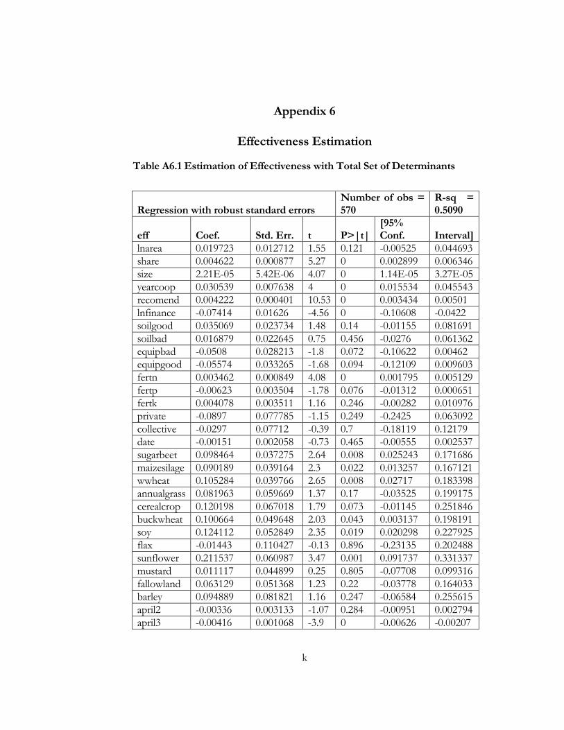
k
Appendix 6
Effectiveness Estimation
Table A6.1 Estimation of Effectiveness with Total Set of Determinants
Regression with robust standard errors Number of obs = 570
R-sq = 0.5090
eff Coef. Std. Err. t P>|t| [95% Conf. Interval]
lnarea 0.019723 0.012712 1.55 0.121 -0.00525 0.044693 share 0.004622 0.000877 5.27 0 0.002899 0.006346 size 2.21E-05 5.42E-06 4.07 0 1.14E-05 3.27E-05 yearcoop 0.030539 0.007638 4 0 0.015534 0.045543 recomend 0.004222 0.000401 10.53 0 0.003434 0.00501 lnfinance -0.07414 0.01626 -4.56 0 -0.10608 -0.0422 soilgood 0.035069 0.023734 1.48 0.14 -0.01155 0.081691 soilbad 0.016879 0.022645 0.75 0.456 -0.0276 0.061362 equipbad -0.0508 0.028213 -1.8 0.072 -0.10622 0.00462 equipgood -0.05574 0.033265 -1.68 0.094 -0.12109 0.009603 fertn 0.003462 0.000849 4.08 0 0.001795 0.005129 fertp -0.00623 0.003504 -1.78 0.076 -0.01312 0.000651 fertk 0.004078 0.003511 1.16 0.246 -0.00282 0.010976 private -0.0897 0.077785 -1.15 0.249 -0.2425 0.063092 collective -0.0297 0.07712 -0.39 0.7 -0.18119 0.12179 date -0.00151 0.002058 -0.73 0.465 -0.00555 0.002537 sugarbeet 0.098464 0.037275 2.64 0.008 0.025243 0.171686 maizesilage 0.090189 0.039164 2.3 0.022 0.013257 0.167121 wwheat 0.105284 0.039766 2.65 0.008 0.02717 0.183398 annualgrass 0.081963 0.059669 1.37 0.17 -0.03525 0.199175 cerealcrop 0.120198 0.067018 1.79 0.073 -0.01145 0.251846 buckwheat 0.100664 0.049648 2.03 0.043 0.003137 0.198191 soy 0.124112 0.052849 2.35 0.019 0.020298 0.227925 flax -0.01443 0.110427 -0.13 0.896 -0.23135 0.202488 sunflower 0.211537 0.060987 3.47 0.001 0.091737 0.331337 mustard 0.011117 0.044899 0.25 0.805 -0.07708 0.099316 fallowland 0.063129 0.051368 1.23 0.22 -0.03778 0.164033 barley 0.094889 0.081821 1.16 0.247 -0.06584 0.255615 april2 -0.00336 0.003133 -1.07 0.284 -0.00951 0.002794 april3 -0.00416 0.001068 -3.9 0 -0.00626 -0.00207

l
may1 0.002069 0.001244 1.66 0.097 -0.00037 0.004513 may2 0.00386 0.001639 2.36 0.019 0.000641 0.00708 may3 -0.01285 0.003302 -3.89 0 -0.01934 -0.00637 june1 -0.00368 0.001373 -2.68 0.008 -0.00637 -0.00098 june2 -0.0015 0.000522 -2.87 0.004 -0.00253 -0.00047 june3 -0.00965 0.001576 -6.12 0 -0.01275 -0.00655 july1 -0.00134 0.001334 -1.01 0.315 -0.00396 0.001278 july2 3.35E-05 0.001089 0.03 0.975 -0.00211 0.002173 lndensity 0.142863 0.131365 1.09 0.277 -0.11518 0.40091 _cons 0.971245 0.269065 3.61 0 0.442705 1.499786
. ovtest Ramsey RESET test using powers of the fitted values of eff Ho: model has no omitted variables F(3, 570) = 1.65 Prob > F = 0.1763 Table A.6 Estimation of Effectiveness with the Set of Significant
Determinants
Obs: 587 R-square
=0.3393
eff Coef. Std. Err. p-value
lnarea .0212708* .0132789 0.110
share .0031674*** .0009297 0.001
size .0000241*** 4.28e-06 0.000
yearcoop .0235336*** .0071652 0.001
recomend .0050828*** .0004058 0.000
lnfinance -.0758796*** .0160802 0.000
soilgood .0665511** .0273703 0.015
soilbad .0606597*** .0209758 0.004
equipbad -.0720171** .0299393 0.016
equipgood -.105199*** .0323196 0.001
fertn .0035368*** .0013344 0.008
fertp -.0069362* .0036582 0.058
fertk .0025293 .0032758 0.440
_cons .7076745*** .1767917 0.000

m
Appendix 7
Functional Form Specification MWD Test
Test description (from Gujarati, 1995, pp. 265-266):
H0: Linear Model: Y is a linear function of regressors.
H1: Log-linear Model: lnY is a linear function of logs of X’s.
1. Obtain estimated Yf from the linear regression.
2. Obtain estimated lnf from the log-linear regression.
3. Obtain z1=lnYf-lnf.
4. Regress Y on X’s and z1. Reject H0 if the coefficient of z1 is statistically significant.
5. Obtain z2=exp(lnf)-Yf.
6. Regress lnY on log of X’s and z2. Reject H1 if the coefficient of z2 is statistically significant.
Estimation Results:
Regression with robust standard errors Number of obs = 574
F( 34, 539) = 24.89
Prob > F = 0.0000
R-squared = 0.5381
------------------------------------------------------------------------------
| Robust
netyield | Coef. Std. Err. t P>|t| [95% Conf. Interval]
-------------+----------------------------------------------------------------
area | .0015449 .0006374 2.42 0.016 .0002929 .0027969
share | .0084062 .0041566 2.02 0.044 .0002411 .0165712
age | .00893 .0048169 1.85 0.064 -.0005322 .0183923
size | .000039 .0000203 1.92 0.055 -7.99e-07 .0000789

n
yearcoop | .1493582 .0343893 4.34 0.000 .0818048 .2169116
recomend | .0264786 .0019527 13.56 0.000 .0226426 .0303145
finance | -1.16e-06 4.64e-07 -2.49 0.013 -2.07e-06 -2.44e-07
soilgood | .5172026 .1173049 4.41 0.000 .2867717 .7476334
soilbad | -.0902376 .0944852 -0.96 0.340 -.275842 .0953669
april3 | -.0190301 .0041847 -4.55 0.000 -.0272503 -.0108098
may1 | .0131779 .0054039 2.44 0.015 .0025626 .0237931
may2 | .0350728 .0067775 5.17 0.000 .0217593 .0483863
may3 | -.0731985 .0151251 -4.84 0.000 -.1029099 -.0434871
june1 | -.0272197 .0057033 -4.77 0.000 -.0384231 -.0160164
june2 | -.0047391 .0021878 -2.17 0.031 -.0090368 -.0004414
june3 | -.0515552 .0067187 -7.67 0.000 -.0647532 -.0383571
july1 | -.014249 .0053712 -2.65 0.008 -.0247999 -.003698
equipbad | -.0964377 .0926582 -1.04 0.298 -.2784533 .0855778
sugarbeet | .644617 .1433059 4.50 0.000 .3631104 .9261237
maizesilage | .5454796 .1523788 3.58 0.000 .2461506 .8448086
wwheat | .5410445 .157912 3.43 0.001 .2308461 .8512428
annualgrass | .4780811 .2561969 1.87 0.063 -.0251857 .9813479
cerealcrop | .5384722 .2225268 2.42 0.016 .1013462 .9755983
buckwheat | .4707698 .1991073 2.36 0.018 .0796484 .8618913
soy | .9390775 .2428178 3.87 0.000 .4620924 1.416063
flax | -.5051056 .2208463 -2.29 0.023 -.9389305 -.0712807
sunflower | .9364736 .239938 3.90 0.000 .4651454 1.407802
mustard | -.000224 .1636386 -0.00 0.999 -.3216717 .3212236
fallowland | .4197261 .202352 2.07 0.039 .0222309 .8172212
barley | .3367543 .3506188 0.96 0.337 -.3519924 1.025501
fertn | .0122137 .0041878 2.92 0.004 .0039873 .02044
fertp | -.0058126 .0180226 -0.32 0.747 -.0412158 .0295906
fertk | .0074797 .0178681 0.42 0.676 -.0276199 .0425793
z1 | -.9967038 .3100932 -3.21 0.001 -1.605843 -.3875645
_cons | .5791553 .5033586 1.15 0.250 -.4096297 1.56794
------------------------------------------------------------------------------
. reg lnnetyield lnarea share age size yearcoop recomend lnfinance soilgood
soilbad april3 may1 m> ay2 may3 june1 june2 june3 july1 equipbad sugarbeet
maizesilage wwheat annualgrass cerealcrop buckwheat soy flax sunflower mustard
fallowland barley fertn fertp fertk z2, robust
Regression with robust standard errors Number of obs = 570
F( 34, 535) = 32.42
Prob > F = 0.0000
R-squared = 0.6185
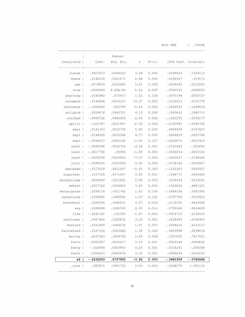
o
Root MSE = .34348
------------------------------------------------------------------------------
| Robust
lnnetyield | Coef. Std. Err. t P>|t| [95% Conf. Interval]
-------------+----------------------------------------------------------------
lnarea | .0827013 .0268325 3.08 0.002 .0299914 .1354113
share | .0149139 .0021671 6.88 0.000 .0106567 .019171
age | .0079819 .0022085 3.61 0.000 .0036435 .0123203
size | .0000494 8.20e-06 6.02 0.000 .0000333 .0000655
yearcoop | .0242482 .015917 1.52 0.128 -.0070194 .0555157
recomend | .0145844 .0010147 14.37 0.000 .0125912 .0165776
lnfinance | -.1904585 .033799 -5.64 0.000 -.2568535 -.1240634
soilgood | .2024678 .0490751 4.13 0.000 .1060643 .2988712
soilbad | -.0990726 .0484904 -2.04 0.042 -.1943275 -.0038177
april3 | -.013787 .0021947 -6.28 0.000 -.0180983 -.0094756
may1 | .0141193 .0023739 5.95 0.000 .0094559 .0187827
may2 | .0144309 .0030284 4.77 0.000 .0084819 .0203798
may3 | -.0096627 .0063145 -1.53 0.127 -.0220671 .0027416
june1 | -.0089346 .0026724 -3.34 0.001 -.0141842 -.003685
june2 | -.0017756 .00096 -1.85 0.065 -.0036614 .0001102
june3 | -.0205536 .0029063 -7.07 0.000 -.0262627 -.0148445
july1 | -.0089026 .0025004 -3.56 0.000 -.0138145 -.0039907
equipbad | -.0373018 .0411597 -0.91 0.365 -.1181563 .0435527
sugarbeet | .3157108 .0971457 3.25 0.001 .1248771 .5065445
maizesilage | .3026808 .1011691 2.99 0.003 .1039434 .5014181
wwheat | .3017162 .1004963 3.00 0.003 .1043004 .4991321
annualgrass | .2289118 .1411762 1.62 0.106 -.0484158 .5062395
cerealcrop | .2208056 .1499566 1.47 0.141 -.0737704 .5153816
buckwheat | .2269336 .1096631 2.07 0.039 .0115105 .4423568
soy | .3286898 .1286765 2.55 0.011 .0759168 .5814629
flax | -.2641141 .141395 -1.87 0.062 -.5418715 .0136433
sunflower | .3987462 .1200872 3.32 0.001 .1628459 .6346465
mustard | .2032455 .1064276 1.91 0.057 -.0058216 .4123127
fallowland | .2167318 .1563482 1.39 0.166 -.0903998 .5238634
barley | .4257263 .1608758 2.65 0.008 .1097005 .7417521
fertn | .0052397 .0016417 3.19 0.001 .0020148 .0084645
fertp | -.020854 .0063963 -3.26 0.001 -.0334191 -.008289
fertk | .0204415 .0060974 3.35 0.001 .0084638 .0324192
z2 | -.2232293 .0737955 -3.02 0.003 -.3681939 -.0782648
_cons | .802872 .3961723 2.03 0.043 .0246279 1.581116
------------------------------------------------------------------------------

p
Appendix 8
Endogeneity Check
Table A7.1 Estimation of Net Yield for Farms, Operating at Contract for One Year
Regression with robust standard errors if yearcoop==1
Number of obs = 216
R-sq = 0.6339
lnnetyield Coef. Std. Err. t P>|t| [95% Conf. Interval]
lnarea 0.022995 0.045238 0.51 0.612 -0.06626 0.112251
share 0.011436*** 0.002787 4.1 0 0.005937 0.016935
age 0.010741*** 0.003294 3.26 0.001 0.004242 0.017241
size 4.45E-05*** 1.06E-05 4.21 0 2.37E-05 6.54E-05
date -0.00662 0.007144 -0.93 0.355 -0.02071 0.007475
recomend 0.013625*** 0.001309 10.41 0 0.011043 0.016207
lnfinance -0.09466** 0.046653 -2.03 0.044 -0.18671 -0.00262
soilgood 0.004355 0.111287 0.04 0.969 -0.21522 0.223925
soilbad -0.16997** 0.0822 -2.07 0.04 -0.33216 -0.00779
april3 -0.00607* 0.003376 -1.8 0.074 -0.01273 0.000588
may1 0.01013*** 0.003099 3.27 0.001 0.004015 0.016245
may2 -0.00407 0.011606 -0.35 0.726 -0.02696 0.018833
may3 -0.01429* 0.008452 -1.69 0.093 -0.03096 0.002389
june1 -0.00117 0.005347 -0.22 0.828 -0.01171 0.009383
june2 -0.00374*** 0.001206 -3.1 0.002 -0.00612 -0.00136
june3 -0.01749*** 0.00354 -4.94 0 -0.02448 -0.01051
july1 -0.00664** 0.003159 -2.1 0.037 -0.01287 -0.00041
equipbad -0.39742*** 0.097543 -4.07 0 -0.58988 -0.20497
equipgood -0.31766** 0.141528 -2.24 0.026 -0.59689 -0.03842
sugarbeet 0.087807 0.098296 0.89 0.373 -0.10613 0.281745
maizesilage -0.00792 0.107843 -0.07 0.942 -0.2207 0.204853
wwheat 0.098808 0.100733 0.98 0.328 -0.09994 0.297556
annualgrass 0.015035 0.212339 0.07 0.944 -0.40391 0.433983
cerealcrop -0.45798*** 0.122796 -3.73 0 -0.70026 -0.21571
buckwheat -0.08166 0.119795 -0.68 0.496 -0.31802 0.154694
soy 0.038899 0.129713 0.3 0.765 -0.21703 0.294824
sunflower -0.05547 0.112584 -0.49 0.623 -0.2776 0.166655
fallowland 0.002602 0.228811 0.01 0.991 -0.44884 0.454048
barley 0.015122 0.081478 0.19 0.853 -0.14564 0.17588
fertn 0.005225* 0.003229 1.62 0.107 -0.00115 0.011596
fertp -0.00856 0.007568 -1.13 0.26 -0.02349 0.006373
fertk 0.006381 0.006662 0.96 0.339 -0.00676 0.019525
_cons 0.662004 0.627239 1.06 0.293 -0.57555 1.899553

q
Table A7.2 Estimation of Effectiveness for Farms, Operating at Contract for One Year
Regression with robust standard errors if yearcoop==1
Number of obs = 229
R-sq = 0.2957
eff Coef. Std. Err. t P>|t| [95% Conf. Interval]
share 0.002747 0.001414 1.94 0.053 -0.00004 0.005535
size 1.84E-05 5.39E-06 3.4 0.001 7.73E-06 0.000029
recomend 0.003939 0.000552 7.13 0 0.00285 0.005027
lnfinance -0.02907 0.022678 -1.28 0.201 -0.07377 0.015619
soilgood 0.102072 0.048082 2.12 0.035 0.007312 0.196832
soilbad 0.097256 0.029281 3.32 0.001 0.039548 0.154964
equipbad -0.08328 0.062902 -1.32 0.187 -0.20725 0.040687
equipgood -0.20771 0.075841 -2.74 0.007 -0.35718 -0.05824
_cons 0.409136 0.257843 1.59 0.114 -0.09902 0.917295
reg finance yield_1, robust Regression with robust standard errors Number of obs = 105 F( 1, 103) = 0.30 Prob > F = 0.5840 R-squared = 0.0029 Root MSE = 1.4e+05 ---------------------------------------------------------------------------------------------- | Robust finance | Coef. Std. Err. t P>|t| [95% Conf. Interval] -------------+------------------------------------------------------------------------------- yield_1 | -8906.044 16212.76 -0.55 0.584 -41060.23 23248.15 _cons | 142513.5 73045.18 1.95 0.054 -2354.401 287381.4 ---------------------------------------------------------------------------------------------- . corr area_total yield_1 (obs=111) | area_t~l yield_1 -------------+------------------ area_total | 1.0000 yield_1 | 0.1646 1.0000

r
Appendix 9
Farms’ Fixed Effect
.Table A8.1 Regression of Gross Barley Yield on Factors with Inclusion of Farm Specific Effect Regression with robust standard errors
Number of obs = 570
R-sq = 0.9825
lnyield Coef. Std. Err. t P>|t| [95% Conf. Interval]
private 0.172028 0.087245 1.97 0.05 0.000363 0.343694
collective 0.134599 0.158429 0.85 0.396 -0.17713 0.446328
recomend 0.00051 0.001177 0.43 0.665 -0.0018 0.002825
date -0.00111 0.000976 -1.14 0.256 -0.00303 0.00081
lndensity 0.535753 0.191897 2.79 0.006 0.158172 0.913334
soilbad 0.002206 0.010566 0.21 0.835 -0.01858 0.022997
soilgood 0.020437 0.031767 0.64 0.52 -0.04207 0.082942
sugarbeet 0.00096 0.006135 0.16 0.876 -0.01111 0.013032
maizesilage -0.00573 0.006044 -0.95 0.344 -0.01762 0.006163
wwheat 0.002659 0.008374 0.32 0.751 -0.01382 0.019134
annualgrass 0.002019 0.010135 0.2 0.842 -0.01792 0.021961
cerealcrop 0.008194 0.011282 0.73 0.468 -0.014 0.030391
soy 0.003933 0.011669 0.34 0.736 -0.01903 0.026893
flax -0.20722 0.007441 -27.85 0 -0.22186 -0.19258
rye -0.004 0.009729 -0.41 0.681 -0.02314 0.015145
may2 -0.00769 0.004656 -1.65 0.1 -0.01685 0.001473
july1 -0.0007 0.004004 -0.18 0.861 -0.00858 0.007177
lnarea 0.00247 0.004505 0.55 0.584 -0.00639 0.011334
equipgood 0.051353 0.037263 1.38 0.169 -0.02197 0.124673
var367 0.371987 0.140184 2.65 0.008 0.096158 0.647816
var366 -0.21792 0.193433 -1.13 0.261 -0.59852 0.162686
var365 -0.26951 0.150306 -1.79 0.074 -0.56525 0.026239
var364 -0.383 0.138836 -2.76 0.006 -0.65617 -0.10982
var363 -0.12445 0.191575 -0.65 0.516 -0.5014 0.252495
var362 0.167818 0.187219 0.9 0.371 -0.20056 0.536194
var360 0.07812 0.160214 0.49 0.626 -0.23712 0.39336
var359 -0.05722 0.192148 -0.3 0.766 -0.43529 0.32086
var358 -0.24048 0.162377 -1.48 0.14 -0.55998 0.079017
var258 -0.18096 0.158884 -1.14 0.256 -0.49358 0.131665
var257 -0.18477 0.161378 -1.14 0.253 -0.5023 0.132762
var256 -0.11413 0.173131 -0.66 0.51 -0.45478 0.22653
var255 0.010378 0.028653 0.36 0.717 -0.046 0.066755

s
var253 -0.1662 0.05802 -2.86 0.004 -0.28036 -0.05203
var252 -0.36508 0.187615 -1.95 0.053 -0.73424 0.004071
var251 0.162682 0.183442 0.89 0.376 -0.19826 0.523627
var250 0.250832 0.207563 1.21 0.228 -0.15757 0.659238
var249 -0.08439 0.147572 -0.57 0.568 -0.37475 0.205979
var248 0.090015 0.150508 0.6 0.55 -0.20613 0.386159
var247 -0.03284 0.094953 -0.35 0.73 -0.21967 0.153991
var246 -0.00447 0.170062 -0.03 0.979 -0.33909 0.330145
var245 -0.08861 0.154353 -0.57 0.566 -0.39232 0.215094
var244 0.109971 0.153184 0.72 0.473 -0.19144 0.411379
var243 -0.22903 0.098467 -2.33 0.021 -0.42277 -0.03528
var242 -0.3009 0.166656 -1.81 0.072 -0.62881 0.027017
var241 -0.0377 0.155902 -0.24 0.809 -0.34445 0.269057
var240 -0.121 0.09236 -1.31 0.191 -0.30273 0.060731
var239 -0.08257 0.195286 -0.42 0.673 -0.46682 0.301683
var238 -0.32004 0.133663 -2.39 0.017 -0.58303 -0.05704
var237 -0.44724 0.132472 -3.38 0.001 -0.70789 -0.18658
var236 -0.13082 0.133429 -0.98 0.328 -0.39336 0.13172
var235 -0.32978 0.206937 -1.59 0.112 -0.73695 0.077397
var234 -0.43231 0.0439 -9.85 0 -0.51868 -0.34593
var233 0.050742 0.101028 0.5 0.616 -0.14804 0.249527
var232 0.013199 0.136848 0.1 0.923 -0.25607 0.282465
var231 -0.12416 0.208908 -0.59 0.553 -0.53521 0.286891
var230 0.236665 0.207301 1.14 0.254 -0.17123 0.644556
var229 -0.0613 0.133942 -0.46 0.648 -0.32485 0.202245
var228 0.087759 0.118963 0.74 0.461 -0.14632 0.321832
var227 0.135505 0.118284 1.15 0.253 -0.09723 0.368243
var226 0.080747 0.162602 0.5 0.62 -0.23919 0.400685
var225 -0.00226 0.090741 -0.02 0.98 -0.1808 0.176285
var224 0.284023 0.162399 1.75 0.081 -0.03552 0.603563
var223 -0.11342 0.090551 -1.25 0.211 -0.2916 0.064746
var222 -0.03006 0.087328 -0.34 0.731 -0.20189 0.141769
var221 0.316168 0.131006 2.41 0.016 0.058398 0.573939
var220 0.196679 0.163088 1.21 0.229 -0.12422 0.517575
var219 0.295797 0.161749 1.83 0.068 -0.02246 0.614057
var218 0.243926 0.146368 1.67 0.097 -0.04407 0.531923
var217 0.09683 0.076981 1.26 0.209 -0.05464 0.2483
var216 -0.38904 0.104561 -3.72 0 -0.59477 -0.1833
var215 0.101442 0.10466 0.97 0.333 -0.10449 0.307373
var214 -0.76119 0.071747 -10.61 0 -0.90236 -0.62002
var213 -0.63982 0.106523 -6.01 0 -0.84941 -0.43022
var212 0.027306 0.117302 0.23 0.816 -0.2035 0.258112
var211 0.162293 0.254821 0.64 0.525 -0.3391 0.663683

t
var210 -0.07189 0.079462 -0.9 0.366 -0.22824 0.084463
var209 -0.07645 0.078537 -0.97 0.331 -0.23098 0.078078
var208 0.168836 0.07895 2.14 0.033 0.013492 0.32418
var207 0.154084 0.198228 0.78 0.438 -0.23595 0.544122
var206 0.127956 0.198039 0.65 0.519 -0.26171 0.517622
var205 -0.18886 0.19782 -0.95 0.34 -0.5781 0.200371
var204 0.304783 0.217181 1.4 0.162 -0.12255 0.732112
var135 -0.0122 0.215122 -0.06 0.955 -0.43547 0.411083
var134 -0.00286 0.217316 -0.01 0.99 -0.43046 0.424733
var133 -0.21846 0.215671 -1.01 0.312 -0.64282 0.205895
var132 0.300371 0.217064 1.38 0.167 -0.12673 0.727471
var131 0.017673 0.21487 0.08 0.935 -0.40511 0.440456
var130 0.153918 0.215279 0.71 0.475 -0.26967 0.577506
var129 0.407337 0.143774 2.83 0.005 0.124444 0.690231
var128 -0.16607 0.143373 -1.16 0.248 -0.44817 0.116039
var127 0.022872 0.213891 0.11 0.915 -0.39798 0.443727
var126 0.033548 0.169289 0.2 0.843 -0.29955 0.366645
var125 0.166227 0.215458 0.77 0.441 -0.25771 0.590167
var124 -0.24918 0.178593 -1.4 0.164 -0.60058 0.102225
var123 -0.06933 0.216032 -0.32 0.748 -0.4944 0.35574
var122 -0.0202 0.141111 -0.14 0.886 -0.29786 0.257447
var121 0.304909 0.216413 1.41 0.16 -0.12091 0.730728
var120 -0.02236 0.215165 -0.1 0.917 -0.44572 0.401005
var119 0.197405 0.140968 1.4 0.162 -0.07997 0.474776
var117 0.410893 0.21469 1.91 0.057 -0.01154 0.833322
var116 -0.05485 0.141924 -0.39 0.699 -0.3341 0.224401
var115 -0.21052 0.156358 -1.35 0.179 -0.51817 0.097137
var114 0.051642 0.214763 0.24 0.81 -0.37093 0.474214
var113 -0.0151 0.143979 -0.1 0.917 -0.29839 0.2682
var112 0.410272 0.212825 1.93 0.055 -0.00849 0.829031
var111 0.021751 0.209584 0.1 0.917 -0.39063 0.434132
var110 -0.11564 0.170736 -0.68 0.499 -0.45159 0.220301
var109 -0.04025 0.18052 -0.22 0.824 -0.39545 0.31494
var108 -0.10569 0.025975 -4.07 0 -0.1568 -0.05459
var107 -0.01087 0.12227 -0.09 0.929 -0.25145 0.229712
var106 -0.05807 0.03655 -1.59 0.113 -0.12999 0.013845
var105 -0.03861 0.157839 -0.24 0.807 -0.34917 0.27196
var104 0.08619 0.157802 0.55 0.585 -0.2243 0.396684
var103 0.185023 0.189355 0.98 0.329 -0.18756 0.557601
var102 -0.27534 0.076486 -3.6 0 -0.42583 -0.12484
var101 0.009601 0.114456 0.08 0.933 -0.2156 0.234806
var100 0.227847 0.18902 1.21 0.229 -0.14407 0.599767
var99 -0.14365 0.113452 -1.27 0.206 -0.36688 0.079582

u
var98 0.009472 0.052619 0.18 0.857 -0.09406 0.113007
var97 -0.09487 0.189237 -0.5 0.617 -0.46721 0.277481
var96 -0.01651 0.18909 -0.09 0.93 -0.38856 0.355551
var95 -0.00907 0.158667 -0.06 0.954 -0.32127 0.303121
var94 -0.1269 0.055407 -2.29 0.023 -0.23592 -0.01788
var93 0.211511 0.119281 1.77 0.077 -0.02319 0.44621
var92 -0.01761 0.057292 -0.31 0.759 -0.13033 0.095124
var91 0.275073 0.057434 4.79 0 0.162064 0.388082
var90 -0.13626 0.068288 -2 0.047 -0.27062 -0.0019
var89 0.255809 0.189876 1.35 0.179 -0.11779 0.629412
var88 -0.05175 0.073549 -0.7 0.482 -0.19647 0.092966
var87 -0.23714 0.162408 -1.46 0.145 -0.5567 0.082416
var86 -0.16196 0.091675 -1.77 0.078 -0.34235 0.018417
var85 -0.33024 0.187481 -1.76 0.079 -0.69913 0.038651
var84 -0.30642 0.188865 -1.62 0.106 -0.67804 0.065193
var83 0.058715 0.184553 0.32 0.751 -0.30441 0.421845
var82 0.104603 0.18799 0.56 0.578 -0.26529 0.474496
var81 -0.01914 0.16143 -0.12 0.906 -0.33677 0.298496
var79 -0.21771 0.15087 -1.44 0.15 -0.51457 0.079142
var78 -0.06283 0.162422 -0.39 0.699 -0.38241 0.25676
var77 0.100854 0.119071 0.85 0.398 -0.13343 0.335141
var76 0.00884 0.121375 0.07 0.942 -0.22998 0.247661
var74 0.103035 0.120763 0.85 0.394 -0.13458 0.34065
var73 -0.00578 0.074439 -0.08 0.938 -0.15225 0.140689
var72 0.214462 0.187486 1.14 0.254 -0.15444 0.583364
var71 0.345148 0.121277 2.85 0.005 0.106522 0.583775
var70 0.211407 0.191969 1.1 0.272 -0.16632 0.589129
var69 0.069687 0.092052 0.76 0.45 -0.11144 0.25081
var68 0.200392 0.163088 1.23 0.22 -0.1205 0.521286
var67 0.091447 0.100295 0.91 0.363 -0.1059 0.28879
var66 0.523397 0.166337 3.15 0.002 0.196109 0.850685
var65 0.207581 0.166147 1.25 0.212 -0.11933 0.534495
var64 0.075121 0.167131 0.45 0.653 -0.25373 0.403972
var63 0.174635 0.159844 1.09 0.275 -0.13988 0.489146
var62 -0.00682 0.162374 -0.04 0.967 -0.32631 0.31267
var61 0.077954 0.162783 0.48 0.632 -0.24234 0.39825
var60 0.017702 0.099284 0.18 0.859 -0.17765 0.213057
var59 0.160827 0.167672 0.96 0.338 -0.16909 0.490742
var58 0.109094 0.163258 0.67 0.504 -0.21214 0.430324
var57 -0.11337 0.12311 -0.92 0.358 -0.3556 0.128866
var56 0.081998 0.120548 0.68 0.497 -0.1552 0.319191
var55 0.201512 0.090477 2.23 0.027 0.023488 0.379535
var54 0.006122 0.162631 0.04 0.97 -0.31387 0.326117

v
var53 -0.07941 0.162436 -0.49 0.625 -0.39902 0.240206
var52 0.199221 0.162116 1.23 0.22 -0.11976 0.518204
var51 -0.10264 0.163416 -0.63 0.53 -0.42418 0.218902
var50 -0.021 0.162325 -0.13 0.897 -0.34039 0.298394
var49 -0.26758 0.090551 -2.95 0.003 -0.44575 -0.0894
var48 -0.09169 0.024155 -3.8 0 -0.13922 -0.04416
var47 0.050405 0.058975 0.85 0.393 -0.06564 0.166444
var46 -0.0934 0.128105 -0.73 0.466 -0.34547 0.158657
var45 0.197778 0.162891 1.21 0.226 -0.12273 0.518286
var44 0.035012 0.147922 0.24 0.813 -0.25604 0.326067
var43 0.265064 0.174329 1.52 0.129 -0.07795 0.608076
var42 -0.22259 0.236554 -0.94 0.347 -0.68804 0.242855
var41 0.316222 0.259802 1.22 0.224 -0.19497 0.827415
var40 0.3026 0.236185 1.28 0.201 -0.16212 0.767324
var39 0.258404 0.170234 1.52 0.13 -0.07655 0.593361
var38 0.144075 0.224492 0.64 0.521 -0.29764 0.585789
var37 -0.39776 0.117102 -3.4 0.001 -0.62817 -0.16734
var35 -0.30624 0.220336 -1.39 0.166 -0.73978 0.127299
var194 -0.10357 0.187572 -0.55 0.581 -0.47264 0.265506
var193 -0.0747 0.215788 -0.35 0.729 -0.49929 0.349884
var192 -0.25863 0.185421 -1.39 0.164 -0.62346 0.106213
var191 -0.01951 0.221547 -0.09 0.93 -0.45543 0.416413
var190 0.050882 0.192963 0.26 0.792 -0.3288 0.430559
var189 -0.15568 0.210527 -0.74 0.46 -0.56992 0.258559
var188 -0.0973 0.205856 -0.47 0.637 -0.50235 0.307748
var187 0.127961 0.238912 0.54 0.593 -0.34213 0.598049
var186 0.260728 0.196813 1.32 0.186 -0.12652 0.647982
var185 -0.25293 0.234433 -1.08 0.281 -0.7142 0.20835
var184 -0.02203 0.234377 -0.09 0.925 -0.48319 0.439137
var183 0.224975 0.188647 1.19 0.234 -0.14621 0.59616
var181 -0.17555 0.158561 -1.11 0.269 -0.48754 0.13644
var180 -0.01211 0.21591 -0.06 0.955 -0.43694 0.412717
var179 -0.32037 0.158126 -2.03 0.044 -0.6315 -0.00923
var178 -0.39546 0.155763 -2.54 0.012 -0.70194 -0.08898
var176 -0.1042 0.210159 -0.5 0.62 -0.51771 0.309319
var175 0.10194 0.220706 0.46 0.644 -0.33233 0.536206
var173 -0.08834 0.217556 -0.41 0.685 -0.5164 0.339732
var171 0.155578 0.303714 0.51 0.609 -0.44202 0.753173
var170 -0.02749 0.146943 -0.19 0.852 -0.31662 0.261635
var168 -0.37044 0.156173 -2.37 0.018 -0.67773 -0.06315
var167 0.168904 0.202622 0.83 0.405 -0.22978 0.567588
var166 0.117228 0.205754 0.57 0.569 -0.28762 0.522073
var165 -0.50999 0.069565 -7.33 0 -0.64687 -0.37311

w
var164 0.241673 0.18933 1.28 0.203 -0.13086 0.614203
var163 -0.09329 0.203291 -0.46 0.647 -0.49329 0.306712
var162 -0.27781 0.176621 -1.57 0.117 -0.62533 0.069712
var161 0.059996 0.160618 0.37 0.709 -0.25604 0.376031
var160 -0.09209 0.298503 -0.31 0.758 -0.67943 0.495256
var159 -0.34881 0.139604 -2.5 0.013 -0.6235 -0.07412
var158 -0.52796 0.091518 -5.77 0 -0.70804 -0.34789
var157 0.181256 0.107202 1.69 0.092 -0.02968 0.392189
var156 -0.18361 0.201724 -0.91 0.363 -0.58053 0.213308
var155 0.232226 0.228987 1.01 0.311 -0.21833 0.682786
var154 0.369417 0.154093 2.4 0.017 0.06622 0.672613
var153 0.134475 0.264731 0.51 0.612 -0.38642 0.655366
var151 0.399776 0.27472 1.46 0.147 -0.14077 0.940321
var152 0.418378 0.269472 1.55 0.122 -0.11184 0.948597
var150 0.27728 0.259579 1.07 0.286 -0.23347 0.788034
var149 0.501654 0.186494 2.69 0.008 0.134703 0.868604
var148 0.405695 0.252701 1.61 0.109 -0.09153 0.902915
var147 0.35433 0.216526 1.64 0.103 -0.07171 0.780371
var146 0.64871 0.290413 2.23 0.026 0.077288 1.220131
var145 0.47208 0.289497 1.63 0.104 -0.09754 1.041701
var144 0.482168 0.247562 1.95 0.052 -0.00494 0.969276
var143 0.50609 0.303159 1.67 0.096 -0.09041 1.102592
var142 0.027745 0.20529 0.14 0.893 -0.37619 0.431678
var141 0.070207 0.253761 0.28 0.782 -0.4291 0.569513
var140 0.393096 0.210178 1.87 0.062 -0.02046 0.806647
var139 0.137026 0.241112 0.57 0.57 -0.33739 0.611442
var138 0.093397 0.22625 0.41 0.68 -0.35178 0.538571
var137 0.449403 0.111301 4.04 0 0.230406 0.6684
var136 0.307676 0.21267 1.45 0.149 -0.11078 0.726131
var34 0.323329 0.21083 1.53 0.126 -0.0915 0.738164
var33 -0.1961 0.13108 -1.5 0.136 -0.45401 0.061816
var31 0.427806 0.226633 1.89 0.06 -0.01812 0.873734
var29 0.495746 0.302998 1.64 0.103 -0.10044 1.09193
var28 0.525352 0.260412 2.02 0.045 0.01296 1.037745
var27 0.480914 0.185909 2.59 0.01 0.115115 0.846712
var25 0.229116 0.281669 0.81 0.417 -0.3251 0.783334
var24 0.279796 0.303478 0.92 0.357 -0.31733 0.876926
var22 -0.05273 0.138762 -0.38 0.704 -0.32576 0.220301
var20 0.120011 0.21469 0.56 0.577 -0.30242 0.54244
var19 -0.51429 0.134335 -3.83 0 -0.77861 -0.24997
var36 -0.13816 0.195897 -0.71 0.481 -0.52361 0.247293
var18 0.05738 0.140418 0.41 0.683 -0.21891 0.333671
var17 0.058048 0.140776 0.41 0.68 -0.21895 0.335042

x
var16 0.008185 0.140841 0.06 0.954 -0.26894 0.285308
var15 0.016207 0.214147 0.08 0.94 -0.40515 0.437566
var13 0.158703 0.141599 1.12 0.263 -0.11991 0.437316
var12 0.262255 0.217655 1.2 0.229 -0.16601 0.690518
var9 0.201913 0.207607 0.97 0.332 -0.20658 0.610405
var8 -0.02267 0.132826 -0.17 0.865 -0.28402 0.238685
var7 -0.01311 0.138096 -0.09 0.924 -0.28483 0.258612
var5 0.312798 0.156274 2 0.046 0.00531 0.620287
var4 0.102772 0.215513 0.48 0.634 -0.32128 0.52682
var3 -0.13151 0.183387 -0.72 0.474 -0.49235 0.229322
var2 -0.09612 0.126901 -0.76 0.449 -0.34582 0.153568
_cons 0.551976 0.223288 2.47 0.014 0.112631 0.991322
Table A8.2 Regression of Effectiveness on Factors with Inclusion of Farm Specific Effect Regression with robust standard errors
Number of obs = 569
R-sq = 0.9338
eff Coef. Std. Err. t P>|t| [95% Conf. Interval]
share 0.006624 0.004948 1.34 0.182 -0.00311 0.01636
size 1.69E-06 7.73E-05 0.02 0.983 -0.00015 0.000154
yearcoop 0.07309 0.05148 1.42 0.157 -0.0282 0.174375
recomend 0.008853 0.00274 3.23 0.001 0.003462 0.014244
lnfinance -0.11083 0.118407 -0.94 0.35 -0.34379 0.122132
soilgood 0.027531 0.016587 1.66 0.098 -0.0051 0.060165
soilbad -0.00516 0.029647 -0.17 0.862 -0.06349 0.053169
equipbad 0.011339 0.031087 0.36 0.716 -0.04982 0.072503
equipgood -0.04693 0.089402 -0.52 0.6 -0.22283 0.128964
fertn -0.00435 0.002411 -1.8 0.072 -0.00909 0.000394
Fertp -0.00142 0.001482 -0.96 0.337 -0.00434 0.001492
Fertk 0.004768 0.002791 1.71 0.089 -0.00072 0.010258
var367 -0.01005 0.118016 -0.09 0.932 -0.24225 0.222142
var366* 0.326365 0.203333 1.61 0.109 -0.07369 0.726417
var365 0.07153 0.161902 0.44 0.659 -0.24701 0.390068
var364 0.2003 0.213481 0.94 0.349 -0.21972 0.620317
var363** 0.34172 0.156185 2.19 0.029 0.03443 0.649011
var362 -0.05957 0.22329 -0.27 0.79 -0.49889 0.379747
var361 0.327865 0.535646 0.61 0.541 -0.72601 1.381735
var360 -0.01369 0.147182 -0.09 0.926 -0.30327 0.275884
var359 0.124169 0.153021 0.81 0.418 -0.1769 0.425235
var358* 0.390738 0.248236 1.57 0.116 -0.09766 0.879135
var258 0.09358 0.200295 0.47 0.641 -0.3005 0.487655

y
var257* 0.29751 0.210593 1.41 0.159 -0.11683 0.711846
var256 0.182175 0.180205 1.01 0.313 -0.17237 0.536724
var255 0.61781 0.993802 0.62 0.535 -1.33747 2.573091
var254 0.02292 0.195888 0.12 0.907 -0.36248 0.408325
var253 -0.19222 0.163722 -1.17 0.241 -0.51434 0.129896
var252 0.098917 0.16468 0.6 0.548 -0.22509 0.422922
var251 -0.07287 0.222952 -0.33 0.744 -0.51152 0.365784
var250 0.033046 0.196794 0.17 0.867 -0.35414 0.420234
var249 -0.02697 0.376269 -0.07 0.943 -0.76727 0.71333
var248 -0.26446 0.221595 -1.19 0.234 -0.70044 0.171524
var247* 0.310544 0.21813 1.42 0.156 -0.11862 0.73971
var246 0.236745 0.185203 1.28 0.202 -0.12764 0.601126
var245 -0.13335 0.171007 -0.78 0.436 -0.4698 0.2031
var244 0.162037 0.194814 0.83 0.406 -0.22125 0.545328
var242 -0.1922 0.299952 -0.64 0.522 -0.78234 0.397952
var241* -0.26938 0.175398 -1.54 0.126 -0.61447 0.075715
var240 0.023619 0.187936 0.13 0.9 -0.34614 0.393378
var239 -0.07309 0.271873 -0.27 0.788 -0.60799 0.461817
var238* -0.37408 0.165895 -2.25 0.025 -0.70047 -0.04768
var237 -0.12127 0.19971 -0.61 0.544 -0.51419 0.271656
var236 0.000577 0.28596 0 0.998 -0.56204 0.563197
var235 0.612427 0.972824 0.63 0.529 -1.30158 2.526436
var234 0.221059 0.15545 1.42 0.156 -0.08479 0.526902
var233 -0.00325 0.165621 -0.02 0.984 -0.32911 0.322603
var232 0.235746 0.192848 1.22 0.222 -0.14368 0.615168
var231* -0.20685 0.138312 -1.5 0.136 -0.47897 0.065276
var230 -0.21196 0.159147 -1.33 0.184 -0.52508 0.101159
var229 0.064893 0.162977 0.4 0.691 -0.25576 0.385546
var228 0.00881 0.170319 0.05 0.959 -0.32629 0.343908
var227* 0.246236 0.154353 1.6 0.112 -0.05745 0.549922
var226 -0.09958 0.161136 -0.62 0.537 -0.41661 0.217453
var225 0.025127 0.146336 0.17 0.864 -0.26278 0.313039
var224 0.096636 0.158493 0.61 0.542 -0.2152 0.408466
var223 0.237532 0.169196 1.4 0.161 -0.09536 0.57042
var222 0.165151 0.153081 1.08 0.281 -0.13603 0.466334
var221** 0.287807 0.147667 1.95 0.052 -0.00273 0.578338
var220 0.238982 0.240828 0.99 0.322 -0.23484 0.712805
var219* 0.428446 0.151182 2.83 0.005 0.130998 0.725893
var218 -0.09278 0.134989 -0.69 0.492 -0.35836 0.172811
var217** 0.331441 0.173262 1.91 0.057 -0.00945 0.67233
var216*** 0.472755 0.157827 3 0.003 0.162233 0.783276
var215 0.062519 0.165142 0.38 0.705 -0.26239 0.387432
var214 0.022685 0.168127 0.13 0.893 -0.3081 0.35347

z
var213* 0.334635 0.235295 1.42 0.156 -0.1283 0.797572
var212** 0.233237 0.141551 1.65 0.1 -0.04526 0.511734
var211 0.137385 0.171078 0.8 0.423 -0.19921 0.473978
var210 0.013523 0.157313 0.09 0.932 -0.29599 0.323033
var209 -0.18621 0.196096 -0.95 0.343 -0.57203 0.199601
var208 -0.18016 0.203431 -0.89 0.376 -0.58041 0.220084
var207 0.278668 0.217593 1.28 0.201 -0.14944 0.706776
var206 -0.00101 0.15573 -0.01 0.995 -0.30741 0.305381
var205 -0.18837 0.167431 -1.13 0.261 -0.51779 0.141049
var204*** -0.5241 0.141507 -3.7 0 -0.80251 -0.24569
var135 -0.18067 0.162874 -1.11 0.268 -0.50112 0.139779
var134 -0.28141 0.23394 -1.2 0.23 -0.74168 0.178862
var133** -0.2492 0.126705 -1.97 0.05 -0.49849 8.98E-05
var132*** -0.41926 0.145045 -2.89 0.004 -0.70463 -0.13389
var131 -0.18272 0.160594 -1.14 0.256 -0.49868 0.133248
var130 -0.07812 0.16405 -0.48 0.634 -0.40088 0.244648
var129 -0.00968 0.185977 -0.05 0.959 -0.37559 0.356224
var128 0.09955 0.152129 0.65 0.513 -0.19976 0.398859
var127* -0.23347 0.142763 -1.64 0.103 -0.51436 0.047409
var126 0.111588 0.171776 0.65 0.516 -0.22638 0.449553
var125*** -0.34787 0.121763 -2.86 0.005 -0.58743 -0.1083
var124 0.071003 0.173874 0.41 0.683 -0.27109 0.413097
var123 0.077353 0.196002 0.39 0.693 -0.30828 0.462982
var122 -0.14138 0.155188 -0.91 0.363 -0.44671 0.163952
var121 -0.10335 0.133838 -0.77 0.441 -0.36667 0.159977
var120 0.07128 0.201241 0.35 0.723 -0.32466 0.467216
var119 -0.15892 0.135069 -1.18 0.24 -0.42467 0.106821
var117 -0.08699 0.137587 -0.63 0.528 -0.35769 0.183706
var116 -0.07728 0.156268 -0.49 0.621 -0.38473 0.230178
var115*** 0.53437 0.195508 2.73 0.007 0.149714 0.919027
var114 0.146588 0.175496 0.84 0.404 -0.1987 0.491872
var113 -0.15407 0.157334 -0.98 0.328 -0.46362 0.155485
var112 0.116481 0.195644 0.6 0.552 -0.26844 0.501406
var111 0.048469 0.191596 0.25 0.8 -0.32849 0.425429
var110 0.323989 0.240843 1.35 0.18 -0.14986 0.797842
var109 0.208707 0.229798 0.91 0.364 -0.24341 0.660828
var108* 0.46062 0.304983 1.51 0.132 -0.13943 1.060666
var107 -0.09538 0.167142 -0.57 0.569 -0.42423 0.233464
var106 0.265716 0.206796 1.28 0.2 -0.14115 0.672582
var105** 0.328766 0.19441 1.69 0.092 -0.05373 0.711262
var104* 0.233656 0.162974 1.43 0.153 -0.08699 0.554302
var103*** -0.42726 0.131796 -3.24 0.001 -0.68656 -0.16795
var102 0.141016 0.159792 0.88 0.378 -0.17337 0.455402

aa
var101 -0.04401 0.157556 -0.28 0.78 -0.35399 0.265979
var100* 0.336725 0.195213 1.72 0.086 -0.04735 0.720802
var99 0.184064 0.155514 1.18 0.237 -0.12191 0.490033
var98 0.149743 0.169849 0.88 0.379 -0.18443 0.483917
var97 0.190716 0.1419 1.34 0.18 -0.08847 0.469901
var96** 0.355491 0.155352 2.29 0.023 0.04984 0.661141
var95 0.273306 0.203688 1.34 0.181 -0.12745 0.674058
var94 0.058309 0.146711 0.4 0.691 -0.23034 0.34696
var93 0.012398 0.149172 0.08 0.934 -0.28109 0.30589
var92 0.009382 0.13868 0.07 0.946 -0.26347 0.282231
var91 0.01187 0.136206 0.09 0.931 -0.25611 0.279852
var90 0.289318 0.176114 1.64 0.101 -0.05718 0.635817
var89* -0.0203 0.202159 -0.1 0.92 -0.41804 0.377443
var88 0.162406 0.167847 0.97 0.334 -0.16783 0.492641
var87 0.057684 0.144193 0.4 0.689 -0.22601 0.34138
var86 0.184194 0.142746 1.29 0.198 -0.09666 0.465044
var85 0.053576 0.153652 0.35 0.728 -0.24873 0.355883
var84 0.177969 0.174641 1.02 0.309 -0.16563 0.521571
var83 0.1345 0.191028 0.7 0.482 -0.24134 0.510343
var82* 0.274426 0.145044 1.89 0.059 -0.01095 0.559797
var81* 0.307417 0.159111 1.93 0.054 -0.00563 0.620464
var80 0.06082 0.156597 0.39 0.698 -0.24728 0.36892
var79 0.069339 0.404434 0.17 0.864 -0.72638 0.865054
var78 -0.13213 0.155586 -0.85 0.396 -0.43824 0.173979
var76 -0.02233 0.15628 -0.14 0.886 -0.32981 0.285144
var74 -0.13674 0.127443 -1.07 0.284 -0.38748 0.114001
var73* 0.599078 0.412586 1.45 0.147 -0.21267 1.410831
var72 -0.08602 0.189934 -0.45 0.651 -0.45971 0.287668
var71 0.23565 0.128922 1.83 0.069 -0.018 0.489301
var70 0.212095 0.148415 1.43 0.154 -0.07991 0.504098
var69 0.232994 0.38961 0.6 0.55 -0.53355 0.999541
var68 0.115605 0.150266 0.77 0.442 -0.18004 0.411249
var67 0.16084 0.222125 0.72 0.47 -0.27619 0.597866
var66 -0.11101 0.192251 -0.58 0.564 -0.48926 0.267237
var65** 0.386436 0.210958 1.83 0.068 -0.02862 0.80149
var64 0.171084 0.239976 0.71 0.476 -0.30106 0.64323
var63 -0.06096 0.166931 -0.37 0.715 -0.38939 0.267471
var62 0.385187 0.178021 2.16 0.031 0.034936 0.735439
var61 0.167919 0.169106 0.99 0.321 -0.16479 0.50063
var60 -0.36225 0.150676 -2.4 0.017 -0.6587 -0.06579
var59 0.219796 0.250609 0.88 0.381 -0.27327 0.712863
var58 0.113078 0.188284 0.6 0.549 -0.25737 0.483521
var57 0.276253 0.20684 1.34 0.183 -0.1307 0.683205

bb
var56 0.082188 0.191096 0.43 0.667 -0.29379 0.458165
var55 0.192476 0.157476 1.22 0.223 -0.11735 0.502306
var54 0.07965 0.14753 0.54 0.59 -0.21061 0.369911
var53 -0.08249 0.135603 -0.61 0.543 -0.34929 0.184304
var52 0.051064 0.152716 0.33 0.738 -0.2494 0.351529
var51 0.400732 0.256367 1.56 0.119 -0.10366 0.905127
var50 -0.01365 0.158721 -0.09 0.932 -0.32593 0.298632
var49 0.212546 0.18462 1.15 0.25 -0.15069 0.575782
var48** 0.567676 0.25342 2.24 0.026 0.069077 1.066274
var47** 0.235931 0.352907 0.67 0.504 -0.45841 0.930267
var46 0.007159 0.248114 0.03 0.977 -0.481 0.495318
var45 -0.28857 0.141359 -2.04 0.042 -0.56669 -0.01045
var44 -0.03886 0.151236 -0.26 0.797 -0.33641 0.25869
var43** 0.362111 0.275524 1.31 0.19 -0.17998 0.904198
var42 0.314761 0.296352 1.06 0.289 -0.2683 0.897827
var41 -0.15703 0.386992 -0.41 0.685 -0.91843 0.604366
var40 0.01675 0.160989 0.1 0.917 -0.29999 0.333493
var39 -0.16709 0.273706 -0.61 0.542 -0.7056 0.371422
var38 -0.2209 0.1949 -1.13 0.258 -0.60436 0.162564
var37 0.038912 0.225739 0.17 0.863 -0.40522 0.483048
var35*** 0.591986 0.181945 3.25 0.001 0.234012 0.949959
var194** 0.473572 0.188108 2.52 0.012 0.103474 0.84367
var193 0.101295 0.162819 0.62 0.534 -0.21905 0.421637
var192** 0.49037 0.221662 2.21 0.028 0.054256 0.926483
var191 0.136086 0.183929 0.74 0.46 -0.22579 0.497962
var190* 0.420147 0.214963 1.95 0.052 -0.00279 0.843081
var188 0.163255 0.24114 0.68 0.499 -0.31118 0.637691
var187 0.294455 0.328133 0.9 0.37 -0.35114 0.940049
var186 0.286504 0.365409 0.78 0.434 -0.43243 1.005437
var185 0.302852 0.191604 1.58 0.115 -0.07412 0.679829
var184 0.142958 0.195717 0.73 0.466 -0.24211 0.528027
var183 0.089699 0.389446 0.23 0.818 -0.67653 0.855925
var182* 0.432096 0.239638 1.8 0.072 -0.03939 0.903579
var181* 0.337731 0.199086 1.7 0.091 -0.05397 0.729427
var180 0.186996 0.16804 1.11 0.267 -0.14362 0.51761
var179* 0.376591 0.217796 1.73 0.085 -0.05192 0.805098
var178** 0.523778 0.213332 2.46 0.015 0.104053 0.943504
var176 0.263772 0.208207 1.27 0.206 -0.14587 0.673415
var175 -0.018 0.17327 -0.1 0.917 -0.3589 0.322908
var173* 0.362556 0.202546 1.79 0.074 -0.03595 0.761061
var171 -0.19455 0.230008 -0.85 0.398 -0.64709 0.257982
var170* 0.376493 0.207262 1.82 0.07 -0.03129 0.784276
var168 0.158752 0.449266 0.35 0.724 -0.72517 1.042673

cc
var167 -0.21727 0.146271 -1.49 0.138 -0.50505 0.070519
var166* -0.33968 0.176892 -1.92 0.056 -0.68771 0.008352
var165 0.055494 0.248121 0.22 0.823 -0.43268 0.543667
var164 -0.10989 0.174645 -0.63 0.53 -0.4535 0.233724
var163 0.046018 0.14359 0.32 0.749 -0.23649 0.328528
var162 -0.19246 0.281383 -0.68 0.494 -0.74608 0.36115
var161 -0.07432 0.410885 -0.18 0.857 -0.88273 0.734084
var160 0.000143 0.20766 0 0.999 -0.40842 0.408708
var159 0.1635 0.186139 0.88 0.38 -0.20272 0.529725
var158 0.095524 0.229388 0.42 0.677 -0.35579 0.546838
var157 0.434945 0.446644 0.97 0.331 -0.44382 1.313706
var156 -0.21081 0.156412 -1.35 0.179 -0.51855 0.096926
var155 0.197425 0.184194 1.07 0.285 -0.16497 0.559821
var154*** -0.35681 0.148379 -2.4 0.017 -0.64875 -0.06488
var153 0.219326 0.21181 1.04 0.301 -0.19741 0.636058
var151 0.05135 0.274988 0.19 0.852 -0.48968 0.592382
var152 -0.02449 0.235112 -0.1 0.917 -0.48706 0.438089
var150 0.023835 0.328615 0.07 0.942 -0.62271 0.670377
var149 0.022797 0.181579 0.13 0.9 -0.33446 0.380049
var148 0.345154 0.183787 1.88 0.061 -0.01644 0.70675
var147 -0.09317 0.160848 -0.58 0.563 -0.40963 0.223294
var146* 0.248904 0.180795 1.38 0.17 -0.10681 0.604613
var145 -0.23103 0.336055 -0.69 0.492 -0.89221 0.430152
var144 -0.0481 0.25119 -0.19 0.848 -0.54231 0.446106
var143 -0.22476 0.181814 -1.24 0.217 -0.58248 0.132951
var142 0.201799 0.219249 0.92 0.358 -0.22957 0.633166
var141 -0.13563 0.187247 -0.72 0.469 -0.50403 0.232775
var140 -0.20437 0.163901 -1.25 0.213 -0.52684 0.118101
var139 -0.13413 0.17985 -0.75 0.456 -0.48798 0.219726
var138 0.034631 0.189568 0.18 0.855 -0.33834 0.407602
var137 -0.00505 0.444584 -0.01 0.991 -0.87976 0.869654
var136 0.291477 0.196333 1.48 0.139 -0.0948 0.677756
var34 -0.00363 0.270922 -0.01 0.989 -0.53666 0.529405
var33 0.055459 0.20419 0.27 0.786 -0.34628 0.457198
var31 0.063006 0.139496 0.45 0.652 -0.21145 0.33746
var29 -0.29112 0.234698 -1.24 0.216 -0.75289 0.170637
var28 -0.20405 0.226137 -0.9 0.368 -0.64897 0.240867
var27 -0.06466 0.348781 -0.19 0.853 -0.75087 0.62156
var25 0.196433 0.207662 0.95 0.345 -0.21214 0.605003
var24 -0.16464 0.238297 -0.69 0.49 -0.63349 0.3042
var22* 0.206259 0.143218 1.44 0.151 -0.07552 0.488036
var20 -0.2347 0.187086 -1.25 0.211 -0.60279 0.133385
var19** 0.54032 0.267107 2.02 0.044 0.014793 1.065846

dd
var36 0.128484 0.171369 0.75 0.454 -0.20868 0.465647
var18* -0.22314 0.139883 -1.6 0.112 -0.49835 0.052081
var17** -0.28969 0.14064 -2.06 0.04 -0.5664 -0.01298
var16 -0.19201 0.180003 -1.07 0.287 -0.54616 0.162145
var15 0.011933 0.131183 0.09 0.928 -0.24617 0.270032
var13 0.107334 0.158722 0.68 0.499 -0.20495 0.419616
var12 0.327684 0.197135 1.66 0.097 -0.06017 0.715542
var9 0.145261 0.405673 0.36 0.721 -0.65289 0.943413
var7 0.063978 0.194574 0.33 0.743 -0.31884 0.446797
var5 -0.22361 0.288626 -0.77 0.439 -0.79148 0.344251
var4 -0.14454 0.249067 -0.58 0.562 -0.63458 0.34549
var3 0.027263 0.276088 0.1 0.921 -0.51593 0.570459
var2 -0.32392 0.241548 -1.34 0.181 -0.79916 0.151319
_cons 0.610838 1.299295 0.47 0.639 -1.94549 3.167169