Chemical Geology 324-325 (2012) 28–45

Contents lists available at SciVerse ScienceDirect

Chemical Geology

j ourna l homepage: www.e lsev ie r .com/ locate /chemgeo

Research paper

Controls on organic carbon and molybdenum accumulation in Cretaceous marinesediments from the Cenomanian–Turonian interval including Oceanic Anoxic Event 2

Andrew W. Dale a,⁎, Stephen R. Meyers b, David R. Aguilera c,d, Sandra Arndt d, Klaus Wallmann a

a IFM-GEOMAR Leibniz Institute of Marine Sciences, Wischhofstrasse 1–3, 24148 Kiel, Germanyb University of Wisconsin-Madison, 1215 W. Dayton St., Madison, WI 53706, USAc DELTARES, Princetonlaan 6, 3508 TA Utrecht, Netherlandsd Department of Earth Sciences, Utrecht University, P.O. Box 80.021, 3508TA, Utrecht, Netherlands

⁎ Corresponding author. Tel.: +49 431 600 2291; faxE-mail address: adale@ifm-geomar.de (A.W. Dale).

0009-2541/$ – see front matter © 2011 Elsevier B.V. Alldoi:10.1016/j.chemgeo.2011.10.004

a b s t r a c t

a r t i c l e i n f o

Article history:Accepted 8 October 2011Available online 15 October 2011

Keywords:CretaceousOcean Anoxic Event 2ModelMolybdenumIronSediment

This study investigates the controls on organic carbon andmolybdenum(Mo) accumulation in sediments depos-itedwithin theWestern Interior Seaway across the Cenomanian–Turonian boundary interval (94.34–93.04 Ma)including Oceanic Anoxic Event 2 (OAE2). Carbon fluxes to the sediment–water interface (reflecting changes inprimary productivity) and bottom-water oxygen concentrations (reflecting preservation effects) are recon-structed fromfield data and used to constrain a benthicmodel that simulates the geochemistry of unconsolidatedsediments as they were deposited. The results show that increased availability of reactive iron prevents Mo se-questration as thiomolybdate (MoS42−) during OAE2 (O2~105 μM) by (i) inhibiting sulfate reduction, and (ii)buffering any free sulfide that becomes available. In the post-OAE2 period (O2~50 μM), Mo accumulation is fa-vored by a large reduction in iron flux. Importantly, this occurs in parallel with oxygenated bottom waters andhigh rates of aerobic carbon degradation in the surface sediments, implying that elevatedMo burial fluxes in an-cient marine facies do not necessarily reflect euxinic or even anoxic conditions within the water column. Ourfindings suggest that both an increase in production and preservation lead to enrichment in organic carbon intheWestern Interior Seaway.More generally, the results demonstrate that a careful consideration of the couplingbetween iron, carbon and oxygen cycles during the early stages of diagenesis is critical for interpreting geochem-ical proxies in modern and ancient settings.

© 2011 Elsevier B.V. All rights reserved.

1. Introduction

The Cretaceous period (145.5–65.5 Ma) was characterized bywarm climates and high eustatic sea level (Barron, 1983). The corre-sponding marine sedimentary record is punctuated by dark coloredfully- or partially-laminated facies enriched in organic carbon (OC)and trace metals known as black shales (Arthur and Sageman, 1994).Within these sequences, which were deposited over 104–105 yr time-scales, the δ13C values for OC andmarine carbonates show a positive ex-cursion, explained as regional to global scale perturbations in thecoupled ocean–atmosphere carbon cycle (Arthur et al., 1988). Multi-proxy data suggest that these sediments were deposited under watercolumn anoxia or even euxinia, conditions more generally describedas ocean anoxic events (OAE) (Schlanger and Jenkyns, 1976; Steinet al., 1986; Jenkyns, 2010).

Oneof themostwidely studied anoxic events is OAE2,which straddlesthe Cenomanian–Turonian (C–T) boundary interval (94.34–93.04 Ma).The extent of OC enrichment in OAE2 strata varies by region (Jenkyns,

: +49 431 600 2928.

rights reserved.

2010). For example, OC contents of 13 wt.% are observed in the deep-sea proto-North Atlantic, while 20 wt.% OC is preserved in continentalshelf sediments off the coast of Suriname (Hetzel et al., 2009; Kraalet al., 2010). These contents compare to ca. 2 wt.% on the continentalshelf in modern marine sediments and b1 wt.% in the deep sea (Seiteret al., 2005). Significantly higher contents of 10 wt.% or more are to befound in anoxic basins, upwelling areas and oxygen minimum zonesin the contemporary ocean which are generally seen as analogs ofOAEs (Algeo and Lyons, 2006). Yet these settings comprise a small sur-face area of the modern global ocean compared to the extensive natureof anoxia believed to characterize OAE2 (Arthur et al., 1987; Schlangeret al., 1987).

The factors leading to OC enrichment in ancient marine sedimentsare not well substantiated, and discussions often center on the dichoto-my of export production versus preservation (Demaison and Moore,1980; Pedersen and Calvert, 1990). On the one hand, sediments under-lying anoxic bottom waters are thought to better preserve OC becausethe rate of carbon degradation by anaerobic bacteria appears to beslower than that for aerobic bacteria, at least for less reactive OC frac-tions (Middelburg et al., 1993; Canfield, 1994; Moodley et al., 2005).This has led to the concept of oxygen exposure time (OET), that is,where OC degradation is enhanced when the residence time of OC in

29A.W. Dale et al. / Chemical Geology 324-325 (2012) 28–45

the oxic sediment layers increases (Hedges and Keil, 1995). However,Middelburg et al. (1993) caution that the perceived importance of oxy-gen could simply be a consequence of diagenetic maturity, wherebyaerobic respiration consumes themost reactive OC fractions, leaving be-hind the less reactivematerial for the anaerobicmicroorganisms.Mech-anistically, the relationship between OET and OC accumulation couldalso be attributed to changes in the rate of delivery of labile OC tosulfide-rich porewater, as hydrogen sulfide serves as control on organicmatter vulcanization, ‘hydrogenation’ and preservation (e.g., Hebting etal., 2006; Arndt et al., 2009). With regard to the production argument,higher rates of primary production and deposition of organic detritusmay simply enrich the sediment in OC. However, because anoxicsediments preferentially release phosphorus back to the water col-umn, the potential exists for a positive feedback between primaryproduction and benthic OC enrichment (Van Cappellen and Ingall,1994; Ingall and Jahnke, 1997). Consequently, higher levels of pro-duction and preservation are both possible drivers for OC enrich-ment during anoxic events; a fact that is not always obvious fromthe debate in the geological literature (Demaison and Moore, 1980;Pedersen and Calvert, 1990).

Key to interpreting measured data with regard to the extent towhich production and preservation processes may have developedat the start of anoxic events and their ultimate control on OC accumu-lation is a mechanistic understanding of the coupled physical and bio-geochemical processes occurring within the sediments themselves. Atransition towards anoxia at the start of the anoxic event would havebeen met by a shift from predominantly aerobic respiration of OC (c.f.the contemporary deep ocean) towards sulfate-based anaerobic res-piration (c.f. the contemporary silled basins and productive shelf set-tings). A thinner aerobic layer will lead to enhanced transport oflabile OC to the anaerobic sulfate reduction zone where preservationismore likely (Canfield, 1994; Tyson, 2001;Meyers et al., 2005; Burdige,2007). Preservationwill be further enhanced if bulk accumulation ratesalso increase simultaneously. Yet, too high sedimentation rates will di-lute the OC concentration to the point where OC enrichment is no lon-ger perceptible (Tyson, 2001). Paradoxically, the sediment carbonburial efficiency (CBE=burial flux∕deposition flux×100%) in thiscasewill be high because of the enhanced delivery flux to the sulfate re-duction zone (Burdige, 2007). On the other hand, OCwill be extensivelydegraded in sediments that accumulate very slowly under oxic bottomwaters due to the long residence time of particles in the oxic layer, lead-ing to a lowCBE. These coupled processes imply that to accurately inter-pret sedimentary proxy records, due considerationmust be given to thedynamic interplay between the major transport and biogeochemicalprocesses in sediments (Arndt et al., 2009).

An additional and widely-considered indicator for ocean anoxia isthe enrichment of trace metals in black shales (Sageman and Lyons,2003). Molybdenum (Mo) is currently of high interest in this regardbecause of the different geochemical speciation it exhibits under dif-ferent redox conditions. Dissolved molybdate (MoO4

2−) behaves con-servatively in oxic aquatic environments, yet undergoes quantitativesulfidization to dissolved thiomolybdate (MoOxS4-x2−) when hydrogensulfide ion (HS−) reaches a critical concentration threshold of ca.50–250 μM (Helz et al., 1996; Zheng et al., 2000). Tetrathiomolybdate(MoS42−) is immobilized through adsorption onto mineral phases andorganic substrates and eventually becomes buried to the sediment re-pository (Helz et al., 1996; Tribovillard et al., 2004). Consequently,Mo concentrations in black shales (101–102 ppm) tend to be at leastan order-of-magnitude larger than average crustal values (1–2 ppm)(Wedepohl, 1991) and they also show a degree of correlation withtheOC content in both contemporary (Algeo and Lyons, 2006;McManuset al., 2006) and ancient facies (Kolonic et al., 2005). This indicates thatthe controls on OC andMo accumulation ratesmay be related. However,the reductive dissolution of reactive iron by sulfide can dramaticallymodulate the concentration of free hydrogen sulfide in the pore-water (Jørgensen, 1977; Raiswell and Canfield, 1996) and prevent

formation of MoS42−. This sulfide sink can potentially limit the utilityof Mo as a paleoproxy (Meyers, 2007).

In this study, our prime objective is to quantify theprocesses control-lingOC andMoenrichment inmarine sediments fromOAE2.We employa numerical reaction-transport model that integrates physical processesand biogeochemical reactions into a quantitative framework. As a casestudy, we focus on the CretaceousWestern Interior Seaway— a shallow(300 m paleo-water depth) epicontinental water body linking the Bore-al Ocean to the north and the Tethys Ocean to the south in what is nowthe western USA. Specifically, we address the Bridge Creek LimestoneMember, which brackets the C–T boundary, including OAE2 and thepost-OAE2 period (94.34–93.04 Ma) (Sageman et al., 2006). Our ap-proach constitutes a new quantitative framework for the analysis ofdeep-time biogeochemical perturbations, and the results are of signifi-cance for the accurate interpretation of proxy records in both ancientand modern sediments.

2. Geological and paleoceanographic setting of the WIS

During the late C–T interval, high eustatic sea level and foreland basinsubsidence led to the development of theWestern Interior Seaway (WIS)in western North America (Kauffman, 1977). The WIS was a meridionalseaway that connected the high-latitude Boreal Ocean to the low-latitudeTethys Sea, with the Sevier Orogenic Belt lying to thewest (e.g. Kauffman,1977). Reconstructions ofwatermass dynamicswithin the seaway, basedon paleobiologic, sedimentologic, geochemical evidence and circulationmodeling (e.g. Slingerland et al., 1996; Kump and Slingerland, 1999;Fisher and Arthur, 2002), indicate a dynamic interplay between distinctBoreal and Tethyan water masses during the Cenomanian and Turonian.In summary, these studies suggest that the WIS hosted a cyclonic gyre,with Boreal surface water influx from the north and Tethyan surfacewater influx from the south. Turbulent mixing within the seaway likelyprohibited the development of a stable density stratification of thewater column (Kump and Slingerland, 1999).

The present study evaluates data from the USGS #1 Portland core(Sageman et al., 1997; Meyers et al., 2005), located in the central por-tion of the seaway, and composed of sediments deposited at approx-imately 300 m paleowater depth (Sageman and Arthur, 1994). At thislocation, the C–T boundary interval is predominantly composed ofrhythmically alternating decimeter-scale limestone and marlstonebeds, which constitute the Bridge Creek Limestone Member (Green-horn Formation) (Sageman et al., 1997). Individual beds of the BridgeCreek Limestone Member can be traced for over 1000 km (Elder et al.,1994). This basin-wide rhythmic sedimentation has been quantita-tively linked to an orbital driver (Sageman et al., 1997; Meyerset al., 2001; Meyers and Sageman, 2007), yielding a high-resolutionchronometer that permits detailed evaluation of geochemical fluxesthrough the C–T boundary interval, both during and immediately fol-lowing OAE2 (Meyers et al., 2001; 2005).

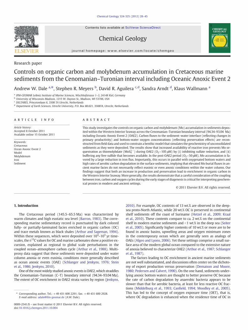
A selection of the Bridge Creek data fromMeyers et al. (2005) whichhave been smoothed with a 2 m moving average filter (Fig. 1) revealslarge secular changes inOC, Fe andMo concentrations and accumulationrates across the C–T interval. These rates are not spectacular comparedto other OAE2 sequences (e.g. Kolonic et al., 2005) and aremore compa-rable to those encountered in modern deep sea settings. However, thedata are unique because the OC and Mo accumulation rates are highestpost-OAE2,which suggests that ‘OAE2-like’ conditions in theWIS laggedbehind the global ocean. According to Meyers et al. (2005) and Meyers(2007), the elevated fluxes of reactive oxidized iron (i.e. iron oxide–hydroxides) relative to OC during OAE2 (Fig. 1e), perhaps enhancedby an additional (hydrothermal?) iron source decoupled from the detritalflux, had a strong influence on these trends. They hypothesized thatabundant reactive iron efficiently removed dissolved sulfide from sedi-mentary pore waters through oxidation reactions, effectively inhibitingmolybdate sulfidization. This hypothesis is analyzed in detail in the pre-sent study in the context of OC and Mo accumulation.

BCM

Sedimentationvelocity

0.6 0.8 112

3

4

5

6

7

8

9

10

11

Hei

ght (

m)

a

Fω BS-BCM

Bulk sedimentaccumulation rate

1.5 2 2.5

g cm-2 ky-1cm ky-1 g cm-2 ky-1 g cm-2 ky-1 g cm-2 ky-1

b

FC-BCM

OCaccumulation rate

0.02 0.04 0.06

c

FCa-BCM

CaCO3accumulation rate

1 1.5 2

d

FFe-BCM

Feaccumulation rate

0.01 0.02 0.03 0.04

e

FMo-BCM

Moaccumulation rate

5 10 15

f

FOLFrequency of

lamination

10 20 30 40 50 60%

g

OA

E2

po

st-OA

E2

94.34

94.11

93.99

93.89

94.24

93.78

93.64

93.49

93.35

93.19

93.01

Age

(Ma)

μg cm-2 ky-1

Fig. 1.Measured data from the Western Interior Seaway (black lines) represented with a 2 m moving average filter redrawn from Meyers et al. (2005). Height refers to relative spatiallocation within the Bridge Creek Limestone Member. (a) sediment burial velocity (ωBCM), (b) bulk sediment accumulation rate (FBS-BCM), (c) OC accumulation rate (FC-BCM), (d) calciumcarbonate accumulation rate (FCa-BCM), (e) iron accumulation rate (FFe-BCM), (f) molybdenum accumulation rate (FMo-BCM), and (g) frequency of lamination (FOL). The stippled area in (e)is the ‘excess’ ironflux decoupled from the local terrigenous (detrital) flux calculated fromTi accumulation (Meyers et al., 2001). The dashed horizontal lines indicate the separation of thedata into 15 distinct time intervals and the mean values of the data within each interval are shown by the white circles. The gray shaded area highlights the domain of OAE2. The C/Tboundary is located at 4.88 m height (Meyers et al., in press).

30 A.W. Dale et al. / Chemical Geology 324-325 (2012) 28–45

3. A model for Cretaceous sediments of the WIS

On the basis of identifiable changes in bulk sediment and carbonaccumulation rates, the data in Fig. 1 were subdivided into 15 distincttime intervals. It is our intention to use a model to simulate the OC, Feand Mo concentrations and accumulation rates for each of these timeintervals in the unconsolidated (porous) sediments as they werebeing deposited. This presents some complications since the sedi-ments are now fully lithified material. We thus use geochemicaldata measured in the strata to extract the necessary boundary condi-tions and parameters required to describe the changing conditions atthe sea floor over the C–T interval. In other words, 15 model simula-tions of the unconsolidated sediments of the Cretaceous WIS are per-formed, each having boundary conditions and parameters whichdiffer from one time interval to the next. Comparison of the modeloutput with the measured data in Fig. 1 will provide a quasi-validationthat the derived model forcing functions have been adequately de-scribed. The 15 time intervals are sufficiently long (>104 yr) so thateach of the simulations was run to steady state, that is, until there is notemporal change in the concentration–depth profiles (see Section 3.1).

The strategy outlined in this section proceeds as follows. First, weintroduce the model framework for simulating coupled reaction andtransport in unconsolidated (porous) marine sediments. We then de-scribe how key model boundary conditions and parameters for eachtime slice were extracted from the data in Fig. 1. We end this sectionby describing how the model can be used in conjunction with a sys-tem analysis to extract the factors controlling Mo and OC accumula-tion rates in Cretaceous sediments. In what follows, the subscripts‘cr’, ‘BCM’ and ‘co’ indicate that the corresponding parameters orboundary conditions apply to unconsolidated Cretaceous sediments,to consolidated Bridge Creek Limestone Member strata, or to contem-porary marine sediments, respectively.

3.1. Model set-up

3.1.1. Modeling coupled reaction and transportThemodel is designed to simulate the concentration profiles of aque-

ous, Ca(z), and solid species, Cs(z) in theupper 150 cmof Cretaceous sed-iments at a water depth characteristic of the WIS (300 m, Slingerlandet al., 1996; Meyers et al., 2005). Solutes considered are oxygen (O2),

sulfate (SO42−), total hydrogen sulfide (TH2S), molybdate (MoO4

2−)and ferrous iron (Fe2+) and solids considered are pelagic particulate or-ganic carbon deposited on the seafloor (OC, chemically defined as CH2O),reactive iron oxide–hydroxide (Fe(OH)3), iron sulfide (FeS) and thiomo-lybdate (MoS42−). In this paper, the term reactive iron refers to theiron oxide–hydroxide fraction. The speciation of dissolved sulfide isnot explicitly calculated and unless indicated ‘TH2S’ refers to ΣH2S+HS−+S2−. The one-dimensional mass-conservation equation (Berner,1980; Boudreau, 1997) was used to simulate concentrations along thevertical (depth) axis, z:

φ zð Þ⋅ ∂Ca zð Þ∂t ¼ ∂

∂z ⋅ φ zð Þ⋅ Dcr zð Þ þ Dbcr zð Þð Þ⋅ ∂Ca zð Þ∂z

� �

−∂ φ zð Þ⋅vcr zð Þ⋅Ca zð Þð Þ∂z þαcr zð Þ⋅ Ca 0ð Þ−Ca zð Þð Þ þ Σr zð Þ⋅φ zð Þ

ð1aÞ

1−φ zð Þð Þ⋅ ∂Cs zð Þ∂t ¼ ∂

∂z ⋅ 1−φ zð Þð Þ⋅Dbcr zð Þ⋅ ∂Cs zð Þ∂z

� �

−∂ 1−φ zð Þð Þ⋅ωcr zð Þ⋅Cs zð Þð Þ∂z þ Σr zð Þ⋅ 1−φ zð Þð Þ

ð1bÞ

where t is time, φ(z) is the sediment porosity and Σr is the sum of therates of change of concentration due to biogeochemical reactions. Themodel parameters are Dcr(z), Dbcr(z), ωcr(z), vcr(z) and αcr(z), whichrepresent the molecular diffusion coefficient of solutes in sediments,mixing by bioturbation, the burial velocity of solids, the burial velocityof porewater, and solute exchange bybioirrigation, respectively. Detailson how these parameters are estimated are described below. Solutesand solids are modeled as molar (mol L−1) and mass (weight %(wt.%)) concentrations. Model parameters and boundary conditionsare listed in Table 1.

3.1.2. Sediment porosityThe porosity of muddy marine sediments typically decreases fairly

rapidly in the surface layers (upper dm) due to compaction and thenshows a more attenuated decrease with increasing depth. The change

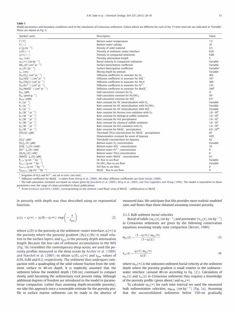
Table 1Model parameters and boundary conditions used in the simulation of Cretaceous sediments. Values which are different for each of the 15 time intervals are indicated as ‘Variable’.These are shown in Fig. 6.

Symbol (unit) Description Value

T (°C) Bottom water temperature 7.5S (−) Bottom water salinity 35ρ (g cm−3) Density of solid material 2.5φ(0) (−) Porosity at sediment–water interface 0.95φ(∞) (−) Porosity in compacted sediments 0.80zpor (cm) Porosity attenuation length 5ωcr(∞) (cm ky−1) Burial velocity in compacted sediments VariableDbcr(0) (cm2 yr−1) Surface bioturbation coefficient Variableαcr(0) (yr−1) Surface bioirrigation coefficient Variablea

zcr (cm) Mixing depth by animals VariableDW(O2) (cm2 yr−1) Diffusion coefficient in seawater for O2 402DW(SO4

2−) (cm2 yr−1) Diffusion coefficient in seawater for SO42− 197

DW(TH2S) (cm2 yr−1) Diffusion coefficient in seawater for TH2S 360DW(Fe2+) (cm2 yr−1) Diffusion coefficient in seawater for Fe2+ 132DW(MoO4

2−) (cm2 yr−1) Diffusion coefficient in seawater for MoO42− 184b

KO2 (μM) Half-saturation constant for O2 4c

KFe (μmol g−1) Half-saturation constant for Fe(OH)3 50c

KSO4 (mM) Half-saturation constant for SO42− 0.5c

k1 (yr−1) Rate constant for OC mineralization with O2 Variablek2 (yr−1) Rate constant for OC mineralization with Fe(OH)3 Variablek3 (yr−1) Rate constant for OC mineralization with SO4

2− Variablek4 (M−1 yr−1) Rate constant for ferrous iron oxidation with O2 1.0·108

k5 (M−1 yr−1) Rate constant for biological sulfide oxidation 1.0·108

k6 (M−1 yr−1) Rate constant for FeS precipitation 1.0·107

k7 (M−1 yr−1) Rate constant for chemical sulfide oxidation 1.0·103

k8 (M−1 yr−1) Rate constant for FeS oxidation with O2 1.0·106

k9 (M−1 yr−1) Rate constant for MoS42− precipitation 6.9·104d

[TH2S]* (μM) Threshold TH2S concentration for MoS42− precipitation 65τ Dimensionless constant for onset of hypoxia 0.05[O2]* (μM) Threshold concentration for hypoxia 62[O2]cr(0) (μM) Bottom water O2 concentration Variable[SO4

2−]cr(0) (mM) Bottom water SO42− concentration 10

[Fe2+]cr(0) (nM) Bottom water Fe2+ concentration 0[H2S]cr(0) (nM) Bottom water TH2S concentration 0[MoO4

2−]cr(0) (μM) Bottom water MoO42− concentration 0.1

FC-cr (g cm−2 ky−1) OC flux to sea floor VariableFFe-cr (g cm−2 ky−1) Fe(OH)3 flux to sea floor VariableFFeS-cr (g cm−2 ky−1) FeS flux to sea floor 0FMoS4-cr (μg cm−2 ky−1) MoS42− flux to sea floor 0

a Irrigation of H2S and Fe2+ are set to zero (see text).b Diffusion coefficient for MoO4

2− is taken from Zheng et al. (2000). All other diffusion coefficients are from Schulz (2000).c The half-saturation constants are based on values given by Jourabchi et al. (2005), Berg et al. (2003) and Van Cappellen and Wang (1996). The model is insensitive to these

parameters over the range of values provided in these publications.d From Erickson and Helz (2000), corresponding to the slowest (and final) step of MoO4

2− sulfidization to MoS42−.

31A.W. Dale et al. / Chemical Geology 324-325 (2012) 28–45

in porosity with depth was thus described using an exponentialfunction:

φ zð Þ ¼ φ ∞ð Þ þ φ 0ð Þ−φ ∞ð Þð Þ⋅ exp − zzpor

!ð2Þ

where φ(0) is the porosity at the sediment–water interface, φ(∞) isthe porosity where the porosity gradient (∂φ(z)/∂z) is small rela-tive to the surface layers, and zpor is the porosity depth attenuationlength. Because the low rate of sediment accumulation in the WIS(Fig. 1b) resembles the contemporary deep ocean, we used the po-rosity profiles measured in the deep ocean by Archer et al. (1989)and Haeckel et al. (2001) to obtain φ(0), φ(∞) and zpor values of0.95, 0.80 and 0.2, respectively. The sediment thus undergoes com-paction with a quadrupling of the solid volume fraction from the sedi-ment surface to 40 cm depth. It is implicitly assumed that thesediment below the modeled depth (150 cm) continued to compactslowly until becoming the sedimentary rock present today. Althoughadditional degrees of freedom are introduced to the model to parame-terize compaction (rather than assuming depth-invariable porosity),we take this approach since a reasonable estimate for the porosity pro-file in surface marine sediments can be made in the absence of

measured data.We anticipate that this providesmore realistic modeledrates and fluxes than those obtained assuming constant porosity.

3.1.3. Bulk sediment burial velocitiesBurial of solids (ωcr(z), cm ky−1) and porewater (vcr(z), cm ky−1)

in Cretaceous sediments are given by the following conservationequations assuming steady state compaction (Berner, 1980):

ωcr zð Þ ¼ 1−φ ∞ð Þð Þ⋅ωcr ∞ð Þ1−φ zð Þð Þ ð3Þ

vcr zð Þ ¼ φ ∞ð Þ⋅ωcr ∞ð Þφ zð Þ ð4Þ

where ωcr(∞) is the unknown sediment burial velocity at the sedimentdepth where the porosity gradient is small relative to the sediment–water interface (around 40 cm according to Eq. (2)). Calculation ofωcr(z) and vcr(z) in Cretaceous sediments thus requires a knowledgeof the porosity profile (given above) and ωcr(∞).

To calculate ωcr(∞) for each time interval we used the measuredbulk sedimentation velocities, ωBCM (cm ky−1) (Fig. 1a). Assumingthat the unconsolidated sediments below 150 cm gradually

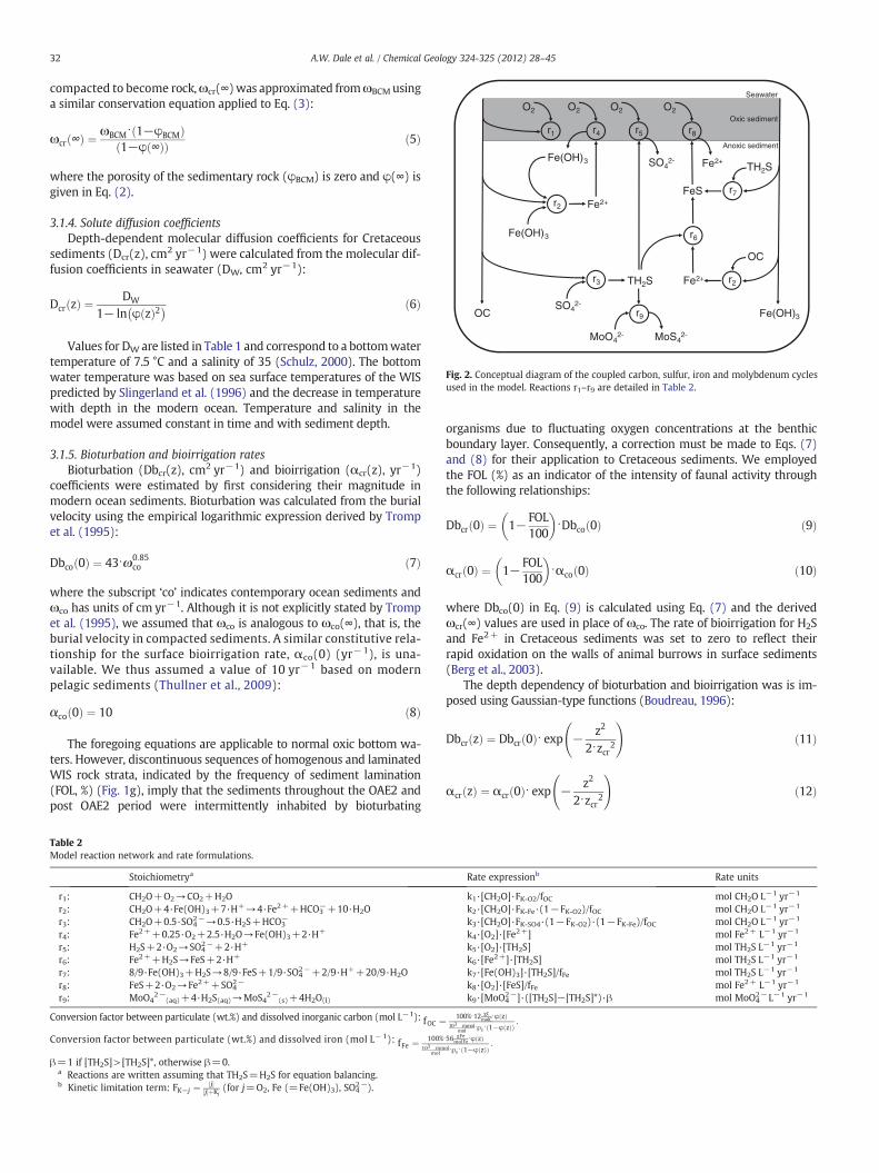
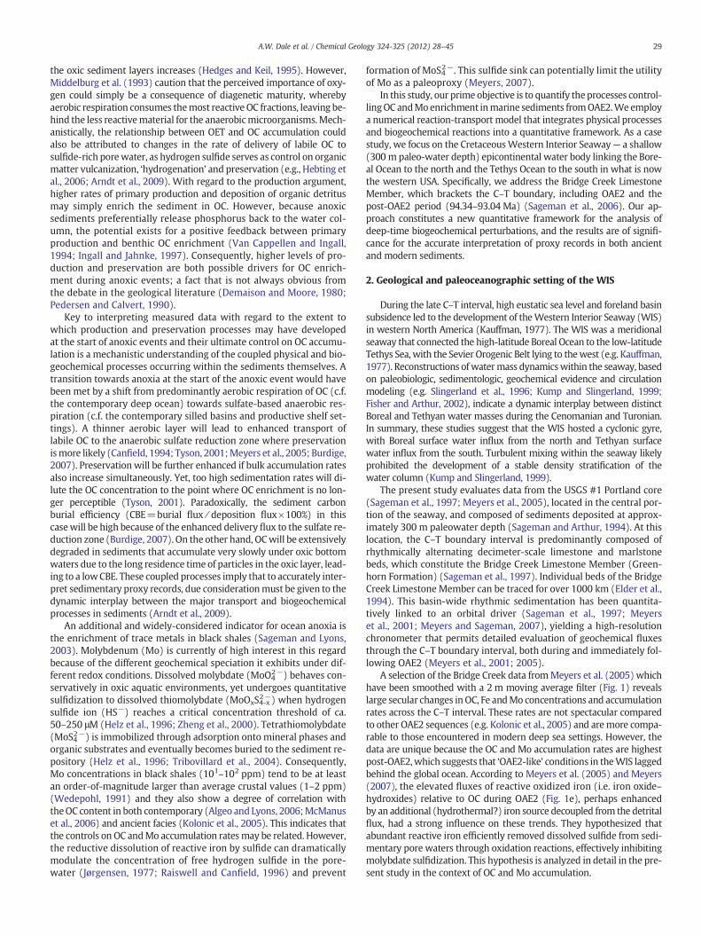
Fig. 2. Conceptual diagram of the coupled carbon, sulfur, iron and molybdenum cyclesused in the model. Reactions r1–r9 are detailed in Table 2.

32 A.W. Dale et al. / Chemical Geology 324-325 (2012) 28–45

compacted to become rock,ωcr(∞)was approximated fromωBCMusinga similar conservation equation applied to Eq. (3):

ωcr ∞ð Þ ¼ ωBCM⋅ 1−φBCMð Þ1−φ ∞ð Þð Þ ð5Þ

where the porosity of the sedimentary rock (φBCM) is zero and φ(∞) isgiven in Eq. (2).

3.1.4. Solute diffusion coefficientsDepth-dependent molecular diffusion coefficients for Cretaceous

sediments (Dcr(z), cm2 yr−1) were calculated from the molecular dif-fusion coefficients in seawater (DW, cm2 yr−1):

Dcr zð Þ ¼ DW

1− ln φ zð Þ2� � ð6Þ

Values for DW are listed in Table 1 and correspond to a bottomwatertemperature of 7.5 °C and a salinity of 35 (Schulz, 2000). The bottomwater temperature was based on sea surface temperatures of the WISpredicted by Slingerland et al. (1996) and the decrease in temperaturewith depth in the modern ocean. Temperature and salinity in themodel were assumed constant in time and with sediment depth.

3.1.5. Bioturbation and bioirrigation ratesBioturbation (Dbcr(z), cm2 yr−1) and bioirrigation (αcr(z), yr−1)

coefficients were estimated by first considering their magnitude inmodern ocean sediments. Bioturbation was calculated from the burialvelocity using the empirical logarithmic expression derived by Trompet al. (1995):

Dbco 0ð Þ ¼ 43⋅ω0:85co ð7Þ

where the subscript ‘co’ indicates contemporary ocean sediments andωco has units of cm yr−1. Although it is not explicitly stated by Trompet al. (1995), we assumed that ωco is analogous to ωco(∞), that is, theburial velocity in compacted sediments. A similar constitutive rela-tionship for the surface bioirrigation rate, αco(0) (yr−1), is una-vailable. We thus assumed a value of 10 yr−1 based on modernpelagic sediments (Thullner et al., 2009):

αco 0ð Þ ¼ 10 ð8Þ

The foregoing equations are applicable to normal oxic bottom wa-ters. However, discontinuous sequences of homogenous and laminatedWIS rock strata, indicated by the frequency of sediment lamination(FOL, %) (Fig. 1g), imply that the sediments throughout the OAE2 andpost OAE2 period were intermittently inhabited by bioturbating

Table 2Model reaction network and rate formulations.

Stoichiometrya

r1: CH2O+O2→CO2+H2Or2: CH2O+4·Fe(OH)3+7·H+→4·Fe2++HCO3

−+10·H2Or3: CH2O+0.5·SO4

2−→0.5·H2S+HCO3−

r4: Fe2++0.25·O2+2.5·H2O→Fe(OH)3+2·H+

r5: H2S+2·O2→SO42−+2·H+

r6: Fe2++H2S→FeS+2·H+

r7: 8/9·Fe(OH)3+H2S→8/9·FeS+1/9·SO42−+2/9·H++20/9·H2O

r8: FeS+2·O2→Fe2++SO42−

r9: MoO42−

(aq)+4·H2S(aq)→MoS42−(s)+4H2O(l)

Conversion factor between particulate (wt.%) and dissolved inorganic carbon (mol L−1): fOC ¼Conversion factor between particulate (wt.%) and dissolved iron (mol L−1): fFe ¼ 100%

103 mmmol

β=1 if [TH2S]>[TH2S]*, otherwise β=0.a Reactions are written assuming that TH2S=H2S for equation balancing.b Kinetic limitation term: FK−j ¼ j½ �

j½ �þKj(for j=O2, Fe (=Fe(OH)3), SO4

2−).

organisms due to fluctuating oxygen concentrations at the benthicboundary layer. Consequently, a correction must be made to Eqs. (7)and (8) for their application to Cretaceous sediments. We employedthe FOL (%) as an indicator of the intensity of faunal activity throughthe following relationships:

Dbcr 0ð Þ ¼ 1− FOL100

� �⋅Dbco 0ð Þ ð9Þ

αcr 0ð Þ ¼ 1− FOL100

� �⋅αco 0ð Þ ð10Þ

where Dbco(0) in Eq. (9) is calculated using Eq. (7) and the derivedωcr(∞) values are used in place of ωco. The rate of bioirrigation for H2Sand Fe2+ in Cretaceous sediments was set to zero to reflect theirrapid oxidation on the walls of animal burrows in surface sediments(Berg et al., 2003).

The depth dependency of bioturbation and bioirrigation was is im-posed using Gaussian-type functions (Boudreau, 1996):

Dbcr zð Þ ¼ Dbcr 0ð Þ⋅ exp − z2

2⋅zcr2

!ð11Þ

αcr zð Þ ¼ αcr 0ð Þ⋅ exp − z2

2⋅zcr2

!ð12Þ

Rate expressionb Rate units

k1·[CH2O]·FK-O2/fOC mol CH2O L−1 yr−1

k2·[CH2O]·FK-Fe·(1−FK-O2)/fOC mol CH2O L−1 yr−1

k3·[CH2O]·FK-SO4·(1−FK-O2)·(1−FK-Fe)/fOC mol CH2O L−1 yr−1

k4·[O2]·[Fe2+] mol Fe2+ L−1 yr−1

k5·[O2]·[TH2S] mol TH2S L−1 yr−1

k6·[Fe2+]·[TH2S] mol TH2S L−1 yr−1

k7·[Fe(OH)3]·[TH2S]/fFe mol TH2S L−1 yr−1

k8·[O2]·[FeS]/fFe mol Fe2+ L−1 yr−1

k9·[MoO42−]·([TH2S]−[TH2S]*)·β mol MoO4

2−L−1 yr−1

100%⋅12 gCmolC⋅φ zð Þ

103 mmolmol ⋅ρs⋅ 1−φ zð Þð Þ :

⋅56 gFemolFe⋅φ zð Þ

ol⋅ρs⋅ 1−φ zð Þð Þ:

0 20 40 60 80 100Frequency of lamination (%)

0

50

100

150

200

Bot

tom

wat

er o

xyge

n co

ncen

trat

ion

(μM

)

τ = 0.3τ = 0.05

Fig. 3. Relationship between bottom water oxygen concentration and frequency oflamination calculated with Eq. (15) using different values for the parameter τ (seetext for explanation). The gray shaded area indicates the range of frequency of lamina-tion measured in the Bridge Creek Limestone data shown in Fig. 1g.

33A.W. Dale et al. / Chemical Geology 324-325 (2012) 28–45

where zcr (cm) controls the depth of irrigation and particle mixing.Since hypoxia leads to a shallowing of habitation depth of animals(Middelburg and Levin, 2009), zcr was calculated from the mixingdepth by animals in modern sediments (zco):

zcr ¼ 1− FOL100

� �⋅zco ð13Þ

zcowas assigned a value of 5 cmbased on a global database complied byTeal et al. (2008).

3.2. Biogeochemical reaction network

The reaction network was designed to elucidate the major con-trols on OC preservation and Mo accumulation rate during the OAEand post-OAE period. For expediency, only the most important reac-tions were implemented and those suspected of having minor impor-tance were excluded. A conceptual diagram of the reaction network isshown in Fig. 2 and the kinetic rate expressions are listed in Table 2.

The primary redox reactions describe the rate of degradation of OCthrough aerobic respiration (r1), dissimilatory iron reduction (r2) andsulfate reduction (r3). The rates are first-order in OC to reflect thegeneral observation that OC availability is the rate-limiting step ofthe reaction (Berner, 1980). The rate of each pathway is determinedby the concentrations of the oxidants (i.e. O2, Fe(OH)3, SO4

2−)through kinetic limitation terms. These were formulated so that thereactions proceed sequentially as each electron acceptor becomes de-pleted with depth in the sediment. Denitrification was ignored sincenitrogen cycling is not the focus of the study and only becomes amajor pathway of carbon diagenesis in sediments underlying severelyhypoxic bottom waters (O2b20 μM) (Canfield, 1993; Bohlen et al.,2011). Carbon mineralization coupled to manganese oxide reductionwas also ignored because Mn concentrations in theWIS formation are10 times lower than iron (Sageman and Lyons, 2003) and it is gener-ally a minor pathway of carbon mineralization (Thullner et al., 2009).Finally, methanogenesis was not considered because it is inhibited bysulfate concentrations of >1 mM; conditions which do not occur inour simulations. These omissions do not seriously affect the model re-sult since >90% of benthic OC is oxidized by O2 and SO4

2− (Jørgensenand Kasten, 2006).

The secondary redox reactions are centered on Fe, S and Mo geo-chemistry (r4–r9, Table 2). The rate laws used to describe these pro-cesses employ encounter-limited, or bimolecular, kinetics. Thisapproach minimizes the number of parameters to be defined and isconsistent with the idea that the rate law should depend linearlyon the concentrations of the reactants in reactant limited-environments(Van Cappellen andWang, 1996). Ferrous iron (Fe2+) liberated by dis-similatory iron reduction can be oxidized aerobically back to particulateiron oxide (r4) or precipitated as FeS using dissolved sulfide (r6). FeS canbe oxidized aerobically (r8) or permanently buried. Dissolved sulfidecan be oxidized biologically to sulfate using oxygen (r5). In addition tooxidizing OC, Fe(OH)3 can also be used as the oxidant for chemical sul-fide oxidation (r7). Normally, this reaction is assumed to produce fer-rous iron and elemental sulfur (S0) (Van Cappellen and Wang,1996). Yet, for clarity, the net reaction is written assuming that Fe2+

production is coupled to FeS precipitation and that S0 disproportionatesto sulfide and sulfate (S0+H2O→3/4 H2S+1/4 SO4

2−). For additionalinsight into the complexities of benthic Fe and S cycles, the interestedreader is referred to Jørgensen and Kasten (2006).

The final geochemical sink for H2S is through reaction with MoO42−.

In sulfidic solution, the latter undergoes sulfidization leading to the pro-duction of tetrathiomolybdate (MoS42−):

MoOxS2−4−x aqð Þ þH2S aqð Þ⇄MoOx−1S

2−5−x aqð Þ þ H2O lð Þ ð14Þ

where 1≤x≤4.

The reaction proceeds in four steps that conserve Mo(VI), and thereaction rate decreases by an order-of-magnitude over each succes-sive step (Erickson and Helz, 2000). Consequently, mixtures of thio-molybdates can accumulate in seasonally or intermittently sulfidicporewaters. Yet, due to the long time scales of the 15 intervals mod-eled in this study (>104 yr), we assume that the equilibria can besimplified as a single step reaction between molybdate and sulfideto produce MoS42− (r9, Table 2). The bimolecular rate law prescribedfor this pathway is consistent with laboratory experiments whichshow that the sulfidization steps are first-order in the reactants(Erickson and Helz, 2000). MoS42− is particle-reactive and can be rap-idly scavenged from the pore water by metal oxyhydroxides, iron sul-fide or organic material (e.g. Vorlicek et al., 2004). Therefore, MoS42−

is modeled as a solid species on the assumption that it is immediatelysequestered by particulate phases and undergoes no further reaction.

Experiments and theory have shown that the rate of MoS42− scav-enging is rapid when HS− concentration reaches a critical pH-depen-dent threshold (Helz et al., 1996; Erickson and Helz, 2000). For a pHof 7.5 and 8.3, this threshold is equal to ca. 50 and 250 μM HS−, re-spectively, at 298 K (Helz et al., 1996). The pH of anoxic marine sed-iments is typically of the order 7.5. For this pH and the in situtemperature (280 K) and pressure (30 bar) of the WIS, HS− accountsfor around 80% of TH2S. This implies that the geochemical switch forthe above reaction should occur at in situ TH2S concentrations up-wards of ca. 65 μM. There is some field evidence to suggest thatlower sulfide thresholds (0.1 μM) are required for MoS42− scavengingonto iron minerals compared to organic material (100 μM) (Zhenget al., 2000). Since these values have yet to be confirmed by laborato-ry studies, we use the higher pH-dependent threshold sulfide concen-tration, [TH2S]*, of 65 μM whilst noting that it is likely to be somewhatsite specific. The reaction formulation only allows MoS42− formation if[TH2S] is greater or equal to [TH2S]* (r9, Table 2).

3.3. Boundary conditions

Boundary conditions at the top and bottom of the sediment columnare required to solve Eqs. (1a) and (1b). At the top, the SO4

2− concentra-tion in seawater was fixed at 10 mM to represent the Cretaceous ocean(Horita et al., 2002) and TH2Swas set to zero since theWIS was not sul-fidic (Table 1). Proposed fluctuations in SO4

2− concentration throughout

34 A.W. Dale et al. / Chemical Geology 324-325 (2012) 28–45

the Cretaceous of between 2 and 12 mM (Wortmann and Chernyavsky,2007; Adams et al., 2010) are not likely to have an important impact onthe model results since methanogenesis will only become important ifSO4

2− falls to b1 mM. Boundary conditions for the other species are de-scribed separately below. At the bottom of the simulated sediment col-umn (150 cm depth), all species are prescribed with zero-gradient(Neumann) boundary conditions.

3.3.1. Bottom water oxygen concentrationOxygen concentrations at the benthic boundary layer in the WIS,

[O2]cr(0), were estimated using a method borrowed from a study onthe hypoxic St. Lawrence River estuary by Katsev et al. (2007). Theseworkers scanned intact sediment cores from siteswith different bottomwater oxygen concentrations using computerized axial tomography inorder to observe the effect of decreasing oxygen on bioturbation andsediment structure. They derived a non-linear empirical relationshipbetween bioturbation and oxygen concentrations which we use as thebasis for our model. Using this relationship and the equality betweenDbcr(0) and FOL in Eq. (9), [O2]cr(0) can be calculated as follows:

O2½ �cr 0ð Þ ¼ O2½ ��−1τ⋅ ln FOL

100−FOL

� �ð15Þ

where [O2]* is the threshold oxygen concentration due to hypoxiawhich leads to large changes in faunal community structure. Mechanis-tically, [O2]* defines the oxygen concentration at which Dbcr(0) falls tohalf the value of Dbco(0) due to severe hypoxia (Katsev et al., 2007). Itis assigned a value of 62 μM based on work by Diaz and Rosenberg(1995). The time-invariant coefficient, τ, controls the steepness in de-cline of [O2]cr(0) with increasing FOL. This parameter was assigned avalue of 0.3 by Katsev et al. (2007).

The relationship between [O2]cr(0) and FOL for two values of τ isshown in Fig. 3, where the shaded band indicates the region corre-sponding to the FOL from the WIS. The parameter τ controls thesteepness of the curve whereas [O2]* determines its vertical displace-ment. The range in [O2]cr(0) is small (61–70 μmol L−1) for the value

Sediment accumulation rate (g cm-2yr-1)0.0001 0.001 0.01 0.1 1 10

0.1

1

10

100

Car

bon

buria

l effi

cien

cy (

%)

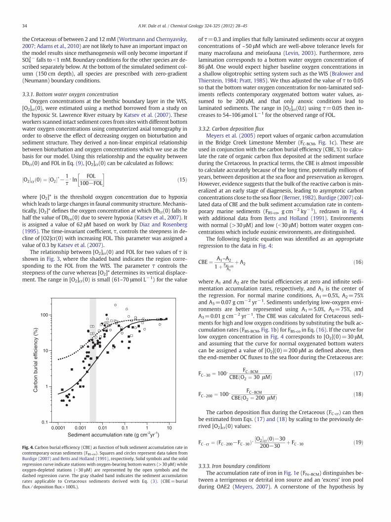
Fig. 4. Carbon burial efficiency (CBE) as function of bulk sediment accumulation rate incontemporary ocean sediments (FBS-co). Squares and circles represent data taken fromBurdige (2007) and Betts and Holland (1991), respectively. Solid symbols and the solidregression curve indicate stations with oxygen-bearing bottom waters (>30 μM) whileoxygen-depleted stations (b30 μM) are represented by the open symbols and thedashed regression curve. The gray shaded band indicates the sediment accumulationrates applicable to Cretaceous sediments derived with Eq. (3). (CBE=burialflux∕deposition flux×100%.).

of τ=0.3 and implies that fully laminated sediments occur at oxygenconcentrations of ~50 μM which are well-above tolerance levels formany macrofauna and meiofauna (Levin, 2003). Furthermore, zerolamination corresponds to a bottom water oxygen concentration of86 μM. One would expect higher baseline oxygen concentrations ina shallow oligotrophic setting system such as the WIS (Bralower andThierstein, 1984; Pratt, 1985). We thus adjusted the value of τ to 0.05so that the bottom water oxygen concentration for non-laminated sed-iments reflects contemporary oxygenated bottom water values, as-sumed to be 200 μM, and that only anoxic conditions lead tolaminated sediments. The range in [O2]cr(0,t) using τ=0.05 then in-creases to 54–106 μmol L−1 for the observed range of FOL.

3.3.2. Carbon deposition fluxMeyers et al. (2005) report values of organic carbon accumulation

in the Bridge Creek Limestone Member (FC-BCM, Fig. 1c). These areused in conjunction with the carbon burial efficiency (CBE, %) to calcu-late the rate of organic carbon flux deposited at the sediment surfaceduring the Cretaceous. In practical terms, the CBE is almost impossibleto calculate accurately because of the long time, potentially millions ofyears, between deposition at the sea floor and preservation as kerogen.However, evidence suggests that the bulk of the reactive carbon is min-eralized at an early stage of diagenesis, leading to asymptotic carbonconcentrations close to the sea floor (Berner, 1982). Burdige (2007) col-lated data of CBE and the bulk sediment accumulation rate in contem-porary marine sediments (FBS-co, g cm−2 ky−1), redrawn in Fig. 4with additional data from Betts and Holland (1991). Environmentswith normal (>30 μM) and low (b30 μM) bottom water oxygen con-centrations which include euxinic environments, are distinguished.

The following logistic equation was identified as an appropriateregression to the data in Fig. 4:

CBE ¼ A1–A2

1þ FBS�coA3

þ A2 ð16Þ

where A1 and A2 are the burial efficiencies at zero and infinite sedi-mentation accumulation rates, respectively, and A3 is the center ofthe regression. For normal marine conditions, A1=0.5%, A2=75%and A3=0.07 g cm−2 yr−1. Sediments underlying low-oxygen envi-ronments are better represented using A1=5.0%, A2=75%, andA3=0.01 g cm−2 yr−1. The CBE was calculated for Cretaceous sedi-ments for high and low oxygen conditions by substituting the bulk ac-cumulation rates (FBS-BCM, Fig. 1b) for FBS-co in Eq. (16). If the curve forlow oxygen concentration in Fig. 4 corresponds to [O2](0)=30 μM,and assuming that the curve for normal oxygenated bottom waterscan be assigned a value of [O2](0)=200 μM as defined above, thenthe end-member OC fluxes to the sea floor during the Cretaceous are:

FC�30 ¼ 100⋅ FC�BCM

CBE O2 ¼ 30 μMð Þ ð17Þ

FC�200 ¼ 100⋅ FC�BCM

CBE O2 ¼ 200 μMð Þ ð18Þ

The carbon deposition flux during the Cretaceous (FC-cr) can thenbe estimated from Eqs. (17) and (18) by scaling to the previously de-rived [O2]cr(0) values:

FC�cr ¼ FC�200−FC�30ð Þ⋅ O2½ �cr 0ð Þ−30200−30

þ FC�30 ð19Þ

3.3.3. Iron boundary conditionsThe accumulation rate of iron in Fig. 1e (FFe-BCM) distinguishes be-

tween a terrigenous or detrital iron source and an ‘excess’ iron poolduring OAE2 (Meyers, 2007). A cornerstone of the hypothesis by

k6

k5

k4

k7

0 2 4 6 8 10 12 14 16

log10 M-1 yr-1

k8

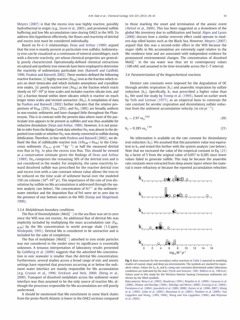
Fig. 5. Rate constants for the secondary redox reactions in Table 2 reported in modelingstudies of coastal, slope and deep sea environments. The symbols are stacked for equiv-alent values. Values for k4, k5 and k7 using rate constants determined under laboratoryconditions are indicated by the stars (Pyzik and Sommer, 1981; Millero et al., 1987a,b).Values used in this study for the Western Interior Seaway Cretaceous sediments areshown by the filled symbols.Data sources: Berg et al. (2003); Boudreau (1991); Brigolin et al. (2009); Canavan et al.(2006); Dhakar and Burdige (1996); Eldridge and Morse (2000); Fossing et al. (2004);Furukawa et al. (2004); Jourabchi et al. (2005, 2008); Katsev et al. (2006, 2007); Königet al. (1999); Linke et al. (2005); Meysman et al. (2003); Thullner et al. (2009); VanCappellen and Wang, (1995, 1996); Wang and Van Cappellen (1996); and Wijsmanet al. (2002).

35A.W. Dale et al. / Chemical Geology 324-325 (2012) 28–45

Meyers (2007) is that the excess iron was highly reactive, possiblyhydrothermal in origin (e.g., Snow et al., 2005), and promoted sulfidebuffering and low Mo accumulation rates during OAE2 in the WIS. Toaddress this hypothesis effectively, the fluxes and reactivity of detritaland excess iron must be considered individually.

Based on Fe–C–S relationships, Dean and Arthur (1989) arguedthat the iron is mainly present as particulate iron sulfides. Sedimenta-ry iron can be visualized as a continuum of mineral assemblages, eachwith a discrete reactivity, yet whose chemical properties are general-ly poorly characterized. Operationally-defined chemical extractionson natural and synthetic ironminerals have been employed to determinethe reactivity of sedimentary particulate iron (Raiswell and Canfield,1996; Poulton and Raiswell, 2002). These workers defined the followingreactive fractions; (i) highly reactive (FeHR) iron as the fractionwhich re-acts on short timescales and which includes amorphous and crystallineiron oxides, (ii) poorly reactive iron (FePR) as the fraction which reactsslowly on 105–106 yr time scales and includes reactive silicate iron, and(iii) a fraction bound within sheet silicates which is reactive on muchlonger times scales and termed unreactive (FeU). A compilation of databy Poulton and Raiswell (2002) further indicates that the relative pro-portions of FeHR (25%), FePR (25%), and FeU (50%) are broadly uniformin non-euxinic sediments and have changed little throughout the Phan-erozoic. This is in contrast with the present data where most of the par-ticulate iron appears to be present as sulfides and was thus available forreductive dissolution (Dean and Arthur, 1989). However, it is not possi-ble to infer from the Bridge Creek datawhether FeUwas absent in the de-posited iron oxide orwhether FeUwas slowly converted to sulfide duringlithification. Therefore, in line with Poulton and Raiswell (2002), we de-fined the flux of sulfidizable reactive iron (≡FeHR+FePR) to the Creta-ceous sediments (FFe-cr, g cm−2 ky−1) as half the measured detritaliron flux in Fig. 1e plus the excess iron flux. This should be viewedas a conservative estimate given the findings of Dean and Arthur(1989). FeU comprises the remaining 50% of the detrital iron and isnot considered in the model. For simplicity, the same reactivity to-ward dissolved sulfide was prescribed for the reactive detrital ironand excess iron with a rate constant whose value allows the iron tobe reduced on the time scale of sediment burial over the modeled150 cm column (104–105 yr). The importance of the rate of iron dis-solution by sulfide onMo accumulation is addressed through the sys-tem analysis (see below). The concentration of Fe2+ at the sediment–water interface and the deposition flux of FeS were set to zero due tothe presence of oxic bottom waters in the WIS (Kump and Slingerland,1999).

3.3.4. Molybdenum boundary conditionsThe flux of thiomolybdate (MoS42−) to the sea floor was set to zero

since the WIS was not euxinic. An additional flux of detrital Mo wasimplicitly included by multiplying the mass accumulation rate (FBS-BCM) by the Mo concentration in world average shale (1.5 ppm;Wedepohl, 1991). Detrital Mo is considered to be unreactive and isincluded for the sake of completion.

The flux of molybdate (MoO42−) adsorbed to iron oxide particles

was not considered in the model since its significance is essentiallyunknown. A tenuous interpretation of laboratory results presentedby Goldberg et al. (2009) suggests that the adsorbed Mo concentra-tion in oxic seawater is smaller than the detrital Mo concentration.Furthermore, several studies across a broad range of oxic and anoxicsettings have reported that processes occurring at or below the sedi-ment water interface are mainly responsible for Mo accumulation(e.g. Crusius et al., 1996; Erickson and Helz, 2000; Zheng et al.,2000). Transport of dissolved molybdate across the sediment–waterinterface was thus assumed to be the only source of reactive Mo, al-though the processes responsible for Mo accumulation are still poorlyunderstood.

It should be mentioned that Mo enrichment in some black shalesfrom the proto-North Atlantic is lower in the OAE2 sections compared

to those marking the onset and termination of the anoxic event(Hetzel et al., 2009). This has been suggested as a drawdown of theglobal Mo inventory due to sulfidization and burial. Algeo and Lyons(2006) discuss how a similar reservoir effect could operate in mod-ern-day silled basins such as the Black Sea. However, Meyers (2007)argued that this was a second-order effect in the WIS because themajor shifts in Mo accumulation are extremely rapid relative to theMo residence time and are associated with independent evidence forpronounced environmental changes. The concentration of dissolvedMoO4

2− in the sea water was thus set to contemporary values(100 nM) and assumed to be time-invariable across the C–T interval.

3.4. Parameterization of the biogeochemical reactions

Distinct rate constants were imposed for the degradation of OCthrough aerobic respiration (k1) and anaerobic respiration by sulfatereduction (k3). Specifically, k1 was prescribed a higher value thank3. We used the study by Tromp et al. (1995), based on earlier workby Toth and Lerman (1977), as an empirical basis to constrain therate constant for aerobic respiration and dissimilatory sulfate reduc-tion from the sediment accumulation velocity (in cm yr−1):

k1 ¼ 2:97⋅ωcr0:62 ð20Þ

k3 ¼ 0:285⋅ωcr1:94 ð21Þ

No information is available on the rate constant for dissimilatoryiron reduction (k2). We assumed that this parameter value was equiva-lent to k3 and tested this further with the system analysis (see below).Note that we increased the value of the empirical constant in Eq. (21)by a factor of 5 from the original value of 0.057 to 0.285 since lowervalues failed to generate sulfide. This may be because the anaerobicrate constants were extracted from deep anoxic layers where themate-rial is more refractory or because the reported accumulation velocities

36 A.W. Dale et al. / Chemical Geology 324-325 (2012) 28–45

correspond to surface sediments where sediment burial velocities arehigher. Nonetheless, the resulting k3 values using Eq. (21) are withinthe scatter of the data presented by Tromp et al. (1995).

No similar constitutive relationships exist for the rate constants ofthe secondary redox reactions (r4–r8, Table 2). We attempted to over-come this problem by analyzing previous modeling studies from arange of oxic and anoxic basins from the continental shelf to the deepsea where bimolecular rate constants have been reported (Fig. 5). Therange of values overmany orders-of-magnitude is quite striking. For ex-ample, the rate constant values for aerobic sulfide oxidation (k5) ex-tend over 10 orders-of-magnitude. The lower end estimates of1.6·105 M−1 yr−1 (Van Cappellen and Wang, 1995; Wang and VanCappellen, 1996) were based on experiments by Millero et al.(1987a). At the upper end of the scale, Boudreau (1991) constrainedk5 to 1.0·1015 M−1 yr−1 using field data from Aarhus Bay sedi-ments. This anomaly is easily explained by the role of sulfide-oxidizingmicroorganisms. The laboratory experiments were performed underabiological conditions whereas sulfide-oxidizing bacteria are presentin abundance at the site investigated byBoudreau (1991) and efficientlycatalyze the reaction between sulfide and oxygen.

Rate constants for secondary redox reactions are generally regardedasfitting parameters inmodels and thus integrate the effect ofmany en-vironmental variables. These include (i) the role of ionic strength andpH, (ii) thermodynamic constraints on reactions imposed though thepore water chemistry, (iii) geochemical catalysts or inhibitors, and(iv) microbial community structure. The spread of reported values inFig. 5 likely reflects a change in the relative importance of these vari-ables among the contrasting environments. Nonetheless, more thanhalf of the studies listed report that the rate constants were ‘con-strained’ or ‘fitted’ using site-specific data, yet contain little or no rele-vant model-data comparison to evaluate the goodness-of-fit. It shouldbe remembered that sediment reaction-transport models are coupledthrough the chemical species and that ‘fitted’may refer to a specific as-pect or output of themodel. Thismeans that a parameter value could besourced fromelsewhere in the literature, yet still be reported as ‘fitted’ ifthe overall model output is satisfactory. Rate constants k4–k8 for theWIS were estimated only from those studies that provide some indica-tion of the validity of the parameterizations, i.e. concentration or ratedata, and were further assumed to be time-invariant.

The considerable uncertainty in the unknown rate constants andthe parameters used to hindcast the boundary conditions, is not amajor cause for concern. The highly coupled nature of the reactionnetwork places constraints on the number of possible permutationsof the entire set of model parameters when tested against field data(Van Cappellen and Wang, 1996). That is, large errors in a single pa-rameters or forcing functions will become obvious in one or more ofthe modeled variables. Simultaneous reconstruction of OC, Mo andFe concentrations and accumulation rates is a firm indication thatthe parameterization is satisfactory. The uncertainty if further quanti-fied using the system analysis described below.

3.5. Numerical solution

The set of coupled partial differential equations for solutes andsolids was transformed using the method of lines (Boudreau, 1996).The resulting set of ordinary differential equations was solved usingthe NDSolve algorithm in MATHEMATICA over a grid spacing increas-ing from sub-mm at the top of the core to sub-cm at the bottom witha total of 100 depth intervals. The model typically requires ca. 120 s tocomplete a single simulation.

3.6. System analysis

The reaction network is limited to 9 reactions and is thus relative-ly small compared to other diagenetic models (e.g. Van Cappellenand Wang, 1996). Yet, it is nonetheless a highly interconnected

biogeochemical system. One is thus confronted with a large numberof potential couplings between parameter values and boundary con-ditions that control the Mo and OC accumulation rate. A piecewiseanalysis of the model, that is, changing single parameter valuesone-by-one and observing the change in model output, is not an op-timal means of accurately determining the major controls on specificprocesses since it cannot identify important couplings betweenparameters.

To disentangle the interconnectivity in the model, we carried out asystem analysis based on a two-level factorial design. Factorial analy-sis is a statistical methodology (Box et al., 1978) that determines theresponse of a pre-defined system output (e.g. a reaction rate or con-centration) to a change in n model ‘factors’ (e.g. parameters orboundary conditions). Each factor is assigned a high and low level,such that for n factors there are a total of 2n system responses. The ‘ef-fect’ of all possible factor permutations is calculated from the re-sponses using a simple algorithm. The effects can then be illustratedon a normal probability plot to visualize the factor or interactionsthereof that have the largest impact on the system response (Boxet al., 1978). An example of an application of factorial analysis to ma-rine sediment dynamics is given by Dale et al. (2006, 2011).

In this study, three model responses have been identified: Mo andOC accumulation rate (or the burial rate at the lower model boundaryof 150 cm) and the corresponding CBE. Two factorial analyses wereperformed using the factors suspected to have the largest effect onthese responses. The first set of factors tested were those associatedwith transport and boundary conditions, that is, the environmentalparameters (FC-cr, FFe-cr, ωcr(∞), Dbcr(0), αcr(0), zcr, [O2]cr(0)). The 7environmental factors require (27=) 128 model simulations to fullytest the complete array of factor combinations. The second set focuseson the reaction-specific parameters which are the biogeochemical rateconstants (k1 to k8), requiring a further (28=) 256 simulations. The fac-tors which directly control Mo accumulation (FMoS4-cr, [MoO4

2−]cr(0),k9 and [TH2S]*) were not included since the interest is on the peripheralmechanisms which are conducive to authigenic Mo accumulation inCretaceous sediments.

To elucidate the major controlling factors onMo and OC burial andCBE across the C–T interval, the high and low factor levels were deter-mined from their mean values derived for the OAE2 and post-OAE2period. The values for the rate constants k4 to k8 were fixed in themodel and not derived from the data. Their prescribed values in thefactorial analysis were determined by varying the baseline values inTable 1 by ±50%. Although this is much lower than the reported pa-rameter values (Fig. 5), it is the same relative change calculated forthe other derived parameters (see Table 3, Results). It is importantto remember that the system analysis results may not be universallyapplicable and are only valid for the specific ranges over which thefactors were varied.

4. Results

4.1. Critical examination of model forcings and comparison with modernpelagic sediments

The parameters and boundary conditions derived in Section 3 ap-plicable to the unconsolidated Cretaceous sediments are shown inFig. 6. Averaged values for the OAE2 and post-OAE2 periods are sum-marized in Table 3 and compared to those from contemporary marinesettings where possible.

The derivedmean sediment burial velocity,ωcr(∞), varies over time,ranging from 3.2 to 4.4 cm ky−1 (Fig. 6a, Table 3). These are similar tothose encountered in the modern deep ocean but around 3 timeslower than the OAE2 sequences of Tarfaya Basin in the proto-North At-lantic (Kolonic et al., 2005). Consequently, the bioturbation coefficients(Dbcr(0), Fig. 6b) are also similar to deep sea values since Dbcr(0) is de-rived from ωcr(∞). Bioirrigation coefficients, αcr(0), of 4 to 9 yr−1

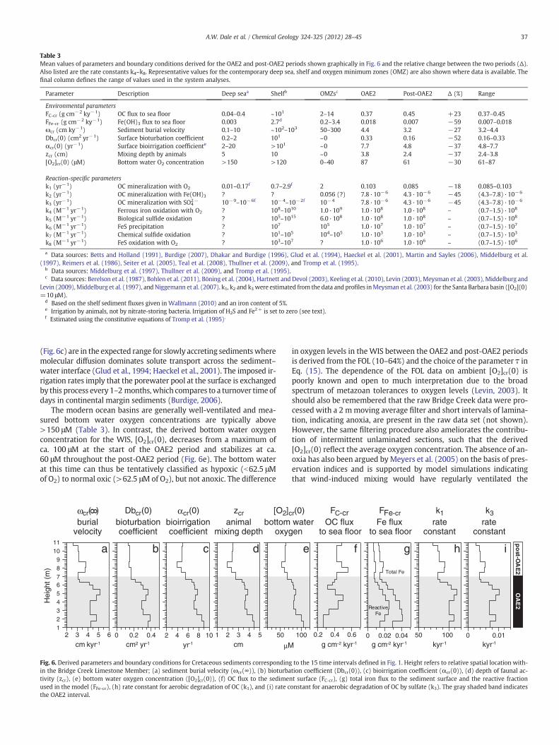
Table 3Mean values of parameters and boundary conditions derived for the OAE2 and post-OAE2 periods shown graphically in Fig. 6 and the relative change between the two periods (Δ).Also listed are the rate constants k4–k8. Representative values for the contemporary deep sea, shelf and oxygen minimum zones (OMZ) are also shown where data is available. Thefinal column defines the range of values used in the system analyses.

Parameter Description Deep seaa Shelfb OMZsc OAE2 Post-OAE2 Δ (%) Range

Environmental parametersFC-cr (g cm−2 ky−1) OC flux to sea floor 0.04–0.4 ~101 2–14 0.37 0.45 +23 0.37–0.45FFe-cr (g cm−2 ky−1) Fe(OH)3 flux to sea floor 0.003 2.7d 0.2–3.4 0.018 0.007 −59 0.007–0.018ωcr (cm ky−1) Sediment burial velocity 0.1–10 ~102–103 50–300 4.4 3.2 −27 3.2–4.4Dbcr(0) (cm2 yr−1) Surface bioturbation coefficient 0.2–2 101 ~0 0.33 0.16 −52 0.16–0.33αcr(0) (yr−1) Surface bioirrigation coefficiente 2–20 >101 ~0 7.7 4.8 −37 4.8–7.7zcr (cm) Mixing depth by animals 5 10 ~0 3.8 2.4 −37 2.4–3.8[O2]cr(0) (μM) Bottom water O2 concentration >150 >120 0–40 87 61 −30 61–87

Reaction-specific parametersk1 (yr−1) OC mineralization with O2 0.01–0.17f 0.7–2.9f 2 0.103 0.085 −18 0.085–0.103k2 (yr−1) OC mineralization with Fe(OH)3 ? ? 0.056 (?) 7.8·10−6 4.3·10−6 −45 (4.3–7.8)·10−6

k3 (yr−1) OC mineralization with SO42− 10−9–10−6f 10−4–10−2f 10−4 7.8·10−6 4.3·10−6 −45 (4.3–7.8)·10−6

k4 (M−1 yr−1) Ferrous iron oxidation with O2 ? 108–1010 1.0·109 1.0·108 1.0·108 – (0.7–1.5)·108

k5 (M−1 yr−1) Biological sulfide oxidation ? 105–1015 6.0·108 1.0·108 1.0·108 – (0.7–1.5)·108

k6 (M−1 yr−1) FeS precipitation ? 107 105 1.0·107 1.0·107 – (0.7–1.5)·107

k7 (M−1 yr−1) Chemical sulfide oxidation ? 101–105 104–105 1.0·103 1.0·103 – (0.7–1.5)·103

k8 (M−1 yr−1) FeS oxidation with O2 ? 103–107 ? 1.0·106 1.0·106 – (0.7–1.5)·106

a Data sources: Betts and Holland (1991), Burdige (2007), Dhakar and Burdige (1996), Glud et al. (1994), Haeckel et al. (2001), Martin and Sayles (2006), Middelburg et al.(1997), Reimers et al. (1986), Seiter et al. (2005), Teal et al. (2008), Thullner et al. (2009), and Tromp et al. (1995).

b Data sources: Middelburg et al. (1997), Thullner et al. (2009), and Tromp et al. (1995).c Data sources: Berelson et al. (1987), Bohlen et al. (2011), Böning et al. (2004), Hartnett and Devol (2003), Keeling et al. (2010), Levin (2003), Meysman et al. (2003), Middelburg and

Levin (2009),Middelburg et al. (1997), and Niggemann et al. (2007). k1, k2 and k3were estimated from the data and profiles inMeysman et al. (2003) for the Santa Barbara basin ([O2](0)=10 μM).

d Based on the shelf sediment fluxes given in Wallmann (2010) and an iron content of 5%.e Irrigation by animals, not by nitrate-storing bacteria. Irrigation of H2S and Fe2+ is set to zero (see text).f Estimated using the constitutive equations of Tromp et al. (1995).

37A.W. Dale et al. / Chemical Geology 324-325 (2012) 28–45

(Fig. 6c) are in the expected range for slowly accreting sedimentswheremolecular diffusion dominates solute transport across the sediment–water interface (Glud et al., 1994; Haeckel et al., 2001). The imposed ir-rigation rates imply that the porewater pool at the surface is exchangedby this process every 1–2 months,which compares to a turnover time ofdays in continental margin sediments (Burdige, 2006).

The modern ocean basins are generally well-ventilated and mea-sured bottom water oxygen concentrations are typically above>150 μM (Table 3). In contrast, the derived bottom water oxygenconcentration for the WIS, [O2]cr(0), decreases from a maximum ofca. 100 μM at the start of the OAE2 period and stabilizes at ca.60 μM throughout the post-OAE2 period (Fig. 6e). The bottom waterat this time can thus be tentatively classified as hypoxic (b62.5 μMof O2) to normal oxic (>62.5 μM of O2), but not anoxic. The difference

123456789

1011

Hei

ght (

m)

2 3 4 5 6 0 0.2 0.4 2 4 6 8 10 1 2 3 4 5 50

a b c d

Fig. 6. Derived parameters and boundary conditions for Cretaceous sediments correspondingin the Bridge Creek Limestone Member; (a) sediment burial velocity (ωcr(∞)), (b) bioturbativity (zcr), (e) bottom water oxygen concentration ([O2]cr(0)), (f) OC flux to the sedimenused in the model (FFe-cr), (h) rate constant for aerobic degradation of OC (k1), and (i) rate cthe OAE2 interval.

in oxygen levels in theWIS between the OAE2 and post-OAE2 periodsis derived from the FOL (10–64%) and the choice of the parameter τ inEq. (15). The dependence of the FOL data on ambient [O2]cr(0) ispoorly known and open to much interpretation due to the broadspectrum of metazoan tolerances to oxygen levels (Levin, 2003). Itshould also be remembered that the raw Bridge Creek data were pro-cessed with a 2 mmoving average filter and short intervals of lamina-tion, indicating anoxia, are present in the raw data set (not shown).However, the same filtering procedure also ameliorates the contribu-tion of intermittent unlaminated sections, such that the derived[O2]cr(0) reflect the average oxygen concentration. The absence of an-oxia has also been argued by Meyers et al. (2005) on the basis of pres-ervation indices and is supported by model simulations indicatingthat wind-induced mixing would have regularly ventilated the

100 50 1000.2 0.4 0.6 0 0.02 0.04 0 0.01

Total Fe

ReactiveFe

OA

E2

po

st-OA

E2

e f g h i

to the 15 time intervals defined in Fig. 1. Height refers to relative spatial location with-tion coefficient (Dbcr(0)), (c) bioirrigation coefficient (αcr(0)), (d) depth of faunal ac-t surface (FC-cr), (g) total iron flux to the sediment surface and the reactive fractiononstant for anaerobic degradation of OC by sulfate (k3). The gray shaded band indicates

38 A.W. Dale et al. / Chemical Geology 324-325 (2012) 28–45

shallow bottom waters of the WIS (Kump and Slingerland, 1999). Onbalance, the presence of a deep hypoxic water layer across the C–T in-terval seems more reasonable than anoxic or sulfidic bottom waters.

The flux of OC to the sediment–water interface (FC-Cr, Fig. 6f), rangesfrom 0.37 to 0.45 g cm−2 ky−1. This is comparable to those on thelower continental slope and abyss in the modern ocean, but at least afactor of 10 lower than sediments on the shelf and from oxygen mini-mum zones (Table 3). This is a further indication that the WIS musthave been significantly oligotrophic compared to the modern ocean ofcomparable water depths (300 m) where one would expect to find OCfluxes of ca. 1–5 g cm−2 ky−1 (Burdige, 2007; Thullner et al., 2009).Our approach further predicts that the post-OAE2 sediments receiveda 20% higher flux of OC relative to those in the OAE2 period. Yet, thedata show that carbonate accumulation rates were lower post-OAE2(Fig. 1d), which led Meyers et al. (2005) to argue that paleoproduction,and thus FC-Cr, were also lower during this interval. We return to thisdiscrepancy in more detail in the Discussion.

The imposed reactive iron fluxes are compared with the total ironflux in Fig. 6g which includes the unreactive iron fraction. There isvery little data in the literature for comparison of these fluxes. Model-constrained reactive iron fluxes for the deep MANOP sites (Dhakarand Burdige, 1996) and mass balances for Pacific pelagic clays (Glasby,1991) are in the region of 0.003 g cm−2 ky−1. These are up to a factorof 10 lower than those measured in the Bridge Creek data. On thisbasis, we infer that the WIS sediments received a disproportionatelylarge flux of reactive iron compared to carbon with respect to othermodern deep sea (Table 3) or ancient (e.g. Hetzel et al., 2009) ocean an-alogs. For comparison, iron fluxes in contemporary shelf sediments are2–3 orders-of-magnitude higher (Table 3) since most terrigenous par-ticulate material is trapped and buried there (Wallmann, 2010).

The rate constant for aerobic OC mineralization, k1, ranges from 74to 113 ky−1, which is ca. 4–5 orders-of-magnitude larger than therate constant for anaerobic mineralization by sulfate reduction (k3)which ranges from 5.5·10−4 to 2.1·10−3 yr−1 (Fig. 6h,i). There is noscientific consensus on a theory that clearly explains these differencesand themajor theories proposed have been detailed in the Introduction.Nonetheless, the constitutive equations used by Tromp et al. (1995) toderive the rate constants are empirically based and have been shownto provide a good estimate of carbon burial efficiencies in contemporarymarine sediments (Meile andVan Cappellen, 2005). Even so, the assign-ment of a single rate constant value at any given time conflicts with theobservation that OC degrades at different rates over a wide spectrum oftemporal and spatial scales (Westrich and Berner, 1984; Middelburg,1989). For example, the inclusion of 2 or 3 different OC pools are often

12

3

4

5

6

7

8

9

10

11

Hei

ght(

m)

a b c d

0 0.05 0 0.01 0.02 0.03 0 10 20 30 0 1 2

±0.005

±0.014 ±6

Fig. 7. Comparison between measured (circles, from Fig. 1) and modeled (thin lines) data fro(Fe(OH)3+FeS) (FFe-BCM), (c) Mo (FMo-BCM), and concentrations of (d) OC, (e) total iron (Fe(and accumulation rates are calculated at the bottom of the simulated core. (b) and (e) onlyFig. 1e (see Section 3.3.3). The dashed lines in (c) and (f) indicate detrital Mo and the graydication of the error in the model. These are calculated from the system analysis (Fig. 9), a

required to adequately simulate anaerobic OCmineralization by sulfatereduction (Dale et al., 2009). Yet, we argue that the need for additionalOC pools in model simulations is less important for oligotrophic envi-ronments with low sediment burial velocities compared to eutrophicsettings with high sediment burial velocities. This is because muchmore of the reactive carbon will be mineralized by aerobic processesin the water column and the uppermost surface layers in oligotrophicsystems, leading to decreased burial rates of reactive fractions(Middelburg, 1989). In other words, the suitability of the Trompet al. (1995) equations in describing a single bulk OC pool undergo-ing either aerobic or anaerobic decomposition may increase with de-creasing sediment burial velocity. Given that the sediments of the WISaccumulated at rates similar to those in the contemporary deep sea,the use of a single rate constant in the model seems to be defensible.

4.2. Geochemical characteristics of Cretaceous sediments

The results of the 15 steady state model simulations are shown inFig. 7 (thick lines), which compares modeled and measured accumu-lation rates and concentrations of OC, Fe and Mo. Model-predictedCBEs are also presented. OAE2 is characterized by relatively low OCand Mo accumulation rates and high Fe accumulation, whereas OCand Mo accumulation rates are relatively high and Fe accumulationrates are low following this global event. To put these data in perspec-tive, the Mo accumulation rates of ca. 7–14 μg cm−2 kyr−1 (Fig. 7c)are much lower than the range of 50–1500 μg cm−2 kyr−1 reportedfor modern sediments (Zheng et al., 2000; McManus et al., 2006;Morford et al., 2009; Scholz et al., 2011). Overall, the model showsgood agreement with the observations and is able to reproduce themajor trends in the data. This provides some confidence that the reac-tion network and parameterizations are satisfactory. A series of causalmechanisms explaining these trends has been proposed (Meyerset al., 2005; Meyers, 2007) which we discuss later in conjunctionwith the results from the system analysis. Beforehand, we explorehow the sediment porewater and solid phase concentration profilesmay have evolved in the unconsolidated sediments.

The geochemical profiles of solids and solutes in the unconsolidatedCretaceous sediments shown in Fig. 8 are generated by running themodel using themean parameter values for the OAE2 and post-OAE2 pe-riod (Table 3). The model predicts a ca. 20 mm penetration depth of O2

into the sediment during OAE2. Thus, despite contemporaneous globalanoxia, theWIS sediments retain a relatively thick upper oxic layer sim-ilar to the modern deep sea (Reimers et al., 1986). Moreover, aerobicrespiration accounts for 99% of total OC mineralization over the upper

e f

3 4 0 1 2 0 5 10 15 20 0 5 10 15

g

OA

E2

po

st-OA

E2

±0.7 ±0.27 ±3.6 ±4.5

m Bridge Creek Limestone Member. Accumulation rate of (a) OC (FC-BCM), (b) total ironOH)3+FeS), (f) Mo, and (g) carbon burial efficiency (CBE). The modeled concentrationsshow the simulation of the reactive iron pool with that calculated from the raw data inshaded band shows the OAE2 interval. The thick lines denote the uncertainty — an in-nd correspond to the largest observed effect (boxed numbers in each panel, see text).

150

100

50

0

3

2

1

0

ihgf

edca b

0 50 100 1500 100 2009 10 110 50 100 0 1 2

150

100

50

00 10 5 10 150 1 2 3 4 50 1 2 3 4 5

Fig. 8.Modeled steady state concentration–depth profiles representative of the unconsolidated Cretaceous sediments of OAE2 (solid circles) and post-OAE2 (open circles). Note thedifferent depth scale in the oxygen profile.

39A.W. Dale et al. / Chemical Geology 324-325 (2012) 28–45

150 cm (Table 4). Iron and sulfate reduction account for b1% and sulfateconcentration barely decreases over the model sediment column. Thesame tendencies have been quantified in contemporary deep sea sedi-ments (Jahnke et al., 1982; Dhakar and Burdige, 1996; Haeckel et al.,2001), which reiterates the oligotrophic nature of the WIS over the C–T interval. Particulate (reactive) iron decreases from ca. 3 wt.% at thesurface to ca. 1 wt.% at the base of the simulated sediment core due toreductive dissolution (Fig. 8g). This implies that sulfate reduction andrelease of sulfide to the porewater would only become significant at agreater depth than modeled here. These concentrations agree with ob-servations in the Peru Basin (König et al., 1997) but are lower thanPacific red clays that have iron contents in excess of 5 wt.% (Glasby,1991). The presence of reactive iron severely inhibits the rate of sulfideproduction by dissimilatory sulfate reduction and particulate Mo con-centrations remain at the detrital background level of 1.5 ppm (Fig. 8h).

The sediments below the oxic layer are highly ferruginous withFe2+ concentrations reaching 1 mM at 150 cm. These high levels con-trast with reports of low or undetectable levels of dissolved iron inmodern abyssal sediments (Froelich et al., 1979; Emerson et al.,1980; Haeckel et al., 2001), possibly because our model does not ac-count for siderite formation or Fe2+ incorporation into clay lattices

Table 4Modeled depth-integrated reaction rates (r1 to r9) for the OAE2 and post-OAE2 periods corrometry). ΔTA is the change in total alkalinity (TA) per formula reaction, and the last two colthe corresponding reaction rate (positive values indicate net alkalinity production).

Reaction OAE2a Post-OAE2a

(mol m−2 yr−1) (mol m−2 yr−1)

r1 (CH2O) 296 (99%) 342 (98%)r2 (CH2O) 2.9 (0.9%) 0.25 (b1%)r3 (CH2O) 0.007 (b1%) 5.9 (1.7%)r4 (Fe2+) 11.5 1.0r5 (TH2S) 5.8·10−6 0.45r6 (TH2S) 3.4·10−3 0.89r7 (TH2S) 1.6·10−4 1.5r8 (Fe2+) 8.6·10−4 0.93r9 (MoO4

2−) 0 1.3·10−3

a Values in parentheses are the fraction of OC mineralization channeled through each pr

(König et al., 1997). Furthermore, the apparent equilibrium constantbetween adsorbed and dissolved iron is on the order of 103 for marinesediments (Van Cappellen and Wang, 1996), and the model did notaccount for this large sink of Fe2+. Thus, the true Fe2+ concentrationswere likely much lower than those simulated here.

There are striking geochemical differences between OAE2 andpost-OAE2 sediments. The latter are OC-enriched with concentra-tions (2–3 wt.%) that are without parallel in the modern deepocean (b1 wt.%, Seiter et al., 2005). The sediments have a 10 mm thickoxic layer and aerobic respiration accounts for 98% of total OC minerali-zation and sulfate reduction for around 2% (Table 4). Despite this hugeimbalance, the sediments below the oxic layer become sulfidic, withTH2S reaching 100 μMat 150 cmdepth (Fig. 8c). Particulate iron and dis-solved iron are completely consumed and FeS burial becomes a sink forsulfide (Fig. 8i). The presence of free dissolved sulfide allowsMo to accu-mulate once the threshold sulfide concentration of 65 μM is reached atca. 60 cm.

These trends support the idea that the rate of Mo accumulation istightly coupled to the availability of dissolved iron in the porewater(Zheng et al., 2000; Meyers, 2007). Importantly, our results alsoshow that enhanced Mo accumulation can occur in parallel with

esponding to the species indicated in parenthesis (see Table 2 for the reaction stoichi-umns show the net depth-integrated rate TA balance calculated by multiplying ΔTA by

ΔTA ΔTA: OAE2 ΔTA: post-OAE2

(eq m−2 yr−1) (eq m−2 yr−1)

0 0 0+8 +23.1 +2.0+1 +0.01 +5.9−2 −23.0 −2.1−2 −1.2·10−5 −0.90−2 −6.7·10−3 −1.8−2/9 −3.5·10−5 −0.330 0 00 0 0

Σ+0.14 Σ+2.8

imary redox pathway.

0.0030.01 0.02 0.05 0.10

0.25

0.50

0.75

0.90 0.95 0.98 0.99

0.997

[O2]cr(0)

FC-crωcr(∞)

Dbcr(0)

a

OC accumulation

Pro

babi

lity

[O2]cr(0)

FC-cr

ωcr(∞)

bzcr

[O2]cr(0)-zcr

Carbon burial efficiency

FFe-cr

[O2]cr(0)

FC-cr-FFe-cr

FC-cr

FFe-cr-[O2] cr(0)

c

zcr

Mo accumulationE

nvironmental factors

-0.02 -0.01 0 0.01 0.020.0010.0030.01 0.02 0.05 0.10

0.25

0.50

0.75

0.90 0.95 0.98 0.99

0.9970.999

Pro

babi

lity

k1

k2

k1-k3

d-5 -4 -3 -2 -1 0 1 2 3 4 5

k1 ek2

k1-k3

f

Reaction-specific factors

-15 -10 -5 0 5 10 15k1

k3

k1-k3

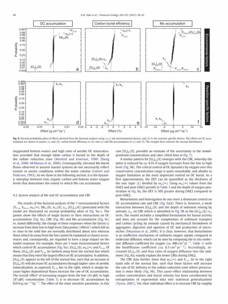
Fig. 9. Normal probability plots of effects derived from the factorial analysis using (a–c) the environmental factors, and (d–f) the reaction-specific factors. The effects on OC accu-mulation are shown in panels (a) and (d), carbon burial efficiency in (b) and (e) and Mo accumulation in (c) and (f). The straight lines indicate the normal distribution.

40 A.W. Dale et al. / Chemical Geology 324-325 (2012) 28–45

oxygenated bottom waters and high rates of aerobic OC mineraliza-tion provided that enough labile carbon is buried to the depth ofthe sulfate reduction zone (Morford and Emerson, 1999; Zhenget al., 2000; McManus et al., 2006). Consequently, elevated Mo burialfluxes observed in ancient marine systems do not necessarily reflecteuxinic or anoxic conditions within the water column (Calvert andPedersen, 1993). As we show in the following section, it is the dynam-ic interplay between iron, organic carbon and bottom water oxygenlevels that determines the extent to which Mo can accumulate.

4.3. System analysis of Mo and OC accumulation and CBE

The results of the factorial analysis of the 7 environmental factors(FC-cr, FFe-cr, ωcr(∞), Dbcr(0), αcr(0), zcr, [O2]cr(0)) generated with themodel are illustrated on normal probability plots in Fig. 9a–c. Thepanels show the effects of single factors or their interactions on OCaccumulation (Fig. 9a), CBE (Fig. 9b) and Mo accumulation (Fig. 9c)or, stated differently, the change in these responses when the factor(s)increase from their low to high level. Data points (‘effects’)which fall onor close to the solid line are normally distributed about zero whereasthosewhich lie away from the line cannot be explained as chance occur-rences and, consequently, are regarded to have a large impact on themodel response. For example, there are 3 main environmental factorswhich control OC accumulation (Fig. 9a): [O2]cr(0), ωcr(∞) and FC-cr. Ofthese, [O2]cr(0) and FC-cr lie farthest away from the normal line whichmeans that they exert the largest effect onOC accumulation. In addition,[O2]cr(0) appears to the left of the normal line, such that an increase in[O2]cr(0) will decrease OC accumulation through higher rates of aerobicmineralization, as expected. FC-cr lies to the right, which is simply be-cause higher depositional fluxes increase the rate of OC accumulation.The overall ‘effect’ of increasing oxygen from the low (61 μM) to high(87 μM) concentration (Table 3) is to decrease OC accumulation by0.014 g cm−2 ky−1. The effect of the most sensitive parameter, in this

case [O2]cr(0), provides an estimate of the uncertainty in the model-predicted concentrations and rates (thick lines in Fig. 7).

A similar pattern for [O2]cr(0) emerges with the CBE, whereby thelatter is reduced by ca. 4.5% if oxygen increases from the low to highlevel (Fig. 9b). The critical control of OC dynamics by oxygen over thisconservative concentration range is quite remarkable, and alludes tooxygen limitation as the most important control on OC burial. As afirst approximation, the OET can be quantified as the thickness ofthe oxic layer (L) divided by ωcr(∞). Using ωcr(∞) values from theOAE2 and post-OAE2 periods in Table 3 and the depth of oxygen pen-etration in Fig. 8a, the OET is 50% greater during OAE2 compared topost-OAE2.

Bioturbation and bioirrigation do not exert a dominant control onOC accumulation rate and CBE (Fig. 9a,b). There is, however, a weakinteraction between [O2]cr(0) and the depth of sediment mixing byanimals, zcr, on CBE which is identified in Fig. 9b as the [O2]cr(0)–zcrterm. The model includes a simplified formulation for faunal activityand does not account for the complexities of sediment transportand carbon cycling by animals caused by mechanical breakdown ofaggregates, digestion and egestion of OC and production of micro-niches (Meysman et al., 2006). It is clear, however, that bioturbationis an ineffective mechanism of sediment oxygen uptake compared tomolecular diffusion, which can be seen by comparing the in situ molec-ular diffusion coefficient for oxygen (ca. 400 cm2 yr−1, Table 1) withthe biodiffusion coefficient (ca. 0.5 cm2 yr−1). Accordingly, in-creased [O2]cr(0) and thus rates of oxygen diffusion into the sedi-ment (Fig. 8a) mainly explain the lower CBEs during OAE2.

The CBE data further show that ωcr(∞) and FC-cr lie to the righthand side of the normal line, such that these factors will increasethe rate of OC delivery to the sulfate reduction zone where preserva-tion is more likely (Fig. 9b). This cause–effect relationship betweencarbon concentration and burial velocity has been corroborated byextrapolation of experiential data into statistical generalizations(Tyson, 2001). Yet, their individual effect is to increase CBE by roughly

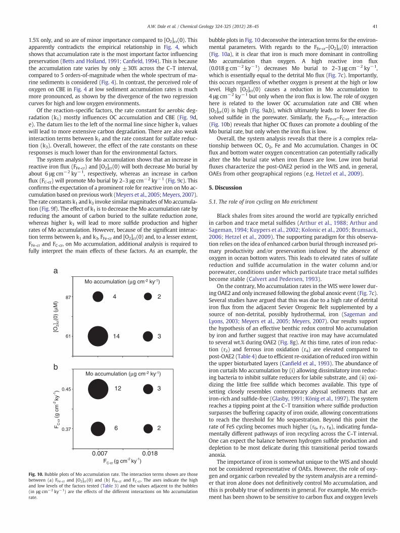
41A.W. Dale et al. / Chemical Geology 324-325 (2012) 28–45

1.5% only, and so are of minor importance compared to [O2]cr(0). Thisapparently contradicts the empirical relationship in Fig. 4, whichshows that accumulation rate is the most important factor influencingpreservation (Betts and Holland, 1991; Canfield, 1994). This is becausethe accumulation rate varies by only ±30% across the C–T interval,compared to 5 orders-of-magnitude when the whole spectrum of ma-rine sediments is considered (Fig. 4). In contrast, the perceived role ofoxygen on CBE in Fig. 4 at low sediment accumulation rates is muchmore pronounced, as shown by the divergence of the two regressioncurves for high and low oxygen environments.

Of the reaction-specific factors, the rate constant for aerobic deg-radation (k1) mostly influences OC accumulation and CBE (Fig. 9d,e). The datum lies to the left of the normal line since higher k1 valueswill lead to more extensive carbon degradation. There are also weakinteraction terms between k1 and the rate constant for sulfate reduc-tion (k3). Overall, however, the effect of the rate constants on theseresponses is much lower than for the environmental factors.

The system analysis for Mo accumulation shows that an increase inreactive iron flux (FFe-cr) and [O2]cr(0) will both decrease Mo burial byabout 6 μg cm−2 ky−1, respectively, whereas an increase in carbonflux (FC-cr) will promote Mo burial by 2–3 μg cm−2 ky−1 (Fig. 9c). Thisconfirms the expectation of a prominent role for reactive iron onMo ac-cumulation based on previouswork (Meyers et al., 2005;Meyers, 2007).The rate constants k1 and k3 invoke similarmagnitudes ofMo accumula-tion (Fig. 9f). The effect of k1 is to decrease the Mo accumulation rate byreducing the amount of carbon buried to the sulfate reduction zone,whereas higher k3 will lead to more sulfide production and higherrates of Mo accumulation. However, because of the significant interac-tion terms between k1 and k3, FFe-cr and [O2]cr(0) and, to a lesser extent,FFe-cr and FC-cr, on Mo accumulation, additional analysis is required tofully interpret the main effects of these factors. As an example, the

[O2]

cr(0

) (μ

M)

87

61

a

FC-cr (g cm-2 ky-1)

FC

-cr (g

cm

-2 ky

-1)

0.007 0.018

0.45

0.37

14 3

4 2

6 2

12 3

b

Mo accumulation (μg cm-2 ky-1)

Mo accumulation (μg cm-2 ky-1)

Fig. 10. Bubble plots of Mo accumulation rate. The interaction terms shown are thosebetween (a) FFe-cr and [O2]cr(0) and (b) FFe-cr and FC-cr. The axes indicate the highand low levels of the factors tested (Table 3) and the values adjacent to the bubbles(in μg cm−2 ky−1) are the effects of the different interactions on Mo accumulationrate.

bubble plots in Fig. 10 deconvolve the interaction terms for the environ-mental parameters. With regards to the FFe-cr–[O2]cr(0) interaction(Fig. 10a), it is clear that iron is much more dominant in controllingMo accumulation than oxygen. A high reactive iron flux(0.018 g cm−2 ky−1) decreases Mo burial to 2–3 μg cm−2 ky−1,which is essentially equal to the detrital Mo flux (Fig. 7c). Importantly,this occurs regardless of whether oxygen is present at the high or lowlevel. High [O2]cr(0) causes a reduction in Mo accumulation to4 μg cm−2 ky−1 but only when the iron flux is low. The role of oxygenhere is related to the lower OC accumulation rate and CBE when[O2]cr(0) is high (Fig. 9a,b), which ultimately leads to lower free dis-solved sulfide in the porewater. Similarly, the FFe-cr–FC-cr interaction(Fig. 10b) reveals that higher OC fluxes can promote a doubling of theMo burial rate, but only when the iron flux is low.

Overall, the system analysis reveals that there is a complex rela-tionship between OC, O2, Fe and Mo accumulation. Changes in OCflux and bottom water oxygen concentration can potentially radicallyalter the Mo burial rate when iron fluxes are low. Low iron burialfluxes characterize the post-OAE2 period in the WIS and, in general,OAEs from other geographical regions (e.g. Hetzel et al., 2009).

5. Discussion

5.1. The role of iron cycling on Mo enrichment

Black shales from sites around the world are typically enrichedin carbon and trace metal sulfides (Arthur et al., 1988; Arthur andSageman, 1994; Kuypers et al., 2002; Kolonic et al., 2005; Brumsack,2006; Hetzel et al., 2009). The supporting paradigm for this observa-tion relies on the idea of enhanced carbon burial through increased pri-mary productivity and/or preservation induced by the absence ofoxygen in ocean bottom waters. This leads to elevated rates of sulfatereduction and sulfide accumulation in the water column and/orporewater, conditions under which particulate trace metal sulfidesbecome stable (Calvert and Pedersen, 1993).

On the contrary, Mo accumulation rates in theWIS were lower dur-ing OAE2 and only increased following the global anoxic event (Fig. 7c).Several studies have argued that this was due to a high rate of detritaliron flux from the adjacent Sevier Orogenic Belt supplemented by asource of non-detrital, possibly hydrothermal, iron (Sageman andLyons, 2003; Meyers et al., 2005; Meyers, 2007). Our results supportthe hypothesis of an effective benthic redox control Mo accumulationby iron and further suggest that reactive iron may have accumulatedto several wt.% during OAE2 (Fig. 8g). At this time, rates of iron reduc-tion (r2) and ferrous iron oxidation (r4) are elevated compared topost-OAE2 (Table 4) due to efficient re-oxidation of reduced ironwithinthe upper bioturbated layers (Canfield et al., 1993). The abundance ofiron curtails Mo accumulation by (i) allowing dissimilatory iron reduc-ing bacteria to inhibit sulfate reducers for labile substrate, and (ii) oxi-dizing the little free sulfide which becomes available. This type ofsetting closely resembles contemporary abyssal sediments that areiron-rich and sulfide-free (Glasby, 1991; König et al., 1997). The systemreaches a tipping point at the C–T transition where sulfide productionsurpasses the buffering capacity of iron oxide, allowing concentrationsto reach the threshold for Mo sequestration. Beyond this point therate of FeS cycling becomes much higher (r6, r7, r8), indicating funda-mentally different pathways of iron recycling across the C–T interval.One can expect the balance between hydrogen sulfide production anddepletion to be most delicate during this transitional period towardsanoxia.

The importance of iron is somewhat unique to theWIS and shouldnot be considered representative of OAEs. However, the role of oxy-gen and organic carbon revealed by the system analysis are a remind-er that iron alone does not definitively control Mo accumulation, andthis is probably true of sediments in general. For example, Mo enrich-ment has been shown to be sensitive to carbon flux and oxygen levels

0.2 0.3 0.4 0.5 0.6

OC flux (g C cm-2kyr-1)

40

60

80

100

120

Bot

tom

wat

er o

xyge

n co

ncen

trat

ion

(μM

)

Fig. 11. Reconstructed bottom water oxygen concentrations versus reconstructedorganic carbon fluxes across the C–T interval.

42 A.W. Dale et al. / Chemical Geology 324-325 (2012) 28–45

in modern surface sediments along the oxygenminimum zones of theAmericas (McManus et al., 2006; Scholz et al., 2011). Due consider-ation of coupled iron, carbon and oxygen cycling is critical to inter-preting paleoredox indicators such as Mo.

Adsorption of MoO42− onto iron (andmanganese) oxyhydroxides in

oxic waters (Helz et al., 1996) and deposition on the seafloor providesan additional mechanism for Mo transfer to the sediment in additionto diffusion from sea water (Crusius et al., 1996). Subsequent reductivedissolution of the iron oxides releases Mo to anoxic sediment pore-waters, which can then be sequestered and precipitated as thiomolyb-date or diffuse back to the water column. In general, this transferpathway is small compared to the diffusiveMo flux across the sedimentwater interface (Crusius et al., 1996; Erickson and Helz, 2000; Zhenget al., 2000). However, iron-associated Mo may lead to strong benthicenrichment of authigenic Mo in silled basins with weakly or seasonallyanoxic bottom waters where the chemocline migrates through thesediment–water interface (Algeo and Lyons, 2006). These settings areparticularly susceptible to Mo trapping because repeated ventilationof the deep water catalyzes the re-oxidation of dissolved iron andman-ganese to particulate oxyhydroxides, thus recreating the necessary con-ditions for a new flux of adsorbedMo. This hypothetical ‘Mo pump’wasconceived to explain sedimentary Mo concentrations in excess of100 ppm in modern basins such as Saanich Inlet and Cariaco Basin(Algeo and Lyons, 2006). Given the abundance of iron in the WIS, onewould expect to see the Bridge Creek data punctuated with extremeMo enrichments if the Mo pump was periodically active. However,such enrichments are absent from both the 2 meter smoothed Mo con-centrations (b10 ppm, Fig. 7f) and the raw data (max. 20 ppm, data notshown). For this reason, we exclude this mechanism as a vector for Moenrichment in the WIS.

5.2. Production versus preservation of OC across the C–T interval

Increased global burial of OC during OAE2 is usually inferred from themarked positive excursion in δ13COC and δ13CCaCO3 followed by a returnto more negative values in the post-OAE2 period as paleoproductionand OC burial decreased (Arthur et al., 1988). The Bridge Creek δ13COCdata essentially track the trend of the global ocean (Sageman et al.,2006). Yet, the striking increase in OC concentration and accumulationrates occurring after OAE2 (Fig. 7) suggests that the extent and timingof ‘OAE2-like’ conditions in the shallow epicontinental WIS were offsetfrom the rest of the ocean (Meyers et al., 2001; Sageman and Lyons,2003). To help identify the contribution of productivity and preserva-tion on OC accumulation in the WIS, Meyers et al. (2001; 2005)employed carbonate accumulation as a qualitative proxy for paleopro-duction (Fig. 1d). The lower carbonate accumulation rates post-OAE2were inferred to represent lower paleoproductivity, and the OC enrich-ment relative to OAE2was thus explained as carbon preservation. In ac-cordance with this idea, they adopted a simple preservation scalingapproach, that is, dividing the carbon accumulation rate by the FOL,which predicted lower rates of paleoproduction post-OAE2 comparedto OAE2. These researchers went on to argue that OC preservationwas driven by (i) a decline in reactive iron flux which led to increaseddissolved sulfide concentrations in the porewater, reduced bioturbationdue to faunal toxicity to sulfide and a shallower sulfate reduction zone(thinner oxic layer), and (ii) a reduction in bulk sediment dilution.Equally, less OC preservation occurred during OAE2 because the de-crease in sulfide levels by iron buffering led tomore efficient ventilationof the sediments by burrowing animals; a hypothesis later termed the‘sulfide buffer/phosphorus trap’ (Meyers, 2007). However, despite theobvious role of iron on Mo accumulation (see above), our analysisdoes not indicate any substantial role for iron on OC accumulation(Fig. 9a). Instead, our results which are based on a more rigorous esti-mate of reconstructed carbon flux allude to the combined effects ofpaleoproduction and preservation,whereby amodest increase in paleo-production (i.e. higher FC-Cr) in conjunction with preservation (i.e.

lower [O2]cr(0)), conspired to allow OC (and Mo) to accumulate athigher rates post-OAE2 andwith a higher CBE. A plot of [O2]cr(0) versusFC-Cr (Fig. 11) shows the inverse relationship between the two factorsacross the C–T interval. We reiterate that this result is by no means certaindue to the inherent uncertainties in reconstructing the boundary conditionsof theWIS sediments. It does, however, illustrate howsimultaneous produc-tion andpreservation can give rise to geochemical trends that are character-istic of OAE-like conditions.

The use of carbonate as a paleoproductivity proxy assumes thatthe phytoplankton composition remained relatively uniform in thecentral WIS over the C–T interval and that carbonate dissolutionand precipitation were constant over time (Meyers et al., 2005). Themodel results presented here provide circumstantial evidence thatthe latter condition may not have been fulfilled. To explain, the diage-netic regimes between OAE2 and post-OAE2 are radically different(Fig. 8), being highly ferruginous during OAE2 and sulfidic thereafter.There is a transition from dissimilatory iron reduction and net sulfidebuffering toward sulfate reduction and sulfide accumulation betweenthe two periods. Critically, the number of protons, or alkalinity equiv-alents, produced and consumed by these reactions is different (ΔTA,Table 4). Stoichiometrically, much more alkalinity is produced by dis-similatory iron reduction (+8 equivalents per mole of carbon oxi-dized) compared to sulfate reduction (+1). Despite the small netproduction of alkalinity during OAE2 (+0.14 eq m−2 yr−1), it is verylikely that carbonate minerals were in a state of disequilibrium in thesurface sediments. For instance, dissimilatory iron reduction (r3) pro-duces +23.1 eq m−2 yr−1 of alkalinity, which will favor carbonatepreservation and possibly authigenic carbonate precipitation in theselayers. However, ferrous iron oxidation consumes 23 eq m−2 ky−1 ofalkalinity, which will lead to highly undersaturated pore waters withinthe thin upper oxic layer (Jourabchi et al., 2005). Since the rate of car-bonate dissolution depends on the mineral saturation state (e.g. Keir,1980), which in turn depends on the porewater alkalinity and pH, thisreaction creates a strong thermodynamic drive for carbonate dissolu-tion in the surface layers.

The post-OAE2 sediments are associated with a larger net alkalin-ity production (2.8 eq m−2 yr−1 of alkalinity), which is due to burialof FeS. Again, one may expect sulfide oxidation reactions in thesurface layers to cause an undersaturation with respect to car-bonate minerals. Furthermore, the depth-integrated rate of aero-bic OC mineralization post-OAE2 and, therefore, CO2 production is

43A.W. Dale et al. / Chemical Geology 324-325 (2012) 28–45

46 mol m−2 yr−1 higher than during OAE2. Although this reactiondoes not affect total alkalinity directly, CO2 will rapidly neutralize car-bonate ion alkalinity (CO2+CO3

2−+H2O→2HCO32−) and lower the

carbonate saturation state. This ‘metabolic dissolution’, to distinguishfrom thermodynamically-driven dissolution, is a common character-istic of surface marine sediments (Emerson and Bender, 1981; Archeret al., 1989) and could conceivably account for the lower rates ofcalcite accumulation post-OAE2. This cautions against the use ofcarbonate content as a proxy for primary production. A more sophis-ticated model than the one presented here would be required to testthis idea more rigorously (Jourabchi et al., 2008).

In summary, the above calculations highlight the difficulties in dis-entangling the role of production and preservation through a qualita-tive interpretation of carbonate accumulation rates where there arelarge shifts in benthic redox potential. Erba (2004) raised similar con-cerns for the interpretation of calcareous nannofossils in black shales.The interpretation of proxies through the application of models usinghighly resolved data from OAE2 sequences elsewhere (e.g. Kolonicet al., 2005; Hetzel et al., 2009) shows great promise in delivering amore global picture of the significance of benthic processes duringthe onset of ocean anoxia.

6. Conclusions

Proxy signals recorded in marine sediments can be amplified or di-minished by changes in the intensity of physical processes (e.g. burialrates, bioturbation) as well as biogeochemical reactions. Benthic cyclesare highly coupled through the chemical species and can interact syner-gistically or antagonistically on the accumulation of key geochemical in-dicators. It thus becomes challenging, if not impossible, to adduce themajor forcings by a qualitative analysis of the data. Reaction-transportmodels integrate transport processes and biogeochemistry into a quan-titative framework and can be used to extricate the overarching con-trols on single- or multi-proxy inventories.

We applied a model to reconstruct the geochemical paleorecordpreserved in strata of the Bridge Creek Limestone Member of theWestern Interior Seaway and evaluate the controls on organic carbon(OC) andmolybdenum (Mo) accumulation rate. Our attention focused onthe Cenomanian–Turonian (C–T) boundary interval (94.34–93.04 Ma)which includesOAE2. To our knowledge, this is thefirstmodel applicationto reconstructmulti-proxy data recorded in fully consolidated sedimen-tary rock. This approach thus represents a new dimension for studyingdeep-time biogeochemical processes in a dynamic manner.

Important implications follow from thiswork. Our results clearly cor-roborate Meyers' (2007) argument that the accumulation rate of partic-ulate Mo in black shales is a poor proxy for ocean euxinia or even anoxiain ancient marine systems.We show that high rates of Mo accumulationcan occur with high rates of aerobic OC degradation in the surface sedi-ments. Furthermore, Mo sequestration can be severely restricted by theavailability of reactive iron oxides which buffer porewater sulfide tolevels below those required for Mo sequestration. Evidence suggeststhat the bottomwaters became progressively more hypoxic, but not an-oxic, over the C–T interval in the WIS in parallel with increasing OC fluxto the seafloor. This alludes to a positive feedback between the sea floorand the photic zone, probably via phosphate, on the advance of anoxia.Future modeling work will address this hypothesis by incorporatingphosphorous data into the model. The results presented simultaneouslysupport both long-standing notions that OC enrichment in ancient sedi-ments is driven by increased preservation and increased export produc-tion. There is no reason why these should be regarded as uncoupled,independent processes.

Acknowledgments

We are grateful for the useful comments of two reviewers andthe guest Editor Jennifer Morford which improved the paper. The

Deutsche Forschungsgemeinschaft provided support as part of theSonderforschungsbereich 754 (http://www.sfb754.de). S.A. acknowl-edges financial support from NERC (Grant No. NE/I021322/1).

References

Adams, D.D., Hurtgen, M.T., Sageman, B.B., 2010. Volcanic triggering of a biogeochem-ical cascade during Oceanic Anoxic Event 2. Nature Geoscience 3, 201–204.

Algeo, T.J., Lyons, T.W., 2006. Mo-total organic carbon covariation in modern anoxicmarine environments: implications for analysis of paleoredox and paleohydro-graphic conditions. Paleoceanography 21, PA1016. doi:10.1029/2004PA001112.

Archer, S., Emerson, S., Reimers, C., 1989. Dissolution of calcite in deep-sea sedi-ments: pH and O2 microelectrode results. Geochimica et Cosmochimica Acta53, 2831–2845.

Arndt, S., Hetzel, A., Brumsack, H.J., 2009. Evolution of organic matter degradation inCretaceous black shales inferred from authigenic barite: a reaction-transportmodel. Geochimica et Cosmochimica Acta 73, 2000–2022.

Arthur, M.A., Schlanger, S.O., Jenkyns, H.C., 1987. The Cenomanian–Turonian OceanicAnoxic Event, II. Palaeoceanographic controls on organic-matter production andpreservation. In: Brooks, J., Fleet, A.J. (Eds.), Marine Petroleum Source Rocks. : Geo-logical Society Special Publication, 26. Blackwell, Oxford, pp. 401–420.

Arthur, M.A., Dean, W.E., Pratt, L.M., 1988. Geochemical and climatic effects of in-creased marine organic carbon burial at the Cenomanian/Turonian boundary. Na-ture 335, 714–717.

Arthur, M.A., Sageman, B.B., 1994. Marine black shales: depositional mechanisms andenvironments of ancient deposits. Annual Review of Earth and Planetary Sciences22, 499–551.

Barron, E.J., 1983. A warm, equable Cretaceous: the nature of the problem. Earth-ScienceReviews 19, 305–338.

Berelson, W.M., Hammond, D.E., Johnson, K.S., 1987. Benthic fluxes and the cycling ofbiogenic silica and carbon in two southern California borderland basins. Geochi-mica et Cosmochimica Acta 51, 1345–1363.

Berg, P., Rysgaard, S., Thamdrup, B., 2003. Dynamic modeling of early diagenesis andnutrient cycling. A case study in an Arctic marine sediment. American Journal ofScience 303, 905–955.

Berner, R.A., 1980. Early Diagenesis: A Theoretical Approach. Princeton UniversityPress, Princeton. 241 pp.

Berner, R.A., 1982. Burial of organic carbon and pyrite sulfur in the modern ocean; itsgeochemical and environmental significance. American Journal of Science 282,451–473.

Betts, J.N., Holland, H.D., 1991. The oxygen content of ocean bottom waters, the burialefficiency of organic carbon, and the regulation of atmospheric oxygen. Palaeogeo-graphy, Palaeoclimatology, Palaeoecology 97, 5–18.

Bohlen, L., Dale, A.W., Sommer, S.,Mosch, T., Hensen, C., Noffke, A., Scholz, F.,Wallmann, K.2011. Benthic nitrogen cycling traversing the Peruvian oxygen minimum zone. Geo-chimica et Cosmochimica Acta, 75, 6094–6111.

Böning, P., Brumsack, H.J., Böttcher, M.E., Schnetger, B., Kriete, C., Kallmeyer, J., Borch-ers, S.L., 2004. Geochemistry of Peruvian near-surface sediments. Geochimica etCosmochimica Acta 68, 4429–4451.

Boudreau, B.P., 1991. Modelling the sulfide–oxygen reaction and associated pH gradientsin porewaters. Geochimica et Cosmochimica Acta 55, 145–159.

Boudreau, B.P., 1996. A method-of-lines code for carbon and nutrient diagenesis inaquatic sediments. Computers and Geosciences 22, 479–496.

Boudreau, B.P., 1997. Diagenetic Models and Their Implementation: Modelling Trans-port and Reactions in Aquatic Sediments. Springer-Verlag, Berlin. 414 pp.

Box, G.E.P., Hunter, W.G., Hunter, J.S., 1978. Statistics for Experimenters. An Introduc-tion to Design, Data Analysis and Model Building. Wiley, New York. 653 pp.

Bralower, T.J., Thierstein, H.R., 1984. Low productivity and slow deep-water circulationin mid-Cretaceous oceans. Geology 12, 614–618.

Brigolin, D., Pastres, R., Nickell, T.D., Cromey, C.J., Aguilera, D.R., Regnier, P., 2009. Model-ling the impact of aquaculture on early diagenetic processes in sea loch sediments.Marine Ecology Progress Series 388, 63–80.

Brumsack, H.J., 2006. The trace metal content of recent organic carbon-rich sediments:implications for Cretaceous black shale formation. Palaeogeography, Palaeoclima-tology, Palaeoecology 232, 344–361.

Burdige, D.J., 2006. Geochemistry of Marine Sediments. Princeton Univ Press,Princeton, N. J.

Burdige, D.J., 2007. Preservation of organic matter in marine sediments: controls, mecha-nisms, and an imbalance in sediment organic carbon budgets? Chemical Reviews 107,467–485.

Calvert, S.E., Pedersen, T.F., 1993. Geochemistry of recent oxic and anoxic marine sed-iments: implications for the geological record. Marine Geology 113, 67–88.

Canavan, R.W., Slomp, C.P., Jourabchi, P., Van Cappellen, P., Laverman, A.M., van denBerg, G.A., 2006. Organic matter mineralization in sediment of a coastal fresh-water lake and response to salinization. Geochimica et Cosmochimica Acta 70,2836–2855.

Canfield, D.E., 1993. Organic matter oxidation in marine sediments. In: Wollast, R.,Mackenzie, F.T., Chou, L. (Eds.), Interactions of C, N, P and S Biogeochemical Cyclesand Global Change. : NATO ASI Ser., Ser. I, vol. 4. Springer, Berlin, pp. 333–364.

Canfield, D.E., 1994. Factors influencing organic carbon preservation in marine sediments.Chemical Geology 114, 315–329.

Canfield, D.E., Thamdrup, B., Hansen, J.W., 1993. The anaerobic degradation of organicmatter in Danish coastal sediments: iron reduction,manganese reduction, and sulfatereduction. Geochimica et Cosmochimica Acta 57, 3867–3883.

44 A.W. Dale et al. / Chemical Geology 324-325 (2012) 28–45

Crusius, J., Calvert, S., Pedersen, T., Sage, D., 1996. Rhenium and molybdenum enrich-ments in sediments as indicators of oxic, suboxic and sulfidic conditions of deposi-tion. Earth and Planetary Science Letters 145, 65–78.

Dale, A.W., Regnier, P., Van Cappellen, P., 2006. Bioenergetic controls on anaerobic ox-idation of methane (AOM) in coastal marine sediments: a theoretical analysis.American Journal of Science 306, 246–294.

Dale, A.W., Brüchert, V., Alperin, M., Regnier, P., 2009. An integrated sulfur isotopemodel for Namibian shelf sediments. Geochimica et Cosmochimica Acta 73,1924–1944.

Dale, A.W., Sommer, S., Bohlen, L., Treude, T., Bertics, V.J., Bange, H.W., Pfannkuche, O.,Schorp, T., Mattsdotter, M., Wallmann, K., 2011. Rates and regulation of nitrogencycling in seasonally hypoxic sediments during winter (Boknis Eck, SW BalticSea): sensitivity to environmental variables. Estuarine, Coastal and Shelf Science95, 14–28.

Dean, W.E., Arthur, M.A., 1989. Iron–sulfur–carbon relationships in organic-carbon-richsequences I: CretaceousWestern Interior Seaway. American Journal of Science 289,708–743.

Demaison, G.J., Moore, G.T., 1980. Anoxic environments and oil source bed genesis.American Association of Petroleum Geologists Bulletin 64, 1179–1209.

Dhakar, S.P., Burdige, D.J., 1996. A coupled, non-linear, steady-state model for early dia-genetic processes in pelagic sediments. American Journal of Science 296, 296–330.

Diaz, R.J., Rosenberg, R., 1995. Marine benthic hypoxia — review of ecological effectsand behavioral responses on macrofauna. Oceanography and Marine Biology: AnAnnual Review 33, 245–303.

Elder, W.P., Gustason, E.R., Sageman, B., 1994. Basinwide correlation of parasequencesin the Greenhorn Cyclothem, Western Interior, U.S. Geological Society of AmericaBulletin 106, 892–902.

Eldridge, P.M., Morse, J.W., 2000. A diagenetic model for sediment–seagrass interac-tions. Marine Chemistry 70, 89–103.

Emerson, S., Jahnke, R., Bender, M., Froelich, P., Klinkhammer, G., Bowser, C., Setlock, G.,1980. Early diagenesis in sediments from the eastern equatorial Pacific. I. Porewater nutrient and carbonate results. Earth and Planetary Science Letters 49, 57–80.

Emerson, S., Bender, M., 1981. Carbon fluxes at the sediment–water interface of the deepsea — calcium carbonate preservation. Journal of Marine Research 39, 139–162.

Erba, E., 2004. Calcareous nannofossils and Mesozoic oceanic anoxic events. MarineMicropaleontology 52, 85–106.

Erickson, B.E., Helz, G.R., 2000. Molybdenum(VI) speciation in sulfidic waters: stabilityand lability of thiomolybdates. Geochimica et Cosmochimica Acta 64, 1149–1158.

Fisher, C.G., Arthur, M.A., 2002. Water mass characteristics in the Cenomanian USWestern Interior seaway as indicated by stable isotopes of calcareous organisms.Palaeogeography, Palaeoclimatology, Palaeoecology 188, 189–213.

Fossing, H., Berg, P., Thamdrup, B., Rysgaard, S., Sřrensen, H.M., Nielsen, K., 2004. A modelset-up for an oxygen and nutrient fluxmodel for Aarhus Bay (Denmark). National En-vironmental Research Institute (NERI), Technical Report, No. 483. . 68 pp.

Froelich, P.N., Klinkhammer, G.P., Bender, M.L., Luedtke, N.A., Heath, G.R., Cullen, D.,Dauphin, P., 1979. Early oxidation of organic matter in pelagic sediments of theeastern equatorial Atlantic: suboxic diagenesis. Geochimica et CosmochimicaActa 43, 1075–1090.

Furukawa, Y., Smith, A.C., Kostka, J.E., Watkins, J., Alexander, C.R., 2004. Quantificationof macrobenthic effects on diagenesis using a multicomponent inverse model insalt marsh sediments. Limnology and Oceanography 49, 2058–2072.

Glasby, G.P., 1991. Mineralogy and geochemistry of Pacific red clays. New Zealand Journalof Geology and Geophysics 34, 167–176.

Glud, R.N., Gundersen, J.K., Jørgensen, B.B., Revsbech, N.P., Schulz, H.D., 1994. Diffusiveand total oxygen uptake of deep-sea sediments in the eastern South AtlanticOcean: in situ and laboratory measurements. Deep-Sea Research II 41, 1767–1788.

Goldberg, T., Archer, C., Vance, D., Poulton, S.W., 2009.Mo isotope fractionation during ad-sorption to Fe (oxyhydr)oxides. Geochimica et Cosmochimica Acta 73, 6502–6516.

Haeckel, M., König, I., Riech, v., Weber, M.E., Suess, E., 2001. Pore water profiles and nu-merical modelling of biogeochemical processes in Peru Basin deep-sea sediments.Deep-Sea Research II 48, 3713–3736.

Hartnett, H.E., Devol, A.H., 2003. Role of a strong oxygen-deficient zone in the preservationand degradation of organic matter: a carbon budget for the continental margins ofnorthwest Mexico and Washington State. Geochimica et Cosmochimica Acta 67,247–264.

Hebting, Y., Schaeffer, P., Behrens, A., Adam, P., Schmitt, G., Schneckenburger, P., Bernasconi,S.M., Albrecht, P., 2006. Biomarker evidence for a major preservation pathway of sedi-mentary organic carbon. Nature 312, 1627–1631.

Hedges, J.I., Keil, R.G., 1995. Sedimentary organic matter preservation: an assessmentand speculative synthesis. Marine Chemistry 49, 81–115.

Helz, G.R., Miller, C.V., Charnock, J.M., Mosselmans, J.F.W., Pattrick, R.A.D., Garner, C.D.,Vaughan, D.J., 1996. Mechanism of molybdenum removal from the sea and its con-centration in black shales: EXAFS evidence. Geochimica et Cosmochimica Acta 60,3631–3642.

Hetzel, A., Böttcher, M.E., Wortmann, U.G., Brumsack, H.J., 2009. Paleo-redox conditionsduring OAE 2 reflected in Demerara Rise sediment geochemistry (ODP Leg 207).Palaeogeography, Palaeoclimatology, Palaeoecology 273, 302–328.

Horita, J., Zimmermann, H., Holland, H.D., 2002. Chemical evolution of seawater duringthe Phanerozoic: implications from the record of marine evaporites. Geochimica etCosmochimica Acta 66, 3733–3756.

Ingall, E., Jahnke, R., 1997. Influence ofwater-columnanoxia on the elemental fractionationof carbon and phosphorus during sediment diagenesis. Marine Geology 139, 219–229.

Jahnke, J., Heggie, D., Emerson, S., Grundmanis, V., 1982. Pore waters of the central PacificOcean: nutrient results. Earth and Planetary Science Letters 61, 233–256.

Jenkyns, H.C., 2010. Geochemistry of oceanic anoxic events. Geochemistry, Geophysics,Geosystems 11, Q03004. doi:10.1029/2009GC002788.

Jørgensen, B.B., 1977. The sulfur cycle of a coastalmarine sediment (Limfjorden, Denmark).Limnology and Oceanography 22, 814–832.

Jørgensen, B.B., Kasten, S., 2006. Sulfur cycling and methane oxidation, In: Schulz, H.D.,Zabel, M. (Eds.), Marine Geochemistry, 2nd ed. Springer–Verlag, Berlin, pp. 271–309.

Jourabchi, P., Van Cappellen, P., Regnier, P., 2005. Quantitative interpretation of pH distri-butions in aquatic sediments: a reaction-transport modeling approach. AmericanJournal of Science 305, 919–956.

Jourabchi, P., Meile, C., Pasion, L.R., Van Cappellen, P., 2008. Quantitative interpretation ofporewaterO2 andpHdistributions in deep-sea sediments. Geochimica et CosmochimicaActa 72, 1350–1364.

Katsev, S., Sundby, B., Mucci, A., 2006. Modeling vertical excursions of the redoxboundary in sediments: application to deep basins of the Arctic Ocean. Limnologyand Oceanography 51, 1581–1593.

Katsev, S., Chaillou, G., Sundby, B., Mucci, A., 2007. Effects of progressive oxygen depletionon sediment diagenesis and fluxes: a model for the lower St Lawrence River Estuary.Limnology and Oceanography 52, 2555–2568.

Kauffman, E.G., 1977. Geological and biological overview: Western Interior CretaceousBasin. Mountain Geologist 13, 75–99.

Keeling, R.F., Körtzinger, A., Gruber, N., 2010. Ocean deoxygenation in a warmingworld. Annual Review of Marine Science 2, 199–229.

Keir, R.A., 1980. The dissolution kinetics of biogenic calcium carbonates in seawater.Geochimica et Cosmochimica Acta 44, 241–252.

Kolonic, S., Wagner, T., Forster, A., Sinninghe Damsté, J.S., Walsworth-Bell, B., Erba, E.,Turgeon, S., Brumsack, H.J., Chellai, E.H., Tsikos, H., Kuhnt, W., Kuypers, M.M.M.,2005. Black shale deposition on the northwest African Shelf during the Cenomanian/Turonian Oceanic Anoxic Event: climate coupling and global organic carbon burial.Paleoceanography 20, PA1006. doi:10.1029/2003PA000950.

König, I., Drodt, M., Suess, E., Trautwein, A.X., 1997. Iron reduction through the tan–greencolor transition in deep-sea sediments. Geochimica et Cosmochimica Acta 61,1679–1683.

König, I., Haeckel, M., Drodt, M., Suess, E., Trautwein, A.X., 1999. Reactive Fe(II) layers indeep-sea sediments. Geochimica et Cosmochimica Acta 63, 1517–1526.

Kraal, P., Slomp, C.P., Forster, A., Kuypers, M.M.M., 2010. Phosphorus cycling from themargin to abyssal depths in the proto-Atlantic during Oceanic Anoxic Event 2.Palaeogeography, Palaeoclimatology, Palaeoecology 295, 42–54.

Kump, L.R., Slingerland, R.L., 1999. Circulation and stratification of the early TuronianWestern Interior Seaway: sensitivity to a variety of forcings. In: Barrera, E., John-son, C.C. (Eds.), The Evolution of the Cretaceous Ocean–Climatic System. Geol.Soc. Am, Boulder, Colorado, pp. 181–190.

Kuypers, M.M.M., Pancost, R.D., Nijenhuis, I.A., Sinninghe Damsté, J.S., 2002. Enhancedproductivity led to increased organic carbon burial in the euxinic North Atlanticbasin during the late Cenomanian Oceanic Anoxic Event. Paleoceanography 17,1051. doi:10.1029/2000PA000569.

Levin, L.A., 2003. Oxygenminimumzone benthos: adaptation and community response tohypoxia. Oceanography and Marine Biology: An Annual Review 41, 1–45.

Linke, P., Wallmann, K., Suess, E., Hensen, C., Rehder, G., 2005. In situ benthic fluxesfrom an intermittently active mud volcano at the Costa Rica convergent margin.Earth and Planetary Science Letters 235, 79–95.

Martin, W.R., Sayles, F.L., 2006. Organic matter oxidation in deep-sea sediments: distri-bution in the sediment column and implications for calcite dissolution. Deep-SeaResearch II 53, 771–792.

McManus, J., Berelson, W.M., Severmann, S., Poulson, R.L., Hammond, D.E., Klinkhammer,G.P., Holm, C., 2006. Molybdenum and uranium geochemistry in continental marginsediments: paleoproxy potential. Geochimica et Cosmochimica Acta 70, 4643–4662.

Meile, C., Van Cappellen, P., 2005. Particle age distributions and O2 exposure times:timescales in bioturbated sediments. Global Biogeochemical Cycles 19, GB3013.doi:10.1029/2004GB002371.

Meyers, S.R., 2007. Production and preservation of organic matter: the significance ofiron. Paleoceanography 22, PA4211. doi:10.1029/2006PA001332.

Meyers, S.R., Sageman, B.B., 2007. Quantification of deep-time orbital forcing by averagespectral misfit. American Journal of Science 307, 773–792.

Meyers, S.M., Sageman, B.B., Hinnov, L.A., 2001. Integrated quantitative stratigraphy ofthe Cenomanian–Turonian Bridge Creek LimestoneMember using evolutive harmonicanalysis and stratigraphic modeling. Journal of Sedimentary Research 71, 628–644.doi:10.1306/012401710628.

Meyers, S.R., Sageman, B.B., Lyons, T.W., 2005. Organic carbon burial rate and themolybdenum proxy: theoretical framework and application to Cenomanian–Turonian oceanic anoxic event 2. Paleoceanography 20, PA2002. doi:10.1029/2004PA001068.

Meyers, S.R., Siewert, S.E., Singer, B.S., Sageman, B.B., Condon, D.J., Obradovich, J.D.,Jicha, B.R., Sawer, D.A., in press. Intercalibration of radioisotopic and astrochrono-logic time scales for the Cenomanian-Turonian boundary interval, Western InteriorBasin, USA. Geology. doi:10.1130/G32261.1.

Meysman, F.J.R., Middelburg, J.J., Herman, P.M.J., Heip, C.H.R., 2003. Reactive transportin surface sediments. II. Media: an object-oriented problem-solving environmentfor early diagenesis. Computers and Geosciences 29, 301–318.

Meysman, F.J.R., Middelburg, J.J., Heip, C.H.R., 2006. Bioturbation: a fresh look at Darwin'slast idea. Trends in Ecology & Evolution 21, 688–695.

Middelburg, J.J., 1989. A simple rate model for organic matter decomposition in marinesediments. Geochimica et Cosmochimica Acta 53, 1577–1581.

Middelburg, J.J., Levin, L.A., 2009. Coastal hypoxia and sediment biogeochemistry.Biogeosciences 6, 1273–1293.

Middelburg, J.J., Soetaert, K., Herman, P.M.J., 1997. Empirical relationships for use inglobal diagenetic models. Deep-Sea Research I 44, 327–344.

Middelburg, J.J., Vlug, T., Jaco, F., van der Nat, W.A., 1993. Organic matter mineralizationin marine systems. Global and Planetary Change 8, 47–58.

45A.W. Dale et al. / Chemical Geology 324-325 (2012) 28–45

Millero, F.J., Hubinger, S., Fernandez,M., Garnett, S., 1987a. Oxidation of H2S in seawater asa function of temperature, pH, and ionic strength. Environmental Science and Tech-nology 21, 439–443.

Millero, F.J., Sotolongo, S., Izaguirre,M., 1987b. The oxidation kinetics of Fe(II) in seawater.Geochimica et Cosmochimica Acta 51, 793–801.

Moodley, L., Middelburg, J.J., Herman, P.M.J., Soetaert, K., de Lange, G.J., 2005. Oxygenationand organic-matter preservation in marine sediments: direct experimental evidencefrom ancient organic carbon-rich deposits. Geology 33, 889–892.

Morford, J.L., Emerson, S. The, 1999. geochemistry of redox sensitive trace metals insediments. Geochimica et Cosmochimica Acta 63, 1735–1750.

Morford, J.L., Martin, W.R., Francois, R., Carney, C.M., 2009. A model for uranium, rheni-um, and molybdenum diagenesis in marine sediments based on results from coast-al locations. Geochimica et Cosmochimica Acta 73, 2938–2960.

Niggemann, J., Ferdelman, T.G., Lomstein, B.A., Kallmeyer, J., Schubert, C.J., 2007. How de-positional conditions control input, composition, and degradation of organicmatter insediments from the Chilean coastal upwelling region. Geochimica et CosmochimicaActa 71, 1513–1527.

Pedersen, T.F., Calvert, S.E., 1990. Anoxia vs productivity—what controls the formationof organic carbon-rich sediments and sedimentary rocks. American Association ofPetroleum Geologists Bulletin 74, 454–466.

Poulton, S.W., Raiswell, R., 2002. The low-temperature geochemical cycle of iron: fromcontinental fluxes to marine sediment deposition. American Journal of Science 302,774–805.

Pratt, L.M., 1985. Isotopic studies of organic matter and carbonate in rocks of theGreenhorn marine cycle. In: Pratt, L.M., Kauffman, E.G., Zelt, F.B. (Eds.), Fine-grained Deposits and Biofacies of the Cretaceous Western Interior Seaway: Evi-dence of Cyclic Sedimentary Processes: SEPM Field Trip Guidebook, 4, pp. 38–48.

Pyzik, A.J., Sommer, S.E., 1981. Sedimentary iron monosulfides: kinetics and mecha-nism of formation. Geochimica et Cosmochimica Acta 45, 687–698.

Raiswell, R., Canfield, D.E., 1996. Rates of reaction between silicate iron and dissolved sul-fide in Peru Margin sediments. Geochimica et Cosmochimica Acta 60, 2777–2787.

Reimers, C.E., Fischer, K.M., Merewether, R., Smith, K.L., Jahnke, R.A., 1986. Oxygenmicroprofiles measured in situ in deep ocean sediments. Nature 320, 741–744.

Sageman, B.B., Arthur, M.A., 1994. Early Turonian paleogeographic/paleobathymetricmap, Western Interior, U.S. In: Caputo, M., Peterson, J., Franczyk, K. (Eds.), MesozoicSystems of the Rocky Mountain Region: SEPM, Special Publication, pp. 457–470.

Sageman, B.B., Lyons, T.W., 2003. Geochemistry offine-grained sediments and sedimentaryrocks. In: Holland, H.D., Turekian, K.K. (Eds.), Treatise on Geochemistry, Volume 7.Elsevier, pp. 115–158.

Sageman, B.B., Meyers, S.R., Arthur, M.A., 2006. Orbital time scale and new C-isotoperecord for Cenomanian–Turonian boundary stratotype. Geology 34, 125–128.

Sageman, B.B., Rich, J., Arthur, M.A., Birchfield, G.E., Dean, W.E., 1997. Evidence forMilankovitch periodicities in Cenomanian–Turonian lithologic and geochemicalcycles, Western Interior U.S. Journal of Sedimentary Research 67, 286–301.

Schlanger, S.O., Jenkyns, H.C., 1976. Cretaceous oceanic anoxic events: causes andconsequences. Geologie en Mijnbouw 55, 179–184.

Schlanger,M.A., Arthur,M.A., Jenkyns, H.C., Scholle, P.A., 1987. The Cenomanian–TuronianOceanic Anoxic Event, I. Stratigraphy and distribution of organic carbon-rich beds andthe marine δ13C excursion. In: Brooks, J., Fleet, A.J. (Eds.), Marine Petroleum SourceRocks. : Geological Society Special Publication, 26. Blackwell, Oxford, pp. 371–399.

Scholz, F., Hensen, C., Noffke, A., Rohde, A., Liebetrau, V.,Wallmann, K., 2011. Early diagenesisof redox-sensitive trace metals in the Peru upwelling area — response to ENSO-relatedoxygen fluctuations in thewater column. Geochimica et Q8 Cosmochimica Acta 75,7257–7276.

Schulz, H.D., 2000. Quantification of early diagenesis: dissolved constituents in marinepore water. In: Schulz, H.D., Zabel, M. (Eds.), Marine Geochemistry. Springer-Verlag,Berlin, pp. 85–128.

Seiter, K., Hensen, C., Zabel, M., 2005. Benthic carbon mineralization on a global scale.Global Biogeochemical Cycles 19, GB1010. doi:10.1029/2004GB002225.

Slingerland, R., Kump, L.R., Arthur, M.A., Fawcett, P.J., Sageman, B.B., Barron, E.J., 1996.Estuarine circulation in the Turonian Western Interior seaway of North America.Geological Society of America Bulletin 108, 941–952.

Snow, L.J., Duncan, R.A., Bralower, T.J., 2005. Trace element abundances in the Rock CanyonAnticline, Pueblo, Colorado, marine sedimentary section and their relationshiopto Caribbean plateau construction and Oxygen Anoxic Event 2. Paleoceanography20, PA3005. doi:10.1029/2004PA001093.

Stein, R., Rullkoetter, J., Welte, D., 1986. Accumulation of organic-carbon-rich sediments inthe Late Jurassic and Cretaceous Atlantic Ocean — a synthesis. Chemical Geology 56,1–32.

Teal, L.R., Bulling, M.T., Parker, E.R., Solan, M., 2008. Global patterns of bioturbationintensity and mixed depth of marine soft sediments. Aquatic Biology 2, 207–218.

Thullner,M., Dale, A.W., Regnier, P., 2009. Global-scale quantification ofmineralization path-ways in marine sediments: a reaction-transport modeling approach. Geochemistry,Geophysics, Geosystems 10, Q10012. doi:10.1029/2009GC002484.

Toth, D.J., Lerman, A., 1977. Organic matter reactivity and sedimentation rates in theocean. American Journal of Science 277, 465–485.

Tribovillard, N., Riboulleau, A., Lyons, T., Baudin, F., 2004. Enhanced trapping ofmolybdenumby sulfurizedmarine organicmatter ofmarine origin inMesozoic limestones and shales.Chemical Geology 213, 385–401.

Tromp, T.K., Van Cappellen, P., Key, R.M., 1995. A global model for the early diagenesisof organic carbon and organic phosphorus in marine sediments. Geochimica etCosmochimica Acta 59, 1259–1284.

Tyson, R.V., 2001. Sedimentation rate, dilution, preservation and total organic carbon:some results of a modelling study. Organic Geochemistry 32, 333–339.

Van Cappellen, P., Ingall, E.D., 1994. Benthic phosphorus regeneration, net primaryproduction, and ocean anoxia: a model of the coupled marine biogeochemical cyclesof carbon and phosphorus. Paleoceanography 9, 677–692.

Van Cappellen, P., Wang, Y., 1995. Metal cycling in surface sediments: modeling theinterplay of transport and reaction. In: Allen, H.E. (Ed.), Metal ContaminatedAquatic Sediments. Ann Arbur Press, Chelsea, MI, pp. 21–64.

Van Cappellen, P., Wang, Y., 1996. Cycling of iron and manganese in surface sediments: ageneral theory for the coupled transport and reaction of carbon, oxygen, nitrogen, sulfur,iron, and manganese. American Journal of Science 296, 197–243.

Vorlicek, T.P., Kahn, M.D., Kasuya, Y., Helz, g.R., 2004. Capture of molybdenum inpyrite-forming sediments: role of ligand-induced reduction by polysulfides.Geochimica et Cosmochimica Acta 68, 547–556.

Wallmann, K., 2010. Phosphorus imbalance in the global ocean? Global BiogeochemicalCycles 24, GB4030. doi:10.1029/2009GB003643.

Wang, Y., Van Cappellen, P., 1996. A multicomponent reactive transport model of earlydiagenesis: application to redox cycling in coastal marine sediments. Geochimicaet Cosmochimica Acta 60, 2993–3014.

Wedepohl, K.H., 1991. The composition of the upper earth's crust and the natural cycles ofselectedmetals. Metals in natural rawmaterials. In: Merian, E. (Ed.), Metals and TheirCompounds in the Environment. Natural Resources. VCH, Weinheim, pp. 3–17.

Westrich, J.T., Berner, R.A., 1984. The role of sedimentary organic matter in bacterialsulfate reduction: the G-model tested. Limnology and Oceanography 29, 236–249.

Wijsman, J.W.M., Herman, P.M.J., Middelburg, J.J., Soetaert, K., 2002. A model for earlydiagenetic processes in sediments of the continental shelf of the Black Sea. Estua-rine, Coastal and Shelf Science 54, 403–421.

Wortmann, U.G., Chernyavsky, B.M., 2007. Effect of evaporite deposition on EarlyCretaceous carbon and sulphur cycling. Nature 446, 654–656.

Zheng, Y., Anderson, R.F., van Geen, A., Kuwabara, J., 2000. Authigenic molybdenumformation in marine sediments: a link to pore water sulfide in the Santa BarbaraBasin. Geochimica et Cosmochimica Acta 64, 4165–4178.