copyright by rakesh ranjan 2018
TRANSCRIPT

Copyright
by
Rakesh Ranjan
2018

The Dissertation Committee for Rakesh Ranjan Certifies that this is the approved
version of the following Dissertation:
Flame-flow interaction during premixed and stratified swirl flame
flashback in an annular swirl combustor
Committee:
Noel T Clemens, Supervisor
Ofodike A Ezekoye
Laxminarayan L Raja
Fabrizio Bisetti
Philip L Varghese

Flame-flow interaction during premixed and stratified swirl flame
flashback in an annular swirl combustor
by
Rakesh Ranjan
Dissertation
Presented to the Faculty of the Graduate School of
The University of Texas at Austin
in Partial Fulfillment
of the Requirements
for the Degree of
Doctor of Philosophy
The University of Texas at Austin
December 2018

Dedication
Dedicated to my parents who supported me in my endeavor despite all the odds
v
Acknowledgements
First, I'd like to thank my advisor Prof Noel Clemens for giving me an opportunity to work
in his research lab at UT Austin. Learning from him has been a great pleasure. I heartily
appreciate his patience and the freedom with which he allowed me to work. I am also
grateful for his generous support in letting me attend various conferences which broadened
my perspectives. I'd also like to thank Prof Ofodike Ezekoye, Prof Philip Varghese, Prof
Fabrizio Bisetti and Prof Laxminarayan Raja for being in my dissertation committee and
spending time in going through my thesis.
In my lab at PRC, I got to work with not only very intelligent but also a very helpful
bunch of students and postdocs. Next vote of thanks goes to my labmates Serdar Seckin,
Sina Rafati, Mohammed Saleem, Tim Haller, Dr. Benton Greene, Dr. Heath Reising, Dr.
Chris Combs, Dr. Ross Burns, Dr. Leon Vanstone, Dr. Mustafa, and Dr. Okjoo Park. A
special thanks go to Dr. Dominik Ebi who was of much help to me during my initial years.
I’d like to acknowledge the help from my undergraduate research assistants Andy
McCaslin and Tristan Falcon in running experiments. I'd also like to thank my friends at
WRW - Anand, Sundeep, Prem, Vivek, Ashish, Jhanani, Palash and Tejas - who have been
so great that I can't ask for a friendlier bunch of people.
This thesis would not have been completed without some great employees at UT
Austin. I have benefitted a great deal from Dr. Jeremy Jagodzinski by his attention to detail
and orderliness, and Geetha Rajagopal for her promptness in placing orders or processing
paperwork. In addition, I'd like to thank Joe, Amada, and Tina for making WRW so joyful.
I'd like to thank the Combustion Institute for the research travel grants and Summer
school at Princeton, where I could interact and learn from some of the best names in the
vi
field of combustion. I'd also like to thank Cockrell School of Engineering, Crain Family
and Meyer Family for their financial support through Endowed scholarships in
Engineering.
My experience at UT Austin would have been incomplete without some fantastic
friendships. Gurbinder, Venkata, Anvita, Sumit, Puneet all of you have been so much
memorable fun. Rahul, Arpana, Amitosh and Richa you all made me feel so much at home
in Austin. Your help in the times of parenthood is greatly appreciated.
My siblings Rashmi, Runa, and Raushan have been so caring over multiple
video/audio calls that I never felt away from home. No thank you note could ever be
complete without mentioning my wife Soni for patiently supporting me at her own
inconvenience while I was working away in the lab. You are the lifeline of my ecosystem
and I am thankful that it’s you. Most of all, I'd like to thank my parents - Madan Mohan
Ghosh and Samita Ghosh - who have been my backbone all along. Despite the hardships
in their lives, they kept me insulated from any distraction which could affect my studies.
In the end, I'd like to thank the youngest and cutest person in this long list, my daughter
Divi, whose toothless baby smile brightens my day anytime.
vii
Abstract
Flame-flow interaction during premixed and stratified flame flashback
in an annular combustor
Rakesh Ranjan, Ph.D.
The University of Texas at Austin, 2018
Supervisor: Noel T Clemens
The interaction between a propagating flame and the approach flow is critical to the
understanding of boundary layer flashback of swirling flames. In this work, I investigated
this interaction during flashback using high-speed luminosity imaging and simultaneous
three-dimensional particle image velocimetry. The mean axial velocity through the mixing
tube is kept at 2.5 m/s while the hydrogen enrichment of the fuel is varied up to 87%. These
flashback experiments are conducted at pressures ranging from 1 to 5 atm.
To understand the flame-flow interaction physics, I developed a novel analysis
methodology for low-turbulence fully-premixed methane-air swirl flame flashback, by
stacking the planar flame profiles and three-dimensional velocity data. In the quasi-
reconstructed velocity field, the motion of an approaching fluid parcel is analyzed in the
frame-of-reference of the propagating flame. For the first time, the role of inertial forces in
swirling flame-flow interaction is revealed.
Subsequently, I investigated the effect of fuel-air partial premixing on the flashback
behavior at atmospheric and elevated pressures. A swirler-based fuel-injection system was
used to create fuel-air stratification in the radial direction. For elevated pressure
viii
measurements, an optically accessible elevated pressure chamber was designed and
constructed to conduct flashback experiments up to 5 atm. The spatial distribution of the
equivalence ratio under non-reacting conditions was investigated using planar laser-
induced fluorescence with acetone as the fuel tracer. It was observed that fuel-air pockets
were distributed across the mixing tube width, although in an average sense, the fuel-air
mixture was radially stratified. The global behavior of upstream flame propagation is
reported for different levels of hydrogen-enrichment. For stratified hydrogen-rich
flashback, the propagation path of the flame changes from the inner wall to outer wall
induced by the faster chemistry of stoichiometric mixtures that are frequently present near
the outer wall. This behavior of hydrogen-rich flashback persists even at elevated pressures
up to 5 atm, although the propagation of the flame occurs as a wide flame tongue as
opposed to the acute-tipped flame structures present in the atmospheric cases.
ix
Table of Contents
List of Tables ................................................................................................................... xiii
List of Figures .................................................................................................................. xiv
CHAPTER 1 : INTRODUCTION ..............................................................................................1
1.1 Literature Review...........................................................................................................2
1.1.1 Flame propagation .............................................................................................2
1.1.1.1 Laminar premixed flame propagation .................................................3
1.1.1.2 Flame propagation along a vortex axis ...............................................4
1.1.1.3 Turbulent flame propagation ..............................................................6
1.1.1.4 Effect of hydrogen-enrichment on premixed flame propagation ........9
1.1.1.5 Effect of pressure on premixed flame propagation ...........................11
1.1.2 partially premixed combustion ........................................................................14
1.1.3 Flashback .........................................................................................................18
1.1.2.1 Flashback in non-swirling flows .......................................................19
1.1.2.2 Flashback in swirling flows ..............................................................22
1.1.2.3 Flashback in partially-premixed fuel-air mixtures............................28
1.2 Context of current work ...............................................................................................29
CHAPTER 2 : EXPERIMENTAL SET UP................................................................................31
2.1 Swirl Combustor ..........................................................................................................31
2.2 Elevated pressure chamber ..........................................................................................35
2.2.1 Flow through the pressure chamber .................................................................39
2.3 Optical diagnostics .......................................................................................................40
2.3.1 Chemiluminescence imaging ...........................................................................40
x
2.3.2 Planar Laser Induced Fluorescence (PLIF) .....................................................42
2.3.2.1 Acetone bubbler ................................................................................43
2.3.2.2 Lasers and Imaging set up ................................................................44
2.3.2.3 Fuel air ratio determination...............................................................49
2.3.3 Particle Image Velocimetry .............................................................................50
2.3.3.1. Particle Image Processing ................................................................52
2.3.3.2 Detection of the flame front ..............................................................54
CHAPTER 3 : PREMIXED FLAME FLASHBACK ...................................................................57
3.1 Swirl flame flashback: A unique scenario ...................................................................57
3.1.1 Asymmetrical situation in azimuthal direction ................................................57
3.1.2 Flame surface as an immaterial piston .............................................................58
3.2 Flame-flow interaction: the three-dimensional picture ................................................60
3.2.1 Flame surface topology ....................................................................................60
3.2.2 Flame surface reconstruction ...........................................................................62
3.2.3 Flow field reconstruction .................................................................................67
3.2.3 The quasi-instantaneous flame-flow interaction ..............................................71
3.2.4 Quasi-pathlines ................................................................................................72
3.2.5 Non-inertial frame of reference .......................................................................74
3.2.6 Regions with the maximum blockage from the flame surface ........................76
3.2.7 Kinematics of the fluid parcel ..........................................................................80
3.2.8 Dynamics of the fluid parcel ............................................................................83
3.2.9 Dynamic terms for multiple quasi-pathlines ....................................................85

xi
3.3 Conclusions ..................................................................................................................88
CHAPTER 4 : STRATIFIED FLAME FLASHBACK .................................................................90
4.1 Global behavior of stratified flame flashback.....................................................90
4.1.1 Flame stabilization behavior ................................................................90
4.1.2 Experimental regimes ..........................................................................92
4.1.3 Time-resolved luminosity imaging of the propagating flame .............94
4.1.3.1 Intermediate stabilization .........................................................94
4.1.3.2 Flameholding ...........................................................................96
4.2 Laser diagnostic evaluation of stratified flame flashback ..................................98
4.2.1 Stratified Methane-air swirl flame flashback .......................................99
4.2.1.1 Fuel-air mixing.........................................................................99
4.2.1.2 Flame-flow interaction during the methane-air flashback .....102
4.2.2 Stratified hydrogen-rich swirl flame flashback .................................106
4.2.2.1 Mixing behavior .....................................................................107
4.2.2.2 Time-resolved luminosity images and simultaneous PIV .....109
4.2.3 Effect of elevated pressure .................................................................117
4.4 Conclusions .......................................................................................................120
CHAPTER 5 : SUMMARY AND FUTURE WORK ..................................................................123
5.1 Three-dimensional picture of premixed swirl flame flashback .................................124
5.1.1 Future Work on Premixed-Flame Flashback .................................................127
5.2 Stratified flame flashback ..........................................................................................127
5.2.1 Future Work on Stratified-Flame Flashback .................................................129
xii
Appendices .......................................................................................................................131
Appendix A: Flashback limits for swirling flames .................................................131
Appendix B: Mathematical formulation of frozen flame assumption ....................132
Appendix C: Assembly drawings of the pressure chamber ....................................136
Appendix D: Hydrotesting of the pressure chamber ..............................................139
References ........................................................................................................................142

xiii
List of Tables
Table A-1 Flashback-critical equivalence ratios for premixed and stratified methane-
hydrogen swirl flames for different levels of hydrogen enrichment ........... 131

xiv
List of Figures
Figure 1-1 a. Section view of the gas turbine combustor assembly. b. Swirlers and the
center-bodies in healthy condition c. Mechanical damage on the center-body
due to flashback. [4] ........................................................................................ 2
Figure 1-2 Schlieren images of hydrogen-nitrogen- mixture propagating in (a) non-swirling
flow, (b) vertical vortex of intermediate strength, and (c) vertical vortex with
large strength. The schematic shows the vortex axis and the growth of flame
kernel in (c). ..................................................................................................... 5
Figure 1-3 Laminar burning velocity of hydrogen–methane/air mixtures as a function of
the hydrogen content at NTP conditions. Three regimes are defined for laminar
flame speed estimation. ϕ represents the equivalence ratio of the fuel-air
mixture. .......................................................................................................... 10
Figure 1-4 Laminar flame speed of methane-hydrogen-air premixtures for different levels
of hydrogen enrichment: (a) 0-50%, and (b) 50-100%. X refers to the mole
fraction. [31] .................................................................................................. 11
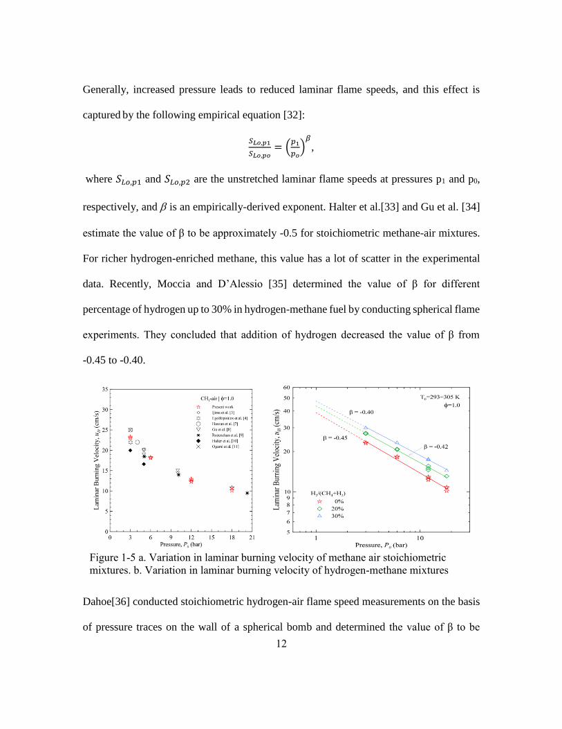
Figure 1-5 a. Variation in laminar burning velocity of methane air stoichiometric mixtures.
b. Variation in laminar burning velocity of hydrogen-methane mixtures ..... 12
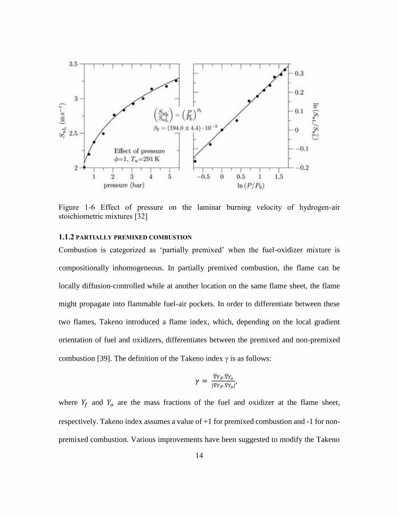
Figure 1-6 Effect of pressure on the laminar burning velocity of hydrogen-air
stoichiometric mixtures [32] .......................................................................... 14
Figure 1-7 Instantaneous velocity and scalar field at two instants of laminar flame
propagation at: (a) 1 ms, and (b) 4 ms after ignition. [44] (c) Turbulent stratified
flame propagation in a similar experimental set up [43] ............................... 17

xv
Figure 1-8: a. fully premixed laminar flame in the wake of a flameholder. [21] b. flame
profile in stratified laminar conditions c. Flame profile in turbulent stratified
conditions. [23] Blue arrow indicates the fuel-rich flow. .............................. 18
Figure 1-9: The classical model of boundary layer flashback (a) schematic of the flame
front with respect to the boundary layer, and (b) illustration of the critical
gradient model for three different velocity gradients. ................................... 19
Figure 1-10 Schematic showing the streamlines during flashback with a. no flame-flow
interaction b. strong flame flow interactions. Blue and red line represents the
flame profile and the approach flow streamlines respectively. ..................... 21
21
Figure 1-11: Simultaneous chemiluminescence images, particle images and velocity field
at the flame tip during flashback [45]. The straight line in the
chemiluminescence images show the location of laser sheet. ....................... 21
Figure 1-12: Different modes of flame flashback. (a) inside a channel or tube, (b) along the
axis of a vortex, and (c) along the walls of different geometry swirl combustors.
Blue line indicates the flame surface, while red arrow indicates the motion of
the flame tip. .................................................................................................. 23
Figure 1-13 Global propagation behavior of the flame tongue during methane air flashback.
a. Flame behind the center-body b. Flame tongue entering the front view c.
Flame bulges on the trailing edge are visible. Each of these instants are
separated by 10 milliseconds in time. Red arrow shows the direction of the
approach flow. Green arrow indicates the motion of the flame tongue. [56] 24
Figure 1-14: Streamlines in the unburnt gas region indicating the (a) reverse flow pockets,
and (b) flow deflection upstream of the flame tip. Streamlines are colored by
distance from the center-body. [53] ............................................................... 25

xvi
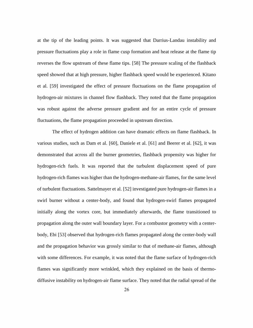
Figure 1-15 Chemiluminescence images of hydrogen-rich flame flashback as reported by
Ebi. Flame surface is highly wrinkled for hydrogen-rich flames, however the
global behavior of flame propagation remains the same as methane-air
flashback [53]. ............................................................................................... 27
Figure 2-1 The optically accessible swirl combustor. Swirl vanes and the fuel path is
illustrated in the inset. .................................................................................... 31
Figure 2-2 a. Cut out view of swirler showing the fuel path in red arrows b. Perspective
view of the swirler during the laminar flame test. One swirler vane and the
center-body is highlighted. ............................................................................ 34
Figure 2-3 Photograph of the elevated pressure chamber ................................................. 36
Figure 2-4 Section view of the pressure chamber showing the internal assembly ........... 37
Figure 2-5 Simplified Process and instrumentation diagram for the pressure chamber ... 40
Figure 2-6 a. Top view of the mixing tube showing the region occluded for luminosity
imaging. The position of the laser sheet and different regions of the field of
view are shown. b. Front view of the flame structure. .................................. 42
Figure 2-7 Schematic diagram of the field of view inside the mixing tube. A 266 nm sheet
is brought from the side of the mixing tube. .................................................. 44
Figure 2-8 (a) PLIF signal from the laser sheet after partially blocking the beam, and (b)
simultaneous laser sheet profile in the cuvette .............................................. 46
Figure 2-9 Typical shot-to-shot variation in 266 nm beam as measured from the cuvette
signal .............................................................................................................. 47
Figure 2-10 Background-corrected PLIF image for methane-air mixing at 3 atm, Reh =
18600. ............................................................................................................ 48
Figure 2-11 Optical diagnostic set up for elevated pressure experiments ........................ 51

xvii
Figure 2-12 Striated Mie scattering image captured at 3 atm and corresponding correlation
map (a) before sheet correction (b) after sheet correction ............................. 54
Figure 2-13 Flame edge detection on the basis of seeding particle density ...................... 55
Figure 2-14 Striated particle image during the elevated pressure flashback of methane-air
swirl flames .................................................................................................... 56
Figure 3-1 Schematic of the flame tongue propagation as viewed from the front and the
top. The blue line indicates the flame surface and the black arrows show the
approach flow pattern. The red arrow indicates the motion of the flame surface.
The green and pink rectangles show leading and trailing sides of the flame
tongue. ........................................................................................................... 58
Figure 3-2 Schematic of the flame topology..................................................................... 60
Figure 3-3 Definition of upstream locations ..................................................................... 61
Figure 3-4 Axial position of the flame tip during upstream propagation for a single
flashback event .............................................................................................. 63
Figure 3-5 a. Three instances of a flame tongue crossing the laser sheet b. Stacking of
planar flame profile to construct the flame surface ....................................... 64
Figure 3-6 a. Flame surface reconstruction b. Luminosity image for a methane-air swirling
flame flashback Reh = 6600 ........................................................................... 65
Figure 3-7 Comparison of the luminosity images and the projections from reconstructed
flame surface. Each frame is taken 1 millisecond apart. The trailing edge of the
flame tongue is not reconstructed. ................................................................. 67
Figure 3-8 The propagating flame tongue in a channel at two different instances. The red
line shows the flame and the arrow shows the direction of the streamlines. . 68
Figure 3-9 Divergence value distribution in the reconstructed flow field with a. only
unburnt gases b. unburnt, burnt and flame surface ........................................ 69

xviii
Figure 3-10 Isosurface plot of normalized divergence value of a. 0.4 and b. 0.6. Pockets of
high divergence are marked with a red circle ................................................ 70
Figure 3-11 Instantaneous quasi-streamlines in front of the flame surface. These
streamlines emanate in the boundary layer along the center-body ................ 72
Figure 3-12 Quasi-streamlines in flame’s frame of reference .......................................... 73
Figure 3-13 Isometric views of flame-flow interaction at the leading side of the flame
tongue in the lab and flame's frame of reference ........................................... 77
Figure 3-14 Wireframe representation of the flame surface(blue) and points of maximum
blockage effect (red dots) and a representative streamline ............................ 79
Figure 3-15 Representative quasi-streamline in flame's frame of reference. Free body
diagram illustrates the radial balance of forces, centrifugal (black) pressure
gradient (blue) and coriolis force (red) .......................................................... 81
Figure 3-16 Velocity components along the quasi-pathline. Red line indicates the location
of maximum divergence. ............................................................................... 82
Figure 3-17 Fictitious forces acting on the fluid parcel through representative pathline . 84
Figure 3-18 Variation of centrifugal term acting on the 100 different fluid particles after
the point of maximum blockage. ................................................................... 86
Figure 3-19 Variation in Coriolis force along 100 quasi-pathlines after the point of
maximum blockage ........................................................................................ 87
Figure 3-20 Radial acceleration along 100 different quasi-pathlines after point of maximum
blockage ......................................................................................................... 88
Figure 4-1 Different stages of stratified flames a. Stable in the combustor b. Stabilized in
mixing tube after flashback c. Flameholding ................................................ 91
Figure 4-2 Regime diagram marking the mode of upstream propagation. Red circle refers
to intermediate stabilization while the blue circle indicates flameholding. ... 93

xix
Figure 4-3 Two luminosity images captured 5 ms apart during the stratified flame flashback
of methane-air mixture. Reh = 6600. ............................................................. 95
Figure 4-4 Propagation of flame structure on the outer wall a. bright flame structure
appearance b. acute flame structure formation c. acute flame anchoring d.
upstream propagation towards flameholding. Red arrow shows the direction of
the approach flow. ......................................................................................... 97
Figure 4-5 Instantaneous PLIF snapshots showing the distribution of equivalence ratio at
flashback-equivalent conditions. Reh = 6600 .............................................. 100
Figure 4-6: Mean distribution of equivalence ratio during methane-air mixing at Reh =
6600, Global equivalence ratio = 0.63. ........................................................ 101
Figure 4-7 Luminosity image captured during methane-air stratified flame flashback a.
Gamma = 1 b. Gamma = 0.3 ....................................................................... 102
Figure 4-8 Chemiluminescence and the axial velocity fields at time instants: a. to, b. to +3,
c. to +4 and d. to +5 ms. Green line in the chemiluminescence images shows
the position of laser sheet. Evolution of a flame structure is marked by yellow
circle. ........................................................................................................... 104
Figure 4-9 Normalized acetone PLIF signal captured during the flashback .................. 106
Figure 4-10 Instantaneous equivalence ratio distribution during helium-air mixing Reh =
6300 ............................................................................................................. 108
Figure 4-11 Mean equivalence ratio distribution in the mixing tube. Reh = 6300 ......... 109
Figure 4-12 Chemiluminescence images and simultaneous axial velocity fields at different
time instances during flame propagation along the outer wall boundary layer.
White region in the velocity shows the burnt gas region. ............................ 111

xx
Figure 4-13 (a) Bright flame feature crossing the laser sheet and simultaneous 2D
divergence field, (b) Formation of acute tipped flame structure on the outer
wall .............................................................................................................. 114
Figure 4-14 Simultaneous luminosity images and 2D divergence maps. Regions of large
divergence correspond to the bright flame structures crossing the laser sheet.
..................................................................................................................... 116
Figure 4-15. Instantaneous PLIF images showing the small-scale fuel-rich structures in the
flow. These images correspond to methane-air flashback at 3 atm. Reh = 18600
ϕg = 0.85 ....................................................................................................... 117
Figure 4-16 Interaction of the flame surface and fuel-rich pockets in the approach flow.
(a) 1 atm, and (b) 3 atm. The orange ellipse mark the luminosity signal from
bright flame structures. The black ellipse shows corresponding effect on the
flame surface ................................................................................................ 118
Figure 4-17 Luminosity images captured during hydrogen-rich flashback at 3 atm a. to b.
to + 12 ms c. to + 14 ms; Reh = 18600 ϕg = 0.3 ......................................... 119
Table A-1 Flashback-critical equivalence ratios for premixed and stratified methane-
hydrogen swirl flames for different levels of hydrogen enrichment ........... 131
Figure C-1 Assembly of the central section of the pressure chamber ............................ 136
Figure C-2 Assembly of the upper section of the pressure chamber .............................. 137
Figure C-3 Assembly of the lower section of the pressure chamber .............................. 138
Figure D-1 Water-filling process of the pressure chamber. ............................................ 139
Figure D-2 Air supply and pressure monitoring at the top flange of the chamber ......... 140
Figure D-3 General arrangement of the set up during pressurized condition ................. 141

1
CHAPTER 1 : INTRODUCTION
Stringent emission restrictions on the power generation industry has led to a
renewed focus on clean energy research. One of the attractive ways to reduce the carbon
footprint of gas-turbine power plants is to blend hydrogen into the fuel [1]. However,
combustors designed for natural gas are not necessarily suitable for hydrogen-rich fuel
since the faster kinetics, lower density and higher diffusivity of hydrogen alter their
performance. Thus, accommodation of hydrogen-rich fuel in gas turbine power plants
necessitates combustor designs that can operate stably on fuels with variable composition.
The fuel flexibility of combustors is a challenging task since the dynamic properties of the
flame show significant variation with different percentages of hydrogen. The fuel
flexibility can also lead to problems such as flashback and blow off [2].
During flashback, an erstwhile stable flame propagates upstream into the mixing
tube, which may lead to the flame stabilizing inside the mixing tube; however, the mixing
tube components are usually not designed for high-temperature conditions and so may
become damaged by the presence of the flame. The resulting loss of mechanical integrity
could alter the combustor’s performance and efficiency. For high-hydrogen fuel air
premixtures, this situation can lead to potentially catastrophic conditions. Figure 1-1
illustrates the thermal damage incurred on the center-body of a combustor due to flashback
[3], [4].

2
Figure 1-1 a. Section view of the gas turbine combustor assembly. b. Swirlers and the
center-bodies in healthy condition c. Mechanical damage on the center-body due to
flashback. [4]
1.1 Literature Review
Flashback has been an active area of research for decades [5][6]. Most of the work
is relevant to industry needs and has focused on understanding flashback propensity and
its dependence on physical factors such as the tip temperature, swirl strength, geometry,
and hydrogen enrichment. In the last ten years, the focus of flashback research has shifted
toward understanding flame propagation using high-speed imaging, laser diagnostics and
numerical simulations. This thesis belongs to this line of research and hence we first review
the flame propagation mechanisms.
1.1.1 FLAME PROPAGATION
When the fuel and the oxidizer streams are well-mixed in a proportion such that it
would instantly ignite on providing some ignition source, the mixture is said to be
flammable. On the other hand, if the fuel or air is in excess such that no flame propagation
is achieved, the mixture is considered non-flammable. When the flame propagates through
a flammable mixture, it propagates like a wave that processes the unburnt reactants into
burnt products. Propagation behavior of such flames depend on several factors such as

3
combustion chemistry, strain rates, turbulence, ambient pressure, and temperature of the
reactants. In the next two subsections, we will review premixed flame propagation in
laminar and turbulent flows. We will also discuss how in certain flow configurations, such
as vortex flows, there might be faster propagation of the flame that cannot be modelled as
turbulent propagation.
1.1.1.1 Laminar premixed flame propagation
The laminar flame speed (SL) of a flammable fuel-air mixture is the speed with which a
flame would progress in a quiescent homogenous mixture under adiabatic conditions.
Under laminar, homogeneous, and one-dimensional conditions, the laminar flame speed
(SLo) of a planar flame front is governed by its thermo-chemical properties and hence
considered a function of the local equivalence ratio (ϕ). In general, flames are two- or three-
dimensional and are affected by flame-stretch (κ) [7], [8]. Flame stretch is defined as the
rate of change of surface area of a flame element per unit surface area, viz.,
𝜅 =1
𝐴
𝑑𝐴
𝑑𝑡
Conventionally, a flame is considered positively stretched for a spherically expanding
flame, and negatively stretched for Bunsen flames. The flame stretch may occur due to
aerodynamic effects, when the tangential and normal components of velocity stretch the
flame surface, or due to curvature of the flame sheet. For a stretched flame, imbalance in
convective and diffusive fluxes occur near flame surface; hence, flame stretch can have a
significant effect on the flame propagation speed when the fuel and air have different
molecular and thermal diffusivities. To quantify the relative role of these two factors, we
define Lewis number (Le=/D) as the ratio of thermal diffusivity () and mass diffusivity
4
(D). It has been found that for mixtures with Le < 1, the laminar flame speed increases with
positive stretch and vice versa. The effect of weak stretch (κ) on laminar flame speed is
quantified on the basis of the Markstein number (Ma) and unstretched flame thickness (δLo)
as follows:
𝑆𝐿,𝜅 = 𝑆𝐿,𝑜 − 𝜅 𝑀𝑎 𝛿𝐿𝑜,
where, SL,κ is the stretched flame speed while SL,o is the unstretched laminar flame speed.
[7]
1.1.1.2 Flame propagation along a vortex axis
Flame propagation along a vortex axis is relevant for swirling flames, especially
for flashback studies. These vortices can range from small scales, such as in tubular
combustors [9], to large scales, such as in weather cyclones [10]. It has been reported
widely by various researchers that the flame propagation in a vortical flow of fuel-air
premixture is faster along the axis, even under weak turbulence conditions [11]. This
characteristic also manifests itself into flashback in swirl combustors without center-body
[12], [13].
Flame propagation along a vortex exhibits higher flame speed along the axis than
in the transverse direction. This behavior has been found to exist for straight vortices (two
dimensional vortex structures) as well as for vortex rings (vortex structures whose axes are
closed curves in space) [14], [15]. The axial flame propagation speed has been found to
increase with the maximum azimuthal velocity in the vortex tube, and the density ratio
across the flame [11]. In addition, flame propagation along the vortex axis has also found
to sustain itself beyond the conventional flammability limits [16]. Figure 1-2 illustrates the

5
flame propagation along the axes of vortices withdifferent strengths. In the first case, the
flow inside a combustion chamber is kept still and a flame kernel was laser-ignited. The
flame kernel developedin spherical fashion. This case is illustrated in Figure 1-2(a), where
a flame kernel diameter grows to around 10 mm in 300 microseconds. In the other two
cases, the flame kernel was ignited in a vortical flow. In Figure 1-2(b), the flame structure
developing in a vortex flow, shows larger size in the axial direction of the vortex (y-axis in
the figure, ~ 15 mm). For stronger vortex, this propagation along the vortex axis was faster.
It should be noted that these vortices are two-dimensional in nature and the axial velocity
component is negligible. Hence, in vertical direction the propagation behavior should not
have changed. Though, it was noted that the flame propagates faster in vertical direction
[17]. The stronger vortex exhibited faster propagation of flame along its axis.
Figure 1-2 Schlieren images of hydrogen-nitrogen- mixture propagating in (a) non-swirling
flow, (b) vertical vortex of intermediate strength, and (c) vertical vortex with large strength.
The schematic shows the vortex axis and the growth of flame kernel in (c).

6
An explanation for this behavior is not feasible with one-dimensional picture as developed
in the previous subsection. The canonical 1D picture of the flame surface predicts a
pressure decrease across the flame due to the density decrease, whereas it has been
observed experimentally that the pressure across the vortex flame is higher on the burnt
gas side [16]. Researchers have postulated various models to explain the underlying
physics for such behavior of the flame surface. Of these, the vortex breakdown model by
Chomiak [18] and baroclinic vorticity generation mechanism proposed by Ashurst [19]
have generated immense interest. The baroclinic vorticity have been shown to play an
important role during the initial phase of propagation [16].
Swirling flame flashback, which occurs along a vortex core, is essentially a specific case
of flame propagation along the vortex axis. [20] Even when the flame propagates along the
boundary layer of the center-body in an annular combustor, it does so in a swirling
environment and factors such as baroclinic vorticity generation have been proposed as an
assisting factor for flame propagation [21]. It should be noted that turbulence plays little
role in such propagation, whereas aerodynamic factors such as azimuthal velocity have
been found to directly affect the flame propagation behavior [16].
1.1.1.3 Turbulent flame propagation
In most practical combustors the flame propagates in a turbulent flow environment.
Turbulent premixed flame propagation is generally studied as the movement of a highly-
wrinkled flame brush which propagates into the unburnt turbulent mixture [7]. Similar to
premixed-laminar flame propagation, where the flame is treated as a wave moving with the
laminar flame speed, turbulent-flame propagation is modeled as a wave that moves in space
7
with a characteristic velocity. To treat the flame brush as a wave, the motion of the mean
flame brush is used as the characteristic flame speed, also called the turbulent displacement
speed. The turbulent displacement speed of a flame brush is defined as follows,
𝑆𝑇,𝐷 = (𝑽𝒇 − 𝑽𝒈) ∙ �⃗� ,
where Vf and Vg are the average flame brush propagation speed and average unburnt gas
speed upstream of the flame, respectively. 𝑆𝑇,𝐷 refers to the turbulent displacement speed
of the flame brush. �⃗� refers to the mean flame brush normal unit verctor. Both velocity
vectors are measured in lab-frame. The turbulent displacement flame speed is difficult to
measure experimentally; hence, in several applications, an easily measurable quantity, the
fuel consumption speed is utilized. For turbulent flames, the global consumption speed
(𝑆𝑇,𝐺𝐶) is defined as follow:
𝑆𝑇,𝐺𝐶 =�̇�
𝜌𝐴𝑐=0.5
where �̇� is the mass flow rate, ρ is the density of the unburnt reactants, and 𝐴𝑐=0.5 is the
flame brush area corresponding to the mean reacted state. For an unstretched laminar flame,
the local fuel consumption speed is the same as the local flame displacement speed. It has
been found in various studies that turbulence enhances the flame speed significantly [7],
and this effect can be captured with the following relation,
𝑆𝑇
𝑆𝐿𝑜= 𝑓(
𝑢′
𝑆𝐿𝑜),
where 𝑢’ is the RMS of the velocity fluctuations. 𝑆𝑇 and 𝑆𝐿𝑜 is the turbulent flame speed
and unstretched laminar flame speed respectively. This definition has been found to have
substantial variation across different studies. It has been proposed that since the above

8
formulation doesn’t take flame stretch effects into account, it cannot capture the correct
physics of turbulent flame propagation [22].
Wrinkling of the flame surface can have dramatic effects on the flame propagation
behavior of fuel-air mixtures, especially with Lewis numbers less than unity [7]. Wrinkling
of the flame sheet modifies the thermal and diffusion processes, in ways that cannot be
accounted for in one-dimensional flame models. For example, convex flame tips (or
positively-stretched flames) have a larger supply of unburnt fuel species through diffusion,
whereas concave flame surfaces (negatively-stretched flames) have limited access to the
fuel. This difference results in higher flame speed at the flame tip and lower flame speed
(and possible local extinction) at the flame troughs. This thermo-diffusive effect is
generally stronger than the hydrodynamic instability and leads to cellular structure in lean
flames.
For lean fuel-air mixtures with Lewis number that is greater than unity, we have
the opposite behavior: flame tips with concave curved surfaces will have smaller flame
speed, while the concave features on the flame will have higher flame speed. This behavior
tends to stabilize the flame surface. For fuel-air mixtures with near unity Lewis numbers,
thermo-diffusive effects have only a small effect on the flame structure.
A modified expression for the turbulent flame speed is proposed by Driscoll [23]
where the geometry-dependent variation in turbulent speeds was taken into account by
including the integral length scale in the streamwise direction (𝑙 ):
𝑆𝑇
𝑆𝐿𝑜= 𝑓(
𝑢′
𝑆𝐿𝑜,𝛿𝐿𝑜
𝑙, 𝑀𝑎),
9
where 𝑢’ is the RMS of the velocity fluctuations. 𝑆𝑇 and 𝑆𝐿𝑜 is the turbulent flame speed
and unstretched laminar flame speed respectively. 𝛿𝐿𝑜 is the flame thickness of unstretched
laminar flame. Even after taking these factors in account, a strong quantitative scatter
exists among the turbulent speed measurements by various researchers, which suggests that
the geometry of the burner and the experimental set up might also have a role in turbulent
flame speed measurements. [23]
Recently, it has been suggested by Venkateswaran et al. [24] that for lean hydrogen-air
mixtures, the turbulent flame speed scales better with the maximum laminar stretched
flame speed, instead of the laminar flame speed. In their justification, they propose that
since the flame tip is generally richer than the rest of the flame sheet owing to the diffusion
of fuel species, it propagates at the maximum flame speed. They further argue that such
leading points dictate the global consumption speed of the turbulent flame brush.
1.1.1.4 Effect of hydrogen-enrichment on premixed flame propagation
Hydrogen enrichment of fuels is a well-established strategy to reduce the carbon footprint
of industrial burners. The addition of hydrogen to methane has been studied extensively by
previous researchers [25],[26]. These studies concluded that a linear increase in laminar
burning velocity is experienced upon the addition of hydrogen, up to the point when the
hydrogen content in the fuel is less than 0.7. For hydrogen content greater than 0.85, the
rate of increase in flame speed is much steeper. The reasoning for this behavior was
proposed that when hydrogen is the dominant fuel species, methane acts as an inhibitive
factor for hydrogen chemistry. Later, Di Sarli and Di Benedetto [27] utilized numerical

10
calculations to quantify three regimes in methane-hydrogen-air mixtures which they
described as methane-dominated combustion (H2 content less than 0.5), transition (H2
content from 0.5 to 0.9) and methane-inhibited combustion (H2 content 0.9 and above).
These regimes are illustrated in Figure 1-3. It should be noted that a linear interpolation of
the laminar flame speeds is not applicable to assess the increase in the laminar flame speed
in the transition regime.
Figure 1-3 Laminar burning velocity of hydrogen–methane/air mixtures as a function of
the hydrogen content at NTP conditions. Three regimes are defined for laminar flame speed
estimation. ϕ represents the equivalence ratio of the fuel-air mixture.
Hu et al. [28] determined the laminar burning velocity based on spherical-reactor
experiments for a range of hydrogen-percentages and equivalence ratios as shown in Figure
1-5. They concluded that for methane-inhibited flow regimes, the combustion is dominated

11
by H2 and OH radicals in the reaction zone which show faster chemistry as compared to
the methane-dominated regime. In their experiments, they also found the Markstein
number (defined in section 1.1.1.1) for a range of hydrogen-content and equivalence ratio.
It was shown that for the methane-inhibited regime, the Markstein number is either
negative or very close to zero. Wang et al. [29] reported that the effect of hydrogen addition
leads to less preference for aldehyde-dominated pathways, thereby reducing the aldehyde
emissions in methane combustion. A recent study by Qingfang et al. [30] showed that for
methane-rich fuel, CH3 consumption significantly adds to the global heat release, whereas
for hydrogen combustion, H and OH play the most important role.
Figure 1-4 Laminar flame speed of methane-hydrogen-air premixtures for different levels
of hydrogen enrichment: (a) 0-50%, and (b) 50-100%. X refers to the mole fraction. [31]
1.1.1.5 Effect of pressure on premixed flame propagation
Pressure influences flame propagation in different ways, but one of the most important is
that it directly affects the combustion kinetics and hence the laminar flame speed.
12
Generally, increased pressure leads to reduced laminar flame speeds, and this effect is
captured by the following empirical equation [32]:
𝑆𝐿𝑜,𝑝1
𝑆𝐿𝑜,𝑝𝑜= (
𝑝1
𝑝𝑜)𝛽
,
where 𝑆𝐿𝑜,𝑝1 and 𝑆𝐿𝑜,𝑝2 are the unstretched laminar flame speeds at pressures p1 and p0,
respectively, and is an empirically-derived exponent. Halter et al.[33] and Gu et al. [34]
estimate the value of β to be approximately -0.5 for stoichiometric methane-air mixtures.
For richer hydrogen-enriched methane, this value has a lot of scatter in the experimental
data. Recently, Moccia and D’Alessio [35] determined the value of β for different
percentage of hydrogen up to 30% in hydrogen-methane fuel by conducting spherical flame
experiments. They concluded that addition of hydrogen decreased the value of β from
-0.45 to -0.40.
Dahoe[36] conducted stoichiometric hydrogen-air flame speed measurements on the basis
of pressure traces on the wall of a spherical bomb and determined the value of β to be
Figure 1-5 a. Variation in laminar burning velocity of methane air stoichiometric
mixtures. b. Variation in laminar burning velocity of hydrogen-methane mixtures

13
0.194, which was smaller than the value 0.43, as found by Iijima and Takeno [37].
Recently, Salzano et al. [38] conducted burning velocity measurements for pressures up to
6 bar and concluded that the exponent β changes its sign from negative to positive for pure
hydrogen content..
Pressure also affects other flame characteristics. For example, the flame sheet
thickness tends to decrease with increasing pressure due to a decrease in thermal diffusivity
[7]. This thinning implies that there are sharper density gradients across the flame front at
elevated pressures. Increased density gradients across the flame front can lead to the
development of the Darrius-Landau instability, which is known to wrinkle the flame
surface. According to its definition, any planar flame across which density changes, is
intrinsically unstable, and with time, will develop positively and negatively curved surfaces
over entire flame sheet. In this instability, streamline divergence due to the thermal
expansion of unburnt gases upstream of the flame front causes a local deceleration of
unburnt gases in the vicinity of the flame surface. Owing to this, the flame starts
propagating faster in the lab frame of reference. On the other hand, if there is a streamline
convergence in front of the flame surface, flame propagation in the lab frame of reference
becomes smaller; thus, any initial perturbation grows with time, thereby wrinkling the
flame surface.
14
Figure 1-6 Effect of pressure on the laminar burning velocity of hydrogen-air
stoichiometric mixtures [32]
1.1.2 PARTIALLY PREMIXED COMBUSTION
Combustion is categorized as ‘partially premixed’ when the fuel-oxidizer mixture is
compositionally inhomogeneous. In partially premixed combustion, the flame can be
locally diffusion-controlled while at another location on the same flame sheet, the flame
might propagate into flammable fuel-air pockets. In order to differentiate between these
two flames, Takeno introduced a flame index, which, depending on the local gradient
orientation of fuel and oxidizers, differentiates between the premixed and non-premixed
combustion [39]. The definition of the Takeno index is as follows:
𝛾 = ∇⃗⃗ 𝑌𝐹.∇⃗⃗ 𝑌𝑜
|∇𝑌𝐹.∇𝑌𝑜|,
where 𝑌𝑓 and 𝑌𝑜 are the mass fractions of the fuel and oxidizer at the flame sheet,
respectively. Takeno index assumes a value of +1 for premixed combustion and -1 for non-
premixed combustion. Various improvements have been suggested to modify the Takeno
15
index to capture partially-premixed combustion characteristics. The measurement of flame
index in a reacting flow field provides important insight into the spatial distribution of heat
release and radical presence contributed by each type of combustion.
Da Cruz et al. [40] performed a numerical simulation of one-dimensional stratified
flame propagation in methane-air mixtures and found that the flame propagates faster when
it progresses from stoichiometric to lean premixtures. On the other hand, when the flame
progressed from stoichiometric to rich premixtures, it propagated at a slower speed. It was
argued that there is a memory effect and the flame propagation depends on the local
gradient of equivalence ratio. An enhanced population of H2 and CO radicals close to the
flame surface were thought to be responsible.
Bilger, in his well-cited paper [22], defined stratified combustion as the flame
propagation through inhomogeneous fuel air mixtures in which the stoichiometric fuel air
mixture doesn’t exist at any point in time and space. Lipatnikov follows the same definition
in his text book [8]. However, in a recent review paper by Masri [41], stratified combustion
has been defined as partially premixed combustion where the flame propagates in a
flammable mixture. No distinction for stoichiometric quantities was made in his review
paper. In our study, the definition by Masri [41] is followed.
Kang and Kyritsis [42] ran experiments with stratified methane-air mixtures and
found the flame propagation speed to be almost twice the laminar flame speed. In addition,
it was observed that the flame propagated in conventionally “non-flammable” fuel-air
mixtures. These results showed that the flame propagation through a stratified mixture
can’t be assumed to be quasi-homogenous and there indeed is a memory effect playing a
16
role in flame propagation. It was suggested that local flame propagation is not just a
function of local equivalence ratio (ϕ), but also the gradient of ϕ. In subsequent studies, to
define stratification, the alignment angle between the flame progress variable gradient and
the local equivalence ratio gradient is used to characterize stratified flames [41]. Stratified
flames were differentiated as back-supported vs. front-supported depending on whether the
flame is progressing from lean mixture towards the rich ones or the other way around. The
flame is said to be back-supported when the fuel-rich burnt gas has an excess of
combustion-critical radicals as compared to the unburnt gas. In this case, excess heat and
radicals would diffuse across the flame to the preheat zone and would assist in its
propagation. On the other hand, if the unburnt gas is richer than the burnt gas, there
wouldn’t be unidirectional movement of heat and excess radicals. In such a situation, flame
propagation may or may not be assisted by the stratification. In general, back-supported
flames have higher flame speeds, broader reaction zones and extended flammability limits.
Pasquier et al. [43] investigated the flame propagation through stratified propane-air
mixtures. In their work, the idea was to experimentally verify the memory effect proposed
by Cruz et al. [40]. To generate a stratified fuel-air mixture, an anisole-seeded fuel jet was
injected along the diameter of an optically accessible chamber. Jet and air flow rates were
maintained at constant flow rates to attain a statistically-steady turbulent flow. Ignition was
carried out at a fuel-rich location and the growth of the flame kernel was captured for a few
milliseconds using simultaneous PLIF and PIV, as shown in Figure 1-8(b). Based on the
flame propagation data conditioned on local equivalence ratio, it was found that when the
flame propagated from rich to stoichiometric mixtures, the local flame speed was higher.
17
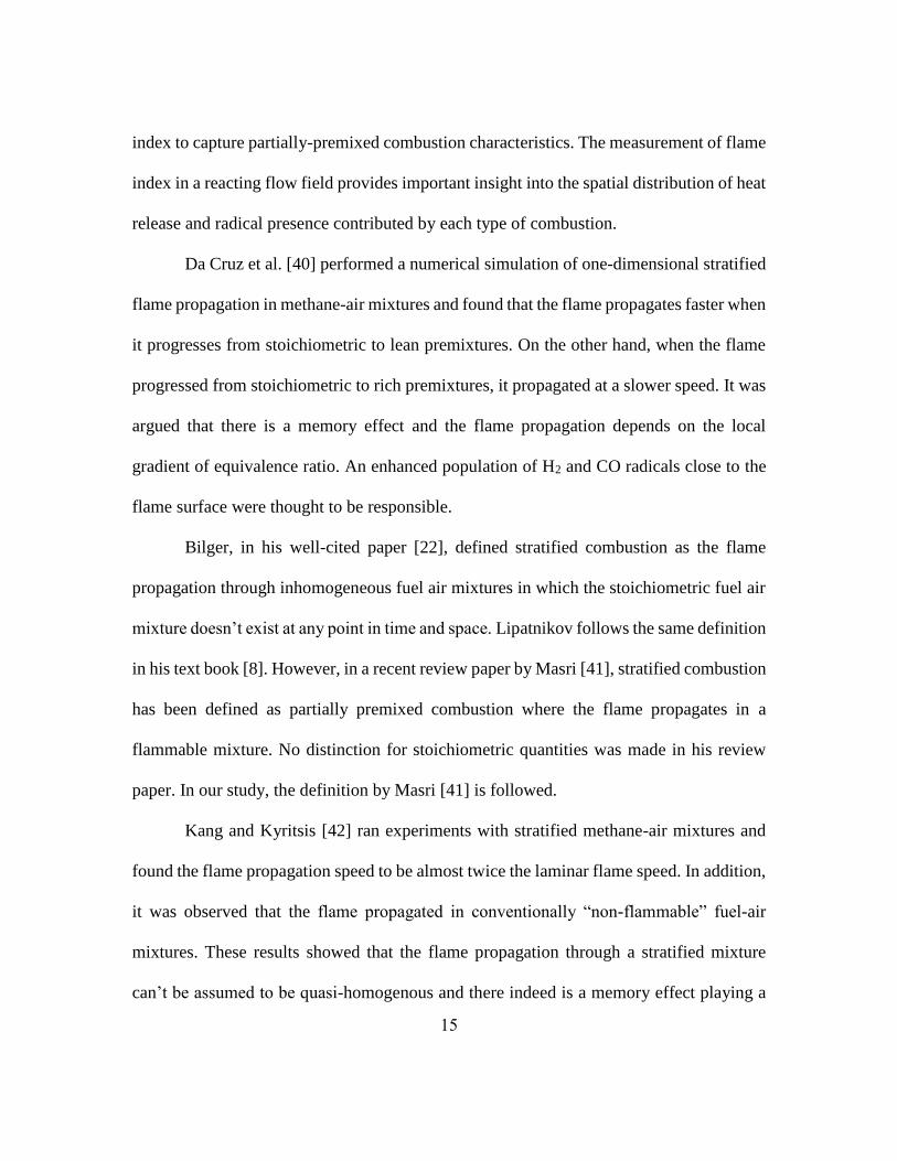
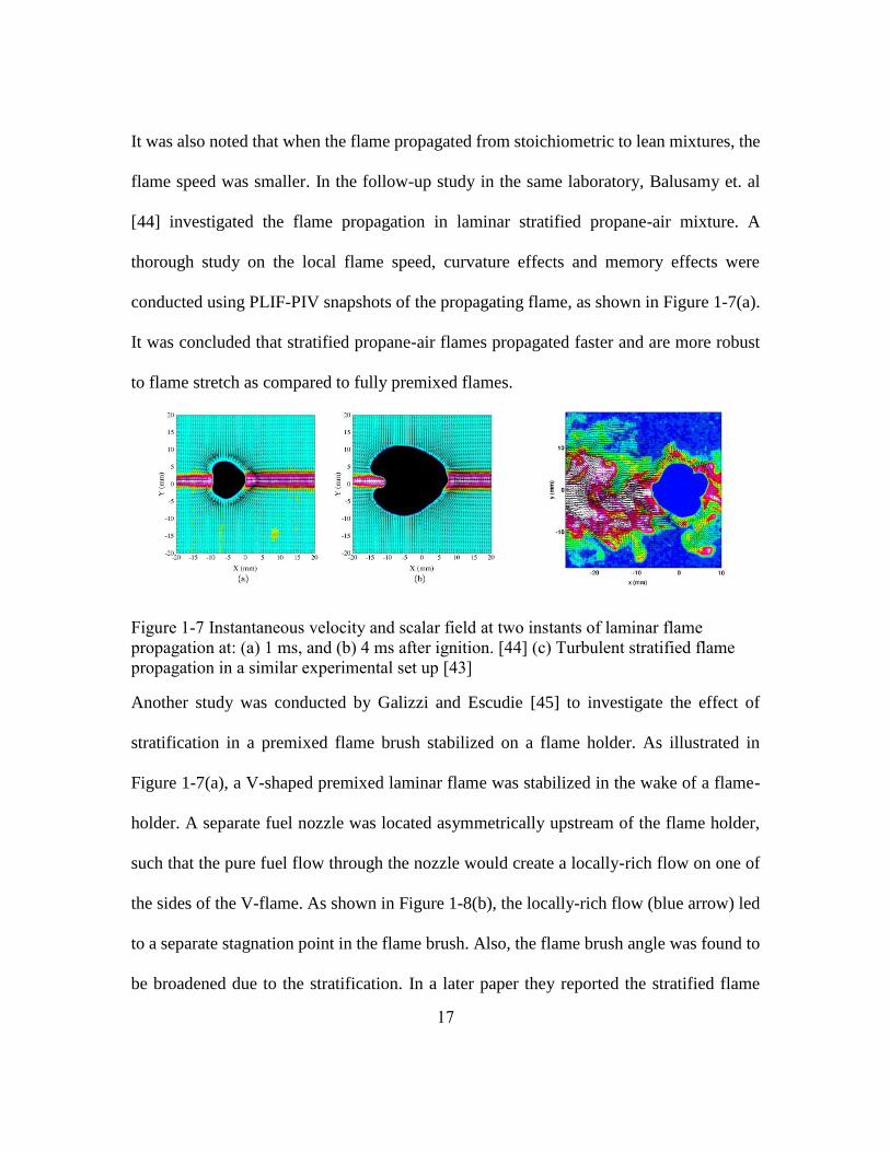
It was also noted that when the flame propagated from stoichiometric to lean mixtures, the
flame speed was smaller. In the follow-up study in the same laboratory, Balusamy et. al
[44] investigated the flame propagation in laminar stratified propane-air mixture. A
thorough study on the local flame speed, curvature effects and memory effects were
conducted using PLIF-PIV snapshots of the propagating flame, as shown in Figure 1-7(a).
It was concluded that stratified propane-air flames propagated faster and are more robust
to flame stretch as compared to fully premixed flames.
Figure 1-7 Instantaneous velocity and scalar field at two instants of laminar flame
propagation at: (a) 1 ms, and (b) 4 ms after ignition. [44] (c) Turbulent stratified flame
propagation in a similar experimental set up [43]
Another study was conducted by Galizzi and Escudie [45] to investigate the effect of
stratification in a premixed flame brush stabilized on a flame holder. As illustrated in
Figure 1-7(a), a V-shaped premixed laminar flame was stabilized in the wake of a flame-
holder. A separate fuel nozzle was located asymmetrically upstream of the flame holder,
such that the pure fuel flow through the nozzle would create a locally-rich flow on one of
the sides of the V-flame. As shown in Figure 1-8(b), the locally-rich flow (blue arrow) led
to a separate stagnation point in the flame brush. Also, the flame brush angle was found to
be broadened due to the stratification. In a later paper they reported the stratified flame
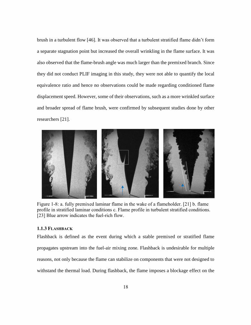
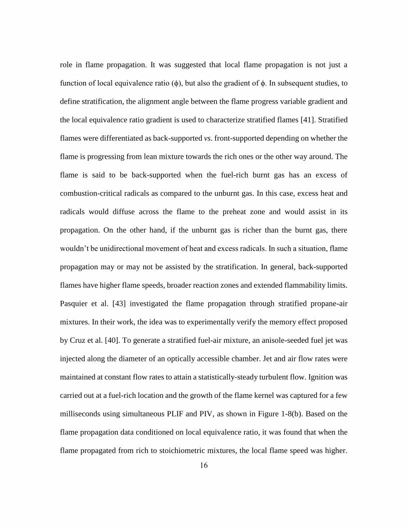
18
brush in a turbulent flow [46]. It was observed that a turbulent stratified flame didn’t form
a separate stagnation point but increased the overall wrinkling in the flame surface. It was
also observed that the flame-brush angle was much larger than the premixed branch. Since
they did not conduct PLIF imaging in this study, they were not able to quantify the local
equivalence ratio and hence no observations could be made regarding conditioned flame
displacement speed. However, some of their observations, such as a more wrinkled surface
and broader spread of flame brush, were confirmed by subsequent studies done by other
researchers [21].
Figure 1-8: a. fully premixed laminar flame in the wake of a flameholder. [21] b. flame
profile in stratified laminar conditions c. Flame profile in turbulent stratified conditions.
[23] Blue arrow indicates the fuel-rich flow.
1.1.3 FLASHBACK
Flashback is defined as the event during which a stable premixed or stratified flame
propagates upstream into the fuel-air mixing zone. Flashback is undesirable for multiple
reasons, not only because the flame can stabilize on components that were not designed to
withstand the thermal load. During flashback, the flame imposes a blockage effect on the

19
fuel-air flow, thereby changing the aerodynamics in the combustion chamber. This can lead
to acoustic disturbances in the system that may trigger combustion instabilities. In addition,
the flame-wall interaction not only reduces the availability of thermal energy for gas
turbines but also increases the presence of unburnt radicals. The combustion research
community has tried to understand the flashback physics and ways to avoid it, with limited
success. In this subsection, we will first discuss the flashback in simple non-swirling flows.
We will further consider how swirl affects flame propagation and then the effect of fuel-
air stratification on flashback.
1.1.2.1 Flashback in non-swirling flows
Examples of flashback in non-swirling flows include flashback in a channel flow or a
Bunsen burner. In both of these cases, flashback has been found to occur along the
boundary layer at the wall of the pipe or channel. The classical model on flashback was
proposed by Lewis and von Elbe [5].
Figure 1-9: The classical model of boundary layer flashback (a) schematic of the flame
front with respect to the boundary layer, and (b) illustration of the critical gradient model
for three different velocity gradients.

20
Figure 1-9(a) shows a schematic that illustrates the critical gradient model. The flame
(shown in red) propagates upstream through the low stream-wise momentum zone in the
boundary layer. The flame tip is located at a location δp (penetration length) away from
the wall. Owing to the heat loss to the wall, flame can exist only above δq (quenching
distance) from the wall. Figure 1-9(b) shows three cases of velocity gradient close to the
wall. The red line in this plot shows the component of flame propagation velocity in the
stream-wise direction. When the velocity gradient is smaller than the critical velocity
gradient gc, the flame speed at the penetration length is larger than the approach flow speed,
and hence the flame would propagate upstream. This classical model provides a standard
metric for flashback to occur; however, the critical-gradient model is overly simplistic as
it fails to describe the correct flame propagation speed [47]. The main problem is that the
critical gradient model assumes that the incoming flow stays isothermal even in the vicinity
of the flame; however, the flame substantially alters the incoming flow and leads to
significant streamline divergence at the flame front [48]. Figure 1-10(a) shows the
schematics for cases with and without flame flow interactions. The red and blue lines show
the approach flow streamlines and flame surface respectively. When the flame and the flow
do not interact, the streamlines stay straight while passing through the flame surface. This
situation is easier to model and would be true for a situation when the density change across
the flame surface is assumed to be negligible. On the other hand, when the volumetric flow
generation across the flame surface is taken into account, the upstream approach flow
streamlines diverge prior to entering the flame. This situation is illustrated in the Fig 1-
10(b).
21
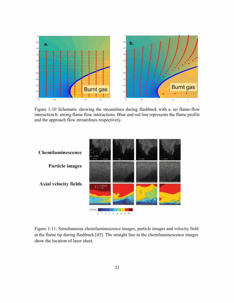
Figure 1-10 Schematic showing the streamlines during flashback with a. no flame-flow
interaction b. strong flame flow interactions. Blue and red line represents the flame profile
and the approach flow streamlines respectively.
Figure 1-11: Simultaneous chemiluminescence images, particle images and velocity field
at the flame tip during flashback [45]. The straight line in the chemiluminescence images
show the location of laser sheet.
a. b.
22
At TU Munich, Eichler et al. [49] and Baumgartner [50] investigated turbulent flame
propagation along a flat wall. It was observed that the flame propagation was led by small
“bulges” or “tips,” where the flow field upstream of it exhibited reversal of flow. This
region is shown in blue in axial velocity maps in Figure 1-11. Baumgartner [50], in his
thesis, proposed that the flame structures impose an adverse pressure gradient on the
incoming flow, there inducing the separation of boundary layer. Hoferichter et al. [51] tried
to model the flashback on the basis of the adverse pressure gradient imposed by the flame
front.
1.1.2.2 Flashback in swirling flows
Flashback in gas turbine combustors may assume different modes of upstream propagation
depending on the flow geometry. It might occur along the wall boundary layer [52], along
the vortex core [12] or along the center-body boundary layer [53], as shown in Figure 1-
11. Flame propagation along the vortex core happens even though the bulk flow velocity
is much larger than the flame speed. Konle and Sattelmayer [54] proposed the role of
combustion-induced-vortex-breakdown (CIVB) in assisting the flame propagation through
core of swirling flows.
23
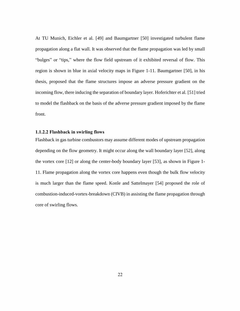
Figure 1-12: Different modes of flame flashback. (a) inside a channel or tube, (b) along
the axis of a vortex, and (c) along the walls of different geometry swirl combustors. Blue
line indicates the flame surface, while red arrow indicates the motion of the flame tip.
They suggested that since at the flame sheet, pressure gradient and the density gradients
are misaligned, the resulting baroclinic torque supports the vortex breakdown at the tip of
the flame. Negative azimuthal vorticity production at the tip leads to vortex breakdown
which furthers the propagation of the flame. Numerical results obtained using unsteady
RANS were found to support this proposition [20]; however, no experimental work has
established the existence of a stagnation point upstream of the flame tip in a vortex core.
At TU Darmstadt, Heeger et al. [21] investigated lean-premixed swirl flame flashback and
observed a negative axial velocity field upstream of the flame tip, which propagated along
the center-body boundary layer. It was assumed then that these negative-axial velocity
regions are akin to the one observed by Eichler et al. [49]. It was concluded that the flame
tip separates the boundary layer upstream of it and thus its propagation gets assisted by the
reversal of flow. However, in their study, there were no provisions to measure the out-of-
24
plane velocity component which, as shown later, might have important implications in
swirl flows.
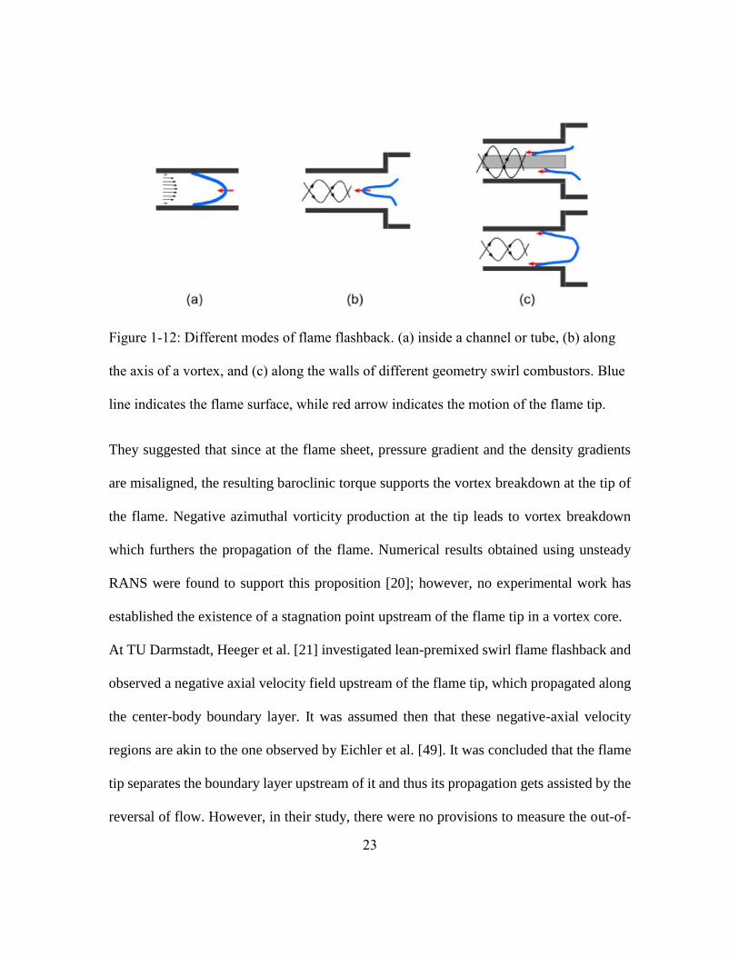
Ebi and Clemens [55] studied premixed flame flashback in a swirl-flame combustor
with premix tube with center-body. They used time-resolved tomographic PIV
measurements to examine the flow in proximity of the flame tip. They observed a negative
axial velocity region, akin to the findings of Eichler et al. [49], was present on the side of
the large flame tongue, which propagated along the center-body boundary layer. The global
flame propagation behavior is illustrated in Figure 1-13. The flame tongue swirls around
the center-body in the same fashion as the approach flow. The axially upstream motion of
the flame is led by the flame tip. Behind the flame tip region is the trailing edge of the
flame brush. This region is marked by the presence of the small flame bulges. The flame
propagation was found to occur over a few milliseconds and the temperature of the center-
body (less than 100˚C in their case) was not found to affect this behavior.
Figure 1-13 Global propagation behavior of the flame tongue during methane air flashback.
a. Flame behind the center-body b. Flame tongue entering the front view c. Flame bulges
on the trailing edge are visible. Each of these instants are separated by 10 milliseconds in
time. Red arrow shows the direction of the approach flow. Green arrow indicates the
motion of the flame tongue. [56]

25
However, their three-component PIV measurements showed that the negative axial
velocity region was associated with flow deflection rather than flow reversal. This
observation ruled out the leading role of boundary layer separation in flame propagation in
lean-premixed swirl flame flashback. In Figure 1-14, instantaneous streamlines
approaching the flame tongue from different locations, are shown. In the first case, the
streamlines were found to reverse near the flame bulge. Near the leading edge of the flame,
the flow was found to deflect in the direction of the swirl. These effects are illustrated in
Figure 1-13. The streamlines approaching the flame and the pockets of flow upstream of
the flame bulge are directed in opposite direction (actual reversal), as shown in Figure 1-
13(a). The deflection of streamlines in Fig 1-13(b) can be observed as bending of
streamlines (notice green streamlines in comparison with red streamlines).
Figure 1-14: Streamlines in the unburnt gas region indicating the (a) reverse flow pockets,
and (b) flow deflection upstream of the flame tip. Streamlines are colored by distance from
the center-body. [53]
A recent DNS study by Gruber et. al [57] investigated premixed hydrogen-air
flashback in a channel flow and observed the regions of negative stream-wise velocity form
26
at the tip of the leading points. It was suggested that Darrius-Landau instability and
pressure fluctuations play a role in flame cusp formation and heat release at the flame tip
reverses the flow upstream of these flame tips. [58] The pressure scaling of the flashback
speed showed that at high pressure, higher flashback speed would be experienced. Kitano
et al. [59] investigated the effect of pressure fluctuations on the flame propagation of
hydrogen-air mixtures in channel flow flashback. They noted that the flame propagation
was robust against the adverse pressure gradient and for an entire cycle of pressure
fluctuations, the flame propagation proceeded in upstream direction.
The effect of hydrogen addition can have dramatic effects on flame flashback. In
various studies, such as Dam et al. [60], Daniele et al. [61] and Beerer et al. [62], it was
demonstrated that across all the burner geometries, flashback propensity was higher for
hydrogen-rich fuels. It was reported that the turbulent displacement speed of pure
hydrogen-rich flames was higher than the hydrogen-methane-air flames, for the same level
of turbulent fluctuations. Sattelmayer et al. [52] investigated pure hydrogen-air flames in a
swirl burner without a center-body, and found that hydrogen-swirl flames propagated
initially along the vortex core, but immediately afterwards, the flame transitioned to
propagation along the outer wall boundary layer. For a combustor geometry with a center-
body, Ebi [53] observed that hydrogen-rich flames propagated along the center-body wall
and the propagation behavior was grossly similar to that of methane-air flames, although
with some differences. For example, it was noted that the flame surface of hydrogen-rich
flames was significantly more wrinkled, which they explained on the basis of thermo-
diffusive instability on hydrogen-air flame surface. They noted that the radial spread of the
27
propagating flame skirt was smaller than for the methane-air flames, as shown in Figure 1-
15.
Figure 1-15 Chemiluminescence images of hydrogen-rich flame flashback as reported by
Ebi. Flame surface is highly wrinkled for hydrogen-rich flames, however the global
behavior of flame propagation remains the same as methane-air flashback [53].
Sayad et al. [13] observed that for preheated hydrogen-methane-air mixtures,
flashback might occur by autoignition. Autoignition generally occurs when the residence
time of the fuel-air mixtures is larger than the ignition delay of the fuel-air mixtures. Beerer
and McDonell [63] in their attempt to measure the ignition delay of hydrogen-air mixtures
in gas turbines, found that the temperature at the premixing tube wall was high, even though
auto-ignition had not occurred. It was supposed that the flow in the boundary layer has
larger residence time, hence auto-ignition might have occurred along the wall. Another
possibility was suggested to be the catalytic effects for the surface itself.
There have been few experimental studies that have focused on flashback under
elevated pressure conditions [62],[64],[65],[66],[67]. Only one of these studies, by Mayer
et al. [65], has observed the behavior of upstream propagation of hydrogen-air flames at
28
elevated pressure using time-resolved laser diagnostics. In their study, it was noted that for
hydrogen-air flames, the flashback propensity increased with pressure and the critical
gradient was found to be an order of magnitude higher than the atmospheric pressure cases.
The critical gradients predicted by Fine [68] for sub-atmospheric pressure flashback were
not found to be applicable. It was noted that the flashback prediction models for
atmospheric pressure experiments may not be applicable at elevated pressure.
1.1.2.3 Flashback in partially-premixed fuel-air mixtures
Partial premixing of fuel-air mixtures has been a popular strategy to avoid flashback
in industrial combustors. By partial premixing of fuel, regions prone to flashback such as
vortex core or wall boundary layer can be kept too lean for flame propagation. However,
depending on whether the flame is back-supported or front-supported, the flammability
limits of the fuel-air mixture may be very different from conventional flammability limits
[41]. This brings in the necessity to understand flame propagation in stratified mixtures.
So far, there are two studies on flashback in a partially-premixed fuel-air mixtures. A joint
experimental and numerical study by Sommerer et al. [69] involved studying the flashback
in propane-air premixtures at atmospheric pressure. High-speed OH luminescence was
captured at 10 kHz during flashback. It was noted that the flame flashed back along the
vortex core of the swirl flames. For the analysis of numerical results, a modified flame
index was utilized to predict the percentage of premixed and non-premixed flames in the
flame brush. It was noted that upon flashback, the flame stabilized on the lip of the fuel
injector and thus, the fraction of non-premixed flames increased by a factor of three.

29
Another study which reported flashback in a hydrogen-air partially premixed
mixture was carried out at TU Munich. Utschick and Sattelmayer [70] investigated the
possibility of sustained flashback that leads to flame-holding on the injection ports. Partial
premixing of fuel was done by injecting the hydrogen-fuel through two types of injectors,
one which injected the fuel normal to the flow, another which injected fuel iso-kinetically
into the system. Ignition was triggered into the fuel-air mixing tube by laser ignition. A set
of experimental conditions were mapped out for the flame-holding to occur. Based on flow
conditions, a Damkohler number criteria was defined for which the flame-holding could
not happen in the mixing tube. In another study by Utschick et al. [71], flame propagation
behavior in the mixing tube was studied. By employing high-speed stereoscopic OH-
luminescence imaging, it was noted that the flame moved along the outer wall on a helical
path until it stabilized on the fuel ports.
1.2 Context of current work
As evident in the existing literature, flashback is a complex multi-physics process
that requires further study, especially for swirling flows. In this study we aim to improve
knowledge of flashback physics by investigating the flow near the leading side of the flame
surface. The details of the flame-flow interaction are investigated using high-speed
luminosity imaging and simultaneous particle image velocimetry. We have two main
objectives in this study.
The first is to develop an improved understanding of the propagating swirl flame
under fully-premixed conditions and to analyze its role in flashback assistance. For this
purpose, a new analysis technique is applied that enables the three-dimensional structure
of the flow to be reconstructed. The analysis from the flame frame-of-reference reveals the

30
role of inertial forces in the swirling-flame-flow interaction. A fundamental picture of
azimuthal propagation of the flame is developed.
The second objective of this study is to understand the effect of fuel-air
stratification on the flame propagation behavior. We induce stratification in the radial
direction by placing the fuel injection ports on the radially outward section of the swirl
vanes. The equivalence ratio field is analyzed to characterize the nature of the stratification
in non-reacting flow. Further, we conduct reacting flow experiments and report different
propagation behavior of flashback and the role of hydrogen-enrichment on flashback
behavior. The global behavior of upstream propagation is studied for pressures up to 5 atm.
However, laser diagnostic experiments are carried out up to 3 atm. Laser diagnostic
experiments are used to reveal the role of equivalence ratio inhomogeneities on flame
propagation behavior.
In the end, we discuss a general picture of flame-flow interactions on the upstream
propagation of the flame inside the mixing tube. The limitations of the current study and
possible research directions to further our understanding of flashback is explored.

31
CHAPTER 2 : EXPERIMENTAL SET UP
The flashback experiments were conducted with an annular swirl combustor which
was mounted inside an elevated pressure chamber. A set of high-speed cameras and lasers
were used to observe the flame propagation. In this section, we describe these experimental
set ups in detail.
2.1 Swirl Combustor
The swirl combustor assembly used in these experiments is a lab-scale prototype of
industrial combustors as shown in Figure 2-1. The section view of the combustor is
illustrated below:
Figure 2-1 The optically accessible swirl combustor. Swirl vanes and the fuel path is
illustrated in the inset.
It can be divided into three main sections: the plenum, the mixing tube, and the
combustion chamber. The main air flow through the combustor enters the annular plenum

32
region through four inlet ports, positioned symmetrically around combustor center-line.
Entry of air through these ports is depicted in Figure 2-1. Afterwards, this flow gets
conditioned by passing through annular honeycomb straighteners and two stations of fine-
wire mesh. The flow then passes through the swirl vane and into the mixing tube. The
mixing tube consists of a center-body and an outer cylindrical wall. The axial swirler is a
prototype of an industrial swirler with an inner and outer diameter of 25.4 and 50.8 mm
respectively. The swirler body is made with cobalt-chrome and was three-dimensionally
printed with an uncertainty of ±60 microns. It was equipped with eight symmetric
aerodynamically-curved vanes. Each swirler vane was angled at 60 degrees with respect to
the combustor axis. These vanes were also equipped with fuel injection ports for use in
partially-premixed flashback experiments. The fuel-entry paths through these ports are
different than the main air flow and shall be discussed in a subsequent paragraph. The axial
swirler imparts large azimuthal momentum to the approach flow. Numerical simulations
of the flow at the exit of the mixing tube indicated that the swirl number is 0.9. The swirl
number is the ratio of azimuthal to axial momentum flux of the swirling flow. The near-
unity swirl number indicates that the flow in the mixing tube is of high swirl, according to
conventional definitions (Swirl number > 0.6). The center-body of the mixing tube is
attached coaxially to the downstream end of the axial swirler. The center-body is a lathe-
machined stainless-steel cylinder with an outer diameter of 25.4 mm. Prior to installation,
the near-polish-finished center-body surface was painted with an ultra-flat black spray
paint (Krylon 5BIEP), which was desired to minimize the reflected light signal off the
center-body. The outer wall of the mixing tube was made of optical grade fused silica
(Heraeus Suprasil 310), which allowed optical accessibility into the flow field upstream of
the combustion chamber. The inner diameter of the outer wall was 52 mm. The annular
space of the mixing tube was bounded by the center-body and the inner wall of the fused
33
silica tube. To ensure that the fused silica tube could be mounted co-axially with the center-
body, a specially-designed alignment apparatus and screw-tightening methodology was
used. Downstream of the annular mixing tube, the flow opened up into the combustion
chamber that had nearly twice the outer diameter of the mixing tube. The center-body end
plane was flush with the mixing tube exit plane. The inner diameter of the combustion
chamber was 100 mm and its axial length was 150 mm. The combustion chamber and
mixing tube were held fixed by sandwiching these components between the holding plate
at the top and the plenum plate, as shown in the Figure 2-1 The glass-metal components
were sealed by using 1/8” thick ceramic paper gaskets (custom cut, in-house), which could
withstand temperatures in up to 1200˚C. Additionally, the padding provided by these
gaskets compensated for the thermal expansion mismatch between the steel and the glass.
The fuel streams through the swirl-vane injection ports follow a different flow-path
prior to entering the mixing tube. The central space in the plenum was occupied by a hollow
tube that was connected to the swirler and the center-body. The hollow tube was connected
to a fuel line, independent of the main swirl flow lines. The inner regions of the swirler and
the center-body were also designed to be hollow, thereby providing continuous access to
the swirler vanes and the center-body. This access to the center-body was used to route
thermocouples, which were used to measure the temperature of the center-body during
flashback. Fuel was passed through internal passages in the swirl vanes and then injected
into the main flow. The passages were cylindrical in shape and 3 mm in diameter. The fuel
injection ports in the swirl vanes were 1 mm in diameter. Two ports were used on each
vane. These fuel ports injected the fuel normal to the swirl vane surface, akin to a JICF
(jets-in-crossflow) configuration. These ports were located at a radial position 3 mm away
from the outer wall to introduce mean radial stratification in the mixing tube. It should be

34
noted that this inner-fuel-flow-design was optimized by doing several iterations of 3D
printed plastic swirlers. Thin-channel designs are prone to be asymmetric due to large
relative machining error (6-10%) and the possibility of partial choking of flow paths due
to contaminants in the flow line. To minimize such problems, all of the flow paths were
kept straight (easy-to-clean) and orthogonal at branching nodes (easy to ensure symmetry).
As a qualitative way to ensure symmetric behavior across all flow passages, a laminar
diffusion-flame test was developed, as shown in Figure 2-2(b).
a. b.
Figure 2-2 a. Cut out view of swirler showing the fuel path in red arrows b. Perspective
view of the swirler during the laminar flame test. One swirler vane and the center-body is
highlighted.
In this laminar-flame test procedure, a very small amount of fuel was continuously
flown through the swirler vanes. Thereafter, diffusion flames were ignited in a fashion like
a kitchen-stove burner. The resulting flame pattern indicated the symmetric nature (or the
lack of it) of the flow through the injection ports. Any loss of symmetry indicated a possible
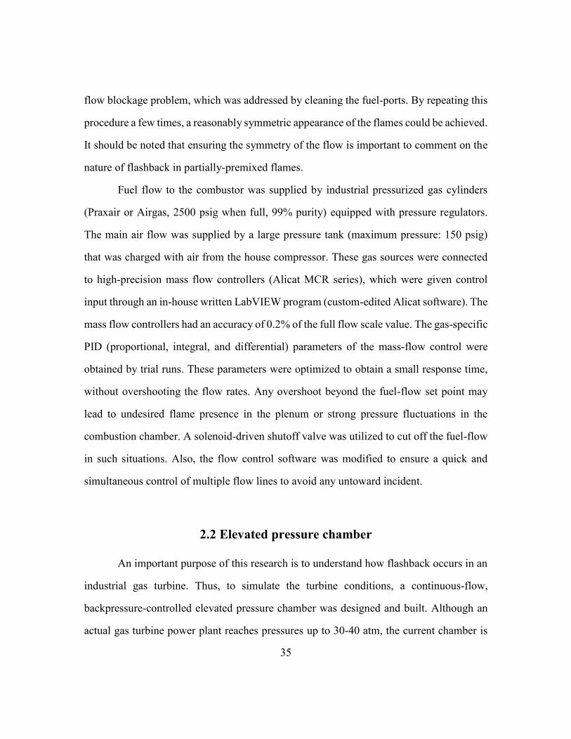
35
flow blockage problem, which was addressed by cleaning the fuel-ports. By repeating this
procedure a few times, a reasonably symmetric appearance of the flames could be achieved.
It should be noted that ensuring the symmetry of the flow is important to comment on the
nature of flashback in partially-premixed flames.
Fuel flow to the combustor was supplied by industrial pressurized gas cylinders
(Praxair or Airgas, 2500 psig when full, 99% purity) equipped with pressure regulators.
The main air flow was supplied by a large pressure tank (maximum pressure: 150 psig)
that was charged with air from the house compressor. These gas sources were connected
to high-precision mass flow controllers (Alicat MCR series), which were given control
input through an in-house written LabVIEW program (custom-edited Alicat software). The
mass flow controllers had an accuracy of 0.2% of the full flow scale value. The gas-specific
PID (proportional, integral, and differential) parameters of the mass-flow control were
obtained by trial runs. These parameters were optimized to obtain a small response time,
without overshooting the flow rates. Any overshoot beyond the fuel-flow set point may
lead to undesired flame presence in the plenum or strong pressure fluctuations in the
combustion chamber. A solenoid-driven shutoff valve was utilized to cut off the fuel-flow
in such situations. Also, the flow control software was modified to ensure a quick and
simultaneous control of multiple flow lines to avoid any untoward incident.
2.2 Elevated pressure chamber
An important purpose of this research is to understand how flashback occurs in an
industrial gas turbine. Thus, to simulate the turbine conditions, a continuous-flow,
backpressure-controlled elevated pressure chamber was designed and built. Although an
actual gas turbine power plant reaches pressures up to 30-40 atm, the current chamber is
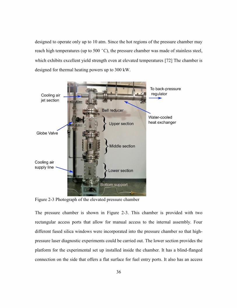
36
designed to operate only up to 10 atm. Since the hot regions of the pressure chamber may
reach high temperatures (up to 500 ˚C), the pressure chamber was made of stainless steel,
which exhibits excellent yield strength even at elevated temperatures [72] The chamber is
designed for thermal heating powers up to 300 kW.
Figure 2-3 Photograph of the elevated pressure chamber
The pressure chamber is shown in Figure 2-3. This chamber is provided with two
rectangular access ports that allow for manual access to the internal assembly. Four
different fused silica windows were incorporated into the pressure chamber so that high-
pressure laser diagnostic experiments could be carried out. The lower section provides the
platform for the experimental set up installed inside the chamber. It has a blind-flanged
connection on the side that offers a flat surface for fuel entry ports. It also has an access

37
door on opposite side that is useful for the installation and adjustment of the internal
assembly. The inlet for the cooling air co-flow is provided at the center of the bottom face.
The inlet of cool air co-flow is shown in the cut-out image of the pressure chamber in
Figure 2-4.
Figure 2-4 Section view of the pressure chamber showing the internal assembly
The middle section consists of three rectangular windows, two large ones (6” × 2.4”) and
a smaller one (4” ×1.5”), to allow optical access to the test section. The axes of the larger
windows are at an angle of 70 deg with respect to the smaller window in the horizontal
plane. The orientation of the large windows allows for stereoscopic PIV to be conducted.
The windows are made of S1UV fused silica glass (supplied by Esco Optics), which have
high transmission for UV light.

38
The upper section features another access port, which was primarily used to install the
calibration target for stereo PIV. Attached to the upper section is a bell reducer, which acts
as a passage for the hot exhaust gases. The smooth transition from 8-inch diameter to 4-
inch diameter piping allows for streamlined flow of the cooling air. This geometry
maintains low acoustic noise in the chamber, which is necessary for safe operation. At the
top of the chamber, another window is provided to allow for a laser sheet to enter the
chamber. To shield this window from hot gases, additional cooling air is supplied from the
side that reroutes the exhaust and decreases the sudden rise in temperature at the glass
surface. A thin sacrificial glass plate is provided in the window assembly to protect the
main window from the hot gases. The high-pressure chamber is versatile in the sense that
it can host various combustor geometries. Air mass flow rates to the combustor of up to
0.1 kg/sec are possible, which corresponds to a Reynolds number of 200,000 at 150 psi
based on the tube diameter of 50 mm. The chamber is designed for thermal heating powers
up to 300 kW. The vertical pipe assembly offers great adaptability for different
visualization methods. Depending on optical access requirements, the middle section can
be replaced to allow alternate window locations. The top window is ideal to observe the
flashback process in a transverse plane.
Safety has been given utmost importance in designing of this pressure chamber.
The glass windows have been designed with a high safety factor ( ̴10). A pressure safety
valve is provided in the bottom section of chamber. The cooling air supply tank is kept at
the maximum of 150 psi which is also the maximum design pressure of the chamber. Thus,
during operation, the pressure chamber is inherently safe against any unintended rise in
airflow.

39
2.2.1 FLOW THROUGH THE PRESSURE CHAMBER
Fig 2-5 shows a simplified process and instrumentation diagram for the pressure
chamber. The cooling air is supplied to the pressure chamber from a medium pressure gas
tank (maximum pressure 150 psi) located at the Wind tunnel lab, Pickle Research Campus.
The flow through the supply line is controlled using a control valve that is normally-closed
and is provided a diaphragm actuator pressure of 40 psi. A set of ball valves are included
in the air supply line to isolate different sections of the process flow during start up. Fuel
is supplied to the set up through industrial gas cylinders equipped with standard gas
pressure regulators. A bank of high-precision mass flow controllers (Alicat scientific, ±
0.2% full scale accuracy) are used to supply the air and fuel flow through the combustor.
The cooling air co-flow is regulated using the globe valve (typical opening of a quarter
turn) and the control valve. The cooling air supply line (diameter 2 inch) opens at the
bottom flange of the pressure chamber. The cooling air jet spreads out in the pressure
chamber (inner diameter of 8 inches) and flows around the internal assembly of the
combustor. Upon crossing the combustor’s location, the cooling air shrouds the inner walls
of the pressure chamber and gradually mixes with the combustion products of the swirling
flame.

40
Figure 2-5 Simplified Process and instrumentation diagram for the pressure chamber
The entire pressure chamber facility was operated remotely from a control station
equipped with four different computer systems. These computer systems were remotely
connected on the internal network to the master computers for processes such as image
capturing and pressure chamber monitoring. In addition to the cameras for optical
diagnostics, a set of security cameras were installed to monitor the experimental facility
area during the experiments.
2.3 Optical diagnostics
2.3.1 CHEMILUMINESCENCE IMAGING
High-speed chemiluminescence imaging was used extensively to investigate
flashback. For this purpose, a high-speed imaging camera (Photron APX) with a mounted
external intensifier (HiCatt, Lambert Instruments) is used to capture the flame propagation.

41
Depending on the experimental requirements, a 105mm Nikon lens (narrow view) or 70-
250 Tokina lens (wider view) is used. Typically, luminosity images are captured at 4 kHz
with an exposure of 250 microseconds. The intensifier gate is kept at 50 and 100
microseconds for methane-air and hydrogen-rich flames, respectively. For corresponding
cases, the intensifier gain is kept at 750 and 850. During simultaneous laser diagnostics, a
digital delay generator was used to sync the intensifier with the lasers such that the
intensifier gate is closed during the laser pulse. In general, care was taken to avoid any
reflection towards the intensifier. The center-body was painted black and any possible
reflected light towards the intensifier was blocked. For further protection of the camera and
the intensifier, the monitor current trip limit was set at 6%.
Interpretation of chemiluminescence images depend on the global shape and
propagation behavior of the flame that enters the mixing tube. If the flame surface
topography remains consistent over length-scales and timescales of the observation, it can
be assigned an identity. A simple example would be a spherical flame [7] or a flame tongue
as was identified by Ebi and Clemens [55] for swirling flashback flames. Although the
geometry of a flame tongue may or may not be geometrically consistent, the convex shape
of the flame surface allows us to define a flame tip. The flame tip is the most upstream
point of the flame tongue. When considering axial flame propagation, the axially-upstream
point can be identified and defined easily. This point leads the upstream propagation of the
flame surface and tracking it allows us to identify the axial motion of the flame tongue.
Luminosity signal is line-of-sight integrated in nature, which prohibits us from
determining the three-dimensional position of the flame tip from a single projection of
luminosity. However, previous studies in this facility of flashback for premixed reactants
showed that the flame tip tends to stay close to the center-body as it flashes back [47], [21].
42
Thus, even with a single luminosity image, the location of the flame tip can be easily
tracked.
Figure 2-6(a) shows the top view of the visible region in the mixing tube. The region
behind the center-body is occluded for the luminosity imaging camera. The region on the
left and right of the camera can distinguished on the basis of the angle subtended at the
center. The left region extends from (-2π/3 < θ < 2π/3), and thus any tracking of the flame
structure could be done only in the non-occluded region. Given the line-of-sight integrated
nature of luminosity signal, the depth of any flame feature detected in the left and right
section would be difficult to comment upon.
Figure 2-6 a. Top view of the mixing tube showing the region occluded for luminosity
imaging. The position of the laser sheet and different regions of the field of view are
shown. b. Front view of the flame structure.
2.3.2 PLANAR LASER INDUCED FLUORESCENCE (PLIF)
Fuel-air mixing upstream of the combustor exit plane is quantified using acetone
PLIF. Acetone has been widely used as a fuel-tracer, mainly due to its excellent

43
fluorescence quantum yield, low toxicity and low cost. Acetone has an absorption spectrum
which extends from 225 nm to 325 nm (ground level to first excited singlet transition). The
fluorescence is emitted over the range of 350 nm to 650 nm. When excited with an
ultraviolet beam the acetone fluorescence appears as blue-violet.
2.3.2.1 Acetone bubbler
To conduct the laser-induced fluorescence experiments, the fuel flow is seeded with
acetone vapor. To achieve this the fuel line is passed through an acetone bubbler prior to
entering the mixing tube. The bubbler is a cylindrical copper vessel filled with liquid
acetone. The internal diameter of the bubbler is approximately 3.5 in. The copper vessel
has a brazed brass top with a three-inch diameter female thread. This section is capped with
a brass plug. To prevent continuous cooling of liquid acetone due to evaporation, water is
passed through copper coils that are immersed in the liquid acetone. This system enables
us to produce a high level of acetone enrichment without condensation in the fuel stream.
The fuel flow enters the bubbler through a vertical half-inch tube that extends into the
bottom of the bubbler. This tube is plugged at the end but is perforated to enable the gas to
be injected into the liquid acetone like a shower head. As the gas rises it becomes more
enriched with acetone vapor. The enrichment level depends on the residence time of the
gas in the acetone bath, but typically saturated conditions could be achieved. The acetone
level can be easily tracked using the Teflon tube level indicator attached to the side of the
bubbler.
During flashback experiments, it was realized that the acetone tended to condense
in the tube, which clogged the fuel tube over time. Thus, in order to prevent the excess
acetone condensation in the tube, another cylindrical copper vessel was connected

44
downstream of the bubbler. This vessel served as a condensate-accumulator and prevented
liquid acetone build up in the fuel supply tube or the combustor.
2.3.2.2 Lasers and Imaging set up
In order to excite the acetone fluorescence, a laser sheet at 266 nm is passed into
the mixing tube from the side, as depicted in Figure 2-5. A scientific CCD camera (PCO
1400) is used to image the fluorescence from the acetone. This camera is placed normal to
the laser sheet. Maximizing the fluorescence signal collection is important to get a good
signal-to-noise ratio. Hence, the camera-mounted 50 mm Nikon lens is kept at its lowest f-
number (f/1.2). A 12 mm extension tube is used to enable focusing of the camera lens for
the short working distances used. The camera was turned by 90 degrees to help match the
aspect ratio of the field of view. The pixels were binned 2x2 to improve the SNR (Signal
to Noise ratio). To minimize the background noise, an ultra-flat black painted surface is
kept in the background. For high-pressure PLIF measurement, the inner wall of the pressure
chamber on the opposite side of the laser sheet is painted black.
Figure 2-7 Schematic diagram of the field of view inside the mixing tube. A 266 nm sheet
is brought from the side of the mixing tube.
45
A colored blue filter is placed in front of the camera lens to reduce any extraneous
signal. The 266 nm laser sheet is formed using a 532 nm pulse from Nd YAG laser
(Continuum Powerlite DLS 9010). The one-joule 532 nm pulse is passed through a
frequency-doubling KD*P crystal (Spectra Physics). Frequency-doubling is a highly non-
linear process whose efficiency is dependent on factors such as crystal temperature,
incident angle of the beam on the crystal and polarization of the laser beam. Thus, prior to
running the PLIF experiments, the frequency doubling is maximized by tuning the crystal
inclination and temperature. The output beam from the crystal consists primarily of 532
nm and 266 nm beams. The residual green laser is filtered by passing the beam through
three 255 nm dichroic mirrors. The frequency doubling is continuously tracked using a
power meter (Coherent FieldMax II-TO), while tuning the crystal. Once tuned, the crystal
is not disturbed until the experimental campaign is over. It was noted that the shot-to-shot
variation could be as high as 50% during experiments, even though the crystal inclination
and temperature settings was kept the same. This issue might be because of the local
variation in the crystal temperature, although the exact reason could not be ascertained.
Thus, to correct for this temporal variation in the pulse energy, the sheet energy and profile
were measured on a shot-to-shot basis.
After the 266 nm beam is passed through the sheet forming optics, a fused silica
flat is used to reflect a fraction of beam ( ̴4%) towards a cuvette (CV10Q3500F-E,
ThorLabs) filled with a mixture of fluorescent dye and water. The rest of the beam is
directed towards the mixing tube. The cuboidal cuvette (10 mm 10 mm x 50 mm) allows
the beam to enter through its flat surface and is then absorbed by the fluid. The fluorescence
is captured by another scientific-grade CCD camera (PCO Pixelfly). This camera is synced
with the operation of PLIF imaging camera to enable simultaneous capture of the PLIF
data and the fluorescence from the dye in the cuvette. The cuvette fluorescence provides a

46
measure of the pulse-to-pulse variation in the laser energy and the sheet profile. The
location of the cuvette and the field of view are positioned symmetrically with respect to
the fused silica plate, which enabled the laser sheet profile to be of same dimensions as that
of the PLIF imaging field. However, the optical path lengths of the beams are not
completely symmetric since the laser sheet passes through the mixing tube wall. Owing to
its curvature, it can cause some lensing effect on the beam, however since the laser sheet
as well as the cylinder is vertical, it should have minimal effect on the vertical profile. In
order to register the laser sheet profile correspondence between the cuvette image and the
field of visualization, an optically opaque object such as an Allen key was placed in the
path of the laser beam. Figure 4-7(a) shows an image of the mixing tube filled with acetone
vapor. The blockage of the laser beam is visible in the image. Figure 4-7(b) shows the
fluorescence from the cuvette, which also shows the shadowed region.
Figure 2-8 (a) PLIF signal from the laser sheet after partially blocking the beam, and (b)
simultaneous laser sheet profile in the cuvette
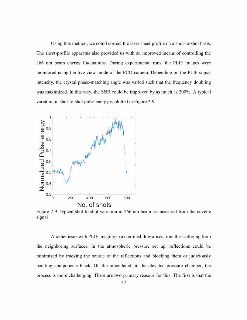
47
Using this method, we could correct the laser sheet profile on a shot-to-shot basis.
The sheet-profile apparatus also provided us with an improved means of controlling the
266 nm beam energy fluctuations. During experimental runs, the PLIF images were
monitored using the live view mode of the PCO camera. Depending on the PLIF signal
intensity, the crystal phase-matching angle was varied such that the frequency doubling
was maximized. In this way, the SNR could be improved by as much as 200%. A typical
variation in shot-to-shot pulse energy is plotted in Figure 2-9.
Figure 2-9 Typical shot-to-shot variation in 266 nm beam as measured from the cuvette
signal
Another issue with PLIF imaging in a confined flow arises from the scattering from
the neighboring surfaces. In the atmospheric pressure set up, reflections could be
minimized by tracking the source of the reflections and blocking them or judiciously
painting components black. On the other hand, in the elevated pressure chamber, the
process is more challenging. There are two primary reasons for this. The first is that the

48
laser sheet correction method could not take into account any possible change in the laser
sheet profile due to dust at the flat windows. In particular, we observed that the laser sheet
profile in the cuvette and the mixing tube were not the same. The second is that the
scattering from the windows and the inner walls of the pressure chamber could induce
additional background in the PLIF images, which could not be accounted for by the sheet
correction. In order to reduce this background interference, the pressure chamber windows
were almost entirely blocked except for a slit that allowed the laser sheet to enter the
pressure chamber. A sample background-corrected PLIF image is shown in Figure 2-8.
The colorbar indicates the pixel value. The vertical straight lines in the region 6 mm < r <
8 mm are due to the scattering that cannot be corrected even by shot-to-shot correction.
Figure 2-10 Background-corrected PLIF image for methane-air mixing at 3 atm, Reh =
18600.
49
2.3.2.3 Fuel air ratio determination
The acetone fluorescence signal F(x,y) is directly proportional to the local laser
fluence and concentration of acetone. In general, the acetone fluorescence depends on the
local temperature, but in the current study this method is primarily used under isothermal
conditions. The pixel intensity I(x,y) in a PLIF image is the sum of background, intrinsic
camera noise and the fluorescence. The background noise is usually related to scattering
from surfaces and windows, or fluorescence from unintended sources such as windows or
paints. The intrinsic noise in the camera is mainly due to readout noise [73]. To separate
the fluorescence signal, the background signal is subtracted from the PLIF image. The
background image B(x,y) is obtained by capturing the image without any acetone present
in the flow field. The background signal is shot-dependent and any shot-to-shot variation
in laser energy causes it to fluctuate. It is not an issue when the fluorescence is an order of
magnitude higher than the background, however in fuel-air mixing for very lean patches,
it can lead to significant error. Thus, accounting for shot-to-shot variation helps in reducing
the background noise. The shot-adjusted background signal has been used in this study.
Once this image is subtracted from the shot-adjusted PLIF images, the resulting signal is
an outcome of the fluorescence from the acetone. To obtain ‘pure-fuel’ fluorescence, the
mixing tube is filled with acetone-saturated air. The mixing tube is plugged with an annular
Teflon plug and “pure-fuel” is added to the mixing tube. This pure-fuel signal P(x,y) is
then corrected for the shot-to-shot variation in the laser pulse. The shot-adjusted
background signal is then subtracted from the shot-adjusted pure-fuel signal. The resulting
image provides the fluorescence from the maximum concentration of acetone. The fuel-air
ratio at a point can be calculated by dividing the shot-adjusted background-corrected PLIF
signal of fuel-air mixture with the corresponding pure-fuel pixel value. The final image
provides the spatial distribution of fuel-air ratio in the mixing tube.

50
For these experiments, the SNR is found to be in the range of 24-30 in fuel-rich
regions, while in fuel-lean regions the signal could be as low as the background. The
fluorescence data is affected by the laser sheet absorption as it passes through the field of
view. In addition, the scattering off the inner-wall of the mixing tube and hence the
background signal may vary from shot-to-shot because of fluorescence itself. These factors
are relatively low in magnitude (<10%) and difficult to correct for. Hence, the image
processing does not account for these errors.
2.3.3 PARTICLE IMAGE VELOCIMETRY
High speed stereoscopic PIV measurements were taken during the flashback runs.
A pair of Nd:YLF lasers (Coherent Evo 90) were used to get a pair of laser pulses which
were combined and expanded into a laser sheet entering the swirl combustor from the top.
This arrangement of laser sheet allowed the illumination of the boundary layer on the
center-body without much scattering off the wall. By bringing the laser sheet from the top,
the forward scattering of laser sheet was captured by high speed cameras (Photron APX).
These high-speed cameras were tilted with respect to the laser sheet. Hence, to keep the
particles in focus, scheimpflug adapters were mounted on the camera. These adapters were
adjusted to satisfy the scheimpflug criterion. This arrangement of the laser sheet and the
cameras are illustrated in the schematic as shown in Fig 2-11. A set of digital delay
generators (SRS DG535) were used to sync the lasers such that there is a delay of 80
microseconds between laser pulses. At the same time, camera trigger and the frame rates
were adjusted such that both cameras capture simultaneous particle images. These cameras
were operated in “End” trigger mode which allowed the data to be captured with a manual
trigger. Camera operations were controlled using Photron software (PFV 0.63).

51
Figure 2-11 Optical diagnostic set up for elevated pressure experiments
A digital delay generator (SRS DG535) was used to provide a delay of 80 µs between laser
pulses. The laser sheet thickness was kept at 1mm FWHM. The field of visualization
extended from z = -80mm to z = -55mm where the z-coordinate is measured relative to the
exit of the mixing tube. A calibration target of size 10 mm x 40 mm with dot spacing of 1
mm was translated normal to the measurement plane in the steps of 0.5 mm. Solid and
liquid seeding particles were used to Mie-scatter the laser on to the particle imaging
cameras. For liquid particle seeding, air flow is seeded with olive oil droplets of nominal
diameter size of 1 micron. These olive particles are generated by flowing a fraction of air
flow through the six-jet atomizer (TSI). For solid particle seeding, titanium oxide particles
with nominal diameter of 1 micron were used. For this purpose, a copper fluidized bed

52
seeder was used to generate a uniformly seeded air flow. During experimental runs with
solid seeding particles, the mixing tube inner wall would get covered with a fine layer of
particles. So, after 2-3 runs, the combustor was disassembled to clear the mixing tube walls.
For this inconvenience, the elevated pressure chamber experiments were carried out using
liquid seeding particles.
The Mie scattering from the particles was captured as images of size 256 x 512
pixels at 8 kHz. Since the Mie scattering was imaged through a curved surface, the resulting
distortion was corrected by applying a 3rd order polynomial mapping function obtained by
the calibration.
2.3.3.1. Particle Image Processing
The three-component planar velocity field was calculated on the basis of two
subsequent Mie scattering images taken at 8 kHz using the LaVision DaVis software
package. The interrogation window size was 16x16 pixels corresponding to 0.8 x 0.8 mm²
in physical space. A 75% overlap was chosen to get a larger number of vectors in the
vicinity of the flame front (based on vaporized droplets). The distance between the wall
and the first velocity vector in the radial direction was about 0.5 mm. The calibration
process included correcting the images for geometrical distortion induced by the curvature
of the mixing tube walls. For the current experiment, a fused-silica tube with high optical
homogeneity (i.e., no lengthwise striations) was used to minimize optical defects.
Entry of the PIV laser sheet from the top of the mixing tube ensured that PIV
measurements could be made near the center-body surface with a minimum of scattering.
Reducing the scattering is more important with PIV than with PLIF since the laser light
and scattered light are at the same frequency and so cannot be distinguished. This
orientation of the laser sheet worked well at atmospheric pressure, but at higher pressure,
53
striations in intensity appeared in the particle scattering images. These intensity striations
were random in nature and were caused by the sheet passing through the swirl flame and
exhaust gases. This effect increased at higher pressures owing to the larger gradients
associated with the higher Reynolds numbers. Example striations in the particle scattering
images are shown in Fig 3(a). The resulting striated particle fields are problematic for PIV
since they cause the cross-correlation peaks to have a two-dimensional character. Figure
3(a) shows a sample cross correlation map calculated at a location with striations and
exemplifies the elongated cross-correlation function. To mitigate this effect, the intensity
profile was corrected by first filtering the vertical sliding background of size 16 pixels and
then applying min-max normalization filter. The resulting image had a relatively uniform
particle image. A sample correlation maps for a sheet-corrected image is shown in Figure
3. The corrected image shows axisymmetric correlation peaks, as is expected for round
particle images. This operation greatly improves the quality of the resulting PIV data, as
shown in Fig 8(b).
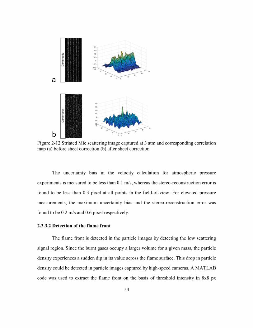
54
Figure 2-12 Striated Mie scattering image captured at 3 atm and corresponding correlation
map (a) before sheet correction (b) after sheet correction
The uncertainty bias in the velocity calculation for atmospheric pressure
experiments is measured to be less than 0.1 m/s, whereas the stereo-reconstruction error is
found to be less than 0.3 pixel at all points in the field-of-view. For elevated pressure
measurements, the maximum uncertainty bias and the stereo-reconstruction error was
found to be 0.2 m/s and 0.6 pixel respectively.
2.3.3.2 Detection of the flame front
The flame front is detected in the particle images by detecting the low scattering
signal region. Since the burnt gases occupy a larger volume for a given mass, the particle
density experiences a sudden dip in its value across the flame surface. This drop in particle
density could be detected in particle images captured by high-speed cameras. A MATLAB
code was used to extract the flame front on the basis of threshold intensity in 8x8 px

55
windows with 75% overlap. For the particle images captured at 3 atm, striations were
filtered out as described earlier. Then, a smoothing spatial filter was applied to get rid of
high-frequency signals due to the discrete nature of the particle images. Afterwards, the
image was binarized on the basis of a cut off intensity. Any morphological opening in the
binarized image was corrected by taking the binarized version of the inverted image and
then remove any gaps in the detected flame front. Then, an edge detection routine was
applied to get the flame front location. It should be noted that the filtering also averages
out the sub-millimeter flame structures which might exist in highly turbulent flames. Fig
2-13 shows the flame surface detection for hydrogen-rich flame flashback. The gamma
correction of image is carried out to reveal the particles in burnt gases. The flame edge
detection routine is successful in detecting wrinkled flame profiles.
Figure 2-13 Flame edge detection on the basis of seeding particle density
Determination of flame front at elevated pressure remained challenging,
particularly due to the presence of striations in the flow field. These striations were
dynamic in nature and would cause the local fluence of the laser to low in certain parts of

56
the particle images A sample particle image of elevated pressure flame is shown in Figure
2-14. In the regions marked with red ellipse it is difficult to mark the flame surface profile.
Figure 2-14 Striated particle image during the elevated pressure flashback of methane-air
swirl flames
Thus, the striations in the particle images affect not only the PIV as discussed in
the previous subsection, but they also affect the determination of the flame front. This issue
becomes even severe with hydrogen-rich flames at elevated pressure since the flame
wrinkling is very strong in the hydrogen-air flames.

57
CHAPTER 3 : PREMIXED FLAME FLASHBACK
This chapter is dedicated towards developing a three-dimensional understanding of
the flame-flow interaction during swirl flame flashback. The swirling flame tongue during
the flashback is unique in the sense that different regions of the flame tongue interact with
the approach flow in different ways. This aspect of flame-flow interaction is analyzed by
constructing a quasi-three-dimensional flame surface and the flow field around it. Later, in
this chapter, we discuss the interaction from the flame’s frame of reference.
3.1 Swirl flame flashback: A unique scenario
3.1.1 ASYMMETRICAL SITUATION IN AZIMUTHAL DIRECTION
Typically, flashback is conceptualized for the case where the oncoming flow opposes the
direction of propagation of the flame [6], [58], [51], [74]. However, in swirl-flame
flashback, which can be led by a three-dimensional flame tongue, the nature of the flame-
flow interaction differs for different parts of the flame tongue. Figure 3-1 shows a
schematic of a propagating flame tongue in front and top view. The motion of the flame
tongue is marked with red arrow while the motion of the upstream fluid is marked with
black arrows. The leading or the front side of the flame tongue is defined as the side which
leads the propagation. It is marked with a green rectangle in Fig 3-1. The aft end or the
trailing edge of the flame tongue is marked with a pink rectangle. On this end, the flame
surface normal and upstream flow oppose each other. On the contrary, the leading side of
the flame tongue has the flame surface normal and the upstream flow aligned in the same
direction.
Results in this chapter has been published in the following article:
Rakesh Ranjan, Dominik F Ebi, Noel T Clemens, Role of inertial forces in flame-flow interaction during premixed swirl flame
flashback, Proceedings of the Combustion Institute, 2018,ISSN 1540-7489, https://doi.org/10.1016/j.proci.2018.09.010. Dr. Ebi conducted the flashback experiments, while the post-processing of data, development of frozen-flame assumption and the
analysis of velocity fields were done by Rakesh Ranjan.
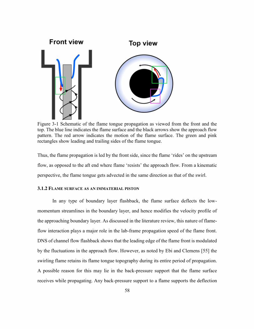
58
Figure 3-1 Schematic of the flame tongue propagation as viewed from the front and the
top. The blue line indicates the flame surface and the black arrows show the approach flow
pattern. The red arrow indicates the motion of the flame surface. The green and pink
rectangles show leading and trailing sides of the flame tongue.
Thus, the flame propagation is led by the front side, since the flame ‘rides’ on the upstream
flow, as opposed to the aft end where flame ‘resists’ the approach flow. From a kinematic
perspective, the flame tongue gets advected in the same direction as that of the swirl.
3.1.2 FLAME SURFACE AS AN IMMATERIAL PISTON
In any type of boundary layer flashback, the flame surface deflects the low-
momentum streamlines in the boundary layer, and hence modifies the velocity profile of
the approaching boundary layer. As discussed in the literature review, this nature of flame-
flow interaction plays a major role in the lab-frame propagation speed of the flame front.
DNS of channel flow flashback shows that the leading edge of the flame front is modulated
by the fluctuations in the approach flow. However, as noted by Ebi and Clemens [55] the
swirling flame retains its flame tongue topography during its entire period of propagation.
A possible reason for this may lie in the back-pressure support that the flame surface
receives while propagating. Any back-pressure support to a flame supports the deflection

59
of the approach flow thereby creating favorable conditions for flame surface to move in
the lab-frame. Thus, a continuously back-supported flame surface would have a preferred
shape towards the approach flow owing to the continuous deflection of the streamlines in
the approach flow. Experiments by Dreizler’s group have shown the existence of elevated
back-pressure during swirling flame flashback [75]. The existence of back-pressure has
also been found to be true in flames which propagate along the vortex axis [16].
The deflection of the oncoming flow streamlines by the flame means that unlike
the pure kinematic picture of flame as envisaged by the classical Lewis and von Elbe
model, the flame deflects the streamlines, and this helps in the flame propagation. This
deflection or the push from the flame surface acts not only towards opposing the approach
flow but also towards adding to the momentum of the upstream flow, especially in the case
of swirling flame flashback. For example, in the top view of Fig 3-1, the flame would push
the upstream flow in azimuthal direction because the flame tongue and the upstream flow
is moving in the same direction. This action of flame on the upstream flow is akin to
‘sweeping’ (dynamic interaction) in addition to the ‘riding’ (kinematic effect). The
sweeping type interaction would not be apparent in the front view of Figure 3-1, since the
flame normal and the flow do not point in the same direction. The discussion in the existing
research literature, so far, is based on the picture presented in the front view.
To investigate the flame-flow interaction, we make certain assumptions which
allow us to reconstruct the three-dimensional flow field from planar three-component PIV
data. This method is described in the next subsection.

60
3.2 Flame-flow interaction: the three-dimensional picture
3.2.1 FLAME SURFACE TOPOLOGY
Previous studies have shown that the upstream propagation of the flame during
swirl flame flashback is characterized by a unique three-dimensional shape of the flame
surface [76]. We call it a flame tongue due to its convex aerodynamic shape which has a
well-defined leading point i.e. the flame tip. While studying flame-flow interaction, it
becomes necessary to define different regions of the flame surface since the interaction is
location-specific. It also becomes necessary to define how the flow approaches the flame
surface. Thus, the entire neighborhood space of the flame tongue needs to be defined.
Figure 3-2 Schematic of the flame topology
Different regions on the flame surface are named on the basis of the flame
movement in lab-frame. This nomenclature is illustrated in Figure 3-2. The motion of the
flame tongue is marked with a blue arrow. The flame tongue is the entire flame surface in
turquoise color. The leading edge of the flame is the forward side of the flame surface
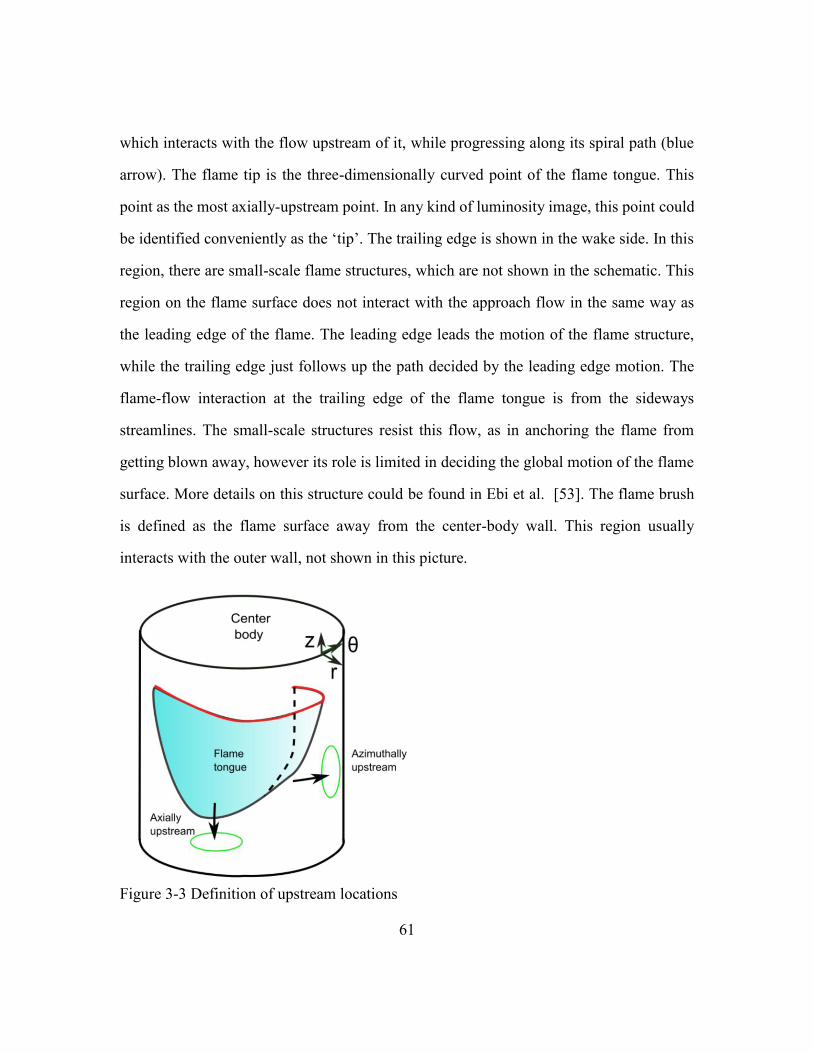
61
which interacts with the flow upstream of it, while progressing along its spiral path (blue
arrow). The flame tip is the three-dimensionally curved point of the flame tongue. This
point as the most axially-upstream point. In any kind of luminosity image, this point could
be identified conveniently as the ‘tip’. The trailing edge is shown in the wake side. In this
region, there are small-scale flame structures, which are not shown in the schematic. This
region on the flame surface does not interact with the approach flow in the same way as
the leading edge of the flame. The leading edge leads the motion of the flame structure,
while the trailing edge just follows up the path decided by the leading edge motion. The
flame-flow interaction at the trailing edge of the flame tongue is from the sideways
streamlines. The small-scale structures resist this flow, as in anchoring the flame from
getting blown away, however its role is limited in deciding the global motion of the flame
surface. More details on this structure could be found in Ebi et al. [53]. The flame brush
is defined as the flame surface away from the center-body wall. This region usually
interacts with the outer wall, not shown in this picture.
Figure 3-3 Definition of upstream locations

62
To specify the neighborhood of the flame tongue, we use terms such as axially
upstream to mark the region upstream in z-direction, and azimuthally upstream to show the
region of unburnt gases in the azimuthal direction. Otherwise, any reference to upstream
in this work refers to the direction of the flame normal. It implies that a region upstream of
the leading edge would be between the green ellipses in Fig 3-3, since the leading edge as
defined in previous figure is inclined with respect to the z and θ-axis. If the term is
“downstream of the flame surface”, it would mean normal to the flame surface and not the
flow.
When the discussion is in reference to the streamlines or pathlines, the term
downstream refers to the direction along the streamline or pathline. Thus, if the fluid is
moving on a spiral streamline and it is commented that it burns at a downstream location
it means that the fluid parcel moves along its path and gets burnt. This statement has no
reference to where on the flame surface it burns.
3.2.2 FLAME SURFACE RECONSTRUCTION
Over multiple flashback experiments, the global behavior of the upstream
propagation during flashback is identified as a flame tongue swirling around the center-
body in the annular space of the mixing tube. This propagating flame tongue tends to
maintain its shape and size as it moves around the center-body [47]; thus, we hypothesize
that the flame can be modeled as “frozen”. This assumption would not be valid if the flame
shape changed quickly over the timescales of observation.
The first benefit of the frozen-flame assumption is the ability to track the flame
structure as a whole, by tracking a single point on the flame surface. The three-dimensional
surface of the flame tongue allows us to uniquely define its flame tip in the luminosity
images. Hence, the flame tongue tip can be easily tracked in the luminosity images. The

63
determination of the position of the flame tongue in three-dimensions is carried out as
explained in Sec 2.3.1. Thus, by tracking the flame tip, the speed of the flame tongue, in
axial and azimuthal directions, can be determined. Figure 3-4 shows the axial position of
the flame tip for a stoichiometric methane-air flashback event. The axial velocity of the
flame tip (vztip) is nearly constant during the observation time of about 50 ms, during which
it propagated about 50 mm in the axial direction. Similarly, the angular position of the
flame tip is also tracked and the angular velocity of the flame tip (Ωtip) is also found to be
nearly constant [47].
Figure 3-4 Axial position of the flame tip during upstream propagation for a single
flashback event
It should be noted that for an aerodynamically-shaped flame tongue, the flame
speed may vary from point-to-point depending on the local flame stretch and the approach
flow speed, however for low-turbulence methane-air flashback, this effect should be
minimal.
A significant benefit of the frozen-flame assumption is that is opens up the
possibility of employing the principle of space-time equivalence. Space-time equivalence,
which is the cornerstone of Taylor’s hypothesis, means that we can map a time series to a

64
spatial profile by considering a frozen flow to be simply advected by the mean flow. In the
case where we are conducting planar imaging, such as with PIV data, the space-time
equivalence can be applied at each point in the plane. The utility of this implication is
illustrated in Fig 3-5.
Figure 3-5 a. Three instances of a flame tongue crossing the laser sheet b. Stacking of
planar flame profile to construct the flame surface
In Figure 3-5(a), the blue line in the figure marks the flame surface. The green
straight line shows the location of the laser sheet. The flame surface at three different
instances are marked with different dashes. The flame surface profile that crosses the laser
sheet at instants t0 – Δt, t0 and t0 + Δt could be stacked in space by shifting the flame profile
by vztip Δt and Ωtip Δt in axial and azimuthal directions, respectively. It should be noted that
in this case, the PIV repetition rate must be smaller than the time-scales over which flame
surface changes. In the current set of data, the flame profiles were extracted from particle
images of size 256 x 512 pixels. The decrease in particle density across the flame front
served as the marker for the flame surface. Particle images were captured every 250
microseconds, while the leading-edge topography was found to sustain over 20-30
milliseconds. The flame structures at the trailing edge of the flame tongue are usually of
smaller size and time scales, and hence difficult to reconstruct. For propagating flames, the
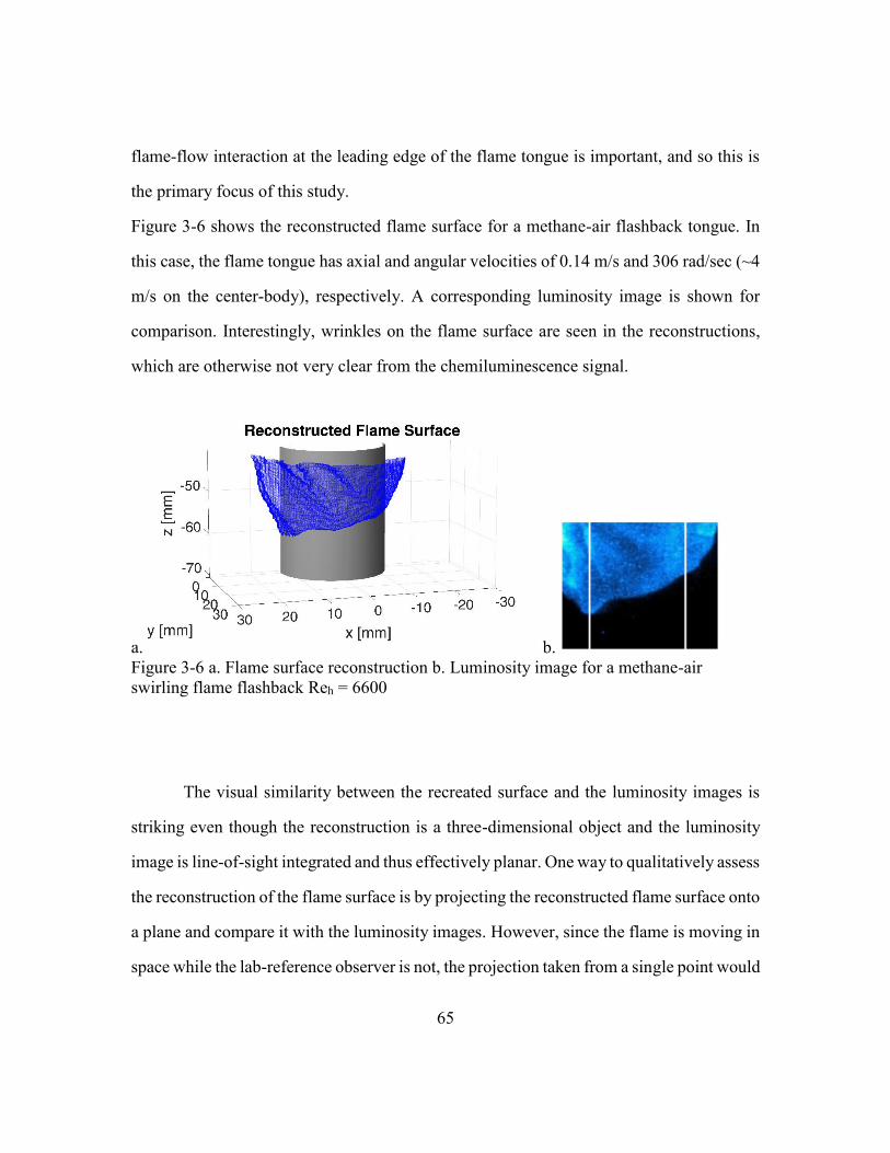
65
flame-flow interaction at the leading edge of the flame tongue is important, and so this is
the primary focus of this study.
Figure 3-6 shows the reconstructed flame surface for a methane-air flashback tongue. In
this case, the flame tongue has axial and angular velocities of 0.14 m/s and 306 rad/sec (~4
m/s on the center-body), respectively. A corresponding luminosity image is shown for
comparison. Interestingly, wrinkles on the flame surface are seen in the reconstructions,
which are otherwise not very clear from the chemiluminescence signal.
a. b.
Figure 3-6 a. Flame surface reconstruction b. Luminosity image for a methane-air
swirling flame flashback Reh = 6600
The visual similarity between the recreated surface and the luminosity images is
striking even though the reconstruction is a three-dimensional object and the luminosity
image is line-of-sight integrated and thus effectively planar. One way to qualitatively assess
the reconstruction of the flame surface is by projecting the reconstructed flame surface onto
a plane and compare it with the luminosity images. However, since the flame is moving in
space while the lab-reference observer is not, the projection taken from a single point would

66
provide only a single frame for comparison. For example, in Figure 3-6, the projected view
of the reconstructed flame surface is chosen such that it appears similar to the luminosity
image. The visual similarity would not be apparent for a different view of the reconstructed
surface.
A way to circumvent this issue is by taking the projection of the reconstructed flame
surface from different vantage points. Since we already know the lab-frame velocity of the
flame structure (vztip in axial direction, Ωtip in azimuthal direction), if the vantage point
moves with the - vztip and - Ωtip then the projections comparable to that of the instantaneous
luminosity images could be obtained.
To obtain these projections, a view transformation matrix corresponding to a
vantage point is calculated in MATLAB and applied to the three-dimensional flame
surface. This routine is repeated for vantage points that are shifted by - ΩtipΔt in the
azimuthal direction. The camera elevation is set at 5 degrees for all projections. The
resulting projection obtained gives a recreated line-integrated signal of the reconstructed
flame surface. It should be noted that this method is only approximate since the local
luminosity of a flame surface is dependent on more factors than just geometry, but the
luminosity signal is sufficient to mark the presence of the flame along a line-of-sight. Thus,
it can be used to mark the leading flame edge as seen from a given vantage point, which
enables us to compare the flame tongue leading edge in the experimentally observed
luminosity images and projections of the reconstructed surface. The fitting of the leading
edges was found to match within ±1 mm in the vicinity of the laser sheet location. Figure
3-7 shows a comparison of the luminosity images and the projections from reconstructions
at the instants when the flame swirls towards the front of the center-body.

67
Figure 3-7 Comparison of the luminosity images and the projections from reconstructed
flame surface. Each frame is taken 1 millisecond apart. The trailing edge of the flame
tongue is not reconstructed.
From Figure 3-7(a) – (c) we see the flame tongue has not even crossed the laser sheet
location (midline of the image) and yet, the flame surface projection created by the frozen
flame assumption recreates the leading edge with remarkable similarity. This observation
affirms that the flame moves as a single structure and maintains a nearly constant axial and
angular velocity.
3.2.3 FLOW FIELD RECONSTRUCTION
Premixed flames respond to the local flow environment, an example of which is the
wrinkling associated with a flame that propagates in a turbulent flow. Hence, the premixed
flame surface is inherently coupled to the flow upstream of it. Therefore, a frozen flame
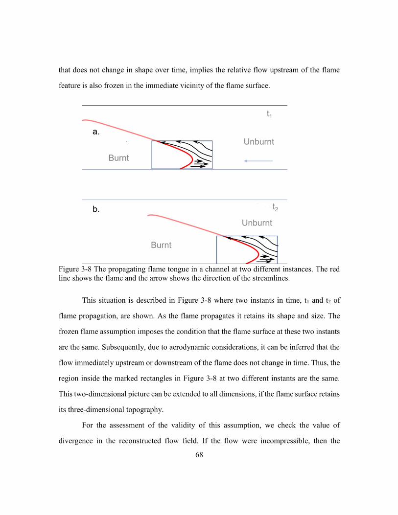
68
that does not change in shape over time, implies the relative flow upstream of the flame
feature is also frozen in the immediate vicinity of the flame surface.
Figure 3-8 The propagating flame tongue in a channel at two different instances. The red
line shows the flame and the arrow shows the direction of the streamlines.
This situation is described in Figure 3-8 where two instants in time, t1 and t2 of
flame propagation, are shown. As the flame propagates it retains its shape and size. The
frozen flame assumption imposes the condition that the flame surface at these two instants
are the same. Subsequently, due to aerodynamic considerations, it can be inferred that the
flow immediately upstream or downstream of the flame does not change in time. Thus, the
region inside the marked rectangles in Figure 3-8 at two different instants are the same.
This two-dimensional picture can be extended to all dimensions, if the flame surface retains
its three-dimensional topography.
For the assessment of the validity of this assumption, we check the value of
divergence in the reconstructed flow field. If the flow were incompressible, then the

69
divergence value should be zero everywhere; however, at the flame surface, the dilatation
should cause the divergence to be non-zero. In Figure 3-9 (a), we show the distribution of
the normalized divergence values in the reconstructed flow field in the incoming unburnt
gases only.
Figure 3-9 Divergence value distribution in the reconstructed flow field with a. only
unburnt gases b. unburnt, burnt and flame surface
The divergence is normalized by the maximum gradient in the mean velocity profile. The
resulting distribution is normal and has a standard deviation of 0.1. In Figure 3-9(b), the
divergence distribution is shown for all regions irrespective if they are unburnt or burnt.
As is clear, the distribution is not symmetric and the tail on the positive side extends farther
with the skewness value of 0.75. This observation is expected since the divergence near
the flame front is expected to be positive owing to dilatation effects.
Figure 3-10 shows the isosurface plots of the normalized divergence value of 0.4 and 0.6
in the reconstructed flow field. It is evident that large divergence values exist very close to
the flame surface. This observation gives us confidence that the reconstruction of the flow
field satisfies the physics associated with the flow.

70
Figure 3-10 Isosurface plot of normalized divergence value of a. 0.4 and b. 0.6. Pockets
of high divergence are marked with a red circle
There are scattered pockets of large-divergence in the flow field (red circled in
Figure 3-10(a)), however they lie close to the outer wall, away from the leading edge of
the flame. These large-divergence values at large radial locations are a result of stacking
the velocity data in given azimuthal steps, which at large radial locations increases the grid
spacing. At smaller radial locations, this error is smaller. Thus, under the frozen flow
assumption, the reconstructed flow field is - at best – “quasi-instantaneous” in nature. In
regions away from the flame surface, or at large radial locations, the three-dimensional
stitching of the velocity field would not be valid. In highly turbulent conditions, the flow
field reconstruction in the azimuthal direction would require highly-resolved data to enable
any kind of out-of-plane reconstruction.
The reconstructed flame surface and the quasi-instantaneous flow provides us the
complete three-dimensional flame surface and flow field during flashback, albeit under the
frozen flame-flow assumption. In subsequent subsections, we use these data to discuss the
nature of flame-flow interaction for these low-turbulence cases. We mention the pathlines
and streamlines constructed using the quasi-instantaneous flow as quasi-pathlines and
quasi-streamlines respectively.
Flame
surface
a. b.
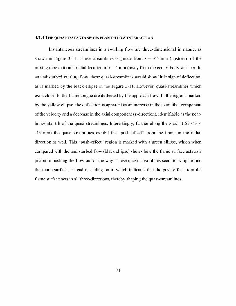
71
3.2.3 THE QUASI-INSTANTANEOUS FLAME-FLOW INTERACTION
Instantaneous streamlines in a swirling flow are three-dimensional in nature, as
shown in Figure 3-11. These streamlines originate from z = -65 mm (upstream of the
mixing tube exit) at a radial location of r = 2 mm (away from the center-body surface). In
an undisturbed swirling flow, these quasi-streamlines would show little sign of deflection,
as is marked by the black ellipse in the Figure 3-11. However, quasi-streamlines which
exist closer to the flame tongue are deflected by the approach flow. In the regions marked
by the yellow ellipse, the deflection is apparent as an increase in the azimuthal component
of the velocity and a decrease in the axial component (z-direction), identifiable as the near-
horizontal tilt of the quasi-streamlines. Interestingly, further along the z-axis (-55 < z <
-45 mm) the quasi-streamlines exhibit the “push effect” from the flame in the radial
direction as well. This “push-effect” region is marked with a green ellipse, which when
compared with the undisturbed flow (black ellipse) shows how the flame surface acts as a
piston in pushing the flow out of the way. These quasi-streamlines seem to wrap around
the flame surface, instead of ending on it, which indicates that the push effect from the
flame surface acts in all three-directions, thereby shaping the quasi-streamlines.

72
Figure 3-11 Instantaneous quasi-streamlines in front of the flame surface. These
streamlines emanate in the boundary layer along the center-body
3.2.4 QUASI-PATHLINES
A logical way to understand the flame-flow interaction is to investigate it from the
perspective of streamlines that get disturbed due to the approach flow, as discussed above.
An even better way to understand it is to track a fluid parcel starting in the oncoming flow
and see how it gets affected by the flame surface. For an unsteady flow, the instantaneous
streamlines are not the same as the pathlines [77]. For example, if in the previous
subsection (Figure 3-9), one treats the quasi-streamlines as the quasi-pathlines, the fluid
parcels approaching the flame surface would appear to escape the fate of getting burnt since
the quasi-streamlines wrap around the flame surface. This picture plainly ignores the fact
that the flame surface is also moving. If one tracks the fluid parcel’s movement in space, a
simultaneous estimation of flame surface motion would also be needed to understand how
the fluid-parcel and the flame interact. In other words, it is necessary to know how the fluid
parcel moves with respect to the flame surface.

73
Owing to these considerations, it is useful to view the flow from the frame-of-
reference of the flame. While defining the flame’s frame of reference itself can be a
challenging task, it is well-defined for a propagating swirl flame tongue. We have already
obtained the velocity of the flame tongue, and therefore to analyze the flow from the
flame’s frame of reference, we must subtract the flame’s velocity from the fluid velocity
field. In the flame’s frame of reference, the flow is steady (ignoring turbulence), and so
quasi-pathlines and quasi-streamlines are the same. Thus, the fluid particle movement can
be tracked in space.
Figure 3-12 Quasi-streamlines in flame’s frame of reference
In the flame’s frame of reference, quasi-streamlines are the same as quasi-pathlines.
Thus, in the following discussion these pathlines shall be referred to as streamlines, unless
specified otherwise. Figure 3-12 shows the quasi-streamlines in the approach flow as seen
from the flame’s frame of reference. The radial and axial points of streamline initiation is
the same as that in Figure 3-11. However, unlike the quasi-streamlines in the lab-frame
74
which move away from the flame surface, the quasi-streamlines in the flame-frame
approach the flame surface. This picture tells us that the flame moves faster than the flow
upstream of it. It is also seen that as the quasi-streamlines approach the leading edge of the
flame, they diverge (shown in red ellipse). This divergence indicates that the oncoming
flow decelerates upstream of the flame tongue, in the axial as well as the azimuthal
direction. On the other hand, in the lab-frame, the flame is found to cause an acceleration
of the approach flow in the azimuthal direction while it slows down the flow in the axial
direction, as illustrated in Figure 3-11. As discussed at the start of this chapter, the lab
frame can be misleading when considering the flame-flow interaction. Evidence for this is
that in the flame’s frame of reference the flame causes deceleration of the approach flow
in both the axial and azimuthal directions.
3.2.5 NON-INERTIAL FRAME OF REFERENCE
In the previous subsection, we noted that the quasi-streamlines diverge as they
approach the flame tongue’s leading edge. To further analyze this kind of interaction, we
investigate the motion of any fluid parcel approaching the flame tongue. We apply the
fundamentals of Newtonian mechanics to understand the dynamics of the interaction.
According to Newtonian mechanics, if the observer’s frame of reference is
accelerating, to satisfy the force-acceleration relation, there should be fictitious forces
applied to the mass whose motion is described in the observer’s frame. For rectilinear
motions, these forces appear only when the speed of the frame is changing in time, such as
the apparent force experienced during sudden braking of vehicles. For rotating frames of
reference, even if the angular velocity is constant, the velocity vector changes its direction
and thus the frames are accelerating in nature. In such a case, there would be a fictitious
force acting on the mass.

75
A swirling flame feature rotates in the lab-frame, and so any frame associated with
a swirling flame feature is accelerating in nature, which introduces fictitious forces such as
centrifugal and Coriolis forces. The centrifugal force acts radially outward, whereas the
Coriolis force acts perpendicular to the frame-relative velocity of the particle. These forces
are dependent on the frames of choice such that the Newtonian laws of motion are satisfied.
Centrifugal forces are often used in swirling flows to define the radial pressure gradient.
However, the Coriolis force is usually not discussed in the context of swirling flows. In the
next paragraph, we discuss its importance and its role in the flame-flow interaction.
Forces acting on a moving particle can be frame-independent, such as pressure and
viscous forces, or frame-dependent, such as centrifugal and Coriolis forces. Our choice of
frame is usually to simplify the dynamic force balance. For example, if we consider a point
mass (m) tied with a string used to rotate it around its axis with angular velocity (Ω0), we
choose to work with either from the lab-frame (inertial) or mass-frame (non-inertial). In
the lab-frame, we have centripetal acceleration (Ω02r) which acts radially inward; thus,
tension in the string is T = mΩ02r. In point mass frame of reference, the particle does not
move, but the observer’s frame is accelerating. The centrifugal force which acts radially
outward is equal to the tension T, which results in T = mΩ02r. The Coriolis force would be
zero by definition, since the relative velocity of the particle is zero. Tension in the string is
frame-independent in nature, which means that in any observer’s frame, whether moving
or not, T should be measured to be mΩ02r. The above two frames are frames of choice since
they result in direct measurement of the tension in the string.
This problem can be analyzed from a frame of reference other than the that of the
lab or the point mass. For example, let us say that the observer moves with an angular
velocity Ωf, which is different from than that of the point mass. In such a case, the
centrifugal force would be mΩf2r. In this frame, the particle is not static since it moves with
76
a relative velocity of (Ωf – Ω0)r in the direction opposite of the frame. It means that the
Coriolis force is 2mΩf(Ωf- Ω0), which acts in radially inward. Since, in this frame, the
particle velocity is also changing continuously, there would be a centripetal acceleration
given by (Ωf- Ω0)2r, which acts radially inward. Again, using the force balance equation,
the tension in the string is T = mΩf2r - 2mΩf(Ωf- Ω0) + m(Ωf- Ω0)
2r = mΩ02r, and is the same
as in the other frames. This analysis illustrates the fact that the force balance on a point
mass could be worked out in any frame of reference. However, our choice of frame (in this
case, lab-frame and mass-frame) is made in order to simplify the calculations. In the most
general case, the centrifugal force, Coriolis force and centripetal acceleration, all three
factors associated with curvilinear motion play a role in determining the dynamics of the
point mass. It should also be noted that all the forces in this example point along the radial
direction; hence, identifying these terms would simply not be possible until one correctly
knows the three-dimensional velocity field and the angular velocity of the observer’s
frame. Typically, these two factors are not known, but fortunately they are in the current
space-time reconstructions; hence, we are able to determine the fundamentals of the
dynamic balance on the point mass, which we shall later use to analyze the motion of a
fluid parcel approaching the flame tongue.
3.2.6 Regions with the maximum blockage from the flame surface
Understanding the interaction between a three-dimensionally curved flame tongue
and the swirling flow requires the assessment of the characteristic streamlines which
represent the interaction in a true manner. One needs to identify these streamlines such that
the strength of interaction could be evaluated.
Figure 3-13 illustrates the flame-flow interaction behavior at the tip and the leading
side of the flame tongue during swirl flame flashback. The red arrow indicates the direction
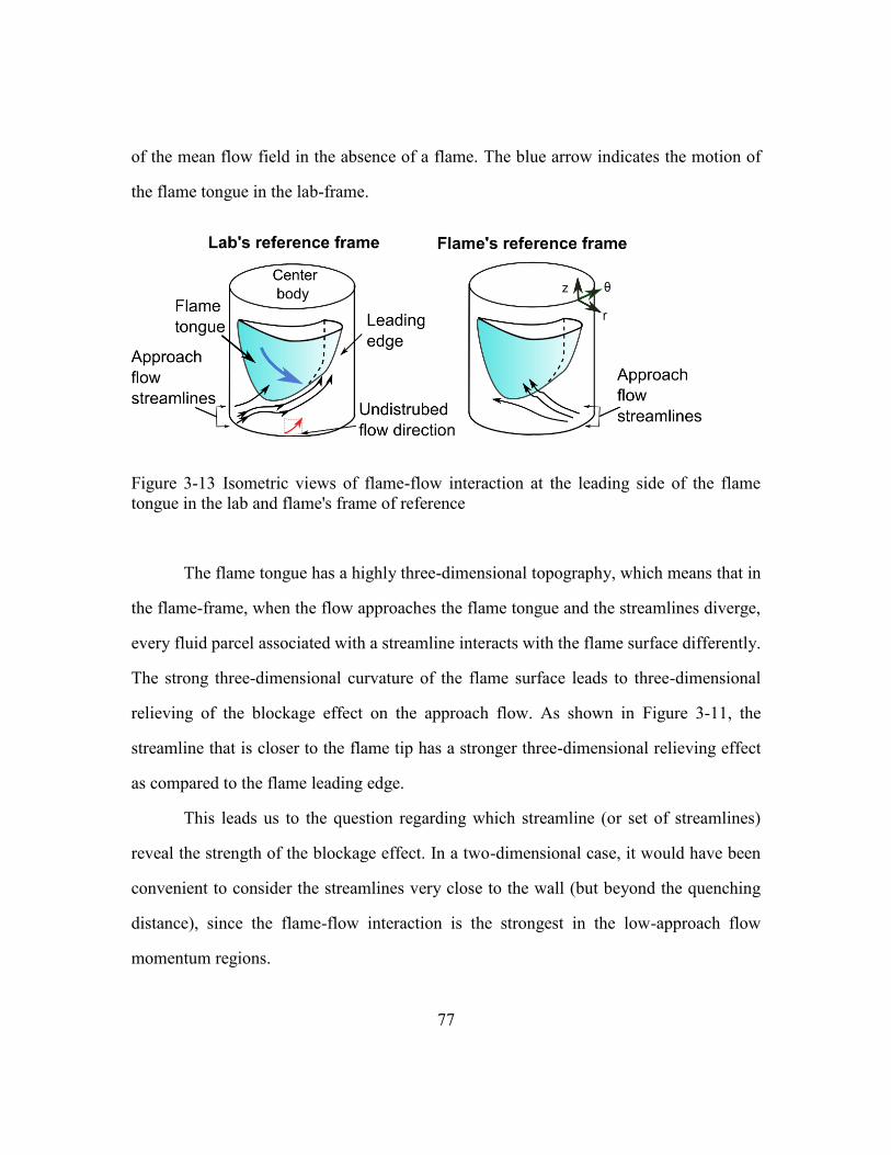
77
of the mean flow field in the absence of a flame. The blue arrow indicates the motion of
the flame tongue in the lab-frame.
Figure 3-13 Isometric views of flame-flow interaction at the leading side of the flame
tongue in the lab and flame's frame of reference
The flame tongue has a highly three-dimensional topography, which means that in
the flame-frame, when the flow approaches the flame tongue and the streamlines diverge,
every fluid parcel associated with a streamline interacts with the flame surface differently.
The strong three-dimensional curvature of the flame surface leads to three-dimensional
relieving of the blockage effect on the approach flow. As shown in Figure 3-11, the
streamline that is closer to the flame tip has a stronger three-dimensional relieving effect
as compared to the flame leading edge.
This leads us to the question regarding which streamline (or set of streamlines)
reveal the strength of the blockage effect. In a two-dimensional case, it would have been
convenient to consider the streamlines very close to the wall (but beyond the quenching
distance), since the flame-flow interaction is the strongest in the low-approach flow
momentum regions.
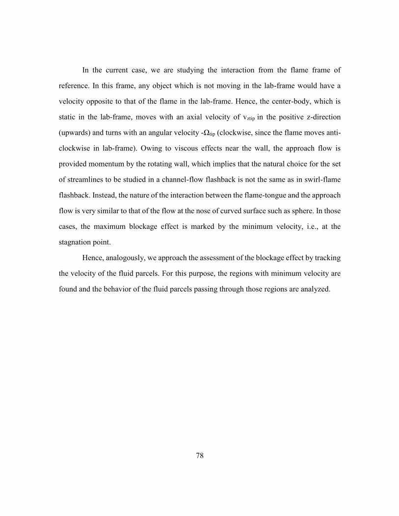
78
In the current case, we are studying the interaction from the flame frame of
reference. In this frame, any object which is not moving in the lab-frame would have a
velocity opposite to that of the flame in the lab-frame. Hence, the center-body, which is
static in the lab-frame, moves with an axial velocity of vztip in the positive z-direction
(upwards) and turns with an angular velocity -Ωtip (clockwise, since the flame moves anti-
clockwise in lab-frame). Owing to viscous effects near the wall, the approach flow is
provided momentum by the rotating wall, which implies that the natural choice for the set
of streamlines to be studied in a channel-flow flashback is not the same as in swirl-flame
flashback. Instead, the nature of the interaction between the flame-tongue and the approach
flow is very similar to that of the flow at the nose of curved surface such as sphere. In those
cases, the maximum blockage effect is marked by the minimum velocity, i.e., at the
stagnation point.
Hence, analogously, we approach the assessment of the blockage effect by tracking
the velocity of the fluid parcels. For this purpose, the regions with minimum velocity are
found and the behavior of the fluid parcels passing through those regions are analyzed.
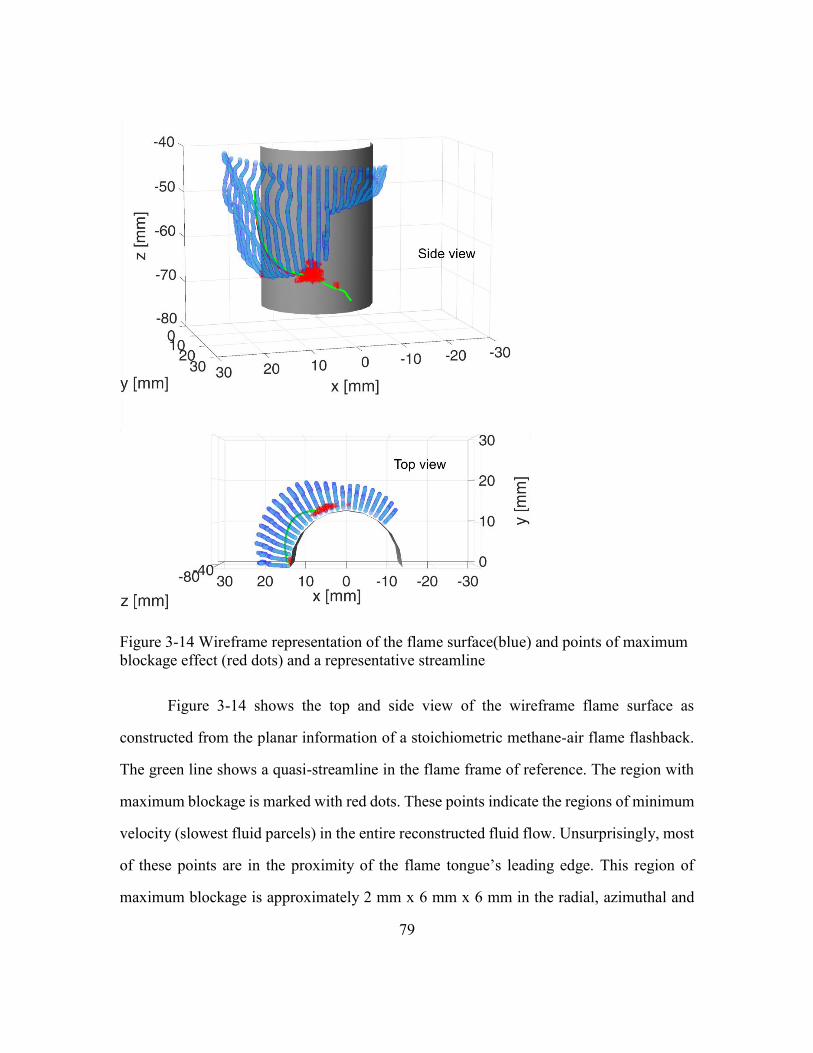
79
Figure 3-14 Wireframe representation of the flame surface(blue) and points of maximum
blockage effect (red dots) and a representative streamline
Figure 3-14 shows the top and side view of the wireframe flame surface as
constructed from the planar information of a stoichiometric methane-air flame flashback.
The green line shows a quasi-streamline in the flame frame of reference. The region with
maximum blockage is marked with red dots. These points indicate the regions of minimum
velocity (slowest fluid parcels) in the entire reconstructed fluid flow. Unsurprisingly, most
of these points are in the proximity of the flame tongue’s leading edge. This region of
maximum blockage is approximately 2 mm x 6 mm x 6 mm in the radial, azimuthal and

80
axial directions, respectively. A typical path of a fluid parcel after passing through this
volume is marked by the radially outward deflection that would not occur if not for the
blockage effect. Any such deflection also assists in the propagation of the flame since it
reduces the flame-normal approach flow velocity. In a subsequent subsection, we shall
study the kinematics of the fluid parcel that passes through the maximum blockage volume.
3.2.7 KINEMATICS OF THE FLUID PARCEL
In section 3.2.5, we discussed the role of fictitious forces arising in an accelerating
frame. While analyzing the kinematics of a fluid parcel which approaches the flame tongue,
it becomes necessary to evaluate these fictitious forces. These forces can play an important
role in determining the fluid particle path, which could be missed by an observer in the lab
frame.
Figure 3-15 shows a schematic of a quasi-pathline approaching the leading edge
of the flame tongue.
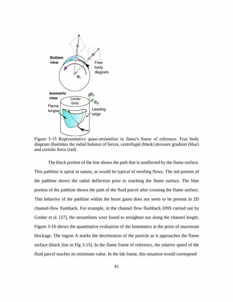
81
Figure 3-15 Representative quasi-streamline in flame's frame of reference. Free body
diagram illustrates the radial balance of forces, centrifugal (black) pressure gradient (blue)
and coriolis force (red)
The black portion of the line shows the path that is unaffected by the flame surface.
This pathline is spiral in nature, as would be typical of swirling flows. The red portion of
the pathline shows the radial deflection prior to reaching the flame surface. The blue
portion of the pathline shows the path of the fluid parcel after crossing the flame surface.
This behavior of the pathline within the burnt gases does not seem to be present in 2D
channel-flow flashback. For example, in the channel flow flashback DNS carried out by
Gruber et al. [57], the streamlines were found to straighten out along the channel length.
Figure 3-16 shows the quantitative evaluation of the kinematics at the point of maximum
blockage. The region A marks the deceleration of the particle as it approaches the flame
surface (black line in Fig 3-15). In the flame frame of reference, the relative speed of the
fluid parcel reaches its minimum value. In the lab frame, this situation would correspond
82
to the fluid parcel being pushed by the flame to nearly the same speed as that of the flame
tongue. It should be noted that towards the end of the deceleration stage, the fluid parcel is
deflected radially outward, as shown by the increase in the radial component. In stage B,
or the acceleration stage, the fluid parcel crosses the flame. The flame crossing is shown
as the red vertical line, which corresponds to the maximum divergence along the quasi-
pathline. In stage C, corresponding to the burnt gases section, the velocity components
increase, although the radial component moves to negative values, which signifies the
bending of fluid parcel paths. It should be noted that since the flame has a lab-frame
velocity in the azimuthal and axial directions only, the radial component of velocity is
unchanged for an observer in both the lab and flame frames of reference. An explanation
of this behavior of a fluid parcel would require an analysis from a Lagrangian perspective.
In next subsection, we discuss the forces acting on the fluid parcel.
Figure 3-16 Velocity components along the quasi-pathline. Red line indicates the
location of maximum divergence.
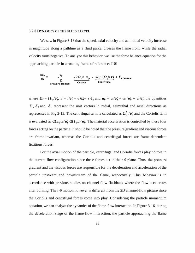
83
3.2.8 DYNAMICS OF THE FLUID PARCEL
We saw in Figure 3-16 that the speed, axial velocity and azimuthal velocity increase
in magnitude along a pathline as a fluid parcel crosses the flame front, while the radial
velocity turns negative. To analyze this behavior, we use the force balance equation for the
approaching particle in a rotating frame of reference: [10]
Dup
Dt= -
∇p
ρ⏟Pressure gradient
- 2Ωf × up⏟
Coriolis
- Ωf× (Ω
f× r)⏟
Centrifugal
+ 𝑭𝒗𝒊𝒔𝒄𝒐𝒖𝒔,
where Ωf = Ωtip 𝐞�̂�, r = r 𝐞�̂� + θ 𝐞�̂�+ z 𝐞�̂� and up = uz 𝐞�̂� + uθ 𝐞�̂� + ur 𝐞�̂�, the quantities
𝐞�̂�, 𝐞�̂� and 𝐞�̂� represent the unit vectors in radial, azimuthal and axial directions as
represented in Fig 3-13. The centrifugal term is calculated as Ωtip
2r 𝐞�̂� and the Coriolis term
is evaluated as -2Ωtipuθ 𝐞�̂� -2Ωtipur 𝐞�̂� .The material acceleration is controlled by these four
forces acting on the particle. It should be noted that the pressure gradient and viscous forces
are frame-invariant, whereas the Coriolis and centrifugal forces are frame-dependent
fictitious forces.
For the axial motion of the particle, centrifugal and Coriolis forces play no role in
the current flow configuration since these forces act in the r-θ plane. Thus, the pressure
gradient and the viscous forces are responsible for the deceleration and acceleration of the
particle upstream and downstream of the flame, respectively. This behavior is in
accordance with previous studies on channel-flow flashback where the flow accelerates
after burning. The r-θ motion however is different from the 2D channel-flow picture since
the Coriolis and centrifugal forces come into play. Considering the particle momentum
equation, we can analyze the dynamics of the flame-flow interaction. In Figure 3-16, during
the deceleration stage of the flame-flow interaction, the particle approaching the flame
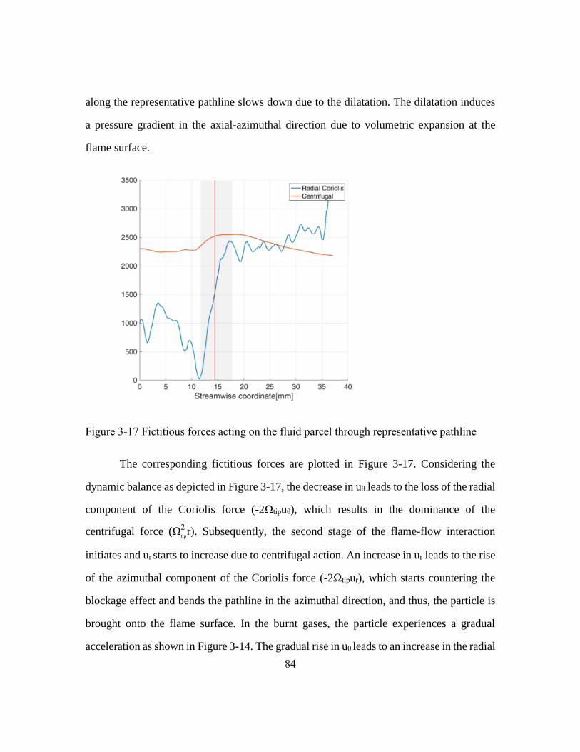
84
along the representative pathline slows down due to the dilatation. The dilatation induces
a pressure gradient in the axial-azimuthal direction due to volumetric expansion at the
flame surface.
Figure 3-17 Fictitious forces acting on the fluid parcel through representative pathline
The corresponding fictitious forces are plotted in Figure 3-17. Considering the
dynamic balance as depicted in Figure 3-17, the decrease in uθ leads to the loss of the radial
component of the Coriolis force (-2Ωtipuθ), which results in the dominance of the
centrifugal force (Ωtip
2r). Subsequently, the second stage of the flame-flow interaction
initiates and ur starts to increase due to centrifugal action. An increase in ur leads to the rise
of the azimuthal component of the Coriolis force (-2Ωtipur), which starts countering the
blockage effect and bends the pathline in the azimuthal direction, and thus, the particle is
brought onto the flame surface. In the burnt gases, the particle experiences a gradual
acceleration as shown in Figure 3-14. The gradual rise in uθ leads to an increase in the radial

85
Coriolis force. The competing centrifugal force experiences no change upon burning since
it depends on the radial location and the angular velocity of the frame. Thus, the larger
magnitude Coriolis force assists in bending of particle paths towards the center-body. The
particle moves to smaller radial location, which further reduces the centrifugal action. At
this stage, the particle continues moving in the negative radial direction. It should be noted
that the pressure gradient and viscous forces also play a role here. However, an estimation
of these terms from the available measurements would have large uncertainty.
Qualitatively, the behavior of the quasi-pathlines (Figure 3-14) is found to be
consistent across multiple experimental runs; however, the flame shape varies across these
runs. Any attempt to get the mean flame shape and the average upstream velocity field
leads to the loss of information due to the instantaneous variations in the flame-flow
interaction.
3.2.9 DYNAMIC TERMS FOR MULTIPLE QUASI-PATHLINES
Our discussion of fluid parcel kinematics and dynamics has been based on the
representative streamline. However, the dilatation-induced blockage effect of the flame is
imposed on the volume near the tip of the flame tongue, as discussed in section 3.2.6. In
this subsection, we show the Coriolis and centrifugal forces for 100 quasi-pathlines going
through the volume experiencing the flame blockage. Figure 3-18 shows the variation in
the centrifugal acceleration experienced for each of these pathlines. It is clear that most
pathlines exhibit similar behavior. Since the centrifugal acceleration is proportional to the
radial coordinate value (given the constant angular velocity of the reference frame), the
radial motion of the fluid parcel could also be inferred from this picture. It should be noted
that relative change in centrifugal force is not large (~10%). It also shows that the radial

86
deflection in the particle paths is small compared to the radial location of the particle
(approximately equal to radius of the center-body).
Figure 3-18 Variation of centrifugal term acting on the 100 different fluid particles after
the point of maximum blockage.
Figure 3-19 shows the variation in the radial component of the Coriolis force as it
crosses the point of maximum blockage. In comparison to the centrifugal force, the relative
change in the Coriolis acceleration is very large (~500%). This increase in the Coriolis term
directly corresponds to the increase in azimuthal velocity, since the reference frame has a
constant angular velocity. Interestingly, the Coriolis term has no dependence on the radial
location of the fluid parcel. It does, however, have a strong dependence on the dilatation
since it is the dilatation that induces the large relative change in velocity.
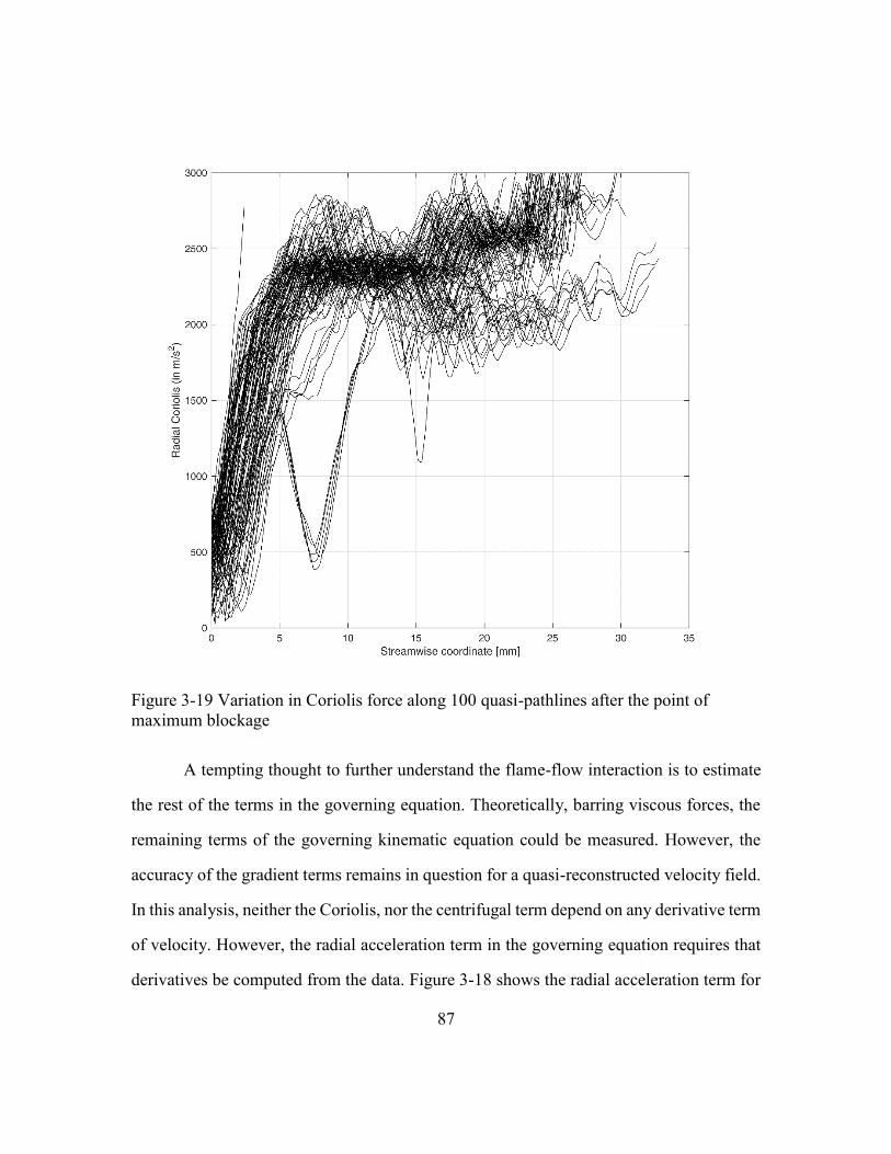
87
Figure 3-19 Variation in Coriolis force along 100 quasi-pathlines after the point of
maximum blockage
A tempting thought to further understand the flame-flow interaction is to estimate
the rest of the terms in the governing equation. Theoretically, barring viscous forces, the
remaining terms of the governing kinematic equation could be measured. However, the
accuracy of the gradient terms remains in question for a quasi-reconstructed velocity field.
In this analysis, neither the Coriolis, nor the centrifugal term depend on any derivative term
of velocity. However, the radial acceleration term in the governing equation requires that
derivatives be computed from the data. Figure 3-18 shows the radial acceleration term for
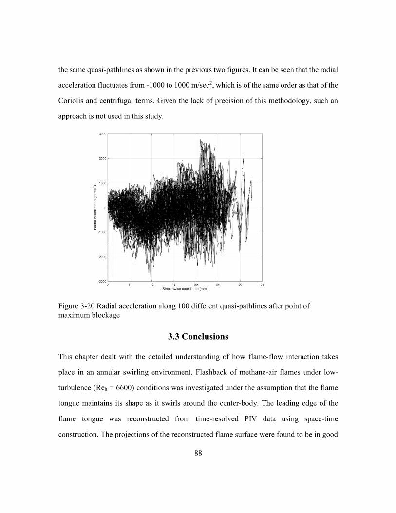
88
the same quasi-pathlines as shown in the previous two figures. It can be seen that the radial
acceleration fluctuates from -1000 to 1000 m/sec2, which is of the same order as that of the
Coriolis and centrifugal terms. Given the lack of precision of this methodology, such an
approach is not used in this study.
Figure 3-20 Radial acceleration along 100 different quasi-pathlines after point of
maximum blockage
3.3 Conclusions
This chapter dealt with the detailed understanding of how flame-flow interaction takes
place in an annular swirling environment. Flashback of methane-air flames under low-
turbulence (Reh = 6600) conditions was investigated under the assumption that the flame
tongue maintains its shape as it swirls around the center-body. The leading edge of the
flame tongue was reconstructed from time-resolved PIV data using space-time
construction. The projections of the reconstructed flame surface were found to be in good

89
match with the corresponding luminosity images. The flow field reconstruction was
assessed by computing the divergence upstream and downstream of the flame. It was noted
that the pockets of large divergence values occurred near the flame surface or at large radial
locations. Thus, it was concluded that the regions of interest in this study, i.e. the regions
close to the flame tongue leading edge were constructed well enough to construct the fluid
streamlines in the reconstructed flow field. Further, the three-dimensional quasi-
streamlines were constructed to demonstrate the blockage effect from the flame surface. It
was noted for the first time that it acts not only in radial but all three directions.
Further analysis of the flame-flow interaction was carried out from the flame frame of
reference. A fluid parcel was tracked by using the quasi-reconstructed flow field. It was
noted that the balance between the Coriolis and centrifugal terms is disturbed during the
flame-flow interaction. The change in these two fictitious forces were concomitant with
the radial bending of the representative quasi-pathline. The radial bending of the pathlines
may have some role in the generation of backpressure at the flame surface, however the
limitation in finding the gradient terms correctly did not allow us to estimate the pressure
gradient.
This understanding of the physics underlying the fluid and flame interaction also helps
us to assess how a “rich fuel-air pocket” would interact with a flame surface. This idea is
extended to the next chapter to understand how stratified flows interact with the flame
surface.
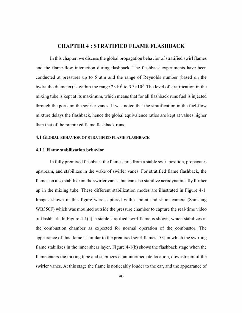
90
CHAPTER 4 : STRATIFIED FLAME FLASHBACK
In this chapter, we discuss the global propagation behavior of stratified swirl flames
and the flame-flow interaction during flashback. The flashback experiments have been
conducted at pressures up to 5 atm and the range of Reynolds number (based on the
hydraulic diameter) is within the range 2×10³ to 3.3×10⁵. The level of stratification in the
mixing tube is kept at its maximum, which means that for all flashback runs fuel is injected
through the ports on the swirler vanes. It was noted that the stratification in the fuel-flow
mixture delays the flashback, hence the global equivalence ratios are kept at values higher
than that of the premixed flame flashback runs.
4.1 GLOBAL BEHAVIOR OF STRATIFIED FLAME FLASHBACK
4.1.1 Flame stabilization behavior
In fully premixed flashback the flame starts from a stable swirl position, propagates
upstream, and stabilizes in the wake of swirler vanes. For stratified flame flashback, the
flame can also stabilize on the swirler vanes, but can also stabilize aerodynamically further
up in the mixing tube. These different stabilization modes are illustrated in Figure 4-1.
Images shown in this figure were captured with a point and shoot camera (Samsung
WB350F) which was mounted outside the pressure chamber to capture the real-time video
of flashback. In Figure 4-1(a), a stable stratified swirl flame is shown, which stabilizes in
the combustion chamber as expected for normal operation of the combustor. The
appearance of this flame is similar to the premixed swirl flames [53] in which the swirling
flame stabilizes in the inner shear layer. Figure 4-1(b) shows the flashback stage when the
flame enters the mixing tube and stabilizes at an intermediate location, downstream of the
swirler vanes. At this stage the flame is noticeably louder to the ear, and the appearance of
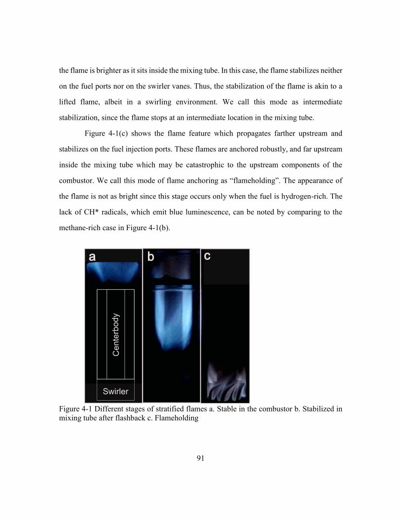
91
the flame is brighter as it sits inside the mixing tube. In this case, the flame stabilizes neither
on the fuel ports nor on the swirler vanes. Thus, the stabilization of the flame is akin to a
lifted flame, albeit in a swirling environment. We call this mode as intermediate
stabilization, since the flame stops at an intermediate location in the mixing tube.
Figure 4-1(c) shows the flame feature which propagates farther upstream and
stabilizes on the fuel injection ports. These flames are anchored robustly, and far upstream
inside the mixing tube which may be catastrophic to the upstream components of the
combustor. We call this mode of flame anchoring as “flameholding”. The appearance of
the flame is not as bright since this stage occurs only when the fuel is hydrogen-rich. The
lack of CH* radicals, which emit blue luminescence, can be noted by comparing to the
methane-rich case in Figure 4-1(b).
Figure 4-1 Different stages of stratified flames a. Stable in the combustor b. Stabilized in
mixing tube after flashback c. Flameholding

92
4.1.2 Experimental regimes
The stratified flame flashback experiments have been conducted for cases where
the mean axial velocity through the mixing tube is in the range 1.1 to 4.5 m/s. Some of the
experiments were conducted in a high-pressure facility, in which case the pressure was
varied from 1 to 5 atm. The variation in pressure allowed us to vary the Reynolds number
from 2×10³ to 3.3×10⁵, while maintaining similar volumetric flow rates and hence strain
rates and residence times. These experiments were conducted primarily to identify the
flashback regime which was described in the previous subsection.
Figure 4-2 shows the regime diagram of final stabilization modes after flashback
has occurred. The dotted curve in the plot is an approximate separation line between these
two flame stabilization modes in the mixing tube. For fuel-air mixtures with >90%
hydrogen content (by mol) always propagate all the way to the fuel ports on the swirler
vane and the flameholding takes place. At lower Reynolds numbers, the level of enrichment
required for a given equivalence ratio is lower. Similar behavior has been reported by
researchers at TU Munich, who investigated hydrogen-rich flashback in a different
geometrical configuration. [71] In their case, the fuel injection was carried out on the outer
wall and the flame stabilized itself on the fuel ports.
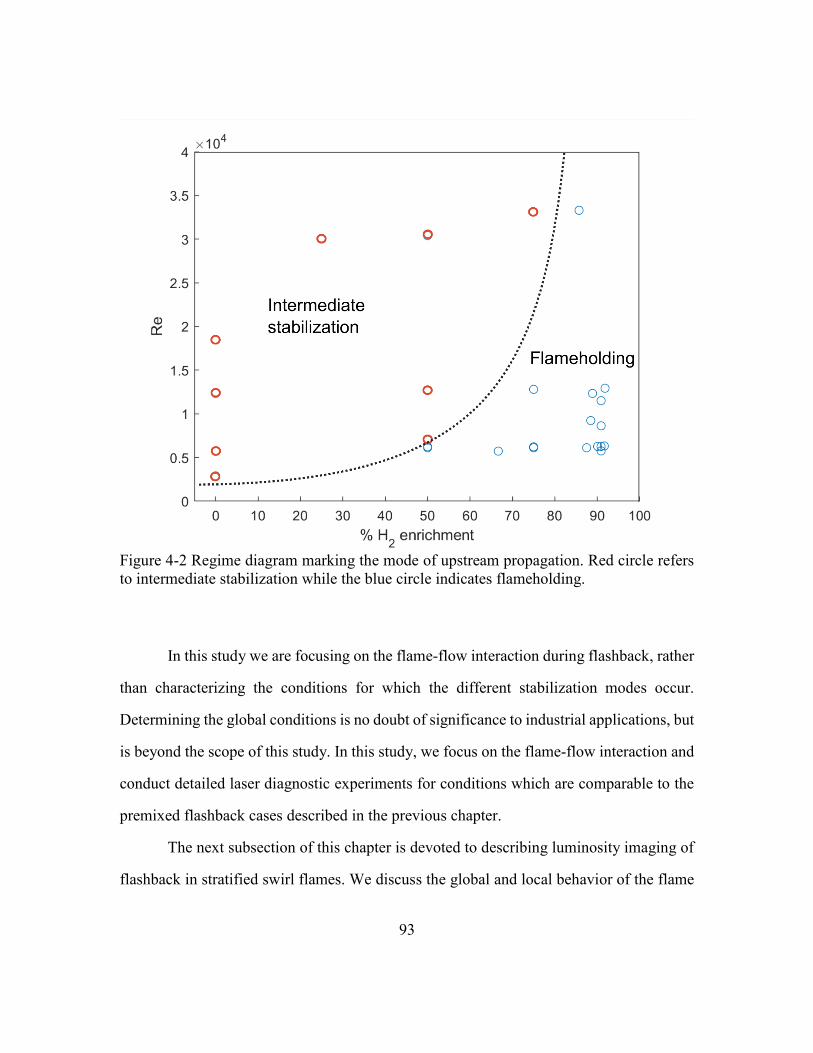
93
Figure 4-2 Regime diagram marking the mode of upstream propagation. Red circle refers
to intermediate stabilization while the blue circle indicates flameholding.
In this study we are focusing on the flame-flow interaction during flashback, rather
than characterizing the conditions for which the different stabilization modes occur.
Determining the global conditions is no doubt of significance to industrial applications, but
is beyond the scope of this study. In this study, we focus on the flame-flow interaction and
conduct detailed laser diagnostic experiments for conditions which are comparable to the
premixed flashback cases described in the previous chapter.
The next subsection of this chapter is devoted to describing luminosity imaging of
flashback in stratified swirl flames. We discuss the global and local behavior of the flame

94
surface and why it is difficult to reconstruct a three-dimensional picture of the flame
tongue, as we could do in fully premixed conditions.
4.1.3 Time-resolved luminosity imaging of the propagating flame
4.1.3.1 Intermediate stabilization
High-speed luminosity imaging of stratified flame flashback shows that flashback
is initiated in a way that is very similar to that of the premixed case. The reason for this is
that the fuel and air become progressively better mixed as they travel down the mixing
tube, until they reach a nearly premixed state at the entrance to the combustor. The typical
process for the initiation of flashback is that a large flame tongue swirls around the center-
body, sometimes dipping down and then returning, but at some point, it continues to
propagate downward along the center-body. However, after this point, the behavior of the
flame for fully premixed and stratified cases is very different. For example, for the stratified
case, as the flame moves upstream, at some point it reaches relatively unmixed fluid and
the flame surface starts to wrinkle as has been shown in previous partially-premixed flame
studies [41]. Two instances of the flame tongue swirling around the center-body are shown
in Figure 4-3. These luminosity images correspond to methane-air stratified flame
flashback at Reh = 6600. In Figure 4-3 (a), the flame tongue is an easily identifiable
structure (marked as white dashed line). The flame surface is more wrinkled but the leading
edge of the flame tongue can be identified and tracked. After 5 milliseconds, the flame
tongue moves to the central section of the view. In premixed cases, the flame tongue retains
its topology while moving in space. Furthermore, the line-of-sight integrated luminosity
signal at the leading edge shows a step increase across the flame surface, which makes it
possible identify the flame tip. This, however, is not the case with the flame tongue in the
stratified mixture. The flame surface is more non-uniform in brightness exhibiting very
95
bright pockets, while the leading edge might be very faint, as is the case shown in Figure
4-3(b). In such a case, not only does the flame tip not retain its shape but it is difficult to
identify the flame surface.
This situation leads us to the conclusion that not only is a stratified flame tongue
different in its flame-flow interaction physics, but some basic features of the flame
topology remain difficult to define. The upstream propagation of the flame stops at an
intermediate location in the mixing tube, as can be noticed in Figure 4-3. Although the
mean upstream propagation of the flame is arrested, the flame tongue still swirls around
the center-body and the global features of the flame brush seem to be moving around the
center-body. The flame surface fills the entire width of the mixing tube; however, this
situation in not axisymmetric at any instant. The flame tongue still revolves around the
center-body, even though its leading edge or the flame tip is not distinct. We did notice a
distinct sound emanating from the mixing tube during flashback that may be of interest for
future studies.
Figure 4-3 Two luminosity images captured 5 ms apart during the stratified flame flashback
of methane-air mixture. Reh = 6600.

96
4.1.3.2 Flameholding
Hydrogen-rich fuel shows a higher propensity for flameholding on the fuel-ports.
In the current set up, stratification is achieved by injecting the fuel through ports that are
close to the outer wall, as described in section 2.1 of this thesis. Prior to the occurrence of
flashback, the swirl flame is stabilized in the inner shear layer of the recirculation zone in
the combustor. The upstream propagation of the flame starts like the case of premixed
flashback. A large flame tongue propagates down the center-body as it swirls around it in
the same direction as the swirl flow. It has been reported that the hydrogen-rich flames
have smaller radial spread than the methane-air flames for fully premixed case [47]. This,
however, is not the case with stratified flames since the flame brush fills the entire radial
extent of the mixing tube. Thus, the flame brush interacts with richer fuel-air pockets in
the proximity of the outer wall. The flame propagation along the center-body occurs up to
an intermediate location in the mixing tube. So far, the global propagation behavior is
similar to that of the intermediate stabilization mode. However, the interaction of the flame
brush with the outer-wall fuel-air pockets continues. The flame brush tries to propagate
into the flammable mixtures along the outer wall and seems to succeed when the flame
encounters streaks of near-stoichiometric fuel-air pockets. Once it reaches the outer wall
the flame starts propagating along the outer wall led by acute-tipped bright flame
structures.
Figure 4-4 shows a sequence of luminosity images that are captured 5 milliseconds
apart. The formation of a flame structure along the outer wall is marked with a yellow
ellipse. In Figure 4-4(a), a locally bright flame structure that moves in the approach flow
direction (red arrow) spreads out quickly and leaves behind acute flame structures, which
anchor themselves in the outer wall boundary layer. These flame structures are pointed in
the negative streamwise direction, and are similar to the small scale structures that form in
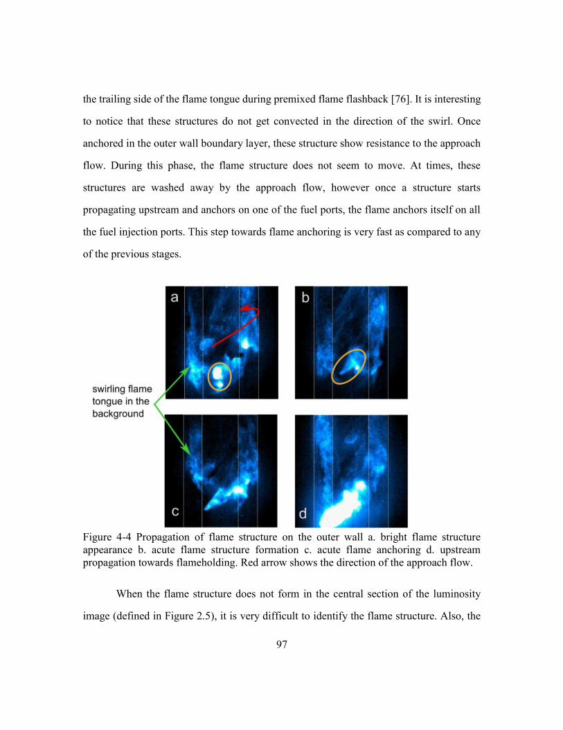
97
the trailing side of the flame tongue during premixed flame flashback [76]. It is interesting
to notice that these structures do not get convected in the direction of the swirl. Once
anchored in the outer wall boundary layer, these structure show resistance to the approach
flow. During this phase, the flame structure does not seem to move. At times, these
structures are washed away by the approach flow, however once a structure starts
propagating upstream and anchors on one of the fuel ports, the flame anchors itself on all
the fuel injection ports. This step towards flame anchoring is very fast as compared to any
of the previous stages.
Figure 4-4 Propagation of flame structure on the outer wall a. bright flame structure
appearance b. acute flame structure formation c. acute flame anchoring d. upstream
propagation towards flameholding. Red arrow shows the direction of the approach flow.
When the flame structure does not form in the central section of the luminosity
image (defined in Figure 2.5), it is very difficult to identify the flame structure. Also, the

98
formation of these acute structures is random. It requires multiple flashback runs until one
gets to capture the propagating flame structure in the central section (center-body in the
background).
Another interesting feature of stratified propagation is the simultaneous presence
of the swirling flame tongue on the center-body. It is usually difficult to decipher because
of its lower level of luminescence, but dim flame tongues on the center-body can be noted
in Figure 4-4. The flame tongues are circled with an orange ellipse in Figure 4-4. The
swirling flame tongue is on the left side of the luminosity images, although it is easier to
see in the videos than these still images. It should be noted that the initial formation of the
bright flame structure in Figure 4-4(a) occurs on the flame brush of the swirling flame. In
other words, the intermediate-stabilized swirling flame in the mixing tube acts as the
initiator of the propagation along the outer boundary wall.
4.2 LASER DIAGNOSTIC EVALUATION OF STRATIFIED FLAME FLASHBACK
Based on our observations from luminosity images, we already know that the fuel-
air distribution in the approach flow affects the characteristics of the flame surface. Hence,
in this work, we first assess the fuel-air mixing in the mixing tube and then report time-
resolved PIV data.
We employ planar laser-induced fluorescence imaging (PLIF) with acetone as the
fuel tracer. For methane-air mixing, we inject acetone-seeded air with the same flow rate
as that of methane during flashback. The mixing characteristics of the methane are assumed
to be similar to that of acetone-air due to their comparable density and diffusivity
characteristics. The PLIF images are captured at 10 Hz, and thus insights provided by these
images are not time-resolved in nature. However, these images can provide important
statistics for methane-air mixing in the annular swirling flow. The distribution of
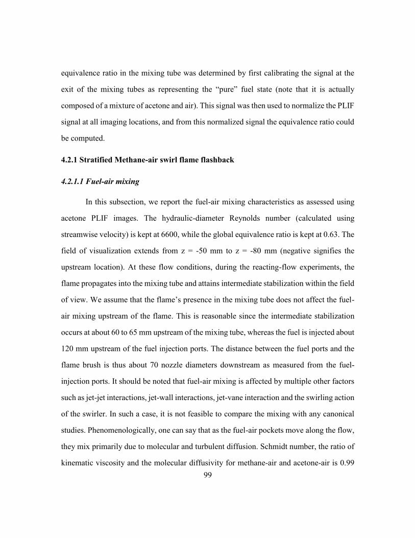
99
equivalence ratio in the mixing tube was determined by first calibrating the signal at the
exit of the mixing tubes as representing the “pure” fuel state (note that it is actually
composed of a mixture of acetone and air). This signal was then used to normalize the PLIF
signal at all imaging locations, and from this normalized signal the equivalence ratio could
be computed.
4.2.1 Stratified Methane-air swirl flame flashback
4.2.1.1 Fuel-air mixing
In this subsection, we report the fuel-air mixing characteristics as assessed using
acetone PLIF images. The hydraulic-diameter Reynolds number (calculated using
streamwise velocity) is kept at 6600, while the global equivalence ratio is kept at 0.63. The
field of visualization extends from z = -50 mm to z = -80 mm (negative signifies the
upstream location). At these flow conditions, during the reacting-flow experiments, the
flame propagates into the mixing tube and attains intermediate stabilization within the field
of view. We assume that the flame’s presence in the mixing tube does not affect the fuel-
air mixing upstream of the flame. This is reasonable since the intermediate stabilization
occurs at about 60 to 65 mm upstream of the mixing tube, whereas the fuel is injected about
120 mm upstream of the fuel injection ports. The distance between the fuel ports and the
flame brush is thus about 70 nozzle diameters downstream as measured from the fuel-
injection ports. It should be noted that fuel-air mixing is affected by multiple other factors
such as jet-jet interactions, jet-wall interactions, jet-vane interaction and the swirling action
of the swirler. In such a case, it is not feasible to compare the mixing with any canonical
studies. Phenomenologically, one can say that as the fuel-air pockets move along the flow,
they mix primarily due to molecular and turbulent diffusion. Schmidt number, the ratio of
kinematic viscosity and the molecular diffusivity for methane-air and acetone-air is 0.99

100
and 1.5, respectively. Thus, by keeping the same Re and similar Schmidt numbers, one
can argue that the mixing characteristics can be assessed reliably.
Figure 4-5 Instantaneous PLIF snapshots showing the distribution of equivalence ratio at
flashback-equivalent conditions. Reh = 6600
Figure 4-5 shows instantaneous statistically-uncorrelated PLIF images of fuel-air
mixing. The flow close to the center-body is predominantly fuel-lean. Stoichiometric and
fuel-rich pockets can be noticed in the flow close to the outer wall. This confirms that the

101
fuel-injection strategy of positioning the fuel-injection ports away from the center-body
leads to an inhomogeneous equivalence ratio distribution. The intermittent presence of
fuel-air pockets close to the center-body can be attributed to the swirl and turbulence in the
mixing tube flow.
Figure 4-6 shows the mean distribution of the equivalence ratio in the mixing tube.
At z = -80 mm, the equivalence ratio at the center-body is very lean (ϕ ~ 0.3) while the
flow at the outer wall is richer (ϕ ~ 0.9). The lean and rich flammability limits for methane-
air mixtures are 0.5 and 1.7 respectively, and near these limits the flame speed becomes
small. Thus, in a mean equivalence ratio field, the propagating flame would not be able to
reach z = -80 mm. At z = -68 mm there is a sudden change in the mean fuel-richness of the
flow, which can also be noted in the instantaneous PLIF images in Figure 4-5. The reason
behind it may be the orientation of the streamlines, which move out of the plane of the laser
sheet; thus, any fuel-rich pocket would move out of the measurement plane. The three-
dimensionality of the flow also makes it difficult to comment on the length-scales of the
fuel-air pockets.
Figure 4-6: Mean distribution of equivalence ratio during methane-air mixing at Reh =
6600, Global equivalence ratio = 0.63.
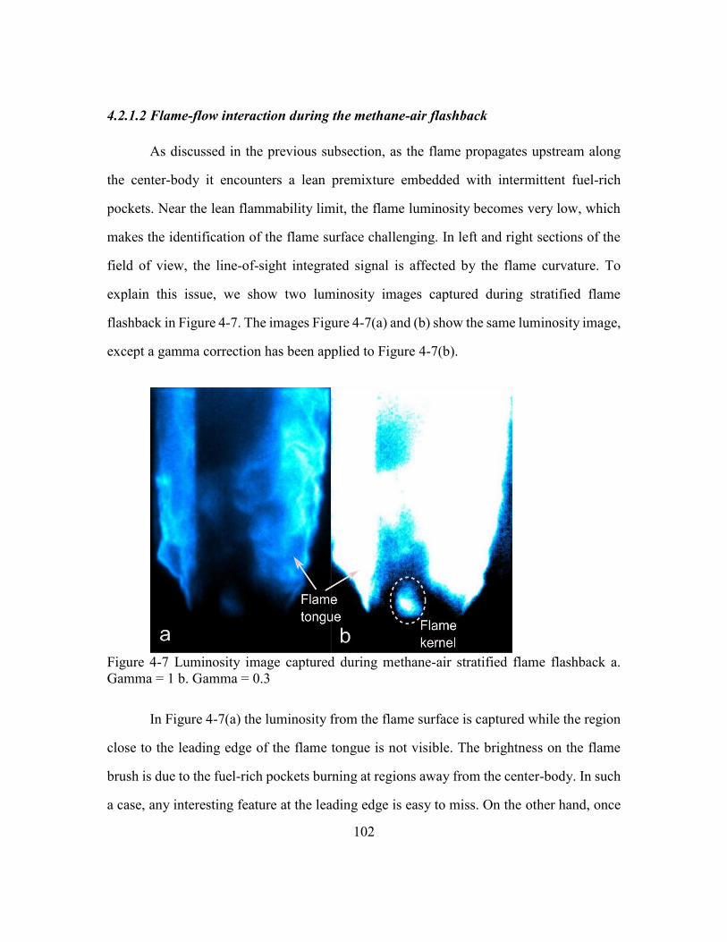
102
4.2.1.2 Flame-flow interaction during the methane-air flashback
As discussed in the previous subsection, as the flame propagates upstream along
the center-body it encounters a lean premixture embedded with intermittent fuel-rich
pockets. Near the lean flammability limit, the flame luminosity becomes very low, which
makes the identification of the flame surface challenging. In left and right sections of the
field of view, the line-of-sight integrated signal is affected by the flame curvature. To
explain this issue, we show two luminosity images captured during stratified flame
flashback in Figure 4-7. The images Figure 4-7(a) and (b) show the same luminosity image,
except a gamma correction has been applied to Figure 4-7(b).
Figure 4-7 Luminosity image captured during methane-air stratified flame flashback a.
Gamma = 1 b. Gamma = 0.3
In Figure 4-7(a) the luminosity from the flame surface is captured while the region
close to the leading edge of the flame tongue is not visible. The brightness on the flame
brush is due to the fuel-rich pockets burning at regions away from the center-body. In such
a case, any interesting feature at the leading edge is easy to miss. On the other hand, once

103
gamma is corrected to observe the leading line of the flame surface, we notice a flame
kernel near the flame front. It appears to be disconnected from the flame surface, but it
cannot be so, since the ignition of this kernel, which is at room temperature before burning,
is not possible without an ignition source. Any possibility of auto-ignition does not exist
since the fuel-air premixture is not preheated. This argument suggests that even though
there is nearly zero luminosity around the flame kernel, there should be a flame surface in
its vicinity that ignites it, as it moves downstream in the mixing tube. This raises the
question whether we can detect an ultra-lean flame that lies close to the center-body.
In this subsection, our discussion focuses on how the apparent flame kernels affect
the flame surface and the flow upstream of it. The leading regions of the flame surface –
in the absence of the fuel-rich pockets -- should play little role in blocking the approach
flow since the flame resides in barely-flammable lean regions. Hence, in the subsequent
paragraph, we discuss the interaction of the bright flame structures and approach flow.
Figure 4-8 shows the simultaneous luminosity and velocity fields upstream of the
flame surface. Figure 4-8(a) and Figure 4-8(b) are spaced by 3 ms while rest of the images
are captured 1 ms apart. Figure 4-8(b) – (d) tracks a bright flame structure, circled in
yellow, which crosses the laser sheet. The white region in the velocity contour plot
indicates the presence of flame products that vaporize the PIV seed particles. The effect of
the bright flame structure on the velocity field is evident as it crosses the laser sheet.
Regions of negative axial velocity are found upstream of the flame front during the time
that the structure crosses the laser sheet. Out-of-plane velocity (measured simultaneously
but not shown) is positive, which shows that these flame structures deflect the incoming
flow rather than causing flow reversal.
104
Figure 4-8 Chemiluminescence and the axial velocity fields at time instants: a. to, b. to +3,
c. to +4 and d. to +5 ms. Green line in the chemiluminescence images shows the position
of laser sheet. Evolution of a flame structure is marked by yellow circle.
Prior to the flame structure crossing the laser sheet, the planar profile of the flame
was not wrinkled. However, as noted in Figure 4-8(c) and (d), the flame kernel wrinkles
the flame surface and at the same time applies a strong blockage effect on the approach
flow. This structure imposes negative axial velocity on the approach flow. A similar
mechanism was found to assist the upstream propagation of the flame tongue in premixed
flame flashback [74],[57] However, for the case of stratified flame flashback, there is little
effect on the approach flow by the flame surface a bright flame structure appears. It should
also be noted that despite imposing very strong blockage effect on the approach flow, the
bright flame structure does not change its motion. Instead it keeps moving along its spiral
path towards the mixing tube exit. The apparent lack of deflection of the bright flame
structures’ path tells us that in global upstream motion of the flame brush during flashback,
a single flame kernel does not contribute to the propagation dynamically. Instead, it moves

105
along the spiral path around the center-body. Along its way out, the flame structure burns
out depending on its length scale. The burning out of this flame structure is identified by
the decrease in luminosity of the flame structure.
The chemiluminescence signal captured in these images are line-of-sight integrated
and have a strong dependence on local . A local variation in imposes variation in local
flame speed, stretches the flame surface and increases the flame curvature. The presence
of bright flame structures seems to result from the presence of locally fuel-rich pockets in
the flow, which is consistent with the non-reacting PLIF measurements. To confirm this
hypothesis, acetone PLIF measurements were taken for reacting flows as well. However,
seeding of fuel flow with acetone affected the flashback limits for a given bulk velocity
and required smaller fuel flow rates to trigger the flashback.
Figure 4-9 shows two normalized PLIF snapshots capturing the flame brush during
a stratified-flame flashback event. The flame front can be identified as the region of sharp
decrease in PLIF signal, which occurs owing to the pyrolysis of acetone in the preheat zone
of the flame. The regions of large curvature, such as the cusps (in red ellipse, Figure 4-
9(a)), are associated with a sharp change in the spatial distribution of . This observation
confirms the role of mixture variation in wrinkling of the flame brush of the flashing back
stratified flame; however, we are not able to map the PLIF signal to equivalence ratio owing
to pyrolysis and temperature variations that affect the acetone PLIF signal. Instead, the
pixel intensity was normalized with the maximum pixel value in the visualized region.
After normalization, the region with maximum PLIF signal should correspond to fuel-rich
regions. If we correspond these fuel-rich regions with those in the non-reacting flow, the
local equivalence ratio in these pockets should correspond to ~ 1.1-1.6 for the methane-
air mixture. As we discussed in the literature review, this range of equivalence ratio
corresponds to the unstretched laminar flame speed of 0.2 to 0.3 m/s. Thus the flame

106
wrinkling will occur depending on the local equivalence ratio gradient. If the pocket is
near-stoichiometric, it would induce positive curvature on the flame surface. On the other
hand, if the fuel-air pocket is near the flammability limits then the flame surface would
have little propagation in those regions. The resulting variation in local flame speed thus
modulates the flame surface. There should also be additional effects that come into play,
such as in a back-supported or front-supported flame environment, but these details are
difficult to comment upon.
Figure 4-9 Normalized acetone PLIF signal captured during the flashback
4.2.2 Stratified hydrogen-rich swirl flame flashback
Hydrogen-enrichment of fuel leads to new pathways for flames to propagate, as we
have discussed in section 4.1.3.2. In this section, we analyze hydrogen flashback behavior
for the case with the same mean axial velocity of 2.5 m/s and with hydrogen enrichment of
87% by mole. The global equivalence ratio is maintained at 0.4. First, we assess the mixing
behavior of the fuel and air.

107
4.2.2.1 Mixing behavior
Acetone PLIF was also used to investigate the mixing characteristics for the case
of stratified flashback with enriched-hydrogen fuel. However, in contrast to the work
above, the acetone was seeded into helium to create a non-reacting surrogate that had a
density that is closer to that of the enriched hydrogen fuel. Helium is seeded with acetone
by passing through the acetone bubbler. Instantaneous PLIF images for these runs is shown
in Figure 4-10.
A comparison of Figs. 4-5 and 4-10 indicates that the mixing behavior is
qualitatively similar to that of the methane-fuel case. There are fuel-lean yet locally-richer
fuel-air pockets spread across the mixing tube. The concentration and relative size of these
pockets are large close to the outer wall; however, there is an intermittent presence of fuel-
air pockets close to the center-body boundary layer.

108
Figure 4-10 Instantaneous equivalence ratio distribution during helium-air mixing Reh =
6300
The mean of 900 instantaneous images is shown in Figure 4-11. The mixing
behavior of the mean is also similar to that of methane-air mixing, except that the
equivalence ratio values are different. For the case of hydrogen-rich fuel, the equivalence
ratio does not reach stoichiometric in the mean, which simply reflects the lower global
equivalence ratio used. Also, instantaneously, there are pockets of near-stoichiometric
mixtures in the flow.

109
Figure 4-11 Mean equivalence ratio distribution in the mixing tube. Reh = 6300
The hydrogen-air mixture, even though fuel-lean in terms of equivalence ratio, is
still very reactive as compared to stoichiometric methane-air mixtures. The lean
flammability limit equivalence ratio for 87% hydrogen-methane mixture has a lower
flammability limit of 0.11. These limits encompass almost the entire visualized region in
the mixing tube. In flammable regions, the unstretched laminar flame speed of hydrogen-
air is as high as 3 m/s for near-stoichiometric fuel-air pockets. These fuel-air pockets occur
frequently in the regions close to the outer wall as shown in Figure 4-10, thereby increasing
the likeliness of flame propagation along the outer wall.
4.2.2.2 Time-resolved luminosity images and simultaneous PIV
We observe that hydrogen-rich flashback occurs in two steps. The first step is the
propagation along the center-body boundary layer in a way similar to that of the fully
premixed flame. The flame starts from a stable condition where it is anchored in the inner
shear layer of the combustor. Upon triggering the flashback, it propagates upstream
through the boundary layer of the center body. In a manner similar to the intermediate
stabilization, the flame tongue rotates around the center-body. The flame brush is broad

110
enough to maintain interaction with the outer wall. During this interaction, the flame
surface propagates to the outer wall and begins to propagate down it. It should be noted
that the flame’s existence along the outer wall is not favored by the swirling action since it
leads to the low-density fluid along the outer wall. The centrifugal force acts radially
outward and so the low-density gases on the outer wall is inherently unstable. Still, the
propagation of the flame surface along the outer wall occurs, primarily due to the fast
chemistry associated with the richer mixtures at the outer wall. In Figure 4-12 we show the
first definitive evidence of flame propagation along the outer wall using simultaneous time-
resolved PIV and luminosity. The framing rate for these measurements is 4 kHz.
Figure 4-12(a) shows an instant when the flame along the center-body and the outer
wall are on the either side of laser sheet (green). In 4.25 ms the flame on the center-body
revolves around the center-body and crosses the laser sheet. At the same time, the flame
structure on the outer wall also crosses the laser sheet in the opposite direction. At this
instant, the outer wall and the center-body flame structures share the same azimuthal
location. The propagation of the outer wall structure occurs as an acute flame tip shedding
the burnt gases as bright flame structures. The burnt gases, which are low in density, cannot
sustain themselves in the vicinity of the outer wall. Thus, immediately after getting burnt,
these gases form a puffy tail-like structure in the wake of the leading point of the
propagating flame surface. In Figure 4-12(c), the flame on the center-body has crossed the
laser sheet and is on the other side of the annulus. At this stage, the acute flame tip which
is anchored in the outer wall boundary layer, starts propagating upstream. During this
process, the single flame structure bifurcates into 2-3 flame structures approaching the fuel-
injection ports.

111
Figure 4-12 Chemiluminescence images and simultaneous axial velocity fields at different
time instances during flame propagation along the outer wall boundary layer. White region
in the velocity shows the burnt gas region.
While propagating, we expect the outer flame structure to apply blockage to the
approach flow. These flame structures, which push the approach flow in the negative
streamwise direction, can apply blockage to reverse the flow at the flame tip. To capture
this effect, the laser sheet needs to be imaged very close to the outer wall of the mixing
tube. The curvature of the mixing tube makes it difficult to capture this detail. In the results
reported here, we could get PIV data up to 2 mm away from the outer wall. Thus, any
portion of the flame and the flow within 2 mm of the wall could not be captured. However,
the blockage from the flame structure is apparent in Figure 4-12(d). Just upstream of the
flame tongue (z = -77 mm, r = 10.5 mm), the blockage effect from the flame reduces the
axial velocity to ~ 1 m/s, as marked by local light blue background.
Another interesting aspect of this propagation is the flame-flow interaction. The
flame structure on the center-body keeps swirling while anchored at an intermediate
location. This swirling flame can cause a sweeping effect in the azimuthal direction, similar
112
to the one discussed in previous chapter. On the other hand, the outer flame structure, which
is primarily controlled by the equivalence ratio distribution upstream of it, also interacts
with the flow by pushing in the opposite direction. Now, inside the mixing tube, these two
flames move in opposite swirling directions. The flow that is affected by the flame on the
center-body can also interact with the flame on the outer wall, which can cause a three-way
interaction. To ascertain this would require simultaneous multi-plane measurements which
was not possible with our current experimental setup.
To further understand the propagation along the outer wall, we describe the flame
propagation in two stages: (1) flame anchoring on the wall, and (2) flame advancement
along the wall. Flame anchoring on the wall can be defined by attachment of acute flame
tips on the outer wall. In this process, the flame does not move but resists getting convected
with the approach flow. At times, acute flame structures anchor themselves and thus resist
being convected by the upstream flow. The flame advancement stage starts when the flame
structure starts propagating upstream. In this phase, either the flame structure bifurcates
into two similar structures or it remains on the streaks of stoichiometric mixture (most
reactive mass fraction) and advances till the flameholding occurs.
PIV runs were conducted in an atmospheric-pressure burner with alumina seeding
particles. Alumina particles do not get consumed in the flame and so it is possible to obtain
velocity measurements in the burnt gas regions. In previous work, the 2D dilatation has
been found to agree well with the flame surface. [76],[78]. Theoretically, the three-
dimensional divergence value should be zero everywhere except for the flame surface.
Also, the larger the volume generation per unit volume, the larger would be the divergence.
Thus, it is also an indirect indicator of heat release, assuming that the entire heat release
acts to generate volume. With this idea, we use the 2D divergence value as the marker of

113
heat release. Another marker of heat release in stratified flows is luminosity, however
deriving any quantitative measurement is beyond the scope of current work.
Figure 4-13 shows two instants during the flame anchoring phase. At first there is
no acute structure on the wall, however a bright flame structure crosses the laser sheet
(shown with light green). In Figure 4-13(a), in the velocity field, the flame surface is
marked with a white line. Determination of the flame surface was accomplished by looking
for large changes in the local particle density [76],[79]. It can be noted that the flame
surface agrees well with the 2D dilatation, but only in the upstream portions of the flame
surface.
Previously reported work on fully premixed flame found these peaks of large 2D dilatation
all along the flame surface [53]. In Figure 4-13(b), even though the flame surface exists in
the laser sheet plane, there were no distinguishable peaks in the 2D dilatation map. One
can correlate the absence of bright flame structure in the laser sheet plane with the absence
of peaks in the 2D dilatation map. This observation agrees well with the idea that the bright
flame structures are associated with large heat release – and hence with large three-
dimensional dilatation which reflects in the 2D dilatation maps. With this argument, the
large 2D dilatation values at the upstream locations of the flame structure indicates that the
heat release on the flame structure is not the same all along the surface. The axially-
upstream side of the flame structures have larger dilatation than the axially-downstream
side of the flame tongue. This observation may be an outcome of the environment around
the propagating flame structure. These acute flame structures move through the stratified
fuel-air mixture, propagating along the regions of the most reacting mixture fraction. This
structure should have a relatively richer and a relatively leaner fuel air mixture on either
side of it. Hence, the sides of these structures – visualized as the axially upstream and
downstream side in Figure 4-13 should have different levels of dilatation. This should also

114
be reflected in the luminosity imaging; rich and lean sides of the flame structures should
have different levels of luminosity. However, no such evidence was found in the luminosity
images. Since, there is another dim flame structure in the background (revolving around
the center-body), any comment on the variation of luminosity across a flame structure is
difficult to make.
Figure 4-13 (a) Bright flame feature crossing the laser sheet and simultaneous 2D
divergence field, (b) Formation of acute tipped flame structure on the outer wall
In Figure 4-13(a), the bright flame structure in the luminosity image corresponds to
the region of high 2D dilatation in the PIV data. In Figure 4-13(b), the bright structure
115
moves downstream, while the acute-tipped flame structures stay as it is. In the PIV image
there is no sign of large dilatation in the vicinity of the flame surface.
For the flame advancement stage, we show three instantaneous PIV images along
with the luminosity (Figure 4-14). In these images, the flame surface exists along the
center-body boundary layer as well as along the outer wall. In Figure 4-14, the regions of
large divergence are associated with the flame on the center-body and not on the outer wall.
However, at subsequent times, this large divergence shifts toward the outer wall.
Simultaneously, the bright flame structure now interacts with the outer wall and assists in
making progress in the upstream direction.

116
Figure 4-14 Simultaneous luminosity images and 2D divergence maps. Regions of large
divergence correspond to the bright flame structures crossing the laser sheet.
If we associate the luminosity and the dilatation value with the heat release, these
bright flame structures are essentially sources of large heat release. Thus, when these
structures interact with the boundary layer, they allow the flame to anchor on the outer
wall. If they occur in tandem, or in the vicinity of the stoichiometric mixtures, they can
assist in upstream propagation of the flame.

117
4.2.3 Effect of elevated pressure
In the current study, elevated pressure flashback runs were conducted at the same
mean axial velocity as that of the atmospheric pressure runs. Thus, an increase in pressure
results in a proportional increase in the Reynolds number. In this work, we report flashback
behavior for methane-air stratified flames at 3 atm and Reh = 18,400. As in the atmospheric-
pressure cases, acetone PLIF was used to assess the fuel-air mixing behavior in the mixing
tube under non-reacting conditions. For example, Figure 4-15 shows instantaneous images
of equivalence ratio that were derived from the acetone PLIF data.
Figure 4-15. Instantaneous PLIF images showing the small-scale fuel-rich structures in the
flow. These images correspond to methane-air flashback at 3 atm. Reh = 18600 ϕg = 0.85
Pressure can affect flame propagation characteristics by affecting the reaction
chemistry and by increasing the turbulence through the higher Reynolds number. In our
discussion on stratified flame-flow interaction, pressure is likely to be important owing to
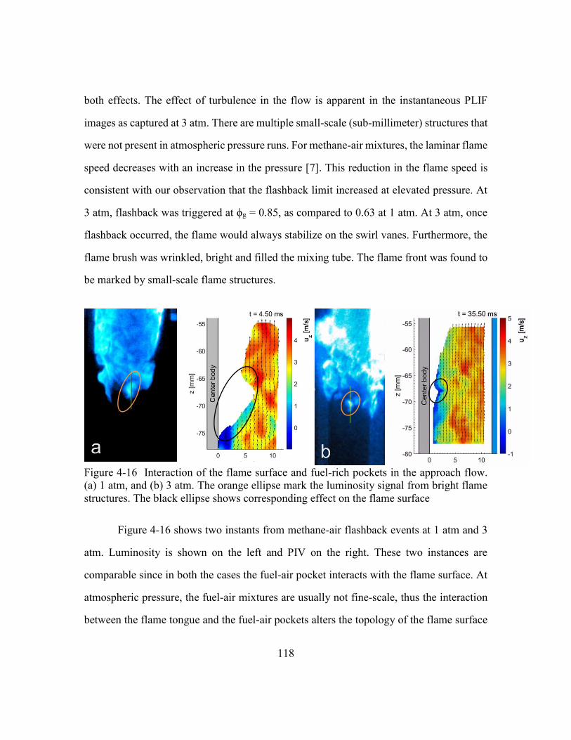
118
both effects. The effect of turbulence in the flow is apparent in the instantaneous PLIF
images as captured at 3 atm. There are multiple small-scale (sub-millimeter) structures that
were not present in atmospheric pressure runs. For methane-air mixtures, the laminar flame
speed decreases with an increase in the pressure [7]. This reduction in the flame speed is
consistent with our observation that the flashback limit increased at elevated pressure. At
3 atm, flashback was triggered at ϕg = 0.85, as compared to 0.63 at 1 atm. At 3 atm, once
flashback occurred, the flame would always stabilize on the swirl vanes. Furthermore, the
flame brush was wrinkled, bright and filled the mixing tube. The flame front was found to
be marked by small-scale flame structures.
Figure 4-16 Interaction of the flame surface and fuel-rich pockets in the approach flow.
(a) 1 atm, and (b) 3 atm. The orange ellipse mark the luminosity signal from bright flame
structures. The black ellipse shows corresponding effect on the flame surface
Figure 4-16 shows two instants from methane-air flashback events at 1 atm and 3
atm. Luminosity is shown on the left and PIV on the right. These two instances are
comparable since in both the cases the fuel-air pocket interacts with the flame surface. At
atmospheric pressure, the fuel-air mixtures are usually not fine-scale, thus the interaction
between the flame tongue and the fuel-air pockets alters the topology of the flame surface

119
significantly. It can be seen that these pockets can have a strong effect on the approach
flow as well. On the contrary, at 3 atm, the fuel-air pockets are smaller scale (red ellipse in
Figure 4-16(b)) and seem to have lower impact on the approach flow. Figure 4-16(b) shows
an instant at 3 atm when the rich fuel-air interacts with the flame surface. It is noted that
there was very little change to the flame surface (marked with black ellipse).
Elevated-pressure hydrogen rich flashback still follows the flashback behavior as
described for the atmospheric pressure case. Flashback experiments were conducted at 3
atm, with global equivalence ratio of 0.3. Hydrogen enrichment was kept at 86%. Similar
to the 1 atm case, the flame propagated along the center-body and then the flame switched
to the outer wall.
The propagation along the outer wall occurred in a similar way as that of at
atmospheric pressure; however, the flame along the outer wall was characterized as a wider
flame tongue, which is similar to observations of channel-flow flashback.
Figure 4-17 Luminosity images captured during hydrogen-rich flashback at 3 atm a. to b.
to + 12 ms c. to + 14 ms; Reh = 18600 ϕg = 0.3
120
Figure 4-17 shows three instants during a hydrogen-rich flashback event. In Figure
4-17(a) the flame brush clings to the outer wall of the mixing tube. Flame anchoring occurs
in a similar way as that of the 1 atm case. Two acute flame tips were found to propagate
along the outer wall in Figure 4-17(b). These acute tips are also a bit wider (by a few
millimeters). Interestingly the advancement towards the fuel injection ports occurs as a
wide band (10mm) instead of the acute-tipped flame feature. This suggests that the acute-
tip structures primarily anchor the flame in the outer wall boundary layer and act to spread
the flame in the approach flow such that a wide flame tongue could be formed.
Simultaneous PIV measurements could not be taken for elevated pressure measurements
due to limited number of experiments which could not capture the flame tongue
propagation within the field of visualization.
4.4 CONCLUSIONS
In this chapter, we analyzed the flame propagation behavior during stratified flame
flashback. The mean sense of stratification was kept in radial direction such that the regions
close to the center-body were fuel-lean, while the flow on the outer wall was fuel-rich. The
global equivalence ratio was kept at 0.63 and 0.85 for atmospheric and 3 atm methane-air
experiments respectively. For hydrogen-rich mixtures, the hydrogen-enrichment level was
kept at approximately 87% for atmospheric and elevated pressure experiments.
Multiple flashback runs were carried out to identify the flashback regime diagram
distinguishing the two modes of flame stabilization in the mixing tube, namely intermediate
stabilization and flame-holding. During intermediate stabilization of the flame, the
upstream propagating flame stops at an intermediate location in the mixing tube and keeps
swirling around the center body as a flame tongue with relatively-dim leading edge and
bright flame brush. It was noted that intermittently bright flame structures would appear at

121
the upstream edge of the flame and these structures would impose strong blockage on the
approach flow. However, these bright flame structure, which are rich fuel-air pockets in
the swirling, would merge with the flame brush without assisting towards the sustained
upstream movement of the flame along the center-body boundary layer. The flame leading
edge was dim in luminosity and did not seem to affect the upstream flow as strongly as a
fully premixed surface. The flame brush almost entirely filled the mixing tube during
intermediate stabilization of the flame.
The other mode of flame propagation, flameholding occurs when the flame
propagates along the outer wall boundary layer and anchors itself on the fuel ports. This
behavior was found prevalent in hydrogen-rich fuel. It was noted that the upstream
propagation of the flame initiates along the boundary layer of the center-body. As the flame
propagates upstream, it attains intermediate stabilization. Meanwhile, the flame brush
interacts with the fuel-rich pockets along the outer wall boundary layer. The bright flame
structures appear in the mixing tube, which upon interaction with the outer wall, anchor as
acute flame structures. These structures resist the approach flow and move slowly as seen
in lab-frame. However, these flame tip structures upon interacting with rich fuel-air pockets
start propagating along the outer wall and keep progressing until the flame-holding
happens. The bright flame structures which assist in upstream propagation are found to
concur with strong 2D dilatation in the velocity field. This suggests that these flame
structure impose strong blockage on the approach flow, thereby assisting in the acute-tip
flame anchoring.
These two modes of flame propagation were found to occur at elevated pressures
as well. Although flashback experiments were conducted up to 5 atm (Reh ~ 33000) for
flashback regime determination, elevated pressure high-speed laser diagnostic was carried
out only up to 3 atm (Reh ~ 18300). It was noted that the nature of flame-flow interaction

122
for methane-air flames stayed the same. The flame surface stabilized itself at an
intermediate location in the mixing tube. The finer scale fuel-air pockets were found to
appear at the region immediately upstream of the flame tongue. These fuel-air pockets did
not affect the flow field at elevated pressure as strongly as during the atmospheric pressure
flashback experiments.
For hydrogen-rich fuel at elevated pressure, the flame-holding started with
interaction of bright flame structures with the outer wall. Acute flame structures were found
to anchor in the turbulent boundary layer on the outer wall. After flame anchoring, a wide
flame tongue was found to form during the flame advancement stage. The appearance and
propagation behavior of the flashback was similar to that of channel flashback.
123
CHAPTER 5 : SUMMARY AND FUTURE WORK
The research work in this thesis is aimed towards improving the current
understanding of boundary layer flashback with the use of high-speed imaging and laser
diagnostics. The focus of this study was on the upstream flame propagation mechanisms
under fully premixed and stratified conditions. The experiments were conducted in an
optically accessible annular swirl combustor, which allowed for flow imaging inside the
mixing tube. For the elevated-pressure flashback experiments, a back-pressure-controlled
combustion facility was designed ab-initio and installed at the J.J. Pickle Research Campus
at UT Austin. For the stratified flame experiments, a swirl-nozzle design was used that was
inspired by fuel-injection methods used in some industrial gas-turbine combustors. In this
design the fuel is injected into the main swirling flow through fuel ports in the swirler
vanes. These fuel ports were located close to the outer wall such that stratification is
achieved in the radial direction. Flashback experiments were conducted at pressures up to
5 atm. Hydrogen-enrichment level in the methane-hydrogen fuel was varied from 0% to
87% by volume. The mean axial velocity was kept at 1.0 – 4.0 m/s for flashback runs;
however, the laser diagnostic experiments were carried out at the mean axial velocity of
2.5 m/s. By varying the chamber pressure, the hydraulic-diameter-based Reynolds number
was varied from 2×10³ to 3.3×10⁴. A kHz-frame-rate imaging system equipped with a
high-speed image-intensifier was used to capture time-resolved chemiluminescence
images and simultaneous three-component particle image velocimetry (PIV) data. The
assessment of fuel-air mixing was carried out by seeding acetone vapor into the fuel stream
and imaging its distribution using planar laser induced fluorescence.
The main objective of this work was to understand the flame-flow interaction
during swirl flame flashback. For this, we first investigated fully-premixed flashback and
analyzed the effect of three-dimensionality of the flame-flow interaction on the flame

124
propagation behavior. Upon developing the three-dimensional picture of the propagating
flame, further work was focused on flashback that occurs in stratified pre-mixtures. Global
flame propagation and stabilization behavior for a stratified swirl flame is reported in this
work. High-speed diagnostics were used to investigate the flame propagation behavior, and
two different modes of flame propagation were identified. In the following paragraphs, I
summarize the findings of this thesis work and propose future work.
5.1 Three-dimensional picture of premixed swirl flame flashback
This work extended the data analysis performed in [76][55], to reveal new physics
of flame-flow interaction during flashback in premixed reactants. In this new method for
swirling flows, planar 3-component time-resolved PIV data were used to create space-time
reconstructions of the 3D flow-field. Focus was kept on low-turbulence stoichiometric
methane-air flames since the appearance of this flame is smooth and the global propagation
behavior is stable. The most upstream point of the flame, the flame tip, was tracked using
the time-resolved luminosity images. It was demonstrated that the flame tip moves with a
nearly-constant angular and axial velocity during upstream propagation in the mixing tube.
[47]. It was also noted that the flame surface topological features such as the leading edge
and the flame tip retain their shapes and sizes during upstream propagation. Based on this
observation, a hypothesis of frozen-flame surface was made. This hypothesis imposes the
constancy of flame surface in strict sense. The simultaneity of luminosity images and
planar information in the laser sheet plane, allowed us to employ space-time equivalence.
Under this assumption, the planar images captured in a time-resolved manner were stacked
in space such that a three-dimensional flow-field was created. This method also enabled
the reconstruction of the 3D flame surface. The reconstructed flame surface and the
luminosity images of methane-air flashback were found to be in excellent agreement,
125
which offers some level of validation of the methodology. The flame surface reconstruction
revealed the details on the surface such as the curved flame leading edge or the wrinkles
on the flame surface; however, a detailed characterization of the flame surface was not the
focus of this work.
The reconstruction of the velocity field provided the flow field in an annulus sector
volume, which is a challenging view to obtain with alternative experimental techniques
such as tomographic PIV. The three-dimensional quasi-instantaneous flame surface and
flow field provided a detailed picture of swirling flame and flow interaction. Quasi-
streamlines in the upstream flow were drawn and it was revealed that the flame surface
deflects the approach flow in all three directions. In earlier research, attention had been
paid to the flame surface blocking the approach flow in the z-direction (along the axis of
the center-body). For the first time, the blockage effect of the flame surface was shown to
disturb the velocity field in all three directions. This demonstrated blockage effect indicates
the presence of a substantial pressure gradient in the vicinity of the flame front. The
pressure gradient is often cited as the reason for baroclinic vorticity generation at the flame
surface.
Further analysis of the flame-flow interaction was carried out by shifting the
reference frame to that of the moving flame surface. This change in observer’s frame
allowed the flame surface to be steady in time. This approach conveniently allowed us to
recreate a steady-flow picture of flame-flow interaction. Once the steady flow-field and
flame surface was obtained, the kinematics of a fluid particle could be analyzed before and
after burning. In the unburnt section the fluid particle is shown to deflect radially outward
upon approaching the flame surface. In the burnt gases, the fluid particle was found to
deflect radially inward towards the center-body surface. This observation is not in

126
agreement with the current understanding of flashback in 2D channels, hence an analysis
of fluid parcel movement was carried out with fundamental Newtonian mechanics.
Application of Newtonian mechanics is valid only for inertial frames, i.e., frames
which are non-accelerating in nature. The flame structure moves with a constant axial and
angular velocity; hence the rotation of the flame structure makes it an accelerating frame
of reference. To apply Newtonian mechanics in an accelerating frame of reference, inertial
forces or fictitious forces need to be considered. This brings in the role of centrifugal and
Coriolis forces in flame-flow interaction. It was assumed that viscous forces have limited
role in the kinematics of the fluid parcel. Hence, the motion of the particle can be explained
from the balance of three forces, pressure-gradient, centrifugal and Coriolis. By definition,
the Coriolis force on a fluid particle depends on the relative velocity of the approaching
fluid parcel. On the other hand, for any kind of flashback, it has been shown that the
approach flow speed changes due to the blockage effect from the flame surface. Thus, in a
rotating frame, the blockage from the flame affects the Coriolis force acting on the fluid
particle. The radial component of the Coriolis force is particularly affected by the swirling
flame thereby disturbing the force-acceleration balance in the radial direction. It is shown
that the Coriolis force experiences a quick increase when the particle crosses the flame
surface and accelerates. The resulting force in the radially inward direction concurs with
the radial deflection of the fluid particle. However, this motion can not be entirely ascribed
to the Coriolis action since the pressure field remains unknown. We further show that the
pressure field estimation can not be carried out from a quasi-reconstructed velocity field,
owing to the lack of precision.

127
5.1.1 FUTURE WORK ON PREMIXED-FLAME FLASHBACK
There are several aspects from this work which could be studied further in future. The
frozen flame assumption has allowed us to recreate the flame surface of a propagating
flame feature. This could be used to obtain detailed information of the flame surface
curvature of propagating flames, which could be helpful in assessing fundamental
quantities such as flame stretch. Another direction for future studies would be to understand
the flashback from the flame’s frame of reference. The prevalent approach of predicting
the flashback propensity is by identifying the low-momentum approach flow regions, such
as in the boundary layer. The closer the flame is to the wall, the more likely it is to
flashback. However, while looking at the approach flow from swirl flames’ reference
frame, the low momentum zone does not exist near the wall but at a certain length away
from the wall. The presence of a low momentum zone away from the wall implies that the
possibility of flame quenching would be low in such a case. Any investigation in this
research direction could also explain the larger flashback propensity of swirling flames
relative to non-swirling ones.
5.2 Stratified flame flashback
In next part of this thesis, stratified flame experiments were conducted for a wide
range of Reynolds numbers. The level of hydrogen enrichment was varied up to 87%. The
global propagation behavior of the flame tongue was studied and two modes of flame
stabilization in the mixing tube. The first mode, intermediate stabilization, corresponded
to the case when the propagating flame stops at an intermediate location in the mixing tube,
and keeps swirling without making a continuous upstream movement. The overall
appearance of the flame surface was characterized with a bright flame brush and a relatively
dim upstream flame surface. At the leading side of the flame tongue, intermittent bright

128
structures were noted. The second mode of flame stabilization is characterized by the
anchoring of the flame on the fuel ports. In this mode, the flame propagation occurs along
the outer wall and it continues until the flame is stabilized on the fuel ports.
The assessment of the degree of stratification was carried out in non-reacting flows
with planar laser-induced fluorescence (PLIF) of acetone seeded into the “fuel” stream.
The instantaneous PLIF images revealed the distribution of equivalence ratio in the flow
field. It was noted that the fuel-rich pockets are frequent near the outer wall, but there is an
intermittent presence of these pockets near the center-body. In the mean sense, the flow
near the outer wall is richer (ϕ ~ 1.0-1.5 for methane, ϕ ~ 0.5 – 0.6 for hydrogen) than near
the center-body. These equivalence ratios correspond to unstretched laminar flame speeds
as high as 0.30 m/s and 1.5 m/s for methane and hydrogen, respectively. In an instantaneous
sense, the maximum equivalence ratios were higher for both methane and hydrogen, which
corresponded to maximum unstretched laminar flame speeds of 0.30 m/s and 3.0 m/s. Thus,
in an instantaneous sense, a hydrogen-air flame has faster propagation speed by an order
of magnitude.
Simultaneous high-speed luminosity imaging and stereoscopic PIV measurements
were captured at 4 kHz. In the intermediate stabilization mode, it was observed that there
are bright flame structures near the leading edge of the flame, which grow in time until
they merge with the flame brush. These flame structures seem to follow the path of the
swirling flow, which indicates that the effect of flame tongue’s blockage is not a dominant
factor in flame-flow interaction. Instead, it is noted that the bright flame structures impose
strong blockage on the approach flow. However this blockage is not sustained in time, thus
any assistance in upstream propagation of flame is not available. The case of hydrogen-
rich flame is different though.

129
The flame profile captured in the laser sheet plane confirmed the presence of flame
structure on the outer wall during hydrogen-rich flashback. The simultaneous luminosity
imaging revealed the presence of acute-tipped flame structures on the outer wall. The outer
wall propagation of the flame occurred in two distinct phases. In the first phase, the
formation of the acute-tipped flame structure initiates upon interaction of bright flame
structures with the outer wall. In this phase, the flame structure resists the approach flow
without moving in the axial or azimuthal direction. The next phase is marked with the flame
advancement towards the fuel ports. In this phase, the flame tip catches on to near
stoichiometric mixtures along the outer wall. The flame structure gets brighter as it
approaches the fuel ports.
The elevated pressure experiments revealed the role of turbulence in breaking the
fuel-parcels into smaller fuel rich pockets. These fuel rich pockets appear as bright flame
structures at the leading edge of the flame tongue, however the sizes of bright flame
structure are millimeter scale. This flame structure does not affect the flow as much as its
atmospheric pressure counterpart. For elevated-pressure hydrogen-rich flashback, the
mechanism of acute flame anchoring was the same as that of atmospheric pressure
flashback. However, at the flame advancement stage, the flame propagated as a wide flame
brush along the outer wall.
5.2.1 FUTURE WORK ON STRATIFIED-FLAME FLASHBACK
Future studies in understanding the stratified flame flashback should be directed
towards getting the instantaneous three-dimensional distribution of equivalence ratio. With
the current know-how, it would a challenging experiment in the confined space of the
mixing tube. An achievable target would be to get the time-resolved PLIF data inside the
130
mixing tube, which would allow us to understand the three-dimensional correlated features
in the fuel-air pockets. By doing so, one could predict how the fuel-rich pockets would
burn. A simultaneous tomographic PIV data could further help us in elucidating the role of
back-supported/front-supported mechanism on the flame propagation during flashback.
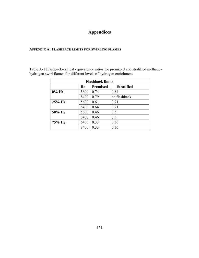
131
Appendices
APPENDIX A: FLASHBACK LIMITS FOR SWIRLING FLAMES
Table A-1 Flashback-critical equivalence ratios for premixed and stratified methane-
hydrogen swirl flames for different levels of hydrogen enrichment
Flashback limits
Re Premixed Stratified
0% H2 5600 0.74 0.84
8400 0.79 no flashback
25% H2 5600 0.61 0.71
8400 0.64 0.71
50% H2 5600 0.46 0.5
8400 0.46 0.5
75% H2 6400 0.33 0.36
8400 0.33 0.36

132
APPENDIX B: MATHEMATICAL FORMULATION OF FROZEN FLAME ASSUMPTION
A parametric expression for a three-dimensionally curved surface can be written as
𝑆(𝑡) = 𝑥(𝑡)𝑖̂ + 𝑦(𝑡)𝑗̂ + 𝑧(𝑡)�̂�
where, x,y and z refer to the cartesian coordinates. While 𝑖̂, 𝑗̂, �̂� refer to the unit vectors. 𝑡
represents time variable. Since the surface is moving in space, the coordinates are time-
dependent.
In cylindrical coordinates, this expression can be written as
𝑆(𝑡) = 𝑟(𝑡)�̂�𝑟 + 𝜃(𝑡)�̂�𝜃 + 𝑧(𝑡)�̂�
where 𝑟, θ 𝑎𝑛𝑑 𝑧 represent the radial, azimuthal and axial coordinates
Initially, at 𝑡 = 𝑡0, let us say that the surface is represented as 𝑆0.
Then, at time, 𝑡 = 𝑡0 + 𝛥𝑡
𝑆(𝑡0 + 𝛥𝑡) = 𝑟(𝑡0 + 𝛥𝑡)�̂�𝑟 + 𝜃(𝑡0 + 𝛥𝑡)�̂�𝜃 + 𝑧(𝑡0 + 𝛥𝑡)�̂�
133
Under frozen flame assumption, the back-pressure supported flame surface moves like a
solid surface for a small 𝛥𝑡. For current analysis, there is only swirling and axial motion
of the flame surface. Thus,
𝑟(𝑡0 + 𝛥𝑡) = 𝑟(𝑡0)
𝜃(𝑡0 + 𝛥𝑡) = 𝜃(𝑡0) + 𝛺𝑓𝛥𝑡
𝑧(𝑡0 + 𝛥𝑡) = 𝑧(𝑡0) + 𝑣𝑧,𝑓𝛥𝑡
where, 𝛺𝑓 and 𝑣𝑧,𝑓 represent the velocity of the flame tip (or tongue). It should be noted
that these expressions can be extended to higher-order terms of a Taylor series expansion,
however for the current set of measurements and experiments, it is not done.
𝑆(𝑡0 + 𝛥𝑡) = 𝑆0 + 𝛺𝑓𝛥𝑡 �̂�𝜃 + 𝑣𝑧,𝑓𝛥𝑡 �̂�
Relative to any observer moving in the lab-frame with a velocity 𝑣 𝑜𝑏𝑠 = 𝑣𝑜𝑏𝑠,𝑟�̂�𝑟 +
𝛺𝑜𝑏𝑠�̂�𝜃 + 𝑣𝑜𝑏𝑠,𝑧�̂�, the equation for the surface is expressed by
𝑆(𝑡0 + 𝛥𝑡) = 𝑆0 + (𝛺𝑓 − 𝛺𝑜𝑏𝑠)𝛥𝑡 �̂�𝜃 + (𝑣𝑧,𝑓 − 𝑣𝑜𝑏𝑠,𝑧)𝛥𝑡 �̂�
Thus, for an observer co-rotating with the flame, surface coordinates become independent
of time
134
𝑆(𝑡0 + 𝛥𝑡) = 𝑆0 + (𝛺𝑓 − 𝛺𝑜𝑏𝑠)𝛥𝑡 �̂�𝜃 + (𝑣𝑧,𝑓 − 𝑣𝑜𝑏𝑠,𝑧)𝛥𝑡 �̂�
Let us define the laser sheet plane
𝐿 = 𝑟(𝑡)�̂�𝑟 + 𝜃(𝑡)�̂�𝜃 + 𝑧(𝑡)�̂�
Since the laser sheet is aligned along the radial-axial place, azimuthal position of the laser
sheet is fixed in lab-frame. Hence, the laser sheet can be expressed as
𝐿 = 𝑟�̂�𝑟 + 𝜃0�̂�𝜃 + 𝑧�̂�
It should be noted that the expression for L represents the set of points in the laser sheet
plane. Thus, the vectorial components do not represent the surface normal but the
position vectors of points in the plane. There is no temporal dependence in the laser sheet
location in lab-frame. However, for an observer co-moving with the flame, the relative
position of the laser sheet changes.
𝐿𝑠ℎ𝑒𝑒𝑡,𝑓 = 𝑟�̂�𝑟 + (𝜃0 − 𝛺𝑓𝛥𝑡)�̂�𝜃 + (𝑧 − 𝑣𝑧,𝑓𝛥𝑡)�̂�

135
For an observer in lab-frame when the flame surface crosses the laser sheet, the flame
profile as captured in the laser sheet is an intersection of the flame surface and the laser
sheet. Thus, the flame profile (𝑃𝑓𝑙) can be expressed as
𝑃𝑓𝑙 = 𝑆ꓵ𝐿
Since, at least one of the two surfaces is moving, irrespective of the observers frame, the
plane profile changes with time and space. It can be expressed as
𝑃𝑓𝑙 = 𝑆(𝑡)ꓵ𝐿⏟ 𝐼𝑛 𝑙𝑎𝑏−𝑓𝑟𝑎𝑚𝑒
= 𝑆ꓵ𝐿(𝑡)⏟ 𝐼𝑛 𝑓𝑙𝑎𝑚𝑒−𝑓𝑟𝑎𝑚𝑒
This equation marks an important implication of the frozen flame. The flame profiles
obtained in the laser sheet by a lab-frame observer, are the same as the flame profiles
captured by moving the laser sheet, as is seen by a flame-frame observer. Thus, if we
know the relative position of the laser sheet in the flame-frame, we can reconstruct the
three-dimensional flame surface, as one would do with a scanning-laser sheet.

136
APPENDIX C: ASSEMBLY DRAWINGS OF THE PRESSURE CHAMBER
Figure C-1 Assembly of the central section of the pressure chamber
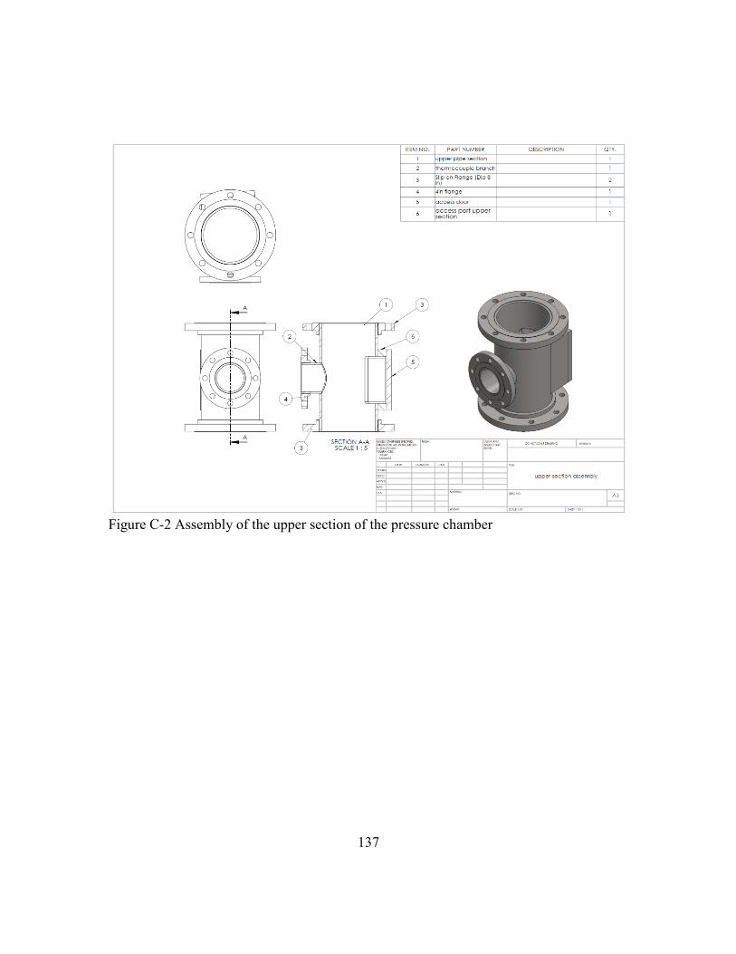
137
Figure C-2 Assembly of the upper section of the pressure chamber
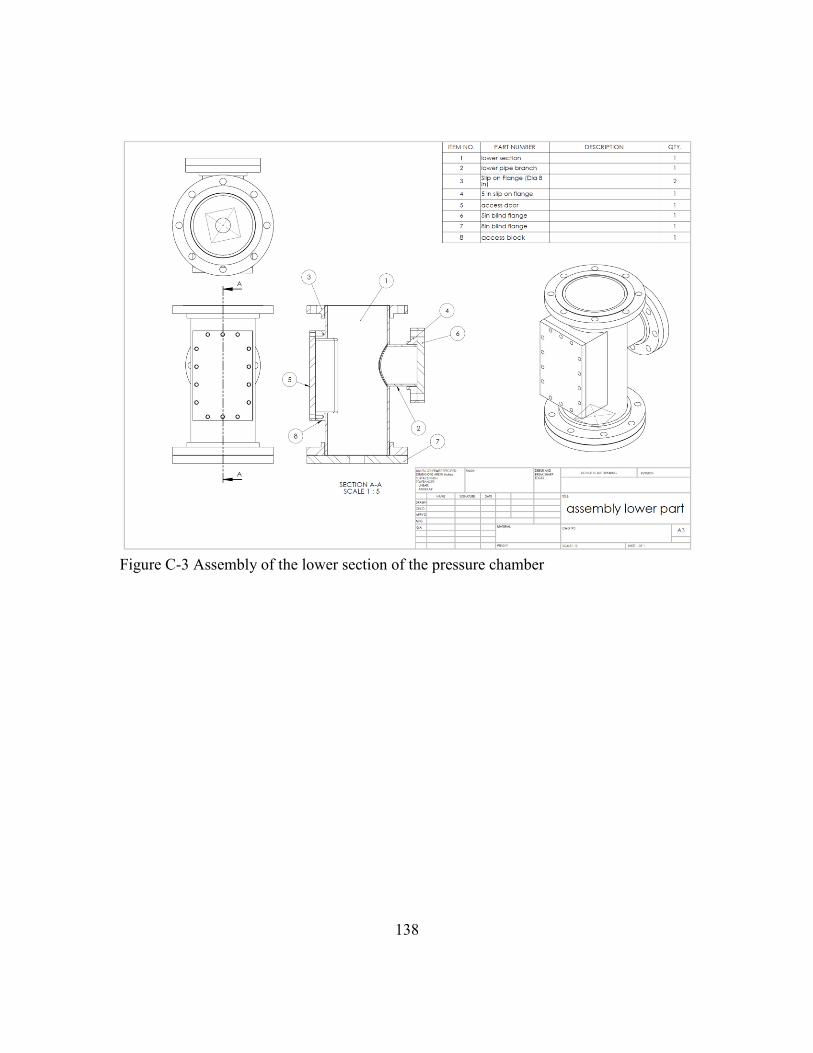
138
Figure C-3 Assembly of the lower section of the pressure chamber
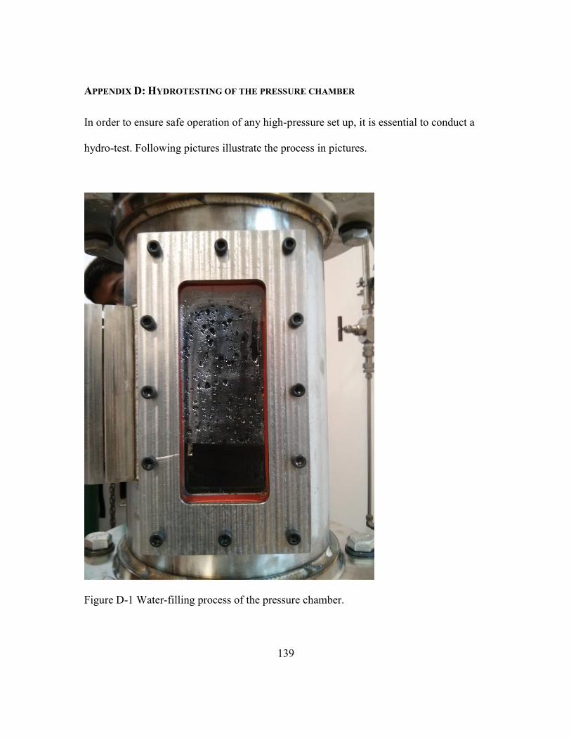
139
APPENDIX D: HYDROTESTING OF THE PRESSURE CHAMBER
In order to ensure safe operation of any high-pressure set up, it is essential to conduct a
hydro-test. Following pictures illustrate the process in pictures.
Figure D-1 Water-filling process of the pressure chamber.

140
First, the pressure chamber was isolated from the upstream and downstream piping.
Thereafter, tap-water was supplied to the chamber using a rubber hose which was
connected to the top-flange of the chamber. The water level was continuously gauged
during the filling process, as illustrated in Fig. D-1. Once the water filling was done, the
top flange nuts were also tightened. A quarter-inch Swagelok connection was provided at
the top in order to supply high-pressure air. A pressure gauge was mounted on the top
flange, as shown in Fig D-2. Once the desired pressure (100 psig) was reached the air
supply to the chamber was discontinued.
Figure D-2 Air supply and pressure monitoring at the top flange of the chamber

141
The pressure reading was continuously monitored. During pressurized condition, any
possible leaks were tended to. After confirming that the air pressure stayed the same for
over an hour, the hydro-test of the pressure chamber was deemed successful.
Figure D-3 General arrangement of the set up during pressurized condition

142
References
[1] V. G. Mcdonell, “3.1-1 Key Combustion Issues Associated with Syngas and High-
Hydrogen Fuels , The Gas Turbine Handbook, NETL 2006
[2] T. Lieuwen, V. Mcdonell, E. Petersen, and D. Santavicca, “Fuel Flexibility
Influences on Premixed Combustor Blowout, Flashback, Autoignition, and
Stability.”
[3] T. Lieuwen, V. McDonell, D. Santavicca, and T. Sattelmayer, “Burner
Development and Operability Issues Associated with Steady Flowing Syngas Fired
Combustors,” Combust. Sci. Technol., vol. 180, no. 6, pp. 1169–1192, May 2008.
[4] J. and B. A. Meher-Homji, C. Zachary, “Gas turbine fuel system design.
Combustion and operability,” Proc. Thirty-Ninth Turbomach. Symp., 2010.
[5] B. Lewis and G. von Elbe, “Stability and Structure of Burner Flames,” J. Chem.
Phys., vol. 11, no. 2, p. 75, 1943.
[6] A. Kalantari and V. McDonell, “Boundary layer flashback of non-swirling
premixed flames: Mechanisms, fundamental research, and recent advances,” Prog.
Energy Combust. Sci., vol. 61, pp. 249–292, 2017.
[7] C. K. Law, Combustion Physics. Cambridge: Cambridge University Press, 2006.
[8] Andrei Lipatnikov, Fundamentals of Premixed Turbulent Combustion - Andrei
Lipatnikov - Google Books. 2012.
[9] D. Shimokuri and S. Ishizuka, “Flame stabilization with a tubular flame,” Proc.
Combust. Inst., vol. 30, no. 1, pp. 399–406, Jan. 2005.
[10] B. Lautrup, Physics of Continuous Matter: Exotic and Everyday Phenomena in the
Macroscopic World. 2011.
[11] S. Ishizuka, “Characteristics of tubular flames,” Prog. Energy Combust. Sci., vol.
19, no. 3, pp. 187–226, Jan. 1993.
[12] A. Schönborn, P. Sayad, and J. Klingmann, “Influence of precessing vortex core
on flame flashback in swirling hydrogen flames,” Int. J. Hydrogen Energy, vol. 39,
no. 35, pp. 20233–20241, 2014.
[13] P. Sayad, A. Schönborn, M. Li, and J. Klingmann, “Visualization of Different
Flashback Mechanisms for H 2 /CH 4 Mixtures in a Variable-Swirl Burner,” J.
Eng. Gas Turbines Power, vol. 137, no. 3, p. 31507, Oct. 2014.
[14] H. Kröger, N. Kornev, D. Wendig, and E. Hassel, “Premixed flame propagation in
a free straight vortex,” Forsch. im Ingenieurwes., vol. 72, no. 2, pp. 85–92, Jun.
2008.
[15] Ishizuka, “Flame propagation along the vortex flows.”
[16] S. Ishizuka, “Flame propagation along a vortex axis,” vol. 28, pp. 477–542, 2002.
[17] T. Hasegawa, S. Michikami, T. Nomura, D. Gotoh, and T. Sato, “Flame
development along a straight vortex,” Combust. Flame, vol. 129, no. 3, pp. 294–
304, 2002.
[18] J. Chomiak, “Dissipation fluctuations and the structure and propagation of

143
turbulent flames in premixed gases at high reynolds numbers,” Symp. Combust.,
vol. 16, no. 1, pp. 1665–1673, Jan. 1977.
[19] W. T. ASHURST, “Flame Propagation Along a Vortex: the Baroclinic Push,”
Combust. Sci. Technol., vol. 112, no. 1, pp. 175–185, Jan. 1996.
[20] F. Kiesewetter, M. Konle, and T. Sattelmayer, “Analysis of Combustion Induced
Vortex Breakdown Driven Flame Flashback in a Premix Burner With Cylindrical
Mixing Zone,” J. Eng. Gas Turbines Power, vol. 129, no. October 2007, p. 929,
2007.
[21] C. Heeger, R. L. Gordon, M. J. Tummers, T. Sattelmayer, and A. Dreizler,
“Experimental analysis of flashback in lean premixed swirling flames: upstream
flame propagation,” Exp. Fluids, vol. 49, no. 4, pp. 853–863, Oct. 2010.
[22] R. W. Bilger, S. B. Pope, K. N. C. Bray, and J. F. Driscoll, “Paradigms in turbulent
combustion research,” Proc. Combust. Inst., vol. 30, no. 1, pp. 21–42, 2005.
[23] J. F. Driscoll, “Turbulent premixed combustion: Flamelet structure and its effect
on turbulent burning velocities,” Progress in Energy and Combustion Science, vol.
34, no. 1. pp. 91–134, 2008.
[24] P. Venkateswaran, A. Marshall, J. Seitzman, and T. Lieuwen, “Scaling turbulent
flame speeds of negative Markstein length fuel blends using leading points
concepts,” Combust. Flame, vol. 162, no. 2, pp. 375–387, Feb. 2015.
[25] B. E. Milton and J. C. Keck, “Laminar Burning Velocities in Stoichiometric
Hydrogen and Hydrogen-Hydrocarbon Gas Mixtures.”
[26] G. Yu, C. K. Law, and C. K. Wu, “Laminar flame speeds of hydrocarbon + air
mixtures with hydrogen addition,” Combust. Flame, vol. 63, no. 3, pp. 339–347,
Mar. 1986.
[27] V. Di Sarli and A. Di Benedetto, “Laminar burning velocity of hydrogen–
methane/air premixed flames,” Int. J. Hydrogen Energy, vol. 32, no. 5, pp. 637–
646, Apr. 2007.
[28] E. Hu, Z. Huang, J. He, C. Jin, and J. Zheng, “Experimental and numerical study
on laminar burning characteristics of premixed methane–hydrogen–air flames,”
Int. J. Hydrogen Energy, vol. 34, no. 11, pp. 4876–4888, Jun. 2009.
[29] J. Wang, Z. Huang, C. Tang, H. Miao, and X. Wang, “Author’s personal copy
Numerical study of the effect of hydrogen addition on methane–air mixtures
combustion,” 2008.
[30] Q. Li, G. Hu, S. Liao, Q. Cheng, C. Zhang, and C. Yuan, “Kinetic Effects of
Hydrogen Addition on the Thermal Characteristics of Methane−Air Premixed
Flames.”
[31] E. Hu, Z. Huang, J. He, and H. Miao, “Experimental and numerical study on lean
premixed methane–hydrogen–air flames at elevated pressures and temperatures,”
Int. J. Hydrogen Energy, vol. 34, no. 16, pp. 6951–6960, Aug. 2009.
[32] A E Dahoe, “Laminar burning velocities of hydrogen–air mixtures from closed
vessel gas explosions,” J. Loss Prev. Process Ind., vol. 18, pp. 152–166, 2005.
[33] F. Halter, C. Chauveau, N. Djebali-Chaumeix, and I. Gökalp, “Characterization of
the effects of pressure and hydrogen concentration on laminar burning velocities of
144
methane–hydrogen–air mixtures,” Proc. Combust. Inst., vol. 30, pp. 201–208,
2005.
[34] X. J. Gu, M. Z. Haq, M. Lawes, and R. Woolley, “Laminar Burning Velocity and
Markstein Lengths of Methane–Air Mixtures,” Combust. Flame, vol. 121, pp. 41–
58, 2000.
[35] V. Moccia and J. D’Alessio, “Burning behaviour of high-pressure CH4-H2-air
mixtures,” Energies, vol. 6, no. 1, pp. 97–116, 2013.
[36] A. E. Dahoe, “Laminar burning velocities of hydrogen–air mixtures from closed
vessel gas explosions,” J. Loss Prev. Process Ind., vol. 18, no. 3, pp. 152–166,
May 2005.
[37] T. Iijima and T. Takeno, “Effects of temperature and pressure on burning
velocity,” Combust. Flame, vol. 65, no. 1, pp. 35–43, Jul. 1986.
[38] E. Salzano, F. Cammarota, A. Di Benedetto, and V. Di Sarli, “Explosion behavior
of hydrogen-methane/air mixtures,” J. Loss Prev. Process Ind., vol. 25, no. 3, pp.
443–447, 2012.
[39] Y. Mizobuchi, J. Shinjo, S. Ogawa, and T. Takeno, “A numerical study on the
formation of diffusion flame islands in a turbulent hydrogen jet lifted flame,” Proc.
Combust. Inst., vol. 30, no. 1, pp. 611–619, Jan. 2005.
[40] A. Pires Da Cruz, A. M. Dean, and J. M. Grenda, “A numerical study of the
laminar flame speed of stratified methane/air flames,” Proc. Combust. Inst., vol.
28, no. 2, pp. 1925–1932, 2000.
[41] A. R. Masri, “Partial premixing and stratification in turbulent flames,” Proc.
Combust. Inst., Sep. 2014.
[42] T. Kang and D. C. Kyritsis, “Departure from quasi-homogeneity during laminar
flame propagation in lean, compositionally stratified methane–air mixtures,” Proc.
Combust. Inst., vol. 31, no. 1, pp. 1075–1083, Jan. 2007.
[43] N. Pasquier, B. Lecordier, M. Trinité, and A. Cessou, “An experimental
investigation of flame propagation through a turbulent stratified mixture,” Proc.
Combust. Inst., vol. 31, no. 1, pp. 1567–1574, 2007.
[44] S. Balusamy, A. Cessou, and B. Lecordier, “Laminar propagation of lean premixed
flames ignited in stratified mixture,” 2014.
[45] C. Galizzi and D. Escudié, “Experimental analysis of an oblique laminar flame
front propagating in a stratified flow,” Combust. Flame, vol. 145, pp. 621–634,
2006.
[46] C. Galizzi and D. Escudié, “Experimental analysis of an oblique turbulent flame
front propagating in a stratified flow,” Combust. Flame, vol. 157, pp. 2277–2285,
2010.
[47] D. Ebi and R. Ranjan, “HYDROGEN-METHANE-AIR FLAME FLASHBACK
IN A MODEL SWIRL ...,” Proc. GPPF, no. January, 2017.
[48] A. N. Lipatnikov and J. Chomiak, “Effects of premixed flames on turbulence and
turbulent scalar transport,” Prog. Energy Combust. Sci., vol. 36, no. 1, pp. 1–102,
Feb. 2010.
[49] C. Eichler, G. Baumgartner, and T. Sattelmayer, “FLASHBACK LIMITS FOR
145
PREMIXED HYDROGEN-AIR FLAMES CONFINED IN,” 2011.
[50] G. M. Baumgartner, “Flame Flashback in Premixed Hydrogen-Air Combustion
Systems.”
[51] V. Hoferichter, C. Hirsch, and T. Sattelmayer, “Prediction of Confined Flame
Flashback Limits Using Boundary Layer Separation Theory,” J. Eng. Gas
Turbines Power, vol. 139, no. 2, p. 21505, Sep. 2016.
[52] T. Sattelmayer, C. Mayer, and J. Sangl, “Interaction of Flame Flashback
Mechanisms in Premixed Hydrogen-Air Swirl Flames,” J. Eng. Gas Turbines
Power, vol. 138, no. January, pp. 1–13, 2014.
[53] D. F. Ebi, “Boundary Layer Flashback of Swirl Flames,” PhD Thesis, 2016.
[54] M. Konle and T. Sattelmayer, “Prediction of CIVB Driven Flame Flashback for
CH 4 -H 2 -Air Mixtures and Moderate Turbulence,” Int. Colloq. Dyn. Explos.
React. Syst., pp. 2–5, 2009.
[55] D. Ebi and N. T. Clemens, “Experimental investigation of upstream flame
propagation during boundary layer flashback of swirl flames,” Combust. Flame,
vol. 168, pp. 39–52, 2016.
[56] D. Ebi, R. Ranjan, and N. Clemens, “Experimental investigation of swirl flame
boundary layer flashback at elevated pressure,” in 9th U.S. National Combustion
Meeting, 2015, pp. 1–5.
[57] A. Gruber et al., “Direct numerical simulation of premixed flame boundary layer
flashback in turbulent channel flow,” J. Fluid Mech., vol. 709, no. 1, pp. 516–542,
Oct. 2012.
[58] A. Gruber, J. H. Chen, D. Valiev, and C. K. Law, “Direct numerical simulation of
premixed flame boundary layer flashback in turbulent channel flow,” J. Fluid
Mech, vol. 709, pp. 516–542, 2017.
[59] T. Kitano, T. Tsuji, R. Kurose, and S. Komori, “Effect of Pressure Oscillations on
Flashback Characteristics in a Turbulent Channel Flow,” Energy & Fuels, vol. 29,
no. 10, pp. 6815–6822, Oct. 2015.
[60] B. Dam, N. Love, and A. Choudhuri, “Flashback propensity of syngas fuels,” Fuel,
vol. 90, no. 2, pp. 618–625, Feb. 2011.
[61] S. Daniele, P. Jansohn, and K. Boulouchos, “Flashback Propensity of Syngas
Flames at High Pressure: Diagnostic and Control,” in Volume 2: Combustion,
Fuels and Emissions, Parts A and B, 2010, pp. 1169–1175.
[62] D. Beerer, V. McDonell, P. Therkelsen, and R. K. Cheng, “Flashback and
Turbulent Flame Speed Measurements in Hydrogen/Methane Flames Stabilized by
a Low-Swirl Injector at Elevated Pressures and Temperatures,” J. Eng. Gas
Turbines Power, vol. 136, no. 3, p. 31502, Nov. 2013.
[63] D. J. Beerer and V. G. McDonell, “Autoignition of Hydrogen and Air Inside a
Continuous Flow Reactor With Application to Lean Premixed Combustion,” J.
Eng. Gas Turbines Power, vol. 130, no. 5, p. 51507, 2008.
[64] S. Daniele, P. Jansohn, J. Mantzaras, and K. Boulouchos, “Turbulent flame speed
for syngas at gas turbine relevant conditions,” Proc. Combust. Inst., vol. 33, no. 2,
pp. 2937–2944, Jan. 2011.

146
[65] C. Mayer, J. Sangl, T. Sattelmayer, T. Lachaux, and S. Bernero, “Study on the
Operational Window of a Swirl Stabilized Syngas Burner Under Atmospheric and
High Pressure Conditions,” J. Eng. Gas Turbines Power, vol. 134, no. March
2012, p. 31506, 2012.
[66] D. R. Noble, Q. Zhang, A. Shareef, J. Tootle, A. Meyers, and T. Lieuwen,
“SYNGAS MIXTURE COMPOSITION EFFECTS UPON FLASHBACK AND
BLOWOUT.”
[67] G. Eggenspieler, P. Strakey, and T. Sidwell, “Experimental and Numerical Study
of Flashback in the SimVal Combustion Chamber,” in 46th AIAA Aerospace
Sciences Meeting and Exhibit, 2008.
[68] Fine and B., “Effect of initial temperature on the flashback of laminar and
turbulent burner flames,” Am. Chem. Soc., Div. Gas Fuel Chem., Prepr.; (United
States), 1958.
[69] Y. Sommerer, D. Galley, T. Poinsot, S. Ducruix, F. Lacas, and D. Veynante,
“Large eddy simulation and experimental study of flashback and blow-off in a lean
partially premixed swirled burner,” J. Turbul., vol. 5, p. 37, Oct. 2004.
[70] M. Utschick and T. Sattelmayer, “Flame Holding in the Premixing Zone of a Gas
Turbine Model Combustor After Forced Ignition of H 2 –Natural Gas–Air
Mixtures,” J. Eng. Gas Turbines Power, vol. 139, no. 4, p. 41504, Oct. 2016.
[71] M. Utschick, D. Eiringhaus, C. Köhler, and T. Sattelmayer, “Predicting Flashback
Limits of a Gas Turbine Model Combustor Based on Velocity and Fuel
Concentration for H 2 –Air Mixtures,” J. Eng. Gas Turbines Power, vol. 139, no.
4, p. 41502, Oct. 2016.
[72] L. Gardner, A. Insausti, K. T. Ng, and M. Ashraf, “Elevated temperature material
properties of stainless steel alloys,” J. Constr. Steel Res., vol. 66, no. 5, pp. 634–
647, May 2010.
[73] N.T.Clemens, “Flow Imaging.”
[74] C. Eichler, G. Baumgartner, and T. Sattelmayer, “Experimental Investigation of
Turbulent Boundary Layer Flashback Limits for Premixed Hydrogen-Air Flames
Confined in Ducts,” J. Eng. Gas Turbines Power, vol. 134, no. 1, p. 11502, 2012.
[75] N. Karimi, S. McGrath, P. Brown, J. Weinkauff, and A. Dreizler, “Generation of
Adverse Pressure Gradient in the Circumferential Flashback of a Premixed
Flame,” Flow, Turbul. Combust., vol. 97, no. 2, pp. 663–687, 2016.
[76] D. Ebi, R. Ranjan, and N. T. Clemens, “Coupling between premixed flame
propagation and swirl flow during boundary layer flashback,” Exp Fluids (2018)
59: 109. https://doi.org/10.1007/s00348-018-2563-7
[77] R. W. Johnson, Handbook of fluid dynamics. .
[78] D. Ebi and N. T. Clemens, “Flow-flame interaction in turbulent boundary layer
flashback of swirl flames,” Proc. 9th Int. Symp. Turbul. Shear Flow Phenom.,
2015.
[79] D. Ebi, R. Ranjan, and N. T. Clemens, “GPPF-2017-53,” Proc. Glob. Power
Propuls. Soc., 2017.