core discussion paper 2006/21

CORE DISCUSSION PAPER2006/21

GENERAL TO SPECIFIC MODELLING OF EXCHANGE RATEVOLATILITY: A FORECAST EVALUATION∗

Luc BAUWENS1 and Genaro SUCARRAT2

February 2006

Abstract

The general-to-specific (GETS) approach to modelling is widely employed in themodelling of economic series, but less so in financial volatility modelling due tocomputational complexity when many explanatory variables are involved. This studyproposes a simple way of avoiding this problem and undertakes an out-of-sampleforecast evaluation of the methodology applied to the modelling of weekly exchangerate volatility. Our findings suggest that GETS specifications are especially valuablein conditional forecasting, since the specification that employs actual values on theuncertain information performs particularly well.

JEL Classification: C53, F31Keywords: Exchange Rate Volatility, General to Specific, Forecasting

1CORE and Department of Economics, Universite catolique de Louvain (Belgium). Email:[email protected].

2Corresponding author. Department of Economics, Universidad Carlos III de Madrid (Spain),CORE and Department of Economics, Universite catolique de Louvain (Belgium). Email: [email protected]. Homepage: Http://www.core.ucl.ac.be/˜sucarrat/index.html.

∗We are greatly indebted to Dagfinn Rime for providing us with some of the data, and for al-lowing us to draw on our joint research without wishing to hold him responsible for the result. We arealso indebted to various people for useful questions, comments or suggestions at different stages, includingFarooq Akram, Neil Ericsson, David F. Hendry, Eilev Jansen, Hans-Martin Krolzig, Andrew Patton,Enrique Sentana, seminar participants at CEMFI in Madrid February 2006, conference participants atthe 16th (EC)2 in Istanbul December 2005, seminar participants at the Norwegian School of Economicsand Business Administration (NNH) in November 2005, seminar participants at Statistics Norway inSeptember 2005, participants at the 3rd Oxmetrics Conference in London August 2005, and participantsat the bi-annual doctoral workshop in economics at Universite catolique de Louvain (Louvain la Neuve)in May 2005. Errors and interpretations being our own applies of course. Genaro Sucarrat acknowledgesfinancial support by The Finance Market Fund (Norway), and by the European Community’s Human

1 Introduction

Exchange rate volatility is an issue of great importance for both businesses and policy-makers alike. Hence businesses use volatility models as tools in their risk managementand as input in derivative pricing, whereas policymakers use them to acquire knowledgeabout what and how economic factors impact upon exchange rate volatility for informedpolicymaking. Most volatility models are highly non-linear and thus require complex op-timisation algorithms in empirical application. For models with few parameters and fewexplanatory variables this may not pose unsurmountable problems. But as the number ofparameters and explanatory variables increases the resources needed for reliable estimationand model validation multiply. Indeed, this may even become an obstacle to the applica-tion of certain econometric modelling strategies, as for example argued by McAleer (2005)regarding automated general-to-specific (GETS) modelling of financial volatility.1 GETSmodelling is particularly suited for explanatory econometric modelling since it provides asystematic framework for statistical economic hypothesis-testing, model development andmodel (re-)evaluation, and the methodology is relatively popular among large scale econo-metric model developers and proprietors. However, since the initial model formulationtypically entails many explanatory variables this poses challenges already at the outset forcomputationally complex models.

In this study we overcome the computational challenges traditionally associated withthe application of the GETS methodology in the modelling of financial volatility by mod-elling a measure of observed volatility (squared return) directly within a single equationexponential model of observable volatility (EMOV) framework with ordinary least squares(OLS) estimation. This enables us to apply GETS on a general specification with, in ourcase, a constant and twenty four regressors, including lags of log of volatility, an asym-metry term, a skewness term, seasonality variables, and economic covariates. Comparedwith models of the autoregressive conditional heteroscedasticity (ARCH) and stochasticvolatility (SV) classes we estimate and simplify our specification effortlessly, and obtaina parsimonious encompassing specification with uncorrelated homoscedastic residuals andrelatively stable parameters. Moreover, our out-of-sample forecast evaluation suggests thatGETS specifications are especially valuable in conditional forecasting, since the specifica-tion that employs actual values on the uncertain information performs particularly well.

The rest of the paper is divided into four sections. In the next section we justify themethodology of our study. Then we present the models in section 3, whereas section 4contains the results of the out-of-sample forecast exercise. Finally we conclude in section5.

Potential Programme under contract HPRN-CT-2002-00232, MICFINMA.This text presents research results of the Belgian Program on Interuniversity Poles of Attraction initiated

by the Belgian State, Prime Minister’s Office, Science Policy Programming. The scientific responsibilityis assumed by the authors.

1GETS modelling is also sometimes referred to as the ”LSE methodology”, after the institution inwhich the methodology to a large extent originated in, and sometimes even ”British econometrics”, seeGilbert (1989), Mizon (1995) and Hendry (2003).

2

2 Explanatory exchange rate volatility modelling

This section justifies the research design of our study and presents the EMOV in moredetail. In the first subsection we give some considerations regarding the measurement ofvolatility forecast accuracy in an explanatory context. Then, in the second subsection,we give a brief overview of the GETS methodology. Finally, in the third subsection wedescribe the EMOV and compare it with the more common ARCH and SV families ofmodels.

2.1 The explanatory perspective

According to the Merriam-Webster Online dictionary the etymological origin of the word”volatility” is the latin volatilis, which is a derivative of volare, ”to fly”. Although one of themeanings of volatility still is ”flying” or ”having the power to fly”, the term typically carriesa rather different and specific meaning in financial econometrics, namely the conditionalstandard deviation (or variance) of a financial return. Volatility is thus defined as a latentor unobservable variable, deterministic or stochastic. In this study, however, we find ituseful to make a distinction between observed and unobserved—that is, latent—volatility,where absolute and squared returns are examples of observable definitions of volatility.

A view that has gained widespread acceptance lately is that volatility forecasts shouldbe compared with realised volatility, that is, sums of squared intra-period returns, ratherthan (say) squared or absolute period returns, see Andersen and Bollerslev (1998), and An-dersen et al. (1999). Because although ”squared returns constitute an unbiased estimatorfor the latent volatility factor, they also embody a large idiosyncratic component that isunrelated to the actual volatility driving the market over the observation interval” (Ander-sen and Bollerslev 1999, p. 458). In other words, the ”large unrelated component” tendsto contaminate volatility forecast comparisons leading to possibly erroneous conclusions.As a remedy they suggest that volatility forecasts are evaluated against realised volatility,which they define as the sum of squared intra period squared returns, since ”it correspondsdirectly to the notion of volatility entertained in diffusion models...” (Andersen et al. 1999,p. 458).

There are at least three objections to this view from an explanatory perspective. Thefirst is that one is restricted to work within the continuous time diffusion framework as if itconstituted the ”true” model, something that is particularly inappropriate in explanatoryeconometric modelling. Economic events have temporal extension and stand at the endof chains of economic events, each with temporal extension. In other words, it takes timefor one event to bring about another. So as the time increment goes to zero, so does theexplanatory potential of explanatory modelling. Second, absolute and squared returns aremeasures of the total period variation in the exchange rate, whereas realised volatility is anestimate of a latent variable. As a consequence, restricting one’s focus on latent volatilitymeans that one disregards how the latent variable transmits to observable volatility, themagnitude which many decision makers ultimately care about and define their loss functionin terms of. Andersen and Bollerslev (1998, p. 890) have argued that rational ”financial

3

decision making hinges on the anticipated future volatility and not the subsequent [ob-served] squared returns” (p. 890). We agree that expectations play a part, but we do notagree in the latter part of the sentence, namely that observed volatility does not matter.Rational financial decision making also depends on the anticipated possible consequencesof the discrepancy between forecasts and actual values, and an important part of rationalfinancial decision making consists of continuously evaluating to what extent forecasts differfrom actual values and how this difference can be reduced. This is not an argument againstlatent volatility approaches as such, only an emphasis of the fact that different questionscall for different definitions of volatility. As a contrast, if our aim were to price a derivativehaving decided already at the outset to do it by means of a continuous time diffusion model,then the latent definition of volatility (quadratic variation) in the diffusion model would bemore appropriate. Third and finally, in explanatory econometric volatility modelling theerror term plays an informative role since it is an objective measure—in the sense that itdoes not rely upon any assumptions about what the ”true” model is—of how successful orunsuccessful the specification is compared with others. Indeed, even in derivative pricingone way of evaluating the precision of the underlying process that is assumed to generatethe price series is by comparing its forecasts with actual values. For these reasons ourfocus is on the discrepancy between forecasts and actual squared returns rather than (say)realised volatility as defined by Andersen and Bollerslev (1998).

2.2 GETS modelling

A fundamental cornerstone of the GETS methodology is that empirical models are derived,simplified representations of the complex human interactions that generate the data. Soinstead of postulating a uniquely ”true” model or paradigm, the aim is to develop ”congru-ent” models within the statistical framework of choice. The exact definition of congruencyis given below, but in brief a congruent model is a theory informed specification thatis data-compatible and which constitutes a ”history-repeats-itself” representation (stableparameters, innovation errors).2

In econometric practice GETS modelling proceeds in cycles of three steps: 1) Formulatea general unrestricted model (GUM) which is congruent, 2) simplify the model sequentiallyin an attempt to derive a parsimonious congruent model while at each step checking that themodel remains congruent, and 3) test the resulting congruent model against the GUM. Thetest of the final model against the GUM serves as a parsimonious encompassing test, thatis, a test of whether important information is lost or not in the simplification process. If thefinal model is not congruent or if it does not parsimoniously encompass the GUM, then thecycle starts all over again by re-specifying the GUM. As such the GETS methodology treatsmodelling as a process, where the aim is to derive a parsimonious congruent encompassingmodel while at the same time acknowledging that ”the currently best available model”(Hendry and Richard 1990, p. 323) can always be improved.

2The term ”congruent” is borrowed from geometry: By ”analogy with one triangle which matchesanother in all respects, the model matches the evidence in all measured respects.” (Hendry 1995, p. 365)

4

GETS modelling derives its basis from statistical reduction theory in general andHendry’s reduction theory (1995, chapter 9) in particular,3 which is a probabilistic frame-work for the analysis and classification of the simplification errors associated with empiricalmodels. The ”theory offers”, in Hendry’s own words, ”an explanation for the origin of allempirical models” (1997, p. 174) in terms of twelve ”reduction operations conducted im-plicitly on the DGP. . . ” (1995, p. 344),4 and GETS modelling seeks to mimic reductionanalysis by evaluating at each reduction whether important information is lost or not.Evaluation of any empirical model can take place against six types of information-sets,namely 1) past data, 2) present data, 3) future data, 4) theory information, 5) measure-ment information and 6) rival models, and with each of these types we may delineate anassociated set of properties that a model should exhibit in order to be considered as asatisfactory, simplified representation of the DGP:5

1. Innovation errors. For a model to be a satisfactory representation of the processthat generated the data, what remains unexplained should vary unsystematically,that is, the errors should be innovations. In practice this entails checking whether theresiduals are uncorrelated and homoscedastic.

2. Weak exogeneity. This criterion entails that conditioning variables are weaklyexogenous for the parameters of interest.

3. Constant, invariant parameters of interest. Models without stable parameters areunlikely to be successful forecasting models, so this is a natural criterion if successfulforecasting is desirable.

4. Theory consistent, identifiable structures. To ensure that a model has a basis ineconomic reality it should be founded in economic argument.

5. Data admissibility. In the current context, an example of a volatility model thatviolates this criterion is one that produces negative volatility forecasts.

6. Encompassing of rival models. A model encompasses another if it accounts for itsresults. Within the three-step cycle of GETS modelling sketched above, a parsimoniousencompassing test is undertaken when the final model is tested against the GUM. Ifno or sufficiently little information is lost then the final model accounts for the resultsof the GUM.

Models characterised by the first five criteria are said to be congruent, whereas modelsthat also satisfy the sixth are said to be encompassing congruent.

It is important to distinguish between two aspects of the GETS methodology, namelythe properties a model (ideally) should exhibit on the one hand, that is, congruent en-compassing, and the process of deriving it on the other, that is, general-to-specific search.

3Other expositions of the GETS methodology and its foundations are Hendry and Richard (1990),Gilbert (1990), Mizon (1995) and Jansen (2002).

4DGP stands for data-generating process.5See Hendry (1995, pp. 362-367) and Mizon (1995) for further discussion .

5

Contrary to what the name of the GETS methodology may suggest it is actually the formerthat is of greatest importance. In the words of Hendry, ”the credibility of the model is notdependent on its mode of discovery but on how well it survives later evaluation of all of itsproperties and implications...” (1987, p. 37). However, there is no secret that general-to-specific search for the ”currently best available” specification is the preferred approach bythe proponents of the GETS methodology. In addition to the fact that it mimics reductionanalysis at least four additional important reasons can be listed:6 The search for the cur-rently best available specification is ordered since any specification obtained in the searchis nested within the GUM; in statistical frameworks where adding regressors reduces theresidual variance—as for example in the linear model with OLS estimation—the powerin hypothesis testing increases; the GETS methodology provides a systematic approachto economic hypothesis testing; and finally compared with unsystematic searches GETSsearch is resource efficient, see Hendry and Krolzig (2004).

2.3 Models of exchange rate volatility

If st denotes the log of an exchange rate and rt the log-return, that is, rt = ∆st = st−st−1,then we will refer to r2

t as observed volatility. The EMOV is given by

r2t = exp(b′xt + ut), (1)

where b is a parameter vector, xt is the vector of conditioning variables and {ut} is asequence of mutually uncorrelated and homoscedastic variables each with conditional meanequal to zero. The exponential specification (1) is motivated by several reasons. The moststraightforward is that it results in simpler estimation, in particular when many explanatoryvariables are involved. Under the assumption that {r2

t = 0} is an event with probabilityzero, then consistent and asymptotically normal estimates of b can be obtained almostsurely with OLS under standard assumptions, since

log r2t = b′xt + ut with probability 1. (2)

Another motivation for the exponential specification, which was first pointed to by Geweke(1986) and Pantula (1986), and which subsequentially led Nelson (1991) to formulatethe exponential general ARCH (EGARCH) model, is that it ensures positivity. This isparticularly useful in empirical analysis because it ensures that fitted values of volatilityare not negative. Finally, another attractive feature of the exponential specification isthat it produces residuals closer to the normal in (2) and thus presumably leads to fasterconvergence of the OLS estimator. In other words, the log-transformation is likely toresult in sounder inference regarding b in (2) when an asymptotic approximation is used.Applying the conditional expectation operator on observed volatility in (1) gives

E(r2t |It) = exp(b′xt) · E[exp(ut)|It], (3)

6See Campos et al. (2005) for a more complete discussion.

6

where It denotes the information set in question. An estimate of conditional observedvolatility is readily obtained if either {ut} is IID or if the {exp(ut)} are uncorrelated, sincethe formula 1

T

∑Tt=1 exp(ut) then provides a consistent estimate of the normalising constant

E[exp(ut)|It].To see the relation between the EMOV and the ARCH and SV families of models, recall

that the latter two decompose log-returns into a conditional mean µt and a remainder et

rt = µt + et, (4)

where et = σtzt and {zt} is a sequence of mutually uncorrelated random variables withconditional mean equal to zero and conditional variance equal to one. This implies

V ar(rt|It) = E(σ2t z

2t |It). (5)

If σ2t follows a non-stochastic autoregressive process, then (4) belongs to the ARCH family

and the conditional variance in (5) reduces to σ2t . A common example is the GARCH(1,1)

of Bollerslev (1986) whereσ2

t = ω + αe2t−1 + βσ2

t−1. (6)

If σ2t on the other hand follows a stochastic autoregressive process, then (4) belongs to the

SV family of models. In the special case where σt and zt are independent the conditionalvariance equals E(σ2

t |It).The relation between EMOV and the ARCH and SV families can be viewed in at least

three ways. The first is to treat the EMOV as a non-nested alternative to the ARCHand SV families. At first sight one might object that the EMOV does not account for theinfluence of variables in the conditional mean of returns, but this is incorrect. Variablesnormally included in the conditional mean equation can appear in xt. For example, rt−1 isoften included as a regressor in the conditional mean equation of ARCH models of exchangerate returns, and one way to account for its potential influence in the EMOV is by includinglog r2

t−1 in xt. A second way of viewing the EMOV is to interpret it as an approximation toobserved volatility in the ARCH and SV families. Recall that expected observed volatilitywithin the ARCH family7 is

E(r2t |It) = µ2

t + σ2t . (7)

In words, the total expected exchange rate variation consists of two components, thesquared conditional mean µ2

t and the conditional variance σ2t . As Jorion (1995, footnote 4

p. 510) has noted σ2t typically dwarfs µ2

t with a factor of several hundreds to one,8 so the”de-meaned” approximation

µ2t + σ2

t ≈ σ2t (8)

7No generality is lost by only considering the ARCH family since the same type of argument applieswith respect to the SV family under standard assumptions.

8Jorion noted that, on daily data, the factor is typically 700 to 1. In our case the median of thefitted values of σ2

t is between 500 and 600 times greater than the median of the fitted values of µ2t in the

GARCH(1,1) and EGARCH(1,1) specifications of subsection 3.2.

7

is often reasonably good in practice. The third way to view the relation between EMOV andthe ARCH and SV families of models requires that errors are interpreted as designed, andenables us to model EMOV and ARCH/SV specifications jointly. For example, considerthe bivariate system

rt = a′zt + et, log r2t = b′xt + ut, (9)

where the errors are interpreted as designed, that is,

et = rt − E(rt|zt ∪ xt), ut = log r2t − E(log r2

t |zt ∪ xt). (10)

The first equation in (9) with rt on the left hand side can be formulated as an ARCH or SVspecification and the second as an EMOV. This gives rise to testable questions like weakexogeneity (valid conditioning with respect to the parameters of interest), strong exogeneity(whether lags of log r2

t predicts rt and whether lags of rt predicts log r2t ), whether there is

a presence or absence of ARCH/SV in the residuals of the first equation, and ultimatelywhether (say) the first equation forecast encompasses the second in predicting r2

t . Forexample, suppose we obtain a parsimonious version of (9) which exhibits weak and strongexogeneity, and that a subsequent out-of-sample forecast comparison of r2

t reveals that theEMOV outperforms the ARCH/SV model. Then we are (statistically) justified in onlyfocusing on the EMOV in our investigation of r2

t , since the equation of rt is not neededfor valid inference nor for improved prediction. Alternatively, if the out-of-sample forecastcomparison suggests that the ARCH/SV specification is superior in predicting r2

t , then wewould be right in disregarding the EMOV specification.

3 Data and empirical models

This section presents the data of our study and our empirical forecast models, and proceedsin four steps. The first subsection describes our data in brief (the data appendix providesmore details) and introduces notation, whereas the next three subsections describe ourforecast models. The economic motivation, justification and interpretation of the variableshave been dealt with in greater length elsewhere, see Bauwens et al. (2006), so here weconcentrate on the statistical properties of the models. The second subsection containsspecifications that condition on both ”certain” and ”uncertain” information. With certaininformation we mean information that is predictable with a high degree of certainty, forexample past values, holidays, etc. With uncertain information we mean information thatis not predictable with a high degree of certainty. Typical examples would be contempo-raneous values of economic variables, etc. The motivation behind the distinction betweencertain and uncertain information is that it enables us to gauge the potential forecast pre-cision in the ideal case where the values of the uncertain information are correct. This isof particular interest since the GETS methodology often is championed for its ability todevelop models appropriate for scenario analysis (counterfactual analysis, policy analysis,conditional forecasting, etc.), where conditioning on uncertain information plays an im-portant part. The distinction is also of practical interest, since it enables us to investigate

8

whether GETS models with uncertain information improve upon the forecast accuracy ofmodels without uncertain information, since the uncertain information would have to beforecasted in a realistic forecast setting. The third subsection contains specifications withcertain information only, whereas the fourth and final subsection contains the benchmarkor ”simple” specifications that serve as a point of comparison. These models are rela-tively parsimonious and require little development and maintenance effort, thus the label”simple”, and they have a documented forecasting record. Their motivation is that an im-portant issue is whether GETS derived specifications improve upon the forecast accuracyprovided by simple models.

3.1 Data and notation

Our weekly data span the period 8 January 1993 to 25 February 2005, a total of 634 obser-vations, and the details of the data transformations and the data sources are given in theappendix.9 In order to undertake out-of-sample accuracy evaluation we split the sample intwo. The estimation sample is 8 January 1993 - 26 December 2003 (573 observations), andthe reason we split the sample at this point is that it then corresponds to that of Bauwenset al. (2006). The remaining 61 observations are used for the out-of-sample analysis. Theexchange rate in question is the closing value of the BID NOK/EUR in the last tradingday of the week and is denoted by St. Note that before 1 January 1999 we use the BIDNOK/DEM exchange rate converted to euro-equivalents with the official conversion rate1.95583 DEM = 1 EURO. The weekly return is given by rt = log St − log St−1, and theweekly variance by V w

t = r2t . We will make extensive use of the log-transformation applied

on volatilities and generally we will follow the convention of denoting such variables inlower case. For example, the log of squared NOK/EUR returns is denoted vw

t and definedas vw

t = log V wt . Graphs of St, rt and vw

t are contained in figure 1.In addition to lags of volatilites we also include several other regressors in our spec-

ifications, including a low frequency version of weekly realised variance which we denoteV r

t with its log counterpart as vrt , and a weekly range based volatility measure which we

denote V hlt with its log counterpart as vhl

t . The weekly realised variance is constructed byusing the opening and closing values of the trading days of the week, whereas the rangebased measure is constructed by using the minimum and maximum values over the week.To account for the possibility of skewness and asymmetries in rt we use the lagged returnrt−1 for the latter, and an impulse dummy iat equal to 1 when returns are positive and0 otherwise for the former. We also include variables intended to account for the impactof holidays and seasonal variation. These are denoted hlt with l = 1, 2, . . . , 8, see theappendix for further details. As a measure of variation in market activity we use the rel-ative change in the number of quotes. More precisely, if we denote the number of quotes

9Over this period Norway experienced three different types of exchange rate regimes. Loosely, until1998 the central bank of Norway (Norges Bank) actively sought to stabilise the Norwegian krone againstits main trading partners, then it shifted to partial inflation targeting before it was instructed by theMinistry of Finance to fully pursue inflation targeting in March 2001. For more details, see Bauwens et al.(2006).

9

in week t by Qt and its log-counterpart by qt, we use ∆qt as our measure of the relativechange in market activity from one week to the next. The variable qt can be interpretedas the general level of market activity due to (say) the number of traders active or otherinstitutional characteristics. As a measure of general currency market turbulence we useEUR/USD-volatility. If mt = log (EUR/USD)t, then ∆mt denotes the weekly return ofEUR/USD, Mw

t stands for weekly volatility and mwt is its log-counterpart. The petroleum

sector plays a major role in the Norwegian economy, so it makes sense to also include ameasure of oilprice volatility. If the log of the oilprice is denoted ot, then the weekly returnis ∆ot, weekly volatility is Ow

t with owt as its log-counterpart. We proceed similarly with

Norwegian and US stock market variables. If xt denotes the log of the main index of theOslo stock exchange, then the associated variables are ∆xt, Xw

t and xwt . In the US case ut

is the log of the New York stock exchange (NYSE) index and the associated variables are∆ut, Uw

t and uwt . The foreign interest-rate variables that we include are constructed using

an index made up of the short term market interest-rates of the EMU countries. Specifi-cally, if IRemu

t denotes this interest-rate index then we include a variable that is denotediremu

t and which is defined as (∆IRemut )2. The Norwegian interest-rate variables that we

include are constructed using the main policy interest rate variable of the Norwegian cen-tral bank. Let Ft denote the main policy interest rate in percentages and let ∆Ft denotethe change from the end of one week to the end of the next. Furthermore, let Ia denotean indicator function equal to 1 in the period 1 January 1999 - Friday 30 March 2001 and0 otherwise, and let Ib denote an indicator function equal to 1 after 30 March 2001 and 0before. In the first period the Bank pursued a ”partial” inflation targeting policy, whereasin the second it pursued a ”full” inflation targeting policy. We then have ∆F a

t = ∆Ft× Ia

and ∆F bt = ∆Ft× Ib, respectively, and fa

t and f bt stand for |∆F a

t | and |∆F bt |, respectively.

Finally, we also include a step dummy sdt equal to 0 before 1997 and 1 after to accountfor a structural increase in volatility.

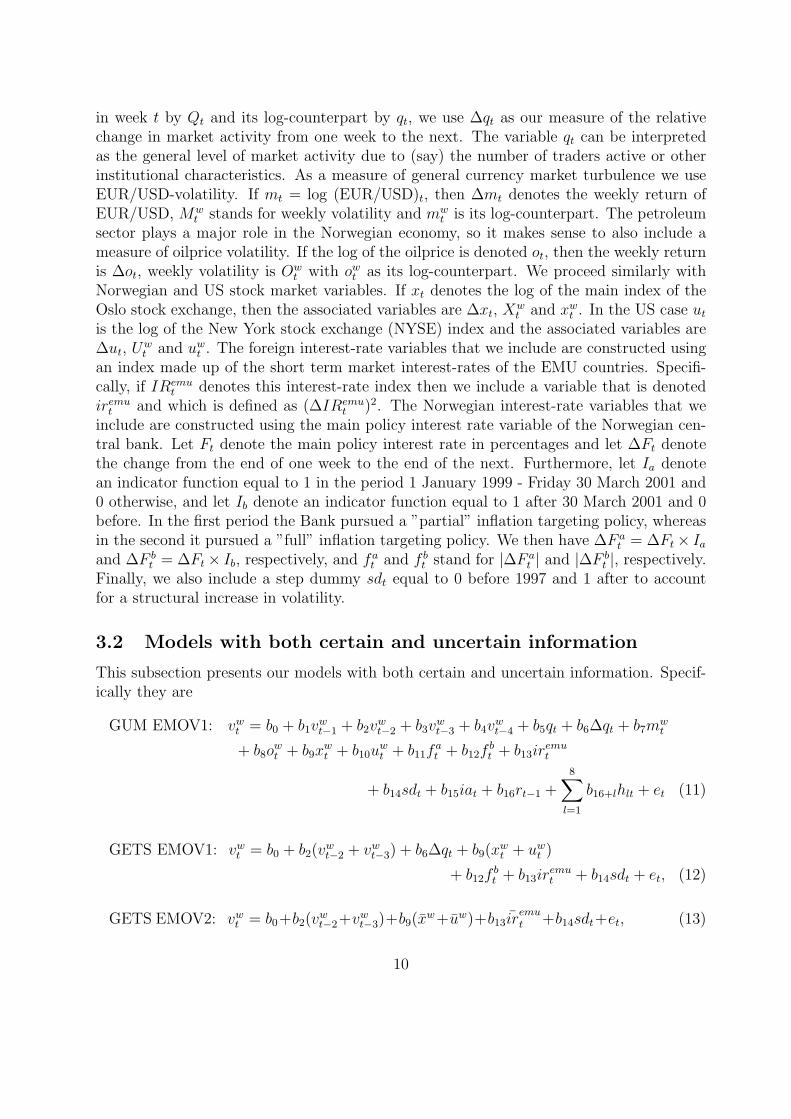
3.2 Models with both certain and uncertain information

This subsection presents our models with both certain and uncertain information. Specif-ically they are

GUM EMOV1: vwt = b0 + b1v

wt−1 + b2v

wt−2 + b3v

wt−3 + b4v

wt−4 + b5qt + b6∆qt + b7m

wt

+ b8owt + b9x

wt + b10u

wt + b11f

at + b12f

bt + b13ir

emut

+ b14sdt + b15iat + b16rt−1 +8∑

l=1

b16+lhlt + et (11)

GETS EMOV1: vwt = b0 + b2(v

wt−2 + vw

t−3) + b6∆qt + b9(xwt + uw

t )

+ b12fbt + b13ir

emut + b14sdt + et, (12)

GETS EMOV2: vwt = b0+b2(v

wt−2+vw

t−3)+b9(xw+uw)+b13ir

emut +b14sdt+et, (13)

10

GETS EMOV3: vwt = b0+b2(v

wt−2+vw

t−3)+b9(xw+uw)+b13ir

emu

t +b14sdt+et, (14)

where {et} is a sequence of innovation errors. The first specification GUM EMOV1 is ageneral and unrestricted model with both known and unknown information, whereas thesecond which is labelled GETS EMOV1 is the GETS derived counterpart. Of these two onlythe second will be used in our out-of-sample study. The second specification is obtainedby setting the first as the general unrestricted specification, and then testing restrictionsregarding the parameters with Wald-tests before the final specification is tested against theGUM. It should be noted that we only perform a single specification search where, at eachstep, we remove the regressor with highest p-value. Hoover and Perez (1999) have pointedout that performing only a single simplification search might result in ”path dependence”,in the sense that a relevant variable being removed early on in the search whereas irrelevantvariables that proxy its role are retained. However, the software PcGets version 1.0 (seeHendry and Krolzig 2001), which automates GETS multiple-path simplification search,produces a specification almost identical to (12), the only difference being that vw

t−2 isnot retained. So path-dependence does not appear to be a problem in our case. This isconsistent with White’s (1990) theorem, which implies that the path dependence problemreduces as the size of the sample increases.10 In the generation of GETS EMOV1 forecaststwo steps ahead and onwards we use forecasted values of vw

t and observed values of theother covariates. In other words, the forecasts of GETS EMOV1 are generated as if theunknown conditioning information is known. As such the accuracy of GETS EMOV1constitutes an indication of its potential for scenario analysis (policy analysis, conditionalforecasting, counterfactual analysis, etc.), since its accuracy will reflect its potential ofyielding accurate forecasts under the assumption that the unknown information is correct.The third and fourth specifications serve as a contrast to this hypothetical situation and tryto mimic more realistic circumstances by using the parameter estimates of GETS EMOV1,and by using simple forecasting rules for the uncertain information. In GETS EMOV2the variables ∆qt and f b

t are set equal to zero, and xwt , uw

t and iremut are set equal to their

sample averages xw, uw and iremut over the period 1 January 1999 - 26 December 2003.11 In

other words, variables that would have to be forecasted in a realistic setting are either setto zero or to their presumed, future sample averages. GETS EMOV3 proceeds similarlywith a single difference. Instead of averages the medians of xw

t , uwt and iremu

t , denoted xw,uw and ir

emu

t , are used.Estimation results and recursive parameter stability analysis of the first two specifica-

tions are contained in table 1, and in figures 2 and 3. Both GUM EMOV1 and GETSEMOV1 exhibit innovation errors in the sense that the nulls of no serial correlation, noautoregressive conditional heteroscedasticity and no heteroscedasticity are not rejected atthe 10% significance level, and the recursive parameter stability analysis suggests param-eters are relatively stable. For both GUM EMOV1 and GETS EMOV1 the Chow forecast

10Our sample of 573 observations is considerably larger than those investigated by Lovell (1983), Hooverand Perez (1999) and Hendry and Krolzig (1999), the sequence of studies that resulted in PcGets. WhereasLovell (1983) used only 23 observations, the other two studies employed a maximum of 140 observations.

11This sample was chosen because the volatility of rt looks relatively stable over this period.

11

and breakpoint tests do not signify at the 1% level, but the 1-step forecast tests on theother hand show some signs of instability.12 The number of spikes that exceeds the 1%critical value in the break-point tests is 11 and 13, respectively. This suggests the presenceof some structural instability since on average we would expect only 5 spikes to exceed the1% critical value (1% of 473 is just below 5). 13

3.3 Models with certain information

This subsection contains our specifications with known or relatively certain information.Specifically they are

GUM EMOV4: vwt = b0 + b1v

wt−1 + b2v

wt−2 + b3v

wt−3 + b4v

wt−4 + b14sdt

+ b16rt−1 +8∑

l=1

b16+lhlt + et, (15)

GETS EMOV4: vwt = b0 + b2(v

wt−2 + vw

t−3) + b14sdt + b18h2t + et, (16)

Realised EMOV5: vwt = b0 + b1v

rt−1 + b14sdt + b18h2t + et, (17)

Range EMOV6: vwt = b0 + b1v

hlt−1 + b14sdt + b18h2t + et, (18)

GARCH(1,1)+: rt = b0 + b1rt−1 + et, et = σtzt,

σ2t = ω + αe2

t−1 + βσ2t−1 + γ1h2t, (19)

EGARCH(1,1)+: rt = b0 + b1rt−1 + et, et = σtzt,

log σ2t = ω + α| et−1

σt−1

|+ β log σ2t−1 + γ0

et−1

σt−1

+ γ1h2t, (20)

where σt is the conditional standard deviation of rt, and {zt} is a sequence of randomvariables each with mean equal to zero conditional on the information set in question, andeach with variance equal to one conditional on the same information set. The first specifi-cation GUM EMOV4 is a general formulation nested within GUM EMOV1 but containingonly ”certain” conditioning information, that is, past and relatively certain contemporane-ous information (holiday variables). The second specification GETS EMOV4 is obtained

12If t denotes the sample size, k the number of parameters in b and M the observation at which recursiveestimation starts, then for t = M, . . . , T the 1-step, breakpoint and forecast tests are computed in PcGiveas F (1, t− k − 1), F (T − t + 1, t− k − 1) and F (t−M + 1,M − k − 1), respectively.

13The number 473 is due to the fact that the recursive estimation was initialised at observation number100.

12

through GETS-analysis of GUM EMOV4. The third specification Realised EMOV5 usesa low frequency version of lagged realised weekly volatility vr

t−1 as predictor together withthe structural step dummy sdt and the Good Friday holiday variable h2t, whereas RangeEMOV6 is identical to Realised EMOV5 except that it replaces lagged weekly realisedvolatility with lagged weekly range volatility. In the fifth and sixth specifications a con-stant b0, lagged return rt−1 and h2t are added to ”plain” GARCH(1,1) and EGARCH(1,1)specifications. In addition to the fact that the conditional variance σ2

t is modelled exponen-tially, the EGARCH differs from the GARCH by the inclusion of an asymmetry term et−1

σt−1

in the conditional variance specification. A value of γ0 unequal to zero implies asymmetryand γ0 < 0 in particular implies leverage, that is, that returns are negatively correlated withlast period’s volatility. The higher |β| the higher persistence, and a necessary condition forcovariance stationarity is |β| < 1, see Nelson (1991).

The estimation results of the six specifications are contained in tables 2, 3 and 4,and recursive parameter stability analysis of GUM EMOV4 and GETS EMOV4 in fig-ures 4 and 5. The first four specifications all exhibit innovation errors in the sense thatthe nulls of no serial correlation, no autoregressive conditional heteroscedasticity and noheteroscedasticity are not rejected at conventional significance levels, and the recursiveparameter stability analysis for GUM EMOV4 and GETS EMOV4 are similar to thoseof GUM EMOV1 and GETS EMOV1 above. Both GARCH(1,1)+ and EGARCH(1,1)+exhibit uncorrelated standardised residuals and squared standardised residuals accordingto the diagnostic tests, and the lagged return rt−1 in the mean equation is negative ascommonly found for exchange rates, but not significant. The estimates of α + β (0.129+ 0.877 = 1.006) and β (0.983) are very close to 1. This is usually interpreted as anindication of a strong persistence of shocks on the conditional variance, but in this case itis due to the structural break around the beginning of 1997, see figure 1. Finally, the valueof γ0 is insignificantly different from zero which suggests that the symmetry imposed bythe GARCH model is not restrictive.

3.4 Simple models

Our benchmark or simple models are all ARCH-specifications, and specifically they are

Historical: rt = et = σtzt, σ2t = ω (21)

RiskMetrics: rt = et = σtzt, σ2t = 0.06e2

t−1 + 0.94σ2t−1 (22)

EWMA: rt = et = σtzt, σ2t = αe2

t−1 + βσ2t−1 (23)

GARCH(1,1): rt = et = σtzt, σ2t = ω + αe2

t−1 + βσ2t−1 (24)

EGARCH(1,1): rt = et = σtzt, log σ2t = ω + α| et−1

σt−1|+ β log σ2

t−1 + γ et−1

σt−1, (25)

13

where {zt} is characterised as above. The first specification labelled Historical is a GARCH(0,0)estimated on the sample 1/1/1999 - 26/12/2003 (261 observations). In other words, it is theARCH-counterpart of the sample variance since it models volatility as non-varying, and thesample was chosen because volatility appears relatively stable graphically over this period.Failure to beat the historical variance is detrimental to models of the ARCH-class, sincethis essentially undermines their raison d’etre. The second specification is an exponen-tially weighted moving average (EWMA) with parameter values suggested by RiskMetrics(Hull 2000, p. 372).14 RiskMetrics proposed these values after having compared a rangeof combinations on various financial time series. The third specification is an EWMA withestimated parameters whereas the fourth specification is a plain GARCH(1,1) which neststhe EWMAs within it, since they can be obtained through parameter restrictions. Thefifth and final specification is a plain EGARCH(1,1).

Estimates and residual diagnostics of the simple models are contained in tables 5 and6. The estimate of the Historical specification yield standardised residuals that are un-correlated according to the AR1−10 test. Although this is not the case for the AR1−1 testwhich is not reported, the failure of the AR1−10 test to reject the null nevertheless suggeststhat the historical variance might be difficult to beat out-of-sample. In the RiskMetricsspecification the diagnostic tests suggest the values of α and β are suboptimal, since boththe standardised residuals and the squared standardised residuals are serially correlated.Indeed, the diagnostic tests of the EWMA supports this picture since there the nulls ofuncorrelated and homoscedastic standardised residuals are not rejected. The α, β esti-mates and diagnostics of the plain GARCH(1,1) specification are almost identical, and theestimate of ω is almost zero. In other words, the two specifications will produce almostidentical forecasts. In the EGARCH(1,1) model residuals are also uncorrelated whereasthe estimate of the volatility persistence parameter β is high and almost 1 (it is equal to0.981). The asymmetry parameter γ is not significant at conventional significance levels,thus suggesting the symmetry of the GARCH(1,1) is not so restrictive. Finally, comparedwith the estimates of ω, α and β in (19) and (20) they are virtually identical here. In otherwords, adding a mean specification and h2t does not seem to affect the estimates of thevariance equation noteworthy.

4 Out-of-sample forecast evaluation

This section proceeds in three steps. The first subsection contains our out-of-sample fore-cast accuracy comparison, whereas the second contains socalled Mincer-Zarnowitz (1969)regressions of observed volatility on a constant and forecasts. The third and final subsectionsheds additional light on the results by examining some of the 1-step forecast trajectories

14To be more precise, the parameter values are those suggested by the 1995 version of RiskMetrics, whichthen was part of the merchant bank J.P. Morgan. RiskMetrics is now an independent company and two ver-sions of RiskMetrics have superseded the 1995 May edition, see http://www.riskmetrics.com/techdoc.html.Note also that the parameter values are obtained with a definition of volatility that differs slightly fromthe one employed here.

14

more closely.

4.1 Out-of-sample forecast accuracy comparison

Consider a sequence of volatilities {Vk} over the forecast periods k = 1, . . . , K and acorresponding sequence of forecasts {Vk}. Our out-of-sample forecast accuracy measuresconsist of the mean absolute error (MAE) and the mean squared error (MSE), and aredefined as

MAE =1

K

K∑

k=1

|Vk − Vk|, (26)

MSE =1

K

K∑

k=1

(Vk − Vk)2, (27)

respectively.15 Both measures are symmetric in that they treat positive and negative errorsalike, and their only difference is that the latter punishes large errors more severely than theformer.16 Error-based measures are ”pure” precision measures in the sense that evaluationis based solely on the discrepancy between the forecast and the actual value. One canmake a case for the view that precision-based measures are the most appropriate whenevaluating the forecast properties of a certain modelling strategy, since this leaves openwhat the ultimate use of the model is. On the other hand, this is also a weakness sinceconsiderations pertaining to the final use of the model do not enter the evaluation.17

The values of the MAE and MSE forecast statistics are contained in tables 7 and 8.In the forecasting literature models with economic covariates are typically championedas producers of accurate long-term forecasts, but not necessarily of short-term forecastsbetter than those of ”naıve” or simple models without economic covariates. Our resultsseem to contradict this for the short term. On short horizons up to six weeks ahead GETSEMOV1, the specification with actual values on the economic variables of the right handside, performs well according to both the MAE and MSE statistics. According to the MAE

15Patton (2005) has recently argued in favour of the MSE and against the MAE in volatility forecastcomparison. It should be noted however that his argument applies (under certain assumptions) when theproblem to be solved is to choose an σ2

t such that expected L(σ2t , σ2

t ) is minimised, where L(·) is a lossfunction. In explanatory modelling on the other hand, as we argued in subsection 2.1, the problem tobe solved is to choose an σ2

t such that expected L(r2t , σ2

t ) is minimised. This is a qualitatively importantdifference and it is not clear that Patton’s conclusions hold when the problem is formulated in this way.

16An alternative to the MAE and MSE are their relative counterparts which scale the error Vk − Vk

by either Vk or Vk. The disadvantage with the relative counterparts is that they may favour or disfavourmodels that either systematically overpredicts or underpredicts, regardless of how well they fare accordingto the MAE and MSE criteria.

17Several other approaches to out-of-sample forecast comparison have been proposed. One consists ofadding other ingredients to the evaluation scheme, see for example West et al. (1993) where the expectedutility of a risk averse investor serves as the ranking criterion. Similarly, Engle et al. (1993) providea methodology in which the profitability of a certain trading strategy ranks the forecasts. Yet anotherapproach takes densities as the object of interest, see Diebold et al. (1998), whereas Lopez (2001) hasproposed a framework that provides probability forecasts of the event of interest.

15

it comes 1st, 2nd, 3rd and 3rd up to six weeks ahead, whereas according to the MSE itcomes 1st on the same forecast horizons. On longer horizons, however, results are moremixed. For 12 and 18 weeks ahead the GETS EMOV1 comes 10th and 12th (last) accordingto the MAE, and 9th for both the 12 and 18 horizons according to the MSE. One mightsuggest that this is due to structural instability, but the results of the other GETS modelsindicate it is not that straightforward. Indeed, generally the GETS models (EMOV1-4)do notably better according to the MSE measure than the MAE measure, which suggeststhat the usefulness of GETS modelling increases when larger errors are punished more.The most extreme case is GETS EMOV4 which 12 and 18 weeks ahead comes 12th (last)and 11th (second-to-last) according to the MAE measure, and 4th and 4th according tothe MSE measure. This suggests that the poor performance of GETS EMOV3 on longerhorizons is not due to parameter instability.

In a practical forecasting situation the actual values on the right hand side of theGETS EMOV1 specification would have to be forecasted, and GETS EMOV2 and GETSEMOV3 try to mimic such a situation. Both models are relatively consistent and performcomparatively well on shorter horizons, in particular according to the MSE measure, butas long as no statistical tests are involved it is unclear whether it is significantly superioror inferior to any particular model. On the first four horizons the GETS EMOV2 comes3rd, 5th, 5th and 6th according to the MAE, and 4th, 4th, 4th and 5th according to theMSE. On the same horizons the GETS EMOV3 comes 4th, 6th, 7th and 8th according tothe MAE, and 3rd, 3rd, 3th and 4rd according to the MSE. For 12 and 18 weeks aheadthe GETS EMOV4 and GETS EMOV5 do not fare well according to the MAE, since theycome 7th or worse. According to the MSE on the other hand they come 4th or better.

Although the MAE and MSE measures suggest that the GETS models perform rela-tively well compared with the other models, it should be stressed that so do some of thesimple models at times. For example, according to the MAE the Historical specification,that is, the constant model of volatility, comes 2nd at the 1 week horizon, 4rd at the 2and 3 weeks horizons, and according to the MSE it is distinguishable from the best model12 and 18 weeks ahead only at the third decimal. Similarly, the Range EMOV6, that is,the specification that uses lagged range volatility as predictor, comes 1st on the 2, 3 and 6week horizons according to the MAE. The RiskMetrics, GARCH and EGARCH specifica-tions do not do particularly well at short horizons, that is, on horizons in which one wouldexpect them to do well. Not once does any of the five specifications beat Historical 1 to 3weeks ahead according to both MAE and MSE.

4.2 1-step Mincer-Zarnowitz regressions

A simple statistical way of evaluating forecast models is by regressing the variable to beforecasted on a constant and on the forecasts, socalled Minzer-Zarnowitz (1969) regressions,see Andersen and Bollerslev (1998) and Patton (2005) for a discussion of their use in

16

volatility forecast evaluation.18 In our case this proceeds by estimating the specification

r2t = a + bVt + et, (28)

where r2t is observed volatility, Vt is the 1-step forecast and et is the error term. Ideally,

a should equal zero and b should equal one—since these constitute conditions for ”un-biasedness”, and the fit should be high. Table 9 contains the regression output.19 Onespecification stands out according to the majority of the criteria, namely GETS EMOV1.Its estimate of a is not significantly different from zero, the estimate of b is positive andsignificantly different from zero, the joint restriction a = 0, b = 1 is not rejected at con-ventional significance levels, and its R2 is 0.26. This is substantially higher than any ofthe R2s cited in Andersen and Bollerslev (1998, pp. 890-891) (the typical R2 they cite isaround 0.03 and the highest is 0.11), and must be very close to—if not exceeding—theirpopulation upper bound of R2:

”..with conditional Gaussian errors the R2(m) from a correctly specified GARCH(1,1)

model is bounded from above by 13, while with conditional fat-tailed errors the

upper bound is even lower. Moreover, with realistic parameter values for α(m)

and β(m), the population value for the R2(m) statistic is significantly below this

upper bound”—Andersen and Bollerslev (1998, p. 892).

In other words, although the unusually high R2 of GETS EMOV3 might be due tosample specificity, it nevertheless suggests the poor forecasting performance of r2

t byARCH-models can be improved upon substantially. Moreover, apart from the RiskMet-rics specification Historical beats the other five members of the ARCH-family (EWMA,GARCH(1,1), EGARCH(1,1), GARCH(1,1)+ and EGARCH(1,1)+), and the four modelsGETS EMOV1-4 perform better than Historical according to R2. Also, in none of thesefour specifications is neither a significantly different from zero, nor is the joint restrictiona = 0, b = 1 rejected. Apart from Historical and RiskMetrics, the restriction a = 0, b = 1is rejected at the 5% level in all the ARCH-specifications, and a is significantly differentfrom zero.

4.3 Explaining the forecast results

An important part of an out-of-sample study consists of explaining the results, and to thisend figure 6 provides a large part of the answer. The figure contains the out-of-sampletrajectories of squared NOK/EUR log-returns in percent r2

t , the 1-step forecasts of GETSEMOV1 and the 1-step forecasts of Historical, and the figure provides some interesting

18It should be stressed though that their discussion concerns forecasting the latent volatility rather thanobserved volatility, as is the case in this study.

19Patton (2005, footnote on p. 6) has noted that the residuals in Mincer-Zarnowitz regressions typicallyare serially correlated and that this should be taken into account by using (say) Newey and West (1987)standard errors. In our case the residuals are not serially correlated according to standard tests, butadmittedly it might be undetectable due to our relatively small sample.

17

insights on the forecast accuracy results. First, the series of r2t seems to be characterised

by some occasional large values but little volatility persistence in the sense that large valuesdo not tend to follow each other. Indeed, only at two instances is a large value followedby another, and for a relatively large portion of the sample r2

t stays rather low. Thisexplains to some extent the forecast accuracy of Historical. It also explains to some extentthe success of Range EMOV6, since its trajectory—which is not contained in the figure—isvery similar to Historical’s. Second, in the 5th and in the 11th weeks of the forecast sampleNorges Bank changed its main policy interest rate. This is reflected in the large valuesof r2

t in the 5th and 11th weeks, and explains the forecast accuracy of GETS EMOV1 (itcontains policy interest rate changes as a predictor) and its unusually high R-squared inthe 1-step forecast regressions. Finally, the other explanatory variables included in GETSEMOV1 are probably the reason why it also follows r2

t relatively well at other instanceswhen r2

t moves substantially. But it should be noted that the explanatory regressors inGETS EMOV1 also seem to induce notable forecast error on at least two occasions. Inother words, although the forecast success of GETS EMOV1 is due to the explanatoryvariables, there are also signs that they may have the opposite effect, namely increasingthe forecast error. All in all, then, the forecast results suggest the GETS EMOV1 is usefulfor conditional forecasting but that it does not improve upon the forecasting by simplemodels when the explanatory variables are unchanging or move little.

5 Conclusions

This study has evaluated the out-of-sample forecast accuracy of GETS derived models ofweekly NOK/EUR volatility. The GETS specification that uses actual values of uncertaininformation is found to perform particularly well when it is able to explain big movements inthe exchange rate, but not necessarily better than simple models like the constant volatilitymodel when the exchange rate does not move much or when it is unable to explain themovement. Models of the GARCH(1,1) and EGARCH(1,1) types do not fare particularlywell and the reason is that large values (in the absolute sense) of returns do not seem tocome in pairs nor in longer sequences at the weekly frequency. Rather, big movements inthe exchange rate seems more to be a ”one off” phenomenon.

Overall, then, our results suggest GETS derived models of observable volatility are notinferior to the comparison models, and that they are particularly useful in conditional fore-casting. This suggests several lines for further research. First, the generality of our resultsmust be established. Is GETS-modelling of financial volatility useful on higher frequenciesthan the weekly? On other financial assets? Second, contrary to McAleer’s (2005) asser-tion, automated GETS-modelling of financial volatility can be readily implemented andshould be investigated more fully.

18

References

Andersen, T. G. and T. Bollerslev (1998). Answering the skeptics: Yes, standard volatilitymodels do provide accurate forecasts. International Economic Review 39, 885–905.

Andersen, T. G., T. Bollerslev, and S. Lange (1999). Forecasting Financial Market Volatil-ity: Sample Frequency vis-a-vis Forecast Horizon. Journal of Empirical Finance 6,457–477.

Bauwens, L., D. Rime, and G. Sucarrat (2006). Exchange Rate Volatility and the Mixtureof Distribution Hypothesis. Empirical Economics 30, 889–911.

Bollerslev, T. (1986). Generalized autoregressive conditional heteroscedasticity. Journal ofEconometrics 31, 307–327.

Bollerslev, T. and J. Wooldridge (1992). Quasi-Maximum Likelihood Estimation and In-ference in Dynamic Models with Time Varying Covariances. Econometric Reviews 11,143–172.

Campos, J., N. R. Ericsson, and D. F. Hendry (2005). General-to-Specific Modeling: AnOverview and Selected Bibliography. In J. Campos, D. F. Hendry, and N. R. Ericsson(Eds.), General-to-Specific Modeling. Cheltenham: Edward Elgar Publishing.

Diebold, F., T. Gunther, and A. Tay (1998). Evaluating Density Forecasts with Applica-tions to Financial Risk Management. International Economic Review 39, 863–883.

Engle, R., C.-H. Hong, A. Kane, and J. Noh (1993). Arbitrage Valuation of VarianceForecasts with Simulated Options. In D. Chance and R. Trippi (Eds.), Advances inFutures and Options Research. Greenwich, Connecticut: JAI Press.

Geweke, J. (1986). Modelling the Persistence of Conditional Variance: A Comment. Econo-metric Reviews 5, 57–61.

Gilbert, C. L. (1989). Lse and the british approach to time series econometrics. OxfordEconomic Papers 41, 108–128.

Gilbert, C. L. (1990). Professor Hendry’s Econometric Methodology. In C. W. Granger(Ed.), Modelling Economic Series. Oxford: Oxford University Press. Earlier publised inOxford Bulletin of Economics and Statistics 48 (1986), pp. 283-307.

Hendry, D. F. (1987). Econometric Methodology: A Personal Perspective. In T. F. Bewley(Ed.), Fifth World Congress of the Econometric Society. Oxford: Oxford UniversityPress.

Hendry, D. F. (1995). Dynamic Econometrics. Oxford: Oxford University Press.

Hendry, D. F. (1997). On Congruent Econometric Relations: A Comment. Carnegie-Rochester Conference Series on Public Policy 47, 163–190.

19

Hendry, D. F. (2003). J. Denis Sargan and the Origins of LSE Econometric Methodology.Econometric Theory 19, 457–480.

Hendry, D. F. and H.-M. Krolzig (1999). Improving on ’Data Mining Reconsidered’ byK.D. Hoover and S.J. Perez. Econometrics Journal 2, 202–219.

Hendry, D. F. and H.-M. Krolzig (2001). Automatic Econometric Model Selection usingPcGets. London: Timberlake Consultants Press.

Hendry, D. F. and H.-M. Krolzig (2004). We Ran One Regression. Research in Progress.Http://www.nuff.ox.ac.uk/Economics/Papers/2004/w17/OneReg.pdf.

Hendry, D. F. and J.-F. Richard (1990). On the Formulation of Empirical Models inDynamic Econometrics. In C. W. Granger (Ed.), Modelling Economic Series. Oxford:Oxford University Press. Earlier in Journal of Econometrics 20 (1982), pp. 3-33.

Hoover, K. D. and S. J. Perez (1999). Data Mining Reconsidered: Encompassing and theGeneral-to-Specific Approach to Specification Search. Econometrics Journal 2, 167–191.

Hull, J. C. (2000). Options, Futures and Other Derivatives. London: Prentice Hall Inter-national. Fourth Edition.

Jansen, E. (2002). Statistical Issues in Macroeconomic Modelling. Scandinavian Journalof Statistics 29, pp. 193–217.

Jarque, C. and A. Bera (1980). Efficient Tests for Normality, Homoskedasticity, and SerialIndependence of Regression Residuals. Economics Letters 6, 255–259.

Jorion, P. (1995). Predicting Volatility in the Foreign Exchange Markets. The Journal ofFinance 50, 507–528.

Ljung, G. and G. Box (1979). On a Measure of Lack of Fit in Time Series Models.Biometrika 66, 265–270.

Lopez, J. A. (2001). Evaluating the Predictive Accuracy of Volatility Models. Journal ofForecasting 20, 87–109.

Lovell, M. C. (1983). Data Mining. The Review of Economics and Statistics 65, 1–12.

McAleer, M. (2005). Automated inference and learning in modeling financial volatility.Econometric Theory 21, 232–261.

Mincer, J. and V. Zarnowitz (1969). The Evaluation of Economic Forecasts. In J. Zarnowitz(Ed.), Economic Forecasts and Expectations. New York: National Bureau of EconomicResearch.

20

Mizon, G. (1995). Progressive Modeling of Macroeconomic Time Series: The LSEMethodology. In K. D. Hoover (Ed.), Macroeconometrics. Developments, Tensions andProspects. Kluwer Academic Publishers.

Nelson, D. B. (1991). Conditional Heteroscedasticity in Asset Returns: A New Approach.Econometrica 51, 485–505.

Newey, W. and K. West (1987). A Simple Positive Semi-Definite, Heteroskedasticity andAutocorrelation Consistent Covariance Matrix. Econometrica 55, 703–708.

Pantula, S. (1986). Modelling the Persistence of Conditional Variance: A Comment.Econometric Reviews 5, 71–73.

Patton, A. J. (2005). Volatility Forecast Evaluation and Comparison Using ImperfectVolatility Proxies. Downloadable from http://fmg.lse.ac.uk/˜patton/research.html.

West, K., H. Edison, and D. Cho (1993). A Utility Based Comparison of Some Models forExchange Rate Volatility. Journal of International Economics 35, 23–45.

White, H. (1980). A Heteroskedasticity-Consistent Covariance Matrix and a Direct Testfor Heteroskedasticity. Econometrica 48, 817–838.

White, H. (1990). A consistent model selection procedure based on emphm-testing. InC. W. Granger (Ed.), Modelling Economic Series: Readings in Econometric Methodol-ogy. Oxford: Clarendo Press.

21

Appendix: Data transformations and sources

The data transformations were undertaken in Ox 3.4 and EViews 5.1.

St BID NOK/1EUR closing value of the last trading day of week t. Before 1.1.1999the BID NOK/1EUR rate is obtained by the formula BID NOK/100DEM ×0.0195583, where 0.0195583 is the official DEM/1EUR conversion rate 1.95583DEM = 1 EUR divided by 100. The source of the BID NOK/100DEM seriesis Olsen Financial Technologies and the source of the BID NOK/1EUR seriesis Reuters.

rt (log St − log St−1)× 100

V wt {{log[St + I(St = St−1) × 0.0009] − log(St−1)} × 100}2. I(St = St−1) is an

indicator function equal to 1 if St = St−1 and 0 otherwise, and St = St−1

occurs for t = 10/6/1994, t = 19/8/1994 and t = 17/2/2000.

vwt log V w

t

V rt

∑n[log(Sn/Sn−1)×100]2, where n = 1(t), 2(t), ..., N(t) and 1(t)−1 = N(t−1).

S1(t) is the first BID NOK/1EUR opening exchange rate of week t, S2(t) isthe first closing rate, S3(t) is the second opening rate, and so on, with SN(t)

denoting the last closing rate of week t, that is, SN(t) = St.

vrt log V r

t

V hlt [log(Sh

t /Slt)× 100]2, where Sh

t and Slt are the maximum and minimum values

of bid NOK/EUR in week t.

vhlt log V hl

t

Mt BID USD/EUR closing value of the last trading day of week t. Before1.1.1999 the BID USD/EUR rate is obtained with the formula 1.95583/(BIDDEM/USD). The source of the BID DEM/USD and BID USD/EUR series isReuters.

mt log Mt

Mwt {{log[Mt + I(Mt = Mt−1)× 0.0009]− log(Mt−1)}× 100}2. I(Mt = Mt−1) is an

indicator function equal to 1 if Mt = Mt−1 and 0 otherwise.

mwt log Mw

t

Qt Weekly number of NOK/EUR quotes (NOK/100DEM before 1.1.1999). Theunderlying data is a daily series from Olsen Financial Technologies, and theweekly values are obtained by summing the values of the week.

qt log Qt. This series is ”synthetic” in that it has been adjusted for changes inthe underlying quote collection methodology at Olsen Financial Technologies.More precisely qt has been generated under the assumption that ∆qt is equalto zero in the weeks containing Friday 17 August 2001 and Friday 5 September2003, respectively. In the first week the underlying feed was changed fromReuters to Tenfore, and on the second a feed from Oanda was added.

22

∆qt qt− qt−1. The values of this series has been set to zero in the weeks containingFriday 24 August 2001 and Friday 5 September 2003, respectively.

Ot Closing value of the Brent Blend spot oilprice in USD per barrel in the lasttrading day of week t. The untransformed series is Bank of Norway databaseseries D2001712.

ot log Ot

Owt {{log[Ot + I(Ot = Ot−1) × 0.009] − log(Ot−1)} × 100}2. I(Ot = Ot−1) is an

indicator function equal to 1 if Ot = Ot−1 and 0 otherwise, and Ot = Ot−1

occurs three times, for t = 1/7/1994, t = 13/10/1995 and t = 25/7/1997.

owt log Ow

t

Xt Closing value of the main index of the Norwegian Stock Exchange (TOTX) inthe last trading day of week t. The source of the daily untransformed series isEcoWin series ew:nor15565.

xt log Xt

Xwt {[log(Xt/Xt−1)]× 100}2. Xt = Xt−1 does not occur for this series.

xwt log Xw

t

Ut Closing value of the composite index of the New York Stock Exchange (theNYSE index) in the last trading day of week t. The source of the daily un-transformed series is EcoWin series ew:usa15540.

Uwt {[log(Ut/Ut−1)]× 100}2. Ut = Ut−1 does not occur for this series.

uwt log Uw

t

IRemut Average of closing values of the 3-month market interest rates of the European

Monetary Union (EMU) countries in the last trading day of week t. The sourceof the daily untransformed series is EcoWin series ew:emu36103.

iremut (∆IRemu

t )2.

Ft The Norwegian central bank’s main policy interest-rate, the socalled ”folio”,at the end of the last trading day of week t. The source of the untransformeddaily series is Norges Bank’s webpages.

fat |∆Ft|× Ia, where Ia is an indicator function equal to 1 in the period 1 January

1999 - Friday 30 March 2001 and 0 elsewhere

f bt |∆Ft| × Ib, where Ib is an indicator function equal to 1 after Friday 30 March

2001 and 0 beforeidt Russian moratorium impulse dummy, equal to 1 in the week containing Friday

28 August 1998 and 0 elsewhere.

sdt Step dummy, equal to 0 before 1997 and 1 thereafter.

iat Skewness term, equal to 1 when rt > 0 and 0 otherwise.

23

hlt l = 1, 2, . . . , 8. Holiday variables with values equal to the number of officialNorwegian holidays that fall on weekdays. For example, if 1 January falls on aSaturday then h1t is equal to 0, whereas if 1 January falls on a Monday, thenh1t is equal to 1. h2t is associated with Maundy Thursday and Good Fridayand thus always equal to 2, h3t with Easter Monday and thus always equalto 1, h4t with Labour Day (1 May), h5t with the Norwegian national day (17May), h6t with Ascension Day, h7t with Whit Monday and h8t with Christmas(Christmas Day and Boxing Day). Source: Http://www.timeanddate.com.

24

Table 1: GUM and GETS regressions of log ofweekly NOK/EUR volatility on both certainand uncertain informationParameter (11) (12)

Est. Pval. Est. Pval.b0 -3.304 0.03 -3.035 0.00b1 0.013 0.76b2 0.070 0.07 0.079 0.00b3 0.093 0.03b4 -0.001 0.99b5 0.063 0.76b6 1.024 0.00 1.066 0.00b7 0.067 0.13b8 0.021 0.65b9 0.125 0.01 0.119 0.00b10 0.113 0.01b11 -0.256 0.83b12 3.775 0.00 3.751 0.00b13 4.797 0.02 4.819 0.00b14 1.130 0.00 1.238 0.00b15 -0.127 0.52b16 -0.025 0.85b17 -1.207 0.16b18 -0.141 0.62b19 0.330 0.64b20 -0.710 0.22b21 0.195 0.71b22 0.653 0.25b23 0.019 0.98b24 -0.036 0.96

R2 0.21 0.20AR1−10 5.11 0.88 3.07 0.98ARCH1−10 7.00 0.73 8.71 0.56Het. 39.72 0.44 11.46 0.41Hetero. 179.98 0.92 14.60 0.95Obs. 568 569

Note: See table 2.

25

Table 2: GUM and GETS Regressions of logof weekly NOK/EUR volatility on certain in-formation only

Parameter (15) (16)Est. Pval. Est. Pval.

b0 -2.918 0.00 -2.946 0.00b1 0.030 0.48b2 0.077 0.04 0.088 0.00b3 0.093 0.03b4 -0.020 0.64b13 1.448 0.00 1.428 0.00b14 -0.009 0.96b16 -0.024 0.86b17 -0.820 0.30b18 -0.500 0.07 -0.478 0.08b19 0.435 0.59b20 -0.751 0.17b21 0.170 0.72b22 0.346 0.55b23 -0.446 0.56b24 -0.625 0.37


Note: Computations are in EViews 5.1 with OLSestimation. All specifications use heteroscedastic-ity consistent standard errors of the White (1980)type, Pval stands for p-value and corresponds to atwo-sided test with zero as null, AR1−10 is the χ2

version of the Lagrange-multiplier test for seriallycorrelated residuals up to lag 10, ARCH1−10 isthe χ2 version of the Lagrange-multiplier testfor serially correlated squared residuals up to lag10, and Het. and Hetero. are the χ2 versions ofWhite’s (1980) heteroscedasticity tests withoutand with cross products, respectively.

26

Table 3: Regressions of log of weekly volatilityon log of lagged realised volatility and on logof lagged range volatility


b0 -2.774 0.00 -3.018 0.00b1 0.304 0.00 0.348 0.00b14 1.158 0.00 1.057 0.00b18 -0.510 0.07 -0.527 0.06


Note: See table 2.

27

Table 4: ARCH models of rt with certain infor-mation.Parameter (19) (20)

Est. Pval. Est. Pval.b0 -0.017 0.42 -0.007 0.77b1 -0.055 0.33 -0.067 0.21

ω 0.009 0.07 -0.209 0.00α 0.129 0.01 0.285 0.00β 0.877 0.00 0.983 0.00γ0 0.012 0.86γ1 -0.043 0.08 -0.171 0.35

LogL. -658.74 -571.98AR1−10 9.64 0.47 14.62 0.15ARCH1−10 4.80 0.90 5.75 0.84JB 664.93 0.00 417.11 0.00Obs. 571 571

Note: Computations are in EViews 5.1 withrobust standard errors of the Bollerslev andWooldridge (1992) type. Pval stands for p-valueand corresponds to a two-sided test with zeroas null, LogL stands for log-likelihood, AR1−10

is the Ljung and Box (1979) test for serial cor-relation in the standardised residuals up to lag10, ARCH1−10 is the Ljung and Box (1979) testfor serial correlation in the squared standardisedresiduals up to lag 10, and JB is the Jarqueand Bera (1980) test for non-normality in thestandardised residuals.

28

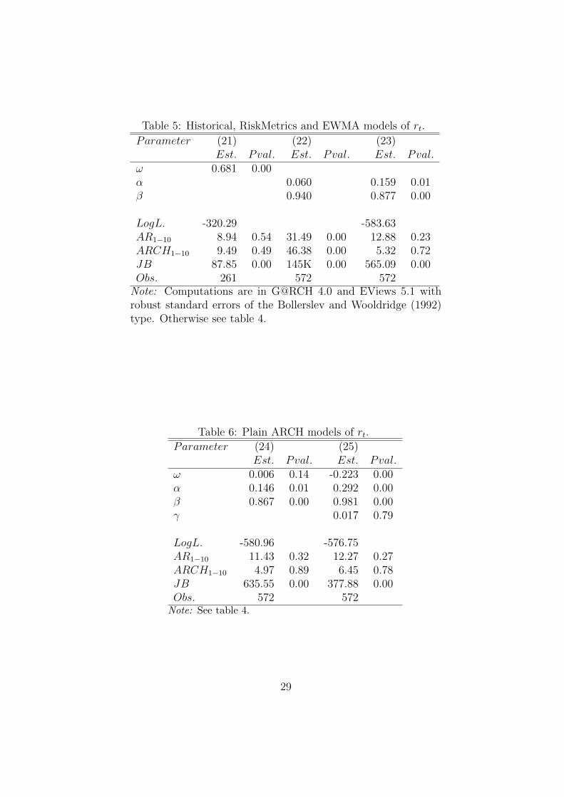
Table 5: Historical, RiskMetrics and EWMA models of rt.

Parameter (21) (22) (23)Est. Pval. Est. Pval. Est. Pval.

ω 0.681 0.00α 0.060 0.159 0.01β 0.940 0.877 0.00

LogL. -320.29 -583.63AR1−10 8.94 0.54 31.49 0.00 12.88 0.23ARCH1−10 9.49 0.49 46.38 0.00 5.32 0.72JB 87.85 0.00 145K 0.00 565.09 0.00Obs. 261 572 572

Note: Computations are in G@RCH 4.0 and EViews 5.1 withrobust standard errors of the Bollerslev and Wooldridge (1992)type. Otherwise see table 4.

Table 6: Plain ARCH models of rt.


ω 0.006 0.14 -0.223 0.00α 0.146 0.01 0.292 0.00β 0.867 0.00 0.981 0.00γ 0.017 0.79

LogL. -580.96 -576.75AR1−10 11.43 0.32 12.27 0.27ARCH1−10 4.97 0.89 6.45 0.78JB 635.55 0.00 377.88 0.00Obs. 572 572

Note: See table 4.

29

Table 7: MAE forecast statistics1-step 2-step 3-step 6-step 12-step 18-step

GETS EMOV1 0.74 0.75 0.65 0.62 0.66 0.74GETS EMOV2 0.83 0.83 0.72 0.67 0.64 0.66GETS EMOV3 0.85 0.85 0.73 0.70 0.66 0.68

GETS EMOV4 0.90 0.90 0.77 0.74 0.70 0.73Realised EMOV5 0.90 0.78 0.63 0.62 0.58 0.61Range EMOV6 0.96 0.74 0.60 0.60 0.56 0.59GARCH(1,1)+ 0.98 0.91 0.72 0.65 0.56 0.62EGARCH(1,1)+ 1.02 1.96 1.48 0.85 0.55 0.65

Historical 0.81 0.82 0.70 0.69 0.65 0.67RiskMetrics 0.92 1.00 0.79 0.77 0.64 0.58EWMA 1.06 1.24 0.97 0.83 0.63 0.61GARCH(1,1) 0.99 1.16 0.89 0.78 0.61 0.61EGARCH(1,1) 1.00 0.88 0.75 0.66 0.59 0.67

Note: Bold value indicates minimum in its column.

Table 8: MSE forecast statistics1-step 2-step 3-step 6-step 12-step 18-step

GETS EMOV1 1.61 1.64 1.07 1.07 1.25 1.40GETS EMOV2 2.07 2.10 1.21 1.20 1.02 1.12GETS EMOV3 2.06 2.09 1.21 1.19 1.02 1.12

GETS EMOV4 2.04 2.06 1.22 1.19 1.03 1.12Realised EMOV5 2.14 2.23 1.24 1.25 1.06 1.17Range EMOV6 2.25 2.37 1.39 1.41 1.21 1.34GARCH(1,1)+ 2.31 2.23 1.25 1.24 1.20 1.42EGARCH(1,1)+ 2.29 4.82 2.81 1.35 1.20 1.50

Historical 2.13 2.16 1.20 1.19 1.02 1.12RiskMetrics 2.18 2.66 1.37 1.47 1.17 1.21EWMA 2.44 4.76 2.54 2.05 1.31 1.39GARCH(1,1) 2.33 4.25 2.18 1.85 1.28 1.39EGARCH(1,1) 2.29 2.19 1.48 1.43 1.33 1.56

Note: Bold value indicates minimum in its column.

30

Table 9: Mincer-Zarnowitz regressions of r2t on a

constant and 1-step out-of-sample forecasts (K =61)

a b R2 Pval.GETS EMOV1 -0.17 1.36 0.26 0.79

[0.63] [0.02]

GETS EMOV2 -0.32 1.65 0.03 0.76[0.78] [0.36]

GETS EMOV3 -0.32 1.54 0.03 0.90[0.78] [0.36]

GETS EMOV4 -0.20 1.20 0.03 0.91[0.82] [0.31]

Realised EMOV5 0.75 0.10 0.00 0.64[0.37] [0.91]

Range EMOV6 1.42 -0.66 0.01 0.00[0.03] [0.26]

GARCH(1,1)+ 0.92 -0.08 0.00 0.00[0.01] [0.80]

EGARCH(1,1)+ 0.93 -0.09 0.00 0.02[0.02] [0.83]

Historical - 1.24 0.00 0.39[0.00]

RiskMetrics 0.93 -0.10 0.00 0.13[0.08] [0.86]

EWMA 0.95 -0.10 0.00 0.00[0.01] [0.70]

GARCH(1,1) 0.96 -0.12 0.00 0.00[0.01] [0.69]

EGARCH(1,1) 0.98 -0.14 0.00 0.01[0.01] [0.71]

Note: Numbers in square brackets denote the p-valuesof a two-sided coefficient hypothesis test with zero asthe null hypothesis, and the last column denotes thep-value of a χ2(2) Wald test of the joint restrictiona = 0, b = 1. Otherwise see table 2.

31

7.2

7.6

8.0

8.4

8.8

9.2

93 94 95 96 97 98 99 00 01 02 03 04

bid NOK/EUR (21:50 gmt)

Exchange rate stabilisation Partial inflationtargeting

Full inflationtargeting

Forecastperiod

-4

-2

0

2

4

6

93 94 95 96 97 98 99 00 01 02 03 04

weekly NOK/EUR return



Forecastperiod

-12

-8

-4

0

4

93 94 95 96 97 98 99 00 01 02 03 04

log of weekly squared NOK/EUR return



Forecastperiod

Figure 1: Bid NOK/EUR at 21:50 GMT in the last trading day of the week (denoted St inthe text) in the upper graph, log-return rt in the middle graph and log of r2

t in the bottomgraph from 8 January 1993 to 25 February 2005.

32

100 150 200 250 300 350 400 450 500 550

0

1

21−step forecast Chow test 1%

100 150 200 250 300 350 400 450 500 550

0.50

0.75

1.00

Breakpoint Chow test 1%

100 150 200 250 300 350 400 450 500 550

0.25

0.50

0.75

1.00

Forecast Chow test 1%

Figure 2: Recursive analysis of GUM EMOV1. Computations are in PcGive 10.4 withOLS and initialisation at observation number 100.

33

150 300 450

−4

−3

−2 b0 × +/−2SE

150 300 450

0.0

0.1

0.2 b2 × +/−2SE

150 300 450

0

1

2

3b6 × +/−2SE

150 300 450

0.00.10.20.3 b9 × +/−2SE

150 300 450

−5

0

5

10b12 × +/−2SE

150 300 450

0.0000

0.0005

0.0010

0.0015 b13 × +/−2SE

150 300 450

0

5 b14 × +/−2SE

150 300 450

1

21−step forecast test 1%

150 300 450

0.25

0.50

0.75

1.00Breakpoint test 1%

150 300 450

0.25

0.50

0.75

1.00Forecast test 1%

Figure 3: Recursive analysis of GETS EMOV1. Computations are in PcGive 10.4 withOLS and initialisation at observation number 100.

34

100 150 200 250 300 350 400 450 500 550

0

1

2 1−step forecasting Chow test 1%

100 150 200 250 300 350 400 450 500 550

0.50

0.75

1.00Breakpoint Chow test 1%

100 150 200 250 300 350 400 450 500 550

0.25

0.50

0.75

1.00Forecast Chow test 1%

Figure 4: Recursive analysis of GUM EMOV4. Computations are in PcGive 10.4 withOLS and initialisation at observation number 100.

35

200 300 400 500

−4

−3

−2 b0 × +/−2SE

200 300 400 500

−0.1

0.0

0.1

0.2 b2 × +/−2SE

200 300 400 500

0

5 b14 × +/−2SE

200 300 400 500

−2

−1

0

1 b18 × +/−2SE

200 300 400 500

0

1

2 1−step forecast test 1%

200 300 400 500

0.25

0.50

0.75

1.00Breakpoint test 1%

200 300 400 500

0.50

0.75

1.00Forecast test 1%

Figure 5: Recursive analysis of GETS EMOV4. Computations are in PcGive 10.4 withOLS and initialisation at observation number 100.

36

0

2

4

6

8

10

2004M01 2004M04 2004M07 2004M10 2005M01

r^2 GETS EMOV 1 Historical

30.1 12.3

Figure 6: Out-of-sample trajectories of r2t , GETS EMOV1 and Historical. Vertical lines

indicate weeks in which Norges Bank changed their main policy interest rate.

37

core discussion paper 2006/21

Documents