Electronic copy available at: http://ssrn.com/abstract=1946806

Corruption in Procurement: Evidence from FinancialTransactions Data∗

Maxim Mironov and Ekaterina Zhuravskaya†

This draft: January 2014

Abstract

This paper develops a novel approach to measuring illicit payments of firms to politicians

based on objective financial data from Russia. Firms with public procurement revenue

substantially increase tunneling around regional elections, whereas neither the tunneling

activity of firms without procurement revenue, nor the legitimate financial activity of firms

exhibits a pronounced political cycle. We show that the correlation between tunneling

around elections and procurement contacts across firms is an indicator of corruption. We use

the variation in the strength of this correlation to build a locality-level measure of corruption.

Using this measure, we test and reject the “efficient grease” hypothesis by showing that in

more corrupt localities procurement contracts are allocated to less productive firms.

∗We thank Ray Ball, Francesco Caselli, Matthew Gentzkow, Sergei Guriev, Irena Gros-feld, Peter Lorentzen, Christian Leuz, Garen Markarian, Elena Paltseva, Paolo Porchia,Paola Sapienza, Andrei Shleifer, Jeremy Stein, Marco Trombetta and the participants of theNES/SITE/KEI/BEROC/BICEPS retreat in Ventspils, the ISNIE Annual Conference, NBERPolitical Economics meetings, 2014 ASSA/AEA in Philadelphia, and the seminar participants atUTDT, IE Business School, EDRD, Paris School of Economics, New Economic School, SciencesPo, and Toulouse School of Economics for helpful comments. The paper was previously circulatedunder a title: “Corruption in Procurement and Shadow Campaign Financing.”†Mironov is from IE Business School, Madrid; Zhuravskaya is from the Paris School of Eco-

nomics (EHESS) and New Economic School. Please send correspondence to: Ekaterina Zhu-ravskaya, Paris School of Economics, 48 boulevard Jourdan, 75014 Paris, France, Email: Zhu-ravsk@pse.ens.fr.

Electronic copy available at: http://ssrn.com/abstract=1946806

1 Introduction

Does corruption improve efficiency by allowing most productive firms to get around inefficient

red tape or, on the contrary, corruption gives an advantage to less productive firms with political

connections, increasing productive inefficiency? In theory, both answers are possible (see, for

instance, the survey by Aidt, 2003). The empirical research on this question, however, is rather

limited. The lack of evidence is not surprising: bribes are unobservable and corruption is very

difficult to measure. In this paper we develop a novel approach to measuring illegal payments

of firms to politicians and show that when the allocation of procurement contracts depends on

whether firms make such illegal payments, less productive firms get procurement contracts.

The last two decades saw a sharp increase in the body of research focusing on measuring

corruption. Most measures of corruption are based on perceptions, such as expert opinions or

surveys, in which individuals and firm managers are questioned about their assessment of corrup-

tion. Due to the secretive nature of corruption, in most cases, surveys do not give information

sufficient to test hypotheses about the welfare effects of corruption (for difficulties of survey designs

attempting to measure corruption see Reinikka and Svensson, 2006). Recognizing the problems

with subjective evidence, recently, the literature turned to evaluating corruption using policy

experiments (e.g., Reinikka and Svensson, 2004; Olken, 2006), natural experiments (e.g., Caselli

and Michaels, 2009), and field experiments (e.g., Bertrand, Djankov, Hanna and Mullainathan,

2007; Olken, 2007; Ferraz and Finan, 2008). However, experiments that allow evaluation of the

scale of corruption are rare and often cover a very specific area of corrupt economic activities.

The goal of our paper is to provide a reliable measure of corruption in public procurement

based on objective data without narrowing the scope, namely, for the near-population of Russia’a

large firms, and assess the welfare implication of corruption. For this purpose, we measure the

amount of cash tunneled illegally out of firms around the time of regional elections and relate

it to the probability that these firms obtain procurement contracts from the government. We

find this relationship to be positive and very strong, on average, and show that it is related

to corruption rather than the change in political risk associated with elections. The strength

1

Electronic copy available at: http://ssrn.com/abstract=1946806

of correlation between tunneling around elections and the allocation of procurement contracts

across firms varies across localities. We use this variation to measure the extent of corruption

in public procurement and test the “efficient grease” hypothesis (Leff, 1964; Huntington, 1968),

namely, that bribery is welfare improving as it allows more efficient firms to bypass the inefficient

administrative regulations. We reject this hypothesis by showing that corruption leads to an

efficiency loss in the allocation of public procurement.

The data that made this research possible come from a list of banking transactions of the

near-population of business entities in Russia over a 6-year period available on the Internet,

previously used by Mironov (2013). We identify tunneling (Johnson et al., 2000), i.e., the amount

of transfers to fly-by-night firms set up to take cash out of companies, at each point in time

for each legitimate firm. We apply the intuitive criterion that legitimate firms are those that

pay taxes, whereas fly-by-night firms are those that have revenue, but do not pay taxes, even

though they should be doing so according to Russian legislation. Banking transaction data allow

us to observe taxes payed by firms and public procurement revenue of firms, as both show up

among a firm’s banking transactions. Using difference-in-differences methodology on data of the

weekly frequency for all legitimate large firms in Russia, we show that illicit outflow of cash out

of firms that get public procurement contracts exhibits a strong political cycle (i.e., transfers to

fly-by-night firms increase sharply around regional elections in these firms). In contrast, there

is no pronounced political cycle in tunneling out of firms without public procurement revenue.

There is also no political cycle in legitimate economic activity, measured as banking transactions

between legitimate firms. The increase in illicit cash payments around elections suggests that the

money is channeled to politicians as the evidence is inconsistent with the alternative explanation

that tunneling around elections is driven by the change in political risk of firms.

We postulate that the strength of correlation between tunneling around elections and alloca-

tion of procurement contracts across firms can be used to measure corruption in public procure-

ment. As we can calculate this correlation at any level of aggregation, we perform a reality check

on this approach at the regional level. A standard perception-based Transparency International

2

Regional Corruption Perception Index (CPI) is available for 40 (out of 89) Russia’s regions. Us-

ing this index, we show that, in regions deemed more corrupt by Transparency International, the

correlation between firms’ tunneling around elections, on the one hand, and the amount of their

procurement revenue, on the other hand, is significantly higher. This result confirms that our ap-

proach to measuring corruption is valid. However, in contrast to the Transparency International

regional CPI index, our measure of corruption is based on objective data and available almost

for the entire Russian economy at both sub-regional and regional level.

As the next step, we move to sub-regional (locality) level of aggregation to study how the

efficiency of the allocation of public procurement depends on corruption. As mentioned above,

we measure the level of corruption in each locality as the strength of the correlation between

tunneling around elections and the probability of winning public procurement contracts. Using

the variation in this measure of corruption across different localities within a region, we show that

in more corrupt environments, public procurement contracts are allocated to less productive firms,

controlling for region, industry, and even locality fixed effects. We conclude that corruption has

negative welfare implications and is not just an example of “efficient grease.” More productive

firms lose competition for public procurement contracts when their allocation depends on the

illicit payments to politicians.

We estimate the amount of cash tunneled to politicians that is associated with corrupt distri-

bution of public procurement to be around 2.5 million U.S. dollars for an average election in an

average Russian region. A firm with public procurement contracts on average tunnels out about

30,000 U.S. dollars more in two months around regional election compared to the same-length

period away from elections. The case of the Moscow-based company Inteko, owned by Yelena

Baturina, the wife of the former mayor of Moscow, Yury Luzhkov, illustrates that the amount

of cash channeled to politicians by an average recipient of public procurement contracts in an

average region is substantially smaller than for the most notorious corruption cases. According to

Forbes, in 2010, Yelena Baturina was the richest woman in Russia and the third richest woman in

the world. She made her fortune through procurement contracts and concessions allocated to her

3

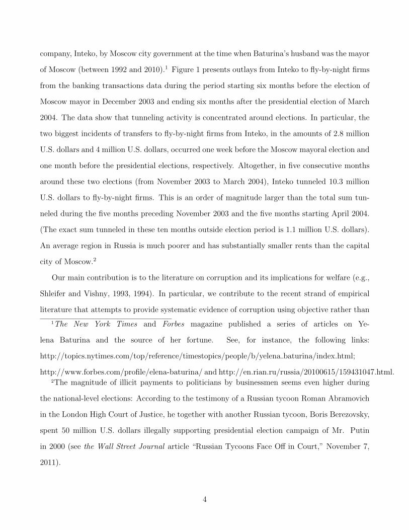
company, Inteko, by Moscow city government at the time when Baturina’s husband was the mayor

of Moscow (between 1992 and 2010).1 Figure 1 presents outlays from Inteko to fly-by-night firms

from the banking transactions data during the period starting six months before the election of

Moscow mayor in December 2003 and ending six months after the presidential election of March

2004. The data show that tunneling activity is concentrated around elections. In particular, the

two biggest incidents of transfers to fly-by-night firms from Inteko, in the amounts of 2.8 million

U.S. dollars and 4 million U.S. dollars, occurred one week before the Moscow mayoral election and

one month before the presidential elections, respectively. Altogether, in five consecutive months

around these two elections (from November 2003 to March 2004), Inteko tunneled 10.3 million

U.S. dollars to fly-by-night firms. This is an order of magnitude larger than the total sum tun-

neled during the five months preceding November 2003 and the five months starting April 2004.

(The exact sum tunneled in these ten months outside election period is 1.1 million U.S. dollars).

An average region in Russia is much poorer and has substantially smaller rents than the capital

city of Moscow.2

Our main contribution is to the literature on corruption and its implications for welfare (e.g.,

Shleifer and Vishny, 1993, 1994). In particular, we contribute to the recent strand of empirical

literature that attempts to provide systematic evidence of corruption using objective rather than

1The New York Times and Forbes magazine published a series of articles on Ye-

lena Baturina and the source of her fortune. See, for instance, the following links:

http://topics.nytimes.com/top/reference/timestopics/people/b/yelena baturina/index.html;

http://www.forbes.com/profile/elena-baturina/ and http://en.rian.ru/russia/20100615/159431047.html.2The magnitude of illicit payments to politicians by businessmen seems even higher during

the national-level elections: According to the testimony of a Russian tycoon Roman Abramovich

in the London High Court of Justice, he together with another Russian tycoon, Boris Berezovsky,

spent 50 million U.S. dollars illegally supporting presidential election campaign of Mr. Putin

in 2000 (see the Wall Street Journal article “Russian Tycoons Face Off in Court,” November 7,

2011).

4

perception-based measures (see, for instance, Di Tella and Schargrodsky, 2003; Reinikka and

Svensson, 2004; Bertrand, Djankov, Hanna and Mullainathan, 2007; Olken, 2007; Fisman and

Miguel, 2007; Butler, Fauver and Mortal, 2009; Caselli and Michaels, 2009; Cheung, Rau and

Stouraitis, 2011; Ferraz and Finan, 2011). We provide objective evidence of corruption in the

allocation of public procurement contracts for a comprehensive list of Russian large firms and

show that corruption exacerbates inefficiencies. Previous estimates of corruption were based on

perceptions or covered a much smaller segment of economic activity (see, for instance, work

surveyed by Bardhan, 1997; Rose-Ackerman, 1999; Svensson, 2005; Olken and Pande, 2012).

Our study is also related to the large body of work on corruption associated with political

connections (e.g., Fisman, 2001; Johnson and Mitton, 2003; Bertrand, Kramarz, Schoar and

Thesmar, 2007; Khwaja and Mian, 2005; Faccio, 2006; Faccio, Masulis and McConnell, 2006; Leuz

and Oberholzer-Gee, 2006). As is illustrated by the case of Inteko, political connections is one of

the mechanisms behind the evidence presented in this paper. Our study is particularly related

to the literature showing that political connections in part determine allocation of government

procurement contracts (e.g., Goldman, Rocholl and So, 2011; Amore and Bennedsen, 2010).3

We also contribute to the literature on opportunistic political cycles (see, for instance, a

survey by Drazen, 2001). This work focuses primarily on the correspondence between election

cycles and benefits directed to voters (in the form of transfers and social expenditure). We

document a political cycle in illegal cash payments that firms make to politicians in order to

obtain procurement contracts. Related to our findings, Burgess et al. (2012) show a political

cycle in another illegal activity which brings cash to politicians, namely, forest extraction in

the tropics. Our finding that firms provide benefits to politicians in the face of elections is

also related to Bertrand, Kramarz, Schoar and Thesmar (2007), who document that political

connections are associated with political cycle in employment granted for the political benefit of

3In addition, there is a related body of research which shows benefits of official campaign

financing for firms (e.g., Claessens, Feijen and Laeven, 2008; Cooper, Gulen and Ovtchinnikov,

2010).

5

incumbent politicians.

Our work is also related to the papers documenting political budget cycles for Russian gu-

bernatorial elections (Akhmedov and Zhuravskaya, 2004), state capture at the regional level in

Russia (Slinko, Yakovlev and Zhuravskaya, 2005; Guriev, Yakovlev and Zhuravskaya, 2010), and

tunneling by Russian firms (Desai, Dyck and Zingales, 2007; Mironov, 2013). Our work has some

methodological parallels with other papers which use unconventional data sources to provide em-

pirical evidence on the questions that cannot be studied using conventional data (e.g., Levitt and

Venkatesh, 2000; Guriev and Rachinsky, 2006; Braguinsky and Mityakov, Forthcoming; Braguin-

sky, Mityakov and Liscovich, 2011; Mironov, 2013, Forthcoming). Much of this work focuses on

Russia because of data availability.

The paper proceeds as follows. In section 2, we describe the data. Section 3 presents evidence

of a political cycle in illegal cash tunneled from companies that receive public procurement revenue

and estimates the size of illicit payments to politicians associated with obtaining procurement

contracts. Section 4 develops the methodology of measuring corruption using the association

between illicit payments and receiving procurement revenue across firms and presents a test of

this approach. In section 5, we use our measures of corruption show that corruption leads to

inefficiency in the allocation of public procurement. In section 6, we conclude.

2 Data

2.1 Legitimacy and Reliability of the Banking Transactions Data

Our main data source is the dataset used by Mironov (2013). It is the dataset of banking

transactions among legal entities in Russia between 1999 and 2004 allegedly leaked to the public

domain from the Russian Central Bank in 2005 and available freely on the Internet. These data are

available both for free and also for a symbolic payment from several websites: www.vivedata.com,

www.rusbd.com, www.wmbase.com, www.mos-inform.com, www.specsoft.info, etc. The Russian

6

press discussed widely the incident of appearance of these data in the public domain.4 The

websites that demand the symbolic payment primarily charge for the service they provided by

formatting the dataset to make the data more easily accessible rather than for the dataset itself,

as it is also available for free. As the data appeared in the public domain presumably without

an official permission of the Central Bank of Russia, it is important to note that the Russian

Government and Russian Central Bank are aware of the usage of these data by journalists and

researchers and publicly discuss policy-relevant conclusions of the analyses based on the data (see,

for instance, transcript of the Conference on Tax Evasion at the Ministry of Economy that took

place in October of 2006 in Moscow). In addition, the authors of this paper received a request

from the First Deputy Chairman of the Central Bank of Russia, Andrei Kozlov, and a Deputy

Chairman, Viktor Melnikov, to write a policy memo explaining the methodology of identifying

fly-by-night firms using the banking transactions data as developed by Mironov (2013). In this

request, the top Central Bank officials refer to “the data set from the Internet” as a legitimate

source of information and acknowledge that the research department of the Central Bank uses

the same data.5 The fact that the government and the Central Bank officials take the results of

research based on these data seriously is an indication of the reliability of these data.

As far as the legal issues associated with the use of these data are concerned, no lawsuits have

been initiated against any party for using these data in spite a fairly large circulation of the data

and publications by both journalists and researchers.6 Lawyers within the Ministry of Interior

of Russian Federation, when commenting in the press on the legitimacy of these data, explained

that the Russian Central Bank never admitted that any data were leaked from the Bank and,

4See, for instance, publication in the main Russian business daily Vedomosti on March 30,

2005.5A copy of the letter is available from the authors upon request.6For an example of a journalistic investigation using these data, see Vedomosti on May 20,

2005; for popular descriptions of research based on these data, see Vedomosti on July 24, 2006

and October 25, 2011. For research on similar datasets, see, for instance, Guriev and Rachinsky

(2006) and Braguinsky, Mityakov and Liscovich (2011).

7

therefore, from a legal standpoint, all data sets in the public domain are legal and no dataset is

considered as illegitimate.7

A detailed description of the data and several important reality checks on them were done

in Mironov (2013). These reality checks lead to the following conclusions. First, the Banking

Transactions data match rather well with the registry of Russian firms published by the Russia’s

official statistical agency Rosstat for the group of firms that actually pay taxes (i.e., legitimate

firms, as defined precisely in the next section, and used as a unit of observation in the analysis

that follows) and do not match for firms, which do not pay taxes (i.e., fly-by-nights, also as defined

in the next section). Second, for the firms that are present both in the Banking Transactions

data and the registry, firm characteristics – available in both data sets – exactly coincide, which

is another important sign of the reliability of the data.

2.2 Sample and Variables

The banking transactions data for 2003 and 2004 were used by Mironov (2013) and come from

www.vivedata.com. The data for 1999-2002 come from www.rusbd.com. The data set contains

513, 169, 660 transactions involving 1, 721, 914 business and government legal entities and self-

employed entrepreneurs without a legal enterprise status, with information on the date of each

transaction, its payer, recipient, the amount of each transaction, and the self-reported purpose of

it.

Our aim is to test for a relationship between transfers to fly-by-night firms from regular non-

government firms around elections, and the public procurements contracts that these regular

7See, for instance, Financial-economic news published by Interfaxon April 1, 2005. See also an

article, published in a journal specializing on covering the banking sector, Bankovskoye Obozreniye

(Banking Review), No. 11, November 2005, in which an economist from the Central Bank explains

the phenomenon of the leakage of these data by the excessive regulation of secrecy and the lack

of financial transparency regulations, he argues for the need to make the data officially public,

see http://bankir.ru/publikacii/s/provodki-cb-rf-vorovat-nelzya-pokypat-1378429/.

8

firms receive. Thus, the amounts of tunneling and public procurement revenue are the two main

variables in our analysis. Both of these variables are constructed from the list of banking trans-

actions. We describe how we construct these variables below. As for the sample of firms, we take

the universe of all entities present in the banking transaction data and eliminate all government

and municipal entities, all firms with 100% state or municipal ownership, all financial institutions,

all foreign companies and all self-employed entrepreneurs without a legal enterprise status. This

procedure eliminates little over 85% of all entities present in the Banking Transactions data. The

reminder is comprised of a near-population of domestic, non-financial, non-government business

legal entities, which are the focus of our analysis. As we describe below, we further narrow the

sample by eliminating firms of a small size, as they are both unlikely to get government procure-

ment contracts and unlikely to use services of fly-by-night firms, thus, they just add noise to our

estimation.

First, we follow Mironov (2013) and use these banking transactions data to measure the

amount of transfers to fly-by-night firms each week in each of the years between 1999 and 2004

for each regular firm in our sample. Mironov (2013) developed the methodology of identifying

fly-by-night firms, i.e., firms that have profitable banking transactions but pay no taxes, in the

banking transactions data set. Intuitively, fly-by-night firms are those that do not pay taxes

despite having transactions that require the payment of taxes according to Russian law. To be

precise, firms are defined as fly-by-night when they satisfy all of the following three criteria: (i)

the ratio of taxes paid to the difference in cash inflows and outflows is negligible (i.e., below

0.1%); (ii) social security taxes are below the amount which corresponds to the social security

tax for a firm with one employee on a minimum wage (i.e., $7.2); and (iii) cash inflows are higher

than cash outflows. In contrast to fly-by-night firms, regular (or legitimate) firms are commercial

entities that engage in commercial transactions and pay taxes. According to these criteria, we

identified 99,925 fly-by-night firms and 166,381 regular firms among the private business entities

in the banking transactions data. (Note that the vast majority of these regular firms are small

businesses.) For the purposes of this paper, we deem all the transfers from regular firms to the

9

fly-by-night firms as tunneling.

Second, we use the banking transactions data to identify revenue from public procurement

contracts for each firm in our sample of regular – i.e., legitimate – firms (described below). We

define revenue from public procurement contracts as the amount of all banking transactions

from government-affiliated entities to regular firms that have the reported purpose of “payment

for goods and services.” In the baseline analysis, we exclude payments for utilities such as

electricity and water from the list of revenues from public procurement contracts because the

utilities contracts are not usually allocated on a competitive basis and are automatically allocated

to local monopolists. The inclusion of utilities in the definition of public procurement does not

affect our results.

We also collect data on the basic characteristics of regular legitimate firms, such as location,

revenue, net income, debt, assets, and industry, which we use as control variables. Employment

data are available for a subset of these firms. These data come from the registry of Russian firms

published by the Russia’s official statistical agency (Rosstat). This is the most recent registry

that contains data on near-population of industrial firms in Russia in 2003. We merge regular

firms from the banking transaction database with the registry data.

Since we are interested in estimating the electoral cycle in tunneling, we focus on the 87

(out of 89) Russian regions that held gubernatorial elections between 1999 and 2004. The two

excluded regions are Dagestan, which has a parliamentary form of government, and Chechnya,

which experienced a severe armed conflict in 1999-2000. In the 87 regions, over the period under

study, 129 elections took place at 48 different points in time.

We construct our sample of regular firms by taking all firms that satisfy the following criteria

from these regions in their election years:

1. A firm should be present both in Rosstat’s 2003 registry and the banking transactions

database.

2. A firm’s revenue should be greater than $1M in 2003. We apply this criterion in order to

obtain a data set of manageable size and because one can reasonably expect relatively large

10

firms to engage in bribing in exchange for obtaining government procurement contracts. In

addition, the registry data can be considered as a near-population representative sample

only for large firms.

3. A firm should be active, i.e., it should have at least 10 transactions in the banking transac-

tions dataset over the entire period. As our measures of revenue from public procurement

contracts and of the transfers to fly-by-night firms are based on the banking transactions

data, we apply a minimum threshold for the number of transactions. We also require that

a firm should perform some banking transactions during a period one year before and one

year after the election.

These criteria yield 45, 275 regular firms. In order to assess the representativeness of the

sample, we compare the revenue of these firms to the total revenue generated by all Russian firms

(including the small ones, which are excluded from our sample). The total revenue of the firms

in our sample constitutes 73.1% of the total revenue for all firms in the Russian economy.

In the appendix, we present summary statistics for the entire sample (Table A.1) and sepa-

rately for each region (Table A.2). All nominal variables are expressed in thousands of constant

2003 U.S. dollars. A detailed description of variables can be found in the Data Appendix.

3 Political Cycle in Tunneling

3.1 Baseline estimation

Our first task is to estimate the electoral cycle in tunneling for firms with and without public

procurement contracts. We regress the tunneling that each firm in our sample makes each week

during the election year (between 1999 and 2004) normalized by the total amount of firm’s revenue

on a set of dummies indicating the time-distance to the election date, controlling for firm and week

fixed effects. We allow the electoral cycle to vary between two groups of firms: those which do

and do not receive substantial revenue from public procurement contracts, as we are interested in

the difference in the magnitude of the electoral cycle between the two groups. As larger firms may

11

have higher capacity to finance elections, we also allow for differential electoral cycles depending

on the size of firm’s revenue. The unit of analysis here is a firm in a particular week. Altogether

there are 6, 286, 011 firm-week observations in the sample, i.e., firm-weeks in each region in the

two years around each election among firms with non-zero transfers around elections (there are

45, 275 such firms). To be precise, we estimate the following equation:

TftRf

=30∑

w=−30

β1wDwGovfe+

30∑w=−30

β2wDw+

30∑w=−30

β3wDw log(Rf )+

2∑l=0

β4l log(If,t−l)+τt+φf +εft, (1)

where f indexes firms; t indexes time in weeks (there are 313 weeks over the entire time period

under study). The index w refers to the time-distance up to 30 weeks to the election date in

the region where the firm f is located, so that w = −1 refers to the week before the election

and w = 1 refers to the week after the election. As elections are always held on Sunday whereas

banking transactions occur during work days, w varies from −30 to −1 and then from 1 to 30

and is never equal to zero. Dw is the dummy indicating the week that is w weeks away from the

election date. Tft is the transfer by firm f to fly-by-night firms at time t. (T stands for tunneling).

Rf is the revenue of firm f in 2003. Subscript e indexes elections in a particular region. Thus,

it is redundant for all regions where there was only one election, and meaningful for regions

where there were two elections between 1999 and 2004. Govfe is a dummy which equals 1 if the

revenue from public procurement contracts as a share of the firm’s f total annualized revenue

+/- one year from the election e is greater than a certain threshold. As a baseline, we consider

the 5% threshold. To check the robustness of our results, we repeat the analysis redefining the

Govfe dummy as having 1% of revenue coming from public procurement contracts. log(Rf ) is

a measure of firm size, namely, the logarithm of the firm’s revenue in 2003.8 In addition, we

control for cash inflows into the firm bank account log(Ift) along with two lags of this variable.

8Due to data limitations, our sample size decreases dramatically if we control for revenue in

the election year rather than in 2003. The results are robust to this alteration. As a baseline, we

report results for the larger sample.

12

This control is needed to make sure that the timing of inflows is not driving our results on the

dynamics of outflows to fly-by-night firms. τt and φf are the full sets of 313 time and 45, 275

firm fixed effects. Our results are robust to excluding controls for the differential political cycle

depending on the size of the firm, i.e., Dw log(Rf ), and to excluding controls for cash inflows, i.e.,

log(If,t), log(If,t−1), and log(If,t−2). The main results (i.e., the coefficients β1w and β2

w) are also

unaffected by the choice of the threshold of revenue coming from procurement. The error term

εft is clustered at the level of each of 45, 275 firms.

In Specification 1, the differences between coefficients on Dw between weeks close to and far

away from election dates estimate the electoral cycle in tunneling for firms with procurement

revenue below the specified threshold (β2w). Our main coefficients of interest are β1

w, which

estimate the difference in the electoral cycles in tunneling between firms with procurement revenue

above and below the threshold.

In order to reduce idiosyncratic variation in the estimates of weekly frequency for presentation

purposes, we also estimate the coefficients on dummies indicating the proximity to elections at

monthly level. I.e., we re-estimate Equation 1 on the same sample, with the same controls, but

replacing 60 dummies Dw indicating week-distance from elections by 16 monthly dummies Dm,

where m indicates 4-week periods around elections. We estimate the following equation:

TftRf

=8∑

m=−8

β1mDmGovfe+

8∑m=−8

β2mDm+

8∑m=−8

β3mDm log(Rf )+

2∑l=0

β4l log(If,t−l)+τt+φf +εft, (2)

keeping the full set of 313 week fixed effects.

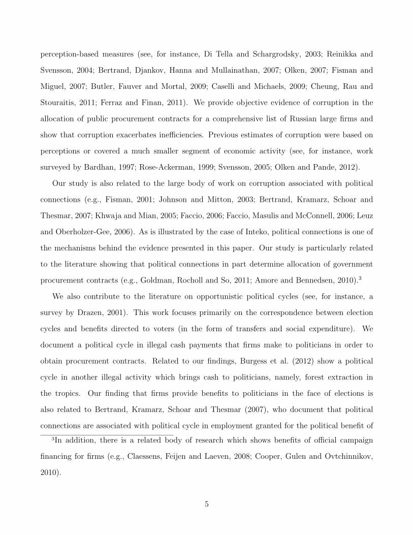
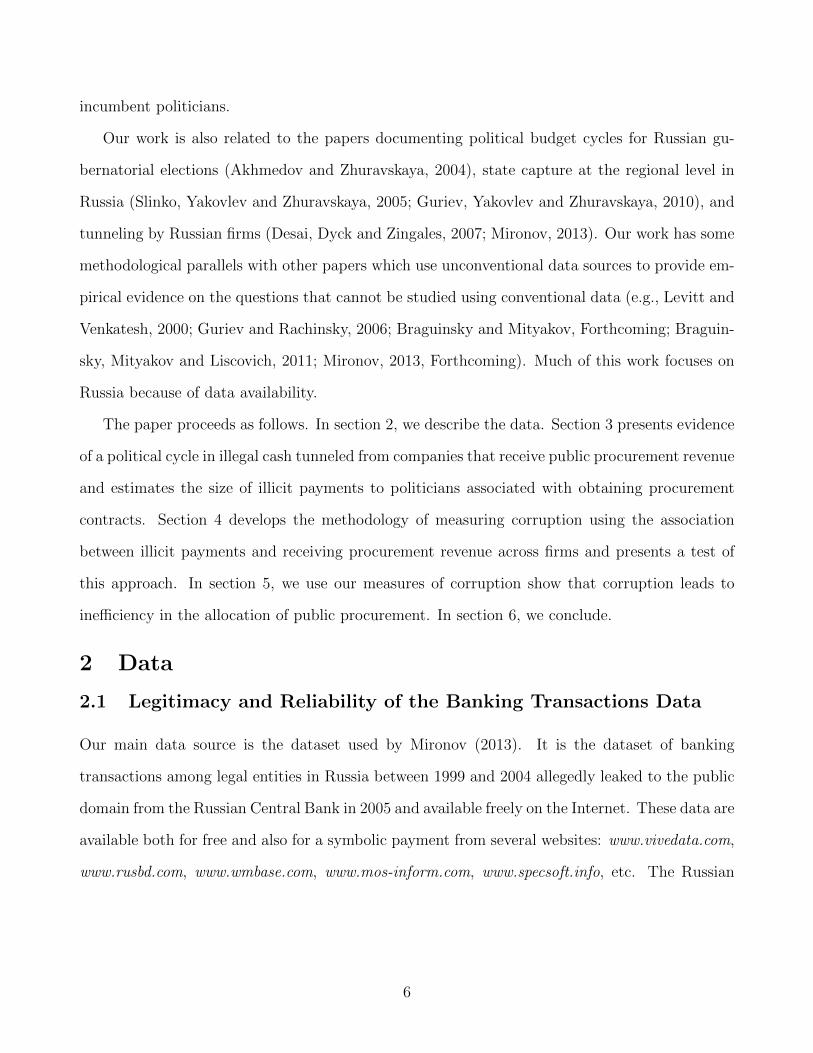
Figures 2 and 3 present the results of the estimations of Equations 1 and 2. The upper charts

portray the sum of point estimates of β1w and β2

w from Equation 1 by each week w around election

time on Figure 2 and the the sum of point estimates of β1m and β2

m from Equation 2 by each

month m; these estimates show the dynamics of the tunneling activity by firms with procurement

revenue above the 5% threshold at weekly and monthly frequency, respectively. Similarly, the

middle charts on the two figures portray the tunneling for firms with procurement revenue below

the 5% threshold, namely, β2w and β2

m coefficients. The lower charts show the difference between

13

the two, i.e., the estimates of β1w and β1

m. Each chart also portrays 95% confidence interval around

each estimated coefficient.

The two figures draw the same picture, but it is more visible on Figure 3 as the idiosyncratic

week-level variation is smoothed out using monthly averages. The graphs show that starting

approximately one half a year (24 weeks) before the election, firms start transferring more cash

to fly-by-night firms compared to their usual average tunneling activity at times when election is

far away (outside +/- 30 week period around elections). This increase in tunneling is present both

in firms with and without a large share of revenue coming from public procurement (the upper

and middle charts). However, it is particularly pronounced among firms with public procurement

above 5% of revenue threshold (the upper charts). The tunneling activity remains significantly

higher than usual for the entire 6 months prior to elections and grows steadily as elections

approach (see, in particular, Figure 3). However, the largest spike in the transfers to fly-by-

night firms occurs during the month right after the election. Starting from week +5 after the

election on, the tunneling activity falls to the usual level and fluctuates around it. The lower

charts demonstrate that the magnitude of the described political cycle is significantly higher

among firms with the sizable procurement revenue compared to firms with procurement below

the 5% threshold. Table A.3 in the Appendix presents the full regression output from estimating

Equation (1) along with the F -tests for the joint significance of all β-coefficients as well as F -tests

for the significance of the difference in the level of β-coefficients within the very short election

window of [-4; +4] weeks around elections compared to β-coefficients outside this election window.

All these F-tests yield statistical significance well above conventional levels.

In order to allow for the differential electoral cycle in tunneling, depending on the extent to

which firms rely on public procurement contracts for their business, we also estimate the following

two equations, first, with the political cycle estimated at the level of 60 weeks w around elections:

TftRf

=30∑

w=−30

γ1wDw

ProcRfe

Rf

+30∑

w=−30

γ2wDw+

30∑w=−30

γ3wDw log(Rf )+

2∑l=0

β4l log(If,t−l)+τt+φf+εft, (3)

14

and, second, at the level of 16 months m:

TftRf

=8∑

m=−8

γ1mDm

ProcRfe

Rf

+8∑

m=−8

γ2mDm+

8∑m=−8

γ3mDm log(Rf )+

2∑l=0

β4l log(If,t−l)+τt+φf+εft. (4)

The sample and the dependent variable are exactly as above. We just make one change to the set

of covariates. ProcRfe stands for the size of the firm’s procurement revenue +/- one year around

the election date (in annualized terms, i.e., divided by 2); and therefore,ProcRfe

Rfis the share of

annualized revenue from public procurement in the two years around elections as a fraction of the

firm’s total revenue as of 2003. The rest of the notation is as above. Again, to insure robustness,

we estimate these equations with and without controlling for the differential electoral cycle in

firms of different sizes, and with and without controls for cash inflows. The inclusion or exclusion

of these controls does not affect the main results. As above, the error terms are clustered at the

firm level. In Specifications 3 and 4, our main coefficients of interest are γ1w and γ1

m, respectively,

which estimate the additional electoral cycle in tunneling for an incremental increase in the share

of revenue coming from public procurement contracts.

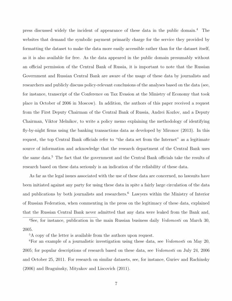
Figure 4 presents the point estimates of γ1w and γ1

m along with their confidence intervals in the

upper and lower charts, respectively. It shows that the magnitude of the political cycle increases

with an increase in the share of firm’s revenue coming from procurement contracts. This is the

case throughout the entire period of abnormal tunneling around elections, namely, from -6 to

+1 month around elections. Table A.4 in the Appendix presents the full regression output from

estimating Equation 3.

The magnitude of the incremental tunneling around elections is substantial. For example, dur-

ing one month after the elections, firms that get more than 5% of their revenue from procurement

contracts transfer to fly-by-night firms an additional sum equal to about 5.8% of their monthly

revenue (on top of the usual tunneling activity). For comparison, the usual tunneling activity for

an average (median) firm is about 4.75% (1.36%) of revenue. The increase in tunneling in half

a year before elections is also sizable. In 6 months prior to the election, firms with procurement

contracts above 5% of revenue increase their transfers to fly-by-night firms by the amount equal

15

to 1% to 3% of monthly revenue each month. For each additional percentage point of annual

revenue coming from the government procurement, the firms increase their tunneling by an addi-

tional amount equal to 0.16% of monthly revenue during one month right after the election, and

by an amount equal to 0.06%-0.08% of monthly revenue during the election campaign.

Overall, we find a strong evidence of a political cycle in transfers to fly-by-night firms which

is substantially and statistically significantly larger for firms with public procurement revenue.

3.2 Interpretation and the Effect of the Margin of Victory

Fly-by-night firms are used for tunneling, i.e., in order to transfer large sums into cash illegally

out of firms for various purposes, such as tax evasion and diverting cash from shareholders to

managers and from minority shareholders to majority shareholders (as in Johnson et al., 2000).

Mironov (2013) provides evidence that fly-by-night firms are usually registered on stolen passports

and do not provide any real services or produce any real goods. Instead, the legitimate firms sign

(from their standpoint) a perfectly legal contract with fly-by-night firms for “consulting services”

and pay them for these “services” via a banking transaction. Then, fly-by-night firms take the

cash out of the bank and give it back to the management of the legitimate firm (for a fee).9 All

tax liabilities associated with such banking transactions rest with the fly-by-night firms, whereas

the legitimate firms get the tunneled cash and is free to use it.

How one can explain the political cycle in tunneling? There are two potential explanations.

One is that abnormal levels tunneling around elections, indicate that the cash is transferred to

politicians. In that case, the fact that the tunneling increases during elections much more in

firms that rely on contracts with the government for their business suggests that these transfers

might be used as informal payments (i.e., bribes) for obtaining procurement contracts. The

second potential explanation is that firms tunnel cash out in the proximity of elections because

of a change in the political risk for firms associated with a possible change in the leadership.

9We cannot track what happens to the money after it was transferred to fly-by-night firms

precisely because it is cashed out, as we only observe banking transitions between legal entities.

16

The change in political risk could vary across firms, which would explain the differential cycle

between firms with and without procurement revenue. In this subsection, we argue that only the

first explanation is consistent with the evidence.

If the political risk is behind the political cycle in tunneling, one should expect the tunneling

around elections to be particularly high when elections yield the change in leadership, and there-

fore, the potential change in the formal regulatory environment or any informal implicit contracts

between the governor and the regional business. In contrast, if incumbent wins with a very large

margin of victory in the first round of elections, one should not expect any change in the rules

of the game between the business and the regional government, and therefore, these elections are

not associated with any additional political risk. Thus, in such elections, we should not observe

political cycle in tunneling, if the political risk is the mechanism driving the political cycle.

We test these predictions by exploring how the margin of victory and political turnover affect

the presence of the political cycle in tunneling during elections. In 27 out of 129 elections the

incumbent ran and lost. In 74 elections the winner got more than 50% of the total vote in the

first round of elections; and in 32 elections the incumbent got more than 70% of the total vote

in the first round of elections. We re-estimated the political cycle in tunneling using Equations

1-4 separately on the sub-samples of elections in which the winner got above and below 50%

of the vote in the first round, in which the incumbent lost and incumbent won, and finally in

which the incumbent got above and below 70% of the vote in the first round of elections. (We

also confirmed all of the results by estimating these equations on the full sample with additional

interaction terms allowing the cycle to differ between these groups of elections.)

We found that the political cycle in tunneling decreases sharply with an increase in political

competition, contrary to the prediction of the political risk mechanism. In particular, we do not

observe a statistically significant political cycle for elections in which the winner got less that

50% in the first round of elections and in which the incumbent lost. For the purposes of a concise

presentation of the results, we simplified the estimation further by replacing 60 Dw dummies

indicating distance to election in Equations 1 and 3 with just a single dummy indicating the

17

election window of [-4;+4] weeks around the election. We chose this window, as the deviation of

tunneling activity from the usual level is the highest during this time (as is evident from the results

of the estimation of the full cycle.) Table 1 summarizes these results, it reports coefficients on

the election window dummy and on the interaction between the election window dummy and the

dummy for procurement revenue above 5% of total revenue in upper panel, and on the interaction

between the election window dummy and the share of procurement in total revenue in the lower

panel. The results presented in the table confirm that there is no pronounced political cycle

in tunneling, even among firms with procurement revenue above 5% threshold, for elections, in

which the winner got less that 50% of the vote in the first round of elections and in which the

incumbent lost (see columns 1 and 3 of the upper panel of Table 1). The coefficients in the

second specification (lower panel) are more precisely estimated and, therefore, the coefficients on

the interaction between the size of procurement revenue share and the election window dummy

are statistically significant in this specification, even for the elections with a low margin of victory

(as reported in the lower panel of Table 1). Yet, their magnitude of the estimated coefficients of

interest is about 1/8th that for the subsample of elections with a larger margin of victory. The

magnitude of the cycle is exactly the same (and large) for elections, in which the winner got more

than 50% of the vote in the first round and those in which the incumbent won. Similar picture

emerges from the estimation of the political cycle for elections, in which incumbent got more and

less than 70% of the total vote in the first round of elections (see the last two columns of the

table). The magnitude of the political cycle for the elections, where the incumbent won with at

least 70% of the vote in the first round of election is substantially (2- to 4-times) larger than in

the rest of the sample.

Therefore, we conclude that the change in the political risk in the face of election cannot be

the driving force of the intensified tunneling around elections and that the reason for the political

cycle in tunneling is that the money are directed to politicians. The precise timing of the cycle

sheds some light on what these funds are used for. Out of the total amount of (abnormal)

tunneling activity of firms with public procurement revenue in the window starting 6 months

18

before elections and ending one month after elections, 2/3 of the cash is tunneled during the

election campaign preceding the election and 1/3 during one month after the election.

Politicians on the campaign trail are the ones who need cash the most in the face of elections.

Note that the law severely restricts the size of legal financing of election campaigns in Russia to

the point that the funds raised legally account for a tiny fraction of the total financing.10 Thus,

it is reasonable to conclude that the additional funds tunneled out of firms during the election

campaign of politically strong incumbents (for whom the political cycle in tunneling is at its

largest) are channeled to finance their campaigns. The strong correlation between the size of

procurement revenue and the tunneling during the election campaign suggests that such shadow

campaign financing is rewarded with procurement contracts.

It is possible that some of the campaign spending is realized also right after the elections,

as many campaign-related services (such as printing and distribution of advertisement leaflets,

T-shirts, or posters) are provided up until the very end of campaign. However, much of the

campaign spending (such as, for instance, vote-buying) is incurred on the spot, before the elec-

tion. The question, therefore, is why tunneling becomes the most intensive in the month right

after the election, when the election campaign is over. The answer was suggested to the authors

in an informal interview with public officials in the Moscow-city administration.11 Many of the

public procurement contracts are allocated for the time of the election term and, therefore, the

beginning of the electoral term is marked with new public procurement contracts being signed.

Again, the fact that illegal tunneling of cash intensifies during the time of signing public procure-

ment contracts suggests that the cash payments are used as bribes helping to get a procurement

10For example, according to expert estimates the pre-election budget of the United Russia

party for parliamentary election in 2003 was $250 million, whereas the maximum limit permitted

by the law was $8 million. For details, see the article in Novaya Gazeta, on September 18 2003

entitled “The biggest deal on the political market is the current parliamentary elections.”11Moscow city (along with one other metropolitan area of St. Petersburg) has a status of the

Subject of the Federation equal to the rest of Russia’s regions.

19

contract.12

In order to check the validity of our interpretation, we conduct two placebo experiments. First,

we test for the political cycle in transactions among legitimate regular firms in manufacturing

industries and find no evidence of such a cycle. This is an important test, as it rules out the

possibility that our results are driven by an unobserved increase in legitimate economic activity

around election time. Figure 5 illustrates the results. It portrays the dynamics of tunneling

(“shadow transfers”) and transfers to legitimate firms (“white transfers”) in industries unrelated

to publishing and media for our baseline sample of firms around election time, estimated using

Equation (1). It is evident from the figure that only illegitimate (“shadow”) transfers to fly-

by-night firms exhibit a political cycle. Transfers to the legitimate firms are completely flat

and do not depend on the proximity to elections. The table below the figure confirms that the

test for the equality of coefficients inside and outside the election window of [-4;4] weeks around

elections yields statistically significant difference only for transfers to fly-by-night firms and not

for transfers to legitimate firms. Thus, we conclude that the political cycle in tunneling is not

driven by a general increase in economic activity during the election time.

Furthermore, to make sure that our standard errors are not too small and our results are

not driven by some differential trends in regions or firms, we re-estimate cycle in tunneling using

Equations 1 and 3 for 200 randomly chosen combinations of placebo election dates in our regions.

We draw placebo election dates randomly from the time interval that our data cover, at least 16

weeks away from the true election dates. Figure 6 presents the histograms of F -statistic from the

test of equality of the means of coefficients of interest β1 and γ1) inside and outside the election

12We also explored whether the timing of the political cycle (namely, how much cash is tun-

neled before and how much after the election) depends on the margin of victory and found no

relationship. In addition, we analyzed how various regional characteristics affect the magnitude

of the cycle and found no robust correlations between the magnitude of the cycle with any of the

observable characteristics of the regions, with the exception of a positive association between the

cycle and perception-based measures of regional corruption, which we report below.

20

window (i.e., the tests for β1

w∈[−4;4] = β1

w*[−4;4] in the upper panel and γ1w∈[−4;4] = γ1

w*[−4;4] in

the lower panel of the graph). In each of the panels, the vertical line indicates the value of the

F -statistic for the same test performed on the true data, which is substantially larger than vast

majority of those generated by the placebo treatment. This experiment shows that the pattern in

the data that we uncover is very unlikely to be generated by a random realization or differential

trends between firms with and without government procurement revenue.

3.3 Magnitude

A simple unconditional difference-in-differences exercise can help illustrate the magnitude of the

phenomenon. Table 2 summarizes the average amount of transfers to fly-by-night firms per

firm in a two-by-two matrix. The rows display firms with and without any public procurement

contracts, and the columns display two time periods (an 8-week-long election window and an

average 8-week-long period outside the election window). As shown in the table, firms with

public procurement had larger tunneling both inside and outside the election window. This could

be explained by differences in firm size or corporate governance practices between the two groups

of firms. In addition, for both groups, tunneling inside the election window were larger than those

outside of it. This could be because politicians demand illicit cash contributions from all firms, for

example, in exchange for getting around various regulatory barriers to doing business (Yakovlev

and Zhuravskaya, 2013). The difference in tunneling inside and outside the election window,

however, was substantially larger for firms with public procurement: an average firm with public

procurement contracts tunneled 29, 940 USD more in a proximity to an average regional election.

An average region in Russia had 84 firms that received public procurement contracts. Thus,

the amount of illegal cash channeled to politicians around elections that is associated with dis-

tribution of public procurement in Russia was about 2.5 million USD.13 On average, firms that

tunnel cash around elections (i.e., those firms whose tunneling exhibits a political cycle) get about

13Regional elections in Russia were abolished in 2005. Since then regional governors have been

appointed by the Russia president rather than elected.

21

103, 000 USD more revenue from public procurement contracts per year than firms that do not

intensify their tunneling activity around elections. Therefore, a substantial part of these receipts

are likely to be returned to politicians as a kickback in the form of shadow election financing or

bribes right after the election.

4 Measuring the Extent of Corruption

So far, we documented that, on average, tunneling for firms that get public procurement contracts

follows a political cycle. The next question is whether we can measure corruption using the corre-

lation between tunneling around elections and allocation of government procurement. Our main

hypothesis is that the stronger association between the allocation of government procurement

contracts across firms with how much cash they tunneled during previous elections is an indica-

tion of higher level of corruption in government procurement. In order to test this hypothesis,

we need a measure of corruption which provides variation within Russia and does not come from

our data. The only available measure is the regional-level Corruption Perception Index of the

perceived corruption measured by the Transparency International-Russia foundation for 40 (out

of 89) regions in Russia.14 This is a perception-based index compiled using enterprise-managers

surveys; it was constructed only once, in 2002. For the purposes of simplicity of interpretation, we

take the z-score of the index, so that the resulting measure has zero mean and unit variance with

higher values indicating higher perceived regional corruption. With the help of this index, we can

test whether tunneling is more closely associated with winning public procurement contracts in

the regions named most corrupt by Transparency International.

For this purpose, and from now on, we consider a firm following a particular regional election

episode as the unit of analysis. Thus, our cross-section sample consists of all legitimate firms in

regions and years when elections took place.

First, we estimate the relationship between the probability of obtaining a procurement con-

tract in a year following a particular regional election by a particular regional firm and tunneling

14The index is available at url: http://www.anti-corr.ru/rating regions/index.htm.

22

activity of that firm during the preceding elections. Our main focus is on whether this relation-

ship is stronger in regions that a priori are considered more corrupt. More precisely, we estimate

the following linear probability model:

Prob[ProcRfe > 0] = α1L(TELfe ) + α2L(TELfe )× CPIf + α′3Xf + α4Sf + α5Mrf + τe + εfe. (5)

As a dependent variable we take the dummy indicating firms that received any revenue

from public procurement contracts in the year following a particular election e, i.e., firms with

ProcRfe > 0. (As shown in Table A.1, this dummy equals one in 17.11% of observations.)15

Our main explanatory variables of interest are the extent of tunneling actively of firm f during

election e (TELfe ) and the TI Regional Corruption Perception Index in the region where firm f is

located (CPIf ). TELfe denotes the average weekly transfer by firm f to fly-by-night firms within

the window of [-4; +4] weeks from the election date e in the region where firm f is located. TELfe

is measured in USD; and its distribution has a log-normal shape. To reduce the influence of

extreme values on our estimates, one needs to take logs of all such variables. However, tunneling

T can take the value of zero. Therefore, following MacKinnon and Magee (1990), instead of a log

function, we use the inverse hyperbolic sine function L(.), such that L(T ) = log(T + (T 2 + 1)1/2).

We use this transformation for all variables that can take the value of zero but should be logged.16

The main focus of our analysis is the coefficient α2 on the interaction between tunneling and the

TI corruption index, which shows whether the effect of tunneling on wining public procurement

contracts increases with the level of regional perceived corruption. Note that as the TI corruption

15The results are robust if we take procurement revenues +/- one year around elections, rather

than just for the year after the elections. We also verify that the results are robust to using

alternative thresholds of procurement revenue as a share of total revenue of 1% and 5% instead

of zero.16The results of regression analysis with L(T ) are easier interpreted than that with log(1 +T ),

as the estimated coefficients are approximately equal to percents, as if log(T ) was used. All our

results are robust to using log(1 + .) instead of L(.) transformations.

23

index does not vary over time, region fixed-effects control for the direct effect of regional variation

in perceived corruption.

Sf and Mrf are the industry (sector) and region dummies, which control for variation across

sectors and regions in public procurement contracts and in corruption. (r is the index for the

regions) τe is the year fixed effect controlling for multiple elections in a particular year. Xf is a

vector of additional control variables, namely, the logarithm of firm’s revenue, net income as a

share of revenue, and the ratio of debt to assets. All controls are measured in 2003.17 The error

term εfe is clustered at the level of firms.

The entire sample is comprised of 45, 275 firms (the same as in the previous section) and

63, 021 firm by election year observations. However, TI’s Regional CPI is available only for a

subset of regions. The inclusion of this variable decreases the sample size to 38, 044 firms and

54, 115 observations.

Further, in order to assess how perception index of corruption affects the association between

tunneling around elections and the size of procurement revenue that firms receive, we estimate an

additional specification, in which the dependent variable is the size of procurement revenue of firm

f in a year following election e as a share of firm’s revenue and the set of explanatory variables

is exactly as in Equation 5. Precisely, the dependent variable in this augmented specification is

L(ProcRfe), which is the the inverse hyperbolic sine transformation of ProcRfe. We verified that

the results are similar when the procurement revenue as share of total revenue (instead of the

absolute level) is taken as the dependent variable.

Table 3 presents the results. The first two columns report the results for the probability of

securing non-zero procurement revenue as dependent variable (as in equation 5), and the last two

columns - with the level of procurement revenue. In the first and the third column, we report

the average association between tunneling and procurement in the entire sample (which is the

17We verified that our results are robust to using contemporary rather than 2003 controls. The

sample, however, is substantially reduced when contemporary controls are included because of

data limitations. None of our main results depend on inclusion of a particular set of controls.

24

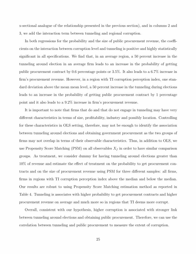
x-sectional analogue of the relationship presented in the previous section), and in columns 2 and

3, we add the interaction term between tunneling and regional corruption.

In both regressions for the probability and the size of public procurement revenue, the coeffi-

cients on the interaction between corruption level and tunneling is positive and highly statistically

significant in all specifications. We find that, in an average region, a 50 percent increase in the

tunneling around election in an average firm leads to an increase in the probability of getting

public procurement contract by 0.6 percentage points or 3.5%. It also leads to a 6.7% increase in

firm’s procurement revenue. However, in a region with TI corruption perception index, one stan-

dard deviation above the mean mean level, a 50 percent increase in the tunneling during elections

leads to an increase in the probability of getting public procurement contract by 1 percentage

point and it also leads to a 9.2% increase in firm’s procurement revenue.

It is important to note that firms that do and that do not engage in tunneling may have very

different characteristics in terms of size, profitability, industry and possibly location. Controlling

for these characteristics in OLS setting, therefore, may not be enough to identify the association

between tunneling around elections and obtaining government procurement as the two groups of

firms may not overlap in terms of their observable characteristics. Thus, in addition to OLS, we

use Propensity Score Matching (PSM) on all observables Xf in order to have similar comparison

groups. As treatment, we consider dummy for having tunneling around elections greater than

10% of revenue and estimate the effect of treatment on the probability to get procurement con-

tracts and on the size of procurement revenue using PSM for three different samples: all firms,

firms in regions with TI corruption perception index above the median and below the median.

Our results are robust to using Propensity Score Matching estimation method as reported in

Table 4. Tunneling is associates with higher probability to get procurement contracts and higher

procurement revenue on average and much more so in regions that TI deems more corrupt.

Overall, consistent with our hypothesis, higher corruption is associated with stronger link

between tunneling around elections and obtaining public procurement. Therefore, we can use the

correlation between tunneling and public procurement to measure the extent of corruption.

25

Our aim is to measure the degree of corruption in public procurement at the sub-regional

level in order to study the effect of corruption using with-region variation. We define localities

by the boundaries of sub-regional tax districts. We use this definition of localities because it is

easily observable using the codes of firm identifiers. The number of tax districts varies from 2

in a few smallest regions to 35 in the city of Moscow. Considering the extent of corruption in

procurement contracts at the level of locality is meaningful, as it is equivalent to small towns and

boroughs of large cities. A lot of public procurement contracts are allocated at this level. We

index localities with subscript l and estimate the specification analogous to Equation 5. However,

instead of the interaction between TI Corruption Perception Index and tunneling, we include a

set of interactions between dummies for each locality l (denoted by Dl) and tunneling around

elections as the main variables of interest (controlling for the unobserved variation across localities

with locality dummies):

Prob[ProcRfe > 0] =∑l

α1lDl × L(TELfe ) + α′2Xf + α3Sf + α4Dlf + τe + εfe. (6)

In order to estimate α1l precisely, we restrict the sample to localities with at least 40 firms, out of

which at least one has government procurement contracts. Using the results of this estimation,

we define two alternative measures of local corruption in allocation of public procurement: (1)

a dummy variable Cordl indicating that the estimate of α1l for the locality l is positive and

statistically significant at 10% level; and (2) a continuous measure Corcl equal to the magnitude

of the estimate of α1l irrespective of its statistical significance. Both measures are defined for 62

regions and 257 localities.18 Corcl varies across all localities in each region. Cordl equals zero in

every locality in 41 regions and there is a within-region variation in Cordl in 21 regions. Overall,

the coefficients α1l are positive and significant in 31% of localities.19 Summary statistics for these

variables are presented in Table A.5. The two measures of local corruption are complementary,

18For localities, where there are no private firms with procurement revenue (for instance, be-

cause government procurement contracts are allocated to state-owned or municipal firms), cor-

ruption in distribution of procurement revenue is undefined.19In a few cases, estimates of α1l are negative and significant at 5% level. However, this is well

26

as the first one has much larger variation and the second one is more precise. They are strongly

correlated with a pairwise correlation coefficient of 0.57, both also correlate with the TI Regional

Corruption Perception Index, with correlation coefficient of 0.74 for the dummy and 0.33 for the

continuos measure. The advantages of our measures over the TI measure are that they are based

on objective data; they are available at the sub-regional level; and for a much larger number of

regions. In the next section, we use these measures to test the “efficiency grease” hypothesis.

5 Does Corruption Contribute to Inefficiency?

Does corruption lead to an inefficiency in allocation of procurement contracts? Does it help or

hurt the chances of more efficient firms to gain public procurement? As the theoretical literature

provides reasons in favor of and against both possibilities, these are empirical questions. Our

measures of corruption can help to shed light on the answers. We use the variation in the level of

corruption across localities to test whether more or less efficient firms (other things held equal) are

more likely to obtain government procurement contracts in more corrupt localities. The challenge

is to measure efficiency across firms. The best available to us measure is revenue per worker (which

we consider to be an imperfect proxy for firm’s labor productivity). It is (unfortunately) available

only for a subset of the largest firms, so that the resulting data set consists of 19, 113 firms in

localities, where our corruption measures are defined. To test the “efficiency grease” hypothesis,

we regress a firm-level dummy for having won government procurement contracts above 1% of

total firm’s revenue on the measure of firms’ labor productivity, a measure of local corruption, and

their interaction, controlling for all our standard firm-level controls, as well as industry, region,

and year dummies:

Prob[ProcRfe

Rf

> 0.01] = δ1 log(yf )×Corlf + δ2Corlf + δ3 log(yf ) + δ′4Xf + δ5Sf + δ6Mf + τe+ εfe.

(7)

yf stands for the firm’s f labor productivity and Corlf is one of the two corruption measures

of locality l where firm f is located. Our main coefficient of interest is δ1; it estimates whether

within statistical error, as this occurs in 5.8% of the cases.

27

an increase in local corruption leads to a less or a more productive firm to get government

procurement contract. As the interaction term between local corruption and labor productivity

is identified even if we control for all unobserved heterogeneity among localities, we also estimate

a similar regression adding locality fixed effects (i.e., dummies for each locality: Dlf ) to the list

of controls and suppressing the direct effect of Corlf as it is collinear to locality effects:

Prob[ProcRfe

Rf

> 0.01] = δ1 log(yf )× Corlf + δ3 log(yfe) + δ′4Xf + δ5Sf + δ6Dlf + τe + εfe. (8)

Note that controlling for regional and industry fixed effects is crucial because a substantial vari-

ation in the amounts of procurement contracts and efficiency of firms are driven by unobserved

regional and industry-level factors. The results are presented in Table 5. The first four columns

present the estimation of Equation 7 and the last four columns – Equation 8. In every odd col-

umn, we suppress the interaction between the local corruption and labor productivity. Columns

1, 2, 5, and 6 use the continuous measure of corruption (i.e., α1 from Equation 6); columns 3, 4,

7, and 8 use the dummy for the significant α1 as the corruption measure.

First, we find that government procurement contracts are, on average, directed to firms with

lower revenue per worker (as the coefficient on labor productivity is negative and statistically

significant irrespective of specification). This result has two alternative interpretations. One

possibility is that the distribution of government procurement contracts is simply inefficient. The

alternative story, however, is that government procurement is distributed in order to support

higher employment for patronage reasons. The latter interpretation does not necessarily imply

lower efficiency as one can imagine two different technologies: one - more labor intensive and and

the other - less labor intensive. A paternalistic government with an objective of high employment

could chose firms with more labor intensive technology without an efficiency loss. The second

finding is our main focus: higher corruption is associated with less productive firms obtaining

public procurement contracts. The sign of the coefficients on the interaction term between labor

productivity and both of our corruption measures is negative in all specifications and statistically

28

significant in all but one specification.20 Importantly, in contrast to the interpretation of the

direct effect of yf , the interpretation of the effect of the interaction between yf and Corlf has an

unambiguous interpretation of an increase in the inefficiency in distribution of government pro-

curement contracts. This is because in more corrupt localities, by construction of our corruption

proxies, governments are less paternalistic on average as they distribute procurement contracts

in exchange for tunneling of illegal cash rather than in exchange for supporting higher levels of

employment. The magnitude of the effects is as follows: we find that in non-corrupt localities

government procurement contracts are allocated to firms which have 1.5% lower labor productiv-

ity compared to firms which do not win public procurement contracts in the same locality and

same industry. In contrast, in corrupt localities, firms with procurement revenue are 2.6% less

productive compared to non-recipients of public procurement contracts in the same locality and

same industry. Therefore, corruption leads to substantial efficiency losses in the allocation of

government procurement contracts. A plausible explanation of this results is that the managerial

qualities needed to bribe politicians and needed to run firms efficiently are substitutes rather than

compliments.

Overall, we reject the “efficient grease” hypothesis, as corruption leads to an increase in

inefficiency of distribution of public procurement contracts.

6 Conclusions

We use objective data for a near-population of Russian firms to develop a new methodology for

measuring corruption. Bribes follow a political cycle. Politicians collect bribes around elections

as an illicit payment for allocation of government procurement contracts. An average firm that

receives public procurement contracts pays about 30,000 U.S. dollars in bribes around a regional

election and gets procurement contracts that bring 100,000 U.S. dollars in additional revenue per

year. Using the correlation between tunneling around elections and the allocation of procurement

20The results are robust to using 0.1% rather than 1% threshold for the revenue coming from

public procurement contracts.

29

as a measure of corruption, we test and reject the “efficiency grease” hypothesis by showing that

less productive firms are more likely to win public procurement contracts in more corrupt localities

and, therefore, the allocation of public procurement is less efficient under corruption. Our findings

suggest that the managerial skills needed to run a firm efficiently do not help winning procurement

contracts in corrupt environments; and vice versa political capital that helps winning procurement

contracts does not help firm’s productivity.

References

Aidt, Toke S. 2003. “Review: Economic Analysis of Corruption: A Survey.” The EconomicJournal 113(491):pp. 632–652.

Akhmedov, Akhmed and Ekaterina Zhuravskaya. 2004. “Opportunistic Political Cycles: Test ina Young Democracy Setting.” Quarterly Journal of Economics 119(4):1301–1338.

Amore, Mario Daniele and Morten Bennedsen. 2010. “Political Reforms and the Causal Impact ofBlood - Related Politicians on Corporate Performance in the World’s Least Corrupt Society.”.Copenhagen Business School working paper, Copenhagen.

Bardhan, Pranab. 1997. “Corruption and Development: A Review of Issues.” Journal of EconomicLiterature 35:1320–1346.

Bertrand, Marianne, Francis Kramarz, Antoinette Schoar and David Thesmar. 2007. “PoliticallyConnected CEOs and Corporate Outcomes: Evidence from France.” Unpublished manuscript.

Bertrand, Marianne, Simeon Djankov, Rema Hanna and Sendhil Mullainathan. 2007. “Obtaininga Driver’s License in India: An Experimental Approach to Studying Corruption.” The QuarterlyJournal of Economics 122(4):1639–1676.

Braguinsky, Serguey and Sergey Mityakov. Forthcoming. “Foreign Corporations and the Cul-ture of Transparency: Evidence from Russian Administrative Data.” Journal of FinancialEconomics . http://papers.ssrn.com/sol3/papers.cfm?abstract id=1980581.

Braguinsky, Serguey, Sergey Mityakov and Andrey Liscovich. 2011. “Direct Estimation of HiddenEarnings: Evidence From Administrative Data.” Mimeo, John F. Kennedy School of Govern-ment.

Burgess, Robin, Matthew Hansen, Benjamin A. Olken, Peter Potapov and Stefanie Sieber. 2012.“The Political Economy of Deforestation in the Tropics.” Quarterly Journal of Economics127(4):1707–1754.

Butler, Alexander W., Larry Fauver and Sandra Mortal. 2009. “Corruption, Political Connections,and Municipal Finance.” Review of Financial Studies 22(7):2673–2705.

30

Caselli, Francesco and Guy Michaels. 2009. Do Oil Windfalls Improve Living Standards? Evidencefrom Brazil. NBER Working Papers 15550 National Bureau of Economic Research, Inc.

Cheung, Yan-Leung, Raghavendra Rau and Aris Stouraitis. 2011. “Which Firms Benefit fromBribes, and by How Much? Evidence From Corruption Cases Worldwide.” Mimeo, Hong KongBaptist University.

Claessens, Stijn, Erik Feijen and Luc Laeven. 2008. “Political Connections and PreferentialAccess to Finance: The Role of Campaign Contributions.” Journal of Financial Economics88(3):554–580.

Cooper, Michael J., Huseyin Gulen and Alexei V. Ovtchinnikov. 2010. “Corporate PoliticalContributions and Stock Returns.” Journal of Finance 65(2):687–724.

Desai, Mihir A., Alexander Dyck and Luigi Zingales. 2007. “Theft and taxes.” Journal of Finan-cial Economics 84(3):591–623.

Di Tella, Rafael and Ernesto Schargrodsky. 2003. “The Role of Wages and Auditing duringa Crackdown on Corruption in the City of Buenos Aires.” Journal of Law and Economics46(1):269–92.

Drazen, Allan. 2001. The Political Business Cycle After 25 Years. In NBER MacroeconomicsAnnual 2000, Volume 15. NBER Chapters National Bureau of Economic Research, Inc pp. 75–138.

Faccio, Mara. 2006. “Politically Connected Firms.” American Economic Review 96(1):369–386.

Faccio, Mara, Ronald Masulis and John J. McConnell. 2006. “Political Connections and CorporateBailouts.” Journal of Finance 61(6):2597–2635.

Ferraz, Claudio and Frederico Finan. 2008. “Exposing Corrupt Politicians: The Effects ofBrazil’s Publicly Released Audits on Electoral Outcomes.” The Quarterly Journal of Economics123(2):703–745.

Ferraz, Claudio and Frederico Finan. 2011. “Electoral Accountability and Corruption: Evidencefrom the Audits of Local Governments.” American Economic Review 101(4):1274–1311.

Fisman, Raymond. 2001. “Estimating the Value of Political Connections.” American EconomicReview 91(4):1095–1102.

Fisman, Raymond and Edward Miguel. 2007. “Corruption, Norms, and Legal Enforcement:Evidence from Diplomatic Parking Tickets.” Journal of Political Economy 115(6):1020–1048.

Goldman, Eitan, Jorg Rocholl and Jongil So. 2011. “Political Connections and the Allocation ofProcurement Contracts.” Mimeo, Indiana University.

Guriev, Sergei and Andrei Rachinsky. 2006. The Evolution of Personal Wealth in the FormerSoviet Union and Central and Eastern Europe. Working Papers RP2006/120 World Institutefor Development Economic Research (UNU-WIDER).

31

Guriev, Sergei, Evgeny Yakovlev and Ekaterina Zhuravskaya. 2010. “Interest Group Politics in aFederation.” Journal of Public Economics 94:730–748.

Huntington, Samuel P. 1968. Political Order in Changing Societies. New Haven: Yale UniversityPress.

Johnson, Simon, Rafael La Porta, Florencio Lopez de Silanes and Andrei Shleifer. 2000. “Tun-neling.” American Economic Review 90(2):22–27.

Johnson, Simon and Todd Mitton. 2003. “Cronyism and Capital Controls: Evidence fromMalaysia.” Journal of Financial Economics 67:351–382.

Khwaja, Asim Ijaz and Atif Mian. 2005. “Do Lenders Favor Politically Connected Firms? RentProvision in an Emerging Financial Market.” Quarterly Journal of Economics 120(4):1371–1411.

Leff, Nathaniel H. 1964. “Economic Development through Bureaucratic Corruption.” The Amer-ican Behavioral Scientist 8(2):8–14.

Leuz, Christian and Felix Oberholzer-Gee. 2006. “Political relationships, global financing, andcorporate transparency: Evidence from Indonesia.” Journal of Financial Economics 81(2):411–439.

Levitt, Steven D. and Sudhir Alladi Venkatesh. 2000. “An Economic Analysis Of A Drug-SellingGang’S Finances.” The Quarterly Journal of Economics 115(3):755–789.

MacKinnon, James G and Lonnie Magee. 1990. “Transforming the Dependent Variable in Re-gression Models.” International Economic Review 31(2):315–39.

Mironov, Maxim. 2013. “Taxes, Theft, and Firm Performance.” Journal of Finance 68(4):1441–1472.

Mironov, Maxim. Forthcoming. “Should One Hire a Corrupt CEO in a Corrupt Country?” Jour-nal of Financial Economics . http://papers.ssrn.com/sol3/papers.cfm?abstract id=2023988.

Olken, Benjamin A. 2006. “Corruption and the Costs of Redistribution: Micro Evidence fromIndonesia.” Journal of Public Economics 90(4-5):853–870.

Olken, Benjamin A. 2007. “Monitoring Corruption: Evidence from a Field Experiment in In-donesia.” Journal of Political Economy 115:200–249.

Olken, Benjamin A. and Rohini Pande. 2012. “Corruption in Developing Countries.” AnnualReview of Economics 4(1):479–509.

Reinikka, Ritva and Jakob Svensson. 2004. “Local Capture: Evidence from a Central GovernmentTransfer Program in Uganda.” Quarterly Journal of Economics 119(2):679–705.

Reinikka, Ritva and Jakob Svensson. 2006. “Using Micro-Surveys to Measure and Explain Cor-ruption.” World Development 34(2):359–370.

32

Rose-Ackerman, Susan. 1999. Corruption: Causes, Consequences, and Reform. Cambridge:Cambridge University Press.

Shleifer, Andrei and Robert W. Vishny. 1993. “Corruption.” Quarterly Journal of Economics108(3):599–617.

Shleifer, Andrei and Robert W. Vishny. 1994. “Politicians and Firms.” Quarterly Journal ofEconomics 109(4):995–1025.

Slinko, Irina, Evgeny Yakovlev and Ekaterina Zhuravskaya. 2005. “Laws for Sale: Evidence fromRussian Regions.” American Law and Economics Review 7(1):284–318.

Svensson, Jakob. 2005. “Eight Questions about Corruption.” Journal of Economic Perspectives19(3):19–42.

Yakovlev, Evgeny and Ekaterina Zhuravskaya. 2013. “The Unequal Enforcement of Liberalization:Evidence from Russia’s Reform of Business Regulation.” Journal of the European EconomicAssociation 11(4):808–838.

33

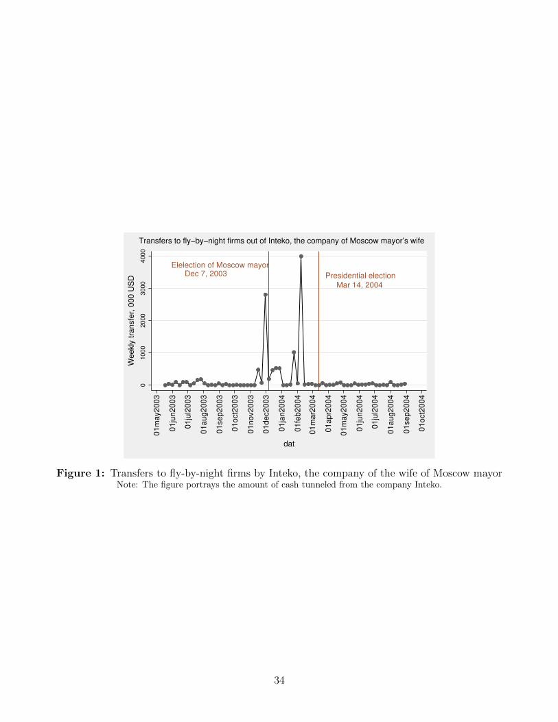
Elelection of Moscow mayorDec 7, 2003 Presidential election

Mar 14, 2004

01

00

02

00

03

00

04

00

0

Weekly

tra

nsfe

r, 0

00 U

SD

01m

ay2003

01ju

n2003

01ju

l2003

01aug2003

01sep2003

01oct2

003

01nov2003

01dec2003

01ja

n2004

01fe

b2004

01m

ar2

004

01apr2

004

01m

ay2004

01ju

n2004

01ju

l2004

01aug2004

01sep2004

01oct2

004

dat

Transfers to fly−by−night firms out of Inteko, the company of Moscow mayor’s wife

Figure 1: Transfers to fly-by-night firms by Inteko, the company of the wife of Moscow mayorNote: The figure portrays the amount of cash tunneled from the company Inteko.

34

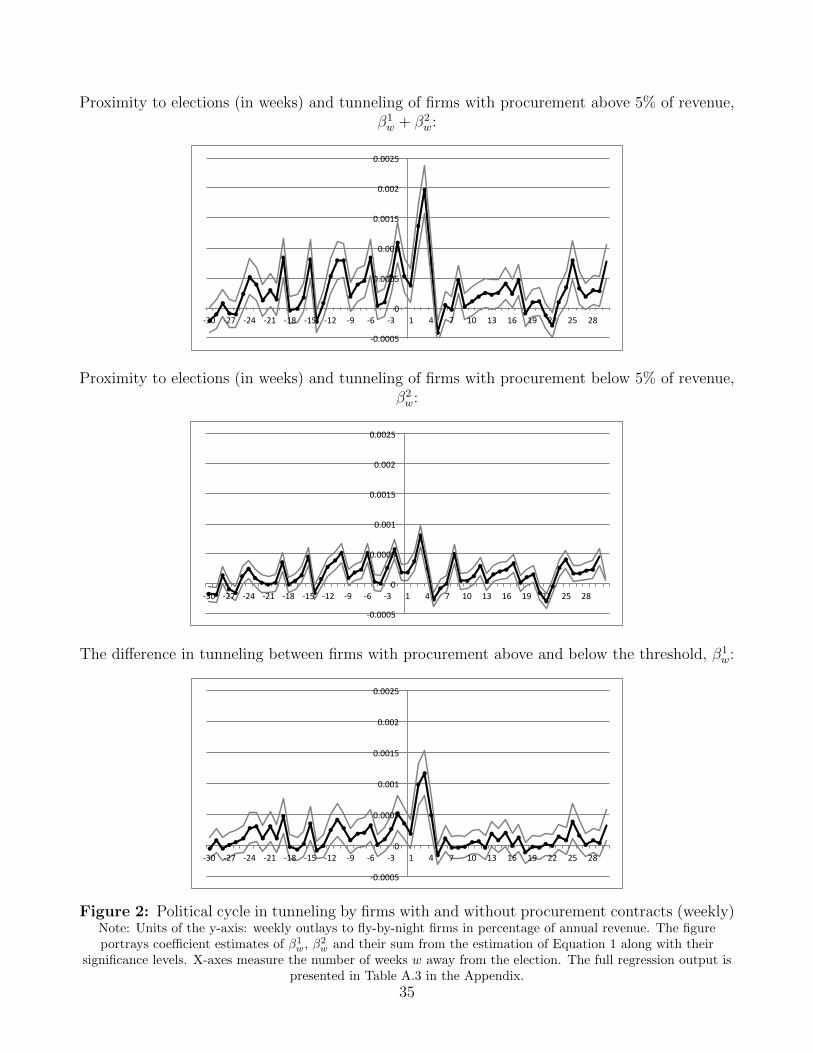
Proximity to elections (in weeks) and tunneling of firms with procurement above 5% of revenue,β1w + β2

w:

-­‐0.0005  

0  

0.0005  

0.001  

0.0015  

0.002  

0.0025  

-­‐30   -­‐27   -­‐24   -­‐21   -­‐18   -­‐15   -­‐12   -­‐9   -­‐6   -­‐3   1   4   7   10   13   16   19   22   25   28  

Proximity to elections (in weeks) and tunneling of firms with procurement below 5% of revenue,β2w:

-­‐0.0005  

0  

0.0005  

0.001  

0.0015  

0.002  

0.0025  

-­‐30   -­‐27   -­‐24   -­‐21   -­‐18   -­‐15   -­‐12   -­‐9   -­‐6   -­‐3   1   4   7   10   13   16   19   22   25   28  

The difference in tunneling between firms with procurement above and below the threshold, β1w:

-­‐0.0005  

0  

0.0005  

0.001  

0.0015  

0.002  

0.0025  

-­‐30   -­‐27   -­‐24   -­‐21   -­‐18   -­‐15   -­‐12   -­‐9   -­‐6   -­‐3   1   4   7   10   13   16   19   22   25   28  

Figure 2: Political cycle in tunneling by firms with and without procurement contracts (weekly)Note: Units of the y-axis: weekly outlays to fly-by-night firms in percentage of annual revenue. The figureportrays coefficient estimates of β1

w, β2w and their sum from the estimation of Equation 1 along with their

significance levels. X-axes measure the number of weeks w away from the election. The full regression output ispresented in Table A.3 in the Appendix.

35

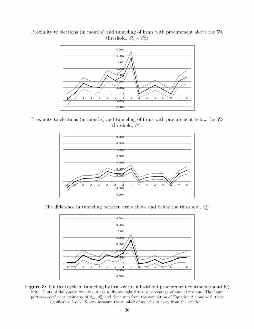
Proximity to elections (in months) and tunneling of firms with procurement above the 5%threshold, β1

m + β2m:

-­‐0.0004  

-­‐0.0002  

0  

0.0002  

0.0004  

0.0006  

0.0008  

0.001  

0.0012  

0.0014  

-­‐8   -­‐7   -­‐6   -­‐5   -­‐4   -­‐3   -­‐2   -­‐1   1   2   3   4   5   6   7   8  

Proximity to elections (in months) and tunneling of firms with procurement below the 5%threshold, β2

m:

-­‐0.0004  

-­‐0.0002  

0  

0.0002  

0.0004  

0.0006  

0.0008  

0.001  

0.0012  

0.0014  

-­‐8   -­‐7   -­‐6   -­‐5   -­‐4   -­‐3   -­‐2   -­‐1   1   2   3   4   5   6   7   8  

The difference in tunneling between firms above and below the threshold, β1m:

-­‐0.0004  

-­‐0.0002  

0  

0.0002  

0.0004  

0.0006  

0.0008  

0.001  

0.0012  

0.0014  

-­‐8   -­‐7   -­‐6   -­‐5   -­‐4   -­‐3   -­‐2   -­‐1   1   2   3   4   5   6   7   8  

Figure 3: Political cycle in tunneling by firms with and without procurement contracts (monthly)Note: Units of the y-axis: weekly outlays to fly-by-night firms in percentage of annual revenue. The figureportrays coefficient estimates of β1

m, β2m and their sum from the estimation of Equation 2 along with their

significance levels. X-axes measure the number of months m away from the election.

36

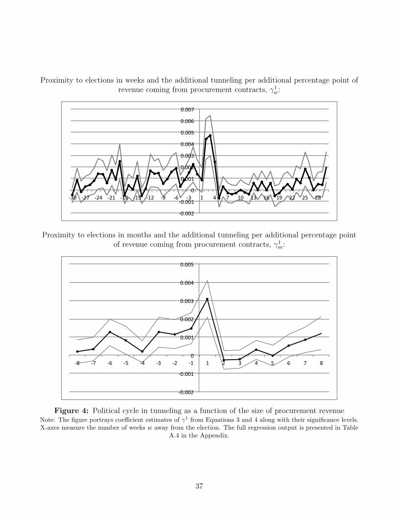
Proximity to elections in weeks and the additional tunneling per additional percentage point ofrevenue coming from procurement contracts, γ1

w:

-­‐0.002  

-­‐0.001  

0  

0.001  

0.002  

0.003  

0.004  

0.005  

0.006  

0.007  

-­‐30   -­‐27   -­‐24   -­‐21   -­‐18   -­‐15   -­‐12   -­‐9   -­‐6   -­‐3   1   4   7   10   13   16   19   22   25   28  

Proximity to elections in months and the additional tunneling per additional percentage pointof revenue coming from procurement contracts, γ1

m:

-­‐0.002  

-­‐0.001  

0  

0.001  

0.002  

0.003  

0.004  

0.005  

-­‐8   -­‐7   -­‐6   -­‐5   -­‐4   -­‐3   -­‐2   -­‐1   1   2   3   4   5   6   7   8  

Figure 4: Political cycle in tunneling as a function of the size of procurement revenueNote: The figure portrays coefficient estimates of γ1 from Equations 3 and 4 along with their significance levels.X-axes measure the number of weeks w away from the election. The full regression output is presented in Table

A.4 in the Appendix.

37

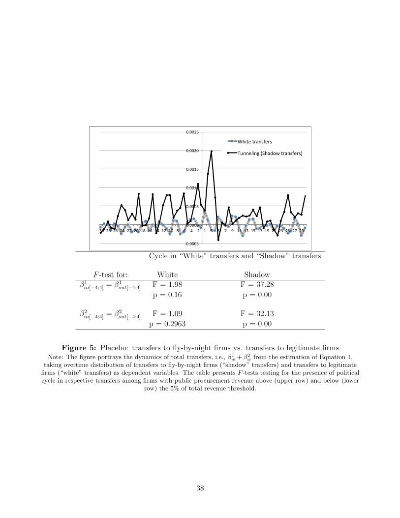
-­‐0.0005  

0.0000  

0.0005  

0.0010  

0.0015  

0.0020  

0.0025  

-­‐30  -­‐28  -­‐26  -­‐24  -­‐22  -­‐20  -­‐18  -­‐16  -­‐14  -­‐12  -­‐10   -­‐8   -­‐6   -­‐4   -­‐2   1   3   5   7   9   11   13   15   17   19   21   23   25   27   29  

White  transfers  

Tunneling  (Shadow  transfers)  

Cycle in “White” transfers and “Shadow” transfers

F -test for: White Shadowβ1in[−4;4] = β1

out[−4;4] F = 1.98 F = 37.28

p = 0.16 p = 0.00

β2in[−4;4] = β2

out[−4;4] F = 1.09 F = 32.13

p = 0.2963 p = 0.00

Figure 5: Placebo: transfers to fly-by-night firms vs. transfers to legitimate firmsNote: The figure portrays the dynamics of total transfers, i.e., β1

w + β2w from the estimation of Equation 1,

taking overtime distribution of transfers to fly-by-night firms (“shadow” transfers) and transfers to legitimatefirms (“white” transfers) as dependent variables. The table presents F -tests testing for the presence of politicalcycle in respective transfers among firms with public procurement revenue above (upper row) and below (lower

row) the 5% of total revenue threshold.

38

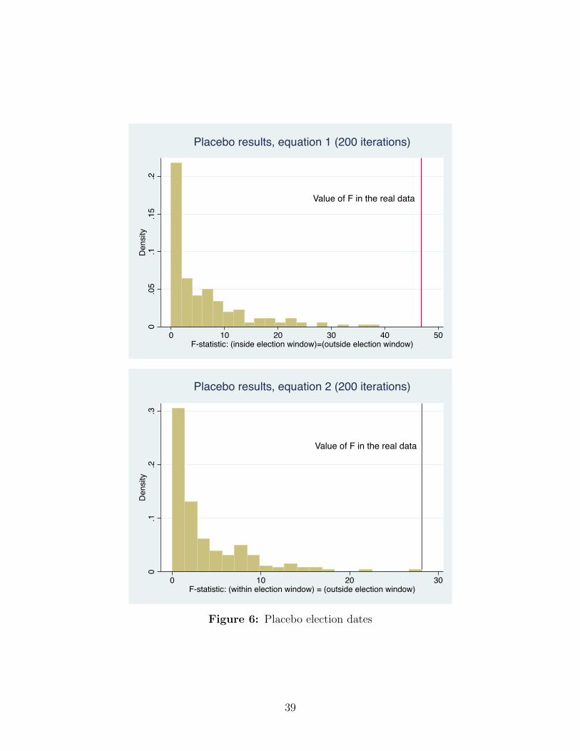
0.0

5.1

.15

.2D

ensi

ty

0 10 20 30 40 50F-statistic: (inside election window)=(outside election window)

Value of F in the real data

Placebo results, equation 1 (200 iterations)0

.1.2

.3D

ensi

ty

0 10 20 30F-statistic: (within election window) = (outside election window)

Value of F in the real data

Placebo results, equation 2 (200 iterations)

Figure 6: Placebo election dates

39

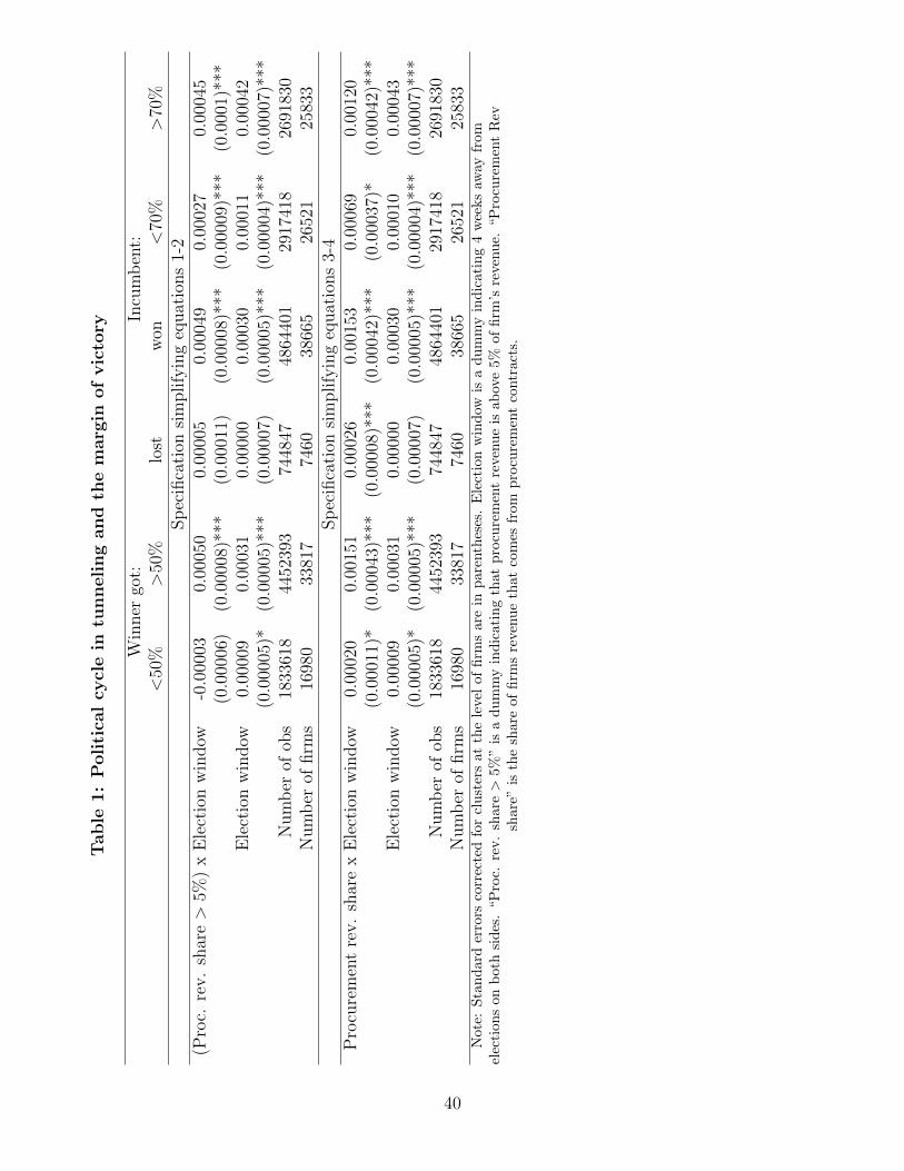
Table

1:

Poli

tica

lcy

cle

intu

nneli

ng

and

the

marg

inof

vic

tory

Win

ner

got:

Incu

mb

ent:

<50

%>

50%

lost

won

<70

%>

70%

Sp

ecifi

cati

onsi

mplify

ing

equat

ions

1-2

(Pro

c.re

v.

shar

e>

5%)

xE

lect

ion

win

dow

-0.0

0003

0.00

050

0.00

005

0.00

049

0.00

027

0.00

045

(0.0

0006

)(0

.000

08)*

**(0

.000

11)

(0.0

0008

)***

(0.0

0009

)***

(0.0

001)

***

Ele

ctio

nw

indow

0.00

009

0.00

031

0.00

000

0.00

030

0.00

011

0.00

042

(0.0

0005

)*(0

.000

05)*

**(0

.000

07)

(0.0

0005

)***

(0.0

0004

)***

(0.0

0007

)***

Num

ber

ofob

s18

3361

844

5239

374

4847

4864

401

2917

418

2691

830

Num

ber

offirm

s16

980

3381

774

6038

665

2652

125

833

Sp

ecifi

cati

onsi

mplify

ing

equat

ions

3-4

Pro

cure

men

tre

v.

shar

ex

Ele

ctio

nw

indow

0.00

020

0.00

151

0.00

026

0.00

153

0.00

069

0.00

120

(0.0

0011

)*(0

.000

43)*

**(0

.000

08)*

**(0

.000

42)*

**(0

.000

37)*

(0.0

0042

)***

Ele

ctio

nw

indow

0.00

009

0.00

031

0.00

000

0.00

030

0.00

010

0.00

043

(0.0

0005

)*(0

.000

05)*

**(0

.000

07)

(0.0

0005

)***

(0.0

0004

)***

(0.0

0007

)***

Num

ber

ofob

s18

3361

844

5239

374

4847

4864

401

2917

418

2691

830

Num

ber

offirm

s16

980

3381

774

6038

665

2652

125

833

Not

e:S

tan

dar

der

rors

corr

ecte

dfo

rcl

ust

ers

at

the

leve

lof

firm

sare

inp

are

nth

eses

.E

lect

ion

win

dow

isa

du

mm

yin

dic

ati

ng

4w

eeks

away

from

elec

tion

son

bot

hsi

des

.“P

roc.

rev.

shar

e>

5%”

isa

du

mm

yin

dic

ati

ng

that

pro

cure

men

tre

venu

eis

ab

ove

5%of

firm

’sre

venue.

“P

rocu

rem

ent

Rev

shar

e”is

the

share

of

firm

sre

venu

eth

at

com

esfr

om

pro

cure

men

tco

ntr

acts

.

40

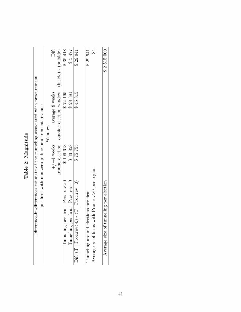
Table

2:

Magnit

ude

Diff

eren

ce-i

n-d

iffer

ence

ses

tim

ate

ofth

etu

nnel

ing

asso

ciat

edw

ith

pro

cure

men

tp

erfirm

wit

hnon

-zer

opublic

pro

cure

men

tre

venue

Win

dow

:+

/−4

wee

ks

aver

age

8w

eeks

Dif

:ar

ound

elec

tion

outs

ide

elec

tion

win

dow

(insi

de)

-(o

uts

ide)

Tunnel

ing

per

firm|P

roc.

rev>

0$

109

613

$74

195

$35

418

Tunnel

ing

per

firm|P

roc.

rev=

0$

3385

8$

2838

1$

547

7D

if:

(T|P

roc.

rev>

0)-

(T|P

roc.

rev=

0)$

7575

5$

4581

5$

2994

1

Tunnel

ing

arou

nd

elec

tion

sp

erfirm

$29

941

Ave

rage

#of

firm

sw

ith

Pro

c.re

v>

0p

erre

gion

84

Ave

rage

size

oftu

nnel

ing

per

elec

tion

$2

515

000

41

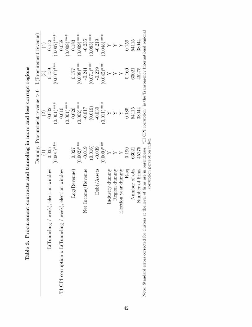
Table

3:

Pro

cure

ment

contr

act

sand

tunneli

ng

inm

ore

and

less

corr

up

tre

gio

ns

Dum

my:

Pro

cure

men

tre

venue>

0L

(Pro

cure

men

tre

venue)

(1)

(2)

(3)

(4)

L(T

unnel

ing

/w

eek),

elec

tion

win

dow

0.03

50.

032

0.15

90.

142

(0.0

01)*

**(0

.001

)***

(0.0

07)*

**(0

.007

)***

TI

CP

Ico

rrupti

onx

L(T

unnel

ing

/w

eek),

elec

tion

win

dow

0.01

00.

058

(0.0

01)*

**(0

.008

)***

Log

(Rev

enue)

0.02

70.

026

0.17

70.

183

(0.0

02)*

**(0

.002

)***

(0.0

08)*

**(0

.009

)***

Net

Inco

me/

Rev

enue

-0.0

19-0

.017

-0.2

41-0

.235

(0.0

16)

(0.0

19)

(0.0

71)*

**(0

.083

)***

Deb

t/A

sset

s-0

.039

-0.0

39-0

.219

-0.2

19(0

.009

)***

(0.0

11)*

**(0

.042

)***

(0.0

48)*

**In

dust

rydum

my

YY

YY

Reg

ion

dum

my

YY

YY

Ele

ctio

nye

ardum

my

YY

YY

R-s

q0.

190

0.18

50.

160

0.15

9N

um

ber

ofob

s63

021

5411

563

021

5411

5N

um

ber

offirm

s45

275

3804

445

275

3804

4N

ote:

Sta

nd

ard

erro

rsco

rrec

ted

for

clu

ster

sat

the

leve

lof

firm

sare

inp

are

nth

eses

.“T

IC

PI

corr

up

tion

”is

the

Tra

nsp

are

ncy

Inte

rnati

on

al

regio

nal

corr

up

tion

per

cep

tion

ind

ex.

42

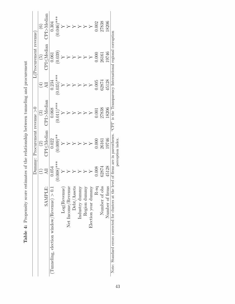
Table

4:

Pro

pen

sity

scor

ees

tim

ates

ofth

ere

lati

onsh

ipb

etw

een

tunnel

ing

and

pro

cure

men

t

Dum

my:

Pro

cure

men

tre

venue>

0L

(Pro

cure

men

tre

venue)

(1)

(2)

(3)

(4)

(5)

(6)

SA

MP

LE

:A

llC

PI≤

Med

ian

CP

I>M

edia

nA

llC

PI≤

Med

ian

CP

I>M

edia

n(T

unnel

ing,

elec

tion

win

dow

/Rev

enue)>

0.1

0.05

40.

022

0.06

80.

234

0.06

10.

304

(0.0

08)*

**(0

.009

)**

(0.0

11)*

**(0

.035

)***

(0.0

39)

(0.0

46)*

**L

og(R

even

ue)

YY

YY

YY

Net

Inco

me/

Rev

enue

YY

YY

YY

Deb

t/A

sset

sY

YY

YY

YIn

dust

rydum

my

YY

YY

YY

Reg

ion

dum

my

YY

YY

YY

Ele

ctio

nye

ardum

my

YY

YY

YY

R-s

q0.

008

0.00

00.

001

0.00

50.

000

0.00

2N

um

ber

ofob

s62

874

2616

127

838

6287

426

161

2783

8N

um

ber

offirm

s45

128

1974

618

206

4512

819

746

1820

6N

ote:

Sta

nd

ard

erro

rsco

rrec

ted

for

clu

ster

sat

the

leve

lof

firm

sare

inp

are

nth

eses

.“C

PI”

isth

eT

ran

spare

ncy

Inte

rnati

on

al

regio

nal

corr

up

tion

per

cep

tion

ind

ex.

43

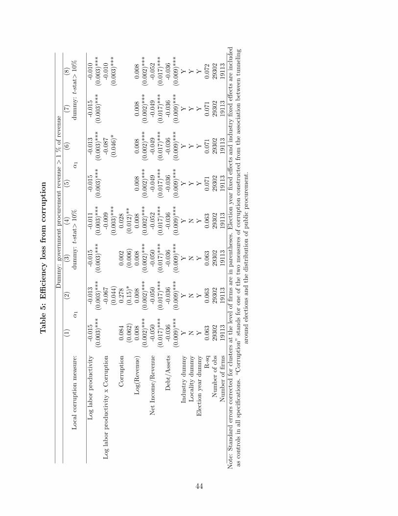
Table

5:

Effi

ciency

loss

from

corr

upti

on

Du

mm

y:

gov

ern

men

tp

rocu

rem

ent

reve

nu

e>

1%

of

reve

nu

e(1

)(2

)(3

)(4

)(5

)(6

)(7

)(8

)L

oca

lco

rru

pti

onm

easu

re:

α1

du

mm

y:t-

stat>

10%

α1

du

mm

y:t-

stat>

10%

Log

lab

orp

rod

uct

ivit

y-0

.015

-0.0

13

-0.0

15

-0.0

11

-0.0

15

-0.0

13

-0.0

15

-0.0

10

(0.0

03)*

**

(0.0

03)*

**

(0.0

03)*

**

(0.0

03)*

**

(0.0

03)*

**

(0.0

03)*

**

(0.0

03)*

**

(0.0

03)*

**

Log

lab

orp

rod

uct

ivit

yx

Cor

rup

tion

-0.0

67

-0.0

09

-0.0

87

-0.0

10

(0.0

44)

(0.0

03)*

**

(0.0

46)*

(0.0

03)*

**

Cor

rup

tion

0.084

0.2

78

0.0

02

0.0

28

(0.0

62)

(0.1

5)*

(0.0

06)

(0.0

12)*

*L

og(R

even

ue)

0.008

0.0

08

0.0

08

0.0

08

0.0

08

0.0

08

0.0

08

0.0

08

(0.0

02)*

**

(0.0

02)*

**

(0.0

02)*

**

(0.0

02)*

**

(0.0

02)*

**

(0.0

02)*

**

(0.0

02)*

**

(0.0

02)*

**

Net

Inco

me/

Rev

enu

e-0

.050

-0.0

50

-0.0

50

-0.0

52

-0.0

49

-0.0

49

-0.0

49

-0.0

52

(0.0

17)*

**

(0.0

17)*

**

(0.0

17)*

**

(0.0

17)*

**

(0.0

17)*

**

(0.0

17)*

**

(0.0

17)*

**

(0.0

17)*

**

Deb

t/A

sset

s-0

.036

-0.0

36

-0.0

36

-0.0

36

-0.0

36

-0.0

36

-0.0

36

-0.0

36

(0.0

09)*

**

(0.0

09)*

**

(0.0

09)*

**

(0.0

09)*

**

(0.0

09)*

**

(0.0

09)*

**

(0.0

09)*

**

(0.0

09)*

**

Ind

ust

ryd

um

my

YY

YY

YY

YY

Loca

lity

du

mm

yN

NN

NY

YY

YE

lect

ion

yea

rd

um

my

YY

YY

YY

YY

R-s

q0.

063

0.0

63

0.0

63

0.0

63

0.0

71

0.0

71

0.0

71

0.0

72

Nu

mb

erof

obs

29302

29302

29302

29302

29302

29302

29302

29302

Nu

mb

erof

firm

s19

113

19113

19113

19113

19113

19113

19113

19113

Not

e:S

tan

dar

der

rors

corr

ecte

dfo

rcl

ust

ers

atth

ele

vel

of

firm

sare

inpare

nth

eses

.E

lect

ion

year

fixed

effec

tsand

ind

ust

ryfi

xed

effec

tsare

incl

ud

edas

contr

ols

inal

lsp

ecifi

cati

ons.

“Cor

rup

tion

”st

an

ds

for

one

of

the

two

mea

sure

sof

corr

up

tion

con

stru

cted

from

the

ass

oci

ati

on

bet

wee

ntu

nn

elin

gar

oun

del

ecti

on

san

dth

ed

istr

ibu

tion

of

pu

blic

pro

cure

men

t.

44

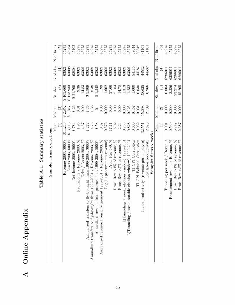
AO

nline

App

endix

Table

A.1

:Sum

mary

stati

stic

s

Sam

ple

:fi

rms

xele

cti

on

s Mea

nM

edia

nS

t.d

ev.

Nof

ob

sN

of

firm

s(1

)(2

)(3

)(4

)(5

)R

even

ue

2003,

$000’s

$14,2

46

$2,8

52

$105,6

60

63021

45275

Ass

ets

2003,

$000’s

$13,1

13

$1,3

17

$173,9

33

63008

45264

Net

Inco

me

2003,

$000’s

$784

$26

$21,7

60

62804

45102

Net

Inco

me

/R

even

ue

2003,

%1.9

50.8

19.3

863021

45275

Deb

t/

Ass

ets

2003,

%4.3

70.0

014.8

363021

45275

An

nu

aliz

edtr

ansf

ers

tofl

y-b

y-n

ight

firm

s1999-2

004,

$000’s

$272

$36

$5,9

09

63021

45275

An

nu

aliz

edtr

ansf

ers

tofl

y-b

y-n

ight

firm

s1999-2

004

/R

even

ue

2003,

%4.7

51.3

68.3

863021

45275

An

nu

aliz

edre

ven

ue

from

pro

cure

men

t1999-2

004,

$000’s

$58

$-

$1,5

48

63021

45275

An

nu

aliz

edre

ven

ue

from

pro

cure

men

t1999-2

004

/R

even

ue

2003,

%0.3

70.0

01.9

963021

45275

Log(1

+p

rocu

rem

ent

reven

ue)

0.5

72

0.0

00

1.6

02

63021

45275

Pro

c.R

ev>

0,

%17.1

10.0

037.6

663021

45275

Pro

c.R

ev>

1%

of

reve

nu

e,%

5.0

20.0

021.8

463021

45275

Pro

c.R

ev>

5%

of

reve

nu

e,%

2.2

40.0

014.7

863021

45275

L(T

un

nel

ing

/w

eek,

elec

tion

win

dow

),1999-2

004

0.7

58

0.0

00

1.3

13

63021

45275

L(T

un

nel

ing

/w

eek,

outs

ide

elec

tion

win

dow

),1999-2

004

0.8

28

0.1

25

1.2

32

63021

45275

TI

CP

IC

orr

up

tion

0.0

00

0.4

57

1.0

00

54115

38044

TI

CP

IP

oli

tica

lC

orr

up

tion

0.0

32

0.0

31

0.0

30

44787

30842

Lab

orp

rod

uct

ivit

y(r

even

ue

per

emp

loyee

)32.5

51

15.0

08

58.6

25

44532

31101

Log

lab

or

pro

du

ctiv

ity

2.8

73

2.7

09

0.9

66

44532

31101

Sam

ple

:fi

rms

xw

eeks M

ean

Med

ian

St.

dev

.N

of

ob

sN

of

firm

s(1

)(2

)(3

)(4

)(5

)T

un

nel

ing

per

wee

k/

Rev

enu

e0.0

01

0.0

00

0.0

03

6286011

45275

Pro

cure

men

tre

ven

ue

/R

even

ue,

%0.5

30

0.0

00

3.3

86

6286011

45275

Pro

c.R

ev>

1%

of

reve

nu

e,%

5.7

47

0.0

00

23.2

74

6286011

45275

Pro

c.R

ev>

5%

of

reve

nu

e,%

2.3

87

0.0

00

15.2

65

6286011

45275

45

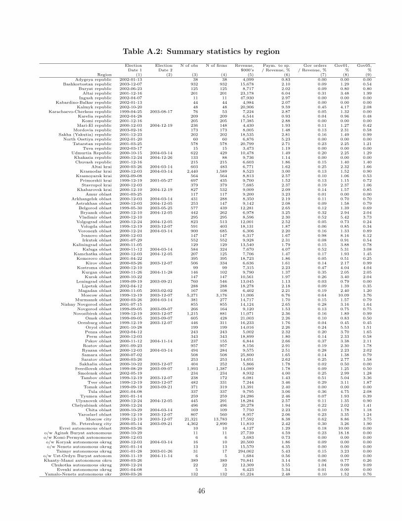
Table A.2: Summary statistics by region

Election Election N of obs N of firms Revenue, Paym. to sp. Gov orders Gov01, Gov05,Date 1 Date 2 $000’s / Revenue, % / Revenue, % % %

Region (1) (2) (3) (4) (5) (6) (7) (8) (9)Adygeya republic 2002-01-13 38 38 4,099 0.83 0.00 0.00 0.00

Bashkortostan republic 2003-12-07 932 932 15,678 2.10 0.09 1.29 0.54Buryat republic 2002-06-23 125 125 8,717 2.02 0.09 0.80 0.80

Altai republic 2001-12-16 201 201 23,178 6.04 0.31 3.48 1.99Ingush republic 2002-04-07 11 11 47,930 2.97 0.00 0.00 0.00

Kabardino-Balkar republic 2002-01-13 44 44 4,984 2.07 0.00 0.00 0.00Kalmyk republic 2002-10-20 48 48 20,906 9.59 0.45 4.17 2.08

Karachaevo-Cherkess republic 1999-04-25 2003-08-17 76 53 7,224 2.87 0.05 1.32 0.00Karelia republic 2002-04-28 209 209 6,544 0.93 0.04 0.96 0.48

Komi republic 2001-12-16 205 205 17,385 2.88 0.00 0.00 0.00Mari-El republic 2000-12-03 2004-12-19 236 148 4,430 1.93 0.11 1.27 0.42

Mordovia republic 2003-02-16 173 173 8,005 1.48 0.13 2.31 0.58Sakha (Yakutia) republic 2001-12-23 202 202 18,535 2.81 0.16 1.49 0.99

North Osetiya republic 2002-01-20 60 60 6,876 5.23 0.00 0.00 0.00Tatarstan republic 2001-03-25 578 578 20,799 2.71 0.23 2.25 1.21

Tuva republic 2002-03-17 15 15 3,473 1.19 0.00 0.00 0.00Udmurtia Republic 2000-10-15 2004-03-14 622 429 10,478 1.49 0.20 2.25 1.29Khakasia republic 2000-12-24 2004-12-26 133 88 9,736 1.14 0.00 0.00 0.00Chuvash republic 2001-12-16 215 215 6,603 1.86 0.15 1.40 1.40

Altai krai 2000-03-26 2004-03-14 603 483 6,771 1.62 0.25 2.32 1.66Krasnodar krai 2000-12-03 2004-03-14 2,440 1,589 8,523 3.00 0.13 1.52 0.90

Krasnoyarsk krai 2002-09-08 564 564 8,813 2.57 0.10 1.06 0.53Primorskii krai 1999-12-19 2001-05-27 697 435 9,700 1.52 0.13 1.15 0.72Stavropol krai 2000-12-03 379 379 7,685 2.37 0.19 2.37 1.06

Khabarovsk krai 2000-12-10 2004-12-19 827 532 9,009 2.09 0.14 1.57 0.85Amur oblast 2001-03-25 117 117 9,200 3.23 0.01 0.00 0.00

Arkhangelsk oblast 2000-12-03 2004-03-14 431 288 8,350 2.19 0.11 0.70 0.70Astrakhan oblast 2000-12-03 2004-12-05 253 147 9,142 2.08 0.09 1.58 0.79

Belgorod oblast 1999-05-30 2003-05-25 577 439 12,281 2.65 0.12 1.39 0.69Bryansk oblast 2000-12-10 2004-12-05 442 262 6,978 3.25 0.32 2.94 2.04

Vladimir oblast 2000-12-10 295 295 8,596 2.30 0.52 5.42 3.73Volgograd oblast 2000-12-24 2004-12-05 823 513 12,001 2.52 0.05 0.73 0.24

Vologda oblast 1999-12-19 2003-12-07 591 403 18,131 1.87 0.06 0.85 0.34Voronezh oblast 2000-12-24 2004-03-14 900 685 6,306 2.20 0.16 1.33 0.89

Ivanovo oblast 2000-12-03 147 147 6,317 1.67 0.98 8.16 6.12Irkutsk oblast 2001-07-29 552 552 9,928 2.31 0.08 0.91 0.54

Kaliningrad oblast 2000-11-05 129 129 13,540 1.79 0.15 3.88 0.78Kaluga oblast 2000-11-12 2004-03-14 584 324 7,670 4.07 0.52 5.31 3.08

Kamchatka oblast 2000-12-03 2004-12-05 207 125 7,706 1.47 0.17 1.93 1.45Kemerovo oblast 2001-04-22 395 395 18,723 1.86 0.05 0.51 0.25

Kirov oblast 2000-03-26 2003-12-07 506 334 6,636 1.61 0.14 2.17 0.99Kostroma oblast 2000-12-10 99 99 7,315 2.23 0.47 4.04 4.04

Kurgan oblast 2000-11-26 2004-11-28 146 102 9,790 1.37 0.35 2.05 2.05Kursk oblast 2000-10-22 147 147 10,561 1.97 0.26 3.40 2.04

Leningrad oblast 1999-09-19 2003-09-21 760 546 13,045 1.13 0.03 0.79 0.00Lipetsk oblast 2002-04-12 288 288 18,278 2.18 0.09 1.39 0.35

Magadan oblast 2000-11-05 2003-02-02 167 108 6,402 2.21 0.19 2.40 1.20Moscow oblast 1999-12-19 2003-12-07 5,271 3,176 11,006 6.76 0.64 10.09 3.76

Murmansk oblast 2000-03-26 2004-03-14 381 277 14,717 1.70 0.15 1.57 0.79Nizhny Novgorod oblast 2001-07-15 855 855 14,124 2.65 0.28 3.16 1.64

Novgorod oblast 1999-09-05 2003-09-07 266 164 9,120 1.53 0.13 0.75 0.75Novosibirsk oblast 1999-12-19 2003-12-07 1,215 881 11,071 2.36 0.16 1.89 0.99

Omsk oblast 1999-09-05 2003-09-07 605 428 21,003 2.26 0.10 0.83 0.50Orenburg oblast 1999-12-19 2003-12-07 446 311 16,233 1.76 0.04 0.45 0.45

Oryol oblast 2001-10-28 199 199 14,016 2.26 0.24 5.53 1.51Penza oblast 2002-04-12 243 243 5,002 2.32 0.20 3.70 1.65Perm oblast 2000-12-03 343 343 18,899 1.80 0.14 2.33 0.58Pskov oblast 2000-11-12 2004-11-14 237 155 6,844 2.66 0.37 3.38 2.11

Rostov oblast 2001-09-23 957 957 8,156 2.91 0.19 2.30 1.78Ryazan oblast 2000-12-03 2004-03-14 494 284 9,575 2.51 0.28 2.23 2.02Samara oblast 2000-07-02 508 508 25,800 1.65 0.14 1.38 0.79Saratov oblast 2000-03-26 253 253 14,651 2.62 0.25 2.77 1.58

Sakhalin oblast 2000-10-22 2003-12-07 404 252 5,866 1.78 0.02 0.50 0.00Sverdlovsk oblast 1999-08-29 2003-09-07 1,993 1,387 14,089 1.78 0.09 1.25 0.50

Smolensk oblast 2002-05-19 234 234 8,932 4.00 0.25 2.99 1.28Tambov oblast 1999-12-19 2003-12-07 238 172 6,081 1.43 0.51 5.04 3.36

Tver oblast 1999-12-19 2003-12-07 482 331 7,244 3.46 0.29 3.11 1.87Tomsk oblast 1999-09-19 2003-09-21 371 319 13,391 2.40 0.00 0.00 0.00

Tula oblast 2001-04-08 337 337 9,795 3.06 0.36 4.75 2.08Tyumen oblast 2001-01-14 259 259 24,286 2.46 0.07 1.93 0.39

Ulyanovsk oblast 2000-12-24 2004-12-05 445 291 18,284 2.57 0.11 1.35 0.90Chelyabinsk oblast 2000-12-24 496 496 20,278 1.94 0.22 2.02 1.41

Chita oblast 2000-10-29 2004-03-14 169 109 7,750 2.23 0.10 1.78 1.18Yaroslavl oblast 1999-12-19 2003-12-07 807 560 8,957 2.06 0.23 3.35 1.24

Moscow city 1999-12-19 2003-12-07 21,321 13,783 17,592 8.38 0.62 8.86 3.75St. Petersburg city 2000-05-14 2003-09-21 4,362 2,890 11,810 2.42 0.30 3.26 1.90

Evrei autonomous oblast 2000-03-26 10 10 4,127 1.29 0.18 10.00 0.00o/w Aginsk Buryat autonomous 2000-10-29 11 11 27,739 4.59 0.23 18.18 0.00o/w Komi-Permyak autonomous 2000-12-03 6 6 3,683 0.73 0.00 0.00 0.00o/w Koryak autonomous okrug 2000-12-03 2004-03-14 16 10 20,500 1.86 0.09 0.00 0.00o/w Nenets autonomous okrug 2001-01-14 13 13 15,570 4.35 0.00 0.00 0.00

Taimyr autonomous okrug 2001-01-28 2003-01-26 31 17 294,062 5.43 0.15 3.23 0.00o/w Ust-Ordyn Buryat autonom 2000-11-19 2004-11-14 6 5 1,684 0.56 0.00 0.00 0.00Khanty-Mansi autonomous okru 2000-03-26 389 389 70,841 3.14 0.06 0.77 0.26

Chukotka autonomous okrug 2000-12-24 22 22 12,309 3.55 1.04 9.09 9.09Evenki autonomous okrug 2001-04-08 5 5 6,423 5.34 0.01 0.00 0.00

Yamalo-Nenets autonomous okr 2000-03-26 132 132 61,224 2.48 0.10 1.52 0.76

46

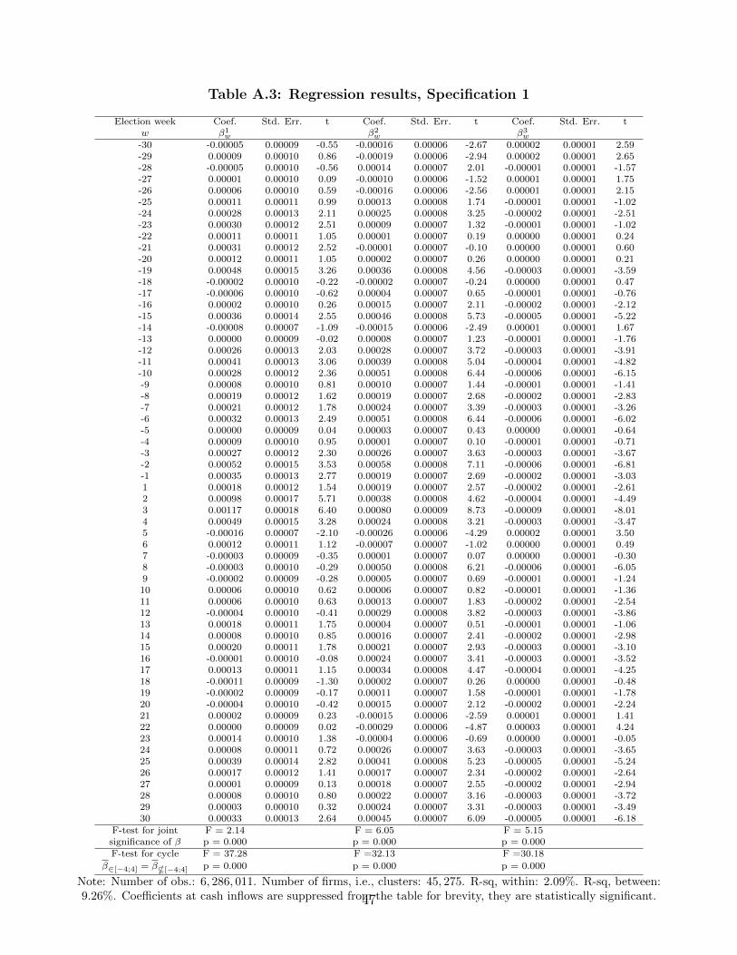
Table A.3: Regression results, Specification 1

Election week Coef. Std. Err. t Coef. Std. Err. t Coef. Std. Err. tw β1

w β2w β3

w

-30 -0.00005 0.00009 -0.55 -0.00016 0.00006 -2.67 0.00002 0.00001 2.59-29 0.00009 0.00010 0.86 -0.00019 0.00006 -2.94 0.00002 0.00001 2.65-28 -0.00005 0.00010 -0.56 0.00014 0.00007 2.01 -0.00001 0.00001 -1.57-27 0.00001 0.00010 0.09 -0.00010 0.00006 -1.52 0.00001 0.00001 1.75-26 0.00006 0.00010 0.59 -0.00016 0.00006 -2.56 0.00001 0.00001 2.15-25 0.00011 0.00011 0.99 0.00013 0.00008 1.74 -0.00001 0.00001 -1.02-24 0.00028 0.00013 2.11 0.00025 0.00008 3.25 -0.00002 0.00001 -2.51-23 0.00030 0.00012 2.51 0.00009 0.00007 1.32 -0.00001 0.00001 -1.02-22 0.00011 0.00011 1.05 0.00001 0.00007 0.19 0.00000 0.00001 0.24-21 0.00031 0.00012 2.52 -0.00001 0.00007 -0.10 0.00000 0.00001 0.60-20 0.00012 0.00011 1.05 0.00002 0.00007 0.26 0.00000 0.00001 0.21-19 0.00048 0.00015 3.26 0.00036 0.00008 4.56 -0.00003 0.00001 -3.59-18 -0.00002 0.00010 -0.22 -0.00002 0.00007 -0.24 0.00000 0.00001 0.47-17 -0.00006 0.00010 -0.62 0.00004 0.00007 0.65 -0.00001 0.00001 -0.76-16 0.00002 0.00010 0.26 0.00015 0.00007 2.11 -0.00002 0.00001 -2.12-15 0.00036 0.00014 2.55 0.00046 0.00008 5.73 -0.00005 0.00001 -5.22-14 -0.00008 0.00007 -1.09 -0.00015 0.00006 -2.49 0.00001 0.00001 1.67-13 0.00000 0.00009 -0.02 0.00008 0.00007 1.23 -0.00001 0.00001 -1.76-12 0.00026 0.00013 2.03 0.00028 0.00007 3.72 -0.00003 0.00001 -3.91-11 0.00041 0.00013 3.06 0.00039 0.00008 5.04 -0.00004 0.00001 -4.82-10 0.00028 0.00012 2.36 0.00051 0.00008 6.44 -0.00006 0.00001 -6.15-9 0.00008 0.00010 0.81 0.00010 0.00007 1.44 -0.00001 0.00001 -1.41-8 0.00019 0.00012 1.62 0.00019 0.00007 2.68 -0.00002 0.00001 -2.83-7 0.00021 0.00012 1.78 0.00024 0.00007 3.39 -0.00003 0.00001 -3.26-6 0.00032 0.00013 2.49 0.00051 0.00008 6.44 -0.00006 0.00001 -6.02-5 0.00000 0.00009 0.04 0.00003 0.00007 0.43 0.00000 0.00001 -0.64-4 0.00009 0.00010 0.95 0.00001 0.00007 0.10 -0.00001 0.00001 -0.71-3 0.00027 0.00012 2.30 0.00026 0.00007 3.63 -0.00003 0.00001 -3.67-2 0.00052 0.00015 3.53 0.00058 0.00008 7.11 -0.00006 0.00001 -6.81-1 0.00035 0.00013 2.77 0.00019 0.00007 2.69 -0.00002 0.00001 -3.031 0.00018 0.00012 1.54 0.00019 0.00007 2.57 -0.00002 0.00001 -2.612 0.00098 0.00017 5.71 0.00038 0.00008 4.62 -0.00004 0.00001 -4.493 0.00117 0.00018 6.40 0.00080 0.00009 8.73 -0.00009 0.00001 -8.014 0.00049 0.00015 3.28 0.00024 0.00008 3.21 -0.00003 0.00001 -3.475 -0.00016 0.00007 -2.10 -0.00026 0.00006 -4.29 0.00002 0.00001 3.506 0.00012 0.00011 1.12 -0.00007 0.00007 -1.02 0.00000 0.00001 0.497 -0.00003 0.00009 -0.35 0.00001 0.00007 0.07 0.00000 0.00001 -0.308 -0.00003 0.00010 -0.29 0.00050 0.00008 6.21 -0.00006 0.00001 -6.059 -0.00002 0.00009 -0.28 0.00005 0.00007 0.69 -0.00001 0.00001 -1.2410 0.00006 0.00010 0.62 0.00006 0.00007 0.82 -0.00001 0.00001 -1.3611 0.00006 0.00010 0.63 0.00013 0.00007 1.83 -0.00002 0.00001 -2.5412 -0.00004 0.00010 -0.41 0.00029 0.00008 3.82 -0.00003 0.00001 -3.8613 0.00018 0.00011 1.75 0.00004 0.00007 0.51 -0.00001 0.00001 -1.0614 0.00008 0.00010 0.85 0.00016 0.00007 2.41 -0.00002 0.00001 -2.9815 0.00020 0.00011 1.78 0.00021 0.00007 2.93 -0.00003 0.00001 -3.1016 -0.00001 0.00010 -0.08 0.00024 0.00007 3.41 -0.00003 0.00001 -3.5217 0.00013 0.00011 1.15 0.00034 0.00008 4.47 -0.00004 0.00001 -4.2518 -0.00011 0.00009 -1.30 0.00002 0.00007 0.26 0.00000 0.00001 -0.4819 -0.00002 0.00009 -0.17 0.00011 0.00007 1.58 -0.00001 0.00001 -1.7820 -0.00004 0.00010 -0.42 0.00015 0.00007 2.12 -0.00002 0.00001 -2.2421 0.00002 0.00009 0.23 -0.00015 0.00006 -2.59 0.00001 0.00001 1.4122 0.00000 0.00009 0.02 -0.00029 0.00006 -4.87 0.00003 0.00001 4.2423 0.00014 0.00010 1.38 -0.00004 0.00006 -0.69 0.00000 0.00001 -0.0524 0.00008 0.00011 0.72 0.00026 0.00007 3.63 -0.00003 0.00001 -3.6525 0.00039 0.00014 2.82 0.00041 0.00008 5.23 -0.00005 0.00001 -5.2426 0.00017 0.00012 1.41 0.00017 0.00007 2.34 -0.00002 0.00001 -2.6427 0.00001 0.00009 0.13 0.00018 0.00007 2.55 -0.00002 0.00001 -2.9428 0.00008 0.00010 0.80 0.00022 0.00007 3.16 -0.00003 0.00001 -3.7229 0.00003 0.00010 0.32 0.00024 0.00007 3.31 -0.00003 0.00001 -3.4930 0.00033 0.00013 2.64 0.00045 0.00007 6.09 -0.00005 0.00001 -6.18

F-test for joint F = 2.14 F = 6.05 F = 5.15significance of β p = 0.000 p = 0.000 p = 0.000F-test for cycle F = 37.28 F =32.13 F =30.18

β∈[−4;4] = β*[−4;4] p = 0.000 p = 0.000 p = 0.000

Note: Number of obs.: 6, 286, 011. Number of firms, i.e., clusters: 45, 275. R-sq, within: 2.09%. R-sq, between:9.26%. Coefficients at cash inflows are suppressed from the table for brevity, they are statistically significant.47

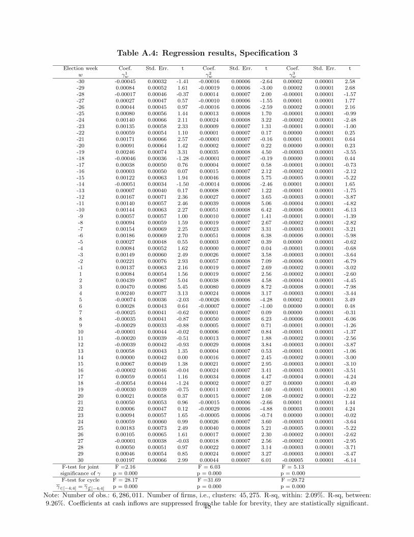
Table A.4: Regression results, Specification 3

Election week Coef. Std. Err. t Coef. Std. Err. t Coef. Std. Err. tw γ1

w γ2w γ3

w

-30 -0.00045 0.00032 -1.41 -0.00016 0.00006 -2.64 0.00002 0.00001 2.58-29 0.00084 0.00052 1.61 -0.00019 0.00006 -3.00 0.00002 0.00001 2.68-28 -0.00017 0.00046 -0.37 0.00014 0.00007 2.00 -0.00001 0.00001 -1.57-27 0.00027 0.00047 0.57 -0.00010 0.00006 -1.55 0.00001 0.00001 1.77-26 0.00044 0.00045 0.97 -0.00016 0.00006 -2.59 0.00002 0.00001 2.16-25 0.00080 0.00056 1.44 0.00013 0.00008 1.70 -0.00001 0.00001 -0.99-24 0.00140 0.00066 2.11 0.00024 0.00008 3.22 -0.00002 0.00001 -2.48-23 0.00135 0.00058 2.33 0.00009 0.00007 1.31 -0.00001 0.00001 -1.00-22 0.00059 0.00054 1.10 0.00001 0.00007 0.17 0.00000 0.00001 0.25-21 0.00171 0.00066 2.57 -0.00001 0.00007 -0.16 0.00001 0.00001 0.64-20 0.00091 0.00064 1.42 0.00002 0.00007 0.22 0.00000 0.00001 0.23-19 0.00246 0.00074 3.31 0.00035 0.00008 4.50 -0.00003 0.00001 -3.55-18 -0.00046 0.00036 -1.28 -0.00001 0.00007 -0.19 0.00000 0.00001 0.44-17 0.00038 0.00050 0.76 0.00004 0.00007 0.58 -0.00001 0.00001 -0.73-16 0.00003 0.00050 0.07 0.00015 0.00007 2.12 -0.00002 0.00001 -2.12-15 0.00122 0.00063 1.94 0.00046 0.00008 5.75 -0.00005 0.00001 -5.22-14 -0.00051 0.00034 -1.50 -0.00014 0.00006 -2.46 0.00001 0.00001 1.65-13 0.00007 0.00040 0.17 0.00008 0.00007 1.22 -0.00001 0.00001 -1.75-12 0.00167 0.00071 2.36 0.00027 0.00007 3.65 -0.00003 0.00001 -3.87-11 0.00140 0.00057 2.46 0.00039 0.00008 5.06 -0.00004 0.00001 -4.82-10 0.00144 0.00063 2.27 0.00051 0.00008 6.42 -0.00006 0.00001 -6.13-9 0.00057 0.00057 1.00 0.00010 0.00007 1.41 -0.00001 0.00001 -1.39-8 0.00094 0.00059 1.59 0.00019 0.00007 2.67 -0.00002 0.00001 -2.82-7 0.00154 0.00069 2.25 0.00023 0.00007 3.31 -0.00003 0.00001 -3.21-6 0.00186 0.00069 2.70 0.00051 0.00008 6.38 -0.00006 0.00001 -5.98-5 0.00027 0.00048 0.55 0.00003 0.00007 0.39 0.00000 0.00001 -0.62-4 0.00084 0.00052 1.62 0.00000 0.00007 0.04 -0.00001 0.00001 -0.68-3 0.00149 0.00060 2.49 0.00026 0.00007 3.58 -0.00003 0.00001 -3.64-2 0.00221 0.00076 2.93 0.00057 0.00008 7.09 -0.00006 0.00001 -6.79-1 0.00137 0.00063 2.16 0.00019 0.00007 2.69 -0.00002 0.00001 -3.021 0.00084 0.00054 1.56 0.00019 0.00007 2.56 -0.00002 0.00001 -2.602 0.00439 0.00087 5.04 0.00038 0.00008 4.58 -0.00004 0.00001 -4.453 0.00470 0.00086 5.45 0.00080 0.00009 8.72 -0.00008 0.00001 -7.984 0.00240 0.00077 3.13 0.00024 0.00008 3.17 -0.00003 0.00001 -3.445 -0.00074 0.00036 -2.03 -0.00026 0.00006 -4.28 0.00002 0.00001 3.496 0.00028 0.00043 0.64 -0.00007 0.00007 -1.00 0.00000 0.00001 0.487 -0.00025 0.00041 -0.62 0.00001 0.00007 0.09 0.00000 0.00001 -0.318 -0.00035 0.00041 -0.87 0.00050 0.00008 6.23 -0.00006 0.00001 -6.069 -0.00029 0.00033 -0.88 0.00005 0.00007 0.71 -0.00001 0.00001 -1.2610 -0.00001 0.00044 -0.02 0.00006 0.00007 0.84 -0.00001 0.00001 -1.3711 -0.00020 0.00039 -0.51 0.00013 0.00007 1.88 -0.00002 0.00001 -2.5612 -0.00039 0.00042 -0.93 0.00029 0.00008 3.84 -0.00003 0.00001 -3.8713 0.00058 0.00043 1.35 0.00004 0.00007 0.53 -0.00001 0.00001 -1.0614 0.00000 0.00042 0.00 0.00016 0.00007 2.45 -0.00002 0.00001 -3.0015 0.00067 0.00049 1.38 0.00021 0.00007 2.95 -0.00003 0.00001 -3.1016 -0.00002 0.00046 -0.04 0.00024 0.00007 3.41 -0.00003 0.00001 -3.5117 0.00059 0.00051 1.16 0.00034 0.00008 4.47 -0.00004 0.00001 -4.2418 -0.00054 0.00044 -1.24 0.00002 0.00007 0.27 0.00000 0.00001 -0.4919 -0.00030 0.00039 -0.75 0.00011 0.00007 1.60 -0.00001 0.00001 -1.8020 0.00021 0.00058 0.37 0.00015 0.00007 2.08 -0.00002 0.00001 -2.2221 0.00050 0.00053 0.96 -0.00015 0.00006 -2.66 0.00001 0.00001 1.4422 0.00006 0.00047 0.12 -0.00029 0.00006 -4.88 0.00003 0.00001 4.2423 0.00094 0.00057 1.65 -0.00005 0.00006 -0.74 0.00000 0.00001 -0.0224 0.00059 0.00060 0.99 0.00026 0.00007 3.60 -0.00003 0.00001 -3.6425 0.00183 0.00073 2.49 0.00040 0.00008 5.21 -0.00005 0.00001 -5.2226 0.00105 0.00065 1.61 0.00017 0.00007 2.30 -0.00002 0.00001 -2.6227 -0.00001 0.00038 -0.03 0.00018 0.00007 2.56 -0.00002 0.00001 -2.9528 0.00050 0.00051 0.97 0.00022 0.00007 3.14 -0.00003 0.00001 -3.7129 0.00046 0.00054 0.85 0.00024 0.00007 3.27 -0.00003 0.00001 -3.4730 0.00197 0.00066 2.99 0.00044 0.00007 6.01 -0.00005 0.00001 -6.14

F-test for joint F =2.16 F = 6.03 F = 5.13significance of γ p = 0.000 p = 0.000 p = 0.000F-test for cycle F = 28.17 F =31.69 F =29.72

γ∈[−4;4] = γ*[−4;4] p = 0.000 p = 0.000 p = 0.000

Note: Number of obs.: 6, 286, 011. Number of firms, i.e., clusters: 45, 275. R-sq, within: 2.09%. R-sq, between:9.26%. Coefficients at cash inflows are suppressed from the table for brevity, they are statistically significant.48

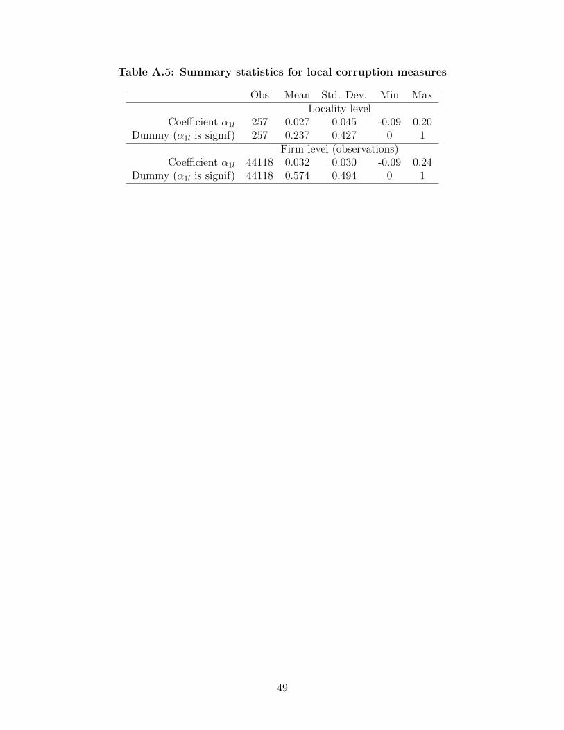
Table A.5: Summary statistics for local corruption measures

Obs Mean Std. Dev. Min MaxLocality level

Coefficient α1l 257 0.027 0.045 -0.09 0.20Dummy (α1l is signif) 257 0.237 0.427 0 1

Firm level (observations)Coefficient α1l 44118 0.032 0.030 -0.09 0.24

Dummy (α1l is signif) 44118 0.574 0.494 0 1

49

B Data Appendix

B.1 Data Sources Used in Addition to Banking Transactions Data

In addition to the list of banking transactions, we use two other data sources. The first source isthe Rosstat (Russia’s official statistical agency) database of Russian companies provided by Spark(http://www.ispark.ru/en-US/default.aspx). This database contains a firm’s INN, name, region,date of registration, industry, directors, owners, and other identifying information about the firm.In addition, it contains basic accounting data, such as revenue, profit, net income, assets, anddebt. According to Russian law, all firms (even small ones) must report their balance sheets andincome statements to Rosstat on a quarterly basis. Although this law does not set any explicitpenalty for firms that do not report, the majority of Russian firms report their data to Rosstatto maintain good relations with the tax authorities. Rosstat contains accounting data for about1.5 million Russian firms.

The second dataset includes the personal income of Moscow residents. It contains more than 7million records for 2002, and more than 9 million records for 2003 and 2004. Each entry containsunique identification data (name, address, identification number) for both employer and employee.There can be multiple records per person if a person receives income from several sources. Gurievand Rachinsky (2006) use these data to measure income inequality in the presence of super-richindividuals. We use this dataset to get the number of tax agency employees.

B.2 Description of Variables Used in the Analysis

B.2.1 Sample: firms x elections

• Revenue, 2003 - Company’s book revenue in 2003 taken from Rosstat

• Assets, 2003 - Company’s book assets in 2003 taken from Rosstat

• Net Income, 2003 - Company’s net income in 2003 taken from Rosstat

• Debt, 2003 - A sum of company’s short term debt in 2003 and long term debt in 2003,which are taken from Rosstat

• Annualized transfers to fly-by-night firms 1999-2004 - Total transfers to fly-by-night firmsby a firm in 1999-2004 divided by six. The transfers to fly-by-night firms are calculatedusing the banking transaction database. See Mironov (2013) for a detailed description ofthe identification procedure of fly-by-night firms. These firms are referred to as “spacemen”in Mironov (2013).

• Annualized revenue from procurement, 1 year after election - Total transfers from government-affiliated entities to a firm, which have the reported purpose of payment for goods andservices during one year after the election. These transfers are calculated using the bank-ing transaction database. In the baseline analysis, we exclude payments for utilities, e.g.,electricity and water, from the list of revenues from public procurement contracts becausethese contracts are not usually allocated on a competitive basis and are automatically al-located to local monopolists. (None of the results changes if we keep utilities in definition

50

of public procurement.) If the election date happened to be in 2004, then we divide thetotal transfers by the number of days left until the end of 2004 and multiply by 365 (to getannualized revenue from procurement).

• Tunneling per week, election window - We calculate total transfers to fly-by-night firms bya firm from 4 weeks before until 4 weeks after the election and divide by 8. If the electionperiod overlapped with our sample period and is shorter than 8 weeks, then we dividethe transfers to fly-by-night firms by the actual number of weeks presented in our sampleperiod (1999-2004). For example, if the date of the election is 2004-12-19, then we dividethe transfers to fly-by-night firms by 5.7.

• Tunneling per week, outside election window - We calculate total transfers to fly-by-nightfirms by a firm starting one year before the election date and ending 4 weeks before theelection. Then, we divide this number by the actual number of weeks presented in oursample period.

• Perceived corruption - see section 4.2 of the paper for description

• Tax-agency-level corruption - see section 5 of the paper for description

• Number of employees - number of firm’s employees in 2003 taken from Rosstat

B.2.2 Sample: Firms x Weeks

• Tunneling per week - Transfers to fly-by-night firms during a specific week.

• Tunneling per year - Annualized transfer to fly-by-night firms from one year before untilone year after the election. For example, if the election date is 2004-03-14 then we taketotal transfers to fly-by-night firms from 2003-03-14 to 2004-12-31. After that we divide thisnumber by the number of days in the period from 2003-03-14 to 2004-12-31 and multiplyby 365. If the election date is 2003-12-07 then we take total transfers to fly-by-night firmsfrom 2002-12-07 to 2004-12-07 and divide them by 2.

• Revenue - Company’s book revenue in 2003 taken from Rosstat

• Procurement revenue - Annualized transfers from government-affiliated entities from oneyear before until one year after the election. We include only transactions that have thereported purpose of payment for goods and services. We exclude payments for utilities, e.g.,electricity and water, from the list of revenues from public procurement contracts.

51