cost-conscious manufacturing – models and methods · pdf filecost-conscious...

LUND UNIVERSITY

PO Box 117221 00 Lund+46 46-222 00 00

Cost-conscious manufacturing – Models and methods for analyzing present and futureperformance from a cost perspective

Jönsson, Mathias

Published: 2012-01-01

Link to publication

Citation for published version (APA):Jönsson, M. (2012). Cost-conscious manufacturing – Models and methods for analyzing present and futureperformance from a cost perspective

General rightsCopyright and moral rights for the publications made accessible in the public portal are retained by the authorsand/or other copyright owners and it is a condition of accessing publications that users recognise and abide by thelegal requirements associated with these rights.

• Users may download and print one copy of any publication from the public portal for the purpose of privatestudy or research. • You may not further distribute the material or use it for any profit-making activity or commercial gain • You may freely distribute the URL identifying the publication in the public portal

http://portal.research.lu.se/portal/en/publications/costconscious-manufacturing--models-and-methods-for-analyzing-present-and-future-performance-from-a-cost-perspective(030ee6a6-0edb-490c-afbd-2fe7f681e330).html

Cost-conscious manufacturing – Models and methods for analyzing present and future

performance from a cost perspective

Mathias Jönsson

Division of Production and Materials Engineering, Lund University

Division of Production and Materials Engineering, Lund University Box 118, SE-221 00 Lund, Sweden ISBN 978-91-7473-277-1 LUTMDN(TMMV-1063)/1-85(2012) © Mathias Jönsson, and Division of Production and Materials Engineering, Lund University, 2012 Printed by Media-Tryck, Lund, Sweden, 2012

I

Abstract Manufacturing is an industry in which the effects of globalization are obvious. Manufacturing costs are a key factor in this respect and affect, for example, decisions about offshoring, i.e., moving production abroad. If Sweden and other Western countries are to maintain large manufacturing sectors, they must be competitive, making cost one of the most critical parameters.

The work presented here seeks to develop tools for cost-conscious manufacturing. These tools should provide insight into how well a manufacturing system is performing and support the analysis and prioritization of manufacturing development activities. To achieve this objective, two research questions were formulated.

The first research question (RQ1) concerns how a general cost model should be designed to take into consideration the most important process-near parameters influencing manufacturing system performance. A cost model developed in accordance with this research question includes critical parameters affecting performance, such as cycle time, setup time, and performance loss parameters. The model is centered on the processing steps involved in processing a part. The losses occurring in the processing steps are important in the model, so the links between structured, detailed monitoring of the loss causes and their impacts on costs are emphasized. Modified versions of the model to analyze volume flexibility and downtime variability are also presented.

The second research question (RQ2) concerns how such a cost model can be used in practice, i.e., the requirements and conditions for industrial use. Implementation in an automotive company indicated that the model was applicable in this context and that interesting insights into manufacturing costs could be gained from using the model. A study of the industrial conditions for applying the cost model identified software products for collecting manufacturing loss data that support the level of detail needed for model input, but found that manufacturing companies do not necessarily collect such detailed data. A demonstration program developed based on the databases available in a collaborating company indicated how the cost model could be used practically in a company. The somewhat deficient detail in the collected loss data, found in the above study, led to an inquiry in another company into the pros and cons of collecting highly detailed performance loss data. The results identified more advantages than disadvantages with collecting more detailed data: the operators responsible for data collection did not perceive any particular difficulties with the increased detail and the production manager believed that the increased detail led to better knowledge of performance losses.

Keywords: manufacturing cost, cost models, performance analysis

II

Sammanfattning Tillverkningsindustrin är en bransch där globaliseringen är högst påtaglig. Konkurrensen är global, vilket medför att exempelvis produktionsanläggningar i Sverige konkurrerar med anläggningar i länder med betydligt lägre lönenivå. Om Sverige även i fortsättningen ska ha en konkurrenskraftig tillverkningsindustri krävs att produktionen bedrivs med en hög kostnadsmedvetenhet. Med det åsyftas att produktionspersonalen har kunskap om hur olika parametrar i ett tillverkningssystem påverkar kostnaden för de produkter som produceras samt hur tillverkningskostnaden är fördelad mellan olika kostnadsposter. Med den kunskapen kan produktionsutvecklingsarbete bedrivas med en högre medvetenhet om hur olika utvecklingsinsatser påverkar tillverkningskostnaden och därmed med bättre precision kunna prioritera vilka utvecklingsinsatser som bör genomföras för att bli mer kostnadseffektiv.

Syftet med forskningen som presenteras här är att utveckla ett koncept bestående av modeller och metoder för att skapa kostnadsmedveten produktion. Konceptet ska ge insikter om hur väl ett tillverkningssystem fungerar och utgöra ett stöd vid analyser och prioriteringar gällande utvecklingsinsatser av tillverkningssystemet. För att nå syftet har två forskningsfrågor formulerats.

Den första forskningsfrågan behandlar hur en generell kostnadsmodell bör utformas som beaktar de viktigaste parametrarna som beskriver ett tillverkningssystems prestanda. En kostnadsmodell som beskriver kostnaden per tillverkad detalj har utvecklats i enlighet med den frågeställningen. I modellen ingår kritiska parametrar som påverkar tillverkningssystemets prestanda, såsom cykeltid, ställtid, kassationer och stillestånd. De förluster som uppkommer vid varje förädlingssteg är centrala för modellen. En annan viktig aspekt är att uppföljningen av orsakerna till förlusterna bör vara både strukturerad och detaljerad för att därmed kunna beräkna varje orsaks inverkan på tillverkningskostnaden. Kostnadsmodellen kan anses utgöra en länk mellan tekniska och ekonomiska parametrar i ett tillverkningssystem och kan därmed användas för att analysera kopplingen mellan dessa.

Den andra forskningsfrågan behandlar förutsättningarna för att en sådan kostnadsmodell ska kunna användas i praktiken, det vill säga dess industriella tillämpbarhet. För att besvara den frågan gjordes först en implementering av modellen på ett företag inom fordonsindustrin, som visade att modellen var tillämpbar i detta fall och att detaljerade analyser av tillverkningskostnaderna kunde göras med hjälp av modellen. En annan studie visade att det finns programvaror på marknaden för produktionsuppföljning som stödjer insamling av all den indata som behövs till kostnadsmodellen gällande produktionsstörningar och dess orsaker, men att tillverkande företag nödvändigtvis inte samlar in data av en sådan detaljeringsnivå. För att undersöka hur kostnadsmodellen kan användas praktiskt i industrin utvecklades en demonstrator i samarbete med ett företag inom verkstadsindustrin. I programmet, vars indata hämtas från företagets produktionsplaneringssystem och affärssystem, kan olika typer av analyser göras av tillverkningskostnaden baserat på kostnadsmodellen. Företaget som programmet gjordes tillsammans med hade inte fullt ut den önskade detaljeringsnivån för all den data som ingår i kostnadsmodellen. Detta föranledde en ny studie på ett företag för att studera för- och nackdelar med insamling av förlustdata av hög detaljeringsnivå. Studien, som enbart fokuserade på insamling av stilleståndsdata, visade att det finns fler fördelar än nackdelar med mer detaljerad uppföljning.

III

Acknowledgements Now that this thesis has been written, I would like to thank several people for their support.

This work is based on ideas originally formulated by my co-supervisor, Professor Jan-Eric Ståhl. This thesis could not have been completed without him. His enthusiasm and valuable input to the research have been much appreciated. Another person who provided crucial support for this work is my supervisor, Associate Professor Carin Andersson, with whom I have had many rewarding discussions over the years. Being a doctoral student is not always a pleasure: sometimes it can be frustrating and confusing, and in such situations Carin was always a great support.

The work presented here was financially supported by VINNOVA (the Swedish Governmental Agency for Innovation Systems) through the TESSPA and Lean Wood Engineering projects. I would also like to thank the companies collaborating in these projects: AB Karl Hedin, Leax Mekaniska, Sandvik Mining and Construction, Seco Tools, Swepart Transmission, Svenska Tanso AB, and Trelleborg AB. Outside of these projects, I also collaborated with Alfa Laval AB.

I would also like to thank my colleagues at the divisions of Production and Materials Engineering and of Machine Elements for creating a happy and inspiring working environment.

Lund, February 2012

Mathias Jönsson

IV

Appended publications Paper 1

M. Jönsson, C. Andersson, and J.-E. Ståhl, “A general economic model for manufacturing cost simulation,” Proceedings of the 41st CIRP Conference on Manufacturing Systems, pp. 33-38, 2008.

Jönsson wrote the paper with the assistance of Andersson and Ståhl. The model was earlier formulated by Ståhl.

Paper 2 M. Jönsson, C. Andersson, and J.-E. Ståhl, “Relations between volume flexibility and part cost in assembly lines,” Robotics and Computer-Integrated Manufacturing, vol. 27 no. 4, pp. 669–673, 2011.

Jönsson developed the concept together with Andersson and Ståhl and wrote the paper with the assistance of Andersson and Ståhl. Jönsson also presented the paper at the 2010 FAIM conference.

Paper 3 M. Jönsson, P. Gabrielson, C. Andersson, and J.-E. Ståhl, “Dynamic manufacturing costs - describing the dynamic behavior of downtimes from a cost perspective,” Proceedings of the 44th CIRP Conference on Manufacturing Systems, 2011.

Jönsson developed the concept together with Ståhl and Andersson and wrote the paper with the assistance of Gabrielson and Ståhl. Jönsson also presented the paper at the 2011 CIRP conference.

Paper 4 M. Jönsson, C. Andersson, and J.-E. Ståhl, “Implementation of an economic model to simulate manufacturing costs,” Proceedings of the 41st CIRP Conference on Manufacturing Systems, pp. 39–44, 2008.

Jönsson initiated the paper and supervised the study. Jönsson wrote the paper with the assistance of Andersson and Ståhl. Jönsson also presented the paper at the 2008 CIRP conference.

Paper 5 M. Jönsson, C. Andersson, and J.-E. Ståhl, “Conditions for and development of an IT-support tool for manufacturing costs calculations and analyses,” Under 2nd review at International Journal of Computer Integrated Manufacturing.

Jönsson initiated the paper, designed the software application, and supervised the pre-studies. Jönsson wrote the paper with the assistance of Andersson and Ståhl.

Paper 6 M. Jönsson, C. Andersson, and M. Svensson, “Availability improvement by structured data collection: a study at a sawmill,” Submitted to International Journal of Production Research.

Jönsson initiated the paper and collected the data. He also designed the new downtime-cause structure together with Svensson. Jönsson wrote the paper with the assistance of Svensson and Andersson.

V

Contents 1 Introduction __________________________________________________ 1

1.1 Background _____________________________________________________ 1 1.2 Objective _______________________________________________________ 3 1.3 Research questions ________________________________________________ 3 1.4 Delimitations ____________________________________________________ 3 1.5 Outline of the thesis _______________________________________________ 4

2 Research methods _____________________________________________ 5 2.1 Research approach ________________________________________________ 5 2.2 Methodological description of the appended papers ______________________ 7 2.3 Validity and reliability ____________________________________________ 10

3 Frame of reference ____________________________________________ 12 3.1 Manufacturing system performance __________________________________ 12

3.1.1 Theories of the relationship between performance improvement and cost 12 3.1.2 Performance measurement _____________________________________ 14

3.1.2.1 The production performance matrix (PPM) ______________________ 15 3.1.2.2 Overall equipment effectiveness (OEE) _________________________ 15 3.1.2.3 Documenting downtime losses ________________________________ 16

3.2 Cost accounting methods __________________________________________ 18 3.2.1 Activity-based costing (ABC) __________________________________ 18 3.2.2 Throughput accounting _______________________________________ 21 3.2.3 Life cycle costing ____________________________________________ 22 3.2.4 Kaizen costing ______________________________________________ 23 3.2.5 Resource consumption accounting _______________________________ 23

3.3 Manufacturing cost models ________________________________________ 24 3.3.1 Summary of presented cost models ______________________________ 32

3.4 Specific manufacturing cost parameters ______________________________ 33 3.4.1 Quality cost ________________________________________________ 33 3.4.2 Downtime variability and its costs _______________________________ 35 3.4.3 Volume flexibility and its costs _________________________________ 36 3.4.4 Equipment cost ______________________________________________ 37

3.5 Empirical findings regarding cost structure and cost accounting principles used in in practice _______________________________________________ 37

4 Results ______________________________________________________ 39 4.1 Summary of appended papers ______________________________________ 39

4.1.1 Paper 1: A general economic model for manufacturing cost simulation __ 39 4.1.2 Paper 2: Relations between volume flexibility and part cost in assembly

lines ______________________________________________________ 42 4.1.3 Paper 3: Dynamic manufacturing costs ___________________________ 44 4.1.4 Paper 4: Implementation of an economic model to simulate

manufacturing costs __________________________________________ 46 4.1.5 Paper 5: Conditions for and development of an IT-support tool for

manufacturing costs calculations and analyses _____________________ 48 4.1.6 Paper 6: Availability improvement by structured data collection: a

study at a sawmill ____________________________________________ 50 4.2 Cost model – Clarifications and enhanced downtime and equipment cost

calculations ____________________________________________________ 54

VI

4.2.1 Main principle of the proposed cost model ________________________ 54 4.2.2 Modeling the part cost ________________________________________ 55

4.2.2.1 Equipment costs ___________________________________________ 60 4.2.3 Connection to research questions ________________________________ 62

5 Discussion ___________________________________________________ 64 5.1 The proposed cost model in relation to general cost accounting methods _____ 65

5.1.1 Conclusions ________________________________________________ 68 5.2 The proposed cost model in comparison with selected cost models _________ 68

5.2.1 Conclusions ________________________________________________ 73 5.3 Conditions for industrial use _______________________________________ 74

6 Conclusions __________________________________________________ 76

7 Future research ______________________________________________ 77

8 References ___________________________________________________ 78

VII

List of acronyms ABC Activity-based costing ABM Activity-based management APP Aggregate production planning CIMS Computer-integrated manufacturing systems COC Cost of conformance CONC Cost of non-conformance COQ Cost of quality DES Discrete-event simulation DT Downtime EVA Economic value added FMS Flexible manufacturing system GE Generalized exponential JIT Just in time LCA Life cycle assessment LCC Life cycle costing MIP Mixed-integer programming MRP Material requirement planning MTBF Mean time between failures MTTR Mean time to repair NNVA Necessary but non-value-adding NVA Non-value-adding OAE Overall asset effectiveness OEE Overall equipment effectiveness OPE Overall plant effectiveness OTE Overall throughput effectiveness PAF Prevention–appraisal–failure PEE Production equipment effectiveness PMS Performance measurement system POC Price of conformance PONC Price of non-conformance RCA Resource consumption accounting TA Throughput accounting TBF Time between failures TDABC Time-driven activity-based costing TOC Theory of constraints TPM Total productive maintenance TQM Total quality management TTR Time to repair VA Value-adding VCA Value chain analysis VSM Value stream mapping

VIII

List of symbols The table below presents the parameters used in the developed cost equations. The economic parameters are described in US dollars (USD).

a Annuity [USD/year] NQ Number of scrapped parts in a batch of Ni-1 parts [unit]

F Floor space occupied by the machine [m2] nt Number of cutting edges [-]

i Processing step index [-] qB Material waste factor [-]

I0 Initial investment expense [USD] qP Production-rate loss [-]

j Failure cycle index [-] qQ Scrap rate [-]

k Part cost [USD/unit] qS Downtime rate [-]

kA Tool cost per hour [USD/h] qS1 Total planned downtime rate [-]

kadd Cost of additives [USD/h] qS1EP Preventive maintenance rate [-]

kB Material cost per part [USD/unit] qS1O Other planned downtime rate [-]

kB0 Material cost of manufactured part without material waste [USD/unit]

qS1UL Utilization loss rate [-]

kCF Floor space cost per square meter [USD/m2]

qS2 Total unplanned downtime rate [-]

kCP Hourly cost of machines during production [USD/h]

qS2EC Corrective maintenance rate [-]

kCS Hourly cost of machines during down time and set up [USD/h]

qS2O Rate for non-maintenance-related unplanned downtime [-]

kD Wage cost [USD/h] r Interest rate [-]

KE Total cost of the maintenance department [USD]

t0 Nominal cycle time per part [min]

kec Corrective maintenance cost per part [USD/unit]

t0v Cycle time including production-rate losses [min]

kEC Corrective maintenance cost per hour [USD/h]

Tb Production time for a batch [min]

kep Cost of electricity during production [USD/h]

TEavail Practical capacity per maintenance employee [min]

kEP Preventive maintenance cost per hour [USD/h]

th Handling time [min]

kes Cost of electricity during downtime [USD/h]

tm Machine time [min]

kNVA Cost of non value-added activities [USD/unit]

TP Production-rate loss time [min]

kP Costs connected to the production-rate loss [USD/unit]

tp Production time per part [min]

KP Production-rate loss per hour [USD/h] Tpb Production time of a batch [min]

kQ Costs related to the scrap rate [USD/unit] Tplan Planned production time [min]

KQ Scrap cost per hour [USD/h] Tprod Actual production time [min]

kS Costs related to the downtime rate [USD/unit]

TQ Nominal production time for scrapped parts [min]

KS Downtime cost per hour [USD/h] tS Average down time per part [min]

Ksum Miscellaneous costs not described separately in the model [USD]

TS1 Total planned downtime [min]

IX

kt Cost per tool [USD] TS1b Planned downtime allocated to a batch [min]

kth Tool holder cost [USD] TS1EP Preventive maintenance time [min]

ktOH Tool-related overhead cost [USD] TS1O Other planned downtime [min]

kTsu Setup cost per part [USD/unit] TS1UL Utilization-loss time [min]

KTsu Setup cost per hour [USD/h] TS2 Total unplanned downtime [min]

KU Utilization cost per hour [USD/h] TS2EC Corrective maintenance time [min]

kV Variable machine cost during operation [USD/h]

TS2O Non-maintenance-related unplanned downtime [min]

kVA Value-added cost per part [USD/unit] Tsu Setup time of a batch [min]

KVA Value-added cost per hour [USD/h] Tt Tool life [min]

mpart Remaining material in the machined part [weight]

Tth Tool holder life [min]

mtot Total consumption of material per part [weight]

Ttheo Theoretically available production time [min]

n Useful life of a machine [years] TtOHavail Available time for tool-related overhead activities [min]

N Total number of parts required to produce N0 parts [unit]

TtOHused Total time spent on tool-related overhead activities [min]

N0 Nominal batch size [unit] tvb Tool switch time [min]

Nc Number of parts manufactured during a TBF period [unit]

URP Machine utilization [-]

nEavail Number of employees in the maintenance department [unit]

xp Process development factor for the cycle time [-]

nEused Average number of workers performing a preventive maintenance task [unit]

xsu Process development factor for setup time [-]

Ni-1 Number of correct parts out of processing step i – 1 [unit]

Δz Change in arbitrary variable

nop Number of operators [unit]

Chapter 1: Introduction

1

1 Introduction The chapter starts by providing background to the research presented in this thesis; thereafter, the purpose, research questions, and limitations are described.

1.1 Background Although it is popular today to say that we in Sweden and other Western countries have left the industrial age and now live in the information age, manufacturing is still an important industrial sector. In Sweden, manufacturing accounts for 45% of GDP; 10% of the total workforce is directly employed in manufacturing, and, if services connected to manufacturing are considered, then about 25% of the total workforce is employed in the manufacturing industry [1]. However, if Sweden is to maintain or increase the wealth generated by this sector, it must keep up with the global competition that is the reality today.

Considering the relatively high wages in Sweden and other Western countries, certain types of manufacturing, for example, non-complex production demanding a high share of manual work, cannot or are very unlikely to be profitable there. However, there is a risk that manufacturing that could be profitable with appropriate development activities might move to low-wage countries too. Figure 1.1 illustrates this reasoning: the x-axis describes the importance of low costs and the y-axis the importance of customer service capability. Some companies may regard short lead times and high customization as more important than low costs; for these companies, offshoring (i.e., relocating production abroad) to low-wage countries is not a competitive advantage. The opposite may be true for other companies, whose competitiveness is based primarily on the ability to produce at low cost—offshoring may be the best solution for them.

Figure 1.1: Factors influencing the potential for onshore versus offshore manufacturing, adapted from the Bay Area Economic Forum [2]. Customer service capability includes lead time, demand

volatility, obsolescence, labor experience, and sensitivity to supply interruption.

There is a borderland—a “battleground” zone as it is called in Figure 1.1—between the more obvious situations in which companies can remain competitive without offshoring

”Battleground” zone

High offshore potential

High onshore potential

Cu

stomer

service capab

ility

Highly

important

Low

importance

Low costs

Low importance Highly important


2

either by moving to the left in the figure and improving their manufacturing performance, or by moving upward and competing on the basis of more than just low costs. Companies could, of course, both reduce costs and improve customer service.

This thesis deals primarily with the first alternative, how to move to the left in the figure. Cost reduction can of course benefit even a company competing on the basis of high-quality customer service. Studies from 2004 identified considerable potential for improved efficiency in Swedish production facilities, and realizing this potential does not have to be overly costly [3]. If a company wants to move to the left in Figure 1.1 by lowering its manufacturing costs, it is advantageous to understand the link between the manufacturing system and its costs. What types of costs exert the greatest influence on the products produced, and what parameters are most critical in reducing these costs? Answering such questions could facilitate the shift toward better performance and lower costs.

Manufacturing companies use various measures to monitor the performance of their manufacturing systems and serve as a basis for improvement work decisions. Many of these are non-cost measures, such as overall equipment effectiveness (OEE), lead time, and delivery conformance. The OEE measure originates from the maintenance philosophy total productive maintenance (TPM) and is defined by the product of three performance rates: availability, performance efficiency, and quality [4].

Cost-related performance measures and cost analyses have historically been under the authority of a company’s financial department. The financial department traditionally uses manufacturing-related costs for management accounting activities, such as pricing decisions and cost control, by comparing standard costs with actual costs, supported by data from the manufacturing department. Management accounting has been widely discussed in the research community since the introduction in the 1980s of new accounting methods, such as activity-based costing (ABC), target costing, kaizen costing, throughput accounting, and later the balanced scorecard measurement system. The best known of these methods is probably ABC, developed in response to the deficiencies of traditional cost accounting. In traditional cost accounting overhead costs are distributed down to the product level in a simplified way, in many cases based on direct labor, meaning that there is no clear causal relationship between individual costs and cost drivers. ABC assumes that various company activities consume resources and that the products produced by the company consume activities. An advantage of ABC is its more precise allocation of overhead costs, but it is a general concept applying to the whole company, not just to the manufacturing processes. In addition, it provides only a framework for how costs should be calculated, and consequently does not specify particular cost relationships, for example, the cost relationships in a manufacturing system. Kaizen costing is an interesting concept in relation to the present topic, because of its focus on cost reduction. Kaizen costing is closely related to target costing, both of which originated in Japan. While target costing is a management tool for reducing costs in the product development phase, kaizen costing takes over after the product launch as a tool for ongoing cost reduction [5]. In kaizen costing, annual cost reduction targets are determined for plants, which are then distributed to individual targets for various processes in the plant. A weakness of the concept is that it does not describe how costs should be calculated and consequently does not describe the relationship between performance and costs.

Specific manufacturing cost models can be found in the literature. Many of them are for cost-estimation purposes before product launch, but some are for describing costs during the manufacturing phase. None of the models found has a clear relationship to performance rates such as the ones included in OEE.


3

This thesis presents a cost model for use by manufacturing personnel as support in analyzing and improving manufacturing system performance. The model focuses solely on parameters related to manufacturing systems, and connects manufacturing performance parameters to cost parameters for the purpose of calculating actual costs specifically connected to manufacturing systems. These models are not intended for use in product pricing decisions or cost control; instead, they are solely designed for use as support in decisions concerning development activities for manufacturing systems.

1.2 Objective Though cost is an essential manufacturing parameter, as stated earlier, there is a lack of models that consider all relevant parameters (including performance parameters) in a manufacturing system that affect the cost of the parts produced in the system. Having such a model would raise the cost consciousness in the manufacturing plant, supporting improvement work to reduce costs, for example, in companies located in the “battleground zone” depicted in Figure 1.1.

The present work seeks to address this lack by developing a model that can raise the cost consciousness in a manufacturing company. The model should provide insight into the link between the design of a manufacturing system, its performance, and the cost per part of the products produced in the system, thereby supporting the analysis and prioritization of manufacturing development activities.

1.3 Research questions To achieve the objective, two research questions were formulated, the first concerning model development and the second implementation issues.

RQ1: How should a general cost model be designed to take into consideration the most important process-near parameters influencing the performance of a manufacturing system?

RQ2: How can such a cost model be used in practice, i.e., which are the requirements and conditions for its industrial application?

1.4 Delimitations The work presented here focuses on costs directly connected to the manufacturing process; accordingly, overhead costs for manufacturing management, support functions (e.g., the quality-control department), and other overhead functions not directly linked to the manufacturing process are not considered. This limitation was imposed because the focus is on describing the costs affected by the performance of the manufacturing system and thus can be changed by activities to improve the manufacturing system.

The models were developed assuming that discrete parts are processed or assembled and that an ideal cycle time per unit can be identified, which means that the model is intended for use primarily in discrete manufacturing. The model is also designed primarily for batch manufacturing, and the implementation examples described here are batch manufacturing cases. It is possible, however, to apply the model in continuous manufacturing by neglecting the setup time and in one-piece manufacturing by setting the batch size to 1, but these scenarios are not empirically evaluated here.


4

1.5 Outline of the thesis The thesis has the following structure:

Chapter 1: Introduction This chapter introduces the topic and presents the research objective and questions.

Chapter 2: Research methods This chapter describes the research approach and methods used in the work presented here.

Chapter 3: Frame of reference The chapter reviews the literature relevant to the research questions. The literature comprises mainly research on performance measurement and various aspects of manufacturing costs.

Chapter 4: Results This chapter summarizes the results of the appended papers and describes how each paper addresses the research questions. The chapter also includes a section presenting improvements to the cost model not found in any of the appended papers.

Chapter 5: Discussion Here the literature reviewed in chapter 3 is discussed in relation to the research results, emphasizing cost accounting methods and manufacturing cost models.

Chapter 6: Conclusions This chapter summarizes the answers to the research questions.

Chapter 7: Future research The thesis ends with proposals for future research.

Chapter 2: Research methods

5

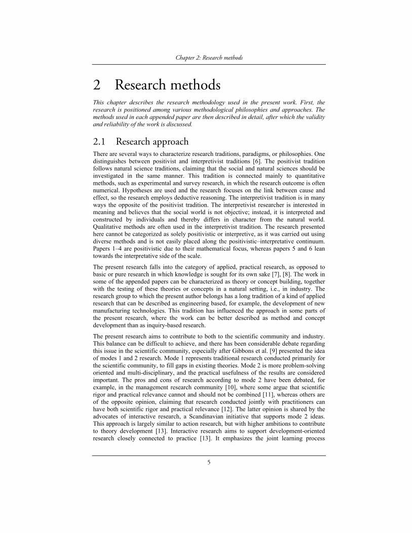
2 Research methods This chapter describes the research methodology used in the present work. First, the research is positioned among various methodological philosophies and approaches. The methods used in each appended paper are then described in detail, after which the validity and reliability of the work is discussed.

2.1 Research approach There are several ways to characterize research traditions, paradigms, or philosophies. One distinguishes between positivist and interpretivist traditions [6]. The positivist tradition follows natural science traditions, claiming that the social and natural sciences should be investigated in the same manner. This tradition is connected mainly to quantitative methods, such as experimental and survey research, in which the research outcome is often numerical. Hypotheses are used and the research focuses on the link between cause and effect, so the research employs deductive reasoning. The interpretivist tradition is in many ways the opposite of the positivist tradition. The interpretivist researcher is interested in meaning and believes that the social world is not objective; instead, it is interpreted and constructed by individuals and thereby differs in character from the natural world. Qualitative methods are often used in the interpretivist tradition. The research presented here cannot be categorized as solely positivistic or interpretive, as it was carried out using diverse methods and is not easily placed along the positivistic–interpretative continuum. Papers 1–4 are positivistic due to their mathematical focus, whereas papers 5 and 6 lean towards the interpretative side of the scale.

The present research falls into the category of applied, practical research, as opposed to basic or pure research in which knowledge is sought for its own sake [7], [8]. The work in some of the appended papers can be characterized as theory or concept building, together with the testing of these theories or concepts in a natural setting, i.e., in industry. The research group to which the present author belongs has a long tradition of a kind of applied research that can be described as engineering based, for example, the development of new manufacturing technologies. This tradition has influenced the approach in some parts of the present research, where the work can be better described as method and concept development than as inquiry-based research.

The present research aims to contribute to both to the scientific community and industry. This balance can be difficult to achieve, and there has been considerable debate regarding this issue in the scientific community, especially after Gibbons et al. [9] presented the idea of modes 1 and 2 research. Mode 1 represents traditional research conducted primarily for the scientific community, to fill gaps in existing theories. Mode 2 is more problem-solving oriented and multi-disciplinary, and the practical usefulness of the results are considered important. The pros and cons of research according to mode 2 have been debated, for example, in the management research community [10], where some argue that scientific rigor and practical relevance cannot and should not be combined [11], whereas others are of the opposite opinion, claiming that research conducted jointly with practitioners can have both scientific rigor and practical relevance [12]. The latter opinion is shared by the advocates of interactive research, a Scandinavian initiative that supports mode 2 ideas. This approach is largely similar to action research, but with higher ambitions to contribute to theory development [13]. Interactive research aims to support development-oriented research closely connected to practice [13]. It emphasizes the joint learning process


6

between researcher and practitioner [14] and can be characterized as research conducted with practitioners as opposed to traditional research, which is normally conducted on. In a similar vein, action research can be described as research conducted for [13]. Another way to address similar issues regarding lack of practical relevance is the industry-as-laboratory concept developed by Potts [15]. The concept originates from software engineering research, and its main idea is that the research process entails constant interaction between researcher and practitioner in which the solutions developed by the researcher are constantly evaluated in the “real world”. The work presented here has not been carried out strictly according to any of these approaches, but the ideas in these interactive approaches about the importance of practical relevance are considered crucial throughout the thesis. The author believes that, in the field of manufacturing systems, there is a need for research with a clear focus on practical relevance, because of the highly applied nature of the field. Manufacturing systems research is also often practice oriented, aiming, for example, to improve design, analysis, and improvement methods in order to increase industry competitiveness. The research presented here was conducted mainly within the VINNOVA-financed TESSPA and Lean Wood Engineering research projects, and based on the results from the SSF-financed Shortcut project. All these are projects in which university–industry collaboration was a precondition for financing. This collaborative aspect has made practical relevance a natural part of the research process. A risk of research conducted in close collaboration with practitioners is that it may move in a direction resembling consultancy work rather than scientific research, but as stated earlier, this thesis aims to combine scientific and practical relevance. Scientific relevance has been considered, for example, by reviewing the literature to ensure the uniqueness of the work.

The research process for this thesis entailed developing models and concepts, and testing them in real-world settings in various ways. The procedure is largely similar to a framework developed for applied research in the systems development field [16]. This framework includes several research activities that can be both positivistic and interpretive. A model of the framework is shown in Figure 2.1, in which theory building, observation, and experimentation represent different methods used to develop a prototype that constitutes both a proof of concept and a basis for continuing research. This procedure is somewhat similar to the industry-as-laboratory approach, as both seek to ensure the practical relevance of research by iteratively testing their concepts in industry. Though the present work is not systems development, it comprises similar activities, encompassing both model development and the industrial conditions for the models, including prototype development. The various methods used relate to the two research questions. Some of the work presented here constitutes theory building as presented in Figure 2.1, some observation and experimentation, and some prototyping. Section 2.2 will present the research methodology in greater detail, describing and categorizing each paper with reference to the model presented in Figure 2.1.


7

Figure 2.1: Methodological approach to information systems research, adapted from Nunamaker et al. [16].

2.2 Methodological description of the appended papers The first three papers are model oriented, are clearly related to the first research question (RQ1), and lean primarily toward theory-building as shown in Figure 2.1. The three subsequent papers are primarily linked to the second research question (RQ2).

Paper 1: A general economic model for manufacturing cost simulation This paper presents a mathematical model for making manufacturing cost calculations. The origin of the model was a belief that the manufacturing industry lacked appropriate methods for analyzing its manufacturing systems from a cost perspective, not least when it came to outsourcing decisions. The problem formulation that led to the formulation of RQ1 originated from industry experience, but the model was developed simultaneously with the literature study in order to investigate the scientific relevance of the problem. The literature study reviewed the literature on manufacturing costs, manufacturing cost models, and cost accounting. The main purpose of the developed model was to link production performance parameters to cost parameters. This would produce a tool for analyzing current manufacturing systems and simulating future scenarios, consequently raising cost consciousness in the manufacturing department. The solution to the problem formulation partly originates from a method developed by Ståhl [17] for collecting and analyzing losses in downtime, quality, and production rate in manufacturing systems. Using this method, data regarding the quantity and the causes of the losses are systematically collected. Results from implementing that model in various companies indicated that these performance losses were often large. Because these losses directly affect production time and the quantity of scrapped parts, they also affect costs, and were therefore considered necessary parameters of the cost model. The cost model presented here can be viewed as building on the method developed by Ståhl [17], in which the results of data collected by the use of the method become part of the input data for the cost model, allowing the costs of specific loss causes to be calculated. These ideas for a production analysis method including a cost perspective, in combination with the results of a literature study of existing cost models, resulted in the model described in Paper 1. The three previously mentioned

Theory buildingConceptual frameworks,

mathematical models, and methods

System developmentprototyping

Product development and technology transfer

ExperimentationComputer simulation,

field experiments, and labexperiments

ObservationCase studies, survey

studies, and field studies


8

losses constitute central parameters of the cost model, and the resulting connection between these losses and their costs is what makes the model original.

The cost model is in the paper exemplified by hypothetical data, i.e., no specific empirical data were used when working on this paper. Besides the mathematical model, the paper also suggests how the model can be used in practice. The paper fits well into the theory building category shown in Figure 2.1.

Paper 2: Relations between volume flexibility and part cost in assembly lines This paper describes how the cost model presented in Paper 1 can be used to analyze volume flexibility in an assembly line from a cost perspective. The idea for the paper originated from a case study of the development of a flexible assembly line, in which the number of operators could be varied to meet varying demands in production volume. In studying the line, the idea emerged of using the cost model presented in Paper 1 to analyze how such flexibility affects the assembly cost. A literature review on volume flexibility and its relationship to costs was conducted to ensure that the problem was also of interest from a scientific perspective.

The data collected during the case study and the configuration of the studied assembly line were used in developing the concept presented in Paper 2. The empirical data come from observations of the assembly line and from interviews, and were gathered to gain an understanding of the assembly line characteristics. The paper includes a modified version of the model presented in Paper 1, based on the collected empirical data regarding the characteristics of the studied line. As in Paper 1, the work presented in this paper originated from problems found in practice. Using the framework presented in Figure 2.1, the paper can be categorized as a combination of theory building and observation, with an emphasis on theory building.

Paper 3: Dynamic manufacturing costs - describing the dynamic behavior of downtimes from a cost perspective Paper 3 is somewhat similar to Paper 2, as it also describes a new application area for the cost model presented in Paper 1. The concept for the work presented in the paper was not based on any specific empirical findings, but is presented here using data from a company. The data consist mainly of downtime data extracted from the company’s downtime collection system, and of cycle time data and cost data regarding material, wages, and equipment. Real data were used to ensure that the results would be representative of real-world conditions. A literature review on downtime variability and downtime costs was conducted to relate the proposed approach to existing research in the field. Using the framework presented in Figure 2.1, the paper can be categorized as theory building, with some elements of observation due to the use of real data.

Paper 4: Implementation of an economic model to simulate manufacturing costs This paper applies the cost model developed in Paper 1 in an industrial setting. The study tests the applicability of the model in a real-world case, thereby investigating how it could be applied in practice. A manufacturing cell in an automotive company was selected for the study. The company was regarded as an intended typical user of the model in terms of production configuration (i.e., batch production divided into several processing steps) and products (i.e., products entailing significant manufacturing costs). The study started by defining and characterizing the cell in relation to the model parameters by means of observations and interviews. Input data for the model were then collected by means of observations and from databases (in the case of cost-related data). The observations were made using the production performance matrix (PPM) concept (see section 3.1.2.1) to


9

gather data on manufacturing performance parameters, comprising downtimes, scrapped parts, along with the registration of the causes of those losses, and setup time. This paper constitutes observations as presented in Figure 2.1.

Paper 5: Conditions for and development of an IT-support tool for manufacturing costs calculations and analyses Paper 5 investigates the conditions for the industrial use of the cost model and describes a prototype software application of the model. The conditions were investigated in two studies. The first study investigated the functionality of various commercial manufacturing performance data collection systems in terms of their support of the collection of the data required for the cost model. The second study investigated whether manufacturing companies were indeed collecting the required data. The first study investigated four data collection systems by interviewing the relevant software suppliers. The interviews were semi-structured and aimed at mapping the performance of the systems. The second study was conducted by visiting five manufacturing companies to evaluate their performance data collection systems by means of semi-structured interviews. The purpose of these studies was not to obtain generalizable results, but rather to gain an idea of the prevailing conditions. The software products chosen for the first study were based mainly on the software products used by the companies collaborating in the TESSPA project. Companies participating in that project, with one exception, also constituted the participating companies in the second study. The software prototype was developed in collaboration with an intended user of the software. The collaboration ensured that the prototype would be developed based on real-world conditions in terms of, for example, data storage and parameter definitions. The purpose of developing the software application was to explore the requirements for a user-friendly software application of the cost model, what functions it should include, and how the results could be presented and visualized. Using the framework presented in Figure 2.1, the paper can be categorized as a combination of observation and system development prototyping.

Paper 6: Availability improvement by structured data collection: a study at a sawmill Paper 6 investigates how the detail level of the downtime data companies collect for follow-up and analysis of availability affects data usability and examines how the operators responsible for data collection perceive changes in the level of data detail. This study used an interactive approach and was conducted at a sawmill company. It was interactive in the sense that the researcher and company personnel jointly developed a new structure for grouping the various downtime causes available in the downtime data collection system used by the company. In addition, new downtime causes were added to the new structure to increase the detail level of the collected data. The new structure was based on a structure found in the PPM concept, developed by Ståhl [17] and described in section 3.1.2.1. This structure was presented to the production manager and the most experienced maintenance worker in the company. The original structure was then modified and new downtime causes were formulated, based on the experience of these two company representatives and the present author. The new structure was immediately put into use in one section of the sawmill. After it had been used a few months, operators and the production manager were interviewed. The operator interviews concerned their experience of registering downtimes based on the new structure and the increased number of downtime causes. The interview with the production manager concerned whether the higher level of detail in downtime causes affected the knowledge gained from the collected data. This paper fits into the observation category presented in Figure 2.1.


10

Additional model development not included in the appended papers Section 4.2 describes developments of the cost model presented in Paper 1, including enhanced equations for calculating downtime and equipment costs. There is a major difference between planned and unplanned downtimes regarding their link to manufacturing performance and when they occur. This knowledge evolved during the course of the PhD project and was therefore not considered sufficiently in Paper 1. When implementing the model in industry, it was realized that equipment costs were the most difficult to determine with desired accuracy. Every company has its own opinion as to how these costs should be calculated, for example, concerning what costs to include and the time frame on which to base depreciation calculations. Hence, it was considered necessary to define the two equipment cost parameters of the cost model in greater detail, suitable for the type of analysis for which the cost model is intended. The proposed hourly equipment cost expressions were developed based on literature studies of the subject. The section largely constitutes theory building and fits into the theory building category presented in Figure 2.1.

2.3 Validity and reliability Two common parameters used to describe the quality of research work are validity and reliability.

Validity Validity relates to accuracy, i.e., whether the research instrument measures what it is designed to measure [6]. This is a fairly complex term for which several definitions can be found in the literature. Yin [18] lists three types of validity: construct validity, internal validity, and external validity. Construct validity is about constructing correct operative measures of the phenomenon being studied and avoiding subjective judgments in the data collection phase. Internal validity concerns the establishment of causal relationships in which one demonstrates that certain conditions lead to other conditions (this applies only to explanatory and causal studies). External validity is equivalent to generalizability and describes the extent to which a study can be generalized.

The construct validity of papers 1–3, characterized by method and model development, is strengthened by literature studies, in which the proposed methods and models are compared with similar findings in the literature. The thesis also describes implementations of these methods and models in an industrial context to strengthen the construct validity. For the work presented in Paper 6, the construct validity was considered by interviewing several people in the company and by holding ongoing discussions of the research with company representatives. The construct validity of this thesis is also strengthened by the fact that results were presented in international conferences that included review procedures and in peer-reviewed scientific journals.

Internal validity is mainly applicable in the work presented in Paper 6, which includes a pre-experiment that can be described as a one-shot case study. This is generally viewed as the weakest form of experiment because the parameters included are not controlled. This study design was used because the interviews conducted after the change focused on comparisons between the old and the new downtime collection structures, concerning how the respondents experienced the change, so no causal relationships were established.

Yin [18] claims there are two types of generalizations, statistical and analytical. Statistical generalization is perhaps the most obvious type, and describes how generalizations can be extended to a population from a sample. Analytical generalization refers to the


11

generalization of results into a theory and not to a population. The generalizations made in this thesis are based on analytical generalization. The proposed mathematical models and methods are designed to be applicable in the area of discrete manufacturing. The aim has been to develop general models and methods in this area, though, as various implementations have demonstrated, minor adjustments of the mathematical models have to be made in every case.

Reliability Reliability describes the repeatability of the research, i.e., the degree to which one obtains the same results when repeating the research. Appended papers on model and method development cannot be described in terms of reliability as they are not based primarily on empirical findings. However, reliability is considered when implementing these concepts in industry, as described in papers 4–6. The data used in the implementations are stored in databases or written documents. The interviews conducted for the work described in Paper 6 are also stored in databases.

Chapter 3: Frame of reference

12

3 Frame of reference This chapter describes the frame of reference of the thesis. Because this thesis concerns the links between a manufacturing system’s technology, performance, and cost, the frame of reference focuses on these issues. It starts with work on performance and performance measurement in manufacturing systems; thereafter, various methods and models concerning manufacturing costs are described.

Since all of the work presented in this thesis concerns manufacturing system performance, in some respects, section 3.1 can be considered to be related to the entire work, except for section 3.1.2.3 on downtime registration, which is clearly linked to Paper 6. Section 3.2 on cost accounting, section 3.3 on manufacturing cost models, and section 3.4.1 on quality cost relate primarily to Paper 1, but also to papers 4 and 5. Section 3.4.2 on downtime variability and its costs relates to Paper 3 and section 3.4.3 on volume flexibility and its costs relates to Paper 2. Section 3.4.4 on equipment cost relates to the additional results presented in section 4.2.

3.1 Manufacturing system performance Manufacturing system performance is a broad topic including modeling techniques, methods for analyzing and improving the performance, and measurement system design. The performance literature reviewed below is clearly linked to the parameters included in the proposed cost model and covers theories of performance improvement and its relationships with costs, and performance measurement.

3.1.1 Theories of the relationship between performance improvement and cost

In 1990, Ferdows and De Meyer presented a model of manufacturing development called the sand cone model [19] (see Figure 3.1). The idea underlying the model is based on the assumption of Skinner [20] and many subsequent researchers that there are tradeoffs between various manufacturing capabilities, an increase in one leading to a decrease in another, meaning that a manufacturer cannot excel in all. The manufacturing capabilities in question are, above all, cost efficiency, quality, dependability, and flexibility. Ferdows and De Meyer found that not all companies encountered such tradeoffs, and the authors believe that this is due to the sequence in which the capabilities are improved. The sand cone model illustrates the appropriate sequence, according to Ferdows and De Meyer. In this model, quality is the basis: for lasting improvements in any other capability, quality must be considered first. Only when quality is acceptable can one also start to improve manufacturing dependability; thereafter, work on improving manufacturing speed (or flexibility) can begin. When effort has gone into increasing manufacturing speed, then cost efficiency programs can be started, although Ferdows and De Meyer claim that cost efficiency may be reduced due to improvements in other capabilities.


13

Figure 3.1: The sand cone model, adapted from Ferdows and De Meyer [19].

Whether this model is true, that is, whether the sequence suggested in the sand cone model is better than another, has been investigated extensively with mixed results [21]. According to Schroeder et al. [21], many previous evaluations of the model have been inadequate, as they have not really examined the suggested sequence but only established positive relationships between the capabilities. Schroeder et al. therefore conducted a new evaluation based on two types of tests considering the sequence, and found no consistent support for the sand cone model. Schroeder et al. believe that there might be a consistency effect, i.e., the best sequence could vary based on, for example, country and industry.

Besides the tradeoff and sand cone theories, other theories treat the same theme. Schmenner and Swink [22] have developed a theory of performance frontiers. The theory includes both the tradeoff and sand cone theories, concluding that both are valid, but in different situations. A performance frontier is defined as “the maximum performance that can be achieved by a manufacturing unit given a set of operating choices” [22]. The model includes two frontiers: the asset frontier and operating frontier. The asset frontier is altered by investments in manufacturing equipment, while the operating frontier is altered by changes in the operation procedures and policies of the manufacturing system given its existing asset frontier. Figure 3.2 depicts the theory. Figure 3.2 (a) shows the performance frontiers of two hypothetical plants, A and B. Both plants share the same asset frontier, i.e., the same equipment, but have different operating frontiers. The different operating frontiers suggest that the plants may have different management policies, plant B’s being more successful. Schmenner and Swink distinguish two types of movements within the operating space (i.e., within the operating frontier): improvement and betterment. Improvement is defined as improved performance in one or more dimensions without degradation in any other dimension, for example, by increasing efficiency or utilization; Figure 3.2 (b) illustrates this, A representing the condition before improvement. After improvement, the company has moved to the operating frontier, meaning that, from now on, further improvements will cause higher unit costs. Betterment is defined as any change in operation policies leading to a rightward movement of the operating frontier or to a new shape of the frontier. This is depicted in Figure 3.2 (b), which shows that betterments lead to a new operating frontier as the company moves from A1 to A2. Schmenner and Swink are saying that when a company is far away from its operating frontier, it can make improvements in one performance dimension without risk of degrading other dimensions, in accordance with the cumulative effect argued for in the sand cone theory. However, when the company has reached its operating frontier, then improvements in one performance dimension will likely cause degradation in other dimensions, i.e., tradeoff theory will then apply.

Cost efficiency

Speed

Dependability

Quality


14

Figure 3.2: (a) Performance of two companies with identical asset frontiers but different operating frontiers. (b) Improvement leading to a shift from A to A1 and a betterment leading to a shift from A1

to A2.

3.1.2 Performance measurement A performance measurement system (PMS) is defined by Neely et al. [23] as a “set of metrics used to quantify both the efficiency and effectiveness of actions.” Despite an extensive, decades-long PMS literature related to manufacturing, there has been a marked increase in publications in this field over the last 20 years [24]. According to Ghalayini and Noble [25], the PMS literature can be divided into two main phases, the first extending from the 1880s to the early 1990s and the second, or current phase, covering the period since then. In the first phase, financial measures were emphasized. In the current phase, considerable emphasis is placed on the shortcomings of traditional financial measures; the use of non-financial measures is advocated, although there is no clear consensus among authors as to what non-financial measures companies should select.

Neely et al. [23], in reviewing the PMS literature, distinguish four dimensions of performance measures, namely, quality, time, flexibility, and cost. These four dimensions describe what these authors found that the literature regarded as the most important dimensions in defining manufacturing performance. White [26], in his survey of performance measures, proposes a similar division, but as well as the four dimensions mentioned above, his also includes delivery reliability as a major dimension. White says that these five dimensions jointly constitute competitive capability, and adds four additional dimensions that describe various aspects of the measures, such as data source and type, as shown in Table 3.1.

Table 3.1: White’s five dimensions of a PMS.

Competitive capability

Data type Reference Orientation Data source

Cost Subjective Benchmark Process input Internal Quality Objective Self-referenced Process outcome External Flexibility Delivery reliability Speed

White concludes that most measures used by companies are internal, objective, and self-referenced, and have a process–outcome orientation. At the same time, he argues for the importance of companies’ also obtaining externally based, subjective, benchmark, and process input-oriented measures and not simply focusing on cost capabilities, as many companies have traditionally done.

Arguing as White does for multidimensional measures is common in the second phase of PMS research. Gomes et al. [27], in their review of the PMS literature, constructed a five-

A1A BAsset frontier

Operating frontier for A

Operating frontier for B

A

A2 Asset frontier

Operating frontier

Improved operating frontier Cost Cost

Performance Performance

(a) (b)


15

phase framework for the evolution of PMS. The framework they advocate suggests that development is headed toward multidimensional, balanced, and integrated measures, as well as toward acceptance of the importance of non-financial measures and of the connection between these measures and company strategy.

3.1.2.1 The production performance matrix (PPM) The production performance matrix (PPM) model for collecting and analyzing process-near losses has been developed by Ståhl [17] and is shown in Figure 3.3. This model was originally developed to analyze tool breakdowns in metal cutting, but has since also been used to analyze whole manufacturing systems. The performance parameters Q, S, and P represent the OEE parameters quality, availability, and performance efficiency, respectively. The groups A to H in the figure represent the causes of the disturbances involved. A benefit of this model is its structure, i.e., the division of the causes into different groups, which can facilitate both downtime registration and result analysis.

Figure 3.3: Structure for systematic analysis of manufacturing processes.

3.1.2.2 Overall equipment effectiveness (OEE) One measurement manufacturing companies often employ is overall equipment effectiveness (OEE). Nevertheless, the PMS literature seldom treats this measure, possibly because of the previously described emphasis on multidimensional measures in the PMS literature. OEE focuses on what Nakajima [4] calls the “six big losses” due to equipment failure, required setup time, idling and minor stoppages, reduced speed, quality defects, and reduced yield. As can be seen, OEE measures the performance of equipment on the shop floor. OEE is calculated by multiplying availability rate, A, by performance efficiency, P, and quality rate, Q. The rates are defined in equations 3.1 to 3.4.

Performance parameters

Groups of causes

Description Q1,..,Qn

(units)S1,...,Sn

(min)P1,...,Pn

(min)∑

A1,...,An Tool-related failures

B1,...,Bn Material-related failures

C1,...,Cn Machine-related failures

D1,...,Dn Failures related to personnel and organization

E1,...,En Maintenance-related factors

F1,...,Fn Specific process-related factors

G1,...,Gn Factors related to peripherals such as material handling equipment

H Unknown factors∑


16

amountprocessed

amountdefectamountprocessed Q 3.1

timeloading

timeoperatingA

3.2

The operating time is defined in Equation 3.3, in which loading time is total production time minus planned downtimes, such as planned maintenance and scheduled meetings. Unplanned downtimes result from, for example, failures, setup times, and time for die exchange.

downtime unplannedtimeloadingtimeoperating 3.3

timeoperating

timecycleidealamountprocessed P

3.4

Using White’s categorization as shown in Table 3.1, OEE then measures various aspects of quality, flexibility, and speed. OEE is also internal, objective, and self-referenced and measures process outcome. It fails, however, to use all the proposed dimensions of a measurement system and needs to be complemented by additional measures, as has also been noted by Jonsson and Lesshammar [28]. Another shortcoming of OEE is that it measures only the performance of individual pieces of equipment, failing to take account of the links between various machines and the flow of materials in the manufacturing system. This shortcoming of OEE has been identified by Jonsson and Lesshammar [28], Muchiri and Pintelon [29], and Muthia and Huang [30]. Muthia and Huang [30] propose a solution to the insufficiency of individually measuring pieces of equipment, introducing the term overall throughput effectiveness (OTE). OTE is based on OEE and can be described as a factory-level version of OEE that takes equipment dependability into account. OTE is expressed in four ways, depending on the characteristics of the layout of machines, such as whether they function in series or parallel.

In their review of the OEE literature, Muchiri and Pintelon [29] consider various suggested modifications of OEE, all of which attempt to overcome its various insufficiencies. The modified measures include production equipment effectiveness (PEE), overall asset effectiveness (OAE), overall plant effectiveness (OPE), and OTE. Muchiri and Pintelon [29] believe that the absence of a cost dimension is a serious shortcoming of OEE and that future research should explore the translation of equipment effectiveness into costs. They also believe that future research should investigate the benefits of investing in automated data collection systems to gather the data needed for OEE calculations.

3.1.2.3 Documenting downtime losses After Nakajima presented the OEE measure, several papers examined the subject, some proposing improvements to the original OEE definition. For example, Jeong and Phillips [31] extended Nakajima’s six losses to 10 losses, a schema they believe is more suitable in capital-intensive companies. The losses defined by Jeong and Phillips are: nonscheduled time, scheduled maintenance, unscheduled maintenance, R&D time, engineering usage time, setup and adjustment, WIP starvation time, idle time without operator, speed loss, and quality loss. Jeong and Phillips claim that a deficiency of the original OEE definition


17

is that planned downtime, such as planned maintenance, is not considered a downtime loss. They believe that as planned downtimes are crucial to capital-intensive companies, these must be included in OEE. They acknowledge that the accuracy of the OEE measure depends on the quality of the collected input data. The available downtime causes to choose from in a computerized collection system must be well defined, which calls for careful collection system design.

Bamber et al. [32] advocate the use of cross-functional teams to improve OEE figures, because they believe that several competences, for example, maintenance, production, and quality, are needed for successful improvement work. In their case study, the OEE monitoring apparently consisted solely of time data without any data describing the downtimes or their causes. This means that the OEE figures were used only to measure the performance; the causes underlying the losses had to be found when developing the cause–effect diagram. Dal et al. [33] describe OEE implementation by an airbag manufacturer. Operators documented the downtime losses by recording the durations and descriptions of the downtimes on a record sheet. They also discuss the importance of accurate data: data must be convincing to production management, otherwise they will not be used effectively. Ljungberg [34] also discusses the importance of data collection, claiming that data collection problems have been insufficiently treated in the literature. Such problems include poor data collection systems—which must be fast but still accurate—and resistance on the parts of operators and foremen to collecting the data. This resistance can be decreased, according to Ljungberg, by designing the data collection system together with the users, an approach also mentioned by Gibbons and Burgess [35]. Resistance can also be decreased if users are helped to understand how the data are actually compiled and used, according to Ljungberg. Ljungberg [34] also discusses the pros and cons of registering the losses using pen-and-paper versus computerized systems. Pen-and-paper solutions are simpler than computerized systems, but the recorded downtime durations will not be completely accurate. A computerized system can register correct downtime durations, and some systems even force the operator to register a downtime cause before the equipment can be restarted, meaning that all losses will be registered. However, such software systems can be expensive and difficult to use. A computerized system in which the operator registers failure number and type while the computer keeps track of the downtime and the actual cycle time is recommended. Ljungberg’s OEE measurements used five independent variables to categorize the cause of every recorded loss; these variables were production process, process knowledge, maintenance activities, external factors, and production conditions.

Wang and Pan [36] recommend computerized data collection in which the operator chooses a specific downtime cause to describe the failure. They present an example from the semiconductor industry in which seven downtime causes are available. They also demonstrate how a cause–effect diagram can be used to determine more detailed downtime causes. How the collected data are or should be used is not considered. Andersson and Bellgran [37] have compared manual and automatic downtime registration in a company having both systems. They too declare the advantages of an automatic system, its only disadvantages being investment and licensing costs and setup time.

Some non-OEE-related literature also considers downtime registration. For example, De Smet et al. [38] describe various case studies of disturbance registration. In one case, the downtime causes from which the operator could choose when registering a failure were too general and vague. Operators could also supply additional explanation in a comment line, but did not use this feature satisfactorily. Consequently, a more relevant and detailed list of


18

causes was developed for each machine, and feedback was given to the people who registered the failures to motivate them to better describe the failures.

3.2 Cost accounting methods In Swedish industry, the principles of cost accounting stem from a model presented in 1936 called “Enhetliga principer för självkostnadskalkylering” [39]. The model is often called EP and is used for absorption costing, i.e., a method for distributing all costs generated in the company down to every produced product. In this model, the cost items are as follows:

Direct material cost Indirect material cost Direct labor cost Manufacturing overhead costs Special direct costs Cost of sales Administration costs

In EP, manufacturing overhead costs are divided into costs closely connected to manufacturing and costs that are not. The first group includes costs such as those of maintenance, additives, energy, equipment, building, and employees in the manufacturing department. The second group includes costs such as design department, patent, and laboratory costs. According to EP, manufacturing overhead costs are allocated based on direct material, direct labor, labor hours, or machine hours.

3.2.1 Activity-based costing (ABC) According to Kaplan and Anderson [40], activity-based costing (ABC) corrected some of the problems found in traditional cost accounting. The traditional cost accounting model was developed at a time when direct labor constituted a larger part of the total cost than it does today, meaning that direct labor has become an increasingly worse allocation key for overhead costs. Furthermore, companies have shifted from mass production strategies to more flexible, customer-focused strategies, resulting in increased overhead costs. According to Plowman [41], when traditional cost accounting was developed, overhead costs constituted such a small proportion of the total cost that it was not seen as worthwhile to have a system that more accurately captured the proportion of the overhead costs associated with each product. Distributing the overhead costs based on, for example, direct labor was in this context seen as simple and sufficiently correct.

ABC is a method aiming to allocate overhead costs more correctly by tracing these costs to activities and then connecting the activity costs to the order, product, or customer levels. Instead of grouping several activities into an overhead cost pool, such as manufacturing overhead, the cost item is segregated into several activities [42]. ABC can be divided into two stages. The first entails allocating costs based on the main activities occurring in various departments to form activity cost pools, called resource cost drivers. The second stage entails allocating these costs to cost objects (e.g., products, customers, or any chosen unit of analysis) by identifying activity cost drivers. See Figure 3.4 for a generic model of the process.


19

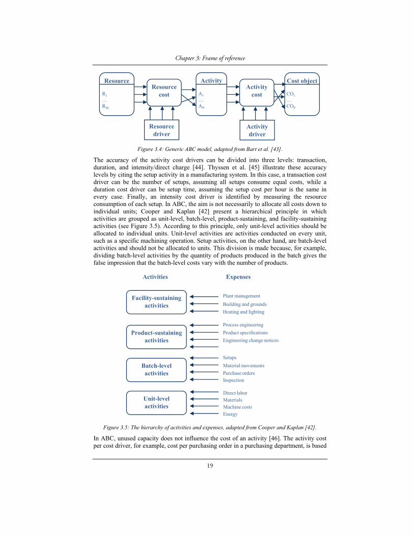
Figure 3.4: Generic ABC model, adapted from Bart et al. [43].

The accuracy of the activity cost drivers can be divided into three levels: transaction, duration, and intensity/direct charge [44]. Thyssen et al. [45] illustrate these accuracy levels by citing the setup activity in a manufacturing system. In this case, a transaction cost driver can be the number of setups, assuming all setups consume equal costs, while a duration cost driver can be setup time, assuming the setup cost per hour is the same in every case. Finally, an intensity cost driver is identified by measuring the resource consumption of each setup. In ABC, the aim is not necessarily to allocate all costs down to individual units; Cooper and Kaplan [42] present a hierarchical principle in which activities are grouped as unit-level, batch-level, product-sustaining, and facility-sustaining activities (see Figure 3.5). According to this principle, only unit-level activities should be allocated to individual units. Unit-level activities are activities conducted on every unit, such as a specific machining operation. Setup activities, on the other hand, are batch-level activities and should not be allocated to units. This division is made because, for example, dividing batch-level activities by the quantity of products produced in the batch gives the false impression that the batch-level costs vary with the number of products.

Figure 3.5: The hierarchy of activities and expenses, adapted from Cooper and Kaplan [42].

In ABC, unused capacity does not influence the cost of an activity [46]. The activity cost per cost driver, for example, cost per purchasing order in a purchasing department, is based

Resource

R1

…RM

Resourcecost

Activity

A1

…AN

Activitycost

Cost object

CO1

…COP

Resourcedriver

Activitydriver

Unit-level activities

Direct laborMaterialsMachine costsEnergy

Batch-levelactivities

Setups

Material movements

Purchase ordersInspection

Product-sustainingactivities

Process engineering

Product specifications

Engineering change notices

Facility-sustainingactivities

Plant management

Building and grounds

Heating and lighting

Activities Expenses


20

on the available resources, i.e., the practical number of purchase orders the department can handle based on the resources available to purchasing staff. The cost of supplied resources of an activity can consequently be described as:

Cost of activity supplied = Cost of activity used + cost of unused capacity

This does not mean that the cost of unused capacity is neglected in ABC. Unused capacity cost indicates a mismatch between supplied and used resources, which the company should reduce by either reducing the quantity of supplied resources or exploiting the unused capacity, for example, by producing a new product.

Some years after the first papers on ABC were published, a variant of ABC evolved called activity-based management (ABM). ABM focuses on processes instead of products, using ABC data for performance measurements [47]. Figure 3.6 depicts the difference between ABC and ABM.

Figure 3.6: The difference in perspective between ABC and ABM.

In 2007, Kaplan and Anderson released a book in which they presented the concept of time-driven activity-based costing (TDABC) [40]. TDABC was developed because many users found traditional ABC too time-consuming to implement, sustain, and modify. Many users also doubted the accuracy of the resulting cost calculations. The principle of TDABC can be divided into two steps. The first entails calculating the cost of a specific resource, for example, a purchasing department. This cost is then divided by the available capacity in terms of time, giving the capacity cost rate. The next step is to estimate the time required for specific activities, for example, the time required to process a particular order. The cost of processing this order is then calculated by multiplying the capacity cost rate by the processing time. The cost of a process comprising several activities, for example, the manufacturing cost of a product produced using several machines, is calculated by building a time equation including the capacity cost rates and processing times of every machine used. The numerator of the capacity cost rate should include the costs of all resources required for the employee or equipment to perform the work. In many examples cited by Kaplan and Anderson [40], the capacity cost constitutes the cost of a department in the company—this is considered the simplest way to calculate the capacity cost. However, the authors also acknowledge that department cost can sometime be insufficient, for example, if some of a department’s resources are used by only one product. In such cases, the department cost can be divided into several process costs.

The denominator of the capacity cost rate, i.e., the capacity, should be the practical capacity, meaning the theoretical capacity minus breaks, training, education, repairs, and

Resources

Activities

Costobject

Performance measures

Costdrivers

ABC

ABM


21

maintenance. Although this concept is called time-driven ABC, Kaplan and Anderson [40] acknowledge that not all capacity cost rates should be based on time; sometimes, for example, square meters may be a better choice of dominator.

TDABC is considered to reduce the time spent collecting data, because changes only need to be made when resource cost or processing time changes. The accuracy is also considered to increase because staff no longer need to estimate the proportion of their time spent on specific activities.

3.2.2 Throughput accounting Another cost accounting method sometimes mentioned alongside ABC as an example of a new cost accounting concept is throughput accounting (TA), a method based on the theory of constraints (TOC). TOC was developed by Goldratt, among others, in the 1980s; the first ideas that would form the concept were introduced in The Goal [48] and have since been developed further in several papers. According to Rahman [49], TOC can be summarized by the following statements: “every system must have at least one constraint” and “the existence of constraints represents opportunities for improvement.” Constraints determine the performance limits of an organization: without any constraints, a profit-generating organization would have unlimited profits. According to Dugdale and Jones [50], there is no consistent TA theory, as the approach has been developed in parallel by various authors. Some regard TA as based on Goldratt’s theoretical work, while others associate TA with the work of Galloway and Waldron.

Goldratt’s theory includes three operational measures: throughput (T), inventory (I), and operating expense (OE) [51]. T is the sales revenue less the total variable cost, I is the total money invested in the products in inventory, and OE is the non-variable costs spent turning inventory into throughput. Based on these measures, net profit (NP) and return on investment (ROI) can be calculated. NP is defined as T – I and ROI as NP/I.

According to Dugdale and Jones [50], Galloway and Waldron are the key figures in developing TA. Central to TA is the rate at which businesses earn money, and the focus is on maximizing the return per bottleneck hour. In Galloway and Waldron’s version of TA, all costs, except material cost, are viewed as fixed costs in the short term, referred to in TA as total factory cost (TFC). The rate at which a product generates money is central to TA, and this rate determines a product’s profitability in relation to other products. A product’s absolute profitability is the relationship between its profitability rate and cost rate. TA ranks products according to the TA ratio, which is defined by equations 3.5 to 3.7. The return per factory hour is defined as:

resourcekey on Time

cost MaterialSalespricehourfactory per Return

3.5

The cost per factory hour is defined as:

resourcekey on available timeTotal

costfactory Totalhourfactory per Cost 3.6

Based on equations 3.5 and 3.6, the TA ratio is:

hourfactory per Cost

hourfactory per Return ratioTA

3.7


22

Galloway and Waldron developed their view of TA over several years, and in that time they abandoned some of their previous ideas and added others. A later contribution was T/TFC, an overall process measure defined as:

costfactory Total

ThroughputT/TFC

3.8

In T/TFC, throughput is defined as the contribution margin after material cost, and total factory cost as all the costs occurring except for material cost.

3.2.3 Life cycle costing Woodward [52] describes life cycle costing (LCC) as a method that “seeks to optimize the cost of acquiring, owning, and operating physical assets over their useful lives by attempting to identify and quantify all the significant costs involved in that life by the use of the present value technique.” The method was originally used by the US Department of Defense in the 1960s, but has since been applied in many other contexts, such as consumer products, equipment acquisition in manufacturing companies, and building acquisition [52], [53]. Woodward presents [52] an overview of the LCC concept, primarily in the equipment acquisition context, identifying the following elements:

Initial capital costs, including purchase costs, acquisition/finance costs, and installation/training costs

Life of asset Discount rate Operating and maintenance costs: the former include direct and indirect costs of

labor and materials, direct expenses, and establishment costs; the latter include direct labor, materials, fuel, equipment, and purchased services

Disposal cost Information and feedback Uncertainty and sensitivity analysis

The German VDMA 34160 standard, “Forecasting model for lifecycle costs of machines and plants” [54], includes a comprehensive list of items influencing the cost of a machine throughout its life cycle. The various cost items are grouped into three phases, the preparatory, operating, and further utilization phases, each including different cost pools containing various constituent parameters. The phases and their cost pools are listed below:

Preparatory phase

Acquisition Infrastructure costs Other preparatory costs

Operating phase

Maintenance and inspection Repairs Unscheduled repairs Occupancy costs Material costs Energy costs Production and process materials Disposal costs


23

Personnel costs Tool costs Setup costs Warehousing costs Other operating costs

Further utilization phase

Dismantling Residual value Other further utilization costs

The standard also includes formulas for calculating the values of the cost pools based on the cost items and parameters listed for each cost pool.

An example of LCC implementation is described by Folgado et al. [55]. In this case study, LCC is used to compare two mould manufacturing alternatives. The total cost is divided into three categories: process cost (i.e., machine and labor), material cost (i.e., raw materials, standard components, disposable tools, and other consumables), and energy costs (i.e., energy consumed by the equipment). Other input parameters are times (e.g., setup and operation), equipment availability, production volume, and batch size. Any equations for the cost calculations are not presented.

3.2.4 Kaizen costing Kaizen costing is a cost management concept that originated in Japan. In Japan, it is often used together with target costing, a Japanese cost management concept used to reduce costs in product development. After this phase, the focus shifts to reducing the current manufacturing costs of a product, and it is in this phase that kaizen costing is employed. The main purpose of kaizen costing is to achieve ongoing cost reduction by periodically setting cost reduction goals for manufacturing processes. Lee and Monden [5] have described the use of kaizen costing in a Japanese company. The studied company set annual cost reduction targets for its plants as part of the budget process. These targets are broken down into cost reduction targets for specific processes in the plant. The cost reduction targets for the processes are then translated into improvement actions. Monden and Hamada [56] take a cost reduction target for a manufacturing department as an example. In this case, cost reduction can be realized in two ways: reducing labor cost by increasing capacity availability or reducing workforce size. The availability increase is then further divided into goals for specific processes, for example, goals for setup time reduction and machine breakdown reduction. According to Lee and Monden [5], fairly simple cost accounting methods can be used for the cost calculations.

3.2.5 Resource consumption accounting Resource consumption accounting (RCA) is a new accounting method, conceived circa 2000 [57]. It is promoted as a method combining the best of the German accounting tradition and ABC. According to Clinton and Webber [58], cost management in the USA and German-speaking countries belongs to different traditions. In the USA, cost management is highly influenced by financial accounting and external accounting, which has led to simpler accounting systems than those in many other developed countries. According to White [59], RCA is an accounting system that focuses on the manager and not the external financial statement. RCA represents an attempt to integrate the best ideas


24

from the German tradition, internationally often called GPK, with existing ideas from the USA, for example, ABC.

Resource flows and pools are central concepts in RCA. The resources flow between resource pools and to products. A resource pool (i.e., cost pool) needs specific inputs to produce an output, which can in turn support another cost pool or a product or service for a customer. It is important that the flows be modeled correctly, because one objective of RCA is to provide managers with cause-and-effect information so they can make the right decisions. Another central principle is responsiveness. This principle acknowledges that the relationship between resource pools can include both fixed and proportional costs and that the nature of the costs can change between pools. An example of this is electricity: it comes to the company as a proportional cost, but in some resource pools it becomes a fixed cost, for example, the cost of heating and lighting a manufacturing plant. The opposite of responsiveness is variability, i.e., that there is a clear relationship between total cost and total volume [59].

In RCA, only the costs of resources used should be allocated to products; the costs of idle capacity should be acknowledged but not affect the product cost. Costs of idle capacity should be attributed to the person or department responsible for them. Causality between resources and resource drivers are considered important. If causality cannot be determined, for example, regarding idle capacity, the costs should not be allocated to products [58]. Causality entails a cause–effect relationship between cost pools. If costs in one cost pool do not influence those in another cost pool or product, no such relationship should be included in the cost model, i.e., no arbitrary allocation should be made. The causality between resources and between resources and products should be based on non-cost quantitative relationships, i.e., not on percentages or other arbitrary principles [59].

RCA recommends that depreciation costs should be calculated based on replacement cost. If the same product is made using two different machines, one older than the other, the product cost should be the same [58].

3.3 Manufacturing cost models Besides the general cost accounting methods mentioned above, several papers describe more detailed cost models that capture the costs related solely to the manufacturing system, not attempting to be full cost models. These models can be classified in various ways depending on their characteristics; according to Tipnis et al. [60], these models can be divided into microeconomic and macroeconomic models. The microeconomic models describe specific process parameters influencing the part cost. Microeconomic models dealing with machining have been described, for example, by Colding [61], [62] and Alberti et al. [63], while Knight et al. [64] have developed a corresponding model for forging. In the machining field, a microeconomic model can describe how, for example, the cutting rate or feed influences the part cost. Macroeconomic models tend to aggregate parameters, for example, when cost calculations are based on the cycle time and not on the individual factors influencing the cycle time. Another distinction that can be made is between product cost-estimation models and models describing the historic cost of products already in production. The product cost-estimation models attempt to estimate primarily the manufacturing costs of products before they are put into production. A widely cited paper in this area is one by Shehab and Abdalla [65], which describes a knowledge-based system that can propose manufacturing methods and estimate product manufacturing costs based on a set of design and production parameters. For a review of various product cost-estimation techniques, see Niazi et al.


25

[66]. Eleven manufacturing cost models will be described below; the first three are based on ABC while the others are not based on any specific accounting method.

Koltai et al. [67] have developed a cost model based on ABC for calculating costs in flexible manufacturing systems (FMSs). One argument for developing the model was that the increasing overhead costs relating to the use of FMS cells render traditional accounting systems unsuitable. Another argument was that the cost model should consider the flexibility of FMSs, for example, the cost impacts of various production routes and setup times. In their ABC model, Koltai et al. [67] have focused on overhead costs, dividing these into five activity centers: tooling, loading/unloading, material handling, inventory, and other overheads. The tooling cost is allocated to products based on the number of tools used. The loading/unloading cost is allocated based on the order size. The material handling cost is allocated based on the use of material handling equipment, determined based on the distance travelled by the orders. The inventory cost is allocated to products based on order completion time. The overhead cost center consists of costs of maintenance, quality control, depreciation, etc., and is allocated based on order processing time. It can be concluded that, though the allocation principles used are fairly detailed, the model includes too few cost items to function as a complete manufacturing cost model; notably, no performance parameters are included.

Özbayrak et al. [68] have also developed an ABC model for an FMS cell. The model is used to determine the manufacturing and product costs for a manufacturing system that employs either the material requirement planning (MRP) strategy or the just-in-time (JIT) strategy. The FMS cell cited as an example in the paper is a simulation model and not a real system. The FMS cell is divided into six activity centers: workstations, inspection station, assembly line, setup activities, and robot and AGV systems. The resource costs distributed to the activity centers are: machines and cutting tool holders, computer system, robot and AGV system, automated storage and retrieval (AS/RS) system, fixed assets, externally provided resources (e.g., fuel for heating and electricity for lighting and ventilation), direct and indirect labor, insurance and indirect material, cutting tools and fixtures, direct energy consumption, direct material, and other services (i.e., costs of non-manufacturing services). These costs are divided into direct and indirect costs when they are distributed to the activity centers. The direct costs are directly distributed to the activity centers while the indirect costs are distributed based on utilization levels obtained from system simulation results. The investment cost of workstations is assumed to be a direct cost while the investment costs of the other equipment are assumed to be indirect costs. The investment costs are calculated as hourly costs by dividing the investment cost by the estimated economic life of the investment in hours. The calculations to convert the activity centers to unit costs are made using a unit cost equation. The equation calculates the cost per part by taking specific part characteristics, such as processing time, into consideration. Table 3.2 and the following equations describe the model.

Table 3.2: Cost parameters of the Özbayrak et al. model.

j Part level index DMCR[a(ij,o)] Direct machining cost rate ij Part i at level j ACR[a(ij,o)] Assembly cost rate R(ij) Part route DACR[a(ij,o)] Direct assembly cost rate o Operation index HC(ij) Handling cost S(ij,o) Standard setup time dR(ij) Distance route B(ij) Batch size of ij spAVG Speed of AGV vehicle a Activity index StC(ij) Storage cost OSCR[a(ij,o)] Overall setup cost rate w(ij) Average waiting time DSCR[a(ij,o)] Direct setup cost rate M(ij) Unit material cost t(ij,o) Processing time W(ij) Weight of material MCR[a(ij,o)] Machine tool cost rate


26

The setup cost includes both an hourly rate and a direct cost and is defined as:

ijR

ojj

j

joiaDSCRoiaOSCR

iB

oiS

1

)],([)],([)(

),(cost Setup

3.9

Even the machining cost includes both an hourly rate and a direct cost and is defined as:

)],([)],([),(cost Machining oiaDMCRoiaMCRoit jjj 3.10

The equation for the assembly cost is similar to that for the machining cost and is defined as:

)],([)],([),(costAssembly oiaDACRoiaACRoiA jjj 3.11

The handling and storage cost is defined as:

)()()(cost storage and Handling)(

jjAVG

iRj iwiDACStC

sp

diHC j 3.12

The material cost is defined as:

)()(cost Material jj iWiM 3.13

In the paper [68], Özbayrak et al. say that they also consider losses such as scrapping, reworking, and downtime, but do not describe exactly how these losses are treated.

Aderoba [69] has developed an ABC estimation model for job shops. The activities in a job shop are classified as machine-based production, labor-intensive production, technical services, and administrative services. The model includes two model alternatives, depending on whether the production is mainly machine or labor based, the difference being that the former has more machine-related parameters. In the machine-based version, the machine cost is calculated based on the initial investment cost and the installation cost. These costs are divided by the total number of expected operation hours. This rate is then multiplied by a factor greater than one, which takes account of maintenance, repair, and other costs related to the machine. Other production-related costs included in the model are floor space cost and utility cost. The model can be said to include several essential cost parameters, but no performance-related parameters.

Dhavale [70] has developed a cost model primarily for computer-integrated manufacturing systems (CIMSs). Dhavale argues that traditional cost accounting methods are inadequate in CIMS environments and describes three of their main shortcomings. One shortcoming is that direct labor has become a manufacturing overhead cost because operators cannot be easily identified with specific products: operators now operate several machines at the same time, each machine producing a different product. Another shortcoming is that since direct labor is a relatively small cost in CIMS-equipped versus conventional job shops, it has become inappropriate as an allocation basis for manufacturing overhead. Due to the small amount of direct labor in a CIMS environment, an error in assigning direct labor to a product has a greater impact on the overhead cost allocation than in a case with proportionally higher direct labor costs. The last shortcoming is that plant-wide manufacturing overhead pools are frequently used in traditional cost accounting systems. This means that all manufacturing overhead costs are put into just one cost pool, thereby ignoring the machines with which specific products are manufactured. Since machines usually differ in their share of the total overhead cost, the results can be fairly inaccurate.


27

The parameters included in the Dhavale cost model are presented in Table 3.3, after which the cost equations are presented.

Table 3.3: Parameters of the Dhavale model.

j Product index hli Expected production hours on machine i over its economic life

MCj Manufacturing cost of product j C2i Operating cost DMj Direct material cost UBD Annual operating cost i Machine index ai Fraction of total plant area occupied by

machine i hij Processing time in machine i hyi Expected production hours on machine i

this year ARi Application rate per machine hour C3i Personnel cost C1 Cost of capital expenditure PO Total annual personnel cost Mi Investment cost of machine i C4i Cost related to various service

departments ACC Total cost of accessories Si Annual service department costs allocated

to machine i mi Fraction of the total investment in machine i

The manufacturing cost of a product is calculated using Equation 3.14.

i

iijjj ARhDMMC )( 3.14

The application rate, ARi, consists of four cost groups: capital expenditure, costs related to the factory building, personnel costs, and costs related to various service departments. The cost equations for every cost group are presented in the paper [70]. The cost of capital expenditure, C1i, is calculated using Equation 3.15. The accessory cost parameter, ACC, includes the costs of central computing, automatic material handling, tools, fixtures, pallets, inspection, and assembly equipment.

i

iii hl

mACCMC

1 3.15

The operating cost, C2i, is formulated in Equation 3.16. UBD includes the costs of heating, electricity, water, custodial services, and building depreciation.

i

ii hy

aUBDC

2

3.16

The personnel cost, C3i, includes the costs of process analysts, maintenance, operators, systems manager, etc., and is formulated according to Equation 3.17.

i

ii hy

mPOC

3

3.17

The costs related to various service departments, C4i, for example, costs of personnel, design, and production engineering, are calculated using Equation 3.18.

i

ii hy

SC 4

3.18

Because the model does not include performance-related parameters, it is unsuitable for analyzing the performance of manufacturing systems.

Cauchick-Miguel and Coppini [71] developed a model for calculating the cost per piece in a manufacturing process, because they did not consider traditional accounting methods accurate enough for the current manufacturing environment. Cauchick-Miguel and Coppini


28

acknowledge that new accounting methods have emerged, such as ABC, but at the time of writing the paper, they believed that research into the advantages and disadvantages of ABC was inadequate, so they instead based their cost model on traditional costing systems. Their model is based on the cost center approach, but with the novel inclusion of two “contribution factors” intended to distinguish the costs related to each machine in situations in which the cost center comprises several machines. One contribution factor considers cost, productivity, and the number of machines in the cost center; the other considers technical parameters such as flexibility, automation level, and accuracy. Their approach is somewhat similar to the model proposed by Dhavale [70], as both models are based on cost centers and both propose using the relative cost of a specific machine as a way to allocate overhead costs to each machine. The Dhavale model, however, is slightly more detailed and includes two cost drivers, whereas the Cauchick-Miguel and Coppini model is based on only one cost driver. The paper also includes a more detailed cost model in which every machine constitutes a cost center. This model includes direct and indirect material, labor, machine, tool, inspection, overhead, and variable costs. Except for a fairly detailed expression for the tool cost, their work does not describe how the other costs should be calculated. The model includes only some aspects of performance-related costs, namely, inspection, reworking, and setup costs. The authors seem to believe that this detailed model would be too difficult to implement, so they instead propose a model based on contribution factors.

Noto La Diega et al. [72] have developed a cost model for FMSs based on a cost model presented by Alberti et al. [73]. What Nota La Diega et al. address is that in FMSs one cannot simply add the manufacturing costs of every operation to obtain the total cost. This is because the high variety of products and small batch sizes in FMSs result in varying utilization rates. Moreover, because of the high equipment cost in FMS, the utilization rate and general efficiency of the system become critical parameters in cost calculations. The part cost is based on five cost items: technological, logistics and control, tooling, specific, and opportunity costs. Opportunity costs are the costs of system utilization losses and are viewed as a consequence of choosing an FMS. The cost is formulated such that the part cost is lower if the part is produced in a mix constituting a well-balanced workload between workstations. By including the opportunity cost equation, a lower and upper bound can be formulated for the manufacturing cost, the lower bound describing a system with perfect balance between workstations. Besides the inclusion of an equation describing the costs related to balancing losses, the model lacks performance-related parameters.

Needy et al. [74] have developed a cost model for evaluating configuration alternatives for manufacturing cells. The cost model consists of only three factors: setup, material handling, and investment costs. The authors agree that more cost factors can be included, for example, labor costs and energy costs, but they believe that the more factors a cost model includes, the more prohibitively complicated and expensive it becomes to collect data and use the model. The cost is expressed as the cost for a specific planning period. This cost model permits the calculation of how the cost of introducing manufacturing cells into a job shop influences the total cost, which is the sum of the three mentioned cost factors. This model clearly contains too few parameters for the type of analyses addressed in this thesis.

Yamashina and Kubo have proposed a concept for cost-conscious manufacturing development called manufacturing cost deployment [75]. The concept includes a cost model in which the costs are divided into fixed and variable costs. The fixed costs consist only of depreciation costs; the variable costs include the costs of direct material, indirect material, direct labor, indirect labor, tool, die and jig, energy, and maintenance. The


29

authors then connect these costs to production losses. The identified losses are the following: breakdown, setup, tool change, startup, short stoppage, speed down, defects, management, operation motion, logistics, line organization, measurement, yield, indirect material, die and jig, and energy-related losses. For each type of loss, cost formulas are presented expressed in cost per part. The authors distinguish between time-related and physical losses, the former being measurable in terms of time and the latter in quantity. They also distinguish between the scenarios when the production capacity is smaller than the planned output quantity and when it is larger, depreciation only being included in the cost of time-related losses in the first case and energy and direct labor costs only being included in the second. This cost concept only describes the costs of losses, not the total manufacturing cost. For example, how the cost of defects in processing steps after the first should be calculated is not formulated; it is only mentioned that the costs for the previous steps should be considered. Manufacturing cost deployment is more than just cost formulas; it is a whole concept of how to implement improvement activities in a structured way. The concept is based largely on five matrixes, each having a specific function. The first one is used for identifying losses, the second for clarifying the cause–effect relationships of the losses, the third for describing the costs connected to processes and losses, the fourth for clarifying what improvement techniques to use for specific losses, and the fifth for establishing a cost-reduction program. It can be concluded that this is a comprehensive model, developed to solve issues similar to the one considered here. However, the Yamashina and Kubo model focuses only on losses and does not consider the impact of improvements resulting in shorter cycle times. In addition, the model neglects the cumulative material cost, i.e., that the value of the material increases after every processing step.

Another example of a manufacturing cost model is the one developed by Son [76]. This cost model is intended to be used to support decision-making for factory automation and is also used in a performance measure called IMPM. Son divides the costs into three groups, i.e., productivity, quality, and flexibility costs: the productivity cost group includes the costs of labor, material, depreciation, machine, tool, floor space, and computer software; the quality cost group includes the costs of prevention and failure; and the flexibility cost group includes the costs of setup, waiting, idle, and inventory. The cost equations presented in the paper yield the total cost of a specific period. The labor cost, CL, is formulated as follows:

CL = direct labor cost + indirect labor cost 3.19

The material cost, CR, is described as:

CR = direct material cost + indirect material cost + ordering cost 3.20

The machine cost, CM, is formulated as:

CM = utility cost + maintenance cost + repair cost + insurance cost + property tax

3.21

The tool cost, CT, is formulated as:

CT = unit cost per tool · total number of tools changed 3.22

The floor space cost, CS, is formulated as:

CS = space cost per square foot · manufacturing floor space 3.23

The computer software cost, CC, is the sum of the licensing costs of all software products:


30

CC = licensing cost · number of licenses 3.24

The depreciation cost is not defined by Son [76], who only says that the cost is available from accounting records. The prevention cost, CP, for preventing defects in product j in machine k is:

CP = prevention cost per hour · planning horizon 3.25

The prevention cost per hour consists of the costs of sampling, assignable cause, and process capability. The failure cost, CF, of part j is formulated as:

CF = failure cost of part · quantity of parts produced 3.26

The failure cost includes the costs of reworking and scrapping, and the cost of dissatisfying a customer by selling a defective part. The setup cost, A, for machine k is defined as:

A = setup cost per unit time · total setup time 3.27

The waiting cost, CW, is defined as:

CW = waiting cost per unit time · total waiting time for parts produced

3.28

The idle cost, CI, due to underutilized equipment is defined as:

CI = idle cost per unit time · total idle time of equipment 3.29

The inventory cost, CH, is formulated as:

CH = warehouse space cost + holding cost + shortage cost 3.30

Like the Yamashina and Kubo [75] model, the Son [76] model is a comprehensive model that includes several performance-related costs. The purpose of both of these models is to calculate the total of each type of cost for a specific period. The model has the same deficiencies as does the Yamashina and Kubo model, i.e., it does not include a cycle time parameter and the cumulative effect of the material cost is neglected.

A model with similarities to that of Son [76] is the one developed by Chiadamrong [77]. The focus of the model is quality-related cost and it includes theoretical considerations relating to cost of quality (see section 3.4.1). The material cost, Cmat, is formulated as:

Cmat = direct material cost + indirect material cost + extra cost due to defective units – scrap resold cost

3.31

The machine cost, Cm/c, consists only of the operating cost of the machine and is formulated as:

Cm/c = machine operating cost for normal parts + machine operating cost for reworks

3.32

The labor cost, Clabor, is formulated as:

Clabor = direct labor cost incurring from operating normal units + direct labor incurring from operating rework units + indirect laborcost

3.33

The setup cost, Csetup, is defined as:

Csetup = setup cost caused by normal parts + setup cost caused by reworked parts

3.34


31

The material handling cost, Cmh, is driven by the actual transportation time and is formulated as:

Cmh = transportation cost for delivering normal parts + transportation cost required to carry back rework parts

3.35

The failure repairing cost, Crp, is defined as:

Crp = failure repairing cost caused by normal parts + failure cost caused by defective units

3.36

The ordering, receiving, and delivery cost, Crd, is defined as:

Crd = ordering, receiving, and delivery costs for normal parts + ordering, receiving, and delivery costs for replacement parts

3.37

The preventive maintenance cost, Cpm, is defined as:

Cpm = preventive maintenance cost per unit time · total preventive maintenance time

3.38

The process control cost, Cpc, includes the costs of control chart sampling, inspection, and adjusting the process back to normal after variations above the specification limits:

Cpc = control chart sampling cost + subgroup inspection cost + chartalarm cost

3.39

The costs of product sampling, inspection, and testing, Cap, include the cost of checking the product conformance:

Cap = sampling cost + samples subgroup inspection cost + 100% inspection cost

3.40

The idle cost, Cidle, is the cost of underutilizing the manufacturing equipment. The idle opportunity cost can be based on the company’s profit rate when there is demand, and on the cost of capital or the company’s rate of return when there is no demand:

Cidle = idle opportunity cost per unit time · total idle time of the equipment

3.41

The cost of waiting is the cost of the work in process inventory and consists of the cost of waiting in front of the machine, Cproc, and of the batch waiting cost, Cbatch, a cost occurring when a part is finished in a machine but is waiting for the completion of its batch:

Cproc = waiting opportunity cost per unit time · (total process waiting time of normal parts + total process waiting time of rework parts)

3.42

Cbatch = waiting opportunity cost per unit time · total batch waiting time of parts produced

3.43

The external failure opportunity cost, Cefo, is the opportunity cost of products not performing satisfactory after being supplied to the customer:

Cefo = number of defective units sold to the customer · cost of dissatisfying a customer by selling a defective part

3.44

As stated earlier, the Chiadamrong [77] model is very similar to the Son [76] model to which it refers. The main difference is that the Chiadamrong model has a clearer focus on performance losses. A deficiency of the model, which it shares with the Son model, is that it does not state how all of the included cost rates should be calculated, i.e., what costs they


32

include. In addition, the model shares the mentioned deficiencies of the Yamashina and Kubo [75] and Son [76] models, i.e., it does not consider the cycle time or the cumulative material cost.

Branker et al. [78] propose a manufacturing cost model based on life cycle assessment (LCA) that also includes environmental parameters. It is a cost per part model and, besides including environmental parameters, it also includes parameters similar to those of the Özbayrak et al. [68] model and the detailed model proposed by Cauchick-Miguel and Coppini [71]. However, the model is inappropriate for use in analyzing manufacturing system performance, because of its lack of performance-related parameters.

3.3.1 Summary of presented cost models Table 3.4 summarizes the cost models presented above with respect to the parameters included. The models differ in their main purposes, some having been developed to analyze specific problems or contexts, while others were developed to be more general models. They also differ in their unit of analysis, some being period cost models, others being part cost models. The various aims of the models partially account for the varying level of cost parameter detail between the models.

The parameters chosen for inclusion in the summary are taken from the examined models. Parameters were selected if they were: a) found in more than one model and b) closely related to manufacturing. Exceptions were made to allow the inclusion of the costs of environmental considerations, prevention of poor quality, and speed losses. The inclusion of environmental costs is justified by the current general interest in this area. Quality prevention was included because several models included appraisal and failure costs but not the prevention cost, which is one of the three quality cost groups in the PAF model (see section 3.4.1). Some of the authors claim that their models include prevention costs, but according to the definition in section 3.4.1, what is included more closely resembles appraisal costs. The speed loss parameter was included because it is one of the three rates in OEE and also one of the parameters of the proposed model presented in Chapter 4.


33

Table 3.4: Summary of the presented models.

Koltai et al. [67]

Özbayrak et al. [68]

Aderoba [69]

Dhavale [70]

Yam

ashina and Kubo

[75]

Son [76]

Chiadam

rong [77]

Cauchick-M

iguel and C

oppini [71]

Branker et al. [78]

Noto L

a Diega et al.

[72]

Needy et al. [74]

Material x x x x x x x

Labor x x x1 x x x x x x

Machine depreciation x1 x1 x x x x x x1 x1 x3

Floor space x1 x x x x

Utilities (e.g., energy) x1 x x1 x x x x1 x

Tools x x x1 x1 x x x x x

Maintenance x1 x1 x1 x1 x x x x1 x1

Repairs x1 x x1

Material handling x x x1 x x x1 x

Computer x1 x1 x x1 x1

Inventory x x x1 x

Quality: prevention x2

Quality: appraisal x1 x x x x

Quality: failure (scrap) x2 x x x

Reworking x2 x x x1

Downtime x2 x x1

Speed loss x

Setup x x x x x x x x

Waiting x x1 x x

Idling x x x

Environmental x

1Included but not as a separate parameter. 2Mentioned as considered, but the equation is not presented in the paper. 3The cost is expressed as a leasing cost.

3.4 Specific manufacturing cost parameters Besides the general cost accounting methods and specific models, other cost models and theories focus on specific manufacturing cost parameters that are included in the cost model proposed in this thesis.

3.4.1 Quality cost According to Schiffauerova and Thomson [79], there is no clear definition of cost of quality (COQ), though it is often understood as the sum of the conformance and non-conformance costs. Conformance cost is the cost of preventing poor quality (e.g., inspections) while non-conformance cost is the cost incurred from poor quality (e.g., rework and returns). In their review of quality cost models, Schiffauerova and Thomson [79] divided the models found into four categories: the prevention–appraisal–failure (PAF)


34

model, opportunity cost models, process cost models, and ABC models. According to Hwang and Aspinwall [80], the PAF model is the oldest quality cost model, developed by Feigenbaum and Masser in the 1950s. This model emphasizes that costs are associated with preventing poor quality from occurring, i.e., prevention costs, comprising the costs of employee quality training and quality engineering for example. Appraisal costs are the costs of the appraisal system used to detect quality deviations in the factory. Appraisal costs comprise the costs of inspection, testing, quality audits, etc. Failure costs comprise the costs of scrapping, reworking, spoilage, etc. [79], and can be divided into internal and external failure costs [81]. According to Schiffauerova and Thomson [79], a basic underlying assumption of the PAF model is that investment in prevention and appraisal will reduce failure costs. A classic theory states that there is an optimal quality level that minimizes the total quality cost; see Figure 3.7 (a). This theory has been challenged; many believe that no such optimal level exists and that the total quality cost does not need to rise above a certain quality level; see Figure 3.7 (b).

Figure 3.7: (a) Traditional model showing optimal quality level and (b) newer model with no optimal level; adapted from Schiffauerova and Thomson [79].

Models that include opportunity cost emphasize that poor quality can lead to revenue reductions and lost customers. Process cost models emphasize quality costs related to processes and not products. According to Hwang and Aspinwall [80], the first process cost models were developed in the late 1970s and comprise the price (cost) of conformance (POC or COC) and the price (cost) of non-conformance (PONC or CONC). Every cost element in a process is categorized as either a COC or CONC, and then actions can be taken based on whether the process has a high COC or high CONC. The final category, ABC, is the quality cost calculated by activity-based costing.

According to Schiffauerova and Thomson [79], researchers in the area argue that it is meaningless to recommend that specific parameters be included in a COQ model, because the necessary parameters are to some degree company specific. However, one example is the model developed by Omachonu et al. [81], consisting of material, machine, and personnel costs. The material and machine costs are formulated as individual cost parameters, while the personnel cost is considered a cost component of the first two parameters. The model is based on the PAF concept and consequently includes the quality costs of prevention, appraisal, and failure (both internal and external). The material cost includes the costs of raw material inspection, supplier quality evaluation, scrapping, reworking, etc. The machine cost includes the costs of machine calibration, preventive maintenance, repair, operating costs for reworking, etc. No equations for how these costs are to be calculated are presented in the paper.

Cos

tper

cor

rect

part

Failure cost

Prevention plus appraisal costs

Total quality cost

Quality level100 % defects 0 % defects

Failure cost

Prevention plus appraisal costs

Total quality cost

Quality level100 % defects 0 % defects

Cos

tper

cor

rect

part(a) (b)


35

3.4.2 Downtime variability and its costs The size and frequency of the failures that occur in a manufacturing system can be described statistically using various distribution functions. Vineyard et al. [82] analyzed failure-rate distributions in an FMS. They collected failure data and classified them in terms of six failure types: human, software, electrical, mechanical, hydraulic, and electronic. For each failure type, they calculated the time between failures (TBF) and the time to repair (TTR) for each failure that occurred. They then investigated what types of distributions best fitted the TBF and TTR values. They found that the TBF values for all types of failure except electrical ones could be described by a Weibull distribution, while the electrical failures were lognormally distributed. Regarding the results for the TTR values, all the failure types except for hydraulic and electronic failures were lognormally distributed. For hydraulic failures, the TTR values were found to be gamma distributed, whereas the TTR values for electronic failures were found to display a Weibull distribution. Yazhou et al. [83] analyzed the failure distributions at 24 machine centers over one year, and found that the failures could be fitted to an exponential distribution. In the literature, exponential distributions are usually assumed to apply in modeling failures [84], [85]. Dallery [85] argued that, although an exponential distribution can be properly employed in modeling the time distribution of failures, it is not equally useful in modeling repair-time distributions; he instead considered that failure times could be described by generalized exponential (GE) distributions. Mohanty [86], in turn, argued that, whereas failure times are often modeled in terms of exponential distributions in electronic components, the Weibull distribution is more suitable for describing fatigue. In modeling repairs, Mohanty considers the lognormal distribution to be the best choice in many cases.

Additional views concerning the handling of failure data are found in discrete-event simulation (DES) research. In this literature, it is often argued that TBF and TTR data are best described using a theoretical distribution to which the chi-square, Kolmogorov-Smirnov, and Anderson-Darkna tests [87], [88] can be applied.

Questions connected with the calculation of performance rates can be raised concerning such matters as sample size and the durations samples should encompass for reliable results to be obtained. Lamberson and Wasserman [89] have developed models of the relationships between the sample size, failure occurrence, and standard deviations obtained for different degrees of availability. Their models are based on the assumption that TBF and TTR values have exponential distributions.

There are models in the literature that link availability losses to costs. Das [84] has developed a multi-objective mixed-integer programming (MIP) model that takes into account both the reliability and costs of a manufacturing cell. One aim of his model is to create the basis for a tradeoff between system availability and system cost when alternative processing routes are available, involving different machines with different availabilities. There are two versions of the model, one for exponentially distributed reliability and the other for Weibull distributed reliability. Several papers have presented models of the relationship between availability and maintenance costs. Murty and Naikan [90] developed an optimization model of the optimal availability level in terms of the costs associated with improving availability, assuming that the costs of improving it increase exponentially with the targeted availability level. In this model, the profit per time unit is maximized. Calabria et al. [91] also modeled an exponential cost function, but treated the mean time between failures (MTBF) and the mean time to repair (MTTR) as separate from each other, assuming that an improvement in one does not affect the other. Their cost model thus contains two cost expressions, one for MTBF and the other for MTTR. Jones et al. [92] discuss similar issues and present a model for calculating optimal inspection intervals, i.e.,


36

optimal preventive maintenance intervals in terms of minimizing costs; they assume the failure rate to have an exponential distribution.

Life cycle costing (LCC) usually includes downtime costs based on the use of mean values for TBF and TTR in the cost calculations [53].

3.4.3 Volume flexibility and its costs Flexibility can be divided into several categories, how they are defined differing slightly between authors. Volume flexibility, sometimes also denoted capacity flexibility in the literature, is defined as follows by two widely cited authors in the area:

“the ease with which changes in the aggregate amount of production of a manufacturing process can be achieved” (Gerwin [93])

“the ability to manufacture profitably in spite of changing manufacturing volume” (Browne et al. [94])

In a survey of factors that affect volume flexibility, Oke [95] found three major such factors: demand variability, demand uncertainty, and customer influence on lead time. Volume flexibility can be dealt with in a variety of ways: Jack and Raturi [96] surveyed the main sources of volume flexibility, finding both short- and long-term sources of it. The major short-term sources were overtime, inventory buffers, and capacity buffers. The major long-term sources were plant networks, outsourcing, the ability to increase or decrease plant capacity, and the ability to increase or decrease the current labor force or number of shifts.

Capacity management has received considerable attention recently. Wijngaard and Miltenburg [97] present an approach to the use of resources for promoting sales opportunities when operator capacity is flexible and machine capacity is fixed, using primarily two parameters: r, the reward achievable by accepting additional sales opportunities and c, the capacity required to produce the additional products. Tang [98] presents a dynamic model of planning capacity and flexibility over a finite period, a model that includes parameters for equipment and processing cost, but no performance parameters. In addition, no application of the model is presented.

Alp and Tan [99] refer to capacity flexibility as the ability to adjust the total production capacity during a given period when having the option of utilizing contingent resources in addition to permanent resources. In their study, they consider a tactical-level capacity planning problem in which production and inventory decisions are to be made. They present a model for balancing out variations in backlog, hiring temporary workers, and selecting inventory strategies. The model parameters include fixed production costs and the ordering of contingent capacities. The cost parameters are aggregated at a system level, and not all of the manufacturing costs are included in the fixed costs.

Aggregate production planning (APP) is a technique for determining the minimal cost of handling a specific forecast future demand. Research on APP started in the 1950s, and since then there have been numerous contributions to the field, much of the research being based on the groundbreaking work of Holt et al. [100], [101]. The general idea is to calculate the minimal manufacturing costs of a forecast demand by finding the optimal balance between different sources of volume flexibility, such as hiring and firing, inventory levels, and overtime [102]. Although considerable work has been carried out in the field, it has had only a limited impact on industry [102], [103]. Various reasons are cited for this gap between theory and practice. One reason is that of the underlying


37

preconditions inherent in APP models, for example, that various products can be grouped and be viewed as a single aggregated product and the complexity of the technique.

3.4.4 Equipment cost To compare the cost of equipment of different ages and the equipment cost with labor cost, it is crucial that the machine cost be described as accurately as possible. However, the machine cost is often treated fairly briefly in cost accounting literature. Cost accounting textbooks often describe how to formulate hour-based overhead rates for cost centers, but seldom contain any specific description of how to formulate an hourly machine cost; the descriptions of manufacturing costs in such books are at a more general level. There are, however, contributions in the field if one looks beyond the cost accounting textbooks and instead searches, for example, the LCC literature. LCC is a strategic technique primarily used in the planning phase before an acquisition is made; it is not specifically a method for determining the machine cost per hour parameter in the field of manufacturing costing, but its essence can be considered when formulating the machine cost. In addition to the LCC literature, some findings concerning the machine cost parameters can be found in the cost models presented in section 3.3. Son [76] divides machine-related costs into the machine, tool, floor space, computer software, and depreciation costs. The machine cost component is further divided into the utility, maintenance, repair, insurance, and property costs. Özbayrak et al. [68] have applied the following cost items to every machine: equipment and building depreciation, electricity, gas, direct and indirect labor, tools, and fixtures. Except for the LCC literature, the cost of capital rate or interest rate is seldom included in descriptions of the manufacturing cost. However, examples can be found recommending the use of a uniform machine cost over the useful life of the machine, which also includes the cost of capital. Groover [104] advocates a uniform machine cost per hour based on the capital recovery factor. In his machine cost model, the capital recovery factor is multiplied by the initial cost of the machine and the total machine cost is obtained by adding an overhead cost to the machine cost the use of an overhead rate.

3.5 Empirical findings regarding cost structure and cost accounting principles used in practice

Many of the papers on manufacturing cost referenced in the above sections criticize traditional costing principles without citing any comprehensive evidence on how manufacturing companies actually calculate their costs. Are companies indeed using traditional cost accounting principles? Brierley et al. [105] have reviewed the literature on product costing practices in Europe between 1990 and 2001 from seven perspectives: the number of accounting systems firms use, corporate cost structure, the use of blanket overhead rates, bases used to calculate overhead rates, the use of product costs in decision making, the use of product costs in pricing decisions, and the application of ABC. The results of the corporate cost center review indicated that material and overhead costs dominated and that labor cost represented a minority of the total cost. The tendency was for material cost to be larger than the overhead cost. A survey conducted by Al-Omiri and Drury [106] on accounting practices in the UK found that the direct material cost constituted 75% of the total cost, direct labor cost 14%, and indirect manufacturing cost 10%. Brierley et al. [105] presented a review on the use of blanket overhead rates, i.e., the use of plant-wide overhead rates. The results indicated that a minority of the companies used blanket overhead rates; instead, they tended to use some type of cost centers, for example, departments or machine groups. The results regarding overhead rate bases indicated that direct labor and other volume bases were dominant. Direct labor cost and


38

direct labor hours were often used, though some results indicated that machine hours were increasingly being used as a basis. Alnestig and Segerstedt [107] examined product costing principles in ten Swedish manufacturing companies, and found that machine hours are used as a basis in some companies. The results on the use of product costs in decision making presented in Brierley et al. [105] are unclear. The results indicate that companies use product costs to some extent in decision making, but Brierley et al. argue that more research is needed on the circumstances in which companies decide whether or not to use product costs in their decision making. As for ABC application, the results of various studies indicate that the use of or intention to use the procedure is limited, ranging from 5% to approximately 25% of the companies examined in the various reviewed studies. Fullerton and McWatters [108] surveyed 121 US manufacturing companies to study the relationship between use of advanced manufacturing techniques, JIT, total quality management (TQM), and six sigma with various accounting principles. The survey indicated that traditional cost accounting principles are still widely used, in both advanced and non-advanced companies, but that companies using advanced manufacturing techniques tended also to use some of the more advanced accounting techniques, such as economic value added (EVA), LCC, and value chain analysis (VCA). The study does not investigate why companies still use traditional cost accounting techniques, but one reason Fullerton and McWatters [108] suggest is that the benefits of more advanced accounting techniques do not seem to outweigh the costs. An older study conducted by Drury and Tayles [109] came up with the same reason, arguing that the relatively small share of total manufacturing cost comprising overhead costs (25% in their study) does not justify the use of more advanced techniques by the companies.

Chapter 4: Results

39

4 Results This chapter summarizes the appended papers and presents their links to the research questions. In addition, developments of the proposed cost model that are not included in the appended papers are presented.

The appended papers are presented in the order of their alignment with the research questions presented in chapter 1. The first three papers deal with manufacturing cost modeling, addressing RQ1. The three subsequent papers deal with various implementation issues encountered when using the cost model in industrial settings, addressing RQ2. During the course of the research, additional issues concerning manufacturing cost modeling, mainly regarding equipment and maintenance costs, have arisen. These are not treated in any of the appended papers, but are instead considered in section 4.2.

4.1 Summary of appended papers

4.1.1 Paper 1: A general economic model for manufacturing cost simulation

A manufacturing cost model is proposed, the purpose of which is to describe the link between the technical performance and economic parameters of a manufacturing system. Because the model is intended to describe the performance of a manufacturing system, it includes only parameters near the manufacturing process. The model describes the cost added to the manufactured part at every processing step, and is intended to be used to describe and analyze present and future conditions by changing the parameter values. The model is intended to be used to support manufacturing development activities.

Results First the technical and economic parameters included in the cost model are defined. Central technical parameters of the model are the cycle time and performance loss parameters, while the economic parameters are material, equipment-related, and labor costs.

The nominal processing time (cycle time), t0, for a part comprises machine time, handling time, and tool change time:

vbhm0 tttt 4.1

The nominal cycle time describes the ideal case. Losses in a manufacturing system can be divided into three main types: scrap, downtime, and production-rate losses. The downtime rate, qS, is formulated as the downtime, ts, divided by the total cycle time including downtime:

p

0p

p

SS t

tt

t

tq

4.2

The scrap rate, qQ, is formulated as the quantity of scrapped parts divided by the total quantity of parts including scrapped parts:

Chapter 4: Results

40

N

NN

N

Nq 0Q

Q

4.3

The production-rate loss is defined based on the real cycle time, t0v, and the nominal cycle time, t0, according to Equation 4.4:

0v

00vP t

ttq

4.4

Machine utilization, URP, is defined as the ratio of real to planned production time according to Equation 4.5. It is allocated to the manufactured parts based on the batch time as defined in Equation 4.6, where Tsu is the setup time.

freeprodplanplan

prodRP TTT

T

TU ;

4.5

)1()1()1( PSQ

00supsupb qqq

tNTtNTT

4.6

In situations in which the material wasted in a processing step greatly affects the cost, a material waste factor, qB, can be introduced according to Equation 4.7. This factor considers the total consumption of material, mtot, per part, including material machined or cut off, for example, chips when turning or milling and retainer surfaces during sheet metal forming, as well as material wasted during test runs or run-in procedures. The remaining material in the machined part is denoted mpart. Considering both the waste and scrap, the total material cost can be defined according to Equation 4.8, where kB0 is the material cost of the manufactured part and KB is the material cost of the batch, including scrapped parts and material waste.

tot

parttotB m

mmq

4.7

It may sometimes be necessary to introduce a disturbance factor, qSsu, to handle deviations in the nominal setup time.

The manufacturing costs per part k, including the previously described parameters and assumptions, can be expressed as:

)1()1( QB

B00B qq

kNK

4.8

Chapter 4: Results

41

pbRP0

RP

0

su

PSQ

0D

pbRP

RP

0

su

S

S

PQ

0CS

PQ

0CP

BQ

Bsum

TUN

U

N

T

qqq

tk

TUN

U

N

T

q

q

qq

tk

qq

tk

qq

k

N

Kk

1

)1()1()1(60

1

)1()1()1(60

)1()1(60)1()1(

0

0

4.9

The cost item, Ksum, in Equation 4.9 comprises miscellaneous costs not described separately in the model. A more complete economic model has a higher resolution and includes more separate terms for the costs included in Ksum, which can, for example, include tool and maintenance costs.

Considering that many factors, singly or jointly, influence the cost of a specific part, various changes in these factors can lead to the same cost effects. To distinguish the influences of these factors on the part cost, various development factors are introduced into the parameters of Equation 4.9 according to Equation 4.10:

pbRP0

RP

0

susu

SQ

0pD

pbRP0

RP

0

susu

S

S

Q

0pCSC

PQ

0pCPC

BQ

B

0

sum

TUN

U

N

Tx

qq

txk

TUN

U

N

Tx

q

q

q

txkκ

qq

txkκ

qq

k

N

Kk

1

)1()1(60

1

1)1(60

)1()1(60)1()1(

4.10

The development factor, xp, operates on the cycle time and enables the analysis of changes in cycle time. The development factor, xsu, operates on the setup time and enables the analysis of changes in setup time. A cost development factor, C, is introduced to describe changes in equipment cost connected to a change in cycle time.

Cost derivatives can be formulated to determine what parameter most affects the part cost. Changes in part cost caused by a limited change in an arbitrary variable, z, are calculated by partial derivative, and are described in linear form as:

zz

kk n

i

4.11

The changes in part costs can be calculated with respect to different parameters, for example, changes in wage costs and share of downtime, ΔqSi.

Connection to research questions The work presented in this paper addresses RQ1. A general cost model is proposed, taking account of important performance and cost parameters. This is a key paper in this thesis, forming the foundation for the following papers.

Chapter 4: Results

42

4.1.2 Paper 2: Relations between volume flexibility and part cost in assembly lines

This paper endeavors to demonstrate how the proposed cost model can be used to analyze the cost effects of volume flexibility. Volume flexibility is achieved in the described case by altering the number of operators in an assembly line comprising both manual and automatic assembly stations.

The volume flexibility analysis is illustrated by an example based on a real assembly line, but with modified cycle times. The assembly line contains a total of 18 work stations, 10 operated automatically and eight manually. If eight operators staff the studied assembly line, this means that there is one operator for each manual work station. As the number of operators decreases, each operator will eventually perform the tasks of two or more work stations. The assembly line can be operated by one to eight operators, each new staffing setup resulting in a different ideal cycle time for the assembly line as a whole.

Table 4.1 shows the ideal cycle time, t0, for each number of operators. Depending on the variations in ideal cycle time between the staffing alternatives, the ideal production capacity varies between 85 and 12 parts/h. For the OEE of 75% obtained here, the real production capacity varies between 9 and 64 parts/h. If there are fewer than eight operators, the operators need to walk between different manual work stations; accordingly, an average transfer time of five seconds is included in each ideal cycle time.

Table 4.1: The ideal cycle times, production rates, and balance delays for the presence of different numbers of operators.

No. of operators, nop [unit]

Ideal cycle time, t0 [sec]

Production capacity, PC [unit/h]

Balance delay, D [%]

8 42 85 0.29 7 51 70 0.37 6 67 53 0.49 5 80 45 0.57 4 81 44 0.49 3 116 31 0.62 2 155 23 0.69 1 285 12 0.82

Results Studying how costs are affected by changes in capacity requires an additional set of parameters. In the cost model, the fixed ideal cycle time, t0, is replaced by a varying ideal cycle time, t0(nop), dependent on the number of operators. If the operators share setup tasks, the setup time is dependent on the number of operators. This is taken into account by introducing the operator-dependent setup time, Tsu(nop). The modified cost model is defined in Equation 4.12:

Chapter 4: Results

43

pbRP

RPopsu

0

opD

PSQ

op0opD

pbRP

RPopsu

0

CS

S

S

PQ

op0CS

PQ

op0CP

BQ

B

0

sum

TU

UnT

N

nk

qqq

ntnk

TU

UnT

N

k

q

q

qq

ntk

qq

ntk

qq

k

N

Kk

1)(

60)1()1()1(

)(

60

1)(

60)1()1()1(

)(

60

)1()1(

)(

60)1()1(

4.12

Applying this part cost model to the previously described case provides an idea of how various staffing alternatives can affect the manufacturing costs per manufactured part. These costs are presented for two cases:

Case 1: The line is staffed by four operators who are regular company employees.

Case 2: The line is staffed by eight operators, four of whom are temporary workers.

As the temporary workers have little or no training for working on the assembly line, their performance will be affected. The performance and cost parameters used in the example are chosen from Table 4.2.

Table 4.2: Cost and production performance parameters used in the assembly line example.

Parameters Case 1: nop = 4 Case 2: nop = 8

kB [USD/unit] 10 10 kCP [USD/h] 110 110 kCS [USD/h) 100 100 kD (USD/h] 35 45 t0 (nop) [sec] 81 42 TSU (nop) [min] 12 8 qQ 0.02 0.04 qS 0.25 0.25 qP 0.15 0.25 URB 1 1 N0 [unit] 60 60

The rest of the parameters of Equation 4.12 are set to zero. The part costs calculated using Equation 4.12 are as follows for the two cases presented:

Case 1: k = USD 19.9/part

Case 2: k = USD 21.5/part

If case 2 is compared with that of four trained in-house operators replacing the temporary ones and, if one assumes that this yields the same performance parameters as for the regular operators, then the part cost, k, is USD 18.1/part. If one instead assumes that using the four extra in-house operators results in the same poorer performance as for the temporary workers, then k is USD 19.6/part. The results obtained indicate the importance of taking account of the performance parameters in cost analyses concerning volume flexibility.

Figure 4.1 shows the part cost, k, as a function of the number of operators, nop, using the same parameter values as in case 1. The setup time in this example is considered to be independent of nop. The figure indicates that this line is operated most cost effectively by either four or more than six operators.

Chapter 4: Results

44

Figure 4.1: The relationship between the part cost, k, and the number of operators, nop.

Connection to research questions The paper presents a development of the basic model presented in Paper 1, thereby contributing to work related to RQ1. It broadens the applicability of the model by covering an issue, in this case volume flexibility, not considered in the original model.

4.1.3 Paper 3: Dynamic manufacturing costs This paper proposes a method for describing the dynamic behavior of downtimes in terms of costs. The method includes statistical analyses and provides insight into how downtime variability affects the cost of the parts produced.

If downtime data collected for a processing step are categorized in terms of the types of downtimes or downtime causes involved, a strategy of some type can be used for determining what downtime category has the greatest impact on the total downtime. Manufacturing companies usually adopt strategies of this sort. This paper describes an alternative way of analyzing downtime data by analyzing the dynamic behavior of downtimes in order to develop improvement strategies for reducing the variability.

Results Most of the data used in the paper are TBF and downtime (DT) data pertaining to a sheet-metal forming and cutting line. The data cover approximately 260 production hours, consisting of 1164 TBF-DT cycles. A TBF-DT cycle is here defined as a TBF and its subsequent DT, according to Figure 4.2. The data were extracted from the company’s automatic downtime collection system and pertain to one of the company’s products.

Figure 4.2: Each TBF value referred to here is linked to a subsequent DT value.

For a given series of TBF and DT, the downtime rate for each failure cycle can be calculated using Equation 4.13. The equation is also used to calculate the cost of every downtime cycle.

10

15

20

25

30

0 2 4 6 8 10

Par

t cos

t, k

Number of operators, nop

DT3DT1 TBF2 DT2 TBF3TBF1

time

Chapter 4: Results

45

jj

jS DTTBF

DTq

j

4.13

The cost equation used here is the same as the one presented in Paper 1 and can be formulated in accordance with Equation 4.14. In this study, the downtimes caused by setup were not separated from the other downtime causes, so the setup time parameter, Tsu, is excluded from Equation 4.14. The batch size, N0, which affects only the number of parts to which the setup time is allocated, is therefore also excluded from the equation. In the analysis presented here, qQ, qP, and qB are set to 0 and URP is set to 1.

pbRP

RP

PSQ

0D

pbRP

RP

S

S

PQ

0CS

PQ

0CP

BQ

B0j

TU

U

qqq

tk

TU

U

q

q

qq

tk

qq

tk

qq

kk

j

j

j

1

)1()1()1(60

1

)1()1()1(60

)1()1(60)1()1(

4.14

The number of parts, Nc, manufactured during a TBF period can be calculated as the integer of the ratio between TBF and cycle time, t0, using Equation 4.15. If a part can be completed after a downtime without speed losses, then Nc can be expressed in decimal form.

0

jcj t

TBFtruncN

4.15

Figure 4.3 shows the number of parts produced during TBFj at cost kj. Several TBF periods can produce the same number of parts, Nc, but at different costs, kj. In the figure, the minimal part cost, kmin, and the mean part cost, kmean, are plotted; kmin is the part cost for which qS = 0 and kmean the part cost with a mean value of qS. From the figure, it is evident how the cost per part is affected by short TBF periods.

Figure 4.3: Part costs, kj, shown as a function of the number of parts manufactured during a TBF period, Nc.

Improving the performance of a manufacturing system calls for actions to lower kmean. This can be done in various ways, depending on the strategy employed. For example, kmean can

0 50 100 150 200 250 3006

7

8

9

10

kmean

k j

[USD/unit]

kmin

Nc

[units]

Chapter 4: Results

46

be lowered by reducing kmin, thus reducing the part costs by considering parameters other than qS. It can also be lowered by reducing the highest kj values. This way of looking at production development can be illustrated by considering the graph in Figure 4.4, in which the empirical distribution function for part costs is plotted. The kmean value can be lowered both by reducing the high part costs shown at the right in the figure or by making changes that affect all the parts, thus shifting kmin to the left. No general advice or conclusions can be formulated; instead, each case needs to be studied thoroughly and individually.

Figure 4.4: The empirical distribution of all part costs.

Connection to research questions Like Paper 2, this is a model development paper and is thus linked to RQ1. The paper describes a new way of looking at downtime rates, by analyzing the cost effect of each downtime occurrence.

4.1.4 Paper 4: Implementation of an economic model to simulate manufacturing costs

This paper describes an implementation of the model presented in Paper 1. The cost model presented in Paper 1 is intended not just to calculate the cost impact of a specific performance loss rate, but also to calculate the costs of the individual loss causes constituting the performance rate. Accordingly, the performance loss data for the model were collected using the production performance matrix (PPM).

Results When analyzing the collected data, new ways to present the costs were developed inspired by value stream mapping (VSM). In VSM, operations are divided into value-adding (VA), non-value-adding (NVA), and necessary but non-value-adding (NNVA) categories [110], [111]. Accordingly, kVA is the value-adding cost component, describing the cost added in a processing step without considering qQ, qS, qP, and Tsu; kNVA is the non-value-adding cost component, comprising all costs related to the loss parameters qQ, qS, and qP; and kTsu comprises the costs related to setup, and is equivalent to NNVA in VSM. The part cost, k, can then be described as:

TsuNVAVAB kkkkk 4.16

By dividing the part cost, k, into kB, kVA, kNVA, and kTsu, one obtains a quick overview of the cost structure of the product. The size of kNVA indicates the cost reduction made possible by

6 8 10 12 140

0.2

0.4

0.6

0.8

1P[-]kmean

kmin

k j [USD/unit]

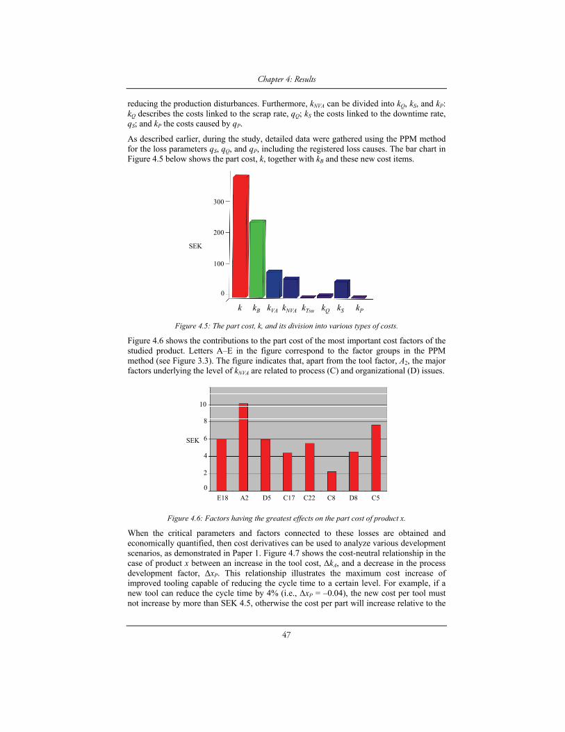
Chapter 4: Results

47

reducing the production disturbances. Furthermore, kNVA can be divided into kQ, kS, and kP: kQ describes the costs linked to the scrap rate, qQ; kS the costs linked to the downtime rate, qS; and kP the costs caused by qP.

As described earlier, during the study, detailed data were gathered using the PPM method for the loss parameters qS, qQ, and qP, including the registered loss causes. The bar chart in Figure 4.5 below shows the part cost, k, together with kB and these new cost items.

Figure 4.5: The part cost, k, and its division into various types of costs.

Figure 4.6 shows the contributions to the part cost of the most important cost factors of the studied product. Letters A–E in the figure correspond to the factor groups in the PPM method (see Figure 3.3). The figure indicates that, apart from the tool factor, A2, the major factors underlying the level of kNVA are related to process (C) and organizational (D) issues.

Figure 4.6: Factors having the greatest effects on the part cost of product x.

When the critical parameters and factors connected to these losses are obtained and economically quantified, then cost derivatives can be used to analyze various development scenarios, as demonstrated in Paper 1. Figure 4.7 shows the cost-neutral relationship in the case of product x between an increase in the tool cost, ΔkA, and a decrease in the process development factor, ΔxP. This relationship illustrates the maximum cost increase of improved tooling capable of reducing the cycle time to a certain level. For example, if a new tool can reduce the cycle time by 4% (i.e., ΔxP = –0.04), the new cost per tool must not increase by more than SEK 4.5, otherwise the cost per part will increase relative to the

SEK

k kB kVA kNVA kTsu kQ kS kP

200

300

100

0

E18 A2 D5 C17 C22 C8 D8 C5

10

8

6

4

2

0

SEK

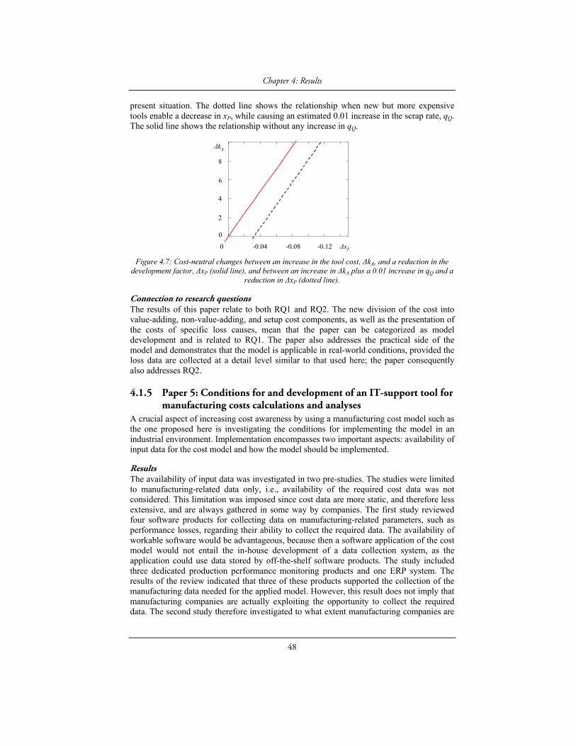
Chapter 4: Results

48

present situation. The dotted line shows the relationship when new but more expensive tools enable a decrease in xP, while causing an estimated 0.01 increase in the scrap rate, qQ. The solid line shows the relationship without any increase in qQ.

Figure 4.7: Cost-neutral changes between an increase in the tool cost, ΔkA, and a reduction in the development factor, ΔxP (solid line), and between an increase in ΔkA plus a 0.01 increase in qQ and a

reduction in ΔxP (dotted line).

Connection to research questions The results of this paper relate to both RQ1 and RQ2. The new division of the cost into value-adding, non-value-adding, and setup cost components, as well as the presentation of the costs of specific loss causes, mean that the paper can be categorized as model development and is related to RQ1. The paper also addresses the practical side of the model and demonstrates that the model is applicable in real-world conditions, provided the loss data are collected at a detail level similar to that used here; the paper consequently also addresses RQ2.

4.1.5 Paper 5: Conditions for and development of an IT-support tool for manufacturing costs calculations and analyses

A crucial aspect of increasing cost awareness by using a manufacturing cost model such as the one proposed here is investigating the conditions for implementing the model in an industrial environment. Implementation encompasses two important aspects: availability of input data for the cost model and how the model should be implemented.

Results The availability of input data was investigated in two pre-studies. The studies were limited to manufacturing-related data only, i.e., availability of the required cost data was not considered. This limitation was imposed since cost data are more static, and therefore less extensive, and are always gathered in some way by companies. The first study reviewed four software products for collecting data on manufacturing-related parameters, such as performance losses, regarding their ability to collect the required data. The availability of workable software would be advantageous, because then a software application of the cost model would not entail the in-house development of a data collection system, as the application could use data stored by off-the-shelf software products. The study included three dedicated production performance monitoring products and one ERP system. The results of the review indicated that three of these products supported the collection of the manufacturing data needed for the applied model. However, this result does not imply that manufacturing companies are actually exploiting the opportunity to collect the required data. The second study therefore investigated to what extent manufacturing companies are

0

0 -0.04 -0.08 -0.12

0

8

6

4

2

ΔxP

ΔkA

Chapter 4: Results

49

collecting the required data. This study demonstrated that, although the manufacturing companies participating in the study were largely able to collect the needed data, none of them were collecting all the required data.

Based on the results of the pre-studies, it was decided to develop a software application of the cost model jointly with a typical intended application user. The input data for the software should be based on data the company has already collected for other purposes. Before the application was developed, a list of criteria was established that the application had to fulfill, as follows:

to indicate the cost of every completed order number in cost per part to indicate the cost distribution between material, value-added, non-value-added,

and support activities to indicate the cost distribution between various non-value-added activities to visualize the results accessibly to provide a user-friendly interface to permit “what-if” analyses, i.e., analyses of how the cost is affected by various

changes in parameter values

Based on these criteria, the application was initially divided into two sheets, i.e., Part cost and What-if, but the final version of the application contained two more sheets, i.e., Batch cost and Process cost. Each sheet contains various tables and charts and a menu in which the user can select the products analyzed and the applicable time horizon. Figure 4.8 shows a screen shot of the part cost sheet.

Figure 4.8: Screen shot of the part cost sheet in the cost software.

The purpose of the part cost sheet is to display various calculations linked to the cost per part, k. The sheet includes tables and charts showing the cumulative cost per part from raw material to finished part. Information is also available regarding the values of the underlying parameters on which the part cost calculations are based. Figure 4.9 shows an example of a chart available in this sheet. The chart shows the increase in part cost contributed by every processing step, divided into value-added and non-value-added costs.

Chapter 4: Results

50

Figure 4.9: The cumulative costs at each processing step, divided into value-added costs and various non-value-added costs.

The batch cost sheet presents the total manufacturing costs of a batch, i.e., part cost multiplied by batch size. The process cost sheet presents the costs linked to machines and machine groups instead of to manufactured parts, indicating where in the plant the costs occur as well as the size of the costs. Figure 4.10 shows a bar chart from the process cost sheet showing the cost per hour of various machine groups.

Figure 4.10: Process cost per hour for various machine groups; each bar represents a machine group.

The purpose of the what-if sheet is to make simple simulations that indicate how the cost is affected by changes in input parameter values. The sheet shows the actual part costs and the values of the parameters on which these costs are based, just as in the part cost sheet. The difference is that this sheet also contains input fields in which one can enter new values for the parameters contained in the cost model and examine how the new values alter the part costs.

Connection to research questions This paper addresses both RQ1 and RQ2. The process cost equations represent model development and thus answer RQ1. The investigations of the industrial conditions necessary for the model and the development of the software prototype represent answers to RQ2.

4.1.6 Paper 6: Availability improvement by structured data collection: a study at a sawmill

This paper explores the role of availability monitoring as a tool for gaining knowledge of availability losses. The purpose is to investigate, first, whether an increase in the detail level of the collected downtime loss data improves the knowledge of what corrective action to implement and, second, how the personnel responsible for reporting the availability losses perceive the increased detail.

Utilization cost

Setup cost

Downtime cost

Value-added cost

Scrap cost

Cumulative cost

Utilization cost

Setup cost

Downtime cost

Value-added cost

Scrap cost

Chapter 4: Results

51

Results The study was carried out in a sawmill company. The company had a system that automatically registered downtime durations, but the operators still needed to choose an appropriate downtime cause from a list available in the system. To investigate how more detailed monitoring affected the knowledge gained, a new list of downtime causes was created, including a new list structure grouping the causes. The original list represented essentially all types of equipment, but only a few downtime cause alternatives were offered for each piece of equipment. The production manager also believed that some downtime causes were missing from the system’s lists. There was some dissatisfaction with the list structure, for example, setup time and unplanned tool exchange were found in the same downtime group. A total of 128 downtime causes were available in the system before the implemented changes.

The changes in the downtime monitoring system started with the structure of the downtime cause list. The new structure, based on PPM concept developed by Ståhl [17] (see section 3.1.2.1), is more consistent than the previous one. Now every piece of equipment has essentially the same categories of downtime causes, comprising Tools (only for the equipment incorporating tools), Material, and four machine-related categories. A division was made between processing and material-handling equipment, the former having a more detailed set of downtime causes than the latter. Figure 4.11 shows an example of how the new tree structure of the downtime causes is structured, in which the group Saw group 1 and its material handling equipment is expanded.

Chapter 4: Results

52

Figure 4.11: Example of the new structure and list of downtime causes.

As mentioned above, the list of downtime causes for the processing equipment has a more detailed structure then the list for the material handling devices. The latter offers only six downtime causes to choose from, as shown in the lower box in Figure 4.11, and they are the same for every piece of material handling equipment. For the processing equipment, the Tools and Material subgroups include specific downtime items for every machine, the other causes (indicated by the large rectangle in the figure) reappearing for every piece of processing equipment. Maintenance-related downtimes consume maintenance resources, so it is useful to highlight and separate them from the other downtimes. It was also decided that preventive and corrective maintenance should be separated, making it possible, for example, to investigate how increases in preventive maintenance affect the amount of corrective maintenance needed. These changes resulted in a downtime monitoring system now containing 292 individual downtime causes.

Level 1

Saw group 1 and its material handling equipment

Saw group 1

Intake

Outtake

Board transport

Tools

Material

Machine - Electrical

Machine - Mechanical

Machine - Computer

Hook sawingStone sawing

Band breakdownReducer toolChange of bladeUnknown/other

Broken logHooked logWrong timber class

MisadjustedUnplanned – Fixed by operatorsPreventive maintenanceCorrective maintenance

MisadjustedUnplanned – Fixed by operators

Preventive maintenanceCorrective maintenance

MisadjustedUnplanned – Fixed by operatorsPreventive maintenanceCorrective maintenance

Log pusher Saw group 1

Material

Machine - ElectricalMachine - MechanicalMachine - Computer

Machine - Unknown/other

Machine - Lack of education

Machine - Unknown/otherMachine - Lack of education

The same for every piece of processing equipment

Equipment-specific causes

Level 2 Level 3 Level 4

The same for every piece of material handling equipment

Unknown/other

Log intake

Edgers

Transporters -lower floor

Green sorting - Boards

Setup

Miscellaneous



Band crack

Green sorting - Planks

Chapter 4: Results

53

One question addressed in the paper was whether an increase in the level of detail regarding the specification of downtime causes could improve a company’s knowledge of its availability losses. According to the production manager, the changes in the downtime system have improved the usability of the collected data. The data now indicate more precisely what has happened and therefore what needs to be done to improve the situation. Because of the higher level of detail in the list of available downtime causes, the production manager now finds it easier to steer discussions with operators toward specific problems.

The other question raised in the paper was how the personnel responsible for reporting the availability losses perceive the increased level of detail. The interviews with the operators indicated that they generally favored the new list of downtime causes. The new list enables them to choose a downtime cause that actually describes the occurred stoppage, making the monitoring more precise. With more downtime causes to choose from, the operators might feel that the data collection is overly complicated and time-consuming; however, the interview results indicated that they generally did not feel that the new system included too many downtime causes, and that they appreciated the possibility of selecting more correct downtime causes.

Connection to research questions This paper takes one step backward and addresses the collection of input data for the cost model. Paper 4 demonstrated that the cost model was applicable in an industrial context, provided the company collected data at a level of detail similar to that used in the study. Paper 5 further investigated the conditions for the industrial use of the cost model and demonstrated that existing software products could support the collection of the required data. Finally, Paper 6 demonstrated that the required level of input data detail was manageable under real-world conditions; the paper thus addresses the conditions for industrial use and consequently answers RQ2.

Chapter 4: Results

54

4.2 Cost model – Clarifications and enhanced downtime and equipment cost calculations

The cost model originally published in Paper 1 has since been refined, most of the related changes having been included in papers 2–5. However, some of the refinements were not covered in the appended papers; those will be presented here, together with a more general formulation of the cost model than the one published in Paper 1. The general formulation clarifies that the model describes any processing step in a product’s processing chain by formulating the equations in a more general way by using the index i, which describes the processing step. The index had already been introduced in papers 3 and 5, but not in all of the equations pertaining to the model.

In the original model presented in Paper 1, the batch size, N0, describes the nominal batch size, i.e., the ideal number of parts produced in a scenario in which no scrapping occurs. If scrapping does occur, additional parts must be produced to meet customer demands, resulting in the real batch size, N. This formulation of the batch size describes a situation in which the final batch size is not determined before order production starts; instead, it depends on the number of parts scrapped when manufacturing the order. Such a configuration can prevail in a make-to-order situation in which buffers and other types of part stockpiling are undesired. However, companies often adopt a strategy in which the initial batch size is fixed, not varying depending on whether or not scrapping occurs. The size of the batch arriving at a specific processing step then depends on the size of the batch when it left the previous step. This type of configuration is modeled in section 4.2.2.

The original model contains two parameters for equipment costs: kCP, the equipment cost rate during production, and kCS, the equipment cost rate during downtime and idle time. In Paper 1, these two parameters were described only briefly, but section 4.2.2.1 presents a more detailed formulation of kCP and kCS that takes into account the key parameters affecting these costs.

4.2.1 Main principle of the proposed cost model The focus of the proposed cost model is the influence of each processing step on the total cost of each part. It is a cost center approach in which the cost center comprises every freestanding processing step, i.e., processing steps separated by buffers, in the processing chain. Such a processing step is here referred to as a planning point. Every planning point is represented by a cost equation, which means that every planning point has a specific kCP, kCS, and kD together with the other parameters included in the cost model. A planning point can consist of several unique process steps, but these steps share a common nominal bottleneck station that determines the common nominal cycle time, t0, of the planning point. Figure 4.12 illustrates the cost center approach employed. The cost allocation is mainly time driven, which means that the shares of the total equipment and wage costs allocated to the parts are based on the length of time each part resides in each piece of equipment. This time is determined by times related to the equipment capacity, such as processing time and material handling time, and by disturbances causing breakdowns, small stoppages, or reduced production speed. The non-time-driven cost in the model consists of the cost of scrapped parts, which is taken into consideration by defining the part cost as the cost per correctly manufactured part. Hence the cost of the batch in a specific processing step is divided by the number of correctly manufactured parts.

The proposed approach makes it possible to describe how a part’s cumulative cost is built up by the processing steps it undergoes. It also makes it possible to determine to what

Chapter 4: Results

55

extent these costs are constituted by valued-adding activities and to what extent they are constituted by disturbances, such as downtimes and quality deviations. In addition, the distribution between material, equipment, and wage costs at every processing step can be visualized, illustrated by the bar charts and circle charts in Figure 4.12. Such presentations of the costs involved are intended to foster understanding of how different economic and manufacturing technology-related parameters affect the cost of parts produced in a manufacturing system.

Figure 4.12: (a) The cost center approach and examples of possible analyses. (b) Bar charts showing the added cost associated with a specific processing step. (c) The share of material, VA, NVA, and NNVA costs in each processing step. (d) The cumulative shares of material, equipment, and wage

costs.

4.2.2 Modeling the part cost The nominal processing time (cycle time), t0, in processing step i for a part comprises machine time, tm, handling time, th, and tool change time, tvb, according to Equation 4.17.

Cost per part

Cost from previous step

VA cost

NVA and NNVA

Material cost (b)

(c)

(d)

NVA cost

NNVA cost

VA cost

Material cost

Wage cost Equipment cost

Planning point no 1

TimesLossesCosts

Planning point no 2

TimesLossesCosts

Planning point no 3

TimesLossesCosts

(a)

Chapter 4: Results

56

iiii vbhm0 tttt 4.17

In the original version of the cost model, the downtime rate, qS, included all planned and unplanned downtime except for setup time and utilization losses. Implementations of the model have revealed the deficiencies of such an approach when it comes to calculating the cost of a specific batch. This is because planned downtime normally often occurs between batches, as illustrated in Figure 4.13, so there is no specific batch to which to logically allocate it. A more logical way to handle planned downtime is to allocate its costs not to the parts produced in a specific batch, but to all produced products in relation to the length of each batch time, i.e., according to the same principle as used for machine utilization losses, URP (see Equation 4.5). This results in the planned downtime being distributed uniformly as an extra cost per unit time during production, unplanned downtime, and setup time.

Figure 4.13: Illustrative timeline of hypothetical manufacturing equipment.

Allocating planned downtime costs in a way similar to the allocation of utilization losses costs is logical, because utilization losses are actually a type of planned downtime. Although setup time (Tsu) is also a planned downtime, the definition of Tsu will remain unchanged, because setup times are clearly connected to specific batches.

Clearly distinguishing between planned and unplanned downtime is also sound in the sense that there are clear differences between their causes: the former are organizationally related, scheduled by the company, and sometimes carried out to reduce the latter.

As a result of these changes, the downtime rate will be divided into two main types: the planned downtime rate, qS1, and the unplanned downtime rate, qS2. The formulations of these rates, as well as the scrap rate, qQ, and production-rate loss, qP, are presented in Figure 4.14, where the rates are calculated by dividing the loss time (indicated in the red square) by the time in the blue rectangle above it. Compared to the OEE performance parameters (i.e., A, O, and P), qP is equivalent to 1 – P and qQ is equivalent to 1 – Q; qS2 is equivalent to 1 – A, except that qS2 does not include setup time.

Setup time

Production time

Unplanned downtime

Planned downtime (planned maintenance, other)

Batch 1 Batch 2 Batch 3 Batch 4

Utilization losses

Theoretical production time, Ttheo

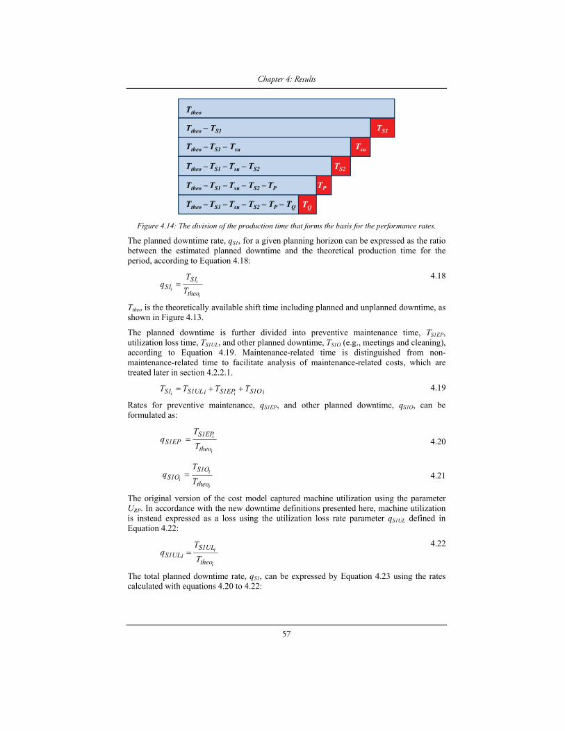
Chapter 4: Results

57

Figure 4.14: The division of the production time that forms the basis for the performance rates.

The planned downtime rate, qS1, for a given planning horizon can be expressed as the ratio between the estimated planned downtime and the theoretical production time for the period, according to Equation 4.18:

i

i

itheo

S1S1 T

Tq

4.18

Ttheo is the theoretically available shift time including planned and unplanned downtime, as shown in Figure 4.13.

The planned downtime is further divided into preventive maintenance time, TS1EP, utilization loss time, TS1UL, and other planned downtime, TS1O (e.g., meetings and cleaning), according to Equation 4.19. Maintenance-related time is distinguished from non-maintenance-related time to facilitate analysis of maintenance-related costs, which are treated later in section 4.2.2.1.

iS1OS1EPiS1ULS1 TTTTii 4.19

Rates for preventive maintenance, qS1EP, and other planned downtime, qS1O, can be formulated as:

i

i

theo

S1EPS1EP T

Tq 4.20

i

i

itheo

S1OS1O T

Tq 4.21

The original version of the cost model captured machine utilization using the parameter URP. In accordance with the new downtime definitions presented here, machine utilization is instead expressed as a loss using the utilization loss rate parameter qS1UL defined in Equation 4.22:

i

i

theo

S1ULiS1UL T

Tq

4.22

The total planned downtime rate, qS1, can be expressed by Equation 4.23 using the rates calculated with equations 4.20 to 4.22:

TS1

Tsu

TS2

TQ

TP

Ttheo

Ttheo – TS1

Ttheo – TS1 – Tsu

Ttheo – TS1 – Tsu – TS2

Ttheo – TS1 – Tsu – TS2 – TP

Ttheo – TS1 – Tsu – TS2 – TP – TQ

Chapter 4: Results

58

iS1OS1EPiS1ULiS1 qqqqi 4.23

As stated earlier, the planned downtime is allocated to a batch in relation to the total time needed to manufacture a batch. The planned downtime allocated to a batch, TS1b, is defined in Equation 4.24:

ii

i S1S1

ibS1b q

q

TT

1

4.24

The mean unplanned downtime rate, qS2, for a planning horizon is defined as the ratio between total unplanned downtime, TS2, and the theoretical production time minus the planned downtime and setup time for the period, according to Equation 4.25:

iii

suiS1theo

iS2S2 TTT

Tq

4.25

According to the same principle as used for planned downtime, the total unplanned downtime, TS2, is divided into time for corrective maintenance, TS2EC, and other unplanned downtime, TS2O, according to Equation 4.26:

iOSECSiS2 TTTi 22 4.26

The corrective maintenance rate, qS2EC, and the downtime rate for other unplanned downtime, qS2O, are defined by equations 4.27 and 4.28:

ii

i

isuiS1theo

S2ECS2EC TTT

Tq

4.27

ii

i

suiS1theo

S2OiS2O TTT

Tq

4.28

Production-rate loss, qP, denotes speed losses due to short stoppages and increased cycle times. Equation 4.29 represents qP, where TP is the production-rate loss time:

iii

i

isuS2iS1theo

PP TTTT

Tq

4.29

Equation 4.30 expresses the scrap rate, qQ, where NQ is the number of scrapped parts in processing step i and Ni is the batch size for processing step i, excluding scrapped parts, i.e., the number of correctly manufactured units. The scrap rate, qQ, can also be expressed in terms of time according to Equation 4.31, where TQ is the nominal production time for the scrapped parts:

1

1

1

i

ii

i

QQ N

NN

N

Nq i

i

4.30

iiiii

PsuS2S1itheo

iQQ TTTTT

Tq

4.31

The production time for a batch, Tb, can be expressed in two ways depending on whether or not Tb is affected by the scrap rate, qQ. In make-to-order situations in which specific quantities of correct units must be produced, Tb will be dependent on qQ because additional

Chapter 4: Results

59

parts must be produced, according to Equation 4.32. On the other hand, in a make-to-stock situation, the production time, Tb, will not be affected by qQ, according to Equation 4.33:

)1()1()1(

1

iii

i

iiPS2Q

0isub qqq

tNTT

4.32

)1()1(

1

ii

i

iiPS2

0isub qq

tNTT

4.33

The cost per part is defined according to Equation 4.34. There are several differences between this part cost equation and the one found in Paper 1 (Equation 4.9). Equation 4.34 expresses the cost per part more generally by introducing the processing step index, i. It also includes greater detail due to the modified downtime rates described above, and includes rows describing the costs of tools and corrective maintenance (these two costs are described in section 4.2.2.1).

ES2

S2EC

PQ

0EC

DQi

S1bsu

PS2Q

0D

CQi

S1bsu

S2

S2

PQ

0CS

CPQ

0CP

AiPQ

mA

Q

ii

i

i

ii

ii

i

ii

iii

ii

i

ii

i

i

ii

ii

ii

ii

i

i

ii

q

q

qq

tk

qN

TT

qqq

tk

qN

TT

q

q

qq

tk

qq

tk

qq

tk

q

kk

)1()1()1(60

)1()1()1()1(60

)1()1()1()1(60

)1()1(60

)1()1(601

1

1

1

4.34

The first expression in Equation 4.34 describes the value of a part as it enters processing step i and the extra cost resulting from scrapped parts. The cost of a part as it enters the first processing step consists of the material cost, including the raw material and indirect material costs, and is denoted kB. Equation 4.34 is formulated for an arbitrary production step, which means that if i = 1, then ki–1 =kB. Indexes A–E in the cost model relate to different groups of causes in the production performance matrix, described in section 3.1.2.1, i.e., A is tool related, B material related, C machine related, etc. Bracket A describes the tool cost, which is defined in section 4.2.2.1. The first C bracket expresses the machine cost during the operating time per correctly manufactured part, and the second C bracket describes the total downtime cost per correct part. Bracket D includes the wage cost per correctly manufactured part; kD is the wage cost per hour, including social insurance expenditure and other labor taxes, the hourly rate being calculated based on theoretical production time. Only what is traditionally classified as direct labor is included in kD, i.e., personnel directly connected to the production process, such as machine operators. The wage cost per correctly manufactured part is a function of the total production time including setup time. Bracket E describes the cost of corrective maintenance.

Chapter 4: Results

60

4.2.2.1 Equipment costs Here follows more detailed formulations of the equipment cost parameters kCP and kCS than are found in Paper 1. The equipment cost, which sometimes constitutes much of the manufacturing cost, can be calculated in numerous ways. This leads to the conclusion that the equipment cost must be defined at a higher level of detail than other costs, yielding a precise definition appropriate for the analyses for which the cost model is to be used.

Depreciation and interest costs All the manufacturing cost models examined in the literature review that include the investment cost of equipment consider only the depreciation cost and sometimes also the installation cost. None of them consider the interest cost—or cost of capital, as it is usually called. Why this cost is neglected is unclear, though it is possibly because there are different opinions as to whether the cost of capital should be regarded as a cost in product costing and equipment cost calculations [39]. For a company applying interest costs in its calculations, a suitable approach for the present cost model is to use the capital recovery factor. This factor results in an evenly distributed yearly cost, enabling fair and convenient comparison of the cost effects of equipment of various ages, independent of how long the equipment has been used. For the same reason, it is recommended that the hourly cost be based on the useful life of the equipment, instead of using a fixed depreciation period. Groover [104] also uses the capital recovery factor in equipment cost calculations; unlike Groover’s model, the proposed cost equations include more detailed descriptions of the costs included in the machine cost, instead of using the overhead rate used by Groover.

The initial investment expense is denoted I0 and also includes, in addition to the investment cost, the costs of equipment installation. The yearly cost of the initial investment, the annuity, is denoted a and the interest rate r. The interest rate should reflect the company’s cost of financing the investment. Equation 4.35 defines the annuity, a, where n is the estimated economically useful life of the machine:

1)1(

)1(

n

n

0r

rrIa

4.35

Floor space cost The equipment occupies a specific floor area, F, in the factory building. The building is associated with certain costs, such as the depreciation, utilities, and maintenance costs, that can be formulated as a cost per square meter, kCF. The product of F and kCF therefore represents the floor area cost of the equipment. This is a standard calculation found, for example, in Son [76].

Cost of preventive maintenance Preventive maintenance is a planned periodic activity resulting in a periodic cost, normally occurring after a specific number of operating hours. Converting this to a cost not varying in time depending on the specific occurrence of maintenance tasks distributes the costs evenly over the operating time. The preventive maintenance cost per hour is denoted kEP and consists of the labor costs for maintenance personnel and other maintenance department costs, such as the costs of equipment and the computer system for maintenance activity documentation. kEP can be derived by calculating the total cost of the maintenance department, KE, over the planning horizon, divided by the department’s total practical capacity (i.e., number of employees in the maintenance department, nEavail, multiplied by the practical capacity per employee, TEavail). This rate is then multiplied by nEused, which is

Chapter 4: Results

61

the average number of workers performing a preventive maintenance task. As shown in equations 4.38 and 4.39, kEP is multiplied by TS1EP, which is the estimated preventive maintenance time for the planning horizon.

60Eavail

Eavail

iEusedEEP T

n

nKk

i

4.36

The corrective maintenance cost is described separately in the part cost model, and is not included in the equipment cost parameters.

Variable costs Equipment operation is associated with energy consumption and often with additives such as cutting fluids and lubricants. These variable costs are denoted kV, which is defined in Equation 4.37; kep is the hourly energy cost of the equipment during production and kadd is the total cost of additives per hour. How easy these costs are to determine depends on how they are documented and structured by the company. The energy cost per hour can be calculated by measuring the energy consumption of the machines and multiplying the consumption by the energy cost rate. If these cost items cannot be obtained directly, they can be estimated.

iii epaddV kkk 4.37

Hourly equipment costs The part cost model presented earlier in this thesis separates the total equipment cost into the cost of equipment during operation and during downtime (e.g., setup and unplanned downtime). Therefore, two machine cost rates are formulated, one for the cost during operation, kCP, and the other for the cost during downtime, kCS. To calculate the hourly machine cost, the previously noted cost items are divided by the yearly theoretical production time, Ttheo. Equation 4.38 expresses the hourly machine cost during production, kCP.

iVtheo

S1EPEPCFii

CP kT

TkkFa

ki

i

ii

i

60

60

4.38

The hourly machine cost during downtime, kCS, is calculated by reducing the machine cost during production, kCP, by the variable machine costs included in kV. Machines may consume energy even during downtime, when they may be in standby mode, and this energy consumption is denoted kes.

ii

i

ii

i estheo

S1EPEPCFii

CS kT

TkkFa

k

60

60

4.39

Cost of corrective maintenance The cost of corrective maintenance is not included in the machine cost expressions, but is instead described separately in Equation 4.34. The cost of corrective maintenance is not included in the hourly machine cost expressions because the corrective maintenance cost is

Chapter 4: Results

62

viewed as a special type of downtime cost, not an equipment cost. The corrective maintenance cost per hour is denoted kEC and can be derived in the same way as can the hourly cost of preventive maintenance, as described in Equation 4.36. This cost is multiplied by the corrective maintenance time per part using qS2EC. The expression for the corrective maintenance cost per correct part, kec, is described in Equation 4.40:

)1()1()1(60i

i

ii

ii

iS2

S2EC

PQ

0ECec q

q

qq

tkk

4.40

Tool cost A tool or tool system can have different characteristics depending on the type of machine involved. Many types of machines, such as lathes and milling machines, have a tool system consisting of a tool holder and an insert. The cost models of Cauchick-Miguel and Coppini [71] and Branker et al. [78], for example, are based on such a system. The formulation of the tool cost per hour in this thesis is based on the same system, and is shown in Equation 4.41. In this approach, kth is the tool holder cost, which is divided by Tth, the estimated tool holder life; kt is the cost per insert and Tt the insert life. If the insert consists of more than one cutting edge, the parameter nt, which describes the number of edges, can be applied. Unlike the tool cost as formulated in Cauchick-Miguel and Coppini [71] and Branker et al. [78], Equation 4.41 includes an expression for overhead costs related to the tools, ktOH, which can include the costs of tool sharpening. ktOH is multiplied by the estimated time spent on these activities over a planning horizon, TtOHused, and then divided by the time available over the same planning horizon, TtOHavail. The hourly costs are multiplied by the machine processing time, tm, to obtain the cost per part. In addition to scrapped parts, speed losses resulting from increased tm can be taken into account by qP, but only the share of qP resulting from increased tm and not short stoppages that can also be included in the qP parameter.

60

60

6060

tOHavail

tOHusedtOH

tt

t

th

thA T

Tk

Tn

k

T

kk

i

i

i

i

i

i

i

4.41

4.2.3 Connection to research questions Since the publication of Paper 1, it has been realized that the equipment cost needed to be defined in greater detail, because it can constitute a significant part of the total manufacturing cost in some manufacturing systems, for example, highly automated manufacturing systems. The equipment cost equations presented here can be regarded as a supplement to Paper 1, added to make the cost model more comprehensive, and thus address RQ1. As a result, the model now includes more parameters of interest when analyzing manufacturing cost issues, for example, the relationship between preventive maintenance and unplanned downtime. The other modifications of the cost model introduced in section 4.2.2, for example, the division of the downtime rate into planned and unplanned downtime rates, also address RQ1 and were made so the model would be more applicable. The cost allocation is now more logical, since planned downtime is now distributed evenly over the production time. The introduction of the new downtime parameters describing the rates of preventive and corrective maintenance enables analysis of the impacts of different types of maintenance activities. In addition, the cost model now takes into account the fact that unplanned downtime, the correction of which requires

Chapter 4: Results

63

formal maintenance resources, is more costly than downtime handled by the operators themselves.

Chapter 5: Discussion

64

5 Discussion This chapter relates the results of the thesis to the literature findings presented in chapter 3. In particular, the cost model is compared with the cost accounting methods described in section 3.2 and with the cost models described in section 3.3.

Companies today use alternative methods to measure their manufacturing performance and to calculate costs related to the manufacturing department and other departments. One popular method for measuring manufacturing performance is OEE. OEE includes many of the parameters found in the proposed model and can be used to address similar issues, for example, how equipment is performing and the distribution of losses between scrap, downtime, and production-rate losses. However, because OEE does not include cost considerations, it cannot provide the same insight into performance as can the proposed model. For example, the definition of OEE results in a 5% quality-rate loss having the same impact on the OEE figures as a 5% downtime-rate loss. OEE consequently neglects the material cost, the value accumulated after each processing step, and the cost rate of the processing step in which scrapping occurred. By expressing performance losses in terms of costs according to the proposed model, improvement activities can be prioritized more accurately than by using OEE.

At the beginning of the literature review, several theories of manufacturing system performance were presented, including the sand cone model. This model claims that improvement work must be conducted in a specific sequence, starting with quality, then dependability, speed, and finally cost, to avoid tradeoffs. Whether or not the sand cone theory is true is debatable, but at least the sequence of the first three layers in the sand cone feels intuitively sound. The fourth layer, i.e., cost, is not necessarily wrong, but the present author believes that cost reduction should not be a final, isolated activity, because, according to the proposed model, costs are linked to the first three layers in the sand cone model. Improvement in quality, for example, may initially entail an investment cost, but the improved quality rate can result in an overall cost reduction per part. Furthermore, reducing the manufacturing cost calls for improvements of some sort, and these improvements may include improvements in quality, dependability, or speed. The cost layer can therefore be regarded as interrelated with the other three layers.

The theory of performance frontiers proposed by Schmenner and Swink [22], partly based on the sand cone model, is interesting in relation to the present work. The asset frontier, describing the frontier determined by equipment, is the maximum performance possible using the equipment in a manufacturing system. Using the proposed model, the asset frontier is equivalent to a situation in which qQ, qP, qS1, qS2, and Tsu must be 0 in the bottleneck process and probably near 0 in other processes in order to minimize the number of operators and the quantity of required maintenance resources. The operating frontier is more difficult to define in general terms. According to Schmenner and Swink [22], the operating frontier is determined by present operating policies; if the company is at this frontier, then performance improvement will result in increased cost, i.e., improving qQ, qP, qS1, qS2, or Tsu will increase the part cost. If the company is somewhere to the left of its operating frontier, then improving qQ, qP, qS1, qS2, or Tsu will lead to a lower or unchanged part cost. This theory can be useful when applied together with the proposed cost model, as it can help explain situations in which improving any of the performance parameters of the model increases the part cost. If the parameters are not close to their optimal values, then the company should consider changes in the operating procedure instead of investing in new equipment.


65

5.1 The proposed cost model in relation to general cost accounting methods

In this section, the proposed cost model (here referred to as “model A”) will be described in relation to the methods presented in section 3.2, namely, traditional cost accounting, activity-based costing (ABC), time-driven activity-based costing (TDABC), throughput accounting (TA), life cycle costing (LCC), kaizen costing, and resource consumption accounting (RCA). The purpose of the comparison is to indentify similarities and differences in terms of purpose, principle, and cost allocation.

Purpose The purpose of model A is to support decisions regarding improvement activities in manufacturing systems. The model should describe the cost impacts of current manufacturing conditions and of planned decisions. This is realized by including only costs and other parameters affected by decisions made in the manufacturing department. It is a cost concept intended to be used by personnel in the manufacturing department of a company, to raise the cost consciousness of manufacturing personnel. Its focus on manufacturing costs distinguishes the concept from traditional cost accounting, ABC, TDABC, and RCA, all of which are cost accounting concepts applicable to whole organizations and all types of businesses. LCC can also be used in many types of businesses, but its focus is on the costs associated with the buying/making, owning, and disposal of a product, which distinguishes it from the just-mentioned methods and from model A.

TA has a clearer manufacturing focus than do the other mentioned methods. Its focus is on throughput and constraints, for example, a bottleneck station in a manufacturing line, and it is intended to maximize the return in the bottleneck or maximize the relationship between the profit and cost rates of a product. TA is consequently used for bottleneck analysis and profit maximizing, which distinguishes it from model A’s focus on the connection between performance and costs in every processing step. However, the impact of the bottleneck station is not neglected, because it affects the cycle time, t0, in the model. Another major difference between model A and TA is that TA includes revenues and not only costs.

Model A and kaizen costing are also somewhat similar in purpose. Kaizen costing is about cost reduction in the manufacturing phase of a product. Specific cost reduction targets are determined for the whole plant, and these targets are then distributed to specific plant processes. Two similarities are the cost reduction focus and the connection between costs and manufacturing performance. However, there are also important differences. Kaizen costing is largely a top–down approach in which cost reduction targets are determined by top management. It is then the responsibility of the managers in the manufacturing departments to ensure that these targets are realized. Another difference is that the purpose of model A is not solely to support cost reduction, but also to support cost-conscious manufacturing generally, to learn how various manufacturing system parameters affect the manufacturing cost.

Principle Model A is based on processing steps, each of which is a cost pool. A process drives a specific number of costs due to equipment depreciation, operator wages, energy consumption, etc. These costs are allocated to a manufactured part based on the time needed to process it in the specific step; only costs impinging directly on the processes are included. The purpose of this structure is related to the purpose of the concept itself: the


66

costs of a part in every processing step are made clear in order to learn how the manufacturing costs accumulate as the part undergoes various process steps. In addition to the cycle time, equipment, and wage costs, there may also be non-value-added activities and setup time linked to a process step that add to the cost per part. Section 4.2.1 describes the main principle of model A.

Of the methods included in this comparison, RCA and TDABC are the most similar to model A in terms of the main principle. In RCA, costs are allocated to so-called resource pools, linked to each other based on the cost flow. A resource pool can be a process step in a manufacturing plant, but it can also be a department or another resource group. Like model A, RCA is a time-driven method, even if activities can also be applied as in ABC. RCA differs from model A in that it is a general method lacking, for example, the loss parameters included in model A. TDABC is also based on process steps, and it is time driven, based on the cycle time, as is model A. Like RCA, it is a general model and hence does not include production parameters other than cycle time.

Cost allocation Because the aim of model A is to connect manufacturing parameters to costs, it was considered important when developing the model to establish logical cost allocations to the cost pools and manufactured parts and thus avoid arbitrary allocations. As with TDABC and RCA, implementing model A takes advantage of the company’s ERP and MES systems and other systems the company uses to store data regarding cycle times, equipment performance, costs, maintenance activities, machine utilization, etc. Model A is highly dependent on the IT systems and data available at the company, meaning that the rationality and accuracy of the cost allocation are dependent on these systems. The basic principle of model A, that every process step is a cost pool, makes accurate allocation of the depreciation costs fairly straightforward if the company has specified depreciation costs for all equipment. Other costs related to the equipment, such as maintenance costs, can be more difficult to handle. Maintenance work can be divided into preventive and corrective maintenance. Correct allocation of these costs requires documentation of the quantity of resources and time spent on every cost pool, ideally separating preventive and corrective maintenance.

Energy costs can be divided into fixed and variable costs, the former including the costs of heating the production facilities and the latter the energy consumed by the manufacturing equipment. Because of increasing environmental awareness, companies are becoming more aware of their energy consumption, leading to better allocation of these costs. The energy consumption rate of equipment can be accurately derived using measurement devices. An alternative but slightly less accurate method is to use the energy consumption specified by the equipment supplier. If the fixed energy consumption is not directly available, an estimate may be made. The fixed costs are then allocated to the cost pools based on the occupied area.

In the past, when manufacturing plants were less automated, it was common for one operator to be assigned to each machine. Nowadays, it is not uncommon for one or a group of operators to be responsible for several machines simultaneously, becoming more of an overhead cost, like a support function. In such cases, operator cost can be allocated to the cost pools based on the estimated shares of time the operators or operator groups spend in specific cost pools.

The allocation principles used in model A are similar to those used in two of the most recently developed cost accounting methods, TDABC and RCA. As described above, these methods are based partly on the idea that companies today have considerable data stored in


67

various systems that can be useful in cost accounting. In TDABC, the cost pools are operating departments, or individual processes if the various processes in a department differ significantly in cost. Resources that cannot be directly linked to cost pools should be allocated to cost pools based on rational, cause–effect relationships. These allocations can be made using the same procedure as used to formulate the operation cost rates, i.e., using time equations. The cost of a support department, for example, can be allocated to operating departments by identifying the tasks carried out in the support department and their corresponding “cycle times.” The operating departments’ demands for these tasks are then quantified, resulting in causal relationships between the departments. This procedure is largely the same as the one used in model A, for example, concerning maintenance costs. The allocation principle in RCA is essentially the same as in TDABC (and model A). Even this method emphasizes allocations based on rational and causal relationships, though preferably not activity based as in traditional ABC.

The second allocation, i.e., from the cost pools to the manufactured parts, is based mainly on time in model A, the exception being the scrap cost. The present author believes that time-based allocation based on the cycle times of individual parts is the most accurate allocation principle and is also feasible in today’s manufacturing, in which cycle times for all product types are usually available in the company’s ERP or MES system. However, this imposes data maintenance requirements, and nominal times must be updated when modifications in the manufacturing system affect these times. Furthermore, the downtime-rate and production-rate losses must be available, preferably product-specific rates (except for the planned downtime-rate loss). The scrap cost is allocated to the manufactured part level by means of the scrap rate, which is based on the number of scrapped parts in relation to total quantity of parts. The inclusion of the scrap rate means that the cost per part expression describes the cost per non-scrapped part.

In addition to the cycle time (including the unplanned downtime-rate and production-rate losses) and scrap rate, a third allocation principle is used in model A. This principle is used to allocate the planned downtime cost down to manufactured parts, these costs being allocated based on the batch time. In the original version of the model, only the utilization losses were allocated based on this principle, but in the changes introduced into the model in section 4.2, all planned downtime is allocated to the parts in this way. The allocation procedure is similar to the one TDABC uses to allocate planned downtime, the differences being that the planned downtime is formulated as rates and that utilization losses are included. The formulations of the various downtime rates presented in section 4.2 emphasize the planned downtime, which is no longer hidden in the practical production time. In TDABC, as well as in ABC and RCA, the utilization losses are not treated in the same way as is the other planned downtime. The costs related to utilization losses are not allocated to cost objects, because this could lead to a downward spiral in which product prices are constantly increased to compensate for increased utilization loss costs, which in turn result from the reduced production volumes caused by higher prices. However, model A is not intended to be used for product pricing decisions, which makes the allocation of utilization loss costs suitable in this context.

This second allocation procedure in model A has clear similarities to the second allocation procedure in TDABC. TDABC advocates cycle-time-based allocation, although exceptions can be made if other allocation principles are more appropriate. Average cycle times are recommended; any losses in cycle time or losses due to scrapped parts are not considered. As just mentioned, the theory underlying TDABC also includes policies for handling unused capacity, which should be assigned to the person or unit responsible for its occurrence. For example, if idle capacity has occurred due to lower demands than expected


68

for a specific product, then the costs of the resulting idle capacity should be assigned to the person or organizational unit responsible for the product. The costs should not be allocated to individual products, because this could make some products appear unprofitable, leading to the downward spiral just mentioned.

The second allocation procedure in RCA is very similar to the one in TDABC. RCA theory advocates allocation based on quantitative causal relationships. It does not specifically recommend time, but because the theory also says that activity-based rates should be applied only in certain critical cases, it is assumed that time-based allocation is frequently used. In RCA, utilization losses are treated exactly as they are in TDABC, and for the same reasons.

5.1.1 Conclusions The comparison indicates that model A is somewhat similar to TA and kaizen costing in terms of purpose and focus, mainly because these are more manufacturing related than the other approaches. Kaizen costing is an interesting approach; the idea it uses of setting specific cost reduction targets is also mentioned in Paper 1 as a way of using the proposed model, described as deterministic production development, in contrast to the continuous development normally associated with lean production. Model A could indeed be used in a kaizen costing setting, as the model’s causal relationships between manufacturing parameters and costs could be used when determining cost reduction activities. As mentioned earlier, kaizen costing is used together with traditional cost accounting methods, and the method is more like the proposed model in practice than when making cost calculations.

The comparison also revealed similarities between model A and TDABC and RCA, for example, in their use of cost centers and time-driven costs. However, the latter two are more general methods applicable to any type of business and do not include any specific manufacturing-related parameters.

5.2 The proposed cost model in comparison with selected cost models

This section presents a comparison between the proposed cost model (model A) and five selected models described in section 3.3 (models B–F). The models included in the comparison are the models developed by Yamashina and Kubo (B) [75], Özbayrak et al. (C) [68], Son (D) [76], Chiadamrong (E) [77], and Dhavale (F) [70]. These models were chosen because they are more comprehensive models, as shown in the summary presented in Table 3.4. The comparison will relate the parameters and their definitions included in model A to the parameters and definitions in models B–F.

Main model purpose Model A: To support cost-conscious manufacturing; to describe the link between manufacturing technology, performance, and cost

Model B: To identify production losses to reduce costs

Model C: To estimate the difference in product cost between two planning systems, MRP and JIT

Model D: To estimate the manufacturing cost in advanced manufacturing systems

Model E: To calculate quality-related manufacturing costs


69

Model F: To calculate manufacturing costs in computer-integrated manufacturing systems

Material cost In model, A the material cost is the direct material cost for a specific product. Model B distinguishes between direct and indirect material costs (e.g., machining lubricant, a cost found in the variable equipment cost parameter of model A). Models D and E have similar approaches to that in B, but D also includes an ordering cost parameter. The material cost definition in models C and F is similar to that in A.

Equipment cost In the modified version of model A presented in section 4.2, the equipment cost includes the costs of depreciation, floor space, and preventive maintenance, as well as a variable cost describing extra costs during production, such as energy costs. Corrective maintenance is not included in the equipment cost parameters kCP and kCS, but is included in the model as a separate parameter. In addition, the tool cost is described separately. Section 4.2.2.1 describes the formulation of the equipment cost.

Model B does not have a specific equipment cost parameter, but includes cost items that can be considered equipment costs, i.e., depreciation, tool, die and jig, energy, and maintenance costs. How these costs should be calculated and what they more specifically include are unspecified.

Model C includes costs for the following resources that can be considered equipment related: machines and cutting tool holders, computer system, robot and AGV system, AS/RS system, fixed assets, externally provided resources (e.g., utility costs), cutting tools and fixtures, direct energy consumption, and other services (including maintenance). These costs are allocated to various activity cost centers, each consisting of a direct and an indirect cost pool. The indirect costs (e.g., externally provided resources) are distributed to the cost centers based on utilization levels obtained from simulation runs of the manufacturing system. In addition, the allocations from the cost centers to the products are based on simulations in which the percentage of the total time a product occupies a certain operation (i.e., activity center) determines the product’s share of the total operation cost. The depreciation cost is calculated based on the initial investment price and is formulated as an hourly rate based on the estimated useful life. The depreciation costs of the buildings are allocated to machines based on the floor space they occupy. Tool costs are allocated to the machines based on the number of tools consumed by each machine, assuming each tool has an average cutting life of 60 minutes.

Model D includes a machine cost comprising utility, maintenance, repair, insurance, and property tax costs. These costs are, except for property tax, formulated as hourly costs without any description of how these rates should be calculated. In addition, the model includes cost parameters for tool, floor space, and computer software costs. The tool cost is calculated as the cost per tool times the number of tools changed over a planning horizon. Depreciation costs are considered but no equation is formulated for it.

Model E includes a machine cost comprising utility costs and a material handling cost. The model also includes costs for preventive maintenance. Corrective maintenance is not directly mentioned, but it can be assumed that this is included in another parameter called “failure repairing cost.” Other equipment-related costs such as depreciation and tool costs are not considered because they are not regarded as affecting the cost of quality, which is the focus of this model.

Model F has no specific equipment cost item, but includes the following equipment-related costs: machine cost including depreciation, installation and preparation costs, utility and


70

building depreciation costs, and cost of accessories (e.g., tools, computers, and fixtures). The machine cost is formulated as an hourly cost based on estimated hours of use. The cost of accessories is allocated to specific machine centers based on their fractions of the total investment cost in machine centers. The costs of utilities and building depreciation are allocated to the machine centers based on the floor space occupied by the machines.

It can be concluded that the models are somewhat similar in terms of this cost item. The main differences between model A and the other models are the inclusion of cost of capital in model A and its clear division between preventive and corrective maintenance costs.

Personnel cost Model A includes personnel costs only for workers near the production, for example, machine operators and assembly workers, and, besides wages, also includes the social insurance expenditure and other labor taxes. Such wage costs have traditionally been denoted direct labor, though, for example, Dhavale [70] and Özbayrak et al. [68] claim that these costs have become more indirect in today’s more automated production. In model A, these costs are formulated as an hourly rate, the denominator being the theoretical production time for a specific period.

Model B has separate parameters for direct and indirect labor, the latter being exemplified by maintenance. Model C includes labor and salary costs for non-manufacturing departments. These costs are divided by machine hours to obtain an hourly rate. The definition of machine hours is unspecified.

Son (model D) also claims that direct labor has declined, though direct and indirect labor cost parameters are still included in his model. The direct labor cost is formulated as the cost per unit time, though the period on which the calculation should be based is not mentioned. The indirect labor cost is formulated as the salary for a specific job over a planning horizon. Model E uses exactly the same definitions as does model D.

Model F includes direct and indirect labor and other manufacturing personnel in a cost group referred to as “personnel cost.” The cost model is machine center based, and these personnel costs are allocated to the machine centers based on the individual centers’ shares of total machine investments.

Cycle time Model A is basically a time-driven model in which the cycle time is an essential parameter. Cycle time is defined as the nominal (theoretical) cycle time for a specific product in a specific processing step; cycle time losses are considered in separate parameters.

Like model A, model B distinguishes between the theoretical cycle time and losses in cycle time. In model C, it is unclear whether the cycle time is the theoretical or an average time. Model D does not include a cycle time, these costs instead being calculated over a planning horizon; the same procedure is used in model E. In model F, as in model C, it is unclear whether the cycle time is the theoretical time or an average time including losses.

Batch size Model A considers two situations, one with a fixed starting batch size, i.e., the batch size is not increased to compensate for scrapped parts, a situation common in make-to-stock situations. The other situation is when a certain output batch size is required, which means that the batch size will increase if parts are scrapped; this can occur in make-to-order situations.


71

Models B, D, and E do not take batch size into consideration. Model C includes a batch size parameter used to distribute the setup time over the produced parts, as in model A. How scrapped parts in a batch are handled is not described in model C. Model F does not include a batch size parameter; however, the model uses the example of a product having a specific batch size, which is used to calculate both the total batch and unit costs. Adjustments for scrapped parts are not made in model F.

Setup Model A includes a setup time parameter that is multiplied by the equipment and wage costs; the resulting cost is then divided by the number of correct produced parts to obtain the setup cost per correct part. In the original version of the model, the parameter is defined as a mean value because companies do not usually have a nominal setup time. However, in a situation in which a nominal setup time exists, a nominal setup time in combination with a setup time loss parameter can be applied, according to the same principle as used for the downtime, scrap, and speed losses. The setup time parameter in combination with the batch size parameter describes the flexibility in switching between product types (i.e., process flexibility).

Model B also includes a setup loss parameter that describes both the setup time cost and the cost of any scrapped parts attributable to the setup activity. In model A, the latter loss is considered in the scrap rate, which consists of the material, labor, and machine costs. Model C includes a setup parameter describing the average setup time. This parameter is multiplied by a parameter describing the overall setup cost rate; the kinds of costs included in the setup cost rate are unspecified. The sum of these costs is divided by the batch size to obtain a cost per unit. Model D has a parameter describing the total setup time for a machine over a planning horizon; this time is multiplied by a setup cost per unit time, though the model does not specify what costs constitute the setup cost. Model E has a setup cost parameter, which distinguishes between setup costs for correct and reworked parts. Model F does not include a setup time parameter.

Utilization losses Idle capacity in a machine can be viewed in various ways depending on the context. Some idle capacity is needed to cope with demand fluctuations, but the present author believes that long-term excessive idle capacity needs to be addressed in some way. The original version of Model A includes a parameter describing the utilization rate of a specific processing step, URP. In the modified version presented in section 4.2, the idle capacity is instead captured by the utilization loss parameter, qS1UL (= 1 – URP). The costs of utilization losses are dependent on whether any personnel are affected by these losses. If idle capacity means that personnel are also idle, then the wage cost should be included, otherwise the equipment cost will be the only cost parameter included in the utilization loss cost calculations. The idle time is distributed among all batches in relation to their production times.

Model D includes an idle cost consisting of parameters for idle cost per unit time and for total idle time per machine; the costs included in idle cost per unit time are unspecified. Even model E includes an idle cost expression, consisting of an idle opportunity cost per unit time and the total idle time of the equipment. The idle opportunity cost consists of the cost of capital tied up during the idle time, which can be based on the cost of capital or the company’s internal rate of return. Models B, C, and F do not include a utilization loss parameter.


72

Scrap rate Model A includes a quality parameter describing the rate of scrapped parts in a specific process step. The scrap rate influences the material cost as well as the equipment and wage costs for the cost per part in this model, because the model describes the cost per correctly manufactured part. The model also takes into consideration the processing step in which the scrapping occurs, i.e., a scrap will be more costly after each processing step because the part’s value increases after each step it undergoes. Regarding cost of quality and the PAF concept (see section 3.4.1), model A directly considers the failure cost. The appraisal cost is indirectly considered by the equipment and wage costs and by the cycle time, which can include the time needed for quality control. The prevention cost is considered partly by the preventive maintenance cost expression, but more product-related prevention costs are not included.

Model B includes a defective loss cost, which comprises the direct and indirect material, tool, die and jig, and energy costs; equipment and wage costs are not included and the product’s added value in later processing steps is not considered. Regarding model C, Özbayrak [68] mentions that scrapped parts are considered in the simulation model in which the cost model is used, but how the cost of the scrapped parts is calculated is not described. Model D includes two quality costs, prevention and failure costs, the former defined as the cost of both prevention and appraisal. The prevention cost is based on the costs of control charts and process capability. The control chart cost includes the costs of sampling and of assignable causes, while the process capability cost includes sampling and improvement costs. The failure cost includes the costs of reworking, scrapping, and selling defective parts. Model E’s quality costs are similar to those of model D. Its expression for material cost includes the cost of defective units and income from scrapped material. Like model D, it includes the costs of prevention and appraisal (formulated in a way similar to that of model D) and a cost of external failure. Model E’s expression for failure repairing cost contains a separate cost of repairing defective units, which is not included in model D. Both models D and E include rework costs. Model F does not include any quality costs.

It can be concluded that models D and E include more quality-related cost parameters than does model A. The inclusion of prevention and appraisal costs is interesting, but the presentations of these costs lack descriptions of what is included in the cost parameters, which could make them somewhat ambiguous and difficult to implement. The reworking cost can be taken into consideration in model A by including the extra time needed for reworking in the production-rate loss parameter.

Downtime rate The modified version of model A presented in section 4.2 contains two main downtime rates: the planned downtime rate, qS1, and the unplanned downtime rate, qS2. The estimated planned downtime over a planning horizon is distributed evenly among all parts produced, whereas unplanned downtime can be based on a specific order number, product, or period. The downtime rates affect the equipment and wage costs per manufactured part.

Model B includes a loss called breakdown loss, which includes labor, depreciation, tool, die and jig, energy, and maintenance costs. This model also takes into consideration the losses due to blocking and idling occurring in the process steps before and after the step in which the breakdown occurs. In addition, the cost of any parts scrapped due to the breakdown is included. The model also includes a separate cost expression for short stoppages.

As in the case of the scrap rate, the paper on model C mentions that downtimes are accounted for in the simulation model, but does not present any specific cost expressions.


73

Model D does not include a downtime cost, but it does include a waiting cost capturing the cost of parts waiting to be processed, i.e., a work-in-process cost, based on an opportunity cost per unit time. Model E includes a failure repairing cost based on the failure repairing cost per unit time, but exactly what costs constitute this parameter are not mentioned. This model also contains a waiting cost, defined similarly to the one in model D. Model F does not include any downtime costs.

Production-rate loss The production-rate loss parameter of model A includes losses for short stoppages and speed losses. These losses influence the real cycle time and thereby also the equipment and wage costs.

Model B includes a speed down loss and a loss for short stoppages. The speed down loss is based on the costs of time lost, depreciation, and direct labor; alternatively, it can be based just on the energy cost, depending on whether the equipment has idle capacity. Models C, D, E, and F do not include costs for production-rate losses.

5.2.1 Conclusions The comparisons made in the previous section between the proposed cost model and the models found in the literature suggest there are related models, especially the Son (D) [76], Chiadamrong (E) [77], and Yamashina and Kubo (B) [75] models. The first two are similar in many ways: Son’s model is referenced by Chiadamrong, and they both describe the total manufacturing cost over a specific period or planning horizon.

Why is a new model required when existing models already include similar parameters? This question can be answered in several ways. First, the proposed model, model A, is clearly connected to the OEE parameters, as qQ, qS2, and qP are almost identical to the three rates in OEE, the main difference (besides the fact that the q parameters describe the losses and not the remaining parts) being that the setup time is a separate parameter of the proposed model. Model A is mainly cycle time driven and its focus is on the cost per correctly manufactured part, while the Son and Chiadamrong models calculate the total cost over a specific period without considering the cycle time. The Yamashina and Kubo model focuses on the costs of specific losses, not on how these losses affect the cost of the manufactured products. The cycle time and part cost perspective of model A makes it possible to analyze the cost impact of the cycle time, for example, how an improvement in a specific processing step leading to a shorter cycle time affects the cost of the parts produced.

Models B, D, and E do not take into consideration the increased value of the manufactured part after each processing step. Every process step adds value to the part, making it more costly to scrap a part the more process steps the part has passed. Model A takes this into consideration.

Another difference is the intended use of the proposed model. Model A focuses on the connection between the particular loss causes and their impacts on the part cost. Detailed monitoring of the losses in terms of quality, downtime, and production rate is proposed. This monitoring aims to combine detailed knowledge of the performance loss causes with high cost consciousness, thereby facilitating improvement work by fostering better knowledge of what to do and prioritize. This link between loss causes and costs is not found in the other models. The proposed model is intended to be applied using a software application, like the one presented in Paper 5. This should be a software product for use by manufacturing management, and it would benefit from the IT systems currently available in companies to handle the highly detailed data needed. The papers on the other models


74

lack real-world implementation examples and descriptions of how to use the models. As for Son’s model, no real or illustrative implementation examples of the model can be found, and Son [76] only mentions that the model can be used as a productivity measure and in a cash flow model. Yamashina and Kubo [75] succinctly examine the application of their model in a case study in which their proposed method and cost model are compared with TPM; they conclude that their approach leads to a greater cost decrease than does TPM. It should be added that the comparison is poorly described and its implementation unclear. The Chiadamrong model [77] is illustrated using a hypothetical example in which the results indicate the specific cost items in various categories. The categories are: invisible production costs, visible quality costs, opportunity costs, and total costs of quality-related activities. Chiadamrong’s model is extensive, but includes no examples or discussion of how to obtain the needed data in real-world settings. Consequently, there are few examples of when or how to use these other models. Papers 2–5 include implementations of model A in real-world settings and present various possible analyses, for example, dividing the cost into VA, NVA, and NNVA costs (papers 4 and 5), cost derivatives (papers 1 and 4), process costs (Paper 5), what-if analyses (Paper 5), volume flexibility (Paper 2), and dynamic manufacturing costs (Paper 3). This thesis presents analytical examples not linked to the other models. In summary, the three “competitive” models are similar to the proposed model in many ways; however, in addition to the differences between the models themselves (e.g., model A’s cycle time and part cost perspective, performance rates, and division between preventive and corrective maintenance costs), another crucial difference is in how the models are intended to be used.

5.3 Conditions for industrial use One aspect of the conditions for industrial use is the availability of the necessary data in the companies. The most critical parameters are the loss parameters, i.e., quality, downtime, and production-rate losses. This is because they have to be collected continually by the company, as opposed to the more static parameters, such as the cost parameters and nominal cycle time. Companies using OEE collect data on all three of these performance losses (and the setup time), but the detail level of the data, i.e., the classification of the individual loss occurrences to specific types of losses, differs between them. In the OEE implementation examples described in the literature review in section 3.1.2.3, the detail level was generally low. The proposed cost model is intended to describe costs related to losses at a higher detail level, because it should be possible to evaluate the cost of each specific loss. If these losses were grouped into only a few types of losses, it would be impossible to know what actions were needed to reduce these losses and the costs related to these actions. In the implementation described in Paper 4, highly detailed performance loss data were collected using the production performance matrix (PPM), and, as shown in Figure 4.6, this permitted the cost contributions of specific types of loss to be obtained. This detail level, however, was based on data collected by pen and paper specifically for this study and not on the company’s ordinary downtime monitoring system. As demonstrated in Paper 6, however, it is both possible and advantageous in practice for companies to collect highly detailed performance loss data.

Another implementation consideration is how the cost model should be applied in practice in industry. Paper 5 presented a software application of the model in which all required data were retrieved from existing databases. It allowed data on every order to be automatically available to the software after registration, without any need for manual data input. Such an implementation is of course advantageous, but it requires that the company


75

store all the needed data in databases. Although some companies still use pen and paper to register performance losses, computerized systems are common today and will probably be even more common in the future.

The improved version of the cost model, presented in section 4.2, requires that the times used for preventive and corrective maintenance also be registered, and linked to each processing step. Preventive maintenance is fairly static and easy to register, but corrective maintenance is more difficult. Paper 6 demonstrates how this can be done by making a distinction in the downtime monitoring system between unplanned downtimes corrected by operators and unplanned downtimes corrected by maintenance personnel.

Chapter 6: Conclusions

76

6 Conclusions Here are the most important conclusions based on the research results presented. The conclusions relate mainly to the research questions described in chapter 1.

The first research question (RQ1) concerned how a general cost model should be designed to take into consideration the most important process-near parameters influencing the performance of a manufacturing system. This thesis has proposed a general cost model for cost analyses of a manufacturing system. One aim of the model is that it should include the most important cost parameters of a manufacturing system, together with the parameters linking these costs to the manufactured parts. The model is intended to form the basis of a decision support tool for the manufacturing department, with which performance and future improvement activities can be analyzed. Using the model and applications presented in papers 1–3 and section 4.2, analyses can be conducted of, for example, how the manufacturing cost accumulates in every processing step, which steps are the most costly, which steps exhibit the most non-value-added costs, how much a specific loss cause contributes to a part cost, and how a specific investment will affect the cost per part.

Papers 2 and 3 present cost analyses based on the cost model, but with some modifications to accommodate specific cases. Paper 2 demonstrates how the model can be used for analyzing volume flexibility by including parameters describing the effects of varying numbers of assembly workers. Paper 3 demonstrates how downtime variability can be analyzed from a cost perspective by calculating downtime rates for each failure cycle.

The second research question (RQ2) concerned how such a cost model could be used in practice, i.e., what the requirements and conditions are for industrial use. Papers 4–6 address this question. Paper 4 describes an implementation of the model in the automotive industry. In this study, the performance loss data for the cost model were collected manually using a proposed performance analysis procedure, the same procedure as implemented in the study described in Paper 6. The study described in Paper 4 indicated that the model was applicable in the described case and that detailed information on manufacturing costs, for example, the size of the loss-related costs and of the costs of the individual loss causes, could be acquired using this method. However, this level of detail could only be achieved using manual data collection carried out specifically for this study. It was therefore decided to further investigate the conditions for the applicability of the cost model in industry, resulting in Paper 5. This paper demonstrated that software products exist for collecting manufacturing loss data of the proposed level of detail, but that the manufacturing companies participating in the study did not collect as detailed data as proposed. The demonstration program developed based on the available databases in the collaborating company indicated how the cost model could be used practically in a company. The results of this study indicated that companies do not fully collect loss data of the proposed level of detail, leading to questions as to the pros and cons of collecting highly detailed performance loss data. Two questions were raised as to whether companies specifically benefit from collecting highly detailed data and whether such data are difficult to collect due to increased workload and complexity for the operators responsible for registering the losses. These two questions were addressed in Paper 6. The results indicate that highly detailed data offer more advantages than disadvantages: the production manager believed that the increased level of detail led to improved knowledge of the performance losses and the operators did not perceive any particular difficulties gathering more detailed data.

Chapter 7: Future research

77

7 Future research This chapter makes suggestions for future research activities related to the research questions posed in this thesis.

This thesis addressed two questions, the first concerning the development of a cost model and the second issues regarding the conditions for implementing the model in industry. Future research can be suggested linked to both these questions. Regarding model development, the ongoing PROLOC research project is developing better decision support for production localization decisions. In this project, the cost model presented here represents one of several cost modules that together cover all parameters of interest in a localization decision, for example, various manufacturing overhead costs.

Manufacturing system dynamics is another area of interest for further research. Paper 3 addressed such issues, and a next step would be to investigate how the cost model could be implemented in a DES model. Detailed cost analysis could then be combined with other types of analyses, such as buffer dimensioning and bottleneck analyses, enabling more comprehensive analysis of proposed investments and of other changes in the manufacturing system than could be conducted using the cost model alone.

Most of the implementations of the cost model were conducted in discrete manufacturing systems in which processing activities were carried out mainly by machines. The cycle times were consequently guided by the length of time the part resided in the equipment. Further studies in which the cycle times consist of manual work, for example, in assembly lines, would be of interest. Paper 2 addressed volume flexibility in assembly lines; additional studies could investigate that issue further by making more detailed cost calculations regarding various strategies for creating volume flexibility.

With regard to implementation issues, longer case studies of the implementation and use of the model in industry would be beneficial. Paper 4 describes a test of the model in industry and Paper 5 deals with the user interface, among other matters. An appropriate next step would be to address aspects of model application in companies using the model in their improvement work. Such studies could provide more insight into how the model could be used in organizations, for example, for analyzing investment proposals, and into how the results should be presented to the user.

Chapter 8: References

78

8 References [1] “Branschfakta,” Teknikföretagen, 2010. [Online]. Available:

http://www.teknikforetagen.se. [Accessed: 17-Nov-2011].

[2] “One Million Jobs at Risk: The Future of Manufacturing In California,” Bay Area Economic Forum 2005.

[3] L. Bengtsson, C. Berggren, and J. Lind, Alternativ till outsourcing. Malmö: Liber AB, 2005.

[4] S. Nakajima, Introduction to TPM. Cambridge, MA: Productivity Press, 1988.

[5] J. Lee and Y. Monden, “An international comparison of manufacturing-friendly cost management systems,” The International Journal of Accounting, vol. 31, no. 2, pp. 197-212, 1996.

[6] K. Williamson, Research methods for students, academics and professionals. Wagga Wagga: Quick Print, 2002.

[7] W. C. Booth, G. G. Colomb, and J. M. Williams, Craft of Research, 3rd ed. Chicago: University of Chicago Press, 2009.

[8] E. Befring, Forskningsmetodik och statistik. Lund: Studentlitteratur, 1994.

[9] M. Gibbons, C. Limoges, H. Nowotny, S. Schwartzman, P. Scott, and M. Trow, The new production of knowledge. London: Sage, 1994.

[10] D. MacLean, R. MacIntosh, and S. Grant, “Mode 2 Management Research,” British Journal of Management, vol. 13, pp. 189-207, 2002.

[11] A. Kieser and L. Leiner, “Why the Rigour – Relevance Gap in Management Research Is Unbridgeable,” Journal of Management Studies, vol. 46, no. 3, pp. 516-533, 2009.

[12] G. P. Hodgkinson and D. M. Rousseau, “Bridging the Rigour – Relevance Gap in Management Researc: It ’ s Already Happening!,” Journal of Management Studies, vol. 46, no. 3, pp. 534-546, 2009.

[13] L. Svensson, G. Brulin, P.-E. Ellström, and Ö. Widegren, “Interaktiv forskning – för utveckling av teori och praktik,” 2002.

[14] B. Johannisson, E. Gunnarsson, and T. Stjernberg, Gemensamt kunskapande - den interaktiva forskningens praktik. Växjö: Växjö University Press, 2008.

[15] C. Potts, “Software-Engineering Research Revisited,” IEEE Software, vol. 10, no. 5, pp. 19-28, 1993.

[16] J. F. Nunamaker, M. Chen, and T. Purdin, “Systems Development in Information Systems Research,” Journal of Management Information Systems, vol. 7, no. 3, pp. 89-106, 1991.

[17] J.-E. Ståhl, Industriella Tillverkningssystem del 2: Länken mellan teknik och ekonomi. Lund: Division of Production and Materials Engineering, Lund University, 2006 (2010 ed.).


79

[18] R. K. Yin, Case Study Research: Design and Methods. London: Sage Publications, 2003.

[19] K. Ferdows and A. De Meyer, “Lasting improvements in manufacturing performance: In search of a new theory,” Journal of Operations Management, vol. 9, no. 2, pp. 168-184, 1990.

[20] W. Skinner, “Manufacturing - missing link in corporate strategy,” Harvard Business Review, vol. May-June, pp. 136-145, 1969.

[21] R. G. Schroeder, R. Shah, and D. Xiaosong Peng, “The cumulative capability ‘sand cone’ model revisited: a new perspective for manufacturing strategy,” International Journal of Production Research, vol. 49, no. 16, pp. 4879-4901, 2011.

[22] R. Schmenner and M. Swink, “On theory in operations management,” Journal of Operations Management, vol. 17, no. 1, pp. 97-113, 1998.

[23] A. Neely, M. Gregory, and K. Platts, “Performance measurement system design: A literature review and research agenda,” International Journal of Operations & Production Management, vol. 25, no. 12, pp. 1228-1263, 2005.

[24] A. Neely, “The evolution of performance measurement research: Developments in the last decade and a research agenda for the next,” International Journal of Operations & Production Management, vol. 25, no. 12, pp. 1264-1277, 2005.

[25] A. M. Ghalayini and J. S. Noble, “The changing basis of performance measurement,” International Journal of Operations & Production Management, vol. 16, no. 8, pp. 63-80, 1996.

[26] G. P. White, “A survey and taxonomy of strategy-related performance measures for manufacturing,” International Journal of Operations & Production Management, vol. 16, no. 3, pp. 42-61, 1996.

[27] C. F. Gomes, M. M. Yasin, and J. V. Lisboa, “A literature review of manufacturing performance measures and measurement in an organizational context: a framework and direction for future research,” Journal of Manufacturing Technology Management, vol. 15, no. 6, pp. 511-530, 2004.

[28] P. Jonsson and M. Lesshammar, “Evaluation and improvement of manufacturing performance measurement systems - the role of OEE,” International Journal of Operations & Production Management, vol. 19, no. 1, pp. 55-78, 1999.

[29] P. Muchiri and L. Pintelon, “Performance measurement using overall equipment effectiveness (OEE): literature review and practical application discussion,” International Journal of Production Research, vol. 46, no. 13, pp. 3517-3535, 2008.

[30] K. M. N. Muthiah and S. H. Huang, “Overall throughput effectiveness (OTE) metric for factory-level performance monitoring and bottleneck detection,” International Journal of Production Research, vol. 45, no. 20, pp. 4753-4769, 2007.

[31] K.-Y. Jeong and D. T. Phillips, “Operational efficiency and effectiveness measurement,” International Journal of Operations & Production Management, vol. 21, no. 11, pp. 1404-1416, 2001.


80

[32] C. J. Bamber, P. Castka, J. M. Sharp, and Y. Motara, “Cross-functional team working for overall equipment effectiveness (OEE),” Journal of Quality in Maintenance Engineering, vol. 9, no. 3, pp. 223-238, 2003.

[33] B. Dal, P. Tugwell, and R. Greatbanks, “Overall equipment effectiveness as a measure of operational improvement – A practical analysis,” International Journal of Operations & Production Management, vol. 20, no. 12, pp. 1488-1502, 2000.

[34] Ö. Ljungberg, “Measurement of overall equipment effectiveness as a basis for TPM activities,” International Journal of Operations & Production Management, vol. 18, no. 5, pp. 495-507, 1998.

[35] P. M. Gibbons and S. C. Burgess, “Introducing OEE as a measure of lean Six Sigma capability,” International Journal of Lean Six Sigma, vol. 1, no. 2, pp. 134-156, 2010.

[36] T.-Y. Wang and H.-C. Pan, “Improving the OEE and UPH data quality by Automated Data Collection for the semiconductor assembly industry,” Expert Systems with Applications, vol. 38, no. 5, pp. 5764-5773, 2011.

[37] C. Andersson and M. Bellgran, “Managing Production Performance with Overall Equipment Efficiency - Implementation Issues and Common Pitfalls,” in Proceedings of the 4th Swedish Production Symposium, 2011.

[38] R. D. Smet, L. Gelders, and L. Pintelon, “Case studies on disturbance registration for continuous improvement,” Journal of Quality in Maintenance Engineering, vol. 3, no. 2, pp. 91-108, 1997.

[39] P. Frenckner and L. A. Samuelson, Produktkalkyler i industrin. Västervik: Ekblads, 1984.

[40] R. S. Kaplan and S. R. Anderson, Time-Driven Activity-Based Costing; a simpler and more powerful path to higher profits. Boston: Harvard Business School Publishing Corporation, 2007.

[41] B. Plowman, Activity Based Management: Improving Processes and Profitability. Abingdon: Gower Publishing Limited, 2001.

[42] R. Cooper and R. S. Kaplan, “Profit Priorities from Activity-Based Costing,” Harvard Business Review, vol. 69, no. 3, pp. 130-135, 1991.

[43] M. Barth, A. Livet, and R. De Guio, “Effective activity-based costing for manufacturing enterprises using a shop floor reference model,” International Journal of Production Research, vol. 46, no. 3, pp. 621-646, 2008.

[44] R. S. Kaplan and R. Cooper, Cost & Effect: Using Integrated Cost Systems to Drive Profitability and Performance. Boston: Harvard Business School Press, 1998.

[45] J. Thyssen, P. Israelsen, and B. Jørgensen, “Activity-based costing as a method for assessing the economics of modularization—A case study and beyond,” International Journal of Production Economics, vol. 103, no. 1, pp. 252-270, 2006.

[46] R. Cooper and R. S. Kaplan, “Activity-Based Systems: Measuring the Costs of Resource Usage,” Accounting Horizons, vol. 6, no. 3, pp. 1-12, 1992.


81

[47] D. Otley, “Did Kaplan and Johnson get it right?,” Accounting, Auditing & Accountability Journal, vol. 21, no. 2, pp. 229-239, 2008.

[48] E. M. Goldratt and J. Cox, The Goal: A Process of Ongoing Improvement. North River Press, 2004.

[49] S.-ur Rahman, “Theory of constraints: A review of the philosophy and its applications,” International Journal of Operations & Production Management, vol. 18, no. 4, pp. 336-355, 1998.

[50] D. Dugdale and T. C. Jones, “Throughput Accounting: Transforming Practices?,” The British Accounting Review, vol. 30, no. 3, pp. 203-220, 1998.

[51] V. J. Mabin and S. J. Balderstone, “The performance of the theory of constraints methodology: Analysis and discussion of successful TOC applications,” International Journal of Operations & Production Management, vol. 23, no. 6, pp. 568-595, 2003.

[52] D. Woodward, “Life cycle costing—Theory, information acquisition and application,” International Journal of Project Management, vol. 15, no. 6, pp. 335-344, 1997.

[53] Y. S. Sherif and W. J. Kolarik, “Life cycle costing: Concept and practice,” Omega, vol. 9, no. 3, pp. 287-296, 1981.

[54] VDMA-Specification 34160, Berlin: Beuth Verlag, 2006.

[55] R. Folgado, P. Peças, and E. Henriques, “Life cycle cost for technology selection: A Case study in the manufacturing of injection moulds,” International Journal of Production Economics, vol. 128, no. 1, pp. 368-378, 2010.

[56] Y. Monden and K. Hamada, “Target costing and kaizen costing in Japanese automobile companies,” Journal of Management Accounting Research, vol. 3, no. 1, pp. 16–34, 1991.

[57] “Resource Consumption Accounting (RSA) Institute,” 2008. [Online]. Available: http://www.rcainstitute.org/. [Accessed: 20-Oct-2011].

[58] B. D. Clinton and S. A. Webber, “RCA at Clopay,” Strategic Finance, vol. October, pp. 21-26, 2004.

[59] L. White, “Resource Consumption Accounting: Manager-Focused Management Accounting,” The Journal of Corporate Accounting & Finance, vol. May/June, pp. 63-77, 2009.

[60] V. A. Tipnis, S. J. Mantel, and G. J. Ravignani, “Sensitivity Analysis for Macroeconomic and Microeconomic Models of New Manufacturing Processes,” Annals of the CIRP, vol. 30, pp. 401-404, 1981.

[61] B. Colding, “Relative Effects of Shop Variables on Manufacturing Cost and Performance,” Annals of the CIRP, vol. 27, pp. 453-458, 1978.

[62] B. Colding, Tids- och kostnadsanalys vid skärande bearbetning – Optimering för synkront detaljflöde. Stockholm: Colding International Corporation, 2003.

[63] N. Alberti, S. Noto La Diega, and A. Passannanti, “Interdependence Between Tool Fracture and Wear,” CIRP Annals - Manufacturing Technology, vol. 34, no. 1, pp. 61-63, 1985.


82

[64] W. Knight, “Design for Economical Use of Forging: Indication of General Relative Forging Costs,” CIRP Annals - Manufacturing Technology, vol. 31, no. 1, pp. 159-163, 1982.

[65] E. Shehab and H. Abdalla, “An Intelligent Knowledge-Based System for Product Cost Modelling,” International Journal of Advanced Manufacturing Technology, vol. 19, no. 1, pp. 49-65, 2002.

[66] A. Niazi, J. S. Dai, S. Balabani, and L. Seneviratne, “Product Cost Estimation: Technique Classification and Methodology Review,” Journal of Manufacturing Science and Engineering, vol. 128, no. 2, pp. 563, 2006.

[67] T. Koltai, S. Lozano, F. Guerrero, and L. Onieva, “A flexible costing system for flexible manufacturing systems using activity based costing,” International Journal of Production Research, vol. 38, no. 7, pp. 1615-1630, 2000.

[68] M. Özbayrak, “Activity-based cost estimation in a push/pull advanced manufacturing system,” International Journal of Production Economics, vol. 87, no. 1, pp. 49-65, 2004.

[69] A. Aderoba, “A generalised cost-estimation model for job shops,” International Journal of Production Economics, vol. 53, pp. 257-263, 1997.

[70] D. G. Dhavale, “A manufacturing cost model for computer-integrated manufacturing systems,” International Journal of Operations & Production Management, vol. 10, no. 8, pp. 5–18, 1990.

[71] P. Cauchick-Miguel and N. L. Coppini, “Cost per piece determination in machining process: An alternative approach,” International Journal of Machine Tools and Manufacture, vol. 36, no. 8, pp. 939-946, 1996.

[72] S. Noto La Diega, A. Passannanti, and U. La Commare, “Lower and Upper Bounds of Manufacturing Cost in FMS,” CIRP Annals - Manufacturing Technology, vol. 42, no. 1, pp. 505-508, 1993.

[73] N. Alberti, S. Diega, a Passannanti, and U. Commare, “Cost Analysis of FMS Throughput,” CIRP Annals - Manufacturing Technology, vol. 37, no. 1, pp. 413-416, 1988.

[74] K. L. S. Needy, R. E. Billo, and R. C. Warner, “A cost model for the evaluation of alternative cellular manufacturing configurations,” Computers & industrial engineering, vol. 34, no. 1, pp. 119–134, 1998.

[75] H. Yamashina and T. Kubo, “Manufacturing cost deployment,” International Journal of Production Research, vol. 40, no. 16, pp. 4077-4091, 2002.

[76] Y. K. Son, “A cost estimation model for advanced manufacturing systems,” International Journal of Production Research, vol. 29, no. 3. pp. 441-452, 1991.

[77] N. Chiadamrong, “The development of an economic quality cost model,” Total Quality Management & Business Excellence, vol. 14, no. 9, pp. 999-1014, 2003.

[78] K. Branker, J. Jeswiet, and I. Y. Kim, “Greenhouse gases emitted in manufacturing a product—A new economic model,” CIRP Annals - Manufacturing Technology, vol. 60, no. 1, pp. 53-56, 2011.


83

[79] A. Schiffauerova and V. Thomson, “A review of research on cost of quality models and best practices,” International Journal of Quality & Reliability Management, vol. 23, no. 6, pp. 647-669, 2006.

[80] G. H. Hwang and E. M. Aspinwall, “Quality cost models and their application: A review,” Total Quality Management & Business Excellence, vol. 7, no. 3, pp. 267-282, 1996.

[81] V. K. Omachonu, S. Suthummanon, and N. G. Einspruch, “The relationship between quality and quality cost for a manufacturing company,” International Journal of Quality & Reliability Management, vol. 21, no. 3, pp. 277-290, 2004.

[82] M. Vineyard, “Failure rate distributions for flexible manufacturing systems: An empirical study,” European Journal of Operational Research, vol. 116, no. 1, pp. 139-155, 1999.

[83] J. Yazhou, “Probability distribution of machining center failures,” Reliability Engineering & System Safety, vol. 50, no. 1, pp. 121-125, 1995.

[84] K. Das, “A comparative study of exponential distribution vs Weibull distribution in machine reliability analysis in a CMS design,” Computers & Industrial Engineering, vol. 54, no. 1, pp. 12-33, 2008.

[85] Y. Dallery, “On modeling failure and repair times in stochastic models of manufacturing systems using generalized exponential distributions,” Queueing Systems, vol. 15, no. 1-4, pp. 199-209, 1994.

[86] R. P. Mohanty, “Availability Management: Concepts, Evaluation and Strategic Directions,” International Journal of Quality & Reliability Management, vol. 8, no. 4, pp. 25-38, 1991.

[87] E. J. Williams, “Downtime data - Its collection, analysis, and importance,” in Proceedings of the Winter Simulation Conference, 1994, pp. 1040-1043.

[88] A. Skoogh, “Methods for Input Data Management – Reducing the Time-Consumption in Discrete Event Simulation,” Chalmers University of Technology, 2009.

[89] L. Lamberson and G. Wasserman, “Monitoring manufacturing system availability,” International Journal of Production Research, vol. 39, no. 4, pp. 727-736, 2001.

[90] A. S. R. Murty and V. N. A. Naikan, “Availability and maintenance cost optimization of a production plant,” International Journal of Quality & Reliability Management, vol. 12, no. 2, pp. 28-35, 1995.

[91] R. Calabria, G. Pulcini, and M. Rapone, “Optimal reliability and maintainability allocation in manufacturing systems,” Quality and Reliability Engineering International, vol. 11, no. 3. pp. 183-188, 1995.

[92] B. Jones, I. Jenkinson, and J. Wang, “Methodology of using delay-time analysis for a manufacturing industry,” Reliability Engineering & System Safety, vol. 94, no. 1, pp. 111-124, 2009.

[93] D. Gerwin, “An agenda for research on the flexibility of manufacturing processes,” International Journal of Operations & Production Management, vol. 7, no. 1, pp. 38-49, 1987.


84

[94] J. Browne, D. Dubois, K. Rathmill, and S. P. Sethi, “Classification of flexible manufacturing systems,” The FMS Magazine, pp. 114-117, 1984.

[95] A. Oke, “Drivers of volume flexibility requirements in manufacturing plants,” International Journal of Operations & Production Management, vol. 23, no. 12, pp. 1497-1513, 2003.

[96] E. P. Jack and A. Raturi, “Sources of volume flexibility and their impact on performance,” Journal of Operations Management, vol. 20, no. 5, pp. 519-548, 2002.

[97] J. Wijngaard and G. J. Miltenburg, “On the cost of using capacity flexibility — a dynamic programming approach,” International Journal of Production Economics, vol. 53, no. 1, pp. 13-19, 1997.

[98] C. S. Tang, “Capacity and flexibility planning of an economical manufacturing system,” Journal of Intelligent Manufacturing, vol. 2, no. 2, pp. 75-82, 1991.

[99] O. Alp and T. Tan, “Tactical capacity management under capacity flexibility,” IIE Transactions, vol. 40, no. 3, pp. 221-237, 2008.

[100] C. C. Holt, F. Modigliani, and H. A. Simon, “A Linear Decision Rule for Production and Employment Scheduling,” Management Science, vol. 2, no. 1, pp. 1-30, 1955.

[101] C. C. Holt, F. Modigliani, and J. F. Muth, “Derivation of a Linear Decision Rule for Production and Employment,” Management Science, vol. 2, no. 2, pp. 159-177, Jan. 1956.

[102] S. Nam and R. Logendran, “Aggregate production planning — A survey of models and methodologies,” European Journal of Operational Research, vol. 61, no. 3, pp. 255-272, 1992.

[103] G. Buxey, “Strategy not tactics drives aggregate planning,” International Journal of Production Economics, vol. 85, no. 3, pp. 331-346, 2003.

[104] M. P. Groover, Automation, Production Systems, and Computer-Integrated Manufacturing, 3rd ed. Upper Saddle River: Pearson Education Limited, 2008.

[105] J. a. Brierley, C. J. Cowton, and C. Drury, “Research into product costing practice: a European perspective,” European Accounting Review , vol. 10, no. 2, pp. 215-256, 2001.

[106] M. Al-Omiri and C. Drury, “A survey of factors influencing the choice of product costing systems in UK organizations,” Management Accounting Research, vol. 18, no. 4, pp. 399-424, 2007.

[107] P. Alnestig and A. Segerstedt, “Product costing in ten Swedish manufacturing companies,” International Journal of Production Economics, vol. 46-47, pp. 441-457, 1996.

[108] R. R. Fullerton and C. S. McWatters, “An empirical examination of cost accounting practices used in advanced manufacturing environments,” Advances In Management Accounting, vol. 12, no. 4, pp. 85-113, 2004.

[109] C. Drury and M. Tayles, “Issues arising from surveys of management accounting practice,” Management Accounting Research, vol. 6, no. 3, pp. 267-280, 1995.


85

[110] P. Hines and N. Rich, “The seven value stream mapping tools,” International Journal of Operations & Production Management, vol. 17, no. 1, pp. 46-64, 1997.

[111] M. Rother and J. Shook, Lära sig se, 1.2 ed. Stiftelsen Plan utbildning, 2004.

A General Economic Model for Manufacturing Cost Simulation

Mathias Jönsson, Carin Andersson, Jan-Eric Ståhl

Division of Production and Materials Engineering, Lund University, Sweden

Abstract The described technical-economic model clarifies the influence of different production technological factors on the processing cost of a part. Influential factors can be weighted against each other, which leads to different production development scenarios and their effects on the processing cost can be studied. This implies a way to generate a basis of decision by which a company can base their production related development goals. The model describes influence of technical factors on the manufacturing cost and thereby represents the important link between technical development and economy. Keywords: Manufacturing Economy; Cost Model; Deterministic Production Development

1 INTRODUCTION A majority of all manufacturing companies are working with production development and improvements to meet the global competition of today. There are a number of methods and philosophies for working with continuous improvements, where the success of lean production [1], is the most widely spread. An important question is if considerations and decisions made regarding investments and development actions are based on correct and adequate knowledge in order to achieve the highest efficiency benefits. The outsourcing debate has been going on for some time now [2], [3]. Decisions made about moving production-units to low-wage countries are often based on limited information, giving wages too big influence over the decisions. Existing economic models are inadequate in utilizing estimation of the development potential of a production system and possible development actions. There are many questions to be asked when considering major improvement changes in a production facility. The most common questions the company management would like to have answered are: �� How much better do we have to be to compete with for

example low-wage countries and what and where in the production facility do we have to improve?

�� What are the bases of decision required to formulate goals for production development, and what are reasonable goals for the actual production system?

The economic model presented in this paper can help to give answers to these questions, if the required data about the production performance is known. 2 PURPOSE AND LIMITATIONS The purpose of this economic model is to describe the costs added to the cost of a part at every processing step. The model is not intended to be used only to describe the present

cost situation, but also to function as a simulation tool to simulate different development scenarios and their effect on the part cost. Thereby it can be used as a support tool in manufacturing development activities. The economic model presented is defined to comprise the direct production cost. The overhead costs are excluded at this level, because they have little to do with developing the production system. Factors tied to the income side of the production are not considered in the model. The model primarily describes batch production and is summarised to describe one processing step or a so-called planning point (a planning point is a set of machines and robots where the cycle time is determined by the slowest machine in the line). This simplification enhances the principle of comparing the influence of different cost items on the total production cost. These factors influence on the production cost can therefore constitute the foundation for choosing research and development actions. 3 LIST OF SYMBOLS The parameters in the list of symbols are partly tied to the factor groups described above. The economic parameters are described in the Swedish currency krona (kr).

Table 1: List of symbols

t0 Nominal cycle time per part. min

tm Machine time min

th Handling time min

tvb Tool switch time min

tp Production time per part min

tS Average down time per part min

qS Down time rate -

N0 Nominal batch size unit

The 41st CIRP Conference on Manufacturing Systems, 2008

33

M.Jönsson, C.Andersson and J.-E.Ståhl

N Total amount of required parts to be able to produce N0 parts

unit

NQ Amount of scrap parts in a batch of N0 parts

unit

qQ Scrap rate -

t0v Cycle time including production rate losses

min

qP Production rate -

Tsu Set up time of a batch min

Tpb Production time of a batch min

tpb Production time per part of a batch with N0 parts

min

k Part cost kr/unit

kB Material cost per part including material waste

kr/unit

kCP Hourly cost of machines during production

kr/h

kCS Hourly cost of machines during down time and set up

kr/h

kD Wage cost kr/h

KB Material cost of a batch including scrapped parts and material waste

kr/batch

kB0 Material cost of the manufactured part without material waste

kr/unit

qB Material waste factor -

mtot Total consumption of material per part

weight

mpart Remaining material in the machined part

weight

URP Degree of occupation -

n Rational number > 0 -

�z Partial change in arbitrary variable. -

�z Change in arbitrary variable -

xp Process development factor for the cycle time

-

xsu Process development factor for set up time

-

4 LITTERATURE REVIEW Several different models have been developed for the purpose of calculating the manufacturing cost. According to Tipnis, et al. [5], the models can be divided in microeconomic and macroeconomic models. In the microeconomic models specific process parameters influence on the part cost is described. Microeconomic models dealing with machining has been described by Colding [6], [7] and Alberti, et al. [8] among others and Knight, et al. [9] has developed a corresponding model for forging. Within the field of machining a microeconomic model can describe how for example the cutting rate, feed or working margin influence the part cost. In a macroeconomic model several parameters are aggregated. An example of a macroeconomic model is when the cost calculations are based on the cycle time and not the factors influencing the cycle time. The fundamental principles for developing macroeconomic models are described by Kaplan

and Anderson [10]. The authors have not developed any models that are directly applicable to calculate the part cost but leaving these activities to the reader. Macroeconomic models have previously been illustrated by Groover [11]. In this model only one production loss parameter is taken into consideration; the scrap rate. Ravignani and Semeraro [12] have developed a model that combines the micro- and macroeconomic views by noticing both cutting technological conditions and the batch size. Non production loss parameters are regarded. It can be stated that the microeconomic models are specific for different processing methods. Numerous models have been developed to describe the cutting cost of machining. The models are describing the connection between the cutting rate, the wear rate of a cutting tool and the tool switch time. In these models the tool cost is highly prioritized. Costs of down time and the scrap rate are not often taken into consideration. A cost model for assembly is introduced by Teng and Garimella [13]. This model is based on inventory costs, assembly costs and costs associated with diagnostic and rework activities. The model has a high resolution concerning cost of different types of equipment in the assembly line. The model is based on average cycle times where also the scrap rate is considered. Boothroyd [14] is describing a specific cost model for robot assembly which is noticing the down time costs in the assembly line. Production cost regarding design has been discussed by Locascio [15], Liebers and Kals [16] and Shehab and Abdalla [17]. Locascio is assuming that all cycle times of the processing steps is known in advanced. Any specific connection to production loss parameters is not considered. Shehab and Abdalla is describing an interesting model that estimate the manufacturing cost of machining for different choices of material where both the material cost and the processing cost is taken into consideration. The model described below is general and can be regarded as a macroeconomic model but with the possibility to consider the microeconomic parameters. The model is intended to describe the part cost of various specific or aggregated processing methods without any major modifications. 5 MODELLING OF THE PART COST The nominal processing time (cycle time) t0 for a part is comprised of machine time, handling time and tool change time:

vbhm tttt ��0 (1)

The equation assumes that the events are performed in a sequential order and can be considered as a planning point. The real processing time tp will be longer than the nominal time due to disturbances and downtime. The rate of the disturbance and downtime can be expressed as the quotient between the downtime tS and the observed production time tp described in equation 2. The sum of the downtime and nominal processing time gives the real processing time tp according to equation 3. Combining equation 2 and 3 the processing time can be determined based on the nominal cycle time and the downtime rate qS:

34


p

p

p

SS t

ttttq 0�

�� (2)

)1

1(1 0

0

S

S

Sp q

qtq

tt�

��

� (3)

To obtain N0 number of correct parts, N number of parts has to be manufactured due to scrapped parts. The rate of scrapped parts is expressed by qQ:

NNN

NN

q QQ

0�� (4)

��

��

��

��

Q

Q

Q qq

Nq

NN1

11 0

0 (5)

Losses in production rate are a fact when the cycle time has to be increased from t0 to t0v to maintain the quality level or avoid unplanned downtime. The relative loss in production rate is described as:

v

vP t

ttq0

00 �� (6)

Pv q

tt�

�1

00 (7)

To changeover the production from manufacturing part A to part B a certain amount of setup time Tsu is required. The production time for a batch including the setup time is:

)1)(1)(1(00

PSQsupsupb qqq

tNTtNTT��

�� (8)

The average production time for a batch of N0 number of correct parts is calculated as:

0NT

t ppb � (9)

In the presented model there are primarily three cost items specified; equipment costs kC, wage costs kD and material costs kB. Equipment costs for a machine or a production line can be split up into a cost during production kCP and a cost kCS when the machine or production is not running. For the case in question both these cost items include all of the costs that can be related to the equipment as investment cost, local cost, cost of maintenance, tool costs etc. The cost of wages per hour kD are presumed to be independent of if the machine is running or not and also presumed to be unchanged during setup. To study the material cost including scrapped parts and material waste, a material waste factor qB is introduced:

)1)(1(00

QB

BB qq

kNK��

�� (10)

tot

parttotB m

mmq

�� (11)

where kB0 is the material cost of the manufactured part and KB is the material cost of the batch including scrapped parts and material waste. The material waste factor qB consider the total consumption of material mtot per part and comprises also material that are machined or cut off as for example chips during turning or milling and retainer surfaces during sheet

metal forming. The remaining material in the machined part is denoted mpart. Reduced occupation in a manufacturing system leads to consequences for all manufactured parts. This situation can be considered in different ways, hence the free production resource can be considered both as an economic asset and a disadvantage depending on the situation. In a long term view the manufactured parts must carry the costs for the over capacity. The over capacity time can be distributed over all the batches in relation to their production time Tpb by introducing a degree of occupation URP, calculated as the quotient between real production time Tprod and planned production time Tplan:

freeprodplanplan

prodRP TTT

TT

U �� ; (12)

The extra free capacity Tfree,b to be added to a specific batch is calculated according to equation 13. The free time can be considered as a setup time at the same time as the equipment is available for manufacturing:

pbRP

RPbfree T

UUT �

�1

, (13)

The manufacturing costs per part k, including the previously described parameters and assumptions can be expressed as:

��

��

��

��

��

��

��

��

��

��

��

��

��

��

��

pbRP

RPsu

PSQ

D

pbRP

RPsu

S

S

PQ

CS

PQ

CP

BQ

Bsum

TU

UTqqq

NtN

k

TU

UTq

qqq

NtN

k

qqNt

Nk

qqNNk

NKk

1)1)(1)(1(60

1)1()1)(1(60

)1)(1(60

)1)(1(

00

0

00

0

00

0

0

0

0

(14)

In some cases it can be necessary to introduce a disturbance factor qSsu to handle spreading in the nominal setup time. The cost item Ksum in equation 14 comprises different types of costs that are not described separately in the model. A more complete economic model has a higher resolution and includes more of the separate terms that are now included in Ksum. A developed model can for example consider tool costs, cost of maintenance, remainder value of waste material, fixture costs, stock/buffer and transportation costs, surrounding equipment, costs arising due to environmental or recycling actions for example to eliminate cutting fluids or oils. 6 DETERMINISTIC PRODUCTION DEVELOPMENT To be able to manage production development efficiently, clear goals has to be established for the development activities. Many companies today have implemented lean manufacturing to some degree, or they are by other methods developing and improving the manufacturing process. With this model those activities can be performed in a more deterministic, goal oriented way. The reasons for this is that an implementation of this model for every product in every processing step, enables the most critical factors from a cost perspective to be acquired. When you have this information it

35


will be possible to establish concrete economic goals and to simulate the consequences these goals have on the parameters constituting the part cost. The consequences could for example be how much a given parameter must be changed to reach the established goal. The development activities can be performed in relation to the present production conditions of the company or in relation to the competitors and other terms of the market. Example of production development goals are reduction of the manufacturing costs with 20% for a certain part type, a 50% reduction of setup time or an increase of production rate from 100 to 120 parts per week with unchanged cost parameters. Considering that a lot of factors, isolated or in cooperation, influence the cost of a specific part, different changes in these factor can lead to same cost effects. To be able to separate the influence of these different factors on the part cost, different development factors are introduced to the parameters in equation 14.

��

��

��

��

�

��

��

��

��

�

��

��

��

��

��

�

��

��

��

��

pbRP

RPsusu

SQ

pD

pbRP

RPsusu

S

S

Q

pCSC

PQ

pCPC

BQ

Bsum

TU

UTxqq

NtxN

k

TU

UTxq

qq

NtxNk

qqNtx

Nk

qqNNk

NKk

1)1)(1(60

11)1(60

)1)(1(60

)1)(1(

00

0

00

0

00

0

0

0

0

�

�

(15)

In equation 15 the development factor xp operates on the cycle time and enables therefore analysis of changes in cycle time. The development factor xsu operates on the setup time and enables therefore studies of changes in setup time. The cycle time and setup time are the most important parameters describing the capacity and flexibility of a production system. A development factor given a value less than 1.0 result in a reduction in cycle time and setup time, if the factors are given for example the value 0.5, the production time and setup time has been reduced to half of the original size. The development factors can therefore be regarded as improvement variables in a goal function. A cost development factor �C is introduced to describe an investment cost that can be connected to a change in cycle time. The cost factor operates on the equipment costs kCP and kCS. This factor is used to model changes in costs in primarily existing equipment, and can be used to determine the limit of investment justified by for example a decrease of the downtime rate to a certain value. For example does �C = 1.20 corresponds to an increase in equipment cost with 20%. 7 COST DERIVATIVES Changes in part cost caused by a limited change in an arbitrary variable z, is calculated by partial derivative, and is described in linear form as:

zz

kk ni ��

��

�� (16)

The changes in part costs can be calculated with respect to different parameters as for example changes in wage costs

and share of downtime �qSi. Equation 17 is exemplifying changes in part costs due to changes in different governing parameters.

SiSi

iDi

Di

ii q

qkk

kkk ��

��

��

�� (17)

Cost neutral changes in each variable can be studied by putting the change in part costs �ki = 0. Equation 17 is written in a cost neutral form in equation 18, describing the size of the reduction in downtime share required to compensate for a change in wage costs.

Si

i

Di

i

DiSi

qk

kk

kq

��

�� (18)

The influence of a specific variable can be studied by calculating cost derivatives. A change in a variable giving a large influence on the part cost also gives large cost derivative values. It is hazardous to uncritically compare different cost derivatives with each other since the possibility of changing each variable is different. A weighting of the cost derivative can be made by multiplying the cost derivative with its functional value. A weighted cost derivative is a better indication of the impact each variable has on changes in the cost derivatives. All changes �z in the variable z becomes relative with respect to the absolute value of the variable. By introducing a relative variable �z0/z0, the changes expressed as a percentage for a specific variable can be compared with changes expressed as a percentage for another variable. This principal is expressed in equation 19.

0

00

0)(zzz

zzkk �

��

�� (19)

8 MODEL EXAMPLE In the present section the usefulness of the model will be shown by implementing the model using fictive input data. The example will illustrate what kind of analyses that could be performed and what decision-making bases you can get. The costs for two different production cases can be studied by introducing an index i tied to the parameters and variables in equation 16 in order to separate them. In the following examples the part costs k1 and k2 are calculated for the presumption valid for each case. Below the developed model is exemplified by inserting technical and economic data according to Table 2.

Table 2: Applied data for the model.

t0 10 min

Tsu 100 min

kCp 1000 kr/h

kCS 700 kr/h

kD1 200 kr/h

kD2 50 kr/h

kB 20 kr/part

qB 0 -

Ksum 0 kr/batch

36


Figure 1 illustrates the part cost k as a function of the nominal batch size N0 with two separate values of the wage cost. In case 1 (dotted graph) is the wage cost unchanged, i.e. kD1 = 200 kr/h and in case 2 (continous graph) is the wage cost reduced; kD2 = 50 kr/h. The difference in wage cost can for example illustrate two manufacturing plants in different countries with different wage costs. All other parameters are unchanged. In the figure you can see that the value of k is clearly higher for case 1 because of the higher wage cost.

0 20 40 60 80 100 120 140 160 180 200

Figure 1: The part cost of the production cases 1 (dotted graph) and 2 (continuous graph) as a function of the nominal batch size N0. In both case 1 and 2 is qQ = 5 % and qS = 40

%, xp and xsu is 1.0. For the plant in case 1 to be able to compete with the plant in case 2 it must take actions to alter one or more of the parameters building up the cost k. In Figure 2 has the plant in case 1 managed to decrease the down time losses from qS = 40 % to qS = 35 % and the process development factor xp1 has decreased from 1.0 to 0.95. By these changes the difference in part cost between the two cases has more than halved, even if it differ a factor 4 in wage cost.

0 20 40 60 80 100 120 140 160 180 200200

250

300

350

400

450

500

550

600

650

700

750

800

Figure 2: The part cost of the production cases 1 (dotted graph) and 2 (continuous graph) as a function of the nominal batch size N0. In both case 1 and 2 is qQ = 5 % and qS = 40 % for case 2 and 35 % in case 1, xp is 1.0 in case 2 and 0.95 in

case 1. In Figure 3 below, the down time factor qS1 has been further decreased with 5 % to 30 % and the process development factor xp1 is reduced to 0.80. In this situation the part cost for the plant in case 1 has been reduced and becoming 30 kr lower than the plant in case 2 for batches larger than 100 parts.

0 20 40 60 80 100 120 140 160 180 200200

250

300

350

400

450

500

550

600

650

700

750

800

Figure 3: The part cost of production case 1(dotted graph) and 2 (continuous graph) as a function of the nominal batch size N0. In both case 1 and 2 is qQ = 5 %. qS = 40 % for case 2 and 30 % in case 1, xp is 1.0 in case 2 and 0.80 in case 1.

In Figure 4 the cost derivative is exemplified. The cost change �k1 is illustrated as a function of change in down time loss �qS1 and change in relative wage cost �(kD1/kD1). In the figure you can observe that a increase in part cost by 40 kr can either be received by increasing the down time loss 10 % or the wage cost by 70 %. In this linear model the corresponding decrease applies in the described variables.

Figure 4: The relationships between the cost change �k1 and change in down time loss �qS1 and change in relative wage cost �kD1/kD1. In this case is qQ = 5 % and qS = 40 %, xp and

xsu is 1.0, the batch size 200 parts.

Figure 5: Cost neutral changes in wage cost and in down time losses (dotted graph) and also in wage cost and process development factor (continuous graph). In this case is qQ = 5

% and qS 40 %, xp and xsu is 1.0 and batch size N0 = 200 parts.

In Figure 5 the cost neutral changes are shown, which illustrate the balance for a change in wage cost and down time loss and also a change in wage cost and process development factor. In the figure it can be established that a wage increase by 40 kr per hour i.e. 20 %, corresponds a cost neutral improvement i the process development factor

300

400

500

200

700

600

0 20 40 60 80 100 120 140 160 180 N0

300

400

500

200

700

600

0 20 40 60 80 100 120 140 160 180

20 0 60 40 80 �kD1-80 -40-60 -20

0.04

0

-0.08

-0.04

-0.12

300

400

500

200

700

600

0 20 40 60 80 100 120 140 160 180

0

�k1

20

-20

-40

0 0.4 �qS1, �kD1/kD1 0.2 -0.2-0.4

�qS1,�xP

k

k

N0

k

N0

37


�xp by about 4 % or a decrease in down time losses �qS by almost 3 %. 9 DISCUSSION AND CONCLUSIONS The developed model enables analyses and economic estimations of various technical and organisational development alternatives. The model example shown in the section above illustrates for example how a higher wage cost can be compensated by technical and organizational improvements. Through studies of cost derivatives different alternatives related to production development can be judged. High cost derivatives shows the strength of a certain variable. The investment cost in research and development necessary to reduce xp1 from 1.0 to 0.80 and qS1 from 0.40 to 0.30 can for instance be weighted against alternative costs. The theoretical and practical possibilities to realize the necessary development for example in the case above must of course be estimated in each specific case. The conditions are highly governed by the present level of development and the belonged remaining development potential. The difficulties of using the described model are that the model demands accurate input data. A systematic registration of the disturbances building up the parameters qQ, qS and qP and parameters such as the set up time is of great importance. From experience the equipment costs represent though the greatest difficulties. These problems are dealt with by Ståhl (2007) among others. 10 REFERENCES [1] Womack J.P., Jones, D.T., Roos D., 1990, The

machine that changed the world, Rawson Associates, New York.

[2] Bengtsson, C., Berggren, L., Lind J., 2005, Alternativ till outsourcing, Liber AB, Malmö.

[3] Larsson, J., Malmqvist, C.-G., 2002, Outsourcing – erfarenheter av outsourcing i svenska företag, Olle Sjöstedt information AB. Västerås

[4] Ståhl, J.-E., 2007, Industriella Tillverkningssystem, Division of Production and Materials Engineering, Lund University, Lund.

[5] Tipnis, V.A., Mantel, S.J., Ravignani G.J., 1981, Sensitivity Analysis for Macroeconomic and Microeconomic Models of New Manufacturing Processes, Annals of the CIRP, 30:401-404.

[6] Colding, B., 1978, Relative Effects of Shop Variables on Manufacturing Cost and Performance, Annals of the CIRP, 27:453-458.

[7] Colding, B., 2003, Tids- och kostnadsanalys vid skärande bearbetning – Optimering för synkront detaljflöde, Colding International Corporation, Stockholm.

[8] Alberti, N., Noto La Diega, S., Passannanti, A., 1985, Interdependence Between Tool Fracture and Wear, Annals of the CIRP, 34:61-63.

[9] Knight, W.A., Poli, C.R., 1982, Design for Economical Use of Forging: Indication of General Relative Forging Costs, Annals of the CIRP, 31:159-163.

[10] Kaplan, R.S., Anderson, S.R., 2007, Time-Driven Activity-Based Costing; a simpler and more powerful path to higher profits, Harvard Business School Publishing Corporation, Boston.

[11] Groover, M.P., 1987, Automation, Production Systems, and Computer Integrated Manufacturing, Prentice-Hall Inc, Englewood Cliffs, NJ.

[12] Ravignani, G.L., Semeraro, Q., 1980, Economics of Combined Lot and Job Production with Consideration for Process Variables, Annals of the CIRP, 29:325-328.

[13] Teng, S.-H., Garimella, S.S., 1998, Manufacturing Cost Modelling in Printed Wiring Board Assembly, Journal of Manufacturing Systems, 17:87-96.

[14] Boothroyd, G., 1984, Economics of General-Purpose Assembly Robots, Annals of the CIRP, 33:287-290.

[15] Locasio, A., 2000, Manufacturing Cost Modelling for Product Design, The International Journal of Flexible Manufacturing Systems, 12:207-217.

[16] Liebers, A., Kals, H.J.J., 1997, Cost Decision Support in Product Design, Annals of the CIRP, 46:107-112.

[17] Shehab, E.M., Abdalla, H.S., 2001, Manufacturing cost modeling for concurrent product development, Robotics and Computer Integrated Manufacturing, 17:341-353.

38

Relations between volume flexibility and part cost in assembly lines$

Mathias Jonsson n, Carin Andersson 1, Jan-Eric Stahl 2

Division of Materials and Production Engineering, Lund University, P.O. Box 118, 221 00 Lund, Sweden

a r t i c l e i n f o

Article history:

Received 16 December 2010

Accepted 20 December 2010Available online 2 February 2011

Keywords:

Volume flexibility

Manufacturing costs

Assembly

a b s t r a c t

This paper presents a strategy for achieving volume flexibility in assembly lines, so that varying

production demands can be met. The strategy involves providing assembly lines inherent cycle-time

flexibility, through creating the possibility for operators to handle multiple work stations. A basic part-

cost model serves as a basis for analyzing the cost effects of different staffing alternatives, its taking

account of different performance parameters and numbers of operators. Use of the part-cost model is

illustrated by analyzing two specific cases differing in the number of operators assigned to the

assembly line, the operators being partly permanent and partly temporary workers. It is shown how the

costs are affected by the production performance of the work force in question, temporary operators

being expected to display a somewhat lower level of performance than permanent workers.

& 2011 Elsevier Ltd. All rights reserved.

1. Introduction

Flexibility has received a lot of attention the last decades [1].There are different types of flexibility, such as product flexibility,production flexibility, volume flexibility and machine flexibil-ity [2]. Present paper is concerned primarily with volume flex-ibility and its relations to manufacturing costs.

Many of the external factors associated with the currenteconomic situation are ones that no individual company hasany appreciable control over, although under such conditions,if faced with increased competition or a decrease in incomingorders, a company may pursue a survival strategy based onincreasing its flexibility and/or cutting costs. The recent financialcrisis has highlighted the importance of both cutting costs and ofdesigning manufacturing systems such that they have a highdegree of flexibility, volume flexibility in particular. There areoften two alternatives to meeting a decreasing (or varying) inflowof orders: shutting down manufacturing lines and instead buyingfrom a subcontractor, or manufacturing with a reduced number ofoperators. Decisions regarding this can be difficult to make, sinceshutting down parts of a manufacturing system can result in aloss of knowledge that could be important for survival in a time ofrapid changes in the market situation.

Many assembly systems are based on rigid automation involvingfixed cycle times. When this is the case, an adjustment of the

production pace to fit the demands of customers through alteringthe number of operators in an assembly line, can lead to balancedelay. Other possible losses, such as those due to difficulties inmoving between assembly stations or to increased setup times, canadd to the manufacturing costs. In designing a new (or redesigningan old) assembly line it is important to take account of the degree offlexibility found in the system as a whole, so as to be able to create acost efficient assembly line that can readily adjust to customerdemands. The present article aims at analyzing relations betweenvolume flexibility and manufacturing costs in this context.

2. Aim and limitations

The article takes up the question of the strategy to employ indealing with fluctuations in customer demands with the aim ofremaining competitive. Since a major factor in remaining compe-titive is to establish flexibility in production volume at a mini-mum of cost, the article includes a part-cost model that can beused to analyze changes in manufacturing costs brought about byvariations in cycle times and in number of operators. The model isreferred to as a part-cost model, since it enables estimates to bemade of the manufacturing cost per part.

It is assumed in connection with the model that personnel notoccupied in the assembly line in question can be engaged in activitiesof different kind in some other part of the production system

In comparison with many other volume flexibility and capa-city-cost models described in the literature, such as those regard-ing Aggregate production planning (APP), the part-cost model tobe presented can be considered quite simple and straightforward.Its aim is to examine volume flexibility from a cost-per-partperspective, asking how costs per part are affected by volume

Contents lists available at ScienceDirect

journal homepage: www.elsevier.com/locate/rcim

Robotics and Computer-Integrated Manufacturing

0736-5845/$ - see front matter & 2011 Elsevier Ltd. All rights reserved.

doi:10.1016/j.rcim.2010.12.002

$The author gratefully acknowledges the CSU East Bay University for support of

the project.n Corresponding author. Tel.: +46 462224362.

E-mail address: [email protected] (M. Jonsson).1 Tel.: +46 462229539.2 Tel.: +46 462228595.

Robotics and Computer-Integrated Manufacturing 27 (2011) 669–673

www.elsevier.com/locate/rcim

dx.doi.org/10.1016/j.rcim.2010.12.002

mailto:[email protected]

mailto:[email protected]

dx.doi.org/10.1016/j.rcim.2010.12.002

flexibility. The results in this article are based on a case study in ajust-in-time environment in which inventory levels and work-in-progress levels consequently were correspondingly low. It wasfound that in such an environment the costs related to inventoryand work in progress were often negligible from a cost-per-partperspective. Since the products produced in the assembly linethat was studied are all very similar in terms of cycle times andperformance parameters, no consideration is taken of product-specific conditions that can affect the manufacturing costs.

3. List of symbols

The economic parameters are described in terms of US Dollars(Table 1).

4. Volume flexibility

Flexibility can be divided into several categories, how they aredefined differing slightly between different authors. This paperdeals with volume flexibility, sometimes also denoted capacityflexibility in the literature. Here are the definitions of volumeflexibility by two widely cited authors within the area:

� The ease with which changes in the aggregate amount ofproduction of a manufacturing process can be achieved(Gerwin [3]).� The ability to manufacture profitably in spite of changing

manufacturing volume (Browne et al. [4]).

Capacity management has received considerable attentionrecently. Wijngaard and Miltenburg [5] present an approach tothe use of resources for promoting sales opportunities whenoperator capacity is flexible and machine capacity is fixed, theirusing primarily two parameters: r, the reward achievable byaccepting additional sales opportunities and c, the capacityrequired to produce the additional products. Tang [6] presents adynamic model for planning capacity and for flexibility over afinite period of time, a model that includes parameters forequipment and processing cost, but no performance parameters.Also, no application of the model is presented.

Alp and Tan [7] refer to capacity flexibility as the ability toadjust the total production capacity during a given period of timewhen having the option of utilizing contingent resources inaddition to permanent resources. In their study, they consider atactical-level capacity planning problem in which production andinventory decisions are to be made. They present a model forbalancing out variations in backlog, the hiring of temporaryworkers and the selection of inventory strategies. The modelparameters include fixed production costs and the ordering ofcontingent capacities. The cost parameters are aggregated at a

system level, and not all of the manufacturing costs are includedin the fixed costs.

Aggregate production planning (APP) is a technique for deter-mining the minimal costs for handling a specific future demandthat has been prognosticated. Research on APP started in the1950s and since then there have been numerous contributions tothe field, much of the research being based on the groundbreakingwork by Holt et al. [8,9]. The general idea is to calculate theminimal manufacturing costs for a prognosticated demand byfinding the optimal balance between different sources of volumeflexibility such as hiring and firing, inventory levels and over-time [10]. Although considerable work has been carried outwithin the field, it has had only a limited impact upon theindustry [10,11]. There has been said to be various reasons forthis gap between theory and practice. One reason is that of theunderlying preconditions inherent in APP models, e.g. that differ-ent products can be grouped together and be viewed as a singleaggregated product and the complexity that use of the techniqueinvolves.

In an investigation surveying factors that affect volume flex-ibility, Oke [12] found there to be three major factors of this type:demand variability, demand uncertainty and the influence custo-mers have on the lead time. Volume flexibility can be dealt within a variety of ways: Jack and Raturi [13] conducted a survey ofthe main sources of volume flexibility. They found there to beboth short term and long term sources of it. The major short-termsources were overtime, inventory buffers and capacity buffers.The major long term sources were plant networks, outsourcing,the ability to increase or decrease plant capacity, and the abilityto increase or decrease the current labor force or the number ofshifts.

The models involving cost estimates consider cost factorseither at an aggregated level or without taking account ofproduction system performance. Production performance is con-ceived in terms of parameters that define production losses, suchas downtime rate and rate of loss in speed and in quality. Thesetup time is also treated as a performance parameter.

5. Number of operators and ideal cycle time

One way of achieving volume flexibility in an assembly line isto reduce or increase the number of operators as the need arises.This can be done in either of two ways. The one way is to keep thetotal production capacity constant in terms of operators, but toeffect any changes in local production capacity that are called for(i.e. in individual production cells or assembly lines) by movingoperators, already employed by the company, to where they areneeded. This produces no change in labor costs since the sameoperators as before are involved. The other way is to hireadditional workers on a temporary basis to the extent needed.This increases the labor costs, both generally and per worker, thelatter because of temporary workers not being familiar with the

Table 1List of symbols.

ai Factors, i¼1,2 nop Number of operators unit

k Part cost US $/unit N0 Nominal batch size unit

kB Material cost per part including material waste US $/unit N Total amount of parts required to be able to produce N0 parts unit

kCP Hourly cost of machines during production US $/h t0 Ideal cycle time min

kCS Hourly cost of machines during downtime and setup times US $/h t0(nop) Ideal cycle time depending upon the number of operators min

kD Wage cost US $/h tp Production time per part min

Ksum Sum of remaining costs US $/batch Tsu Setup time for a batch min

qB Material waste rate – Tsu(nop) Setup time depending upon the number of operators min

qQ Scrap rate – Tpb Production time for a batch min

qP Production-rate loss – URP Machine utilization –

qS Downtime rate –

M. Jonsson et al. / Robotics and Computer-Integrated Manufacturing 27 (2011) 669–673670

work tasks involved and thus needing to be trained in order toperform the tasks as quickly as experienced operators.

A situation of either of two differing types is often encountereddealing with volume flexibility. The one type of situation is that ofa decrease in incoming orders for a particular product. A companymay cut costs and reduce the number of operators. This may alsobe the case if additional operators are needed in some part of thecompany manufacturing products that have been given highpriority.

The other type of situation is one in which there is anincreased demand for some product, requiring that more partsper time unit be produced. A short term solution to this is tointroduce overtime. Another alternative is to hire extra produc-tion equipment and temporary workers so as to increase theproduction capacity. If the increase in demand for a product isexpected to be long-lasting, the best solution may be to introducean extra shift because of difficulties in adding more operators tothe assembly line.

A consequence of a situation of the first type, if the number ofoperators in a line is reduced is that the remaining operators haveto perform more tasks than before or are responsible for addi-tional work stations. This tends to increase the downtimes, unlessthe work stations and the cycle times are adjusted to the decreasein the number of operators. A consequence of a situation of thesecond type if a new shift is added can be an excess in capacity.

One way of increasing the volume flexibility is to design anassembly line in such a way that there is an inherent systemflexibility and flexibility in the number of operators in the line,inherent flexibility meaning that the assembly line that is able tofunction effectively with varying numbers of operators. Undersuch conditions the assembly line often functions best ifU-shaped, since this facilitates an operator’s handling multiplework stations. Such inherent flexibility makes it possible to alterthe cycle time of an assembly line in accordance with demand,through changing the number of operators [14]. As alreadyindicated, it is preferable if the flexible staffing can be managedwithin the company through personnel being transferred toproduction lines and locations where they are needed most.

5.1. An example of volume flexibility in an assembly line

The following example illustrates the functioning of an assem-bly line containing a total of 18 work stations, 10 of which areoperated automatically and 8 are operated manually. The exam-ple is based on a real assembly line, although the cycle times havebeen modified here. The cycle times in the manually operatedwork stations are 17–42 s and those for the automaticallyoperated stations 22–40 s in length. The assembly line is operatedin 2 shifts. The workshop is available a total of 76 h/week. Whenthe time spent on breaks and meetings has been deducted a totalof 70 h of production time is available. If production takes placeduring the entire 70 h that are available the maximum idealproduction capacity is 6000 parts/week or a production rate of86 parts/h. The assembly line operate at a weekly average ofOEE¼75%, due to a downtime rate of qS¼10%, a speed-loss rate ofqP¼15% and a quality loss of qQ¼2%. The current performancelevel indicates the real production capacity to be 4500 parts/week, corresponding to a production rate of 64 parts/h. Table 2lists the work stations in the order in which they come. It isassumed that the distribution of separate tasks across the work-stations as a whole is optimized in terms of balance delay.

If there are 8 operators in the assembly line here, this meansthere being one operator for each manual work station. As thenumber of operators decreases, each operator can come even-tually to perform the tasks for two or more work stations. The

assembly line can be operated by anywhere between 1 and8 operators, each new staffing setup resulting in a different idealcycle time for the assembly line as a whole, see Fig. 1.

The strategy in allocating workstations to operators for aspecific level of demand is to minimize the balance delay. If thenumber of operators is reduced to 7, one operator has to performthe tasks for two workstations rather than one. If the twosuccessive manual stations in question are those with the shortestideal cycle times the balance delay is minimized. In the examplepresented, it is stations 16 and 17 that would be best chosen to beoperated by a single operator if the number of operators isdecreased from 8 to 7.

Table 3 shows the ideal cycle time t0 for different numbers ofoperators. From the variations in ideal cycle times for thedifferent staffing alternatives, one can see that the ideal produc-tion capacity varies between 85 and 12 parts/h. For the OEE of75% that was obtained here, the real production capacity variesbetween 9 and 64 parts/h. If there are fewer than 8 operators, theoperators need to walk between different manual work stations.An average transfer time of 5 s is thus included in the ideal cycletimes shown in Table 3. The values for the production capacityshown in Table 3 are the ideal values, no account being takenthere of any losses in performance.

Table 2The work stations in the assembly line.

Stationno.

Ideal cycletime t0

Manual (M),automatic (A)

Stationno.

Ideal cycletime t0

Manual (M),automatic (A)

1 34 M 10 25 A

2 40 A 11 17 A

3 28 A 12 38 M

4 23 M 13 22 A

5 30 A 14 32 M

6 33 A 15 34 A

7 38 A 16 19 M

8 25 A 17 22 M

9 42 M 18 35 M

Fig. 1. Examples of workstation configurations for different capacity levels.

M. Jonsson et al. / Robotics and Computer-Integrated Manufacturing 27 (2011) 669–673 671

The total range of flexibility for the ideal capacity here isbetween 12 and 85 parts/h. Varying customer demands can bemet by a different number of operators being contracted forthe daytime shift than for the evening shift. In the example here,a weekly customer demand of 3000 parts can be dealt withadequately by having 7 operators on the daytime shift and6 operators on the evening shift, both shifts operating ofOEE¼75%, yielding a total real capacity of 3228 parts/week. Thesame weekly demand can also be met by having 8 operators onthe daytime shift and 3 operators on the evening shift resulting ina total real capacity of 3045 parts/week. It is of interest to notethat the manufacturing costs would probably be substantiallylower for the second staffing alternative, due to the lesser numberof operators totally and also due to lesser operators with shiftallowances.

To address issues of this sort, a part-cost model for analyzingthe differences in cost produced by differences in the number ofoperators will be presented in the next section.

6. Modeling volume flexibility and part cost

In this section a part-cost model for determining the total partcost for manufacturing a specific product, taking account ofvariations in cycle time and work force, is presented. A basic partcost model was presented by Jonsson et al. [15] with the aim ofbeing able to calculate the real manufacturing costs of a givenprocessing step as affected by such production-performanceparameters as downtimes, production-rate losses and scrap. Themodel attempts to take account of all major factors, bothtechnical and economic, that contribute to the part costs of anygiven production step. A production step typically involves amachine or an automated cell or line with a fixed cycle time. Thetotal part cost is obtained by summing the part costs for all of themanufacturing steps, from the raw material to the finishedproduct. The manufacturing cost per part, k, is modeled in Jonssonet al. [15] as

k¼Ksum

N0þ

kBN0

N0ð1�qQ Þð1�qBÞ

� �þ

kCP

60N0

t0N0

ð1�qQ Þð1�qPÞ

� �

þkCS

60N0

t0N0


qS

ð1�qSÞþTsuþ

1�URP

URPTpb

� �

þkD

60N0

t0N0

ð1�qQ Þð1�qSÞð1�qPÞþTsuþ

1�URP

URPTpb

� �ð1Þ

The model contains terms for material cost (index B), equip-ment costs during the run time (index CP) and downtimes (indexCS), wage costs (index D) and remaining costs, represented byKsum. The q-parameters represent production losses, the index S

denoting downtimes, P production-rate losses and Q losses inquality.

Studying how costs are affected by changes in capacityrequires an additional set of parameters. In Eq. (2), the fixed idealcycle time t0 is replaced by a varying ideal cycle time, dependentupon the number of operators, t0(nop):

k¼Ksum

N0þ

kBN0

N0ð1�qQ Þð1�qBÞ

� �þ

kCP

60N0

t0ðnopÞN0


� �

þkCS

60N0

t0ðnopÞN0


qS

ð1�qSÞ

� �þ

kCS

60N0TsuðnopÞþ

1�URP

URPTpb

� �

þkDnop

60N0

t0ðnopÞN0

ð1�qQ Þð1�qSÞð1�qPÞ

� �þ

kDnop

60N0TsuðnopÞþ

1�URP

URPTpb

� �

ð2Þ

If the operators share the setup tasks, the setup time isdependent upon the number of operators. If the number ofoperators is reduced, the setup tasks need to be performed byfewer persons, resulting in longer setup times. This is takeninto account by introducing the operator-dependent setup timeTSU(nop). The total time for manufacturing an entire batch (Tpb) iscalculated as

Tpb ¼ TsuþNtp ¼ TsuðnopÞþN0t0ðnopÞ

ð1�qQ Þð1�qSÞð1�qPÞð3Þ

Applying this part-cost model to the example given in theprevious section provides an idea of how different staffingalternatives can affect the manufacturing costs per manufacturedpart. These costs are presented for two cases:

� Case 1: the line is staffed by 4 operators who are regularcompany employees.� Case 2: the line is staffed by 8 operators, 4 of whom are

temporary workers.

Because of no other workers, from other parts of the workshop,being available at that time, the company has to hire temporaryworkers. The salary costs for the temporary workers are higher, asshown in Table 4. Since they need to be trained so as to be able tocarry out the assembly tasks insofar as possible at the same speedand proficiency level as the permanent workers, there is net lossin speed due to the extra time needed to provide the temporaryworkers the knowledge and skills required. A certain loss inquality can also be expected.

The performance and cost parameters in the example arechosen from Table 4. Since the operators all work on the sameassembly line, regarding the cost parameters there is only adifference in wage costs. The downtimes are largely equipment-dependent in this case, and accordingly these are presumably notaffected by the fact that the equipment is partly being operatedby temporary workers. In the case of 4 permanent workers, the

Table 3The ideal cycle times, production rates and balance delays for the presence of

different numbers of operators.

No. of operatorsnop (unit)

Ideal cycletime t0 (s)

Production capacityPC (unit/h)

Balancedelay D (%)

8 42 85 0.29

7 51 70 0.37

6 67 53 0.49

5 80 45 0.57

4 81 44 0.49

3 116 31 0.62

2 155 23 0.69

1 285 12 0.82

Table 4Cost parameters and production performance parameters for the assembly line

example presented earlier.

Parameters Case 1: nop¼4 Case 2: nop¼8

kB (US $/unit) 10 10

kCP (US $/h) 110 110

kCS (US $/h) 100 100

kD (US $/h) 35 45

t0(nop) (sec) 81 42

TSU(nop) (min) 12 8

qQ 0.02 0.04

qS 0.25 0.25

qP 0.15 0.25

URB 1 1

N0 (unit) 60 60

M. Jonsson et al. / Robotics and Computer-Integrated Manufacturing 27 (2011) 669–673672

setup time is 12 min, the operators needing to set up an averageof two manual stations and two automatic stations. Although onecould expected, other things being equal, that when the line isoperated by 8 operators the setup time should be half thatrequired when there are only 4 operators, the fact that 4 of the8 are not fully trained from the start means that the time neededcan be reasonably estimated as 8 min.

The rest of the parameters in Eq. (2) are set to zero. The partcosts calculated using Eq. (2) are as follows for the two casespresented:

� Case 1: k¼$19,9 US $/part.� Case 2: k¼$21,5 US $/part.

If Case 2 is compared with a third case, one involving therebeing free work-force capacity at the company, 4 trained opera-tors replacing the 4 temporary ones, and if it is assumed that thisyields the same performance parameters as for the regularoperators, then the part cost k is $18.1 US $/part. If one assumesinstead that making use of the 4 extra in-house operators resultsin the same decrease in performance as for the temporary workforce, then k is $19.6 US $/part. The results obtained indicate theimportance of taking account of the performance parameters incost analyses concerned with volume flexibility.

Fig. 2 shows the part cost k as a function of the numberof operators nop, using the same parameter values as in case 1.The setup time in Fig. 2 is considered as being independent of nop.The figure indicates that this line is operated most cost effectivelyeither with use of 4 operators or with use of more than6 operators.

7. Conclusions

The volume flexibility of assembly lines can be increased bydesigning them so that they possess an inherent cycle-time flex-ibility. This makes it possible to adjust the cycle time so as to meet

the current demands. In order to carry this out in the most cost-effective way, it is best, insofar as possible, to make the staffingadjustments needed by using only the regular company staff.

A part-cost model for analyzing real manufacturing costsunder varying production-capacity conditions was presented.The model was applied in comparing the manufacturing costsinvolved in two cases differing in terms of the customer demands,in the one case the company staffing the assembly line with4 permanent workers and in the other case the company needingto choose between hiring a workforce from outside and using anextra work force available in-house. The cases show how the costmodel can be applied for analyzing the costs per manufacturedpart in different staffing cases.

Acknowledgments

This work was supported by SPI, Sustainable ProductionInitiative, Chalmers & LTH, and is financed by VINNOVA.

References

[1] Buzacott JA, Mandelbaum M. Flexibility in manufacturing and services:achievements, insights and challenges. Flexible Services and ManufacturingJournal 2008;20(1–2):13–58.

[2] Sethi AK, Sethi SP. Flexibility in manufacturing: a survey. InternationalJournal of Flexible Manufacturing Systems 1990;2:289–328.

[3] Gerwin D. An agenda for research on the flexibility of manufacturingprocesses. International Journal of Operations and Production Management2005;25(12):1171–82.

[4] Browne J, Dubois D, Rathmill K, Sethi SP, Stecke KE. Classification of flexiblemanufacturing systems. The FMS Magazine, April 1984:114–7.

[5] Wijngaard J, Miltenburg GJ. On the cost of using capacity flexibility—

a dynamic programming approach. International Journal of ProductionEconomics 1997;53:13–9.

[6] Tang CS. Capacity and flexibility planning of an economical manufacturingsystem. Journal of Intelligent Manufacturing 1991;2:75–82.

[7] Alp O, Tan T. Tactical capacity management under capacity flexibility. IIETransactions 2008;40:221–37.

[8] Holt CC, Modigliani F, Simon HA. A linear decision rule for production andemployment scheduling. Management Science 1955;2(1):1–30.

[9] Holt CC, Modigliani F, Muth JF. Derivation of a linear decision rule forproduction and employment. Management Science 1956;2(2):159–77.

[10] Nam S-J, Logendran R. Aggregate production planning—a survey of modelsand methodologies. European Journal of Operational Research 1992;61:255–72.

[11] Buxey G. Strategy not tactics drives aggregate planning. International Journalof Production Economics 2003;85:331–46.

[12] Oke A. Drivers of volume flexibility requirements in manufacturing plants.International Journal of Operations and Production Management 2003;23(12):1497–513.

[13] Jack EP, Raturi A. Sources of volume flexibility and their impact onperformance. Journal of Operations Management 2002;20:519–48.

[14] Monden Y. Toyota production system. 2nd ed.. Industrial Engineering andManagement Press, Institute of Industrial Engineers; 1993.

[15] Jonsson M, Andersson C, Stahl J-E. A general economic model for manufac-turing cost simulation. In: Proceedings of the 41st CIRP conference onmanufacturing systems, 2008. p. 33–8.

Part

kos

t, k

30

25

20

15

100 2 4 6 8 10

Number of operators, nop

Fig. 2. The relationship between the part cost k and number of operators nop.

M. Jonsson et al. / Robotics and Computer-Integrated Manufacturing 27 (2011) 669–673 673

Dynamic Manufacturing Costs - Describing the Dynamic Behavior of Downtimes from a Cost Perspective

M. Jönsson1, P. Gabrielson2, C. Andersson1, J.-E. Ståhl1

1 Division of Production and Materials Engineering, Lund University, Lund, Sweden 2Alfa Laval Lund AB, Lund, Sweden

Abstract Downtimes in a manufacturing cell, line or individual machines are characterized by a stochastic behavior that their frequency and their duration display. A method is presented here for analyzing this dynamic behavior from a cost perspective. An important element of the method is statistical analysis of downtimes, including empirical distribution functions pertaining to downtimes of specific types. For demonstrating this, use is made here of genuine downtime data obtained from the Swedish company Alfa Laval. Keywords: Manufacturing costs, Downtime, Variability

1 INTRODUCTION

Manufacturing plants need to be operated at a high level of efficiency in order to succeed in the global competition of today. An essential parameter in this respect is the availability of machines. High availability means high utilization of the available resources and thus contributing to a more sustainable production. Availability can be calculated in numerous ways, in terms of the times to include in the calculations, its essence is the share of time the equipment involved is available for the work to be performed. Availability is thus dependent upon the amount of time the machines in question are down. The literature is not unequivocal regarding the question of whether downtimes should include planned alongside unplanned downtimes (see [1], for example). As Patty and Watson [2] point out it can be tempting to measure downtimes in terms of the total downtimes occurring during a specific period, without considering the variability of their frequency and duration. In addition to the effects this variability can have on the flow in serial production systems, as described by Patty and Watson [2], the lengths of time between successive downtimes and the length of the downtimes themselves have an impact on the costs of the parts produced.

The aim of the present paper is to present a method by which this variability can be described in terms of costs, specifically dynamic manufacturing costs, as they will be termed. The paper explores the relevance this has as a method for analyzing the actions which should best be taken in order to improve performance and lower the costs.

2 LITERATURE REVIEW

2.1 Downtime

An influential management approach within the field of maintenance and waste management is the Total productive maintenance (TPM) philosophy presented originally by Nakajima [3]. He divides the losses that occur in manufacturing processes into six major groups, “the six big losses”, those of equipment failure, setup and adjustment, idling and minor stoppages, reduced speed, process defects and reduced yield. These losses can involve many different types of incidents and causes,

which need to be registered in order to be followed up and analyzed. The gains that can be achieved if data regarding them is registered and is analyzed are discussed by De Smet et al. [4], who describe how the information thus obtained can be used as a support for learning and for improvement of the manufacturing processes.

Another popular manufacturing philosophy concerned with losses in manufacturing and how these should best be handled is the Six sigma philosophy [5]. Six sigma deals mainly with how variations in different processes, such as variations in the cycle time can be reduced. The variations are measured and are analyzed by means of some set of statistical tools, such as the Seven quality control tools (7QC) and factorial experiments. Such statistical tools are also used in assigning priorities to improvement projects of different types. According to a review by Banuelas [6], cost-benefit analysis is the method most often utilized in giving priorities to different Six sigma-projects, although how such cost-benefit analyses are carried out is not dealt with here. It was found in that study that brainstorming, Critical-to-quality CTQ trees, focus groups and interviews were the methods used most commonly for indentifying Six sigma projects.

The size and frequency of the failures that occur in a manufacturing system can be described statistically by means of distribution functions. Vineyard et al. [7] analyzed failure-rate distributions in a Flexible manufacturing system (FMS). They collected failure data and classified it in terms of six different failure types: human, software, electrical, mechanical, hydraulic and electronic. For each of these failure types they calculated the time between failure (TBF) and the time to repair (TTR) for each failure that occurred. They investigated then what types of distributions best fitted the TBF and TTR values. They found that the TBF values for all types of failure except for electrical ones could be described by a Weibull distribution, the electrical failures having a lognormal distribution. Regarding results for the TTR values, all the failure types except for hydraulic and electronic failures had lognormal distribution. For hydraulic failures the TTR values were found to be

gamma distributed whereas the TTR values for electronic failures were found to display a Weibull distribution. Yazhou et al. [8] analyzed the failure distributions at machine centers. Studying 24 such centers during a one-year period, they found that the failure distribution could be fitted to an exponential distribution. In the literature, exponential distributions are commonly assumed to apply in modeling failures [9], [10]. Dallery [10] argues that, although an exponential distribution can be properly employed in modeling the time distribution of failures, it is not equally useful in modeling repair-time distributions. He considered that failure times can be described by generalized exponential (GE) distributions. Mohanty [11], in turn, argues that whereas failure times are often modeled in terms of exponential distributions due to constant failure rates is suitable for describing overstresses in electronic components, the weibull distribution is more suitable for describing fatigue. For the modeling of repairs, Mohanty considers the lognormal distribution to be the best choice in many cases.

Additional views concerning the handling of failure data are to be found within the realm of discrete event simulation (DES) research. In the literature there, it is often argued that TBF and TTR data is best described by a theoretical distribution, to which the chi-square test, the Kolmogorov-Smirnov test and the Anderson-Darkna test [12], [13] can be applied.

Questions in connection with calculation of performance rates can be raised concerning such matters as sample size, and the lengths of time samples should encompass in order for reliable results to be obtained. Lamberson and Wasserman [14] have developed models concerning the relationship between sample size, the occurrences of failures and the standard deviations obtained for different degrees of availability. Their models are based on the assumption that TBF and TTR values have exponential distributions.

2.2 Downtime costs

Various studies of manufacturing costs recently, such as those concerned with analyzing different manufacturing systems from a cost perspective, such as [15], [16] and [17], have made use of the activity-based costing (ABC) method. This method is often used for the purpose of obtaining as accurate estimates as possible of the overhead costs of products, rather than for calculating the costs of losses in performance.

Non-ABC-related work on the costs of losses in performance has also been carried out recently. Das [9] has developed a multi-objective mixed integer programming (MIP) model that takes into account both the reliability and the costs of a manufacturing cell. One aim of his model is to create the basis for a trade-off between system availability and system costs when alternative processing routs are available, involving different machines, the availabilities of which are also different. There are two versions of the model, one of them for exponentially distributed reliability and the other for Weibull distributed reliability. Several papers have presented models of the relationship between availability and maintenance costs. Murty and Naikan [18] developed an optimization model regarding the optimal availability level in terms of the costs associated with improving availability, assuming that the costs of improving it increase exponentially with the level of availability aimed at. In this model, the profit per time unit is maximized. Calabria et al. [19] also modeled an exponential cost function, but treated the mean time between failures (MTBF) and the mean time to repair (MTTR) as being separate from one another, assuming that an

improvement in one of these does not affect the other. Their cost model thus contains two cost expressions, the one for MTBF and the other for MTTR. Jones et al. [20] discuss similar issues and present a model for calculating optimal inspection intervals, i.e. optimal preventive maintenance intervals in terms of keeping the costs at a minimum. The failure rate is assumed to have an exponential distribution.

Life cycle costing (LCC) commonly includes downtime costs based on use of mean values for TBF and TTR in the cost calculations [21].

It can be concluded from this literature review that there are research made with the aim of statistically describing failures and there are also papers which include cost expressions that takes availability and its variability into consideration. The cost analyses described in section 4 aims to describe the dynamic behavior of failures from a cost perspective by investigating how variability affects the manufacturing cost per part. This way of analyzing the variability was not found in the literature review.

3 PART COST MODEL

The aim of the present paper is to connect statistical analyses of downtimes with costs. The cost calculations described in the paper are based on a cost model described by Jönsson et al. [22] concerning manufacturing costs per part as based on performance parameters, on economic parameters related to material, to equipment and to wages along with other manufacturing-related parameters such as cycle time and batch size. The aim of the part cost model used is to analyze and simulate part costs on the basis of information of high resolution from each manufacturing step, from raw material to the finished product. The calculations result in US $/part. A basic version of the model is shown in Equation 1.

pbRP

RPsu

PSQ

D

pbRP

RPsu

S

S

PQ

CS

PQ

CP

BQ

B

TU

UT

qqq

Nt

N

k

TU

UT

q

q

qq

Nt

N

k

qq

Nt

N

k

qqN

Nkk

1

)1)(1)(1(60

1

)1()1)(1(60

)1)(1(60)1)(1(

00

0

00

0

00

00

00

(1)

The cost parameters in Equation 1 are following: kB0 (US $/unit) is the material cost, qB the material waste rate, kCP (US $/h) the machine costs during production, kCS (US $/h) the machine costs during downtimes and set-up and kD (US $/h) the wage costs. The production parameters are: N0, the nominal batch size, t0 the nominal cycle time and Tsu the set up time. The equation also includes parameters describing quality losses due to scrapped parts qQ, downtime losses qS, production-rate losses qP and machine utilization URP. Equation 2 describes the scrap rate qQ, where NQ is the number of scrapped parts and N the total batch size, the scrapped parts included, i.e. N0 plus NQ.

N

NN

N

Nq

QQ

0 (2)

The downtime rate qS is described in Equation 3, where ts is the downtime per part and tp the total cycle time including downtimes, i.e. t0 plus ts.

p

p

p

SS t

tt

t

tq

0 (3)

Production rate losses qP describe losses in speed due to factors such as machine instability for example. Equation 4 defines qP, t0v being the nominal cycle time plus the extra time caused by losses in speed.

v

vP t

ttq

0

00 (4)

Machine utilization URP can be dealt with in various ways, although the present authors consider that long term free capacity should be regarded as a cost. Equation 5 describes the expression for URP, where Tplan is the planned production time and Tprod the actual production time. Planned production time is the practical capacity including downtimes and setup time. Actual production time is planned production time minus utilization losses.

plan

prodRP T

TU (5)

In the part cost equation, the costs of the free capacity are distributed over the parts produced in relation to the production time for the batch, Tpb. Tpb is given in Equation 6.

)1)(1)(1(00

PSQsupsupb qqq

tNTtNTT

(6)

4 DYNAMIC MANUFACTURING COSTS

If downtime data collected for a processing step is categorized in terms of the types of downtimes or downtime causes involved, a strategy of some type can be used for determining what downtime category has the strongest impact on the total downtime. Manufacturing companies usually adopt a strategy of this sort. Another way of analyzing downtime data is to analyze the dynamic behavior of downtimes with the aim of developing improvement strategies for reducing variability. In the sections that follow a method for analyzing such variability in terms of costs is described.

4.1 Method description

This method will be described here and be exemplified using data from a sheet-metal forming and cutting line.

Description of the production line and the products

The serial production system in question starts off with the processing of a sheet metal coil and ends up with a product consisting of advanced thin plate of stainless steel. The production line is a modern one possessing a high level of automation. The different steps involve uncoiling of the material, straightening of it, pre-cutting of holes at numerically controlled cutting stations, lubrication of the plates, centering of them, the forming of two plates in each cycle, automatic testing of the plates and stacking of them. The material is handled by a transfer system between different stations. All production stops are logged into a downtime collection system. Stops longer than five minutes are coded by an appropriate downtime description being selected from a list, stops shorter than five minutes being coded automatically as “short stops”.

The non-downtime data pertaining to the line needed as input data is presented in Table 1.

PARAMETER VALUE

Number of operators 1.5

Wage cost per operator (kD) 36 US $/h

Cycle time (t0) 0.167 min

Hourly equipment costs during production (kCP)

160 US $/h

Hourly equipment costs during downtime (kCS)

140 US $/h

Material cost (kB) 6 US $/unit

Table 1: Input data to the cost calculations

The major part of the data made of use in the paper is TBF and downtime (DT) data pertaining to the process just described. The data constitute of approximately 260 production hours, consisting of 1164 TBF-DT cycles. The data was extracted from the downtime collection system. It represents data concerning one of the products.

The variability analyses provide a description of the DT and TBF data obtained and a classification of it, calculation of the dynamic downtime rates and presentation of the dynamics of the manufacturing costs.

Empirical distributions of the TBF and DT data

The empirical distributions of the TBF- and DT data are calculated first, the TBF being defined here as the time between two successive downtimes, each TBF being linked with the DT that follows it, as shown in Figure 1. A TBF here is thus not the time between two downtimes of a specific type or category.

Figure 1: Each TBF value referred to here is linked with the DT value that follows it.

Figure 2 shows the empirical distributions of the TBF and DT data. The continuous line represents the TBF data and the broken line the DT data. As can be seen most of the TBF- and DT times are relatively short, particularly the DTs. One conclusion to be drawn is that the process is fairly instable, its being characterized by short TBF periods followed by short DT periods. The mean downtime (MDT) is 5.8 min and mean time between failures (MTBF) 7.5 min. The DT data can be described by an exponential distribution, having an absolute deviation of less than 3 %. The TBF graph is more complex and involves several different distribution functions. The exponential distribution is characterized by the fact that the events are independent of each other in time. This relation can lead to exponential distributed downtimes being more difficult to take care of than for example Weibull distributed.

Figure 2: Empirical distributions of all the TBF data

(continuous line) and the DT data (broken line).

In Figures 3-6 the DTs and their TBFs are grouped into 7 different downtime categories, those of inspection, short stops, change of coil, cutting line, change of material,

0 20 40 60 80 100

0.2

0.4

0.6

0.8

1P[-]

DT, TBF [min]

DT3DT1 TBF2 DT2 TBF3 TBF1

time

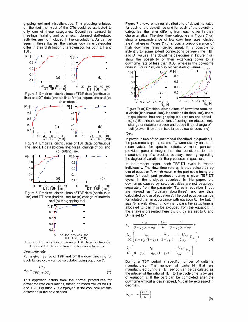
gripping tool and miscellaneous. This grouping is based on the fact that most of the DTs could be attributed to only one of these categories. Downtimes caused by meetings, training and other such planned staff-related activities are not included in the calculations. As can be seen in these figures, the various downtime categories differ in their distribution characteristics for both DT and TBF.

Figure 3: Empirical distributions of TBF data (continuous line) and DT data (broken line) for (a) inspections and (b)

short stops.

Figure 4: Empirical distributions of TBF data (continuous line) and DT data (broken line) for (a) change of coil and

(b) cutting line.

Figure 5: Empirical distributions of TBF data (continuous line) and DT data (broken line) for (a) change of material

and (b) the gripping tool.

Figure 6: Empirical distributions of TBF data (continuous

line) and DT data (broken line) for miscellaneous.

Downtime rate

For a given series of TBF and DT the downtime rate for each failure cycle can be calculated using equation 7.

jj

jS DTTBF

DTq

j

(7)

This approach differs from the normal procedures for downtime rate calculations, based on mean values for DT and TBF. Equation 7 is employed in the cost calculations described in the next section.

Figure 7 shows empirical distributions of downtime rates for each of the downtimes and for each of the downtime categories, the latter differing from each other in their characteristics. The downtime categories in Figure 7 (a) show a preponderance of low downtime rates (circled area), whereas Figure 7 (b) shows a preponderance of high downtime rates (circled area). It is possible to indentify to some extent connections between the TBF and DT values. The downtime categories in Figure 7 (a) show the possibility of their extending down to a downtime rate of less than 0.05, whereas the downtime rates in Figure 7 (b) display higher starting values.

Figure 7: (a) Empirical distributions of downtime rates as a whole (continuous line), inspections (broken line), short stops (dotted line) and gripping tool (broken and dotted

line) (b) Empirical distributions of cutting line (dotted line), change of material (broken and dotted line), change of coil (broken line) and miscellaneous (continuous line).

Costs

In previous use of the cost model described in equation 1, the parameters qQ, qS, qP and Tsu were usually based on mean values for specific periods. A mean part-cost provides general insight into the conditions for the manufacturing of a product, but says nothing regarding the degree of variation in the processes in question.

In the present paper, each TBF-DT cycle is treated individually. The downtime rate qS is thus calculated by use of equation 7, which result in the part costs being the same for each part produced during a given TBF-DT cycle. In the analyses described in this paper, the downtimes caused by setup activities are not described separately from the parameter Tsu as in equation 1, but are viewed as “ordinary downtimes” and are thus calculated by use of equation 7. The cost equation can be formulated then in accordance with equation 8. The batch size N0 is only affecting how many parts the setup time is allocated to, can thus be excluded from the equation. In the analysis presented here qQ, qP, qB are set to 0 and URP is set to 1.

pbRP

RP

PSQ

D

pbRP

RP

S

S

PQ

CS

PQ

CP

BQ

Bj

TU

U

qqq

tk

TU

U

q

q

qq

tk

qq

tk

qq

kk

j

j

j

1

)1)(1)(1(60

1

)1()1)(1(60

)1)(1(60)1)(1(

0

0

00

(8)

During a TBF period a specific number of units is manufactured. The number of parts Nc that are manufactured during a TBF period can be calculated as the integer of the ratio of TBF to the cycle time t0 by use of equation 9. If the part can be completed after the downtime without a loss in speed, Nc can be expressed in decimals.

0t

TBFtruncN

jcj

(9)

0 20 40 60 80

0.2

0.4

0.6

0.8

1P[-]

DT, TBF [min] 0 20 40 60 80 100

0.2

0.4

0.6

0.8

1P[-]

DT, TBF [min]

0 20 40 60 80 100

0.2

0.4

0.6

0.8

1P[-]

DT, TBF [min] 0 10 20 30 40

0.2

0.4

0.6

0.8

1P[-]

DT, TBF [min]

0 10 20 30 40 50

0.2

0.4

0.6

0.8

1P[-]

DT, TBF [min] 0 100 200 300

0.2

0.4

0.6

0.8

1P[-]

DT, TBF [min]

0 100 200 300 400 500

0.2

0.4

0.6

0.8

1P[-]

DT, TBF [min]

0 0.2 0.4 0.6 0.8 10

0.2

0.4

0.6

0.8

1P [-]

qS [-] 0 0.2 0.4 0.6 0.8 1

0

0.2

0.4

0.6

0.8

1P [-]

qS [-]

(b)(a)

(a) (b)

(a) (b)

(b)(a)

The maximum number of parts that can be manufactured during a follow-up period is obtained by the ratio of the sum of all TBFs to the cycle time t0 of the part in question.

Figure 8 shows the number of parts produced during a TBFj at cost kj. Several TBF periods can produce the same amount of parts Nc, but at differing costs kj. In the figure the minimal part costs kmin and the mean part costs kmean are plotted. kmin is the part costs with qS=0 and kmean the part cost with the mean value of qS.

Figure 8: The part costs kj shown as a function of the number of parts manufactured during a TBF period, Nc.

Figure 9 shows the part costs as a function of DT. As it is evident, there is no clear relationship between part costs and the lengths of the downtimes.

Figure 9: The part costs kj as a function of DT.

To increase the performance of a manufacturing system, actions to lower kmean should be carried out. Lowering kmean can be achieved in various ways, depending on the strategy employed. For example, kmean can be lowered by lowering kmin, thus reducing the part costs by considering parameters other than qS. It can also be lowered by lowering the highest kj values. This way of looking at production development can also be illustrated by considering the graph in Figure 10, in which the empirical distribution function for part costs is plotted. kmean can be lowered both by lowering the high part costs shown at the right in the figure or by making changes that affect all the parts, thus pulling kmin, so to speak, to the left. No general advice or conclusions can be formulated, each case needing to be studied in a thorough way individually.

Figure 10: The empirical distribution of all part costs.

Figures 11-14 show the empirical distributions of the part costs related to each of the downtime categories.

Figure 11: The empirical distributions of part costs related

to (a) inspections and (b) short stops.


to (a) change of coil and (b) cutting line.


to (a) change of material and (b) gripping tool.


to the miscellaneous category.

The cost calculations above show how part costs vary as a function of downtimes. In selecting projects aimed at improvement, it is important not only to know how the costs vary but also to know the total cost reduction potential. Figure 15 (a) shows the total downtime costs for every downtime category and Figure 15 (b) shows the downtime costs as a histogram. It can be stated from the figures that the shorter stops are dominating, but they are on the other hand consisting of several different downtime categories. From Figures 11-14 and Figure 15 (a) it is clear that the miscellaneous category from a cost point of view is the largest category. This category constitutes of different kinds of stops that occur relatively seldom, making it presumably more complex and difficult to reduce the costs for this category. The possible measures to take to reduce the costs also must be analyzed together with the expenditures associated with them.

0 50 100 150 200 250 3006

7

8

9

10Part cost[US $/unit]

kmean

kmin

Nc

[units]

0 5 10 15 20 256

7

8

9

10Part cost[US $/unit]

kmean

kmin

DT [min]

6 8 10 12 140

0.2

0.4

0.6

0.8

1P[-] kmean

kmin

Part cost [US $/unit]

0 15 30 45 60

0.2

0.4

0.6

0.8

1P[-]

Part cost [US $/unit]0 5 10 15 20

0.2

0.4

0.6

0.8

1P[-]


0 5 10 15 20 25 300

0.2

0.4

0.6

0.8

1P[-]

Part cost [US $/unit]0 10 20 30 40 50

0.2

0.4

0.6

0.8

1P[-]


0 10 20 30 40 50

0.2

0.4

0.6

0.8

1P[-]

Part cost [US $/unit]0 50 100 150 200

0.2

0.4

0.6

0.8

1P[-]


0 50 100 150 200 250 300

0.2

0.4

0.6

0.8

1P[-]


(a) (b)

(b)(a)

(a) (b)

Figure 15: The total downtime costs for every downtime

category (a) where A is inspections, B short stops, C change of coil, D cutting line, E change of material, F

gripping tool, G miscellaneous and (b) the total downtime costs divided into a histogram.

5 DISCUSSION AND CONCLUSIONS

The authors have endeavored to illustrate here, by use of the concept of dynamic manufacturing how manufacturing costs can be used to describe the variability of a manufacturing process. Translating variability to costs serves to make it particularly evident how important it is to reduce variability.

In this work a TBF period is connected to the successive DT period. The authors are aware of the fact that there not always exist a clear relation between the TBF period and the DT period, a downtime can for example be caused by wear, starting many TBF periods before the downtime occur.

6 FURTHER WORK

Reduction in downtime can be carried out in two ways, either by reducing DT or by increasing TBF. In this paper the TBF is defined as the time between two successive downtimes. Further work will be focused on the time between failures of the same kind and investigate variables affecting this time.

7 ACKNOWLEDGEMENTS

This work has been carried out within the Sustainable Production Initiative.

8 REFERENCES

[1] Ljungberg, Ö., 1998, Measurement of overall equipment effectiveness as a basis for TPM activities, International Journal of Operations & Production Management, 18/5:495-507.

[2] Patty, A.L., Watson, K., 2009, Downtime variability: the impact of duration-frequency on the performance of serial production systems, International Journal of Production Research, 1-11.

[3] Nakajima, S., 1988, Introduction to TPM, Productivity Press, Cambidge, MA.

[4] De Smet, R., Gelders, L., Pintelon, L., 1997, Case studies on disturbance registration for continuous improvement, Journal of Quality in Maintenance Engineering, 3/2, 91-108.

[5] Magnusson, K., Kroslid, D., Bergman, B., 2000, Six Sigma – The Pragmatic Approach, Studentlitteratur, Lund.

[6] Banuelas, R., Tennant, C., Tuersley, I., Tang, S., 2006, Selection of six sigma projects in the UK, The TQM Magazine, 18/5, 514-527.

[7] Vineyard, M., Amoako-Gyampah, K., Meredith, J.K., 1999, Failure rate distributions for flexible manufacturing systems: An empirical study,

European Journal of Operational Research, 116, 139-155.

[8] Yazhou, J., Molin, W., Zhixin, J., 1995, Probability distribution of machine center failures, Reliability Engineering and System Safety, 50, 121-125.

[9] Das, K., 2008, A comparative study of exponential distribution vs Weibull distribution in machine reliability analysis in a CMS design, Computers & Industrial Engineering, 54, 12-33.

[10] Dallery, Y., 1994, On modelling failure and repair times in stochastic models of manufacturing systems using generalized exponential distributions, Queueing Systems, 15, 199-209.

[11] Mohanty, R. P., 1991, Availability Management: Concepts, Evaluation and Strategic Directions, International Journal of Quality & Reliability Management, 8/4, 25-38.

[12] Williams, E.J., 1994, Downtime data – Its collection, analysis, and importance, Proceedings of the 1994 Winter Simulation Conference, 1040-1043.

[13] Skoogh, A., 2009, Methods for Input Data Management – Reducing the Time-Consumption in Discrete Event Simulation, Chalmers Reproservice, Göteborg.

[14] Lamberson, L.R., Wasserman, G.S., 2001, Monitoring manufacturing system availability, International Journal of Production Research, 39/4, 727-736.

[15] Koltai, T., Lozano, S., Guerrero, S., Onieva, L., 2000, A flexible system for flexible manufacturing systems using activity based costing, International Journal of Production Research, 38/7, 1615-1630.

[16] Ioannou, G., Sullivan, W.G., 1999, Use of activity-based costing and economic value analysis for the justification of capital investments in automated material handling systems, International Journal of Production Research, 37/9, 2109-2134.

[17] Özbayrak, M., Akgϋn, M., Tϋrker, A.K., 2004, Activity-based cost estimation in a push/pull advanced manufacturing system, International Journal of Production Economics, 87, 49-65.

[18] Murty, A.S.R., Naikan, V.N.A., 1995, Availability and maintenance cost optimization of a production plant, International Journal of Quality & Reliability, 12/2, 28-35.

[19] Calabria, R., Pulcini, G., Rapone, M., 1995, Optimal reliability and maintainability allocation in manufacturing systems, Quality & Reliability Engineering International, 11, 183-188.

[20] Jones, B., Jenkinson, I., Wang, J., 2009, Methodology of using delay-time analysis for a manufacturing industry, Reliability Engineering and System Safety, 94, 111-124.

[21] Sherif, Y.S., Kolarik, W.J., 1981, Life Cycle Costing: Concept and Practice, OMEGA The International Journal of Management Science, 9/3, 287-296.

[22] Jönsson, M., Andersson, C., Ståhl, J.-E., 2008, A general economic model for manufacturing cost simulation, Proceedings of the 41st CIRP Conference on Manufacturing Systems.

F E

C D

G

B

A

[US $]

0 100 200 3000

5000

10000

15000

[US $]

[minutes]

Implementation of an Economic Model to Simulate Manufacturing Costs


Division of Production and Materials Engineering, Lund University, Sweden

Abstract An economic model describing manufacturing costs is implemented within the frame of a case study. The implemented economic model is developed to enable analyses of the cost items and parameters influencing the cost of a part or a batch and also to make simulations for the purpose of investigating the economic outcome of future development activities. The aim of the case study was to identify activities in a production unit that could lead lower manufacturing costs by using the method described in this paper. Keywords: Manufacturing Economy; Cost Model; Economic Simulation

1 INTRODUCTION The globalisation has influenced the manufacturing sector considerably; it has become more important than ever to constantly increase the productivity in the manufacturing plants to be able to meet the increasing competition, especially from companies in low-wage countries. Many companies deal with these circumstances by offshoring or by offshore outsourcing. These types of relocations are solely based on cost reductions, in contrast to relocations based on market aspects for the purposes of getting closer to a certain market for competitive reasons. But to relocate the manufacturing plants to low-wage countries doesn’t have to be the only way out to maintain a high competitiveness for companies in countries with high wages. Focusing on the optimal production development regarding organizational issues and production technology can in many cases compensate the higher level of wage costs. In order to make the right decisions concerning the offshoring based on cost reductions, it is necessary to be able to make correct analyses of the performance in the manufacturing plant from an economic point of view. One approach is to analyse the manufacturing costs of the products produced in the plant. Common methods to calculate the manufacturing costs are the traditional full costing methods and Activity-Based Costing (ABC). Traditional full costing is mostly used for cost-price calculations and is not an equally suitable method to use when seeking detailed and accurate information solely about the manufacturing costs, essentially because of the methods volume based approach. One of the main purposes behind the development of ABC was to in a more accurate way than traditional full costing allocate the overhead costs [1]. A lot of research has been done over the years since ABC was first introduced with the intention of implementing and analyzing the method, for example Thyssen, et al. [2].

The model presented in this paper is developed with the purpose of calculating and analysing the part cost associated with the manufacturing. The model has some similarities to ABC, for example when it comes to recognising the cost of unused capacity and the different types of parts individual consumption of the manufacturing resources. The main differences are that the model presented here only describes costs related to manufacturing. The focus of this model is to describe the relations between economy and manufacturing performance. Another difference is that this model allocates batch level activities to the unit level and also allocates cost of unused capacity to products. Models describing the manufacturing cost can roughly be divided into a micro- and macroeconomic approach according to Tipnis, et al. [3]. The macroeconomic models are essentially based on aggregated information while the microeconomic models include process data like cut rate, gas flow, current intensity etc. For example Colding [4], [5], Alberti, et al. [6] and Knight and Poli [7] have all described microeconomic models while Groover [8] has described a macroeconomic model. The model applied below can be described as a macroeconomic model. The applied model differs from the models presented in the previous section by the inclusion of all the production loss parameters; scrap rate, down time rate and production rate. 2 PURPOSE The performance of a defined production unit that manufactures gearwheels will be analysed, using a manufacturing economic model described in section 6. The purpose was to identify activities in the production unit that can lead to lower manufacturing costs by using the method described in this paper.

The 41st CIRP Conference on Manufacturing Systems, 2008

39


3 METHOD To be able to test the model in real a context a case study at a company was considered as the most appropriate choice of method. The case study was chosen to be limited to one section at the factory in order to make the data collection manageable from a practical perspective and it was also considered sufficient in order to to comply with the purpose of the study. The case study began with a careful study of the chosen production unit to get an understanding about its characteristics regarding the process and function. The accuracy of the economic data obtained by the cost model is dependent on the accuracy of the collected data. Therefore a systematic data collection was made regarding the scrapped parts, down time, production rate and the set up time. 4 SYSTEMATIC PRODUCTION ANALYSIS The systematic data collection mentioned in section 3 was performed by implementing a method called Systematic Production Analysis (SPA) [9]. The method has been developed to determine the existing production condition. In this method the result parameters downtime rate, scrap rate and production rate are measured for each processing unit involved in the manufacturing of a specific product. The possible downtime, scrapped parts and loss in production rate are related to a factor found in one of the following factor groups: A Tool and tooling system; B Work piece material; C Manufacturing process and process data; D Personnel, organization and outer logistics; E Maintenance and wear tied to A, C, D and G; F Special process behavior/factors; G Surrounding equipment and inner logistics; H Unknown or unspecified factors Table 1 shows a method of presenting a SPA. Q1 to Qn describe different quality deviations leading to scraped parts, where every Q has a separate column. Analogous to the quality parameters, S1 to Sn describe different types of down time losses and P1 to Pn describe different production rate deviations. The factor groups describe causes leading to the different result parameters. Every factor group contain individual factors, for example factors A1 to An, where every individual factor has a separate row. After an implantation of this method, where every disturbance has been registered in the right place in the table, you can sum up the result for every row and column and then find critical result parameters and factors for the specific processing unit. This method makes it possible to directly get an indication towards which of the result parameters and which of the individual factors that causes losses in the production efficiency. Coupling this to economic parameters it is possible to determine the part cost under the influence of the result parameters. In section 6 it will be shown how these result parameters together with time and batch size parameters and also economic data build up the part cost in a specific processing step.

Table 1: Systematic production analysis.

Result parameters

Factor groups

Q1,..,Qn (unit)

S1,...,Sn (min)

P1,...,Pn (min)

�

A1,...,An

B1,...,Bn

C1,...,Cn

D1,...,Dn

E1,...,En

F1,...,Fn

G1,...,Gn

H

�

5 LIST OF SYMBOLS

Table 2: List of symbols used in this paper. The economic parameters is described in the Swedish currency krona (kr).

Parameter Description Unit t0 Nominal cycle time per part min

tm Machine time min

th Handling time min

tvb Tool switch time min

NQ Amount of scrap parts in a batch of N parts

unit

N Total batch size, including scrap parts

unit

N0 Amount of correct produced parts in a batch

unit

qQ Scrap rate -

tp Production time per part min

tS Average down time per part min

qS Down time rate -

qP Production rate -

t0v Cycle time including production rate losses

min

Tsu0 Nominal set up time min

Tsu Set up time including deviations from nominal set up time

min

qSsu Ratio between the nominal set up time Tsu0 and the real set up time Tsu

-

k Part cost kr/unit

kA Tool cost kr/unit

kB Material cost kr/unit

kCP Equipment cost during production kr/h

kCS Equipment cost during downtime and set up

kr/h

kD Wage cost kr/h

xp Process development factor for the cycle time

-

40


xsu Process development factor for set up time

-

�c Equipment cost development factor

-

�z Change in an arbitrary variable z -

kVA Value added part of the part cost kr

kNVA Cost of non value added activities kr

kTsu Costs related to set up kr

kQ Costs connected to the scrap rate kr

kS Costs related to the down time rate kr

kP Costs connected to the production rate

kr

6 ECONOMIC MODEL The economic model is priviously described in [9]. In this section a summerized description is presented. The nominal cycle time t0 in a machine or a line is defined in equation 1, tm is the machine time, th handling time and tvb tool change time.

vbhm tttt ��0 (1)

The scrap rate qQ is defined in equation 2, where NQ is the number of scrap parts, N is the batch size and N0 the number of correct, non scrapped parts of the batch.

NNN

NN

q QQ

0�� (2)

The down time rate qS is defined in equation 3, where ts is the down time per cycle and tp the actual cycle time.

p

p

p

ss t

ttttq 0�

�� (3)

The production rate qP describes the ratio between the nominal cycle time t0 and the real cycle time tv and is defined in equation 4.

vP t

tq0

01�� (4)

The downtime rate during set up qSsu describes the ratio between the nominal set up time Tsu0 and the real set up time Tsu, see equation 5.

su

suSsu T

Tq 01�� (5)

The production time for a batch including the setup time can then be defined as in equation 6:

)1)(1()1(00

PSSsu

supb qq

tNq

TT��

��

�� (6)

Reduced occupation in a manufacturing system leads to consequences for all manufactured parts. This situation can be considered in different ways, hence the free production resource can be considered both as an economic asset and a disadvantage depending on the situation. In a long term view the manufactured parts must carry the costs for the over capacity. The over capacity time can be distributed over all the batches in relation to their production time Tpb by introducing a degree of occupation URP, calculated as the

quotient between real production time Tprod and planned production time Tplan according to according to equation 7 and 8. Tfree is the time for the free, non occupied production time.

freeprodplan TTT �� (7)

plan

prodRP T

TU � (8)

The extra free capacity Tfree,b to be added to a specific batch is calculated according to equation 9. The free time can be considered as a setup time at the same time as the equipment is available for manufacturing:

pbRP

RPbfree T

UUT �

�1

, (9)

With these parameters together with economic data, the cost of production per part can be calculated. The economic parameters included in the model is the following : �� Tool cost kA �� Material cost kB �� Equipment cost during production kCP �� Equipment cost during down time and set up kCS �� Wage cost kD The cost of production per par can then be calculated using equation 10.

��

��

��

��

��

��

��

��

��

��

��

��

��

��

��

��

��

��

��

��

pbRP

RP

Ssu

su

Q

D

PSQ

D

pbRP

RP

Ssu

su

Q

CS

S

S

PQ

CS

PQ

CP

Q

B

PQ

A

TU

Uq

TqN

k

qqNt

qNk

TU

Uq

TqN

k

qq

qNt

qNk

qqNNtk

qNNk

qqNNkk

1)1()1(60

)1()1()1(60

1)1()1(60

)1()1()1(60

)1()1(60

)1()1()1(

0

0

0

0

0

(10)

To be able to simulate the effect of an improvement of the production process, a number of factors are introduced. The development factors are xp, xsu and the cost factor �c, where xp describe the improvement in cycle time that is achieved due to the development of the process. Likewise, xsu describes the improvement in set up time. �c is used to model changes in costs in primarily existing equipment, and can be used to determine the limit of investment justified to for example a decrease of the downtime rate to a certain value. The manufacturing economic model including development and cost factors is described in equation 11.

41


��

��

��

��

��

��

��

��

��

��

��

��

��

��

��

��

��

��

��

��

��

��

pbRP

RP

Ssu

susu

Q

D

PS

P

Q

D

pbRP

RP

Ssu

susu

Q

CSC

S

S

P

P

Q

CSC

PQ

PCPC

Q

B

PQ

A

TU

UqTx

qNk

qqNtx

qNk

TU

UqTx

qNk

qq

qNtx

qNk

qqNNtxk

qNNk

qqNNkk

1)1()1(60

)1()1()1(60

1)1()1(60

)1()1()1(60

)1()1(60

)1()1()1(

0

0

0

0

0

�

�

�

(11)

Changes in part cost caused by a limited change in an arbitrary variable z, is calculated by partial derivative, and is described in linear form in equation 12.

zz

kk ni ��

��

�� (12)

Cost neutral changes in each variable can be studied by putting the change in part costs �ki = 0. Equation 12 is written in a cost neutral form in equation 13, describing the size of the reduction in downtime share required to compensate for a change in wage costs.

Si

i

Di

i

DiSi

qk

kk

kq

��

�� (13)

7 THE CASE STUDY The implementation of the method SPA resulted in data connected to a number of products produced at the factory at the choosen manufacturing unit. This paper will present an analysis of one of these products, called product x. Besides as an analysis of this product, this case study presentation also can be viewed as an example of how you can apply the cost model described in equation 11, when an SPA has been made and other necessary production data is available. From the data collection phase of the case study, including a systematic registration of scrap, down time and production rate according to the method described in section 4, the values of the parameters in equation 10 was obtained and is presented in Table 3. In this case study the cost of reduced occupation has not been considered and there is no data for the deviation from the nominal set up time for this product. Inserting the values of the parameters in Table 3 into equation 10, the cost of production per part k equals 386,8 kr, which implies that this processing step adds 144,27 kr to the cost of the product.

Table 3 : Calculated values of the parameters in the economic model

qQ qS qP qSsu Tsu0 t0

0.0230 0.4273 0 0 120 7.2

N0 kA kB kCP kCS kD

1000 13.7 242.53 420 420 150

During the analysis of the collected data, new ways to present the costs was developed. This was done by starting out from equation 10 and then divide the cost k into the different parts that add costs in the chosen processing step. The chart in Figure 1 below shows the part cost k together with kB and these new cost items; kVA, kNVA kTsu, kQ, kS, and kP, where k equals the sum of kB, kVA, kNVA and kTsu, see equation 14.

TsuNVAVAB kkkkk �� (14)

Figure 1: The part cost k and different parts of k. kVA is the value added part of the cost and is defined in equation 15. kVA describes the cost added in this processing step, without considering qQ, qS, qP and Tsu.

� � 0tkkkk DCPAVA �� (15)

kNVA is the cost of non value added activities and constitutes of all costs related to the loss parameters qQ, qS and qP, and is defined in equation 16.

PSQNVA kkkk �� (16)

kTsu constitutes of the costs related to set up and is defined in equation 17.

)1()1(600

Ssu

su

Q

DCSTsu q

TqN

kkk�

��

�� (17)

By dividing the part cost k into kB, kVA, kNVA and kTsu you get a quick overview of the cost condition of the product. The size of kNVA indicates the potential cost reduction by decreasing the disturbances in the production. kNVA make up 42.3 % of the total cost added in this processing step, or 61.0 kr per part. Correspondingly, kVA make up 56.9 % of the total cost added, or 82.1 kr expressed in cost per part. kTsu is calculated to 1.2 kr per part. The combination of a large batch size and a long cycle time makes kTsu relatively insignificant regarding the part cost of product x at this chosen processing step. A division of kNVA can be made into kQ, kS and kP, with the purpose to find out the specific costs contributed by each

k kB kVA kNVA kTsu kQ kS kP

200

300

100

0

kr

42


result parameter qQ, qS, qP. kQ describes the costs connected to the scrap rate qQ and is defined in equation 18.

�

��

��

��

��

6060)1(00 tktkkk

qNqN

k DCPBA

Q

QQ (18)

The largest part of kNVA consists in this case of costs related to the down time rate qS. This cost is named kS and is defined in equation 19. kS was calculated to 52.7 kr per part and constitutes 86.3 % of kNVA.

)1()1()1(60

)1()1()1(60

0

0

PSQ

SD

PSQ

SCSS

qqqNqNtk

qqqNqNtkk

��

��

��

(19)

kP describes the costs caused by qP and is defined in equation 20 and was calculated to 0.7 kr per part.

)1()1(60

)1()1(60)1()1(

0

0

PQ

PD

PQ

PCP

PQ

PAP

qqNqNtk

qqNqNtk

qqNqNkk

��

��

��

��

�

(20)

The size of kNVA for this product at this production unit implies that there is a substantial amount of money to be saved if kNVA can be reduced, if the total annual volume of the product is considered. The annual volume of product x is estimated to 9300 units by the company. If assuming that the value of kNVA is intact over a year, the theoretical cost reduction becomes roughly: 5673009300619300 ��NVAk kr.

To reduce kNVA you have to know the result parameters and the factors connected to these parameters that together constituting the value of kNVA. When combining the result from the SPA and the parameters calculated from this data, it will be possible to obtain the influence on the manufacturing cost of every result parameter and factor registered in the SPA. In Figure 2 the factors having the largest effect on the part cost of product x as a result of the performed SPA are shown as their cost per part. The figure illustrates that apart from the tool factor A2, the major factors behind the size of kNVA are related to the process C and organizational issues D.

Figure 2: The factors having the largest effect on the part cost

of product x

After quantifying the cost of the production disturbances and the factors in the different units or cells of the manufacturing plant, it will be possible to compare different disturbances influence of the manufacturing cost and thereby for example

be able to make priorities between different development projects concerning the manufacturing process.

At this stage, when the critical parameters and factors connected these losses are obtained and economically quantified, then cost derivatives can be used to analyse different development scenarios. Figure 3 illustrate the cost neutral relationship between a change in the development factor ��C and a change in downtime rate �qS for product x. The figure shows for example that if the down time rate can decrease by 0.15, you get ��C to 0.35. This means that the equipment costs, kCS and kCP, can be increased by up to 35 % without increasing the part cost if the decrease in qS can be accomplished.

0.250.20.150.10.05

Figure 3: Cost neutral change between an increase in equipment cost factor ��C and reduction of down time rate

�qS. As Figure 2 illustrates, the largest cost factor for product x is A2, which is a factor connected to the tools in the machine. Figure 4 shows the cost neutral relationship for product x between an increase of the tool cost �kA and a decrease of the process development factor �xP. This relationship illustrates the maximum cost increase of improved tooling capable of reducing the cycle time to a certain level. The dotted graph shows the relationship when new but more expensive tools enables a decrease in xP, but at the same time causes an estimated increase in the scrap rate qQ by 0.01. The continuous graph shows the relationship without any increase in qQ.

0.140.120.10.080.060.040.020

0

Figure 4: Cost neutral changes between an increase in tool cost �kA and reduction of the development factor �xP (continuous graph) and an increase in �kA plus a 0.01 increase of qQ and a reduction of �xP (dotted graph).

This analysis is made for a single product in a processing step where several other products is produced. These other products and the costs connected to them must of course be

-0.05 -0.1 -0.15 -0.2 -0.25

��C

0.8

0.6

0

0.2

0.4

�qS

0 -0.04 -0.08 -0.12 0

8

6

4

2

�xP

�kA

E18 A2 D5 C17 C22 C8 D8 C5

10

8

6

4

2

0

kr

0

43


taken into consideration to get a general picture of the costs in this processing step. 8 DISCUSSION AND CONCLUSIONS To sum up the analysis described in the previous section, the high value of qS is making a significant impact on the manufacturing cost of this product at this processing step. This case study shows that there is a potential in analysing the manufacturing performance of today and alternative simulated scenarios with the method described in this paper. An important prerequisite for these analyses to be reliable is the accuracy of the input data and how detailed this data is. If the model is implemented at every unit or cell at a factory it will then be possible to obtain which cost items that builds up the total manufacturing cost of a part or a group of parts and size of these items. Figure 5 shows the division of the part cost k made in section 7. This division makes it easy to get a clear view of the costs added in a processing step. Having this detailed information accessible for products in all processing steps would enabeling a greater insight and understanding about where in the manufacturing process there is the highest potential to lower the costs and thereby function as a basis for prioritys concerning production development activities.

k

kB kVA kNVA kTsu

kQ kS kP

SPA kS1,…,kSn kA1,…,kH

Figure 5: The division of k made in the presented case study

analysis.

By combining production data and economic data into this economic model it is also possible to establish manufacturing economic development goals. A development goal could for example be to reduce the cost of manufacturing per part with 10 % for a product or a group of products. By the implementation of this model a plan to reach that goal could be established. 9 REFERENCES [1] Cooper, R., Kaplan, R.S., 1992, Activity-Based

Systems: Measuring the Costs of Resource Usage, Accounting Horizons, 6/3:1-13.

[2] Thyssen, J.T., Israelsen, P., Jorgensen B., 2006, Activity-based costing as a method for assessing the economics of modularization – A case study and beyond, International journal of production economics, 113:252-270.

[3] Tipnis, V.A., Mantel, S.J., Ravignani, G.J., 1981, Sensitivity Analysis for Macroeconomic and Microeconomic Models of New Manufacturing Processes, Annals of the CIRP, 30:401-404.

[4] Colding, B., 1978, Relative Effects of Shop Variables on Manufacturing Cost and Performance, Annals of the CIRP, 27:453-458.

[5] Colding, B., 2003, Tids- och kostnadsanalys vid skärande bearbetning – Optimering för synkront detaljflöde, Colding International Corporation, Stockholm.

[6] Alberti, N., Noto La Diega, S., Passannanti, A., 1985, Interdependence between Tool Fracture and Wear, Annals of the CIRP, 34:61-63.

[7] Knight, W.A., Poli, C.R., 1982, Design for Economical Use of Forging: Indication of General Relative Forging Costs, Annals of the CIRP, 31:159-163.

[8] Groover, M.P., 1987, Automation, Production Systems, and Computer Integrated Manufacturing, Prentice-Hall Inc, Englewood Cliffs, NJ.

[9] Ståhl, J.-E., 2007, Industriella Tillverkningssystem, Division of Production and Materials Engineering, Lund University, Lund.

44

Conditions for and development of an IT-support tool for manufacturing costs calculations and analyses


Division of Production and Materials Engineering, Lund University, Lund, Sweden

Abstract

Collecting data on manufacturing performance and making the results known to

those involved could support efforts to improve manufacturing processes. This

paper describes the conditions for and development of manufacturing cost

software developed for analyzing connections between manufacturing

performance parameters and economic parameters. The conditions for the

software were investigated in two pre-studies. The first found that there are

commercial software products for manufacturing data collection that support the

collection of the data needed for the applied model. The second study

demonstrated that the manufacturing companies participating in the second study

were largely able to collect the needed data. The developed software,

preliminary in character and needing further development, provides information

on how the manufacturing performance of a company affects its manufacturing

costs. It takes account of six categories of manufacturing cost. A what-if section

is included, making it possible to alter the values of various parameters that

affect costs in order to analyze how the part cost of a certain component changes

with the use of new parameter values compared with historic values.

Keywords: cost analysis, cost improvement, performance measures, manufacturing

management

1. Introduction

Staying competitive in a global market is a necessity for any manufacturing company today.

Success in doing so is strongly dependent on the ability to develop innovative products and to

design flexible and optimally performing manufacturing systems. A manufacturing system

represents a highly complex system consisting of a variety of components, such as machines,

tools, material-handling equipment, control systems, and operators. The management and

improvement of such complexity requires true and relevant data on the performance and

outcome of the system and its individual components. A widely used performance measure in

the manufacturing industry is overall equipment effectiveness (OEE), originally introduced by

Nakajima (1988). The monitoring of OEE often involves the use of data collection software of

some sort for collecting data and calculating performance in terms of, for example, quality

rate, equipment availability, and equipment utilization.

The challenges of global competition for manufacturing companies require that they

increase their cost awareness. Differences in wage levels between various parts of the world

have led many companies in the western world to turn to offshore production or to outsource

their production to countries with lower wage levels. Such relocation is inevitable in the case

of, for example, non-complex products with low value added or when striving for new market

shares. However, outsourcing might not have been done to the extent it was in the early 00s if

a complete set of factors (not only wage costs) influencing the total manufacturing cost had

been considered. In fact, factories paying fairly high wages can be competitive, through using

appropriate manufacturing strategy and by excelling in productivity and performance.

Production development with high cost awareness can provide opportunities to set appropriate

priorities regarding the development activities having the largest impact on cost efficiency.

This requires correct information about all the parameters that drive costs in the production

system.

There is a lack of adequate cost models describing the links between performance

parameters and the manufacturing costs involved. Most cost models presented in the literature

contain too little detail regarding the parameters that affect various manufacturing costs. There

are however exceptions, for example the models by Son (1991), Chiadamrong (2003), and

Yamashina and Kubo (2002) are quite comprehensive, but they lack a clear link to

performance parameters. Also the practical aspects of these models are not considered, i.e. the

conditions for industrial implementation of the models and how the models should be used by

the practitioner in the industry.

The authors of this paper have developed a cost model (2008a,b) that links production

performance parameters with economic parameters, enabling detailed analysis of the

manufacturing costs of specific parts or products. The model is intended for use by plant

management as a tool for strategic decisions regarding priorities for manufacturing

development action, production sourcing and to generally increase the cost awareness in the

manufacturing department of a company.

2. Research questions and method design

As stated above there are detailed cost models in the literature, but practical aspects regarding

usability are often treaded rather briefly. A cost model indented to be used in the industry is of

limited value if it is not practicably usable. It was therefore considered necessary to take

account of these aspects, i.e. to investigate the conditions for implementing the cost model

(2008a,b) in an industrial environment.

Implementation encompasses two important aspects: availability of input data for the

cost model and how the model should be implemented. This paper addresses both issues by

investigating whether the needed input data can be collected from existing company

databases. Using a detailed manufacturing cost model to analyze manufacturing costs makes

considerable demands of the data collection systems in place and of company data collection

routines, in order to provide the analysis with correct information about the manufacturing

process being analyzed.

The paper also addresses the design of the manufacturing cost software to meet

requirements for usability, result visualization, and simulation capability. The aim of this

research can be formulated in two research questions:

RQ1: What are the conditions for a successful industrial implementation of the cost

model in terms of the functionality of data collection systems available on the market,

and to what extent do companies already collect the needed data?

RQ2: What are the specific requirements for user-friendliness for an industrial

implementation of the cost model, what analysis and simulation capabilities should be

provided for the user, and how should the results be presented and visualized?

To answer the first question, we reviewed various commercial data collection systems

concerning their support for collecting the required data. A case study involving five

companies was also performed to consider the extent to which these data were collected at the

studied companies. These pre-studies were conducted by means of interviews and by

examining the systems in place.

To answer the second question, we performed a case study to develop a manufacturing

cost software application together with one of the manufacturing companies participating in

the pre-study. According to Yin (2006) case studies enable phenomena to be studied in their

real-world contexts, and it was precisely the real-world context we wanted to consider by the

above stated research questions. It was therefore decided that the best way to find out how

such a software application should be designed was to develop one, and to do so in

collaboration with a company that was an intended user of the software. The advantages with

incorporating prototype development in the research process is for example discussed by

Nunamaker et al. (1991), which argue that a prototype can both constitute a proof of a concept

and also form a base for continued research.

3. Frame of reference

A performance measurement system (PMS) is defined by Neely et al. (1995) as a ‘set of

metrics used to quantify both the efficiency and effectiveness of actions’. Despite an extensive

PMS literature related to manufacturing extending many decades back, there has been a

marked increase in publications in this field over the last 20 years (Neely 2005). According to

Ghalayini and Noble (1996), the PMS literature can be divided into two main phases, the first

extending from the 1880s to the early 1990s and the second, or current phase, covering the

period since then. In the first phase, financial measures were emphasized. In the current phase,

considerable emphasis is placed on the shortcomings of traditional financial measures; the use

of non-financial measures is advocated, although there is no clear consensus among authors as

to which non-financial measures companies should select.

Neely et al. (1995), in reviewing the PMS literature, distinguish four dimensions of

performance measures, those of quality, time, flexibility, and cost. These four dimensions

describe what these authors found that the literature regarded as the most important

dimensions in defining manufacturing performance. White (1996), in his survey of

performance measures, proposes a similar division, but his also includes, along with the four

dimensions just referred to, delivery reliability as a major dimension. White classifies these

five dimensions as competitive capability, and adds four additional dimensions that describe

various aspects of the measures, such as data source and type, as shown in Table 1.

Table 1. White’s (1996) five dimensions of a PMS.

Competitive capability Data type

Cost Subjective

Quality Objective

Flexibility Reference

Delivery reliability Benchmark

Speed Self-referenced

Data source Orientation

Internal Process input

External Process outcome

White concludes that most measures used by companies are internal, objective, and

self-referenced, and have a process–outcome orientation. At the same time, he argues for the

importance of companies’ also obtaining externally based, subjective, benchmark, and process

input-oriented measures and of not simply focusing on cost capabilities, as many companies

have traditionally done.

Arguing as White does for multidimensional measures is common in the second phase

of PMS research. Gomes et al. (2004), in their review of the PMS literature, have constructed

a five-phase framework for the evolution of PMS. The framework they advocate suggests that

development is headed towards multidimensional, balanced, and integrated measures, as well

as towards acceptance of the importance of non-financial measures and of the connection

between these measures and company strategy.

One measure that manufacturing companies commonly employ is OEE. Nevertheless,

the PMS literature seldom treats this measure, possibly because of the previously described

emphasis on multidimensional measures in the PMS literature. OEE focuses on what

Nakajima (1988) calls the ‘six big losses’ due to equipment failure, required setup time, idling

and minor stops, reduced speed, quality defects, and reduced yield. As can be seen, OEE

measures the performance of equipment on the shop floor. OEE is calculated by multiplying

the availability rate, A, by performance efficiency, P, and quality rate, Q. These rates are

defined in equations (1) to (4) below.

amount processed

amountdefect amount processed Q

(1)

timeloading

timeoperatingA

(2)

downtime unplanned timeloading timeoperating (3)

Loading time is the total production time minus planned downtimes, such as planned

maintenance and morning meetings. Unplanned downtimes involve downtimes resulting, for

example, from failures, setup times, and time for die exchange.

timeoperating

timecycle idealamount processed P

(4)

Using White’s categorization as shown in Table 1, OEE then measures various aspects

of quality, flexibility, and speed. OEE is also internal, objective, and self-referenced and

measures process outcome. It fails, however, to use all the proposed dimensions of a

measurement system and needs to be complemented with additional measures, as has also

been noted by Jonsson and Lesshammar (1999). Another shortcoming of OEE is that it

measures only the performance of individual pieces of equipment as such, failing to take

account of the linkages between various machines and the flow of materials within the

manufacturing system. This shortcoming of OEE has been identified by Jonsson and

Lesshammar (1999), Muchiri and Pintelon (2008), and Muthia and Huang (2007). Muthia and

Huang (2007) propose a solution to the insufficiency of measuring pieces of equipment

individually, introducing the term overall throughput effectiveness (OTE). OTE is based on

OEE and can be described as a factory-level version of OEE that takes the dependability of

equipment into account. OTE is expressed in four ways, depending on the characteristics of

the machine layout, such as whether they function in series or parallel.

In their review of the OEE literature, Muchiri and Pintelon (2008) consider various

suggested modifications of OEE, all of which attempt to overcome its various insufficiencies.

The modified measures include production equipment effectiveness (PEE), overall asset

effectiveness (OAE), overall plant effectiveness (OPE), and OTE. Muchiri and Pintelon

(2008) believe that the absence of a cost dimension is a serious shortcoming of OEE and that

future research should explore the translation of equipment effectiveness into costs. They also

believe that future research should investigate the benefits of investing in automated data

collection systems to gather the data needed for OEE calculations.

As stated in the introduction chapter there is a lack of manufacturing cost models

which link performance parameters with costs. Some of the cost models found in the literature

are based on activity based costing (ABC), for example the models by Özbayrak (2004) and

Koltai et al. (2002). ABC models have a tendency on focusing on correct ways to handle

overhead costs and not on how the performance of the manufacturing system affects the cost.

There are also manufacturing cost models not based on ABC, for example the models by

Dhavale (1990), Cauchick-Miguel and Coppini (1996), Branker et al. (2011). The first two

focus on the same aspects as ABC models commonly do, i.e. allocation of overhead costs. The

model by Branker has a clear focus on environmental costs. The three models mentioned in

the introduction chapter, i.e. the models by Son (1991), Chiadamrong (2003), and Yamashina

and Kubo (2002) include costs related to performance, but not as integrated as the model by

Jönsson et al. (2008a,b) in which the performance losses are formulated as rates. Additionally,

these three models describe the cost only as a period cost, not how the cost of the various

products are built up in the processing steps they undergoes.

4. Cost model and data collection method

The cost model to be considered represents the further development of a method for

production data collection and analysis described in detail by Ståhl (2010) and depicted in

Figure 1. The aim of this data collection method is to enable the connections between a

specific production performance parameter (scrap rate, downtime rate, or production-rate loss)

and the factors affecting it to be studied. The factor groups A to H in the figure represent the

causes of the disturbances involved, the Q parameters various quality deviations, the S

parameters downtimes of various types, and the P parameters speed losses of various types.

Converting the Q parameters to loss of time allows sums to be obtained both for separate rows

and columns and for the rows and columns taken together. Collecting the manufacturing input

data for the cost analysis software in accordance with this enables the various considered

parameters and factors to be compared in terms of their impact on manufacturing cost per part

produced. This makes it possible to assign appropriate priorities, based on their effects on

cost, to the various improvement measures that can be undertaken.

Result parameters

Factor

groups

Description Q1 ... Qn

(units)

S1 ... Sn

(min)

P1 ... Pn

(min)

∑

A1 ... An Tool-related

failures

B1 ... Bn Material-related

failures

C1 ... Cn Machine-related

failures

D1 ... Dn Failures-related

to personnel and

organization

E1 ... En Maintenance-

related factors

F1 ... Fn Specific

process-related

factors

G1 ... Gn Factors related

to peripherals

such as material

handling

equipment

H Unknown factors

∑

Figure 1. An overview of the factor- and result-based principles involved in the data collection procedures.

4.1. Cost model

The developed cost model (Jönsson 2008a,b) takes account both of production performance

parameters corresponding to those included in OEE and of cost-related parameters such as

material, equipment, and wage costs. The results of the calculations are expressed in

USD/part. Equation 5 is the version of the model used in the developed software. Because of

the specific configurations of individual manufacturing systems, it is impossible to develop a

completely general model, so the model presented in equation 5 could need modification from

case to case. Compared with the versions included in Jönsson et al. (2008a,b), equation 5

illustrates how the model is to be used in cases involving more than one processing step.

Index i describes the various processing steps; if i = 1, then ki–1 =kB. kB being the material cost

(USD /unit).

)1()1()1()1(60

)1(

1

)1(60

)1()1()1(60

)11(60)1(

1

0

11

0

01

1

i

i

iii

ii

i

i

i

i

i

ii

i

i

ii

ii

ii

ii

i

i

Qi

su

PSQ

D

Qi

pb

RP

RP

Qi

suCS

S

S

PQ

CS

PQ

CP

Q

Qi

ii

qN

T

qqq

tk

qN

T

U

U

qN

Tk

q

q

qq

tk

q()q

tk

q

qkkk

(5)

The parameters in equation 5 are described in Table 2.

Table 2. Description of the parameters in equation 5.

Parameter Description Parameter Description

k (USD /unit) Cost per part Tpb (min) Production time for a batch

kCP (USD /h) Hourly machine cost during

production

Tsu (min) Setup time

kCS (USD /h) Machine cost during

downtimes, setup times, and

idle times

qQ (-) Quality losses due to scrapped

parts

kD (USD /h) Wage cost qS (-) Downtime losses

N (units) Batch size qP (-) Production-rate losses

t0 (min) Nominal cycle time

Costs kCP, kCS, and kD are expressed in cost per hour and t0, Tsu, and Tpb are expressed

in minutes, hence the division by 60 in equation 5 and in some of the equations described

below.

Equation 6 concerns the expression for the scrap rate, qQ where NQ is the number of

scrapped parts in processing step i and Ni is the batch size for processing step i excluding

scrapped parts, i.e. the number of correctly manufactured units in step i.

1

1

1

i

ii

i

Q

QN

NN

N

Nq i

i (6)

The downtime rate in processing step i, qS, is represented in equation 7, where ts is the

downtime per part and tp is the total cycle time, including downtime, i.e. t0 plus ts.

i

ii

i

i

i

p

p

p

s

St

tt

t

tq

0 (7)

Production-rate loss, qP, denotes speed losses due to such factors as machine

instabilities. Equation 8 represents qP where t0v is the nominal cycle time in processing step i

plus any extra time caused by speed losses.

i

ii

i

v

v

Pt

ttq

0

00 (8)

Machine utilization, URP, can be dealt with in various ways, although the authors

maintain that long-term free capacity should be considered a cost. Equation 9 represents the

expression for URP where Tplan is the planned production time in step i and Tprod is the actual

production time in step i.

i

i

i

plan

prod

RPT

TU

(9)

In the part cost equation, the cost of free capacity is distributed over the parts produced

in relation to the production time for the batch, Tpb. Tpb is described in equation 10.

)1()1(

01

ii

i

ii

PS

i

supbqq

tNTT

(10)

The value-added cost per part is represented in equation 11. The value-added cost of a

part is its ideal cost, i.e. the cost of doing things right without any non-value-added costs such

as downtimes or scrapped parts.

i

ii

it

kkk

DCP

VA 060

(11)

The scrap cost per part is defined in equation 12.

)1(6060

00

1

i

iiiii

i

Q

QDCP

iQq

qtktkkk

(12)

The downtime cost per part is defined in equation 13.

)1()1()1(6060

0

iii

iiii

i

PSQ

SDCS

Sqqq

qtkkk

(13)

Equation 14 describes the production-rate loss cost per part.

)1()1(6060

0

ii

iiii

i

PQ

PDCP

Pqq

qtkkk

(14)

Equation 15 describes the setup cost per part.

)1(6060 1 i

iii

i

Qi

suDCS

TsuqN

Tkkk

(15)

4.2. Additional cost expressions

The cost software described in section 7 also takes account of cost expressions based on

equation 5 but not described in Jönsson et al. (2008a,b). Except for equation 16, these cost

expressions was developed for the process cost sheet in the software application, see section

7.4.

The machine utilization cost per part is represented in equation 16.

)1(

1

60 1 i

i

i

ii

i

Qi

pb

RP

RPCS

UqN

T

U

UKk

(16)

Equations 17 to 22 describe similar cost expressions as do equations 11 to 16, the

difference being that these equations describe the manufacturing costs linked to the machines

involved instead of to the products. These cost expressions are divided by the batch time, Tpb,

and consequently describe the cost per hour. The value-added cost per hour linked to a

machine is represented in equation 17.

60

160

0

i

i

ii

i

pb

i

DCP

VA

T

Ntkk

K

(17)

The scrap cost per hour linked to a machine is represented in equation 18.

60

16060

101011

i

ii

i

ii

i

i

i

pb

Qi

D

Qi

CP

Qii

Q

T

qNtk

qNtk

qNk

K (18)

The downtime cost per hour linked to a machine is represented in equation 19.

60

1

)1()1(60)1()1(60

1010

i

ii

iii

ii

iii

i

pb

SP

SiD

SP

SiCS

S

T

qq

qNtk

qq

qNtk

K

(19)

The production-rate loss per hour linked to a machine is not used in the cost software,

but can be defined according to equation 20.

60

1

)1(60)1(60

1010

i

i

iii

i

iii

i

pb

P

PiD

P

PiCP

P

T

q

qNtk

q

qNtk

K

(20)

The setup cost per hour linked to a machine is represented in equation 21.

60

160

i

i

ii

i

pb

su

DCS

Tsu

T

Tkk

K (21)

The utilization cost per hour linked to a machine is represented in equation 22.

60

1

)11(

1

60

10

i

ii

i

i

i

ii

i

pb

SP

i

su

RP

RPCS

U

T

q()q

NtT

U

Uk

K (22)

Although OEE is an equipment performance ratio with a value of between 0 and 1 and

the cost model describes the manufacturing costs per part, similarities between the two make

more precise comparison of them relevant. Both OEE and the cost model describe the

performance of the equipment using similar parameters. The definitions of quality rate, Q,

availability rate, A, and performance efficiency, P, in OEE bear obvious similarities to those

of scrap rate, qQ, downtime rate, qS, and production-rate loss, qP, respectively. Q is identical to

1-qQ and P is identical to 1-qP, except for the inclusion of minor stops in P. A is close to being

identical to 1-qS, the difference between the two being the inclusion of setup times in A.

Availability, A, includes setup time as a non-planned downtime, which is the separate

parameter Tsu in the cost model and is thus not included in qS.

If White’s criteria for PMS are applied, the cost model provides the same results as

OEE does, except that the cost model also measures to some extent the cost component in

terms of the part cost, k. It measures quality by qQ, flexibility by Tsu and speed by qP. The cost

model describes various important performance aspects of the manufacturing processes

involved, yet the model presented here does not aim to encompass the entire range of

parameters contained in a full PMS. It needs to be complemented with additional measures,

reflecting other matters pertaining to the company, to provide a complete PMS in accordance

with White’s criteria.

5. A study of systems for collecting manufacturing data

Two pre-studies were carried out before the cost software was developed to investigate the

conditions for an industrial implementation of the cost model. In the first of them, four

commercial software products for data collection were reviewed to determine the extent to

which these support the collection of the required data. The data required for the cost model

can be divided into manufacturing and economic data. The review considers only the

manufacturing data, which are related to the performance of the manufacturing system and

must constantly be collected. The economic data are not considered equally critical, because

they are more fixed and hence constitute a small amount of the required data. The

manufacturing-related data are commonly collected either by a manufacturing data collection

module in an enterprise resource planning (ERP) system or by a stand-alone software product

for manufacturing data collection (or in some cases only with pen and paper). These types of

data collection systems will from now on be referred to as manufacturing data collection

systems (MDCS). The following section will describe the manufacturing data required for the

cost model. These requirements were used in reviewing the MDCS.

5.1. Required manufacturing data input

The manufacturing data needed to calculate the manufacturing part costs using the developed

cost model will be described in this section.

Data are needed regarding the various types (result parameters) and causes (factors) of

losses due to scrapped parts, downtimes, and production-rate losses. The system should

include both result parameters and the factors that cause them, to yield a detailed account of

production results.

Scrap rate, qQ: It should be possible to register scrapped parts and to calculate the

scrap rates connected to the machines, product and order numbers involved for a specific time

range.

Downtime rate, qS: It should be possible to register all the downtimes occurring

during production. A division between planned and unplanned downtimes should be possible.

The data should be connected with a specific machine, order number, product number, and

date in each case. A system for automatic registration of downtimes is desirable, since this

obviates the necessity of the operator to recall the lengths of the downtimes and makes the

data more accurate.

Production-rate loss, qP: This includes the registering of speed losses and of the

reworking of units already processed. The data should be connected to a specific machine,

order number, product number and date in each case.

Batch size, N: It should be possible to retrieve from the system the batch size for a

specific order number and product number from a specific processing step.

Cycle time, t0: The nominal cycle time in each processing step for a given product

should be available.

Setup time, Tsu: It should be possible to register each setup time connected to a

specific order number and product number in a specific processing step.

Machine utilization, URP: The system should contain a function for registering the

idle capacity of each machine, cell, or production line.

Since the costs calculated using the economic model are based on data for a specific

product or part, using a selected time horizon, it is important that the manufacturing data are

connected to a specific product number and order number.

5.2. Software review

The investigation included three stand-alone MDCS software products, Axxos, bePAS, and

MUR, and one ERP system containing an MDCS module, M3. Three of the systems were

chosen based on the commercial systems found in companies participating in the research

project of which this study is part. The fourth system, bePAS, was found via an Internet

search for MDCS. All the software products except MUR offered essentially the same

standard features, including monitoring of scrapped parts, downtimes, speed losses, setup

times, and machine utilization. These standard solutions fulfill the requirements presented in

section 5.1, except that they fail to divide the three types of result parameters into separate

sub-parameters. These software products only allow the disturbance data to be sorted based on

type of disturbance (e.g. scrap, downtime, or speed losses) and its cause. The products

examined used an open database structure, in that the data stored on them were accessible by

other software systems. The programs differ in basic ways regarding the interface employed

and how the data are presented to the user by the various reports available. The programs also

differ in their support for automatic data registration. The software packages that support

automatic data registration use signals from the control systems of the machines in

automatically calculating downtimes and speed losses, for example. All examined products

except MUR provide flexible, customer-specific solutions, implying that required parameters

can be added if the customer so desires. MUR provides no support for scrap registration, and

thus no support for calculating the batch sizes of various processing steps. Instead, it provides

an easy way for operators to register downtime causes by simply selecting the code

representing the cause on a special device, whereupon the downtimes are automatically

registered in MUR. All the other products incorporated a monitor-based system for registering

disturbances.

Since our review-type study of available MDCS products considered only four such

products, we can make no comprehensive statement regarding support for the collection of

data of the sort needed in MDCS products generally. However, the results did indicate that

commercial software is available supporting such data collection, and that a suitable solution

for the proposed cost software would be to use, as input, existing data collected by the

company’s ERP and manufacturing monitoring systems. This would mean the use of a

software application comprising a user interface and algorithms for collecting the data needed

from the databases of other programs and for calculating the desired costs.

6. A study of systems for collecting manufacturing data used in practice

Although the above results indicated that production performance software companies provide

the possibility to collect the manufacturing data needed for the cost model, this does not mean

that manufacturing companies necessarily use this option in their MDCS. Accordingly, we

also studied five manufacturing companies to investigate the extent to which they collected

such data. Two of the companies had developed their own MDCS, while the other three used

one of the MDCS reviewed in section 5.2 (i.e. bePAS, Axxos, or M3). It was found that these

companies could collect, to a certain degree at least, data for all the required parameters, but

that the companies tended to focus on the parameters they considered most important for their

own manufacturing processes. A company having no major problems with downtimes tended

not to have as well developed a system for registering downtimes as did a company with

greater downtime problems. Due to such differences, none of the five studied companies

could provide all of the input data needed by the planned cost software.

Four of the five studied companies had one or more separate MDCS, together with an

ERP system, although in one case the MDCS served only as an interface with the ERP system

in which all the collected data were stored. Two companies collected the manufacturing data

using both an MDSC and an ERP system, some of the input data were registered in the MDCS

and some in the ERP system.

Downtimes: Downtimes were relatively well documented by the five companies. All

of them registered downtimes and their causes, using lists of causes from which the operators

could choose when a stop occurred, although the companies differed in the number of

alternate causes listed. All but one company connected the downtimes with the product

number involved when a stop occurred.

Scrap: The companies differed in their procedures for registering scrapped parts.

Unlike downtimes and speed losses, scrap handling appeared to be directly connected with the

company’s quality management. In one company, scrapped parts were not registered in the

monitoring system by the operators as the downtimes were. Instead, these data were registered

by a quality manager. In the other companies, data on scrapped parts were registered by the

operators, but in varying degrees of detail. One company failed to connect scrap occurrences

with the machines involved, only assigning the scrap to the production unit to which the

machine belonged.

Speed losses: Speed losses were the least documented of the three disturbance

parameters, possibly because the operators lacked the authority to alter a machine’s speed

during a production run or because the process characteristics meant that processing speed

was not a variable parameter.

Batch size: All the companies registered the ingoing batch size in the first processing

step, data regarding scrapped parts (to some extent), and the order and product numbers

involved. All studied companies could apparently determine the ingoing and outgoing batch

sizes.

Cycle time: All the companies stored, mainly in the ERP system, the nominal cycle

times for the products produced.

Setup time: All the companies registered real setup times, and two documented

nominal setup times as well.

Idle capacity: All studied companies could calculate the idle capacity of a specific

machine or line.

The results of this study of the five manufacturing companies are summarized in Table

3. The companies are denoted by letters A to E, where B1 and B2 represent different

departments of one company. The numbers in the table are interpreted as follows: 1) fulfills

all the requirements presented in section 5.1; 2) available to a certain extent at the company in

question; and 3) unavailable at the company.

Table 3. A summary of the study of manufacturing companies.

Company

Parameters A B 1 B2 C D E

Downtimes 1 2 1 1 2 2

Scrap 1 2 2 2 1 1

Speed losses 2 2 2 2 2 3

Batch size 1 1 1 1 1 1

Cycle time 1 1 1 1 1 1

Set-up times 1 1 1 1 1 1

Idle capacity 1 1 1 1 1 1

7. The developed manufacturing cost software

7.1. Software requirements

An appropriate software implementation is essential for making the described cost model

usable in a genuine manufacturing environment. The first software implementations of the

cost model were stand-alone solutions, in both Excel and Mathcad. Excel has the advantage

that manufacturing companies already use it extensively, meaning that Excel-based cost

software would be easily implemented at most manufacturing companies. However, the

software design functions of Excel represent one of its limitations. Excel is a powerful tool for

spreadsheet calculations, but has limitations in terms of not readily enabling construction of a

flexible and user-friendly interface for carrying out simulations and other analyses of large

amounts of data. Mathcad, in turn, is powerful in terms of allowing users to create and solve

equations. This makes the software useful in implementing the model and testing various

applications and representations of it, but the program lacks characteristics enabling it to serve

as a basis for developing a flexible and user-friendly software application. In the two initial

implementations, one in Excel and the other in Mathcad, the input data were manually

registered in the program, which is sufficient for tests performed in limited case studies but

fails to meet a manufacturer’s demands for flexibility and ease of use.

A solution would be to design a program that automatically uses existing data stored

by the company’s ERP system and its MDCS. In such a situation, the cost software would be

connected to the databases of other software. The advantage of this solution is that the

required data would not have to be inserted into the software manually, though it does require

that the input data of the company’s software systems are accessible. The studies presented in

the two previous sections indicate that it would be appropriate for the manufacturing input

data to be based on existing data stored in the company’s systems for collecting and storing

manufacturing data (see Figure 2). The software consequently would not require a data

collection module. Data on the manufacturing parameters of the cost model would be

retrieved from the MDCS and data on the economic parameters from the accounting system.

Accounting data are generally stored in an ERP system and the system for collecting

manufacturing data is part of either the ERP system or a separate system.

The manufacturing cost software was developed in accordance with the schematic plan

shown in Figure 2. It was developed together with company D in the study reported in section

6. Company D was chosen because of its good results, as identified in the study, and its great

interest in a cost calculation software. The company manufactures tools for metal cutting and

the study was conducted at one of their manufacturing plants where approximately 7000

different product variants are produced. The plant has a functional layout with batch volumes

ranging from 10 units to several thousand units. This collaboration meant that the software

could be developed based on genuine conditions and guided by valuable input from company

personnel regarding software design. The decision to develop a demonstration program rather

than one more broadly applicable, was made mainly due to the complexity of developing

software of the latter type.

Figure 2. The input data for the cost software are based on data stored by the company’s system for

collecting data on manufacturing performance and/or by an ERP system.

The software was designed in a business intelligence (BI) software. BI systems allow

data stored in various databases to be presented and analyzed in ways not possible using the

system or systems in which the data were originally stored. The software was developed

within the Qlikview BI system. Qlikview was chosen because it was already employed by the

studied company, so personnel were experienced and competent in its use and could help in

developing the software.

As described in section 6, company D collects data on all the required parameters

except for speed losses, qP. One parameter the company monitored was downtime rate, but

these data were not linked to the specific product produced, such linking being one of the

requirements listed above. In addition, only fairly long stops were recorded in the data

collection system, the recording being done manually. The downtimes were calculated in the

cost software by comparing the nominal batch time in each case with the actual batch time.

This meant that the recorded causes of the downtimes were not accessible in the cost software,

although now all the downtimes were included, including short stops.

All the required data were loaded into the BI application, the manufacturing data being

loaded from the company’s MRP II system and the economic data from its ERP system. The

downloaded data were then configured in a Qlikview script in accordance with the parameter

definitions presented in section 4.

Before the application was developed, a list of criteria was established that the

application had to fulfil, as follows:

to show the cost of every completed order number in cost per part

to show the cost distribution between material, value-added, non-value-added, and

support activities

to show the cost distribution between various non-value-added activities

to visualize the results in an accessible way

to have a user-friendly interface

to be able to conduct ‘what-if’ analyses

Based on these criteria, we decided to divide the application into two sheets: Part cost

and What-if, but the final version of the application contained two more sheets: Batch cost and

Process cost. Each sheet contains various tables and charts and a menu in which the user can

select the products analyzed and the applicable time horizon. Figure 3 shows a screen shot of

the part cost sheet.

Figure 3. Screen shot of the part cost sheet in the cost software.

7.2. Part cost sheet

The purpose of the part cost sheet is to display various calculations linked to the cost per part,

by the use of the equations 5 to 16. The sheet includes tables and charts showing how the part

cost develops based on the processing steps involved. Information is also available regarding

the values of the underlying parameters on which the part costs are based. Part costs can be

calculated both for individual order numbers and as the mean part cost based on several order

numbers. The calculated costs on this sheet are divided, as on the other three sheets, into six

cost types: cumulative cost, value-added cost, scrap cost, downtime cost, setup cost, and

utilization cost. The cumulative cost is the value of the part when it enters a particular

processing step, and comprises the costs of the previous processing steps together with the

material cost. The sheet also contains bar charts with which one can readily determine the

distribution of these costs at each processing step or as the sum of all processing steps. Figure

4 shows one of the bar charts available, where the various colours represent the six costs

described above.

Utilization cost

Setup cost

Down time cost

Value-added cost

Scrap cost

Cumulative cost

Figure 4. The cumulative costs at each processing step, divided into value-added costs and various non-

value-added costs.

Figure 5 presents a bar chart showing the mean part cost based on several order

numbers for a given product number. The chart provides a quick overview of the relative sizes

of the non-value-added costs and of the relative contributions of the various cost items to the

total manufacturing cost.

Utilization cost

Setup cost

Down time cost

Value-added cost

Scrap cost

Cumulative cost

Figure 5. Mean part costs of several series of a given product.

7.3. Batch cost sheet

The batch cost sheet contains the total manufacturing costs of a batch, i.e. the part cost

multiplied by the batch size. It contains many of the charts and tables found in the part cost

sheet, but here as cost per batch.

7.4. Process cost sheet

During the development process, we decided to include the process and batch sheets in the

application. The case study company made several hundred different products, which could

make it difficult to gain an overview of the performance based on the cost per part. Therefore,

the process cost sheet was developed, so that instead of costs being linked to the products, as

they are in the process and batch sheets, they are linked to their related machines and machine

groups. Instead of analyzing the costs of the parts produced, this sheet indicates where in the

plant the costs occur and the size of the costs. This analysis is conducted by choosing one or

more products from the menu, and a timeframe on which the analysis is to be based. The

results presented in the tables and charts indicate the total process costs or the process costs

per hour for the machines and machine groups involved in producing the chosen products.

These costs are divided into value-added costs, downtime costs, scrap costs, setup costs, and

utilization costs. Figure 6 presents an example of a bar chart from this sheet showing the

manufacturing costs per hour for selected machine groups. The process cost calculations are

based on the equations 17 to 22.

Utilization cost

Setup cost

Down time cost

Value-added cost

Scrap cost

Cumulative cost

Figure 6. Process cost per hour for various machine groups; each bar represents a machine group.

7.5. What-if cost sheet

The purpose of the what-if sheet is to be able to make simple simulations that show how the

cost is affected by changes in the ingoing parameter values. The sheet shows the actual part

costs and the values of the parameters on which these costs are based, just as in the part cost

sheet. The difference is that this sheet also contains input fields in which one can enter new

values for the parameters contained in the cost model and examine how the new values alter

the part costs. This allows one to conduct what-if analyses to investigate how a given

improvement, such as reducing the downtime rate for a given processing step, would affect

the final part cost of the analyzed product. The software can thus be used to support strategic

decisions regarding production development by making it possible to analyze the effects of

various scenarios on the part cost.

8. Discussion

Because of the popularity of using OEE to monitor manufacturing processes in industry, many

companies already collect data on all or nearly all of the input parameters needed for the

manufacturing cost software presented here. Although companies differ greatly in the level of

detail and accuracy of the data they collect, an important difference between the data collected

for OEE and the data required for the cost model is that OEE measures the equipment

performance and does not need the specific product and order number data required by the

cost model.

The Qlikview application was developed specifically for the company in which the

case study was carried out, and may not be directly applicable in another company. The main

difference between companies that needs to be taken into account concerns the configuration

of company parameters into the cost model parameters. Another issue is that the definitions of

the parameters in cost model is not completely applicable to all companies, but need in some

cases be adjusted.

9. Conclusions

This paper explores the conditions for making a developed part cost model industrially

available (RQ1). Two pre-studies were conducted to investigate the conditions for collecting

the needed data. The first study demonstrated that some commercial software products

support the collection of the needed data, while the second study demonstrated that the studied

manufacturing companies were already to some extent collecting the needed data, though the

level of data detail varied between them.

Based on these results, a software application was developed together with a company

in order to find out how such a software application should be designed (RQ2). The software

enables the relationship between equipment performance and manufacturing costs to be

analyzed in an easy and informative way. The software shows the extent to which equipment

performance at each processing step contributes to the total manufacturing cost as divided into

the following cost categories: cumulative cost, value-added cost, scrap cost, downtime cost,

setup cost, and utilization cost.

Unlike OEE, the developed cost model and software not only describe equipment

performance, as OEE does, but also show how it affects the manufacturing costs of the

products produced by the equipment. As indicated in section 3, Muchiri and Pintelon (2008)

argue that one shortcoming of OEE is the absence of a cost dimension. The developed cost

software addresses this lack, partly because the cost model uses performance measures that

are largely the same as those used in OEE. Such software could also usefully complement the

OEE monitoring that many companies already perform. The cost software adds to the OEE

measure a cost perspective that can be useful in a more strategic context, enabling the analysis

of matters such as how setup time affects part cost for a particular batch size. The software

also makes it possible to analyze manufactured products individually and identify possible

differences between them in non-value-added terms.

The software deals not only with the realized past, since the ‘What-if’ tool also allows

the analysis of hypothetical future development activities from a cost perspective, making it

possible, for example, to communicate future improvement activities to stakeholders in a

comprehensible way.

A shortcoming of OEE referred to in section 3 is that it involves the assessment of

separate pieces of equipment, failing to take account of linkages between equipment and

material flows. In contrast, the developed cost model and software take into account where

disturbances occur in a product’s manufacturing chain. A part scrapped near the end of the

process chain is more costly than one scrapped earlier in the chain. This is clearly

demonstrated in the software by means of various graphs, such as the one shown in Figure 4.

The depicted bar chart shows the impact on total costs of the equipment used to process the

material. The software takes account of the linkage between the processing steps, although

waiting times between the processing steps and the costs connected with these are not

included in the cost model or in the software.

Since manufacturing performance is here visualized in terms of costs, it is also easy to

convey the information this represents, not only to people within the manufacturing unit in

question, but also to people in other parts of the organization, such as company management.

Everyone can relate to costs and costs are always of direct concern to management.

Acknowledgements

This work was supported by the Sustainable Production Initiative (SPI), Chalmers University

of Technology, and Lund University, and was financed by VINNOVA.

References

Branker, K., Jeswiet, J., and Kim, I. Y., 2011. Greenhouse gases emitted in manufacturing a

product—A new economic model. CIRP Annals - Manufacturing Technology, 60 (1), 53-56.

Cauchick-Miguel, P. and Coppini, N. L., 1996. Cost per piece determination in machining

process: An alternative approach. International Journal of Machine Tools and Manufacture, 36

(8), 939-946.

Chiadamrong, N., 2003. The development of an economic quality cost model. Total Quality

Management & Business Excellence, 14 (9), 999-1014.

Dhavale, D. G., 1990. A manufacturing cost model for computer-integrated manufacturing

systems. International Journal of Operations & Production Management, 10 (8), 5–18.

Ghalayini, A. and Noble, J.S., 1996. The changing basis of performance measurement.

International Journal of Operations & Production Management, 16 (8), 63–80.

Gomes, C.F., Yasin, M.M., and Lisboa, J.V., 2004. A literature review of manufacturing

measures and measurement in an organizational context: a framework and direction for future

research. Journal of Manufacturing Technology Management, 15 (6), 511–530.

Jonsson, P. and Lesshammar, M., 1999. Evaluation and improvement of manufacturing

performance measurement systems: the role of OEE. International Journal of Operations &

Production Management, 19 (1), 55–78.

Jönsson, M., Andersson, C., and Ståhl, J.-E., 2008a. A general economic model for

manufacturing cost simulation. In: Proceedings of the 41st CIRP Conference on

Manufacturing Systems, 26–28 May 2008, Tokyo.

Jönsson, M., Andersson, C., and Ståhl, J.-E., 2008b. Implementation of an economic model to

simulate manufacturing costs. In: Proceedings of the 41st CIRP Conference on Manufacturing

Systems, 26–28 May 2008, Tokyo.

Koltai, T., Lozano, S., Guerrero, F., and Onieva, L., 2000. A flexible costing system for

flexible manufacturing systems using activity based costing. International Journal of

Production Research, 38 (7), 1615-1630

Muchiri, P. and Pintelon, L., 2008. Performance measurement using overall effectiveness

(OEE): literature review and practical application discussion. International Journal of

Production Research, 46 (13), 3517–3535.

Muthiah, K.M.N. and Huang, S.H., 2007. Overall throughput effectiveness (OTE) metric for

factory-level performance monitoring and bottleneck detection. International Journal of

Production Research, 45 (20), 4753–4769.

Nakajima, S., 1988. Introduction to TPM. Cambridge, MA: Productivity Press.

Neely, A., 2005. The evolution of performance measurement research: developments in the

last decade and a research agenda for the next. International Journal of Operations &

Production Management, 25 (12), 1264–1277.

Neely, A., Gregory, M., and Platts, K., 1995. Performance measurement system design: a

literature review and research agenda. International Journal of Operations & Production

Management, 15 (4), 80–116.

Nunamaker, J. F. Chen, M., and Purdin, T., 1991. Systems Development in Information

Systems Research. Journal of Management Information Systems, 7(3), 89-106.

Son, Y. K., 1991. A cost estimation model for advanced manufacturing systems. International

Journal of Production Research, 29 (3) 441-452.

Ståhl, J.-E., 2010. Industriella Tillverkningssystem del 2: Länken mellan teknik och ekonomi

[in Swedish]. Lund, Sweden: Division of Production and Materials Engineering, Lund

University.

White, G.P., 1996. A survey and taxonomy of strategy-related performance measures for

manufacturing. International Journal of Operations & Production Management, 16 (3), 42–

61.

Yamashina, H. and Kubo, T., 2002. Manufacturing cost deployment. International Journal of

Production Research, 40 (16), 4077-4091.

Yin, R. K., 2003. Case Study Research: Design and Methods. London: Sage Publications.

Özbayrak, M., 2004. Activity-based cost estimation in a push/pull advanced manufacturing

system. International Journal of Production Economics, 87 (1), 49-65.

Availability improvement by structured data collection:

a study at a sawmill

Mathias Jönsson1, Carin Andersson1, Mikael Svensson2

1Division of Production and Materials Engineering, Lund University, Lund, Sweden 2AB Karl Hedin, Norberg, Sweden

Abstract

The availability rate is often a critical performance parameter in a manufacturing system.

This paper addresses the role of availability monitoring as a means of learning about

availability losses. More specifically, it considers the level of data detail used when

registering the causes of availability losses. Two questions are raised and answered. The first

is whether companies gain any specific benefits from gathering more detailed data, while the

second concerns whether collecting highly detailed data is difficult due to increased

complexity for the operators responsible for registering the availability losses. To answer

these questions, changes were made in a company’s availability monitoring system, resulting

in more detailed monitoring. The results indicate that having more detailed data is more

advantageous than disadvantageous: the company’s production manager believed that

increased detail fostered better knowledge of performance losses, while operators perceived

no particular difficulty in handling increased detail.

Keywords: availability; downtime causes; downtime monitoring

1 Introduction Performance measurements are necessary for any industry or business striving to increase its

efficiency and effectiveness. There are numerous views and definitions of performance

measurement. Neely et al. (2005), for example, distinguishes between an individual measure

and a set of measures, the latter being referred to as a performance measurement system

(PMS). Manufacturing companies commonly use both individual performance measures and

PMSs to monitor manufacturing process performance, and they usually constitute part of the

company’s improvement or change management program. Performance measures used by

manufacturing companies vary greatly, but Neely et al. (2005) claim they can all be

categorized according to the dimensions of quality, time, flexibility, and cost. One time

aspect that many companies measure is equipment availability. Availability describes the

proportion of planned production time that equipment is actually available for operation.

Availability, definable in various ways depending on the time parameters included in the

measure, is basically affected by downtime duration and the length of time between

downtimes.

A widely used performance measure for companies in discrete manufacturing is overall

equipment efficiency (OEE). OEE was developed by Nakajima (1988) as a performance

measure to support the total productive maintenance (TPM) concept and it measures losses

relating to manufacturing equipment. The original publication on OEE divided these losses

into “six big losses”, i.e., equipment failure, setup time, idling and minor stoppages, reduced

speed, quality defects, and reduced yield. Two of these losses, equipment failure and setup

time, are often considered availability losses, but these two categories alone do not provide

sufficiently detailed information to serve as a basis for decisions regarding improvement

activities. One method, often mentioned in the literature, to find the root cause of a failure is

the cause–effect (or Ishikawa) diagram (Slack, Chambers, Johnston, & Betts, 2009). A

deficiency of this method is that it does not provide information about what root cause has the

greatest impact on availability. Hence the Ishikawa diagram is not suitable for prioritizing

between improvement activities. To improve availability, one must know what factors or

causes underlie the availability losses; it is also advantageous to know the relative importance

of these factors, to be able to prioritize the most critical one or ones.

Equipment can fail for various reasons, which vary between pieces of equipment in the

factory workshop. Many companies have some kind of downtime registration system to

monitor equipment availability. In some cases, data are collected using pen and paper, but

Andersson and Bellgran (2011) claim it is preferable to register such data using some kind of

data collection software. Besides logging the downtime, the data collected may also capture

what caused the downtime. The downtime is often described, especially when using data

collection software, by choosing an appropriate description from a list of various downtime

causes.

The OEE measure is the product of three parameters: availability, performance, and quality.

Looking at the performance of automated manufacturing and assembly equipment, the

availability parameter usually represents most of the total loss in OEE performance.

Availability is a critical performance measure for many companies, and according to a survey

conducted by Muchiri et al. (2010), 83% of Belgian manufacturing companies were

measuring availability. Even so, issues regarding downtime registration and its role as a

decision basis are rarely treated in the literature.

2 Literature review An extensive literature treats performance measurement, describing present trends, how to

choose the right measures, what measures are commonly used, etc. The focus of the present

paper and of the literature review is on how to increase the knowledge gained from

performance measurement, specifically regarding manufacturing system availability, by

documenting the reasons for any deviations. This specific topic is less explored in the

measurement literature, which is fairly general in focus.

Some studies of the collection of downtime data and their use in improvement decisions are

found among those with an OEE focus. After Nakajima presented the OEE measure, several

papers examined the subject, some proposing improvements to the original OEE definition.

For example, Jeong and Phillips (2001) extended Nakajima’s six losses to 10 losses, a

schema they believe is more suitable in capital-intensive companies. The losses defined by

Jeong and Phillips are: nonscheduled time, scheduled maintenance, unscheduled

maintenance, R&D time, engineering usage time, setup and adjustment, WIP starvation time,

idle time without operator, speed loss, and quality loss. Jeong and Phillips claim that a

deficiency of the original OEE definition is that planned downtime, such as planned

maintenance, is not considered a downtime loss. They believe that as planned downtimes are

crucial to capital-intensive companies, these must be included in OEE. They acknowledge

that the accuracy of the OEE measure depends on the quality of the collected input data. The

available downtime causes to choose from in a computerized collection system must be well

defined, which calls for careful collection system design. Jeong and Phillips describe a

proprietary software application for OEE calculation and result presentation. They

acknowledge that, once the OEE has been calculated and analyzed, improvement work must

be carried out and that the 10 losses have different characteristics that must be considered.

Their paper includes no data on the actual implementation of their application; only data from

other papers are used in the presented examples.

Bamber et al. (2003) advocate the use of cross-functional teams to improve OEE figures,

because they believe that several competences, for example, maintenance, production, and

quality, are needed for successful improvement work. Using OEE calculations, their case

study demonstrated that the company suffered from low availability. A cross-functional team

drafted a cause–effect diagram to analyze the situation. The diagram led to insights into what

actions had to be taken. The diagram also identified a need for cross-functional groups,

because addressing the causes of the identified disturbances called for competences from

several company functions. One factor facilitating work in the cross-functional team was that

it included members of management, which led to quick decisions. In this case, the OEE

monitoring apparently consisted solely of time data without any data describing the

downtimes or their causes. This means that the OEE figures were only used to measure the

performance; the causes underlying the losses had to be found when developing the cause–

effect diagram.

Dal et al. (2000) describe OEE implementation by an airbag manufacturer. Operators

documented the downtime losses by recording the durations and descriptions of the

downtimes on a record sheet. The results were unsatisfactory because of imprecise definitions

of downtime and availability. A workshop to analyze the collected data resulted in the

identification of two major causes of the availability losses. Subsequent workshops concluded

that the company needed standards for operator behavior during downtimes. The authors

conclude that OEE is most beneficial when it is used not only to monitor losses but also to

support improvement activities. They also discuss the importance of accurate data: data must

be convincing for production management, otherwise they will not be used effectively.

Jonsson and Lesshammar (1999), in contrast, argue that it is more important to apply a simple

measure than an accurate one.

Ljungberg (1998) also discusses the importance of data collection, claiming that data

collection problems have been insufficiently treated in the literature. Such problems include

poor data collection systems—which must be fast but still accurate—and resistance on the

part of operators and foremen to collecting the data. This resistance can be decreased,

according to Ljungberg, by designing the data collection system together with the users, an

approach also mentioned by Gibbons and Burgess (2010). Resistance can also be decreased if

users are helped to understand how the data are actually compiled and used, according to

Ljungberg. Ljungberg (1998) also discusses the pros and cons of registering the losses using

pen-and-paper versus computerized systems. Pen-and-paper solutions are simpler than

computerized systems, but the recorded lengths of downtimes will not be completely

accurate. A computerized system can register correct downtime lengths, and some systems

even force the operator to register a downtime cause before the equipment can be restarted,

meaning that all losses will be registered. However, such software systems can be expensive

and difficult to use. A computerized system in which the operator registers failure number

and type while the computer keeps track of the downtime and the actual cycle time is

recommended. Ljungberg’s OEE measurements used five independent variables to categorize

the cause of every recorded loss; these variables were production process, process

knowledge, maintenance activities, external factors, and production conditions.

Wang and Pan (2011) recommend computerized data collection in which the operator

chooses a specific downtime cause to describe the failure. They present an example from the

semiconductor industry in which seven downtime causes are available. They also

demonstrate how a cause–effect diagram can be used to determine more detailed downtime

causes. How the collected data are or should be used is not considered. Andersson and

Bellgran (2011) have compared manual and automatic downtime registration in a company

having both systems. They too declare the advantages of an automatic system, its only

disadvantages being investment and licensing costs and the set-up time.

Some non-OEE-related literature also considers downtime registration. For example, De

Smet et al. (1997) describe various case studies of disturbance registration. In one case, the

downtime causes from which the operator could choose when registering a failure were too

general and vague. Operators could also supply additional explanation in a comment line, but

did not use this feature satisfactorily. Consequently, a more relevant and detailed list of

causes was developed for each machine, and feedback was given to the people who registered

the failures to motivate them to better describe the failures.

The literature review indicates a lack of research into data collection, specifically regarding

the level of detail on downtime causes, and into how such data can be used to support

improvement work.

3 Research questions and method design The research project on which this paper is based aims to improve the decision basis for

improvement efforts addressing equipment performance. Equipment availability is, in this

respect, a critical parameter and hence the focus of the paper. Introducing a work procedure

for collecting performance and availability data entails various challenges. According to the

reviewed literature, both the duration and cause of each downtime must be accurately

registered to be able to prioritize improvement actions. Furthermore, the importance of

operator ability and motivation to register data has been discussed. Reviewing the relevant

literature on availability measurement and improvement indicated a lack of research into how

information obtained from availability monitoring can be used to support improvement

efforts aimed at improving availability. This paper explores the role of availability

monitoring as a tool for gaining knowledge of availability losses and, more specifically,

explores how the precision of the collected data affects their usability. The following research

questions were formulated and addressed:

RQ1: Does an increased level of detail in the collected data on the causes of availability

losses improve knowledge of performance losses?

RQ2: How do the personnel responsible for reporting availability losses perceive an increased

level of data detail?

This project uses a case study-oriented approach incorporating some interactive elements.

This approach was chosen because case studies enable phenomena to be studied in their real-

world contexts and are appropriate when studying change processes (Yin, 2003). The studied

company wanted to improve its knowledge of performance losses and as a first step decided

to improve its availability monitoring. The interactive elements of the study consist of

researcher involvement in the changes made in the studied company. The researcher attended

meetings at which availability issues were discussed and actively participated in developing

the new downtime cause structure in the availability monitoring system and in formulating

the individual stoppage causes constituting the structure. The researcher took an interactive

role so that the effects of a more detailed list of availability loss causes could be tested.

Furthermore, this interactive role fostered insight into problematic issues regarding the design

of an availability monitoring system, insight that could not be gained otherwise.

The data for the study were collected from observations, semi-structured interviews, and

participation in meetings dealing with performance measurement. A few months after the

changes described below were implemented, six operators and the production manager were

interviewed. The operators were interviewed to obtain their opinions on the specific changes

made to the system for collecting downtime data in general. The production manager was

interviewed to learn how the company uses the downtime data and to obtain his reflections on

the changes to the data collection system.

4 Initial conditions at the studied company

4.1 Production system

The study was conducted at a medium-sized Swedish sawmill company. A sawmill generally

consists of three major processing steps: sawing, drying, and planing. The study presented

here treats performance monitoring in the sawing department, where processing starts at the

log deck and ends at the stackers. This limited area will from now on be referred to as the saw

line, and is shown in Figure 1. The squares in the figure represent the main pieces of

equipment and the two rectangles represent the control booths, i.e., the saw booth where the

logs are adjusted before the first saw group and the edger booth where the boards are handled

before the edger machines. The saw line is continuous with a few buffers, represented by the

triangles in the figure. The products are boards and planks of various dimensions, the boards

being made from the outer part of the log and the planks from the inner part. In saw groups 1

and 2, boards are sawed from the logs and fall to another conveyor belt that then distributes

them to the edgers. The remaining parts of the logs continue on to the third saw group where

the planks are made. After the edgers, the boards come to the buffer, where they can go to

either stacker 1 or 2, which means that the operators can choose whether stacker 1 should

stack boards or planks. The capacity of stacker 1 is generally sufficient to handle both boards

and planks. Besides the equipment displayed in the figure, the line also includes various

material-handling devices before and after each piece of processing equipment.

Figure 1. (1) Log deck, (2) debarking machine, (3) root reducer, (4) saw group 1 including

reducer, (5) saw group 2 including reducer, (6) edger 1, (7) edger 2, (8) saw group 3, (9) trim

saw, (10) drop sorter, (11) stacker 1, (12) stacker 2, (13) saw booth, (14) and edger booth.

4.2 Availability measurement The company has an electronic data collection system for downtime registration. The

downtimes are automatically registered by a sensor placed between the root reducer and saw

group 1. If no logs have passed the sensor for 30 seconds, the data collection software

registers a downtime. The operator must then specify from a list where the downtime

occurred and its cause from a list of downtime causes. All downtimes are registered on one

computer placed in the saw booth (see Figure 1) and their causes are documented by the

operators working in this booth. If the cause of the downtime is located outside the working

area of the operators in the saw booth, the needed information is reported to the operator in

the booth by the operators responsible for taking the corrective action.

As mentioned above, all downtimes are measured by one sensor, which means that all

downtimes, regardless of where in the saw line they occur, are measured from this position.

For this reason, some downtimes, especially those occurring in the stackers after the large

buffer, do not affect the flow at the measuring point and consequently are not captured by the

data collection system. These hidden stoppages do not affect the flow in the saw line as a

whole, but contribute to increased workload for personnel and keep them from more value-

added activities. Though examining this system shortcoming is beyond the scope of this

paper, it was something the company was aware of (in fact, the company had plans to install

another sensor near stacker 1). The OEE measure is primarily a performance measure for

individual machines, but here the availability rate describes the availability of the whole saw

line. OEE measurement systems for entire lines were later proposed, for example, by Braglia

et al. (2009). When measuring production line performance, it is important to identify the

cycle time at the theoretical bottleneck station to obtain a correct availability value.

According to Braglia et al. (2009), the correct availability rate of a line can be calculated

from the availability at the last station multiplied by the ratio between the nominal cycle time

in the theoretical bottleneck and the nominal cycle time at the last station. In this case, the last

station can be either stacker 1 or both stackers 1 and 2, which means that the relationship

presented in Braglia et al. is not directly applicable. The studied company has instead chosen

to measure downtimes near one of the bottleneck stations. The saw line has two bottleneck

stations, the root reducer and the edgers, depending on the product characteristics. As

described above, the present data collection point is placed between the root reducer and saw

group 1, which results in an accurate availability value only if the root reducer is the

bottleneck station. To collect downtime data at the ideal bottleneck for every product type,

two additional measuring sensors have been installed, but not yet activated.

The list of causes available for categorizing downtimes covered essentially all equipment, but

only a few downtime causes were listed for each piece of equipment. The production

manager believed that some downtime causes were missing from the list. There was also

some dissatisfaction with the structure of the list of downtime causes; for example, setup time

and unplanned tool exchange were included in the same group of downtime causes. The main

deficiencies of the original data collection system were consequently:

missing downtime causes

structural shortcomings

only one measuring point

The company was not completely satisfied with their original data collection procedure,

which meant that it was in the interests of both researchers and the company to revise it.

4.3 Structure and downtime causes In the original tree structure, the downtime causes were divided into eleven groups. The

division was based mainly on the various pieces of equipment constituting the saw line, such

as saw groups 1, 2, and 3 and the edgers, as shown in Figure 2. The downtime causes

pertaining to all conveyor belts for the logs and sawn timber and to the equipment for the

intake to the saw groups were put into one downtime group, while the downtime causes

pertaining to the chip conveyor belts were put into another. Another group consisted of setup

time, tool changes, and dimension control. Each piece of machinery and material-handling

equipment had an individual group of downtime causes. Each of these groups contained two

or more kinds of causes, containing at least the Electrical and Mechanical downtime causes.

Figure 3 shows examples of the tree structure for four of the groups, i.e., Log intake, Saw

group 1, Edgers, and Green sorting. The tree structure comprises the individual downtime

causes or root causes, similar to a fishbone diagram. The original list consisted of a total of

128 downtime causes divided into 11 groups.

Figure 2. The division of downtime causes in the original structure.

Figure 3. The downtime causes to choose from in four of the groups in the original structure.

5 The use of the collected data A few months before the changes in the data collection system were implemented, a

continuous improvement program was initiated in the sawmill, inspired by total productive

maintenance (TPM) and lean manufacturing. Not all these activities had yet been

implemented in the organization when this study was carried out. The company started the

program by implementing 5s, which had just been finished before the start of this study. The

production manager deliberately moved slowly when introducing the program, since the

operators were not used to being involved in improvement work or in discussions of

Log intake Saw group 1 Edgers Green sorting - Planks

Debarking machine

Log deck

Log feeder

Crane

Mtrl-rel. downtime

Log pusher

Root reducer

Chains

Electrical

Mechanical

Electrical

Mechanical

Electrical

Mechanical

Computer related

Saw band breakdown

Raw mtrl related

Double logs

Lack of timber

ElectricalMechanical

Electrical

Mechanical


Electrical

Mechanical


Edger 1

Edger 2

Capacity shortage

Electrical

Mechanical

ComputerRaw mtrl related

Capacity shortage

Electrical

Mechanical

Computer

Raw mtrl related

Capacity shortage

Center pusher

Tray

Tray full

Plank stacker

Electrical

Mechanical

Computer

Plank related

Electrical

Mechanical

Computer

Plank related

Electrical

Mechanical

Computer

Plank related

Electrical

Mechanical

Computer

Plank related

performance and of improvement activities. The production manager had also made some

changes in the maintenance organization. The maintenance department had previously

handled only corrective maintenance, but now was also responsible for performing preventive

maintenance. The suggested changes in the downtime data collection were part of the

initiated improvement program.

The collected downtime data are processed and compiled by the production manager once a

week. This is done in the data collection software and results in a list of downtime causes and

their durations sorted based on their position in the process flow. The data are then analyzed

further in MS Excel; the data are divided according to the main equipment groups (see Figure

2) and the downtime rate for each main group is calculated. At this point, the downtime

distribution for each piece of equipment is visualized, showing which group exhibits the

highest amount of downtime. The data are also added to a time graph that shows the results

for every week and thus how they change over time. These compiled data are included in a

result report distributed to management every week. The detailed result list compiled in the

data collection software is also used in meetings with maintenance personnel every second

week. In these meetings, data for the last two weeks are used to investigate whether any

major problems have arisen and, if so, in which equipment group and comprising what kinds

of stoppages. The maintenance activities are then prioritized based on this list.

The same list of downtimes is also the basis of discussion in the weekly meetings with

operators. In these meetings, the production manager normally addresses the three main

downtime causes encountered over the previous week. These discussions, based on the

collected downtime data, lead to a mutual understanding of what happened. As well as

serving as a basis for improvement work, the downtime data are also used when making

investment decisions and other changes in the production line. The company does not use

Ishikawa diagrams or other methods besides the collected downtime data when analyzing

availability.

6 Performed changes

6.1 Structure

The changes in the downtime monitoring system started with how the downtime causes were

structured. We assumed that increased detail regarding the registration of causes would make

more demands of the structure, which must still be simple to orient in and locate the right

downtime cause. Meetings were held with the production manager and the maintenance

worker with the deepest knowledge of the saw line, to discuss and determine how the tree

structure should be designed. It was decided that the tree structure should be based on one

developed by Ståhl (2010) (see Figure 4). This structure was originally developed for

analyzing tool breakdowns in metal cutting, but has since been used to analyze entire

manufacturing systems. The performance parameters Q, S, and P represent the OEE

parameters quality, availability, and performance efficiency, respectively, while groups A to

H in the figure represent the causes of the disturbances involved. One benefit of this model is

the tree structure, the division of the causes into various groups, which can facilitate both

downtime registration and result analysis.

Figure 4. Structure for the systematic analysis of manufacturing processes.

The idea is that this structure should be used for every machine, resulting in a more uniform

tree structure than that already applied and one that takes into account downtime related to

personnel and organization, which, in the experience of the present authors, can constitute a

significant part of all manufacturing system failures. However, those downtimes are difficult

to follow up on, because of general resistance to registering failures related to employee

competence.

In these meetings, it was decided that some changes should made to the tree structure shown

in Figure 4 to make it more consistent. Material-handling equipment (Group G) was removed

from the structure, and was instead given the same downtime structure as the processing

equipment. However, the material-handling equipment was assigned fewer downtime causes,

as this equipment is less technologically advanced than the processing equipment. Factor

groups D, E, and H were incorporated into groups A, B, and C instead of being treated as

individual groups. This was done because it was concluded that most downtime related to

groups D, E, and H results in failures related to groups A, B, and C; for example, machine-

related downtime can occur for personnel-related reasons.

The aim of the new tree structure was to increase the level of detail by introducing more

downtime causes without making it more difficult for the operators to navigate the structure.

Performance parameters

Groups of

causes

Description Q1,..,Qn

(units)

S1,...,Sn

(min)

P1,...,Pn

(min)

∑

A1,...,An Tool-related

failures

B1,...,Bn Material-related

failures

C1,...,Cn Machine-related

failures

D1,...,Dn Failures related

to personnel and

organization

E1,...,En Maintenance-

related factors

F1,...,Fn Specific

process-related

factors

G1,...,Gn Factors related

to peripherals

such as material

handling

equipment

H Unknown factors

∑

The first level of the original downtime tree structure was largely retained. The groups

Transporters ground floor and Transport line were removed from the list, and the equipment

in these groups was instead put in the same groups as the processing equipment served. For

example, Transporters ground floor contained four subgroups: Intake saw groups 1, 2, 3 and

Board transporters; the intake groups were placed in the groups Saw groups 1, 2, and 3,

respectively. This meant that the processing equipment and the related material-handling

devices were now found in the same main group. Figure 5 shows the tree structure for Saw

group 1 and its material-handling equipment.

The new tree structure consists of four levels, as shown in Figure 5. To obtain a uniform

structure that facilitates the registering procedure for the operators and also the data analysis,

the main processing and material-handling equipment were given essentially the same

structure. The major difference is that only the tree structure for the main processing

equipment has four levels. Level 1 includes the main process steps, Miscellaneous and Setup.

For example, if you click on Saw group 1, you come to the second level consisting of the

main processing equipment (Saw group 1 in this example) and its material-handling

equipment. The third level is identical for each piece of material-handling equipment and also

constitutes the final level for this category. The processing equipment also has identical

categories in the third level, except for the Tools group, which is found only in machines

equipped with cutting or sawing tools.

Figure 5. Example of the new tree structure and downtime causes.

6.2 Downtime causes

As mentioned above, the processing equipment has a more detailed downtime cause structure

than do the material-handling devices. The tree structure for the latter offer only six

downtime causes to choose from, as shown in the lower box in Figure 5, and they are the

same for every piece of material-handling equipment. For the processing equipment, the

Tools and Material subgroups include specific downtime items for every machine; the other

downtime causes (indicated by the large rectangle in Figure 5) reappear for all processing

equipment. There are three categories of machine- or equipment-related downtime, i.e.,

electrical, mechanical, and computer, and they have the same causes to choose from in the

fourth level: Misadjusted machine, Unplanned – Fixed by operators, Preventive

maintenance, and Corrective maintenance. Equipment-specific causes, as in the Tools and

Material subgroups, were not included because making such a list was considered too

Level 1


Saw group 1

Intake

Outtake

Board transport

Tools

Material

Machine -Electrical

Machine- Mechanical

Machine -Computer

Hook sawingStone sawing

Band breakdown

Reducer toolChange of blade

Unknown/other

Broken logHooked log

Wrong timber class

MisadjustedUnplanned – Fixed by operatorsPreventive maintenance

Corrective maintenance


Preventive maintenance

Corrective maintenance


Preventive maintenanceCorrective maintenance

Log pusher Sawgroup 1

Material

Machine -ElectricalMachine- MechanicalMachine -Computer

Machine –Unknown/other

Machine –Lack of education

Machine –Unknown/otherMachine –Lack of education

The same for every piece of processing equipment

Equipment-specific causes

Level 2 Level 3 Level 4

The same for every piece of material handling equipment

Unknown/other

Log intake

Edgers

Transporters -lower floor

Green sorting - Boards

Setup

Miscellaneous



Band crack

Green sorting - Planks

complex, possibly making it too difficult and time consuming for operators to locate the

appropriate causes.

One aim of the changes in the maintenance organization described earlier is to reduce the

total time spent on maintenance by increasing the amount of preventive maintenance. In

accordance with this, it was decided that Preventive and Corrective maintenance should be

separated in the new tree structure. Maintenance-related downtimes consume maintenance

resources, so it is of interest to highlight and separate them from the other downtimes. One

can then obtain documentation of the distribution between maintenance and non-

maintenance-related downtimes and how this distribution develops over time. The final two

items, Machine – Unknown/other and Machine – Lack of training, are endpoints, i.e., they do

not contain any individual downtime causes.

The item Unknown/other serves two purposes. First, it hinders downtimes from being

incorrectly registered when operators choose a cause not corresponding to the actual cause of

the downtime. Second, this category can indicate whether there are too few downtime items

to choose from or whether operators are experiencing difficulties classifying the downtimes.

The new tree structure is divided into a maximum of four levels of detail and has a total of

292 individual downtime causes, compared with three levels of detail and 128 downtime

causes in the original structure.

7 Results of implementing the described changes One question addressed here (RQ1) was whether more detailed data regarding specific

downtime causes could improve a company’s knowledge of its availability losses. According

to the production manager, the changes in the downtime system have improved the usability

of the collected data. He now knows more precisely what has happened in a downtime and

thereby also what needs to be done to improve the situation. Because of the more detailed list

of available downtime causes, he now finds it easier to steer discussions with operators

towards specific problems. Before the changes, such discussions mainly concerned various

production line areas, not specific root causes. He believes that the new level of detail

provides him with enough information to choose the appropriate corrective and preventive

actions needed to improve availability. Greater detail could, however, jeopardize the

operators’ motivation and ability to register the correct downtime causes.

The other question raised here (RQ2) concerned how the personnel responsible for reporting

the availability losses perceive the increased detail. The interviews with operators indicated

that they generally favored the new list of downtime causes. They found that the new list

enabled them to choose a downtime cause that actually described the occurred stoppage,

making the monitoring more precise; this opinion was shared by all respondents. The main

reason for the more precise description was the increased number of downtime causes to

choose from in the system after the changes. With more downtime causes to choose from,

operators might feel that data collection has become too complicated and time-consuming.

However, the interviewed operators did not feel that the new system included too many

downtime causes; as one operator put it, “You must have many downtime causes to choose

from to obtain good follow-up.” One respondent said that the system could be even more

detailed in some places, while other respondents suggested downtime causes that they felt

were missing. Though one respondent believed that the new system would improve the

monitoring results, he felt that data collection had become more difficult due to the great

number of available downtime causes—there were almost too many to choose from.

All respondents were satisfied with the structure of the list of causes, and most operators said

that the new structure was better than the previous one. The new structure has a deeper tree

structure, which entails more mouse clicks to reach the right cause description, but this was

generally not considered a problem. When operators were asked to estimate how much longer

it takes to use the new list, the answers ranged from two to a few seconds. Some operators

said that they found the new list and structure difficult to handle at first, but that after a few

weeks they became more familiar with it and now had no more difficulties. The somewhat

longer registration time when using the new list was mainly due to the deeper tree structure

and increased number of downtime causes from which to choose.

More detailed monitoring makes more demands of those responsible for registering the

downtime causes—according to Dal et al. (2000), the downtime data must be perceived as

credible by production management for them to be used effectively. The operators are

responsible for registering the downtime causes in the studied company, which means that

operator competence greatly influences the correctness of the collected data. All interviewed

operators said that it was occasionally difficult to know the cause of a stoppage, especially if

it occurred in the raw sorting area. This is because the raw sorting area is far from the saw

booth where the downtimes are registered. The operators in the raw sorting area must call the

person in the saw booth and describe the cause of the downtime, and sometimes this

communication is deficient, according to some respondents. Some respondents also said that

even in situations in which one is involved in correcting a failure, it can be difficult to know

its exact cause: several causes may be likely, and which of those are correct can be difficult to

determine. Most respondents believed that it was easier to find an appropriate cause

description after the described changes, because of the increased number of available causes

to choose from and because of the consistent tree structure.

According to Ljungberg (1998), operators may not be sufficiently motivated to collect data,

and motivation can be increased if operators believe the data are actually being used. All

interviewed operators favored registering downtime and its causes, and several of them

believed that the collected data constituted an important decision basis when production

investments are made. However, three of the six respondents were somewhat critical of how

the data were used in the company. They believed that the collected data were not used to the

desired extent, and that no or too few investments were being made despite recurrence of the

same downtime problems every week. The other three were satisfied with how the data are

used.

8 Conclusions and discussion This paper addresses the generation of knowledge of availability losses by documenting loss

times and causes. Downtime monitoring is crucial for the studied company. It is used by the

production manager as the basis of discussion in recurrent meetings with operators and

maintenance personnel and in investment decisions. One purpose of the study was to

investigate whether using a highly detailed list of cause descriptions was beneficial, or

whether it was equally informative to use a simpler system that functioned more as an

indicator of where in the system improvement resources should be spent, as mentioned by

Jonsson and Lesshammar (1999). This was investigated by making changes to the existing

downtime collection system by introducing more cause descriptions and developing a more

consistent structure to make it easier to find the right cause and analyze the collected data.

According to the production manager, the changes improved the company’s knowledge of the

causes of downtime occurrences. An increased number of available downtime causes in

combination with a consistent structure has in this case been beneficial.

The study also aimed to investigate how the operators perceived an increased number of

downtime causes. The results indicated that interviewees favored the changes, believing that

the increased number of downtime causes has resulted in more precise documentation of the

causes of the availability losses without making the documentation appreciably more

difficult. However, some operators believed that the results of downtime registration were not

used sufficiently or effectively in making improvements, highlighting that management must

demonstrate the benefits of such data registration.

The results indicate that a downtime data collection system can be used not only to monitor

the downtime rate but also as an analytical tool for establishing downtime causes, similar to

an Ishikawa diagram. An advantage of the former is that it also establishes which downtime

causes are most frequent and time consuming, enabling it to be used in prioritizing between

improvement activities. In the studied case, the company had a computerized downtime data

collection system including automatic downtime measurement—preferable for both

practicality and data accuracy. The data handling is more efficient in such systems than in

pen-and-paper solutions, and automatic downtime measurement increases the credibility of

the obtained results because no false estimates or unreported downtime will occur.

To increase equipment availability, it is insufficient merely to understand the causes of the

losses; methods and procedures for reducing the losses must also be in place. Issues regarding

how to use the collected data are outside the scope of this paper, but whether or not more

detailed and structured follow-up on availability would be beneficial depends largely on how

the company uses the collected data. In the studied company, the results of the downtime data

collection were the only tool for decision support regarding availability losses, which made

the company an appropriate case for study. However, at the time of the study, the company

had not yet fully developed a work procedure for reducing the losses. A continuous

improvement program has been initiated. When it is fully implemented, the results of the

downtime collection can be used more actively, making the operators even more motivated to

collect the data because the information will be applied more actively in improvement work.

The study is based on only one company, which means that its results cannot be directly

generalized to other companies. However, the results strengthen the hypothesis that increased

knowledge of availability losses can be obtained using a detailed monitoring system and that

increased detail will not necessarily be perceived unfavorably by the operators collecting the

data.

Acknowledgements

This research was conducted within the Lean Wood Engineering program, financed by

VINNOVA and within the Sustainable Production Initiative (SPI).

References

Andersson, C., & Bellgran, M. (2011). Managing Production Performance with Overall

Equipment Efficiency - Implementation Issues and Common Pitfalls. Proceedings of the 4th

Swedish Production Symposium.

Bamber, C. J., Castka, P., Sharp, J. M., & Motara, Y. (2003). Cross-functional team working

for overall equipment effectiveness (OEE). Journal of Quality in Maintenance Engineering,

9(3), 223-238.

Braglia, M., Frosolini, M., & Zammori, F. (2009). Overall equipment effectiveness of a

manufacturing line (OEEML): An integrated approach to assess systems performance.

Journal of Manufacturing Technology Management, 20(1), 8-29.

Dal, B., Tugwell, P., & Greatbanks, R. (2000). Overall equipment effectiveness as a measure

of operational improvement – A practical analysis. International Journal of Operations &

Production Management, 20(12), 1488-1502.

Gibbons, P. M., & Burgess, S. C. (2010). Introducing OEE as a measure of lean Six Sigma

capability. International Journal of Lean Six Sigma, 1(2), 134-156.

Jeong, K.-Y., & Phillips, D. T. (2001). Operational efficiency and effectiveness

measurement. International Journal of Operations & Production Management, 21(11), 1404-

1416.

Jonsson, P., & Lesshammar, M. (1999). Evaluation and improvement of manufacturing

performance measurement systems - the role of OEE. International Journal of Operations &

Production Management, 19(1), 55-78.

Ljungberg, Ö. (1998). Measurement of overall equipment effectiveness as a basis for TPM

activities. International Journal of Operations & Production Management, 18(5), 495-507.

Muchiri, P., Pintelon, L., Martin, H., & De Meyer, A.-M. (2010). Empirical analysis of

maintenance performance measurement in Belgian industries. International Journal of

Production Research, 48(20), 5905-5924.

Nakajima, S. (1988). Introduction to TPM. Cambridge, MA: Productivity Press.

Neely, A., Gregory, M., & Platts, K. (2005). Performance measurement system design: A

literature review and research agenda. International Journal of Operations & Production

Management, 25(12), 1228-1263.

Slack, N., Chambers, S., Johnston, R., & Betts, A. (2009). Operations and process

management. Essex: Pearson Education Limited.

Smet, R. D., Gelders, L., & Pintelon, L. (1997). Case studies on disturbance registration for

continuous improvement. Journal of Quality in Maintenance Engineering, 3(2), 91-108.

Ståhl, J.-E. (2010). Industriella Tillverkningssystem del 2: Länken mellan teknik och ekonomi.

Lund.

Wang, T.-Y., & Pan, H.-C. (2011). Improving the OEE and UPH data quality by Automated

Data Collection for the semiconductor assembly industry. Expert Systems with Applications,

38(5), 5764-5773.

Yin, R. K. (2003). Case Study Research: Design and Methods. London: Sage Publications.

cost-conscious manufacturing – models and methods · pdf filecost-conscious...

Documents