cubesat sliding mode attitude control · 2016-08-30 · signed and simulated. a linear attitude...
TRANSCRIPT

Masters Thesis
CubeSat Sliding Mode Attitude Control- Developing Testbed for Verification of Attitude Control Algorithms
Authors:Brian Gasberg ThomsenJens Nielsen
Supervisor:Henrik Schiøler
Co-supervisors:Jesper Abildgaard Larsen &
Rasmus Holst, GomSpace


Department of Electronic SystemsFredrik Bajers Vej 79220 Aalborg ØTelephone: 99 40 86 00http://es.aau.dk
Title: CubeSat Sliding Mode Attitude Control- Developing Testbed for Verification ofAttitude Control Algorithms
Project period: September 2015 - June 2016
Project group: 1030
Group members:
Brian Gasberg ThomsenJens Nielsen
Supervisor:
Henrik Schiøler
Co-supervisors:
Jesper Abildgaard Larsen, GomSpaceRasmus Holst, GomSpace
Pages: 128
Finished 2nd of June 2016
Abstract:
In this thesis an attitude control systemhas been designed for a CubeSat satellite.The satellite uses 4 reaction wheels in atetrahedron configuration. Models for thesatellite, disturbances and actuators arederived and in term used for simulationand design of the control algorithms. Aquaternion based sliding mode control al-gorithm which compensates for the Corio-lis torques from the reaction wheels is de-signed and simulated. A linear attitudecontrol algorithm is designed and simu-lated for performance comparison againstthe sliding mode regulator. An attitudecontrol testbed is developed and built dur-ing this thesis and is in term used inthe test and verification of the control al-gorithms. The attitude control testbedis designed as a hardware in the loopcomponent for use together with Mat-lab/Simulink making three-dimensional at-titude control testing available. This is ob-tained through the use of the Robot Oper-ating System (ROS).
The contents of this report is freely accessible, however publication (with source references) isonly allowed upon agreement with the authors.


Group Members
Brian Gasberg Thomsen
Jens Nielsen
i

Preface
This thesis is written as part of the Master of Science in Engineering - Control andAutomation at Aalborg University (AAU), Denmark. The thesis is written during theperiod September 2015 to June 2016.
The authors would like to thank, Associate Professor Henrik Schiøler, for his supervisingduring the work of the thesis. In addition the authors would like to thank JesperAbildgaard Larsen, GomSpace and Rasmus Holst, GomSpace for their supervision andJesper Dejgaard Pedersen for his help fabricating the mechanical parts of the attitudecontrol testbed designed during this thesis.
iii


Table of Contents
Group Members i
Preface iii
Table of Contents 1
Abbreviations 3
List of Figures 6
List of Tables 9
1 Introduction, Mission and Problem Statement 111.1 Introduction . . . . . . . . . . . . . . . . . . . . . . . . . . . . . . . . . . 111.2 ALPHASAT Mission . . . . . . . . . . . . . . . . . . . . . . . . . . . . . 121.3 Structure of the Thesis . . . . . . . . . . . . . . . . . . . . . . . . . . . . 12
2 System Overview 152.1 ACS Modes . . . . . . . . . . . . . . . . . . . . . . . . . . . . . . . . . . 152.2 Operating the ACS Modes . . . . . . . . . . . . . . . . . . . . . . . . . . 172.3 Summary . . . . . . . . . . . . . . . . . . . . . . . . . . . . . . . . . . . 18
3 Requirements 193.1 Attitude Control System Functional Requirements . . . . . . . . . . . . 193.2 ACS Mode Requirements . . . . . . . . . . . . . . . . . . . . . . . . . . 193.3 Attitude Control Testbed Requirements . . . . . . . . . . . . . . . . . . 223.4 Scope of the Thesis . . . . . . . . . . . . . . . . . . . . . . . . . . . . . . 23
4 Orbit Description and Reference Frames 254.1 Keplerian Orbits . . . . . . . . . . . . . . . . . . . . . . . . . . . . . . . 254.2 Simplified General Perturbation model and The Two Line Element . . . 274.3 Reference Frames . . . . . . . . . . . . . . . . . . . . . . . . . . . . . . . 28
5 Spacecraft and Disturbance Modelling 355.1 Satellite Kinematic Equation . . . . . . . . . . . . . . . . . . . . . . . . 355.2 Satellite Dynamic Equation . . . . . . . . . . . . . . . . . . . . . . . . . 365.3 Disturbances . . . . . . . . . . . . . . . . . . . . . . . . . . . . . . . . . 375.4 Actuator Models . . . . . . . . . . . . . . . . . . . . . . . . . . . . . . . 43
1

Table of Contents
5.5 Summary . . . . . . . . . . . . . . . . . . . . . . . . . . . . . . . . . . . 48
6 Simulation Environment 496.1 Simulink Implementation . . . . . . . . . . . . . . . . . . . . . . . . . . 496.2 The AAUSAT Library . . . . . . . . . . . . . . . . . . . . . . . . . . . . 506.3 Spacecraft Dynamics Model . . . . . . . . . . . . . . . . . . . . . . . . . 526.4 Actuator Model . . . . . . . . . . . . . . . . . . . . . . . . . . . . . . . . 536.5 Attitude Estimator Emulator . . . . . . . . . . . . . . . . . . . . . . . . 546.6 Target Reference Generator . . . . . . . . . . . . . . . . . . . . . . . . . 546.7 Simulation Setup . . . . . . . . . . . . . . . . . . . . . . . . . . . . . . . 56
7 Attitude Control System 597.1 Linear Regulator . . . . . . . . . . . . . . . . . . . . . . . . . . . . . . . 597.2 Sliding Mode Control . . . . . . . . . . . . . . . . . . . . . . . . . . . . . 67
8 Attitude Control Testbed 778.1 System Design . . . . . . . . . . . . . . . . . . . . . . . . . . . . . . . . 788.2 Attitude Determination . . . . . . . . . . . . . . . . . . . . . . . . . . . 788.3 Simulation . . . . . . . . . . . . . . . . . . . . . . . . . . . . . . . . . . . 868.4 Mechanical Design . . . . . . . . . . . . . . . . . . . . . . . . . . . . . . 888.5 Hardware Design . . . . . . . . . . . . . . . . . . . . . . . . . . . . . . . 908.6 Software Design . . . . . . . . . . . . . . . . . . . . . . . . . . . . . . . . 948.7 Summary . . . . . . . . . . . . . . . . . . . . . . . . . . . . . . . . . . . 98
9 Acceptance Test 999.1 Attitude Control System (ACS) Testbed . . . . . . . . . . . . . . . . . . 999.2 Control algorithm . . . . . . . . . . . . . . . . . . . . . . . . . . . . . . . 100
10 Closure 10310.1 Conclusion . . . . . . . . . . . . . . . . . . . . . . . . . . . . . . . . . . 10310.2 Future Developments . . . . . . . . . . . . . . . . . . . . . . . . . . . . . 104
Bibliography 105
Appendices 106
A Quaternions and Rotations 107A.1 Quaternions . . . . . . . . . . . . . . . . . . . . . . . . . . . . . . . . . . 107A.2 Quaternion Dynamics . . . . . . . . . . . . . . . . . . . . . . . . . . . . 109
B Testbed Electronics 111B.1 Main Board . . . . . . . . . . . . . . . . . . . . . . . . . . . . . . . . . . 111B.2 Actuator Board . . . . . . . . . . . . . . . . . . . . . . . . . . . . . . . . 114
C Attachments 119
2
Abbreviations
AAU . . . . . . . . . Aalborg University
ACS . . . . . . . . . Attitude Control System
ADCS . . . . . . . . Attitude Determination and Control System
ADS . . . . . . . . . Attitude Determination System
API . . . . . . . . . Application Programming Interface
BLDC . . . . . . . . Brushless DC Motor
BRF . . . . . . . . . Body Reference Frame
CAD . . . . . . . . . Computer-Aided Design
CoM . . . . . . . . . Centre of Mass
CRF . . . . . . . . . Control Reference Frame
DC . . . . . . . . . . DC Motor
ECEF . . . . . . . . Earth Centred Earth Fixed
ECI . . . . . . . . . Earth Centred Inertial
EKF . . . . . . . . . Extended Kalman Filter
ENU . . . . . . . . . East North Up
ENZ . . . . . . . . . East-North-Zenith
ESD . . . . . . . . . Electro Static Discharge
EVD . . . . . . . . . Eigenvalue Decomposition
FPU . . . . . . . . . Floating Point Unit
FSM . . . . . . . . . Finite State Machine
GC . . . . . . . . . . Geometric Centre
3

Abbreviations
GRF . . . . . . . . . Global Reference Frame
HIL . . . . . . . . . Hardware In the Loop
IMU . . . . . . . . . Inertial Measurement Unit
ISS . . . . . . . . . . International Space Station
JD . . . . . . . . . . Julian Date
KF . . . . . . . . . . Kalman Filter
LEO . . . . . . . . . Low Earth Orbit
LEOP . . . . . . . . Launch and Early Orbit Phase
LQR . . . . . . . . . Linear Qudratic Regulator
MCU . . . . . . . . Microcontroller Unit
MEKF . . . . . . . . Multiplicative Extended Kalman Filter
MoI . . . . . . . . . Moment of Inertia
NORAD . . . . . . . North American Aerospace Defense Command
ORF . . . . . . . . . Orbit Reference Frame
PCB . . . . . . . . . Printed Circuit Board
PCU . . . . . . . . . Power Conditioning Unit
PI . . . . . . . . . . Proportional Integral
PWM . . . . . . . . Pulse Width Modulation
RAAN . . . . . . . . Right Ascension of the Ascending Node
RISC . . . . . . . . Reduced Instuction Set Computing
ROS . . . . . . . . . Robot Operating System
RPM . . . . . . . . Rotations Per Minute
RTOS . . . . . . . . Real-Time Operating System
RWRF . . . . . . . Reaction Wheel Reference Frame
SGP4 . . . . . . . . Simplified General Perturbation
SMC . . . . . . . . . Sliding Mode Control
THCS . . . . . . . . Topocentric Horizon Coordinate System
TLE . . . . . . . . . Two Line Element
TRF . . . . . . . . . Target Reference Frame
UI . . . . . . . . . . User Interface
4

Nomenclature
Notation
In the following a short description on the notation used in this thesis is given.
Mathematical:
Matrices: R
Vectors: r
Identity Matrix: I
Inertia Matrix: J
Quaternions: q
Matrix of ones: 1
Matrix of zeros: 0
Reference frames:
Earth centered inertial reference frame : i
Earth centered Earth fixed reference frame: e
Orbit reference frame o
Target reference frame: t
Body reference frame : b
Control reference frame: c
Global reference frame: g
A vector defined in some reference frame will be denoted or if for example r is in thethe ORF frame. Rotations given by rotation matrices or quaternions are denoted by:oiq or o
iR for a rotation from the ECI frame to the ORF frame.
5

List of Figures
2.1 System blockdiagram of the ACS. . . . . . . . . . . . . . . . . . . . . . . . . 152.2 A generel state transition diagram of the ACS . . . . . . . . . . . . . . . . . 17
3.1 Shows the satellite orientation when in Nadir mode where it is seen that thesatellite is able to switch the orientation between two payload antennas in−x- and y-axis. . . . . . . . . . . . . . . . . . . . . . . . . . . . . . . . . . . 20
3.2 Shows the target tracking with the change in attitude. . . . . . . . . . . . . 21
4.1 Geometric interpretation of a keplerian orbit. F1 and F2 is the two foci of theellipse, where in this case, the Earth is situated in F2. The ellipse is definedby its semi-minor and semi-major axis denoted a and b in the figure. . . . . 25
4.2 Shows a satellite in orbit where the orbit parameters is put in to perspective. 264.3 Shows the Earth Centred Inertial (ECI) reference frame to the left with the
ix pointing towards the mean Equinox. To the right the Earth Centred EarthFixed (ECEF) reference frame is where the ex-axis points to where the fixedpoint on the Prime Meridian. . . . . . . . . . . . . . . . . . . . . . . . . . . 28
4.4 Shows the orientation of the Orbit Reference Frame (ORF) where the oz isalways pointing Nadir. . . . . . . . . . . . . . . . . . . . . . . . . . . . . . . 30
4.5 Shows the THCS given by the span ofi, y
with the vector i
R∆ pointingfrom the target (T) in the direction of the spacecraft (B). . . . . . . . . . . 31
4.6 Shows the Target Reference Frame (TRF) located in the Centre of Mass(CoM) of the satellite body B, where the tz-axis points to the target T andtx-axis points in the direction of flight. . . . . . . . . . . . . . . . . . . . . . 31
4.7 Shows the CubeSat Body Reference Frame (BRF) which is centred in theCoM. . . . . . . . . . . . . . . . . . . . . . . . . . . . . . . . . . . . . . . . 33
5.1 The vectors involved in calculating the aerodynamic drag. . . . . . . . . . . 395.2 The vectors involved in calculating the gravity gradient torque, where
Geometric Centre (GC) is the geometric centre of the satellite. . . . . . . . 405.3 Absorption . . . . . . . . . . . . . . . . . . . . . . . . . . . . . . . . . . . . 415.4 Reflection . . . . . . . . . . . . . . . . . . . . . . . . . . . . . . . . . . . . . 415.5 Diffusion . . . . . . . . . . . . . . . . . . . . . . . . . . . . . . . . . . . . . . 415.6 Shows the electric circuit of the armature to the left and the free-body
diagram of the rotor to the right. . . . . . . . . . . . . . . . . . . . . . . . . 445.7 Shows direction of each reaction wheel in the tetrahedron configuration. . . 46
6

List of Figures
6.1 Shows the structure of the simulation environment, where the all the systemmodels for spacecraft dynamics and orbit propagation is collected in a singledynamic block. . . . . . . . . . . . . . . . . . . . . . . . . . . . . . . . . . . 49
6.2 Shows the environment blocks of the ALPHASAT, with the spacecraftdynamics, orbit models and the disturbances seen from the spacecraft. . . . 51
6.3 Shows the Simulink 3D animation environment designed for intuitiveillustrating satellite attitude manoeuvres. . . . . . . . . . . . . . . . . . . . 52
6.4 Shows to Simulink block of the spacecraft system model. . . . . . . . . . . . 526.5 Shows the Simulink block of the spacecraft dynamics. . . . . . . . . . . . . 536.6 Shows the Tetrahedron actuator model. . . . . . . . . . . . . . . . . . . . . 536.7 Shows the model of a simplified Brushless DC Motor (BLDC). . . . . . . . 546.8 Shows the block which should emulate the uncertainties and noise from which
is propagated through an estimator. . . . . . . . . . . . . . . . . . . . . . . 546.9 Shows the Tetrahedron actuator model. . . . . . . . . . . . . . . . . . . . . 556.10 Shows the satellite and one specific target Ti where αi is the inclination of
the satellite over the THCS. . . . . . . . . . . . . . . . . . . . . . . . . . . . 56
7.1 Shows a block diagram of the linear regulator setup where the output of theLinear Qudratic Regulator (LQR) is a desired control torque. . . . . . . . . 59
7.2 Shows the step response of the motor Proportional Integral (PI) regulator at4 Hz sampling rate. . . . . . . . . . . . . . . . . . . . . . . . . . . . . . . . . 63
7.3 Shows the satellite attitude error in Euler angles, where the dashed linesrepresent the maximum error values. . . . . . . . . . . . . . . . . . . . . . . 64
7.4 Shows the satellite attitude bqs relative to the ECI, where the dashed linesrepresent the quaternion attitude reference bqref . . . . . . . . . . . . . . . . 64
7.5 Shows angular velocities on each motor in the Tetrahedron configuration. . 657.6 Shows the motor control signal. . . . . . . . . . . . . . . . . . . . . . . . . . 657.7 Shows the satellite attitude error in Euler angles, where the dashed lines
represent the maximum error values. . . . . . . . . . . . . . . . . . . . . . . 667.8 Shows the satellite attitude bqs relative to the ECI, where the dashed lines
represent the quaternion attitude reference bqref . . . . . . . . . . . . . . . . 667.9 Shows angular velocities on each motor in the Tetrahedron configuration. . 667.10 Shows the motor control signal. . . . . . . . . . . . . . . . . . . . . . . . . . 677.11 Shows how the trajectory is drawn towards the sliding surface, si and
eventually the equilibrium point. . . . . . . . . . . . . . . . . . . . . . . . . 687.12 Shows the satellite attitude error in Euler angels, where the dashed lines
represent the maximum and minimum angle error. . . . . . . . . . . . . . . 727.13 Shows the satellite attitude bqs relative to the ECI, where the dashed lines
represent the quaternion attitude reference bqref . . . . . . . . . . . . . . . . 737.14 Shows angular velocities on each motor in the Tetrahedron configuration. . 737.15 Shows the motor control signal. . . . . . . . . . . . . . . . . . . . . . . . . . 737.16 Shows the satellite attitude error in Euler angels. . . . . . . . . . . . . . . . 747.17 Shows the satellite attitude bqs relative to the ECI, where the dashed lines
represent the quaternion attitude reference bqref . . . . . . . . . . . . . . . . 747.18 Shows angular velocities on each motor in the Tetrahedron configuration. . 757.19 Shows the motor control signal. . . . . . . . . . . . . . . . . . . . . . . . . . 75
8.1 The testbed with the air-bearing. . . . . . . . . . . . . . . . . . . . . . . . . 788.2 Shows the general flow of the Kalman filter. . . . . . . . . . . . . . . . . . . 798.3 Shows the Extended Kalman Filter (EKF) simulation environment . . . . . 87
7

List of Figures
8.4 Shows the estimation error of the attitude, where the dashed lines specifiesthe requirements for the attitude determination. . . . . . . . . . . . . . . . 87
8.5 Shows that the estimator becomes unstable after ≈ 90 deg rotation. . . . . 888.6 Shows the quaternion attitude estimate behaviour after a quarter of a rotation. 888.7 Shows the CubeSat suspended inside a low mass acrylic ball in the GC, where
the colour gradient illustrates the pressurised air flow and ρin is the pressureinlet. . . . . . . . . . . . . . . . . . . . . . . . . . . . . . . . . . . . . . . . . 89
8.8 Shows the offset in CubeSat CoM which is affected by the gravity fg. τg isthe torque generated by the CoM offset. . . . . . . . . . . . . . . . . . . . . 90
8.9 Block diagram of the attitude control testbed electronics hardware. . . . . . 908.10 Blockdiagram of the main board hardware. . . . . . . . . . . . . . . . . . . 918.11 Blockdiagram of the actuator board hardware. . . . . . . . . . . . . . . . . 928.12 Block diagram of the general software of the testbed. . . . . . . . . . . . . . 948.13 Block diagram of the software within the main board. . . . . . . . . . . . . 958.14 Actuator board state machine. . . . . . . . . . . . . . . . . . . . . . . . . . 968.15 Block diagram of the Matlab/Simulink implementation of the attitude control
testbed. . . . . . . . . . . . . . . . . . . . . . . . . . . . . . . . . . . . . . . 97
9.1 Attitude error magnitude, ‖θ − ˆθ‖2 for a 80 degree step in yaw. . . . . . . . 999.2 80 degree step in yaw, with the sliding mode control developed in Section 7.2. 100
B.1 Main board top. . . . . . . . . . . . . . . . . . . . . . . . . . . . . . . . . . 111B.2 Main board bottom. . . . . . . . . . . . . . . . . . . . . . . . . . . . . . . . 111B.3 Actuator board top. . . . . . . . . . . . . . . . . . . . . . . . . . . . . . . . 114B.4 Actuator board bottom. . . . . . . . . . . . . . . . . . . . . . . . . . . . . . 114B.5 Actuator board assembled. . . . . . . . . . . . . . . . . . . . . . . . . . . . . 114
8

List of Tables
2.1 ACS modes . . . . . . . . . . . . . . . . . . . . . . . . . . . . . . . . . . . . 16
3.1 Functional requirements for the ACS. . . . . . . . . . . . . . . . . . . . . . 193.2 Requirements for the Detumble mode. . . . . . . . . . . . . . . . . . . . . . 203.3 Requirements for the Nadir mode. . . . . . . . . . . . . . . . . . . . . . . . 213.4 Requirements for the target tracking mode. . . . . . . . . . . . . . . . . . . 223.5 Requirements for the Attitude Control testbed. . . . . . . . . . . . . . . . . 223.6 Requirements for the attitude determination system for the attitude control
testbed. . . . . . . . . . . . . . . . . . . . . . . . . . . . . . . . . . . . . . . 23
4.1 The first line of the ALPHASAT Two Line Element (TLE) [Markley 14]. . . 274.2 The second line of the ALPHASAT TLE [Markley 14]. . . . . . . . . . . . . 27
9.1 Requirements for the target tracking mode. . . . . . . . . . . . . . . . . . . 100
9


Chapter 1
Introduction, Mission andProblem Statement
1.1 Introduction
The CubeSat standard saw its first light in 1999 as a collaboration between CaliforniaState Polytechnical University and Stanford University Space Systems DevelopmentLaboratory where the CubeSat Design Specification [CalPoly 14] where defined. Sincethen, the CubeSat standard has gained significant popularity with, among others,University students and developing nations [Woellert 11]. This popularity is, in part,because of the price for launching a CubeSat in orbit which is significantly lower thantraditional satellites. The lower price for putting technology in orbit and the technologicdevelopment has made picosatellites, as CubeSats, a competitive alternative to largersatellites.
The history of satellites at Aalborg University begins with the first danish satellite, theOersted Satellite, launced in 1999. The Oersted satellites mission was to collect datain order to build a better map of the geomagnetic field surrounding the Earth. TheOersted satellite used a magnetic approach to attitude control in conjunction with itsmeasurement boom which acted as a stabilising gravity boom [Bak 96].
After the success of the Oersted satellite and the emergence of the CubeSat standard,this was the next step at Aalborg University. This led to the AAU CubeSat, a oneunit CubeSat, launched in a sun synchronous Low Earth Orbit (LEO) at an altitude ofabout 900 km on the first CubeSat launch. The AAU CubeSat had a camera as payloadand used, as Oersted, magnetic actuation. The CubeSats that followed AAU CubeSat;AAUSAT2, AAUSAT3, AAUSAT4 and AAUSAT5 all of which where one-unit CubeSatsand used magnetic actuation, although AAUSAT2 was also designed for reaction wheels.
With the technologic advancement within the electronic and space industry thepossibilities for advanced payloads increases, this also increases the requirements forAttitude Determination and Control Systems (ADCSs) for many payloads. This couldfor instance be a highspeed communication system which inherently requires an accuratepointing of its antennas. In cases where the suite of payloads requires active pointing oradvanced manoeuvres where a higher precision and slew rate are necessary; the magneticactuation system might not be enough to satisfy the mission parameters of the payloadsuite.
During the Launch and Early Orbit Phase (LEOP) of the AAUSAT3 and AAUSAT4missions; a sign error in the detumble algorithm caused the satellite to spin up instead
11

1. Introduction, Mission and Problem Statement
of spinning down. When developing attitude control algorithms the test phase of thedevelopment process is inherently difficult. To support the testphase of a spacecraftattitude control system, a testbed is to be developed. Such a testbed could have beenbeneficial in the testphase of the AAUSAT3 and 4 missions. For educational purposesan attitude control testbed can also provide a method of working on three-dimensionalcontrol problems.
1.2 ALPHASAT Mission
During this thesis an ACS will be developed for a hypothetical CubeSat satellie, in orbit,hereafter known as ALPHASAT. The launch provider is given from the InternationalSpace Station (ISS). This means that the orbit of ALPHASAT is approximately thesame as the orbit of the ISS.
The mission of ALPHASAT will be to track multiple groundstations during its orbitaround Earth. This is to serve the payloads aboard ALPHASAT.
The CubeSat is equipped with four reaction wheels for attitude manoeuvring andMagnetic Torquers on each side of the satellite for moment dumping of the reactionwheels and detumbling the satellite after jettison.
However the moment dumping will not be implemented in this project.
1.2.1 Problem Statement
One objective of the following project is to develop an attitude control system fora CubeSatm to perfor both active target pointing and Nadir pointing. In order toaccomplish this, the problem is broken down into a number subproblems forming thecomplete problem statement.
Develop an attitude control system for a CubeSat. The attitude control system must beable to:
• Nadir pointing• Active pointing• Reject orbit disturbances.
Another objective of the following project is to develop an attitude control testbed.The testbed purpose is to aid in the development process of attitude control algorithms.In order to to accomplish this, the problem is broken down into a number subproblemsforming the complete problem statement.
Develop a nonlinear attitude control testbed. The testbed should be able to:• Replicate frictionless rotations in tree dimensions• Determine attitude• Perform control manoeuvres
In the following section the structure of the thesis is described. This is to provide anoverview of the report.
12
1.3. Structure of the Thesis
1.3 Structure of the Thesis
Chapter 2 - System Overview: A general overview of an ACS is given during thischapter. This includes the different modes of operation for an ACS and thetransitions between these.
Chapter 3 - Requirements: The requirements of both the attitude control algorithmsand teststand is given in this chapter, followed by the scope of the thesis.
Chapter 4 - Orbit Descrition and Reference Frames: An orbit in terms of kep-lerian orbit parameters is described. After this the two-line element and its usefor orbit determination is described for use in the simulation environment later inthe project. The reference frames used in this project is also defined.
Chapter 5 - Spacecraft and Disturbance Modelling: This chapter describes allthe models used for simulation and in deriving attitude control algorithms. Thisincludes the kinematic and dynamics of the satellite, disturbance models andactuator models.
Chapter 6 - Simulation Environment: Describes the simulation environment usedfor simulating ALPHASAT. The simulation environment is built in Matlab/Simulink.
Chapter 7 - Attitude Control System: Describes the attitude control algorithms.Both a linear and a non-linear approach is considered.
Chapter 8 - Attitude Control Testbed: Describes the design of the attitude con-trol testbed. This includes both the mechanical and the electronic hardware, thesoftware and the attitude determination used in the testbed.
Chapter 9 - Acceptance Test: Acceptance tests and verification against the require-ments listed in Chapter 3.
Chapter 10 - Closure: The conclusion of the thesis and future developments.
13


Chapter 2System Overview
In the following chapter there will be given an overview of the ACS functions. The ACSconsists of a processing unit and the actuators. The processing unit is a micro-controllerwhich handles both the Attitude Determination System (ADS) and the ACS.
The ACS receives an attitude quaternion (see Appendix A for a description ofquaternions), from the ADS. Based on this attitude quaternion, relative to thereference quaternion, the control algorithms in the ACS calculates a control input for acomposition of the actuators available. A general block diagram of the ADCS circuit isshown on Figure 2.1.
ADS ACS
MT
RW
Figure 2.1: System blockdiagram of the ACS.
Where MT and RW is respectively the magnetic Torquers and the reaction wheels.
The ADS also consists of several sensors used for attitude determination, but this isnot in the scope of this thesis and are left out of the block diagram for simplicity.
2.1 ACS Modes
The functionality of the ACS are broken down into a set of five modes, used in differentphases of the spacecraft’s mission. The transitions between these mode will, to someextent, be autonomous. A subset of the ACS mode transitions will be controllablemanually from a ground station during a pass or by the use of a flight planner insidethe spacecraft.
The modes are listed in Table 2.1.
15

2. System Overview
Mode Description
Orbit Insertion Immediately after jettison - Spacecraft is offDetumble Attenuate the change in spacecraft attitudeNadir Spacecraft should point at the Earth’s centreTarget Tracking Active target trackingContingency A safe mode for when in eclipse or if an emergency arise
Table 2.1: ACS modes
Autonomous mode transitions is occurring e.g. when the spacecraft finishes the orbitinsertion phase and boot up the attitude control for the fist time.
In the following the different modes is described.
2.1.1 Orbit Insertion
The Orbit Insertion mode is active immediately after jettison from the ISS. Duringthe first 45 minutes after jettison the CubeSat is not allowed to generate or transmitany signal [CalPoly 14]. This means that the ACS will not be allowed to use magneticactuation. The reaction wheels will not be spun up until the spacecraft has a tumble-ratebelow the threshold defined by the requirements in Chapter 3. The resulting attitudeand possible tumbling rate are therefore provided by the launch vehicle, until after 45minutes.
2.1.2 Detumble
When the Orbit insertion phase is finished and the spacecraft powers up, the satellitewill tumble with a rate given by the ISS and the accumulated disturbances during thefirst phase of the spacecraft mission. This means that the spacecraft will need to performsome Detumbling.
Detumbling is performed by use of magnetic Torquers, which acts on the Earth’smagnetic field to create a magnetic moment in the opposite direction. This manoeuvrewill eventually slow the spacecraft’s angular velocity down to a point where a modetransition, to a more advanced attitude control mode is performed.
2.1.3 Nadir
The Nadir mode is the mode used when the spacecraft is idle. Idle in the sense that thespacecraft does not have any targets to track, or is collecting data for a payload.
2.1.4 Target Tracking
The target tracking mode is the mode used when the spacecraft is performing activepointing, that is, when a specific target on the Earth surface or another target in spaceneeds to be tracked. This can be used with all payloads aboard.
2.1.5 Contingency
The contingency mode is a mode used when the spacecraft experience a severe event.This event could be if an actuator partially breaks down. This mode can also be used inthe event that the spacecraft ADS degrades significantly, e.g. in eclipse if the ADS reliesheavily on solar sensors. For this purpose the Detumble mode are used, this is because
16

2.2. Operating the ACS Modes
the Detumble controller will be based solely on magnetic actuation. This is becausethe mode has no moving mechanical parts which can be break down, making this modesuitable for use as a contingency.
2.2 Operating the ACS Modes
These modes are modelled as a finite state machine where each state represents a mode.A general state transition diagram of the ACS states can be seen in Figure 2.2.
TargetTracking
Detumble
Nadir S2
S3
S5
S4
S1S0
Figure 2.2: A generel state transition diagram of the ACS
When the spacecraft enters the LEOP it boots up in the Detumble mode. When thethe spacecraft’s tumble rate are below an allowed threshold, a state transition occurs,into Nadir mode - from which the spacecraft waits for a command from the groundoperator on where to go from here. The state transition conditions from Figure 2.2 arelisted below.
S0 is the transition from the active target tracking mode to the Nadir mode. Thistransition will typically occur when a pass has ended or the object being trackedis not in line of sight any more.
S1 is the transition from Nadir mode to the active target tracking mode. This transitionoccurs when the spacecraft has been idle and a target is within line of sight.
S2 is the transition between Nadir mode and Detumble mode. This transition can occurif the the spacecraft experiences som event which triggers the contingency mode.This could be breakdown or partial breakdown of the actuators or if the ADSdegrades.
S3 is the transition from the Detumble mode to the Nadir mode. This is the transition tooccur automatically when the tumble rate of the spacecraft falls below the tumble
17
2. System Overview
threshold defined by the requirements. This is the default transition to happenfrom the Detumble mode, when the spacecraft has detumbled.
S4 is the transition from the Target tracking mode to the Detumble mode. Thistransition can occur if the the spacecraft experiences som event which triggersthe contingency mode. This could be breakdown or partial breakdown of theactuators or if the ADS degrades.
S5 is the transition from the Detumble mode to the Target tracking mode. Thistransition is not the default behaviour when the spacecraft has been detumbledbut will only happen if the ground operator has expressively commanded it.
All of these state transitions can also be triggered by both a on-board flight planner orby a ground operator.
2.3 Summary
In this chapter the general function and modes of behaviour has been described. Thisincludes defining the modes; Orbit Insertion, Detumble, Target Tracking, Nadir andContingency. These modes are controlled and modelled as finite state machine. In thefollowing chapter the requirements for the modes defined in this will be listed.
18

Chapter 3Requirements
In the following Chapter the requirements for the ACS are listed. Firstly a set offunctional requirements will be listed, and here after these requirements will be brokendown into sub-requirements which is necessary in order to comply with the functionalrequirements.
3.1 Attitude Control System Functional Requirements
No. Title Description Parent Children
R1 Detumbling The ACS must be able to detumble thespacecraft.
Section 2.1.2 R1.1 & R1.2
R2 Nadir mode The ACS must be able to performNadir pointing.
Section 2.1.3 R2.1, R2.2,R2.3 & R2.4
R3 Target Trackingmode
The ACS must be able to performactive pointing.
Section 2.1.4 R3.1, R3.2,R3.3 & R3.4
Table 3.1: Functional requirements for the ACS.
3.2 ACS Mode Requirements
3.2.1 Orbit Insertion
The spacecraft is not allowed to generate any signals during this phase [CalPoly 14].There is no requirements for this mode.
3.2.2 Detumble
When the spacecraft is in Detumble mode, it is because that, either something triggeredthe contingency mode, or the spacecraft has just booted up from the orbit insertionphase of the mission. This requires the spacecraft to either keep the angular tumblerate at a minimum; or the spacecraft has a tumble rate that is necessary to handle.When the spacecraft leaves the orbit insertion mode, the detumble rate are given fromthe attitude provided from the launch vehicle together with accumulated disturbancetorques during the first, at least, 45 minutes [CalPoly 14] of the LEOP.
Requirements for the Detumble mode are listed below:
19

3. Requirements
No. Title Description Parent
R1.1 Detumble The ACS must be able to detumble thespacecraft down to two revolutions perorbit.
Req. R1
R1.2 Performance The ACS must be able to detumblefrom 10 deg/s to 0.3 deg/s in threeorbits.
Req. R1
Table 3.2: Requirements for the Detumble mode.
3.2.3 Nadir
In Nadir pointing mode the spacecraft is pointing perpendicular to the Earth surface,in effect pointing at the Earth centre. This requires an angular velocity about thespacecraft CoM which is found from the spacecraft orbital parameters. An attitudeillustration of the Nadir can be seen on Figure 3.1.
+ bz
+ by
− bx
+ bz
− bx+ bz
Figure 3.1: Shows the satellite orientation when in Nadir mode where it is seen that thesatellite is able to switch the orientation between two payload antennas in −x-and y-axis.
In the Nadir mode, one of the payload antennas orientated in the −x- or y-axis isdefined to point in the direction of Nadir. This requires an angular velocity aroundthe other axis in order to maintain the attitude. Because the orbit of ALPHASAT iscircular the angular velocity can be described as a function of the orbital period P whichis defined by the orbital parameters [Wertz 99]. The angular velocity is then given as:
ωn =2π
P(3.1)
where
ωn is the angular velocity required to perform Nadir pointing [rad/s]
P is the orbital period of the spacecraft [s]
(3.2)
The range orbital period P in the lifetime of ALPHASAT is found to start from 92.56min. at 400 km down to 90.52 min. at 300 km [Wertz 99]. The largest angular velocityrequired for Nadir pointing is found to be:
ωn = max
2π
92.56 · 60,
2π
90.52 · 60
= 0.0012 [rad/s] (3.3)
Requirements for the Nadir pointing mode are listed below:
20

3.2. ACS Mode Requirements
No. Title Description Parent
R2.1 Accuracy Must be able to point < 10 deg error. Req. R2
R2.2 Slew rate Must be able to change the attitudewith a slew rate > 0.0012 rad/s
Req. R2
R2.3 Settling time < 5 deg maximum motion, 1 min. Req. R2
R2.4 Range Must be able to attain Nadir attitudefrom all initial attitudes
Req. R2
Table 3.3: Requirements for the Nadir mode.
3.2.4 Contingency
The contingency mode uses the detumble mode, so the requirements are identical.
3.2.5 Target Tracking
The target tracking mode is the mode used for active pointing. The mission is specifiedin Section 1.2 and the fastest slew rate necessary for obtaining pointing happens in thesituation where the spacecraft are tracking a specific target on the Earth surface, asopposed to pointing at Nadir. The target tracking situation is illustrated in Figure 3.2.
vs
rsωt
Figure 3.2: Shows the target tracking with the change in attitude.
From Figure 3.2 it is seen that the angular rate of the spacecraft is a composition of theangular rate of pointing at Nadir and the angular rate necessary for tracking the targeton the Earth surface. The lesser radius of the rotation sphere causes a higher angularvelocity. Therefore a different set of requirements are necessary for this mode comparedto the Nadir modes.
The angular velocity necessary is calculated as:
ωt = tan−1
(vsrs
)(3.4)
where
ωt is the worst case angular velocity [rad/s]
vs is the orbital velocity of the satellite [m/s]
rs is the smallest target vector length [m]
(3.5)
21

3. Requirements
The largest angular velocity seen from equation 3.4 is where the minimum length ofthe target vector rs is given. The orbit of ALPASAT in its lifetime will experience aminimum distance to the Earth of 300 km at a speed of 7.726 km/s which results in
ωt = tan−1
(7.726
300
)= 0.0257 [rad/s] (3.6)
The requirements for the target tracking mode listed below:
No. Title Description Parent
R4.1 Accuracy Must be able to point < 10 deg. Req. R4
R4.2 Slew rate Must be able to change the attitudewith a slew rate > 0.0257 rad/s
Req. R4
R4.3 Settling time < 5 deg max motion, 1 min. Req. R4
Table 3.4: Requirements for the target tracking mode.
3.3 Attitude Control Testbed Requirements
In the following a set of requirements are listed for the attitude control testbed. First aset of functional requirements followed by requirements for the attitude determinationin the testbed.
3.3.1 Functional Requirements
The functional requirements for the attitude control testebed is listed below. Therequirements are defined in order to develop the attitude control testbed in Chapter8.
No. Title Description Children
R5.1 Hardware In theLoop (HIL)
Must be a HIL component.
R5.2 Platform Must be independent of PC platform.
R5.3 3D Must be able to perform three-dimensionalattitude manoeuvres.
R5.4 Centre of massadjustment
Must be able adjust the centre of mass.
R5.5 ADS Must be able to determine the attitude of thetestbed hardware.
R5.5.1
R5.6 User Interface(UI)
Must have a UI.
Table 3.5: Requirements for the Attitude Control testbed.
22

3.4. Scope of the Thesis
3.3.2 Attitude Determination Requirements
No. Title Description Parent
R5.5.1 Accuracy Must be able to determine the attitudewithin < 5 deg.
Req. R5.5
Table 3.6: Requirements for the attitude determination system for the attitude controltestbed.
3.4 Scope of the Thesis
There is two parts to this thesis; the ACS and the attitude control testbed. On theACS side this thesis will be limited to developing control algorithms for performingactive target tracking as the requirements for this is the most demanding compared toNadir tracking. Hence this will result in control algorithms which can be used for bothNadir mode and target tracking. The detumble controller algorithm will not be designedduring this thesis; the requirements for the Detumble mode will be used to determinewhat state of the spacecraft from which the target tracking mode must be able to regaincontrol of the spacecraft attitude.
23


Chapter 4
Orbit Description and ReferenceFrames
In the following chapter the properties of an orbit is described. The Simplified GeneralPerturbation (SGP4) model for calculating orbit parameters is described. A number ofreference frames are presented, both orbital reference frames but also a reference frameused in the attitude determination in the attitude control testbed is presented.
4.1 Keplerian Orbits
Sources: [Markley 14] [Sidi 97] [Wertz 95] [Wie 98]
According to Keplers laws of planetary motion; an orbit about a planet can be describedby an ellipse. The ellipse has two focal points, where the planet, of which the spacecraftis in orbit about, must lie in one. An illustration of an elliptical orbit is shown in Figure4.1.
F1 F2
EarthPerigeeApogee
b
c
a
Figure 4.1: Geometric interpretation of a keplerian orbit. F1 and F2 is the two foci of theellipse, where in this case, the Earth is situated in F2. The ellipse is defined byits semi-minor and semi-major axis denoted a and b in the figure.
An ellipse can be defined by the ratio between the distance from the centre of the ellipseto the focal point where the Earth is located, c, and the semi-major axis of the ellipse;this ration is denoted by the eccentricity e
e =c
a=
√a2 − b2
a=
√1− b2
a2(4.1)
25

4. Orbit Description and Reference Frames
It is clear from Equation (4.1) that for a non-elliptic circle having a = c, the eccentricityis 0. For an elliptic orbit the eccentricity is 0 < e < 1.
The elliptic orbit shown in Figure 4.1, can be expanded and used to describe the orbit,with a number of orbit parameters, illustrated in Figure 4.2. The orbit parameters are:
• i, the inclination
• Ω, the Right Ascension of the Ascending Node (RAAN)
• ω, argument of perigee
Where the inclination i is the angle between the orbital plane and the equatorial plane.The intersecting line between the orbital plane and the equatorial plane is called theline of nodes, and the point where the spacecraft intersects with this travelling innorth direction, is called the ascending node; the opposite node where the spacecraft istravelling south is called the descending node. The angle between the vernal equinox,ixΥ, and the line of nodes is called the RAAN, Ω.
Ascending node
Descending node
iy
iz
ixΥ
i
ω
Ω
Perigee
Apogee
Vernal equinox
r
vSpacecraft
θ
Earthrotational axis
Figure 4.2: Shows a satellite in orbit where the orbit parameters is put in to perspective.
The Apogee and Perigee denotes respectively the point in orbit with the highest andlowest orbital altitude. The argument of perigee, ω, is the angle between the line ofnodes and the Perigee of an orbit. In Figure 4.2 the vectors r and v is in term theposition and velocity vectors of the orbiting spacecraft.
26

4.2. Simplified General Perturbation model and The Two Line Element
4.2 Simplified General Perturbation model and The TwoLine Element
Sources: [Markley 14] [Hoots 80]
The Simplified General Perturbation models is is a set of mathematical models usedto obtain a velocity and a positional vectors of an element orbiting Earth. The modelsare: SGP, SGP4, SDP4, SGP8 and SDP8, the SDP models are an extension of the SGPmodels, where the SDP models are used for deep-space satellites and the SGP modelsare used for near-Earth orbits.
the North American Aerospace Defense Command (NORAD) tracks all artificialsatellites orbiting about the Earth and maintains a database of all these. The databaseof all these orbiting elements, or satellites, contains what is called a TLE, which is usedto describe the orbit of the satellite in question. The model used in calculation of theTLE is the SGP4 model, and this the one used during this thesis, for simulation.
An example of a TLE can be seen below. The ALPHASAT TLE is used as an example.
ALPHASAT1 40949U 98067HA 16131.17243197 .00049328 00000-0 32059-3 0 99902 40949 51.6335 230.6137 0003739 51.3487 308.7846 15.75443623 34062
The first line is the name of the satellite. The two other lines is described in table 4.1and 4.2.
Field Columns Content ALPHASAT
1 01-01 Line Number 12 03-07 Satellite Number 409493 08-08 Classification (U = Unclassified) U4 10-11 International Designator (Last two digits of launch year) 985 12-14 International Designator (Launch number of the year) 0676 15-17 International Designator (Piece of the launch) HA7 19-20 Epoch Year (Last two digits of year) 168 21-32 Epoch (Day of the year and fractional portion of the day) 131.17243199 34-43 First Time Derivative of the Mean Motion divided by two .0004932810 45-52 Second Time Derivative of Mean Motion divided by six 00000-011 54-61 Drag term (decimal point assumed) 32059-312 63-63 The number 0 (Originally Ephemeris type) 013 65-68 Element number 99914 69-69 Checksum (Modulo 10) 0
Table 4.1: The first line of the ALPHASAT TLE [Markley 14].
Field Columns Content ALPHASAT
1 01-01 Line number 22 03-07 Satellite number 409493 09-16 Inclination (Deg) 51.63354 18-25 Right Ascension (Deg) 230.61375 27-33 Eccentricity (decimal point assumed) 00037396 35-42 Argument of Perigee (Deg) 51.34877 44-51 Mean Anomaly (Deg) 308.78468 53-63 Mean Motion (Revs per Day) 15.754436239 64-68 Revolution number at epoch (Revs) 340610 69-69 Checksum (Modulo 10) 2
Table 4.2: The second line of the ALPHASAT TLE [Markley 14].
27

4. Orbit Description and Reference Frames
The SGP4 model, just described, is used in the simulations of ALPHASAT. This is forgenerating a positional and velocity which can be used together with the disturbancemodels.
4.3 Reference Frames
In the following sections various of notations and definitions of coordinate changes willbe introduced in order to simplify the kinematic and dynamic equations of the satellite.The section includes the basic descriptions of the necessary reference frames.
The choice of reference frames used to describe the attitude of the given satellite dependson the mission during its lifetime. For an orbit around the Earth, an inertial coordinateframe is fixed in the centre of the Earth. It is possible for the spacecraft to switchbetween inertial coordinate frames e.g. voyaging towards another planet in the solarsystem. In this project the mission of the spacecraft is defined in an Earth orbit.
4.3.1 Earth Centred Inertial (ECI) and Earth Centred Earth Fixed(ECEF)
The ECI reference frame is defined to have its origin fixed in the Earth’s CoM. Theorientation of the ECI is defined according to the J2000 ECI reference frame. In thisframe the iz-axis is pointing in the rotational axis of the Earth, the ix-axis points inthe direction of the mean equinox and the iy-axis completes the right handed Cartesiancoordinate system, The (ix,iy) plane spans the equatorial plane of the Earth, as shownto the left in Figure 4.3.
iz
iy
ix
Mean Equinox
ez
ex
ey
Prime Meridian
Figure 4.3: Shows the ECI reference frame to the left with the ix pointing towards the meanEquinox. To the right the ECEF reference frame is where the ex-axis points towhere the fixed point on the Prime Meridian.
The ECEF reference frame is used as a fixed coordinate system which follows therotation of the Earth’s. As in the ECI the ez-axis points in the direction of the Earthrotation axis. The ex-axis points in the direction of the prime meridian perpendicularto the ez-axis. The ey-axis completes the right handed Cartesian coordinate system andthe (ex,ey)-plane forms the equatorial plane, as shown to the right in Figure 4.3.
28

4.3. Reference Frames
Rotation Between ECI and ECEF
The rotation from ECI to ECEF is given by the rotation of the Earth. The ez-axis isrotating around the iz with a period time of a sidereal day denoted by td. This rotationis described by a direction cosine matrix with a rotation around the z-axis.
eiR =
cos(θ) − sin(θ) 0sin(θ) cos(θ) 0
0 0 1
(4.2)
where eiR is the rotation matrix from ECI to ECEF and θ(t) is the angle between the
ECI and ECEF and is given as:
θ(t) =2π · ttd
(4.3)
Where t is the time since last alignment with the ECI frame. The direction cosine canbe represented in form of a quaternion as following:
eiq4 = ±1
2
√1 +R11 +R22 +R33 =
√1 + cos(θ)
2
eiq1 =
R23 −R32
4q4= 0
eiq2 =
R31 −R13
4q4= 0
eiq3 =
R12 −R21
4q4=
−2 sin(θ)
4q4
(4.4)
it should be noted that when eiq4 is small calculations becomes inaccurate as described
in Appendix A.1.1.
4.3.2 Orbit Reference Frame (ORF)
The ORF is used when the satellite is said to be pointing Nadir where the origin islocated in the satellite CoM. The oz-axis of the ORF is always pointing in the directionof the Earth’s CoM (Nadir pointing). The ox-axis points in the direction of the velocityvector of the spacecraft. The oy-axis of the ORF is then normal to the (ox,oz)-planecompleting the right handed Cartesian coordinate system.
Rotation Between ECI and ORF
In order to find the rotation from ECI to ORF is derived from the position vector andvelocity vector of the spacecraft given in the ECI frame as shown in Figure 4.4.
29
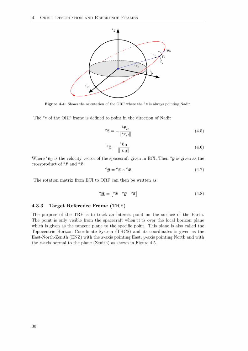
4. Orbit Description and Reference Frames
iz
iy
ix
B
oxoz
oyirB
ivB
Figure 4.4: Shows the orientation of the ORF where the oz is always pointing Nadir.
The oz of the ORF frame is defined to point in the direction of Nadir
oz = −irB‖irB‖
(4.5)
ox =ivB
‖ivB‖(4.6)
Where ivB is the velocity vector of the spacecraft given in ECI. Then oy is given as thecrossproduct of oz and ox.
oy = oz × ox (4.7)
The rotation matrix from ECI to ORF can then be written as:
oiR =
[ox oy oz
](4.8)
4.3.3 Target Reference Frame (TRF)
The purpose of the TRF is to track an interest point on the surface of the Earth.The point is only visible from the spacecraft when it is over the local horizon planewhich is given as the tangent plane to the specific point. This plane is also called theTopocentric Horizon Coordinate System (THCS) and its coordinates is given as theEast-North-Zenith (ENZ) with the x-axis pointing East, y-axis pointing North and withthe z-axis normal to the plane (Zenith) as shown in Figure 4.5.
30

4.3. Reference Frames
iz
iy
ix
B
iR∆
α
Ti (East)
j (North)
k (Zenith)
Figure 4.5: Shows the THCS given by the span ofi, y
with the vector i
R∆ pointing fromthe target (T) in the direction of the spacecraft (B).
The origin of the TRF is defined where the position vector iR∆ intersects with the
spacecraft’s CoM. The tz-axis of the TRF is the negative unit vector of the iR∆ position
vector denoted by − ir∆. The calculation of ir∆ is described in Section 6.6.
The ty-axis is given as a unit vector perpendicular to the plane spanned by the velocityvector ox and the tz. The tx-axis is then given as the cross product between tz and tyto complete the right handed Cartesian coordinate system as shown in Figure 4.6.
iz
iy
ix
BT
txtz
ty
ir
irT irB
Figure 4.6: Shows the TRF located in the CoM of the satellite body B, where the tz-axispoints to the target T and tx-axis points in the direction of flight.
31

4. Orbit Description and Reference Frames
4.3.4 Rotation Between ECI and TRF
The rotation between ECI and TRF is derived from the position vector of the satelliteand the target given in the ECI frame.
tz = −irB − irT
‖irB − irT‖(4.9)
where:
irB is the satellite position vector. [m]irT is the target position vector. [m]
(4.10)
The ty-axis is then derived from the velocity vector of the satellite given in the ORF.The ty-axis of the TRF is defined as being perpendicular to the plane spanned by thevelocity vector ivB and the tz.
ty = tz ×ivB
‖ivB‖(4.11)
where
ivB is the satellite velocity vector given in the ECI frame. [m/s]
(4.12)
The tx of the TRF is then the normal to the (ty,tz)-plane forming a right handedCartesian coordinate system.
tx = ty × tz (4.13)
4.3.5 Body Reference Frame (BRF)
The satellite BRF is defined to have its origin in CoM of the satellite. The orientation ofthe coordinate system is defined in relation to the mission of the satellite e.g. a missionpayload containing a camera would have one of the axis pointing in the direction ofthe camera. In general the BRF is defined such that the coordinate system is easilyrecognised by looking at the spacecraft.
The attitude error of a spacecraft in orbit could for example be the angular differencebetween the TRF and the BRF which is the rotation needed for pointing e.g. a cameraat a specific point on the Earth’s surface.
In this project the BRF is defined as the coordinate system shown in Figure 4.7.
32

4.3. Reference Frames
by
bzbx
Figure 4.7: Shows the CubeSat BRF which is centred in the CoM.
Rotation Between ECI and BRF
The attitude of the satellite is given by the rotation relative to the ECI. The orientationof the spacecraft is found through an ADS.
4.3.6 Control Reference Frame (CRF)
The spacecraft dynamics originates from the Control Reference Frame (CRF). The CRFis used to describe the satellites mass distribution and has its origin in the CoM of thespacecraft. All the external torques from the actuators and disturbances is described inthis reference frame. The frame originates from the satellite’s inertia matrix where theaxes are defined by the principal axes of the inertia matrix.
The cz-axis of the CRF points in the direction of the major-axis where the Momentof Inertia (MoI) is largest. The cx-axis is then defined as pointing in the directionof the minor-axis where the MoI is smallest. The cy-axis is the perpendicular to the(cx,cz)-plane so it completes the right handed Cartesian coordinate system.
Rotation Between BRF and CRF
It is possible that the CRF and the BRF have zero rotation between each other. Thiswould mean that the satellite’s mass was distributed symmetrically over the body of thesatellite, but this is not always the case. Often the CoM of the satellite is moved awayfrom the geometric centre and the principal axes of the inertia matrix is rotated becauseof uneven mass distribution.
This rotation caused by the uneven distributed mass is found by taking the EigenvalueDecomposition (EVD) of the inertia matrix and thereby finding its correspondingeigenvectors and eigenvalues as shown in equation 4.14
J = RJ′R−1 (4.14)
33

4. Orbit Description and Reference Frames
Where
J is the satellite body inertia matrix. [m]
J′ is the satellite principal moments of inertia. [m]
R is the transformation matix, with respective eigen vectors. [m]
(4.15)
4.3.7 Global Reference Frame (GRF)
The Global Reference Frame (GRF) is a reference frame used by the attitude controltestbeds attitude determination system. The purpose of the GRF is to ease themathematical derivations of the attitude estimator. The GRF is defined as an EastNorth Up (ENU) reference frame where the x-axis, gx, is pointing East, the y-axis, gy,is pointing North and the z-axis, gz is pointing up; all defined in the ECEF.
4.3.8 Summary
Through this chapter a keplerian orbit has been described together with the orbitalperturbation model, SGP4. After this a number of reference frames where defined.These reference frames will be used, through the rest of the report, in order to simplifythe mathematics. In the following chapter the models used in the design of the attitudecontrol algorithms, and in the simulations, are described.
34

Chapter 5
Spacecraft and DisturbanceModelling
In this chapter the models for the satellite are identified. These models will be used toanalyse the motion of the satellite, this includes both the kinematic and the dynamicequations. The disturbances are identified and modelled in order to take these intoaccount during the design of the control strategies. In order to be able to exert the exactnecessary torque on the satellite body, the chosen actuators, as described in Section 1.2,are modelled.
5.1 Satellite Kinematic Equation
Sources: [Sidi 97] [Wertz 95] [Markley 14]
The kinematics of a satellite are defined as the motion relative to time. Quaternionsare used as attitude representation and this means that the kinematics are the rate ofchange in attitude - the derivative of the attitude quaternion. The quaternion algebrais described in Appendix A.
The attitude quaternion q(t+∆t) at the time t+∆t can be split up into:
q(t+∆t) = q(t)⊗ q(∆t) (5.1)
Dividing the quaternion into a real and a pure quarternion part
q(∆t) = cos
(∆Φ
2
)+ u sin
(∆Φ
2
)(5.2)
Where the sine and cosine parts can be replace by the small angle approximation:
cos
(∆Φ
2
)≈ 1
sin
(∆Φ
2
)≈ 1
2ω∆t
(5.3)
Equation (5.1) and equation (5.3) can then be combined into:
q(t+∆t) ≈
I+1
2ω∆t
0 −u3 u2 u1u3 0 −u1 u2−u2 u1 0 u3−u1 −u2 −u3 0
q(t) (5.4)
35

5. Spacecraft and Disturbance Modelling
This can be simplified to:
q(t+∆t) ≈ 1
2∆t ·Ω(ω)q(t) + q(t) (5.5)
Where Ω(ω) is the four-dimensional skewsymmetric crossproduct operator
Ω(ω) =
0 −ω3(t) ω2(t) ω1(t)
ω3(t) 0 −ω1(t) ω2(t)−ω2(t) ω1(t) 0 ω3(t)−ω1(t) −ω2(t) −ω3(t) 0
(5.6)
Equation (5.5) is rearranged to
q(t+∆t)− q(t)
∆t=
1
2Ω(ω)q(t) (5.7)
If a limit is imposed the kinemateic equation appears
q(t) = lim∆t→0
q(t+∆t)− q(t)
∆t=
1
2Ω(ω)q(t) (5.8)
The kinematic equation of the satellite is now derived. This kinematic equation is usedto describe of the satellites motion relative to time. In the following section, the satelliteschange in angular momtum relative to the sum of all external torques exerted onto thesatellite body is derived.
5.2 Satellite Dynamic Equation
Sources: [Sidi 97] [Wertz 95] [Markley 14]
The dynamics of a satellite describes the rotational motion of the satellite relative tothe torques exerted, whether the torques stems from actuator torques or disturbancetorques. The rotational dynamics are derived using Euler’s rigid body dynamics.
The angular momentum can be written as:
iL(t) = J s
iω(t) (5.9)
Where ω(t) =[ω1 ω2 ω3
]> and J s is the inertia matrix of the satellite.
According to Eulers second law the applied torque can be derived as the time derivativeof the angular momentum [Serway 14]:
iτext(t) =d
dtiL(t)
=i ˙L(t)
(5.10)
Where the torque described in the control reference frame can be described as:
cτext(t) =d
dt
(ciR
iL(t)
)=
ciR
iL(t) + c
iRi ˙L(t)
(5.11)
Where the derivative of a rotation matrix can be written as [Markley 14]:ciR = − cω(t)× c
iR (5.12)
36

5.3. Disturbances
Inserted in equation (5.11) this gives:
cτext(t) = − cω(t)× ciR
iL(t) + c
iRi ˙L(t)
= − cω(t)× cL(t) +
c ˙L(t)(5.13)
Using equation (5.9) and isolating the angular acceleration, results in the satellitedynamic equation.
cτext(t) = − cω(t)× J scω(t) + J s
c ˙ω(t)
J sc ˙ω(t) = − cω(t)× J s
cω(t) + cτext(t)
c ˙ω(t) = J−1s [− cω(t)× J s
cω(t) + cτext(t)]
(5.14)
Equation (5.14) can be simplified to:
c ˙ω(t) = J−1s [−S (cω)J s
cω(t) + cτext(t)] (5.15)
where cτext is the sum of all external torques; both the actuator torques and thedisturbances. S (cω) is the three-dimensional skew-symmetric crossproduct operator,defined as:
S (ω) ,
0 −ω3 ω2
ω3 0 −ω1
−ω2 ω1 0
(5.16)
In the previous sections both the kinematics and dynamics of the satellite body, hasbeen derived. These can be used in a deterministic approach. The next step is to identifythe forces and torques the satellite will be subject to in a space environment. These aredescribed in the following sections.
5.3 Disturbances
Space is a harsh environment featuring multiple disturbances. The major disturbancestaken into account in a LEO are the residual magnetic moment, aerodynamic drag andthe radiation pressure [Wertz 95]. In the following sections these three disturbances willbe described.
5.3.1 Residual Magnetic Torque
Sources: [Wertz 95] [NASA 69b]
A satellite in orbit, travels in the geomagnetic field of the Earth. This leads to threemain magnetic disturbance torques. These are the effects of the interaction between thesatellite and geomagnetic field.
• Eddy currents• Hysteresis• Spacecraft magnetic moments
Eddy Current induces a small magnetic field in the metal. When a ferromagneticmaterial a exposed to magnetism then an electric field is induced in the material. Thiselectric field leads to small currents running in the ferromagnetic material these currentsare called eddy currents.
37

5. Spacecraft and Disturbance Modelling
Hysteresis is the phenomenon of ferromagnetic materials on a molecular level getsmagnetised by another magnet. When exposed to a magnetic field, the molecules in thematerial will align with the field and thereby rendering its own magnetic field.
Spacecraft Magnetic Moments; of the three disturbance mentioned here, this is usuallythe largest one. Spacecraft generated magnetic moment are caused by for example thewiring inside the satellite, the Printed Circuit Board (PCB) layout and everywhere else,where a current loop is present.
Eddy Currents and Hysteresis are negligible, compared to the Spacecraft MagneticMoment and in the following only the latter will be considered.
The spacecraft magnetic moment can be calculated as:
τmag = m× B (5.17)
Where:
m is the residual dipole moment of the satellite[Am2
]B is the Earth geocentric magnetic flux density
[Wb
m2
]The magnetic residual torque τmag is inherently difficult to calculate because of theuncertainty in residual dipoles direction and size which depends on the specific satellite.In [Wertz 95], the Firesat example is suggested to have a magnetic moment m of 1 Am2
for a 110W satellite. A single unit CubeSat is expected to have an average power of1W which is approximately 100 times less than the Firesat. This would give a qualifiedguesstimate of 0.01 Am2 for the satellites residual dipole moment m. The worst casemagnetic residual torque τm can then be approximated by
τm = m ·B (5.18)
where B can be approximated for a polar orbit by
B =2 ·MR3
(5.19)
where M is the magnetic moment of the Earth given as 7.96 · 1015 tesla ·m3 and R isthe radius from the centre of the Earth to the satellite where R = (6378.1 + 300) · 103[Wertz 95]. The worst case magnetic residual torque is then found by
τm = 0.01 · 2 · 7.96 · 1015
(6978100)3= 4.6852 · 10−7 [Nm] (5.20)
Which is later found to be the largest disturbance of those selected.
5.3.2 Aerodynamic Drag
Sources: [Wertz 95] [NASA 71]
In the upper atmosphere at orbital heights for a LEO, the gas particles that hit thesatellite are reflected. This creates a force on the spacecraft opposite to the direction oftravel.
38
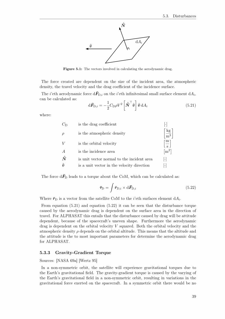
5.3. Disturbances
dAi
ˆN
ˆv
Figure 5.1: The vectors involved in calculating the aerodynamic drag.
The force created are dependent on the size of the incident area, the atmosphericdensity, the travel velocity and the drag coefficient of the incidence surface.
The i’eth aerodynamic force dFD,i on the i’eth infinitesimal small surface element dAi,can be calculated as:
dFD,i = −1
2CDρV
2
[ˆN>ˆv
]ˆv dAi (5.21)
where:
CD is the drag coefficient [·]
ρ is the atmospheric density[kg
m3
]V is the orbital velocity
[ms
]A is the incidence area
[m2
]ˆN is unit vector normal to the incident area [·]ˆv is a unit vector in the velocity direction [·]
The force dFD leads to a torque about the CoM, which can be calculated as:
τD =
∫rD,i × dFD,i (5.22)
Where rD is a vector from the satellite CoM to the i’eth surfaces element dAi.
From equation (5.21) and equation (5.22) it can be seen that the disturbance torquecaused by the aerodynamic drag is dependent on the surface area in the direction oftravel. For ALPHASAT this entails that the disturbance caused by drag will be attitudedependent, because of the spacecraft’s uneven shape. Furthermore the aerodynamicdrag is dependent on the orbital velocity V squared. Both the orbital velocity and theatmospheric density ρ depends on the orbital altitude. This means that the altitude andthe attitude is the to most important parameters for determine the aerodynamic dragfor ALPHASAT.
5.3.3 Gravity-Gradient Torque
Sources: [NASA 69a] [Wertz 95]
In a non-symmetric orbit, the satellite will experience gravitational torques due tothe Earth’s gravitational field. The gravity-gradient torque is caused by the varying ofthe Earth’s gravitational field in a non-symmetric orbit, resulting in variations in thegravitational force exerted on the spacecraft. In a symmetric orbit there would be no
39
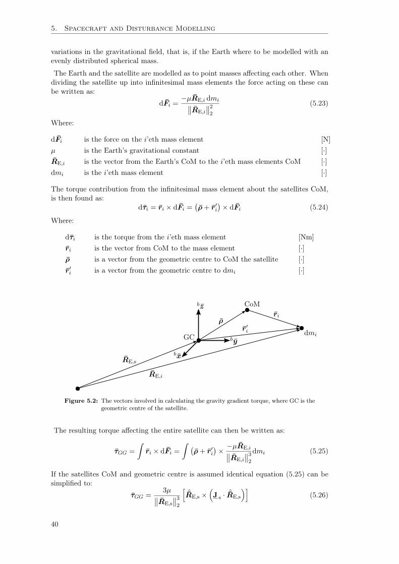
5. Spacecraft and Disturbance Modelling
variations in the gravitational field, that is, if the Earth where to be modelled with anevenly distributed spherical mass.
The Earth and the satellite are modelled as to point masses affecting each other. Whendividing the satellite up into infinitesimal mass elements the force acting on these canbe written as:
dFi =−µRE,i dmi∥∥RE,i
∥∥22
(5.23)
Where:
dFi is the force on the i’eth mass element [N]
µ is the Earth’s gravitational constant [·]RE,i is the vector from the Earth’s CoM to the i’eth mass elements CoM [·]dmi is the i’eth mass element [·]
The torque contribution from the infinitesimal mass element about the satellites CoM,is then found as:
dτi = ri × dFi =(ρ+ r′i
)× dFi (5.24)
Where:
dτi is the torque from the i’eth mass element [Nm]
ri is the vector from CoM to the mass element [·]ρ is a vector from the geometric centre to CoM the satellite [·]r′i is a vector from the geometric centre to dmi [·]
dmi
CoM
RE,s
GC
RE,i
ρri
r′i
bz
by
bx
Figure 5.2: The vectors involved in calculating the gravity gradient torque, where GC is thegeometric centre of the satellite.
The resulting torque affecting the entire satellite can then be written as:
τGG =
∫ri × dFi =
∫ (ρ+ r′i
)×
−µRE,i∥∥RE,i
∥∥32
dmi (5.25)
If the satellites CoM and geometric centre is assumed identical equation (5.25) can besimplified to:
τGG =3µ∥∥RE,s
∥∥32
[ˆRE,s ×
(J s · ˆRE,s
)](5.26)
40
5.3. Disturbances
Where:
J s is the moment of inertial tensor of the satellite [·]RE,s is the vector from the Earth’s CoM to the satellite CoM [·]
From equation (5.26) it can be seen that it produces a vector which the gravity gradienttorque is about, and a scaling of that vector which depends on the distance to the Earth’scentre.
If a spacecraft is in an elliptical orbit then the gravity gradient would vary over thecoarse of the orbit; caused by the varying of the distance to the centre of the Earth.The gravity gradient torque also depends on the mass distribution of the spacecraftas the cross product is between ˆRE,s and J s
ˆRE,s where the latter is a perturbationcaused by the spacecraft’s moment of inertia tensor. If the spacecraft had a perfectevenly distributed moment of inertia then there would be no torque disturbance fromthe gravity gradient.
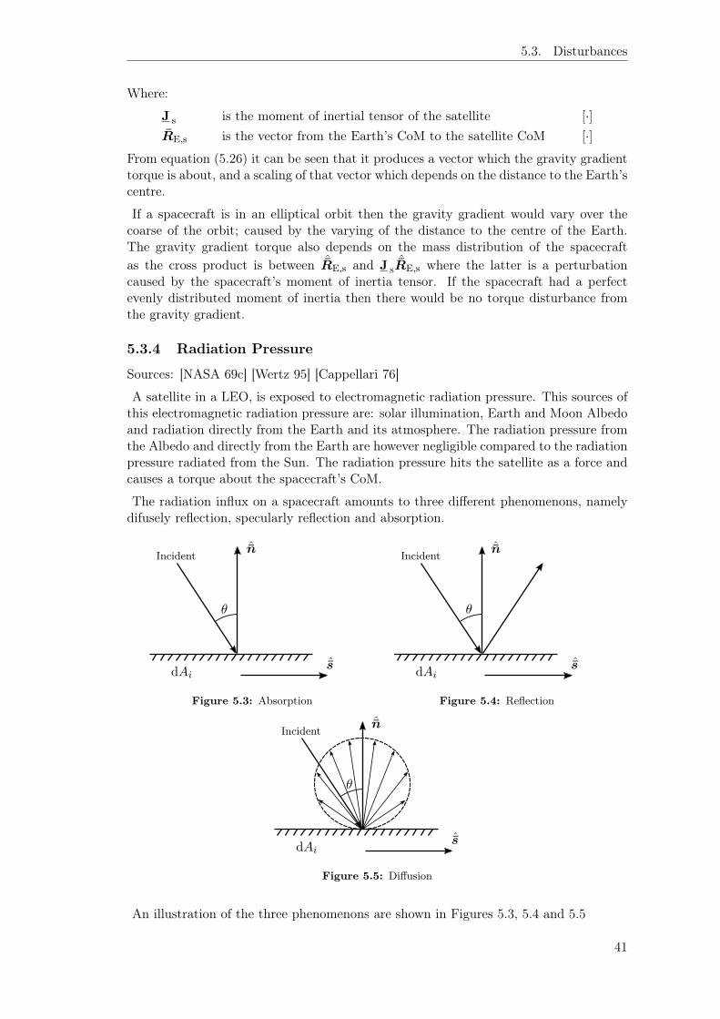
5.3.4 Radiation Pressure
Sources: [NASA 69c] [Wertz 95] [Cappellari 76]
A satellite in a LEO, is exposed to electromagnetic radiation pressure. This sources ofthis electromagnetic radiation pressure are: solar illumination, Earth and Moon Albedoand radiation directly from the Earth and its atmosphere. The radiation pressure fromthe Albedo and directly from the Earth are however negligible compared to the radiationpressure radiated from the Sun. The radiation pressure hits the satellite as a force andcauses a torque about the spacecraft’s CoM.
The radiation influx on a spacecraft amounts to three different phenomenons, namelydifusely reflection, specularly reflection and absorption.
ˆn
θ
dAiˆs
Incident
Figure 5.3: Absorption
ˆn
θ
dAiˆs
Incident
Figure 5.4: Reflection
ˆn
θ
dAiˆs
Incident
Figure 5.5: Diffusion
An illustration of the three phenomenons are shown in Figures 5.3, 5.4 and 5.5
41
5. Spacecraft and Disturbance Modelling
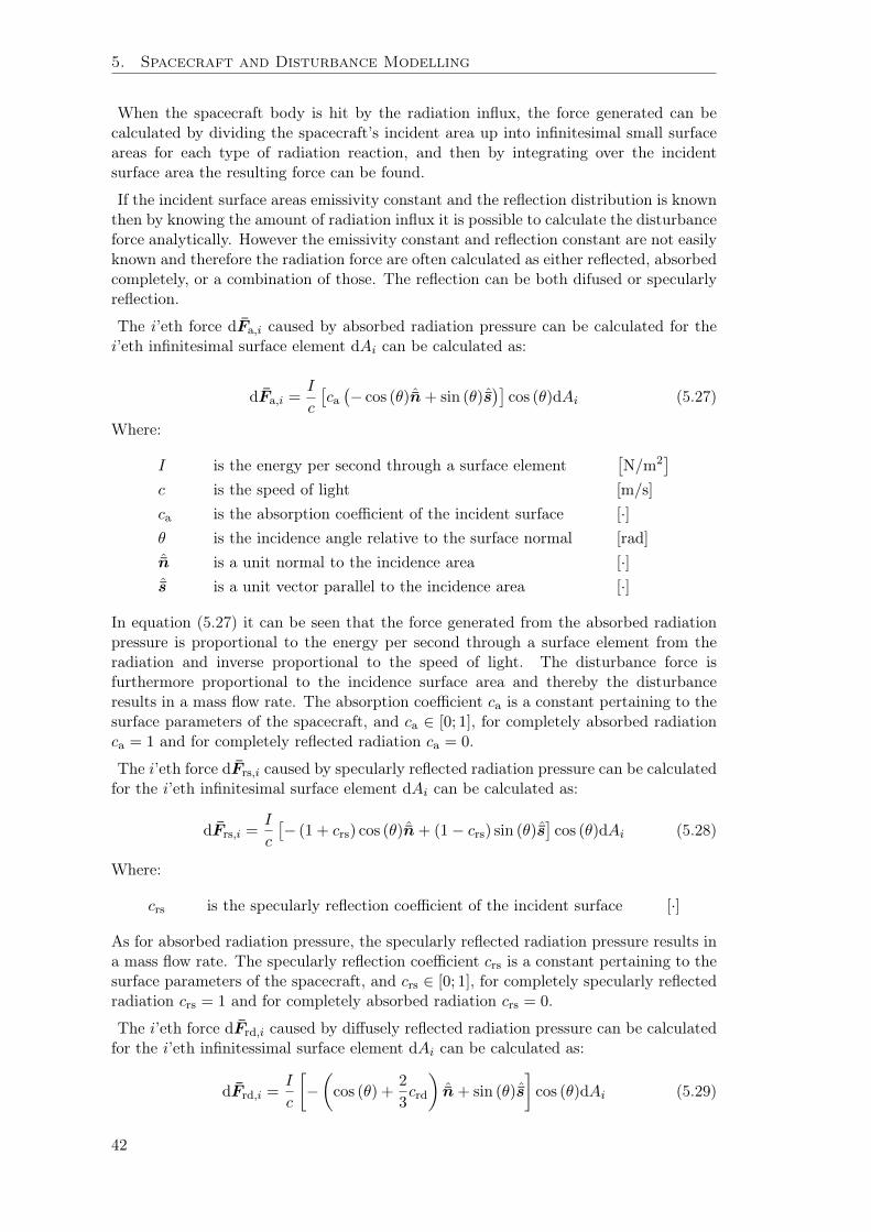
When the spacecraft body is hit by the radiation influx, the force generated can becalculated by dividing the spacecraft’s incident area up into infinitesimal small surfaceareas for each type of radiation reaction, and then by integrating over the incidentsurface area the resulting force can be found.
If the incident surface areas emissivity constant and the reflection distribution is knownthen by knowing the amount of radiation influx it is possible to calculate the disturbanceforce analytically. However the emissivity constant and reflection constant are not easilyknown and therefore the radiation force are often calculated as either reflected, absorbedcompletely, or a combination of those. The reflection can be both difused or specularlyreflection.
The i’eth force dFa,i caused by absorbed radiation pressure can be calculated for thei’eth infinitesimal surface element dAi can be calculated as:
dFa,i =I
c
[ca
(− cos (θ) ˆn+ sin (θ)ˆs
)]cos (θ)dAi (5.27)
Where:
I is the energy per second through a surface element[N/m2
]c is the speed of light [m/s]
ca is the absorption coefficient of the incident surface [·]θ is the incidence angle relative to the surface normal [rad]
ˆn is a unit normal to the incidence area [·]ˆs is a unit vector parallel to the incidence area [·]
In equation (5.27) it can be seen that the force generated from the absorbed radiationpressure is proportional to the energy per second through a surface element from theradiation and inverse proportional to the speed of light. The disturbance force isfurthermore proportional to the incidence surface area and thereby the disturbanceresults in a mass flow rate. The absorption coefficient ca is a constant pertaining to thesurface parameters of the spacecraft, and ca ∈ [0; 1], for completely absorbed radiationca = 1 and for completely reflected radiation ca = 0.
The i’eth force dFrs,i caused by specularly reflected radiation pressure can be calculatedfor the i’eth infinitesimal surface element dAi can be calculated as:
dFrs,i =I
c
[− (1 + crs) cos (θ) ˆn+ (1− crs) sin (θ)ˆs
]cos (θ)dAi (5.28)
Where:
crs is the specularly reflection coefficient of the incident surface [·]
As for absorbed radiation pressure, the specularly reflected radiation pressure results ina mass flow rate. The specularly reflection coefficient crs is a constant pertaining to thesurface parameters of the spacecraft, and crs ∈ [0; 1], for completely specularly reflectedradiation crs = 1 and for completely absorbed radiation crs = 0.
The i’eth force dFrd,i caused by diffusely reflected radiation pressure can be calculatedfor the i’eth infinitessimal surface element dAi can be calculated as:
dFrd,i =I
c
[−(cos (θ) +
2
3crd
)ˆn+ sin (θ)ˆs
]cos (θ)dAi (5.29)
42
5.4. Actuator Models
Where:
crd is the diffusely reflected coefficient of the incident surface [·]
As for both the absorbed radiation pressure and the specularly reflected radiationpressure, the difusely reflected radiation pressure results in a mass flow rate. Thediffusely reflection coefficient crd is a constant pertaining to the surface parameters ofthe spacecraft, and crd ∈ [0; 1], for completely diffusely reflected radiation crd = 1 andfor no diffusely reflected radiation pressure crd = 0.
The absorption coefficient, specularly reflection coefficient and the diffusely reflectioncoefficient must comply with:
ca + crs + crd ∈ [0; 1] (5.30)
The torque about CoM stemming from radiation pressure can then be found as:
τr =N∑i=0
[rrs,i × dFrs,i + ra,i × dFa,i + rrd,i × dFrd,i
](5.31)
Where:
rrs,i, rrd,i & ra,i is vectors from CoM to the i’eth surface element [·]for each of the three types of radiation pressure
From Equations 5.27, 5.28 and 5.29 it can be seen that the magnitude of radiationpressure depends primarily on the attitude of the spacecraft and the surface materialimpacted. The attitude of the spacecraft is the parameter, which determines the size ofthe surface area impacted by the radiation, and the surface material determines if theradiation pressure is caused by difusely reflection, specularly reflection or absorption.
5.4 Actuator Models
As shown in section 5.3 the satellite experience different types of disturbances whenin orbit. These disturbance torques will quickly reorientate the spacecraft unless itgenerates an equally large torque to counter the disturbances. This is a job for theADCS, which in this thesis is equipped with reaction wheels to acquire disturbancerejection and active attitude control by generating corrective torques on the satellitebody. The model of the reaction wheels will be described through out this section.
5.4.1 Reaction wheel
Source: [Sidi 97] [Franklin 10]
Euler’s moment equations states that, any external torques acting on the rigid bodytranslates to the angular momentum of the spacecraft. Active attitude control isaccomplished by translating mechanical momentum to the principal axis of the rigidbody of the spacecraft, by use of reaction wheels.
A three wheeled configuration, where each reaction wheel is placed parallel to a principalaxis of the body, simplifies the control problem e.g. by having direct translation ofmoment between reaction wheel momentum and the spacecraft principal axes. Thisactuator configuration has no redundancy and looses controllability if an actuator isdamaged. This reason justifies the use of a fourth reaction wheel where the configurationof these will be described in the following sections.
43
5. Spacecraft and Disturbance Modelling
An ACS with four actuators can be described as an over-actuated control system forwhich presents the problem of allocating the control signal over all four actuators. Thistopic will be described in the Control Allocation section. First a dynamic model of themotors generating the torque is described.
Dynamic Model
Source: [Xia 12]
The reaction wheels momentum is generated by four BLDCs. Compared to a traditionalDC Motor (DC), the BLDC windings is energised dependant on the rotor positionand controlled by a three-phased signal. For each phase the winding is conducted theelectromagnetic torque and back-EMF is the same as for a DC motor. This means thatthe same models for a DC motor can be used when modelling a BLDC motor.
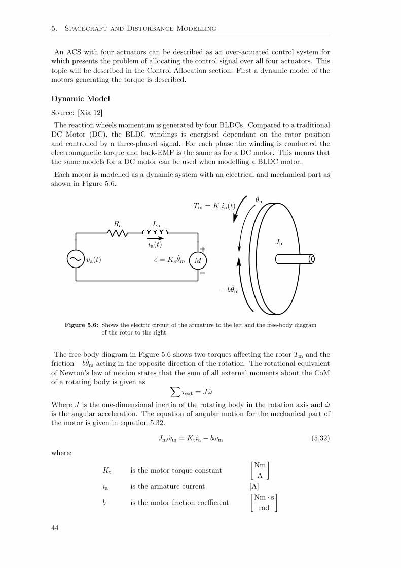
Each motor is modelled as a dynamic system with an electrical and mechanical part asshown in Figure 5.6.
va(t) e = Keθm
Ra La
ia(t)
Tm = Ktia(t)θm
−bθm
Jm
M
Figure 5.6: Shows the electric circuit of the armature to the left and the free-body diagramof the rotor to the right.
The free-body diagram in Figure 5.6 shows two torques affecting the rotor Tm and thefriction −bθm acting in the opposite direction of the rotation. The rotational equivalentof Newton’s law of motion states that the sum of all external moments about the CoMof a rotating body is given as ∑
τext = Jω
Where J is the one-dimensional inertia of the rotating body in the rotation axis and ωis the angular acceleration. The equation of angular motion for the mechanical part ofthe motor is given in equation 5.32.
Jmωm = Ktia − bωm (5.32)
where:
Kt is the motor torque constant[Nm
A
]ia is the armature current [A]
b is the motor friction coefficient[Nm · srad
]
44

5.4. Actuator Models
The electrical part of the motor is given as shown in Figure 5.6 is given as a RL circuitand modelled as in equation
Lad
dtia(t) +Raia(t) = va(t)−Keωm (5.33)
where:
La is the armature self inductance [H]
Ra is the armature electrical resistance [Ω]
va is the armature voltage [V]
Ke is the motor friction coefficient[V · srad
]where for a BLDC the current running through the windings is controlled by the three-phases generated by the motor driver. Each phase is separated by a 120 [deg] whichmeans that there will effectively only be running current in two of the windings meaningthat the motor coefficients should be measured from phase to phase.
The dynamics of the electrical circuit induction relative to the dynamics of themechanical motion is often said to have negligible effect and is therefore neglected.The combination of equation of motion from equation 5.32 and electrical dynamics fromequation 5.33 is then given as equation 5.34.
Jmωm = −(KtKe
Ra+ b
)ωm +
Kt
Rava(t) (5.34)
As seen from equation 5.34, Jmωm = τm which is the sum of all torques on the motorshaft. Then it is known from Newton’s third law of motion that for every action thereis an equally large reaction and in the case of a rotating body the action exerted on themotor shaft is the motor torque τm which has an equally large reaction −τm acting onthe mount on which the motor is mounted in the satellite rig.
The reaction torque −τm is directly translated to the satellite body if the motor ispointing in the direction of the principal axis of the body. To suppress disturbancetorques and reorientate the satellite, the reaction torque generated by the motors mustbe large enough. This is accomplished by increasing the inertia on the motor shaft.As seen from equation 5.34, the torque is directly dependent on the inertia Jm and theangular acceleration ωm.
τrw = −(Jw + Jm)ωm (5.35)
where τrw is the reaction torque acting on the satellite body and Jw is the inertia ofthe reaction wheel. Since Jw Jm the shaft inertia Jm is neglected. The dimensioningof the reaction wheels is also dependent on the number of actuators used and theirconfiguration.
Reaction Wheel Configuration
As described in the introduction, the use of four reaction wheels increases the reliabilityof the ACS by having redundancy if one motor fails. The configuration of these reactionwheels should be orientated such that the moment generated by each reaction wheel hasa torque components in at least two of the three principal axis of the satellite body.
The ALPHASAT attitude control is equipped with four reaction wheels in aTetrahedron configuration. This is due to the fact that the Tetrahedron configuration has
45

5. Spacecraft and Disturbance Modelling
redundancy and the capability of zero angular momentum transition. The configurationis also capable of performing twice the maximum torque of a reaction wheel on a singleaxis.
All the reaction wheels in the tetrahedron configuration is orientated such that allangular momentums cancel out each other, when running with the same biased angularvelocity. The distribution of the angular moments of the reaction wheels τi, i ∈ [1; 4]is projected onto the tree-dimensional control space by the distribution matrix Pw asshown in equation 5.36.
τcxτcyτcz
= Pw
τ1τ2τ3τ4
(5.36)
where Pw is the Tetrahedron configurations distribution matrix which is defined tohave a row sum of zero, which means that all torques generated by the reaction wheelswill chancel out each other when running at same biased angular velocity and is givenby:
Pw =
cosβ − cosβ cosα − cosβ cosα 00 cosβ cos α
2 − cosβ cos α2 0
− sinβ − sinβ − sinβ 1
(5.37)
-22
-1.5-1
-0.5
1 2
0z
0.5
1
1
y
0
1.5
x
0
2
-1 -1-2 -2
Local Reference FrameRW Torque ProjectionRW1RW2RW3RW4
Figure 5.7: Shows direction of each reaction wheel in the tetrahedron configuration.
The τc vector is calculated from the control laws. Since the there are four reactionthe system is said to be over-actuated which means that there exists infinite solutionsto the torque component τi. This is seen from the distribution matrix Pw which is anunder-determined system.
46

5.4. Actuator Models
Control Allocation
In order to find a solution to an over-actuated system given as.τ1τ2τ3τ4
= P+w
τcxτcyτcz
(5.38)
where P+w is a right Moore-Penrose pseudo-inverse matrix. The right pseudo-inverse of
a under-determined system can be found as:
A+ = A>(AA>
)−1(5.39)
where A+ is the minimum norm solution to the over-actuated system, which means thatthe control torque will be distributed evenly amongst all four reaction wheels. Then thelinear-map from the control torque τc given in the CRF to a desired reaction wheeltorque is given as.
wτ = P+w
cτ c (5.40)
Which means that from now on, when ever a control value has been calculated, thereexists a linear combination that maps the tree-dimensional control torque to the four-dimensional reaction wheel torque by the use of the Moore-Penrose pseudo-inversematrix.
5.4.2 Dynamic Model of Reaction Wheel Configuration
The dynamic equations of reaction wheels mounted in the satellite frame is described byEuler’s second law which states that a change in angular momentum
i ˙L(t) in an inertialreference frame is equal to the sum of all external forces τext acting on a rigid body,given as:
iτ ext =d
dtiL(t)
=i ˙L(t)
(5.41)
Where as the change in angular momentum of a single reaction wheel is given as therotation of the angular momentum between ECI and one Reaction Wheel ReferenceFrame (RWRF) and is given by multiplication of the rotation matrix w
iR
wτ ext(t) =d
dt
(wiR
iL(t)
)=
wiR
iL(t) + w
iRi ˙L(t)
(5.42)
where the derivative of the rotation matrix is expressed as the product between theskew-symmetric cross product operator defined in equation 5.16 and the rotation matrixfrom ECI to RWRF.
wiR = −S (wω)wiR (5.43)
Using the rotational derivative expressed by equation 5.43 in equation 5.42 the followingis seen.
wτ ext(t) = −S (wω(t))wiRiL(t) + w
iRi ˙L(t)
= −S (wω(t))wL(t) +
w ˙L(t)(5.44)
47

5. Spacecraft and Disturbance Modelling
Further from this is can be seen that the change of angular momentum of a reactionwheel mounted in the satellite body is equal to the sum of the Coriolis force and theexternal forces.
w ˙L(t) = −S (wω(t))wL(t) + wτ ext(t) (5.45)
where wτ ext(t) is the torque generated by the BLDC motor and wω is the sum of therotational velocity of the satellite in RWRF and the reaction wheel given as.
wω(t) = wωs(t) +wωw(t) (5.46)
where wωs(t) = [wωsxwωsy
wωsz]> and wωw(t) = [0 0 wωwz]
>.
The change in angular momentumw ˙L(t) is now described for one wheel in the RWRF.
The torque from the reaction wheel is described in RWRF and is translated to the CRFwhere the MoI of the satellite is defined. Therefore the change in angular momentumin the CRF caused by the reaction wheel is described as:
c ˙Lw(t) = − cwR
w ˙Lw(t) (5.47)
The sign change of the torque exerted on the CRF is explained by Newtons third law ofmotion, that states, for every action acting on a rigid body there exists an equally largeopposite reaction, which also applies for rotational bodies. This implies that the changein angular momentum on the reaction wheel has an opposite effect on the satellite CRF.The rotational dynamics described in equation 5.45 is only accompanying one reactionwheel. The total change in angular momentum is then given as the sum of all momentsgenerated by the reaction wheels. It should be noted that for every reaction wheel, aunique rotation matrix exists and is denoted by i ∈ [1; 4]
c ˙Lth(t) = −4∑
i=1
c ˙Lw,i(t) (5.48)
The resulting change in angular momentumc ˙Lth(t) is then added to the external torques
in the dynamic model of the satellite given in Section 5.2.
5.5 Summary
Now the models for both the satellite kinematics, dynamics and the actuator model butalso the disturbance torques, a spacecraft can expect to meet in a space environment, hasbeen presented. The satellite kinematics and dynamics will be used in simulations of thesatellite in order to describe the spacecraft’s behaviour both in terms of time and exertedtorques and forces. The disturbance models are used to model the space environmentduring the simulations, and the actuator models are used for both simulating thespacecraft behaviour but also in the design of the attitude control algorithms. In thefollowing chapter the simulation environment is described.
48

Chapter 6
Simulation Environment
Through the previous chapters, knowledge of the satellite model and its orientationin orbit, how it is propagated over time and disturbances is gained through analysis.In order to simulate the control algorithms, a simulation environment is built. Theenvironment enables the possibilities to simulate weightlessness, vacuum and thedisturbances in a space environment.
Through this Chapter, the elements of the simulation environment is described. Firstan outline of the simulation environment is described and then a short description ofthe simulation blocks used.
6.1 Simulink Implementation
The purpose of the simulation environment is for verification and performance test ofboth the linear and non-linear regulator designed in the Sections 7.1 and 7.2. The scopeof this project is not to design attitude determination, but to investigate regulator designfor CubeSats. The basic structure of the simulation environment is illustrated in Figure6.1.
Disturbances
irs
bqs
bωs
SpacecraftDynamics
&Orbit Probagation
b ˙Ld
b ˙Lc
tinit
bqs,init
TLE
ControllerActuator Reference
ivs
Figure 6.1: Shows the structure of the simulation environment, where the all the systemmodels for spacecraft dynamics and orbit propagation is collected in a singledynamic block.
49

6. Simulation Environment
The system block illustrated in Figure 6.1, includes the spacecraft dynamics given bythe models obtained in Sections 5.1 and 5.2, which is a function of external torques andinitial conditions, where:
b ˙Lc is the control torque from the actuatorsb ˙Ld is the disturbance torquesbqs,init is the initial attitude of the satellite
The satellite orbit propagation model is based on the SGP4 model which estimates theposition vector irs and velocity vector ivs of a spacecraft where:
TLE is the Two Line Element, which contains the orbit parameterstinit is the initial simulation time, given in Julian Date (JD)
The outputs of the dynamic system block is then used to calculate the expecteddisturbances which depends on the orbital elements and the current attitude of thespacecraft. The output is further used in the regulator to calculate the desired controlsignal and following a given attitude reference.
6.2 The AAUSAT Library
The environment is built in Matlab/Simulink, where the AAUSAT library is defined.The simulation environment build for the ALPHASAT is based on a few selected buildingblocks used for AAUSAT3 by [Jensen 10].
The AAUSAT library contains reusable building blocks for simulating LEO andthe corresponding environmental disturbances found in space. The library has beendeveloped over the past decade by former student groups through the campaigns ofAAUSAT-II and AAUSAT3. The following building blocks from the library have beenused:
• Disturbance models• Ephemeris models• SGP4 model
The disturbance models is built on the same principles as described in Section 5.3. Thecomplete model of the satellite dynamics, orbit propagation and external torques isshown in Figure 6.2.
50

6.2. The AAUSAT Library
w_init_S
q_init_I_S
q_S_C
inertia_C
1
N_ext(S)
q_I_S
Satellite Attitude
Omega_S
Satellite angular velocity
2
TLE
init_jd
Time t(JD)
Moon position R_m(I)
Sun Position R_s(I)
Earth Rotation q(I->E)
Ephemeris
sim_time_JD
[sim_time_JD]
S_I_POS
S_I_VEL
q_I_Earth
Initial angular velocity W_i(S)
Initial attitude q(I->S)
Controller frame q(S->C)
Satellite Inertia I(C)
N_mt(S)
Disturbance N_dist(S)
Attitude q(I->S)
Angular velocity W(S)
Spacecraft Dynamics (Alphasat)
[N_dist]
[R_sun]
[R_moon]
[R_moon]
[R_sun]
[q_I_S]
[S_I_VEL]
q_S_C
sc_mass
r_com
[S_I_POS]
inertia_C
enable_env_disturbance
[N_dist]
Initial time ti(JD)
TLE
Spacecraft velocity V (I)
Spacecraft position R (I)
Simulation time t(JD)
Orbit model
Attitude q(I -> S)
Orbit velocity V_sc(I)
Orbit position R_sc(I)
R_CoM(S)
Moon positon R_m(I)
Inertia I_f(C)
Mass of Spacecraft
q(S->C)
Sun position R_s(I)
N_dist(S)
F_dist(S)
Enviroment Disturbance
[q_I_Earth]
Figure 6.2: Shows the environment blocks of the ALPHASAT, with the spacecraft dynamics,orbit models and the disturbances seen from the spacecraft.
This thesis has contributed to this library by developing:
• Satellite system models• Tetrahedron actuator model• Attitude Estimator Emulator• Target reference system• Animation environment
The target reference system is designed to simulate the case where the satellite is trackingmultiple ground stations during orbit. Furthermore, an animation environment has beendeveloped, in order to intuitively illustrate attitude manoeuvres during orbit simulations.A Preview of the 3D animation environment is shown in Figure 6.3.
51

6. Simulation Environment
Figure 6.3: Shows the Simulink 3D animation environment designed for intuitive illustratingsatellite attitude manoeuvres.
6.3 Spacecraft Dynamics Model
The satellite model block is built of a kinematic and dynamic block. The input attitude,angular velocity and external torques is given in BRF. These are then rotated to thesatellite CRF where the inertia matrix is diagonal. This rotation simplifies the equations.External torques and the initial angular velocity is then fed to the “scdynamics” blockwhere the satellite dynamic is defined as shown in Figure 6.4.
2AngularvelocityW(b)
1Attitudeq_i_b
q q^-1
6DisturbanceN_dist(b)
5N_mt(b)
4SatelliteInertiaI(c)
3Controllerframeq(b->c)
2Initialattitudeq(b)
1InitialangularvelocityW_i(b)
Initialomega_c
tau_ext
Js
omega_c
scdynamics
q_c_init
omega_cq
sckinematics
qmul
q
Vq'Vq
q
Vq'Vq
q
Vq'Vq
qmul
Figure 6.4: Shows to Simulink block of the spacecraft system model.
The “sckinematics” block uses the initial attitude quaternion to extrapolate the changein attitude given an estimated angular velocity from the satellite dynamics block. The“sckinematisc” block is based on the kinematic equation 6.1.
cqs =1
2Ω (cωs)
cqs (6.1)
The output quaternion of the kinematic block is then rotated back to the satellite BRF.
The “scdynamics” is shown in Figure 6.5 where the sum of all external torques actingon the satellite CRF is integrated to find the resulting angular velocity. The angularvelocity is then used to find the corresponding Coriolis torque acting on the satelliteCRF.
52
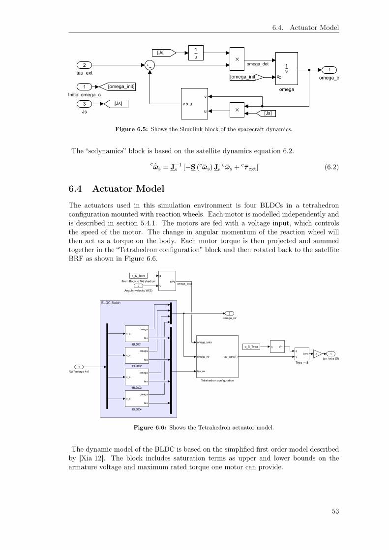
6.4. Actuator Model
1
omega_c
1
Initial omega_c
2
tau_ext
3
Js
1s
xo
omega[omega_init]
[omega_init]
v
u
v x u[Js]
[Js]
1
u[Js]
omega_dot
Figure 6.5: Shows the Simulink block of the spacecraft dynamics.
The “scdynamics” block is based on the satellite dynamics equation 6.2.
c ˙ωs = J−1s [−S (cωs)Js
cωs +cτ ext] (6.2)
6.4 Actuator Model
The actuators used in this simulation environment is four BLDCs in a tetrahedronconfiguration mounted with reaction wheels. Each motor is modelled independently andis described in section 5.4.1. The motors are fed with a voltage input, which controlsthe speed of the motor. The change in angular momentum of the reaction wheel willthen act as a torque on the body. Each motor torque is then projected and summedtogether in the “Tetrahedron configuration” block and then rotated back to the satelliteBRF as shown in Figure 6.6.
BLDCBatch
1tau_tetra(S)
1RWVoltage4x1
q_S_Tetra
FromBodytoTetrahedron2
AngularvelocityW(S)
q
Vq'Vq
omega_tetra
omega_rw
tau_rw
tau_tetra(T)
Tetrahedronconfiguration
q
Vq'Vq
Tetra->S
q_S_Tetra q q^-1
2omega_rw
v_aomega
tau
BLDC1
-1v_aomega
tau
BLDC2
v_aomega
tau
BLDC3
v_aomega
tau
BLDC4
omega_tetra
Figure 6.6: Shows the Tetrahedron actuator model.
The dynamic model of the BLDC is based on the simplified first-order model describedby [Xia 12]. The block includes saturation terms as upper and lower bounds on thearmature voltage and maximum rated torque one motor can provide.
53

6. Simulation Environment
1s Kt/Ra KeKt/Ra
b
Friction
-K-
1/Jw
1v_a
1omega
2tau
VoltageSat torquesatomega
Figure 6.7: Shows the model of a simplified BLDC.
6.5 Attitude Estimator Emulator
In order to simulate the feedback from an attitude estimator, with its given uncertaintieson the estimated states, an attitude estimator emulator has been build as shown in Figure6.8.
1q_i_s
2omega_s
3omega_rw
randomangel
noise1
vector
angleq
quaternioncomposition
q1
q2q_res
Rotationofq1byq2D2R
DegreestoRadians
noise2
randomvector1
q_b_est
2omega_b_est
3omega_rw_est
Figure 6.8: Shows the block which should emulate the uncertainties and noise from whichis propagated through an estimator.
The function of the emulator is to add noise to the feedback from the deterministicmodel so that the feedback imitates the specifications of an attitude estimator, resultingin the property to test the robustness of the regulator design.
The size of the noise term summed on the attitude bqs and the angular velocity bωs ofthe spacecraft follows the attitude estimator requirements specified by [Jensen 10]. Thisresults in an estimated attitude within ±5 [deg] and a sample rate of 1 Hz.
6.6 Target Reference Generator
Source: [Curtis 05]
The reference generator is designed in order to simulate a logic component on thespacecraft, which should choose a target reference from a list of interest points. Thisblock uses an estimate of the rotation of the ECEF and the satellites positions vectorirs to calculate which interest points on the Earth’s surface is in line of sight and thenchoose the one closet to the spacecraft.
54

6.6. Target Reference Generator
1
Simulation time t [JD]
2
POS_SC_I
t(JD) q(I->E)
ECI->ECEF quaternion
q q^-1
1
q_i_t
q_e_i
POS_SC_I
target_name
R_target_e
Get target reference
Vel_SC_I
Pos_SC_I
q_I_O
omega_o_ref
Orbit reference frame
3
Vel_SC_I
v v_hat
z_t
v
uv x u
y_t
v
uv x u
x_t
InterpretedMATLAB Fcn
DCM2Q
2
omega_t
target_name
target_name
enabel_tracking
q_i_o
omega_o
q_i_t
omega_t
q_ref
omega_ref
reference switch
[q_i_t]
[omega_t]
q_i_o
[omega_o]
[target_name]
[q_i_o]
[omega_o]
[q_i_t]
[omega_t]
enabel_target
r
v
omega
find omega_ref
target
q
Vq'Vq
v v_hat
-1
v v_hat
v v_hat
Figure 6.9: Shows the Tetrahedron actuator model.
The block “Get target Reference” generates a set of position vectors iRt,i where
i = [0, . . . , n] and n is the number of interest points in the “target_list” shown below:
%% Define targets in the format name, [lat,lon,alt]2 targets = ’Aalborg HQ’, [57.013835, 9.987509,15];
’Thule Air Base’ [76.5322, -68.0731, 500];4 ’Paderborn’ [51.5334, 8.8725, 10]
’Vienna’, [48.206251, 16.373879, 542];6 ’Lisboa’, [38.718298, -9.142485, 200];
’Sao Paulo’ [-2.000000, -44.600000,10];8 ;
save(’target_list.mat’,’targets’);
From the spherical coordinates given by the latitude and longitude, a unit vector pointingin the direction of the target can be found as shown in equation 6.3. This vector is fixedin the ECEF.
ert,i =
cos(θlat,i) cos(θlon,i)cos(θlat,i) sin(θlon,i)
sin(θlat,i)
(6.3)
The position vector is then given by the unit vector multiplied with scalar sum of theEarth’s radius and the altitude of the target from sea level. The position vector is givenby equation 6.4.
eRt,i = (Ralt,i +Re)
ert,i (6.4)
The position vector is then rotated into the ECI by the inverse rotation found in Section4.3.1. The reason for this rotation is because the Spacecraft position vector is given inthe ECI.
iRt,i =
ieq
∗ eRt,i
ieq (6.5)
Now that the target position vector is represented in ECI, it is possible to take thedifference between the two vectors in order to find a vector pointing from the spacecraftto the target as shown in equation 6.6.
iR∆,i =
iRs −
iRt,i (6.6)
55

6. Simulation Environment
When the satellite is in line of sight, it is said to be over the THCS which is explained insection 4.3.3. This is true if the angle between the two position vectors |αi| < 90 [deg].
αi = cos−1
iR>
∆,iiRt,i∥∥∥iR∆,i
∥∥∥∥∥∥iRt,i
∥∥∥ (6.7)
Depending on the surroundings of the target or groundstation, a minimum elevation canbe set, which is then subtracted from the ±90 [deg] threshold. This means that the “Gettarget reference” block only triggers on targets which is below |90− αmin| [deg]. This isalso illustrated in Figure 6.10.
iRs
iRt,i
αi
αmin
SC
Ti
iR∆,i
iy
iz
ix
THCS
Figure 6.10: Shows the satellite and one specific target Ti where αi is the inclination of thesatellite over the THCS.
As indicated by the notation, this calculation is performed for each interest point inthe list which means that more targets could potentially be in line of sight. In that case,the algorithm chooses the target closest to the satellite.
When a target has been selected, the difference vector iR∆,I pointing from the
spacecraft to the target is used to find the TRF explained in 4.3.3. In cases whereno targets is in line of sight, the target reference generator will use the Nadir referenceframe.
6.7 Simulation Setup
The simulation environment for ALPHASAT, as described, enables spacecraft simulationin a theoretical space environment with a selection of worst case disturbances a satellitewill endure in space. Through this Section, the setup used for evaluating the controllersdeveloped in Chapter 7 is described.
As mentioned in the Introduction and Mission Section 1.1, the hypothetical satelliteALPHASAT is launched into orbit from the ISS by an arbitrary deployer. This type oflaunch will give the satellite approximately the same orbital parameters as the ISS, butwill change over time due to the difference in mass and surface area compared to theISS.
When launched from the deployer, the satellite may experience tumbling, sometimeswith a greater effect, but this is expected. This can be due to skewness in the inhibit
56

6.7. Simulation Setup
switches in the bottom of the CubeSat which is the only contact area between theCubeSat and the deployer. The expected tumble rate that the CubeSat can experienceis approximately 10 deg/s. A De-tumble algorithm will then dampen the initial spin ofthe satellite down to below ±0.3 deg/s [Jensen 10]. The conditions after the detumblinghas occurred is defined as the initial conditions for attitude control algorithms testedwith the simulation.
Simulation Specifications
In the following section, a list of the simulation conditions is specified. First thesimulation time which is used to determine the satellites position in the given orbit.
t_sim = ’2015-10-20T14:35Z’
Second the following TLE is used for simulating the ALPHASAT orbit given an ISSlaunch.
ALPHASAT1 40949U 98067HA 16131.17243197 .00049328 00000-0 32059-3 0 99902 40949 51.6335 230.6137 0003739 51.3487 308.7846 15.75443623 34062
Given the initial simulation time and the TLE, the CubeSat is at an altitude ofapproximately 379 Km and flying over the Atlantic ocean in direction of the Germanywhere a ground station is positioned.
6.7.1 Simulation Scenarios
The ALPHASAT will be simulated in two scenarios where the each controller is verified.The initial values is the same for both controllers in each simulation for comparison.The scenarios are:
• Nadir PointingIn this scenario, the satellite is initialised, as mentioned, in the state after ithas been detumbled. The attitude is therefore initialised in an arbitrary direction.ALPHASAT should then begin to point Nadir and align with the ORF.
• Ground TrackingIn this scenario, the satellite is all ready pointing Nadir. A few seconds into thesimulation ALPHASAT would be able to detect a target coming into line of sight.ALPHASAT should then break from pointing at Nadir to align with the given TRF.ALPHASAT should then keep pointing at the target until it is out of sight and thenreturn to pointing Nadir.
With these two scenarios defined it is now possible to simulate the control algorithmdesign. In the following chapter two control algorithms are designed; a linear and a non-linear, both of these will be simulated and the results will be presented in the respectivesections.
57

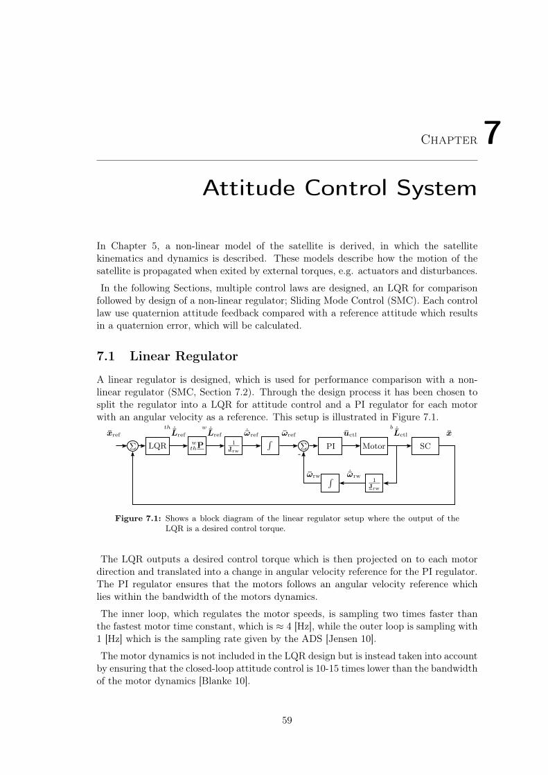
Chapter 7
Attitude Control System
In Chapter 5, a non-linear model of the satellite is derived, in which the satellitekinematics and dynamics is described. These models describe how the motion of thesatellite is propagated when exited by external torques, e.g. actuators and disturbances.
In the following Sections, multiple control laws are designed, an LQR for comparisonfollowed by design of a non-linear regulator; Sliding Mode Control (SMC). Each controllaw use quaternion attitude feedback compared with a reference attitude which resultsin a quaternion error, which will be calculated.
7.1 Linear Regulator
A linear regulator is designed, which is used for performance comparison with a non-linear regulator (SMC, Section 7.2). Through the design process it has been chosen tosplit the regulator into a LQR for attitude control and a PI regulator for each motorwith an angular velocity as a reference. This setup is illustrated in Figure 7.1.
PI Motor SC
1Jrw
∫1
Jrw
∫LQR
-Σ
xref x
Σ
th ˙Lref ˙ωref
wthP
ωref
w ˙Lref
ωrw ˙ωrw
b ˙Lctluctl
Figure 7.1: Shows a block diagram of the linear regulator setup where the output of theLQR is a desired control torque.
The LQR outputs a desired control torque which is then projected on to each motordirection and translated into a change in angular velocity reference for the PI regulator.The PI regulator ensures that the motors follows an angular velocity reference whichlies within the bandwidth of the motors dynamics.
The inner loop, which regulates the motor speeds, is sampling two times faster thanthe fastest motor time constant, which is ≈ 4 [Hz], while the outer loop is sampling with1 [Hz] which is the sampling rate given by the ADS [Jensen 10].
The motor dynamics is not included in the LQR design but is instead taken into accountby ensuring that the closed-loop attitude control is 10-15 times lower than the bandwidthof the motor dynamics [Blanke 10].
59

7. Attitude Control System
7.1.1 Linear System Model
The non-linear system equation ?? is linearised in the point of operation where thesatellite BRF is aligned with the ORF, which means the satellite is pointing Nadir andthe angular velocities is infinitesimal small.
The states x measured at the output of the “SC” block in Figure 7.1 is given as:
x =
[cqscωs
](7.1)
where cqs is the quaternion attitude representation and cωs is the satellite angularvelocity. The states is given in CRF.
The system model is linearised with a first order Taylor approximation, where thegeneral form is
f(x) ≈ f(x) +∂f(x)
∂x
∣∣∣∣x=x
·∆x (7.2)
x = x+∆x (7.3)
where
x is the function variablex is the point of linearisation∆x is small deviation form the linearisation
The angular velocity of the satellite is then approximated to be equal to:
cωs ≈ cbR
0b ˇωo
0
+∆c ˜ωs (7.4)
where ∆c ˜ωs is small perturbations in the angular velocity and b ˇωref is the point of
linearisation, which is the angular velocity of the BRF relative to ECI when alignedwith the ORF.
The attitude cqs is linearised in the orientation of the ORF as shown 7.5.
cqs ≈ cqo ⊗∆ cqs (7.5)
Where cqo is the orbit attitude and linearisation point, and ∆ cqs is the deviation fromthe point of operation. Furthermore it is seen when left multiplying with the conjugatedrotation, the error quaternion appears.
cq∗o ⊗ cqs ≈ cq∗
o ⊗ cqo ⊗∆ cqs
cqe ≈ ∆ cqs(7.6)
From this expression it is seen that the point of linearisation is indeed defined where thequaternion error cqe = [0 0 0 1]>.
60

7.1. Linear Regulator
7.1.2 Linear Kinematics
From equation 7.6 the kinematic equation can be written as small changes in the attitudefor each time interval
∆c ˙qs =
1
2Ω(cωs)∆
cqs (7.7)
The attitude can as stated by equation 5.3 be approximated with the small angleapproximation.
∆ cqs ≈[∆
c ˜qs1
](7.8)
From this it is seen that ∆qs4 ≈ 1 which makes ∆ ˙qs4 ≈ 0. The kinematic equation isthen reduced to the complex part of the quaternion derivative.
The reduced kinematic equation is then linearised in the point of operation.
c ˙qs (cωs,
cqs) ≈c ˙qs
(c ˇωo,c ˇqo
)+
∂c ˙qs (
cωs,cqs)
∂ cqs
∣∣∣∣c ˇωo,
c ˇqo
·∆ c ˜qs (7.9)
+∂
c ˙qs (cωs,
cqs)
∂ cωs
∣∣∣∣c ˇωo,
c ˇqo
·∆ c ˜ωs
where the Jacobian is given as
∂c ˙qs (
cωs,cqs)
∂ cqs
∣∣∣∣c ˇωo,
c ˇqo
=1
2S(c ˇωo
)(7.10)
∂c ˙qs (
cωs,cqs)
∂ cωs
∣∣∣∣c ˇωo,
c ˇqo
=1
2I3×3 (7.11)
where ∆qs4 = 1.
7.1.3 Linearised Dynamic Model
The satellite dynamics is given as:
c ˙ωs = J−1s
[−S (cωs)
cLs − S (cωs)
cLth +
c ˙Lth +c ˙Ld
](7.12)
The disturbance torquec ˙Ld is assumed to have an expected value of zero and is therefore
removed in the linearised equations [Jensen 10]. Furthermore, the Coriolis term fromthe resulting angular moment of the actuators −S (cωs)
cLth ≈ 0 and is neglected in the
linearisation. This is due to the internal cancellation of momentum in the Tetrahedronconfiguration when operating at the biased angular velocities.
Left is the Coriolis term from the satellites angular momentum where the first orderTaylor approximation is used.
− J−1s S (cωs)
cLs ≈ −J−1
s S(c ˇωo
)Js
c ˇωo − J−1s
∂(S(c ˇωo
)Js
c ˇωo
)∂
c ˇωo·∆ c ˜ωs (7.13)
The Jacobian is then found by using the product rule when partially derivingcrossproducts.
Acωs= −J−1
s
∂(S(c ˇωo
)Js
c ˇωo
)∂
c ˇωo= J−1
s
[S(Js
c ˇωo
)− S
(c ˇωo
)Js
](7.14)
61

7. Attitude Control System
7.1.4 State-Space Model
For now the kinematic and dynamic equations has been linearised in a point of operationby a first order Taylor approximations. The derived Jacobians is now used to constructa state-space system of the satellite. Where the states x and inputs u is given as
x =
[cqec ˜ωs
], u =
c ˙Lth (7.15)
Recall from equation 7.6 that cqe ≈ ∆ cqs
˙x =
[12S
(c ˇωo
)12I3×3
03×3 Acωs
]x+
03×3
−J−1s
u (7.16)
7.1.5 Design of LQR
Source: [Sørensen 10]
At this point, a continuous state-space model of the satellite has been constructed inEquation (7.16). In the live implementation, the states would be measured in discretetime intervals, therefore a discrete state-space model is used with a discrete notation.
xk+1 = Φxk + Γuk (7.17)
The aim of the regulator is optimal state feedback in the sense that it finds an inputsignal uk which brings the system to a zero state where x = 0 in an optimal solutionto draw the system states towards the reference point with as little control effort aspossible. This control problem is formulated by assigning a cost to each state and input.This is done by minimizing the deterministic cost function
J (xk, uk) =1
2
∞∑k=0
(x>k Qxk + u>
k Ruk
)(7.18)
Where Q = Q> ≥ 0 and R = R> > 0 are weighting matrices which punishesrespectively the deviation of the state error and the control signal. These are usedas design parameters and found by simulating the system.
The optimal control input to time k can then be found by
uk = −Lkxk (7.19)
where the control gain Lk is given as
Lk =[R+ Γ>Sk+1Γ
]−1Γ>Sk+1Φ (7.20)
andSk = Q+Φ>Sk+1 [Φ− ΓLk] (7.21)
The optimal control gain is found by recursive calculations of Lk and Sk for a giventime horizon N . In this thesis an infinite time horizon LQR, N → ∞, is designed wherethe feedback gains are constant. In this case L0 is found when the condition that therecursive function Sk converge where Sk ≈ Sk+1 which leads to an Algebraic RiccatiEquation.
62
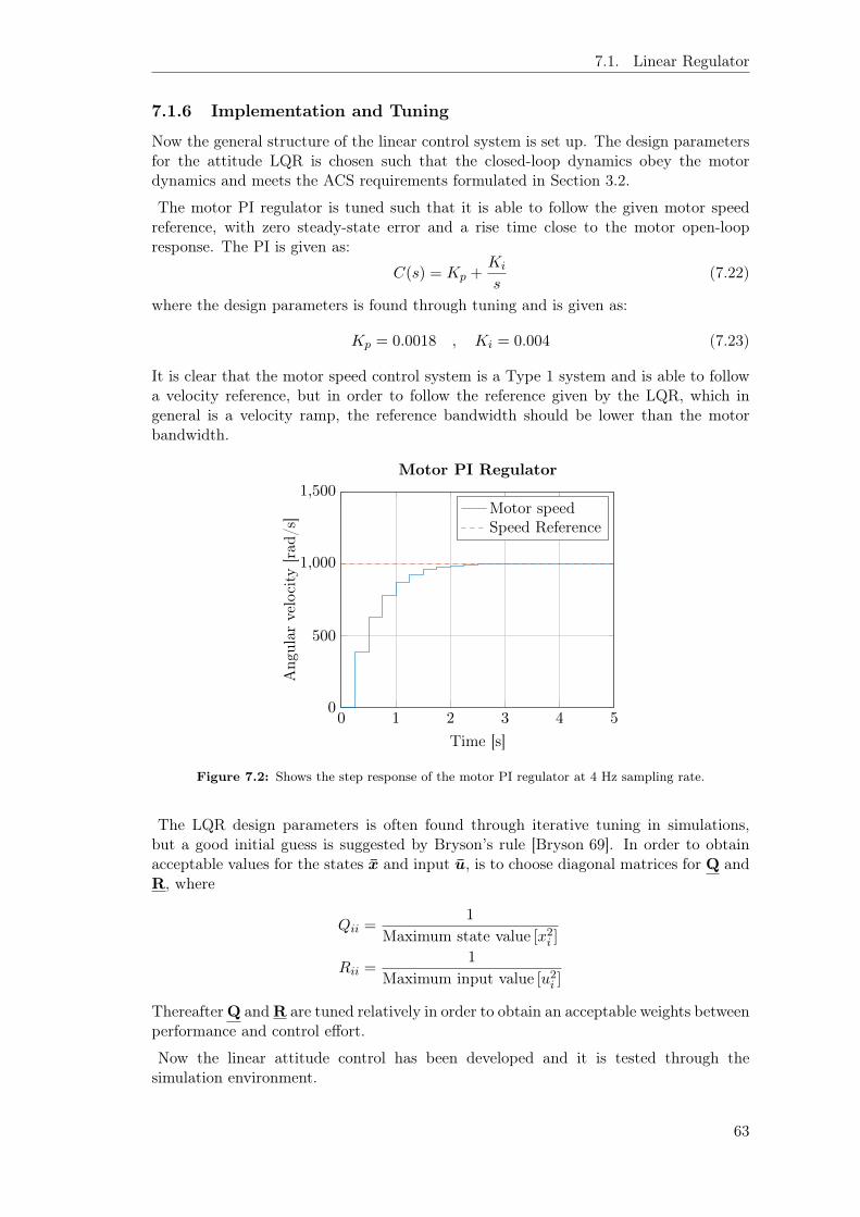
7.1. Linear Regulator
7.1.6 Implementation and Tuning
Now the general structure of the linear control system is set up. The design parametersfor the attitude LQR is chosen such that the closed-loop dynamics obey the motordynamics and meets the ACS requirements formulated in Section 3.2.
The motor PI regulator is tuned such that it is able to follow the given motor speedreference, with zero steady-state error and a rise time close to the motor open-loopresponse. The PI is given as:
C(s) = Kp +Ki
s(7.22)
where the design parameters is found through tuning and is given as:
Kp = 0.0018 , Ki = 0.004 (7.23)
It is clear that the motor speed control system is a Type 1 system and is able to followa velocity reference, but in order to follow the reference given by the LQR, which ingeneral is a velocity ramp, the reference bandwidth should be lower than the motorbandwidth.
0 1 2 3 4 50
500
1,000
1,500
Time [s]
Ang
ular
velo
city
[rad
/s]
Motor PI Regulator
Motor speedSpeed Reference
Figure 7.2: Shows the step response of the motor PI regulator at 4 Hz sampling rate.
The LQR design parameters is often found through iterative tuning in simulations,but a good initial guess is suggested by Bryson’s rule [Bryson 69]. In order to obtainacceptable values for the states x and input u, is to choose diagonal matrices for Q andR, where
Qii =1
Maximum state value [x2i ]
Rii =1
Maximum input value [u2i ]
Thereafter Q and R are tuned relatively in order to obtain an acceptable weights betweenperformance and control effort.
Now the linear attitude control has been developed and it is tested through thesimulation environment.
63

7. Attitude Control System
7.1.7 Results
The linear regulator is tested through two scenarios. First Nadir pointing and thentarget tracking.
Nadir Pointing
The first simulation shows the case where the satellite attitude control is initialised justafter the de-tumbling has been performed. In this situation, the satellite is initialisedwith an absolute 90 deg attitude error and an initial spin of ≈ 0.3 deg/s [Jensen 10] inany axis. The satellite attitude control should then dampen the spin and correct theattitude to point Nadir.
0 10 20 30 40 50 60 70 80 90 100
−50
0
50
Time [s]
Ang
leE
rror
[deg
]
RollPitchYaw
Figure 7.3: Shows the satellite attitude error in Euler angles, where the dashed linesrepresent the maximum error values.
0 10 20 30 40 50 60 70 80 90 100
0
0.5
1
Time [s]
Qua
tern
ion
[-]
q1q2q3q4
Figure 7.4: Shows the satellite attitude bqs relative to the ECI, where the dashed linesrepresent the quaternion attitude reference bqref .
64

7.1. Linear Regulator
0 10 20 30 40 50 60 70 80 90 1000
500
1,000
1,500
Time [s]
Ang
ular
velo
city
[rad
/s] RW1
RW2RW3RW4
Figure 7.5: Shows angular velocities on each motor in the Tetrahedron configuration.
0 10 20 30 40 50 60 70 80 90 1000
1
2
3
Time [s]
Vol
tage
[V]
RW1RW2RW3RW4
Figure 7.6: Shows the motor control signal.
From Figure 7.3 it is seen that the attitude controller manages to slow the initialvelocity down and rotate the satellite to align with the ORF and thereby point Nadir.The attitude is well within the boundaries of the attitude error requirements as it is seenin the given time period.
Target Tracking
In the next scenario the satellite is initialised to point Nadir and an expected point ofinterest is coming into the satellites line of sight. The satellite should then break fromthe ORF to begin pointing at the specific TRF, when in sight. During the pass therewill be an increase in the angular velocity reference from the TRF as the satellite fliesover the interest point, which it should follow.
65
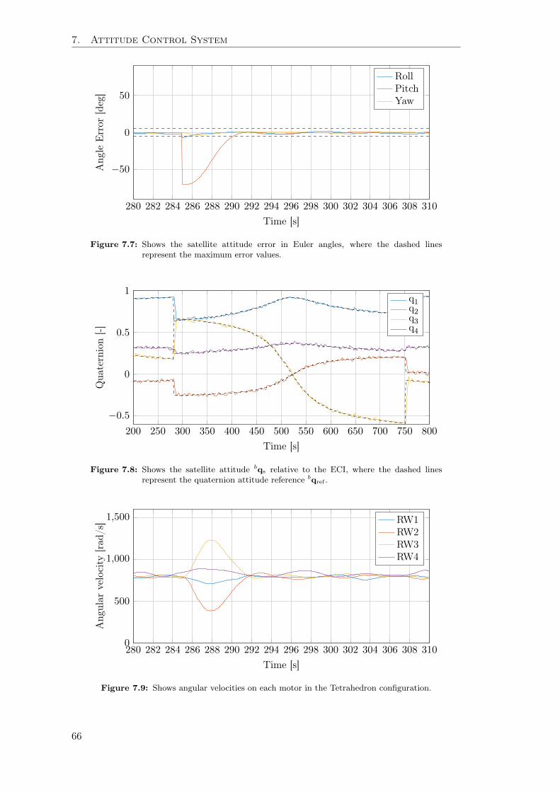
7. Attitude Control System
280 282 284 286 288 290 292 294 296 298 300 302 304 306 308 310
−50
0
50
Time [s]
Ang
leE
rror
[deg
]
RollPitchYaw
Figure 7.7: Shows the satellite attitude error in Euler angles, where the dashed linesrepresent the maximum error values.
200 250 300 350 400 450 500 550 600 650 700 750 800
−0.5
0
0.5
1
Time [s]
Qua
tern
ion
[-]
q1q2q3q4
Figure 7.8: Shows the satellite attitude bqs relative to the ECI, where the dashed linesrepresent the quaternion attitude reference bqref .
280 282 284 286 288 290 292 294 296 298 300 302 304 306 308 3100
500
1,000
1,500
Time [s]
Ang
ular
velo
city
[rad
/s] RW1
RW2RW3RW4
Figure 7.9: Shows angular velocities on each motor in the Tetrahedron configuration.
66
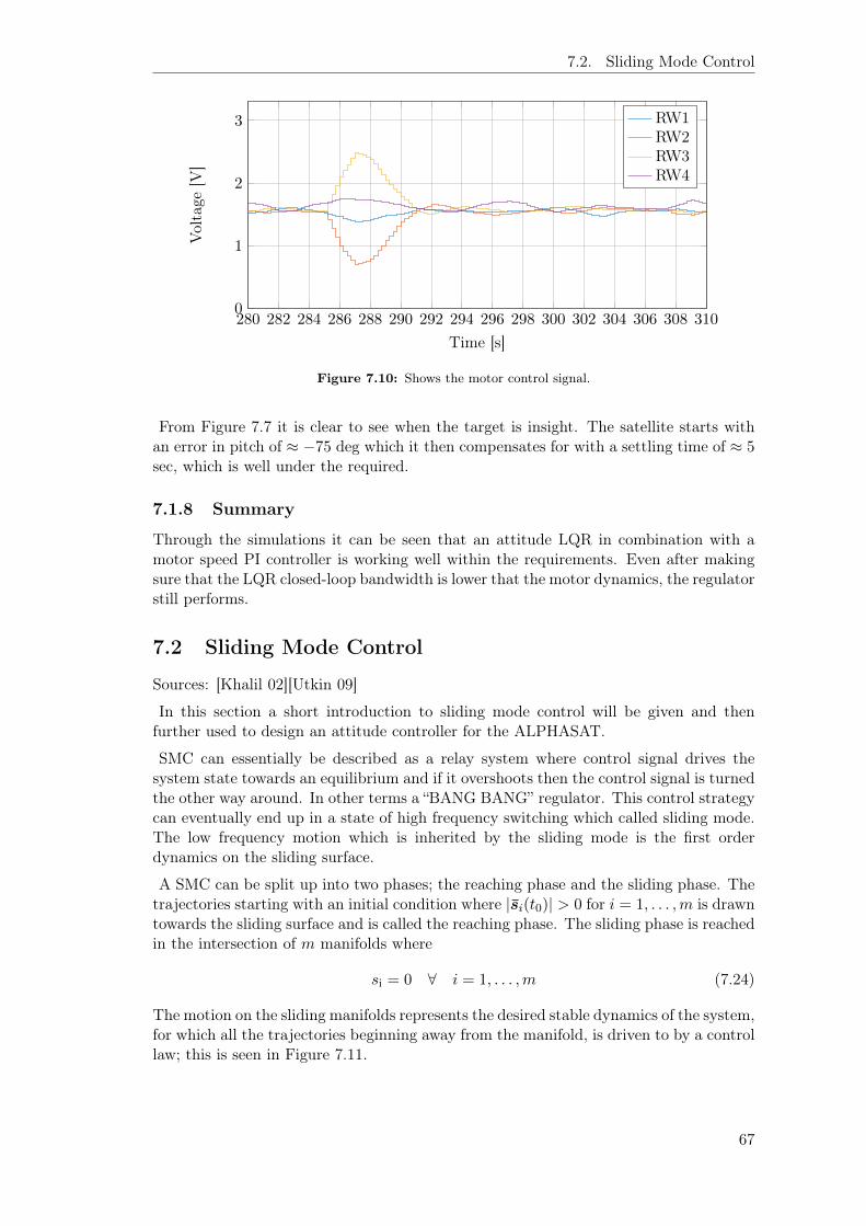
7.2. Sliding Mode Control
280 282 284 286 288 290 292 294 296 298 300 302 304 306 308 3100
1
2
3
Time [s]
Vol
tage
[V]
RW1RW2RW3RW4
Figure 7.10: Shows the motor control signal.
From Figure 7.7 it is clear to see when the target is insight. The satellite starts withan error in pitch of ≈ −75 deg which it then compensates for with a settling time of ≈ 5sec, which is well under the required.
7.1.8 Summary
Through the simulations it can be seen that an attitude LQR in combination with amotor speed PI controller is working well within the requirements. Even after makingsure that the LQR closed-loop bandwidth is lower that the motor dynamics, the regulatorstill performs.
7.2 Sliding Mode Control
Sources: [Khalil 02][Utkin 09]
In this section a short introduction to sliding mode control will be given and thenfurther used to design an attitude controller for the ALPHASAT.
SMC can essentially be described as a relay system where control signal drives thesystem state towards an equilibrium and if it overshoots then the control signal is turnedthe other way around. In other terms a “BANG BANG” regulator. This control strategycan eventually end up in a state of high frequency switching which called sliding mode.The low frequency motion which is inherited by the sliding mode is the first orderdynamics on the sliding surface.
A SMC can be split up into two phases; the reaching phase and the sliding phase. Thetrajectories starting with an initial condition where |si(t0)| > 0 for i = 1, . . . ,m is drawntowards the sliding surface and is called the reaching phase. The sliding phase is reachedin the intersection of m manifolds where
si = 0 ∀ i = 1, . . . ,m (7.24)
The motion on the sliding manifolds represents the desired stable dynamics of the system,for which all the trajectories beginning away from the manifold, is driven to by a controllaw; this is seen in Figure 7.11.
67

7. Attitude Control System
Reaching Phase
Sliding Phase
x
x
si (x, x) = 0
t0
Figure 7.11: Shows how the trajectory is drawn towards the sliding surface, si andeventually the equilibrium point.
The control is given as a discontinuous function of the system states, ui, which isdescribed as a sign function where the control is given as
ui(x, t) = sign(si) =
u+i (x, t) if si (x) > 0
u−i (x, t) if si (x) < 0, i = 1, . . . ,m (7.25)
To reduce the high frequency “chattering” a saturation function can be defined, whichessentially is a continuous approximation of a discontinuous control. This saturationfunction is shown by
ui (x, t) = sat (si) =
sign (si) if ‖si‖ > εsiε if ‖si‖ ≤ ε
(7.26)
where ε defines a saturated area around the sliding surface and dampens the highfrequency switching.
7.2.1 Design of the Sliding Manifold
First a coordinate transformation of the dynamic and kinematic models of the satelliteare performed. This results in an equilibrium point in the origin. Then a sliding manifoldis designed on which the order of the system is reduced. In order drive the system tothe sliding manifold and contain it there for all future time, a control law is designed.
7.2.2 Quaternion Error Calculation
Let bqe denote the relative error between the desired attitude and the current attitude ofthe satellite, given in the body reference frame. This quaternion error is found throughquaternion multiplication as shown:
bqe =bqref ⊗ bq−1
s (7.27)
The relative angular velocity error is denoted by bωe and is given as
bωe =bωref − b
cRcωs (7.28)
With these change of variables the equilibrium point of the system is now moved to theorigin where bqe = [0 0 0 1]> and bqe = [0 0 0 0]>, which is where the angular velocity
68

7.2. Sliding Mode Control
of the satellite bωe = [0 0 0]>. The system model described in section ?? can then berewritten to the given form.
b ˙qebqe4b ˙ωe
=
T(bqe
)bωe
−12bq>e
bωe
b ˙ωref − bcRJ−1
s
[− S(cωs)
cLs − S(cωs)
cLth −
c ˙Lth +c ˙Ld
] (7.29)
where T(q) is a quaternion transformation function which consists of a skew-symmetriccross-product operator from the quaternion derivative with the real values on thediagonal as shown in equation 7.30.
T(q) = −1
2
[S(q)− q4I 3×3
](7.30)
The quaternion dynamics b ¨qe consists of the satellite error dynamics which is shown inequation 7.31.
b ˙ωe =b ˙ωref − b
cRJ−1s
[− S(cωs)
cLs(
cωs, t)
+c ˙Lth(
bωs, ωm, u, t) +c ˙Ld(t)
] (7.31)
Where the external moment componentc ˙Lth(
bωs, ωm, u, t) originates from the resultingmoments generated by the Tetrahedron reaction wheel configuration and is given as.
c ˙Lth
th ˙Lc
th ˙Lcor
=
− c
thR
(th ˙Lcor(
bωs, ωm, t) +th ˙Lc(ωm, u, t)
)thwP (−Λmωm + Γmum)
4∑i=1
−withPS (wiωs +
wiωmi)Jwi(wiωs +
wiωmi)
(7.32)
Where um is the control input vector where the entries represents the voltage across
each motor, controlling the motor torqueth ˙Lc.
The control objective is then to drive the system states from an initial state[bq>
e (0),bq>
e (0)]> to the desired attitude and angular velocity
[bq>
ref(t),bq>
ref(t)]> within
a finite time t.
7.2.3 Sliding Manifold
The sliding manifold is designed as shown in equation 7.33.
s =b ˙qe +K bqe = 0 (7.33)
where:b ˙qe is the quaternion error kinematicsbqe is the quaternion errorK is a real, positive definite, diagonal matrix
All motion on the sliding surface is then governed by the first order dynamics writtenas
b ˙qe = −K bqe (7.34)
Further it is shown that the motion on the manifold in equation 7.33 is proven to bestable by the Lyapunov stability criteria.
69

7. Attitude Control System
Stability on the sliding surface is investigated by a chosen quadratic Lyapunov function:
Vs
(bqe
)=
1
2bq>e
bqe > 0 in D − 0 ,bqe ∈ D :
∥∥∥bqe∥∥∥ ≤ 1
(7.35)
where D ⊂ R3, Vs
(bqe
)is positive definite and Vs(0) = 0 is the origin of the Lyapunov
function. The derivative of the Lyapunov function is then
Vs
(bqe
)=
1
2b ˙q>e
bqe +1
2bq>e
b ˙qe
= bq>eb ˙qe ≤ 0
(7.36)
The origin is proven to be stable if the inequality V ≤ 0 holds for the entire domain D.By inserting the dynamics of the sliding surface equation 7.34 into equation 7.36 yields
Vs
(bqe
)= − bq>e K
bqe < 0 in D − 0 (7.37)
which is negative definite which means that all motion on the sliding surface isasymptotically stable.
7.2.4 The Reaching Phase
For now a sliding surface is designed, upon which, all motion is bounded by a reducedorder dynamics. Next step is to design a control law which drives all the trajectoriestowards the sliding manifold.
In order to investigate if all the trajectories starting off the sliding surface where|s(0)| > 0 goes towards s(t) = 0 when t → ∞, a Lyapunov function is constructed.
The Lyapunov function represents a quadratic function of the sliding surface which ispositive semi-definite.
V (s) =1
2s>s > 0 in D − 0 , V (0) = 0; (7.38)
which indeed is positive definite and only zero at the origin. In order to prove stabilitythe derivative of the Lyapunov function is investigated.
V (s) =1
2s> ˙s+
1
2˙s>s = s> ˙s (7.39)
where ˙s is given as˙s =
b ¨qe +Kb ˙qe (7.40)
by inserting the derivative of the sliding surface ˙s into equation 7.39.
V (s) = s> ˙s = s>[b ¨qe +K
b ˙qe
]= s>
[T(bqe) ˙ωe −
1
4bqe ‖ωe‖22 +K
b ˙qe
] (7.41)
By inserting the error dynamics ˙ωe from equation 7.31 into 7.41 the control um appears.
V (s) = s>[T(bqe) ˙ωref −T(bqe)
bcRJ−1
s
(− S(cωs)
cLs − c
thRth ˙Lcor
+ cthR
thwPΛmωm − c
thRthwPΓmum +
c ˙Ld(t))
− 1
4bqe
∥∥∥bωe
∥∥∥22+K
b ˙qe
] (7.42)
70
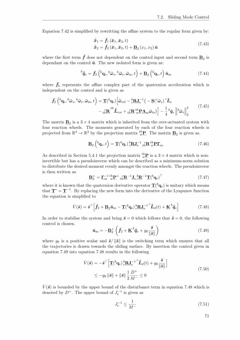
7.2. Sliding Mode Control
Equation 7.42 is simplified by rewritting the affine system to the regular form given by:
˙x1 = f1 (x1, x2, t)
˙x2 = f2 (x1, x2, t) +B2 (x1, x2) u(7.43)
where the first term f dose not dependent on the control input and second term B2 isdependant on the control u. The new isolated form is given as:
b ¨qe = f2
(bqe,
bωs,bωe, ωm, t
)+B2
(bqe, t
)um (7.44)
where fb represents the affine complex part of the quaternion acceleration which isindependent on the control and is given as
f2
(bqe,
bωs,bωe, ωm, t
)= T(bqe)
[˙ωref − b
cRJ−1s
(− S(cωs)
cLs
− cthR
th ˙Lcor +c
thRthwPΛmωm
)]− 1
4bqe
∥∥∥bωe
∥∥∥22
(7.45)
The matrix B2 is a 3× 4 matrix which is inherited from the over-actuated system withfour reaction wheels. The moments generated by each of the four reaction wheels isprojected from R4 → R3 by the projection matrix th
wP. The matrix B2 is given as.
B2
(bqe, t
)= T(bqe)
bcRJ−1
sc
thRthwPΓm (7.46)
As described in Section 5.4.1 the projection matrix thwP is a 3× 4 matrix which is non-
invertible but has a pseudoinverse which can be described as a minimum-norm solutionto distribute the desired moment evenly amongst the reaction wheels. The pseudoinverseis then written as
B+2 = Γ−1
mthwP
+ cthR
−1JsbcR
−1T(bqe)> (7.47)
where it is known that the quaternion derivative operator T(bqe) is unitary which meansthat T∗ = T−1. By replacing the new form into the derivative of the Lyapunov functionthe equation is simplified to
V (s) = s>[f2 +B2um −T(bqe)
bcRJ−1
s
c ˙Ld(t) +Kb ˙qe
](7.48)
In order to stabilise the system and bring s = 0 which follows that ˙s = 0, the followingcontrol is chosen.
um = −B+2
(f2 +K
b ˙qe + g0s
‖s‖
)(7.49)
where g0 is a positive scalar and s/ ‖s‖ is the switching term which ensures that allthe trajectories is drawn towards the sliding surface. By insertion the control given inequation 7.49 into equation 7.48 results in the following
V (s) = −s>[T(bqe)
bcRJ−1
s
c ˙Ld(t) + g0s
‖s‖
]≤ −g0 ‖s‖+ ‖s‖ 1
2
D+
M− ≤ 0
(7.50)
V (s) is bounded by the upper bound of the disturbance term in equation 7.48 which isdenoted by D+. The upper bound of J−1
s is given as
J−1s ≤ 1
M− (7.51)
71

7. Attitude Control System
where M− > 0 and represents the smallest MoI of the satellite. The knowledge of theworst case disturbance, a lower bound for the switching gain g0 is derived.
g0 ≥1
2
D+
M− + σ0 , σ0 > 0 (7.52)
if g0 is inserted into 7.50 the following inequality appearers.
V (s) ≤ −σ0 ‖s‖ (7.53)
where this inequality ensures that all trajectories starting off the sliding manifold wheres = 0 will reach it within a finite time depending on the size of σ0.
In this particular case, the size of the switching gain g0 is only dependant on themagnitude of the disturbance and σ0. This is only valid if the dynamic model is withoutuncertainties. In models with large uncertainties the control would again consist ofa continuous part dependant on the nominal model of the satellite and a switchingpart, which magnitude would depend on the upper-bounds of the uncertainty from thenominal model. These uncertainties could result in large switching gains which wouldintroduce “chattering” when crossing the sliding surface as illustrated in Figure 7.11.The chattering is reduced by applying a saturation function as described in equation7.26.
Now that the sliding mode attitude controller is designed it should be verified throughthe simulation environment.
7.2.5 Results
The SMC is in general verified with the same simulation configuration as the linearregulator, in order to perform a genuine performance comparison.
Nadir Pointing
The satellite is first initialised in an arbitrary orientation with an initial spin, same asthe linear attitude controller simulation. The controller should then bring align thesatellite attitude with the ORF in order to point Nadir.
0 10 20 30 40 50 60 70 80 90 100
−50
0
50
Time [s]
Ang
leE
rror
[deg
]
RollPitchYaw
Figure 7.12: Shows the satellite attitude error in Euler angels, where the dashed linesrepresent the maximum and minimum angle error.
72
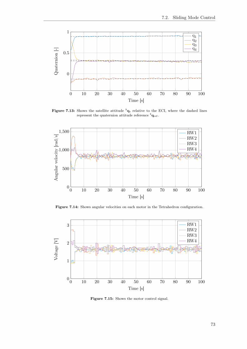
7.2. Sliding Mode Control
0 10 20 30 40 50 60 70 80 90 100
0
0.5
1
Time [s]
Qua
tern
ion
[-]
q1q2q3q4
Figure 7.13: Shows the satellite attitude bqs relative to the ECI, where the dashed linesrepresent the quaternion attitude reference bqref .
0 10 20 30 40 50 60 70 80 90 1000
500
1,000
1,500
Time [s]
Ang
ular
velo
city
[rad
/s] RW1
RW2RW3RW4
Figure 7.14: Shows angular velocities on each motor in the Tetrahedron configuration.
0 10 20 30 40 50 60 70 80 90 1000
1
2
3
Time [s]
Vol
tage
[V]
RW1RW2RW3RW4
Figure 7.15: Shows the motor control signal.
73

7. Attitude Control System
From Figure 7.12 it is seen that the angular error in Roll, Pitch and Yaw is compensatedfor within ≈ 4 sec. which is well within the requirements.
Target Tracking
280 282 284 286 288 290 292 294 296 298 300 302 304 306 308 310
−50
0
50
Time [s]
Ang
leE
rror
[deg
]
RollPitchYaw
Figure 7.16: Shows the satellite attitude error in Euler angels.
200 250 300 350 400 450 500 550 600 650 700 750 800
−0.5
0
0.5
1
Time [s]
Qua
tern
ion
[-]
q1q2q3q4
Figure 7.17: Shows the satellite attitude bqs relative to the ECI, where the dashed linesrepresent the quaternion attitude reference bqref .
74

7.2. Sliding Mode Control
280 282 284 286 288 290 292 294 296 298 300 302 304 306 308 3100
500
1,000
1,500
Time [s]
Ang
ular
velo
city
[rad
/s] RW1
RW2RW3RW4
Figure 7.18: Shows angular velocities on each motor in the Tetrahedron configuration.
280 282 284 286 288 290 292 294 296 298 300 302 304 306 308 3100
1
2
3
Time [s]
Vol
tage
[V]
RW1RW2RW3RW4
Figure 7.19: Shows the motor control signal.
7.2.6 Summary
The sliding mode control algorithm is a quaternion based sliding mode, whichs takesthe coriolis torques from the reaction wheels into account. Through the simulations itcan be seen that the sliding mode attitude control algorithm performs well within therequirements.
75


Chapter 8
Attitude Control Testbed
Attitude Determination and Control Systems for CubeSat satellites are inherentlydifficult to test and validate. This is because of both the relatively small actuationtorques available and the environment present at the Earth’s surface level, comparedto the environment at LEO altitudes. When designing attitude control algorithms fora spacecraft as small as a CubeSat, the physical size of the spacecraft impose innateconstraints on the dimensioning of the actuators and thereby inherently also on theactuator torques available. The small actuator torques available, hence presents achallenge when the control algorithms is to be validated in a live implementation.
To accommodate for these challenges, a testbed is designed and built in order to permittesting capabilities of the attitude control algorithms designed for ALPHASAT and otherfuture projects at AAU.
A testbed can be a valuable tool, both in the design processes of the next student builtsatellites at AAU but also for use in education and semester projects.
AAU Student Space has, in the time of writing, launched five student built CubeSatsatellites. The satellites, AAUSAT3 and 4 both used magnetic actuation for attitudecontrol. During LEOPs of both satellites, the detumbling algorithm where initiatedwhich eventually caused the satellites to accelerate instead of decelerate. A wrong signin the detumbling algorithm caused this unfortunate error.
The test phase of both satellites might have benefited by having an attitude controltestbed. This could have provided the ability to perform, not only, active pointingtesting, but also the ability to perform basic sanity checks of the algorithms. These aretwo examples of cases without severe consequences, as this sign where simply changedwhen the fault where registered. However if this sign was not easily changed this couldhave led to the loss of the satellites.
Another example, is the rotations performed within an attitude control algorithm. Theability to perform sanity checks of these can be beneficial as an addition to simulationsduring the design and test phase, of a satellite mission.
The attitude control testbed designed throughout, the following chapter, aims toprovide a method of testing the general properties and ability to perform sanity checkson control algorithms. In addition to this, an attitude control testbed provides aneducational tool for implementing three-dimensional control algorithms.
The testbed does however not provide the ability to test and validate the exactcontrollers designed for a spacecraft, this would require a mechanical design allowingan actual satellite to be inserted into the testbed. A typical satellite consists of rather
77
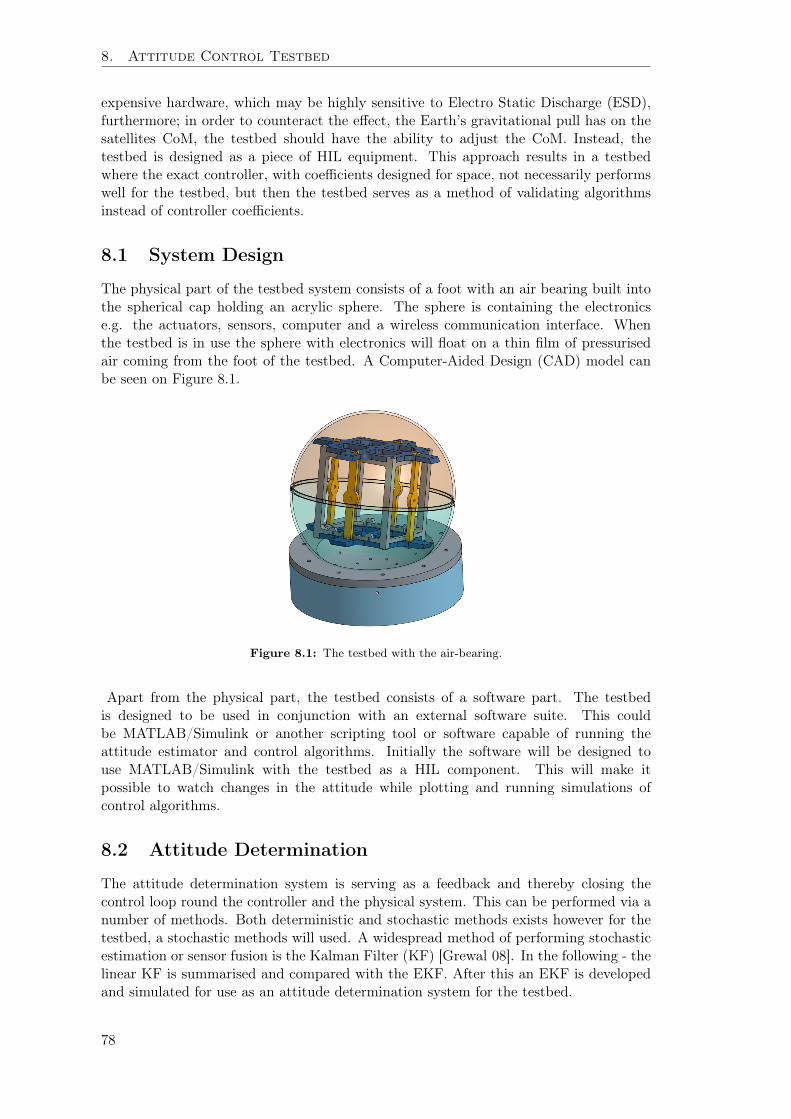
8. Attitude Control Testbed
expensive hardware, which may be highly sensitive to Electro Static Discharge (ESD),furthermore; in order to counteract the effect, the Earth’s gravitational pull has on thesatellites CoM, the testbed should have the ability to adjust the CoM. Instead, thetestbed is designed as a piece of HIL equipment. This approach results in a testbedwhere the exact controller, with coefficients designed for space, not necessarily performswell for the testbed, but then the testbed serves as a method of validating algorithmsinstead of controller coefficients.
8.1 System Design
The physical part of the testbed system consists of a foot with an air bearing built intothe spherical cap holding an acrylic sphere. The sphere is containing the electronicse.g. the actuators, sensors, computer and a wireless communication interface. Whenthe testbed is in use the sphere with electronics will float on a thin film of pressurisedair coming from the foot of the testbed. A Computer-Aided Design (CAD) model canbe seen on Figure 8.1.
Figure 8.1: The testbed with the air-bearing.
Apart from the physical part, the testbed consists of a software part. The testbedis designed to be used in conjunction with an external software suite. This couldbe MATLAB/Simulink or another scripting tool or software capable of running theattitude estimator and control algorithms. Initially the software will be designed touse MATLAB/Simulink with the testbed as a HIL component. This will make itpossible to watch changes in the attitude while plotting and running simulations ofcontrol algorithms.
8.2 Attitude Determination
The attitude determination system is serving as a feedback and thereby closing thecontrol loop round the controller and the physical system. This can be performed via anumber of methods. Both deterministic and stochastic methods exists however for thetestbed, a stochastic methods will used. A widespread method of performing stochasticestimation or sensor fusion is the Kalman Filter (KF) [Grewal 08]. In the following - thelinear KF is summarised and compared with the EKF. After this an EKF is developedand simulated for use as an attitude determination system for the testbed.
78
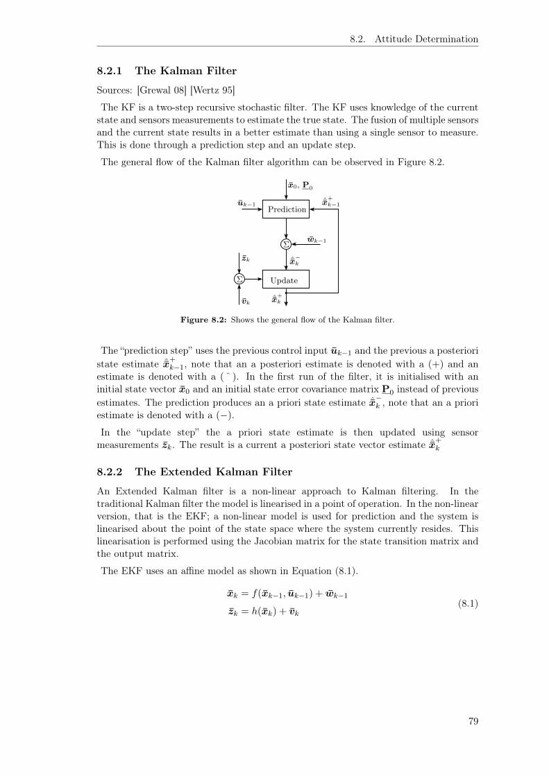
8.2. Attitude Determination
8.2.1 The Kalman Filter
Sources: [Grewal 08] [Wertz 95]
The KF is a two-step recursive stochastic filter. The KF uses knowledge of the currentstate and sensors measurements to estimate the true state. The fusion of multiple sensorsand the current state results in a better estimate than using a single sensor to measure.This is done through a prediction step and an update step.
The general flow of the Kalman filter algorithm can be observed in Figure 8.2.
Σ
Prediction
Update
wk−1
ˆx−k
zk
ˆx+k
Σ
vk
x0, P0
uk−1ˆx+k−1
Figure 8.2: Shows the general flow of the Kalman filter.
The “prediction step” uses the previous control input uk−1 and the previous a posterioristate estimate ˆx
+k−1, note that an a posteriori estimate is denoted with a (+) and an
estimate is denoted with a ( ˆ ). In the first run of the filter, it is initialised with aninitial state vector x0 and an initial state error covariance matrix P0 instead of previousestimates. The prediction produces an a priori state estimate ˆx
−k , note that an a priori
estimate is denoted with a (−).
In the “update step” the a priori state estimate is then updated using sensormeasurements zk. The result is a current a posteriori state vector estimate ˆx
+k
8.2.2 The Extended Kalman Filter
An Extended Kalman filter is a non-linear approach to Kalman filtering. In thetraditional Kalman filter the model is linearised in a point of operation. In the non-linearversion, that is the EKF; a non-linear model is used for prediction and the system islinearised about the point of the state space where the system currently resides. Thislinearisation is performed using the Jacobian matrix for the state transition matrix andthe output matrix.
The EKF uses an affine model as shown in Equation (8.1).
xk = f(xk−1, uk−1) + wk−1
zk = h(xk) + vk(8.1)
79

8. Attitude Control Testbed
Where:
x is the system state vector [·]u is the control input [·]w is the process noise [·]z is the measurement vector [·]v is the measurement noise [·]
In the prediction step this model is used to propagate the previous a posteriori stateestimate ˆx
+k−1 and the previous actuator input uk−1, resulting in an a priori state
estimate ˆx−k .
ˆx−k = f( ˆx
+k−1, uk−1) + wk−1 (8.2)
Where:
ˆx−k is the a priori state estimate [·]
ˆx+k−1 is the previous a posteriori state estimate [·]
The process noise wk−1 is assumed white Gaussian noise with mean 0 and covariancematrix Q.
A state transition matrix matrix Φ k is then calculated by the Jacobian matrix. TheΦ k matrix and the process noise covariance matrix Q is used to propagate the previousa posteriori state vector error covariance matrix.
Φ k =∂f(x, uk−1)
∂x
∣∣∣∣x=ˆx
−k
P−k = Φ kP
+k−1Φ
>k +Q
(8.3)
Where:
P−k is the a priori state error covariance matrix [·]
P+k−1 is the previous a posteriori state error covariance matrix [·]
In the update step; the a priori state estimate is updated via a sensor measurement. Thea priori state vector estimate is mapped into an a priori measurement vector estimateˆz−k using a sensor model.
ˆz−k = h( ˆx
−k ) + vk (8.4)
Where:
ˆz−k is the a priori measurement vector estimate [·]
vk is the measurement noise [·]
The measurement noise is assumed white Gaussian noise with mean 0 and covariancematrix R.
80

8.2. Attitude Determination
The sensor model is linearised about the a priori state vector estimate using a Jacobianand a Kalman gain matrix is calculated using the a priori state error covariance matrix,the measurement matrix and the measurement noise covariance matrix.
Hk =∂h(x)
∂x
∣∣∣∣x=ˆx
−k
Kk = P−k H
>k
(HkP
−k H
>k +R
)−1(8.5)
A sensor measurement is performed and the Kalman gain is used to update the a prioristate vector estimate with the measurement prediction error resulting in an a posterioristate vector estimate
ˆx+k = ˆx
−k +Kk
(zk − ˆz
−k
)(8.6)
Where:
zk is the sensor measurements [·]
The last step is to update the a priori state vector covariance matrix into a a posterioristate vector covariance matrix. This is done by utilising the Kalman gain matrix andthe measurement matrix.
P+k = (I−KkHk)P
−k (8.7)
A comparison between the Kalman filter and the Extended Kalman filter algorithmsare shown below. The main difference between the traditional Kalman filter and theEKF is that an extended Kalman filter uses a non-linear prediction model.
Prediction:
KF
ˆx−k = Φ ˆx
+k−1 + Γuk−1 + wk−1
ˆz−k = H ˆx
−k + vk
P−k = ΦP+
k−1Φ> +Q
k−1
EKF
ˆx−k = f( ˆx
+k−1, uk−1) + wk−1
ˆz−k = h( ˆx
−k ) + vk
Φ k =∂f(x, uk−1)
∂x
∣∣∣∣x=ˆx
−k
Hk =∂h(x)
∂x
∣∣∣∣x=ˆx
−k
P−k = Φ kP
+k−1Φ
>k +Q
k−1
(8.8)
Update:
Kk = P−k H
>(HP−
k H> +Rk
)−1Kk = P−
k H>k
(HkP
−k H
>k +Rk
)−1
ˆx+k = ˆx
−k +Kk
(zk − ˆz
−k
)P+
k = (I−KkHk)P−k
The method of using non-linear equations where possible and then linearise the systemat the current state where necessary, does however have a constraint. The constraint isthat it is only possible for sufficiently smooth systems [Grewal 08].
81

8. Attitude Control Testbed
If a system with some irregular dynamics and kinematics, is in a point in its state spacewhere the rate of change in the function is to great compared to the rate that the EKFis running; then the estimate cannot be trusted, because the system can differ to muchfrom its linearisation point. Other methods of estimation must then be considered.
This is however not the case for a satellite and hence not the attitude control testbedeither.
8.2.3 Quaternions and the Extended Kalman Filter
Sources: [Markley 14] [Bak 99] [Markley 03] [Humphreys 02] [Stuelpnagel 64]
A parameter set of four, is the smallest set for which an attitude in a three-dimensionalspace can be represented singularity free [Stuelpnagel 64]. The quaternion is suchparameter set; the only constraint on a quaternion as an attitude representation is a unitnorm constraint. A quaternion is not closed under addition and scalar multiplication,which implies that the quaternion does not span a vector space. The quaternion is asphere in a four-dimensional space. When observing the update equations in Equation(8.9) it becomes apparent that a consequence of not spanning a vector space is that theresulting quaternion can not, with certainty, be a quaternion of unit length, and hencenot the an orthogonality preserving rotation.
Furthermore according to [Bak 99] and [Markley 14]; using a four-dimensional attituderepresentation for something which is inherently three-dimensional, can lead to a singularstate error covariance matrix.
One way to address these challenges is to modify the Kalman filter, such that thequaternion part is updated multiplicatively and thereby adhering to the quaternionalgebra. This results in a Multiplicative Extended Kalman Filter (MEKF). The idea ofthe MEKF is to use a global attitude representation and perturb it with a local “error”representation. This means using an error state vector inside the MEKF. Where thequaternion part of the state vector contains only the vector part of the quaternion;thereby making the covariance propagation possible without singularity problems.
The prediction step is:
ˆx−k = f( ˆx
+k−1, uk−1) + wk−1
ˆz−k = h( ˆx
−k ) + vk
(8.9)
Next step is to calculate the δ ˆx+k which is the vector containing the perturbations for
the global state.δ ˆx
+k = Kk
[zk − ˆz
−k
](8.10)
Where:
δ ˆx+k =
[δ ˆq
+k
δ ˆξ+
k
](8.11)
Where ˆξ−k collects all the states which can be updated the traditional linear way.
Note that the quaternion part ( ˆq−k ) only consists of the imaginary vector part of thequaternion.
82

8.2. Attitude Determination
The quaternion part of δ ˆx+k consists of only the vector part of the quaternion. In order
to enforce the quaternion norm, and thereby ensuring orthogonality, the real part of theδ ˆq
+k is calculated as:
δq+4,k =
√1−
∥∥∥δ ˆq+k ∥∥∥22
(8.12)
The δ ˆq+k is augmented with this and the attitude quaternion updated:
q+k =
[δ ˆq
+k
δq+4,k
]⊗ q−
k (8.13)
The ξ part of the state vector is updated, as with traditional EKFs.
ˆξ+
k = ˆξ−k + δ ˆξ
+
k (8.14)
With this method the covariance singularity problem is addressed and the quaternionnorm is enforced, making this algorithm a good choice for attitude determination.
A summary of the complete algorithm is shown in equations (8.15) and (8.16).
Prediction Step:
ˆx−k = f( ˆx
+k−1, uk−1) + wk−1
ˆz−k = h( ˆx
−k ) + vk
Φ k =∂f(x, uk−1)
∂x
∣∣∣∣x=ˆx
−k
Hk =∂h(x)
∂x
∣∣∣∣x=ˆx
−k
P−k = Φ kP
+k−1Φ
>k +Q
k−1
(8.15)
Update Step:
Kk = P−k H
>k
(HkP
−k H
>k +Rk
)−1
δ ˆx+k = Kk
[zk − ˆz
−k
]
q+k =
δ ˆq+k√
1−∥∥∥δ ˆq+k ∥∥∥2
2
⊗ q−k
ˆξ+
k = ˆξ+
k−1 + δ ˆξ−k
ˆx+k =
[q+k
ˆξ+
k
]P+
k = (I−KkHk)P−k
(8.16)
This concludes the description of this slightly modified EKF, the MEKF. The MEKFis a Kalman filter which takes the quaternion in the state vector into account in
83

8. Attitude Control Testbed
the update step. Taking the quaternion of the state vector into account has theadvantage of adhering to the quaternion norm constraint in the update step, therebyminimising the numerical rounding errors of performing a brute-force normalisation afteran additive update step; furthermore is has the advantage of avoiding the risk of thestate error covariance matrix becoming ill-conditioned or singular described by [Bak 99]and [Markley 14].
8.2.4 Implementation and Tuning
The EKF described in the previous section is implemented in Matlab. This is doneto facilitate the HIL approach of the testbed and have both the control and attitudedetermination algorithms running in Matlab/Simulink.
The states that is to be estimated in the EKF is:
x =
bqs
bωs
ωrw
(8.17)
The attitude quaternion bqs describes the testbed hardware’s attitude relative to theGRF. For a spacecraft in orbit this would be the satellites attitude relative to the ECIinstead. Likewise bωs is the angular velocity of the testbed hardware relative to GRF.The ωrw is the angular velocities of the four reaction wheels.
The models used for estimating these 11 states are developed in Chapter 5 and issummarised in equation (8.18).
cqsc ˙ωs
˙ωrw
=
12Ω(ω)q
J−1s
[−S (cωs)
cLs − S (cωs)
cLth +
c ˙Lth
]J−1rw
[thwP (−Λmωm + Γmum)
] (8.18)
These model are used to propagate the previous a posteriori state estimation to an apriori state estimation. This is done using a forward Euler numerical integration method.
The testbed hardware is equipped with sensors for performing attitude determination.These sensors are: accelerometer, gyroscope and magnetometer, furthermore thereaction wheels is equipped with encoders which enables measurements of the angularvelocities of these. For designing output equations for the MEKF, and for simulationpurposes, the sensor measurements are modelled and presented in the following.
The accelerometer measurements is modelled as a gravity vector in GRF rotated bythe attitude quaternion.
ba = K a
[bgq
∗ gg bgq+ babd
]+ va (8.19)
Where:
K a is a scale factor matrix [·]bgq is the rotation quaternion from GRF to BRF [·]gg is the gravity
[m/s2
]va is the accelerometer noise [·]babd is the linear acceleration of the body
[m/s2
]84

8.2. Attitude Determination
The Gyroscope measurements is modelled as the estimated angular velocity of the body,taken from the state vector, added with gyroscope noise.
bω = K gbωs + vg (8.20)
Where:
bω is the angular velocity measured [rad/s]
K g is a scale factor matrix [·]vg is the gyroscope noise [·]
The magnetometer measurements is modelled similar to the accelerometer. A magneticfield vector pointing north in GRF is rotated by the attitude quaternion.
bh = Km
[bgq
∗ gh b
gq]+ vm (8.21)
Where:
gh is the magnetic field vector pointing north in GRF [·]
Km is a scale factor matrix [·]bgq is the rotation quaternion from GRF to BRF [·]vm is the magnetometer noise [·]
The last of the sensors is the reaction wheel encoders. The reaction wheels angularvelocity is in the state vector of the MEKF, hence the sensor model is:
ωrw = I4×4ωrw + vrw (8.22)
Where:
ωrw is the angular velocities of the reaction wheels [rad/s]
vrw is the encoder noise [rad/s]
The scale factor matrices K a, K g and Km are positive definite matrices which is usedto scale the modelled vector into something comparable to sensor readings. The sensornoises va, vg, vm and vrw is assumed uncorrelated white Gaussian noise with mean zeroand respectively covariance matrices R a, R g, Rm and R rw.
Initial covariance matrices R a, R g, Rm and R rw is found from a sample of sensordata logged from the actual sensors on the built testbed.
The covariance matrices Q, R and P0 is however considered tuning matrices forthe MEKF. This means that the covariance matrix found from sensor analysis isonly considered an initial guess. The MEKF is tuned through an iterative process,first through simulations and since, on the actual testbed to obtain the best possibleperformance for the attitude determination.
The state error covariance matrix to time k = 0, P0, is defined to:
P0 = I10×10 (8.23)
This relative large covariance is set because the filter has no knowledge of the initialstate vector.
85

8. Attitude Control Testbed
The process noise error covariance matrix Q and the measurement noise covariancematrix are defined to:
Q = diag(11×6 · 10−4 11×4 · 10−3
)
R = diag(11×3 · 10−1 11×3 · 3.4 · 10−6 11×3 · 2.23 · 10−3 11×4 · 10−1
)Where diag() is a diagonal matrix with the arguments on its main diagonal.
The Jacobian Matrices
Two Jacobian matrices are used in the MEKF. The first one is the Φk matrix calculatedfrom the system equations. The Φk matrix is calculated as:
Φk = I10×10 +
∂ cqs
∂ cqs
∂ cqs
∂ cωs03×4
03×3∂ cωs
∂ cωs
∂ cωs
∂ωrw
04×3 04×3∂ωrw∂ωrw
· Ts (8.24)
Where Ts is the sample time of the MEKF.
The Hk matrix is calculated as:
Hk =
∂ ba∂ cqs
03×3 03×4
03×3 I3×3 03×4
∂bh
∂ cqs03×3 03×4
04×3 04×3 I4×4
(8.25)
8.3 Simulation
The MEKF presented in the previous Section, is simulated in order to validate itsperformance. For this a simulation environment is constructed in Simulink. TheSimulation environment includes the spacecraft system model and sensor models. Theoutput of the deterministic system models is fed to the sensor models which then outputsa modelled sensor signal used as measurements for the MEKF.
The simulation of the satellite model is initialised with an initial spin of 0.3 deg/sand an attitude of bs,init = [0 0 0.0872 0.9962]> which corresponds to the angularvelocity a CubeSat would have, after it has been detumbled and a quaternion rotationof 10 deg.
The initial states of the MEKF is defined as:
x0 =[qs,init ωs,init ωrw,init
]> (8.26)
where
qs,init =[0 0 0 1
]ωs,init =
[0 0.0052 0
]ωrw,init =
[800 800 800 800
] (8.27)
which will give an initial estimation error of 10 deg. The simulation environment isshown in Figure 8.3.
86

8.3. Simulation
InitialangularvelocityW_i(b)
Initialattitudeq(b)
Controllerframeq(b->c)
SatelliteInertiaI(c)
N_mt(b)
DisturbanceN_dist(b)
Attitudeq_b
AngularvelocityW(b)
SpacecraftDynamics(Alphasat)
q_I_s
mag_I
mag_bias
mag_s_meas
testand_magnetometer
q_I_s
g_I
acc_bias
acc_body
acc_s_meas
teststand_accelerometer
w_s
gyro_bias
gyro_s_meas
teststand_gyro
[010]'
MagVector
[001]'
GravityVector
[000]'
body_acc[0.67140.70440.7268]*1e-3
Constant4
[0001]
Constant5
[000]'
Constant6
[000.08720.9962]
Constant7
[010]'*deg2rad(0.3)
Constant8 [000]'
g_bias
[000]'
gyro_bias
[000]'
Mag_bias
acc_meas
gyro_meas
mag_meas
rw_omega_in
u
q_s_g
omega_s
rw_omega
TeststandEKF
[1111]'*3.3/2
Controlsignal
q1
q2q_diff
Rotationfromq1toq2
[4x1]
RWvelocity
R2D
RadianstoDegrees
InterpretedMATLABFcn
quat2euler
q_s
omega_s
rw_omega
est_error
SaveEKFData
[q_s_g]
[omega_s]
[rw_omega]
[q_s_g]
[omega_s]
[rw_omega]
[q_s_g]
[omega_s]
[rw_omega]
[est_error]
[est_error]
[est_error]
Figure 8.3: Shows the EKF simulation environment
The initial spin of the system model results in a change in attitude, which the EKFthrough the measurements should be able to estimate.
The first plot shown in Figure 8.4 shows that the estimation error converges from 10deg to ≈ 0 which is expected. In the first quarter of a full rotation of the satellite, theEKF has an estimation error well within the requirements.
0 50 100 150 200 250 300 350−10
−5
0
5
10
Time [s]
Ang
leE
stim
atio
nE
rror
[deg
]
RollPitchYaw
Figure 8.4: Shows the estimation error of the attitude, where the dashed lines specifies therequirements for the attitude determination.
But after approximately 380 sec. which is a rotation > 90 deg, the estimation errorgrows rapidly. This is an unexpected result and deserves a further investigation. Thisbehaviour is shown in Figure 8.5.
87

8. Attitude Control Testbed
0 50 100 150 200 250 300 350 400 450
−50
0
50
Time [s]
Ang
leE
stim
atio
nE
rror
[deg
]
RollPitchYaw
Figure 8.5: Shows that the estimator becomes unstable after ≈ 90 deg rotation.
By looking at the quaternion attitude estimate 8.6 it is seen that for unknown reasons,q2 and q4 changes directions. The expected result would have been have followed thecharacteristics of a sine and cosine.
0 100 200 300 400 500 600 700
0
0.5
1
Time [s]
EK
FA
ttit
ude
Est
imat
ion q1
q2q3q4
Figure 8.6: Shows the quaternion attitude estimate behaviour after a quarter of a rotation.
Through further investigation the error has been narrowed down to the Update step inthe MEKF. It has been concluded that the estimator is still usable in an area of ±90deg from the initial attitude, which means that it is still possible to use it in the testbedfor attitude control algorithms.
8.4 Mechanical Design
In order to test a satellite attitude control, a testbed is designed, which allows thesatellite to rotate three-dimensional. First a short introduction to the problems to besolved and then the testbed design is described.
A satellite in orbit has the freedom to rotate around all three axes in weightlessness.This property is of course hard to replicate on the surface of the Earth where mass isunder the constant influence of the gravitational pull. The force from the gravitationacting on a mass can be countered by applying an equally large opposite force, but there
88

8.4. Mechanical Design
lies a challenge in distributing the force evenly on the mass and allowing it to rotatefreely. The motion created when a force is applied would also add a resisting force,friction, working in the opposite direction of the motion.
To create a friction reduced platform for attitude control the force acting on the satellitebody must be evenly distributed and adding minimal friction. These challenges is solvedby applying the same principles used in air-barrings.
Air-barrings uses a thin film of pressurised air to create low friction interface betweensurfaces. This requires that the satellite has a evenly smooth surface and the forcecreated by the pressurised air is pointing in the direction of the satellite CoM. This isaccomplished by installing the CubeSat in a low mass acrylic ball as shown in Figure8.7.
ρin
GC
CubeSat
Figure 8.7: Shows the CubeSat suspended inside a low mass acrylic ball in the GC, wherethe colour gradient illustrates the pressurised air flow and ρin is the pressureinlet.
The layer of pressurised air between the ball and the bearing creates an outward goingforce and essentially levitating the ball. This effect enables the ball, with the CubeSatsuspended inside, to rotate freely in all three-dimensions.
In order to perform successful test and verification of three-axis control algorithmson the testbed, the CubeSat should experience zero angular acceleration. This meansthat the only torque added to the rotating mass should be from the spacecraft’s ownactuators.
This problem arises especially if the CubeSats CoM is not in the GC of the ball ofwhich the force from the pressurised air acting on the ball is perpendicular to. Theseforces are illustrated in Figure 8.8.
89
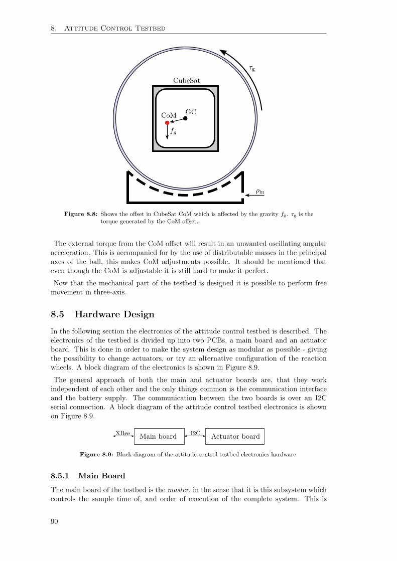
8. Attitude Control Testbed
ρin
GC
CubeSat
CoM
fg
τg
Figure 8.8: Shows the offset in CubeSat CoM which is affected by the gravity fg. τg is thetorque generated by the CoM offset.
The external torque from the CoM offset will result in an unwanted oscillating angularacceleration. This is accompanied for by the use of distributable masses in the principalaxes of the ball, this makes CoM adjustments possible. It should be mentioned thateven though the CoM is adjustable it is still hard to make it perfect.
Now that the mechanical part of the testbed is designed it is possible to perform freemovement in three-axis.
8.5 Hardware Design
In the following section the electronics of the attitude control testbed is described. Theelectronics of the testbed is divided up into two PCBs, a main board and an actuatorboard. This is done in order to make the system design as modular as possible - givingthe possibility to change actuators, or try an alternative configuration of the reactionwheels. A block diagram of the electronics is shown in Figure 8.9.
The general approach of both the main and actuator boards are, that they workindependent of each other and the only things common is the communication interfaceand the battery supply. The communication between the two boards is over an I2Cserial connection. A block diagram of the attitude control testbed electronics is shownon Figure 8.9.
Main board Actuator boardI2CXBee
Figure 8.9: Block diagram of the attitude control testbed electronics hardware.
8.5.1 Main Board
The main board of the testbed is the master, in the sense that it is this subsystem whichcontrols the sample time of, and order of execution of the complete system. This is
90

8.5. Hardware Design
done in software. The main board features a power conditioning system with under-voltage protection, Microcontroller Unit (MCU) an Inertial Measurement Unit (IMU),consisting of accelerometer, gyroscope and a magnetometer, the communication withRobot Operating System (ROS) is also performed here, this is done using an XBeemodule mounted on the main board. A block diagram of the main board subsystem isshown on Figure 8.10.
XBee
IMU
PCU
VBAT
MCU JTAGOff board I2C
USART
Figure 8.10: Blockdiagram of the main board hardware.
An important point in the attitude control testbed is that the control and determinationalgorithms is running off-board, in Matlab/Simulink and therefore the computationalcomplexity of these are not imposing on the choice of MCU, a Floating Point Unit (FPU)is therefore not necessary in the MCU. The main criteria for choosing a MCU are listedin below.
• Low power consumption
• Easy to implement
• Cost
• I2C interface
• USART Interface
Based on these criterias the Atmega2561 MCU from Atmel is chosen as main computerfor the main board. The Atmega2561 MCU has an AVR8, 8-bit Reduced InstuctionSet Computing (RISC) Harvard architecture, making it a simpler alternative than forexample a 32-bit ARM MCU. Furthermore the Atmega2561 have enough RAM andflash memory to leave room for future ideas. The AVR8 architecture is a well knownand well tested architecture, as both AAUSAT3, AAUSAT4 and AAUSAT5 flew withthis architecture in mission critical subsystems. This is not a critical system in the sensethat the systems on a satellite, but being well known make it easy to implement.
The Power Conditioning Unit (PCU) on the main board consists of a step-down switch-mode power supply, delivering 3.3 volts and up to 1.5 Ampere to all the modules of themain board. The switch-mode approach is chosen for its high efficiency compared to alinear power supply approach. The under-voltage protection in the PCU is because thatthe attitude control testbed is powered by a lithium-polymer battery. A lithium-polymerbattery can be damaged if its cells are drained below a certain level which necessitates
91

8. Attitude Control Testbed
under-voltage protection in order to protect the battery from being damaged. The powersupply simply closes down when the battery level goes below a threshold and turns onagain when charged back up to a higher threshold, introducing a hysteresis.
For attitude determination three sensors are used; a magnetometer, an accelerometerand a gyroscope. The criterias for choosing these are listed below.
• Accuracy
• Low power consumption
• Easy to implement
• Cost
Based on these criterias the MPU9250 IMU from Invensense is chosen. The MPU9250has all three sensors built into
the same package and the total current consumption when all three axes of all threesensors are in use is at 3.5 mA [Inv 14].
Pictures and schematics of the main board can be seen in Section B.1.
8.5.2 Actuator Board
The actuator board contains the drivers for both magnetic Torquers and the reactionwheels, furthermore the reaction wheels are mounted on this PCB. The actuator boardhas two functions seen from the main board; the main board can control the actuatorsvia the I2C serial interface and the main board can request the instantaneous angularvelocity of the reaction wheels. A block diagram of the hardware on the actuator boardis shown in Figure 8.11.
MAG DRV MAG
PCU
VBAT
BLDC DRV BLDC
×44×TACH
4×PWM
3×PWMMCUOff board I2C
×3
Figure 8.11: Blockdiagram of the actuator board hardware.
A central piece on the actuator board is an MCU, which serves as the point of contactfor the main board and is the controlling part for both the magnetic Torquers and thereaction wheels. An MCU for the actuator board does not need to be able to performcomplex mathematical operations due to the fact that the MCU only serves as a lowlevel controller. This controller needs to be able to control four reaction wheels and threemagnetic Torquers individually, meaning that a total of seven Pulse Width Modulation(PWM) channels are necessary. The tachometer signals from the BLDCs are in the formof pulses, where each BLDC generates three pulses per revolution, which results in theneed for four external interrupt inputs. The main criterias for choosing a MCU are listedin below.
92

8.5. Hardware Design
• Seven PWM channels
• I2C interface
• Four external interrupt inputs
• Low power consumption
• Easy to implement
• Cost
Based on these criterias the Atmega64 MCU from Atmel is chosen. The Atmega64 isbased on the same AVR8 architecture as with the MCU chosen for the main board.This match between architectures eases the implementation due to the fact that the lowlevel software drivers can be used for both MCUs. Additionally the Atmega64 MCU hasenough RAM and Flash memory to be future proof if someone in the future wanted toexperiment with running local controllers aboard the actuator board.
The PCU on the actuator board is designed similar to the PCU of the main board. Itis designed as a step-down switch-mode regulator with under-voltage protection for thelithium-polymer battery. The PCU of the actuator board delivers both 3.3 and 5 voltsand up to 1.5 Ampere per power channel.
The magnetic Torquers are driven by drivers on the actuator board. The SI9988 fullH-bridge drivers are chosen for this. The SI9988 drivers are chosen because they arewell known and well tested as they where flown on both the AAUSAT3, AAUSAT4 andAAUSAT5 missions.
The drivers for the BLDC motors are chosen based on the requirements stated in thedatasheet for the Maxon BLDC [Max 15]. Furthermore in order to simplify the interfaceto the reaction wheels a BLDC driver with a single PWM and a direction input wheredesired. The main criterias for choosing a BLDC driver are listed in below.
• A single PWM input
• A single direction pin
• Easy to implement
• Cost
Based on these main criterias the DRV10963 from Texax Industries is chosen. TheDRV10963 BLDC motor driver has a simple interface with just one PWM input andone direction pin where high/low decides which direction the motor turns, this directioncan be changed during operations. However for the reaction wheels the direction pin isfixed at a potential resulting in a counter clockwise rotational direction. The reactionwheel runs at a bias Rotations Per Minute (RPM) equalling half of their maximumrevolution speed, and hence no direction change is needed after initialisation.
Pictures and schematics of the actuator board can be seen in Section B.2.
93

8. Attitude Control Testbed
8.6 Software Design
The attitude control testbed software is comprised of three parts: the software on themain board, actuator board and the computer side interface to the embedded system.The software in the embedded systems; main and actuator boards are written in theC programming language, and the computer side software is written in the Pythonlanguage. In the following, these three parts will be described. A block diagram of themain software parts can be observed in Figure 8.12.
PythonROS
Main boardXBee
Actuator boardI2C
Figure 8.12: Block diagram of the general software of the testbed.
The main software parts shown in Figure 8.12, spans over three different “computers”,illustrated by the dashed lines; on the actuator and main board, the software is runningon an embedded processor and the Python part is running on a PC, which may alsobe running the control and estimation algorithms. For this implementation, this is thecase. The general flow of the attitude control testbed is; that the main board sends asample of sensor measurements and reaction wheels angular velocity to the embeddedsystem interface and hence Matlab/Simulink, this is then processed and a set of controlinputs for the reaction wheels is generated and sent back to the main board where thisis applied. Matlab/Simulink does not do anything between the arrival of a new set ofsensor and angular velocity measurements.
8.6.1 Embedded System Interface
The software on the PC side of the attitude control testbed is in charge of thecommunication with the embedded electronics. It then serves as an interface between,in this case, Matlab/Simulink on one side and the embedded system. This interface isimplemented as a ROS node written in the Python language. ROS is a meta-operatingsystem for robots; meta-operating system in the sense that it is a layer which is installedon top of a another operating system. A ROS network is built of a number of differentROS nodes, written in C++ or Python. A ROS node is a process that, when it initialisesit, announces itself to the ROS master and are given an identity on the network. ROSnodes communicates through a publish/subscribe message passing system, over a topic.A topic is the ROS terminology for a communication channel, all nodes in the networkcan publish or subscribe to a topic. A ROS network can span over several physicalcomputers, making ROS a highly modular and flexible approach to controlling robots,or as in this case giving a bridge to an embedded system. This capability to spanover several physical computers, can give access to the attitude control testbed withoutconnecting to the physical system, by dedicating a computer to the testbed.
The approach of using ROS as a communication interface enables, Matlab/Simulinkor any other software suites which is able to connect to a ROS network, to use thetestbed. This implements the idea of a general testbed mentioned in Section 8.1. The
94

8.6. Software Design
publish/subscribe communication pattern provided by ROS, simplifies the ApplicationProgramming Interface (API) to the testbed. This API results in, a transparent - fromthe controller/estimators point of view - connection to the sensors and actuators of thehardware.
8.6.2 Main Board
The main board is the subsystem which controls the sampling time and the timing of thedifferent jobs in the overall system. The general flow of the overall system is obtained bythe main board. This is achieved by making this board, the master in the sense that it isthis subsystem, which initiates communication with, both the PC side software and theactuator board. In order to ensure a deterministic sample time of the system, a Real-Time Operating System (RTOS) is implemented. For this the RTOS KRNL [Nielsen 16]is used. A block diagram of the software with the threads is shown in Figure 8.13.
KRNL
COMControl
SENS
ACT XBeeSET
SENS/RW
Figure 8.13: Block diagram of the software within the main board.
In the main board software there are two threads of equal priority; one forcommunication with the PC, denoted COM in Figure 8.13, side software and one forreading the IMU and controlling the actuator board, denoted Control in Figure 8.13. Forthreads of equal priority KRNL uses a pre-emptive prioritised round robin schedulingalgorithm, ensuring a deterministic sampling time for the attitude control testbed[Nielsen 16]. The communication between these two threads is performed through twoglobally defined structs, one for relaying set point from the communication thread to thecontrol thread, denoted SET in Figure 8.13 and one for the sensor reading combined withthe angular velocities of the reaction wheels, denoted SENS/RW in Figure 8.13. Boththese structs are protected by binary semaphores in order to prevent race conditions. Thescheduler runs at 100 Hz; where each thread checks for new data. The communicationthread polls for new messages from the PC, when new control values are received, theyare relayed to the control thread, and when there are new sensor measurements they arerelayed to the PC. The control task performs sensor readings with a 10 Hz sample rate,sensors readings contains both IMU and reaction wheels angular velocity, and relay themto the communication thread. When the control thread receives new reaction wheels setpoints they are relayed to the actuator board.
The control thread is therefore the responsible for the testbed running at a sample rateof 10 Hz.
95

8. Attitude Control Testbed
8.6.3 Actuator Board
As previously mentioned the actuator board functions as a slave to the main board. Thesoftware of the actuator board is in charge of three things:
• Handling the tachometer pulses from the reaction wheels
• Controlling the reaction wheels
• Controlling the magnetic Torquers
• Communication with the main board
This is accomplished by implementing the software of the actuator board as a FiniteState Machine (FSM). The states are: IDLE, GET_RPM and SET_RPM. A state transitiondiagram of the FSM is shown in Figure 8.14.
SETRPM
IDLE
GETRPMS1
S2
S3
S4
Figure 8.14: Actuator board state machine.
The state transition conditions S1 to S4 are:
S1: When the actuator board receives an order to fetch the angular velocities of thereaction wheels.
S2: When the angular velocities has been read and send back to the main board.
S3: When the actuator board receives an order adjust the control values of the reactionwheels.
S4: When the reaction wheels control values has been adjusted.
When the actuator board is powered up, it while initially go into the IDLE state. Whena command from the main board is received the actuator board will perform a statetransition based on the state transition conditions. In the state GET_RPM, the softwarereturns values, to the main broad, representing the current angular velocity of each of thereaction wheels, before transitioning back to the IDLE state, waiting for new commands.When a command for setting the angular velocities of the reaction wheels, along withset points, are received; the FSM transitions to the SET_RPM state, where the angular
96

8.6. Software Design
velocities is set to the value received from the main board. The FSM transitions backto the IDLE state when this is performed successfully.
Implementing the software as an I2C slave lets the actuator board act as a slave to themain board. The tachometer pulses are handlet with external interrupts - a tachometerpulse happens three times per revolution of the reaction wheel and with four reactionwheels this generates as many tachometer pulses. A tachometer interrupt triggers anassociated interrupt service routine which increases a counter variable. This is in turnused when the main board requests the angular velocity of the reaction wheels, this ishappening in the GET_RPM state.
Control of the reaction wheels and the magnetic Torquers are done by generating aPWM for each. When a command for changing these is received, then new set pointsare received at the same time, and the value is written to a control register for theassociated PWM output.
The I2C communication with the main board is performed using an interrupt drivenI2C interface.
8.6.4 Matlab/Simulink Implementation
The purpose of the implementation in Matlab/Simulink is to provide an environmentfor which, attitude control algorithms can easily be implemented and changed duringthe research and development processes. Due to the nature of the system where thetestbed is, from a software point of view, interfaced to, as a ROS node; this couldbe in for instance the Python or Julia languages, but it is chosen to implement inMatlab/Simulink.
The Matlab/Simulink implementation for the attitude control testbed is based upon theRobotics System Toolbox from MathWorks. Furthermore the Simulink implementationis created as an extension of the AAUSAT Simulink library, along with othercontributions described in Chapter 6. A general block diagram of the implementationis shown in Figure 8.15.
ROS SubEKF
IMU calib
ACS ROS Pub
Figure 8.15: Block diagram of the Matlab/Simulink implementation of the attitude controltestbed.
Where the blocks ROS Pub and ROS Sub respectively represents where the actuatorset points is published to the ROS network and where the sensors and angular velocitiesof the reaction wheels is subscribed to from the ROS network.
From the ROS network the sensor values from magnetometer, accelerometer andgyroscope is received together with tachometers readings through the associated ROStopic. The tachometer readings is sent to the Kalman filter described in Sections 8.2.3and 8.2.4 and the sensor measurements arrives in their raw form and is sent throughtheir respective calibration blocks.
Both the EKF and the ACS is being enabled by the sensor topic; this is in orderto enforce the sample rate defined in the main board RTOS. Consequently reaction
97

8. Attitude Control Testbed
wheels set point values are published by the rate which the sensors values arrive toMatlab/Simulink.
8.7 Summary
In this chapter the design of the attitude control testbed is described. Both mechanicalend electronic hardware was described along with the software implementation. Thesoftware in the PC running the control and attitude determination algorithms and theembedded software implementation in the embedded micro-controllers in the testbed isdescribed.
98

Chapter 9Acceptance Test
During the previous chapters, the design of attitude control algorithms and the design ofthe attitude control testbed has been described. In the following chapter these designswill be tested against the requirements listed in chapter 3.
The first thing to verify against the requirements is the attitude control testbed, sincethis is the one which will be used to test the requirements of the attitude controlalgorithm.
9.1 ACS Testbed
Two sets of requirements where defined; functional requirements and requirements forthe Attitude determination. The functional requirements are not tested but verifiedthrough the design.
In the simulations of the attitude determination in Section 8.3 it was observed that theattitude determination performs within the requirements during attitudes with a roll,pitch or yaw below 90 degrees. A test with the estimator running with inputs from thesensors within the testbed is performed. This is shown in Figure 9.1.
0 10 20 30 40 50 60 70 80 900
2
4
6
8
Time [s]
Ang
ular
Err
or[d
eg]
Figure 9.1: Attitude error magnitude, ‖θ − ˆθ‖2 for a 80 degree step in yaw.
In Figure 9.1 the estimation error is shown. The estimation error is found by usinga true vector with Euler angles, θ, calculating the estimated Euler angle vector, ˆθ,
99

9. Acceptance Test
from the estimated attitude quaternion and calculating the two-norm of the differencebetween these, ‖θ − ˆθ‖2. It should be noted that the true value is calculated from rawsensor measurements because an actual true was not available, this can be expectedto induces some noise on the θ vector, and hence also the estimation error. With thisin mind there is room for improvements in the tuning of the attitude estimator. Theaccuracy requirement for the attitude estimator states that the estimator should be ableto estimate within an error of 5 deg, this performance is not completely reached butsufficient for attitude control algorithm verification.
9.2 Control algorithm
In the following the test and verification of the sliding mode attitude control algorithmare described.
During the simulations of the sliding mode control algorithm in Section 7.2, it wasshown that the sliding mode control algorithm performs well within the requirementslisted in Section 3. This will be tested in the following section using the attitude controltestbed developed and built during this thesis.
In Figure 9.2 an 80 degree step in yaw is shown.
0 10 20 30 40 50 60 70 80
−80
−60
−40
−20
0
Time [s]
Ang
le[d
eg]
RollPitchYawYaw Reference
Figure 9.2: 80 degree step in yaw, with the sliding mode control developed in Section 7.2.
The Attitude control requirements from Section 3.2.5 is listed in Table 9.1.
No. Title Description
R4.1 Accuracy Must be able to point < 10 deg.
R4.2 Slew rate Must be able to change the attitude with a slew rate> 0.0257 rad/s
R4.3 Settling time < 5 deg max. motion, 1 min.
Table 9.1: Requirements for the target tracking mode.
R4.1 Accuracy: The attitude control is required to have an accuracy of below 10 deg;in Figure 9.2 is can be seen that the attitude control is well within this requirement.
R4.2 Slew rate: The attitude control is required to be able to deliver a slew rate of> 0.0257 rad/s. From Figure 9.2 is can be seen that the control algorithm can
100

9.2. Control algorithm
rotate the testbed hardware 80 degrees in just over 30 seconds, giving a slew rateof 0.045 rad/s: This is well within the requirement.
R4.3 Settling time: The attitude control is required to be within 5 degrees of referencein less than a minute, From Figure 9.2 it can be seen that the attitude control iswithin this requirement in 29.2 seconds.
This concludes the acceptance tests of both the attitude control testbed and the slidingmode attitude control algorithm. The attitude determination of the testbed is stillmissing some work. The determination performance is sufficient, within a roll, pitchand yaw angle, below 90 degrees, but above this, the MEKF behaves erratically. Asolution has yet to be found. With a solution, and some tuning, the filter is expected toperform within the requirements.
The sliding mode control algorithm performs well and with a large margin within therequirements.
101


Chapter 10
Closure
Through the scope of this thesis, different aspects of satellite attitude control has beeninvestigated, analysed, designed and then tested. This chapter collects the conclusionsdrawn on each area from the development of the attitude control to ideas for futureimprovements.
10.1 Conclusion
Through this thesis the following conclusions has been drawn.
10.1.1 Quaternion Sliding Mode Control
The SMC designed through this thesis benefits from using a pure quaternion slidingsurface. Moreover, the SMC has taken the largest environment disturbances into accountin order to ensure stability. Through the simulations it was seen that the SMC was ableto perform target tracking. The SMC in comparison to the linear regulator was able tochange the attitude more rapid but this could have something to do with the fact thatthe linear regulator was scaled down to ensure stability of the inner and outer loop.
Summing up; both the linear and the nonlinear control algorithms performs well withinthe requirements listed for Nadir and Target tracking, and they are both able to rejectorbit disturbances, shown through simulations and for the SMC also shown in theattitude control testbed.
Moreover, it has been investigated that the Coriolis moments generated by each reactionwheel in the Tetrahedron configuration when rotation, in an inertial reference frame issufficiently small enough to be neglected in this thesis. But for a spacecraft mission withvery high attitude accuracy requirements it might be beneficial to compensate for thecoriolis moments.
10.1.2 Design of Multiplicative Extended Kalman Filter
An MEKF has been designed and simulated. The simulation showed that the non-linearestimator was able to perform within the requirements defined in chapter 3 in an areaof ±90 from the initial attitude. It was concluded that the estimator was still able tobe used in order to verify the SMC in the testbed.
103

10. Closure
10.1.3 Attitude Control Testbed
Through this thesis an attitude control testbed was designed. The testbed is able toperform friction reduced motion in all three axes. Moreover, a actuator and main boardfor telemetry, control feedback and wireless communication with a user interface hasbeen developed. This enables the use of HIL for verification of control algorithms orfuture experiments.
Even though that the testbed has the capabilities of centre of mass adjustment, perfectlymass centering was not accomplished. This results in an initial acceleration of the ballon the air baring which is to large for the actuator board to counter. The conclusion tothis problem was to only perform attitude control in the yaw axis.
10.1.4 Sliding Mode Implementation
The SMC was tested and verified by the use of the testbed. Even though the test onlywas performed in one axis the results was still sufficient enough to conclude that onthe performance on the SMC. The test showed that the controller was well within therequirements.
10.2 Future Developments
During the tests of the attitude control testbed, it was observed that the centre of massof the testbed was rather difficult to adjust, by the manual adjustment system developed,during this thesis. It is possible to adjust the mass centre to be close to the geometriccentre but it was not close enough to perform three-dimensional attitude control by theuse of reaction wheels. The reaction wheels saturate trying to overcome the gravity andfalls down, just to try again. We propose that in order to perform three-dimensionalattitude control on the testbed, an automatic adjustment system shoud be developedand implemented.
104
Bibliography
[Bak 96] Thomas Bak, Rafał Wiśniewski & Mogens Blanke. AutonomousAttitude Determination and Control System for the Ørsted Satellite.IEEE, Aerospace Application Conference, 1996.
[Bak 99] Thomas Bak. Spacecraft Attitude Determination - a MagnetometerApproach. PhD thesis, Aalborg University Denmark, 1999.
[Blanke 10] Mogens Blanke & Martin Birkelund Larsen. Lecture note in SatelliteDynamics and Control in a Quaternion Formulation, September 2010.
[Bryson 69] Bryson, A. E. & Y. C. Ho. Applied optimal control. Waltham, MA:Blaisdell, 1969.
[CalPoly 14] CalPoly. CubeSat Design Specification Rev. 13. Rapport technique,California Polytechnic State University, February 2014.
[Cappellari 76] J. O. Cappellari, C. E. Velez & A. J. Fuchs. Mathematical theory ofthe goddard trajectory determination system. NASA - Goddard SpaceFlight Center, Greenbelt, Maryland, April 1976.
[Curtis 05] Howard D. Curtis. Orbital mechanics for engineering students. ElsevierButterworth-Heinemann, 1st edition, 2005.
[Franklin 10] Gene F. Franklin, J. David Powell & Abbas Emami-Naeini. Feedbackcontrol of dynamic systems. Pearson, 6th edition, 2010.
[Grewal 08] Mohinder S. Grewal & Angus P. Andrews. Kalman filtering - theoryand practice using matlab. John Wiley & Sons, Inc., 3rd edition, 2008.
[Hoots 80] Felix R. Hoots & Ronald L. Roehrich. Models for Propagation ofNORAD Element Sets. Spacetrack Report, no. 3, December 1980.
[Humphreys 02] Todd E. Humphreys. Attitude Determination for Small Satellites withModest Pointing Constraints. Utah State University, 2002.
[Inv 14] Invensense. MPU9250 Product Specification rev. 1.0, 01 2014.
[Jensen 10] Kasper Fuglsang Jensen & Kasper Vinther. Attitude determinationand control system for aausat3. Master’s thesis, Aalborg Universitet,6 2010.
105
Bibliography
[Khalil 02] Hassan K. Khalil. Nonlinear systems. Prentice Hall, 3rd edition, 2002.
[Kuipers 02] Jack B. Kuipers. Quaternions and rotation sequences. PrincetonUniversity Press, 2002.
[Markley 03] F.Landis Markley. Multiplicative vs. Additive Filtering for SpacecraftAttitude Determination. Rapport technique, NASA Goddad SpaceFlight Center, December 2003.
[Markley 14] F. Landis Markley & John L. Crassidis. Fundamentals of spacecraftattitude determination and control. Springer, 1st edition, 2014.
[Max 15] Maxon Motor. Maxon flat motors, 04 2015.
[NASA 69a] NASA. Spacecraft gravitational torques. NASA, May 1969.
[NASA 69b] NASA. Spacecraft magnetic torques. NASA, Marts 1969.
[NASA 69c] NASA. Spacecraft radiation torques. NASA, October 1969.
[NASA 71] NASA. Spacecraft aerodynamic torques. NASA Jet PropulsionLaboratory, January 1971.
[Nielsen 16] Jens Frederik Dalsgaard Nielsen. KRNL. https://github.com/jdn-aau/krnl, 2016. V.2016052.
[Serway 14] Raymond A. Serway & John W. Jewett. Physics for scientists andengineers with modern physics. Cengage Learning, 9th edition, 2014.
[Sidi 97] Marcel J. Sidi. Spacecraft dynamics & control. Cambridge UniversityPress, 1st edition, 1997.
[Stuelpnagel 64] John Stuelpnagel. On the Parametrization of the Three-DimensionalRotation Group. SIAM Review, vol. 6, no. 4, October 1964.
[Sørensen 10] Ole Sørensen. Lecture note in Optimal Control, February 2010.
[Utkin 09] Vadim Utkin, Jürgen Guldner & Jingxin Shi. Sliding mode controlin electro-mechanical systems. Automation and Control EngineeringSeries. Taylor & Francis Group, 2nd edition, 2009.
[Wertz 95] James R. Wertz. Spacecraft attitude determination and control. KluwerAcademic Publishers, 1995.
[Wertz 99] James R. Wertz & Wiley J. Larson. Space mission analysis and design.Space Technology Library. Springer Netherlands, 1999.
[Wie 98] Bong Wie. Space vehicle dynamics and control. AIAA EducationSeries. American Institute of Aeronautics and Astronautics, Inc., 1stedition, 1998.
[Woellert 11] Kirk Woellert, Pascale Ehrenfreund, Antonio J. Ricco & HenryHertzfeld. Cubesats: Cost-effective science and technology platformsfor emerging and developing nations. Advances in Space Research,2011.
[Xia 12] Chang-Liang Xia. Permanent magnet brushless dc motor drivers andcontrols. John Wiley & Sons Singapore Pte. Ltd., 2012.
106

Appendix A
Quaternions and Rotations
A.1 Quaternions
Sources: [Wertz 95] [Markley 14] [Kuipers 02] [Stuelpnagel 64]
In this thesis, rotations are performed by the use of quaternions. Quaternions provide aconvenient method of handling three-dimensional rotations. In the following section, thebasics of quaternions are described followed by a description of the use of quaternionsfor rotations.
A quaternion is a hypercomplex number consisting of a real part and three imaginaryparts. This can be written as:
q = q4 + q1i+ q2j + q3k (A.1)
Where the imaginary numbers i, j and k can be interpreted as vectors, spanning anorthonormal basis in R3. The quaternion can be written as:
q = q4 + q = q4 +
q1q2q3
=
[qq4
](A.2)
andi2 = j2 = k2 = ijk = −1 (A.3)
Where the imaginary parts form a noncommutative ring with
ij = −ji = k
jk = −kj = i
ki = −ik = j
(A.4)
The vector part of a quaternion is called the pure quaternion.
107

A. Quaternions and Rotations
Multiplication between two quaternions are performed as
q⊗ p = (q4 + q) (p4 + p)
= q4p4 − q>p+ q4p+ p4q + q × p
=
q4 −q3 q2 q1q3 q4 −q1 q2−q2 q1 q4 q3−q1 −q2 −q3 q4
p1p2p3p4
=
p4 p3 −p2 p1−p3 p4 p1 p2p2 −p1 p4 p3−p1 −p2 −p3 p4
q1q2q3q4
(A.5)
Quaternion conjugate, norm and inverse are given as:
q∗ = q4 − q = q4 − iq1 − jq2 − kq3
|q| =√q∗ ⊗ q =
√(q4 − q)⊗ (q4 + q)
q−1 =q∗
|q|2
(A.6)
A.1.1 Rotation by Quaternions
When using a quaternion for performing rotations, a constraint is imposed on the normof a quaternion.
|q| = 1 (A.7)
A unit norm quaternion representing a rotation in R3 about a vector u, can be writtenas
q = cos
(θ
2
)+ u sin
(θ
2
), (A.8)
a vector v can then be rotated θ degrees, in positive direction of rotation, about u by
vr = q⊗[v0
]⊗ q∗ (A.9)
where vr is the rotated vector v.
If instead a vector is to be rotated from one reference frame, x, to another, y, this canbe done by
yv = q∗ ⊗[xv0
]⊗ q (A.10)
Succesive rotations is simply performed as:
yv = q∗ ⊗[xv0
]⊗ q
p∗ ⊗[yv0
]⊗ p = p∗ ⊗
(q∗ ⊗
[xv0
]⊗ q
)⊗ p
= (q⊗ p)∗ ⊗[xv0
]⊗ (q⊗ p)
(A.11)
Notice the sequence of rotations. First by q then by p.
108
A.2. Quaternion Dynamics
A rotation matrix can be constructed from a quaternion as
R (q) =
q21 − q22 − q23 + q24 2 (q1q2 + q3q4) 2 (q1q3 − q2q4)
2 (q1q2 − q3q4) −q21 + q22 − q23 + q24 2 (q2q3 + q1q4)
2 (q1q3 + q2q4) 2 (q2q3 − q1q4) −q21 − q22 + q23 + q24
(A.12)
Where R (q) is the rotation matrix constructed form q.
From a Rotation matrix R, the quaternion representing the same rotation can be foundas
q4 = ±1
2
√(1 +R11 +R22 +R33)
q1 =1
4q4(R23 −R32)
q2 =1
4q4(R31 −R13)
q3 =1
4q4(R12 −R21)
(A.13)
In cases where q4 is very small, the calculations of the rest of the quaternion becomesinaccurate. To solve this, an other solution to find the quaternion is used in terms ofRij in order to find a larger divisor [Sidi 97].
A.2 Quaternion Dynamics
For now the an angular acceleration of the satellite c ˙ω has been derived. The quaternionrepresentation of this acceleration is investigated by the second derivative of thequaternion.
As described in the satellite kinematics Section 5.1, the first derivative of the quaternionis given as
q =1
2Ω(ω)q (A.14)
alternative representation of the first derivative shows[˙qq4
]=
[−1
2 q × ω + 12q4ω
−12 q
>ω
](A.15)
The second derivative of the quaternion is then given as
¨q = −1
2˙q × ω − 1
2q × ˙ω +
1
2q4ω +
1
2q4 ˙ω (A.16)
if the quaternion kinematics in equation A.15 is used in equation A.16
¨q = −1
2
(−1
2q × ω +
1
2q4ω
)× ω
− 1
2q × ˙ω +
1
2
(−1
2q>ω
)ω +
1
2q4 ˙ω
= −1
4ω × (q × ω)− 1
2q × ˙ω − 1
4q>ωω +
1
2q4 ˙ω
(A.17)
since there is a vector triple product the following relation holds
a× (b× c) = b(a>c
)− c
(a>b
)(A.18)
109

A. Quaternions and Rotations
By using this relation in equation A.17 the following is shown
¨q = −1
4q(ω>ω
)+
1
4ω(ω>q
)− 1
2q × ˙ω
− 1
4
(ω>q
)ω +
1
2q4 ˙ω
= −1
2q × ˙ω +
1
2q4 ˙ω − 1
4q ‖ω‖22
= −1
2
[S(q)− q4I3×3
]˙ω − 1
4q ‖ω‖22
(A.19)
T(q) = −1
2
[S(q)− q4I3×3
](A.20)
q4 = −1
2˙q>ω − 1
2q> ˙ω
= −1
2
(−1
2q × ω +
1
2q4ω
)>ω − 1
2q> ˙ω
(A.21)
In order to simplify this expression further the proprieties for for a scalar triple productis used, for which following holds
a> (b× c) = (a× b)> c (A.22)
applying the propriety of the scalar triple product to equation A.21 shows
q4 =1
4q> (ω × ω)− 1
4q4ω
>ω − 1
2q> ˙ω
= −1
2q> ˙ω − 1
4q4 ‖ω‖22
(A.23)
The quaternion acceleration is now represented as a function of the dynamic equationand the current orientation
q =
[¨qq4
]=
[T(q) ˙ω − 1
4 q ‖ω‖22−1
2 q> ˙ω − 1
4q4 ‖ω‖22
](A.24)
110

Appendix B
Testbed Electronics
B.1 Main Board
In the following, pictures and schematics of the main bord is shown.
Figure B.1: Main board top. Figure B.2: Main board bottom.
111

1
1
2
2
3
3
4
4
5
5
6
6
7
7
8
8
D D
C C
B B
A A
Title
Number RevisionSize
A3
Date: 09-04-2016 Sheet ofFile: \\..\mcu.SchDoc Drawn By:
VCC1
DOUT2
DIN/CONFIG3
DIO124
RESET5
RSSI PWM/DIO106
DIO117
[reserved]8
DTR/SLEEP_RQ/DIO89
GND10 DIO4 11CTS/DIO7 12ON/SLEEP 13VREF 14Associate/DIO5 15RTS/DIO6 16AD3/DIO3 17AD2/DIO2 18AD1/DIO1 19AD0/DIO0 20J102
XBEE
VCC VCC
GND
100nFC101
GND
10nFC102
GND GND
100nC103
SCLSDA
IMU_INT
PG5 (OC0B)1
PE0 (RXD0/PCINT8/PDI)2
PE1 (TXD0/PDO)3
PE2 (XCK0/AIN0)4
PE3 (OC3A/AIN1)5
PE4 (OC3B/INT4)6
PE5 (OC3C/INT5)7
PE6 (T3/INT6)8
PE7 (ICP3/CLKO/INT7)9
PB0 (SS/PCINT0)10
PB1 (SCK/PCINT1)11
PB2 (MOSI/PCINT2)12
PB3 (MISO/PCINT3)13
PB4 (OC2A/PCINT4)14
PB5 (OC1A/PCINT5)15
PB6 (OC1B/PCINT6)16
PB7 (OC0A/OC1C/PCINT7)17
PG3 (TOSC2)18
PG4 (TOSC1)19
RESET20
VCC 21
GND 22
XTAL223
XTAL124
PD0 (SCL/INT0)25
PD1 (SDA/INT1)26
PD2 (RXD1/INT2)27
PD3 (TXD1/INT3)28
PD4 (ICP1)29
PD5 (XCK1)30
PD6 (T1)31
PD7 (T0)32
PG0 (WR)33
PG1 (RD)34
PC0 (A8) 35PC1 (A9) 36PC2 (A10) 37PC3 (A11) 38PC4 (A12) 39PC5 (A13) 40PC6 (A14) 41PC7 (A15) 42
PG2 (ALE)43
PA7 (AD7) 44PA6 (AD6) 45PA5 (AD5) 46PA4 (AD4) 47PA3 (AD3) 48PA2 (AD2) 49PA1 (AD1) 50PA0 (AD0) 51
VCC 52
GND 53
PF7 (ADC7/TDI) 54PF6 (ADC6/TDO) 55PF5 (ADC5/TMS) 56PF4 (ADC4/TCK) 57PF3 (ADC3) 58PF2 (ADC2) 59PF1 (ADC1) 60PF0 (ADC0) 61
AREF 62
GND 63
AVCC 64
U101
ATmega2561V-8AU
11 2 2
33 4 4
55 6 6
77 8 8
99 10 10
1111 12 12
1313 14 14
1515 16 16
1717 18 18
1919 20 20
2121 22 22
P102
STACK
VBATVBAT
SDASCL
VCC
10kR102
XBEE_RXXBEE_TX
GND
100nFC105
GND
XBEE_TXXBEE_RX
12
16MHz
Y101
20pFC110
20pFC111
GND GND
RESET
10kR101
100nFC104
GND
VCC
RESET
100nFC106
100nFC107
100nFC108
GND
100nFC109
1 23 45 6
P105
ICSP
PB3/MISO
PB3/MISOPB2/MOSI
PB2/MOSI
RESET
PB1/SCK
PB1/SCK
VCC
GND
PF0PF1PF2PF3PF4PF5PF6PF7
PF0 PF1PF2 PF3PF4 PF5PF6 PF7
PA0PA1PA2PA3PA4PA5PA6PA7
PA0 PA1PA2 PA3PA4 PA5PA6 PA7
PC0PC1PC2PC3PC4PC5PC6PC7
PC0 PC1PC2 PC3PC4 PC5PC6 PC7
SCLSDA
IMU_INT
2kR103
2kR104
VCC VCC
SCLSDA
GND
EXT_RXEXT_TX
123
P106
EXT_SERIAL
EXT_TXEXT_RX
GND
1 2
GND GND
PB0
PB4PB5PB6PB7
PB1/SCKPB0
PB4 PB5PB6 PB7
PB3/MISOPB2/MOSI
D101LED_ON
D102LED
D103LED
D104LED
D105LED
D106LED
D107LED
GND
68RR105
68RR106
68RR107
68RR108
68RR109
68RR110
LED0LED1LED2LED3LED4LED5 LED0 LED1 LED2 LED3 LED4 LED5
68RR111
GND
VCC
Microcrontroller
Stack Connector
Inertial Measurement Unit
XBee Communication Module
Green debug LEDs
Extra Offboard I/O Connectors w. power
ICSP
External Serial Interface
I2C Pullups
Reset Power Indicator
Main Board
MCU
1 23 45 67 89 10
P101
PORTB
1 23 45 67 89 10
P103
PORTA
1 23 45 67 89 10
P104
PORTC
VCC
VCC
GND
GND GND
VCC
RESV (VDDIO) 1
NC 2
NC 3
NC 4
NC 5
NC 6
AUX_CL7
VDDIO 8
AD0/SDO9
REGOUT10
FSYNC11
INT12
VDD13
NC 14
NC 15
NC 16
NC 17
GND18
RESV (NC) 19
RESV (GND) 20
AUX_DA21
nCS22
SCL/SCLK23
SDA/SDI24
U102
MPU9250
11
H1MountM3
11
H2MountM3
11
H3MountM3
11
H4MountM3
GNDMounting Holes
Production_no
P107
VCC
12
34
S101PBTN
no mountC112
GND
0R
R112
PIC10101
PIC10102COC101
PIC10201PIC10202
COC102
PIC10301
PIC10302COC103
PIC10401PIC10402
COC104PIC10501PIC10502
COC105
PIC10601PIC10602
COC106
PIC10701PIC10702
COC107
PIC10801PIC10802
COC108
PIC10901PIC10902
COC109
PIC11001
PIC11002COC110
PIC11101
PIC11102COC111
PIC11201PIC11202
COC112
PID10101
PID10102COD101
PID10201PID10202
COD102PID10301PID10302
COD103PID10401PID10402
COD104PID10501PID10502
COD105PID10601PID10602
COD106PID10701PID10702
COD107
PIH101
COH1
PIH201
COH2
PIH301
COH3
PIH401
COH4
PIJ10201
PIJ10202
PIJ10203
PIJ10204
PIJ10205
PIJ10206
PIJ10207
PIJ10208
PIJ10209
PIJ102010 PIJ102011
PIJ102012
PIJ102013
PIJ102014
PIJ102015
PIJ102016
PIJ102017
PIJ102018
PIJ102019
PIJ102020
COJ102
PIP10101 PIP10102
PIP10103 PIP10104
PIP10105 PIP10106
PIP10107 PIP10108
PIP10109 PIP101010
COP101
PIP10201 PIP10202
PIP10203 PIP10204
PIP10205 PIP10206
PIP10207 PIP10208
PIP10209 PIP102010
PIP102011 PIP102012
PIP102013 PIP102014
PIP102015 PIP102016
PIP102017 PIP102018
PIP102019 PIP102020
PIP102021 PIP102022
COP102PIP10301 PIP10302
PIP10303 PIP10304
PIP10305 PIP10306
PIP10307 PIP10308
PIP10309 PIP103010
COP103
PIP10401 PIP10402
PIP10403 PIP10404
PIP10405 PIP10406
PIP10407 PIP10408
PIP10409 PIP104010
COP104
PIP10501 PIP10502
PIP10503 PIP10504
PIP10505 PIP10506
COP105
PIP10601
PIP10602
PIP10603
COP106
COP107
PIR10101
PIR10102COR101
PIR10201
PIR10202COR102
PIR10301
PIR10302COR103
PIR10401
PIR10402COR104
PIR10501
PIR10502COR105
PIR10601
PIR10602COR106
PIR10701
PIR10702COR107
PIR10801
PIR10802COR108
PIR10901
PIR10902COR109
PIR11001
PIR11002COR110
PIR11101
PIR11102COR111
PIR11201 PIR11202COR112
PIS10101
PIS10102
PIS10103
PIS10104COS101
PIU10101
PIU10102
PIU10103
PIU10104
PIU10105
PIU10106
PIU10107
PIU10108
PIU10109
PIU101010
PIU101011
PIU101012
PIU101013
PIU101014
PIU101015
PIU101016
PIU101017
PIU101018
PIU101019
PIU101020
PIU101021
PIU101022
PIU101023
PIU101024
PIU101025
PIU101026
PIU101027
PIU101028
PIU101029
PIU101030
PIU101031
PIU101032
PIU101033
PIU101034
PIU101035
PIU101036
PIU101037
PIU101038
PIU101039
PIU101040
PIU101041
PIU101042
PIU101043
PIU101044
PIU101045
PIU101046
PIU101047
PIU101048
PIU101049
PIU101050
PIU101051
PIU101052
PIU101053
PIU101054
PIU101055
PIU101056
PIU101057
PIU101058
PIU101059
PIU101060
PIU101061
PIU101062
PIU101063
PIU101064
COU101
PIU10201
PIU10202
PIU10203
PIU10204
PIU10205
PIU10206
PIU10207
PIU10208
PIU10209
PIU102010
PIU102011
PIU102012
PIU102013
PIU102014
PIU102015
PIU102016
PIU102017
PIU102018
PIU102019
PIU102020
PIU102021
PIU102022
PIU102023
PIU102024
COU102
PIY10101PIY10102
COY101
PIP10601
PIU101027
NLEXT0RX
PIP10602
PIU101028
NLEXT0TX
PIC10101 PIC10201
PIC10301
PIC10401 PIC10501
PIC10601 PIC10701 PIC10801 PIC10901
PIC11001 PIC11101
PIC11201
PID10102
PID10202 PID10302 PID10402 PID10502 PID10602 PID10702
PIH101 PIH201 PIH301 PIH401
PIJ102010
PIP10109
PIP10203 PIP10204
PIP10309
PIP10409
PIP10506
PIP10603
PIS10101 PIS10103
PIU101022
PIU101053
PIU101063
PIU10209
PIU102011
PIU102018
PIU102020
PIU10106
PIU102012
NLIMU0INT
PIR10502
PIU101033NLLED0
PIR10602
PIU101034NLLED1
PIR10702
PIU101043NLLED2
PIR10802
PIU101018NLLED3
PIR10902
PIU101019NLLED4
PIR11002PIU10101
NLLED5
PIU102021
PIU102019
PIU102017
PIU102016
PIU102015
PIU102014
PIU10207
PIU10206
PIU10205
PIU10204
PIU10203
PIU10202
PIU101032
PIU101031
PIU101030
PIU101029
PIU10109
PIU10108
PIU10107
PIU10105
PIU10104
PIP102022PIP102021
PIP102020PIP102019
PIP102018PIP102017
PIP102016PIP102015
PIJ102020
PIJ102019
PIJ102018
PIJ102017
PIJ102016
PIJ102015
PIJ102014
PIJ102013
PIJ102012
PIJ102011
PIJ10209
PIJ10208
PIJ10207
PIJ10206
PIJ10205PIR10201PIJ10204
PID10701PIR11001
PID10601PIR10901
PID10501PIR10801
PID10401PIR10701
PID10301PIR10601
PID10201PIR10501
PID10101PIR11101
PIC11202
PIR11201PIU10201
PIC11102PIU101024
PIY10101
PIC11002
PIU101023
PIY10102
PIC10302PIU102010
PIP10301
PIU101051
NLPA0PIP10302
PIU101050NLPA1
PIP10303
PIU101049
NLPA2PIP10304
PIU101048NLPA3
PIP10305
PIU101047
NLPA4PIP10306
PIU101046NLPA5
PIP10307
PIU101045
NLPA6PIP10308
PIU101044NLPA7
PIP10101
PIU101010NLPB0
PIP10102
PIP10503
PIU101011
NLPB10SCK
PIP10103
PIP10504
PIU101012
NLPB20MOSI
PIP10104
PIP10501
PIU101013
NLPB30MISO
PIP10105
PIU101014NLPB4
PIP10106
PIU101015NLPB5
PIP10107
PIU101016NLPB6
PIP10108
PIU101017NLPB7
PIP10401
PIU101042
NLPC0PIP10402
PIU101041NLPC1
PIP10403
PIU101040
NLPC2PIP10404
PIU101039NLPC3
PIP10405
PIU101038
NLPC4PIP10406
PIU101037NLPC5
PIP10407
PIU101036
NLPC6PIP10408
PIU101035NLPC7
PIP10207
PIU101061
NLPF0PIP10208
PIU101060
NLPF1
PIP10209
PIU101059
NLPF2PIP102010
PIU101058
NLPF3PIP102011
PIU101057
NLPF4PIP102012
PIU101056
NLPF5
PIP102013
PIU101055
NLPF6PIP102014
PIU101054
NLPF7
PIC10402
PIP10505
PIR10101
PIS10102 PIS10104
PIU101020
NLRESET
PIP10205
PIR10401
PIU101025
PIU102023
NLSCLPIP10206
PIR10301
PIU101026
PIU102024
NLSDA
PIP10201 PIP10202NLVBAT
PIC10102 PIC10202
PIC10502
PIC10602 PIC10702 PIC10802 PIC10902
PIJ10201
PIP101010 PIP103010
PIP104010
PIP10502
PIR10102
PIR10202
PIR10302 PIR10402
PIR11102
PIR11202
PIU101021
PIU101052
PIU101062
PIU101064
PIU10208PIU102013
PIU102022
PIJ10202
PIU10102NLXBEE0RX
PIJ10203
PIU10103NLXBEE0TX

1
1
2
2
3
3
4
4
D D
C C
B B
A A
Title
Number RevisionSize
A4
Date: 09-04-2016 Sheet ofFile: \\..\pru.SchDoc Drawn By:
PGN
D1
VIN2
EN4
VIN3
SYNC5
LBO 6
LBI7
AVIN8
AGND9
FB 10
GN
D11
GN
D12
PG 13
SW 14
SW 15
PGN
D16
ThPA
D0
U201
TPS62113
GND
VBAT
1 uFC204
10 uFC203
GND
100kR203
15kR205
LBI
6.8 uH
L201
560kR201
300kR204
GND
10 uFC201
10 uFC202
GND
1MR202
680kR206
LBI
VCC
GND
2 2
Power Regulation Unit
Main Board
GND
GND
GND 1GND 2
VCC 3P201
DC_PLUG
Vcc = 3.3 VoltUndervoltage protection cut out (VtripL) = 9.5 VoltUndervoltage protection cut in (VtripH)= 10 Volt
(VtripL - 1.256)/R203 + (Vout - 1.256)/(R202 + R206) = 1.256/R2051.281/R205 + 1.281/R206 = (VtripH - 1.281)/R203
Governing equations:
PIC20101PIC20102
COC201
PIC20201PIC20202
COC202
PIC20301PIC20302 COC203
PIC20401
PIC20402COC204
PIL20101 PIL20102
COL201
PIP20101
PIP20102
PIP20103
COP201
PIR20101
PIR20102 COR201
PIR20201
PIR20202 COR202
PIR20301
PIR20302 COR203
PIR20401
PIR20402COR204
PIR20501
PIR20502 COR205PIR20601
PIR20602 COR206
PIU20100 PIU20101
PIU20102
PIU20103
PIU20104
PIU20105
PIU20106
PIU20107
PIU20108
PIU20109
PIU201010
PIU201011 PIU201012
PIU201013
PIU201014
PIU201015
PIU201016
COU201
PIC20101 PIC20201
PIC20301
PIC20401
PIP20101
PIP20102
PIR20401PIR20501
PIU20100 PIU20101
PIU20105
PIU20109
PIU201011 PIU201012 PIU201016
PIR20301
PIR20502PIR20601
PIU20107NLLBI
PIU201013PIR20201
PIR20602
PIU20106
PIR20101
PIR20402
PIU201010
PIL20101
PIU201014
PIU201015
PIC20302
PIC20402
PIP20103
PIR20302
PIU20102
PIU20103
PIU20104
PIU20108
NLVBAT
PIC20102 PIC20202
PIL20102
PIR20102 PIR20202

B. Testbed Electronics
B.2 Actuator Board
In the following, pictures and schematics of the actuator bord is shown.
Figure B.3: Actuator board top. Figure B.4: Actuator board bottom.
In Figure B.3 the top side of the actuator board is shown without the reaction wheelsmounted. The four pieces of kapton tape attached to the top side is to protect thesoldermask top from being damaged by the reaction wheel mounts when they are screwedon to the PCB. The stack connector is in the top left side of the PCB; below this isthe connections for the magnetic torquers, six LEDs for informational purpose and toauxillory power supply outputs - one 5 volt and one 3.3 volt. At the bottom middle isthe JTAG programming connector for the MCU. On the right side of the PCB - fromthe top; reset button, two connectors for two unused port of the MCU and a externalserial port. At the top of the PCB is battery connection point and the coils used in thePCU.
In Figure B.4 the bottom side of the actuator board PCB is shown. At the top right,the stack connector can be seen. At the top the two switch-mode regulators of the PCUis located. At the middle of the PCB the MCU is located.
Figure B.5: Actuator board assembled.
114

B.2. Actuator Board
The final assembly of the actuator board is shown in Figure B.5, ready for integrationwith the main board.
The schematics is shown in the next three pages, the schematics and the PCB layoutare designet in Altium Designer.
115

1
1
2
2
3
3
4
4
5
5
6
6
7
7
8
8
D D
C C
B B
A A
Title
Number RevisionSize
A3
Date: 24-04-2016 Sheet ofFile: \\..\actuator_board.SchDoc Drawn By:
11 2 2
33 4 4
55 6 6
77 8 8
99 10 10
1111 12 12
1313 14 14
1515 16 16
1717 18 18
1919 20 20
2121 22 22
P106
STACK
VBATVBAT
SCL SDA
GND GND
D107GREEN LED
68RR110
GND
4k7R102
4k7R103
SCLSDA
PF_EX_0 PF_EX_1PF_EX_2 PF_EX_3
GND1 VDD2 PWM3 EN4 OUTA 5
SA 6
SB 7
OUTB 8
U103
SI9988
GND1 VDD2 PWM3 EN4 OUTA 5
SA 6
SB 7
OUTB 8
U104
SI9988
GND1 VDD2 PWM3 EN4 OUTA 5
SA 6
SB 7
OUTB 8
U105
SI9988
GND GND
12
P104
MAG1
12
P105
MAG2
12
P107
MAG3
MAG1PWM
MAG2PWM
MAG3PWM
Magnetic Torquer Drivers
Stack Connector
Power Indicators
I2C Pullups
VCC33
VCC33 VCC33
VCC5
Actuator Board
1 3
11
H1MountM3
11
H2MountM3
11
H3MountM3
11
H4MountM3
GNDMounting Holes
Production_no
P108
10kR101
100nFC101
GND
VCC33
RESET
GND
Reset
12
34
S101PBTN
12
16MHz
Y101
20pFC106
20pFC107
GND GND
D108RED LED
150RR111
GND
VCC5
RW1PWMRW2PWMRW3PWM
RW4PWMMAG1PWMMAG2PWM
MAG3PWM
SCLSDA
LED2LED3
PEN1
PE0 (RXD0/(PDI)2
PE1 (TXD0/PDO)3
PE2 (XCK0/AIN0)4
PE3 (OC3A/AIN1)5
PE4 (OC3B/INT4)6
PE5 (OC3C/INT5)7
PE6 (T3/INT6)8
PE7 (IC3/INT7)9
PB0 (SS)10
PB1 (SCK)11
PB2 (MOSI)12
PB3 (MISO)13
PB4 (OC0)14
PB5 (OC1A)15
PB6 (OC1B)16
PB7 (OC2/OC1C)17
PG3/TOSC218
PG4/TOSC119
RESET20
VCC 21
GND 22
XTAL223
XTAL124
PD0 (SCL/INT0)25
PD1 (SDA/INT1)26
PD2 (RXD1/INT2)27
PD3 (TXD1/INT3)28
PD4 (IC1)29
PD5 (XCK1)30
PD6 (T1)31
PD7 (T2)32
PG0 (WR)33
PG1 (RD)34
PC0 (A8) 35
PC1 (A9) 36
PC2 (A10 37
PC3 (A11) 38
PC4 (A12) 39
PC5 (A13) 40
PC6 (A14) 41
PC7 (A15) 42
PG2 (ALE)43
PA7 (AD7) 44PA6 (AD6) 45PA5 (AD5) 46PA4 (AD4) 47PA3 (AD3) 48PA2 (AD2) 49PA1 (AD1) 50PA0 (AD0) 51
VCC 52
GND 53
PF7 (ADC7/TDI) 54PF6 (ADC6/TDO) 55PF5 (ADC5/TMS) 56PF4 (ADC4/TCK) 57PF3 (ADC3) 58PF2 (ADC2) 59PF1 (ADC1) 60PF0 (ADC0) 61
AREF 62
GND 63
AVCC 64
U101
ATmega64-16AU
RESET
EXT_TXEXT_RX
GND
External Serial Interface
EXT_TXEXT_RX
D101LED
D102LED
D103LED
D104LED
D105LED
D106LED
GND
68RR104
68RR105
68RR106
68RR107
68RR108
68RR109
LED0 LED1 LED2 LED3 LED4 LED5
GREEN debug LEDs
LED4LED5
100nC102
100nC103
100nC104
100nC105
PA0 PA1PA2 PA3PA4 PA5PA6 PA7
PC0 PC1PC2 PC3PC4 PC5PC6 PC7
Extra Offboard I/O Connectors w. power
1 23 45 67 89 10
P101
PORTA
1 23 45 67 89 10
P102
PORTC
GND
GND
PA0
PA2
PA4
PA6
PA1
PA3
PA5
PA7
PC0
PC2
PC4
PC6
PC1
PC3
PC5
PC7
LED0LED1
TCK1 GND 2
TDO3 VTref 4
TMS5 nSRST 6
NC7 NC 8
TDI9 GND 10
U102
AVR_JTAG
TCKTDOTMS
TDI
GND
VCC33
TCK
TDOTMS
TDIVCC33
GND
JTAG
MCU
VCC33
VCC33
M1TACHM2TACH
M3TACHM4TACH
MCU
MAG1ENMAG2ENMAG3EN
MAG1EN
MAG2EN
MAG3EN
100nC111
100nC112
100nC113
VCC5 VCC5 VCC5
GND GND GND
123
P103
EXT_SERIAL
10µFC108
10µFC109
10µFC110
Reaction WheelR113
Reaction WheelR115
Reaction WheelR114
Reaction WheelR112
Board Specific Stuff
ACS Teststand Logo
VCC5 VCC33
GND
12
P113
12
P114
Aux. PWR
CO
PIC10101PIC10102
COC101
PIC10201PIC10202
COC102
PIC10301PIC10302
COC103
PIC10401PIC10402
COC104
PIC10501PIC10502
COC105
PIC10601PIC10602
COC106PIC10701PIC10702
COC107
PIC10801
PIC10802COC108
PIC10901
PIC10902COC109
PIC11001
PIC11002COC110
PIC11101
PIC11102COC111
PIC11201
PIC11202COC112
PIC11301
PIC11302COC113
PID10101
PID10102COD101
PID10201
PID10202COD102
PID10301
PID10302COD103
PID10401
PID10402COD104
PID10501
PID10502COD105
PID10601
PID10602COD106
PID10701PID10702
COD107PID10801PID10802
COD108 PIH101
COH1
PIH201
COH2
PIH301
COH3
PIH401
COH4
PIP10101 PIP10102
PIP10103 PIP10104
PIP10105 PIP10106
PIP10107 PIP10108
PIP10109 PIP101010
COP101
PIP10201 PIP10202
PIP10203 PIP10204
PIP10205 PIP10206
PIP10207 PIP10208
PIP10209 PIP102010
COP102
PIP10301
PIP10302
PIP10303
COP103
PIP10401
PIP10402
COP104
PIP10501
PIP10502
COP105
PIP10601 PIP10602
PIP10603 PIP10604
PIP10605 PIP10606
PIP10607 PIP10608
PIP10609 PIP106010
PIP106011 PIP106012
PIP106013 PIP106014
PIP106015 PIP106016
PIP106017 PIP106018
PIP106019 PIP106020
PIP106021 PIP106022
COP106
PIP10701
PIP10702
COP107
COP108
PIP11301
PIP11302
COP113PIP11401
PIP11402
COP114
PIR10101
PIR10102COR101
PIR10201
PIR10202COR102
PIR10301
PIR10302COR103
PIR10401
PIR10402COR104
PIR10501
PIR10502COR105
PIR10601
PIR10602COR106
PIR10701
PIR10702COR107
PIR10801
PIR10802COR108
PIR10901
PIR10902COR109
PIR11001
PIR11002COR110
PIR11101
PIR11102COR111
COR112 COR113
COR114 COR115
PIS10101
PIS10102
PIS10103
PIS10104COS101
PIU10101
PIU10102
PIU10103
PIU10104
PIU10105
PIU10106
PIU10107
PIU10108
PIU10109
PIU101010
PIU101011
PIU101012
PIU101013
PIU101014
PIU101015
PIU101016
PIU101017
PIU101018
PIU101019
PIU101020
PIU101021
PIU101022
PIU101023
PIU101024
PIU101025
PIU101026
PIU101027
PIU101028
PIU101029
PIU101030
PIU101031
PIU101032
PIU101033
PIU101034
PIU101035
PIU101036
PIU101037
PIU101038
PIU101039
PIU101040
PIU101041
PIU101042
PIU101043
PIU101044
PIU101045
PIU101046
PIU101047
PIU101048
PIU101049
PIU101050
PIU101051
PIU101052
PIU101053
PIU101054
PIU101055
PIU101056
PIU101057
PIU101058
PIU101059
PIU101060
PIU101061
PIU101062
PIU101063
PIU101064
COU101
PIU10201 PIU10202
PIU10203 PIU10204
PIU10205 PIU10206
PIU10207 PIU10208
PIU10209 PIU102010
COU102
PIU10301
PIU10302
PIU10303
PIU10304 PIU10305
PIU10306
PIU10307
PIU10308
COU103
PIU10401
PIU10402
PIU10403
PIU10404 PIU10405
PIU10406
PIU10407
PIU10408
COU104
PIU10501
PIU10502
PIU10503
PIU10504 PIU10505
PIU10506
PIU10507
PIU10508
COU105
PIY10101PIY10102
COY101
PIP10301
PIU10102NLEXT0RX
PIP10302
PIU10103NLEXT0TX
PIC10101
PIC10201 PIC10301 PIC10401 PIC10501
PIC10601 PIC10701
PIC10801 PIC10901 PIC11001PIC11101 PIC11201 PIC11301
PID10102 PID10202 PID10302 PID10402 PID10502 PID10602
PID10702 PID10802PIH101 PIH201 PIH301 PIH401
PIP10109
PIP10209
PIP10303
PIP10603 PIP10604
PIP11302 PIP11402
PIS10101 PIS10103
PIU101022
PIU101053
PIU101063
PIU10202
PIU102010
PIU10301
PIU10306
PIU10307
PIU10401
PIU10406
PIU10407
PIU10501
PIU10506
PIU10507
PIR10402
PIU101059
NLLED0
PIR10502
PIU101058
NLLED1
PIR10602
PIU101029
NLLED2
PIR10702
PIU101030
NLLED3
PIR10802
PIU101031
NLLED4
PIR10902
PIU101032
NLLED5
PIU101028NLM1TACH PIU101027NLM2TACH
PIU10109NLM3TACH
PIU10108NLM4TACH
PIU101033
PIU10304
NLMAG1E\N\
PIU10106
PIU10303
NLMAG1PWM
PIU101034
PIU10404
NLMAG2E\N\
PIU10107
PIU10403
NLMAG2PWM
PIU101043
PIU10504
NLMAG3E\N\
PIU101014
PIU10503
NLMAG3PWM
PIC10602
PIU101023
PIY10102
PIC10702
PIU101024
PIY10101
PID10101PIR10401
PID10201PIR10501
PID10301PIR10601
PID10401PIR10701
PID10501PIR10801
PID10601PIR10901
PID10701PIR11001
PID10801PIR11101
PIP10401PIU10305
PIP10402PIU10308
PIP10501PIU10405
PIP10502PIU10408
PIP106011 PIP106012
PIP106013 PIP106014
PIP106015 PIP106016
PIP106017 PIP106018
PIP106019 PIP106020
PIP106021 PIP106022
PIP10701PIU10505
PIP10702PIU10508
PIU10101
PIU10104
PIU101010
PIU101011
PIU101012
PIU101013
PIU101018
PIU101019
PIU101060
PIU101061
PIU10206
PIU10207 PIU10208
PIP10101
PIU101051
NLPA0PIP10102
PIU101050
NLPA1
PIP10103
PIU101049
NLPA2PIP10104
PIU101048
NLPA3
PIP10105
PIU101047
NLPA4PIP10106
PIU101046
NLPA5
PIP10107
PIU101045
NLPA6PIP10108
PIU101044
NLPA7
PIP10201
PIU101035
NLPC0PIP10202
PIU101036
NLPC1PIP10203
PIU101037
NLPC2PIP10204
PIU101038
NLPC3
PIP10205
PIU101039
NLPC4PIP10206
PIU101040
NLPC5
PIP10207
PIU101041
NLPC6PIP10208
PIU101042
NLPC7
PIP10607NLPF0EX00
PIP10608NLPF0EX01
PIP10609NLPF0EX02
PIP106010NLPF0EX03
PIC10102
PIR10101
PIS10102 PIS10104
PIU101020NLRESET
PIU101015NLRW1PWM
PIU101016NLRW2PWM
PIU101017NLRW3PWM
PIU10105NLRW4PWM
PIP10605
PIR10201
PIU101025NLSCL
PIP10606
PIR10301
PIU101026
NLSDA
PIU101057
PIU10201
NLTCK
PIU101054
PIU10209
NLTDIPIU101055
PIU10203
NLTDOPIU101056
PIU10205
NLTMS
PIP10601 PIP10602NLVBAT
PIC10802 PIC10902 PIC11002PIC11102 PIC11202 PIC11302
PIP11301
PIR11102
PIU10302
PIU10402
PIU10502
PIC10202 PIC10302 PIC10402 PIC10502
PIP101010
PIP102010
PIP11401
PIR10102
PIR10202 PIR10302
PIR11002
PIU101021
PIU101052
PIU101062
PIU101064
PIU10204

1
1
2
2
3
3
4
4
D D
C C
B B
A A
Title
Number RevisionSize
A4
Date: 22-05-2016 Sheet ofFile: \\..\pru.SchDoc Drawn By:
PGND
1
VIN2
EN4
VIN3
SYNC5
LBO6
LBI7
AVIN8
AGND9
FB10
GND
11
GND
12
PG13
SW14
SW15
PGND
16
ThP
AD
0
U201
TPS62113
GND
VBAT
1 uFC204
GND
100kR203
15kR205
LBI
6.8uH
L201
510kR201
150kR204
GND
GND
1MR202
1MR206
LBI
GND
Power Regulation Unit
VCC5
Actuator Board
2 3
GND1
GND2
VCC3
P201
DC_PLUG
PGND
1
VIN2
EN4
VIN3
SYNC5
LBO6
LBI7
AVIN8
AGND9
FB10
GND
11
GND
12
PG13
SW14
SW15
PGND
16
ThP
AD
0
U202
TPS62111
GND
VBAT
VCC5
1 uFC208
GND
6.8uH
L202
VCC33
1M
R207
GND
10µFC202
10µFC201
10µFC203
10µFC207 10µF
C206
GND
10µFC205
100nFC209
100nFC210
VCC5 = 5 VoltUndervoltage protection cut out (VtripL) = 9.5 VoltUndervoltage protection cut in (VtripH)= 10 Volt
VCC33 = 3.3 VoltGND
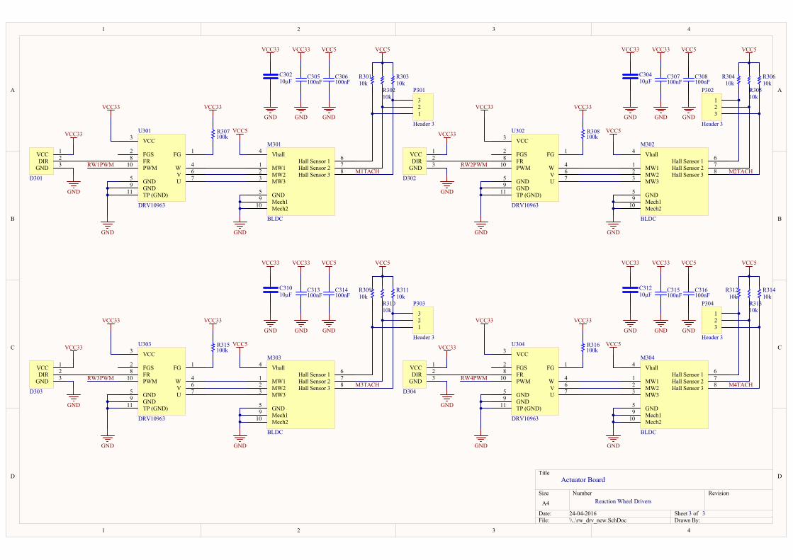
1
1
2
2
3
3
4
4
D D
C C
B B
A A
Title
Number RevisionSize
A4
Date: 24-04-2016 Sheet ofFile: \\..\rw_drv_new.SchDoc Drawn By:
GND GND
100nFC305
100nFC306
GND GND
RW1PWM
GND
100kR307
M1TACH
FG 1FGS2
VCC3
W 4
GND5 V 6
U 7
FR8
GND9
PWM10
TP (GND)11
U301
DRV10963
GND
VCC 1
DIR 2
GND 3
D301
MW11
MW22
MW33
Vhall4
GND5
Hall Sensor 1 6
Hall Sensor 2 7
Hall Sensor 3 8
Mech19
Mech210
M301
BLDC
GND GND
100nFC307
100nFC308
GND GND
RW2PWM
GND
100kR308
M2TACH
FG 1FGS2
VCC3
W 4
GND5 V 6
U 7
FR8
GND9
PWM10
TP (GND)11
U302
DRV10963
GND
VCC 1
DIR 2
GND 3
D302
MW11
MW22
MW33
Vhall4
GND5
Hall Sensor 1 6
Hall Sensor 2 7
Hall Sensor 3 8
Mech19
Mech210
M302
BLDC
GND GND
100nFC313
100nFC314
GND GND
RW3PWM
GND
100kR315
M3TACH
FG 1FGS2
VCC3
W 4
GND5 V 6
U 7
FR8
GND9
PWM10
TP (GND)11
U303
DRV10963
GND
VCC 1
DIR 2
GND 3
D303
MW11
MW22
MW33
Vhall4
GND5
Hall Sensor 1 6
Hall Sensor 2 7
Hall Sensor 3 8
Mech19
Mech210
M303
BLDC
GND GND
100nFC315
100nFC316
GND GND
RW4PWM
GND
100kR316
M4TACH
FG 1FGS2
VCC3
W 4
GND5 V 6
U 7
FR8
GND9
PWM10
TP (GND)11
U304
DRV10963
GND
VCC 1
DIR 2
GND 3
D304
MW11
MW22
MW33
Vhall4
GND5
Hall Sensor 1 6
Hall Sensor 2 7
Hall Sensor 3 8
Mech19
Mech210
M304
BLDC
VCC33 VCC33
VCC33 VCC5
VCC33 VCC33
VCC33 VCC33
VCC33
VCC33
VCC33VCC33
VCC33
VCC33
VCC33VCC33
VCC33
10kR301
10kR302
10kR303
VCC5
10kR304
10kR305
10kR306
VCC5
10kR312
10kR313
10kR314
VCC5
10kR309
10kR310
10kR311
VCC5VCC5
VCC5
VCC5
VCC5
VCC5
VCC5
VCC5
123
P303
Header 3
123
P301
Header 3
123
P302
Header 3
123
P304
Header 3
10µFC302
10µFC304
10µFC310
10µFC312
3 3
Actuator Board
Reaction Wheel Drivers
VCC33 VCC33
VCC33VCC33
PIC30201PIC30202
COC302
PIC30401PIC30402
COC304
PIC30501
PIC30502COC305
PIC30601
PIC30602COC306
PIC30701
PIC30702COC307
PIC30801
PIC30802COC308
PIC31001PIC31002
COC310
PIC31201PIC31202
COC312
PIC31301
PIC31302COC313
PIC31401
PIC31402COC314
PIC31501
PIC31502COC315
PIC31601
PIC31602COC316
PID30101
PID30102
PID30103
COD301
PID30201
PID30202
PID30203
COD302
PID30301
PID30302
PID30303
COD303
PID30401
PID30402
PID30403
COD304
PIM30101
PIM30102
PIM30103
PIM30104
PIM30105
PIM30106
PIM30107
PIM30108
PIM30109
PIM301010
COM301
PIM30201
PIM30202
PIM30203
PIM30204
PIM30205
PIM30206
PIM30207
PIM30208
PIM30209
PIM302010
COM302
PIM30301
PIM30302
PIM30303
PIM30304
PIM30305
PIM30306
PIM30307
PIM30308
PIM30309
PIM303010
COM303
PIM30401
PIM30402
PIM30403
PIM30404
PIM30405
PIM30406
PIM30407
PIM30408
PIM30409
PIM304010
COM304
PIP30101
PIP30102
PIP30103
COP301
PIP30201
PIP30202
PIP30203
COP302
PIP30301
PIP30302
PIP30303
COP303
PIP30401
PIP30402
PIP30403
COP304
PIR30101
PIR30102COR301
PIR30201
PIR30202
COR302PIR30301
PIR30302COR303
PIR30401
PIR30402COR304
PIR30501
PIR30502
COR305PIR30601
PIR30602COR306
PIR30701
PIR30702COR307
PIR30801
PIR30802COR308
PIR30901
PIR30902COR309
PIR31001
PIR31002
COR310PIR31101
PIR31102COR311
PIR31201
PIR31202COR312
PIR31301
PIR31302
COR313PIR31401
PIR31402COR314
PIR31501
PIR31502COR315
PIR31601
PIR31602COR316
PIU30101PIU30102
PIU30103
PIU30104
PIU30105
PIU30106
PIU30107
PIU30108
PIU30109
PIU301010
PIU301011
COU301
PIU30201PIU30202
PIU30203
PIU30204
PIU30205
PIU30206
PIU30207
PIU30208
PIU30209
PIU302010
PIU302011
COU302
PIU30301PIU30302
PIU30303
PIU30304
PIU30305
PIU30306
PIU30307
PIU30308
PIU30309
PIU303010
PIU303011
COU303
PIU30401PIU30402
PIU30403
PIU30404
PIU30405
PIU30406
PIU30407
PIU30408
PIU30409
PIU304010
PIU304011
COU304
PIC30201 PIC30401PIC30501 PIC30601 PIC30701 PIC30801
PIC31001 PIC31201PIC31301 PIC31401 PIC31501 PIC31601
PID30103 PID30203
PID30303 PID30403
PIM30105
PIM30109
PIM301010
PIM30205
PIM30209
PIM302010
PIM30305
PIM30309
PIM303010
PIM30405
PIM30409
PIM304010
PIU30105
PIU30109
PIU301011
PIU30205
PIU30209
PIU302011
PIU30305
PIU30309
PIU303011
PIU30405
PIU30409
PIU304011
PIM30108
PIP30103
PIR30301
NLM1TACHPIM30208
PIP30203
PIR30601
NLM2TACH
PIM30308
PIP30303
PIR31101
NLM3TACHPIM30408
PIP30403
PIR31401
NLM4TACH
PID30102 PIU30108 PID30202 PIU30208
PID30302 PIU30308 PID30402 PIU30408
PIM30101PIU30104
PIM30102PIU30106
PIM30103PIU30107
PIM30106
PIP30101
PIR30101
PIM30107
PIP30102
PIR30201
PIM30201PIU30204
PIM30202PIU30206
PIM30203PIU30207
PIM30206
PIP30201
PIR30401
PIM30207
PIP30202
PIR30501
PIM30301PIU30304
PIM30302PIU30306
PIM30303PIU30307
PIM30306
PIP30301
PIR30901
PIM30307
PIP30302
PIR31001
PIM30401PIU30404
PIM30402PIU30406
PIM30403PIU30407
PIM30406
PIP30401
PIR31201
PIM30407
PIP30402
PIR31301
PIR30701PIU30101
PIR30801PIU30201
PIR31501PIU30301
PIR31601PIU30401
PIU30102 PIU30202
PIU30302 PIU30402
PIU301010NLRW1PWM
PIU302010NLRW2PWM
PIU303010NLRW3PWM
PIU304010NLRW4PWM
PIC30602 PIC30802
PIC31402 PIC31602
PIM30104 PIM30204
PIM30304 PIM30404
PIR30102 PIR30202 PIR30302 PIR30402 PIR30502 PIR30602
PIR30902 PIR31002 PIR31102 PIR31202 PIR31302 PIR31402
PIC30202 PIC30402PIC30502 PIC30702
PIC31002 PIC31202PIC31302 PIC31502
PID30101 PID30201
PID30301 PID30401
PIR30702 PIR30802
PIR31502 PIR31602
PIU30103 PIU30203
PIU30303 PIU30403

Appendix C
Attachments
A snapshot of the attitude control testbed hardware and software is attached in thezip-file accompanying this thesis. The zip-file includes:
• acs_testbed
• space_simulator
• links to the mechanical hardware design.
In the following a short description the three parts of the attachment is given.
acs_testbed: The acs_testbed folder holds a snapshot of the repository containing:the electronic hardware diagrams with PCB layouts and the software written forthe embedded microcontrollers for both the main_board and the actuator_board.
space_simulator: The space_simulator folder holds the complete space simulatorused in this thesis. A readme file in the root of the attachment file explains howto get this up and running.
mechanical drawings: The mechanical design is performen by using Onshape, whichis an online 3D CAD software. The links leads to the 3D CAD models of theattitude control testbed.
119