dale berger hierarchical regression demonstration...

Hierarchical Regression Analysis: Gender Differences in Psychology Faculty Salaries 1

Dale Berger Hierarchical Regression Demonstration Claremont Graduate University Gender Differences in Psychology Faculty Salaries

This example demonstrates hierarchical mediation regression analysis and a bit of data cleaning.

Important lesson: If different analyses give different results, we have asked different questions.

These are real data from the APA Research Office, taken from a 2005 study of salaries of faculty

in graduate psychology programs. The original data file included only five variables: gender,

rank (lecturer through full professor), level of program where the faculty member is employed

(M.A. vs. PhD), salary, and years in rank.

Questions: Is there a gender difference in salary? Do we have evidence of sex discrimination?

The quick boilerplate analysis is an independent groups t-test.

Click Analyze, Compare Means, Independent Samples T-Test…

Select salary as the Test Variable and Sex as the Grouping Variable.

Define the levels for Sex. (1, 2). Click Paste and run the syntax.

This shows the average salary for men to be $77,188.02 and the average salary for women to be

$67,442.49, a difference of $9745.53 favoring men. The standard t-test is t = 12.65, df = 4640,

p < .001. A hasty conclusion is that female faculty members are paid 87 cents for every dollar a

male faculty member is paid for comparable work ($67,442 / $77,188 = .87).

What additional factors might account for variability in salaries? We know that people with

greater seniority generally are paid more. Perhaps faculty who teach in PhD programs are paid

more than those who teach in MA programs. We have information on these variables so we can

test to what extent these variables along with sex account for variance in individual salaries.

We should begin by examining our data and preparing the data for regression analysis. We will

begin by looking at the data. A good place to begin is with frequencies and histograms for each

of our variables. We will ask for the mean, SD, skew, kurtosis, minimum, and maximum for each

of the five variables.

Group Statistics

2803 77,188.02 27,061.030 511.132

1839 67,442.49 23,376.364 545.112

sex gender

1 Men

2 Women

salary 9-10-month salary

N Mean Std. Deviation

Std. Error

Mean

Independent Sam ples Test

54.008 .000 12.654 4640 .000 9,745.528 770.173

13.042 4306.9 .000 9,745.528 747.264

Equal variances

assumed

Equal variances

not assumed


F Sig.

Levene's Test for

Equality of Variances

t df

Sig.

(2-tailed)

Mean

Dif ference

Std. Error

Dif ference

t-test for Equality of Means

T-TEST GROUPS = sex(1 2) /MISSING = ANALYSIS /VARIABLES = salary /CRITERIA = CI(.95) .


We note that kurtosis = 3.658 for our criterion variable (salary) and the maximum value of

$261,375 is quite extreme. If the distribution of salary was normal with a mean of $73,327 and a

standard deviation of $26,101, the maximum value of 261,375 would correspond to a z-score of

(261,375 – 73,327) / 26,101 = 11.68! We have a large data set so probably our analyses will not

be very sensitive to an outlier of this magnitude, but we may wish to do some sensitivity analyses

to make sure. Possibly a log transformation of salary will produce a distribution that is much

closer to normal in shape.

Sex and Level are coded (1,2). Interpretability in regression is improved if we use dummy

coding (0,1) instead.

There are more men than women faculty in our sample, but that is not a problem for our

analyses.

There are only 84 faculty in the lecturer category. Typically these are non-tenure track positions.

We may wish to limit our analyses to tenure track positions.

Statis tics

4642 4642 4642 4642 4642

0 0 0 0 0

1.40 1.86 1.17 73,327.18 6.87

.489 .867 .377 26,101.056 4.059

.425 .440 1.748 1.594 -.188

.036 .036 .036 .036 .036

-1.820 -1.125 1.055 3.658 -1.346

.072 .072 .072 .072 .072

1 1 1 22,317 1

2 4 2 261,375 14

Valid

Missing

N

Mean

Std. Deviation

Skew ness

Std. Error of Skew ness

Kurtosis

Std. Error of Kurtosis

Minimum

Maximum

sex gender

rank

academic

rank

level

Degree level

salary

9-10-month

salary

rankyrs years

in rank

sex gender

2803 60.4 60.4 60.4

1839 39.6 39.6 100.0

4642 100.0 100.0

1 Men

2 Women

Total

Valid

Frequency Percent Valid Percent

Cumulative

Percent

rank academ ic rank

2032 43.8 43.8 43.8

1311 28.2 28.2 72.0

1215 26.2 26.2 98.2

84 1.8 1.8 100.0

4642 100.0 100.0

1 Full professor

2 Associate professor

3 Assistant professor

4 Lecturer/Instructor

Total

Valid


Cumulative

Percent


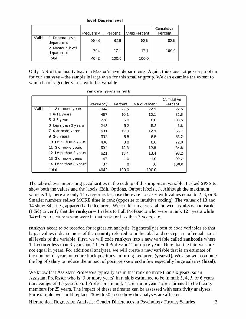
Only 17% of the faculty teach in Master’s level departments. Again, this does not pose a problem

for our analyses – the sample is large even for this smaller group. We can examine the extent to

which faculty gender varies with this variable.

The table shows interesting peculiarities in the coding of this important variable. I asked SPSS to

show both the values and the labels (Edit, Options, Output labels…). Although the maximum

value is 14, there are only 11 categories because there are no cases with values equal to 2, 3, or 8.

Smaller numbers reflect MORE time in rank (opposite to intuitive coding). The values of 13 and

14 show 84 cases, apparently the lecturers. We could run a crosstab between rankyrs and rank

(I did) to verify that the rankyrs = 1 refers to Full Professors who were in rank 12+ years while

14 refers to lecturers who were in that rank for less than 3 years, etc.

rankyrs needs to be recoded for regression analysis. It generally is best to code variables so that

larger values indicate more of the quantity referred to in the label and so steps are of equal size at

all levels of the variable. First, we will code rankyrs into a new variable called rankcode where

1=Lecturer less than 3 years and 11=Full Professor 12 or more years. Note that the intervals are

not equal in years. For additional analyses, we will create a new variable that is an estimate of

the number of years in tenure track positions, omitting Lecturers (yearstt). We also will compute

the log of salary to reduce the impact of positive skew and a few especially large salaries (lnsal).

We know that Assistant Professors typically are in that rank no more than six years, so an

Assistant Professor who is ‘3 or more years’ in rank is estimated to be in rank 3, 4, 5, or 6 years

(an average of 4.5 years). Full Professors in rank ’12 or more years’ are estimated to be faculty

members for 25 years. The impact of these estimates can be assessed with sensitivity analyses.

For example, we could replace 25 with 30 to see how the analyses are affected.

level Degree level

3848 82.9 82.9 82.9

794 17.1 17.1 100.0

4642 100.0 100.0

1 Doctoral-level

department

2 Master's-level

department

Total

Valid


Cumulative

Percent

rankyrs year s in rank

1044 22.5 22.5 22.5

467 10.1 10.1 32.6

278 6.0 6.0 38.5

243 5.2 5.2 43.8

601 12.9 12.9 56.7

302 6.5 6.5 63.2

408 8.8 8.8 72.0

594 12.8 12.8 84.8

621 13.4 13.4 98.2

47 1.0 1.0 99.2

37 .8 .8 100.0

4642 100.0 100.0

1 12 or more years

4 6-11 years

5 3-5 years

6 Less than 3 years

7 6 or more years

9 3-5 years

10 Less than 3 years

11 3 or more years


13 3 or more years


Total

Valid


Cumulative

Percent


Here is syntax that accomplishes the desired recodes:

recode sex (1=0)(2=1) into sexd. recode level (1=1)(2=0) into leveld. RECODE rankyrs (1=11)(4=10)(5=9)(6=8)(7=7)(9=6)(10=5)(11=4)(12=3)(13=2)(14=1) into rankcode. Recode rankcode (3=1.5)(4=4.5)(5=7.5)(6=10)(7=13)(8=13)(9=15)(10=19.5)(11=25)(else=sysmis) into yearstt. Compute lnsal = ln(salary). Variable labels rankcode 'Academic ranks in order' /yearstt 'Estimated years in tenure track' /lnsal = log of salary. Value labels sexd 0 'Male' 1 'Female' /leveld 0 'MA' 1 'PhD' /rankcode 1 'Lect<3' 2 'Lect3+' 3 'Asnt<3' 4 'Asnt3+' 5 'Assoc<3' 6 'Assoc3-5' 7 'Assoc6+' 8 'Full<3' 9 'Full3-5' 10 'Full6-11' 11 Full12+' .

Now, let’s conduct a regression analysis comparing men and women on salary.

Click Analyze, Regression, Linear…, select salary as the Dependent and sexd as the

Independent, click Paste and run the syntax.

Descriptive Statis tics

73,327.18 26,101.056 4642

.40 .489 4642


sexd sexd (M=0;F=1)

Mean Std. Deviation N

Cor relations

1.000 -.183

-.183 1.000

. .000

.000 .

4642 4642

4642 4642


sexd sexd (M=0;F=1)


sexd sexd (M=0;F=1)


sexd sexd (M=0;F=1)

Pearson Correlation

Sig. (1-tailed)

N

salary

9-10-month

salary

sexd sexd

(M=0;F=1)

The overall mean salary is

$73,327.18, and the sample

has 40% female faculty.

The negative correlation

indicates that people higher

on the Sex variable are

lower on salary; i.e.,

females are paid less.


The constant is the predicted value for a case where all predictors are equal to zero. In this

model, the value on sexd is zero for males, so the modeled mean salary for males is $77,188.02.

For females, sexd = 1, so we multiply the B for sexd by 1 to find that modeled salary for females

is $9,745.53 less. Compare these values to the means and other results from the initial t-test.

Now let’s limit the analysis to faculty in tenure track positions, those with rankcode > 2.

Click Data, Select cases…, select If, click If, enter rankcode > 2.

Now rerun the regression analysis.

These results are very similar, though we see the average salary is slightly higher and the

difference between males and females is slightly less.

Now we prepare to conduct a hierarchical regression analysis using sexd, leveld, and yearstt as

predictors. First, we examine the bivariate relationships and the correlations with both salary and

lnsal. What do we see in the graphs and correlation table and what are the implications?

GRAPH /SCATTERPLOT(MATRIX)=salary lnsal sex leveld yearstt /MISSING=LISTWISE . CORRELATIONS /VARIABLES=salary lnsal sexd leveld yearstt /PRINT=TWOTAIL NOSIG /MISSING=PAIRWISE .

Mode l Summ aryb

.183a .033 .033 25,664.807

Model

1

R R Square

Adjusted

R Square

Std. Error of

the Estimate

Predic tors: (Constant), sexd sexd (M=0;F=1)a.

Dependent Variable: salary 9-10-month salaryb.

Coefficientsa

77188.018 484.760 159.23 .000

-9745.528 770.173 -.183 -12.654 .000

(Constant)

sexd sexd (M=0;F=1)

Model

1

B Std. Error

Unstandardized

Coeff icients

Beta

Standardized

Coeff icients

t Sig.

Dependent Variable: salary 9-10-month salarya.

Coefficientsa

77620.087 486.138 159.667 .000

-9540.099 775.747 -.179 -12.298 .000

(Constant)

sexd sexd (M=0;F=1)

Model

1

B Std. Error

Unstandardized

Coeff icients

Beta

Standardized

Coeff icients

t Sig.

Dependent Variable: salary 9-10-month salarya.

Caution: R is always

reported as positive.

Sex predicts 3.3% of the

variance in salary.


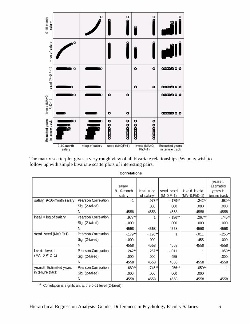
The matrix scatterplot gives a very rough view of all bivariate relationships. We may wish to

follow up with simple bivariate scatterplots of interesting pairs.

Cor relations

1 .977** -.179** .242** .689**

.000 .000 .000 .000

4558 4558 4558 4558 4558

.977** 1 -.196** .267** .745**

.000 .000 .000 .000

4558 4558 4558 4558 4558

-.179** -.196** 1 -.011 -.256**

.000 .000 .455 .000

4558 4558 4558 4558 4558

.242** .267** -.011 1 .059**

.000 .000 .455 .000

4558 4558 4558 4558 4558

.689** .745** -.256** .059** 1

.000 .000 .000 .000

4558 4558 4558 4558 4558

Pearson Correlation

Sig. (2-tailed)

N

Pearson Correlation

Sig. (2-tailed)

N

Pearson Correlation

Sig. (2-tailed)

N

Pearson Correlation

Sig. (2-tailed)

N

Pearson Correlation

Sig. (2-tailed)

N


lnsal = log of salary

sexd sexd (M=0;F=1)

leveld leveld

(MA=0;PhD=1)

yearstt Estimated years

in tenure track

salary

9-10-month

salary

lnsal = log

of salary

sexd sexd

(M=0;F=1)

leveld leveld

(MA=0;PhD=1)

yearstt

Estimated

years in

tenure track

Correlation is signif icant at the 0.01 level (2-tailed).**.


Look at the last three columns for the first row in the scatterplot matrix. These plots show

relationships of the predictors with salary, our initial dependent variable. Look for potential

violations of the assumptions for significance testing with regression. There may be an outlier,

but with our large sample (n = 4558) the impact of one outlier of this magnitude is likely to be

trivial. Error variances are not homogeneous for leveld or for yearstt, and there is a hint of

curvilinearity. The second row shows these same relationships with the log of salary (lnsal). This

variable seems a bit better suited for regression analysis because it shows less heteroscedasticity

and perhaps slightly better linearity. The correlation matrix confirms that the correlation with

yearstt is slightly larger with lnsal (r = .745) than with the untransformed variable salary

(r = .689). We could ask for bivariate plots to examine these relationships more closely.

Reasonable people may disagree on whether to transform salary. An advantage of staying with

the raw salary measure is that it is more intuitive and it is easier to use and explain results in the

original metric. A disadvantage is that the regression model does not fit the data quite as well and

assumptions for our statistical tests are not met as well. For example, the regression model

assumes that the error in prediction is the same for all values of the predictors, but we can see

error is larger for faculty with larger values of yearstt than those with smaller values.

A pragmatic approach is to analyze the data with different models to test the robustness of

findings. If we obtain materially the same findings with alternate models, then we can be more

confident in our conclusions and we can present the results in ways that communicate those

findings clearly. If our results differ substantially, then we need to qualify our conclusions

accordingly. The purpose of multiple analyses is to assess the sensitivity of our conclusions to

various violations of assumptions – it is NOT a search for the smallest possible p value!

We will begin with a default hierarchical model on the raw salary data. Our primary interest is in

the gender difference in faculty salary after we control for years in a tenure track job and type of

academic program. We may use a different order of entry, depending on the question we wish to

address. Entering yearstt first and leveld second, we enter sexd as our third predictor. This will

provide a test of the sex difference in salary, controlling for the other two variables. In lay terms,

what is the difference in salary for men and women who are equivalent in years on the job and

the type of institution where they teach (Ph.D. granting or M.A. only).

Model Summary

Model R R Square

Adjusted R

Square

Std. Error of the

Estimate

Change Statistics

R Square

Change F Change df1 df2

Sig. F

Change

1 .689a .475 .475 18,840.540 .475 4.119E3 1 4556 .000

2 .718b .515 .515 18,103.518 .040 379.515 1 4555 .000

3 .718c .515 .515 18,105.250 .000 .129 1 4554 .720

a. Predictors: (Constant), Estimated years in tenure track

b. Predictors: (Constant), Estimated years in tenure track, leveld (MA=0;PhD=1)

c. Predictors: (Constant), Estimated years in tenure track, leveld (MA=0;PhD=1), sexd (M=0;F=1)


The Model Summary table indicates that yearstt is a very strong predictor of salary. By itself,

years in a tenure track position accounts for 47.5% of the variance in salary (Model 1). The F

Change is 4.119E3 which is 4119! (The E3 indicates multiplication by 10 to the power of 3, or

1000.) The level of the academic program leveld accounts for another 4.0% of the variance (R

Square Change for Model 2). Most importantly for the purposes of our analysis, gender sexd

does not add any additional predictive information. In fact, the F for the test of the R squared

change is only .129 (Model 3), a bit less than what one would expect by chance (F = 1.000). On

average, for faculty in our sample with the same yearstt and leveld, women are paid $203.65

less, but the standard error on this estimate is $568.098. A 95% confidence interval for the B

weight is B ± (t)*(SEB). For B on sexd, this gives -203.650 ± (1.9605)*(568.098) or ± 1172.57.

Thus, our confidence interval ranges from -$1376 to +$698.92 for the population B value.

Similarly, the t-tests of the coefficients for Model 3 in the Coefficients table show that both

yearstt and leveld are statistically significant, but sexd is not, indicating that the first two

predictors each make unique contributions to prediction of salary, but gender does not. Model 1

in the Excluded Variables table shows that sexd did not add any useful information after yearstt

was in the model, even before leveld was added.

Interpretation: There is no statistically significant difference in salary for men and women with

the same number of years in tenure track. The correlation between sexd and yearstt is -.256

indicating that women on average have fewer years in tenure track positions.


As a sensitivity analysis, we replicate this analysis using lnsal as the dependent variable.

The findings are materially the same. Estimated years in tenure track (yearstt) is an even

stronger predictor of lnsal (r = .745), accounting for 55.4% of the variance in lnsal. Program

level (leveld) adds another 5.0%, bringing us up to an R squared value of .604. Again, sexd does

not add any additional predictive information.

Note that yearstt has a larger t-value than leveld, yet B is larger for leveld than for yearstt.

Why? Consider the scaling. The B coefficient indicates the predicted difference in lnsal for one

unit difference on the predictor. One year doesn’t add much, but yearstt acts over many years.

The beta weights are for standardized predictors, so there we see a larger weight for yearstt.

We may be satisfied with our analyses and stop here, or we may wish to explore possible

interactions among our predictors, or seek additional predictors such as academic concentration

area of the faculty members (not available in this data set). Depending on our audience and our

goals, we may present the results in text, tables, or graphics, or some combination. A basic

descriptive graphic display is likely to be especially useful.

Mode l Summary

.745a .554 .554 .20852 .554 5667.396 1 4556 .000

.777b .604 .604 .19657 .050 571.680 1 4555 .000

.777c .604 .604 .19659 .000 .435 1 4554 .510

Model

1

2

3

R

R

Square

Adjusted

R Square

Std. Error of

the Estimate

R Square

Change F Change df1 df2

Sig. F

Change

Change Statistics

Predic tors: (Constant), years tt Estimated years in tenure tracka.

Predic tors: (Constant), years tt Estimated years in tenure track, leveld leveld (MA=0;PhD=1)b.

Predic tors: (Constant), years tt Estimated years in tenure track, leveld leveld (MA=0;PhD=1), sexd sexd

(M=0;F=1)

c.

Coefficientsa

10.787 .006 1855.992 .000

.028 .000 .745 75.282 .000

10.640 .008 1290.225 .000

.028 .000 .731 78.298 .000

.186 .008 .223 23.910 .000

10.642 .009 1181.299 .000

.028 .000 .730 75.516 .000

.186 .008 .223 23.911 .000

-.004 .006 -.006 -.660 .510

(Constant)

yearstt Estimated

years in tenure track

(Constant)

yearstt Estimated


leveld leveld

(MA=0;PhD=1)

(Constant)

yearstt Estimated


leveld leveld

(MA=0;PhD=1)

sexd sexd (M=0;F=1)

Model

1

2

3

B Std. Error

Unstandardized

Coef f icients

Beta

Standardized

Coef f icients

t Sig.

Dependent Variable: lnsal = log of salarya.


If we are concerned about possible interactions with sex, we may wish to run an ANOVA

analyses on these data. We could code all of the interactions for regression analysis, but it is

much easier to use ANOVA. For this analysis we will treat rankcode as a nominal variable

rather than a continuous variable, and we will include lecturers. The regression analysis used

only one df for yearstt and so was sensitive to only the linear component of yearstt, while the

ANOVA analysis with df = 10 for rankcode is sensitive to all patterns across this variable.

UNIANOVA

salary BY sex level rankcode

/METHOD = SSTYPE(3)

/PLOT = PROFILE( rankcode*sex*level )

/DESIGN = sex level rankcode sex*rankcode sex*level rankcode*level

sex*level*rankcode .

Note that SPSS uses ‘scientific notation’ for very large (or very small) numbers, such as Sum of

Squares for the Corrected Model. The number following E refers to the number of places the

decimal point is shifted, either to the left (+) or the right (-). Thus, the Sum of Squares for the

Corrected Model (1.791E+012) is 1,791,000,000,000.

This ANOVA used Type III Sum of Squares, which shows the unique contribution of each effect

controlling for all other effects. We again see clear effects of level and rankcode, but no

evidence of a unique sex effect, and there is no interaction between sex and either rankcode or

level. However, the effects of rankcode are different for the two academic program levels. Plots

are useful to provide an understanding of the nature of these effects and interactions.

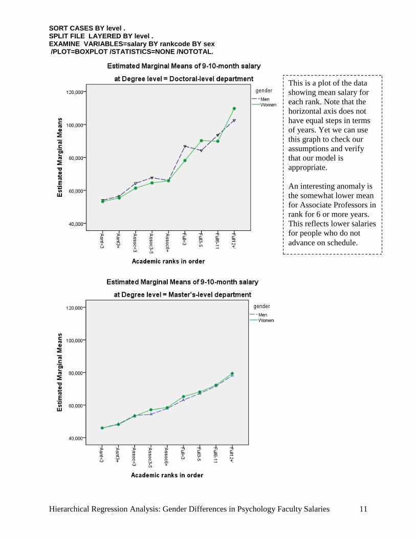
Within the SPSS chart editor, I changed the plot defaults to make the lines more distinctive, and I

changed the scales to be the same for MA and PhD levels. From the graphs it is easy to see the

strong effects of academic ranks and program level as well as the interaction between rank and

program level. The linear relationship between rank and salary is stronger in Ph.D. programs;

i.e., the difference between MA and Ph.D. salaries is greater at the higher ranks than lower ranks.

Tests of Betw een-Subjects Effects

Dependent Variable: salary 9-10-month salary

1.791E+012a 43 4.166E+010 139.750 .000

4.092E+012 1 4.092E+012 13729.683 .000

380610.332 1 380610.332 .001 .971

4.533E+010 1 4.533E+010 152.072 .000

4.925E+011 10 4.925E+010 165.229 .000

2343993697 10 234399369.7 .786 .642

29075948.4 1 29075948.37 .098 .755

2.726E+010 10 2726204021 9.146 .000

2470207217 10 247020721.7 .829 .601

1.371E+012 4598 298074787.4

2.812E+013 4642

3.162E+012 4641

Source

Corrected Model

Intercept

sex

level

rankcode

sex * rankcode

sex * level

level * rankcode

sex * level * rankcode

Error

Total

Corrected Total

Type III Sum

of Squares df Mean Square F Sig.

R Squared = .567 (Adjusted R Squared = .562)a.

!


SORT CASES BY level . SPLIT FILE LAYERED BY level . EXAMINE VARIABLES=salary BY rankcode BY sex /PLOT=BOXPLOT /STATISTICS=NONE /NOTOTAL.

This is a plot of the data

showing mean salary for

each rank. Note that the

horizontal axis does not

have equal steps in terms

of years. Yet we can use

this graph to check our

assumptions and verify

that our model is

appropriate.

An interesting anomaly is

the somewhat lower mean

for Associate Professors in

rank for 6 or more years.

This reflects lower salaries

for people who do not

advance on schedule.


Boxplots show more detail and can be very helpful for diagnostics as well as for presentations. In

default SPSS output the scales are not necessarily equal, so first impressions can be misleading.

It would look like salaries increase faster for Master’s level programs. For naive audiences, and

even for ourselves, it is good to rescale plots on the same scale if they are to be compared, as I

have done here. I double clicked on the charts in the SPSS output to edit, changing the scales so

both range from 0 to 300,000 in steps of 50,000, and I also changed the default color and texture

for one of the groups to make the two groups easier to distinguish in black and white.


The key statistical findings of the analyses are summarized in Table 1, though there is quite a bit

more that can be said about these data. In particular, the ANOVA indicates that we could do a

better job of modeling salary by including the interaction between program level and years on

the job. Also, we could do slightly better if we used the log of salary. However, for the purpose

of assessing differences in salary between men and women, the Program Level by Year on Job

interaction isn’t consequential. It is appropriate that we checked for interactions with sex and the

other predictor variables. If any interactions with sex had been present, they would impact our

conclusions about sex differences. We could include these interactions within the regression

model, but they would require coding of the interaction terms.

Table 1

Hierarchical Regression Predicting Psychology Faculty Salary with Years on Job, Academic

Program Level, and Sex (N=4558)

Final Final

Step Variable r R2 added B SEB beta

1 Years on Job .689* .475* 2127* 33.6 .676*

2 Program Level .242* .040* 13924* 715 .201*

3 Sex -.179* .000 -204 568 -.004

(Constant) 34385* 830

Cumulative R2 = .515; adjusted R

2 = .515; Program Level is coded 0 = MA, 1 = PhD; Sex is

coded 0 = Male, 1 = Female. Analysis is limited to psychology faculty in tenure track positions.

* p < .001

=====================================================================

The figures on the next page show graphical representations of a mediation model based on a

regression analysis that omits Program Level and uses arrow width to represent the relative

strength of the paths. The first figure shows standardized path coefficients and the second shows

raw B weight coefficients.

Coefficientsa

Model

Unstandardized Coefficients

Standardized

Coefficients

t Sig. B Std. Error Beta

1 (Constant) 14.873 .152 97.954 .000

sexd sexd (M=0;F=1) -4.334 .242 -.256 -17.887 .000

a. Dependent Variable: yearstt Estimated years in tenure track


Coefficientsa

Model

Unstandardized Coefficients

Standardized

Coefficients

t Sig. B Std. Error Beta

1 (Constant) 77620.087 486.138 159.667 .000

sexd sexd (M=0;F=1) -9540.099 775.747 -.179 -12.298 .000

2 (Constant) 45415.370 631.183 71.953 .000

sexd sexd (M=0;F=1) -156.114 591.224 -.003 -.264 .792

yearstt Estimated years in

tenure track

2165.339 34.945 .688 61.963 .000

a. Dependent Variable: salary 9-10-month salary

Figure 1

Standardized path coefficients showing Years in Tenure Track as a mediator of the

relationship between Sex and Salary for Tenure-track Graduate Faculty in Psychology

(N = 4558). (Direct effect is shown in parentheses.) ***p < .001

Figure 2

Unstandardized path coefficients showing Years in Tenure Track as a mediator of the

relationship between Sex and Salary for Tenure-track Graduate Faculty in Psychology

(N = 4558). (Direct effect is shown in parentheses.) ***p < .001

Sex

M=0; F=1

Years in

tenure track

Salary

.688*** -.256***

-.003

(-.179***)

(-$9540***)

- $156

$2165*** - 4.334***

years

dale berger hierarchical regression demonstration...

Documents