deep habits - columbia.edumu2166/deep_habits/res_version.pdf · ravn et al. deep habits 197 because...

Review of Economic Studies (2006) 73, 195–218 0034-6527/06/00080195$02.00c© 2006 The Review of Economic Studies Limited

Deep HabitsMORTEN RAVN

European University Institute and CEPR

STEPHANIE SCHMITT-GROHÉDuke University, CEPR, and NBER

and

MARTÍN URIBEDuke University and NBER

First version received January 2004; final version accepted June 2005 (Eds.)

This paper generalizes the standard habit-formation model to an environment in which agents formhabits over individual varieties of goods as opposed to over a composite consumption good. We refer tothis preference specification as “deep habit formation”. Under deep habits, the demand function facedby individual producers depends on past sales. This feature is typically assumed ad hoc in customer-market and brand-switching-cost models. A central result of the paper is that deep habits give rise tocountercyclical mark-ups, which is in line with the empirical evidence. This result is important, becausead hoc formulations of customer-market and switching-cost models have been criticized for implyingprocyclical and hence counterfactual mark-up movements. Under deep habits, consumption and wagesrespond procyclically to government-spending shocks. The paper provides econometric estimates of theparameters pertaining to the deep-habit model.

1. INTRODUCTION

The standard habit-persistence model, be it of the internal or external type, assumes that house-holds form habits from consumption of a single aggregate good. An important consequence ofthis assumption is that the introduction of habit formation alters the propagation of macroeco-nomic shocks only in so far as it modifies the way in which aggregate demand and possibly thesupply of labour respond to such shocks.

In this paper, we generalize the concept of habit formation by considering the possibilitythat private agents do not simply form habits from their overall consumption levels, but ratherfrom the consumption of individual goods. We have in mind an environment in which consumerscan form habits separately over narrowly defined categories of goods, such as clothing, vacationdestinations, music, cars and not just over consumption defined broadly. We believe that this de-scription of preferences, to which we refer as “deep habits”, is more compelling than its standard,or, in our terminology, “superficial”, counterpart. For example, the deep-habit formulation is em-bedded in Houthakker and Taylor’s (1970) classic work on consumption demand. Moreover, theempirical literature on consumer behaviour often finds that consumers’ choices over differentbrands of goods are affected by past brand choices (see Chintagunta, Kyriazidou and Perktold,2001, for a recent example).

The assumption that agents can form habits on a good-by-good basis has two importantimplications for aggregate dynamics. First, the demand side of the macroeconomy—in particular,the consumption Euler equation—is indistinguishable from that pertaining to an environment inwhich agents have superficial habits. Second, and more significantly, the assumption of deep-habit formation alters the supply side of the economy in fundamental ways. Specifically, when

195

196 REVIEW OF ECONOMIC STUDIES

habits are formed at the level of individual goods, firms take into account that the demand theywill face in the future depends on their current sales. This is because higher consumption of aparticular good in the current period makes consumers, all other things equal, more willing tobuy that good in the future through the force of habit. Thus, when habits are deeply rooted, theoptimal pricing problem of the firm becomes dynamic.

We embed the deep-habit-formation assumption into an economy with imperfectly competi-tive product markets. This combination results in a model of endogenous, time-varying mark-ups of prices over marginal cost. A central result of this paper is that in the deep-habit model,mark-ups behave countercyclically in equilibrium. In particular, we show that expansions inoutput driven by preference shocks, government-spending shocks, or productivity shocks areaccompanied by declines in mark-ups. This implication of the deep-habit model is in line with theempirical literature extant, which finds mark-ups to be countercyclical (Rotemberg andWoodford, 1999).

The intuition for why the deep-habit model induces countercyclical movements in mark-upsis relatively straightforward. In a simple version of the deep-habit model, the demand faced byan individual firm, say firm i , in period t is of the form qit = p−η

i t (qt − θqt−1)+ θqit−1, whereqit denotes the demand for good i , pit denotes the relative price of good i , and qt denotes thelevel of aggregate demand. Firm i takes the evolution of qt as given. The parameter θ ∈ [0,1)measures the strength of external habit for good i . This demand function is composed of twoterms. One term is p−η

i t (qt −θqt−1), displaying a price elasticity of η. The second term is θqit−1,which originates exclusively from habitual consumption of good i . Therefore, the second term isperfectly price inelastic. The price elasticity of the demand for good i is a weighted average of theelasticities of the two terms just described, namely η and 0. The weight on η is given by the shareof the price-elastic term in total demand. When aggregate demand, qt , rises, the weight of theprice-elastic term in total demand increases, and as a result the price elasticity increases. We referto this effect as the price-elasticity effect of deep habits. Because the mark-up is inversely relatedto the price elasticity of demand, it follows that under deep habits, an expansion in aggregatedemand induces a decline in mark-ups. Under either superficial habits or no habits, the demandfunction faced by firm i collapses to qit = p−η

i t qt . In this case, the price elasticity of demand forgood i is independent of the level of aggregate demand. In fact, it is constant and equal to η,implying a time-invariant mark-up.

In addition to the price-elasticity effect, deep habits influence the equilibrium dynamics ofmark-ups through an intertemporal effect. This effect arises because firms take into account thatcurrent price decisions affect future demand conditions via the formation of habits. According tothe intertemporal effect, when the present value of future per-unit profits are expected to be high,firms have an incentive to invest in customer base today. They do so by building up the currentstock of habit. In turn, this increase in habits is brought about by inducing higher current salesvia a decline in current mark-ups. The dynamic pricing problem at the level of the individualfirm that is induced by the introduction of deep external habits is akin to that studied in partialequilibrium models of customer-market pricing (Phelps and Winter, 1970) or brand-switchingcosts (Klemperer, 1995). An important difference between the deep-habit and the switching-cost/customer-market formulations is that in the deep-habit model there is gradual substitutionbetween differentiated goods rather than discrete switches among suppliers. One advantage ofthis implication of the deep-habit model, from the point of view of analytical tractability, is thatunder the deep-habit formulation one does not face an aggregation problem. In equilibrium, buy-ers can distribute their purchases identically, and still suppliers face a gradual loss of customersif they raise their relative prices. The deep-habit-formation model can therefore be viewed as anatural vehicle for incorporating switching-cost/customer-market models into a dynamic generalequilibrium framework.

RAVN ET AL. DEEP HABITS 197

Because not all components of aggregate demand may be subject to deep-habit formation, itfollows that changes in the composition of aggregate demand will, in general, affect the strengthof the aforementioned price-elasticity and intertemporal effects of deep habits on mark-ups. Forinstance, if investment spending is not subject to habit-forming behaviour, a shock that increasesthe share of investment in aggregate spending, such as an aggregate productivity shock, wouldreduce the overall importance of habits and, as a result, alter the pricing behaviour of firms.

The countercyclicality of mark-ups is a particularly interesting implication of the deep-habit model, for existing general equilibrium versions of customer-market and switching-costmodels have been criticized on the grounds that they predict procyclical mark-ups (Rotembergand Woodford, 1991, 1995). This criticism, however, is based upon customer-market models inwhich the demand function faced by individual firms is specified ad hoc and not derived fromthe optimizing behaviour of households. Our results show that once the demand for individualgoods is derived from first principles, a customer-market model is indeed capable of predictingan empirically relevant cyclical behaviour of mark-ups.

A further contribution of this paper is to estimate the structural parameters of the deepexternal habit model. Existing econometric estimates of the degree of habit formation identifythe parameters defining habits from the consumer’s Euler equation. This restriction continues tobe present in our deep-habit model. Therefore, available estimates of the degree of external habitformation can as well be interpreted as estimates of the degree of deep external habit formation.However, the deep-habit model contains additional equilibrium conditions that can be used toidentify the habit parameters, namely, supply-side restrictions stemming from the optimal pricingdecision of firms. In our econometric work, we exploit these additional identifying restrictionsto obtain more efficient estimates of the habit parameter. Our results are consistent with previousstudies, which rely solely on Euler equation estimations, in that they suggest a relatively highdegree of habit persistence and an inertial evolution of the stock of habit over time.

The remainder of the paper is organized in four sections. Section 2 develops the deep-habitmodel in the context of a simple production economy without capital. Section 3 studies the equi-librium dynamics of the deep-habit model within a fully fledged real-business-cycle environmentwith endogenous labour supply, capital accumulation, and a government sector. That section in-vestigates the response of aggregate activity, factor prices, and mark-ups to a variety of shocks.It also reports econometric estimates of the parameters of the deep-habit model. Much of the pa-per focuses on the case in which deep habits are external and additive. Section 4 considers threeimportant variations of this baseline specification. One variation is a model with good-specificsubsistence points. In this model the price-elasticity effect mentioned above stands in isolation,and the intertemporal effect is absent. The second variation studies an environment with relativedeep habits. In this economy, the price-elasticity effect is eliminated, whereas the intertempo-ral effect remains active. The third variation studies the case of internal deep habits. It showsthat when households internalize their propensity to develop addiction to individual goods, themonopolist’s pricing problem ceases to be time consistent. Section 5 concludes.

2. A SIMPLE ECONOMY WITH DEEP HABITS

Consider an economy populated by a continuum of identical households of measure 1 indexedby j ∈ [0,1]. Each household j has preferences defined over consumption of a continuum ofdifferentiated goods, c j

i t . Good varieties are indexed by i ∈ [0,1]. Households also value leisure,and thus derive disutility from labour effort, h j

t . Following Abel (1990), preferences feature“external habit formation”, or “catching up with the Joneses”. The central difference betweenAbel’s specification and ours is that we assume that consumption externalities operate at thelevel of each individual good rather than at the level of the composite final good. We refer to this


variant as “catching up with the Joneses good by good” or deep habits. Specifically, we assumethat household j derives utility from an object x j

t defined by

x jt =

⎡⎣ 1∫

0

(c ji t − θcit−1)

1−1/ηdi

⎤⎦

1/(1−1/η)

, (1)

where cit−1 ≡ ∫ 10 c j

i t−1d j denotes the cross-sectional average level of consumption of varietyi in period t − 1, which the household takes as exogenously given. The parameter θ measuresthe degree of external habit formation in consumption of each variety. When θ = 0, we havethe benchmark case of preferences displaying no consumption externalities. The parameter η > 0denotes the intratemporal elasticity of substitution of habit-adjusted consumption across differentvarieties.

For any given level of x jt , purchases of each variety i ∈ [0,1] in period t must solve the dual

problem of minimizing total expenditure,∫ 1

0 Pit cji t di , subject to the aggregation constraint (1),

where Pit denotes the nominal price of a good of variety i at time t . The optimal level of c ji t for

i ∈ [0,1] is then given by

c ji t =

(Pit

Pt

)−η

x jt + θcit−1, (2)

where Pt ≡[∫ 1

0 P1−ηi t di

]1/(1−η), is a nominal price index. Note that consumption of each variety

is decreasing in its relative price, Pit/Pt ; increasing in the level of habit-adjusted consumption,x j

t ; and for θ > 0, increasing in past aggregate consumption of the variety in question. At theoptimum, we have that Pt x

jt = ∫ 1

0 Pit (cji t − θcit−1)di .

The utility function of the household is assumed to be of the form

E0

∞∑t=0

β tU (x jt ,h j

t ), (3)

where Et denotes the mathematical expectations operator conditional on information available attime t , β ∈ (0,1) represents a subjective discount factor, and U is a period utility index assumedto be strictly increasing in its first argument, strictly decreasing in its second argument, twicecontinuously differentiable, and strictly concave.

In each period t ≥ 0, households are assumed to have access to complete contingent claimsmarkets. Let rt,t+ j denote the stochastic discount factor such that Etrt,t+ j zt+ j is the price atperiod t of a random payment zt+ j in period t + j . In addition, households are assumed to beentitled to the receipt of pure profits from the ownership of firms, �

jt . Then, the representative

household’s period-by-period budget constraint can be written as

x jt +ωt + Etrt,t+1d j

t+1 = d jt +wt h

jt +�

jt , (4)

where ωt ≡ θ∫ 1

0 (Pit/Pt )cit−1di . The variable wt denotes the real wage rate. In addition, house-holds are assumed to be subject to a borrowing constraint that prevents them from engagingin Ponzi games. The representative household’s optimization problem consists in choosing pro-cesses x j

t , h jt , and d j

t+1 so as to maximize the lifetime utility function (3) subject to (4) and

a no-Ponzi-game constraint, taking as given the processes for wt , ωt , and �jt and initial asset

holdings d j0 .

The first-order conditions associated with the household’s problem are (4),

−Uh(xjt ,h j

t )

Ux (xjt ,h j

t )= wt (5)


andUx (x

jt ,h j

t )rt,t+1 = βUx (xjt+1,h j

t+1). (6)

2.1. Firms

Each variety of goods is assumed to be produced by a monopolistically competitive firm.Equation (2) implies that aggregate demand for good i , cit ≡ ∫ 1

0 c ji t d j , is given by

cit =(

Pit

Pt

)−η

xt + θcit−1, (7)

where xt ≡ ∫ 10 x j

t d j is a measure of aggregate demand. The key implication of this demandfunction is that its price elasticity is procyclical. In effect, an increase in the level of aggregatedemand, xt , raises the relative importance of the price-elastic term (Pit/Pt )

−ηxt , and reduces therelative importance of the price-inelastic, or purely habitual, demand component, θcit−1. As aresult, the price elasticity of demand for good i faced by the monopolist increases with aggregatedemand. We refer to this effect as the price-elasticity effect of deep habits. To the extent thatmark-ups of prices over marginal costs are inversely related to the price elasticity of demand, thedeep-habit model predicts that mark-ups move countercyclically.

Each good i ∈ [0,1] is manufactured using labour as an input via the linear productiontechnology yit = At hit , where yit denotes output of good i , hit denotes labour input, and At

denotes an aggregate technology shock. Firms are assumed to be price setters, to take the actionsof all other firms as given, and to stand ready to satisfy demand at the announced prices. Formally,firm i must satisfy yit ≥ cit . Firm i’s profits in period t are given by �i t ≡ (Pit/Pt )cit −wt hit .Note that real marginal costs are equal to wt/At and are independent of scale and common acrossfirms. Nominal marginal costs are thus given by MCt = (Ptwt/At ). Let µi t denote the mark-upof prices over marginal costs charged by firm i , and µt the average mark-up charged in theeconomy, that is, µi t = Pit/MCt and µt = Pt/MCt . We can then express profits of firm i inperiod t as

�i t = µi t −1

µtci t , (8)

and the aggregate demand faced by firm i as

cit =(

µi t

µt

)−η

xt + θcit−1. (9)

The firm’s problem consists in choosing processes µi t and cit so as to maximize the presentdiscounted value of profits,

Et

∞∑j=0

rt,t+ j�i t+ j , (10)

subject to (8) and (9), given processes rt,t+ j , µt , and xt .The Lagrãngian of firm i’s problem can be written as

L= E0

∞∑t=0

r0,t

{µi t −1

µtci t +νi t

[(µi t

µt

)−η

xt + θcit−1 − cit

]},

where νi t is a Lagrãnge multiplier associated with equation (9). The first-order conditions corre-sponding to this optimization problem are (9) and


νi t = µi t −1

µt+ θ Etrt,t+1νi t+1

cit = ηνi t

(µi t

µt

)−η−1

xt .

The multiplier νi t represents the shadow value of selling an extra unit of good i in period t . Thefirst of the above optimality conditions states that the value of selling an extra unit of good i inperiod t , νi t , has two components. One is the short-run profit of a sale, given by (µi t −1)/µt . Thesecond component reflects future expected profits associated with selling an extra unit of goodi in the current period. In effect, a unit increase in sales in the current period induces, via habitformation, additional sales in the amount of θ units in the next period. The present discountedvalue of these θ additional units of sales is θ Etrt,t+1νi t+1, which is precisely the second termon the R.H.S. of the first optimality condition shown above. The second optimality conditionequates the costs and benefits of a unit increase in the relative price. The benefit is given byan increase in revenue in the amount of cit stemming from selling all intramarginal units at ahigher price. The cost is the decline in demand that the price increase induces, and is given by

η(

µi tµt

)−η−1xt , evaluated at the shadow value of sales, νi t . It is straightforward to see from the

above two optimality conditions that in the absence of habit formation (θ = 0), the mark-up isconstant and equal to η/(η−1).

We note that the pricing decisions of the monopolist are time consistent. This is because thecurrent demand is independent of future expected values of Pit/Pt . This independence of currentdemand from future expected relative prices is a consequence of our maintained assumption thatdeep habits are external. Under the alternative hypothesis that habit formation is internal, thedemand for good i in period t will depend not just on the price of good i in period t but also onfuture expected prices. This feature of demand in the internal deep-habit model in conjunctionwith the fact that past sales affect the monopolist’s current price-setting behaviour may give riseto time-inconsistency problems. We discuss the case of deep internal habits further in Section 4.3.

2.2. Equilibrium

Because all households are identical, consumption and labour supplies are invariant across in-dividuals. It follows that we can drop the superscript j from all variables. We assume that theinitial conditions cit , t = −1, are the same for all goods i ∈ [0,1]. Further, we restrict attention tosymmetric equilibria, in which all firms charge the same price. Therefore, we can also drop thesubscript i from all variables. A stationary competitive equilibrium can then be defined as a setof stationary processes {xt ,ct ,ht ,rt,t+1,wt ,νt ,µt } satisfying

xt = ct − θct−1, (11)

Ux (xt ,ht )rt,t+1 = βUx (xt+1,ht+1), (12)

wt = −Uh(xt ,ht )

Ux (xt ,ht ), (13)

µt = At

wt, (14)

ct = At ht , (15)

νt = θ Etrt,t+1νt+1 +1− 1

µt, and (16)

ct = η(ct − θct−1)νt . (17)


It is of interest to compare these equilibrium conditions to those arising from the standardhabit-formation model. That is, from a model where the single-period utility function dependson the quasi-difference between current and past consumption of the composite good as op-posed to the quasi-difference between current and past consumption of each particular variety.It is straightforward to show that the superficial-habit model shares with our deep-habit modelequilibrium conditions (11)–(15). Of particular interest is the fact that because the consumptionEuler equation (12) is common to the deep-habit model as well as to the standard superficial-habit-formation models, existing Euler-equation-based empirical estimates of the degree of habitformation can be interpreted as uncovering the degree of deep-habit persistence. Because in ourmodel the parameter θ that measures the strength of deep habits appears in equations other thanthe consumption Euler equation (12), our model provides additional identification restrictions.In Section 3.4, we exploit these additional restrictions in conjunction with the Euler equation toobtain a more efficient estimate of θ .

What sets the deep- and superficial-habit models apart is the fact that under superficialhabits, equilibrium conditions (16) and (17) are replaced by the requirement that the mark-up,µt , be constant and equal to η/(η−1). This is a significant difference. The deep-habit-formationmodel introduces a dynamic wedge between factor prices and their associated marginal products.That is, the deep-habit model gives rise to time-varying mark-ups.

2.3. The price-elasticity and intertemporal effects of deep habits

It is convenient to express the mark-up as a function of the short-run price elasticity of demandand the present value of expected per-unit future profits. The reason is that these two variablescapture the main channels through which deep habits affect mark-up dynamics. Iterating equation(16) forward, and assuming that lim j→∞ θ j Etrt,t+ jνt+ j = 0, one can express νt as the presentdiscounted value of expected future per-unit profits induced by a unit increase in current sales,that is, νt = Et

∑∞j=0 θ j rt,t+ j

(µt+ j −1µt+ j

). In turn, equation (17) implies that

νt = 1

η(1− θct−1/ct ). (18)

It follows from equation (7) that the denominator on the R.H.S. of this expression is the short-run price elasticity of demand for each particular variety of goods in equilibrium. Note that theshort-run price elasticity of demand under deep habits, η(1− θct−1/ct ), is smaller than the priceelasticity of demand in the absence of deep habits, which is given by η. Furthermore, an increasein current aggregate demand, ct , relative to habitual demand, θct−1, increases the short-run priceelasticity of demand.

Using equation (18) to eliminate νt from (16) and rearranging terms yields

µt =[

1− 1

η(1− θct−1/ct )+ θ Etrt,t+1νt+1

]−1

. (19)

This expression defines the equilibrium mark-up as a function of the short-term price elasticityof demand, η(1 − θct−1/ct ), and the present value of future per-unit profits induced by a unitincrease in current sales, θ Etrt,t+1νt+1. Clearly, all other things constant, an increase in currentaggregate demand rises the short-term price elasticity of demand, inducing a decline in equilib-rium mark-ups. This is the price-elasticity effect of deep habits on mark-ups.

At the same time, an increase in the present value of future per-unit profits causes adecline in mark-ups. This is the intertemporal effect of deep habits on mark-ups. The size ofthe intertemporal effect of deep habits is determined by two components, the discount factor


rt,t+1 and the present value of future per-unit profits, νt+1. The equilibrium mark-up is decreas-ing in the discount factor, which implies that, all else constant, a rise in the real interest rateshould be associated with an increase in the current mark-up. This is because if the real interestrate is higher, then the firm discounts future profits more, and thus has less incentives to invest inmarket share today. Also, the mark-up is decreasing in νt+1, the value of future per-unit profitsdiscounted to period t +1. The intuition for why the current mark-up is decreasing in νt+1 is thatif future per-unit profits are expected to be high, then the value of having market share in thefuture is also high, and thus there is an incentive to increase the future customer base. A highercustomer base in the future can be achieved by charging lower mark-ups today.

The implied negative relation between mark-ups and expected future profits and betweenmark-ups and the discount factor distinguishes the mark-up dynamics in the deep-habit modelfrom those implied by the implicit-collusion model of Rotemberg and Saloner (1986) and Rotem-berg and Woodford (1992). In that model, collusion among firms is sustained by the crediblethreat of reverting to a perfect competition, marginal-cost-pricing regime, in the event that anyfirm fails to abide to the terms of the implicit agreement. Thus, the maximum sustainable mark-up in the collusive equilibrium is decreasing in the short-run benefit from deviating from theimplicit collusion and increasing in the long-run benefit of staying in the collusive relationship.The benefit of cheating is an increasing function of current output, while the benefit of stickingto the implicit pricing arrangement is an increasing function of the present discounted value offuture expected profits.

If θ = 0, that is, in the absence of deep habits, both the price-elasticity and intertemporaleffects vanish, rendering the mark-up time invariant and equal to η/(η − 1). A natural next stepis to explore how the price-elasticity and intertemporal effects of deep habits affect quantita-tively the dynamics of output and mark-ups within the context of a more realistic model of themacroeconomy.

3. A FULLY FLEDGED MODEL WITH DEEP HABITS

In this section, we embed deep habits into a fully fledged dynamic general equilibrium model ofthe business cycle. The goal is to quantitatively characterize the equilibrium behaviour of mark-ups in response to a variety of aggregate demand and supply shocks. We contrast the response ofmark-ups in the model with deep habits to that arising either in models featuring no habit forma-tion, or in standard habit-formation models incorporating dynamic complementarities at the levelof aggregate consumption (i.e. superficial habits). The theoretical framework considered here isricher than the one studied in Section 2, in that it features capital accumulation, a more generalformulation of deep habits, and three sources of aggregate fluctuations: government purchases,preference, and productivity shocks. In what follows, we sketch the structure of the model, leav-ing a more detailed derivation to a separate appendix (Ravn, Schmitt-Grohé and Uribe, 2004a).

3.1. Households

Household j ∈ [0,1] is assumed to have preferences that can be described by the utility function

E0

∞∑t=0

β tU (x jt − vt ,h j

t ),

where vt is an exogenous and stochastic preference shock that follows a univariate autoregressiveprocess of the form vt = ρvvt−1 + εv

t , with ρv ∈ [0,1) and εvt distributed i.i.d. with mean 0 and

standard deviation σv . This shock is meant to capture innovations to the level of private non-business absorption.


Unlike in the simple model of Section 2, we now consider a preference specification inwhich the stock of external habit depends not only upon consumption in the previous period, butalso on consumption in all past periods. Formally, the level of habit-adjusted consumption, x j

t , isnow given by

x jt =

⎡⎣ 1∫

0

(c ji t − θsit−1)

1−1/ηdi

⎤⎦

1/(1−1/η)

,

where sit−1 denotes the stock of external habit in consuming good i in period t − 1, which isassumed to evolve over time according to the following law of motion

sit = ρsit−1 + (1−ρ)cit .

The parameter ρ ∈ [0,1) measures the speed of adjustment of the stock of external habit tovariations in the cross-sectional average level of consumption of variety i . When ρ takes thevalue 0, preferences reduce to the simple case studied in Section 2.

Households are assumed to own and invest in physical capital. At the beginning of a givenperiod t , household j owns capital in the amount of k j

t that it can rent out at the rate ut in periodt . The capital stock is assumed to evolve over time according to the following law of motion

k jt+1 = (1− δ)k j

t + i jt ,

where i jt denotes investment by household j in period t . Investment is assumed to be a composite

good produced using intermediate goods via the technology

i jt =

⎡⎣ 1∫

0

(i ji t )

1−1/ηdi

⎤⎦

1/(1−1/η)

.

Note that we do not assume any habit in the production of investment goods. However, if we wereto reinterpret our deep-habit model as a switching-cost model, then one may plausibly argue thatin fact, the aggregate investment good should depend not only on the current level of purchasesof intermediate investment goods but also on their respective past levels.

3.2. The government

In each period t ≥ 0, nominal government spending is given by Pt gt . We assume that real govern-ment expenditures, denoted by gt , are exogenous, stochastic, and follow a univariate, first-orderautoregressive process of the form ln(gt/g) = ρg ln(gt−1/g)+ ε

gt , where the innovation ε

gt dis-

tributes i.i.d. with mean 0 and standard deviation σg . The government allocates spending overintermediate goods git so as to maximize the quantity of a composite good produced with inter-mediate goods according to the relationship

xgt =

⎡⎣ 1∫

0

(git − θsgit−1)

1−1/ηdi

⎤⎦

1/(1−1/η)

.

The variable sgit denotes the stock of habit in good i and is assumed to evolve over time as

sgit = ρsg

it−1 + (1−ρ)git .

We justify our specification of the aggregator function for government consumption by assum-ing that private households value government spending in goods in a way that is separablefrom private consumption and leisure and that households derive habits on consumption of


government-provided goods. The government’s problem consists in choosing git , i ∈ [0,1], so asto maximize xg

t subject to the budget constraint∫ 1

0 Pit git ≤ Pt gt and taking as given the initialcondition git = gt , for t = −1 and all i . In solving this maximization problem, the governmenttakes as given the effect of current public consumption on the level of next period’s compositegood—that is, habits in government consumption are external. Conceivably, government habitscould be treated as internal to the government, even if they are external to their beneficiaries,namely, households. This alternative, however, is analytically less tractable.

Public spending is assumed to be fully financed by lump-sum taxation.

3.3. Firms

Each good i ∈ [0,1] is manufactured using labour and capital as inputs via the following produc-tion technology:

yit = At F(kit ,hit )−φ,

where yit denotes output of good i , kit and hit denote services of capital and labour, and φdenotes fixed costs of production.1 The variable At denotes an aggregate technology shock. Weassume that the logarithm of At follows a first-order autoregressive process ln At = ρa ln At−1 +εa

t , where εat is a white noise disturbance with standard deviation σa .

The monopolist producing good i faces the following demand function:

cit + ii t + git =(

Pit

Pt

)−η

(xt + it + xgt )+ θ(sit−1 + sg

it−1).

3.4. Estimation and calibration

We compute a log-linear approximation to the policy functions in the neighbourhood of the non-stochastic steady state of the economy. We calibrate the model to the U.S. economy. The timeunit is meant to be one-quarter. We estimate the preference parameters defining deep habits us-ing a non-linear generalized method of moments (GMM) estimator. The approach that we takeis to exploit the fact that the deep-habit parameters enter both the intertemporal consumptionEuler equation—as in superficial-habit-formation models—and the equilibrium conditions deter-mining the dynamics of the mark-up, which originate on the supply side of the economy. Thischaracteristic of the deep-habit model is particularly useful, because it allows for a more efficientestimation of the habit parameters than the standard estimates of habit parameters that are derivedsolely from the consumption Euler equation.

To facilitate estimation, we assume that utility is separable in consumption and leisure.Specifically, we assume that U (x,h) = x1−σ −1

1−σ + γ (1−h)1−χ−11−χ , where 0 < σ �= 1, 0 < χ �= 1,

and γ > 0. We use U.S. quarterly data spanning the period 1967:Q1 to 2003:Q1. For a detailedpresentation of the econometric estimation, see Ravn, Schmitt-Grohé and Uribe (2004d). Basedon our estimation, we set θ = 0·86, ρ = 0·85, η = 5·3, and σ = 2.

Following Prescott (1986), we set the preference parameter γ to ensure that in the deter-ministic steady state, households devote 20% of their time to market activities. The calibra-tion restrictions that identify the remaining structural parameters of the model are taken fromRotemberg and Woodford (1992). We follow their calibration strategy to facilitate the compar-ison of our model of endogenous mark-ups due to deep habits to their ad hoc version of the

1. The presence of fixed costs introduces increasing returns to scale in the production technology. We model fixedcosts to ensure that profits are relatively small on average, as is the case of the U.S. economy, in spite of equilibriummark-ups of prices over marginal cost significantly above 0.


customer-market model. We assume that the production function is of the Cobb–Douglas type,F(k,h) = kαh1−α; α ∈ (0,1). We set the labour share in GDP to 75%, the consumption shareto 70%, the government consumption share to 12%, the annual real interest rate to 4%, and theFrisch labour supply elasticity equal to 1·3. These restrictions imply that the capital elasticityof output in production, α, is 0·25, the depreciation rate, δ, is 0·025 per quarter, the subjectivediscount factor, β, is 0·99, and the preference parameter, χ , is 3·08.

We show in Ravn et al. (2004a) that the steady-state mark-up of price over marginal cost,µ, is given by

µ = ηm

ηm −1,

where

m ≡ (sc + sg)

[(1−βρ)(1− θ)

βθ(ρ −1)+1−βρ

]+ si ≤ 1,

where sc, sg , and si denote the steady-state shares of consumption, government purchases, andinvestment in output, respectively. Our calibration implies a somewhat high average mark-up of1·32. Note, that in the case of perfect competition, that is, when η → ∞, the mark-up convergesto unity. In the case of no deep habit, that is, when θ = 0, we have that m = 1, and the mark-upequals η/(η−1) = 1·23, which relates the mark-up to the intratemporal elasticity of substitutionacross varieties in the usual way. Because under deep habits, the parameter m is less than unity,firms have more market power under deep habits than under superficial habits. This is because,in the former formulation, firms take advantage of the fact that when agents form habits on avariety-by-variety basis, the short-run price elasticity of demand for each variety is less than η.

We set the serial correlation of all three shocks to 0·9 (i.e. ρv = ρg = ρa = 0·9). Table 1summarizes the calibration.

3.5. Aggregate dynamics

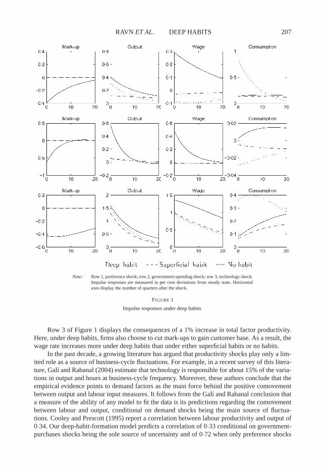
We now characterize quantitatively the response of the deep-habit model to a variety of ex-ogenous shocks. We consider three sources of aggregate fluctuations: preference shocks, vt ,government-spending shocks, gt , and productivity shocks, At . Row 1 of Figure 1 displays im-pulse responses of the mark-up, output, wages, and consumption to an increase in the preferenceshock vt in the amount of 1% of steady-state, habit-adjusted consumption. The response of thedeep-habit model is shown with a solid line. For comparison, the figure also depicts the responseof economies with superficial habit, shown with a dashed line, and no habit, shown with a dottedline.

Under all three model specifications, consumption and output increase as a result of thepreference shock. Consumption increases because the shock raises the marginal utility of con-sumption. At the same time, the shock induces an expansion in labour supply because it reducesthe value of leisure in terms of consumption. This explains why output increases in all three cases.The expansion in the supply of labour puts downward pressure on wages. In the economies withsuperficial habit or no habit, the labour demand schedule is unaffected by the preference shockon impact. In these two economies, the combination of an unchanged labour demand scheduleand an increase in the labour supply causes the equilibrium wage to fall.

By contrast, in the deep-habit model the mark-up falls significantly on impact by about0·4%. This decline in the mark-up leads to an increase in the demand for labour at any givenwage rate. This expansion in labour demand more than compensates the increase in labour sup-ply, resulting in an equilibrium increase in wages of about 0·3%. The reason why mark-ups fallin the deep-habit model is that in response to the increase in the demand for goods, the habitual,price-inelastic component of demand becomes relatively less important, making demand for each


TABLE 1

Calibration

Symbol Value Description

β 0·9902 Subjective discount factorσ 2 Inverse of intertemporal elasticity of substitutionθ 0·86 Degree of habit formationρ 0·85 Persistence of habit stockα 0·25 Capital elasticity of outputδ 0·0253 Quarterly depreciation rateη 5·3 Elasticity of substitution across varietiesεhw 1·3 Frisch elasticity of labour supplyh 0·2 Steady-state fraction of time devoted to workg 0·0318 Steady-state level of government purchasesφ 0·0853 Fixed costρv ,ρg,ρa 0·9 Persistence of exogenous shocks

individual variety of goods more price elastic. In turn, the increase in price elasticity leads firmsto cut mark-ups. This pricing strategy induces agents to form habits that firms can later on exploitby charging higher mark-ups. Summarizing, the difference between the deep-habit model and themodels with either superficial or no habit is that under deep habits the mark-up behaves counter-cyclically, and real wages are procyclical in response to an expansionary preference shock.

Row 2 of Figure 1 shows the response of the three economies under analysis to a 1% increasein government consumption. Government-spending shocks are similar to preference shocks of thetype described above in that they increase aggregate absorption and labour supply. In the case ofgovernment-spending shocks, the labour supply increases because the expansion in unproductivepublic spending leaves households poorer. The increase in labour supply introduces downwardpressure on wages. In the economies with superficial habits or no habits, the real wage indeedfalls in equilibrium. In the economy with deep habits, firms reduce mark-ups by about half a percent. The resulting expansion in labour demand is strong enough to offset the income effect onlabour supply. As a result, real wages rise in equilibrium. Thus, as in the case of innovations inprivate spending, government-purchases shocks trigger countercyclical mark-up movements andprocyclical wage movements. This finding hinges on our maintained assumption that governmentconsumption is subject to good-specific habit formation.

Of particular interest is the fact that the deep-habit model predicts that private consump-tion rises in response to an increase in government spending. In the model without deep-habitformation (with or without superficial-habit formation), private consumption spending declinesas government spending rises. This decline in consumption is driven by the negative income ef-fect introduced by higher unproductive public spending. Under deep habits, the negative incomeeffect is offset by a strong substitution effect away from leisure and into consumption inducedby the increase in wages associated with the fall in mark-ups. The positive response of privateconsumption to government-spending shocks predicted by the deep-habit model is in line withthe data, for recently, a number of authors have found that autonomous increases in governmentspending lead to higher private sector consumption (see, e.g. Fatás and Mihov, 2001; Blanchardand Perotti, 2002; and Galí, López-Salido and Vallés, 2003). In particular, Galí et al. (2003)document that for the U.S. economy, a 1% increase in government spending is followed by apersistent and significant increase in private consumption that peaks at over 0·25% after 10 quar-ters. Although the deep-habit model underpredicts the magnitude of the consumption increase,it is remarkable that it can overturn the prediction of standard neoclassical models of a negativerelationship between public and private consumption.


Note: Row 1, preference shock; row 2, government-spending shock; row 3, technology shock.Impulse responses are measured in per cent deviations from steady state. Horizontalaxes display the number of quarters after the shock.

FIGURE 1

Impulse responses under deep habits

Row 3 of Figure 1 displays the consequences of a 1% increase in total factor productivity.Here, under deep habits, firms also choose to cut mark-ups to gain customer base. As a result, thewage rate increases more under deep habits than under either superficial habits or no habits.

In the past decade, a growing literature has argued that productivity shocks play only a lim-ited role as a source of business-cycle fluctuations. For example, in a recent survey of this litera-ture, Galí and Rabanal (2004) estimate that technology is responsible for about 15% of the varia-tions in output and hours at business-cycle frequency. Moreover, these authors conclude that theempirical evidence points to demand factors as the main force behind the positive comovementbetween output and labour input measures. It follows from the Galí and Rabanal conclusion thata measure of the ability of any model to fit the data is its predictions regarding the comovementbetween labour and output, conditional on demand shocks being the main source of fluctua-tions. Cooley and Prescott (1995) report a correlation between labour productivity and output of0·34. Our deep-habit-formation model predicts a correlation of 0·33 conditional on government-purchases shocks being the sole source of uncertainty and of 0·72 when only preference shocks


are present. By contrast, the respective predicted correlations under the superficial-habit modelare −0·1 and −0·85. This finding suggests that the deep-habit model has the potential to offer abetter explanation of salient business-cycle regularities than the standard neoclassical framework,with or without superficial habits.

The predicted countercyclical behaviour of mark-ups in the deep-habit model stands in starkcontrast to ad hoc versions of switching-cost or customer-market models such as the one de-veloped in Rotemberg and Woodford (1991, 1995). For a formal quantitative comparison of thedeep-habit model and the Rotemberg and Woodford (1991, 1995) version of the customer-marketmodel, see Ravn et al. (2004d). There, we show that under all three shocks considered above, theRotemberg and Woodford customer-market model predicts that the mark-up moves in the samedirection as output. Also, in response to demand shocks, whether private or public, wages movecountercyclically.

To understand why the Rotemberg and Woodford version of the customer-market modelproduces so different a mark-up behaviour than the customer-market model based on deep-habitformation, it is important to note that in the deep-habit model the demand faced by an individualfirm features a positive, price-insensitive term, θ(sit−1 + sg

it−1), that depends only on past sales.Due to this term, the price elasticity of demand for an individual variety increases with current ag-gregate demand, providing an incentive for firms to lower mark-ups. In the Rotemberg–Woodfordcustomer-market model, there is no such price-insensitive term. As a result, the elasticity of de-mand for an individual variety is independent of current aggregate demand conditions. As wediscuss later in Section 4.2, a version of our deep-habit model in which the single-period utilityfunction depends not on the quasi-difference between current and past consumption of each va-riety but rather on the quasi-ratio of these two variables delivers a specification for the demandfunction faced by an individual firm that is closer to the one adopted ad hoc by Rotemberg andWoodford.

4. EXTENSIONS

Thus far, we have focused on an additive specification of deep habits. We identified two channelsthrough which the presence of deep habits affects mark-ups, factor prices, and aggregate activity:a static price-elasticity effect and an intertemporal effect. In the fully fledged deep-habit model ofSection 3, the price-elasticity effect of deep habits dominates the equilibrium dynamics of mark-ups in the sense that increases in aggregate demand, regardless of their origin, cause an increasein the price elasticity of the demand for each variety of goods, thereby inducing a decline inmark-ups. Here, we study two extensions of the deep-habit model that allow us to analyse theprice-elasticity and intertemporal effects in isolation. First, we shut down the intertemporal effectby considering a model with good-specific subsistence points. Second, we eliminate the price-elasticity effect, while maintaining the intertemporal effect by considering an environment withrelative deep-habit formation.

An assumption maintained up to this point is that deep habits are external to the individualconsumer. The main rational for adopting this modelling strategy is analytical convenience. Anatural extension is to consider the case in which households internalize their addictive propen-sity. We take on this task at the end of this section.

4.1. Good-specific subsistence points

In this extension, we consider a variant of the fully fledged model of Section 3 in which theintertemporal effect of deep habits vanishes, whereas the price-elasticity effect remains active.Specifically, we assume here that agents derive utility from the quasi-difference between con-


sumption of individual varieties and a good-specific subsistence point. Formally, we replace theaggregator function (1) with

x jt =

⎡⎣ 1∫

0

(c ji t − c∗

i )1−1/ηdi

⎤⎦

1/(1−1/η)

,

where c∗i is a constant subsistence level of consumption of variety i . We incorporate good-specific

subsistence points for the consumption of public goods as well. This preference specificationgives rise to an aggregate demand schedule for each individual variety of the form

cit + git + ii t = p−ηi t (xt + xg

t + it )+ c∗i + g∗

i .

For a detailed analysis of this model, see Ravn, Schmitt-Grohé and Uribe (2004c). This demandfunction shares with the one corresponding to the deep-habit model the presence of a purelyprice-inelastic term, here given by c∗

i + g∗i . As a result, the price elasticity of demand, like in the

deep-habit model, is smaller than η and procyclical. This means that the presence of good-specificsubsistence points induces a price-elasticity effect that renders the mark-up countercyclical. Asignificant difference between the good-specific subsistence-point and the deep-habit modelsis that in the former the price-inelastic term of the demand function is exogenous to the firm.Consequently, the pricing problem of the firm is static and the intertemporal effect present inthe deep-habit model ceases to exist. The good-specific subsistence-point model is, therefore,an ideal environment to study the price-elasticity effect in isolation.

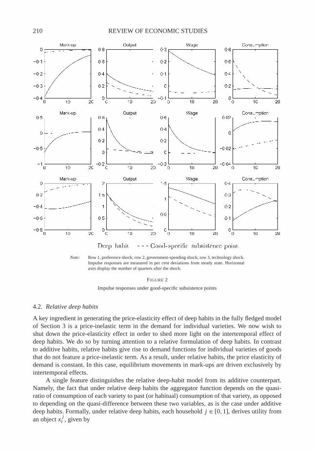
Figure 2 displays, with broken lines, the dynamics of mark-ups, wages, output, and con-sumption in response to positive preference, government-spending, and productivity shocks inthe good-specific subsistence-point model. For comparison, the figure also reproduces with solidlines the corresponding dynamics of the fully fledged deep-habits model. The calibration of thesubsistence-point model mimics that of the fully fledged, additive deep-habit model presentedin Section 3. We set the subsistence level of aggregate absorption c∗ + g∗ so that the steady-state mark-up is 32% as in the deep-habit model. The figure shows that, as expected, for allthree shocks considered, the mark-up behaves countercyclically in the good-specific subsistence-point model. However, in comparison to the deep-habit model, the mark-up movements aresmall. Indeed, the decline in mark-ups is insufficient to induce procyclical wage movements inresponse to demand shocks, a feature of the data that has been used to judge the empiricalperformance of the standard real-business-cycle model as well as alternative theories of endoge-nous mark-ups (Rotemberg and Woodford, 1992). Similarly, the good-specific subsistence-pointmodel fails to deliver a procyclical consumption response, following an increase in governmentspending, an empirical regularity stressed in Galí et al. (2003). One reason why the deep-habitand the subsistence-point models imply quantitatively such different dynamics is the fact that forgiven values of the steady-state mark-up and the parameter η, the deep-habit model features amuch larger price-inelastic component of demand. As a consequence, the price-elasticity effectis stronger in the deep-habit model than in the good-specific subsistence-point model. The rea-son why the price-inelastic component of demand is small in the good-specific subsistence-pointmodel is the absence of the intertemporal effect present in the deep-habit model. The deep-habitmodel has the ability to be consistent, both with a relatively large price-inelastic component ofdemand and a realistic average mark-up because the intertemporal effect pushes the long-runmark-up down. In turn, the reason why the intertemporal effect lowers long-run mark-ups is thatthe marginal revenue schedule that is relevant to the firm includes, in addition to the traditionalstatic marginal revenue schedule, a positive component originating in the fact that an additionalsale in the present increases sales in the future by expanding customer base through habits.



FIGURE 2

Impulse responses under good-specific subsistence points

4.2. Relative deep habits

A key ingredient in generating the price-elasticity effect of deep habits in the fully fledged modelof Section 3 is a price-inelastic term in the demand for individual varieties. We now wish toshut down the price-elasticity effect in order to shed more light on the intertemporal effect ofdeep habits. We do so by turning attention to a relative formulation of deep habits. In contrastto additive habits, relative habits give rise to demand functions for individual varieties of goodsthat do not feature a price-inelastic term. As a result, under relative habits, the price elasticity ofdemand is constant. In this case, equilibrium movements in mark-ups are driven exclusively byintertemporal effects.

A single feature distinguishes the relative deep-habit model from its additive counterpart.Namely, the fact that under relative deep habits the aggregator function depends on the quasi-ratio of consumption of each variety to past (or habitual) consumption of that variety, as opposedto depending on the quasi-difference between these two variables, as is the case under additivedeep habits. Formally, under relative deep habits, each household j ∈ [0,1], derives utility froman object x j

t , given by


x jt =

⎡⎣∫ 1

0

(c j

i t

cθi t−1

)1−1/η

di

⎤⎦

1/(1−1/η)

.

This aggregator function gives rise to an aggregate demand for each variety of goods i ∈ [0,1] ofthe form

cit =(

Pit

Pt

)−η

cθ(1−η)i t−1 xt , (20)

where Pt is a price index that firms take as exogenously given. We note that in the standardmodel without deep habits, the parameter η, denoting the intratemporal elasticity of substitutionacross varieties, must be greater than 1 in order for the monopolist problem to be well defined.We maintain this assumption here in order to be able to compare the dynamic implications ofmodels with and without deep habits. It follows that if the demand for each particular variety isto be increasing in the stock of habit (cit−1 in the simple formulation analysed here), then theparameter θ must be negative. In the numerical analysis that follows, we set θ at −0·1.2 We showelsewhere (Ravn, Schmitt-Grohé and Uribe, 2004b) that in the context of the simple economywithout capital of Section 2, the above demand function gives rise in equilibrium to a mark-up ofthe form

µt =[

1− 1

η+ θ Etrt,t+1νt+1(1−η)

ct+1

ct

]−1

. (21)

This expression is directly comparable with its counterpart in the additive deep-habit model,given by equation (19). Under relative deep habits, the price-elasticity effect of deep habits onmark-ups vanishes. This can be seen from the fact that the second term in the bracketed expres-sion, denoting the short-run price elasticity of demand, is constant and equal to 1/η. By contrast,under additive deep habits, the short-run price elasticity is procyclical, which contributes to thecountercyclicality of mark-ups. It follows that under deep relative habits the only channel throughwhich deep habits affect mark-ups is the intertemporal effect, embodied in the third term of thebracketed expression. As in the case of additive deep habits, this term represents the discountedvalue of future demand induced by an additional sale in the current period. This term is differentfrom its additive-habits counterpart in two respects. First, under additive habits, a unit increase incurrent sales raises next period’s sales by θ . Under relative habits, a unit increase in current salesraises next period’s sales by θ(1−η)ct+1/ct . As a result, under relative deep habits, an expectedincrease in the growth rate of aggregate demand induces firms to lower current mark-ups so as tobroaden their customer base. The second difference is that under relative deep habits the shadowvalue of a unit sale in period t , νt , is constant and equal to 1/η (see Ravn et al., 2004b), whereasunder additive deep habits it is time varying and countercyclical. A feature common to both therelative- and the additive-habit models is the prediction that equilibrium mark-ups increase withinterest rates (i.e. µt increases when rt,t+1 falls).

In the simple version of the relative deep-habit model analysed here, mark-ups move coun-tercyclically in response to productivity shocks (At ), but procyclically in response to shocks toprivate aggregate demand (vt ) (see figure 1 in Ravn et al., 2004b). The difference in the cyclicalbehaviour of mark-ups under supply and demand shocks is entirely driven by the dynamics ofthe interest rate. Under both types of shock, aggregate demand increases on impact and then con-verges monotonically to its steady-state position. This means that ct+1/ct is below its steady-statelevel along the entire transition. According to equation (21), this pattern of consumption growth

2. The possibility that positive values of θ give rise to counterintuitive implications for the relation between thestock of habit and the demand for goods also arises in the superficial formulation of relative habits. In effect, in this case,the marginal utility of consumption is decreasing in the stock of habit when θ is positive and the curvature of the periodutility function is less pronounced than under logarithmic preferences.


should contribute to elevated mark-up levels under both types of shock. However, under demandshocks the interest rate increases, reinforcing the rise in mark-ups, whereas under the supplyshock the real interest rate falls, offsetting the effect of consumption growth. The reason why thereal interest rate rises in response to a positive preference shock is that preference-shock-adjustedconsumption, xt − vt , falls on impact and converges monotonically to its long-run position. Inturn, the reason why the real interest rate falls in response to a positive technology shock is that,in the absence of any investment opportunities, agents must be given disincentives to save (orincentives to consume) the initial increase in output. This disincentive takes the form of low realinterest rates.

Consider now, the effects of relative deep habits in the fully fledged model with capitalaccumulation and government purchases presented in Section 3. In this model, the aggregatedemand for each variety of goods i ∈ [0,1] faced by a monopolist is given by:

cit + git + ii t =(

Pit

Pt

)−η

xt sθ(1−η)i t−1 +

(Pit

Pgt

)−η

xgt [sg

it−1]θ(1−η) + Pit

Pt

−η

it ,

where Pt , Pgt , and Pt denote price indices of habit-adjusted private consumption, habit-adjusted

public consumption, and private investment, respectively, which the firm takes as exogenouslygiven (for a detailed derivation of the above demand schedule, see Ravn et al., 2004b). As in thecase of the simple model without capital accumulation or government spending analysed earlierin this section, all terms on the R.H.S. of the above demand function are price elastic, with anelasticity equal to η. As a result, the price-elasticity effect of deep habits, stemming from thepresence of purely inelastic terms, is also absent in the fully fledged variant of the relative habitmodel analysed here. As a result, the intertemporal effect of deep habits determines the behaviourof mark-ups.

There is, however, a key difference between the above demand function and the one be-longing to the simpler formulation where the only component of aggregate demand is privateconsumption, given by equation (20). Namely, in the above demand function, not all terms in-clude the stock of habit as a factor. Specifically, the third term does not feature a habitual factor,reflecting the assumption that the demand for individual varieties of goods for investment pur-poses is not subject to habit formation. This characteristic of the demand functions for individualvarieties in the fully fledged model is of fundamental importance in shaping the dynamic re-sponse of mark-ups. Specifically, changes in the composition of demand will alter the strengthof the intertemporal effect. For instance, a technology shock that affects mostly the demand forprivate investment, which is not subject to habit formation, will induce a pricing behaviour closerto that pertaining to an economy without habit formation, than the pricing decision that is in-duced by either a preference shock or a government-spending shock, which affects primarily thedemand for habit-affected components of aggregate demand.

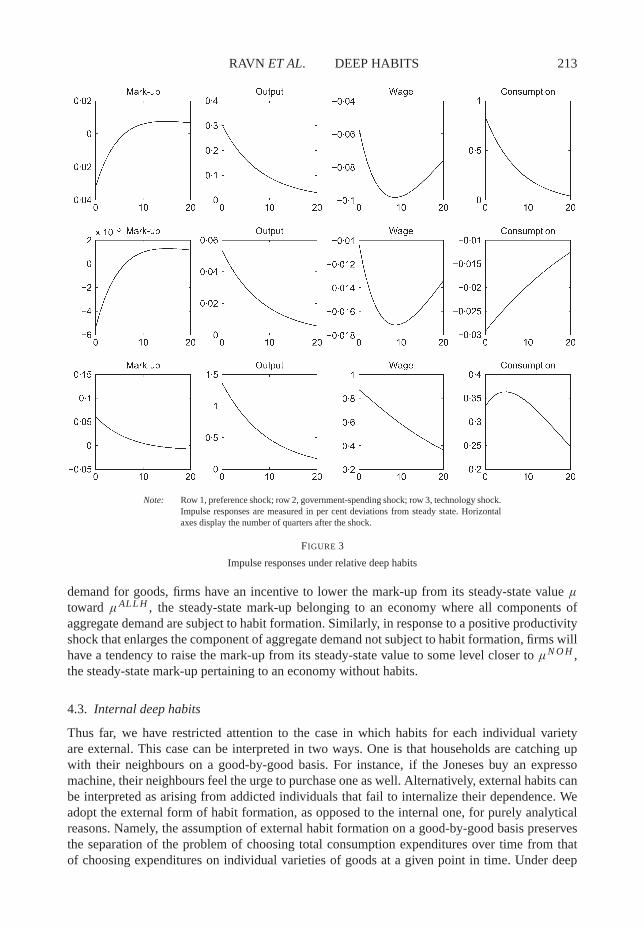
Figure 3 displays the dynamic response of the mark-up and other macroeconomic variablesof interest to positive preference, government-spending, and technology shocks. The behaviour ofmark-ups shown in the figure is dominated by changes in the composition of aggregate demand.To understand the effects of changes in the composition of demand on the equilibrium mark-up, it is of use to determine the steady-state value of the mark-up in the fully fledged relativehabit model, denoted µ, and in two variants thereof: namely, the steady-state mark-up in theabsence of deep habits (θ = θ g = 0), denoted by µN O H ; and the steady-state mark-up in a modelwhere investment spending is subject to habit formation, that is, the steady-state mark-up in aneconomy, where all components of aggregate demand are subject to habit formation, denoted byµALL H . It can be shown that µALL H < µ < µN O H (see Ravn et al., 2004b). Now, because boththe preference shock and the government-spending shock amplify the importance of the habitual



FIGURE 3

Impulse responses under relative deep habits

demand for goods, firms have an incentive to lower the mark-up from its steady-state value µtoward µALL H , the steady-state mark-up belonging to an economy where all components ofaggregate demand are subject to habit formation. Similarly, in response to a positive productivityshock that enlarges the component of aggregate demand not subject to habit formation, firms willhave a tendency to raise the mark-up from its steady-state value to some level closer to µN O H ,the steady-state mark-up pertaining to an economy without habits.

4.3. Internal deep habits

Thus far, we have restricted attention to the case in which habits for each individual varietyare external. This case can be interpreted in two ways. One is that households are catching upwith their neighbours on a good-by-good basis. For instance, if the Joneses buy an expressomachine, their neighbours feel the urge to purchase one as well. Alternatively, external habits canbe interpreted as arising from addicted individuals that fail to internalize their dependence. Weadopt the external form of habit formation, as opposed to the internal one, for purely analyticalreasons. Namely, the assumption of external habit formation on a good-by-good basis preservesthe separation of the problem of choosing total consumption expenditures over time from thatof choosing expenditures on individual varieties of goods at a given point in time. Under deep


internal habits, such separation is broken, and the consumer problem becomes more complex.Here, we explicitly consider the case of internal deep habits. In the Appendix, we show thatunder internal deep habits the aggregate demand for good i in the simple production economywithout capital of Section 2 takes the form

cit =[ ∞∑

k=0

θk Etrt,t+k pit+k

]−η

Xt + θcit−1,

where Xt is a measure of aggregate demand.This demand function shares key characteristics with that arising in the case of external

deep habits (equation (7)). Namely, the demand for each good variety is composed of two terms:a habitual term, θcit−1, that is completely price inelastic; and a price-elastic term,

[∑∞k=0

θk Etrt,t+k pit+k]−η

Xt , that is increasing in some measure of aggregate activity, Xt . All otherthings equal, if aggregate demand increases (Xt goes up), the relative importance of the price-elastic term rises and the elasticity of demand increases. This suggests a procyclical price elas-ticity as in the case of external deep habits.

However, a fundamental difference between external and internal deep habits is that underinternal deep habits, current demand for a particular variety depends not only on its currentrelative price but also on all future expected relative prices. This difference dramatically changesthe nature of the firm’s problem. In particular, under internal deep habits the firm’s problem isno longer time consistent, as in each period the monopolist has the incentive to renege fromprice promises made in the past that were optimal (profit maximizing) at the time they weremade. A full analysis of the optimal pricing behaviour under alternative economic environments(e.g. commitment or discretion in its many different forms such as Markov-perfect equilibria, orreputational equilibria) is beyond the scope of this paper and is left for future research.

4.4. Deep habits and sticky prices

Over the past decade, focus in macroeconomic research has shifted from the real-business-cycleparadigm to models in which nominal frictions are at centre stage, namely to the new Keynesiansynthesis. The key elements of the new Keynesian model are sticky product prices and monopolypower at the level of intermediate-goods-producing firms.

As in the deep-habit model, in the sticky-price model, mark-ups of prices over marginalcosts are positive and time varying. However, the mark-up dynamics implied by these two for-mulations are quite different. Indeed, Schmitt-Grohé and Uribe (2004) study a calibrated modelwith sticky prices à la Calvo–Yun and superficial habits, among several other real and nominalrigidities. Figures 1 and 2 of that paper display the response of the economy to productivity andgovernment-spending shocks, respectively, under the assumption that monetary policy takes theform of a simple Taylor rule. A number of features of these impulse responses serve as a guide toempirically distinguish between a sticky-price model with superficial habits and a flexible-pricemodel with deep habits. In response to a positive productivity shock the deep-habit model pre-dicts a decline in mark-ups, whereas the sticky-price model predicts an increase in mark-ups.3

Further, in response to a positive government-spending shock, consumption and real wages fall inthe sticky-price model, whereas in the deep-habit model both variables increase. Like the deep-habit model, the sticky-price model predicts a decline in mark-ups in response to an increase inpublic spending. However, the movements in mark-ups implied by the sticky-price model arequantitatively negligible (of the order of 0·01% in response to a 1% increase in public spending).

3. For the intuition behind this prediction of the sticky-price model see Schmitt-Grohé and Uribe (2004).


Doing justice to a comparison of the predictions of the deep-habit and sticky-price models liesoutside the scope of the present study.

A natural question that emerges from the above comparison is whether incorporating deephabits into the sticky-price model could improve the behaviour of mark-ups implied by thismodel. In Ravn, Schmitt-Grohé and Uribe (2004e), we study the case of sticky prices and deephabits. When deep habits are combined with sticky prices, the linearized Phillips curve becomes

πt = βEt πt+1 +κmct + θ

[κβ

1−βθmct −κ

µ−1

µβ[Et νt+1 + Et rt,t+1]

−κµ−1

µ

1

1− θ(yt − yt−1)

],

where a hat over a variable denotes per cent deviations from steady state, κ is a positive constant,and mct denotes marginal costs. Marginal costs are just the inverse of the mark-up, or µt =1/mct . All other variables and parameters are as defined earlier in the paper. First, note that inthe absence of deep habits, that is, when θ = 0, the Phillips curve is the same as in the standardneo-Keynesian model. We note that for a given inflation path, the mark-up in the sticky-pricemodel with deep habits differs from that in a sticky-price model without deep habit as follows:(1) all else constant, an increase in current output, yt > 0, reduces the mark-up and (2) all elseconstant, an increase in the future value of sales, νt+1 > 0, or a reduction in the discount rate,rt,t+1 > 0, reduces the mark-up. When monetary policy takes the form of a simple Taylor rule,then inflation falls in the sticky-price model without deep habits in response to a positive techno-logy shock. The above equation shows that as long as the current decline in inflation is largerthan the expected future inflation decline, marginal costs must fall, which is, mark-ups must rise.However, in the presence of deep habits, it is, in principle, possible that mark-ups fall instead,because output increases and the present value of future sales, Etrt,t+1νt+1, may increase. Sothere is the possibility that adding deep habits to a sticky-price model will result in the predictionthat mark-ups fall in response to a positive technology shock.

Another noteworthy feature of the Phillips curve in the sticky-price model with deep habitsis that it features lagged values of output. This is interesting because the inflation dynamics pre-dicted by the model may display more inertia. Standard sticky-price models have been criticizedheavily for their inability to predict the observed inertial behaviour of inflation.

5. CONCLUSION

In modern macroeconomics, it is commonplace to assume that households have preferences overa large number of differentiated goods. This assumption is made, for instance, in models withimperfectly competitive product markets. At the same time, there appears to be some consensusthat the assumption of habit formation is of great use in accounting for key business-cycle regu-larities, in particular, consumption and asset-price dynamics. An obvious question that emergesin modelling economies with habit formation and a large variety of goods available for consump-tion is at what level habits are formed. That is, are habits created at the level of each individualconsumption good or at the level of a consumption aggregate. The existing literature has focusedexclusively on the latter modelling strategy. This paper is motivated by our reading of the avail-able empirical literature on consumption behaviour suggesting that the former alternative is atleast equally compelling.

A central finding of our investigation is that the level at which habit formation is assumedto occur is of great macroeconomic consequence. When habits are formed at the level of eachindividual variety of consumption goods, the demand function faced by a firm depends not onlyon the relative price of the good and aggregate income—as in the standard case—but also on


past sales of the particular good in question. This characteristic of the demand function alters theoptimal pricing behaviour of the firm, for today’s prices are set taking into account that they willaffect not just today’s sales but also future sales through their effect on future demand. In thisway, the assumption of deep habits results in a theory of time-varying mark-ups. The deep-habitmodel developed in this paper provides microfoundations for other models in which past salesaffect current demand conditions at the level of each individual good, such as customer-marketand switching-cost models. General equilibrium versions of these models have been criticizedfor having the counterfactual implication that mark-ups are procyclical. To our knowledge, allexisting general equilibrium treatments of customer-market/switching-cost models use ad hocspecifications of the demand function faced by individual firms. In this paper, we show thatonce the demand faced by firms is derived from the behaviour of optimizing households, theresulting equilibrium comovement between mark-ups and aggregate activity can be in line withthe empirical evidence.

Most existing theories of countercyclical mark-ups face a trade-off between the elasticityof the mark-up with respect to aggregate demand and the level of the mark-up. Typically, whenthe average mark-up is restricted to empirically realistic levels, available theories predict toolow an elasticity of the mark-up to explain the cyclical behaviour of wages and consumption inresponse to demand shocks. An attractive feature of the additive version of the deep-habit modeldeveloped in this paper is that it overcomes this trade-off. That is, our theory can predict highmark-up elasticities without requiring empirically unrealistic levels of average mark-ups. Thisproperty suggests that the additive specification of deep habits offers the most fertile ground forfurther investigation.

For analytical convenience, in most of our analysis, habit formation is treated as external. Inthe existing related literature, however, the assumption of internal habit formation is prominent.Moreover, there is vast empirical support for the hypothesis of rational addictive behaviour at thelevel of individual consumption goods. We have studied the case of internal habit formation inSection 4.3. There, we have shown that the assumption of internal good-specific habit formationrenders the pricing behaviour of firms time inconsistent. However, because of the scope of thispaper, our analysis falls short of fully characterizing equilibrium dynamics under internal deep-habit formation. We believe that pursuing this avenue is, perhaps, the most relevant next step inthis research programme.

APPENDIX: INTERNAL DEEP HABITS

When good-specific habits are assumed to be internal, household j’s problem is to maximize the utility function (3)subject to the aggregation technology

x jt =

⎡⎢⎣

1∫0

(c ji t − θc j

i t−1)1−1/ηdi

⎤⎥⎦

1/(1−1/η)

,

the budget constraint1∫

0

pit cji t di + Etrt,t+1d j

t+1 = d jt +wt h

jt +�

jt ,

and some borrowing limit to avoid Ponzi schemes. The first-order conditions associated with this problem are

Ux (x jt ,h j

t )∂x j

t

∂c ji t

+βEtUx (x jt+1,h j

t+1)∂x j

t+1

∂c ji t

= λjt pi t ,

−Uh(x jt ,h j

t ) = λjt wt ,


andλ

jt rt,t+1 = βλ

jt+1.

Noting that ∂x jt+1/∂c j

i t = −θ∂x jt+1/∂c j

i t+1, we can write the first of the above optimality conditions as

z ji t = λ

jt pi t +βθ Et z

ji t+1,

wherez ji t = Ux (x j

t ,h jt )[x j

t ]1/η(c ji t − θc j

i t−1)−1/η.

Integrating the first of these expressions forward and under the assumption that z ji t is stationary (which is the case in the

class of equilibria we restrict attention to in this paper), we have

z ji t =

∞∑k=0

(βθ)k Etλjt+k pit+k .

Combining the last two expressions we obtain

c ji t =

⎡⎣ ∞∑

k=0

(βθ)k Etλjt+k pit+k

⎤⎦

−η

Ux (x jt ,h j

t )ηx jt + θc j

i t−1.

Recalling that λjt rt,t+1 = βλ

jt+1, we can write the above expression as

c ji t =

⎡⎣ ∞∑

k=0

θk Et rt,t+k pit+k

⎤⎦

−η [Ux (x j

t ,h jt )

λjt

]η

x jt + θc j

i t−1.

Integrating across households we obtain the following aggregate demand function for good i in period t

ci t =⎡⎣ ∞∑

k=0

θk Et rt,t+k pit+k

⎤⎦

−η

Xt + θcit−1,

where Xt ≡ ∫ 10

[Ux (x j

t ,h jt )

λjt

]η

x jt d j is a measure of aggregate demand.

Acknowledgements. We thank for comments Pierpaolo Benigno, Julio Rotemberg, Mike Woodford, and seminarparticipants at Columbia University, Duke University, the University of North Carolina, the University of Southamp-ton, the 2004 ESSIM meeting (Tarragona), the IIES (Stockholm), the European University Institute (Florence), theFederal Reserve Banks of Chicago, Cleveland, and Atlanta, Emory University, and the 2004 Australian Conferenceof Economists. Ravn gratefully acknowledges financial support from the RTN project “Macroeconomic Policy Designfor Monetary Unions”, funded by the European Commission (contract number HPRN-CT-2002-00237).

REFERENCESABEL, A. B. (1990), “Asset Prices under Habit Formation and Catching Up with the Joneses”, The American Economic

Review Papers and Proceedings, 80, 38–42.BLANCHARD, O. and PEROTTI, R. (2002), “An Empirical Characterization of the Dynamic Effects of Changes in

Government Spending and Taxes on Output”, Quarterly Journal of Economics, 117, 1329–1368.CHINTAGUNTA, P., KYRIAZIDOU, E. and PERKTOLD, J. (2001), “Panel Data Analysis of Household Brand

Choices”, Journal of Econometrics, 103, 111–153.COOLEY, T. F. and PRESCOTT, E. C. (1995), “Economic Growth and Busines Cycles”, in T. F. Cooley (ed.) Frontiers

of Business Cycle Research (Princeton, NJ: Princeton University Press) 1–38.FATÁS, A. and MIHOV, I. (2001), “The Effects of Fiscal Policy on Consumption and Employment” (Manuscript, Insead).GALÍ, J., LÓPEZ-SALIDO, D. and VALLÉS, J. (2003), “Understanding the Effects of Government Spending on

Consumption” (Manuscript, CREI).GALÍ, J. and RABANAL, P. (2004), “Technology Shocks and Aggregate Fluctuations: How Well Does the RBC Model

Fit Postwar U.S. Data?” (Manuscript, CREI).HOUTHAKKER, H. S. and TAYLOR, L. D. (1970) Consumer Demand in the United States: Analyses and Projections

(Cambridge: Harvard University Press).KLEMPERER, P. (1995), “Competition when Consumers have Switching Costs: An Overview with Applications to

Industrial Organization, Macroeconomics, and International Trade”, Review of Economic Studies, 62, 515–539.


PHELPS, E. S. and WINTER, S. G. (1970), “Optimal Price Policy under Atomistic Competition”, in E. S. Phelps (ed.)Microeconomic Foundations of Employment and Inflation Theory (New York: W. W. Norton) 309–337.

PRESCOTT, E. C. (1986), “Theory Ahead of Business Cycle Measurement”, Federal Reserve Bank of MinneapolisQuarterly Review, 10, 9–22.

RAVN, M., SCHMITT-GROHÉ, S. and URIBE, M. (2004a), “Deep Habits: Technical Notes” (Manuscript, DukeUniversity).

RAVN, M., SCHMITT-GROHÉ, S. and URIBE, M. (2004b), “Relative Deep Habits” (Manuscript, Duke University).RAVN, M., SCHMITT-GROHÉ, S. and URIBE, M. (2004c), “The Macroeconomics of Subsistence Points” (Manuscript,

Duke University).RAVN, M., SCHMITT-GROHÉ, S. and URIBE, M. (2004d), “Deep Habits” (NBER Working Paper No. 10261).RAVN, M., SCHMITT-GROHÉ, S. and URIBE, M. (2004e), “Deep Habits and Sticky Prices: A Technical Note”

(Manuscript, Duke University).ROTEMBERG, J. J. and SALONER, G. (1986), “A Supergame-Theoretic Model of Price Wars During Booms”,

American Economic Review, 76, 390–407.ROTEMBERG, J. J. and WOODFORD, M. (1991), “Markups and the Business Cycle”, in O. J. Blanchard and S. Fischer

(eds.) NBER Macroeconomics Annual (Cambridge, MA: MIT Press) 63–129.ROTEMBERG, J. J. and WOODFORD, M. (1992), “Oligopolistic Pricing and the Effects of Aggregate Demand on

Economic Activity”, Journal of Political Economy, 100, 1153–1207.ROTEMBERG, J. J. and WOODFORD, M. (1995), “Dynamic General Equilibrium Models with Imperfectly Competitive

Product Markets”, in T. F. Cooley (ed.) Frontiers of Business Cycle Research (Princeton, NJ: Princeton UniversityPress) 243–293.

ROTEMBERG, J. J. and WOODFORD, M. (1999), “The Cyclical Behavior of Prices and Costs”, in J. B. Taylor andM. D. Woodford (eds.) Handbook of Macroeconomics (Amsterdam: North-Holland) 1051–1135.

SCHMITT-GROHÉ, S. and URIBE, M. (2004), “Optimal Operational Monetary Policy in the Christiano–Eichenbaum–Evans Model of the U.S. Business Cycle” (NBER Working Paper No. 10724).

deep habits - columbia.edumu2166/deep_habits/res_version.pdf · ravn et al. deep habits 197 because...

Documents