IN DEGREE PROJECT COMPUTER SCIENCE AND ENGINEERING,SECOND CYCLE, 30 CREDITS

, STOCKHOLM SWEDEN 2021

Deep Learning for Chromosome Segmentation with Uncertainty Estimation

ARVID NORSTRÖM

KTH ROYAL INSTITUTE OF TECHNOLOGYSCHOOL OF ELECTRICAL ENGINEERING AND COMPUTER SCIENCE

Deep Learning forChromosome Segmentationwith Uncertainty Estimation

ARVID NORSTRÖM

Master’s Programme, Machine Learning, 120 creditsDate: June 28, 2021

Supervisor: Mårten BjörkmanExaminer: Danica Kragíc Jensfelt

School of Electrical Engineering and Computer ScienceHost company: Arkus AISwedish title: Djupinlärning för Kromosomsegmentering medOsäkerhetsestimation

© 2021 Arvid Norström

| i

AbstractKaryotyping, the process of pairing and ordering chromosomes, is an importanttool for cytogenetic analysis to detect chromosome abnormalities. A trainedspecialist analyses the resulting image of the karyotyping, known as a karyogram,paying attention to the size, shape, and number of the chromosomes. However,manual inspection is a time-consuming task and necessitates domain expertise.Thus, there is a great interest in automating this process to allow moreindividuals access to clinical genetics. One important piece of this puzzleis segmentation, whereby the individual chromosomes are delineated andseparated from the background. Nevertheless, this becomes difficult whenthere are overlapping chromosomes in the original micrograph. Furthermore,most employed deep learning models are unable to alert the user whenthe segmentation is likely to fail. This thesis aims to bring clarity to theaforementioned issues. Firstly, an augmented dataset consisting of overlappingchromosomes is created, which is then used to train a convolutional neuralnetwork inspired by the original U-Net implementation, but with dropoutlayers, batch normalization and padding to ensure equal sizes of input andoutput. Our proposed model achieves a validation accuracy of 97.4 %.Different uncertainty metrics were then compared in terms of predictivecapacity of the segmentation accuracy, both qualitatively from the uncertaintymaps and quantitatively by computing the correlation. The results showedthat the uncertainty obtained with Monte Carlo Dropout and Test TimeAugmentation, bothmeasured using entropy, were themost promising approachesto predict the accuracy. The uncertainty maps were used as training dataon a regression problem with a ResNet network as our model to predictsegmentation accuracy, where we could not demonstrate any significantbenefit of the uncertainty estimations compared to the benchmark models.

ii |

| iii

SammanfattningKaryotyping, en process där kromosomer delas in och sorteras efter par, är ettviktigt verktyg för cytogenetisk analys för att detektera kromosomavvikelser.En tränad specialist analyserar den resulterande bilden från karyotyping,känt som ett karyogram, och tar hänsyn till storleken, formen och antaletkromosomer.Manuell inspektion av det här slaget är emellertid en tidskrävandeuppgift och kräver domänexpertis. Det finns därför ett stort intresse i attautomatisera den här processesen för att ge fler individer tillgång till kliniskgenetik. En viktig del i det här pusslet är segmentering, där individuellachromosomer är utskurna och seperararde från bakgrunden. Det här blir docksvårt när det finns överlappande kromosomer i originalmikrografen. Dessutomsaknar de flesta djupinlärningsmetoder möjlighet att varna användaren närsegmententeringen troligtvis misslyckas. Denna uppsats ämnar bringa klarhettill de föregående problemen. Först av allt skapas ett utökat dataset beståendeav överlappande kromosomer, vilket sen används för att träna ett convolutionalneural network inspirerat av den ursprungliga U-Net implementationen, menmed dropoutlager, batch normalization och padding för att säkerställa att in-och utdata är av samma storlek. Vår föreslagnamodell uppnår en validitetsprecisionpå 97.4 %. Olika osäkerhetsestimeringsmetriker jämfördes sedan efter derasprediktiva kapacitet att mäta segmenteringsprecisionen, både kvalitativt frånosäkerhetsbilderna och kvantitativt genom att beräkna korrelationen. Resultatenvisade att osäkerheten uppmätt genom Monte Carlo Dropout och Test TimeAugmentation, där entropi användes som mätinstrument, var de mest lovandeangreppssätten för att förutsäga precisionen. Osäkerhetsbilderna användessom träningsdata för ett regressionsproblem med ett ResNet-nätverk somvår modell för att förutsäga segmenteringsprecisionen, där vi inte kundedemonstrera någon signifikant fördel med osäkerhetsestimeringarna jämförtmed benchmarkmodellerna.

iv |

Acknowledgments | v

AcknowledgmentsI would like to express my most sincere gratitude to Vladimir Li, who acted asmy supervisor at Arkus AI, for his continuous support and invaluable feedbackduring the course of the project. Vladimir provided not only his technicalexpertise but also set out a clear path for me to follow. I would also like to thankmy supervisor at KTH, Mårten Björkman, for his suggestions and interest inmy work. Last but not least, I deeply appreciate the opportunity given to meby the founder of Arkus AI, Ying Chen, to take a part in the cause to makemedical genetics available for everyone.

Thank you,Arvid Norström

vi | CONTENTS

Contents

1 Introduction 11.1 Background . . . . . . . . . . . . . . . . . . . . . . . . . . . 11.2 Problem . . . . . . . . . . . . . . . . . . . . . . . . . . . . . 21.3 Goals . . . . . . . . . . . . . . . . . . . . . . . . . . . . . . 21.4 Ethics and Societal Impact . . . . . . . . . . . . . . . . . . . 21.5 Research Methodology . . . . . . . . . . . . . . . . . . . . . 31.6 Delimitations . . . . . . . . . . . . . . . . . . . . . . . . . . 31.7 Structure of the thesis . . . . . . . . . . . . . . . . . . . . . . 3

2 Background 52.1 Karyotyping . . . . . . . . . . . . . . . . . . . . . . . . . . . 52.2 Semantic segmentation . . . . . . . . . . . . . . . . . . . . . 62.3 Networks . . . . . . . . . . . . . . . . . . . . . . . . . . . . 7

2.3.1 Convolutional Neural Network . . . . . . . . . . . . . 72.3.2 U-Net . . . . . . . . . . . . . . . . . . . . . . . . . . 72.3.3 ResNet . . . . . . . . . . . . . . . . . . . . . . . . . 8

2.4 Uncertainty Estimation . . . . . . . . . . . . . . . . . . . . . 92.4.1 Measuring Aleatoric Uncertainty . . . . . . . . . . . 92.4.2 Measuring Epistemic Uncertainty . . . . . . . . . . . 112.4.3 Combining Aleatoric and Epistemic Uncertainty . . . 11

2.5 Data Augmentation . . . . . . . . . . . . . . . . . . . . . . . 122.6 Related Work . . . . . . . . . . . . . . . . . . . . . . . . . . 13

3 Methods 153.1 Networks and Algorithms . . . . . . . . . . . . . . . . . . . . 15

3.1.1 U-Net . . . . . . . . . . . . . . . . . . . . . . . . . . 153.1.2 ResNet . . . . . . . . . . . . . . . . . . . . . . . . . 163.1.3 Monte Carlo Dropout . . . . . . . . . . . . . . . . . . 163.1.4 Learning Loss Attenuation . . . . . . . . . . . . . . . 17

Contents | vii

3.1.5 Test time Augmentation . . . . . . . . . . . . . . . . 173.2 Data . . . . . . . . . . . . . . . . . . . . . . . . . . . . . . . 183.3 Implementation Details . . . . . . . . . . . . . . . . . . . . . 183.4 Metrics for Accuracy and Uncertainty . . . . . . . . . . . . . 19

3.4.1 Jaccard Index . . . . . . . . . . . . . . . . . . . . . . 193.4.2 Variance and Entropy . . . . . . . . . . . . . . . . . . 193.4.3 Pearson Correlation Coefficient . . . . . . . . . . . . 20

4 Results 214.1 Segmentation accuracy . . . . . . . . . . . . . . . . . . . . . 214.2 Uncertainty Estimations . . . . . . . . . . . . . . . . . . . . . 21

4.2.1 Monte Carlo Dropout . . . . . . . . . . . . . . . . . . 224.2.2 Test Time Augmentation . . . . . . . . . . . . . . . . 224.2.3 Heteroscedastic Variance . . . . . . . . . . . . . . . . 244.2.4 Pearson Correlation Coefficients . . . . . . . . . . . . 25

4.3 Predicting Accuracy . . . . . . . . . . . . . . . . . . . . . . . 26

5 Discussion 33

6 Conclusions and Future work 356.1 Conclusions . . . . . . . . . . . . . . . . . . . . . . . . . . . 356.2 Future Work . . . . . . . . . . . . . . . . . . . . . . . . . . . 35

References 37

viii | Contents

LIST OF FIGURES | ix

List of Figures

2.1 A typical G-banding karyogram. . . . . . . . . . . . . . . . . 62.2 Graphical representation of U-Net as introduced in the original

paper [1]. . . . . . . . . . . . . . . . . . . . . . . . . . . . . 82.3 The building block in the residual network [2]. . . . . . . . . . 82.4 From left to right: input image, ground truth, segmentation,

aleatoric and epistemic uncertainty [3] . . . . . . . . . . . . 12

4.1 Training and validations results in terms of loss and segmentationduring the training phase of the U-Net. . . . . . . . . . . . . . 22

4.2 Distribution over the segmentation accuracies on the validationset. . . . . . . . . . . . . . . . . . . . . . . . . . . . . . . . . 23

4.3 Example segmentation of a sample from the validation set. . . 234.4 Epistemic uncertainty acquired by performing MC dropout

with T = 20 samples. . . . . . . . . . . . . . . . . . . . . . . 244.5 Aleatoric uncertainty acquired by performing TTA. . . . . . . 244.6 Heteroscedastic variance (HV) given by the predicted variance

by the network. The left plot shows the predicted pixel-wisevariance whereas the right plot shows the inverted predictedvariance. . . . . . . . . . . . . . . . . . . . . . . . . . . . . 25

4.7 PCC for the different uncertainty metrics. . . . . . . . . . . . 264.8 Aleatoric uncertainty acquired by performing TTA on the

noised sample. . . . . . . . . . . . . . . . . . . . . . . . . . . 274.9 Epistemic uncertainty acquired by performing MCDO with

T = 20 MC samples. . . . . . . . . . . . . . . . . . . . . . . 284.10 Example of a noised sample, together with the target and

output segmentation. . . . . . . . . . . . . . . . . . . . . . . 294.11 Distribution over the segmentation accuracies on the noised

samples. . . . . . . . . . . . . . . . . . . . . . . . . . . . . . 29

x | LIST OF FIGURES

4.12 Heteroscedastic aleatoric uncertainty given by the predictedvariance by the network. . . . . . . . . . . . . . . . . . . . . 30

4.13 Heteroscedastic aleatoric uncertainty given by the predictedvariance by the network. . . . . . . . . . . . . . . . . . . . . 31

LIST OF TABLES | xi

List of Tables

3.1 Design of the U-Net. . . . . . . . . . . . . . . . . . . . . . . 16

4.1 Mean relative validation error after 15 epochs together withthe corresponding standard deviation for the five differentResNet models. . . . . . . . . . . . . . . . . . . . . . . . . . 28

xii | LIST OF TABLES

Introduction | 1

Chapter 1

Introduction

1.1 BackgroundA healthy human cell has 46 chromosomes, where the first 22 pairs areknown as autosomes and the 23rd pair are the sex chromosomes X and Y.There are two ways cells divide and reproduce: mitosis and meiosis, andchromosomal abnormalities can occur before, during and after these stages.For example, Klinefelter syndrome is a trisomy disorder characterized by anextra X chromosome in males. Karyotyping is a procedure used in medicalgenetics to identify and order pairs of chromosomes found in a cell, which canthen be used as a diagnostical tool in clinical genetics. Manual karyotyping is ahighly time-consuming task and requires domain expertise by a cytogeneticist.It is thus of interest to develop reliable and accurate methods to automatize theprocess. Automatic karyotyping is typically divided into four stages which areperformed in the following order: image enhancement and coarse refinement(for example, removing the nucleus if present), chromosome segmentation,feature extraction and lastly classification. This thesis is primarily focused onchromosome segmentation.

Semantic segmentation is a pixel-level prediction where each pixel in theimage is assigned a label. With the advancement of deep learning, therenow exists numerous tried and tested architectures and algorithms suitablefor high-performance segmentation. However, most deep learning modelsare unable to represent the uncertainty in their predictions. Measuring andunderstanding the uncertainty is especially important in safety-critical systemssuch as medical applications. We therefore aim to present a model capable ofoutputting accurate chromosome segmentations while providing uncertaintyestimations of the segmentation.

2 | Introduction

1.2 ProblemThe first part of this project is concerned with developing a deep learningmodel, namelyU-Net, to segment overlapping chromosomes from a syntheticallyaugmented dataset. In the second part, we provide different uncertaintyestimations of these segmentations. Lastly, in the third part, we investigatethe potential of using the uncertainty estimations to predict the segmentationaccuracy using a Resnet on a dataset consisting of both clean samples andnoised samples. The problem statement can be formulated as follows:

Is there a quantitative benefit of harnessing the uncertainty estimations inthe context of predicting the segmentation accuracy?

1.3 GoalsThe main objective of the project is to use deep learning methods to utilizeuncertainty estimation to improve the relative prediction of the segmentationaccuracy. This is an important part in the automatic karyotyping process, asto understand when the segmentation task is likely to fail.

1.4 Ethics and Societal ImpactGreat care has to be taken to ensure security and anonymity of the patient data.We thus elected to remove any details that could be linked to an identity duringthe gathering and categorization of the data. The company provides a secureplatform to prevent external access to the trained models.

There is great potential in incorporating uncertainty into our deep learningmodels to know whether the results are to be trusted or not. Indeed, reliableanalytical tools are of immense importance in safety-critical applications suchas in the field of medical genetics, where the consequences of misleadingresults may be particularly grave. This work is only a small part in the workof automatic karyotyping, which in the larger picture has the potential togreatly increase the efficiency of screening for genetic diseases. Additionally,redistributing resources by automating diagnostical allows allows the medicalprofessionals such as cytogeneticists to perform tasks that typically requirehuman intervention.

Introduction | 3

1.5 Research MethodologyThe initial phase of the project aims to survey the field to gain an insightinto promising methods, both for chromosome segmentation and uncertaintyestimation approaches for computer vision tasks. The selected methods basedon the findings from the literature study were then evaluated using statisticaltools such as Pearson correlation coefficient (PCC), which is explained ingreater detail in section 3.4.3, to bring quantitive clarity to the researchquestion.

1.6 DelimitationsThere is no explicit aim to improve upon existingmodels regarding chromosomesegmentation. Rather, we are more interested in investigating the usefulnessof different metrics of uncertainty on the segmentations. Furthermore, it isoutside of the scope of this degree project to perform a comprehensive studyof such metrics and we thus prioritized broadness rather than depth in ourselection. We also limit the dataset to one that is artifically generated, due tothe lack of high quality existing datasets suitable for our particular needs.

1.7 Structure of the thesisIn chapter two, we introduce the relevant background to understand the subjectmatter and briefly recaps previous work. Next, chapter three introduces theneural networks employed in the study, the pre-processing and manipulationof the data, implementation details of the neural networks and the metrics usedto quantitatively describe the results. The results from the experiments aredescribed in chapter four. We then discuss the results in chapter 5 and lastlyconclude our work in chapter 6, while outlining potential avenues for futurework.

4 | Introduction

Background | 5

Chapter 2

Background

This chapter describes the background of the degree project. To begin with, weintroduce the topic of karyotyping in Section 2.1. Essential to the topic at handis semantic segmention, which is briefly described in Section 2.2. Thereafter,we provide an introduction to convolutional neural networks in Section 2.3,followed by characterizing the particular CNNs U-Net and ResNet, which willbe used for segmentation ad predicting the segmentation accuracy respectively.The different approaches to measuring the uncertainty are presented in Section2.4. The technique of data augmentation, which is used extensively in thisproject, is introduced in Section 2.5. Lastly, we give an overview of someprevious work on the topic of segmenting chromosomes in Section 2.6.

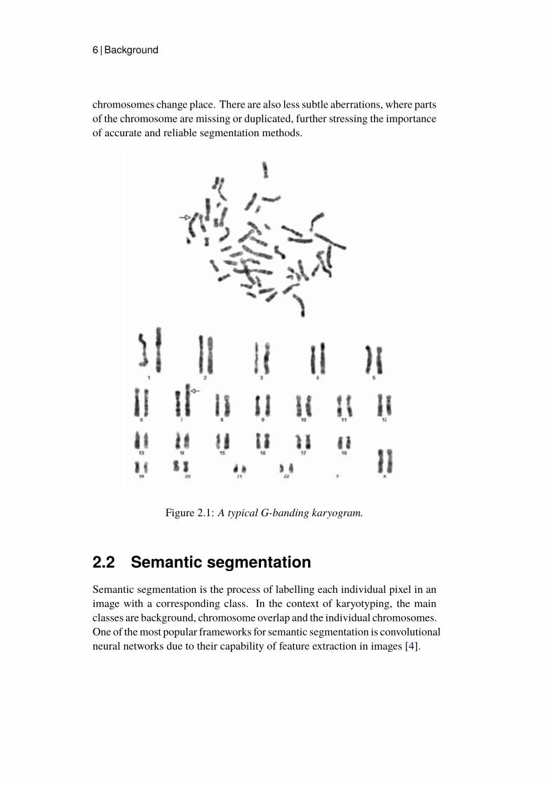
2.1 KaryotypingKaryotyping is the process of pairing and ordering the chromosomes, given amicroscopic image of the chromosomes in a cell. A common technique usedin cytogenetics, the study of chromosomes, is to employ the technique knownas Giemsa stain on the condensed chromosomes in metaphase to producevisible bands on the chromosomes, facilitating the process of producing visiblekaryotpes. The resulting karyogram, as the one presented in Figure 2.1, isthen examined by the number and structure of the chromosomes in order todetect chromosomal abnormalities. A numerical deviation from the typical46 chromosomes in a healthy cell is regarded as a numerical abnormality.The condition is known as monosomy when an individual is missing oneof the chromosomes from a pair, and trisomy when the individual has threechromosomes instead of a pair. The cytogeneticist also look for structuralabnormalities, for example translocations, where segments from different

6 | Background

chromosomes change place. There are also less subtle aberrations, where partsof the chromosome are missing or duplicated, further stressing the importanceof accurate and reliable segmentation methods.

Figure 2.1: A typical G-banding karyogram.

2.2 Semantic segmentationSemantic segmentation is the process of labelling each individual pixel in animage with a corresponding class. In the context of karyotyping, the mainclasses are background, chromosome overlap and the individual chromosomes.One of themost popular frameworks for semantic segmentation is convolutionalneural networks due to their capability of feature extraction in images [4].

Background | 7

2.3 Networks

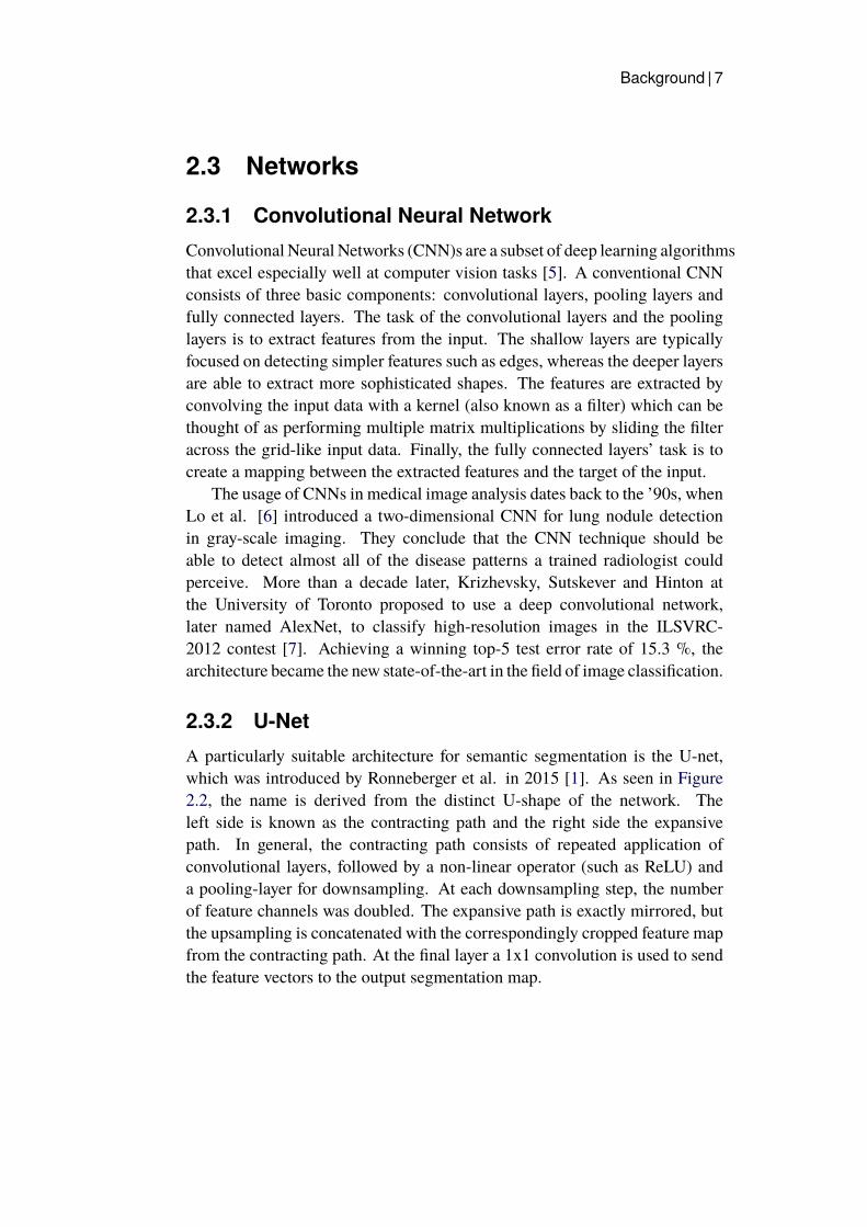
2.3.1 Convolutional Neural NetworkConvolutional Neural Networks (CNN)s are a subset of deep learning algorithmsthat excel especially well at computer vision tasks [5]. A conventional CNNconsists of three basic components: convolutional layers, pooling layers andfully connected layers. The task of the convolutional layers and the poolinglayers is to extract features from the input. The shallow layers are typicallyfocused on detecting simpler features such as edges, whereas the deeper layersare able to extract more sophisticated shapes. The features are extracted byconvolving the input data with a kernel (also known as a filter) which can bethought of as performing multiple matrix multiplications by sliding the filteracross the grid-like input data. Finally, the fully connected layers’ task is tocreate a mapping between the extracted features and the target of the input.

The usage of CNNs in medical image analysis dates back to the ’90s, whenLo et al. [6] introduced a two-dimensional CNN for lung nodule detectionin gray-scale imaging. They conclude that the CNN technique should beable to detect almost all of the disease patterns a trained radiologist couldperceive. More than a decade later, Krizhevsky, Sutskever and Hinton atthe University of Toronto proposed to use a deep convolutional network,later named AlexNet, to classify high-resolution images in the ILSVRC-2012 contest [7]. Achieving a winning top-5 test error rate of 15.3 %, thearchitecture became the new state-of-the-art in the field of image classification.

2.3.2 U-NetA particularly suitable architecture for semantic segmentation is the U-net,which was introduced by Ronneberger et al. in 2015 [1]. As seen in Figure2.2, the name is derived from the distinct U-shape of the network. Theleft side is known as the contracting path and the right side the expansivepath. In general, the contracting path consists of repeated application ofconvolutional layers, followed by a non-linear operator (such as ReLU) anda pooling-layer for downsampling. At each downsampling step, the numberof feature channels was doubled. The expansive path is exactly mirrored, butthe upsampling is concatenated with the correspondingly cropped feature mapfrom the contracting path. At the final layer a 1x1 convolution is used to sendthe feature vectors to the output segmentation map.

8 | Background

Figure 2.2: Graphical representation of U-Net as introduced in the originalpaper [1].

2.3.3 ResNetTo create a mapping between the output from the U-Net and the predictedsegmentation accuracy, a convolutional network with scalar output is needed.Taking inspiration from the field of image recognition, we suggest using aresidual neural network (ResNet) to this aim, which achieved state-of-the-artresults on the ILSVRC-2015 classification task [2]. A long standing problemof gradient based methods is that of vanishing gradient, which becomesincreasingly difficult to solve as the model grows deeper [8]. ResNet aimsto solve this by inserting shortcut connections, where the input and outputfrom a previous layer are stacked together as input to a subsequent layer. Thefundamental building block of this type of shortcut connection can be seen inFigure 2.3.

Figure 2.3: The building block in the residual network [2].

Background | 9

2.4 Uncertainty EstimationThis section will introduce the relevant uncertainty estimation (in someliterature known as uncertainty quantification) taxonomy. The topic of uncertaintyestimation is central to the thesis, as to inform the user of the end-productwhen the algorithm is not sufficiently certain of the output. There are twomain sources of uncertainty - aleatoric and epistemic. Aleatoric uncertaintyis due to an inherently stochastic dependency between the input and the output.Thus, this source of uncertainty cannot be "explained away" by incorporatingmore data in the training set. Aleatoric uncertainty can further be divided intohomoscedastic and heterscedastic uncertainty. Homoscedastic uncertainty isuniform over the input, whereas heteroscedastic uncertainty instead dependson the input. Epistemic uncertainty on the other hand captures our ignoranceabout the models that are most suitable to explain our data [9]. In fact,epistemic uncertainty encapsulates both model uncertainty and approximationuncertainty and can be reduced by adding more data. Most previous work hasfocused on either aleatoric or epistemic uncertainty, but there are approachesthat enable us to model both categories of uncertainty [3].

2.4.1 Measuring Aleatoric UncertaintyOne of the most common methods of modeling aleatoric uncertainty formedical image segmentation is known as test time augmentation (TTA).Usually, data augmentation is done during the training stage of the implementationin order to expand the training set with altered copies of samples fromthe training dataset. It is especially tangible for image data, where imagemanipulation techniques include rotations, zooms, crops, shifts, flips, noisingand so on. In TTA, these data augmentation procedures are applied to the testdataset.

Wang et al. [10] showed that TTA can be cast as a performing inferencewith hidden parameters by using entropy for uncertainty estimation. Morespecifically, denote the input image as X0 and let X = τβ(X0) + ε be theaugmented image, which will be used for inference at test time. τβ representsthe transformation operator with parameters β and ε is simply additive noise.Assume the τ is a reversible spatial transformation such that an inverse existsandX0 = τ−1β (X− ε). In the context of deep learning, we may let f(·) denotethe function representation by a neural network and θ the learnable parameters.Thus, Y = f(X, θ) is the prediction of a test image, which in segmentationtasks corresponds to discretized labels (usually obtained by argmax operation

10 | Background

in the final layer of the network). However,X is only one out of many possibleobservations of the latent imageX0 and so direct inferencemay lead to a biasedresult. Therefore, it is preferred to perform inference using X0 instead as:

Y = τβ(f(θ,X0)) = τβ(f(θ, τ−1β (X − ε))) (2.1)

The posterior distribution is then given by:

p(Y |X) = p(τβ(f(θ, τ−1β (X − ε)))) (2.2)

where β ∼ p(β) and ε ∼ p(ε) are sampled from known prior distributions.The final prediction for X is given by maximum likelihood estimation bytaking the argmax:

Y = arg maxy

p(y|X) ≈Mode(y) (2.3)

where Mode is the majority vote. The entropy of the posterior distribution isthen used to estimate the uncertainty:

H(Y |X) = −∫p(y|X) log(p(y|X))dy (2.4)

Since this integral is intractable for most distributions, we use Monte Carlosimulation to approximate it as:

H(Y i|X) ≈ −K∑k=1

pik log(pik) (2.5)

where Y i is the predicted label for the i:th pixel and pik is the frequency ofthe k:th unique value in a set of labels obtained during the Monte Carlo (MC)simulation. The authors ran experiments on MRI scans of fetal brains andconclude that "[...] TTA leads to higher segmentation accuracy than a single-prediction baseline and multiple predictions using test-time dropout" [10].More specifically, their dataset consisted of 2D and 3D magnetic resonanceimages (MRI) of fetal brains and brain tumors and the TTA was comparedboth in terms of accuracy and uncertainty estimation. The usefulness ofthe uncertainty estimation was compared to that of test time dropout (TTD),which is an epistemic measure. The benchmark for accuracy was a single-prediction that obtains the predictionwithout TTAor TTD. The transformationoperations used were flipping (along the horizontal and the vertical axis),

Background | 11

rotational, scaling and additive random noise. The segmentation accuracywas improved compared to the single-prediction baseline and the uncertaintyestimation with TTA helped to lower the number of overconfident incorrectpredictions in comparison to the uncertainty estimation of TTD.

Shanmugam et al. considered the performance of TTA on two widelyused datasets for image classification - ImageNet and Flowers102 [11]. Byflipping, cropping and scaling the input images, they found that TTA overallhad a positive effect on the accuracy of the classification, but that the gain wasinversely correlated with the accuracy of the model.

2.4.2 Measuring Epistemic UncertaintyOne of the most common approaches to model epistemic uncertainty in thefield of medical imaging is MC dropout. Dropout is probably familar tomost practitioners in applied machine learning as a technique to regularizedeep neural networks. In essence, a single model can be used to simulatean ensemble of different network architectures by randomly dropping outnodes during training [12]. MC dropout has been empirically proven tosignificantly improve the prediction of segmentation quality, as compared tonot incorporating uncertainty at all in the model, demonstrated for exampleby DeVries et al. [13]. In their implementation of U-net, dropout was appliedafter every convolutional layer, and then samples from segmentation networkwere drawn during test time to approximate MC integration. As in the TTAexample above, the entropy of the averaged probability was used as a measureof uncertainty.

2.4.3 Combining Aleatoric and Epistemic UncertaintyIn many cases, it might be reasonable to model both aleatoric and epistemicuncertainty. For example, it is difficult to know how each source of uncertaintyaffects the result in advance. It can therefore be advantageous to model both.Kendall and Gal [3] showed that it is possible to combine heteroscedasticaleatoric uncertainty and epistemic uncertainty in a quite simply way. Assumea neural network (NN) designed to perform segmentation is parametrized by θand some labelled dataset {yi, xi}Ni=1 with some input-dependent noise σ(xi).The noise parameter can be learned as a function of the data by including it in

12 | Background

the loss function:

LNN(θ) =1

N

N∑i=1

1

2σ(xi)2||yi − f(xi)||2 +

1

2log σ(xi)

2 (2.6)

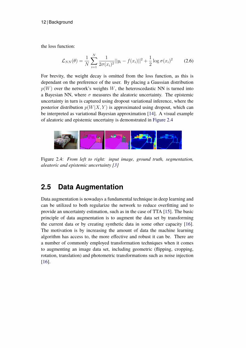
For brevity, the weight decay is omitted from the loss function, as this isdependant on the preference of the user. By placing a Gaussian distributionp(W ) over the network’s weights W , the heteroscedastic NN is turned intoa Bayesian NN, where σ measures the aleatoric uncertainty. The epistemicuncertainty in turn is captured using dropout variational inference, where theposterior distribution p(W |X, Y ) is approximated using dropout, which canbe interpreted as variational Bayesian approximation [14]. A visual exampleof aleatoric and epistemic uncertainy is demonstrated in Figure 2.4

Figure 2.4: From left to right: input image, ground truth, segmentation,aleatoric and epistemic uncertainty [3]

2.5 Data AugmentationData augmentation is nowadays a fundamental technique in deep learning andcan be utilized to both regularize the network to reduce overfitting and toprovide an uncertainty estimation, such as in the case of TTA [15]. The basicprinciple of data augmentation is to augment the data set by transformingthe current data or by creating synthetic data in some other capacity [16].The motivation is by increasing the amount of data the machine learningalgorithm has access to, the more effective and robust it can be. There area number of commonly employed transformation techniques when it comesto augmenting an image data set, including geometric (flipping, cropping,rotation, translation) and photometric transformations such as noise injection[16].

Background | 13

2.6 Related WorkThe U-Net architecture can be modified in a number of ways, for example byaddingmore layers as to help extract more complex features and thus hopefullyincrease segmentation accuracy. However, the increased model complexitymay lead to overfitting [17]. Recently a proposed modification of U-Net withadditional CNN layers mitigated the problem by implementing test TTA [18].TTA is similar to regular data augmentation that is typically done duringtraining, but is, as the name suggests, instead performed during test time. Inthis particular case, the authors applied horizontal and vertical image flippingduring test time. Comparing the performance on a publicly available dataset ofoverlapping chromosomes [19], they improved upon a similar implementationusing a modified U-Net but without TTA [20].

One team of researchers recently published a study, where they proposedan automatic chromosome extraction method based on a combination of U-Net and YOLOv3 [21]. You only look once, or YOLO, is a CNN used forobject detection and derives its name from the fact that it only requires a singleforward propagation pass to predict the bounding boxes [22]). The modelconsists of three steps: First, U-Net is used to remove the nuclei and otherinterferences in the background of the chromosome micro- graphs. Second,YOLOv3 is used to identify and predict bounding boxes for each chromosome.Finally, U-Net is used again to extract the chromosomes in a more precisemanner. By measuring the number of correctly extracted chromosomes on atest set, the authors claim to have achieved an accuracy of 99.3%, showingthat their method can reliably extract the single, overlapping and adhesivechromosomes from the raw G-band chromosome images. The authors alsoimplementedMask R-CNN [23] but with poor chromosome extraction results,citing the relatively low number of micrographs as a possible explanation ofthe unsatisfactory results.

PSPNet, or Pyramid Scene Parsing Network, is another model used forsemantic segmentation [24]. It is a fully convolutional network (FCN) justlike U-Net and is suitable for procesessing raw images without complexpre-processing. The PSPNet and U-Net were compared on chromosomesegmentation by Chen et al [25]. Furthermore, the authors introduce twodifferent ways of simulating overlapped chromosomes: one by summing thepixel values in the overlapped chromosome region and the other by randomlysampling the proportions from a uniform distribution. They then composetraining sets of different ratios of simulated to real training images andcompare the segmentation results on U-Net and PSPNet. U-Net obtained a

14 | Background

higher segmentation accuracy in the non-overlapped region, whereas the twoFCN methods perform similarly on the overlapped region. Furthermore, thetwo proposed simulation methods show only a slight difference, not indicatingany apparent advantage one over the other.

Methods | 15

Chapter 3

Methods

This chapter intends to elucidate the techniques and mathematical ideas uponwhich the experiments are built. The architectures and auxiliary meansthrough which the results are achieved are described in Section 3.1. Thepreprocessing of the raw data, provided by the host company, is describedin Section 3.2. We then cover the implementation details of the experimentsin Section 3.3, and lastly go through the relevant metrics for the accuracy anduncertainty in Section 3.4.

3.1 Networks and Algorithms

3.1.1 U-NetOur chosen design of the U-net is similar to the original implementation in [1],in that the basic building block of the network includes a double convolutionallayer. However, some adjustments were made to better suit the problem athand. To address the internal covariate shift that often occurs when trainingdeep convolutional networks [26], batch normalization was implemented aftereach convolutional layer. The batch normalization layers were followed byReLU activation layers as a standard measure to combat the vanishing gradientproblem [27]. Lastly, dropout layers were added after the ReLU layer to allowfor MC dropout, using the same dropout probability of p = 0.2 as in [3]. Theprocess is then repeated to form the basic building block, by simply stackingthe layers. We will denote this basic building block by DConv, where D standsfor Double. The architecture of our implementation is shown in Table 3.1.

As described in [3], the network has its head split to output both the logits xas well as the predicted variance σ2. The predicted variance is passed through

16 | Methods

Block LayerDown 1 DConv+MaxPool2dDown 2 DConv+MaxPool2dDown 3 DConv+MaxPool2dDown 4 DConvUp 1 ConvTranspose2d+DconvUp 2 ConvTranspose2d+DconvUp 3 ConvTranspose2d+DconvOutput Conv2d, Conv2d

Table 3.1: Design of the U-Net.

an activation layer taking the absolute value to ensure non-negative values.The U-net was trained for 40 epochs, with a training set consisting of 80 %

of the total 10193 samples and the remaining samples were used as a validationset. See equations 3.3-3.4 for the loss function and equation 3.5 for the Jaccardaccuracy, which were monitored during each epoch of the training. To createa segmentation like the one seen in the rightmost plot in Figure 4.3, the outputlogits from the U-Net undergo a pixel-wise argmax operation, thereby pickingthe class corresponding to the highest activation.

3.1.2 ResNetThe ResNet architecture closely follows the original implementation in [2],wherewe opted to employ amodel with 20 layers following initial experiments.The final linear layer was followed by a sigmoid layer to ensure that the outputwas in the range (0, 1) for the segmentation accuracy prediction task. TheResNet models were trained for 15 epochs.

3.1.3 Monte Carlo DropoutIn 2016, Gal and Ghahramani introduced a theoretical framework in whichdropout applied to a neural network was given a probabilistic interpretation,mathematically equivalent to a variational Bayesian approximation [28]. Thenetwork is trained with dropout before every weight layer, or before everyconvolutional layer in a CNN, and the dropout layers remain active duringtest time. By sampling the results from a certain number of stochasticforward passes, a measure of the neural network’s model uncertainty may be

Methods | 17

obtained, for example by computing the predictive variance. Although themain motivation behind MC dropout is to capture epistemic uncertainty, thereis an implicit assumption that the homoscedastic aleatoric uncertainty cannotbe eliminated and is thus incorporated into the formulation [29].

3.1.4 Learning Loss AttenuationOne approach to capture heteroscedastic aleatoric uncertainty, is to considerthe inherent data noise as model attenuation [3]. In classification tasks, theneural network is trained to predict a vector of unaries f . Here, the logits x arepassed through a softmax activation layer, as to generate a probability vectorp. The logits conditioned on the weights W are assumed to follow a normaldistribution, which mathematically can be formulated as:

x|W ∼ N (fW, (σW)2) (3.1)p = Softmax(x) (3.2)

The outputs fW and σW of the network are parametrized by the weightsW and respectively signify the predicted unaries of the classification togetherwith the corresponding predicted noise. The objective function of choicewas to minimize the negative log likelihood of the model. Since we cannotanalytically compute the integral of the Gaussian distribution (for finite limits),we turn to Monte Carlo integration, where we sample from the logits. Let c′denote an arbitrary class and c the correct class and let t ∈ {1, .., T} be thet:th Monte Carlo sample. This leads to the following stochastic loss function:

xt = fW + σWεt, εt ∼ N (0, 1) (3.3)

Lx = log1

T

∑t

exp(−xt,c + log∑c′

exp(xt,c′)) (3.4)

According to Kendall and Gal, this objective can be interpreted as learningloss attenuation [3]

3.1.5 Test time AugmentationThe other waywemeasure the aleatoric uncertainty is via TTA. The augmentationsare made by flipping the input image along the vertical and the horizontalaxis and by rotating the image by 0, 90, 180 and 270 degrees. Thus in total,the network is fed the original image and five transformed images. The

18 | Methods

segmentation is achieved by averaging the output logits over the six predictionsand taking the argmax over the result.

3.2 DataThe raw data consist of greyscale images of single metaphase chromosomestaken from blood samples, acquired by Giemsa banding. The dataset providedby the host company included over 50 000 images, but it was not viable touse more than a fraction of these due to time constraints. Furthermore, a non-negligible portion of the samples were flawed (for example including segmentsfrom other chromosomes) and thus the samples used for the experiments hadto be manually selected. A total of 622 single chromosomes constituted theunderlying dataset from which a larger one could be synthetically generated.By randomly rotating and adding a slight translational offset to one of thechromosomes and pasting it on top of the canvas, an augmented dataset of10193 samples was created. The label for the background pixels was set to0, the labels for the chromosomes were set to 1 and 2 with the latter beingthe rotated chromosome, and lastly the overlapping region had a value of 3.Finally, the input and target images were resized to 128 × 128 pixels and theinput images normalized so that the pixel intensities were in the interval [0, 1].

3.3 Implementation DetailsThe code was written entirely in Python, using the machine learning libraryPyTorch for the implementation of the U-Net and ResNet. Furthermore,the mathematical library NumPy was heavily used for various mathematicaloperations such as sampling from distributions. The visual representationswere made using the plotting library Matplotlib. The GPU computations forthe training of the networks were performed on a GeForce RTX 2080 Ti 11GB.

For the training of the U-Net, an initial learning rate of 1e−4 was used,together with Adam as the optimization algorithm. The number of MCsamples was set to T = 20 using the loss function in equations 3.3-3.4. Forthe training of the ResNet, the initial learning rate was set to 1e−3, togetherwith the Adam optimizer and mean square error as the loss function.

The data used both for the U-Net and the ResNet is split into a training andvalidation set only, with no test set being employed. The validation set is usedto both monitor the training and to evaluate the performance, as our primary

Methods | 19

lies in investigating the usefulness of estimating uncertainty for accuracyprediction rather than to produce state-of-the-art results. Furthermore, initialexperiments showed no significant difference in the performance on thevalidation set and a hold-out test set, which is probably explained by thehomogeneity of the data.

3.4 Metrics for Accuracy and Uncertainty

3.4.1 Jaccard IndexTo evaluate the performance of the segmentation, the statistic known asJaccard index, also known as intersection over union, was employed. Thesimilarity between two sets A and B can be expressed as:

J(A,B) =|A ∩B||A ∪B|

(3.5)

In the context of equisized images with discrete pixel values, it measures theratio of correctly classified pixels. Thus, it is a suitable metric to measure howwell the output from the U-Net corresponds to the true target segmentation.

3.4.2 Variance and EntropyIn order two quantify the uncertainty in the segmentation, two differentmeasures were used. First, let the unnormalized output of the network bedenoted by x, such that p = Softmax(x) is a proper probability vector overthe predicted classes. Then the variance over the logits is given by the equation

var(x) =1

C

C∑k=1

(xk − x)2 (3.6)

whereC is the number of classes and x is themean value of x that has elementsxk. Similarly, we use the formula for Shannon entropy to measure the entropy:

E(p) = −C∑k=1

pk log(pk) (3.7)

Note that with the above definition in equation 3.6, the entropy is maximizedfor uniform distributions, i.e. when the outcomes share the same probability.Since the outcomes are squashed to form a probability vector, the entropy does

20 | Methods

not depend on the absolute spread of outcome values while the variance does.

3.4.3 Pearson Correlation CoefficientPCC is a measure of the normalized linear correlation between two randomvariables, such that its value is between −1 and 1, where −1 corresponds to aperfect inverse correlation and 1 to a perfect correlation. Let (X, Y ) be a pairof random variables with cov denoting the covariance and σX , σY the standarddeviations of X and Y respectively. Then the formula for the PCC is:

ρX,Y =cov(X, Y )

σXσY(3.8)

Results | 21

Chapter 4

Results

This Results chapter will demonstrate experimental results from the proposedmethods, in order to attempt to answer the research question "Is there aquantitative benefit of harnessing the uncertainty estimations in the contextof predicting the segmentation accuracy?". In particular, Section 4.1 willpresent the results from training the U-Net for the segmentaton task. Then,the different metrics for estimating uncertainty will be evaluated in Section4.2. Finally, to put everything together, Section 4.3 shows the results of ourproposed method to predict the segmentation accuracy using a ResNet.

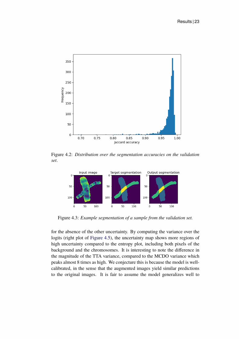
4.1 Segmentation accuracyThe results presented in Figure 4.1 show that the model hyperparameterswere adequately set, as the training is stable and no signs of overfitting orunderfitting are apparent. In Figure 4.2, we plot a histogram showing thedistribution of the segmentation accuracies on the validation set, obtained withthe final model after training for 40 epochs, due to both time-constraints andthe fact that training is more or less stagnant at this point. The mean value ofthe accuracies was 97.5 % with a standard deviation of 2.3 %.

4.2 Uncertainty EstimationsThis chapter is devoted to describing the results from the uncertainty estimation.We used the sample in Figure 4.3 6 to qualitatively demonstrate the differentuncertainty metrics by plotting the resulting uncertainty maps. Moreover, wewill use PCC to quantitatively describe the relation between the uncertaintyand the accuracy of the segmentation.

22 | Results

Figure 4.1: Training and validations results in terms of loss and segmentationduring the training phase of the U-Net.

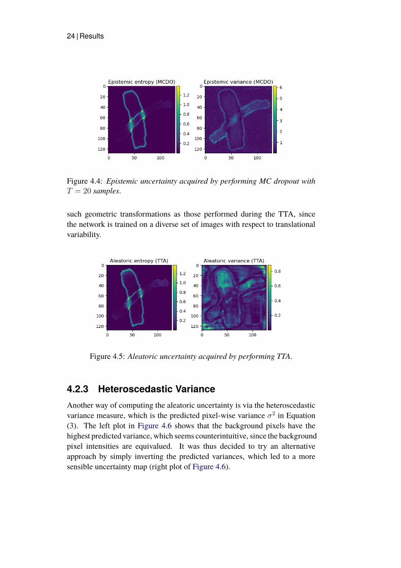
4.2.1 Monte Carlo DropoutThe epistemic uncertainty is measured by performing MC dropout with T =

20 MC samples. The uncertainty maps in Figure 4.4 show the epistemicentropy to the left and the epistemic variance to the right. The pixelsoutlining the boundaries of the chromosomes are naturally more difficult toclassify than pixels far away from the boundaries and thus the uncertainty ishigher. Likewise, the overlapping region shows a higher uncertainty both usingentropy and variance as a measure. One qualitative distinction between theentropy and the variance plot is that the interior pixels of the chromosomes aswell as the background show overall higher uncertainty for the variance.

4.2.2 Test Time AugmentationFirst, we note from the left plot of Figure 4.5 that the entropy uncertainty mapis highly similar to that of the epistemic entropy, both in terms of magnitudeand the regions that show high uncertainty. As suggested in [3], if only onesource of uncertainty is explicitly modeled, it seems to attempt compensating

Results | 23

Figure 4.2: Distribution over the segmentation accuracies on the validationset.

Figure 4.3: Example segmentation of a sample from the validation set.

for the absence of the other uncertainty. By computing the variance over thelogits (right plot of Figure 4.5), the uncertainty map shows more regions ofhigh uncertainty compared to the entropy plot, including both pixels of thebackground and the chromosomes. It is interesting to note the difference inthe magnitude of the TTA variance, compared to the MCDO variance whichpeaks almost 8 times as high. We conjecture this is because the model is well-calibrated, in the sense that the augmented images yield similar predictionsto the original images. It is fair to assume the model generalizes well to

24 | Results

Figure 4.4: Epistemic uncertainty acquired by performing MC dropout withT = 20 samples.

such geometric transformations as those performed during the TTA, sincethe network is trained on a diverse set of images with respect to translationalvariability.

Figure 4.5: Aleatoric uncertainty acquired by performing TTA.

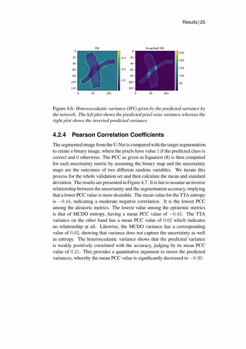
4.2.3 Heteroscedastic VarianceAnother way of computing the aleatoric uncertainty is via the heteroscedasticvariance measure, which is the predicted pixel-wise variance σ2 in Equation(3). The left plot in Figure 4.6 shows that the background pixels have thehighest predicted variance, which seems counterintuitive, since the backgroundpixel intensities are equivalued. It was thus decided to try an alternativeapproach by simply inverting the predicted variances, which led to a moresensible uncertainty map (right plot of Figure 4.6).

Results | 25

Figure 4.6: Heteroscedastic variance (HV) given by the predicted variance bythe network. The left plot shows the predicted pixel-wise variance whereas theright plot shows the inverted predicted variance.

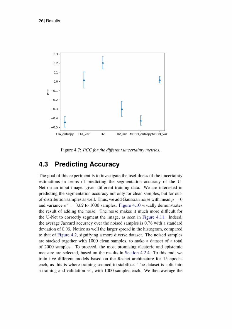
4.2.4 Pearson Correlation CoefficientsThe segmented image from theU-Net is comparedwith the target segmentationto create a binary image, where the pixels have value 1 if the predicted class iscorrect and 0 otherwise. The PCC as given in Equation (8) is then computedfor each uncertainty metric by assuming the binary map and the uncertaintymaps are the outcomes of two different random variables. We iterate thisprocess for the whole validation set and then calculate the mean and standarddeviation. The results are presented in Figure 4.7. It is fair to assume an inverserelationship between the uncertainty and the segmentation accuracy, implyingthat a lower PCC value is more desirable. The mean value for the TTA entropyis −0.44, indicating a moderate negative correlation. It is the lowest PCCamong the aleatoric metrics. The lowest value among the epistemic metricsis that of MCDO entropy, having a mean PCC value of −0.43. The TTAvariance on the other hand has a mean PCC value of 0.02 which indicatesno relationship at all. Likewise, the MCDO variance has a correspondingvalue of 0.02, showing that variance does not capture the uncertainty as wellas entropy. The heteroscedastic variance shows that the predicted varianceis weakly positively correlated with the accuracy, judging by its mean PCCvalue of 0.21. This provides a quantitative argument to invert the predictedvariances, whereby the mean PCC value is significantly decreased to −0.30.

26 | Results

Figure 4.7: PCC for the different uncertainty metrics.

4.3 Predicting AccuracyThe goal of this experiment is to investigate the usefulness of the uncertaintyestimations in terms of predicting the segmentation accuracy of the U-Net on an input image, given different training data. We are interested inpredicting the segmentation accuracy not only for clean samples, but for out-of-distribution samples as well. Thus, we addGaussian noise withmean µ = 0

and variance σ2 = 0.02 to 1000 samples. Figure 4.10 visually demonstratesthe result of adding the noise. The noise makes it much more difficult forthe U-Net to correctly segment the image, as seen in Figure 4.11. Indeed,the average Jaccard accuracy over the noised samples is 0.78 with a standarddeviation of 0.06. Notice as well the larger spread in the histogram, comparedto that of Figure 4.2, signifying a more diverse dataset. The noised samplesare stacked together with 1000 clean samples, to make a dataset of a totalof 2000 samples. To proceed, the most promising aleatoric and epistemicmeasure are selected, based on the results in Section 4.2.4. To this end, wetrain five different models based on the Resnet architecture for 15 epochseach, as this is where training seemed to stabilize. The dataset is split intoa training and validation set, with 1000 samples each. We then average the

Results | 27

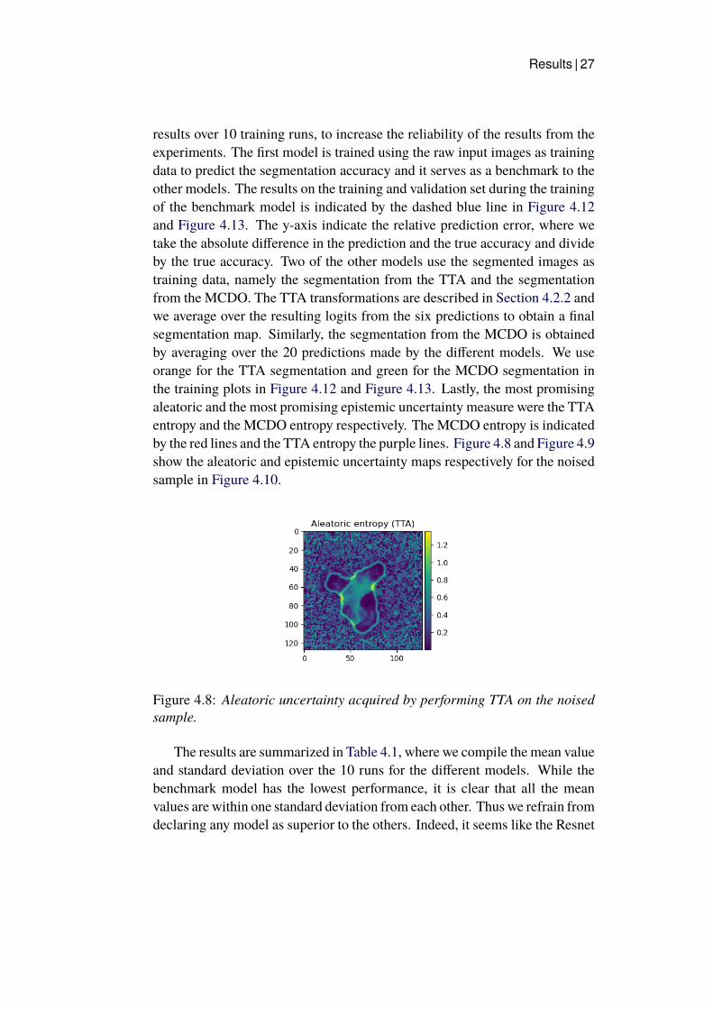
results over 10 training runs, to increase the reliability of the results from theexperiments. The first model is trained using the raw input images as trainingdata to predict the segmentation accuracy and it serves as a benchmark to theother models. The results on the training and validation set during the trainingof the benchmark model is indicated by the dashed blue line in Figure 4.12and Figure 4.13. The y-axis indicate the relative prediction error, where wetake the absolute difference in the prediction and the true accuracy and divideby the true accuracy. Two of the other models use the segmented images astraining data, namely the segmentation from the TTA and the segmentationfrom the MCDO. The TTA transformations are described in Section 4.2.2 andwe average over the resulting logits from the six predictions to obtain a finalsegmentation map. Similarly, the segmentation from the MCDO is obtainedby averaging over the 20 predictions made by the different models. We useorange for the TTA segmentation and green for the MCDO segmentation inthe training plots in Figure 4.12 and Figure 4.13. Lastly, the most promisingaleatoric and the most promising epistemic uncertainty measure were the TTAentropy and the MCDO entropy respectively. The MCDO entropy is indicatedby the red lines and the TTA entropy the purple lines. Figure 4.8 and Figure 4.9show the aleatoric and epistemic uncertainty maps respectively for the noisedsample in Figure 4.10.

Figure 4.8: Aleatoric uncertainty acquired by performing TTA on the noisedsample.

The results are summarized in Table 4.1, where we compile the mean valueand standard deviation over the 10 runs for the different models. While thebenchmark model has the lowest performance, it is clear that all the meanvalues are within one standard deviation from each other. Thus we refrain fromdeclaring any model as superior to the others. Indeed, it seems like the Resnet

28 | Results

Figure 4.9: Epistemic uncertainty acquired by performing MCDO with T =20 MC samples.

Training data Mean Standard deviationInput img 0.041 0.012TTA seg 0.033 0.0056

MCDO seg 0.040 0.017MCDO entropy 0.036 0.0063TTA entropy 0.035 0.0094

Table 4.1: Mean relative validation error after 15 epochs together with thecorresponding standard deviation for the five different ResNet models.

models are more or less equally apt to predict the segmentation accuracyand that there is no significant benefit of using the uncertainty estimations.We conjecture that this finding is partly explained by the artificial way ofgenerating out-of-distribution samples. Indeed, it may be the case that theResnet models simply learn to detect the noise and correlate the amount ofnoise with the accuracy. The benefits of using the uncertainty estimationswould likely be more apparent if the dataset were more diverse in terms ofdifferent poor segmentations.

Results | 29

Figure 4.10: Example of a noised sample, together with the target and outputsegmentation.

Figure 4.11: Distribution over the segmentation accuracies on the noisedsamples.

30 | Results

Figure 4.12: Heteroscedastic aleatoric uncertainty given by the predictedvariance by the network.

Results | 31

Figure 4.13: Heteroscedastic aleatoric uncertainty given by the predictedvariance by the network.

32 | Results

Discussion | 33

Chapter 5

Discussion

Let us discuss the results of this thesis. Looking at Figure 4.1, we see that thetraining of the U-Net was stable and achieved satisfactory results in terms ofsegmentation accuracy. Indeed, Figure 4.2 reaffirms this notion and indicatesthat the model generalizes well over the validation set, with comparablyfew samples being inadequately segmented. However, we acknowledge thatthe dataset is rather limited in the sense that the only data augmentationtechniques used were rotations and translations, whereas more sophisticatedtransformations should be included for a more ubiquitous model.

At first glance, the epistemic uncertaintymaps in Figure 4.4 show qualitativepromise. For the entropy measure, we note that the boundaries indicatea relative high uncertainty, but only for the chromosome with label 1. Itwould be interesting to further investigate this finding, however, the limitedtime did not allow for more thorough experiments. On the other hand, theepistemic variance over the logits show a similar level of uncertainty forboth chromosomes. A possible explanation is that the distribution over thepredicted classes is more unimodal for the chromosome on top, which wouldlead to a high variance but low entropy, but a quantitative argument would beneeded to further strengthen this idea.

When we studied the aleatoric uncertainty, we see that the entropy ofthe probability distributions induced by TTA in the left plot of Figure 4.5looks almost identitical to the epistemic entropy. While there is evidence[3] that suggests that in the absence of the other, epistemic and aleatoricbased methods capture the same uncertainty, we did not aim to systematicallycompare the differences in what they measure. There are less similaritiesbetween the epistemic and aleatoric uncertainty, as measured by MCDO andTTA respectively, in terms of the variance metrics. First of all, there is a

34 | Discussion

significantly larger peak in magnitude for the epistemic variance, althoughmore regions show a relatively high uncertainty for the aleatoric variance.Regarding the heteroscedastic variance, which is plotted in Figure 4.6, wefound that the predicted variance resulted in a contradictory uncertainty map,where the background pixels show the highest uncertainty. While this couldbe due to a faulty implementation, we speculate that the U-Net tends to assigncomparably high values of σ to easily classifiable pixels, since this does notaffect the final classification given that the correct class has a high activityin the output node. Nevertheless, by inverting the predicted variance, seenin the right plot of Figure 4.6, we see a segmentation map that more closelyresembles the ones achieved with MCDO and TTA.

Overall, we observed how the entropy measures performed considerablybetter in terms of correlating with the segmentation accuracy compared to thevariance measures, as seen in Figure 4.7. We hypothesize that the distributionover the predicted classes is more or less multimodal, at least over the regionscovered by the chromosomes, since they have comparable pixel intensities.As such, variance being a central tendency measure is rather uninformativeand entropy is thus preferred. We also note how the heteroscedastic variancescores a positive correlation, which contradicts the reasonable expectation thatuncertainty negatively correlates with accuracy. The inverted heteroscedasticvariance on the other hand yields a negative correlation and may thus beinterpreted as a more favorable measure for this particular dataset and choiceof model.

In section 4.3, we were interested in first predicting the accuracy of bothregular samples and out-of-distribution samples. By plotting the distributionover the segmentation accuracies on the noised samples in Figure 4.11, wedemonstrate the difficulty of correctly segmenting these out-of-distributionsamples. We chose TTA entropy and MCDO entropy to measure the aleatoricand epistemic uncertainty and judging from Figure 4.8 and Figure 4.9, theyseem to produce quite similar uncertainty maps. This makes sense, since theaugmented data could be interpreted both as containing inherent data noise,which is captured by TTA, and as being out-of-distribution, which is capturedby MCDO. The values in Table 4.1 indicated that the uncertainty maps werenot on average more informative than the actual segmentations or even theoriginal input image. Keeping in mind that the goal of this experiment wasto predict the segmentation accuracy for both good and poor segmentations,we believe the dataset in question was simply not diverse enough for theuncertainty measures to prove useful.

Conclusions and Future work | 35

Chapter 6

Conclusions and Future work

This chapter is devoted to summarize what was achieved in this degreeproject. An overview of the results from the segmentation task, the uncertaintyestimations and the task of predicting the segmentation accuracy are given inSection 6.1, while Section 6.2 outlines potential avenues for future work whichcould either improve the results or provide new interesting insights to the topic.

6.1 ConclusionsWe showed that our proposed implementation of the U-Net was able toaccurately segment pairs of overlapping chromosomes, with a validationaccuracy of 97.5 %. However, this comes with the caveat of evaluating thenetwork on a synthetically generated overlaps, whereas the performance onauthentic overlapping chromosomes is left for future work. We then evaluatedthe usefulness of different uncertainty metrics to predict the segmentationaccuracy in terms of the PCC. Firstly, we observed entropy to be moresuitable than variance in this context and accounted the possibly multimodalprobability distribution for this finding. Secondly, our findings showed thatthere was no significant difference in the relative predicted segmentationaccuracy between the models in Table 4.1.

6.2 Future WorkThere are a number of potentially interesting research points. The first pointis to synthetically create an augmented dataset of overlapping chromosomeswhich to a higher degree resemble authentic overlaps. For example, a

36 | Conclusions and Future work

possible approach would be to convolve the image with a low-pass filtersuch as Gaussian blur, in order to smoothen the overlapping region. Amore sophisticated method involves employing a generative adversial networktrained on a set of images containing actual overlapping chromosomes toaugment the dataset with samples from the same distribution as the onetraining data.

Furthermore, one may consider using another network architecture for thesegmentation task. Indeed, we choseU-Net for its simplicity in implementation,making it suitable for adding dropout layers and making use of the learningloss attenuation. On the other hand, this choice of network restricted thesegmentation task to one of semantic as opposed to instance segmentation.While the labels in semantic segmentation are class-aware, the labels ininstance segmentation are instance-aware. Thus, if one considers the chromosomesto be of the same class, it makes more sense to opt for a network more suitablefor instance segmentation, such as Mask R-CNN.

While this thesis did cover a fair number of different uncertainty metrics,there is still more to discover. Indeed, another common approach to measureuncertainty in image classification tasks is deep ensemble learning, whichis a technique used to quantify predictive uncertainty estimation in NNs.In 2016, a research team at DeepMind demonstrated how deep ensemblelearning can outperform or match Bayesian NNs in both regression andclassification tasks, citing its simple implementation and scalability as someof the advantages [30]. One could also investigate whether the assumptionthat epistemic uncertainty is inversely correlated with the size of the trainingset holds true, as a sort of sanity check. Of more practical use, it should beof interest to systematically survey when and for what kind of samples it ismore advantageous to measure the aleatoric uncertainty than the epistemicuncertainty and vice versa, or whether there is a practical and robust way ofcombining them.

One should also be implored to explore differentmethods of producing out-of-distribution samples, to better understand when and why the segmentationfails. Ideally, the dataset should include the sort of samples which are likely tooccur during test-time, which could include for example images containingmore than two chromosomes, cropped images and color-adjusted images.Lastly, it may be more convenient to harness the uncertainty maps to classifysamples as either adequately or inadequately segmented, rather than predictingthe segmentation accuracy.

REFERENCES | 37

References

[1] O. Ronneberger, P. Fischer, and T. Brox, “U-net: Convolutional networksfor biomedical image segmentation,” arXiv:1505.04597, 2015.

[2] K. He, X. Zhang, S. Ren, and J. Sun, “Deep residual learning for imagerecognition,” 2015.

[3] A. Kendall and Y. Gal, “What uncertainties do we need in bayesian deeplearning for computer vision?” arXiv:1703.04977v2, 2017.

[4] J. Manjunath, M. Mohana, M. Madhulika, G. Divya, R. Meghana,and S. Apoorva, “Feature extraction using convolution neuralnetworks (cnn) and deep learning,” pp. 2319–2323, 05 2018. doi:10.1109/RTEICT42901.2018.9012507

[5] L. L. Ankile, M. F. Heggland, and K. Krange, “Deep convolutionalneural networks: A survey of the foundations, selected improvements,and some current applications,” 2020.

[6] L. SB, L. SA, L. JS, F. MT, C. MV, and M. SK, “Artificial convolutionneural network techniques and applications for lung nodule detection,”IEEE Trans Med Imaging, 1995. doi: 10.1109/42.476112

[7] A. Krizhevsky, I. Sutskever, and G. E. Hinton, “Imagenet classificationwith deep convolutional neural networks,” in Advances in NeuralInformation Processing Systems, F. Pereira, C. J. C. Burges, L. Bottou,and K. Q. Weinberger, Eds., vol. 25. Curran Associates, Inc.,2012. [Online]. Available: https://proceedings.neurips.cc/paper/2012/file/c399862d3b9d6b76c8436e924a68c45b-Paper.pdf

[8] Y. Bengio, P. Simard, and P. Frasconi, “Learning long-termdependencies with gradient descent is difficult,” IEEE Transactionson Neural Networks, vol. 5, no. 2, pp. 157–166, 1994. doi:10.1109/72.279181

38 | REFERENCES

[9] F. Laumann. [Online]. Available: https://towardsdatascience.com/what-uncertainties-tell-you-in-bayesian-neural-networks-6fbd5f85648e

[10] W. et al., “Aleatoric uncertainty estimation with test-time augmentationfor medical image segmentation with convolutional neural networks,”Neurocomputing 338 (2019) 34–45, 2019.

[11] D. Shanmugam, D. Blalock, G. Balakrishnan, and J. Guttag, “When andwhy test-time augmentation works,” 2020.

[12] J. Brownlee. [Online]. Available: https://machinelearningmastery.com/dropout-for-regularizing-deep-neural-networks/

[13] T. D. et al., “Leveraging uncertainty estimates for predictingsegmentation quality,” arXiv: 1807.00502v1, 2018.

[14] M. I. J. et al., “An introduction to variational methods for graphicalmodels,” Machine learning, 37(2):183–233, 1999.

[15] L. Perez and J. Wang, “The effectiveness of data augmentation in imageclassification using deep learning,” 2017.

[16] C. Shorten and T. M. Khoshgoftaar, “A survey on image dataaugmentation for deep learning,” Mathematics and Computers inSimulation. Springer. 6: 60. doi: 10.1186/s40537-019-0197-0

[17] P. K. Gadosey, Y. Li, and E. A. Agyekum, “Sd-unet: Stripping downu-net for segmentation of biomedical images on platforms with lowcomputational budgets,” 2020. doi: 10.3390/diagnostics10020110

[18] H. M. Saleh, N. H. Saad, and N. A. M. Isa, “Overlapping chromosomesegmentation using u-net: Convolutional networks with test timeaugmentation,” Procedia Computer Science, 2019.

[19] J. Pommier. [Online]. Available: https://github.com/jeanpat/DeepFISH/tree/master/dataset

[20] H. et al., “Image segmentation to distinguish between overlapping humanchromosomes,” Information Processing Systems Machine Learning forHealth Workshop, 2017.

[21] H. B. et al., “Chromosome extraction based on u-net andyolov3,” IEEE Access, vol. 8, pp. 178563-178569, 2020. doi:10.1109/ACCESS.2020.3026483

REFERENCES | 39

[22] J. Redmon and A. Farhadi, “Yolov3: An incremental improvement,”arXiv, 2018.

[23] G. G. e. a. K. He, “Mask r-cnn,” Proc. IEEE Int. Conf. Comput. Vis., Oct.2017, pp. 29802988, 2017.

[24] H. Z. et al., “Pyramid scene parsing network,” arXiv:1612.01105, 2016.

[25] P. C. et al., “Chromosome segmentation via data simulation andshape learning,” Annu Int Conf IEEE Eng Med Biol Soc., 2020. doi:10.1109/EMBC44109.2020.9176020

[26] X.-Y. Zhou and G.-Z. Yang, “Normalization in training u-net for 2dbiomedical semantic segmentation,” 2019.

[27] A. F. Agarap, “Deep learning using rectified linear units (relu),” 2019.

[28] Y. Gal and Z. Ghahramani, “Dropout as a bayesian approximation:Representingmodel uncertainty in deep learning,” arXiv: 1506.02142v6,2016.

[29] R. Seoh, “Qualitative analysis of monte carlo dropout,” 2020.

[30] B. Lakshminarayanan, A. Pritzel, and C. Blundell, “Simple and scalablepredictive uncertainty estimation using deep ensembles,” 2017.

40 | REFERENCES

For DIVA{"Author1": {

"Last name": "Norström","First name": "Arvid","Local User Id": "arvidno","E-mail": "arvidno@kth.se",

},"Degree": {"Educational program": "Master’s Programme, Machine Learning, 120 credits"},"Title": {

"Main title": "Deep Learning for Chromosome Segmentation with Uncertainty Estimation","Language": "eng" },

"Alternative title": {"Main title": "Djupinlärning för Kromosomsegmentering med Osäkerhetsestimation","Language": "swe"

},"Supervisor1": {

"Last name": "Björkman","First name": "Mårten","Local User Id": "celle","E-mail": "celle@kth.se","organisation": {"L1": "School of Electrical Engineering and Computer Science ",

"L2": "Computer Science" }},

"Examiner1": {"Last name": "Kragíc Jensfelt","First name": "Danica","Local User Id": "danik","E-mail": "danik@kth.se","organisation": {"L1": "School of Electrical Engineering and Computer Science ",

"L2": "Computer Science" }},

"Cooperation": { "Partner_name": "Arkus AI"},"Other information": {"Year": "2021", "Number of pages": "1,41"}}

www.kth.se

TRITA -EECS-EX-2021:542