Deep learning for neuroimaging: a validation study

Sergey M. PlisThe Mind Research Network

Albuquerque, NM 87106s.m.plis@gmail.com

Devon R. HjelmUniversity of New MexicoAlbuquerque, NM 87131dhjelm@mrn.org

Ruslan SalakhutdinovUniversity of Toronto

Toronto, Ontario M5S 2E4rsalakhu@cs.toronto.edu

Vince D. CalhounThe Mind Research Network

Albuquerque, NM 87106vcalhoun@mrn.org

Abstract

Deep learning methods have recently made notable advances in the tasks of clas-sification and representation learning. These tasks are important for brain imag-ing and neuroscience discovery, making the methods attractive for porting to aneuroimager’s toolbox. Success of these methods is, in part, explained by theflexibility of deep learning models. However, this flexibility makes the processof porting to new areas a difficult parameter optimization problem. In this workwe demonstrate our results (and feasible parameter ranges) in application of deeplearning methods to structural and functional brain imaging data. We also describea novel constraint-based approach to visualizing high dimensional data. We useit to ana- lyze the effect of parameter choices on data transformations. Our re-sults show that deep learning methods are able to learn physiologically importantrepresentations and detect latent relations in neuroimaging data.

1 Introduction

One of the main goals of brain imaging and neuroscience—and, possibly, of most natural sciences—is to improve understanding of the investigated system based on data. In our case, this amounts toinference of descriptive features of brain structure and function from non-invasive measurements.Brain imaging field has come a long way from anatomical maps and atlases towards data driven fea-ture learning methods, such as seed-based correlation [2], canonical correlation analysis [33], andindependent component analysis (ICA) [1, 24]. These methods are highly successful in revealingknown brain features with new details [3] (supporting their credibility), in recovering features thatdifferentiate patients and controls [28] (assisting diagnosis and disease understanding), and startinga “resting state” revolution after revealing consistent patters in data from uncontrolled resting ex-periments [29, 35]. Classification is often used merely as a correctness checking tool, as the mainemphasis is on learning about the brain. A perfect oracle that does not explain its conclusions wouldbe useful, but mainly to facilitate the inference of the ways the oracle draws these conclusions.

As an oracle, deep learning methods are breaking records taken over the areas of speech, signal,image, video and text mining and recognition by improving state of the art classification accuracyby, sometimes, more than 30% where the prior decade struggled to obtain a 1-2% improvements [19,21]. What differentiates them from other classifiers, however, is the automatic feature learning fromdata which largely contributes to improvements in accuracy. Presently, this seems to be the closestsolution to an oracle that reveals its methods — a desirable tool for brain imaging.

Another distinguishing feature of deep learning is the depth of the models. Based on already ac-ceptable feature learning results obtained by shallow models—currently dominating neuroimaging

1

arX

iv:1

312.

5847

v3 [

cs.N

E]

19

Feb

2014

field—it is not immediately clear what benefits would depth have. Considering the state of multi-modal learning, where models are either assumed to be the same for analyzed modalities [26] orcross-modal relations are sought at the (shallow) level of mixture coefficients [23], deeper modelsbetter fit the intuitive notion of cross-modality relations, as, for example, relations between geneticsand phenotypes should be indirect, happening at a deeper conceptual level.

In this work we present our recent advances in application of deep learning methods to functionaland structural magnetic resonance imaging (fMRI and sMRI). Each consists of brain volumes but forsMRI these are static volumes—one per subject/session,—while for fMRI a single subject datasetis comprised of multiple volumes capturing the changes during an experimental session. Our goalis to validate feasibility of this application by a) investigating if a building block of deep generativemodels—a restricted Boltzmann machine (RBM) [17]—is competitive with ICA (a representativemodel of its class) (Section 2); b) examining the effect of the depth in deep learning analysis ofstructural MRI data (Section 3.3); and c) determining the value of the methods for discovery of latentstructure of a large-scale (by neuroimaging standards) dataset (Section 3.4). The measure of featurelearning performance in a shallow model (a) is comparable with existing methods and known brainphysiology. However, this measure cannot be used when deeper models are investigated. As wefurther demonstrate, classification accuracy does not provide the complete picture either. To be ableto visualize the effect of depth and gain an insight into the learning process, we introduce a flexibleconstraint satisfaction embedding method that allows us to control the complexity of the constraints(Section 3.2). Deliberately choosing local constraints we are able to reflect the transformations thatthe deep belief network (DBN) [15] learns and applies to the data and gain additional insight.

2 A shallow belief network for feature learning

Prior to investigating the benefits of depth of a DBN in learning representations from fMRI andsMRI data, we would like to find out if a shallow (single hidden layer) model–which is the RBM—from this family meets the field’s expectations. As mentioned in the introduction, a number ofmethods are used for feature learning from neuroimaging data: most of them belong to the singlematrix factorization (SMF) class. We do a quick comparison to a small subset of SMF methods onsimulated data; and continue with a more extensive comparison against ICA as an approach trustedin the neuroimaging field. Similarly to RBM, ICA relies on the bipartite graph structure, or evenis an artificial neural network with sigmoid hidden units as is in the case of Infomax ICA [1] thatwe compare against. Note the difference with RBM: ICA applies its weight matrix to the (shorter)temporal dimension of the data imposing independence on the spatial dimension while RBM appliesits weight matrix (hidden units “receptive fields”) to the high dimensional spatial dimension instead(Figure 2).

2.1 A restricted Boltzmann machine

A restricted Boltzmann machine (RBM) is a Markov random field that models data distributionparameterizing it with the Gibbs distribution over a bipartite graph between visible v and hiddenvariables h [10]: p(v) =

∑h p(v,h) =

∑h 1/Z exp(−E(v,h)), where Z =

∑v∑

h e−E(v,h)

is the normalization term (the partition function) and E(v,h) is the energy of the system. Eachvisible variable in the case of fMRI data represents a voxel of an fMRI scan with a real-valued andapproximately Gaussian distribution. In this case, the energy is defined as:

E(v,h) = −∑ij

vjσjWjihi −

∑j

(aj − vj)2

σ2j

−∑i

bihi, (1)

where aj and bj are biases and σj is the standard deviation of a parabolic containment function foreach visible variable vj centered on the bias aj . In general, the parameters σi need to be learnedalong with the other parameters. However, in practice normalizing the distribution of each voxel tohave zero mean and unit variance is faster and yet effective [27]. A number of choices affect thequality of interpretation of the representations learned from fMRI by an RBM. Encouraging sparsefeatures via the L1-regularization: λ‖W‖1 (λ = 0.1 gave best results) and using hyperbolic tangentfor hidden units non-linearity are essential settings that respectively facilitate spatial and temporalinterpretation of the result. The weights were updated using the truncated Gibbs sampling method

2

called contrastive divergence (CD) with a single sampling step (CD-1). Further information on RBMmodel can be found in [16, 17].

2.2 Synthetic dataCo

rrel

atio

n

Spatial Maps Time Courses

0

0.9

a: Average spatial map (SM) andtime course (TC) correlations toground truth for RBM and SMFmodels (gray box).

GT RBM ICA

b: Ground truth (GT) SMs andestimates obtained by RBM andICA (thresholded at 0.4 height).Colors are consistent across themethods. Grey indicates back-ground or areas without SMsabove threshold.

Hig

her i

s be

tter

Hig

her i

s be

tter

Low

er is

bet

ter ICA

RBM

c: Spatial, temporal, and cross correla-tion (FNC) accuracy for ICA (red) andRBM (blue), as a function of spatialoverlap of the true sources from 1b.Lines indicate the average correlationto GT, and the color-fill indicates ±2standard errors around the mean.

Figure 1: Comparison of RBM estimation accuracy of features and their time courses with SMFs.

In this section we summarize our comparisons of RBM with SMF models—including InfomaxICA [1], PCA [14], sparse PCA (sPCA) [37], and sparse NMF (sNMF) [18]—on synthetic datawith known spatial maps generated to simulate fMRI.

Figure 1a shows the correlation of spatial maps (SM) and time course (TC) estimates to the groundtruth for RBM, ICA, PCA, sPCA, and sNMF. Correlations are averaged across all sources anddatasets. RBM and ICA showed the best overall performance. While sNMF also estimated SMswell, it showed inferior performance on TC estimation, likely due to the non-negativity constraint.Based on these results and the broad adoption of ICA in the field, we focus on comparing InfomaxICA and RBM.

Figure 1b shows the full set of ground truth sources along with RBM and ICA estimates for a singlerepresentative dataset. SMs are thresholded and represented as contours for visualization. Resultsover all synthetic datasets showed similar performance for RBM and ICA (Figure 1c), with a slightadvantage for ICA with regard to SM estimation, and a slight advantage for RBM with regards toTC estimation. RBM and ICA also showed comparable performance estimating cross correlationsalso called functional network connectivity (FNC).

2.3 An fMRI data application

fMRI dataRBM training

Time coursesTarget time courseRBM Features

Cross correlations

Task-related features

Feat

ures

Space

xx =

TRAINING

fMRI data

ANALYSIS Time

Spac

e

Figure 2: The processes of feature learning and time course computation from fMRI data by anRBM. The visible units are voxels and a hidden unit receptive field covers an fMRI volume.

Data used in this work comprised of task-related scans from 28 (five females) healthy participants, allof whom gave written, informed, IRB-approved consent at Hartford Hospital and were compensatedfor participation1. All participants were scanned during an auditory oddball task (AOD) involvingthe detection of an infrequent target sound within a series of standard and novel sounds2.

1More detailed information regarding participant demographics is provided in [9]2The task is described in more detail in [4] and [9].

3

Scans were acquired at the Olin Neuropsychiatry Research Center at the Institute of Living/HartfordHospital on a Siemens Allegra 3T dedicated head scanner equipped with 40 mT/m gradients and astandard quadrature head coil [4, 9]. The AOD consisted of two 8-min runs, and 249 scans (volumes)at 2 second TR (0.5 Hz sampling rate) were used for the final dataset. Data were post-processedusing the SPM5 software package [12], motion corrected using INRIalign [11], and subsampled to53 × 63 × 46 voxels. The complete fMRI dataset was masked below mean and the mean imageacross the dataset was removed, giving a complete dataset of size 70969 voxels by 6972 volumes.Each voxel was then normalized to have zero mean and unit variance.

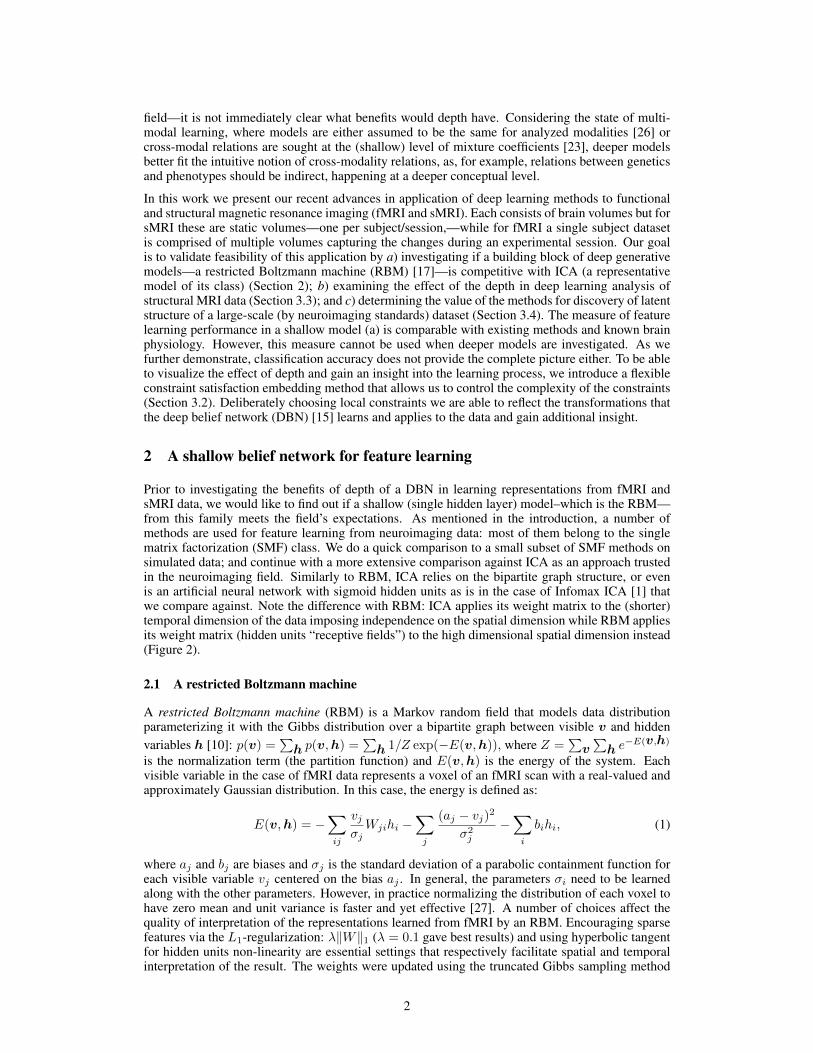
Figure 3: Intrinsic brain networksestimated by ICA and RBM.

The RBM was constructed using 70969 Gaussian visibleunits and 64 hyperbolic tangent hidden units. The hyperparameters ε (0.08 from the searched [1× 10−4, 1× 10−1]range) for learning rate and λ (0.1 from the searched range[1× 10−2,1× 10−1]) for L1 weight decay were selected asthose that showed a reduction of reconstruction error overtraining and a significant reduction in span of the receptivefields respectively. Parameter value outside the ranges eitherresulted in unstable or slow learning (ε) or uninterpretable fea-tures (λ). The RBM was then trained with a batch size of 5for approximately 100 epochs to allow for full convergence ofthe parameters.

After flipping the sign of negative receptive fields, we then identified and labeled spatially distinctfeatures as corresponding to brain regions with the aid of AFNI [5] excluding features which had ahigh probability of corresponding to white matter, ventricles, or artifacts (eg. motion, edges).

We normalized the fMRI volume time series to mean zero and used the trained RBM in feed-forwardmode to compute time series for each fMRI feature. This was done to better compare to ICA, wherethe mean is removed in PCA preprocessing.

The work-flow is outlined in Figure 2, while Figure 3 shows comparison of resulting featureswith those obtained by Infomax ICA. In general, RBM performs competitively with ICA, whileproviding–perhaps, not surprisingly due to the used L1 regularization—sharper and more local-ized features. While we recognize that this is a subjective measure we list more features in Fig-ure S2 of Section 5 and note that RBM features lack negative parts for corresponding features.Note, that in the case of L1 regularized weights RBM algorithms starts to resemble some ofthe ICA approaches (such as the recent RICA by Le at al. [20]), which may explain the sim-ilar performance. However, the differences and possible advantages are the generative natureof the RBM and no enforcement of component orthogonality (not explicit at the least). More-over, the block structure of the correlation matrix (see below the Supplementary material section)of feature time courses provide a grouping that is more physiologically supported than that pro-vided by ICA. For example, see Figure S1 in the supplementary material section below. Perhaps,because ICA working hard to enforce spatial independence subtly affects the time courses andtheir cross-correlations in turn. We have observed comparable running times of the (non GPU)ICA (http://www.nitrc.org/projects/gift) and a GPU implementation of the RBM(https://github.com/nitishsrivastava/deepnet).

3 Validating the depth effect

Since the RBM results demonstrate a feature-learning performance competitive with the state of theart (or better), we proceed to investigating the effects of the model depth. To do that we turn fromfMRI to sMRI data. As it is commonly assumed in the deep learning literature [22] the depth is oftenimproving classification accuracy. We investigate if that is indeed true in the sMRI case. Structuraldata is convenient for the purpose as each subject/session is represented only by a single volume thathas a label: control or patient in our case. Compare to 4D data where hundreds of volumes belongto the same subject with the same disease state.

3.1 A deep belief network

A DBN is a sigmoidal belief network (although other activation functions may be used) with anRBM as the top level prior. The joint probability distribution of its visible and hidden units is

4

parametrized as follows:

P (v,h1,h2, . . . ,hl) = P (v|h1)P (h1|h2) · · ·P (hl−2,hl−1)P (hl−1,hl), (2)

where l is the number of hidden layers, P (hl−1,hl) is an RBM, and P (hi|hi+1) factor into indi-vidual conditionals:

P (hi|hi+1) =

ni∏j=1

P (hij |hi+1) (3)

The important property of DBN for our goals of feature learning to facilitate discovery is its ability tooperate in generative mode with fixed values on chosen hidden units thus allowing one to investigatethe features that the model have learned and/or weighs as important in discriminative decisions.We, however, not going to use this property in this section, focusing instead on validating the claimthat a network’s depth provides benefits for neuroimaging data analysis. And we will do this usingdiscriminative mode of DBN’s operation as it provides an objective measure of the depth effect.

DBN training splits into two stages: pre-training and discriminative fine tuning. A DBN can bepre-trained by treating each of its layers as an RBM—trained in an unsupervised way on inputsfrom the previous layer—and later fine-tuned by treating it as a feed-forward neural network. Thelatter allows supervised training via the error back propagation algorithm. We use this schema in thefollowing by augmenting each DBN with a soft-max layer at the fine-tuning stage.

3.2 Nonlinear embedding as a constraint satisfaction problem

A DBN and an RBM operate on data samples, which are brain volumes in the fMRI and sMRIcase. A five-minute fMRI experiment with 2 seconds sampling rate yields 150 of these volumes persubject. For sMRI studies number of participating subjects varies but in this paper we operate witha 300 and a 3500 subject-volumes datasets. Transformations learned by deep learning methods donot look intuitive in the hidden node space and generative sampling of the trained model does notprovide a sense if a model have learned anything useful in the case of MRI data: in contrast to naturalimages, fMRI and sMRI images do not look very intuitive. Instead, we use a nonlinear embeddingmethod to control whether a model learned useful information and to assist in investigation of whathave it, in fact, learned.

One of the purposes of an embedding is to display a complex high dimensional dataset in a waythat is i) intuitive, and ii) representative of the data sample. The first requirement usually leads todisplaying data samples as points in a 2-dimensional map, while the second is more elusive andeach approach addresses it differently. Embedding approaches include relatively simple randomlinear projections—provably preserving some neighbor relations [6]—and a more complex classof nonlinear embedding approaches [30, 32, 34, 36]. In an attempt to organize the properties ofthis diverse family we have aimed at representing nonlinear embedding methods under a singleconstraint satisfaction problem (CSP) framework (see below). We hypothesize that each methodplaces the samples in a map to satisfy a specific set of constraints. Although this work is not yetcomplete, it proven useful in our current study. We briefly outline the ideas in this section to provideenough intuition of the method that we further use in Section 3.

Since we can control the constraints in the CSP framework, to study the effect of deep learning wechoose them to do the least amount of work—while still being useful—letting the DBN do (or not)the hard part. A more complicated method such as t-SNE [36] already does complex processingto preserve the structure of a dataset in a 2D map – it is hard to infer if the quality of the map isdetermined by a deep learning method or the embedding. While some of the existing method mayhave provided the “least amount of work” solutions as well we chose to go with the CSP framework.It explicitly states the constraints that are being satisfied and thus lets us reason about deep learningeffects within the constraints, while with other methods—where the constraints are implicit—thiswould have been harder.

A constraint satisfaction problem (CSP) is one requiring a solution that satisfies a set of constraints.One of the well known examples is the boolean satisfiability problem (SAT). There are multipleother important CSPs such as the packing, molecular conformations, and, recently, error correctingcodes [7]. Freedom to setup per point constraints without controlling for their global interactionsmakes a CSP formulation an attractive representation of the nonlinear embedding problem. Pursuing

5

this property we use the iterative “divide and concur” (DC) algorithm [13] as the solver for ourrepresentation. In DC algorithm we treat each point on the solution map as a variable and assign aset of constraints that this variable needs to satisfy (more on these later). Then each points gets a“replica” for each constraint it is involved into. Then DC algorithm alternates the divide and concurprojections. The divide projection moves each “replica” points to the nearest locations in the 2Dmap that satisfy the constraint they participate in. The concur projection concurs locations of all“replicas” of a point by placing them at the average location on the map. The key idea is to avoidlocal traps by combining the divide and concur steps within the difference map [8]. A single locationupdate is represented by:

xc = Pc((1 + 1/β) ∗ Pd(x)− 1/β ∗ x)xd = Pd((1− 1/β) ∗ Pc(x) + 1/β ∗ x)x = x+ β ∗ (xc − xd), (4)

where Pd(·) and Pc(·) denote the divide and concur projections and β is a user-defined parameter.

While the concur projection will only differ by subsets of “replicas” across different methods rep-resentable in DC framework, the divide projection is unique and defines the algorithm behavior. Inthis paper, we choose a divide projection that keeps k nearest neighbors of each point in the higherdimensional space also its neighbors in the 2D map. This is a simple local neighborhood constraintthat allows us to assess effects of deep learning transformation leaving most of the mapping deci-sions to the deep learning.

Note, that for a general dataset we may not be able to satisfy this constraint: each point has ex-actly the same neighbors in 2D as in the original space (and this is what we indeed observe). TheDC algorithm, however, is only guaranteed to find the solution if it exists and oscillates otherwise.Oscillating behavior is detectable and may be used to stop the algorithm. We found informativewatching the 2D map in dynamics, as the points that keep oscillating provide additional informationinto the structure of the data. Another practically important feature of the algorithm: it is determin-istic. Given the same parameters (β and the parameters of Pd(·)) it converges to the same solutionregardless of the initial point. If each of the points participates in each constraint then complex-ity of the algorithm is quadratic. With our simple k neighborhood constraints it is O(kn), for nsamples/points.

3.3 A schizophrenia structural MRI dataset

Figure 4: A smoothed gray matter seg-mentation of a patient and a healthycontrol: each is a training sample.

We use a combined data from four separate schizophreniastudies conducted at Johns Hopkins University (JHU), theMaryland Psychiatric Research Center (MPRC), the Insti-tute of Psychiatry, London, UK (IOP), and the WesternPsychiatric Institute and Clinic at the University of Pitts-burgh (WPIC) (the data used in Meda et al. [25]). Thecombined sample comprised 198 schizophrenia patientsand 191 matched healthy controls and contained both firstepisode and chronic patients [25]. At all sites, wholebrain MRIs were obtained on a 1.5T Signa GE scannerusing identical parameters and software. Original struc-tural MRI images were segmented in native space and theresulting gray and white matter images then spatially nor-malized to gray and white matter templates respectively toderive the optimized normalization parameters. These parameters were then applied to the wholebrain structural images in native space prior to a new segmentation. The obtained 60465 voxel graymatter images were used in this study. Figure 4 shows example orthogonal slice views of the graymatter data samples of a patient and a healthy control.

The main question of this Section is to evaluate the effect of the depth of a DBN on sMRI. Toanswer this question, we investigate if classification rates improve with the depth. For that wesequentially investigate DBNs of 3 depth. From RBM experiments we have learned that even witha larger number of hidden units (72, 128 and 512) RBM tends to only keep around 50 featuresdriving the rest to zero. Classification rate and reconstruction error still slightly improves, however,when the number of hidden units increases. These observations affected our choice of 50 hidden

6

units of the first two layers and 100 for the third. Each hidden unit is connected to all units in theprevious layer which results in an all to all connectivity structure between the layers, which is amore common and conventional approach to constructing these models. Note, larger networks (upto double the umber of units) lead to similar results. We pre-train each layer via an unsupervisedRBM and discriminatively fine-tune models of depth 1 (50 hidden units in the top layer), 2 (50-50hidden units in the first and the top layer respectively), and 3 (50-50-100 hidden units in the first,second and the top layer respectively) by adding a softmax layer on top of each of these models andtraining via the back propagation.

We estimate the accuracy of classification via 10-fold cross validation on fine-tuned models splittingthe 389 subject dataset into 10 approximately class-balanced folds. We train the rbf-kernel SVM,logistic regression and a k-nearest neighbors (knn) classifier using activations of the top-most hiddenlayers in fine-tuned models to the training data of each fold as their input. The testing is performedlikewise but on the test data. We also perform the same 10-fold cross validation on the raw data.Table 1 summarizes the precision and recall values in the F-scores and their standard deviations.

depth raw 1 2 3SVM F-score 0.68± 0.01 0.66± 0.09 0.62± 0.12 0.90± 0.14

LR F-score 0.63± 0.09 0.65± 0.11 0.61± 0.12 0.91± 0.14KNN F-score 0.61± 0.11 0.55± 0.15 0.58± 0.16 0.90± 0.16

Table 1: Classification on fine-tuned models (test data)

All models demonstrate asimilar trend when the accu-racy only slightly increasesfrom depth-1 to depth-2 DBNand then improves signifi-cantly. Table 1 supports the general claim of deep learning community about improvement of clas-sification rate with the depth even for sMRI data. Improvement in classification even for the simpleknn classifier indicates the character of the transformation that the DBN learns and applies to thedata: it may be changing the data manifold to organize classes by neighborhoods. Ideally, to makegeneral conclusion about this transformation we need to analyze several representative datasets.However, even working with the same data we can have a closer view of the depth effect using themethod introduced in Section 3.2. Although it may seem that the DBN does not provide significant

Figure 5: Effect of a DBN’s depth on neighborhood relations. Each map is shown at the sameiteration of the algorithm with the same k = 50. The color differentiates the classes (patientsand controls) and the training (335 subjects) from validation (54 subjects) data. Although the databecomes separable at depth 1 and more so at depth 2, the DBN continues distilling details that pullthe classes further apart.

improvements in sMRI classification from depth-1 to depth-2 in this model, it keeps on learningpotentially useful transformaions of the data. We can see that using our simple local neighborhood-based embedding. Figure 5 displays 2D maps of the raw data, as well as the depth 1, 2, and 3activations (of a network trained on 335 subjects): the deeper networks place patients and controlgroups further apart. Additionally, Figure 5 displays the 54 subjects that the DBN was not train on.These hold out subjects are also getting increased separation with depth. This DBN’s behavior ispotentially useful for generalization, when larger and more diverse data become available.

Our new mapping method has two essential properties to facilitate the conclusion and provide con-fidence in the result: its already mentioned local properties and the deterministic nature of the algo-rithm. The latter leads to independence of the resulting maps from the starting point. The map onlydepends on the models parameter k—the size of the neighborhood—and the data.

3.4 A large-scale Huntington disease data

7

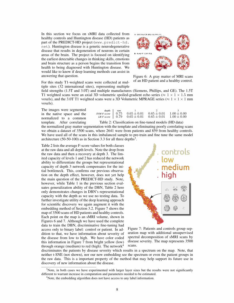
Figure 6: A gray matter of MRI scansof an HD patient and a healthy control.

In this section we focus on sMRI data collected fromhealthy controls and Huntington disease (HD) patients aspart of the PREDICT-HD project (www.predict-hd.net). Huntington disease is a genetic neurodegenerativedisease that results in degeneration of neurons in certainareas of the brain. The project is focused on identifyingthe earliest detectable changes in thinking skills, emotionsand brain structure as a person begins the transition fromhealth to being diagnosed with Huntington disease. Wewould like to know if deep learning methods can assist inanswering that question.

For this study T1-weighted scans were collected at mul-tiple sites (32 international sites), representing multiplefield strengths (1.5T and 3.0T) and multiple manufactures (Siemens, Phillips, and GE). The 1.5TT1 weighted scans were an axial 3D volumetric spoiled-gradient echo series (≈ 1 × 1 × 1.5 mmvoxels), and the 3.0T T1 weighted scans were a 3D Volumetric MPRAGE series (≈ 1 × 1 × 1 mmvoxels).

depth raw 1 2 3SVM F-score 0.75 0.65± 0.01 0.65± 0.01 1.00± 0.00

LR F-score 0.79 0.65± 0.01 0.65± 0.01 1.00± 0.00

Table 2: Classification on fine-tuned models (HD data)

The images were segmentedin the native space and thenormalized to a commontemplate. After correlatingthe normalized gray matter segmentation with the template and eliminating poorly correlating scanswe obtain a dataset of 3500 scans, where 2641 were from patients and 859 from healthy controls.We have used all of the scans in this imbalanced sample to pre-train and fine tune the same modelarchitecture (50-50-100) as in Section 3.3 for all three depths3.

Figure 7: Patients and controls group sep-aration map with additional unsupervisedspectral decomposition of sMRI scans bydisease severity. The map represents 3500scans.

Table 2 lists the average F-score values for both classesat the raw data and all depth levels. Note the drop fromthe raw data and then a recovery at depth 3. The lim-ited capacity of levels 1 and 2 has reduced the networkability to differentiate the groups but representationalcapacity of depth 3 network compensates for the ini-tial bottleneck. This, confirms our previous observa-tion on the depth effect, however, does not yet helpthe main question of the PREDICT-HD study. Note,however, while Table 1 in the previous section eval-uates generalization ability of the DBN, Table 2 hereonly demonstrates changes in DBN’s representationalcapacity with the depth as we use no testing data. Tofurther investigate utility of the deep learning approachfor scientific discovery we again augment it with theembedding method of Section 3.2. Figure 7 shows themap of 3500 scans of HD patients and healthy controls.Each point on the map is an sMRI volume, shown inFigures 6 and 7. Although we have used the completedata to train the DBN, discriminative fine-tuning hadaccess only to binary label: control or patient. In ad-dition to that, we have information about severity ofthe disease from low to high. We have color codedthis information in Figure 7 from bright yellow (low)through orange (medium) to red (high). The network4

discriminates the patients by disease severity which results in a spectrum on the map. Note, thatneither t-SNE (not shown), nor our new embedding see the spectrum or even the patient groups inthe raw data. This is a important property of the method that may help support its future use indiscovery of new information about the disease.

3Note, in both cases we have experimented with larger layer sizes but the results were not significantlydifferent to warrant increase in computation and parameters needed to be estimated.

4Note, the embedding algorithm does not have access to any label information.

8

4 ConclusionsOur investigations show that deep learning has a high potential in neuroimaging applications. Eventhe shallow RBM is already competitive with the model routinely used in the field: it producesphysiologically meaningful features which are (desirably) highly focal and have time course crosscorrelations that connect them into meaningful functional groups (Section 5). The depth of theDBN does indeed help classification and increases group separation. This is apparent on two sMRIdatasets collected under varying conditions, at multiple sites each, from different disease groups,and pre-processed differently. This is a strong evidence of DBNs robustness. Furthermore, ourstudy shows a high potential of DBNs for exploratory analysis. As Figure 7 demonstrates, DBNin conjunction with our new mapping method can reveal hidden relations in data. We did find itdifficult initially to find workable parameter regions, but we hope that other researchers won’t havethis difficulty starting from the baseline that we provide in this paper.

References[1] A. J. Bell and T. J. Sejnowski. An information-maximization approach to blind separation and

blind deconvolution. Neural Computation, 7(6):1129–1159, November 1995.[2] Bharat Biswal, F Zerrin Yetkin, Victor M Haughton, and James S Hyde. Functional connec-

tivity in the motor cortex of resting human brain using echo-planar mri. Magnetic resonancein medicine, 34(4):537–541, 1995.

[3] M.J. Brookes, M. Woolrich, H. Luckhoo, D. Price, J.R. Hale, M.C. Stephenson, G.R. Barnes,S.M. Smith, and P.G. Morris. Investigating the electrophysiological basis of resting state net-works using magnetoencephalography. Proceedings of the National Academy of Sciences,108(40):16783–16788, 2011.

[4] V. D. Calhoun, K. A. Kiehl, and G. D. Pearlson. Modulation of temporally coherent brainnetworks estimated using ICA at rest and during cognitive tasks. Human Brain Mapping,29(7):828–838, 2008.

[5] R. W. Cox et al. AFNI: software for analysis and visualization of functional magnetic reso-nance neuroimages. Computers and Biomedical Research, 29(3):162–173, 1996.

[6] T. de Vries, S. Chawla, and M. E. Houle. Finding local anomalies in very high dimensionalspace. In Proceedings of the 10th {IEEE} international conference on data mining, pages128–137. IEEE, IEEE Computer Society, 2010.

[7] Nate Derbinsky, Jose Bento, Veit Elser, and Jonathan S Yedidia. An improved three-weightmessage-passing algorithm. arXiv preprint arXiv:1305.1961, 2013.

[8] V. Elser, I. Rankenburg, and P. Thibault. Searching with iterated maps. Proceedings of theNational Academy of Sciences, 104(2):418, 2007.

[9] Nathan Swanson et. al. Lateral differences in the default mode network in healthy controls andpatients with schizophrenia. Human Brain Mapping, 32:654–664, 2011.

[10] Asja Fischer and Christian Igel. An introduction to restricted boltzmann machines. In Progressin Pattern Recognition, Image Analysis, Computer Vision, and Applications, pages 14–36.Springer, 2012.

[11] L. Freire, A. Roche, and J. F. Mangin. What is the best similarity measure for motion correctionin fMRI. IEEE Transactions in Medical Imaging, 21:470–484, 2002.

[12] Karl J Friston, Andrew P Holmes, Keith J Worsley, J-P Poline, Chris D Frith, and Richard SJFrackowiak. Statistical parametric maps in functional imaging: a general linear approach.Human brain mapping, 2(4):189–210, 1994.

[13] S. Gravel and V. Elser. Divide and concur: A general approach to constraint satisfaction.Physical Review E, 78(3):36706, 2008.

[14] Trevor. Hastie, Robert. Tibshirani, and JH (Jerome H.) Friedman. The elements of statisticallearning. Springer, 2009.

[15] G. Hinton and R. Salakhutdinov. Reducing the dimensionality of data with neural networks.Science, 313(5786):504–507, 2006.

[16] G. E. Hinton, S. Osindero, and Y. W. Teh. A fast learning algorithm for deep belief nets. Neuralcomputation, 18(7):1527–1554, 2006.

9

[17] Geoffrey Hinton. Training products of experts by minimizing contrastive divergence. NeuralComputation, 14:2002, 2000.

[18] P. O. Hoyer. Non-negative sparse coding. In Neural Networks for Signal Processing, 2002.Proceedings of the 2002 12th IEEE Workshop on, pages 557–565, 2002.

[19] Alex Krizhevsky, Ilya Sutskever, and Geoffrey E. Hinton. Imagenet classification with deepconvolutional neural networks. In Neural Information Processing Systems, 2012.

[20] Quoc V Le, Alexandre Karpenko, Jiquan Ngiam, and Andrew Y Ng. Ica with reconstructioncost for efficient overcomplete feature learning. In NIPS, pages 1017–1025, 2011.

[21] Quoc V. Le, Rajat Monga, Matthieu Devin, Kai Chen, Greg S. Corrado, Jeff Dean, and An-drew Y. Ng. Building high-level features using large scale unsupervised learning. In Interna-tional Conference on Machine Learning. 103, 2012.

[22] N. Le Roux and Y. Bengio. Deep belief networks are compact universal approximators. Neuralcomputation, 22(8):2192–2207, 2010.

[23] Jingyu Liu and Vince Calhoun. Parallel independent component analysis for multimodal anal-ysis: Application to fmri and eeg data. In Biomedical Imaging: From Nano to Macro, 2007.ISBI 2007. 4th IEEE International Symposium on, pages 1028–1031. IEEE, 2007.

[24] M. J. McKeown, S. Makeig, G. G. Brown, T. P. Jung, S. S. Kindermann, A. J. Bell, and T. J.Sejnowski. Analysis of fMRI data by blind separation into independent spatial components.Human Brain Mapping, 6(3):160–188, 1998.

[25] Shashwath A Meda, Nicole R Giuliani, Vince D Calhoun, Kanchana Jagannathan, David JSchretlen, Anne Pulver, Nicola Cascella, Matcheri Keshavan, Wendy Kates, Robert Buchanan,et al. A large scale (n= 400) investigation of gray matter differences in schizophrenia usingoptimized voxel-based morphometry. Schizophrenia research, 101(1):95–105, 2008.

[26] M. Moosmann, T. Eichele, H. Nordby, K. Hugdahl, and V. D. Calhoun. Joint independent com-ponent analysis for simultaneous EEG-fMRI: principle and simulation. International Journalof Psychophysiology, 67(3):212–221, 2008.

[27] Vinod Nair and Geoffrey E Hinton. Rectified linear units improve restricted boltzmann ma-chines. In Proceedings of the 27th International Conference on Machine Learning (ICML-10),pages 807–814, 2010.

[28] V. K. Potluru and V. D. Calhoun. Group learning using contrast NMF : Application to func-tional and structural MRI of schizophrenia. Circuits and Systems, 2008. ISCAS 2008. IEEEInternational Symposium on, pages 1336–1339, May 2008.

[29] Marcus E. Raichle, Ann Mary MacLeod, Abraham Z. Snyder, William J. Powers, Debra A.Gusnard, and Gordon L. Shulman. A default mode of brain function. Proceedings of theNational Academy of Sciences, 98(2):676–682, 2001.

[30] Sam T Roweis and Lawrence K Saul. Nonlinear dimensionality reduction by locally linearembedding. Science, (5500):2323–2326, 2000.

[31] Mikail Rubinov and Olaf Sporns. Weight-conserving characterization of complex functionalbrain networks. Neuroimage, 56(4):2068–2079, 2011.

[32] John W Sammon Jr. A nonlinear mapping for data structure analysis. Computers, IEEETransactions on, 100(5):401–409, 1969.

[33] Jing Sui, Tulay Adali, Qingbao Yu, Jiayu Chen, and Vince D. Calhoun. A review of multivari-ate methods for multimodal fusion of brain imaging data. Journal of Neuroscience Methods,204(1):68–81, 2012.

[34] Joshua B Tenenbaum, Vin De Silva, and John C Langford. A global geometric framework fornonlinear dimensionality reduction. Science, 290(5500):2319–2323, 2000.

[35] M.P. van den Heuvel and H.E. Hulshoff Pol. Exploring the brain network: A review on resting-state fMRI functional connectivity. European Neuropsychopharmacology, 2010.

[36] Laurens Van der Maaten and Geoffrey Hinton. Visualizing data using t-sne. Journal of MachineLearning Research, 9(2579-2605):85, 2008.

[37] Hui Zou, Trevor Hastie, and Robert Tibshirani. Sparse principal component analysis. Journalof computational and graphical statistics, 15(2):265–286, 2006.

10

5 Supplementary material

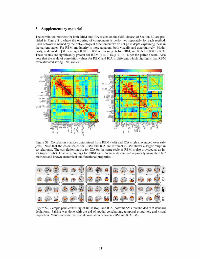
The correlation matrices for both RBM and ICA results on the fMRI dataset of Section 2.3 are pro-vided in Figure S1, where the ordering of components is performed separately for each method.Each network is named by their physiological function but we do not go in depth explaining these inthe current paper. For RBM, modularity is more apparent, both visually and quantitatively. Modu-larity, as defined in [31], averages 0.40± 0.060 across subjects for RBM, and 0.35± 0.056 for ICA.These values are significantly greater for RBM (t = 7.15, p < 1e−6 per the paired t-test). Alsonote that the scale of correlation values for RBM and ICA is different, which highlights that RBMoverestimated strong FNC values.

Figure S1: Correlation matrices determined from RBM (left) and ICA (right), averaged over sub-jects. Note that the color scales for RBM and ICA are different (RBM shows a larger range incorrelations). The correlation matrix for ICA on the same scale as RBM is also provided as an in-set (upper right). Feature groupings for RBM and ICA were determined separately using the FNCmatrices and known anatomical and functional properties.

Figure S2: Sample pairs consisting of RBM (top) and ICA (bottom) SMs thresholded at 2 standarddeviations. Pairing was done with the aid of spatial correlations, temporal properties, and visualinspection. Values indicate the spatial correlation between RBM and ICA SMs.

11